Multigrid convergence of discrete geometric estimators this chapter, we use DGtal to represent...

Multigrid convergence of discrete geometricestimators

D. Coeurjolly1, J.-O. Lachaud2, and T. Roussillon1

Abstract The analysis of digital shapes require tools to determine accurately theirgeometric characteristics. Their boundary is by essence discrete and is seen by con-tinuous geometry as a jagged continuous curve, either straight or not derivable.Dis-crete geometric estimatorsare specific tools designed to determine geometric infor-mation on such curves. We present here global geometric estimators of area, length,moments, as well as local geometric estimators of tangent and curvature. We furtherstudy theirmultigrid convergence, a fundamental property which guarantees thatthe estimation tends toward the exact one as the sampling resolution gets finer andfiner. Known theorems on multigrid convergence are summarized. A representativesubsets of estimators have been implemented in a common framework (the libraryDGtal), and have been experimentally evaluated for several classes of shapes. Theinterested user has thus all the information for choosing the estimator best adaptedto its application, and disposes readily of an efficient implementation.

1 Introduction

Since early developments in image processing and image understanding, many toolshave been developed in order to quantify the geometry of a digital shape. Suchdigital shapes can be defined for instance either from a segmentation process assubset of image pixels sharing the same colorimetric information, or as the result ofthe digitization of a continuous object.

In many applications, it is important to have a geometrical quantification or de-scription from measurements which are invariant under a specific class of transforms(rotation, translation, scaling, . . . ) or which preserve important geometrical features

1 University of Lyon / CNRS, LIRIS, UMR CNRS 5205, F-69676, FRANCEe-mail:david.coeurjolly|[email protected] University of Savoie, LAMA, UMR CNRS 5127, F-73376 Le Bourget du Lace-mail:[email protected]

1

2 D. Coeurjolly, J.-O. Lachaud, and T. Roussillon

(characteristic points, local convexity, . . . ). In this context, we usually consider dif-ferential or integral quantities evaluated either on the digital shape or its boundary.Beside such type of quantification, we can distinguish two classes of geometrical de-scriptors. The first class corresponds to global descriptors which associate a globalnumerical quantity to each shape. In this class, we have arc length or perimeter esti-mators of digital shape boundaries, but also integral quantities such as geometricalmoments approximated on the digital shape. The second classcontains local esti-mators which usually associate a numerical quantity to eachpoint of the shape. Forexample, curvature or normal vector estimators at boundarypoints belong to thisclass.

When defining an algorithm that evaluate such descriptors ondigital shape, socalled estimator, the evaluation of such estimator accuracy may be challenging. Inthe literature, several approaches have been proposed. Thefirst one is applicationdriven and consists in validating the estimators within a complete shape descriptionpipeline. For instance, one can evaluate a curvature estimator in a global character-istic points estimation framework of contours.

One can also evaluate the accuracy of the estimator in terms of expected prop-erties. For instance, we can evaluate the stability of a curvature estimator whenrotations of input shapes are given.

A more formal evaluation process consists in comparing the estimated quanti-ties with exact Euclidean values on a family of continuous shapes in a multigridasypmptotic framework. More precisely, letX be a family of compact simply con-nected subsets ofR2 with continuous curvature fields. We denote byD(X,h) theGauss digitization ofX ∈ X with grid steph, seen as a union of pixels of sidehin R2. For sake of clarity, we shorten in the sequelD(X,h) into D and denote itscomplementary byD. Moreover, let us assume thatD contains at least one pixel, i.e.|D| ≥ 1.

In this multigrid framework, comparing the estimated quantity to the expectedEuclidean one whenh tends to zero is called themultigrid convergenceanalysis ofan estimator [32]. Indeed, at a given resolution, infinitelymany shapes have the samedigitization, which hampers the objective comparison of estimators. For estimatorsof local geometric quantities like tangent or curvature, few results exist. We mayquote some convergence results for tangent estimators [39,48, 19]. And there is nocorrect convergence results for curvature as far as we know.

In this chapter, we use this multigrid comparison frameworkin order to reviewand evaluate existing local and global estimators on digital shapes. A important con-tribution is to have considered a large set of estimators in aunique technical frame-work: the DGtal opensource library [1]. DGtal is a generic open source library forDigital Geometry programming for which the main objective is to structure differentdevelopments from the digital geometry and topology community. For the purposeof this chapter, we use DGtal to represent multigrid digitalobjects and shapes, todefine the geometric estimators and we provide ways to compare estimated valuesto expected Euclidean ones.

The chapter is organised as follows: Sect. 2 focuses on global estimators (area,moments and arc length) and Sect. 3 is devoted to local estimators (tangent, cur-

Multigrid convergence of discrete geometric estimators 3

vature). In both cases, each section starts with formal definition of the multigridconvergence of an estimator. In Sect. 6, we discuss on implementation details ofboth the estimator and the comparative evaluation framework.

2 Global Estimators

2.1 Multigrid convergence for global estimators

Multigrid convergence is an interesting way of relating digital and Euclidean ge-ometries. The idea is to ask for discrete geometric estimations to converge towardthe corresponding Euclidean quantity when considering finer and finer shape digi-tizations (here, Gauss digitization). The following definition is taken from Defini-tion 2.10 of [32].

Definition 1 (Multigrid convergence for global geometric quantities).A discretegeometric estimatorE of some geometric quantityE is multigrid convergentfor afamily of shapesX and a digitization processD iff for all shapeX ∈ X, there existsa grid stephX > 0 such that the estimateE(D(X,h),h) is defined for all 0< h< hX

and|E(D(X,h),h)−E(X)| ≤ τX(h),

whereτX : R+ →R+ with null limit at 0. This function is thespeed of convergenceof the estimator.

The convergence of most estimators depends on the family of shapes in the Eu-clidean plane that is considered. We therefore introduce several standard familiesthat will be used to define the range of validity of multigrid convergence theorems.A curve is said to beCn if it has continuousn-th order derivatives.

• The family of all finite convex shapes in the Euclidean plane is denoted withXC.• The family of convex sets whose boundary is aCn arc with positive curvature

everywhere is denoted byXn−SC.• The family of all planar piecewisen-smooth convex set is denoted with

Xn−PW−SC. These sets are convex sets whose boundary consists of a finite num-ber ofCn arcs with positive curvature everywhere except at arc endpoints. ClearlyXn−SC(Xn−PW−SC.

For experiments, we will use shapes that are representativeof these families.Several representative shapes digitized at different scales are illustrated on Fig. 1.They will be used for the upcoming experiments on global and local geometricestimators.


Square Triangle Circle

(a) 1 (b) 0.1 (c) 1 (d) 0.1 (e) 1 (f) 0.1Ellipse Flower Accflower

(g) 1 (h) 0.1 (i) 1 (j) 0.1 (k) 1 (l) 0.1

Fig. 1 Digitization at two different grid steps (h = 1 or h = 0.1) of tests shapes: (a-d) the squareand triangle are inXC; the circle (e,f) and the ellipse (g,h) belongs toX3-SC; the flower (i,j), andthe “accflower” (k,l) are inX3-PW-SC. All shapes have a diameter 20.

2.2 Area and moments

Designing a multigrid convergent estimator of the area is fairly simple. We definethearea estimator by countingA as

A(Y,h) = h2 ∑(i, j)∈Y

1, (1)

whereY is an arbitrary digital shape andh the gridstep. This estimator just countsthe number ofh-grid square inY and normalizes the result with the area of each gridsquare.

As reported in [33], Gauss and Dirichlet knew already that this area estimatorwas multigrid convergent for finite convex shape (XC) with a speedO(l ·h), where

l is the shape perimeter. Huxley [26] improves the bound toO(h1511(log 1

h)4722) for

the familyX3−PW−SC. This simple estimator has thus superlinear convergence for arather wide class of shapes.

Klette andZunic [33] follows the idea of (1) to design thediscrete(p,q)-momentestimatormp,q, for integersp,q≥ 0, as follows:

mp,q(Y,h) = h2+p+q ∑(i, j)∈Y

ip · jq. (2)

These estimators approximate the(p,q)-moments of a shapeX, which are de-fined asmp,q(X) =

∫∫X xpyqdxdy. Their speed of convergence is sumed up in Tab. 1.

In a similar way, central moments may be approximated. We refer the reader to [33]for further details. Note that moments can be used to determine for instance thecenter of gravity or the orientation of a shape. Furthermore, several rotational in-variant quantities can be obtained as combination of(p,q)-moments. For instance,


Zernike and Legendre moments widely used in many 2D and 3D shape indexing andretrieval are linear combination of(p,q)-moments [64, 53]. Hence, convergence re-sults on(p,q)-moments lead to convergecne of Zernike and Legendre moments aswell.

The previous estimators require to visit all points of the digital object, andnot only its boundary. The computational complexity of these estimators is thusO(1/h2). However, a discrete variant of Green theorem allows to compute thesequantities by simply visiting the shape boundary, thus reducing the computationalcomplexity toO(1/h) for convex shapes. See Lien [44] for a generic discrete Greentheorem framework and Brleket al. for a digital geometry application [5].

2.3 Perimeter and length estimators

It is more complex to estimate the perimeter of a digital shape. Indeed, enumeratingthe number of grid steps of the digital shape boundary does not lead to a reliableperimeter estimator. It is called thenaive perimeter estimatorLnaive and is definedas

Lnaive(Y,h) = h ∑σ∈∂Y

1. (3)

This estimator overestimates the shape perimeter. Indeed,it is clear that it alwaysreturns the perimeter of the axis-aligned bounding box of the shape.

Therefore first approaches to length estimation tried to assign different weightsto different local configurations so as to be more precise. The Rosen-Proffitt esti-mator [56] and BLUE (best linear unbiased) estimator [17] belong to this category.However it was proven in Tajine and Daurat [63] that all theseapproaches can neverachieve multigrid convergence, whatever the (finite) number of configurations takeninto account.

More complex approaches are required to achieve convergence. We list belowseveral of them, which are also experimentally compared (see Fig. 2). Most of themare not only valid for perimeter estimation but also for curve length estimation.

• The DSS length estimatorLDSS, proposed by Kovalevsky and Fuchs [34], re-lies on a greedy decomposition of the input digital contour into Digital StraightSegments (DSS). It starts from a point, then find the longest DSS starting fromthis point. The end point of this DSS defines a new starting point. The processis repeated till the whole contour has been visited. The DSS end points forma polygonal line. The length or perimeter of the digital contour is then simplydefined as Euclidean length of this polygonal line.

• The MLP length estimatorLMLP, proposed by Slobodaet al. [62], also relieson a polygonal approximation of the digital contour. For a given simple digitalshape, the Minimum Length Polygon (MLP) is indeed the shortest Euclideancurve which separates the interior pixel centers from the exterior pixel centers.


The length is then defined as the perimeter of this curve. Several linear-timealgorithms for computing the MLP are available [57, 61].

• TheFP length estimatorLFP, proposed in [61], relies on yet another polygonalapproximation of the digital contour. One can see it is a translated version of theMLP, where convex turns are translated outwards and concaveturns are trans-lated inwards by half-unit diagonal vectors. The advantageis that the polygonvertices form a subset of the grid points of the input contour.

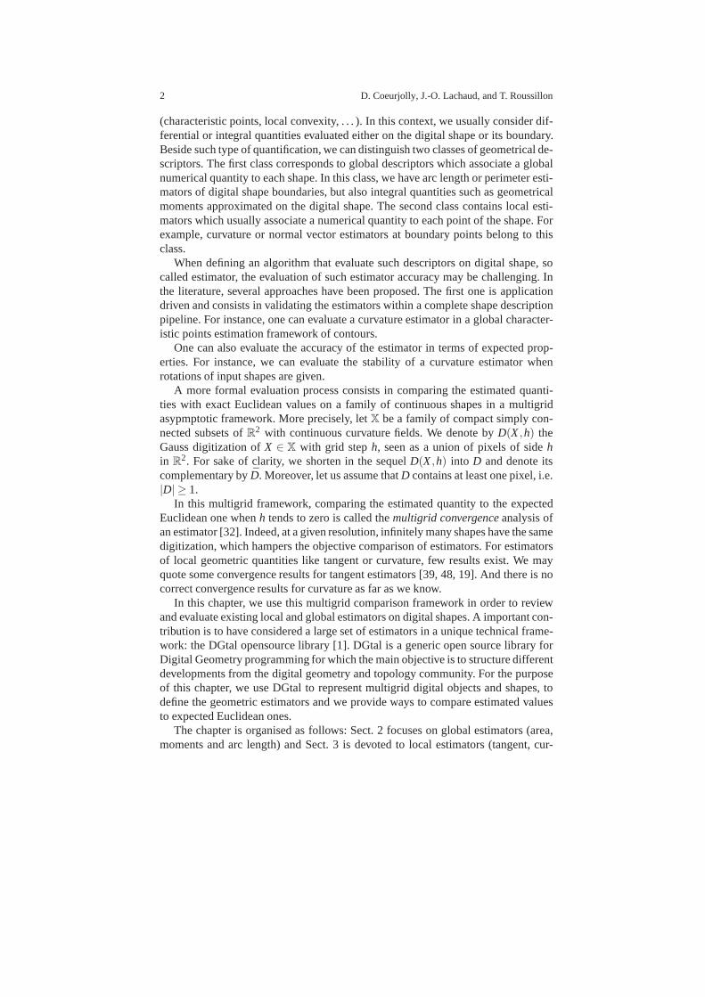
• Another approach to local length estimation and thus perimeter estimation is tointegrate the tangent estimation along the curve [10, 13] (see next section ontangent estimation too). TheST length estimatorLST is based on the symmet-ric tangent while theλ -MST length estimatorLλ -MST is based on theλ -convexcombination of maximal segments [39]. More precisely, if a grid edgeσ has di-rection vectort(σ) and estimated unit tangent vectorT(σ), these two estimatorsare defined as:

LST(Y,h) = h ∑σ∈∂Y

TST(σ) · t(σ), Lλ -MST(Y,h) = h ∑σ∈∂Y

Tλ -MST(σ) · t(σ).

(4)

1e-06

1e-05

0.0001

0.001

0.01

0.1

1

0.001 0.01 0.1 1

NaiveBLUE

RosenProffittDSSMLP

FPST

l-MST 1e-06

1e-05

0.0001

0.001

0.01

0.1

1

0.001 0.01 0.1 1

NaiveBLUE

RosenProffittDSSMLP

FPST

l-MST

Ball of radius 10 Square of side 10√

2 and rotated of 0.5 rad.

Fig. 2 Absolute relative error for several length and perimeter estimators. It is a clear that the naivelength estimator does not converge. The other estimators (DSS, MLP, FP, ST,λ -MST) present amultigrid convergence. Note that experimentally the convergence speed for DSS, FP, and ST on the

ball is O(h) while MLP andλ -MST achieve a better bound ofO(h43 ). However, on the boundary

of a shape with linear parts, the convergence speed isO(h) for all the estimators except the naiveone.

Some experimental evaluation of the multigrid convergencehas been carried outfor these estimators and is illustrated on Fig. 2. It appearsthat the perimeter ofshapes with rectilinear boundaries is accurately estimated with any of the presentedlength estimators but for the naive one. However, for shapeswith sufficiently smoothboundaries and positive curvature, the MLP andλ -MST have superlinear conver-gence and should be preferred. Note finally that only DSS, MLP, andλ -MST haveproven multigrid convergence, but the found bounds are not necessarily tight. In


0

200

400

600

800

1000

1200

1400

1600

1800

2000

0 1e+06 2e+06 3e+06 4e+06 5e+06 6e+06 7e+06 8e+06

NaiveBLUE

RosenProffittDSSMLP

FP

0

500

1000

1500

2000

2500

3000

0 1e+06 2e+06 3e+06 4e+06 5e+06 6e+06 7e+06 8e+06 9e+06 1e+07

NaiveBLUE

RosenProffittDSSMLP

FP

Ball of radius 1000 Square of side 1000√

2 and rotated of 0.5 rad.

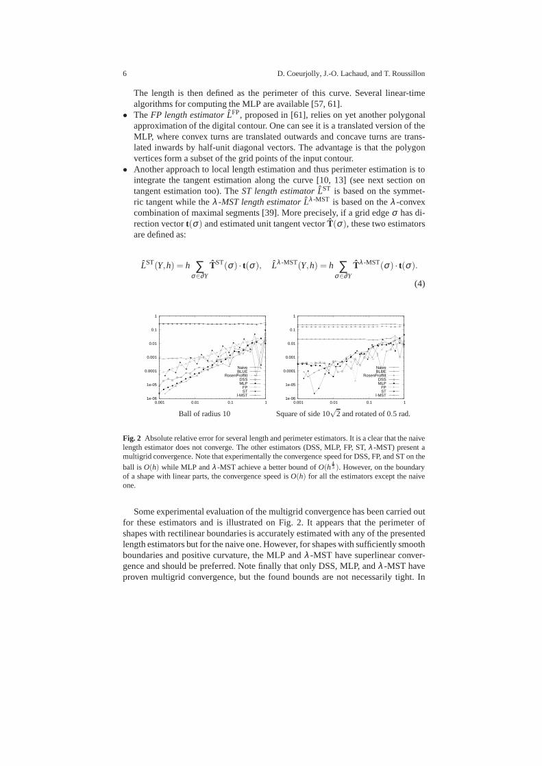
Fig. 3 Computation time for length estimators implemented in DGtal (Naive, BLUE, RosenProf-fitt, DSS, MLP, FP). For the sake of clarity, abscissa corresponds to the size of the contour innumber of grid points. Ordinate corresponds to timings in millisecond (Intel Xeon 2.27GHz, DG-tal 0.4).

Fig. 3, we present computational time for estimators implemented in DGtal release0.4 (Naive, BLUE, RosenProffitt, DSS, MLP, FP). Convergenceresults for ST andλ -MST have been obtained from ImaGene library [2]. In these graphs, we can ob-serve the linear computational cost of all estimators with respect to the size of thecontours. As expected, local estimators outperform the other ones but DSS basedestimator is a good compromise between efficiency and theoretical multigrid con-vergence.

2.4 Summary

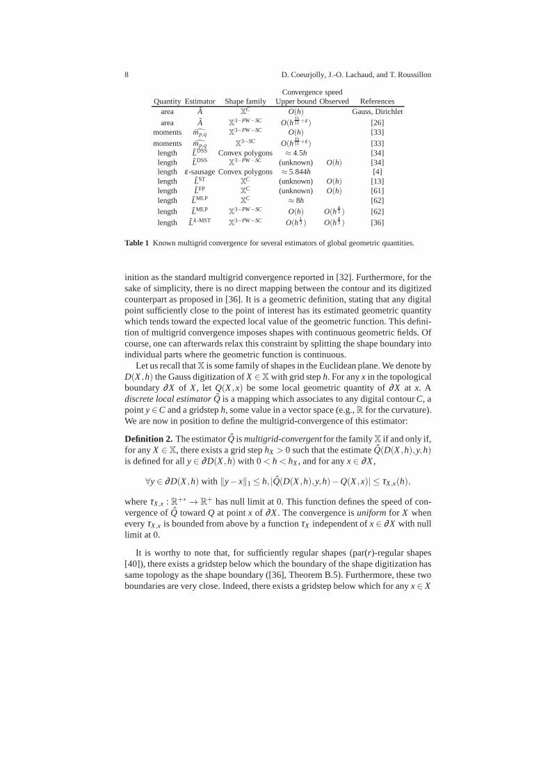
Tab. 1 summarizes multigrid convergence results for estimators of global geometricquantities. It appears that some theoretical bounds are nottight and that some othersare yet to be proven.

3 Local Estimators

3.1 Multigrid convergence for local estimators

Tangent direction, normal vector, curvature are local geometric quantities along theshape boundary. Each of them is thus some function of the shape boundary. How-ever, the contour of the shape digitization does not define the same domain. There-fore we cannot directly compare the true geometric functionwith the estimated geo-metric function. We provide below a definition of multigrid convergence for discretelocal estimators. It is neither a parametric definition as in[19] nor a point-wise def-


Convergence speedQuantity Estimator Shape family Upper bound Observed References

area A XC O(h) Gauss, Dirichlet

area A X3−PW−SC O(h1511+ε) [26]

moments mp,q X3−PW−SC O(h) [33]

moments mp,q X3−SC O(h1511+ε) [33]

length LDSS Convex polygons ≈ 4.5h [34]length LDSS X3−PW−SC (unknown) O(h) [34]length ε-sausage Convex polygons≈ 5.844h [4]length LST XC (unknown) O(h) [13]length LFP XC (unknown) O(h) [61]length LMLP XC ≈ 8h [62]

length LMLP X3−PW−SC O(h) O(h43 ) [62]

length Lλ -MST X3−PW−SC O(h13 ) O(h

43 ) [36]

Table 1 Known multigrid convergence for several estimators of global geometric quantities.

inition as the standard multigrid convergence reported in [32]. Furthermore, for thesake of simplicity, there is no direct mapping between the contour and its digitizedcounterpart as proposed in [36]. It is a geometric definition, stating that any digitalpoint sufficiently close to the point of interest has its estimated geometric quantitywhich tends toward the expected local value of the geometricfunction. This defini-tion of multigrid convergence imposes shapes with continuous geometric fields. Ofcourse, one can afterwards relax this constraint by splitting the shape boundary intoindividual parts where the geometric function is continuous.

Let us recall thatX is some family of shapes in the Euclidean plane. We denote byD(X,h) the Gauss digitization ofX ∈X with grid steph. For anyx in the topologicalboundary∂X of X, let Q(X,x) be some local geometric quantity of∂X at x. Adiscrete local estimatorQ is a mapping which associates to any digital contourC, apointy∈C and a gridsteph, some value in a vector space (e.g.,R for the curvature).We are now in position to define the multigrid-convergence ofthis estimator:

Definition 2. The estimatorQ ismultigrid-convergentfor the familyX if and only if,for anyX ∈X, there exists a grid stephX > 0 such that the estimateQ(D(X,h),y,h)is defined for ally∈ ∂D(X,h) with 0< h< hX, and for anyx∈ ∂X,

∀y∈ ∂D(X,h) with ‖y− x‖1 ≤ h, |Q(D(X,h),y,h)−Q(X,x)| ≤ τX,x(h),

whereτX,x : R+∗ → R+ has null limit at 0. This function defines the speed of con-vergence ofQ towardQ at pointx of ∂X. The convergence isuniform for X wheneveryτX,x is bounded from above by a functionτX independent ofx∈ ∂X with nulllimit at 0.

It is worthy to note that, for sufficiently regular shapes (par(r)-regular shapes[40]), there exists a gridstep below which the boundary of the shape digitization hassame topology as the shape boundary ([36], Theorem B.5). Furthermore, these twoboundaries are very close. Indeed, there exists a gridstep below which for anyx∈ X


there is ay∈ ∂D(X,h) with ‖y−x‖1 ≤ h and conversely for anyy∈ ∂D(X,h), thereis ax∈ X with ‖y− x‖1 ≤ h ([36], Lemma B.9).

Therefore the previous definition of multigrid convergenceguarantees that theestimated local quantity converges toward the true local geometric quantity every-where along the shape boundary.

3.2 Methodology for experimental evaluation

When multigrid convergence theorems have been established, we will referencethem and indicate the known convergence rate. We nevertheless carry out an experi-mental evaluation of many different estimators for two reasons: (1) few convergencetheorems exist for local estimators, (2) practical error bounds at finite scale are alsoimportant for the end-user.

In the next sections, we apply the following methodology foranalyzing estima-tors:

1. Test shapes. We use the shapes of Fig. 1 for the experiments. They are repre-sentative of the different shape families that we are studying. Indeed, shapescomposed of linear parts, smooth parts and corners, arise naturally in imageanalysis. When the tangent field is not continuous (square, triangle), only theaverage error is significant.

2. Graphs of estimations with respect to ground truth. We display the graphs of theestimated values for different estimators (functionsQ) and the expected graph(functionQ).

3. Error measures for decreasingh. We study the following measures:

εabs(X,y,h) = |Q(X,x(y))− Q(D(X,h),y,h)| (5)

or (when vectorial) εabs(X,y,h) = |det(Q(X,x(y)),Q(D(X,h),y,h)| (6)

εrel(X,y,h) =εabs(X,y,h)|Q(X,x(y))| (7)

εabs(X,h) =1

#D(X,h) ∑y∈D(X,h)

εabs(X,y,h) (8)

ε rel(X,h) =1

#D(X,h) ∑y∈D(X,h)

εrel(X,y,h) (9)

(10)

Herex(·) is a mapping associating to each digitized point a point on the shapeboundary that is close enough (‖y−x(y)‖1 ≤ h). The same mapping is used forall estimators.

4. When known, computational complexities for computing estimators will begiven. Otherwise, for fair comparisons, we only measure computation timesfor estimators implemented in the DGtal library (see Section 6).


This methodology allows us to evaluate experimentally the accuracy and multi-grid convergence properties of discrete local geometric estimators. Section 4 studiestangent estimators and Section 5 studies curvature estimators. Their implementationin a common framework is discussed in Section 6.

4 Tangent

The aim of tangent estimators is to determine what is locallythe shape boundarydirection. For curvesγ(s) (at leastC1) defined as functions of a curvilinear abscissas, the tangent vector is defined asdγ

ds, which is a unit vector. The tangent directionφ(s) is defined as the angle between thex-axis and this unit vector.

4.1 Tangent estimators

Given a digital contour and a digital point, tangent estimators return a unit vector.For easier view, it is also possible to plot the angle of the tangent vector wrtx-axis.It is clear that the grid edge direction (see arrows in Fig. 9-(d) for an illustration)is a very bad tangent estimator, since on any shape inX1-SC it will have points withεabs or εrel close toπ

2 .More complex approaches are necessary. Digital tangent estimators have been

thoroughly compared in [38, 39]. They have been compared to continuous ap-proaches in [66, 67]. We describe below some representativetangent estimators,which will be compared experimentally.

• A first natural approach is to use a local least-square fit of a polynomial [7, 43].These techniques define a fixed window-sizeq. Around the point of interest theyuse 2q+ 1 samples which are used to find the polynomial of given degreethatbest fit these data in the least-square sense. We focus here onlow-degree polyno-mials. TheLR tangent estimatorTLR-q is the linear-regression with the windowsizeq. The ICIPF tangent estimatorTICIPF-q is the implicit parabola fitting ofwindow sizeq, made independently on each coordinate. They were found to berepresentative of that kind of methods [66, 67].

• A second approach is to see the digital contour as a discrete signal (x[t],y[t])and to convolve this signal with a Gaussian derivative of given kernelσ . Thisis very similar to the binomial convolution approach of [48,19, 21]. Therefore,we choose theH1-0GD tangent estimatorTH1-0GD [67], which defines locallythe window size as the longest maximal digital straight containing the point. A

slight variant is proven to be multigrid convergent inO(h13 ) for smooth shapes

in X3−SC, while its experimental convergent rate is excellent [67] for smoothshapes.


• TheMCMS tangent estimatorTMCMS defines the tangent as the direction of themost-centered maximal digital straight segment containing the point of interest[20]. It is proven to be uniformly multigrid convergent inO(h

13 ) in [36, 39].

• the λ -MST tangent estimatorTλ -MST is based on theλ -convex combination ofthe direction of the maximal digital straight segments containing the point ofinterest [39]. The functionλ is a mapping governing the way these directions arecombined. We use here a simple triangle functionf , such thatf (0) = 0, f (1) =

0, f (0.5) = 1. It is proven to be uniformly multigrid convergent inO(h13 ) in [36,

39].• the BC tangent estimatorTBC see the digital contour as a discrete signal

(x[t],y[t]) and convolves it with discrete binomials and a discrete difference op-erator, so as to mimick the convolution by a Gaussian derivative [48, 19]. We usethe suggested mask size ofd.h−

43 , whered is the continuous shape diameter. It

is proven to be uniformly multigrid convergent inO(h23 ) in [48].

• TheMATAS tangent estimatorTMATASis an adaptation of the median filter com-monly used in image processing [50]. If(Pi) are the vertices of the grid contour,this method consists in choosing the median orientation among the following 2qvectors centered onPi: (Pi−qPi, . . . ,Pi−1Pi ,PiPi+1, . . . ,PiPi+q).

4.2 Experimental evaluation

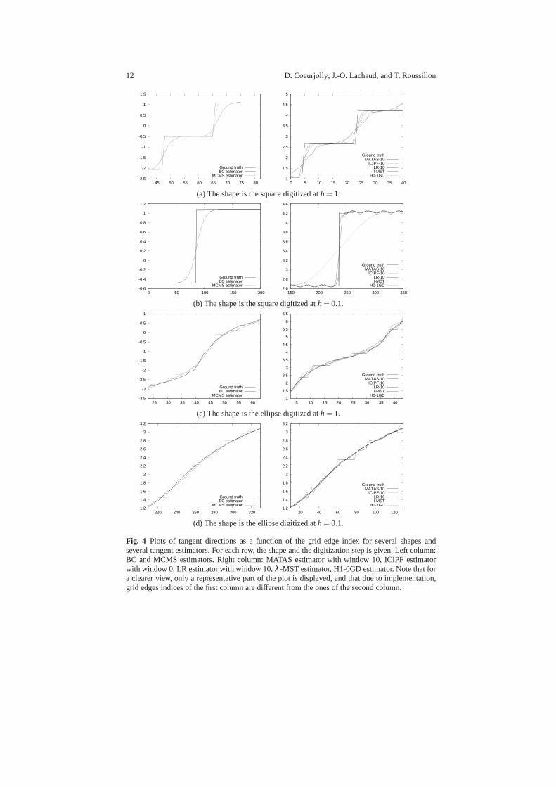
We have run these estimators on two representative shapes (the square is represen-tative ofXC, the ellipse is representative ofX3-SC) at different steps (coarseh= 1,mediumh = 0.1): results are displayed on Fig. 4. Only MCMS andλ -MST de-tect perfectly straight parts and corners. Others tend to smooth around corners, theamount of smoothing being dependent on the (chosen) size of the window. Fur-thermore, LR and ICIPF oscillate around the correct value onstraight parts. It ismore difficult to tell which estimator is the best along the boundary of smoothcurved parts. MCMS produces a staircase-like function but keeps the convexity ofthe shape. MATAS, LR and ICIPF may also oscillate and create false concavities.BC andλ -MST follow nicely the ground truth function. Overall,λ -MST seemsthe most versatile and accurate at these resolutions. Experiments on other shapesconfirm the presented behaviors of these estimators.

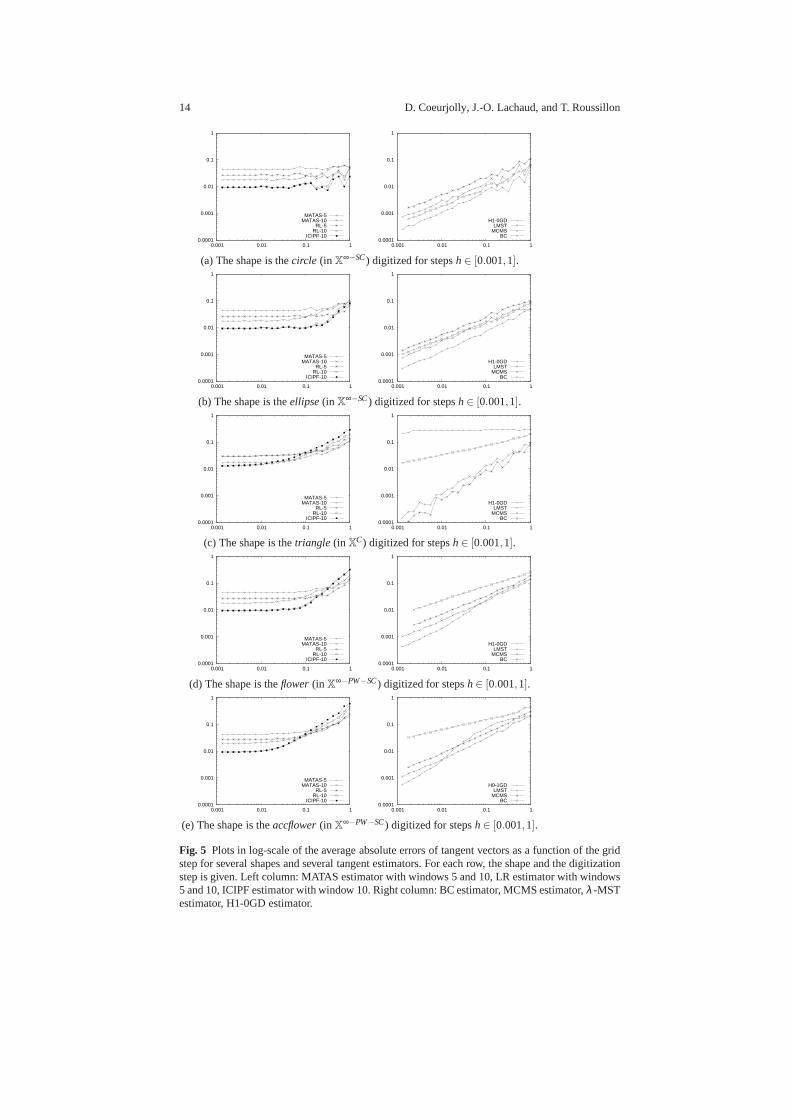
We now turn ourselves to the asymptotic behavior of these estimators, namelytheir possible multigrid convergence. We focus on the average absolute error of thetangent vector, i.e.εabs(X,h) (see (8)). The error plots displayed on Fig. 5 show thattangent estimators with fixed window size are not multigrid convergent. This is thecase of RL, ICIPF and MATAS estimators. Interestingly, but not surprisingly, smallwindow sizes bring better precision at low scale while greater window sizes bringbetter precision at fine scale. This is clearly the problem ofsuch estimators: theyrequire a user to choose the best possible scale according tothe input data.


-2.5

-2

-1.5

-1

-0.5

0

0.5

1

1.5

45 50 55 60 65 70 75 80

Ground truthBC estimator

MCMS estimator 1

1.5

2

2.5

3

3.5

4

4.5

5

0 5 10 15 20 25 30 35 40

Ground truthMATAS-10

ICIPF-10LR-10l-MST

H0-1GD

(a) The shape is the square digitized ath= 1.

-0.6

-0.4

-0.2

0

0.2

0.4

0.6

0.8

1

1.2

0 50 100 150 200


MCMS estimator 2.6

2.8

3

3.2

3.4

3.6

3.8

4

4.2

4.4

150 200 250 300 350


ICIPF-10LR-10l-MST

H0-1GD

(b) The shape is the square digitized ath= 0.1.

-3.5

-3

-2.5

-2

-1.5

-1

-0.5

0

0.5

1

25 30 35 40 45 50 55 60


MCMS estimator 1

1.5

2

2.5

3

3.5

4

4.5

5

5.5

6

6.5

5 10 15 20 25 30 35 40


ICIPF-10LR-10l-MST

H0-1GD

(c) The shape is the ellipse digitized ath= 1.

1.2

1.4

1.6

1.8

2

2.2

2.4

2.6

2.8

3

3.2

220 240 260 280 300 320


MCMS estimator 1.2

1.4

1.6

1.8

2

2.2

2.4

2.6

2.8

3

3.2

20 40 60 80 100 120


ICIPF-10LR-10l-MST

H0-1GD

(d) The shape is the ellipse digitized ath= 0.1.

Fig. 4 Plots of tangent directions as a function of the grid edge index for several shapes andseveral tangent estimators. For each row, the shape and the digitization step is given. Left column:BC and MCMS estimators. Right column: MATAS estimator with window 10, ICIPF estimatorwith window 0, LR estimator with window 10,λ -MST estimator, H1-0GD estimator. Note that fora clearer view, only a representative part of the plot is displayed, and that due to implementation,grid edges indices of the first column are different from the ones of the second column.


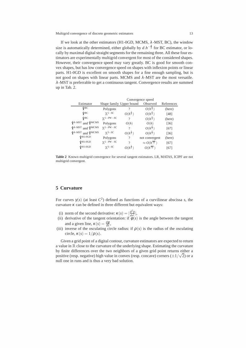
If we look at the other estimators (H1-0GD, MCMS,λ -MST, BC), the windowsize is automatically determined, either globally byd.h−

43 for BC estimator, or lo-

cally by maximal digital straight segments for the remaining three. All these four es-timators are experimentally multigrid convergent for mostof the considered shapes.However, their convergence speed may vary greatly. BC is good for smooth con-vex shapes, but has low convergence speed on shapes with inflexion points or linearparts. H1-0GD is excellent on smooth shapes for a fine enough sampling, but isnot good on shapes with linear parts. MCMS andλ -MST are the most versatile.λ -MST is preferrable to get a continuous tangent. Convergence results are summedup in Tab. 2.

Convergence speedEstimator Shape family Upper bound Observed References

TBC Polygons ? O(h13 ) (here)

TBC X1−SC O(h23 ) O(h

23 ) [48]

TBC X1−PW−SC ? O(h13 ) (here)

Tλ -MST andTMCMS Polygons O(h) O(h) [36]

Tλ -MST andTMCMS X1−PW−SC ? O(h23 ) [67]

Tλ -MST andTMCMS X3−SC O(h13 ) O(h

23 ) [36]

TH1-0GD Polygons ? not convergent (here)

TH1-0GD X1−PW−SC ? ≈ O(h2.53 ) [67]

TH1-0GD X3−SC O(h13 ) O(h

2.53 ) [67]

Table 2 Known multigrid convergence for several tangent estimators. LR, MATAS, ICIPF are notmultigrid convergent.

5 Curvature

For curvesγ(s) (at leastC2) defined as functions of a curvilinear abscissas, thecurvatureκ can be defined in three different but equivalent ways:

(i) norm of the second derivative:κ(s) = |d2γds2

|,(ii) derivative of the tangent orientation: ifφ(s) is the angle between the tangent

and a given line,κ(s) = dφds ,

(iii) inverse of the osculating circle radius: ifρ(s) is the radius of the osculatingcircle,κ(s) = 1/ρ(s).

Given a grid point of a digital contour, curvature estimators are expected to returna value inR close to the curvature of the underlying shape. Estimating the curvatureby finite differences over the two neighbors of a given grid point returns either apositive (resp. negative) high value in convex (resp. concave) corners (±1/

√2) or a

null one in runs and is thus a very bad solution.


0.0001

0.001

0.01

0.1

1

0.001 0.01 0.1 1

MATAS-5MATAS-10

RL-5RL-10

ICIPF-10 0.0001

0.001

0.01

0.1

1

0.001 0.01 0.1 1

H1-0GDLMST

MCMSBC

(a) The shape is thecircle (in X∞−SC) digitized for stepsh∈ [0.001,1].

0.0001

0.001

0.01

0.1

1

0.001 0.01 0.1 1

MATAS-5MATAS-10

RL-5RL-10

ICIPF-10 0.0001

0.001

0.01

0.1

1

0.001 0.01 0.1 1

H1-0GDLMST

MCMSBC

(b) The shape is theellipse(in X∞−SC) digitized for stepsh∈ [0.001,1].

0.0001

0.001

0.01

0.1

1

0.001 0.01 0.1 1

MATAS-5MATAS-10

RL-5RL-10

ICIPF-10 0.0001

0.001

0.01

0.1

1

0.001 0.01 0.1 1

H1-0GDLMST

MCMSBC

(c) The shape is thetriangle (in XC) digitized for stepsh∈ [0.001,1].

0.0001

0.001

0.01

0.1

1

0.001 0.01 0.1 1

MATAS-5MATAS-10

RL-5RL-10

ICIPF-10 0.0001

0.001

0.01

0.1

1

0.001 0.01 0.1 1

H1-0GDLMST

MCMSBC

(d) The shape is theflower (in X∞−PW−SC) digitized for stepsh∈ [0.001,1].

0.0001

0.001

0.01

0.1

1

0.001 0.01 0.1 1

MATAS-5MATAS-10

RL-5RL-10

ICIPF-10 0.0001

0.001

0.01

0.1

1

0.001 0.01 0.1 1

H0-1GDLMST

MCMSBC

(e) The shape is theaccflower(in X∞−PW−SC) digitized for stepsh∈ [0.001,1].

Fig. 5 Plots in log-scale of the average absolute errors of tangentvectors as a function of the gridstep for several shapes and several tangent estimators. Foreach row, the shape and the digitizationstep is given. Left column: MATAS estimator with windows 5 and 10, LR estimator with windows5 and 10, ICIPF estimator with window 10. Right column: BC estimator, MCMS estimator,λ -MSTestimator, H1-0GD estimator.


Many curvature estimators have been proposed in the literature to cope with thisproblem. They are roughly based on one of the three above-mentioned definitionsas it has been noticed in [70, 25].

In methods (i) and (ii), derivatives are often approximatedfrom the convolutionof either the tangent orientation [70, 65, 20] (i), or the digital contour viewed as adiscrete signal(x[t],y[t]) [48, 19, 21] (ii). They can also be computed from somepolynomials of a given degree locally fitted to the digital contour [49, 25].

Tangents and osculating circles used in methods (ii) and (iii) often relies on fit-ting techniques, either in a continuous setting (least square line or arc fitting [70]), orin a discrete setting to limit the arithmetic effects: digital straight segments [65, 20],digital level layers (extension to polynomials of higher degrees) [58, 23], approx-imation of the osculating circle with digital straight segments [14, 15, 25], digitalcircular arcs [60].

In most approaches, a user-given window or smoothing parameter is used so asto remove the jaggedness of digital contours and to make it continuous [70, 65, 20,46, 48, 19, 21, 22]. Few curvature estimators do not require an external parameterand we chose to focus on these methods.

5.1 Curvature estimators

The curvature estimators that do not require any parameter either rely on discreteprimitives such as digital straight segment (DSS), digitalcircular arc (DCA), or onglobal optimization such as the Global Minimum Curvature estimator [27].

In this section, we compare the following curvature estimators:

• TheMS estimatorκMS [14] used only the length of maximal DSSs to estimatethe radius of the osculating circle.The method relies on the assumption that maximal DSSs of the digitization ofa Euclidean circle behave like chords of heighth and lengthΘ(h

12 ). Maximal

DSSs are however almost always tighter and the length of maximal DSSs hasbeen proved to be inO(h

12 ) but inΘ(h

23 ) in average [68].

• TheCC estimatorκCC [15] (HK2005 in [25]), associates to any grid point of adigital contour, the curvature of the circumscribed circleof a triangle defined bythe extremities of its two digital half-tangents.It has been proved to be convergent if the length of maximal DSSs is inΩ(h

12 )

[10]. This condition is however not fulfilled because the length of maximal DSSshas been proved later to be inΘ(h

23 ) in average [68].

• Another estimation of the osculating circles can be obtained from the maximalDCAs along the digital contour [60]. TheMDCA estimatorκMDCA is the piece-wise constant function that associates to any grid point of adigital contour thecurvature value of the most centered maximal DCA.Although this approach seems quite natural, it has been proposed only recentlydue to the lack of available implementation of on-line DCA recognition algo-


rithms [35, 12, 59]. It is a natural extension of the tangent estimator based on themost centered maximal DSS (MCMS tangent estimatorin Section 4) to the oscu-lating circle estimation problem. As a result, theλ -MST tangent estimatorusedto improve this tangent estimator may probably improve thiscurvature estimator.TheMDCA estimatorhas been proved to be convergent [60] if the length of themaximal DCAs along the digital contour of the digitization of strictly convexshapes with continuous curvature field is inΩ(h

12 ), which is observed on aver-

age.• TheGMC curvature estimatorκGMC [27] computes the curvature of the shape

that minimizes its squared curvature among all the Euclidean shapes that may bedigitized as a digital set close to the input.The first step consists in computing the whole set of maximal DSSs. This pro-cessing provides tangent and arc length estimations (Section 2.3 and Section 4)used to bound the set of valid shapes in the tangential space (φ(s), s). In thistangential space, the polygonal line that minimizes its length is then computed toapproximate the shape of piecewise constant curvature thatminimizes its squaredcurvature.The minimization is performed by an iterative numerical technique that stopswhen the difference between the squared curvature of the last two solution shapesis less than a small quantity, set to 1.10−8 in what follows.

• Finally, for comparisons, we also introduce theBC curvature estimatorκBC

[48, 19], which is computed from derivative estimations, get by a discrete differ-ence operator applied on the digital contour viewed as a discrete signal(x[t],y[t])convolved by a binomial kernel of a given size. The mask size is an input pa-

rameter that is not easy to determine, but following [48], ithas been set tod.h−43

whered is the diameter of the continuous shape.The multigrid convergence of the estimation of the first (resp. second) derivativeat rateO(h

23 ) (resp.O(h

49 )) has been proved in [48, 19].

5.2 Experimental evaluation

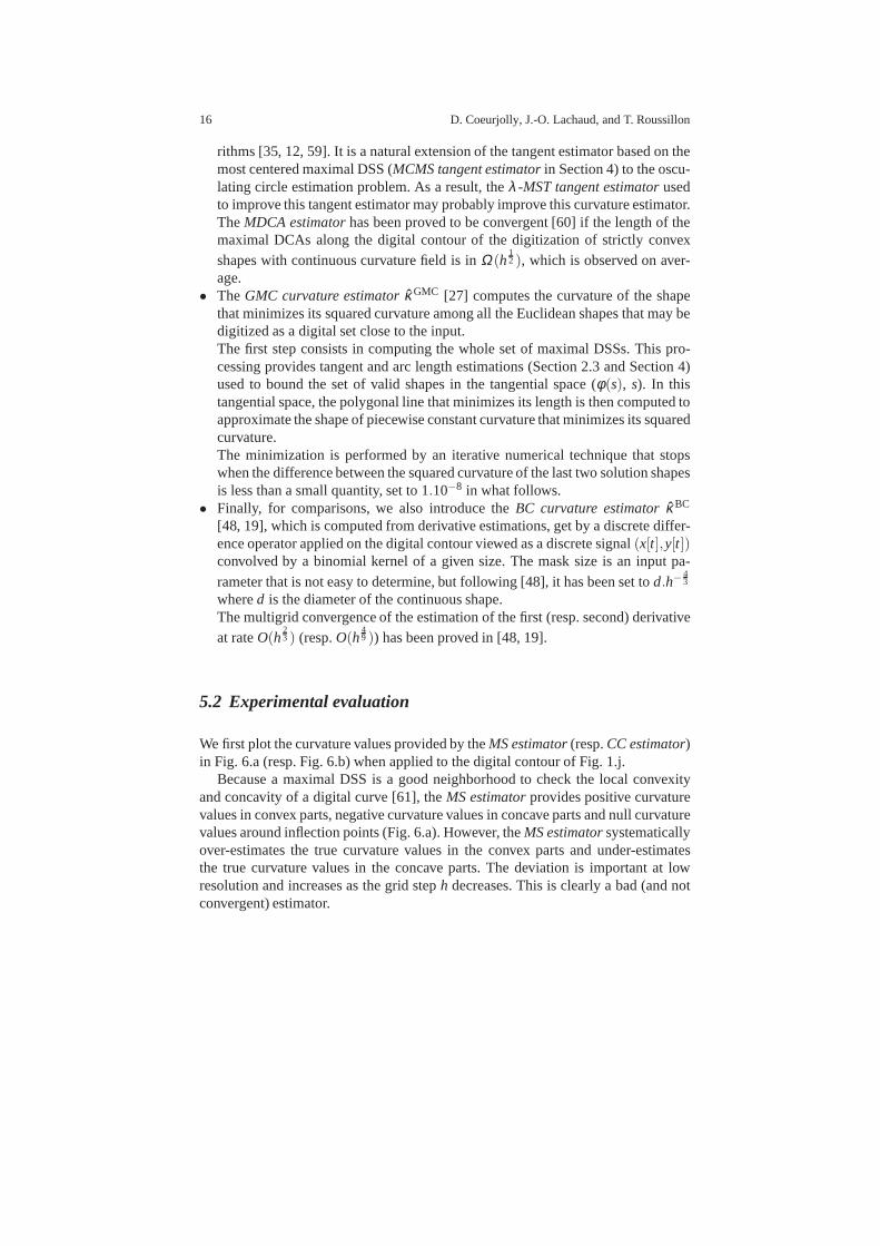
We first plot the curvature values provided by theMS estimator(resp.CC estimator)in Fig. 6.a (resp. Fig. 6.b) when applied to the digital contour of Fig. 1.j.

Because a maximal DSS is a good neighborhood to check the local convexityand concavity of a digital curve [61], theMS estimatorprovides positive curvaturevalues in convex parts, negative curvature values in concave parts and null curvaturevalues around inflection points (Fig. 6.a). However, theMS estimatorsystematicallyover-estimates the true curvature values in the convex parts and under-estimatesthe true curvature values in the concave parts. The deviation is important at lowresolution and increases as the grid steph decreases. This is clearly a bad (and notconvergent) estimator.


-0.6

-0.4

-0.2

0

0.2

0.4

0.6

0 200 400 600 800 1000 1200 1400

ground-truthMS

(a)

-0.6

-0.4

-0.2

0

0.2

0.4

0.6

0 200 400 600 800 1000 1200 1400

ground truthCC

(b)

Fig. 6 Curvature plots for the flower, digitized with a grid step equal to 0.1 (Fig. 1.j).MS estimatorin (a) andCC estimatorin (b).

The CC estimatordoes not respect the convex and concave parts of the digitalcontour (see the peak of positive curvature value near the starting point in Fig. 6.b),it oscillates a lot but gives correct results on average at low resolution.

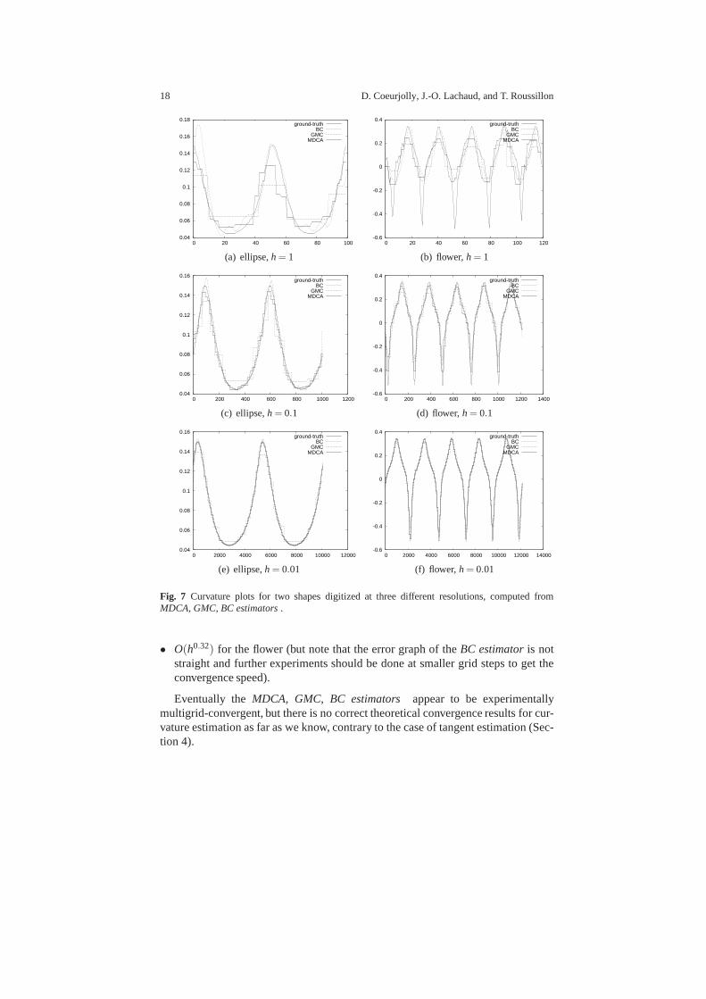
In Fig. 7, we compare the curvature plots derived from theMDCA, GMC, BCestimatorsto the ground-truth.

The visual deviation between the estimated graphs and the ground-truth graphreflects the average absolute error. For either estimator, the curvature estimationsare more accurate for the ellipse than for the flower. For either shape, the curvaturevalues get from any estimator get closer to the ground-truth(Fig. 7) and the absoluteerror decreases as the grid steph decreases.

For the ellipse and the flower, at grid steph= 0.01, theMDCA estimatorand theBC estimatorare better than theGMC estimator. In Fig. 7, their graphs are hardlyconfounded with the ground-truth graph.

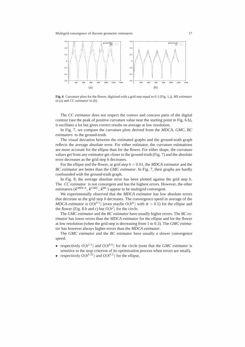
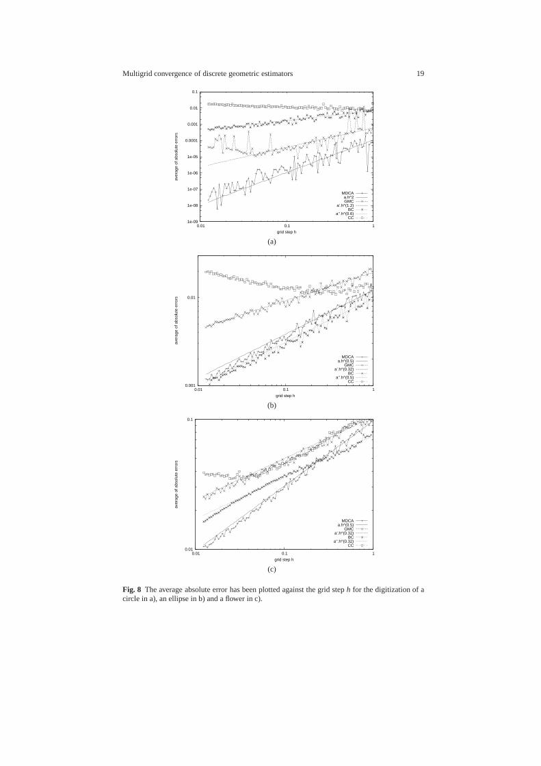
In Fig. 8, the average absolute error has been plotted against the grid steph.The CC estimatoris not convergent and has the highest errors. However, the otherestimators (κMDCA , κGMC, κBC) appear to be multigrid convergent.

We experimentally observed that theMDCA estimatorhas low absolute errorsthat decrease as the grid steph decreases. The convergence speed in average of theMDCA estimatoris O(h0.5) (even maybeO(hα) with α > 0.5) for the ellipse andthe flower (Fig. 8.b and c) butO(h2) for the circle.

TheGMC estimatorand theBC estimatorhave usually higher errors. TheBC es-timatorhas lower errors than theMDCA estimatorfor the ellipse and for the flowerat low resolution (when the grid step is decreasing from 1 to 0.3). TheGMC estima-tor has however always higher errors than theMDCA estimator.

The GMC estimatorand theBC estimatorhave usually a slower convergencespeed:

• respectivelyO(h1.2) andO(h0.6) for the circle (note that theGMC estimatorissensitive to the stop criterion of its optimization processwhen errors are small),

• respectivelyO(h0.32) andO(h0.5) for the ellipse,


0.04

0.06

0.08

0.1

0.12

0.14

0.16

0.18

0 20 40 60 80 100

ground-truthBC

GMCMDCA

(a) ellipse,h= 1

-0.6

-0.4

-0.2

0

0.2

0.4

0 20 40 60 80 100 120

ground-truthBC

GMCMDCA

(b) flower,h= 1

0.04

0.06

0.08

0.1

0.12

0.14

0.16

0 200 400 600 800 1000 1200

ground-truthBC

GMCMDCA

(c) ellipse,h= 0.1

-0.6

-0.4

-0.2

0

0.2

0.4

0 200 400 600 800 1000 1200 1400

ground-truthBC

GMCMDCA

(d) flower,h= 0.1

0.04

0.06

0.08

0.1

0.12

0.14

0.16

0 2000 4000 6000 8000 10000 12000

ground-truthBC

GMCMDCA

(e) ellipse,h= 0.01

-0.6

-0.4

-0.2

0

0.2

0.4

0 2000 4000 6000 8000 10000 12000 14000

ground-truthBC

GMCMDCA

(f) flower, h= 0.01

Fig. 7 Curvature plots for two shapes digitized at three differentresolutions, computed fromMDCA, GMC, BC estimators.

• O(h0.32) for the flower (but note that the error graph of theBC estimatoris notstraight and further experiments should be done at smaller grid steps to get theconvergence speed).

Eventually theMDCA, GMC, BC estimators appear to be experimentallymultigrid-convergent, but there is no correct theoreticalconvergence results for cur-vature estimation as far as we know, contrary to the case of tangent estimation (Sec-tion 4).


1e-09

1e-08

1e-07

1e-06

1e-05

0.0001

0.001

0.01

0.1

0.01 0.1 1

aver

age

of a

bsol

ute

erro

rs

grid step h

MDCAa.h^2GMC

a’.h^(1.2)BC

a’’.h^(0.6)CC

(a)

0.001

0.01

0.01 0.1 1

aver

age

of a

bsol

ute

erro

rs

grid step h

MDCAa.h^(0.5)

GMCa’.h^(0.32)

BCa’’.h^(0.5)

CC

(b)

0.01

0.1

0.01 0.1 1

aver

age

of a

bsol

ute

erro

rs

grid step h

MDCAa.h^(0.5)

GMCa’.h^(0.32)

BCa’’.h^(0.32)

CC

(c)

Fig. 8 The average absolute error has been plotted against the gridsteph for the digitization of acircle in a), an ellipse in b) and a flower in c).


6 Implementation

In this section, we discuss about implementation details ofboth the geometrical es-timators presented in the previous sections, and the experimental evaluation frame-work. All the estimators described in this chapter have beenimplemented in DGtal[1]. DGtal is an open-source C++ library focusing on the implementation of digitalgeometry objects and concepts. For short, it allows to represent images and objectsin n−dimensional digital spaces equipped with both geometricaland topologicaltools.

In the context of this chapter, we will only consider the representation and theanalysis of shape in dimension 2. As discussed in the introduction, the input dig-ital object can be obtained either from an explicit description, from a segmenta-tion process of an image (iso-level,. . . ), or as the digitization D(X,h) of a con-tinuous shapeX ∈ X. For the first two cases, DGtal provides mechanisms to con-struct such digital sets either explicitly or from a contourtracking process. For thelast case, DGtal implements various implicit and parametric continuous shapes forwhich some global and local geometrical quantities are known. All such shape im-plementations are model of a concept ofCEuclideanShapes1 (see Fig. 1 foran illustration of DGtal Euclidean shapes). A digital object is thus obtained froma GaussDigitizer parametrized by a model ofCEuclideanShapes and agrid steph. CEuclideanShapes models will be crucial for multigrid conver-gence analyses.

As discussed above and whatever the way the input digital object is specified, weneed to access to its geometrical information in various ways:

• As a sequence of grid points, subset ofZ2, e.g.for area and moment descriptors;• As a representation of its boundary,e.g.for tangent or curvature estimators.

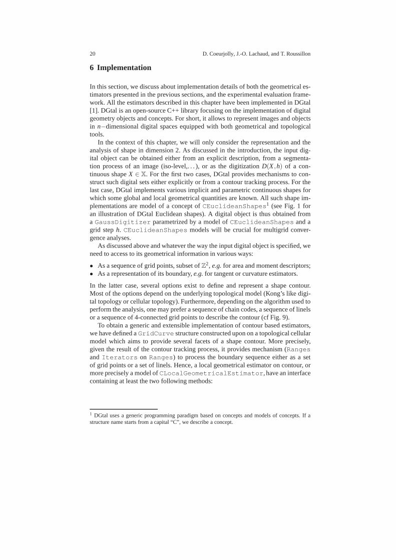
In the latter case, several options exist to define and represent a shape contour.Most of the options depend on the underlying topological model (Kong’s like digi-tal topology or cellular topology). Furthermore, depending on the algorithm used toperform the analysis, one may prefer a sequence of chain codes, a sequence of linelsor a sequence of 4-connected grid points to describe the contour (cf Fig. 9).

To obtain a generic and extensible implementation of contour based estimators,we have defined aGridCurve structure constructed upon on a topological cellularmodel which aims to provide several facets of a shape contour. More precisely,given the result of the contour tracking process, it provides mechanism (RangesandIterators on Ranges) to process the boundary sequence either as a setof grid points or a set of linels. Hence, a local geometrical estimator on contour, ormore precisely a model ofCLocalGeometricalEstimator, have an interfacecontaining at least the two following methods:

1 DGtal uses a generic programming paradigm based on conceptsand models of concepts. If astructure name starts from a capital “C”, we describe a concept.


(a) (b) (c) (d)

Fig. 9 Different representations of an Euclidean shape digitization: as a set of pixels(a), as asequence of 4-connected pixels(b), as a sequence of 1-cell orlinels (c) , as a sequence of gridpoint displacements(d).

• void init(double h, ConstIterator & begin,ConstIterator & end,...): initialize the geometrical estimatorwith grid steph on a contour defined between iteratorsbegin andend;

• Quantity eval( ConstIterator & it): evaluate the estimator at thepositionit of the contour and return aQuantity.

In our framework, the typeConstIterator is a template parameter chosen inthe contour iterator types provided inGridCurve.

Similarly, we have a concept ofCGlobalGeometricalEstimator andmodels of this concept have aneval() method which returns a unique quantityfor a shape (or subset of it).

Based on models of CEuclideanShapes, we can obtain ex-pected continuous values usingTrueLocalEstimatorOnPoints andTrueGlobalEstimatorOnPoints. Since both expected and estimatedvalues are given by estimators with a consistent interface,it makes themultigrid comparison very simple. Indeed, it allows to design a genericCompareLocalEstimators which return a statistic on the difference oftwo estimator values.

In the following example, we illustrate the mutligrid euclidean shape construc-tion and the comparison of three length estimators (RosenProffitt, DSS and MLP).In this example, we have detailed the overall process: shapeconstruction and dig-itization, domain and Khalimsky space construction, contour tracking and finally,evaluation of estimators.

/ / . . . ./ / h and r a d i u s are parameters here/ / . . . ./ / Typest ypedef Bal l2D<Space> Shape ;t ypedef Space : : P o i n t P o i n t ;t ypedef Space : : R ea l P o i n t R ea l P o i n t ;t ypedef Space : : I n t e g e r I n t e g e r ;t ypedef HyperRectDomain<Space> Domain ;t ypedef KhalimskySpaceND<Space : : d imens ion , I n t eg e r> KSpace ;t ypedef KSpace : : SCel l SCel l ;t ypedef GridCurve<KSpace>:: Po in t sRange Po in tsRange ;t ypedef GridCurve<KSpace>::ArrowsRange ArrowsRange ;t ypedef Po in tsRange : : C o n s t I t e r a t o r C o n s t I t e r a t o r O n P o i n t s ;

/ / Eu c l i d ea n b a l lShape aShape ( P o i n t ( 0 ,0 ) , r a d i u s ) ;


/ / Gauss D i g i t i z a t i o nG au s s D i g i t i ze r<Space , Shape> d ig ;d ig . a t t a c h ( aShape ) ;/ / a t t a c h e s t h e shape .d ig . i n i t ( aShape . getLowerBound ( ) , aShape . getUpperbound ( ) , h ) ;

/ / The domain s i z e i s g i ven by t h e d i g i t i z e r a cco r d i n g t o/ / t h e window and t h e s t e p .Domain domain = d ig . getDomain ( ) ;

/ / C rea te c e l l u l a r spaceKSpace K;

boo l ok = K. i n i t ( d ig . getLowerBound ( ) , d ig . getUpperBound ( ) ,t rue ) ;i f ( ! ok )

s t d : : c e r r<< ” ”<< ” e r r o r i n c r e a t i n g KSpace . ”<< s t d : : en d l ;

re turn f a l s e ;

t ry

/ / E x t r a c t s shape boundaryS u r f e l A d j acen cy<KSpace : : d imens ion> SAdj ( t rue ) ;SCel l b e l = S u r f aces<KSpace>:: f i ndABel ( K, dig , 10000 ) ;

/ / G e t t i n g t h e c o n s e c u t i v e s u r f e l s o f t h e 2D boundarys t d : : v ec t o r<Po in t> p o i n t s ;S u r f aces<KSpace>:: t r ack 2 D B o u nda r yP o in t s ( p o i n t s ,

K, SAdj ,d ig , b e l ) ;

t r a c e . i n f o ( )<< ” # t r a c k i n g . . . ”<< en d l ;

/ / C rea te GridCurveGridCurve<KSpace> g r i d c u r v e ;g r i d c u r v e . i n i t F r o mV ec t o r ( p o i n t s ) ;t r a c e . i n f o ( )<< ” # g r i d curve c r ea t ed , h=” << h<< en d l ;

/ / rangesArrowsRange r a = g r i d c u r v e . getArrowsRange ( ) ;Po in t sRange rp = g r i d c u r v e . g e t P o i n t s R an g e ( ) ;

/ / Th ree l e n g t h e s t i m a t o r s work ing on d i f f e r e n t co n t o u r/ / r e p r e s e n t a t i o n s

R o s en P r o f f i t t Lo ca l L en g t h E s t i m a t o r< ArrowsRange : : C o n s t I t e r a t o r> R o s e n P r o f f i t t l e n g t h ;R o s e n P r o f f i t t l e n g t h . i n i t ( h , r a . beg in ( ) , r a . end ( ) , g r i dc u r v e . i s C l o s ed ( ) ) ;

DSSLeng thEst imato r< Po in tsRange : : C o n s t I t e r a t o r> DSSlength ;DSSlength . i n i t ( h , rp . beg in ( ) , rp . end ( ) , g r i d c u r v e . i s C lo s ed ( ) ) ;

MLPLengthEst imator< Po in tsRange : : C o n s t I t e r a t o r> MLPlength ;MLPlength . i n i t ( h , rp . beg in ( ) , rp . end ( ) , g r i d c u r v e . i s C lo s ed ( ) ) ;

t r a c e . i n f o ( )<< ” # Es t i ma t i o n s ”<<s t d : : en d l ;t r a c e . i n f o ( )<< ” #h t r u e R o s e n P r o f f i t t DSS MLP ” <<s t d : : en d l ;t r a c e . i n f o ( )<< h << ” ” << M PI∗2.0

<< ” ” << R o s e n P r o f f i t t l e n g t h . ev a l ( )<< ” ” << DSSlength . ev a l ( )<< ” ” << MLPlength . ev a l ( )<< s t d : : en d l ;

ca tch ( I n p u t Ex cep t i o n e )

s t d : : c e r r<< ” ”<< ” e r r o r i n f i n d i n g a b e l . ” << s t d : : en d l ;

re turn f a l s e ;

7 Related problems and perspectives

7.1 Geometric estimators along damaged or noisy contours

In real applications, images may have been damaged or acquisition devices mayinduce noise in the image data. Furthermore, binarization algorithms and segmen-tation algorithms may also damage the boundary of the regions or shapes. These


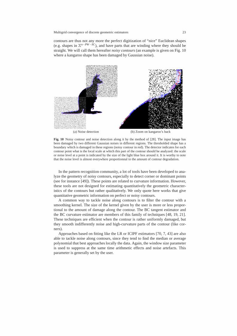
contours are thus not any more the perfect digitization of “nice” Euclidean shapes(e.g. shapes inXn−PW−SC), and have parts that are winding where they should bestraight. We will call them hereafternoisy contours(an example is given on Fig. 10where a kangaroo shape has been damaged by Gaussian noise).

(a) Noise detection (b) Zoom on kangaroo’s back

Fig. 10 Noisy contour and noise detection along it by the method of [28]. The input image hasbeen damaged by two different Gaussian noises in different regions. The thresholded shape has aboundary which is damaged in these regions (noisy contour inred). The detector indicates for eachcontour point what is the local scale at which this part of thecontour should be analyzed: the scaleor noise level at a point is indicated by the size of the light blue box around it. It is worthy to notethat the noise level is almost everywhere proportionnal to the amount of contour degradation.

In the pattern recognition community, a lot of tools have been developed to ana-lyze the geometry of noisy contours, especially to detect corner or dominant points(see for instance [49]). These points are related to curvature information. However,these tools are not designed for estimating quantitativelythe geometric character-istics of the contours but rather qualitatively. We only quote here works that givequantitative geometric information on perfect or noisy contours.

A common way to tackle noise along contours is to filter the contour with asmoothing kernel. The size of the kernel given by the user is more or less propor-tional to the amount of damage along the contour. The BC tangent estimator andthe BC curvature estimator are members of this family of techniques [48, 19, 21].These techniques are efficient when the contour is rather uniformly damaged, butthey smooth indifferently noise and high-curvature parts of the contour (like cor-ners).

Approaches based on fitting like the LR or ICIPF estimators [70, 7, 43] are alsoable to tackle noise along contours, since they tend to find the median or averagepolynomial that best approaches locally the data. Again, the window size parameteris used to suppress at the same time arithmetic effects and noise artefacts. Thisparameter is generally set by the user.


In the digital geometry community, a common technique is to use the so-calledblurred segments[16] instead of digital straight segment. Compared to digitalstraight segment whose thickness is always less than 1, blurred segments have auser-given maximal thickness. The noisy parts of contours are thus ignored when us-ing a larger thickness. Several estimators just replace standard segments with blurredsegments so as to take into account noisy contours. For instance, the curvature esti-mator presented in [52] is the noisy variant of the CC estimator. The GMC estimatoralso uses blurred segments to handle noisy contours. The thickness is generally setby the user.

Note that digital estimators based on digital straight segments (like the H0-1GD,MCMS andλ -MST tangent estimators, or the MDCA curvature estimator) can alsobe adapted to noisy contours by subsampling the input contour. For instance, we canuse a 3×3 tile over the input contour so as to remove perturbation no greater than1 pixel along the contour. However we have yet not run a full set of experimentsso as to know if this approach leads to better estimators thanthe ones quoted in thepreceding paragraphs.

Finally, all these techniques require the determination ofone or several param-eters in order to process at best noisy contours. This scale or smoothing parametermust not be too low otherwise damaged parts are considered high-curvature placesor corners, but it must not be too high also in order to preserve features and to haveaccurate estimates of geometric information.

If a grey-level input noisy image is available, scale space analysis may provideinformation on the amount of noise [18, 31, 9, 24]. They cannot handle directlynoisy contours. For noisy contours, Kerautret and Lachaud [28] have recently pro-posed a method to automatically detect the meaningful scales of digital contours. Itcan give locally along the contour what it is the amount of noise and the first scale atwhich the contour should be analyzed (see Fig. 10, and onlinedemonstration [29]).Their technique relies on the asymptotic properties of maximal digital straight seg-ments. They have proposed a variant ofλ -MST estimator for noisy contours, whichuses the noise information given by the meaningful scales [30].

7.2 Geometric estimators in 3D and nD

In higher dimensions, several 2D estimators or frameworks can extended. However,many open problems exist and beside the fact that few multigrid-convergent proofsexist, a complete experimental multigrid evaluation of curvature estimators for in-stance has not been done yet on digital surfaces inZ3. In this section, we just give abrief overview of existing techniques:

• Surface area:to compute the area of a surface inZ3, a first solution is based onweighted local configurations [69, 45]. The idea is to associated weights to lo-cal configurations of surface voxels or surfels. Then, givenan object, the surfacearea is approximated by summing all weights associated to all configurations de-fined on the object surface. Similarly to the BLUE estimator,weights are given


by a statistical analysis to minimize surface area error fora given class of shapes.By deriving results from the length case in dimension 2 [63],surface weightedconfiguration estimators can never achieve multigrid convergence. In [47], theauthors use statistical analysis and integral geometry to design a fast estimationof the surface area. Again, the quality of the estimation is controlled by a param-eter (number of line probes). Another option is to generalize the discrete normalvector integration scheme as described in [10, 13]. As detailed in [11], we canprove that if the normal vector estimation is multigrid convergent, then the in-tegration of the vector field leading to the surface area estimation is multigridconvergent as well.

• Normal vector field computation: at a pointx on a smooth surface, the normalvector atx can be defined as the cross product of first order derivatives at x (tan-gent) of two curves lying on the surface crossing atx. In a digital context, given asurface element of a cellular representation of a digital surface, two natural digi-tal 4-connected curves can be defined by the intersection of the surface with thetwo axis planes containing the surfel elementary normal vector. Hence, Lenoiret al. suggested to compute the normal vector at a surfel as the cross productof tangent computed on the two 2D digital curves [41]. Following this frame-work, multigrid convergence can be achieved if the tangent estimator used on the2D curves is multigrid convergent [11, 36]. The normal vector field of a digitalsurface inZn, for arbitraryn, can be computed with a similar approach [37].

• Curvature: For curvature computation on digital surfaces, only few estimatorshave been proposed in the digital geometry framework. We cancite Lenoir’s slicebased approach for the mean curvature estimation [42], Gauss map area evalua-tion for the gaussian curvature [10], techniques based on integral invariants forboth mean and gaussian curvatures [6, 55, 54]. Integral invariant techniques aredefinitely relevant in the digital geometry context, even incase of noisy surface.However, they require a window parameter which could be difficult to set for alarge class of shapes.In the computational geometry field, several techniques have been proposed toconstruct accurate curvature estimators with bounded errors. Usually, bounds areparametrized by a sampling parameter for a given sampling hypothesis. An ex-ample of a sampling hypothesis for a smooth surface would be that the samplingdensity should be proportional to the curvature. In this context, convergence orstability of geometric estimators have been proposed as a function of the sam-pling parameter. In many situations the sampling theorems used in computationalgeometry do not match with the specific isotropic behavior ofdigital surfaces. In[3, 8, 51], estimators are defined on point sets based on Voronoi structures andthe error is given in terms of Hausdorff distance (which is consistent with digi-tal surfaces). Investigating the links between computational geometry and digitalgeometry on this subject is a challenging problem.


7.3 Current bottlenecks and open problems

As detailed in the previous sections, we can overview current theoretical bottlenecksin the design of discrete geometric estimators:

• Stability w.r.t. noise: Prior detection of the contour local noise level to be usedas an estimator parameter, or with estimator which are theoretically robust to agiven noise model.

• Estimators of differential quantity of order 2: In our point of view, existingcurvature estimators are not yet satisfactory since eitherno proof of multigridconvergence exists, or the convergence is controlled by an external parameter(windows size, Gaussian kernel width, . . . ). It would be interesting, for instance,to focus on the multigrid behavior of circular arc segment ondigital 2D contours.Indeed, many proofs related to the length or the tangent estimation are basedon the multigrid behavior of DSS. On digital surfaces and in higher dimension,we think that a better understanding of links between computational and digitalgeometry results would lead to new results in this domain.

Beside these theoretical bottlenecks, complete multigridexperimental evalua-tions are now mandatory when designing a new discrete estimator. With the help ofboth a theoretical methodology (multigrid shape database and error measures) andopensource libraries (ImaGene [2] or DGtal [1]), we expect to have a completeand stable experimental framework. An important future work would be to continuethe implementation of existing estimators with comparative studies. In dimension 3,main bottlenecks are related to efficiency and computational costs. Indeed, in manyMaterial sciences or Medical imaging applications, we may have to analyse digitalshapes whose size achieves up to 20483. In the implementation of 3D estimators,several theoretical and technical problems have to be addressed (out-of-core tech-niques, hierarchical data representation and adaptive algorithms, . . . ).

References

1. DGtal: Digital Geometry tools and algorithms library,http://liris.cnrs.fr/dgtal2. ImaGene: Generic digital image library,https://gforge.liris.cnrs.fr/

projects/imagene3. Amenta, N., Kil, Y.: Defining point-set surfaces. In: ACM SIGGRAPH. vol. 23, p. 270. ACM

(2004)4. Asano, T., Kawamura, Y., Klette, R., Obokata, K.: Minimum-length polygons in approxima-

tion sausages. In: 4th International Workshop on Visual Form. Lecture Notes in ComputerScience, vol. 2059, pp. 103–112. Springer-Verlag, Berlin (2001)

5. Brlek, S., Labelle, G., Lacasse, A.: The discrete green theorem and some applications in dis-crete geometry. Theoretical Computer Science 346(2-3), 200 – 225 (2005)

6. Bullard, J.W., Garboczi, E.J., Carter, W.C., Fullet, E.R.: Numerical methods for computinginterfacial mean curvature. Computational materials science 4, 103–116 (1995)

7. Cazals, F., Pouget, M.: Estimating differential quantities using polynomial fitting of osculatingjets. Computer Aided Geometric Design 22, 121–146 (2005)


8. Chazal, F., Cohen-Steiner, D., Lieutier, A., Thibert, B.: Stability of Curvature Measures (2008)9. Chen, K.: Adaptive smoothing via contextual and local discontinuities. IEEE Transactions on

Pattern Analysis and Machine Intelligence 27(10), 1552–1566 (2005)10. Coeurjolly, D.: Algorithmique et geometrie pour la caracterisation des courbes et des surfaces.

Ph.D. thesis, Universit Lyon 2 (2002)11. Coeurjolly, D., Flin, F., Teytaud, O., Tougne, L.: Multigrid convergence and surface area esti-

mation. In: Theoretical Foundations of Computer Vision ”Geometry, Morphology, and Com-putational Imaging”. pp. 101–119. No. 2616 in Lecture Notesin Computer Science, Springer-Verlag (2003)

12. Coeurjolly, D., Gerard, Y., Reveilles, J.P., Tougne,L.: An elementary algorithm for digital arcsegmentation. Discrete Applied Mathematics 139(1-3), 31–50 (2004)

13. Coeurjolly, D., Klette, R.: A comparative evaluation oflength estimators of digital curves.IEEE Transactions on Pattern Analysis and Machine Intelligence 26(2), 252–258 (2004)

14. Coeurjolly, D., Miguet, S., Tougne, L.: Discrete curvature based on osculating circle estima-tion. In: 4th International Workshop on Visual Form, Lecture Notes in Computer Science, vol.2059, pp. 303–312 (2001)

15. Coeurjolly, D., Svensson, S.: Estimation of curvature along curves with application to fibresin 3d images of paper. In: 13th Scandinavian Conference on Image Analysis, Lecture Notes inComputer Science, vol. 2749, pp. 247–254 (2003)

16. Debled-Rennesson, I., Feschet, F., Rouyer-Degli, J.: Optimal blurred segments decompositionof noisy shapes in linear times. Computers and Graphics 30, 30–36 (2006)

17. Dorst, L., Smeulders, A.W.M.: Length estimators for digitized contours. Computer Vision,Graphics and Image Processing 40(3), 311–333 (1987)

18. Elder, J., Zucker, S.W.: Local scale control for edge detection and blur estimation. IEEE Trans-actions on Pattern Analysis and Machine Intelligence 20(7), 669–716 (1998)

19. Esbelin, H.A., Malgouyres, R.: Convergence of binomial-based derivative estimation for c2-noisy discretized curves. In: 15th Discrete Geometry for Computer Imagery, Lecture Notes inComputer Science, vol. 5810, pp. 57–66 (2009)

20. Feschet, F., Tougne, L.: Optimal time computation of thetangent of a discrete curve: Applica-tion to the curvature. In: Proc. 8th Discrete Geometry for Computer Imagery. pp. 31–40. No.1568 in Lecture Notes in Computer Science (1999)

21. Fiorio, C., Mercat, C., Rieux, F.: Curvature estimationfor discrete curves based on auto-adaptive masks of convolution. In: Computational Modelingof Objects Presented in Images,Lecture Notes in Computer Science, vol. 6026, pp. 47–59 (2010)

22. Fleischmann, O., Wietzke, L., Sommer, G.: A novel curvature estimator for digital curvesand images. In: 32th Annual Symposium of the German Association for Pattern Recognition,Lecture Notes in Computer Science, vol. 6376, pp. 442–451 (2010)

23. Gerard, Y., Provot, L., Feschet, F.: Introduction to digital level layers. In: 16th IAPR Inter-national Conference Discrete Geometry for Computer Imagery. Lecture Notes in ComputerScience, vol. 6607, pp. 83–94. Springer (2011)

24. Goshtasby, A., Satter, M.: An adaptive window mechanismfor image smoothing. ComputerVision and Image Understanding 111, 155–169 (2008)

25. Hermann, S., Klette, R.: A comparative study on 2d curvature estimators. In: 17th InternationalConference on Computer Theory and Applications. pp. 584–589 (2007)

26. Huxley, M.N.: Exponential sums and lattice points. Proceedings London Mathematical Soci-ety 60, 471–502 (1990)

27. Kerautret, B., Lachaud, J.O.: Curvature estimation along noisy digital contours by approxi-mate global optimization. Pattern Recognition 42(10), 2265–2278 (2009)

28. Kerautret, B., Lachaud, J.: Multiscale Analysis of Discrete Contours for Unsupervised NoiseDetection. In: 13th International Workshop on Combinatorial Image Analysis. Lecture Notesin Computer Science, vol. 5852, pp. 187–200. Springer, Mexico Mexique (2009)

29. Kerautret, B., Lachaud, J.O.: Noise level and meaningful scale detection online demonstration.http://kerrecherche.iutsd.uhp-nancy.fr/MeaningfulBoxes (2010)


30. Kerautret, B., Lachaud, J.: Meaningful scales detection along digital contours for unsuper-vised local noise estimation. IEEE Transactions on PatternAnalysis and Machine Intelligence(Submitted)

31. Kervrann, C.: An adaptive window approach for image smoothing and structures preserving.In: 8th European Conference on Computer Vision. Lecture Notes in Computer Science, vol.3023, pp. 132–144. Springer (2004)

32. Klette, R., Rosenfeld, A.: Digital Geometry - GeometricMethods for Digital Picture Analysis(2004)

33. Klette, R.,Zunic, J.: Multigrid convergence of calculated features in image analysis. Journalof Mathematical Imaging and Vision 13, 173–191 (2000)

34. Kovalevsky, V., Fuchs, S.: Theoretical and experimental analysis of the accuracy of perimeterestimates. In: Proceedings Robust Computer Vision. pp. 218–242 (1992)

35. Kovalevsky, V.A.: New definition and fast recognition ofdigital straight segments and arcs. In:10th International Conference on Pattern Analysis and Pattern Recognition. pp. 31–34 (1990)

36. Lachaud, J.O.: Espaces non-euclidiens et analyse d’image : modeles deformables riemannienset discrets, topologie et geometrie discrete. Habilitation diriger des recherches, UniversiteBordeaux 1, Talence, France (2006), (en francais)

37. Lachaud, J.O., Vialard, A.: Geometric measures on arbitrary dimensional digital surfaces. In:11th International Conference Discrete Geometry for Computer Imagery. Lecture Notes inComputer Science, vol. 2886, pp. 434–443. Springer (2003)

38. Lachaud, J.O., Vialard, A., de Vieilleville, F.: Analysis and comparative evaluation of discretetangent estimators. In: 12th International Conference on Discrete Geometry for ComputerImagery. Lecture Notes in Computer Science, vol. 3429, pp. 140–251. Springer (2005)

39. Lachaud, J.O., Vialard, A., de Vieilleville, F.: Fast, accurate and convergent tangent estimationon digital contours. Image and Vision Computing 25(10), 1572–1587 (2007)

40. Latecki, L.J., Conrad, C., Gross, A.: Preserving topology by a digitization process. Journal ofMathematical Imaging and Vision 8(2), 131–159 (1998)

41. Lenoir, A., Malgouyres, R., Revenu, M.: Fast computation of the normal vector field of thesurface of a 3d discrete object. In: 6th International Workshop on Discrete Geometry for Com-puter Imagery. vol. 1176, pp. 101–109 (1996)

42. Lenoir, A.: Fast estimation of mean curvature on the surface of a 3d discrete object. In: 7thInternational Workshop on Discrete Geometry for Computer Imagery. pp. 175–186. Springer-Verlag (1997)

43. Lewiner, T., Gomes Jr., J.D., Lopes, H., Craizer, M.: Curvature and torsion estimators basedon parametric curve fitting. Computers & Graphics 29, 641–655 (2005)

44. Lien, S.L.C.: Combining Computation with Geometry. Ph.D. thesis, California Institute ofTechnology (1984)

45. Lindblad, J.: Surface area estimation of digitized 3D objects using weighted local configura-tions. Image and Vision Computing 23(2), 111–122 (2005)

46. Liu, H., Latecki, L., Liu, W.: A unified curvature definition for regular, polygonal, and digitalplanar curves. International Journal of Computer Vision 80(1), 104–124 (2008)

47. Liu, Y.S., Yi, J., Zhang, H., Zheng, G.Q., Paul, J.C.: Surface area estimation of digitized 3dobjects using quasi-Monte Carlo methods. Pattern Recognition 43(11), 3900–3909 (2010)

48. Malgouyres, R., Brunet, F., Fourey, S.: Binomial convolutions and derivatives estimation fromnoisy discretizations. In: 14th Discrete Geometry for Computer Imagery, Lecture Notes inComputer Science, vol. 4992, pp. 370–379 (2008)

49. Marji, M.: On the detection of dominant points on digitalplanar curves. Ph.D. thesis, WayneState University, Detroit, Michigan (2003)

50. Matas, J., Shao, Z., Kittler, J.: Estimation of curvature and tangent direction by median fil-tered differencing. In: 8th International Conference on Image Analysis and Processing, Lec-ture Notes in Computer Science, vol. 974, pp. 83–88 (1995)

51. Merigot, Q., Ovsjanikov, M., Guibas, L.: Robust Voronoi-based Curvature and Feature Esti-mation. In: SIAM/ACM Joint Conference on Geometric and Physical Modeling (2009)


52. Nguyen, T., Debled-Rennesson, I.: Curvature estimation in noisy curves. In: 12th Interna-tional Conference on Computer Analysis of Images and Patterns, Lecture Notes in ComputerScience, vol. 4673, pp. 474–481 (2007)

53. Novotni, M., Klein, R.: Shape retrieval using 3D zernikedescriptors. Computer-Aided Design36(11), 1047–1062 (2004)

54. Pottmann, H., Wallner, J., Huang, Q., Yang, Y.: Integralinvariants for robust geometry pro-cessing. Computer Aided Geometric Design 26(1), 37–60 (2009)

55. Pottmann, H., Wallner, J., Yang, Y., Lai, Y., Hu, S.: Principal curvatures from the integralinvariant viewpoint. Computer Aided Geometric Design 24(8-9), 428–442 (2007)

56. Proffitt, D., Rosen, D.: Metrication errors and coding efficiency of chain-encoding schemesfor the representation of lines and edges. Computer Graphics and Image Processing 10(4),318 – 332 (1979)

57. Provencal, X., Lachaud, J.O.: Two linear-time algorithms for computing the minimum lengthpolygon of a digital contour. In: 11-th Internation Conference on Discrete Geometry for Com-puter Imagery. Lecture Notes in Computer Science, vol. 5810, pp. 104–117 (2009)

58. Provot, L., Gerard, Y.: Estimation of the derivatives of a digital function with a convergentbounded error. In: 16th IAPR International Conference in Discrete Geometry for ComputerImagery. Lecture Notes in Computer Science, vol. 6607, pp. 284–295. Springer (2011)

59. Roussillon, T., Sivignon, I., Tougne, L.: On three constrained versions of the digital circulararc recognition problem. In: 15th IAPR International Conference on Discrete Geometry forComputer Imagery. Lecture Notes in Computer Science (2009)

60. Roussillon, T., Lachaud, J.O.: Accurate curvature estimation along digital contours with max-imal digital circular arcs. In: 14th International Workshop in Combinatorial Image Analysis.Lecture Notes in Computer Science, vol. 6636, pp. 43–55. Springer (2011)

61. Roussillon, T., Sivignon, I.: Faithful polygonal representation of the convex and concave partsof a digital curve. Pattern Recognition 44(10-11), 2693 – 2700 (2011)

62. Sloboda, F., Zatko, B., Stoer, J.: On approximation of planar one-dimensional continua. In:Advances in Digital and Computational Geometry. pp. 113–160 (1998)

63. Tajine, M., Daurat, A.: On local definitions of length of digital curves. In: 11-th InternationConference on Discrete Geometry for Computer Imagery, Lecture Notes in Computer Science,vol. 2886, pp. 114–123. Springer Berlin, Heidelberg (2003)

64. Teague, M.R.: Image analysis via the general theory of moments. Journal of the Optical Soci-ety of America 70(8), 920–930 (1980)

65. Vialard, A.: Geometrical parameters extraction from discrete paths. In: 7th Discrete Geometryfor Computer Imagery, Lecture Notes in Computer Science, vol. 1176, pp. 24–35 (1996)

66. de Vieilleville, F., Lachaud, J.O.: Experimental comparison of continuous and discrete tan-gent estimators along digital curves. In: 12th International Workshop on Combinatorial ImageAnalysis. Lecture Notes in Computer Science, vol. 4958, pp.26–37. Springer (2008)

67. de Vieilleville, F., Lachaud, J.O.: Comparison and improvement of tangent estimators on dig-ital curves. Pattern Recognition 42(8), 1693–1707 (2009)

68. de Vieilleville, F., Lachaud, J.O., Feschet, F.: Convexdigital polygons, maximal digital straightsegments and convergence of discrete geometric estimators. Journal of Mathematical Imagingand Vision 27(2), 139–156 (2007)

69. Windreich, G., Kiryati, N., Lohmann, G.: Voxel-based surface area estimation: from theory topractice. Pattern Recognition 36(11), 2531–2541 (2003)

70. Worring, M., Smeulders, A.W.M.: Digital curvature estimation. CVGIP: Image Understanding58(3), 366–382 (1993)

Multigrid convergence of discrete geometric estimators this chapter, we use DGtal to represent...

Documents

Transcript of Multigrid convergence of discrete geometric estimators this chapter, we use DGtal to represent...