
On Computing Geometric Estimators of Locationcgm.cs.mcgill.ca/~athens/Papers/G_A_thesis.pdf · le...
71
On Computing Geometric Estimators of Location Greg Aloupis School of Computer Science McGill University Montreal, Canada March 2001 A thesis submitted to the Faculty of Graduate Studies and Research in partial fulfillment of the requirements for the degree of Master of Science Copyright c 2001 Greg Aloupis
Transcript of On Computing Geometric Estimators of Locationcgm.cs.mcgill.ca/~athens/Papers/G_A_thesis.pdf · le...

On Computing Geometric Estimators of Location
Greg Aloupis
School of Computer Science
McGill University
Montreal, Canada
March 2001
A thesis submitted to the
Faculty of Graduate Studies and Research
in partial fulfillment of the requirements for
the degree of Master of Science
Copyright c©2001 Greg Aloupis

Abstract
Let S be a data set of n points in Rd, and µ be a point in Rd which “best” describes
S. Since the term “best” is subjective, there exist several definitions for finding µ.
However, it is generally agreed that such a definition, or estimator of location, should
have certain statistical properties which make it robust. Most estimators of location
assign a depth value to any point in Rd and define µ to be a point with maximum
depth. Here, new results are presented concerning the computational complexity
of estimators of location. We prove that in R2 the computation of simplicial and
halfspace depth of a point requires Ω(n log n) time, which matches the upper bound
complexities of algorithms by Rousseeuw and Ruts. Our lower bounds also apply to
two sign tests, that of Hodges and that of Oja and Nyblom. In addition, we propose
algorithms which reduce the time complexity of calculating the points with greatest
Oja and simplicial depth. Our fastest algorithms use O(n3 log n) and O(n4) time
respectively, compared to the algorithms of Rousseeuw and Ruts which use O(n5 log n)
time. One of our algorithms may also be used to find a point with minimum weighted
sum of distances to a set of n lines in O(n2) time. This point is called the Fermat-
Torricelli point of n lines by Roy Barbara, whose algorithm uses O(n3) time. Finally,
we propose a new estimator which arises from the notion of hyperplane depth recently
defined by Rousseeuw and Hubert.
ii

Resume
Que S soıt un ensemble de n points en Rd, et que µ soıt un point en Rd qui decrit
S le mieux. Comme le terme “mieux” est subjectif, il existe plusieurs definitions
pour trouver µ. Cependent, il est generalement convenu qu’une telle definition, ou
estimateur d’emplacement, devrait avoir certaines proprietes statistiques qui la fait
robuste. La plupart des estimateurs d’emplacement assignent une valeur de pro-
fondeur a n’importe quel point en Rd et ils definissent µ comme un point avec une
profondeur maximum. Ici, de nouveaux resultats sont presentes concernant la com-
plexite informatique d’estimateurs d’emplacement. Nous prouvons qu’en R2 le calcul
de la profondeur simpliciale et halfspace d’un point necessite un temps Ω(n log n), qui
egale aux bornes superieures des complexites des algorithmes par Rousseeus et Ruts.
Nos bornes inferieures s’appliquent aussi a deux sign tests, celui de Hodges et celui
d’Oja et Nyblom. De plus, nous proposons des algorithmes qui reduisent le temps in-
formatique de calculer les points avec la meilleure profondeur Oja et simpliciale. Nos
algorithmes les plus rapides utilisent le temps O(n3 log n) et O(n4) respectivement,
compares aux algorithmes de Rousseeuw et Ruts qui utilisent le temps O(n5 log n).
Un de nos algorithmes pourrait etre utilise pour trouver un point avec une somme
minimum de distances d’un ensemble de n lignes en temps O(n2). Ce point est nomme
le point Fermat–Torricelli de n lignes par Roy Barbara, dont l’algorithme utilise le
temps O(n3). Enfin, nous proposons un nouveau estimateur, qui surgit de la notion
de profondeur hyperplane recement defini par Rousseeuw et Hubert.
iii

Statement of Originality
Except for the introduction, the appendix, and results whose authors have been cited
where first introduced, all elements of this thesis are original contributions to knowl-
edge. Assistance has been received only where mentioned in the acknowledgements.
iv

Acknowledgements
I would like to thank my supervisor, Dr. Godfried Toussaint, for introducing me
to the field of computational geometry. It was through his graduate courses that I
initially became interested in this field. He has always been willing to spend time
discussing interesting problems. This thesis was born from a project that he suggested
to me for his course in pattern recognition. I am honored to have been a research
assistant for Dr. Toussaint and Dr. David Avis, and I am grateful for their funding,
which allowed me to devote my time to research.
While working on this thesis, I received a great amount of help from Dr. Toussaint
and from Mike Soss. Despite their busy schedule, they were always willing to give me
advice. The three of us worked together to obtain the results presented in chapter
4. These results also appear in the form of a technical report [AST01]. We worked
together with Carmen Cortes and Paco Gomez to obtain the results presented in
chapter 3, which may also be found in [ACG+01].
I thank my family in Greece for always encouraging me, and my family in Canada
for giving me a home away from home. I am also extremely fortunate to have met
Erin, who made the past few years of hard work bearable.
Finally, none of this would have been possible without the support of my parents,
Yvonne and Nick, to whom I dedicate this thesis.
v

Contents
Abstract ii
Resume iii
Statement of Originality iv
Acknowledgements v
1 Introduction 1
2 Multivariate Medians 9
2.1 The L1 Median . . . . . . . . . . . . . . . . . . . . . . . . . . . . . . 9
2.2 The Halfspace Median . . . . . . . . . . . . . . . . . . . . . . . . . . 11
2.3 Convex Hull Peeling and Related Methods . . . . . . . . . . . . . . . 14
2.4 The Oja Simplex Median . . . . . . . . . . . . . . . . . . . . . . . . . 16
2.5 The Simplicial Median . . . . . . . . . . . . . . . . . . . . . . . . . . 17
2.6 Hyperplane Depth and a New Median . . . . . . . . . . . . . . . . . . 20
3 Algorithms and Lower Bounds for Depth in R2 23
3.1 Algorithms for the Depth of a Point in R2 . . . . . . . . . . . . . . . 23
3.1.1 Halfspace Depth Calculation . . . . . . . . . . . . . . . . . . . 23
3.1.2 Simplicial Depth Calculation . . . . . . . . . . . . . . . . . . . 25
vi
vii
3.2 Lower Bounds for Computing the Depth of a Point in R2 . . . . . . . 26
3.2.1 Halfspace Depth Lower Bound . . . . . . . . . . . . . . . . . . 26
3.2.2 Simplicial Depth Lower Bound . . . . . . . . . . . . . . . . . . 29
3.3 Ramifications . . . . . . . . . . . . . . . . . . . . . . . . . . . . . . . 30
3.3.1 The Bivariate Hodges Sign Test . . . . . . . . . . . . . . . . . 30
3.3.2 The Bivariate Oja-Nyblom Sign Test . . . . . . . . . . . . . . 31
4 New Median Algorithms 33
4.1 Oja Median Algorithms . . . . . . . . . . . . . . . . . . . . . . . . . . 33
4.1.1 Properties of the Oja Median in R2 . . . . . . . . . . . . . . . 33
4.1.2 The two Algorithms . . . . . . . . . . . . . . . . . . . . . . . 39
4.1.3 The Fermat-Torricelli Points of n Lines . . . . . . . . . . . . . 42
4.2 Simplicial Median Algorithm . . . . . . . . . . . . . . . . . . . . . . . 42
5 Conclusion 48
A Arrangements of Lines 50

List of Figures
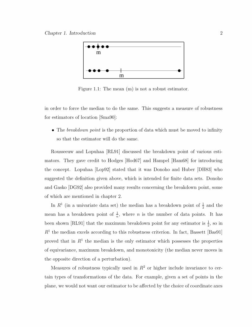
1.1 The mean (m) is not a robust estimator. . . . . . . . . . . . . . . . . 2
2.1 The breakdown point of the L1 median is 12. . . . . . . . . . . . . . . 11
2.2 The halfspace depth of some points. . . . . . . . . . . . . . . . . . . . 12
2.3 Multivariate median (m) via convex hull peeling. . . . . . . . . . . . . 14
2.4 Example of how the breakdown point of convex hull peeling can be
made to approach zero. . . . . . . . . . . . . . . . . . . . . . . . . . . 15
2.5 The simplices considered for a candidate Oja median (θ) in R2. (n = 4) 16
2.6 The simplices considered for the simplicial median in R2. (n = 4) . . 18
2.7 Data splits the plane into cells A-I. . . . . . . . . . . . . . . . . . . . 19
2.8 Hyperplane depth in R2: the depth of θ is the minimum number of
lines crossed by a ray from θ. . . . . . . . . . . . . . . . . . . . . . . 21
3.1 Sorting technique for depth computation. . . . . . . . . . . . . . . . . 24
3.2 Simplicial depth calculation: si is the first vertex for any triangle
formed by si and two black points. . . . . . . . . . . . . . . . . . . . 26
3.3 Halfspace depth depends on angular symmetry. . . . . . . . . . . . . 27
3.4 Set equality of sets A and B can be reduced to halfspace depth of set S. 28
3.5 Simplicial depth lower bound: (a) h2 contains s3, s4, s5, s6. — (b) h3
contains s4, s5, s6 but not s7. . . . . . . . . . . . . . . . . . . . . . . . 30
3.6 v3 and v4 are positive vectors with respect to direction d. . . . . . . . 31
viii

ix
4.1 Oja depth f(`) cannot decrease at a faster rate when crossing m. . . 35
4.2 Oja depth calculation: the triangles considered for v1. . . . . . . . . . 37
4.3 Calculating Oja depth on a line. . . . . . . . . . . . . . . . . . . . . . 39
4.4 Algorithm Oja–1: For each data point si perform a binary search on
the lines to other data points. . . . . . . . . . . . . . . . . . . . . . . 40
4.5 Algorithm Simp–Med: the current line segment traversed, and an in-
tersecting segment t. . . . . . . . . . . . . . . . . . . . . . . . . . . . 44
A.1 An arrangement of lines. . . . . . . . . . . . . . . . . . . . . . . . . . 51
A.2 A set of points and their dual lines. . . . . . . . . . . . . . . . . . . . 52
Chapter 1
Introduction
Consider the following problem: you are given a set of data points whose underlying
probability distribution is unknown, or non-parametric and unimodal. The task is
to estimate a point (location) which best describes the set. When dealing with such
a problem, it is important to consider the issue of robustness: how much does the
answer change if some of the data is perturbed? How easy is it to create a data
set for which an estimator yields an absurd answer? As an example of a non-robust
estimator (which also shows why the problem is not trivial), take the mean of the set
of points: if one point is moved far from the rest, the mean will follow (see figure 1.1).
To be literally extreme, if we move the “corrupt” point to infinity, the mean will also
go to infinity. This example indicates that robustness is particularly important when
there is a possibility that our data set contains “contaminated” or “corrupt” data. It
is also important when we simply do not want some data to have more importance
than others. If we take the mean as an estimator, outlying points carry more weight
than points near the mean. In figure 1.1, deleting the outlying point would have a
greater impact on the location of the mean than deleting a point in the dense region.
As mentioned above, a single point is enough to greatly influence the mean of a
data set. By contrast, at least half of the points in a set must be moved to infinity
1
Chapter 1. Introduction 2
m
m
Figure 1.1: The mean (m) is not a robust estimator.
in order to force the median to do the same. This suggests a measure of robustness
for estimators of location [Sma90]:
• The breakdown point is the proportion of data which must be moved to infinity
so that the estimator will do the same.
Rousseeuw and Lopuhaa [RL91] discussed the breakdown point of various esti-
mators. They gave credit to Hodges [Hod67] and Hampel [Ham68] for introducing
the concept. Lopuhaa [Lop92] stated that it was Donoho and Huber [DH83] who
suggested the definition given above, which is intended for finite data sets. Donoho
and Gasko [DG92] also provided many results concerning the breakdown point, some
of which are mentioned in chapter 2.
In R1 (in a univariate data set) the median has a breakdown point of 12
and the
mean has a breakdown point of 1n, where n is the number of data points. It has
been shown [RL91] that the maximum breakdown point for any estimator is 12, so in
R1 the median excels according to this robustness criterion. In fact, Bassett [Bas91]
proved that in R1 the median is the only estimator which possesses the properties
of equivariance, maximum breakdown, and monotonicity (the median never moves in
the opposite direction of a perturbation).
Measures of robustness typically used in R2 or higher include invariance to cer-
tain types of transformations of the data. For example, given a set of points in the
plane, we would not want our estimator to be affected by the choice of coordinate axes

Chapter 1. Introduction 3
(including origin, direction and scale). An estimator is invariant to affine transforma-
tions of the data set if its position relative to the data is not affected by displacement,
rotation, scaling or shearing of the coordinate system.
We have already seen that the high breakdown point of the median in R1 is a reason
for choosing it over the mean as an estimator of location. The breakdown point of the
mean is 1n
in all dimensions, as you may visualize in R2 or R3. If we attempt to make
a similar statement about the median, we immediately face a problem: what is the
median of a multivariate data set? This question has been asked by mathematicians
for at least a century, and the answer is still not clear. There is more than one
way to describe the univariate median, and therefore there are many multivariate
generalizations which reduce to the well known results of R1.
Clearly, we cannot generalize the R1 median to higher dimensions by arbitrarily
selecting a direction in high-dimensional space. Some people suggest combining var-
ious medians taken in different directions. In 1902, Hayford suggested the vector-of-
medians of orthogonal coordinates [Hay02, Sma90]. This involves selecting an orthog-
onal coordinate system and computing the univariate median along each axis. This
is similar to finding the multivariate mean, and works well for other problems such
as finding derivatives of functions (gradients). Unfortunately, as Hayford was aware,
the vector-of-medians depends on the choice of orthogonal directions. You may verify
this easily using a set of three non-collinear points. In fact, as Rousseeuw [Rou85]
pointed out, this method may yield a median which is outside the convex hull1 of the
data. Mood [Moo41] also proposed a joint distribution of unidimensional medians
and used integration to find the multivariate median.
Soon after Hayford’s median definition, Weber [Web09] proposed a new location
estimator. Weber’s estimator is the point which minimizes the sum of distances to
1The convex hull of n points in R2 is the convex polygon with smallest perimeter that encloses
the data.

Chapter 1. Introduction 4
all data points. This definition holds for the univariate median, so Weber’s estima-
tor may be used as a multivariate median definition. A special case of the Weber
problem had already been posed in the 17th century, but outside of the context of
location estimators, by Fermat and Torricelli (see [Ros30]). In the 1920’s the prob-
lem was rediscovered independently by Gini and Galvani [GG29], Eells [Eel30], and
Griffin [Gri27]. This estimator may be found in the literature under a variety of
other names, such as the L1 median [Sma90], or the mediancentre [Gow74]. Some
properties of this multivariate median are discussed in section 2.1.
In 1929 Hotelling [Hot29] described the univariate median as the point which
minimizes the maximum number of data points on one of its sides. This notion
was generalized to higher dimensions many years later by Tukey [Tuk75]. The Tukey
median, or halfspace median, is perhaps the most widely studied and used multivariate
median in recent years, and is discussed in section 2.2.
A very intuitive definition for the univariate median is to continuously remove pairs
of extreme data points. A generalization of this notion appeared by Shamos [Sha76]
and by Barnett [Bar76], although Shamos stated that the idea originally belongs to
Tukey. Convex hull peeling iteratively removes convex hull layers of points until a
convex set remains. Convex hull peeling and the related method of ellipsoid peeling
are discussed in section 2.3.
In 1983, Oja [Oja83] introduced a definition for the multivariate median which
generalizes the notion that the univariate median is the point with minimum sum
of distances to all data points. However, Oja measured distance as one-dimensional
volume. Thus the Oja median is a point for which the total volume of simplices2
formed by the point and appropriate subsets of the data set is minimum. Section 2.4
contains a more detailed discussion.
In 1990, Liu [Liu90] proposed yet another multivariate definition, generalizing the
2A simplex is a line segment in R1, a triangle in R2, a tetrahedron in R3, etc.

Chapter 1. Introduction 5
fact that the univariate median is the point contained in the most intervals between
pairs of data points. In higher dimensions, intervals (segments) are replaced by sim-
plices. This method is discussed in section 2.5.
Gil, Steiger and Wigderson [GSW92] compared robustness and computational as-
pects of certain medians, although they imposed the restriction that the median must
be one of the data points. They proposed a new definition for the multivariate median:
for every data point, take the vector sum of all unit vectors to other data points. The
median is any data point for which the length of the vector sum is less than or equal
to one. The authors noted that the univariate median satisfies this condition, and
claimed that their median is “unique”. Their definition seems strange in R2, since
one can imagine a symmetric convex set of data for which the length of the vector
sum is greater than one for all data points. It would make more sense to consider all
points in R2 as candidates for the median.
Another reason for using the median in R1 is that it provides a method of ranking
data. This concept can be generalized for the Oja, Liu and Tukey medians, as well as
for convex hull peeling. Each of these medians maximizes/minimizes a certain depth
function, and any point in Rd can be assigned a depth according to the particular
function.
Recently a new significant notion of multivariate depth was proposed by Rousseeuw
and Hubert [RH99a]. The hyperplane depth of a point with respect to a set of hyper-
planes is the minimum number of hyperplanes that a ray extending from that point
must cross. In R1 this defines the median of n points, although a multivariate median
definition related to hyperplane depth has yet to be proposed. We attempt to make
such a definition in section 2.6, where hyperplane depth is discussed in more detail.
We mention certain other estimators of location, which are not necessarily gen-
eralizations of the univariate median, such as minimal volume ellipsoid covering by
Rousseeuw [Rou85]. This estimator is the center of a minimum volume ellipsoid
Chapter 1. Introduction 6
which contains roughly half of the data. It is invariant to affine transformations
and has a 50% breakdown point for a data set in general position3. Rousseeuw also
described another estimator with the same properties, introduced independently by
Stahel [Sta81] and Donoho [Don82]. Their method involves finding a projection for
each data point x in which x is most outlying. They then compute a weighted mean
based on the results. Toussaint and Poulsen [TP79] proposed successive pruning of
the minimum spanning tree (MST) of n points as a method of determining their cen-
ter. To construct a MST , we connect certain data points with edges so that there
exists a path between any two points and the sum of all edge lengths is minimized.
This method seems to work well in general, although certain patterns of points may
cause the location of the center to seem unnatural. Another graph-based approach
was suggested by Green [Gre81]. Green proposed constructing a graph joining points
adjacent in the Delaunay triangulation of the data set. Two data points a, b in
R2 are adjacent if there exists a point in R2 for which the closest data points are a
and b. The Delaunay depth of a data point is the number of edges on the shortest
path from the point to the convex hull. In general, the center of a graph has also
been considered to be the set of points for which the maximum path length to reach
another point is minimized [Har69].
Several other estimators which are based more on statistical methods exist. For ex-
ample, M-Estimators, L-Estimators and R-Estimators were discussed by Huber [Hub72].
Robust estimators of location have been used for data description, multivariate
confidence regions, p-values, quality indices, and control charts (see [RR96]). Appli-
cations of depth include hypothesis testing, graphical display [MRR+01] and even vot-
ing theory [RR99]. Halfspace, hyperplane and simplicial depth are also closely related
to regression [RR99]. For a recent account of statistical uses of depth, see [LPS99].
3A data set is in general position if no three points are collinear. Occasionally this is extended
to denote sets where no four points are co-circular.

Chapter 1. Introduction 7
For a more detailed introduction to robust estimators of location, we suggest a classic
paper by Small [Sma90]. Finally, more links between computational geometry and
statistics have been made by Shamos [Sha76].
The main focus of this thesis is on the computation of certain estimators of lo-
cation. When describing the asymptotic computational complexity of algorithms
and problems with respect to the size of input n, we will use the “universally ac-
cepted” notation of Knuth (see [Knu76, PS85]). Thus for some function f(n) and
for large enough n, we say that O(f(n)) is at most a (positive) constant factor of
f(n), Ω(f(n)) is at least a constant factor of f(n), and Θ(f(n)) is both O(f(n))
and Ω(f(n)). Upper bounds for the time and space used by algorithms will be in
the real RAM model of computation (see [PS85]). According to this model, only
arithmetic operations (+,−,×, /) and comparisons are allowed, for real numbers of
infinite precision (occasionally this is extended to include certain functions such as
trigonometric, exponential, k-th root, etc). Each operation costs one unit of time.
The same applies for storing and retrieving each real number, where the storage of a
number also requires a unit of space. Lower bounds for the worst case complexity of
algorithms or problems will be in the algebraic decision tree model (see [PS85]). A
(binary) algebraic decision tree represents the set of possible sequences of operations
made by a RAM algorithm, where the root of the tree represents the first operation
performed and each leaf represents a possible output. Any path from the root to a
leaf in the tree also represents the time for a specific sequence of operations. The
worst case performance of an algorithm is specified by the longest path from the root
to some leaf. Obtaining lower bounds for the time complexity of problems typically
involves determining the path length size that an algebraic decision tree must have
for the tree to be able to produce the desired output for any possible input. For
example, it can be shown (see [CLR90]) that any algebraic decision tree which is
capable of sorting n real numbers based on comparisons alone must have a path with

Chapter 1. Introduction 8
length Ω(n log n), and therefore any RAM algorithm restricted to comparisons must
take Ω(n log n) time in the worst case to sort n real numbers. For a discussion on the
connection between the RAM and algebraic decision tree models, see [PS80].
The univariate median of n points is easily computed in O(n log n) time by sorting
the points. An optimal O(n) time method was proposed by Blum et al [BFP+73].
Many undergraduate introductory texts to data structures and algorithms describe
this algorithm as well as several techniques for sorting (e.g. [CLR90]).
In chapter 2, some of the most popular multivariate medians are discussed, includ-
ing breakdown properties and computational issues. We also define a new median
which adapts the notion of hyperplane depth to a set of points in Rd. In chapter 3
we describe how to compute halfspace and simplicial depth in O(n log n) time. Our
descriptions are simplified versions of the algorithms of Rousseeuw and Ruts [RR96].
Similar algorithms have been proposed by Khuller and Mitchell [KM89], and also by
Gil, Steiger and Wigderson [GSW92]. We match the upper bounds of the simplicial
and halfspace depth algorithms by proving that these problems require Ω(n log n)
time. Our lower bounds also apply to the sign tests of Hodges [Hod55] and of Oja
and Nyblom [ON89]. These tests are used to determine if there is a statistically
significant difference between two distributions of n points.
In chapter 4 we present our algorithms for computing the simplicial and Oja medi-
ans. The Oja median is found using O(n3 log n) time and O(n2) space. The simplicial
median is found in O(n4 log n) time and O(n2) space, or O(n4) time and space. Thus
we improve the time complexity for computing both medians. The fastest algorithms
to date were by Rousseeuw and Ruts [RR96] and used O(n5 log n) time and O(n)
space. In the same section, we show that the point with minimum weighted sum of
distances to n lines, also known as the Fermat-Torricelli point of n lines, can be com-
puted in O(n2) time and O(n) space. We therefore improve an algorithm suggested
by Roy Barbara [Bar00] which uses O(n3) time and O(n) space.

Chapter 2
Multivariate Medians
To set the stage for the new results obtained in this thesis, in this chapter some of
the main multivariate medians are reviewed, including robustness and computational
complexity issues.
2.1 The L1 Median
Note: The median definition described below has been proposed independently by
several scientists and therefore is known under several names in the literature. We
will use the “neutral” term L1 median, which is also used by Small [Sma90].
In 1909 Alfred Weber published his theory on the location of industries [Web09].
As a solution to a transportation cost minimization problem, Weber considered the
point which minimizes the sum of Euclidean distances to all points in a given data set.
In R1 the median is such a point, so Weber’s solution can be used as a generalization
of the univariate median. The solution to Weber’s problem, will be referred to in this
section as the L1 median. Both Weber and Georg Pick, who wrote the mathematical
appendix in Weber’s book, were not able to find a solution for a set of more than three
points in the plane. In the 1920’s, the same definition was rediscovered independently
9
Chapter 2. Multivariate Medians 10
by other researchers, who were primarily interested in finding the centers of population
groups. Eells [Eel30] pointed out that for years the U.S. Census Bureau had been using
the mean to compute the center of the U.S. population. Apparently they thought
that the mean is the location which minimizes the sum of distances to all points in
a set. In 1927, Griffin [Gri27] independently made the same observation, based on
some earlier work by Eells. According to Ross [Ros30], Eells had discovered the error
in 1926, but publication was delayed for bureaucratic reasons. Ross also printed a
section of a paper by Gini and Galvani [GG29], translated from Italian to English.
Gini and Galvani proposed the use of the L1 median and argued its superiority over
the mean and the vector-of-medians approach (such as Hayford’s).
None of the authors mentioned above were able to propose a method for computing
the L1 median for sets of more than three points, even though the solution for three
points had been known since the 17th century. According to Ross [Ros30] and Groß
and Strempel [GS98], Pierre de Fermat first posed the problem of computing the
point with minimum sum of distances to the vertices of a given triangle. Fermat
discussed this problem with Evangelista Torricelli, who later computed the solution
(see also [dF34] and [LV19]). Hence the L1 median for n > 3 is often referred to as
the generalized Fermat-Torricelli point.
Scates [Sca33] suggested that the location of the L1 median for n > 3 cannot
be computed exactly. At the same time, Galvani [Gal33] proved that the solution
is a unique point in R2 and higher dimensions. All algorithms to this date involve
gradients or iterations and only find an approximate solution. One of the first such
algorithms was by Gower [Gow74], who referred to the L1 median as the mediancentre.
Groß and Strempel [GS98] discussed iteration and gradient methods for computing
the L1 median.
The L1 median is known to be invariant to rotations of the data, but not to changes
in scale. Another interesting property of the L1 median is that any measurement X

Chapter 2. Multivariate Medians 11
of the data set can be moved along the vector from the median to X without changing
the location of the median [GG29]. The breakdown point of the L1 median has been
found to be 12
[Rou85]. This is evident in R1 by noticing that if we place just over half
of the data at one point, then the median will always stay there (figure 2.1). This
idea can be extended to any data set within a bounded region. When just under half
of the data is moved to infinity, the median remains in the vicinity of the majority of
the data, since the bounded region resembles a point from infinity.
(50−t)% of data (50+t)%
x
L1d
Sum of distancesis minimized whenL1 is at x=0.Sum= (50−t)*(d−x)+(50+t)*x
Figure 2.1: The breakdown point of the L1 median is 12.
2.2 The Halfspace Median
In 1929, Hotelling [Hot29](see also [Sma90]) introduced his interpretation of the uni-
variate median, while considering the problem of two competing ice-cream vendors
on a one-dimensional beach. Hotelling claimed that the optimal location for the first
vendor to arrive would be the location which minimized the maximum number of
people on one side. This location happens to coincide with the univariate median.
Tukey [Tuk75] is credited for generalizing this notion. The multivariate median based
on this concept is usually referred to as the Tukey or halfspace median. Donoho and
Gasko [DG92] were actually the first to define the multivariate halfspace median,
since Tukey was primarily concerned with depth.
In order to define the multivariate halfspace median it is easier in fact to first
consider the notion of halfspace depth for a query point θ with respect to a set S of n
points in Rd. For each closed halfspace that contains θ, count the number of points

Chapter 2. Multivariate Medians 12
in S which are in the halfspace. Take the minimum number found over all halfspaces
to be the depth of θ. For example in R2, place a line through θ so that the number
of points on one side of the line is minimized (see figure 2.2). The halfspace median
of a data set is any point in Rd which has maximum halfspace depth.
A
B
C
depth(A)=1, depth(B)=3, depth(C)=4
Figure 2.2: The halfspace depth of some points.
The halfspace median is generally not a unique point. However the set of points
of maximal depth is guaranteed to be a closed, bounded convex set. The median is
invariant to affine transformations, and can have a breakdown point between 1d+1
and
13. If the data set is in general position, maximum depth is bounded below by d n
d+1e
and above by dn2e (see [DG92]).
Notice that any point outside of the convex hull of S has depth zero. To find the
region of maximum depth in R2, we can use the fact that its boundaries are segments
of lines passing through pairs of data points. In other words, the vertices of the de-
sired region must be intersection points of lines through pairs of data points. There
are O(n4) intersection points, and it is a straightforward task to find the depth of a
query point in O(n2) time (for each line defined by the query point and a data point,

Chapter 2. Multivariate Medians 13
count the number of data points above and below the line). Thus in O(n6) time, we
can find the intersection points of maximum depth. An improvement upon this was
made by Rousseeuw and Ruts [RR96], who showed how to compute the halfspace
depth of a point in O(n log n) time (see chapter 3). Their algorithm therefore uses
O(n5 log n) time to compute the deepest point. Later they also gave a more compli-
cated O(n2 log n) version and provided implementations [RR98]. They seemed to be
unaware that before this, Matousek [Mat91] had presented an O(n log5 n) algorithm
for computing the halfspace median. Matousek showed how to compute any point
with depth greater than some constant k in O(n log4 n) time and then used a binary
search on k to find the median. Recently Matousek’s algorithm was improved by
Langerman and Steiger [LS00], whose algorithm computes the median in O(n log4 n)
time. A further improvement to O(n log3 n) is to appear in Langerman’s Ph.D. the-
sis [Lan01]. A recent implementation by Miller et al [MRR+01] uses O(n2) time and
space to find all depth contours, after which it is easy to compute the median. They
claim that Matousek’s algorithm is too complicated for practical purposes.
Another interesting location based on halfspace depth is the centerpoint, which is a
point with depth at least d nd+1e. Gill, Steiger and Wigderson [GSW92] stated that the
centerpoint could be used as a multivariate median since it coincides with the median
in R1 . Edelsbrunner [Ede87] showed that a centerpoint can be found for any data
set. The number d nd+1e arises from Helly’s theorem (see [RH99a] for a more detailed
account). Cole, Sharir and Yap [CSY87] were able to compute the centerpoint in
O(n log5 n) time. Matousek improved this result by setting k equal to d nd+1e in his
algorithm, thus obtaining the centerpoint in O(n log4 n) time. Finally, Jadhav and
Mukhopadhyay [JM94] gave an O(n) algorithm to compute the centerpoint.
Chapter 2. Multivariate Medians 14
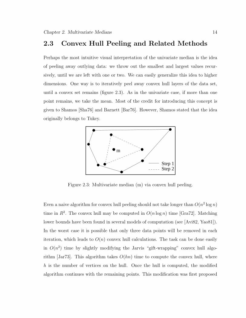
2.3 Convex Hull Peeling and Related Methods
Perhaps the most intuitive visual interpretation of the univariate median is the idea
of peeling away outlying data: we throw out the smallest and largest values recur-
sively, until we are left with one or two. We can easily generalize this idea to higher
dimensions. One way is to iteratively peel away convex hull layers of the data set,
until a convex set remains (figure 2.3). As in the univariate case, if more than one
point remains, we take the mean. Most of the credit for introducing this concept is
given to Shamos [Sha76] and Barnett [Bar76]. However, Shamos stated that the idea
originally belongs to Tukey.
Step 1Step 2
m
Figure 2.3: Multivariate median (m) via convex hull peeling.
Even a naive algorithm for convex hull peeling should not take longer than O(n2 log n)
time in R2. The convex hull may be computed in O(n log n) time [Gra72]. Matching
lower bounds have been found in several models of computation (see [Avi82, Yao81]).
In the worst case it is possible that only three data points will be removed in each
iteration, which leads to O(n) convex hull calculations. The task can be done easily
in O(n2) time by slightly modifying the Jarvis “gift-wrapping” convex hull algo-
rithm [Jar73]. This algorithm takes O(hn) time to compute the convex hull, where
h is the number of vertices on the hull. Once the hull is computed, the modified
algorithm continues with the remaining points. This modification was first proposed

Chapter 2. Multivariate Medians 15
by Shamos [Sha76]. Later Overmars and van Leeuwen [OvL81] designed a data struc-
ture which maintains the convex hull of a set of points after the insertion/deletion
of arbitrary points, with a cost of O(log2 n) time per insertion/deletion. This pro-
vides an O(n log2 n) time method for convex hull peeling. Finally, Chazelle [Cha85]
improved this result by ignoring insertions and taking advantage of the structure in
the sequence of deletions in convex hull peeling. Chazelle’s algorithm uses O(n log n)
time to compute all convex layers and the depth of any point.
A technique similar to convex hull peeling was proposed by Titterington [Tit78].
He proposed iteratively peeling minimum volume ellipsoids containing the data set.
Both methods of peeling data can have very low breakdown points. Donoho and
Gasko [DG92] proved that the breakdown point of these methods cannot exceed
1d+1
in Rd and stated that the breakdown point seems to always approach 0 as n
approaches infinity. In figure 2.4 we show how the breakdown point can approach 0
for a specific configuration of points. There is only one point inside the convex hull
so it is the median. It can be moved an arbitrary distance to the right, as long as its
nearest neighbor is moved by the same amount.
Another ellipsoid method was proposed by Rousseeuw [Rou85]. His median is the
center of the minimum volume ellipsoid that covers approximately half of the data
points. Rousseeuw proves that this estimator is invariant under affine transformations
and has a 50% breakdown point for data in general position.
Figure 2.4: Example of how the breakdown point of convex hull peeling can be made
to approach zero.

Chapter 2. Multivariate Medians 16
2.4 The Oja Simplex Median
Consider d+1 points in Rd. These points form a simplex, which has a d-dimensional
volume. For example, in R3 four points form a tetrahedron, and in R2 three points
form a triangle whose area is “2-dimensional volume”. Now consider a data set in Rd
for which we seek the median. Oja proposed the following measure for a query point
θ in Rd [Oja83] (see figure 2.5):
• for every subset of d points from the data set, form a simplex with θ.
• sum together the volumes of all such simplices.
We can call this sum Oja depth. The Oja simplex median is any point µ in Rd with
minimum Oja depth.
θθθ
θ θ θ
Figure 2.5: The simplices considered for a candidate Oja median (θ) in R2. (n = 4)
Since one-dimensional volume is length, the Oja median reduces to the standard
univariate median. In R1, the Oja median minimizes the sum of distances to all
data points, as does the L1 median. Unlike the L1 median, the Oja median is not
guaranteed to be a unique point in higher dimensions. However Oja mentions (without
proof) that the points of maximum depth form a convex set and that to compute such
a point in R2 it suffices to consider only intersection points of lines formed by pairs

Chapter 2. Multivariate Medians 17
of data points. We prove these properties in chapter 4. An important feature of the
Oja median is that it is invariant to affine transformations. However, data sets may
be constructed for which the breakdown point approaches zero. Notice that if the
data does not “span” the dimension of the space that it is in (ex: data on a line in
R2 or data on a plane in R3, then it is possible to find simplices with zero volume
even at infinity. This seems like an unrealistic case for any application though. A
nicer example for R2 is given by Niinimaa, Oja and Tableman [NOT90], although the
example used resembles a bimodal distribution and the corrupted points cannot be
moved in arbitrary directions.
The straightforward method of calculating the Oja median is to compute the depth
of each intersection point. In R2 this can be done in O(n6) time: for each of the O(n4)
intersection points there are O(n2) triangles for which the area must be computed,
and the area of a triangle can be computed in constant time. The same upper bound
holds for an algorithm of Niinimaa, Oja and Nyblom [NON92]. The algorithm selects
a line between two data points and computes the gradient of Oja depth at each
intersection point along the line until one such point is found to be a minimum. A
new line from this point is then selected, and the procedure is repeated. The gradient
is computed in O(n2) time and it is possible that all intersection points will be visited.
Rousseeuw and Ruts [RR96] provided a technique for computing the Oja gradient in
O(n log n) time and stated that the same algorithm can be used to find the median
in O(n5 log n) time. In chapter 4 we propose an algorithm which computes the Oja
median in O(n3 log n) time.
2.5 The Simplicial Median
Another interpretation of the univariate median is that it is the point which lies inside
the greatest number of intervals constructed from the data points. Liu generalized this
idea as follows [Liu90]: the simplicial median in Rd is a point in Rd which is contained
Chapter 2. Multivariate Medians 18
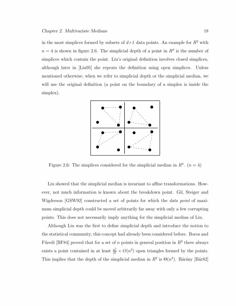
in the most simplices formed by subsets of d+1 data points. An example for R2 with
n = 4 is shown in figure 2.6. The simplicial depth of a point in Rd is the number of
simplices which contain the point. Liu’s original definition involves closed simplices,
although later in [Liu95] she repeats the definition using open simplices. Unless
mentioned otherwise, when we refer to simplicial depth or the simplicial median, we
will use the original definition (a point on the boundary of a simplex is inside the
simplex).
Figure 2.6: The simplices considered for the simplicial median in R2. (n = 4)
Liu showed that the simplicial median is invariant to affine transformations. How-
ever, not much information is known about the breakdown point. Gil, Steiger and
Wigderson [GSW92] constructed a set of points for which the data point of maxi-
mum simplicial depth could be moved arbitrarily far away with only a few corrupting
points. This does not necessarily imply anything for the simplicial median of Liu.
Although Liu was the first to define simplicial depth and introduce the notion to
the statistical community, this concept had already been considered before. Boros and
Furedi [BF84] proved that for a set of n points in general position in R2 there always
exists a point contained in at least n3
27+ O(n2) open triangles formed by the points.
This implies that the depth of the simplicial median in R2 is Θ(n3). Barany [Bar82]
Chapter 2. Multivariate Medians 19
showed that in Rd there always exists a point contained in
1
(d + 1)d+1
n
d + 1
+ O(nd)
simplices.
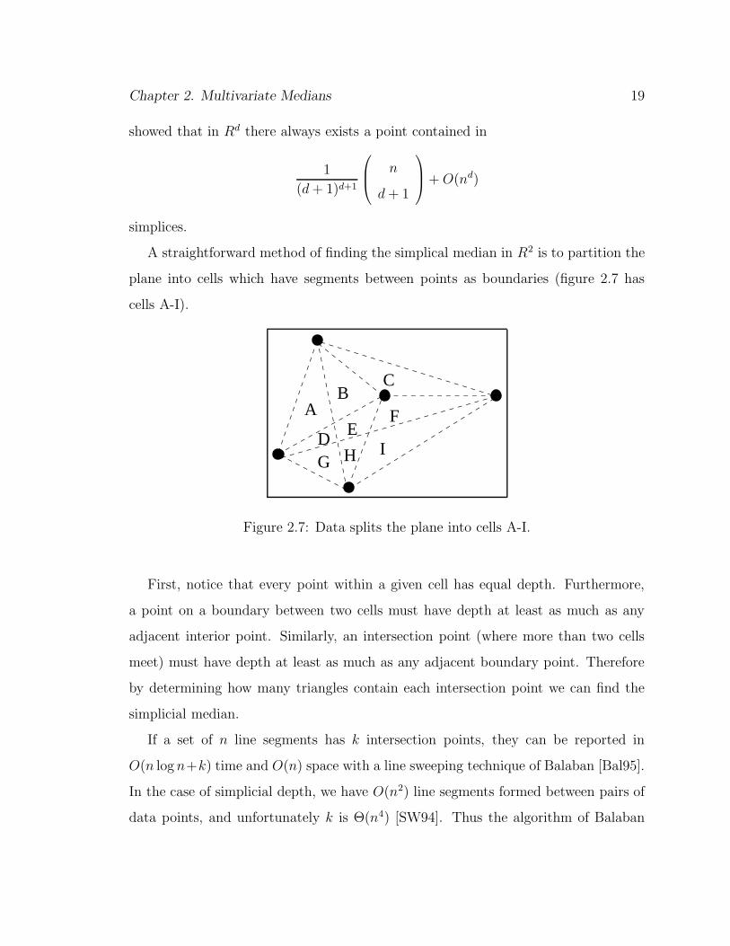
A straightforward method of finding the simplical median in R2 is to partition the
plane into cells which have segments between points as boundaries (figure 2.7 has
cells A-I).
AB
C
DE
F
G H I
Figure 2.7: Data splits the plane into cells A-I.
First, notice that every point within a given cell has equal depth. Furthermore,
a point on a boundary between two cells must have depth at least as much as any
adjacent interior point. Similarly, an intersection point (where more than two cells
meet) must have depth at least as much as any adjacent boundary point. Therefore
by determining how many triangles contain each intersection point we can find the
simplicial median.
If a set of n line segments has k intersection points, they can be reported in
O(n log n+k) time and O(n) space with a line sweeping technique of Balaban [Bal95].
In the case of simplicial depth, we have O(n2) line segments formed between pairs of
data points, and unfortunately k is Θ(n4) [SW94]. Thus the algorithm of Balaban
Chapter 2. Multivariate Medians 20
takes O(n4) time and O(n2) space for our purposes, so it is better to use brute-force to
compute each intersection point. The total time for this is O(n4) and the space used is
O(n). Since there are O(n3) triangles formed by n points, a brute-force calculation of
the simplicial median uses O(n7) time and O(n) space. Khuller and Mitchell [KM89]
proposed an O(n logn) time algorithm to compute the number of triangles formed by
triples of a data set which contain a query point in R2. Their algorithm came just
before Liu’s definition. Gil, Steiger and Wigderson [GSW92] independently proposed
the same algorithm and considered the simplicial median to be the data point with
maximum depth. A third version of this algorithm appeared later, but also inde-
pendently, by Rousseeuw and Ruts [RR96]. We describe the technique and provide
a matching lower bound for this problem in chapter 3. Rousseeuw and Ruts where
the first to point out that by computing the depth of each intersection point, the
simplicial median may be found in O(n5 log n) time. In Chapter 4 we propose algo-
rithms which further reduce this time complexity. We compute the simplicial median
in O(n4 log n) time using O(n2) space, or in O(n4) time and space.
For R3 Gil, Steiger and Wigderson [GSW92] proposed an algorithm to compute the
simplicial depth of a point in O(n2). Cheng and Ouyang [CO98] discovered a slight
flaw in this algorithm and provided a corrected version. They also provided a O(n4)
time algorithm for R4 and commented that for higher dimensions the brute-force
algorithm becomes better. They mention that an algorithm suggested by Rousseeuw
and Ruts [RR96] for higher dimensions seems to have some discrepancies.
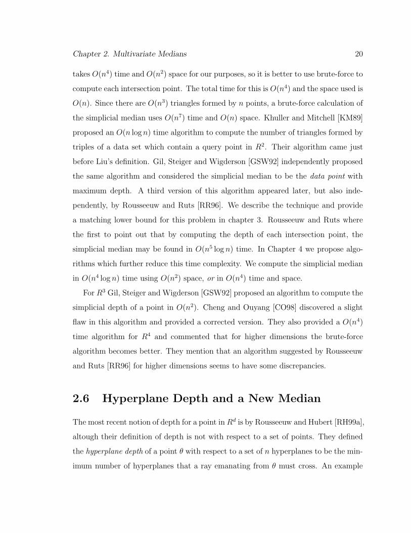
2.6 Hyperplane Depth and a New Median
The most recent notion of depth for a point in Rd is by Rousseeuw and Hubert [RH99a],
altough their definition of depth is not with respect to a set of points. They defined
the hyperplane depth of a point θ with respect to a set of n hyperplanes to be the min-
imum number of hyperplanes that a ray emanating from θ must cross. An example
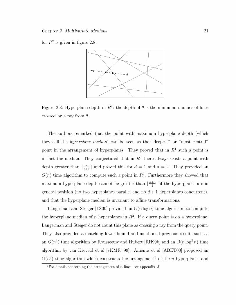
Chapter 2. Multivariate Medians 21
for R2 is given in figure 2.8.
θ
Figure 2.8: Hyperplane depth in R2: the depth of θ is the minimum number of lines
crossed by a ray from θ.
The authors remarked that the point with maximum hyperplane depth (which
they call the hyperplane median) can be seen as the “deepest” or “most central”
point in the arrangement of hyperplanes. They proved that in R1 such a point is
in fact the median. They conjectured that in Rd there always exists a point with
depth greater than d nd+1e and proved this for d = 1 and d = 2. They provided an
O(n) time algorithm to compute such a point in R2. Furthermore they showed that
maximum hyperplane depth cannot be greater than bn+d2c if the hyperplanes are in
general position (no two hyperplanes parallel and no d + 1 hyperplanes concurrent),
and that the hyperplane median is invariant to affine transformations.
Langerman and Steiger [LS00] provided an O(n log n) time algorithm to compute
the hyperplane median of n hyperplanes in R2. If a query point is on a hyperplane,
Langerman and Steiger do not count this plane as crossing a ray from the query point.
They also provided a matching lower bound and mentioned previous results such as
an O(n3) time algorithm by Rousseeuw and Hubert [RH99b] and an O(n log2 n) time
algorithm by van Kreveld et al [vKMR+99]. Amenta et al [ABET00] proposed an
O(nd) time algorithm which constructs the arrangement1 of the n hyperplanes and
1For details concerning the arrangement of n lines, see appendix A.

Chapter 2. Multivariate Medians 22
uses a breadth first search to locate the hyperplane median in Rd. They also proved
the conjecture of Rousseeuw and Hubert.
Although hyperplane depth is equivalent to the median in R1, no generalization
has been made for the multivariate median of a set of points in Rd. The concept of
a ray intersecting a minimum number of hyperplanes may be used as follows: given
a set S of n points in Rd, construct the set H of hyperplanes formed by subsets of
d points in S. Find the point µ with maximum hyperplane depth with respect to
H. The point µ can be called the H–median of S. The algorithm of Langerman
and Steiger would compute the bivariate H–median in O(n2 log n) time, since there
are O(n2) hyperplanes in R2 for a set of n points. It makes sense that for a given
point p we should consider that a ray from p does not cross hyperplanes containing p.
Otherwise, even the points on the convex hull of the data set would have significant
depth.

Chapter 3
Algorithms and Lower Bounds for
Depth in R2
In this chapter, some recent and new results concerning the depth of a query point in
R2 are presented. In section 3.1 we describe simplified versions of the algorithms
of Rousseeuw and Ruts [RR96] for computing halfspace and simplicial depth in
O(n log n) time. Their simplicial depth algorithm is practically the same as those
by Khuller and Mitchell [KM89], and by Gil, Steiger and Wigderson [GSW92]. In
section 3.2 we prove that the computation of halfspace and simplicial depth requires
Ω(n log n) time, which matches the upper bounds of these algorithms. Finally in sec-
tion 3.3 we show that our lower bounds also apply for the sign tests of Hodges [Hod55]
and of Oja and Nyblom [ON89].
3.1 Algorithms for the Depth of a Point in R2
3.1.1 Halfspace Depth Calculation
Suppose we have a data set S of n points, and a point θ for which we want to compute
halfspace depth. First, note that it suffices to consider only halfspaces determined
23
Chapter 3. Algorithms and Lower Bounds for Depth in R2 24
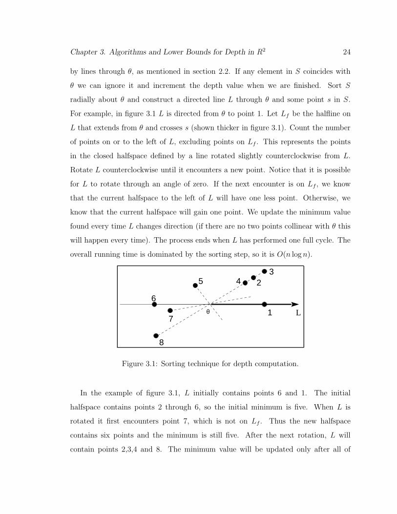
by lines through θ, as mentioned in section 2.2. If any element in S coincides with
θ we can ignore it and increment the depth value when we are finished. Sort S
radially about θ and construct a directed line L through θ and some point s in S.
For example, in figure 3.1 L is directed from θ to point 1. Let Lf be the halfline on
L that extends from θ and crosses s (shown thicker in figure 3.1). Count the number
of points on or to the left of L, excluding points on Lf . This represents the points
in the closed halfspace defined by a line rotated slightly counterclockwise from L.
Rotate L counterclockwise until it encounters a new point. Notice that it is possible
for L to rotate through an angle of zero. If the next encounter is on Lf , we know
that the current halfspace to the left of L will have one less point. Otherwise, we
know that the current halfspace will gain one point. We update the minimum value
found every time L changes direction (if there are no two points collinear with θ this
will happen every time). The process ends when L has performed one full cycle. The
overall running time is dominated by the sorting step, so it is O(n logn).
θ
23
45
6
7
8
1 L
Figure 3.1: Sorting technique for depth computation.
In the example of figure 3.1, L initially contains points 6 and 1. The initial
halfspace contains points 2 through 6, so the initial minimum is five. When L is
rotated it first encounters point 7, which is not on Lf . Thus the new halfspace
contains six points and the minimum is still five. After the next rotation, L will
contain points 2,3,4 and 8. The minimum value will be updated only after all of
Chapter 3. Algorithms and Lower Bounds for Depth in R2 25
these points are processed. The minimum will become four, corresponding to points
5 through 8. By continuing this process we find that the halfspace depth of θ is equal
to two, and is found when Lf crosses point 7.
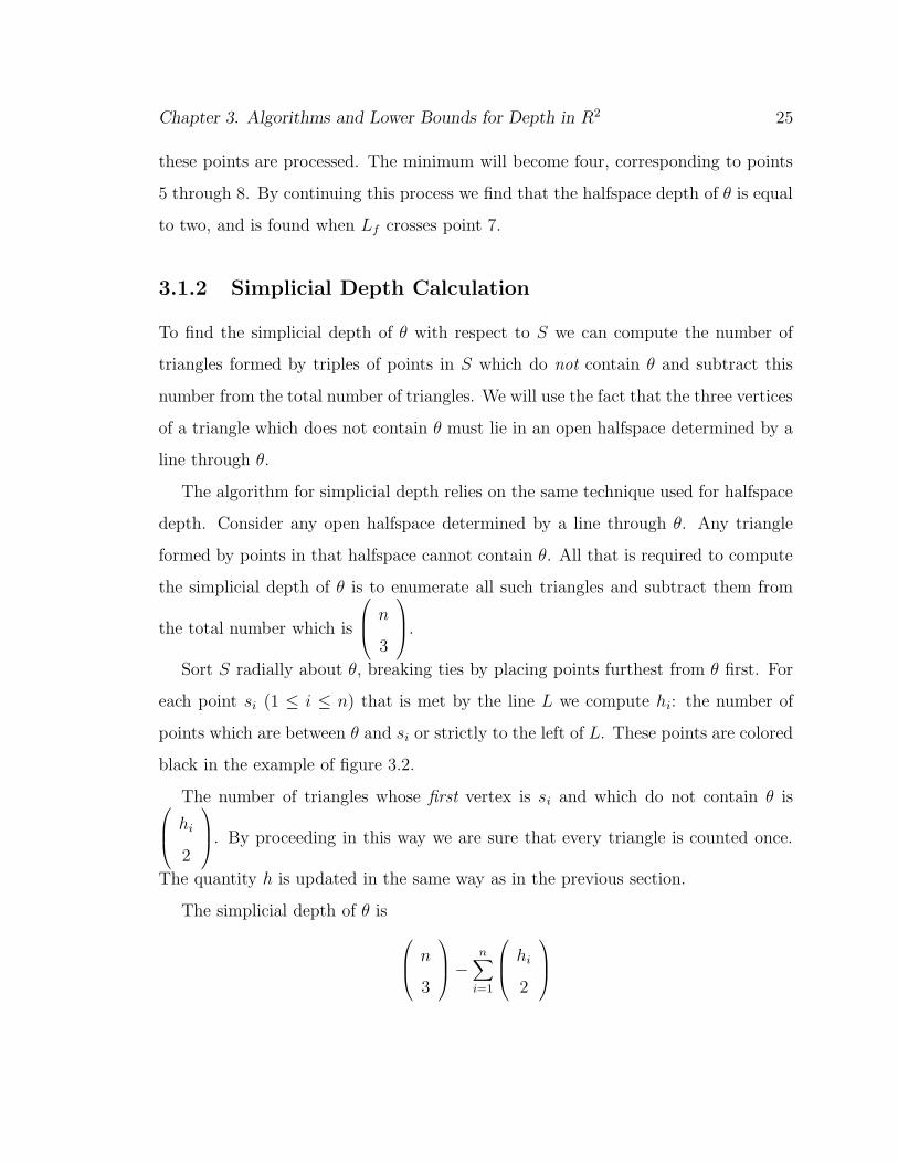
3.1.2 Simplicial Depth Calculation
To find the simplicial depth of θ with respect to S we can compute the number of
triangles formed by triples of points in S which do not contain θ and subtract this
number from the total number of triangles. We will use the fact that the three vertices
of a triangle which does not contain θ must lie in an open halfspace determined by a
line through θ.
The algorithm for simplicial depth relies on the same technique used for halfspace
depth. Consider any open halfspace determined by a line through θ. Any triangle
formed by points in that halfspace cannot contain θ. All that is required to compute
the simplicial depth of θ is to enumerate all such triangles and subtract them from
the total number which is
n
3
.
Sort S radially about θ, breaking ties by placing points furthest from θ first. For
each point si (1 ≤ i ≤ n) that is met by the line L we compute hi: the number of
points which are between θ and si or strictly to the left of L. These points are colored
black in the example of figure 3.2.
The number of triangles whose first vertex is si and which do not contain θ is
hi
2
. By proceeding in this way we are sure that every triangle is counted once.
The quantity h is updated in the same way as in the previous section.
The simplicial depth of θ is
n
3
−n
∑
i=1
hi
2

Chapter 3. Algorithms and Lower Bounds for Depth in R2 26
isθ
Figure 3.2: Simplicial depth calculation: si is the first vertex for any triangle formed
by si and two black points.
where
p
q
is zero if p < q.
The complexity is identical to that of calculating halfspace depth.
3.2 Lower Bounds for Computing the Depth of a
Point in R2
In this section we prove that computing simplicial and halfspace depths requires
Ω(n log n) time.
3.2.1 Halfspace Depth Lower Bound
We show that finding halfspace depth allows us to answer the question of Set Equality,
which has an Ω(n log n) lower bound in the algebraic decision tree model of compu-
tation [BO83]:
• Set Equality: Given two sets A = a1, a2, . . . , an and B = b1, b2, . . . , bn, is
A = B?
Chapter 3. Algorithms and Lower Bounds for Depth in R2 27
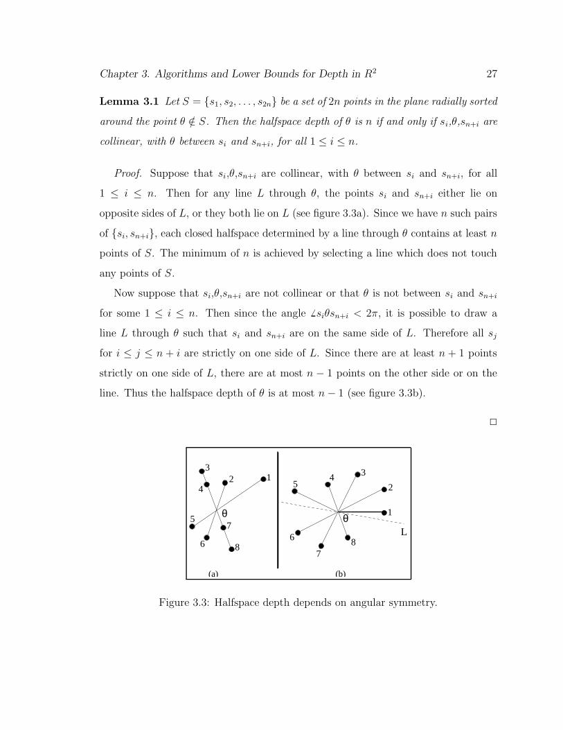
Lemma 3.1 Let S = s1, s2, . . . , s2n be a set of 2n points in the plane radially sorted
around the point θ /∈ S. Then the halfspace depth of θ is n if and only if si,θ,sn+i are
collinear, with θ between si and sn+i, for all 1 ≤ i ≤ n.
Proof. Suppose that si,θ,sn+i are collinear, with θ between si and sn+i, for all
1 ≤ i ≤ n. Then for any line L through θ, the points si and sn+i either lie on
opposite sides of L, or they both lie on L (see figure 3.3a). Since we have n such pairs
of si, sn+i, each closed halfspace determined by a line through θ contains at least n
points of S. The minimum of n is achieved by selecting a line which does not touch
any points of S.
Now suppose that si,θ,sn+i are not collinear or that θ is not between si and sn+i
for some 1 ≤ i ≤ n. Then since the angle 6 siθsn+i < 2π, it is possible to draw a
line L through θ such that si and sn+i are on the same side of L. Therefore all sj
for i ≤ j ≤ n + i are strictly on one side of L. Since there are at least n + 1 points
strictly on one side of L, there are at most n − 1 points on the other side or on the
line. Thus the halfspace depth of θ is at most n− 1 (see figure 3.3b).
2
1 24
θ
6
3
1
2
345
6
7
Lθ
8
(a) (b)
7
8
5
Figure 3.3: Halfspace depth depends on angular symmetry.
Chapter 3. Algorithms and Lower Bounds for Depth in R2 28
Theorem 3.2 Halfspace depth requires Ω(n log n) time in the worst case.
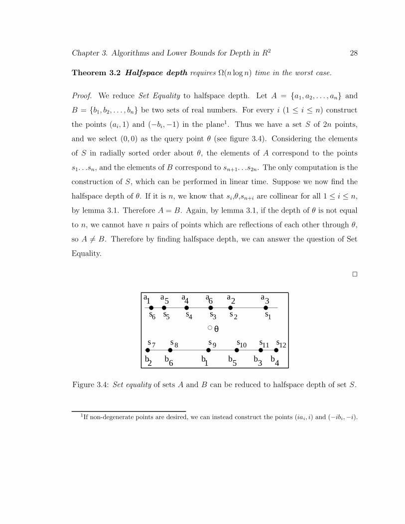
Proof. We reduce Set Equality to halfspace depth. Let A = a1, a2, . . . , an and
B = b1, b2, . . . , bn be two sets of real numbers. For every i (1 ≤ i ≤ n) construct
the points (ai, 1) and (−bi,−1) in the plane1. Thus we have a set S of 2n points,
and we select (0, 0) as the query point θ (see figure 3.4). Considering the elements
of S in radially sorted order about θ, the elements of A correspond to the points
s1. . .sn, and the elements of B correspond to sn+1. . .s2n. The only computation is the
construction of S, which can be performed in linear time. Suppose we now find the
halfspace depth of θ. If it is n, we know that si,θ,sn+i are collinear for all 1 ≤ i ≤ n,
by lemma 3.1. Therefore A = B. Again, by lemma 3.1, if the depth of θ is not equal
to n, we cannot have n pairs of points which are reflections of each other through θ,
so A 6= B. Therefore by finding halfspace depth, we can answer the question of Set
Equality.
2
θ
a a a a a a
b b b bbb
1 5 4 32
12
6
2 16 5 3 4
ssssss
s s s s s s
123456
7 8 9 10 11
Figure 3.4: Set equality of sets A and B can be reduced to halfspace depth of set S.
1If non-degenerate points are desired, we can instead construct the points (iai, i) and (−ibi,−i).

Chapter 3. Algorithms and Lower Bounds for Depth in R2 29
3.2.2 Simplicial Depth Lower Bound
We show that finding simplicial depth allows us to answer the question of Element
Uniqueness, which has an Ω(n log n) lower bound in the algebraic decision tree model
of computation [BO83]:
• Element Uniqueness: Given a set A = a1, a2, . . . , an, is there a pair i 6= j
such that ai = aj?
Theorem 3.3 Simplicial depth requires Ω(n log n) time in the worst case.
Proof. We reduce Element Uniqueness to simplicial depth. Let A = a1, a2, . . . , an
be a set of real numbers, for n ≥ 3. For every ai where 1 ≤ i ≤ n construct the points
(ai, 1) and (−ai,−1) which are reflections of each other through (0,0). Thus we have
a set S of 2n points. si and sn+i are reflections of each other through the origin,
which we select as the query point θ.
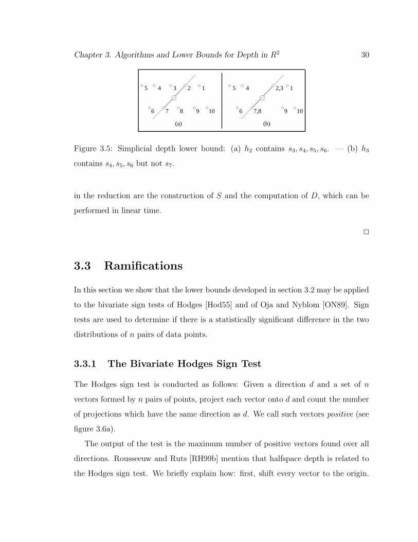
Suppose si is a unique element in S. Then the quantity hi, as defined in sec-
tion 3.1.2, must equal n − 1, since hi includes all points si+1, . . . , sn+i−1 (see fig-
ure 3.5a). Thus if no element is duplicated in S, the simplicial depth of θ with
respect to S must be
D =
2n
3
−2n∑
i=1
n− 1
2
.
Now suppose si = si+1 for some i. Then hi+1 < n− 1, since hi+1 includes at most
the points si+2, . . . , sn+i−1. It does not include the reflection of si (see figure 3.5b).
Thus if some element is duplicated in S, the simplicial depth of θ with respect to S
is strictly higher than if S has no repeated elements. Therefore by finding simplicial
depth, we can answer the question of Element Uniqueness: the elements of A are
unique if and only if the depth of (0,0) with respect to S is D. The only computations
Chapter 3. Algorithms and Lower Bounds for Depth in R2 30
6
145
9 10
2,3
7,8
(b)
6
12345
7 8 9 10
(a)
Figure 3.5: Simplicial depth lower bound: (a) h2 contains s3, s4, s5, s6. — (b) h3
contains s4, s5, s6 but not s7.
in the reduction are the construction of S and the computation of D, which can be
performed in linear time.
2
3.3 Ramifications
In this section we show that the lower bounds developed in section 3.2 may be applied
to the bivariate sign tests of Hodges [Hod55] and of Oja and Nyblom [ON89]. Sign
tests are used to determine if there is a statistically significant difference in the two
distributions of n pairs of data points.
3.3.1 The Bivariate Hodges Sign Test
The Hodges sign test is conducted as follows: Given a direction d and a set of n
vectors formed by n pairs of points, project each vector onto d and count the number
of projections which have the same direction as d. We call such vectors positive (see
figure 3.6a).
The output of the test is the maximum number of positive vectors found over all
directions. Rousseeuw and Ruts [RH99b] mention that halfspace depth is related to
the Hodges sign test. We briefly explain how: first, shift every vector to the origin.

Chapter 3. Algorithms and Lower Bounds for Depth in R2 31
1
v4
v3
v5
v2
v3
v
v
5
(a)
v4v1
d
v2
d (b)
Figure 3.6: v3 and v4 are positive vectors with respect to direction d.
This does not influence any directions, so the output of the test is unaffected. Now
notice that for a given direction d the number of positive vectors is determined by a
halfspace orthogonal to d (figure 3.6b). It is now clear that the maximum number
of positive vectors over all directions is the complement of the halfspace depth of the
origin.
Theorem 3.4 The bivariate Hodges sign test requires Ω(n log n) time in the worst
case.
Proof. The halfspace depth of a query point θ with respect to a data set of n
points may be determined by constructing n vectors (from θ to each data point) in
linear time and applying the Hodges sign test to these vectors.
2
3.3.2 The Bivariate Oja-Nyblom Sign Test
Given a data set of n points, the sign test of Oja and Nyblom involves computing
the number of triples of points, each of which has the property that it falls on the
same side of some line through the origin. Rousseeuw and Ruts [RR96] mention that
their methods, described in section 3.1, may be used to compute this sign test. The
relation to the problem of computing simplicial depth is clear.

Chapter 3. Algorithms and Lower Bounds for Depth in R2 32
Theorem 3.5 The Oja-Nyblom sign test requires Ω(n log n) time in the worst case.
Proof. The simplicial depth of a query point θ with respect to a data set of n
points may be determined by applying the Oja-Nyblom sign test to the data, taking
θ as the origin.
2

Chapter 4
New Median Algorithms
In this chapter we present new algorithms for computing two bivariate medians. In
section 4.1 we present our algorithms for the Oja median. Algorithm Oja–1 has a
time complexity of O(n3 log n) and uses O(n2) space. Our gradient descent algorithm,
Oja–2, uses O(n4) time and O(n2) space. It may be also be used to find the Fermat-
Torricelli points of n lines in O(n2) time and O(n) space. In section 4.2 we present
our algorithm for computing the simplicial median, which uses O(n4 log n) time and
O(n2) space or O(n4) time and space. As mentioned in chapter 2, our algorithms
for computing the Oja and simplicial medians improve the time complexity of the
algorithms by Rousseeuw and Ruts which use O(n5 log n) time. Our algorithm for
computing the Fermat-Torricelli points of n lines improves the one by Barbara which
uses O(n3) time.
4.1 Oja Median Algorithms
4.1.1 Properties of the Oja Median in R2
Some properties of the Oja median in R2 are first stated and proved. Let L be the
set of lines formed by each pair of points in a data set S. Note that by “Oja median”
33

Chapter 4. New Median Algorithms 34
we mean one point for which Oja depth is minimum. If other such points exist it is
an easy matter to find them, as should be apparent after the proof of lemma 4.4.
Lemma 4.1 The Oja depth of a point θ with respect to S can be expressed as a
weighted sum of the distances from θ to each line in L.
Proof. By definition, Oja depth is the sum of the areas of all triangles (θ,si, sj), where
1 ≤ i < j ≤ n. The area of each triangle may be expressed as 12bh, where b is the
distance from si to sj and h is the orthogonal distance from the point θ to the line
sisj.
2
Lemma 4.2 The Oja median must be on one of the intersection points of the lines
in L.
Proof. Each cell formed by the arrangement of lines in L can be considered to be
a linear program1 , where the feasible region is determined by the edges of the cell,
and the function to be minimized is the weighted sum of lemma 4.1. Therefore if the
median is located within a given cell, it must be on one of its vertices. The median
cannot be at infinity (as part of an open cell) since the Oja depth would be infinite,
as is apparent by lemma 4.1.
2
Lemma 4.3 The Oja depth along any line ` in the plane varies in a piecewise-linear
manner, with inflection points occurring only where ` crosses lines in L.
Proof. The rate of change of Oja depth is constant along ` within any cell of the
arrangement of lines, since the cell represents a linear program. As ` crosses from one
1For an introduction to linear programming, see [Chv83].

Chapter 4. New Median Algorithms 35
cell to the next, it crosses from one linear program to another. The transition occurs
at the common edge of two cells, which is on a line in L.
2
Lemma 4.4 The Oja depth along a line ` has only one local minimum, from which
the rate of change of Oja depth increases monotonically in both directions.
Proof. Suppose that the Oja depth is decreasing as we move along ` in some direction,
and that along this direction we encounter line m which is a member of L. This
encounter does not affect the contribution of any other line in L to Oja depth. Since
crossing m can only increase m’s contribution to Oja depth, the result is that Oja
depth cannot decrease at a faster rate. Since Oja depth decreases from infinity as
we approach the members of L from either direction on `, the lemma follows by
induction. The local minimum can be a point or a segment between two intersection
points.
2
In figure 4.1 we illustrate lemma 4.4. If Oja depth f(`) is decreasing along ` as we
approach m, the situation of figure 4.1 cannot exist.
f(l)
l
m
Figure 4.1: Oja depth f(`) cannot decrease at a faster rate when crossing m.

Chapter 4. New Median Algorithms 36
Corollary 4.5 The Oja depth function is convex.
Proof. A bivariate function f is convex if, for every x1, x2 ∈ R2 and every α,
0 ≤ α ≤ 1, there holds
f(αx1 + (1− α)x2) ≤ αf(x1) + (1− α)f(x2).
By lemma 4.4, the above property holds for Oja depth.
2
Corollary 4.6 The points in R2 with minimum Oja depth form a convex polygon
with O(n) vertices on its boundary.
Proof. Since the Oja depth function is a convex polyhedron, the minimum value must
be at a vertex, a line segment or a face of the polyhedron, all of which are convex.
If we project these objects back onto the plane, we obtain an intersection point, a
boundary segment on a cell, or a single cell in the arrangement of L. Every data point
can contribute at most two lines to the boundary of a cell, so every cell has O(n)
segments on its boundary. Thus the number of intersection points with minimum Oja
depth is O(n).
2
Lemma 4.7 If the Oja depth decreases along two directions u and v from a point p,
then it must also decrease in all directions between u and v (within the acute angle).
Proof. All points along u or v from p have depth less than the depth at p. Between
any point along u and any point along v we can form a line, along which the depth
cannot have a local maximum, by lemma 4.4. Therefore the depth along this line
and between the two points cannot be greater than the depth of both points, which
implies that the depth cannot be greater than the depth at p. This also implies that
Chapter 4. New Median Algorithms 37
from any point p, the directions in which depth increases must span at least 180o.
Otherwise Oja depth would decrease in all directions from p, which contradicts the
fact that there can be no local maximum.
2
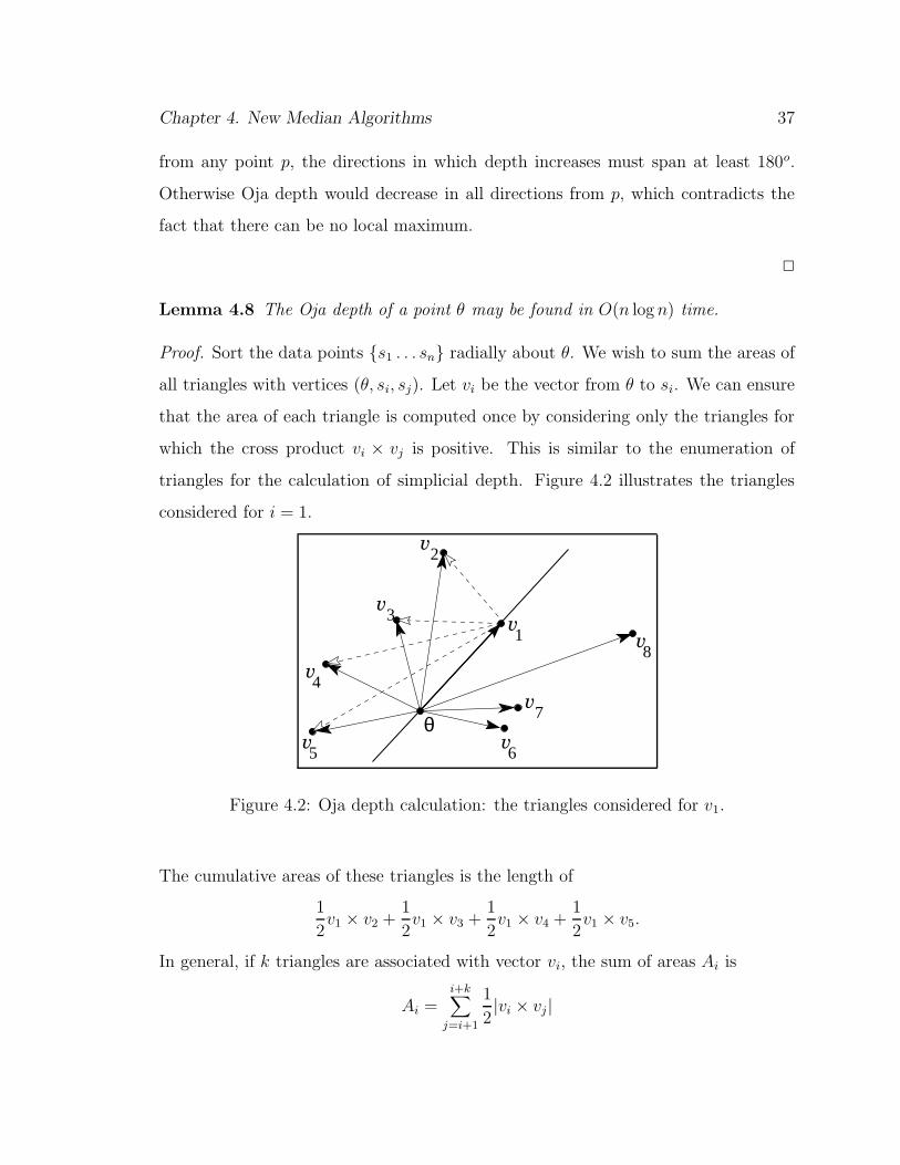
Lemma 4.8 The Oja depth of a point θ may be found in O(n log n) time.
Proof. Sort the data points s1 . . . sn radially about θ. We wish to sum the areas of
all triangles with vertices (θ, si, sj). Let vi be the vector from θ to si. We can ensure
that the area of each triangle is computed once by considering only the triangles for
which the cross product vi × vj is positive. This is similar to the enumeration of
triangles for the calculation of simplicial depth. Figure 4.2 illustrates the triangles
considered for i = 1.
θ
v1 v
8
v
v6
v
v
v4
v5
7
2
3
Figure 4.2: Oja depth calculation: the triangles considered for v1.
The cumulative areas of these triangles is the length of
1
2v1 × v2 +
1
2v1 × v3 +
1
2v1 × v4 +
1
2v1 × v5.
In general, if k triangles are associated with vector vi, the sum of areas Ai is
Ai =i+k∑
j=i+1
1
2|vi × vj|
Chapter 4. New Median Algorithms 38
where j is taken modulo n. Using a basic cross-product relation we get
Ai =1
2vi × (vi+1 + vi+2 + · · ·+ vi+k). (4.1)
A1 may be computed in O(n) time. Now we proceed through the sorted list of vectors,
as in the halfspace depth calculation. Every time we encounter a vector, we add it or
subtract it from the vector sum in equation 4.1, in the same way that we updated the
contents of each halfspace. Since each vector will be added and subtracted once, this
process takes O(n) time to compute all remaining Ai. Therefore the time complexity
of this procedure is dominated by the initial sorting step.
2
We can use figure 4.2 to give an example of the above procedure. Initially we have
A1 = 12v1 × V , where V is the vector sum of v2,v3,v4,v5. When we sweep a line
through the vectors in a counterclockwise direction, we first encounter v2. Thus we
subtract v2 from V and compute A2 = 12v2 × V . When we reach v4, V will be equal
to v5. After v4 the rotating line will cross v6 and v7, which are added to V . Therefore
A5 = 12v5 × (v6 + v7).
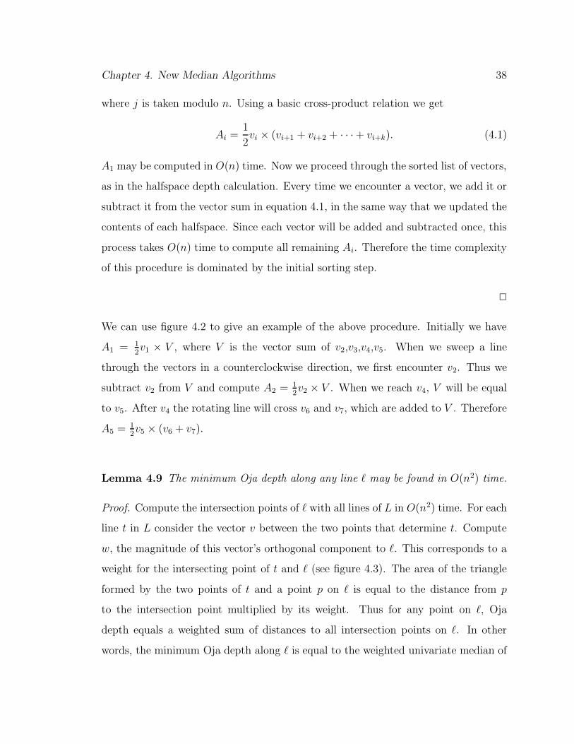
Lemma 4.9 The minimum Oja depth along any line ` may be found in O(n2) time.
Proof. Compute the intersection points of ` with all lines of L in O(n2) time. For each
line t in L consider the vector v between the two points that determine t. Compute
w, the magnitude of this vector’s orthogonal component to `. This corresponds to a
weight for the intersecting point of t and ` (see figure 4.3). The area of the triangle
formed by the two points of t and a point p on ` is equal to the distance from p
to the intersection point multiplied by its weight. Thus for any point on `, Oja
depth equals a weighted sum of distances to all intersection points on `. In other
words, the minimum Oja depth along ` is equal to the weighted univariate median of
Chapter 4. New Median Algorithms 39
O(n2) points. This may be computed in O(n2) time with a slight modification of the
univariate median algorithm of Blum et al [BFP+73] mentioned in the introduction
(chapter 1).
2
pl
t
v
w
Figure 4.3: Calculating Oja depth on a line.
Note that as with the univariate median, the minimum Oja depth along a line
may be computed by first sorting all the intersection points. This would increase the
complexity by a factor of log n.
4.1.2 The two Algorithms
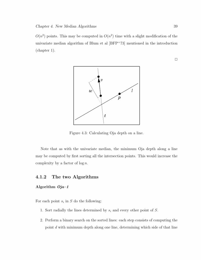
Algorithm Oja–1
For each point si in S do the following:
1. Sort radially the lines determined by si and every other point of S.
2. Perform a binary search on the sorted lines: each step consists of computing the
point d with minimum depth along one line, determining which side of that line

Chapter 4. New Median Algorithms 40
contains directions where the depth does not increase from d, and proceeding
in that region of space.
3. If a line is found where depth only increases from d, halt and return d.
In figure 4.4, suppose we have sorted all lines from si to other data points. We
start the binary search with lines a and b which split the plane into four quadrants
containing roughly the same number of lines. Now after computing the minimum Oja
depth on a and b, we restrict the location of the Oja median to one quadrant. If it
is the upper-left quadrant, we continue the binary search by selecting line c, which
again splits the remaining list of lines evenly.
is
c
b
a
Figure 4.4: Algorithm Oja–1: For each data point si perform a binary search on the
lines to other data points.
Theorem 4.10 Algorithm Oja–1 computes the bivariate Oja median of n points in
O(n3 log n) time and O(n2) space.
Proof. Binary search is made possible by lemma 4.7, which implies that for a point
with minimum depth along a line, the depth must increase in all directions of at least
one side of the line. The region in which to proceed may be found by using the gradi-
ent of the Oja depth function, which can be computed in O(n2) time by Niinimaa, Oja
and Nyblom [NON92] or in O(n log n) time by Rousseeuw and Ruts [RR96]. Thus the

Chapter 4. New Median Algorithms 41
complexity of one step in the binary search is dominated by calculating the minimum
depth on a line, which takes O(n2) time by lemma 4.9. The binary search continu-
ously shrinks a wedge in the plane where the Oja median may be found, or in other
words expands the region where the median cannot be found. Since by lemma 4.2
the median must be located on one of the lines in L, there must exist a data point
for which this wedge will shrink to a single line. The minimum depth along this
line is the Oja median. O(n2) ∗ O(log n) time suffices for one data point. Thus the
total complexity for step 2 is O(n3 log n). This dominates the time complexity of this
algorithm since step 1 takes O(n2 log n) time by brute force or O(n2) with a method
described in Appendix A. The amount of space used is O(n2) for step 1.
2
Algorithm Oja–2
Choose any line in L and label it as `.
1. Find the point p with minimum Oja depth on `.
2. Find the intersecting line at p which has the steepest rate of change of Oja
depth (this is done in a similar way to finding which region to proceed in during
algorithm Oja–1). If the steepest slope is not negative then stop. Otherwise,
label the line with steepest slope as ` and go to step 1.
Theorem 4.11 Algorithm Oja–2 computes the bivariate Oja median of n points in
O(n4) time and O(n2) space.
Proof. Due to lemma 4.7 we know that once the region on one side of a line is rejected,
the line will never be re-visited by a gradient descent. Since the function is convex,
the descent must succeed after visiting O(n2) lines. By lemma 4.9, O(n2) time suffices
Chapter 4. New Median Algorithms 42
for step 1. Thus the total complexity amounts to O(n4). Only one line is processed
at a time, so the space used is O(n2).
2
Note that we could also simply find the minimum depth on each of the O(n2) lines
without using a gradient descent. The complexity would only differ by a constant
factor.
4.1.3 The Fermat-Torricelli Points of n Lines
In section 4.1.1, lemmas 4.1 and 4.2 imply that the Oja median is a Fermat-Torricelli
point of L. However we cannot use algorithm Oja–1 for any set of lines, since this
algorithm relies on the fact that a large number of lines pass through each point in
S. Instead algorithm Oja–2 may be used since it assumes nothing about the position
of the lines. Therefore we have the following theorem:
Theorem 4.12 The Fermat-Torricelli points of n lines may be computed in O(n2)
time and O(n) space, using algorithm Oja–2.
4.2 Simplicial Median Algorithm
Let S be a data set of n points in R2, and I be the set of line segments formed between
every pair of points in S.
Lemma 4.13 To find a point with maximum simplicial depth it suffices to consider
the intersection points of segments in I.
Proof. Consider the arrangement of cells whose boundaries are segments in I. All
points in the interior of a given cell must have equal simplicial depth. Any point on
the boundary of this cell must have depth at least equal to points in the interior.

Chapter 4. New Median Algorithms 43
Finally, any vertex of the cell must have depth at least equal to any point on an
adjacent boundary. These vertices are the intersection points of segments in I.
2
To simplify the description of our algorithm for computing the simplicial median,
assume that S is in general position, in the sense that no three points are collinear.
Later we explain how this assumption may be removed, if desired, without influencing
the time or space complexity.
Algorithm Simp-Med
1. Calculate the simplicial depth of every data point in S.
2. Compute the number of points which are strictly to one side of each segment
in I (each side separately).
3. For every segment ` in I,
(a) compute and sort the intersection points of all other segments with `, if
there are any.
(b) let MAX be the greatest depth among the endpoints of `.
(c) if there exist other intersection points on `, calculate the simplicial depth
d of the intersection point adjacent to one of the endpoints. Update MAX
(if MAX < d, MAX← d).
(d) continue through the sorted list: every time an intersecting line is left
behind, subtract from d the number of points strictly behind the line.
Every time a line is encountered, add to d the number of points strictly
ahead of that line. Update MAX after encountering each intersection.
4. Exit with the greatest MAX value found over all segments, and the associated
intersection point.

Chapter 4. New Median Algorithms 44
Figure 4.5 illustrates the logic behind step 3 of algorithm Simp-Med. Once we know
the depth of an intersection point (step 3c), we can compute all other depths along
the given segment, each in constant time. Each intersecting segment forms a triangle
with every point strictly to one side. Thus every time we encounter a segment, we
enter as many triangles as there are points on the other side of this segment. Every
time we leave a segment behind, we exit triangles formed by that segment and each
point on the other side. So in figure 4.5, suppose we are moving from left to right
along the current line segment, and just before encountering segment t, we have some
value d = 10. Upon encountering t, we can see that we are now inside three new
triangles: one for each point to the right of t. As soon as we move to the right of
t, we will no longer be inside five triangles. So on t, d = 13, and immediately after,
d = 8.
CURRENT
t
Figure 4.5: Algorithm Simp–Med: the current line segment traversed, and an inter-
secting segment t.
In case we have multiple segments intersecting the current line at the same point,
we may form a temporary list of these segments. When the last one is encountered,
we process the list: First we add the points to the right of each line, then we subtract
all the points to the left of each line.
Chapter 4. New Median Algorithms 45
Theorem 4.14 Algorithm Simp-Med computes the bivariate simplicial median of n
points in O(n4 log n) time and O(n2) space or alternatively in O(n4) time and space.
Proof. All intersection points are checked, so by lemma 4.13 a point of maximum
simplicial depth is found. Step 1 takes O(n2 log n) time in total since the calculation
of simplicial depth for a point takes O(n logn) time with the algorithm of Rousseeuw
and Ruts [RR96]. Step 2 is straightforward to do in O(n3) time by brute force.
Step 3a takes O(n2 log n), 3b is constant, 3c is O(n log n), and 3d takes O(n2) time.
Thus step 3 takes O(n4 log n) once run for every segment, and dominates the time
complexity of this algorithm. The space used is O(n2) for steps 2 and 3a. If we
compute the arrangement2 of I in O(n4) time and space as preprocessing, then step
3a is no longer necessary. In this case, the preprocessing step would dominate the
complexity of the algorithm.
2
We note that certain steps of algorithm Simp–Med may be performed more effi-
ciently, without improving the asymptotic complexity overall (apart from some con-
stant factor). For example take step 2 where we count the number of points on each
side of every line segment. The problem of counting or reporting the points to one
side of a query line has been the focus of extensive research in the past. Of course,
this problem is of interest only when several queries are made. Typically some form
of preprocessing takes place which allows each query to be answered in less than the
brute-force O(n) time. Chazelle, Guibas and Lee [CGL85] compute the convex lay-
ers of the given data set as a preprocessing step (in O(n log n) time using Chazelle’s
algorithm mentioned in chapter 2). Then they report every point on one side of a
query line in O(k + log n) time, where k is the number of points reported. Since we
only need to count the points in step 2, we describe only the relevant portions of their
2This concept is described in Appendix A.

Chapter 4. New Median Algorithms 46
algorithm. A given query line is tested for intersection with every convex layer. This
may be done in O(log vi) time for layer i which has vi vertices, by performing a binary
search on the edges of the layer. If the line and convex layer intersect, it is an easy
matter to count the number of points on each side of the query line in constant time.
This is done by considering the indices of the layer’s segments which intersect the
query line. We see that the time complexity T (n) depends on the number of convex
layers k:
T (n) =k
∑
i=1
O(log vi)
where∑k
i=1 vi = n. If there is one layer, T (n) becomes O(log n), but if there are
O(n) layers, T (n) is O(n). The expected number of convex hull layers for a uniform
distribution of data points in a convex area is Ω(n2
3 ) and O(n2
3 log1
3 n) [Dev01]. In
the case that the lower bound is achieved, T (n) is O(n2
3 log n). The algorithm of
Edelsbrunner and Welzl [EW86] uses O(n logn) preprocessing time and then takes
O(k+n0.695) time for each query. However, in this algorithm if points are only counted
the time complexity reduces to O(n0.695). The total space used is O(n). Agarwal
and Erickson [AE98] provide an extensive survey on this problem and similar topics,
including a discussion of lower bounds and time-space tradeoffs. Since step 2 of
algorithm Simp–Med performs O(n2) queries, the algorithm of Chazelle, Guibas and
Lee takes O(n3) time in the worst case, but will have a better time complexity than
the brute-force method for some data distributions. The algorithm of Edelsbrunner
and Welzl takes O(n2.695) time for step 2. By taking advantage of the structure of
the lines in this problem, we can further reduce this time complexity. This is done by
using a procedure similar to that mentioned in section 3.1.1. For every data point, we
essentially compute halfspace depth, but store the points counted for every halfplane
considered. Therefore step 2 can be performed in O(n2 log n) time. Furthermore, it
is possible to sort all points about each point in O(n2) time (see [LC85, Ede87] or
Appendix A) , so the halfspace depth procedure then takes only O(n) time per data
Chapter 4. New Median Algorithms 47
point. This means that the time complexity of step 2 reduces to O(n2). The same
applies for computing the simplicial depth of all data points in step 1.
Finally we explain how the general position assumption may be removed. Steps 1
and 2 are not affected. While performing step 3a for some line `, if we encounter an
intersection point which happens to be a data point, we can simply stop processing `
and go to the next segment. We may do this because the intersecting data point will
form segments with both endpoints of `, so all points on ` will be processed anyway.
This leaves one more case to consider. Suppose that if we extend an intersecting
segment t we will find c collinear points. We can determine this easily since we know
the number of points strictly to the side of t. It follows that we must also have
more intersecting segments collinear with t. If there are m such segments, then we
claim that on this intersection point we are inside m(c−2)2
triangles, apart from those
considered by the regular algorithm. We arrive at this number from the following
argument: With the endpoints of an intersecting segment and one of the other c
points, we can form a triangle containing the intersection point. Therefore using the
two endpoints we can form c− 2 such triangles. Suppose that x is the third point for
one of these triangles. Then x and one of the endpoints will form another intersecting
segment. So the same triangle will be counted exactly one more time when the other
segment is processed. Therefore we have c − 2 triangles counted for each of the m
segments, and we multiply by a factor of 12
to avoid counting each triangle twice.

Chapter 5
Conclusion
We have presented an overview of several estimators of location, including an account
of recent developments on robustness and computational complexity issues. Emphasis
was given to estimators which have a geometrical aspect to them. The most important
elements of this thesis were the new results obtained concerning bivariate depths and
estimators of location.
We have defined a new median for n points in any dimension, by adapting the
hyperplane depth of Rousseeuw and Hubert to a set of points. Properties of this
median may be studied easily through simulations in the near future, since relatively
fast algorithms for hyperplane depth already exist.
We have proved that the computation of simplicial or halfspace depth for one point
in R2 requires Ω(n log n) time. Thus we have matched the upper bound complexity
of the algorithms of Rousseeuw and Ruts. In addition, we have shown that the
computation of the bivariate sign tests of Hodges and of Oja and Nyblom require
Ω(n log n) time. Recently we learned that a different lower bound proof for halfspace
depth was obtained independently by Langerman and Steiger [LS00].
We have reduced the complexity of calculating the Oja and simplicial medians. The
Oja median may be computed in O(n3 log n) time and O(n2) space. The simplicial
48

Chapter 5. Conclusion 49
median may be computed in O(n4 log n) time with O(n2) space, or alternatively, in
O(n4) time and space. This improves the results of Rousseeuw and Ruts, whose
algorithms compute each median in O(n5 log n) time. Our algorithm Oja–2 may be
used to compute the Fermat-Torricelli points of n lines in O(n2) time and O(n) space,
thus improving the algorithm of Barbara which takes O(n3) time. Furthermore, our
proof that the solution must be on an intersection point is much shorter.
This research has left certain open problems, which we list below:
Conjecture 5.1 The computation of Oja depth requires Ω(n log n) time.
Open Problem 5.2 Prove conjecture 5.1, or disprove it by providing a procedure
faster than that described in lemma 4.8.
Open Problem 5.3 What are the highest attainable lower bounds for computing the
halfspace, simplicial, Oja and H–medians in R2?
As mentioned in section 2.6 the algorithm of Langerman and Steiger may be
used to compute the bivariate H–median of n points in O(n2 log n) time. However,
their algorithm was designed to work for arbitrarily placed hyperplanes, whereas the
hyperplanes considered for the H–median have some structure.
Open Problem 5.4 Can the O(n2 log n) time algorithm for computing the H–median
be improved?
Open Problem 5.5 What are the breakdown points of the simplicial and H–medians?
Since the submission of this thesis, some of the results obtained have been im-
proved [ALST01]. The Oja median may be computed in O(n log3 n) time and O(n)
space, and the Fermat–Torricelli points of n lines may be computed in O(n) time and
space. We are optimistic that in the near future we will also be able to improve our
algorithm for the simplicial median, and we intend to study the alternate definition
involving open simplices.

Appendix A
Arrangements of Lines
Consider a set L of n lines in the plane. As we can see in figure A.1, L splits the plane
into convex cells, line segments and intersection points. This partition of the plane is
known as an arrangement of lines. In computational geometry it is often convenient
to use the structure of arrangements as opposed to dealing with each line separately.
Examples of applications are given in [O’R95]. We say that we have constructed the
arrangement of L if:
• for every line ` in L we have a sorted list of all intersection points on `.
• for every intersection point we have a radially sorted list of all lines intersecting
the point.
An arrangement of n lines may be constructed in Θ(n2) time and space. This
result was first obtained by Chazelle, Guibas and Lee [CGL85], and by Edelsbrunner,
O’Rourke and Seidel [EOS86]. The proof of this result is described well in [O’R95].
The same algorithm may be used to construct an arrangement of line segments.
A nice application of arrangements is for sorting all points about every point in
a data set in O(n2) time [LC85, Ede87]. This may be used in algorithms Oja–1 and
Simp–Med. We first briefly explain the concept of duality. Every point (a, b) in the
50
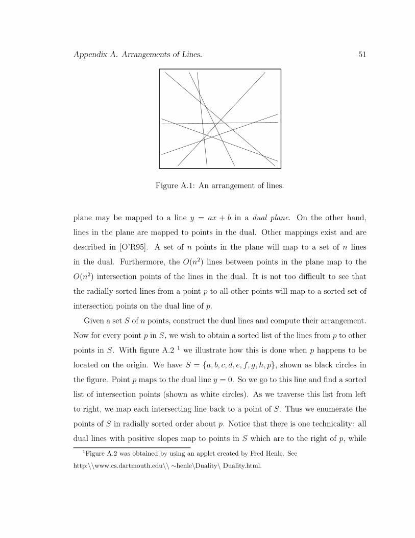
Appendix A. Arrangements of Lines. 51
Figure A.1: An arrangement of lines.
plane may be mapped to a line y = ax + b in a dual plane. On the other hand,
lines in the plane are mapped to points in the dual. Other mappings exist and are
described in [O’R95]. A set of n points in the plane will map to a set of n lines
in the dual. Furthermore, the O(n2) lines between points in the plane map to the
O(n2) intersection points of the lines in the dual. It is not too difficult to see that
the radially sorted lines from a point p to all other points will map to a sorted set of
intersection points on the dual line of p.
Given a set S of n points, construct the dual lines and compute their arrangement.
Now for every point p in S, we wish to obtain a sorted list of the lines from p to other
points in S. With figure A.2 1 we illustrate how this is done when p happens to be
located on the origin. We have S = a, b, c, d, e, f, g, h, p, shown as black circles in
the figure. Point p maps to the dual line y = 0. So we go to this line and find a sorted
list of intersection points (shown as white circles). As we traverse this list from left
to right, we map each intersecting line back to a point of S. Thus we enumerate the
points of S in radially sorted order about p. Notice that there is one technicality: all
dual lines with positive slopes map to points in S which are to the right of p, while
1Figure A.2 was obtained by using an applet created by Fred Henle. See
http:\\www.cs.dartmouth.edu\\ ∼henle\Duality\ Duality.html.

Appendix A. Arrangements of Lines. 52
dual lines with negative slopes map to points to the left of p. However we wish to
manage this, it may be done in O(n) time. Therefore this process takes O(n2) time
for all points in S.
a
b
c
d
d
ef
g
a
h
b c ef g hp
X
Y
Figure A.2: A set of points and their dual lines.
Bibliography
[ABET00] N. Amenta, M. Bern, D. Eppstein, and S. Teng. Regression depth and
center points. Discrete and Computational Geometry, 123(3):305–323,
2000.
[ACG+01] G. Aloupis, C. Cortes, F. Gomez, M. Soss, and G. Toussaint. Lower
bounds for computing statistical depth. Technical Report SOCS-01.1,
School of Computer Science, McGill University, February 2001.
[AE98] P. Agarwal and J. Erickson. Geometric range searching and its relatives.
In J. Goodman B. Chazelle and R. Pollack, editors, Advances in Discrete
and Computational Geometry. AMS Press, Providence, RI, 1998.
[ALST01] G. Aloupis, S. Langerman, M. Soss, and G. Toussaint. Algorithms for
bivariate medians and a Fermat-Torricelli problem for lines. Submitted
for publication, 2001.
[AST01] G. Aloupis, M. Soss, and G. Toussaint. On the computation of the
bivariate median and a Fermat-Torricelli problem. Technical Report
SOCS-01.2, School of Computer Science, McGill University, February
2001.
[Avi82] D. Avis. On the complexity of finding the convex hull of a set of points.
Discrete Applied Math, 4:81–86, 1982.
53

Bibliography 54
[Bal95] I. Balaban. An optimal algorithm for finding segment intersections. In
Proc. 11th Annu. ACM Sympos. Comput. Geom., pages 211–219, 1995.
[Bar76] V. Barnett. The ordering of multivariate data. Journal of the Royal
Statistical Society ser.A, 139:318–355, 1976.
[Bar82] I. Barany. A generalization of Caratheodory’s theorem. Discrete Math,
40:141–150, 1982.
[Bar00] R. Barbara. The Fermat-Torricelli points of n lines. Mathematical
Gazette, 84:24–29, 2000.
[Bas91] G. Bassett. Equivariant monotonic, 50% breakdown estimators. The
American Statistician, 45(2):135–137, 1991.
[BF84] E. Boros and Z. Furedi. The maximal number of covers by the triangles
of a given vertex set on the plane. Geom. Dedicata, 17:69–77, 1984.
[BFP+73] M. Blum, R. Floyd, V. Pratt, R. Rivest, and R. Tarjan. Time bounds
for selection. Journal of Computer and System Sciences, 7(4):448–461,
1973.
[BO83] M. Ben-Or. Lower bounds for algebraic computation trees. In Proc. 15th
Ann. ACM Sympos. Theory Comput., pages 80–86, 1983.
[CGL85] B. Chazelle, L. Guibas, and D. Lee. The power of geometric duality.
BIT, 25:76–90, 1985.
[Cha85] B. Chazelle. On the convex layers of a planar set. IEEE Transactions
on Information Theory, IT-31(4):509–517, 1985.
[Chv83] V. Chvatal. Linear Programming. W. H. Freeman, New York, NY, 1983.

Bibliography 55
[CLR90] T. Cormen, C. Leierson, and R. Rivest. Introduction to Algorithms. MIT
Press, 1990.
[CO98] A. Cheng and M. Ouyang. On algorithms for simplicial depth. Technical
Report dcs-tr-368, Department of Computer Science, Rutgers University,
1998.
[CSY87] R. Cole, M. Sharir, and K. Yap. On k-hulls and related problems. SIAM
J. Comput., 16(1):61–77, 1987.
[Dev01] L. Devroye. The expected number of peels of a random cloud of points.
manuscript, 2001.
[dF34] P. de Fermat. Abhandlungen uber maxima und minima. Ostwalds Klas-
siker der exacten Wissenschaften, M. Miller (ed), 238, 1934.
[DG92] D. Donoho and M. Gasko. Breakdown properties of location estimates
based on halfspace depth and projected outlyingness. Annals of Statis-
tics, 20:1803–1827, 1992.
[DH83] D. Donoho and P. Huber. The notion of breakdown point. In P. Bickel,
K. Doksum, and J. Hodges, editors, A Festschrift for Erich L. Lehmann,
pages 157–184, Belmont, California, 1983. Wadsworth International
Group.
[Don82] D. Donoho. Breakdown properties of multivariate location estimators.
Ph.D. thesis, Harvard University, 1982.
[Ede87] H. Edelsbrunner. Algorithms in Combinatorial Geometry. Springer-
Verlag, Berlin, 1987.
[Eel30] W. Eells. A mistaken conception of the center of population. Journal of
the American Statistical Association, 25:33–40, 1930.

Bibliography 56
[EOS86] H. Edelsbrunner, J. O’Rourke, and R. Seidel. Constructing arrangements
of lines and hyperplanes with applications. SIAM J. Comput., 15(2):341–
363, 1986.
[EW86] H. Edelsbrunner and E. Welzl. Halfplanar range search in linear space
and O(n0.695) query time. Inform. Process. Lett., 23:289–293, 1986.
[Gal33] L. Galvani. Sulla determinazione del centro di gravita e del centro me-
diano di una popolazione. Metron, 11(1):17–47, 1933.
[GG29] C. Gini and L. Galvani. Di talune estensioni dei concetti di media a
caratteri qualitivi. Metron, 8:3–209, 1929.
[Gow74] J. Gower. The mediancentre. Applied Statistics, 23(3):466–470, 1974.
[Gra72] R. Graham. An efficient algorithm for determining the convex hull of a
finite planar set. Information Processing Letters, 7:175–180, 1972.
[Gre81] P. J. Green. Peeling bivariate data. In V. Barnett, editor, Interpreting
Multivariate Data, New York, 1981. Wiley.
[Gri27] F. Griffin. Abstract: Points of minimum travel for a distributed popu-
lation. Bulletin of the American Mathematical Society, 33:516, 1927.
[GS98] C. Groß and T. Strempel. On generalizations of conics and on a gen-
eralization of the Fermat-Torricelli problem. American Mathematical
Monthly, 105(8):732–743, 1998.
[GSW92] J. Gill, W. Steiger, and A. Wigderson. Geometric medians. Discrete
Mathematics, 108:37–51, 1992.
[Ham68] R. Hampel. Contributions to the theory of robust estimation. Ph.D.
thesis, University of California, Berkeley, 1968.
Bibliography 57
[Har69] F. Harary. Graph Theory. Addison-Wesley, Reading, Mass., 1969.
[Hay02] J. Hayford. What is the center of an area, or the center of a population?
Journal of the American Statistical Association, 8:47–58, 1902.
[Hod55] J. Hodges. A bivariate sign test. In Annals of Mathematical Statistics,
volume 26, pages 523–527, 1955.
[Hod67] J. Hodges. Efficiency in normal samples and tolerance of extreme values
for some estimates of location. In 5th Berkeley Symposium on Mathe-
matical Statistics and Probability, volume 1, pages 163–186, 1967.
[Hot29] H. Hotelling. Stability in competition. Economic Journal, 39:41–57,
1929.
[Hub72] P. Huber. Robust statistics: A review. The Annals of Mathematical
Statistics, 43(3):1041–1067, 1972.
[Jar73] R. Jarvis. On the identification of the convex hull of a finite set of points
in the plane. Information Processing Letters, 2:18–21, 1973.
[JM94] S. Jadhav and A. Mukhopadhyay. Computing a centerpoint of a finite
planar set of points in linear time. Discrete and Computational Geome-
try, 12:291–312, 1994.
[KM89] S. Khuller and J. Mitchell. On a triangle counting problem. Information
Processing Letters, 33:319–321, 1989.
[Knu76] D. Knuth. Big omicron and big omega and big theta. ACM SIGACT
News, 2:18–43, 1976.
[Lan01] S. Langerman. Algorithms and Data Structures in Computational Geom-
etry. Ph.D. thesis, Department of Computer Science, Rutgers University,
New Brunswick, 2001.

Bibliography 58
[LC85] D. Lee and Y. Ching. The power of geometric duality revisited. Infor-
mation Processing Letters, 21:117–122, 1985.
[Liu90] R. Liu. On a notion of data depth based upon random simplices. The
Annals of Statistics, 18:405–414, 1990.
[Liu95] R. Liu. Control charts for multivariate processes. Journal of the Amer-
ican Statistical Association, 90(432):1380–1387, 1995.
[Lop92] H. Lopuhaa. Highly efficient estimator of multivariate location. The
Annals of Statistics, 20(1):398–413, 1992.
[LPS99] R. Liu, J. Parelius, and K. Singh. Multivariate analysis of data depth:
descriptive statistics and inference. Annals of Statistics, 27(3):783–858,
1999.
[LS00] S. Langerman and W. Steiger. The complexity of hyperplane depth in the
plane. In Japan Conference on Discrete and Computational Geometry,
November 2000.
[LV19] G. Loria and G. Vassura, editors. Opere di Evangelista Torricelli, vol-
ume 1. Faenza, 1919.
[Mat91] J. Matousek. Computing the center of planar point sets. In J. Good-
man, R. Pollack, and W. Steiger, editors, Computational Geometry: Pa-
pers from the DIMACS special year, volume 6, pages 221–230. American
Mathematical Society, 1991.
[Moo41] A. Mood. On the joint distribution of the medians in samples from a
multivariate population. The Annals of Mathematical Statistics, 12:268–
278, 1941.

Bibliography 59
[MRR+01] K. Miller, S. Ramaswami, P. Rousseeuw, T. Sellares, D. Souvaine,
I. Streinu, and A. Struyf. Fast implementation of depth contours us-
ing topological sweep. In Proc. 12th Symposium on Discrete Algorithms
(SODA), Washington D.C., 2001.
[NON92] A. Niinimaa, H. Oja, and J. Nyblom. Algorithm AS 277: The Oja
bivariate median. Applied Statistics, 41:611–617, 1992.
[NOT90] A. Niinimaa, H. Oja, and M. Tableman. The finite-sample breakdown
point of the Oja bivariate median and of the corresponding half-samples
version. Statistics and Probability Letters, 10:325–328, 1990.
[Oja83] H. Oja. Descriptive statistics for multivariate distributions. Statistics
and Probability Letters, 1:327–332, 1983.
[ON89] H. Oja and J. Nyblom. Bivariate sign tests. Journal of the American
Statistical Association, 84(405):249–259, 1989.
[O’R95] J. O’Rourke. Computational Geometry in C. Cambridge University
Press, 1995.
[OvL81] M. Overmars and J. van Leeuwen. Maintenance of configurations in the
plane. J. Comput. and Syst. Sci., 23:166–204, 1981.
[PS80] W. Paul and J. Simon. Decision trees and random access machines. Logic
and Algorithmics, Monograph 30, L’Enseignement Mathematique, 1980.
[PS85] F. Preparata and M. Shamos. Computational Geometry. An Introduc-
tion. Springer-Verlag, 1985.
[RH99a] P. Rousseeuw and M. Hubert. Depth in an arrangement of hyperplanes.
Discrete Computational Geometry, 22:167–176, 1999.

Bibliography 60
[RH99b] P. Rousseeuw and M. Hubert. Regression depth. Journal of the American
Statistical Association, 94:388–402, 1999.
[RL91] P. Rousseeuw and H. Lopuhaa. Breakdown points of affine equivariant
estimators of multivariate location and covariance matrices. The Annals
of Statistics, 119(1):229–248, 1991.
[Ros30] F. Ross. Editor’s note on the center of population and point of mini-
mum travel. Journal of the American Statistical Association, 25:447–452,
1930.
[Rou85] P. Rousseeuw. Multivariate estimation with high breakdown point. In
W. Grossman, G. Pflug, I. Vincze, and W. Wertz, editors, Mathematical
Statistics and Applications, volume B, pages 283–297, Dordrecht, 1985.
Reidel Publishing Company.
[RR96] P. Rousseeuw and I. Ruts. Bivariate location depth. Applied Statistics,
45:516–526, 1996.
[RR98] P. Rousseeuw and I. Ruts. Constructing the bivariate Tukey median.
Statistica Sinica, 8:828–839, 1998.
[RR99] P. Rousseeuw and I. Ruts. The depth function of a population distribu-
tion. Metrika, 49(3):213–244, 1999.
[Sca33] D. Scates. Locating the median of the population in the United States.
Metron, 11(1):49–65, 1933.
[Sha76] M. Shamos. Geometry and statistics: Problems at the interface. In
J. Traub, editor, Recent Results and New Directions in Algorithms and
Complexity, pages 251–280. Academic Press, 1976.

Bibliography 61
[Sma90] C. Small. A survey of multidimensional medians. International Statistical
Review, 58:263–277, 1990.
[Sta81] W. Stahel. Robust Estimation: Infinitesimal optimality and covariance
matrix estimators. Ph.D. thesis, ETH, Zurich, 1981.
[SW94] E. Scheinerman and H. Wilf. The rectilinear crossing number of a com-
plete graph and Sylvester’s “four point problem” of geometric probabil-
ity. American Mathematical Monthly, 101(10):939–943, 1994.
[Tit78] D. Titterington. Estimation of correlation coefficients by ellipsoidal trim-
ming. Applied Statistics, 27:227–234, 1978.
[TP79] G. T. Toussaint and R. S. Poulsen. Some new algorithms and software
implementation methods for pattern recognition research. In Proc. IEEE
Computer Society Conf. on Computer Software, pages 55–63, 1979.
[Tuk75] J. Tukey. Mathematics and the picturing of data. In Proceedings of the
International Congress of Mathematicians, pages 523–531, Vancouver,
1975.
[vKMR+99] M. van Kreveld, J. Mitchell, P. Rousseeuw, M. Sharir, J. Snoeyink, and
B. Speckmann. Efficient algorithms for maximum regression depth. In
Proceedings of the 15th Symposium on Computational Geometry, ACM,
pages 31–40, 1999.
[Web09] A. Weber. Uber den Standort der Industrien, Tubingen. English trans-
lation by C. Friedrich (1929), Alfred Weber’s Theory of Location of In-
dustries. University of Chicago Press, 1909.
[Yao81] A. Yao. A lower bound to finding convex hulls. Journal of the ACM,
28(4):780–787, 1981.