Multidimensional modal analysis of nonlinear sloshing in a rectangular ...tim/PAPERS/JFM2000.pdf ·...
34
J. Fluid Mech. (2000), vol. 407, pp. 201–234. Printed in the United Kingdom c 2000 Cambridge University Press 201 Multidimensional modal analysis of nonlinear sloshing in a rectangular tank with finite water depth By ODD M. FALTINSEN 1 , OLAV F. ROGNEBAKKE 1 , IVAN A. LUKOVSKY 2 AND ALEXANDER N. TIMOKHA 2 1 Department of Marine Hydrodynamics, Faculty of Marine Technology, NTNU, Trondheim, N-7491, Norway 2 Institute of Mathematics, National Academy of Sciences of Ukraine, Tereschenkivska, 3 str., Kiev, 252601, Ukraine (Received 29 January 1999 and in revised form 18 October 1999) The discrete infinite-dimensional modal system describing nonlinear sloshing of an incompressible fluid with irrotational flow partially occupying a tank performing an arbitrary three-dimensional motion is derived in general form. The tank has vertical walls near the free surface and overturning waves are excluded. The derivation is based on the Bateman–Luke variational principle. The free surface motion and velocity potential are expanded in generalized Fourier series. The derived infinite-dimensional modal system couples generalized time-dependent coordinates of free surface elevation and the velocity potential. The procedure is not restricted by any order of smallness. The general multidimensional structure of the equations is approximated to analyse sloshing in a rectangular tank with finite water depth. The amplitude–frequency response is consistent with the fifth-order steady-state solutions by Waterhouse (1994). The theory is validated by new experimental results. It is shown that transients and associated nonlinear beating are important. An initial variation of excitation periods is more important than initial conditions. The theory is invalid when either the water depth is small or water impacts heavily on the tank ceiling. Alternative expressions for hydrodynamic loads are presented. The procedure facilitates simulations of a coupled vehicle–fluid system. 1. Introduction A main objective is to describe violent fluid motions (sloshing) in a partly filled tank forced to oscillate in a frequency domain close to its lowest natural frequency. The ratio between maximum free surface amplitude and characteristic tank motion amplitude is then high and significant nonlinearities occur. This has practical interest for sloshing in ship tanks. By considering sea states that a ship has to operate in, it is realistic that wave-induced ship motions can cause resonant fluid oscillations. This can lead to large local structural loads in the tank and has an important effect on the global ship motions. It is desirable to develop numerical methods that accurately describe the fluid loading and coupling between ship motions and sloshing. A necessary requirement is that long time simulations can be performed and the proper statistical distribution of response variables obtained for various sea states.
Transcript of Multidimensional modal analysis of nonlinear sloshing in a rectangular ...tim/PAPERS/JFM2000.pdf ·...
J. Fluid Mech. (2000), vol. 407, pp. 201–234. Printed in the United Kingdom
c© 2000 Cambridge University Press
201
Multidimensional modal analysis of nonlinearsloshing in a rectangular tank
with finite water depth
By O D D M. F A L T I N S E N1, O L A V F. R O G N E B A K K E1,I V A N A. L U K O V S K Y2 AND A L E X A N D E R N. T I M O K H A2
1Department of Marine Hydrodynamics, Faculty of Marine Technology, NTNU, Trondheim,N-7491, Norway
2Institute of Mathematics, National Academy of Sciences of Ukraine, Tereschenkivska, 3 str.,Kiev, 252601, Ukraine
(Received 29 January 1999 and in revised form 18 October 1999)
The discrete infinite-dimensional modal system describing nonlinear sloshing of anincompressible fluid with irrotational flow partially occupying a tank performing anarbitrary three-dimensional motion is derived in general form. The tank has verticalwalls near the free surface and overturning waves are excluded. The derivation is basedon the Bateman–Luke variational principle. The free surface motion and velocitypotential are expanded in generalized Fourier series. The derived infinite-dimensionalmodal system couples generalized time-dependent coordinates of free surface elevationand the velocity potential. The procedure is not restricted by any order of smallness.The general multidimensional structure of the equations is approximated to analysesloshing in a rectangular tank with finite water depth. The amplitude–frequencyresponse is consistent with the fifth-order steady-state solutions by Waterhouse (1994).The theory is validated by new experimental results. It is shown that transients andassociated nonlinear beating are important. An initial variation of excitation periodsis more important than initial conditions. The theory is invalid when either the waterdepth is small or water impacts heavily on the tank ceiling. Alternative expressions forhydrodynamic loads are presented. The procedure facilitates simulations of a coupledvehicle–fluid system.
1. IntroductionA main objective is to describe violent fluid motions (sloshing) in a partly filled
tank forced to oscillate in a frequency domain close to its lowest natural frequency.The ratio between maximum free surface amplitude and characteristic tank motionamplitude is then high and significant nonlinearities occur. This has practical interestfor sloshing in ship tanks. By considering sea states that a ship has to operate in,it is realistic that wave-induced ship motions can cause resonant fluid oscillations.This can lead to large local structural loads in the tank and has an importanteffect on the global ship motions. It is desirable to develop numerical methodsthat accurately describe the fluid loading and coupling between ship motions andsloshing. A necessary requirement is that long time simulations can be performedand the proper statistical distribution of response variables obtained for various seastates.
202 O. M. Faltinsen, O. F. Rognebakke, I. A. Lukovsky and A. N. Timokha
Several studies on different numerical approaches to sloshing have been reportedby Su Tsung-Chow (1992), Buechmann (1996), Tanizawa (1996), Chen et al. (1997),Pawell (1997) and the Loads Committee of the 13th ISSC (Moan & Berge 1997). Ageneral drawback is the limited ability to perform long time simulations, especiallyfor coupled ‘liquid–structure’ interactions. It may also be difficult to find water impactloads and local structural response. One reason is that water impact studies wouldoften require a very fine discretization in time and space. Hydroelasticity may alsohave to be considered. We have instead focused on developing a semi-analyticalmethod based on modal modelling. The present method assumes a smooth tank.This implies that potential theory can be used. The method also requires verticaltank walls near the mean free surface in its equilibrium position. Overturning wavescannot be described. It will be shown that a high degree of analysis can be performed.The consequences are both a time efficient and robust method. Water impact is notstudied in detail, but the method can be combined with a local slamming analysis(see Faltinsen & Rognebakke 1999) and applied to coupled ‘fluid–tank’ simulations.An example is given illustrating the damping effect of forceful water impact on fluidmotion.
Modal modelling of nonlinear sloshing implies that the equation of the free surfaceΣ(t): z = f(x, y, t) is expanded in generalized Fourier series by a set of natural modes.The free surface elevation and the unknown velocity potential ϕ are expressed as
z = f(x, y, t) =∑
βi(t)(surfacemode)i(x, y),
ϕ(x, y, z, t) =∑
Ri(t)(domainmode)i(x, y, z).
(1.1)
The (x, y, z) coordinate system is fixed relative to the tank; x, y are coordinates in theplane of the unperturbed water surface and t is the time variable. Generally speaking,the surface and volume modes are arbitrary known functions. However, they aretypically chosen by the relation
(surfacemode)i(x, y) = (domainmode)i(x, y, z)|Σ0, (1.2)
where Σ0 is the unperturbed free surface. Since f(x, y, t) is single-valued, (1.1) does notdescribe overturning waves. Moreover, (surfacemode)i(x, y) must have a non-varyingdomain of definition. This means the tank must have vertical walls near the freesurface in its equilibrium position.
The generalized coordinates βi and Ri are found by a coupled system of nonlinearordinary differential equations (modal system). The derivation of the modal systemfrom the original free boundary problem was first proposed by Narimanov (1957)based on a perturbation technique. It has been further developed by Dodge, Kana &Abramson (1965), Narimanov, Dokuchaev & Lukovsky (1977) and Lukovsky (1990).These and other authors used a perturbation technique combined with variational(Hamilton–Ostrogradsky) projective method and derived small-dimensional models(1–3 degrees of freedom in a vertical circular cylinder) in the generalized coordinatesβi(t) or their averaged values (for resonantly excited waves). (See for instance Lukovsky1976; Miles (1976, 1984a, b).) Using an averaging technique means that βi is written as
βi =
∞∑j=0
(〈βi〉1j (τ) sin (jσt) + 〈βi〉2j (τ) cos (jσt)),
where σ is the excitation frequency and τ is slowly varying relative to t. The averagedequations of a 〈βi〉j(τ) have the form of a Duffing equation for a rectangular tank
Multidimensional modal analysis of nonlinear sloshing 203
(see Shemer 1990 and Tsai, Yue & Yip 1990) or a system of four first-order ordinarydifferential equations for a vertical circular cylindrical tank (see Miles (1984a, b)).Funakoshi & Inoue (1991) used Miles’ model in their detailed simulations. Theaveraging technique and small-dimensional modal modelling complement eachanother in the analysis of the steady-state free surface response due to periodic tankexcitations. But these methods are questionable in modelling coupled fluid–structureinteraction with complicated non-periodic tank motions when transient effects matter.These complex motions are simulated in engineering applications either numericallyor by phenomenological (usually pendulum) models (see Chapter 5 of Narimanov etal. 1977 or Pilipchuk & Ibrahim 1997). An alternative is to use Narimanov’s originaltechnique with the modal representation in the form (1.1) and more general asymp-totic assumptions of βi and Rn in order to reach reasonable dimensions of the modalsystems. The successful use of this approach is reported by Limarchenko & Yasinsky(1997) and Lukovsky & Timokha (1995) for simplified models of spacecraft. A similarmethod was used by Ikeda & Nakagawa (1997) for analysis of damping of vesselmotions due to sloshing. This suggests that multidimensional modal analysis cansimulate complicated nonlinear wave phenomena coupled with structural vibrations.
The general form of a discrete infinite-dimensional modal system is derived in thefirst part of this paper by the Bateman–Luke (pressure-integral Lagrangian) varia-tional principle. This idea was proposed independently by Miles (1976) and Lukovsky(1976). They studied forced small-amplitude translatory motions of a vertical circularcylindrical tank. The surfacemodes and domainmodes were obtained by linear theoryand related by (1.2). Our derivation of a discrete infinite-dimensional modal systemis not restricted to a particular type of body motion. The surface and domain modesare not associated with natural modes and no asymptotic assumptions are introducedin the first stage of the derivation. The infinite-dimensional modal system can bereduced to a finite-dimensional form by assuming small-amplitude forced oscillationsand associate order of magnitudes of the different modes. This is done in the secondpart of the paper to analyse nonlinear sloshing in a two-dimensional rectangularsmooth tank with finite water depth. Both forced translatory and rotational bodymotions are considered. The lowest natural mode is assumed to dominate and thethree lowest modes interact nonlinearly with each other. Several modes having higherorder are considered by linear theory. The asymptotic theory constructed is a specialmultidimensional analogue of the model by Ikeda & Nakagawa (1997) and the directgeneralization of the third-order hydrodynamic theory by Faltinsen (1974).
Experiments on nonlinear sloshing caused by primary mode resonant excitationhave been conducted. The asymptotic modal theory constructed explains the basicobserved phenomena including modulated (‘beating’) waves with a high accuracyof amplitude and ‘beating period’ characteristics. The beating is a consequence oftransients that do not die out on a very long time scale. The reason is the verysmall damping of the fluid motion inside a smooth tank with no internal structuresobstructing the flow and no heavy water impact on the tank ceiling. A consequence isthat steady-state response of the fluid motion can have a limited capability to describesloshing quantitatively. However the steady-state response is valuable to understandimportant features of the flow like stability and how the response is influenced bywater depth, excitation frequency and amplitude. Since it represents a special caseof our theory, steady-state solutions are used in the verification process. Examplesof steady-state amplitude–frequency response for surge- and pitch-excited nonlinearwaves are presented. The results are consistent with the third- and fifth-order steady-state solutions by Faltinsen (1974) and Waterhouse (1994) respectively.
204 O. M. Faltinsen, O. F. Rognebakke, I. A. Lukovsky and A. N. Timokha
The use of a discrete modal system allows us to calculate various kinematic anddynamic characteristics occurring due to interaction between the fluid and the tank.We present examples of hydrodynamic force and moment on the tank. The structureof the equations describing the fluid motion as a function of the rigid body motionsmakes it possible to set up an equation system for the coupled tank and fluid motion.An example could be analysis of a ship tank due to wave-induced ship motions.Since the wave conditions that cause violent sloshing may not be extreme, we can uselinear time domain theory to describe external hydrodynamic loads acting on the ship.By setting up the equations of motions for the global rigid ship motions togetherwith the equations describing sloshing, complex fluid–structure interaction can beanalysed. But the theory does not describe the effect of impact on the tank ceiling.This can easily occur in practical applications and is an area of further research.The asymptotic theory is not applicable to shallow water. This is due to secondaryparametric resonance and means that the primary mode is not dominating. The ratiobetween water depth and breadth of the tank is 0.173 in the example where the finitewater depth theory does not work. This is not really shallow water in a hydrodynamiccontext (see the nonlinear theory by Verhagen & Wijngaarden 1965). What we needis a theory that can combine the present finite water depth theory with a nonlinearshallow water theory.
2. Free boundary value problemA mobile rigid tank partly filled by an inviscid incompressible fluid is considered.
The flow is irrotational. The fluid volume bounded by the free surface Σ(t) andthe wetted tank surface S(t) is denoted Q(t). Let O′x′y′z′ be an absolute coordinatesystem and Oxyz be a moving coordinate system fixed with respect to the rigid tank.The origin of Oxyz is in the unperturbed free surface and moves with the velocityv0 relative to O′x′y′z′. The tank has an angular velocity ω relative to O′x′y′z′. Thegravity field has the potential
U(x, y, z, t) = −g · r′, r′ = r′0 + r, (2.1)
where r′ is the radius-vector of a point of the body–fluid system with respect to O′,r′0 is the radius-vector of the point O with respect to O′, r is the radius-vector withrespect to O and g is the gravity acceleration vector.
Since the flow is irrotational, the fluid velocity can be represented as va = ∇Φ,where va is the fluid velocity vector at the point (x, y, z) in the moving coordinatesystem and Φ(x, y, z, t) is the velocity potential. The velocity potential and the freesurface Σ(t) can be found from the following nonlinear free boundary problem:
∆Φ = 0 in Q(t),∂Φ
∂ν= v0 · ν + ω · [r × ν] on S(t),
∂Φ
∂ν= v0 · ν + ω · [r × ν] +
ξt
|∇ξ| on Σ(t),
∂Φ
∂t+ 1
2(∇Φ)2 − ∇Φ · (v0 + ω × r) +U = 0 on Σ(t),
∫Q(t)
dQ = const.
(2.2)
Here ν is the outer normal to the boundary of Q(t) and ξ(x, y, z, t) = 0 is the equationof the free surface Σ(t). The last integral condition in (2.2) implies fluid volumeconservation and is also the well-known solvability condition for the Neumannboundary value problem.
Multidimensional modal analysis of nonlinear sloshing 205
The free boundary problem (2.2) must be completed by initial or periodicityconditions to get a unique solution. The first type of condition introduces the initialposition of the free surface Σ(t0) and the initial distribution of normal derivatives ofΦ, i.e.
ξ(t0, x, y, z) = ξ0(x, y, z),∂Φ
∂ν
∣∣∣Σ(t0)
= φ(x, y, z). (2.3)
Here ξ0(x, y, z) and φ(x, y, z) are given functions. If the flow starts from rest withsufficiently small tank oscillations, linear theory can be used to formulate the initialconditions. One way of doing this is in terms of impulse conservation. This means
Φ = 0 on Σ0 and zero free surface elevation for t = t0. (2.4)
The last free surface boundary condition (dynamic boundary condition) of (2.2) isobtained by using Lagrange–Cauchy integral for the pressure in the moving coordinatesystem. It states that the pressure on the free surface is equal to a constant p0. Thehydrodynamic pressure p in Q(t) can be obtained by
∂Φ
∂t+ 1
2(∇Φ)2 − ∇Φ · (v0 + ω × r) +U +
p− p0
ρ= 0 in Q(t). (2.5)
Here ∂Φ/∂t is calculated in the moving coordinate system, i.e. for a point rigidlyconnected with the system Oxyz.
There is a set of mechanical characteristics (expressed by integrals of Φ and itsderivatives), which describes the interaction between the vessel and fluid. They are:
(a) the radius-vectors of the mass centre with respect to the points O′ and O (r′1Cand r1C) r′1C = r′0 + r1C , where
ρ
∫Q(t)
U dQ = −ρ∫Q(t)
g · r′ dQ = −m1g · r′1C;
(b) the resulting hydrodynamic forces F (t), and moments N (t) on the tank
F (t) =
∫S(t)
(p− p0)ν dS, N (t) =
∫S(t)
r × ((p− p0)ν) dS. (2.6)
3. Derivation of the general modal system by the variational methodLet us consider the boundary value problem (2.2). The unknowns are Φ =
Φ(x, y, z, t) and ξ(x, y, z, t). We will use a Bateman–Luke variational principle andintroduce the pressure in the Lagrangian of the Hamilton principle. The idea of thepressure integral as the Lagrangian in hydrodynamic problems was first proposed byHargneaves (1908). The canonical formulation of this principle is given by Bateman(1944) and Luke (1967) (for gravity surface waves in infinite basins). We use theformulation given by Lukovsky (1990).Pressure-integral Lagrangian variational principle. The boundary value
problem given by (2.2) can be described by examining the necessary conditions forthe extrema of the functional
W =
∫ t2
t1
L dt, (3.1)
206 O. M. Faltinsen, O. F. Rognebakke, I. A. Lukovsky and A. N. Timokha
where the Lagrangian L is the pressure integral
L =
∫Q(t)
(p− p0) dQ = −ρ∫Q(t)
[∂Φ
∂t+ 1
2(∇Φ)2 − ∇Φ · (v0 + ω × r) +U
]dQ; (3.2)
and the test functions satisfy
δΦ(x, y, z, t1) = 0, δΦ(x, y, z, t2) = 0; δξ(x, y, z, t1) = 0, δξ(x, y, z, t2) = 0. (3.3)
We consider a domain Q having vertical walls in a neighbourhood of the freesurface in the equilibrium position. The normal velocity component on the free surface
z = f(x, y, t) is given in the body-fixed system by −ξt/|∇ξ| = ft/√
1 + f2x + f2
y . The
velocity potential is expressed as
Φ(x, y, z, t) = v0 · r + ω ·Ω+ ϕ. (3.4)
The vector-function Ω(x, y, z) = (Ω1, Ω2, Ω3) (Stokes–Zhukovsky potentials) is thesolution of the following Neumann boundary value problem:
∆Ω = 0 in Q(t),
∂Ω1
∂ν
∣∣∣S(t)+Σ(t)
= yν3 − zν2,∂Ω2
∂ν
∣∣∣S(t)+Σ(t)
= zν1 − xν3,
∂Ω3
∂ν
∣∣∣S(t)+Σ(t)
= xν2 − yν1,
(3.5)
where ν1, ν2, ν3 are the projections of the outer normal ν onto the Oxyz-axes. Thefunction ϕ is a solution of the Neumann boundary value problem
∆ϕ = 0 in Q(t),∂ϕ
∂ν
∣∣∣S(t)
= 0,∂ϕ
∂ν
∣∣∣Σ(t)
=ft√
1 + f2x + f2
y
.
The Neumann boundary value problems for Ω and ϕ have unique solutions since∫S(t)+Σ(t)
∂Ωi
∂νdS = 0,
∫Σ(t)
∂ϕ
∂νdS =
∫Σ(t)
ft√1 + (∇f)2
dS = 0
are always fulfilled (see Lukovsky & Timokha 1995). These solutions depend para-metrically on time. By using (3.4) and the boundary value problems for Ω and ϕ itfollows that Φ satisfies the Laplace equation and the Neumann boundary conditionsof (2.2). The dynamic condition (pressure balance) on Σ(t) gives the final equationconnecting f,Ω and ϕ.
Let the function f(x, y, t) be expressed as
f(x, y, t) =
∞∑i=1
βi(t)fi(x, y), (3.6)
where fi(x, y) is a complete (to within a constant) orthogonal system of functionssatisfying the condition of volume conservation
∫Σ0fi(x, y) dx dy = 0. Further,
ϕ(x, y, z, t) =
∞∑n=1
Rn(t)ϕn(x, y, z), (3.7)
where the complete system of functions ϕn(x, y, z) satisfies the Laplace equation in
Multidimensional modal analysis of nonlinear sloshing 207
the whole tank domain Q and zero Neumann boundary condition on the wettedbody surface. Normally, only the wetted body surface below the mean free surface isconsidered. Since the system ϕn(x, y, z) is complete on any single-connected surfacein the tank domain, it is also a complete system on Σ0. The Stokes–Zhukovskypotentials Ωi are assumed to be known functions of βi. Hence, we must only find theunknown functions βi(t) and Rn(t).
Such a family of harmonic functions ϕn(x, y, z) can be chosen as a set of solutionsof the following boundary spectral problems with spectral parameter λn:
∆ϕn = 0 in Q0,∂ϕn
∂ν= 0 on S,
∂ϕn
∂ν= λnϕn on Σ0,
∫Σ0
ϕn dS = 0. (3.8)
This is the same as the linear eigenvalue problem for sloshing. The solutions can befound analytically only for a limited class of tank shapes. Examples are a verticalcircular cylinder or a rectangular three-dimensional tank. However, a numericalmethod can be used to find ϕn for a general tank shape. This was demonstrated bySolaas & Faltinsen (1997), where Moiseev’s theory was applied to two-dimensionalsloshing. A different approach is to use a patching procedure and consider for instancea tank consisting of a cylindrical part near the free surface. Then the solution in thecylindrical part can be expressed as
ϕn(x, y, z) =∑k
(bnk exp (−λkz) + ank exp (λkz))φk(x, y) (3.9)
with unknown coefficients bnk and ank . Here λk and φk are the solutions of thefollowing spectral problem:
∆2φk(x, y) + λ2kφk = 0 in Σ0,
∂φk
∂n= 0 on ∂Σ0,
∫Σ0
φk dS = 0, (3.10)
where ∂Σ0 is the intersection line between Σ0 and S . The solution in the non-cylindrical part can be found by a numerical method. When the auxiliary problem(3.10) is formulated in circular (ring-shaped) or rectangular cross-sections Σ0, thesolutions φk of (3.10) are expressed by Bessel functions and/or sinusoidal functions.Otherwise, a numerical procedure for (3.10) is required.
By substituting (3.4) into (3.2) the Lagrangian L takes the following form:
L = −ρ∫Q(t)
[v0 · r +
∂
∂t(ω ·Ω) + 1
2∇(ω ·Ω) · ∇(ω ·Ω)− ω · (r × ∇(ω ·Ω))
− 12v2
0 − ω · (r × v0)− ω · (r × ∇ϕ) + ∇(ω ·Ω) · ∇ϕ]dQ+ Lr, (3.11)
where
Lr = −ρ∫Q(t)
[∂ϕ
∂t+ 1
2(∇ϕ)2 +U
]dQ. (3.12)
The two last integrand terms in square brackets of (3.11) cancel each other fromGreen’s formula, i.e.∫
Q(t)
(∇(ω ·Ω) · ∇ϕ− (ω × r) · ∇ϕ) dQ =
∫S(t)+Σ(t)
(∂(ω ·Ω)
∂ν− (ω × r) · ν
)ϕ dS = 0.
We also introduce the quadratic symmetric inertia tensor J1 with components J1ij

208 O. M. Faltinsen, O. F. Rognebakke, I. A. Lukovsky and A. N. Timokha
defined by the equality
−ρ∫Q(t)
( 12∇(ω ·Ω) · ∇(ω ·Ω)− ω · (r × ∇(ω ·Ω))) dQ
= − 12ω2
1J111 − 1
2ω2
2J122 − 1
2ω2
3J133 − ω1ω2J
112 − ω1ω3J
113 − ω2ω3J
123.
These components J1ij can be calculated by Green’s formula, i.e.
J111 = ρ
∫Q(t)
(y∂Ω1
∂z− z ∂Ω1
∂y
)dQ = ρ
∫S(t)+Σ(t)
Ω1
∂Ω1
∂νdS, (3.13a)
J122 = ρ
∫Q(t)
(z∂Ω2
∂x− x∂Ω2
∂z
)dQ = ρ
∫S(t)+Σ(t)
Ω2
∂Ω2
∂νdS, (3.13b)
J133 = ρ
∫Q(t)
(x∂Ω3
∂y− y ∂Ω3
∂x
)dQ = ρ
∫S(t)+Σ(t)
Ω3
∂Ω3
∂νdS, (3.13c)
J112 = J1
21 = ρ
∫Q(t)
(z∂Ω1
∂x− x∂Ω1
∂z
)dQ = ρ
∫Q(t)
(y∂Ω2
∂z− z ∂Ω2
∂y
)dQ
= ρ
∫S(t)+Σ(t)
Ω1
∂Ω2
∂νdS = ρ
∫S(t)+Σ(t)
Ω2
∂Ω1
∂νdS, (3.13d)
J113 = J1
31 = ρ
∫Q(t)
(x∂Ω1
∂y− y ∂Ω1
∂x
)dQ = ρ
∫Q(t)
(y∂Ω3
∂z− z ∂Ω3
∂y
)dQ
= ρ
∫S(t)+Σ(t)
Ω1
∂Ω3
∂νdS = ρ
∫S(t)+Σ(t)
Ω3
∂Ω1
∂νdS, (3.13e)
J123 = J1
32 = ρ
∫Q(t)
(x∂Ω2
∂y− y ∂Ω2
∂x
)dQ = ρ
∫Q(t)
(z∂Ω3
∂x− x∂Ω3
∂z
)dQ
= ρ
∫S(t)+Σ(t)
Ω2
∂Ω3
∂νdS = ρ
∫S(t)+Σ(t)
Ω3
∂Ω2
∂νdS. (3.13f )
The Lagrangian L (3.11) can be rewritten as
L = − [v01l1 + v02l2 + v03l3 + ω1l1ω + ω2l2ω + ω3l3ω + ω1l1ωt + ω2l2ωt
+ω3l3ωt − 12(ω2
1J111 + ω2
2J122 + ω2
3J133)− ω1ω2J
112 − ω1ω3J
113
−ω2ω3J123 − 1
2m1(v
201 + v2
02 + v203) + (ω2v03 − ω3v02)l1
+ (ω3v01 − ω1v03)l2 + (ω1v02 − ω2v01)l3] + Lr, (3.14)
where
m1 = ρ
∫Q(t)
dQ, lkω = ρ
∫Q(t)
Ωk dQ, lkωt = ρ
∫Q(t)
∂Ωk
∂tdQ,
l1 = ρ
∫Q(t)
x dQ, l2 = ρ
∫Q(t)
y dQ, l3 = ρ
∫Q(t)
z dQ.
(3.15)
The vectors l = lk, lω = lkω, lωt = lkωt depend only on βi(t) and βi(t).

Multidimensional modal analysis of nonlinear sloshing 209
It follows from (3.7) that
Lr = −ρ∫Q(t)
[∑n=1
Rnϕn + 12
∑n
∑k
RnRk(∇ϕn,∇ϕk) +U
]dQ
= −[∑
n
AnRn + 12
∑n
∑k
AnkRnRk − g1l1 − g2l2 − g3l3 − m1g · r′0], (3.16)
where
An = ρ
∫Q(t)
ϕn dQ, Ank = Akn = ρ
∫Q(t)
(∇ϕn,∇ϕk) dQ = ρ
∫Σ(t)+S(t)
ϕn∂ϕk
∂νdS (3.17)
are functions of βi(t).The Lagrangian L is originally a function of two independent variables f(x, y, z, t)
and Φ(x, y, z, t). The independent variables become the time-varying functions βi(t), i >1 and Rn(t), n > 1 after substituting (3.4), (3.6) and (3.7) into the Lagrangian. Thevariations of the functional (3.1) by βi(t) and Rn(t) for given v0(t) and ω(t) are
δW =
∫ t2
t1
[∑n
AnδRn +∑n
∑k
AnkRkδRn +∑i
(∑n
Rn∂An
∂βi
+ω1
∂l1ωt
∂βi+ ω2
∂l2ωt
∂βi+ ω3
∂l3ωt
∂βi+ 1
2
∑n
∑k
RnRk∂Ank
∂βi
+ω1
∂l1ω
∂βi+ ω2
∂l2ω
∂βi+ ω3
∂l3ω
∂βi+ (v01 − g1 + ω2v03 − ω3v02)
∂l1
∂βi
+(v02 − g2 + ω3v01 − ω1v03)∂l2
∂βi+ (v03 − g3 + ω1v02 − ω2v01)
∂l3
∂βi
− 12ω2
1
∂J111
∂βi− 1
2ω2
2
∂J122
∂βi− 1
2ω2
3
∂J133
∂βi− ω1ω2
∂J112
∂βi− ω1ω3
∂J113
∂βi− ω2ω3
∂J123
∂βi
)δβi
+
(ω1
∂l1ωt
∂βi+ ω2
∂l2ωt
∂βi+ ω3
∂l3ωt
∂βi
)δβi
]dt = 0. (3.18)
The following infinite system of nonlinear differential equations (modal system) cou-pling modal functions Rn(t) and βi(t) is obtained by integrating by parts in (3.18) andusing (3.3) for test functions:
d
dtAn −
∑k
RkAnk = 0, n = 1, 2, . . . , (3.19)
∑n
Rn∂An
∂βi+ 1
2
∑n
∑k
∂Ank
∂βiRnRk + ω1
∂l1ω
∂βi+ ω2
∂l2ω
∂βi+ ω3
∂l3ω
∂βi+ ω1
∂l1ωt
∂βi+ ω2
∂l2ωt
∂βi
+ω3
∂l3ωt
∂βi− d
dt
(ω1
∂l1ωt
∂βi+ ω2
∂l2ωt
∂βi+ ω3
∂l3ωt
∂βi
)+ (v01 − g1 + ω2v03 − ω3v02)
∂l1
∂βi
+(v02 − g2 + ω3v01 − ω1v03)∂l2
∂βi+ (v03 − g3 + ω1v02 − ω2v01)
∂l3
∂βi− 1
2ω2
1
∂J111
∂βi
− 12ω2
2
∂J122
∂βi− 1
2ω2
3
∂J133
∂βi− ω1ω2
∂J112
∂βi− ω1ω3
∂J113
∂βi− ω2ω3
∂J123
∂βi= 0. (3.20)
The system of ordinary differential equations (3.19) can be considered as a linear
210 O. M. Faltinsen, O. F. Rognebakke, I. A. Lukovsky and A. N. Timokha
system of algebraic equations∑Ank(βi)Rk = (d/dt)An(βi). By using a numerical or
asymptotic technique we can then find a solution of Rn as a function of βi. Aftersubstituting Rn into (3.20) we get a system of second-order nonlinear differentialequations with respect to βi. The values ∂lk/∂βi are given by
∂l3
∂βi= ρ
∫Σ0
f2i dS βi = λi3βi,
∂l2
∂βi= ρ
∫Σ0
yfi dS = λi2,∂l1
∂βi= ρ
∫Σ0
xfi dS = λi1.
(3.21)
The constructed infinite-dimensional system of equations (3.19) (3.20) is applicableto any type of rigid body motion. It is necessary that f(x, y, t) given by (3.6) issingle-valued. This means that plunging breakers cannot be described. There are noother restrictions on the type of surface wave that can be studied.
4. Modal system for two-dimensional fluid flowsWe assume two-dimensional fluid motion in the (x, z)-plane. Then
v0 = (v0x, 0, v0z), ω = (0, ω(t), 0), r = (x, 0, z), Ω(x, 0, z) = (0, Ω(x, z, t), 0) (4.1)
and Ω is the solution of the following boundary value problem:
∆Ω = 0 in Q(t),∂Ω
∂ν
∣∣∣∣S(t)+Σ(t)
= zν1 − xν3. (4.2)
The velocity potential Φ(x, 0, z, t) takes the form
Φ(x, 0, z, t) = v0xx+ v0zz + ω(t)Ω(x, z, t) +
∞∑n=1
Rn(t)ϕn(x, z), (4.3)
where ϕn(x, z) is a complete system of harmonic functions satisfying the zero Neumanncondition on the bottom and vertical walls and the Laplace equation in Q.
The general infinite-dimensional modal system of ordinary differential equations(3.19), (3.20) has in two dimensions the following form:
d
dtAn −
∑k
RkAnk = 0, n = 1, 2, . . . , (4.4)
∑n
Rn∂An
∂βi+ 1
2
∑n
∑k
∂Ank
∂βiRnRk + ω
∂l2ω
∂βi+ ω
∂l2ωt
∂βi− d
dt
(ω∂l2ωt
∂βi
)+(v01 − g1 + ωv03)
∂l1
∂βi+ (v03 − g3 − ωv01)
∂l3
∂βi− 1
2ω2 ∂J
122
∂βi= 0. (4.5)
5. Asymptotic modal system for a rectangular tank performing arbitrarysmall-amplitude motions
We consider a mobile rectangular rigid tank filled partly by an inviscid incom-pressible fluid. The mean water depth is h and l is the tank breadth. The flow isirrotational and two-dimensional (see figure 1). The origin of the coordinate systemis in the mean free surface at the centreplane of the tank. The equation z = f(x, t)determines the perturbed free surface Σ(t). The fluid domain is
Q(t) = (x, z) : −h < z < f(x, t);−l/2 < x < l/2. (5.1)

Multidimensional modal analysis of nonlinear sloshing 211
Undisturbedwater plane
z
x
z= –h x=l /2
Figure 1. Coordinate system.
Since f(x, t) is expressed by (3.6), the complete (to within a constant) orthogonalsystem of functions fi(x) should satisfy the volume conservation condition∫ l/2
−l/2fi(x) dx = 0. (5.2)
The modal system (4.4), (4.5) can be approximated to surface waves with oneprimary dominating mode corresponding to the first natural mode. This implies thatthe body motions are horizontal and/or rotational and quasi-periodic with averagefrequency close to the first resonance frequency. It is also necessary that the waterdepth is not shallow and the fluid does not hit the tank ceiling (see, also, physicalarguments presented in Faltinsen 1974 and the book by Mikishev 1978). The rigidbody motions are assumed small relative to the tank breadth and water depth.
The derivation of the finite-dimensional asymptotic analogue of the system (4.4)and (4.5) requires an asymptotic relation between dominating mode amplitude andexcitation amplitude. It is assumed, as in the theory by Faltinsen (1974), that
O(β31 ) = O(H) = O(ψ0) = ε. (5.3)
Here H is translatory (surge) motion magnitude and ψ0 is angular (pitch) magnitude.Further β2 = O(ε2/3), β3 = O(ε). Higher-order terms than ε will be neglected in thenonlinear equations. The modes fi(x) in (3.6) as well as ϕi(x, z) in (3.7) can be chosenas the solutions of the spectral problem
∆ϕi = 0 (−l/2 < x < l/2,−h < z < 0),
∂ϕi
∂x
∣∣∣∣x=−l/2,x=l/2
= 0,∂ϕi
∂z
∣∣∣∣z=−h
= 0,∂ϕi
∂z= λiϕi (z = 0).
(5.4)
This means
λi =πi
ltanh
(iπ
lh
), fi(x) = cos
(πi
l(x+ l/2)
),
ϕi(x, z) = fi(x)cosh ((πi/l)(z + h))
cosh ((πi/l)h).
(5.5)
Equations (3.6) and (3.7) take the following form:
f(x, t) =
∞∑i=1
βi(t)fi(x), ϕ(x, z, t) =
∞∑i=1
Ri(t)fi(x)cosh ((iπ/l)(z + h))
cosh ((iπ/l)h). (5.6)
By accounting for the asymptotic relation (5.3) and keeping only terms up to ε in

212 O. M. Faltinsen, O. F. Rognebakke, I. A. Lukovsky and A. N. Timokha
the modal system (4.4) and (4.5) we get
d
dtAn −
∑k
RkAnk = 0, n = 1, 2, . . . , (5.7)
∑n
Rn∂An
∂βi+ 1
2
∑n
∑k
∂Ank
∂βiRnRk + ω
∂l2ω
∂βi+ ω
∂l2ωt
∂βi− d
dt
(ω∂l2ωt
∂βi
)+ (v01 − g1)λi1 + (v03 − g3)βiλi3 = 0. (5.8)
Asymptotic expansions of integrals Ai, Ank, l2ω, l2ωt have to be used in (5.7) and (5.8).Here Ai, Ank, l2ω, l2ωt are defined by (3.17) and (3.15) as integrals over the instantaneousfluid volume position. The integrals are divided into integrals over the mean positionof fluid volume Q0 and over the remaining part Qδ . Qδ is described by βi. Further, theintegrand of the integrals over Qδ can be expanded in Taylor series by βi. Keepingterms up to ε gives
A1 =ρl
2(β1 + E1(β1β2 + β2β3) + E0(β
31 + 2β1β
22 + β2
1β3)),
A2 =ρl
2(β2 + E2(β
21 + 2β1β3) + 8E0β
21β2),
A3 =ρl
2(β3 + 3E3β1β2 + 3E0β
31 );
(5.9)
A11 = ρl(E1 + 8E1E0β21 − (2E0 − E2
1 )β2), A22 = ρl(2E2),
A12 = A21 = ρl((4E0 + 2E1E2)β1 + (−4E0 + 2E21 )β3),
A33 = ρl(3E3), A13 = A31 = 3lρ(2E0 + E1E3)(β2 + 2E4β21 ),
A23 = A32 = 3lρ(4E0 + 2E2E3)β1,
(5.10)
where
E0 =1
8
(π
l
)2
, Ei =π
2ltanh
(πi
lh
), i > 1. (5.11)
Further, we express Rn as
Rn =∑i
γiβi +∑ij
γij βjβi +∑ijk
γijkβiβjβk + · · ·
and substitute it in (5.7). Explicit values of γi, γij , γijk are found by collecting similarterms. The result is
R1 =β1
2E1
+E0
E21
β1β2 − E0
E1E2
β2β1 +E0
E1
(− 1
2+
4E0
E1E2
)β2
1 β1,
R2 =1
4E2
(β2 − 4E0
E1
β1β1
), R3 =
β3
6E3
− E0
E1E3
β1β2 − E0
E2E3
β2β1
+β1β21
(3E2
2E3
− 2E0E4
E1E3
− E4 +4E2
0
E1E2E3
+2E0E2
E1E3
), Ri =
βi
2iEi, i > 4;
(5.12)
Multidimensional modal analysis of nonlinear sloshing 213
and
R1 =β1
2E1
+E0
E21
β1β2 − E0
E1E2
β2β1 + β1β2
(E0
E21
− E0
E1E2
)+E0
E1
(−1
2+
4E0
E1E2
)β2
1 β1 + 2E0
E1
(− 1
2+
4E0
E1E2
)β2
1β1,
R2 =1
4E2
(β2 − 4E0
E1
(β1β1 + β21 )
),
R3 =β3
6E3
− E0
E1E3
β1β2 − E0
E2E3
β2β1−(
E0
E1E3
+E0
E2E3
)β1β2 + (β1β
21 + 2β2
1β1)
×(
3E2
2E3
− 2E0E4
E1E3
− E4 +4E2
0
E1E2E3
+2E0E2
E1E3
), Ri =
β1
2iEi, i > 4.
(5.13)
By calculating λij we get
λi1 = ρ
∫ l/2
−l/2x cos
(iπ
l(x+ l/2)
)dx = ρ
(l
iπ
)2
((−1)i − 1),
λi3 = ρ
∫ l/2
−l/2cos2
(iπ
l(x+ l/2)
)dx =
ρl
2.
(5.14)
l2ω and l2ωt (see (3.15)) depend on Ω(x, z, t) which is the solution of the boundaryvalue problem (4.2). Ω(x, z, t) depends parametrically on βi(t) due to the free surfaceΣ(t). Since ∂l2ω/∂βi and ∂l2ωt/∂βi are multiplied by terms of O(ε) in (5.8), it is sufficientto include only linear terms in βi in the integrals l2ω and l2ωt. The problem (4.2) in arectangular tank takes the following form:
∆Ω = 0 in Q(t),∂Ω
∂z= −x (z = −h),
∂Ω
∂x= z
(x =
l
2,− l
2
),
∂Ω
∂ν= −x 1√
1 + (fx)2− z fx√
1 + (fx)2(z = f(x, t)).
(5.15)
The solution can be found by a Zhukovsky-type substitution with additional termsfor fluctuations of the free surface. This gives
Ω = xz − 2
∞∑i=1
aifisinh ((π/l)i(z + h/2))
cosh ((π/2l)ih)+
∞∑i=1
χi(t)ficosh ((π/l)i(z + h))
cosh ((π/l)ih). (5.16)
The coefficients ai are found from the condition χi(t) ≡ 0, i > 1, if and only if,βi ≡ 0, i > 1. Substitution of (5.16) into (5.15) gives
N∑i=1
aifiiπ
l= x or ai =
2l2
(iπ)3[(−1)i − 1]. (5.17)
The functions χi(t) follow from (5.15) after substitution of (5.16) and (5.17) andperforming the Taylor series technique for the free surface Σ(t) (with respect to βi).The linear terms of l2ω and l2ωt do not depend on χi(t). To show this we substitute

214 O. M. Faltinsen, O. F. Rognebakke, I. A. Lukovsky and A. N. Timokha
(5.16) in the corresponding integrals
l2ω = −2ρ
∞∑i=1
ai tanh
(iπ
2lh
)βi
∫ l/2
−l/2f2i dx+ ρ
∞∑i=1
χi(t)l
iπtanh
(iπ
lh
)∫ l/2
−l/2fi dx,
(5.18)
l2ωt = ρ
∞∑j=1
χ(t)l
iπtanh
(iπ
lh
)∫ l/2
−l/2fi dx. (5.19)
It follows from the volume conservation condition (5.2) that
l2ωt = 0, l2ω = −2ρ
∞∑i=1
βi
(l
iπ
)3
[(−1)i − 1] tanh
(iπ
2lh
). (5.20)
The derivatives with respect to βi give
∂l2ωt
∂βi= 0,
∂l2ω
∂βi= −2ρ
(l
iπ
)3
[(−1)i − 1] tanh
(iπ
2lh
), i > 1. (5.21)
Finally, by defining the angular position of the mobile coordinate system Oxyz withrespect to O′x′y′z′ as ψ(t) we obtain correct to O(ε) that
g3 = −g, g1 = gψ(t). (5.22)
The terms in (5.8) ψ∂l2ω/∂βi+(−g3)βiλ3i+(−g1)λ1i caused by forced pitch excitationcan be rewritten as
−ρ(l
iπ
)2
[(−1)i − 1]
(2l
iπtanh
(iπ
2lh
)ψ(t) + gψ(t)
)+ gβi. (5.23)
When substituting above formula in (5.8), we get the following system of ordinarydifferential equations describing modal oscillations of a fluid in a rectangular tankperforming arbitrary small-magnitude motions (keeping terms up to third order inthe nonlinear equations):
(β1 + σ21β1) + d1(β1β2 + β1β2) + d2(β1β
21 + β2
1β1) + d3β2β1
+P1(v0x − S1ω − gψ) + Q1v0zβ1 = 0, (5.24a)
(β2 + σ22β2) + d4β1β1 + d5β
21 + Q2v0zβ2 = 0, (5.24b)
(β3 + σ23β3) + d6β1β2 + d7β1β
21 + d8β2β1 + d9β1β2 + d10β
21β1
+ P3(v0x − S3ω − gψ) + Q3v0zβ3 = 0. (5.24c)
The linear equations describing higher modes are
βi + σ2i βi + Pi(v0x − Siω − gψ) + Qiv0zβi = 0, i > 4. (5.25)
Here v0x and v0z are projections of the translational velocity onto axes of Oxz, ω(t) isthe value of the angular velocity of coordinate system Oxyz with respect to O′x′y′z′.
The coefficients introduced are calculated by formulas
σ2i = 2giEi, P2i−1 = − 8E2i−1l
π2(2i− 1), P2i = 0, Qi = 2iEi,
Si =2l
πitanh
(iπ
2lh
), i > 1, (5.26)
Multidimensional modal analysis of nonlinear sloshing 215
where σi is the natural frequency of mode i. Further,
d1 = 2E0
E1
+ E1, d2 = 2E0
(−1 +
4E0
E1E2
), d3 = −2
E0
E2
+ E1,
d4 = −4E0
E1
+ 2E2, d5 = E2 − 2E0E2
E21
− 4E0
E1
, d6 = 3E3 − 6E0
E1
,
d7 = 9E0 − 12E0E4
E1
− 6E3E4 + 24E2
0
E1E2
+ 3E0E3
E1
,
d8 = −6E0
E2
+ 3E3, d9 = −6E0
E1
− 6E0
E2
− 6E0E3
E1E2
+ 3E3E1
E2
,
d10 = 18E0 − 2E4
12E0 + 6E1E3
E1
+72E2
0
E1E2
+ 12E0
(E3
E1
− E1
E2
).
(5.27)
The first two nonlinear equations of (5.24) couple β1 with β2 and do not dependon β3. The third mode component is excited by rigid body motions and the firstand the second modes of sloshing. The second mode response becomes infinite if theexcitation has frequency content at the natural frequency for the second mode; andsimilarly for the third and higher modes. The first mode will be finite if it is excitedat the natural frequency of the first mode. This is caused by nonlinear effects and willbecome more evident in the next section on steady-state response.
6. Steady-state sloshing in a rectangular tank with a small-amplitudesurge/pitch sinusoidal excitation
The theory of steady-state solutions of the nonlinear sloshing problem in a rect-angular tank was created by Faltinsen (1974) based on Moiseev’s (1958) method.The constructed asymptotic discrete theory (5.24) makes it possible to generalize themain relations of this theory. For surge-excited steady-state waves we express v0 as(−Hσ sin (σt), 0, 0), set ω = ψ ≡ 0 and look for periodic solutions
βi(t+ 2π/σ) = βi(t), βi(t+ 2π/σ) = βi(t) (6.1)
of the discrete model (5.24).To construct asymptotically the periodic solutions and to derive analytically the
amplitude–frequency response of nonlinear sloshing in a rectangular tank caused byforced excitation we express the first approximation of the primary mode in the form
β1(t) = A cos σt+ o(A). (6.2)
The substitution of (6.2) into (5.24b) with periodicity condition (6.1) yields
β1 = A cos σt+ o(A), β2 = A2(l0 + h0 cos (2σt)) + o(A2), (6.3)
where
l0 =d4 − d5
2σ22
, h0 =d5 + d4
2(σ22 − 4)
, σi =σi
σ, i = 1, 2. (6.4)
The amplitude A ∼ ε1/3 of the primary mode can be found by substituting (6.3)into the first equation of (5.24) and collecting Fourier terms of lowest order. Theequation coupling primary mode amplitude, frequency, breadth and depth will benon-dimensionalized by dividing all length variables by l. This gives
Πh(σ1, σ2, A) = (σ21 − 1)A+ m1(σ2, h)A
3 − P1H = 0, (6.5)
m1(σ2, h) = d1(−l0(σ2) + 12h0(σ2))− 1
2d2 − 2d3h0(σ2), (6.6)

216 O. M. Faltinsen, O. F. Rognebakke, I. A. Lukovsky and A. N. Timokha
where the overbar denotes non-dimensionalized value. The coefficient m1 in equation(6.5) depends on depth–breadth ratio and frequency of excitation (σi, i = 1, 2). Thelast dependence has not been presented earlier for frequency–amplitude responseequations. Usually, the corresponding coefficient depends only on h/l. This meansthat our asymptotic technique differs from Faltinsen–Moiseev’s procedure. In orderto compare both techniques we need to give the following remark.
Remark. For any asymptotic theory with one dominating mode the nonlinear equationdescribing the dependence of amplitude–breadth ratio A and frequency of excitationσ has the same general form
Πh
(σ1
σ,σ2
σ, A
)= 0,
where σ1 is the natural frequency of the primary mode.The function Π can be expanded in a Taylor series. The approach by Moiseev
(1958) and Faltinsen (1974) gives the expansion near the point (σ1, σ2/σ1, 0) (for fixedh). Our approach has no asymptotic restriction on the value of frequency σ and,therefore, includes only power series in A
Πh
(σ1
σ,σ2
σ, A
)= Π
(σ1
σ,σ2
σ, 0
)+∂Π
∂A
(σ1
σ,σ2
σ, 0
)A
+1
2
∂2Π
∂A2
(σ1
σ,σ2
σ, 0
)A2 +
∂3Π
∂A3
(σ1
σ,σ2
σ, 0
)16A3 + o(A3).
Since the value σ2/σ is used to calculate only m1 we in fact make a more precisecalculation of this coefficient.
Equation (6.5) gives infinite response for σ1 = 1 and m1 = 0. It implies that thethird-order theory is not valid if
m1
(σ2
σ1
, h
)= 0.
The root of the last equation gives h = h/l = 0.3374 . . . . This is called the criticaldepth and coincides with the known value (see Waterhouse 1994). The responsechanges from being a ‘hard-spring’ to a ‘soft-spring’ at the critical depth. The detailedasymptotic analysis of the response near critical depth was done by Waterhouse (1994)by fifth-order theory based on Faltinsen–Moiseev’s technique. It was shown that thebranches in the amplitude–frequency plane coincide with a third-order theory onlyfor small amplitude. New turning points on the branches occur at a critical value ofthe amplitude/frequency.
In our case m1 = m1(σ2/σ, h) which means that m1 is a function of σ and h. If afixed σ is close to the natural frequency σ1, but σ 6= σ1 the equation
m1
(σ2
σ, h
)= 0 (6.7)
gives a different value of the critical depth. This means that the critical depth is afunction of σ. If a pair (σ, h) satisfies (6.7), then A tends to infinity. This effect isillustrated in figures 2 and 3.
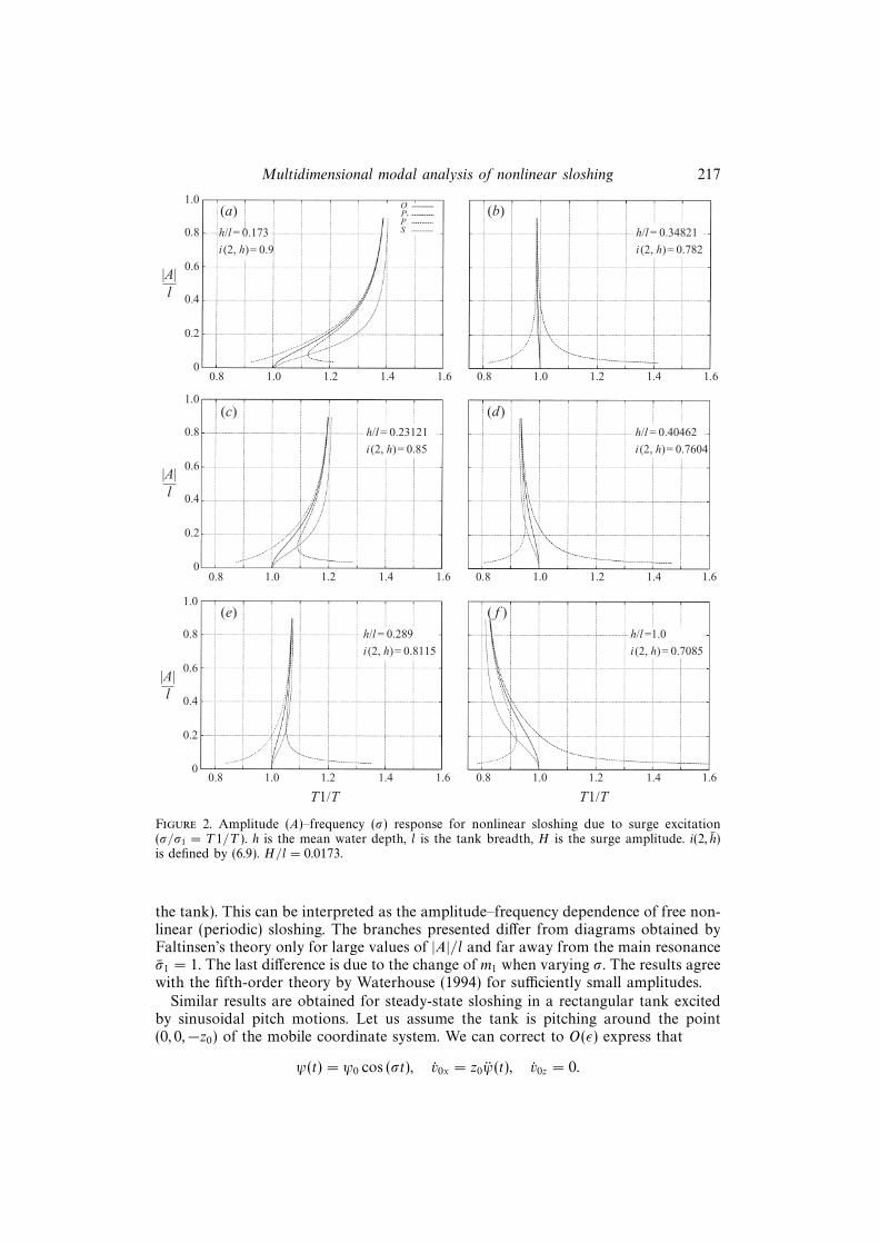
Figure 2 shows the positive and negative solutions (branches P+, P−) of the secularalgebraic equation (6.5) for different values of the water depth h and fixed amplitudeof excitation H . The choice of H corresponds to the experimental values reportedlater in the paper. Branch O is the set of solutions of (6.5) for H = 0 (no vibration of
Multidimensional modal analysis of nonlinear sloshing 217
1.0
0.8
0.6
0.4
0.2
00.8 1.0 1.2 1.4 1.6 0.8 1.0 1.2 1.4 1.6
|A|l
h/l = 0.173
i (2, h)= 0.9
OP+P–S h/l = 0.34821
i (2, h)= 0.782
1.0
0.8
0.6
0.4
0.2
0
|A|l
0.8 1.0 1.2 1.4 1.6 0.8 1.0 1.2 1.4 1.6
h/l = 0.23121
i (2, h)= 0.85
h/l = 0.40462
i (2, h)= 0.7604
1.0
0.8
0.6
0.4
0.2
0
|A|l
0.8 1.0 1.2 1.4 1.6 0.8 1.0 1.2 1.4 1.6
h/l = 0.289
i (2, h)= 0.8115
h/l =1.0
i (2, h)= 0.7085
T1/T T1/T
(a) (b)
(c) (d)
(e) ( f )
Figure 2. Amplitude (A)–frequency (σ) response for nonlinear sloshing due to surge excitation(σ/σ1 = T1/T ). h is the mean water depth, l is the tank breadth, H is the surge amplitude. i(2, h)is defined by (6.9). H/l = 0.0173.
the tank). This can be interpreted as the amplitude–frequency dependence of free non-linear (periodic) sloshing. The branches presented differ from diagrams obtained byFaltinsen’s theory only for large values of |A|/l and far away from the main resonanceσ1 = 1. The last difference is due to the change of m1 when varying σ. The results agreewith the fifth-order theory by Waterhouse (1994) for sufficiently small amplitudes.
Similar results are obtained for steady-state sloshing in a rectangular tank excitedby sinusoidal pitch motions. Let us assume the tank is pitching around the point(0, 0,−z0) of the mobile coordinate system. We can correct to O(ε) express that
ψ(t) = ψ0 cos (σt), v0x = z0ψ(t), v0z = 0.

218 O. M. Faltinsen, O. F. Rognebakke, I. A. Lukovsky and A. N. Timokha
1.0
0.8
0.6
0.4
0.2
00.8 1.0 1.2 1.4 1.6 0.8 1.0 1.2 1.4 1.6
|A|l
ã0= 0.1 rad
OP+P–S
1.0
0.8
0.6
0.4
0.2
0
|A|l
0.8 1.0 1.2 1.4 1.6 0.8 1.0 1.2 1.4 1.6
1.0
0.8
0.6
0.4
0.2
0
|A|l
0.8 1.0 1.2 1.4 1.6 0.8 1.0 1.2 1.4 1.6
T1/T T1/T
(a) (b)
(c) (d)
(e) ( f )
ã0= 0.2 rad
ã0= 0.1 rad ã0= 0.2 rad
ã0= 0.1 rad ã0= 0.2 rad
Figure 3. Amplitude (A)–frequency (σ) response for nonlinear sloshing due to pitch excitation(σ/σ1 = T1/T ). h is the mean water depth, l is the tank breadth, ψ0 is the pitch amplitude, (0,−z0)
is the position of pitch axis. i(2, h) is defined by (6.9). (a, b) z0/l = 0, h/l = 0.2, i(2, h) = 0.874; (c, d)
z0/l = 0.15, h/l = 0.35, i(2, h) = 0.78; (e, f) z0/l = 0.3, h/l = 0.5, i(2, h) = 0.737.
The algebraic governing equation for the frequency–amplitude response takes thefollowing form:
(σ21 − 1)A+ m1(σ2, h)A
3 − P1ψ0
(z0
l− S1
l+
g
lσ2
)= 0. (6.8)
It differs from the equation of forced surge steady-state sloshing (6.5) only by the lastinhomogeneous term and agrees with the corresponding equation of Faltinsen (1974).
All the results are based on the assumption that O(β21 ) = O(β2). However, even
for periodic solutions we can find a critical value of σ/σ1 for which the amplitude
Multidimensional modal analysis of nonlinear sloshing 219
of the second mode tends to infinity. It can happen for small h, or for σ22 → 4 (see
the asymptotic solution (6.3), (6.4)). In terms of σ the condition of the secondaryresonance takes the form
σ
σ1
→√
tanh (2πh/l)
2 tanh (πh/l)= i(2, h). (6.9)
The value i(2, h) characterizes the applicability of the theory constructed (see figures 2and 3). The ratio T1/T = σ/σ1 must be close to 1 and not close to i(2, h).
Similarly, we can introduce for the third mode
i(3, h) =
√tanh (3πh/l)
3 tanh (πh/l). (6.10)
However since i(3, h) < i(2, h), the secondary resonance is the most dangerous.The trend of the distribution of i(2, h) shows for h small enough (but large for
shallow water theory) that i(2, h) → 1 as h → 0. This means that the secondaryparametric resonance can occur for small depths and implies that the asymptotictheory presented is not applicable for shallow water.
The stability analysis for surge/pitch excited waves in a rectangular container wasdone by Faltinsen (1974). We can give reliable new treatment of the stability byintroducing branches O and S in figures 2 and 3. The branch O is the relation for thefrequency and amplitude for nonlinear free sloshing, which can be found from theequation
branch O: (σ21 − 1) + m1(σ2, h)A
2 = 0. (6.11)
The branch O is also the asymptotic curve for P− and P+ as A→∞.The branch S is the set of all turning points of the branch P+ (or P− for different
depths) for various amplitudes H (surge excitation) or ψ0 (pitch excitation). Theturning points correspond to when (6.5) has only two solutions. The condition of tworoots of equation (6.5) can be found by differentiating (6.5) with respect to A. This gives
branch S: (σ21 − 1) + 3m1(σ2, h)A
2 = 0. (6.12)
The branch S does not depend on the value of the excitation amplitude and is onlya function of depth–breadth ratio.
Due to the theory of bifurcations the turning point divides the branch P+ or P− intostable and unstable sub-branches. It was shown by Faltinsen (1974) that the uppersub-branch of P+/P− corresponds to unstable solutions and the lower sub-branch tostable solutions. The branch P−/P+ without a turning point corresponds to stablesolutions. When repeating the averaging asymptotic analysis given by Faltinsen forour solutions, we arrive at the same result if A 1.
When varying the values of the excitation amplitude, the sub-branch situatedbetween S and O will always correspond to unstable solutions.
7. Comparison between theory and experimentsA series of experiments on nonlinear sloshing in a smooth rectangular tank due
to horizontal (surge) excitation were conducted. Figure 4 shows the tank used in theexperiments. The tank has a front plate made of Plexiglas which is stiffened by twovertical L-beams. The tank was placed on a wagon that could slide back and forth
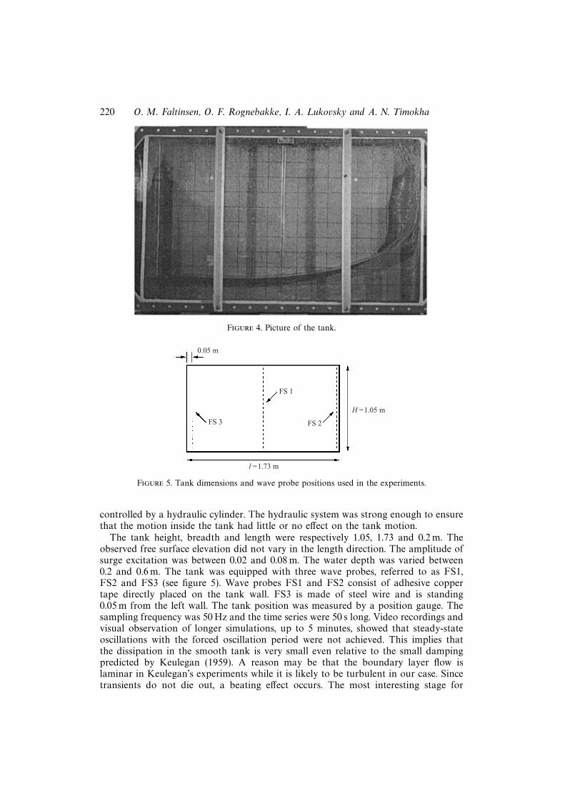
220 O. M. Faltinsen, O. F. Rognebakke, I. A. Lukovsky and A. N. Timokha
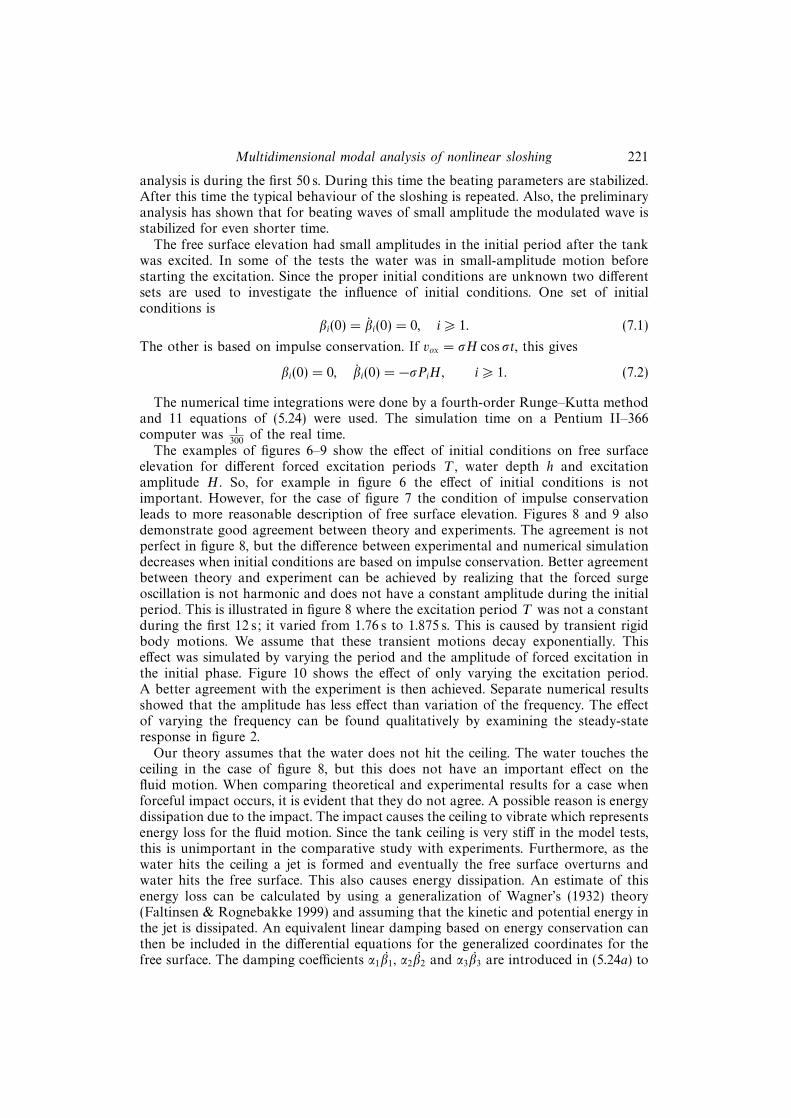
Figure 4. Picture of the tank.
0.05 m
FS 3
FS 1
FS 2
l =1.73 m
H =1.05 m
Figure 5. Tank dimensions and wave probe positions used in the experiments.
controlled by a hydraulic cylinder. The hydraulic system was strong enough to ensurethat the motion inside the tank had little or no effect on the tank motion.
The tank height, breadth and length were respectively 1.05, 1.73 and 0.2 m. Theobserved free surface elevation did not vary in the length direction. The amplitude ofsurge excitation was between 0.02 and 0.08 m. The water depth was varied between0.2 and 0.6 m. The tank was equipped with three wave probes, referred to as FS1,FS2 and FS3 (see figure 5). Wave probes FS1 and FS2 consist of adhesive coppertape directly placed on the tank wall. FS3 is made of steel wire and is standing0.05 m from the left wall. The tank position was measured by a position gauge. Thesampling frequency was 50 Hz and the time series were 50 s long. Video recordings andvisual observation of longer simulations, up to 5 minutes, showed that steady-stateoscillations with the forced oscillation period were not achieved. This implies thatthe dissipation in the smooth tank is very small even relative to the small dampingpredicted by Keulegan (1959). A reason may be that the boundary layer flow islaminar in Keulegan’s experiments while it is likely to be turbulent in our case. Sincetransients do not die out, a beating effect occurs. The most interesting stage for
Multidimensional modal analysis of nonlinear sloshing 221
analysis is during the first 50 s. During this time the beating parameters are stabilized.After this time the typical behaviour of the sloshing is repeated. Also, the preliminaryanalysis has shown that for beating waves of small amplitude the modulated wave isstabilized for even shorter time.
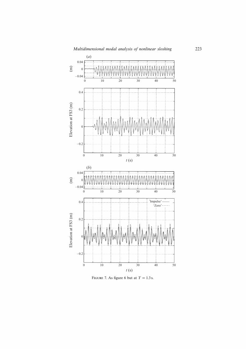
The free surface elevation had small amplitudes in the initial period after the tankwas excited. In some of the tests the water was in small-amplitude motion beforestarting the excitation. Since the proper initial conditions are unknown two differentsets are used to investigate the influence of initial conditions. One set of initialconditions is
βi(0) = βi(0) = 0, i > 1. (7.1)
The other is based on impulse conservation. If vox = σH cos σt, this gives
βi(0) = 0, βi(0) = −σPiH, i > 1. (7.2)
The numerical time integrations were done by a fourth-order Runge–Kutta methodand 11 equations of (5.24) were used. The simulation time on a Pentium II–366computer was 1
300of the real time.
The examples of figures 6–9 show the effect of initial conditions on free surfaceelevation for different forced excitation periods T , water depth h and excitationamplitude H . So, for example in figure 6 the effect of initial conditions is notimportant. However, for the case of figure 7 the condition of impulse conservationleads to more reasonable description of free surface elevation. Figures 8 and 9 alsodemonstrate good agreement between theory and experiments. The agreement is notperfect in figure 8, but the difference between experimental and numerical simulationdecreases when initial conditions are based on impulse conservation. Better agreementbetween theory and experiment can be achieved by realizing that the forced surgeoscillation is not harmonic and does not have a constant amplitude during the initialperiod. This is illustrated in figure 8 where the excitation period T was not a constantduring the first 12 s; it varied from 1.76 s to 1.875 s. This is caused by transient rigidbody motions. We assume that these transient motions decay exponentially. Thiseffect was simulated by varying the period and the amplitude of forced excitation inthe initial phase. Figure 10 shows the effect of only varying the excitation period.A better agreement with the experiment is then achieved. Separate numerical resultsshowed that the amplitude has less effect than variation of the frequency. The effectof varying the frequency can be found qualitatively by examining the steady-stateresponse in figure 2.
Our theory assumes that the water does not hit the ceiling. The water touches theceiling in the case of figure 8, but this does not have an important effect on thefluid motion. When comparing theoretical and experimental results for a case whenforceful impact occurs, it is evident that they do not agree. A possible reason is energydissipation due to the impact. The impact causes the ceiling to vibrate which representsenergy loss for the fluid motion. Since the tank ceiling is very stiff in the model tests,this is unimportant in the comparative study with experiments. Furthermore, as thewater hits the ceiling a jet is formed and eventually the free surface overturns andwater hits the free surface. This also causes energy dissipation. An estimate of thisenergy loss can be calculated by using a generalization of Wagner’s (1932) theory(Faltinsen & Rognebakke 1999) and assuming that the kinetic and potential energy inthe jet is dissipated. An equivalent linear damping based on energy conservation canthen be included in the differential equations for the generalized coordinates for thefree surface. The damping coefficients α1β1, α2β2 and α3β3 are introduced in (5.24a) to

222 O. M. Faltinsen, O. F. Rognebakke, I. A. Lukovsky and A. N. Timokha
0.04
–0.04
0
0 10 20 30 40 50
(a)
(b)
(m)
0 10 20 30 40 50
0.4
0.2
0
–0.2
0.04
0
–0.040 10 20 30 40 50
(m)
0 10 20 30 40 50
0.4
0.2
0
–0.2
Ele
vati
on a
t FS
3 (m
)E
leva
tion
at F
S3
(m)
t (s)
t (s)
‘Impulse’‘Zero’
Figure 6. (a) Measured and (b) calculated tank position and free surface elevation at wave probeFS3 (h = 0.6 m, T = 1.5 s). The curve ‘Zero’ corresponds to zero initial conditions, ‘Impulse’ meansinitial impulse condition.
Multidimensional modal analysis of nonlinear sloshing 223
0.04
–0.04
0
0 10 20 30 40 50
(a)
(b)
(m)
0 10 20 30 40 50
0.4
0.2
0
–0.2
0.04
0
–0.04
0 10 20 30 40 50
(m)
0 10 20 30 40 50
0.4
0.2
0
–0.2
Ele
vati
on a
t FS
3 (m
)E
leva
tion
at F
S3
(m)
t (s)
t (s)
‘Impulse’‘Zero’
Figure 7. As figure 6 but at T = 1.3 s.

224 O. M. Faltinsen, O. F. Rognebakke, I. A. Lukovsky and A. N. Timokha
0.04
–0.04
0
0 10 20 30 40 50
(a)
(b)
(m)
0 10 20 30 40 50
0.4
0.2
0
–0.2
0.04
0
–0.04
0 10 20 30 40 50
(m)
0 10 20 30 40 50
0.4
0.2
0
–0.2
Ele
vati
on a
t FS
3 (m
)E
leva
tion
at F
S3
(m)
t (s)
t (s)
‘Impulse’‘Zero’
Figure 8. As figure 6 but at h = 0.5 m, T = 1.875 s.

Multidimensional modal analysis of nonlinear sloshing 225
0.04
–0.04
0
0 10 20 30 40 50
(a)
(b)
(m)
0 10 20 30 40 50
0.4
0.2
0
–0.2
0.04
0
–0.040 10 20 30 40 50
(m)
0 10 20 30 40 50
0.4
0.2
0
–0.2
Ele
vati
on a
t FS
3 (m
)E
leva
tion
at F
S3
(m)
t (s)
t (s)
‘Impulse’‘Zero’
Figure 9. As figure 6 but at h = 0.5 m, T = 1.4 s.

226 O. M. Faltinsen, O. F. Rognebakke, I. A. Lukovsky and A. N. Timokha
0.04
–0.04
0
0 10 20 30 40 50(m
)
0 10 20 30 40 50
0.4
0.2
0
–0.2
1.88
0 10 20 30 40 50
(m)
Ele
vati
on a
t FS
3 (m
)
t (s)
1.84
1.80
1.76
‘Impulse’‘Zero’
Figure 10. Calculated tank position and free surface elevation at wave probe FS3 for h = 0.5 m.Effect of varying excitation period exponentially from 1.77 s to 1.875 s.
(5.24c), respectively. Since the average forced excitation is close to the lowest naturalfrequency, it is only α1 that matters. Figure 11 shows satisfactory agreement betweentheory and experiments by including damping. The damping will vary from cycleto cycle depending on the severity of the water impact. In the presented case wecalculated approximately 40% loss of energy in the tank for every cycle due to thetwo impacts occurring.
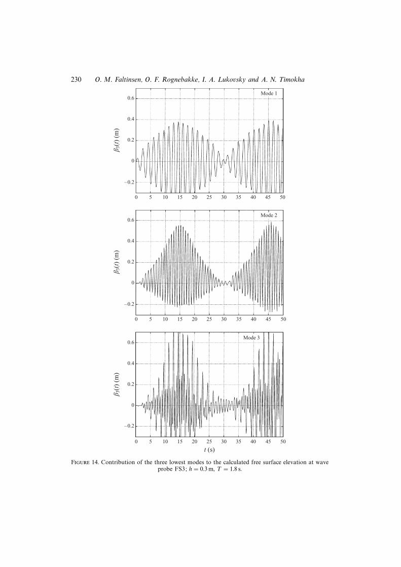
The theory will break down for small water depth. Figure 12 presents experimentaldata and numerical simulation for h/l = 0.173 and T1/T = 0.96. Since i2 = 0.9,the effect of secondary parametric resonance is important. We note that the wavecrest is well predicted, while the theoretical value for the trough is clearly lowerthan in the experiments. In order to improve the theoretical predictions we haveto assume that at least the two lowest modes have the same order of magnitude.This means a complete change of the equation system and higher modes have tobe introduced in the nonlinear equations. The introduction of the fourth mode inthe nonlinear equation system will affect the difference between trough and crest sothat the agreement with experiments may improve. The difference between theoryand experiments is more evident in figure 13 where T1/T = 1.17 and h/l = 0.173.The reason is once again that the primary mode is not dominating. This contradictsour theoretical assumptions. Figure 14 shows that the amplitude of the third mode ishigher than the second mode, which is higher than the first mode.

Multidimensional modal analysis of nonlinear sloshing 227
Ele
vati
on a
t FS
3 (m
)
t (s)
0.8
0.6
0.4
0.2
0
–0.2
–0.40 5 10 15
ExperimentTheory
Figure 11. Measured and calculated free surface elevation at wave probe FS3 for T = 1.71 s,h = 0.5 m and H = 0.05 m. Calculations account for wave impact on tank ceiling.
8. Calculations of hydrodynamic loads on the tankHow to calculate hydrodynamic loads will be illustrated for the surge-excited
rectangular tank. The general expression for the pressure is given by (2.5). By notingthat Φ = v0xx+ ϕ and by expressing v0x as −Hσ sin (σt) it follows that
p = p0 − ρ[∂ϕ
∂t+ 1
2(∇ϕ)2 + gz − σ2H cos (σt)x− 1
2H2σ2 sin2 (σt)
]. (8.1)
Here we use
∇ϕ =
N∑i=1
iπ
lRi(t)
(− sin
(iπ
l
(x+
l
2
))cosh ((iπ/l)(z + h))
cosh ((iπ/l)h), 0,
cos
(iπ
l
(x+
l
2
))sinh ((iπ/l)(z + h))
cosh ((iπ/l)h)
), (8.2)
∂ϕ
∂t=
N∑i=1
Ri(t) cos
(iπ
l
(x+
l
2
))cosh ((iπ/l)(z + h))
cosh ((iπ/l)h), (8.3)
where Ri and Ri are calculated by (5.12) and (5.13) and N is a number of Fourierterms (N > 3). When applying these formulas above the mean free surface, a Taylorexpansion about the mean free surface has to be used.
The force F on the tank due to the fluid can be calculated by direct pressureintegration or the compact formula derived by Lukovsky (1990)
F = mlg− ml[v0 + ω × v0 + ω × (ω × r1C) + ω × r1C + 2ω × r1C + r1C] (8.4)
where r1C is radius-vector of the mass centre in mobile coordinate system Oxyz andml is fluid mass. We note that F includes the static force component mlg in additionto hydrodynamic forces.
The formula takes the form
F = mlg− ml(v0 + r1C) (8.5)
in the absence of angular motions (ω = 0).

228 O. M. Faltinsen, O. F. Rognebakke, I. A. Lukovsky and A. N. Timokha
0.04
–0.04
0
0 10 20 30 40 50
(a)
(b)
(m)
0 10 20 30 40 50
0.4
0.2
0
–0.2
0.04
0
–0.04
0 10 20 30 40 50
(m)
0 10 20 30 40 50
0.4
0.2
0
–0.2
Ele
vati
on a
t FS
3 (m
)E
leva
tion
at F
S3
(m)
t (s)
t (s)
‘Impulse’‘Zero’
0.6
0.6
Figure 12. (a) Measured and (b) calculated tank position and free surface elevation at wave probeFS3 (h = 0.3 m, T = 2.2 s).

Multidimensional modal analysis of nonlinear sloshing 229
0.04
–0.04
0
0 10 20 30 40 50
(a)
(b)
(m)
0 10 20 30 40 50
0.4
0.2
0
–0.2
0.04
0
–0.04
0 10 20 30 40 50
(m)
0 10 20 30 40 50
0.4
0.2
0
–0.2
Ele
vati
on a
t FS
3 (m
)E
leva
tion
at F
S3
(m)
t (s)
t (s)
‘Impulse’‘Zero’
0.6
0.6
Figure 13. As figure 12 but at T = 1.8 s.
230 O. M. Faltinsen, O. F. Rognebakke, I. A. Lukovsky and A. N. Timokha
0.6
0.4
0.2
0
–0.2
0 5 10 15 20 25 30 35 40 45 50
Mode 1
b 3(t
) (m
)
0.6
0.4
0.2
0
–0.2
0 5 10 15 20 25 30 35 40 45 50
b 3(t
) (m
)
0.6
0.4
0.2
0
–0.2
0 5 10 15 20 25 30 35 40 45 50
b 3(t
) (m
)
Mode 3
Mode 2
t (s)
Figure 14. Contribution of the three lowest modes to the calculated free surface elevation at waveprobe FS3; h = 0.3 m, T = 1.8 s.

Multidimensional modal analysis of nonlinear sloshing 231
–0.26
–0.27
–0.28
–0.29
–0.30–0.2 –0.1 0 0.1 0.2
x (m)
z (m
)
Figure 15. The position of mass centre for the case in figure 6.
The calculation shows, that if r1C = (xC(t), 0, zC(t)), then
xC = − l
π2h
N∑i=1
βi(t)1
i2(1 + (−1)i+1), zC = −h
2+
1
4h
n∑i=1
β2i (t), (8.6)
where the point (0,−h/2) corresponds to mass centre of unperturbed fluid.By introducing the vector F = (Fx, 0, Fz) we arrive at
Fx/ml =
(Hσ2 cos σt+
l
π2h
N∑i=1
βi(t)1
i2(1 + (−1)i+1)
),
Fz/ml = −(g +
1
2h
N∑i=1
(βiβi + β2i )
).
(8.7)
Figure 15 shows the trajectory of the mass centre. Figure 16 presents the trajectoryof the end of the vector F /ml .
The hydrodynamic moment N on the tank can also be calculated by the specialformula derived by Lukovsky (1990) (moment axis coincides with Oy)
N = mlr1C × (g− ω × v0 − v0)− J1 · ω − J1 · ω − ω × (J1 · ω)
−lω + lωt − ω × (lω − lωt), (8.8)
where the inertia tensor J1 is defined by (3.13) and lω, lωt by (3.15).For ω = 0
N = ml r1C × (g− v0)− lω + lωt. (8.9)
The time-varying functions lω, lωt depend on the solutions of the Neumann boundaryvalue problem (3.5) and can be expressed mathematically like the Stokes–Zhukovskypotentials.
By using Green’s formula we get
N(t) = ml(xCg − zCv0)− ρ d
dt
∫S+Σ
(zν1 − xν3)ϕ dS, (8.10)
where N = (0, N(t), 0).
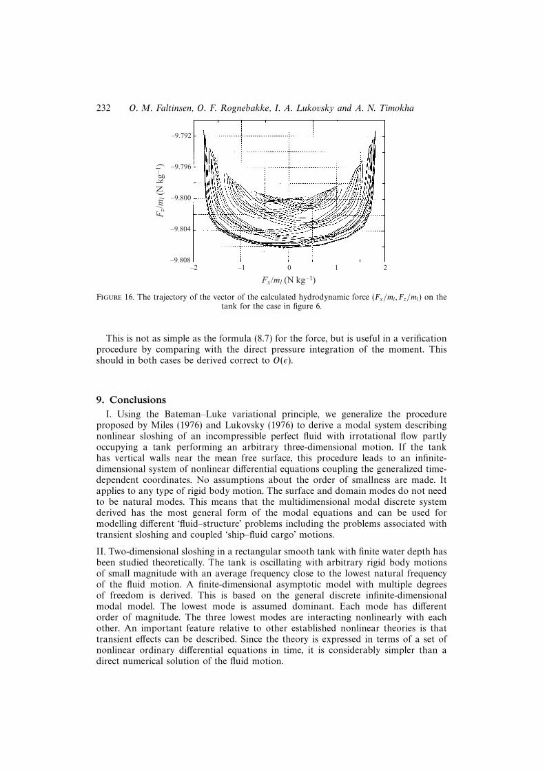
232 O. M. Faltinsen, O. F. Rognebakke, I. A. Lukovsky and A. N. Timokha
–9.792
–2 –1 0 1 2
Fx/ml (N kg–1)
Fz/
ml (
N k
g–1
) –9.796
–9.800
–9.804
–9.808
Figure 16. The trajectory of the vector of the calculated hydrodynamic force (Fx/ml, Fz/ml) on thetank for the case in figure 6.
This is not as simple as the formula (8.7) for the force, but is useful in a verificationprocedure by comparing with the direct pressure integration of the moment. Thisshould in both cases be derived correct to O(ε).
9. ConclusionsI. Using the Bateman–Luke variational principle, we generalize the procedure
proposed by Miles (1976) and Lukovsky (1976) to derive a modal system describingnonlinear sloshing of an incompressible perfect fluid with irrotational flow partlyoccupying a tank performing an arbitrary three-dimensional motion. If the tankhas vertical walls near the mean free surface, this procedure leads to an infinite-dimensional system of nonlinear differential equations coupling the generalized time-dependent coordinates. No assumptions about the order of smallness are made. Itapplies to any type of rigid body motion. The surface and domain modes do not needto be natural modes. This means that the multidimensional modal discrete systemderived has the most general form of the modal equations and can be used formodelling different ‘fluid–structure’ problems including the problems associated withtransient sloshing and coupled ‘ship–fluid cargo’ motions.
II. Two-dimensional sloshing in a rectangular smooth tank with finite water depth hasbeen studied theoretically. The tank is oscillating with arbitrary rigid body motionsof small magnitude with an average frequency close to the lowest natural frequencyof the fluid motion. A finite-dimensional asymptotic model with multiple degreesof freedom is derived. This is based on the general discrete infinite-dimensionalmodal model. The lowest mode is assumed dominant. Each mode has differentorder of magnitude. The three lowest modes are interacting nonlinearly with eachother. An important feature relative to other established nonlinear theories is thattransient effects can be described. Since the theory is expressed in terms of a set ofnonlinear ordinary differential equations in time, it is considerably simpler than adirect numerical solution of the fluid motion.

Multidimensional modal analysis of nonlinear sloshing 233
Periodic solutions are studied analytically. The amplitude–frequency response isconsistent with the fifth-order steady-state solution by Waterhouse (1994).
It is shown that the theory is not valid when the water depth (h) becomes smallrelative to the tank breadth (l). This is due to secondary parametric resonance. Itis then necessary to include nonlinearly interacting modes having the same order ofmagnitude. This is demonstrated for a tank with h/l = 0.173.
III. We have conducted experimental studies of the free surface elevation for forcedsurge oscillations of two-dimensional flow in a rectangular tank. It is demonstratedexperimentally that it takes a very long time for transient fluid motion to die out.This did not occur during an observation period of 5 minutes, which corresponds tothe order of 150–200 oscillations in terms of the excitation period. The consequenceis that steady-state solutions of nonlinear sloshing in a smooth tank can have limitedapplicability. Modulated (‘beating’) waves occurred as a consequence of transient andforced oscillations. The amplitude/‘beating’ period was stabilized during the first 50 s.
Since we could not exactly state what the initial conditions were in the experiments,a sensitivity study was performed with different initial conditions in the theoreticalmodel. The results were not strongly dependent on this, but better agreement betweentheory and experiments was in general obtained by using an initial condition based onimpulse conservation. For several experiments we observed fluctuations of the excita-tion frequency in an initial period up to approximately 10 s. This effect was importantto include in the theoretical model. There is good agreement with experimental freesurface elevation when h/l > 0.28.
IV. The theory was compared with experiments when forceful water impact on thetank ceiling occurred. The theory assumes no tank ceiling. The experimental freesurface elevations showed a clear influence of the water impact. It was speculatedthat this was due to energy dissipation and phenomenological linear damping termswere introduced in the discrete modal system. Good agreement with the experimentswas demonstrated. This is an area of future research.
V. It is shown how hydrodynamic forces on the tank can be calculated in a simpleway. An alternative formula for the hydrodynamic moment is also presented. Theform of the expressions facilities simulations of a coupled ‘vehicle–fluid’ system.
This work is supported in part by NATO Research Fellowship (Research Councilof Norway) at Norwegian University of Science and Technology, Trondheim (fourthauthor), German Research Council (D.F.G.) (third author). The work by the secondauthor is supported by the Research Council of Norway. The experimental studieswere sponsored by Det Norske Veritas.
REFERENCES
Bateman, H. 1944 Partial Differential Equations of Mathematical Physics. Dover.
Buechmann, B. A. 1996 2D numerical wave based on a third order boundary element model. In 9thConf. European Consortium for Mathematics in Industry, Lyngby/Copenhagen, Denmark, June25–27, 1996, pp. 417–420.
Chen, Sh., Johnson, D. B., Raad, P. E. & Fadda, D. 1997 Surface marker and micro cell method.Intl J. Numer. Meth. Fluids 25, 749–778.
Dodge, F. T., Kana, D. D. & Abramson, H. N. 1965 Liquid surface oscillations in longitudinallyexcited rigid cylindrical containers. AIAA J. 3, 685–695.
Faltinsen, O. M. 1974 A nonlinear theory of sloshing in rectangular tanks. J. Ship. Res. 18,224–241.

234 O. M. Faltinsen, O. F. Rognebakke, I. A. Lukovsky and A. N. Timokha
Faltinsen, O. M. & Rognebakke, O. F. 1999 Sloshing and slamming in tanks. In Hydronav’99.–Manoeuvering’99 Gdansk – Ostroda, 1999, Poland. Technical University of Gdansk.
Funakoshi, M. & Inoue S. 1991 Bifurcations in resonantly forced water waves. Eur. J. Mech.B/Fluids. 10, 31–36.
Hargneaves, R. 1908 A pressure–integral as kinetic potential. Phil. Mag. 16, 436–444.
Ikeda, T. & Nakagawa, N. 1997 Non-linear vibrations of a structure caused by water sloshing ina rectangular tank. J. Sound Vib. 201, 23–41.
Keulegan, G. H. 1959 Energy dissipation in standing waves in rectangular basin. J. Fluid Mech. 6,33–50.
Limarchenko, O. S. & Yasinsky, V. V. 1997 Nonlinear Dynamics of Constructions with a Fluid. KievPolytechnic University (in Russian).
Luke, J. C. 1967 A variational principle for a fluid with a free surface. J. Fluid Mech. 27, 395–397.
Lukovsky, I. A. 1976 Variational method in the nonlinear problems of the dynamics of a limitedliquid volume with free surface. In Oscillations of Elastic Constructions with Liquid, pp. 260–264Moscow: Volna (in Russian).
Lukovsky, I. A. 1990 Introduction to Nonlinear Dynamics of a Solid Body with a Cavity including aLiquid. Kiev: Naukova dumka (in Russian).
Lukovsky, I. A. & Timokha, A. N. 1995 Variational Methods in Nonlinear Dynamics of a LimitedLiquid Volume. Kiev: Institute of Mathematics (in Russian).
Mikishev, G. I. 1978 Experimental methods in the dynamics of spacecraft. Moscow: Mashinostroenie(in Russian).
Miles, J. W. 1976 Nonlinear surface waves in closed basins. J. Fluid Mech. 75, 419–448.
Miles, J. W. 1984a Internally resonant surface waves in a circular cylinder. J. Fluid Mech. 149, 1–14.
Miles, J. W. 1984b Resonantly forced surface waves in a circular cylinder. J. Fluid Mech. 149, 15–31.
Moan, T. & Berge, S. (Eds.) 1997 Report of Committee 1.2 “Loads”. In Proc. 13th Intl Ship andOffshore Structures Congress, Vol. 1, pp. 59–122. Pergamon.
Moiseev, N. N. 1958 To the theory of nonlinear oscillations of a limited liquid volume of a liquid.Prikl. Math. Mech. 22, 612–621 (in Russian).
Narimanov, G. S. 1957 Movement of a tank partly filled by a fluid: the taking into account ofnon-smallness of amplitude. Prikl. Math. Mech. 21, 513–524 (in Russian).
Narimanov, G. S., Dokuchaev, L. V. & Lukovsky, I. A. 1977 Nonlinear Dynamics of FlyingApparatus with Liquid. Moscow: Mashinostroenie (in Russian).
Pawell, A. 1997 Free Surface Waves in A Wave Tank. Intl Series Numer. Maths 124, 311–320.Birkhauser.
Pilipchuk, V. N. & Ibrahim, P. A. 1997 The dynamics of non–linear system simulating liquidsloshing impact in moving structures. J. Sound Vib. 205, 593–615.
Shemer, L. 1990 On the directly generated resonant standing waves in a rectangular tank. J. FluidMech. 217, 143–165.
Solaas, F. & Faltinsen, O. M. 1997 Combined numerical and analytical solution for sloshing intwo-dimensional tanks of general shape. J. Ship Res. 41, 118–129.
Su Tsung-Chow 1992 Nonlinear sloshing and the coupled dynamics of liquid propellants andspacecraft. NASA Tech. Rep. AD-A250023.
Tanizawa, K. 1996 A nonlinear simulation method of 3D body motions in waves extendedformulation for multiple fluid domains. In 11th Intl Workshop on Water Waves and FloatingBodies, March 1996, Hamburg, Germany. Abstracts.
Tsai, W.-T., Yue, D. K.-P. & Yip, K. M. K. 1990 Resonantly excited regular and chaotic motions ina rectangular wave tank. J. Fluid Mech. 216, 343–380.
Verhagen, J. H. G. & Wijngaarden, L. van 1965 Nonlinear oscillations of fluid in a container. J.Fluid Mech. 22, 737–751.
Wagner, H. 1932 Uber Stoss- und Gleitvorgange an der Oberflache von Flussigkeiten. Z. Angew.Math. Mech. 12, 193–235.
Waterhouse, D. D. 1994 Resonant sloshing near a critical depth. J. Fluid Mech. 281, 313–318.