Accepted Manuscript

Multidimensional extension of the continuity equation method for debris cloudsevolution

Francesca Letizia, Camilla Colombo, Hugh G. Lewis

PII: S0273-1177(15)00832-7DOI: http://dx.doi.org/10.1016/j.asr.2015.11.035Reference: JASR 12538

To appear in: Advances in Space Research

Received Date: 31 October 2014Revised Date: 26 October 2015Accepted Date: 27 November 2015

Please cite this article as: Letizia, F., Colombo, C., Lewis, H.G., Multidimensional extension of the continuityequation method for debris clouds evolution, Advances in Space Research (2015), doi: http://dx.doi.org/10.1016/j.asr.2015.11.035

This is a PDF file of an unedited manuscript that has been accepted for publication. As a service to our customerswe are providing this early version of the manuscript. The manuscript will undergo copyediting, typesetting, andreview of the resulting proof before it is published in its final form. Please note that during the production processerrors may be discovered which could affect the content, and all legal disclaimers that apply to the journal pertain.

Multidimensional extension of the continuity equationmethod for debris clouds evolution

Francesca Letizia∗

Astronautics Research Group,University of Southampton, Southampton, UK

Camilla Colombo

Department of Aerospace Science and Technology, Politecnico di Milano, Milano, Italy

Hugh G. Lewis

Astronautics Research Group,University of Southampton, Southampton, UK

Abstract

As the debris spatial density increases due to recent collisions and inoperative

spacecraft, the probability of collisions in space grows. Even a collision involv-

ing small objects may produce thousands of fragments due to the high orbital

velocity and the high energy released. The propagation of the trajectories of all

the objects produced by a breakup would be prohibitive in terms of computa-

tional time; therefore, simplified models are needed to describe the consequences

of a collision with a reasonable computational effort. The continuity approach

can be applied to this purpose as it allows switching the point of view from the

analysis of each single fragment to the study of the evolution of the debris cloud

globally. Previous formulations of the continuity equation approach focussed on

the representation of the drag effect on the fragment spatial density. This work

proposes how the continuity equation approach can be extended to multiple

dimensions in the phase space defined by the relevant orbital parameters. This

novel approach allows including in the propagation also the effect of the Earth’s

oblateness and improving the description of the drag effect by considering the

∗Corresponding authorEmail address: f.letizia@soton.ac.uk (Francesca Letizia)

Preprint submitted to Advances in Space Research December 8, 2015

distribution of area-to-mass ratio and eccentricity among the fragments. Re-

sults for these three applications are shown and discussed in terms of accuracy

compared to the numerical propagation and to the one-dimensional approach.

Keywords: space debris, continuity equation, debris cloud, fragments

propagation

1. Introduction

More than 17000 objects larger than 5 cm are in orbit around the Earth

and are constantly tracked from the Earth to avoid collisions for operational

satellites (IADC Steering Committee, 2013)1. The population of centimetre-

sized objects can be statistically derived from radar data and the number of

even smaller objects is inferred from impact records (Xu et al., 2009). Even if

these small objects are not catalogued individually, they can still be dangerous.

Any object larger than 1 cm is supposed to be able to destroy a satellite in case

of collision (McKnight et al., 2014) and objects as small as 1 mm can cause

relevant anomalies on spacecraft operations, leading sometime to the failure of

the mission. In addition, small fragments are usually not included in studies on

the long term evolution of debris population because their number is so large

(i.e., more than several hundred of thousands objects larger than 1 cm) that the

computational time would be prohibitive. On the other hand, excluding small

objects from these analyses may result in underestimating the collision risk or in

misinterpreting the effect of mitigation and remediation measures (White and

Lewis, 2014).

Including small fragments in debris models demands the development of

simplified approaches to describe fragment cloud evolution in a reasonable com-

putational time. Analytical models can be used to this purpose; they have been

proposed mainly for short term analysis (Hoots and Hansen, 2014) or for the

Geosynchronous Earth Orbit (GEO) region (Valk et al., 2009; Izzo, 2002), where

1The catalogued objects can be checked at https://www.space-track.org: currently,17141 objects are present in the catalogue, out of which 4054 are active.

2

the forces admit a Hamiltonian representation. Only one fully analytical model,

proposed by McInnes (1993), appears to be applicable to Low Earth Orbits

(LEO), where the debris density is the highest. The main idea of this approach

is to consider the debris population as a fluid with continuous properties, whose

density changes under the effect of drag and collisions. In this way, the analysis

of the single object is abandoned and the fragment density is used as the only

parameter of interest.

The evolution of the density is obtained through the continuity equation, a

traditional approach in fluid-dynamics, where it is used to link the fluid density

with its velocity. Similarly, when applied in astrodynamics, it allows describing

the change in the density of a dispersed set starting from the knowledge of the

velocities of the particles. In particular, if n represents the fragment density,

the continuity equation can be written as

∂n

∂t+∇ • f = n+ − n− (1)

where ∇ • f models the forces acting on the system and accounts for slow/ con-

tinuous phenomena (such as perturbations) and n+− n− represents the sources

and the sinks of the system, so it can models fast/discontinuous events (e.g.,

the injection of new fragments due to launches). Once the initial distribution

of n is known, the continuity equation is used to obtain its evolution with time,

with very low computational effort.

The method is general and it has been applied also to describe the evolution

of interplanetary dust (Gor’kavyi, 1997; Gor’kavyi et al., 1997), nano-satellites

constellations (McInnes, 2000) and high area-to-mass spacecraft (Colombo and

McInnes, 2011). In all these cases, continuous and/or discontinuous phenomena

have to be described, as summarised in Table 1.

One can observe from Table 1 that the continuity equation can be used to find

the evolution of the system both in the physical space (such as in the examples

on space debris and nanosatellites, where the variables of the problem are time

and distance from Earth) and in the phase space (such as in the examples on

3

interplanetary dust and high area-to-mass ratio objects, where orbital elements

are used to represent the solution space). This makes the method very flexible

as it is possible to describe the evolution of the studied system in the relevant

space with the simplest formulation.

The formulation with the continuity equation is comparable to the one by

Nazarenko (1997) and Smirnov et al. (2001), who describe the evolution of the

debris population through the equation

∂Nj∂t

= −Wj∂Nj∂r−Nj

∂Wj

∂r+ Nj (2)

where Nj(r, t) is the number of debris objects in the jth bin in terms of size,

perigee altitude, eccentricity, inclination, ballistic coefficient. Wj is the radial

velocity of the objects and Nj is the rate of variation in the number of objects

due to external causes. It is easy to recognise the connection between Equation 2

and Equation 1, considering that the second and the third term in Equation 2

can be obtained from Equation 1 considering the dependence on the radial

distance only and writing the divergence in cartesian coordinates. Nazarenko

(2002) discussed the advantages of adopting a statistical model based on density

for space debris propagation compared to deterministic models. These include

a reduction in the computational time, the possibility of including objects of

any size and a more natural connection to the statistical nature of the problem

(i.e. fragment distribution with uncertain initial conditions).

The approach presented in this work aims to exploit these advantages for

Table 1: Summary of the applications of the continuity equation method to astrodynamics. aand e are the orbit semi-major axis and eccentricity; r is the distance from the central body; tis the time; Φ the angle between the Sun-Earth line and the direction of the orbit pericentre.

Application Solution space Slow phenomena Fast events Ref.

Interplanetary dust (a, e) Poynting-Robertson drag Gravitational scattering (Gor’kavyi, 1997)Planetary resonances Mutual collisions (Gor’kavyi et al., 1997)

Space debris (r, t) Atmospheric drag Mutual collisions (McInnes, 1993)Launches (Letizia et al., 2015a)

Nanosatellites (r, t) Atmospheric drag Launches and failures (McInnes, 2000)

High area-to-mass (e,Φ) Earth’s oblateness - (Colombo and McInnes, 2011)objects Solar radiation pressure

4

the propagation of single debris clouds, instead of the global debris population.

Moreover, the formulation in Equation 1 allows further enhancing the conve-

nience of the approach by providing an analytical solution to the problem of

debris cloud evolution.

In particular, the case of debris clouds in Low Earth Orbit (LEO) is studied.

The evolution of a debris cloud under the effect of perturbations can be stud-

ied with a phased approach, which splits the evolution into three main phases

(Figure 1), each one with different geometry and different driving forces (Jehn,

1991; McKnight, 1990).

(a) Ellipsoid (b) Toroid (c) Band

Figure 1: Phases of debris cloud evolution as classified by McKnight (1990) and Jehn (1991).The simulation refers to a collision on a parent orbit with inclination equal to 30.

In the first phase, the evolution of the cloud is driven by the different energy

among the fragments. This causes the cloud to be stretched along the parent

orbit, so that the mean anomaly M is randomised within a few orbits. In this

phase, the dynamics of the system is usually studied applying the two-body

problem equations.

In the following phases, the effect of perturbations drives the cloud evolution.

The Earth’s oblateness causes the nodal precession of the orbits, resulting into

the spreading of the argument of the periapsis ω and of the longitude of the

ascending node Ω. This transforms the cloud into a band around the Earth,

limited in latitude by the value of inclination of the parent orbit (Figure 1c).

Once the band has formed, ω and Ω can be considered uniformly distributed:

as a results, the forces acting on ν, ω,Ω, as the Earth’s oblateness, are not

relevant over the long term (Rossi et al., 1998). In this phase, drag becomes

the dominant perturbation and it is possible to apply the expressions found by

5

McInnes (1993) to describe the long term evolution of the fragment density.

In a previous work (Letizia et al., 2015a), this novel approach to debris propa-

gation was validated and applied to study the evolution of debris fragment clouds

generated by collisions in LEO. The method, summarised in Section 2, is able to

model the evolution of debris clouds including all the small fragments down to

1 mm in size, with a reduced computational effort compared to the propagation

of the individual trajectories. This enabled to perform an extended analysis on

the contribution of small fragments to the collision probability (Letizia et al.,

2015b), proving that the method can be useful to evaluate the hazard posed by

small fragments to operational spacecraft.

This article shows how the analytical formulation proposed by McInnes

(1993) can be extended to more dimensions to improve the description of the

drag effect and to extend the method applicability to other phases of the cloud

evolution. In detail, Section 4 discusses the description of the effect of the

Earth’s oblateness, i.e., the evolution from the ellipsoid to the band (Figure 1).

Section 5 and Section 6 focus on possible improvements of the propagation

under the drag effect by considering, respectively, the area-to-mass ratio and

eccentricity distributions among the fragments.

2. Continuity equation method for fragmentation modelling

The continuity equation can be applied to study a single fragmentation event

by using the approach summarised in the block diagram in Figure 2: a brief de-

scription of the proposed analytical model for cloud propagation in LEO (cielo,

debris Cloud Evolution in Low Earth Orbits) is presented here, whereas an ex-

tensive explanation of each block can be found in Letizia et al. (2015a).

Breakup

model

Numerical

propagation

Position

fitting

Analytical

propagation

Band

formation

Distribution

along one orbit

Energy Fragments Cloud Density

function

Figure 2: cielo building blocks.

6

The first block is a breakup model, which generates the fragments and their

characteristics (e.g., mass, velocity) given the energy of the fragmentation event.

The NASA breakup model (Johnson and Krisko, 2001; Krisko, 2011) is used

here, considering all fragments between 1 mm and 10 cm. The second block of

the method is the numerical propagation of the fragment orbital parameters.

The numerical propagator used is PlanODyn (Planetary Orbital Dynamics), a

semi-analytical method based on averaged Gauss’ equations (Colombo, 2015).

The numerical method is applied to each fragment to obtain the evolution of its

trajectory under the effect of the atmospheric drag and of the Earth’s oblateness.

For the atmospheric drag, an exponential density model is used; for the Earth’s

oblateness, only the term J2 is considered. The numerical method is used in

this work for two purposes. Firstly, it is applied to model the phase of the cloud

evolution where the Earth’s oblateness acts as main perturbation. Secondly, the

numerical method is also used to define the baseline against which the results of

the analytical method are compared and validated. Future work will validate the

analytical model against a more detailed description of the orbital perturbations,

in particular including the effect of solar radiation pressure, which is relevant

at the altitudes considered in this study.

The time required for the band formation can be estimated starting from

the parameters of the initial orbits and the energy of the fragmentation, as done

by Ashenberg (1994). Once the band is formed, the third block, position fitting,

translates the information on each single fragment into a continuous function

that describes globally the cloud. The used function is not the simple position

distribution of the fragments, but rather it is built from the probability of finding

a fragment at a certain geocentric distance given its orbital parameters (semi-

major axis a and eccentricity e) (Kessler, 1981; Sykes, 1990). Assuming that

all fragments have the same probability and summing all their contribution, the

initial density of the cloud (n0) is defined (Letizia et al., 2015a,b).

Finally, the forth block is the analytical propagation, based on the continuity

equation (Equation 1), to obtain the long-term evolution of the cloud density.

No discontinuous events are considered, so n+−n− = 0; the term ∇•f is used to

7

model atmospheric drag, following the approach developed by McInnes (1993,

2000). Assuming the band to be spherically symmetrical, the spatial problem

can be studied through only one coordinate, the radial one. In this case, f has

only one component, fr, that is written as

fr = vrn(r, t),

where vr is the radial velocity

vr = −ε√r exp(− r −RH

H

). (3)

The parameter ε

ε =√µcDA

Mρ0, (4)

collects all the terms that do not depend on r, such as the gravitational constant

µ, and the fragment drag coefficient cD, cross-sectional area A and mass M .

RH , ρ0, H are, respectively, the fragmentation altitude and the corresponding

reference density and scale height deriving from an exponential model for the

atmosphere, whose values are here taken from Vallado (2013). The expression

for the radial velocity in Equation 4 is rigorously valid only for circular orbits,

so this formulation of the problem assumes that all the fragments are on circular

orbits. In addition, Equation 3 is further simplified approximating, in the square

root, the actual distance of the fragment with the fragmentation distance

√r ≈

√RH (5)

to obtain a full analytical solution. With these assumptions, the vector field fr

can be written as

fr = −ε√RH exp

(− r −RH

H

)n(r, t); (6)

substituting this expression into Equation 1 and writing the divergence in spher-

8

ical coordinates, the following partial differential equation is obtained

∂n

∂t+ vr

∂n

∂r+(2

rvr +

∂vr∂r

)n(r, t) = 0. (7)

Applying the method of characteristics (Evans, 1998), the partial differential

equation in Equation 7 can be transformed in the following system of Ordinary

Differential Equations (ODE)

dt

ds= 1

dr

ds= vr(r)

dn

ds= −

[2

rvr +

∂vr∂r

]n(r, t),

(8)

(9)

(10)

where s expresses a parametrisation of the characteristic lines. From Equations

8 and 9 the expression of the characteristic line is obtained

Gr(r, t) = exp(r −RH

H

)+ ε

√RHH

t; (11)

and from Equations 9 and 10 the explicit expression for the density evolution

in time can be written (McInnes, 1993, 2000),

n(r, t) =Ψexp [− r−RH

H ] + (ε√RH/H)t

−εr5/2 exp [− r−RH

H ]. (12)

The function Ψ is obtained from the initial condition n(r, t = 0) and the expres-

sion of the characteristics at the initial time t = 0

Gr(r, 0) = exp(r −RH

H

)that is inverted to obtain

ri = RH +H logGr(r, t)

9

which finally allows writing an explicit expression for Ψ

Ψ(r, t) = n(ri(r, t), 0)ri(r, t)2vr(ri(r, t)). (13)

This approach provides an accurate description of the evolution of clouds

produced by fragmentation events at altitudes higher than 800 km and for any

inclination, with a reduced computational effort with respect to of the numerical

propagation (Letizia et al., 2015a). Therefore, it can be applied to study many

different scenarios of collisions to understand, for example, which objects, in

case of fragmentation, are more likely to have a large impact on the global

collision risk for operational satellites (Letizia et al., 2015b). This was done by

applying the proposed method to compute a grid of fictitious breakups, store the

scenario evolution, and evaluate their effect on several targets without having

to simulate the fragmentations for each target spacecraft.

However, the one dimensional approach has some limits

• the numerical (semi-analytical) propagation is still required to model the

first part of the cloud evolution, where the Earth’s oblateness is the main

perturbation,

• the fragments in the cloud may have very different values of area-to-

mass ratio A/M , a parameter that largely affect their decay in the at-

mosphere, but this is not captured from the original formulation from

McInnes (1993),

• the method can be applied to fragmentation events at 800 km as at lower

altitudes the hypothesis of circular orbits in Equation 3 introduces a large

error on the evolution of the cloud density (Letizia et al., 2015a).

In this work, we address these three limits of the continuity equation ap-

proach by extending it to more than one dimension in the phase space defined

by the relevant parameters for the considered problem. Moreover, we derive

a general approach to use the continuity equation in any set of phase space

variables.

10

3. Formulation of the continuity equation in multiple dimensions

Following the approach by Gor’kavyi et al. (1997), the continuity equation

can be written in the phase space by simply writing the divergence in rectangular

coordinates. This approach is chosen because the effect of perturbations is

usually described in terms of their impact on the orbital parameters (through

Gauss’ equations). Therefore, the problem is written in the space defined by

the relevant orbital parameters to use directly the expression on the orbital

parameters variation and to avoid complex transformations to a physical 3D

space. If necessary, the results can then be translated into physical coordinates

by using expressions such as the already mentioned ones by Kessler (1981)

or Sykes (1990) which express the spatial density as a function of the orbital

parameters.

Considering m generic variables (α1, . . . , αm) and assuming that n is differ-

entiable with respect to all α everywhere, the Equation 1 can be rewritten using

the expression of the divergence in rectangular coordinates

∂n

∂t+

∂n

∂α1vα1

+ · · ·+ ∂n

∂αmvαm

+[∂vα1

∂α1+ · · ·+ ∂vαm

∂αm

]n = n+ − n−. (14)

The terms of sink and source are neglected also in this case (n+ − n− = 0), so

applying the method of characteristics the following system of ODEs is obtained

dt

ds= 1

dα1

ds= vα1

(α1, . . . , αm)

...

dαmds

= vαm(α1, . . . , αm)

dn

ds= −

[∂vα1

∂α1+ · · ·+ ∂vαm

∂αm

]n(α1, . . . , αm, t).

(15)

(16)

(17)

(18)

(19)

The characteristic lines of the problem are obtained by solving the Equa-

tions 15-18, which depend on the specific formulation of the problem (which

11

gives the actual expressions for vα1 , . . . , vαm). On the other hand, the formal

expression of n(α1, . . . , αm, t) can be written for any problem. It can be ob-

tained dividing Equation 19 by the Equations 16-18. For example, dividing by

Equation 16, the result is

dn

dα1= − 1

vα1

[∂vα1

∂α1+ · · ·+ ∂vαm

∂αm

]n

where it is possible to separate the variables, so that

dn

n= − 1

vα1

[∂vα1

∂α1

]dα1 + · · · − 1

vα1

[∂vαm

∂αm

]dα1. (20)

In the last term, dα1/vα1 can be rewritten using

dα1

vα1

=dαjvαj

,

with αj one of the m coordinates. Equation 20 becomes

dn

n= − 1

vα1

[∂vα1

∂α1

]dα1 + · · · − 1

vαm

[∂vαm

∂αm

]dα, (21)

that can be easily integrated into

log(n) = − log(vα1) + · · · − log(vαm

) + k

where k is a constant of integration. Finally,

n =K∗∏mj vαj

. (22)

K is a constant (K∗ = ek) that is obtained from the initial condition at t = 0

n0(α1, . . . , αm) = n(α1, . . . , αm, t = 0) as

K∗ = n0(α1, . . . , αm)

m∏j

vαj (α1, . . . , αm).

12

where αj indicates the function obtained by inverting the characteristic lines G

at initial time t = 0. So, for example, if from Equations 15-16 it is possible to

write the characteristic line for αj

G(αj , t) = f(αj) + g(t)

then

αj = f−1(G(αj , t)),

with f−1 inverse of f .

In the next sections, the continuity equation in multiple dimensions will be

applied to three different cases. Firstly, in Section 4 it is used to model the effect

of the Earth’s oblateness, i.e., the evolution from the ellipsoid (Figure 1a) to the

band (Figure 1c). Secondly, in Section 5 it is used to include the distribution

in area-to-mass ratio A/M of the fragments for the propagation under the drag

effect. Thirdly, in Section 6 it is used to include the distribution in eccentricity,

also in this case, for the propagation under the drag effect, once the band is

formed.

4. Modelling of the effect of the Earth’s oblateness

As discussed in the previous sections, the Earth’s oblateness is the dominant

perturbation on the fragment cloud evolution before the band formation (Fig-

ure 1). The long-term effect of zonal spherical harmonics of the second order

J2 on the orbital parameters can be written as in Vallado (2013)

Ω = −3

2J2R2E

p2n cos i (23)

ω =3

2J2R2E

p2n(2− 5

2sin2 i). (24)

where RE is the Earth’s radius, p is the semi-latus rectum of the orbit p =

a(1− e2), n is the mean motion n =√µ/a3, and i is the orbit inclination.

The continuity equation can be applied to model this phase of the cloud

13

evolution by writing the problem in the phase space defined by the semi-major

axis (a), the longitude of the ascending node (Ω) and the argument of the

perigee (ω). Three possible formulations are possible. In the first case, it is

assumed that the effect of drag can be neglected and the spreading of the cloud

is evaluated only on the angles ω and Ω. In the second case, the effect of drag is

consideridered, so that the cloud density is function not only of the two angels,

but also of the semi-major axis. Finally, a third approach is presented where

only one angle and the semi-major axis are used as variables of the problem.

4.1. Earth’s oblateness only

For simplicity, it is assumed that the effect of drag can be neglected during

the initial phase of the cloud evolution, which usually lasts a couple of months.

This assumption follows the phased approach proposed by McKnight (1990)

to study space debris cloud evolution as explained in Section 1. This approach

was adopted, for example, by Jehn (1991) and Ashenberg and Broucke (1993) to

describe how the debris cloud spreads under the effect of the Earth’s oblateness,

without considering other perturbations. Introducing the approximation that

drag can be neglected, the variation of the semi-major axis is null (va = 0).

Nevertheless, the information on the distribution of a is required to calculate

the variation of Ω and ω as in Equations 23 and 24. Introducing

λ =3

2

õJ2R

2E ,

the expressions of the variation of the parameters are

vα1 = va = 0

vα2= vΩ = − λ

a7/2cos i

vα3 = vω =λ

a7/2(2− 5

2sin2 i),

(25)

(26)

(27)

14

Since a is constant, the characteristic lines are easily found as

Ga(a, t) = a

GΩ(Ω, t) = Ω +λ

a7/2cos i t

Gω(ω, t) = ω − λ

a7/2(2− 5

2sin2 i)t

that are of the form

G(α, t) = f(α) + g(t)

as introduced in Section 2. As f , in this case for all the three variables, is simply

the identity, the expressions obtained inverting the characteristics at the initial

time are identical to the characteristics, soa = Ga(a, t)

Ω = GΩ(Ω, t)

ω = Gω(ω, t)

The density of the cloud can be written as in Equation 22

n(a,Ω, ω, t) = n0(a, Ω, ω)vΩ(a)vω(a)

vΩ(a)vω(a);

as a is constant, also vΩ and vω can be simplified and therefore

n(a,Ω, ω, t) = n0(a, Ω, ω). (28)

The dependence of Ω and ω on t is linear, so n is computed extremely easily as

it corresponds to a simple translation of the domain of the initial conditions.

4.2. Earth’s oblateness and atmospheric drag (3D)

If the drag effect is considered, the variation of the semi-major axis is not

null. As explained in Section 2, the radial velocity of a fragment due to drag

15

can be expressed as in Equation 3

vr = −ε√r exp(− r −RH

H

);

also in this case, the hypothesis of circular or quasi circular orbits is kept, so

r ≈ a. Therefore, Equation 3 can be used to express the variation of the semi-

major axis substituting r with a. The expressions for the other parameters

(Ω, ω) are unchanged with respect to Equations 26 and 27, so the system of

ODEs is

dt

ds= 1

da

ds= −ε√a exp

(− a−RH

H

)dΩ

ds= − λ

a7/2cos i

dω

ds=

λ

a7/2(2− 5

2sin i2)

dn

ds= −

[∂va∂a

+∂vΩ

∂Ω+∂vω∂ω

]n(a,Ω, ω, t).

(29)

(30)

(31)

(32)

(33)

The characteristic for a is the one already obtained for r starting from the

expression for vr as in Equation 3, so

Ga(a, t) = exp(a−RH

H

)+ ε

√RHH

t;

obtained, as before, with the approximation√a ≈ √RH .

The second characteristic of the system is obtained by dividing Equation 31

by Equation 30

dΩ

da=vΩ

va=λ

ε

exp(a−RH

H

)a4

whose solution can be expressed as

GΩ(Ω, a) = Ω− λ

εcos i

[Γ(a)− Γ(a0)

]as already obtained by McInnes (1994). We take here the occasion to write

16

explicitly Γ(a) to amend a typo in the original paper

Γ(a) =− exp

(a−RH

H

)H(2H2 +Ha+ a2

)+ r3 exp−RH

H Ei[aH

]6H3a3

where Ei(z) is the exponential integral function, defined as

Ei(z) = −∫ ∞−z

exp (−u)

udu.

As ω and Ω have the same dependence on a, also the characteristic for ω is

expressed through the function Γ and only the constant factor is different. In

particular, the expression for ω is

Gω(ω, a) = ω +λ

ε(2− 5

2sin i2)

[Γ(a)− Γ(a0)

].

Therefore, also in this case is possible to write an explicit expression for n

n(a,Ω, ω, t) = n0(a, Ω, ω)va(a)vΩ(a)vω(a)

va(a)vΩ(a)vω(a)(34)

with a = RH +H log (Ga(a, t))

Ω = GΩ(Ω, a)

ω = Gω(ω, a).

Note that here the initial condition is not simply translated across the domain,

but, as the semi-major axis decreases with time, the initial distribution is mod-

ified with time as expressed by Equation 34.

4.3. Earth’s oblateness and atmospheric drag (2D)

If the purpose of the method is to obtain the long term evolution of the

cloud, the scope of the description of the effect of the Earth’s oblateness is to

estimate when the band (Figure 1c) is formed and to have at the time a faithful

representation of the fragment distribution with the orbital parameters. This

can be achieved with a simplified expression of Equation 34 that considers the

17

semi-major axis a and only one angle between Ω and ω. The angle to be chosen

is the slowest in spreading during the band formation. Following Ashenberg

(1994), for each altitude and inclination of the parent orbit is possible to know

a priori which angle drives the band formation. For example, if Ω is the relevant

angle to determine the time for band formation, the equations for this case are

the same as the 3D case, but as ω can be disregarded, the expression for n is

simplified to

n(a,Ω, t) = n0(a, Ω)va(a)vΩ(a)

va(a)vΩ(a).

4.4. Results

The analytical modelling of the initial phase of the cloud evolution was

validated through the comparison with the results obtained with the numerical

integration, using PlanODyn as propagator. The domain is divided into cells

with width equal to 25 km in semi-major axis and 3.6 degrees in the two angles

ω and Ω. The number of fragments NF in each cell, according to the different

propagator, is counted and compared. The cloud analysed in the following

is generated by a breakup in a circular orbit with altitude equal to 800 km

and inclination equal to 30 degrees. The cloud evolution is followed from the

breakup up to 150 days later, when the transition to the band can be considered

complete.

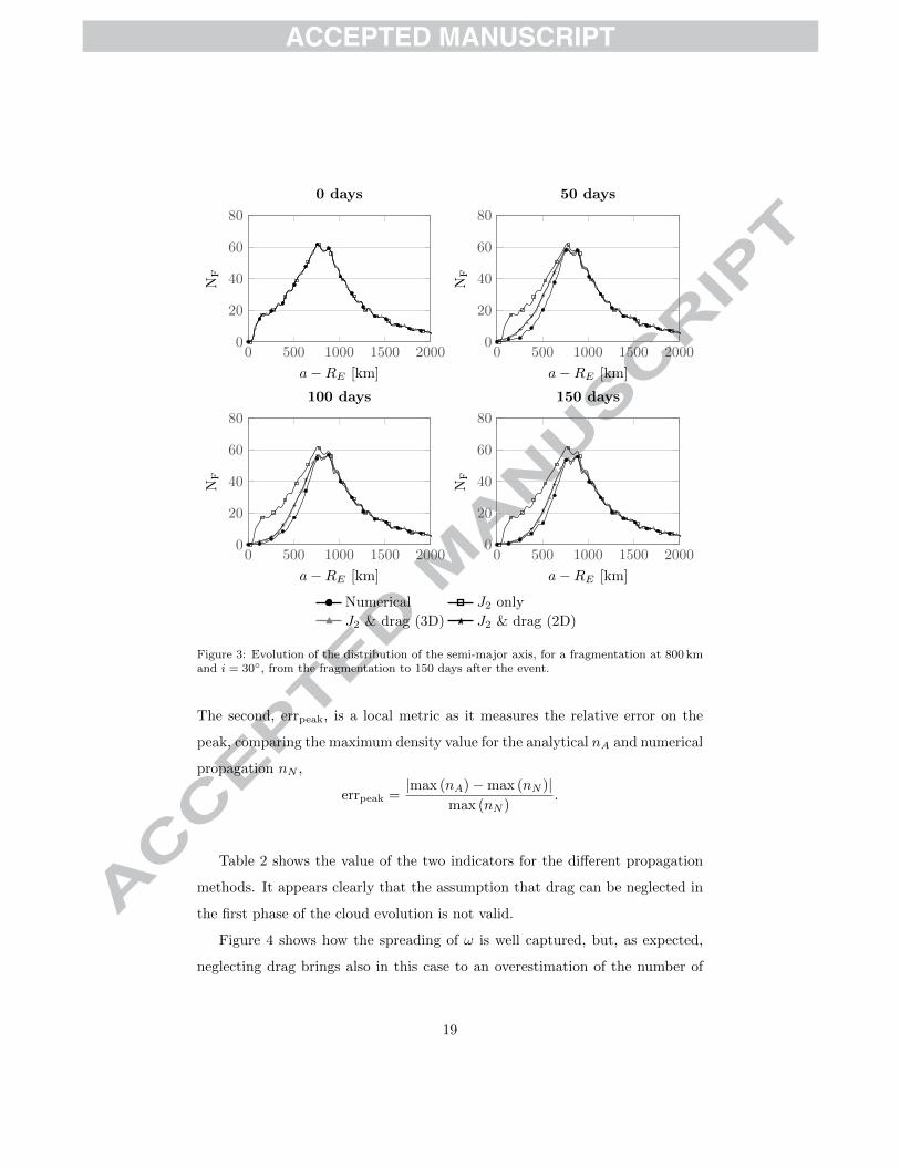
Figures 3, 4, 5 show respectively the evolution of the distributions in a,

ω, Ω for the proposed analytical methods and for the numerical propagation.

The accuracy in the description of the distribution in a is the most relevant

figure to consider as it has a direct impact on the estimated value of the spatial

density. From Figure 3 one can observe how neglecting the effect of drag leads

to an overestimation of the number of objects with low semi-major axis. Two

indicators are used to estimate the method accuracy. The first, errtot, is a metric

of the global accuracy of the method and measures the relative error of the total

number of fragments obtained by integrating the density curve in altitude (h)

errtot =|∫nA dh−

∫nN dh|∫

nN dh.

18

0 500 1000 1500 2000

0

20

40

60

80

a−RE [km]

NF

0 days

0 500 1000 1500 20000

20

40

60

80

a−RE [km]

NF

50 days

0 500 1000 1500 20000

20

40

60

80

a−RE [km]

NF

150 days

0 500 1000 1500 20000

20

40

60

80

a−RE [km]

NF

100 days

Numerical J2 only

J2 & drag (3D) J2 & drag (2D)

Figure 3: Evolution of the distribution of the semi-major axis, for a fragmentation at 800 kmand i = 30, from the fragmentation to 150 days after the event.

The second, errpeak, is a local metric as it measures the relative error on the

peak, comparing the maximum density value for the analytical nA and numerical

propagation nN ,

errpeak =|max (nA)−max (nN )|

max (nN ).

Table 2 shows the value of the two indicators for the different propagation

methods. It appears clearly that the assumption that drag can be neglected in

the first phase of the cloud evolution is not valid.

Figure 4 shows how the spreading of ω is well captured, but, as expected,

neglecting drag brings also in this case to an overestimation of the number of

19

−180 −90 0 90 1800

20

40

60

ω [deg]

NF

0 days

−180 −90 0 90 1800

20

40

60

ω [deg]

NF

50 days

−180 −90 0 90 1800

20

40

60

ω [deg]

NF

150 days

−180 −90 0 90 1800

20

40

60

ω [deg]

NF

100 days

Numerical J2 only

J2 & drag (3D) J2 & drag (2D)

Figure 4: Evolution of the distribution of the argument of the perigee, for a fragmentation at800 km and i = 30, from the fragmentation to 150 days after the event.

fragments. Figure 5 shows the evolution of the distribution of Ω. Observe

that in this case the initial condition was modified substituting the real initial

distribution where all fragments have Ω = 0 with a Gaussian distribution. This

was done to avoid numerical issues such as instabilities, even if some anomalous

peaks are still presents (e.g. the one at -5 degrees at t = 150 days).

In terms of computational time, all the analytical approaches are much faster

than the numerical propagation. The average running time over ten simula-

tions, as measured by Matlab built-in functions and for a PC with four CPUs

at 3.4GHz, is reported in Table 2; for the numerical propagation the average

20

−180 −90 0 90 1800

500

1000

1500

2000

Ω [deg]

NF

0 days

−180 −90 0 90 1800

20

40

60

80

100

Ω [deg]

NF

50 days

−180 −90 0 90 1800

10

20

30

40

Ω [deg]

NF

150 days

−180 −90 0 90 1800

10

20

30

40

Ω [deg]

NF

100 days

Numerical J2 only

J2 & drag (3D) J2 & drag (2D)

Figure 5: Evolution of the distribution of the longitude of the ascending node, for a fragmen-tation at 800 km and i = 30, from the fragmentation to 150 days after the event.

computational time is equal to 55 s2. Including drag doubles the computational

time , but the numbers are so low that there is not a practical convenience in

using the model with the Earth’s oblateness only. On the other hand, reducing

the number of parameters gives a larger speed-up while keeping a better level

of accuracy.

Given the performance both in terms of accuracy and computational time,

the application of the continuity equation to the initial phase of the cloud evolu-

tion appears promising. Future work will aim to use the analytical propagation

2The fact that the computational time is longer in this case than for the long term simu-lations studied in Section 6 is due to the fact that in the short time simulated here only a fewfragments decay.

21

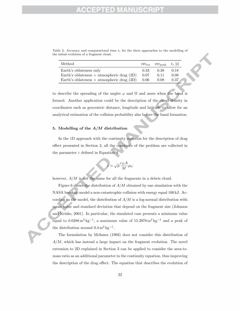
Table 2: Accuracy and computational time tc for the three approaches to the modelling ofthe initial evolution of a fragment cloud.

Method errtot errpeak tc [s]

Earth’s oblateness only 0.33 0.38 0.18Earth’s oblateness + atmospheric drag (2D) 0.07 0.11 0.08Earth’s oblateness + atmospheric drag (3D) 0.06 0.08 0.37

to describe the spreading of the angles ω and Ω and asses when the band is

formed. Another application could be the description of the cloud density in

coordinates such as geocentric distance, longitude and latitude to allow for an

analytical estimation of the collision probability also before the band formation.

5. Modelling of the A/M distribution

In the 1D approach with the continuity equation for the description of drag

effect presented in Section 2, all the constants of the problem are collected in

the parameter ε defined in Equation 4

ε =√µcDA

Mρ0;

however, A/M is not the same for all the fragments in a debris cloud.

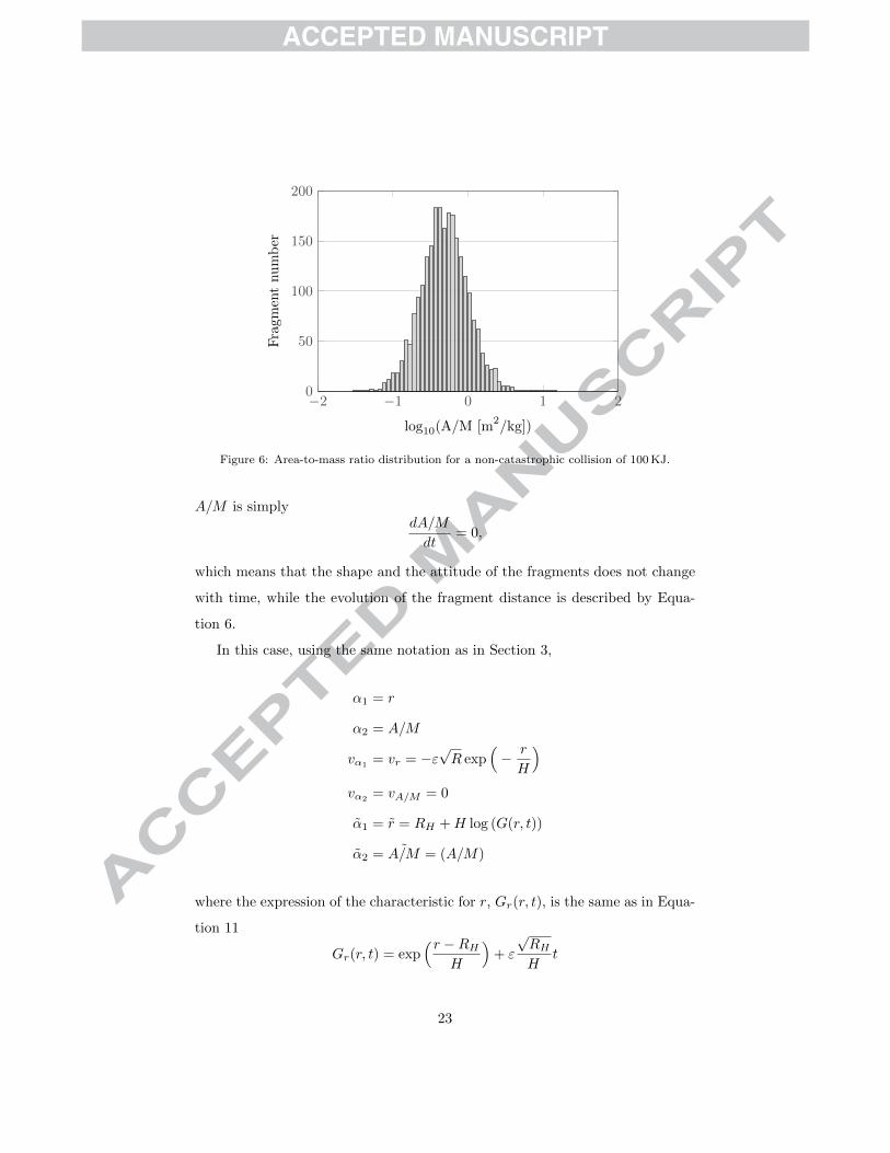
Figure 6 shows the distribution of A/M obtained by one simulation with the

NASA breakup model a non-catastrophic collision with energy equal 100 kJ. Ac-

cording to the model, the distribution of A/M is a log-normal distribution with

mean value and standard deviation that depend on the fragment size (Johnson

and Krisko, 2001). In particular, the simulated case presents a minimum value

equal to 0.0288 m2 kg−1, a maximum value of 15.3978 m2 kg−1 and a peak of

the distribution around 0.4 m2 kg−1.

The formulation by McInnes (1993) does not consider this distribution of

A/M , which has instead a large impact on the fragment evolution. The novel

extension to 2D explained in Section 3 can be applied to consider the area-to-

mass ratio as an additional parameter in the continuity equation, thus improving

the description of the drag effect. The equation that describes the evolution of

22

−2 −1 0 1 20

50

100

150

200

log10(A/M [m2/kg])

Fragm

entnumber

Figure 6: Area-to-mass ratio distribution for a non-catastrophic collision of 100 KJ.

A/M is simplydA/M

dt= 0,

which means that the shape and the attitude of the fragments does not change

with time, while the evolution of the fragment distance is described by Equa-

tion 6.

In this case, using the same notation as in Section 3,

α1 = r

α2 = A/M

vα1= vr = −ε

√R exp

(− r

H

)vα2 = vA/M = 0

α1 = r = RH +H log (G(r, t))

α2 = ˜A/M = (A/M)

where the expression of the characteristic for r, Gr(r, t), is the same as in Equa-

tion 11

Gr(r, t) = exp(r −RH

H

)+ ε

√RHH

t

23

0 500 1000 1500 2000

0

2

4

6

8

Altitude [km]

nx10

9[1/k

m3]

TB + 0 days

0 500 1000 1500 20000

2

4

6

8

Altitude [km]

nx10

9[1/k

m3]

TB + 333 days

0 500 1000 1500 20000

2

4

6

8

Altitude [km]

nx10

9[1/k

m3]

TB + 1000 days

0 500 1000 1500 20000

2

4

6

8

Altitude [km]

nx10

9[1/k

m3]

TB + 666 days

Numerical Analytical 1D (r)

Analytical 2D (a,A/M)

Figure 7: Evolution of the cloud density (n) profile as a function of time after the bandformation TB (TB = 95 days) for a fragmentation at 800 km, i = 0 degrees.

and vr depends on A/M through ε as shown in Equation 4. The final expression

for the fragment density, applying Equation 22, is

n(r,A/M, t) = n0(r,A/M)vr(r, A/M)

vr(r,A/M).

5.1. Results

Figure 7 compares the results of the analytical propagation with the output

of the numerical one. The results are expressed in terms of spatial density,

which in the case of the numerical propagation is obtained counting the number

of objects in spherical shells with thickness equal to 20 km. Figure 7 shows how

the 2D formulation is able to follow very well the evolution of the cloud and

24

represents a significant improvement of the 1D approach for treating A/M . In

particular, after 1000 days from the band formation, the relative error on the

peak errpeak is equal to 49% for the 1D method and 20% for the 2D one.

However, it has to be noted that treating A/M as an additional dimension

of the problem increases its complexity. In particular, here it is possible to

keep a 1D formulation of the problem and divide the fragments into Nb bins in

area-to-mass ratio, for example defining the bins in such a way that each one

contains the same number of fragments at the band formation (Letizia et al.,

2015a). For each bin, an average εj is assumed and the corresponding density

nj is obtained using Equation 12; all the partial densities nj are summed to

obtain the global cloud density n

n(r, t) =

Nb∑j

nj(r, t).

Figure 8 shows the density at 1000 days for a fragmentation at 800 km for

different formulations of the problem: both including 5 and 10 bins is possible

to obtain a result similar to the 2D approach around the peak area. Additional

analysis has shown that 10 is the optimal bins number in the trade-off between

computational time and relative error (Letizia et al., 2015a).

6. Modelling of the eccentricity distribution

The method explained in Section 2 is based on the hypothesis that the frag-

ments are on circular orbits: this allows obtaining a full analytical solution for

the spatial density evolution under the drag effect. However, this also limits

the applicability of the method to altitudes equal to and higher than 800 km.

In fact, at lower altitudes, even in case of a small value of eccentricity, the at-

mosphere density changes so largely along one single orbit that Equation 3 is

not accurate anymore Letizia et al. (2015a). For this reason, the eccentricity

should be included in the propagation. In particular, the problem is here formu-

lated in terms of the evolution of the debris cloud in the phase space defined by

25

0 500 1000 1500 20000

2

4

6

8

Altitude [km]

nx10

9[1/k

m3]

Numerical

Analytical (no bins)

Analytical (5 bins)

Analytical (10 bins)

Analytical (2D)

0 500 1000 1500 2000−1

−0.5

0

0.5

1

Altitude [km]

∆n/n

N

Figure 8: Density profile at 1000 days after the band formation TB (TB = 95 days) for afragmentation at 800 km, i = 0 degrees for different propagators and relative error measuredwith respect to the value obtained with the numerical propagation nN .

26

the semi-major a and the eccentricity e. In this case, the cloud spatial density

in [1/km3] is computed a posteriori through expressions such as the ones by

Kessler (1981) or Sykes (1990).

In order to apply the equations obtained in Section 3, an expression for the

rate of variation of a and e, respectively va and ve, is required. They both can

be obtained from the expression for the variation of the orbital parameters in

one orbit

∆a = −2πcDA

Ma2ρref exp

(− a−RH

H

)[I0 + 2eI1 +O(e2)

](35)

∆e = −2πcDA

Maρref exp

(− a−RH

H

)[I1 +

e

2(I0 + I2) +O(e2)

]; (36)

derived by King-Hele King-Hele (1987) for orbits whose eccentricity is between

0.01 and 0.1. It is assumed that the other orbital parameters are unchanged

under the hypothesis the Earth’s rotation is neglected.

In indicates the modified Bessel function of the first kind and order n with

argument z = ae/H, where H is the scale height coming from the exponential

model of the atmosphere; In(z) can be defined by the contour integral

In(z) =1

2πi

∮e(z/2)(t+1/t)t−n−1 dt; (37)

for n ∈ Z the definition can be simplified into

In(z) =1

π

∫ π

0

ez cos θ cosnθ dθ. (38)

The expression of the velocities is therefore

va = −√µacDAM

ρ0 exp(− a−RH

H

)f(a, e,H)

ve = −√µ

a

cDA

Mρ0 exp

(− a−RH

H

)g(a, e,H)

(39)

where

f(a, e,H) = I0 + 2eI1 +O(e2)

g(a, e,H) = I1 +e

2(I0 + I2) +O(e2).

(40)

27

Introducing the parameter ε as in Equation 4, the resulting system of equa-

tions is

dt

ds= 1

da

ds= −ε√a exp

(− a−RH

H

)f(a, e,H)

de

ds= − ε√

aexp

(− a−RH

H

)g(a, e,H)

dn

ds= −

[∂va∂a

+∂ve∂e

]n(a, e, t)

(41)

(42)

(43)

(44)

that, however, does not admit an analytical solution. Two approximations are,

therefore, introduced:√a ≈

√RH (45)

and

f(a, e,H) ≈ f(RH , e,H) g(a, e,H) ≈ g(RH , e,H); (46)

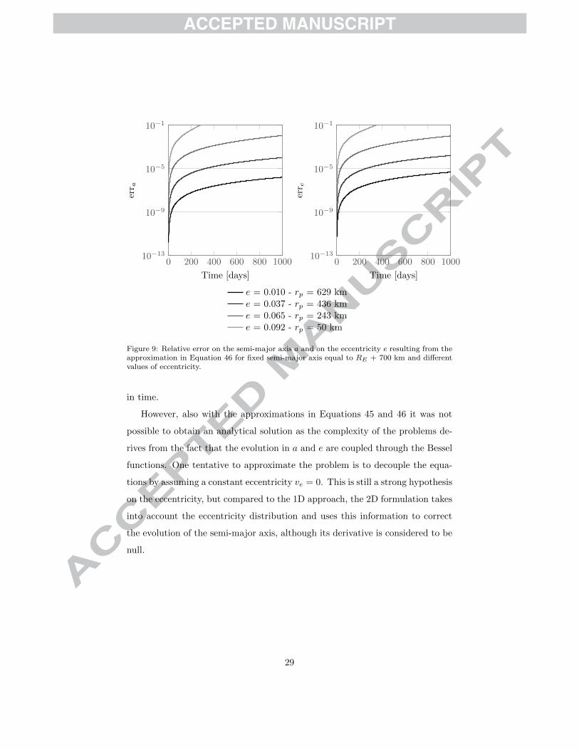
the impact of these approximations on the accuracy of the trajectory evolution

was verified and considered acceptable, as shown in Figure 9. It shows the

relative error on the semi-major axis erra and on the eccentricity erre

erra =a− aNaN

erre =e− eNeN

where (a, e) are the values of the orbital parameters obtained introducing the

approximations in Equations 45 and 46, and (aN , eN ) are the values obtained

from the numerical propagation, without any approximation. In all cases shown

in Figure 9, the semi-major axis is set equal to RE + 700 km while four different

values of eccentricity are considered. The error is very low for the first two case

(e = 0.010 and e = 0.037), whose curves lay on the x-axis in Figure 9. In

general, the error is lower than 1% both for the semi-major axis and for the

eccentricity for all the cases except the one with e = 0.092, whose perigee is

equal to 50 km, the threshold value below which the fragments are considered

to being re-entering. These fragments are likely to re-enter much faster than

the other ones, so also their impact on the propagation of the cloud is limited

28

0 200 400 600 800 100010−13

10−9

10−5

10−1

Time [days]

err a

0 200 400 600 800 100010−13

10−9

10−5

10−1

Time [days]

err e

e = 0.010 - rp = 629 kme = 0.037 - rp = 436 kme = 0.065 - rp = 243 kme = 0.092 - rp = 50 km

Figure 9: Relative error on the semi-major axis a and on the eccentricity e resulting from theapproximation in Equation 46 for fixed semi-major axis equal to RE + 700 km and differentvalues of eccentricity.

in time.

However, also with the approximations in Equations 45 and 46 it was not

possible to obtain an analytical solution as the complexity of the problems de-

rives from the fact that the evolution in a and e are coupled through the Bessel

functions. One tentative to approximate the problem is to decouple the equa-

tions by assuming a constant eccentricity ve = 0. This is still a strong hypothesis

on the eccentricity, but compared to the 1D approach, the 2D formulation takes

into account the eccentricity distribution and uses this information to correct

the evolution of the semi-major axis, although its derivative is considered to be

null.

29

0 1000 2000 3000 40000

0.1

0.2

0.3

0.4

a−RE [km]

e[-]

Figure 10: Distribution of semi-major axis and eccentricity, for a fragmentation at 700 km, atthe band formation (92 days after the fragmentation).

Therefore, the problem is solved setting

α1 = a (47)

α2 = e (48)

vα1= va = −

õRH

cDA

Mρ0 exp

(− a−RH

H

)f(RH , e(a), H) (49)

vα2= ve = 0 (50)

α1 = a = H log[(exp

(a−RHH

)+ εf(RH , e(a), H)

√RHH

t]

(51)

α2 = e = e. (52)

Note that an heuristic was adopted in Equation 49, introducing e(a) that

expresses a reference value of the eccentricity for each value of the semi-major

axis. This means that, given a value of the semi-major axis aj , e(aj) is the con-

stant value associated with it. The value of e(a) can be obtained starting from

the initial distribution n0(a, e): the function e0 is built assigning to each value

of the semi-major axis the value of eccentricity where the density is maximum;

30

for example, for a = aj

e(aj) = ej : nj = n0(aj , ej) = max (n0(aj , e)).

The resulting function for the case at 700 km is shown in Figure 10.

6.1. Results

The result of the numerical propagation in terms of density in the phase

space is shown in Figure 11a: the domain is divided into cells with width equal

to 25 km in semi-major axis and 0.005 in eccentricity; the plot shows the number

of fragments NF in each cell. The plot on the left refers to the moment of band

formation and it is easy to recognise the v-shaped distribution of eccentricity

with semi-major axis, which is an alternative representation of the well known

Gabbard diagram (Portree and Loftus, 1999). The v-shaped curve is centred

on the altitude of the parent orbit: the leg on the left represents the fragments

whose orbits have the fragmentation location as apogee, the leg on the right

those with the fragmentation location as perigee. The plot on the right refers

instead to the cloud density at 1000 days after the band formation: the number

of fragments is reduced and the fragments with low semi-major axis are on

circular orbits, therefore one leg of the v-shaped distribution disappears.

The same plots can be obtained also with the analytical approach in 2D

(Figure 11b) which provides a distribution of fragments extremely similar to

the numerical simulation. The most evident difference in the density after 1000

days from the band formation is that the analytical approach underestimates

the number of fragments with e ≈ 0.

This fact is even clearer from Figure 12 that shows the distributions of

semi-major axis and eccentricity for the numerical propagation and for the 2D

analytical approach at the different time instants. After 1000 days from the

band formation, the distribution of the semi-major axis is well captured (Figure

12); on the other hand, the analytical approach is not able to represent the peak

at e ≈ 0 in the eccentricity distribution. This happens because the analytical

31

0 500 1000 1500 20000

0.05

0.1

0.15

0.2

a−RE [km]

eTB + 0 days

0 500 1000 1500 20000

0.05

0.1

0.15

0.2

a−RE [km]

e

TB + 1000 days

0

10

20

30

NF

(a) Numerical propagation

0 500 1000 1500 20000

0.05

0.1

0.15

0.2

a−RE [km]

e

TB + 0 days

0 500 1000 1500 20000

0.05

0.1

0.15

0.2

a−RE [km]

e

TB + 1000 days

0

10

20

30

NF

(b) Analytical propagation

Figure 11: Visualisation of cloud density (in number of fragments) at the band formation(TB = 92 days) and after 1000 days for two propagation methods.

32

0 500 1000 1500 2000

0

20

40

60

80

100

a−RE [km]

NF

TB + 0 days

0 500 1000 1500 20000

20

40

60

80

100

a−RE [km]

NF

TB + 1000 days

0 0.1 0.2 0.30

50

100

150

e [-]

NF

Numerical

Analytical 2D (a, e)

0 0.1 0.2 0.30

50

100

150

e [-]

NF

Figure 12: Distribution of semi-major axis and eccentricity, for a fragmentation at 700 km, atthe band formation (TB = 92 days) and after 1000 days.

propagation is obtained starting from the equation

de

dt= 0

so the progressive reduction of eccentricity is lost.

Despite this error, it is possible to see from Figure 13 how the 2D approach

represents in any case a remarkable improvement compared to the 1D method

used in Letizia et al. (2015a). Figure 13 shows the cloud density profile after

1000 days from the band formation for a fragmentation at six different altitudes.

The value of spatial density for the numerical propagation is obtained dividing

the altitude in bin with width equal to 25 km, counting the number of fragments

in each bin and dividing by the volume of the corresponding spherical shell. For

the numerical propagation ten runs of the breakup model were performed to

take into account the random parameters within the model.

33

0 500 1000 1500 20000

0.5

1

1.5

2

Altitude [km]

n×10

9[1/k

m3]

81 fragments

Numerical

Analytical 1D (r)

Analytical 2D (a, e)

(a) Perigee altitude: 500 km

0 500 1000 1500 20000

0.5

1

1.5

2

Altitude [km]

n×10

9[1/k

m3]

457 fragments

(b) Perigee altitude: 600 km

0 500 1000 1500 20000

2

4

6

Altitude [km]

n×

109[1/k

m3]

961 fragments

(c) Perigee altitude: 700 km

0 500 1000 1500 20000

2

4

6

Altitude [km]

n×

109[1/k

m3]

1373 fragments

(d) Perigee altitude: 800 km

0 500 1000 1500 20000

2

4

6

8

Altitude [km]

n×

109[1/k

m3]

1722 fragments

(e) Perigee altitude: 900 km

0 500 1000 1500 20000

2

4

6

8

Altitude [km]

n×

109[1/k

m3]

2009 fragments

(f) Perigee altitude: 1000 km

Figure 13: Cloud density after 1000 days from the band formation for six different collisionaltitudes.

34

At high altitudes the accuracy of the 1D and the 2D formulation is similar.

At 700 km only the 2D method is able to identify the correct peak location and

the relative error on the peak height is halved. The case of a fragmentation

at 600 km shows that even the 2D approach is not able to obtain an accurate

prediction of the cloud evolution at such low altitudes. Note, however, that if

the fragmentation happens at very low altitude, the number of fragments after

1000 days is very low, so even the use of a continuum approach is questionable

for such a limited number of samples.

The relative error on density peak and on the total number of fragments for

the methods is plotted in Figure 14. Setting a threshold value at 20%, which

corresponds to a good visual agreement between the density profile obtained

with the numerical propagation and the one with the analytical one, the 1D

approach is applicable above 800 km and the 2D approach instead can be applied

from 700 km and the average error on the respective ranges of applicability is

similar. This extends the applicability of the method in a such a way that it can

be applied along the whole altitude range of the sun-synchronous orbits, where

the debris density is the highest and where there are many critical objects in

terms of possible future fragmentations.

The improvement in the results is associated with a small increase in the

computational time that can be evaluated from Figure 15, which shows the

time required to estimate the cloud density 1000 days after the band formation.

The measured computational times refer to a PC with 4 CPUs at 3.40 GHz and

the numbers in Figure 15 refer to the average over ten runs. All the codes are

written in Matlab and parallelised. The propagation with the 2D formulation

requires more than double the time of the 1D (1.34 s compared to 0.66 s), but

the computational time is still lower than the numerical propagation. The final

step of conversion from the density in the (a, e)-plane into the spatial density in

1/km3 appears quite expensive (2.17 s). One can observe that for applications

when the propagation method is used to compute the collision probability for

a spacecraft crossing the cloud the value of n is required only at the target

altitude, so the computation is faster. On the other hand, when the cloud

35

600 800 100010−2

10−1

100

Altitude [km]

err p

eak

600 800 100010−2

10−1

100

Altitude [km]

err t

ot

1D (r)

2D (a, e)

Figure 14: Accuracy of the method, measured by the relative error on peak and total fragmentnumber after 1000 days from the band formation, as a function of the fragmentation altitude,for analysed propagation techniques.

0 5 10 15 20 25 30

1D

2D

Numerical

Computational time [s]

Breakup Initial prop.

Bins def. Fitting

Final prop. Density

Figure 15: Computational time for a PC with 8 CPUs at 3.40 GHz and the division of thecloud into ten bins in A/M .

36

propagation is used for such application, it is not sufficient to know the state of

the cloud at the final time, but a fine time step should be adopted. As at each

time step the fit of a 2D function is performed, the operation could be expensive,

so future work will investigate alternative implementations. In any case, it is

important to highlight that the running time is only a part of the computational

effort required by a simulation. The main advantage of the proposed approach

is that describing the problem in terms of spatial density instead of studying

the position of each objects reduces the required RAM. This means that large

fragmentations (e.g. with more than 10000 fragments) can me simulated on

normal PCs, without the used of supercomputers.

The saving in the computational time achieved also with the 2D approach

suggests that it also can be applied to study many different fragmentation sce-

narios to understand which conditions affect the most the debris environment

and the collision probability for operational spacecraft.

7. Conclusions

Studies on space debris usually refer only to the population of objects larger

than 10 cm. Large objects are, indeed, the most dangerous as, in case of col-

lision, they are able to destroy a satellite and to create larger debris cloud.

However, also small debris fragments can represent a relevant hazard to opera-

tional satellites, but their contribution to the collision risk is often disregarded

for two main reasons: the lack of a catalogue with data on single small objects

and the requirement for a different approach to propagate them. In fact, the

number of small fragments is so large that the traditional propagation of all

objects is not feasible because it would result into a prohibitive computational

effort.

Some models dealt with this issue defining some representative objects that

are studied instead of the actual population of small fragments. This work pro-

poses instead a continuous approach based on the description of the fragments

dynamics in terms of the evolution of their spatial density. The method was

37

already applied to describe the evolution of debris clouds under the effect of

drag for orbits at minimum 800 km. The long term evolution of the cloud is ob-

tained by applying the continuity equation that, introducing some hypotheses,

admits an analytical solution. The possibility of writing an explicit expression

for the density, as a function of time and distance, provides a very quick way

to describe the small fragments dynamics and their contribution to the collision

probability.

Here the method applicability was extended by switching to a 2D formulation

where the coordinates are the most relevant parameters of the studied scenario.

In this way it was possible to apply the density method to describe also the effect

of the Earth’s oblateness and the distribution of the area-to-mass ratio and of the

eccentricity among the fragments. This last application, in particular, extends

the method applicability down to 700 km, so that it can be used to describe the

evolution of the fragment clouds originating from all the regions with the highest

space debris density, such as sun-synchronous orbits. On the other hand, the

possibility of modelling also the effect of the Earth’s oblateness suggests that it

should be possible to formulate an analytical approach able to follow the debris

clouds both in short and in long time-scales.

Acknowledgement

Francesca Letizia is supported by the Amelia Earhart Fellowship for the

academic year 2013/2014. Camilla Colombo acknowledges the support received

by the Marie Curie grant 302270 (SpaceDebECM - Space Debris Evolution,

Collision risk, and Mitigation), within the 7th European Community Framework

Programme.

References

Ashenberg, J., 1994. Formulas for the phase characteristics in the problem of

low-Earth-orbital debris. Journal of Spacecraft and Rockets 31, 1044–1049.

doi:10.2514/3.26556.

38

Ashenberg, J., Broucke, R., 1993. The effect of the Earth’s oblateness on the

long-term dispersion of debris. Advances in Space Research 13, 171–174.

Colombo, C., 2015. Long-term evolution of highly-elliptical orbits: Luni-solar

perturbation effects for stability and re-entry, in: 25th AAS/AIAA Space

Flight Mechanics Meeting. AAS-15-395.

Colombo, C., McInnes, C.R., 2011. Evolution of swarms of smart dust space-

craft, in: New Trends in Astrodynamics and Applications VI, Courant Insti-

tute of Mathematical Sciences, New York.

Evans, L., 1998. Partial Differential Equations. Graduate studies in mathemat-

ics, American Mathematical Society.

Gor’kavyi, N., 1997. A new approach to dynamical evolution of interplanetary

dust. The Astrophysical Journal 474, 496–502. doi:10.1086/303440.

Gor’kavyi, N., Ozernoy, L., Mather, J., Taidakova, T., 1997. Quasi-stationary

states of dust flows under Poynting-Robertson drag: New analytical and nu-

merical solutions. The Astrophysical Journal 488, 268–276.

Hoots, F.R., Hansen, B.W., 2014. Satellite breakup debris cloud characteriza-

tion, in: 24th AAS/AIAA Space Flight Mechanics Meeting, Santa Fe. AAS

14-329.

IADC Steering Committee, 2013. IADC Assessment Report for 2011. Technical

Report IADC-12-06. Inter-Agency Space Debris Coordination Committee.

Izzo, D., 2002. Statistical modelling of orbits and its application to trackable

objects and to debris clouds. Ph.D. thesis. Universita La Sapienza.

Jehn, R., 1991. Dispersion of debris clouds from In-orbit fragmentation events.

ESA Journal 15, 63–77.

Johnson, N.L., Krisko, P.H., 2001. NASA’s new breakup model of EVOLVE 4.0.

Advances in Space Research 28, 1377–1384. doi:10.1016/S0273-1177(01)

00423-9.

39

Kessler, D.J., 1981. Derivation of the collision probability between

orbiting objects: the lifetimes of jupiter’s outer moons. Icarus

48, 39–48. URL: http://linkinghub.elsevier.com/retrieve/pii/

0019103581901512, doi:10.1016/0019-1035(81)90151-2.

King-Hele, D., 1987. Satellite orbits in an atmosphere: theory and application.

Blackie, Glasgow and London.

Krisko, P.H., 2011. Proper Implementation of the 1998 NASA Breakup Model.

Orbital Debris Quarterly News 15, 1–10.

Letizia, F., Colombo, C., Lewis, H.G., 2015a. Analytical model for the propaga-

tion of small debris objects clouds after fragmentations. Journal of Guidance,

Control, and Dynamics 38, 1478–1491. doi:10.2514/1.G000695.

Letizia, F., Colombo, C., Lewis, H.G., 2015b. Collision probability due to space

debris clouds through a continuum approach. Journal of Guidance, Control,

and Dynamics URL: http://arc.aiaa.org/doi/abs/10.2514/1.G001382,

doi:10.2514/1.G001382. accessed on September 10, 2015.

McInnes, C.R., 1993. An analytical model for the catastrophic production of

orbital debris. ESA Journal 17, 293–305.

McInnes, C.R., 1994. Compact analytic solutions for a decaying, precessing

circular orbit. The Aeronautical Journal 98, 357–360.

McInnes, C.R., 2000. Simple analytic model of the long term evolution of

nanosatellite constellations. Journal of Guidance Control and Dynamics 23,

332–338. doi:10.2514/2.4527.

McKnight, D.S., 1990. A phased approach to collision hazard analysis. Advances

in Space Research 10, 385–388. doi:10.1016/0273-1177(90)90374-9.

McKnight, D.S., Di Pentino, F.R., Knowles, S., 2014. Massive collisions in LEO

– A catalyst to initiate ADR, in: 65th International Astronautical Congress,

Toronto. IAC-14-A.6.2.1.

40

Nazarenko, A., 1997. The development of the statistical theory of a satellite

ensemble motion and its application to space debris modeling, in: Second

European Conference on Space Debris. URL: http://adsabs.harvard.edu/

full/1997ESASP.393..233N.

Nazarenko, A., 2002. Modeling Technogenous Contamination of the Near-

Earth Space. Solar System Research 36, 513–521. URL: http://

link.springer.com/article/10.1023/A%3A1022113421686, doi:10.1023/

A:1022113421686.

Portree, D.S.F., Loftus, J.P., 1999. Orbital Debris: A Chronology. Technical

Report NASA/TP-1999-208856. NASA.

Rossi, A., Anselmo, L., Cordelli, A., Farinella, P., Pardini, C., 1998. Modelling

the evolution of the space debris population. Planetary and Space Science 46,

1583–1596. doi:10.1016/S0032-0633(98)00070-1.

Smirnov, N., Nazarenko, A., Kiselev, A., 2001. Modelling of the space debris

evolution based on continua mechanics, in: Third European Conference on

Space Debris. URL: http://adsabs.harvard.edu/full/2001ESASP.473.

.391S.

Sykes, M., 1990. Zodiacal dust bands: Their relation to asteroid families.

Icarus 9. URL: http://www.sciencedirect.com/science/article/pii/

001910359090117R.

Valk, S., Lemaıtre, A., Deleflie, F., 2009. Semi-analytical theory of mean orbital

motion for geosynchronous space debris under gravitational influence. Ad-

vances in Space Research 43, 1070–1082. doi:10.1016/j.asr.2008.12.015.

Vallado, D.A., 2013. Fundamentals of astrodynamics and applications. 4th ed.,

Springer. Pages 551–573, 619–688. ISBN: 978-1881883180.

White, A.E., Lewis, H.G., 2014. The many futures of active debris removal.

Acta Astronautica 95, 189–197. doi:10.1016/j.actaastro.2013.11.009.

41

Xu, Y.L., Horstman, M., Krisko, P., Liou, J.C., Matney, M., Stansbery, E.,

Stokely, C., Whitlock, D., 2009. Modeling of LEO orbital debris populations

for ORDEM2008. Advances in Space Research 43, 769 – 782. doi:http:

//dx.doi.org/10.1016/j.asr.2008.11.023.

42