Continuity equation and characteristic flow for scalar ...
63
HAL Id: hal-02594303 https://hal.archives-ouvertes.fr/hal-02594303v3 Submitted on 19 Apr 2021 HAL is a multi-disciplinary open access archive for the deposit and dissemination of sci- entific research documents, whether they are pub- lished or not. The documents may come from teaching and research institutions in France or abroad, or from public or private research centers. L’archive ouverte pluridisciplinaire HAL, est destinée au dépôt et à la diffusion de documents scientifiques de niveau recherche, publiés ou non, émanant des établissements d’enseignement et de recherche français ou étrangers, des laboratoires publics ou privés. Continuity equation and characteristic flow for scalar Hencky plasticity Jean-François Babadjian, Gilles A. Francfort To cite this version: Jean-François Babadjian, Gilles A. Francfort. Continuity equation and characteristic flow for scalar Hencky plasticity. Communications on Pure and Applied Mathematics, Wiley, 2021. hal-02594303v3
Transcript of Continuity equation and characteristic flow for scalar ...

HAL Id: hal-02594303https://hal.archives-ouvertes.fr/hal-02594303v3
Submitted on 19 Apr 2021
HAL is a multi-disciplinary open accessarchive for the deposit and dissemination of sci-entific research documents, whether they are pub-lished or not. The documents may come fromteaching and research institutions in France orabroad, or from public or private research centers.
L’archive ouverte pluridisciplinaire HAL, estdestinée au dépôt et à la diffusion de documentsscientifiques de niveau recherche, publiés ou non,émanant des établissements d’enseignement et derecherche français ou étrangers, des laboratoirespublics ou privés.
Continuity equation and characteristic flow for scalarHencky plasticity
Jean-François Babadjian, Gilles A. Francfort
To cite this version:Jean-François Babadjian, Gilles A. Francfort. Continuity equation and characteristic flow for scalarHencky plasticity. Communications on Pure and Applied Mathematics, Wiley, 2021. hal-02594303v3
Continuity equation and characteristic flow for scalarHencky plasticity
JEAN-FRANÇOIS BABADJIANUniversité Paris-Saclay
AND
GILLES A. FRANCFORTUniversité Paris-Nord & Courant Institute
Abstract
We investigate uniqueness issues for a continuity equation arising out of the simplest modelfor plasticity, Hencky plasticity. The associated system is of the form curl (µσ) = 0 whereµ is a nonnegative measure and σ a two-dimensional divergence free unit vector field.After establishing the Sobolev regularity of that field, we provide a precise description ofall possible geometries of the characteristic flow, as well as of the associated solutions.
1. Introduction 12. Notation and preliminaries 113. Hencky plasticity 134. Sobolev regularity of the stress 145. Rigidity properties of the solutions 236. Geometry of the solutions 34Appendix. 58Bibliography 61
1 Introduction
1.1 The mathematical subtextIt is by now well established that the solutions µ of the continuity equation
div(µb) = 0,
for some given vector field b : RN → RN , are closely related to the notion of char-acteristics, that is to the solutions X of the ordinary differential equation
dXds
(s) = b(X(s)), s ≥ 0,
X(0) = x.

2 J.-F. BABADJIAN, G.A. FRANCFORT
When b is a Lipschitz continuous vector field, the Cauchy-Lipschitz theorem forODE’s provides a complete picture of the solutions. For less regular b’s, the theoryof regular Lagrangian flows initiated by R. DiPerna and P.-L. Lions [21] and pur-sued notably in [1, 15] has had tremendous success in handling such problems inthe context of Hamiltonian flows, i.e., under the additional assumption that divb iswell controlled, e.g. in L∞(RN).
We propose to investigate a closely related question in a two-dimensional set-ting where b = σ⊥ is the π/2-rotation of some σ ∈ L∞(R2;R2)∩H1
loc(R2;R2). Inthat setting, the continuity equation takes the form
(1.1) curl (µσ) = 0 ⇐⇒ div(µσ⊥) = 0.
The field σ under consideration in (1.1) is a divergence free field such that divσ⊥ =−curl σ only belongs to L2
loc(R2). As a consequence we do not control the so-called compressibility constant. The available theoretical tools developed in [21,1, 15] cannot produce the kind of uniqueness obtained in e.g. [15, Corollary 2.10].Note that here the ODE defining the characteristic flow follows a gradient flowstructure, rather than that of a Hamiltonian flow.
As will be discussed in Subsection 1.2, the existence of a nonnegative mea-sure µ which solves (1.1) (in a sense that will be specified in Section 3) is se-cured. However we have no information about uniqueness. The problem wewill detail in Subsection 1.2 and Section 3 exhibits additional structure. First itlives in a bounded domain Ω of R2 and the divergence free field σ belongs toL∞(Ω;R2)∩ H1
loc(Ω;R2). Further, µ is a nonnegative bounded Radon measuresupported on Ω and µσ is well-defined as a bounded Radon measure supported onΩ. Consequently, there is u ∈ BV (Ω) such that Du = µσ . That function is furtherassigned a prescribed exterior trace w on ∂Ω. Finally, it might be so that |σ | ≡ 1on an open subdomain of Ω; see the example discussed in Subsection 1.2. Thismotivates our choice of studying (1.1) under the following assumptions:
(1.2)
σ ∈ H1
loc(Ω;R2),
|σ |= 1 a.e. in Ωp open convex subset of Ω,
divσ = 0 in Ω.
From the standpoint of σ the setting is a particular case of that expounded uponin [30]. The additional information here is that σ ∈ H1
loc(Ω;R2) and it allows usto provide a very detailed description of the characteristics which, restricted toΩp, are straight lines in the direction of σ⊥ (a constant field along those lines) inSection 6.
But even an intimate knowledge of the characteristics does not yield any unique-ness result for the solution µ to the continuity equation (1.1). In our setting weprove in Section 5.2 that the associated function u remains constant along the char-acteristic lines as suggested by the formal computationdds
u(x+ sσ⊥(x))=Du(x+ sσ
⊥(x)) ·σ⊥(x)=Du(x+ sσ⊥(x)) ·σ⊥(x+ sσ
⊥(x))=0

CONTINUITY EQUATION IN HENCKY PLASTICITY 3
since Du = µσ . This also is not sufficient to claim uniqueness of the solution µ
to the continuity equation, most notably because, as explained in Remark 6.24, Ωpcannot coincide with Ω so that we do not know how to relate the values of u on Ωpto the boundary values of u, this independently of whether or not the internal traceof u on ∂Ω coincides with the given external trace w.
The full results are given in Theorem 1.3. They are expressed in a slightlydifferent language, that of plasticity because, as will become clear in the next sub-section, our main motivation derives from issues of uniqueness of the plastic strainin Von Mises plasticity. The connection with hyperbolicity à la (1.1) is uncoveredin Subsection 1.2.
1.2 The specific contextWhen departing from a completely reversible behavior, fluid mechanics essen-
tially follows a unique path, that of viscosity. In its simplest manifestation, Eulerequations cede the ground to Navier-Stokes equations which become the templatefor classical fluid behavior. Even non-Newtonian fluids usually exhibit viscosity,although one that may depend on a variety of kinematic or internal variables. Whenit comes to solids, while elasticity is the universally adopted reversible behavior,the irreversibility palette is much richer. This is so because solid mechanics en-codes geometry and not only flow. As for fluids, viscosity is one expression ofdissipation, leading to various kinds of viscoelastic models which, by the way,are mathematically much easier to handle in the case of solids. But many otherkinds of dissipative behaviors may occur, together with, or separate from viscosity.Their essential distinguishing feature is rate-independence: Material response is,up to rescaling, impervious to the loading rate. In that class, the best-establishedbehavior is plasticity, and, within plasticity, Von Mises plasticity. While other rate-independent behaviors are still a modeling challenge, Von Mises plasticity can bethought of as the solid equivalent to Navier-Stokes, that is an admittedly simplisticmodel that however contains key ingredients for explaining much of the underlyingphysics at the macroscopic level.
Of course, because of geometry, this assertion should be nuanced: Von Misesplasticity is a perfectly sound model as long as deformations are small, that isas long as the kinematics of the deformation does not result in large changes ofshape. Models for large deformations are not completely settled at present, evenin the absence of irreversibility. In spite of major advances in the past 40 yearsspearheaded by the work of J.M. Ball [10], finite elasticity is far from a completetheory, while finite plasticity is a minefield.
Von Mises plasticity, also called Prandtl-Reuss elasto-plasticity with a VonMises yield criterion, consists in a system of time dependent equations below.There, we denote by Ω the three-dimensional domain under consideration and, forsimplicity, place ourselves in a quasi-static setting, that is in the absence of inertia.We further assume homogeneity and take all material parameters to be identically1 (with the right units).

4 J.-F. BABADJIAN, G.A. FRANCFORT
The displacement field u(t) : Ω→R3 is constrained by a time-dependent Dirich-let boundary condition u(t) = w(t) on ∂Ωd , a relatively open subset of ∂Ω, whichconstitutes the Dirichlet part of the boundary. The associated linearized strainEu(t) := 1
2(∇u(t)+∇u(t)T ) is additively decomposed into the elastic strain e(t)(a 3×3 symmetric matrix) and the plastic strain p(t) (a trace-free 3×3 symmetricmatrix), i.e.,
Eu(t) = e(t)+ p(t), with tr(p(t)) = 0.
We assume, for simplicity, that the only driving mechanism, besides the im-posed displacement w(t), is a surface load g(t); there are no body loads. With ourassumptions, the Cauchy stress σ(t), is simply
σ(t) = e(t).
It is in quasi-static equilibrium, i.e.,
divσ(t) = 0 in Ω, σ(t)ν = g(t) on ∂Ωn := ∂Ω\∂Ωd
(ν is the outer normal to ∂Ωn), while its deviatoric part σD(t) :=σ(t)− 13 tr(σ(t))Id
satisfies the Von Mises yield criterion,
|σD(t,x)| ≤√
23
at every point x ∈ Ω.
The deviatoric stress σD(t) and the plastic strain rate p(t) are related, at everypoint x ∈ Ω, through the so-called flow rule
(1.3) p(t,x) = λ (t,x)σD(t,x), with
λ (t,x)≥ 0,
λ (t,x) = 0 if |σD(t,x)|<√
23 .
In other words, whenever the (deviatoric part of the) stress reaches the boundary ofits admissible set, the plastic strain should flow in the direction normal to that set.
The modern mathematical treatment of Von Mises plasticity finds its roots inthe work of P.-M. Suquet [37], later completed by various works (see e.g. [38, 31,4, 5, 6]). That work was revisited some 20 years later by G. Dal Maso, A. De Si-mone and M. G. Mora [16] within the framework of the variational theory of rateindependent evolutions popularized by A. Mielke (see e.g. [33]). The basic tenetthere is that the evolution can be viewed as a time-parameterized set of minimiza-tion problems for the sum of the elastic energy and of the add-dissipation. Theminimizers should also be such that an energy conservation statement, amountingto a kind of Clausius-Duhem inequality, is satisfied throughout the evolution.
In any case, for a Lipschitz bounded domain Ω and smooth enough w and g (seee.g. [24, Remark 2.10]), the resulting evolutions t 7→ (u(t),e(t), p(t)) are found tolive in AC([0,T ];BD(Ω)× L2(Ω;R6)×M (Ω∪ ∂Ωd ;R6)). Here, BD(Ω) standsfor the space of functions of bounded deformation, i.e., integrable vector fieldsv : Ω → R3 whose distributional symmetrized gradient Ev = 1
2(Dv + DvT ) is abounded measure in Ω and M (Ω∪ ∂Ωd ;R6) stands for the space of R6-valued

CONTINUITY EQUATION IN HENCKY PLASTICITY 5
bounded Radon measures on Ω∪ ∂Ωd (see [24] under those conditions). Further,uniqueness of e(t), hence of σ(t) is guaranteed. Such however is not the case forp(t), hence for u(t). The first example of non-uniqueness was presented in [37,Section 2.1] while [19, Section 10] introduces the first examples of uniqueness. Inthose references the setting is essentially 1D. To our knowledge, the only examplesof determination of uniqueness or non-uniqueness in 3D can be found in [26, 27].There, the discussion around uniqueness is centered around the equation that theLagrange multiplier λ in (1.3) must satisfy when |σD(t,x)|=
√2/3.
We next formally manipulate the equations at a given fixed time t. Indeed,since p = Eu− e, or still λσD = Eu− σ , we can use the compatibility equationsfor symmetrized gradient, that is, for all 1 ≤ i, j,k, l ≤ 3,
∂ 2(Eu)i j
∂xk∂xl+
∂ 2(Eu)kl
∂xi∂x j− ∂ 2(Eu)ik
∂x j∂xl− ∂ 2(Eu)il
∂x j∂xk= 0.
We obtain a system of 6 equations, namely,
(1.4) (σD)i j∂ 2λ
∂xk∂xl+(σD)kl
∂ 2λ
∂xi∂x j− (σD)ik
∂ 2λ
∂x j∂xl− (σD)il
∂ 2λ
∂x j∂xk
(+ terms of lower order in λ ) =−(curl curl (σ))i jkl.
In the example investigated in [26], the stress field σ is constant, so that the lowerorder terms disappear as well as the right-hand side, and the formal manipulationscan be justified. We then have to deal with a bona fide system of second orderlinear partial differential equations for the measure λ of the form
D∇2λ (t) = 0,
with D a constant 6×6 matrix. Whenever the determinant of D is not 0, ∇2λ (t)≡0; then, because of the specific setting in that example, λ (t) is x-independent, fromwhich it follows that p(t) is an x-independent plastic strain p(t). With that result athand, p(t) is easily shown to be unique; the example in [27], while more intricate,goes along the same lines. Otherwise, the system reduces to a spatial hyperbolicequation for λ (t) and then uniqueness depends on whether the associated charac-teristics coming out of ∂Ωd fill the whole domain. Roughly speaking, if they do,then uniqueness is obtained. If they don’t, then non-uniqueness can be drastic be-cause plastic strains that are as badly behaved as one desires (for example plasticstrains supported on Cantor sets) can appear at any time t in the region not reachedby those characteristics. So one could then impose a large enough homogeneousboundary condition and the stress field would consequently be constant while apossible plastic strain would be spatially homogeneous. Yet, arbitrary localizednon-zero plastic strains could be superimposed at any later time. This is remi-niscent of what was recently observed by C. De Lellis and L. Székelyhidi whendealing with non-uniqueness in Euler equations (see [18] and subsequent works),with the important caveat that plastic strains, once turned on, cannot be turned offbecause of dissipation.

6 J.-F. BABADJIAN, G.A. FRANCFORT
This kind of analysis of uniqueness depends on our ability to deal with a systemsuch as (1.4). In the examples already alluded to, the key observation is the spatialhomogeneity of the stress field σ(t), a feast that cannot be easily reproduced in ageneric problem. Barring this, our toolbox is rather empty. As a matter of fact, it isimpossible to even define possible characteristics in a meaningful manner becauseof the lack of regularity of the stress field σ(t). At best, it is a locally H1-functionwhile λ (t) is a measure.
This is why, in an attempt to simplify the problem, we address in the presentpaper a scalar-valued version of Von Mises plasticity in the simplest setting wheregeometry will play its part, that is in 2D (see [8, Section 3.1] for a formal deriva-tion). Furthermore, since time evolution seems to be a complicating feature butnot one that uniqueness hinges on, we propose to investigate a time independent(static) version of Von Mises plasticity, that of Hencky plasticity which actuallypredates evolutionary plasticity à la Von Mises. The system of time-independentequations becomes in its formal version (see (3.2) for a more precise formulation)
divσ = 0 in Ω,
|σ | ≤ 1 in Ω,
Du = σ + p in Ω,
u = w on ∂Ωd , σ ·ν = g on ∂Ωn,
p = λσ in Ω with λ ≥ 0 and λ (1−|σ |) = 0.
Once again existence of (u,σ , p) (for a slightly relaxed problem) is guaranteed, thistime through a straightforward minimization process (see Section 3). The triplet(u,σ , p) belongs to BV (Ω)×L2(Ω;R2)×M (Ω∪ ∂Ωd ;R2) and σ is unique andactually belongs to H1
loc(Ω;R2) (see below).
x+ y = `
σ ·ν =− 1√2
u = a`√2, a > 1
u = x√2
width = d < `
Ω
σ ·ν = 1√2
height = `U
FIGURE 1.1. Example of non-uniqueness.
In that setting as well, uniqueness issues are intimately tied to the solving of afirst order hyperbolic equation. Let us illustrate this with a very simple example.

CONTINUITY EQUATION IN HENCKY PLASTICITY 7
For 0 < d < `, take
Ω := (x,y) ∈ R2 : 0 < x < d, 0 < y < `− x,
∂Ωd = (0,d)×0∪(x,y) ∈ R2 : 0 < x < d, x+ y = `,and
∂Ωn = (0× (0, `))∪ (d× (0, `−d)).We set
w(x,0) =x√2, w(x, `− x) =
a`√2
for all x ∈ (0,d)
g(0,y) =− 1√2
for all y ∈ (0, `),
g(d,y) =1√2
for all y ∈ (0, `−d),
with a > 1. It is then easily seen that the unique stress field is given by σ(x,y) =1√2(1,1), and that λ satisfies ∂λ
∂x −∂λ
∂y = 0 from which we conclude that λ reads asζ (x+y), the push forward of a nonnegative bounded Radon measure on ζ ∈M (R)by the map (x,y) 7→ x+ y. Consequently,
(1.5) u(x,y) =x+ y+Z(x+ y)√
2for all (x,y) ∈ Ω
for some Z ∈ BV (R) with DZ = ζ .In view of Remark 3.1 below, there can be no jumps of u on (0,d)×0 since
σ ·ν 6=±1 on that set (ν outer normal). Thus λ = 0 on (0,d)×0, which meansthat ζ = 0 in (0,d). Using again the boundary condition and the fact that u doesnot jump on (0,d)×0, we obtain
Z(t) = 0 for all t ∈ (0,d).
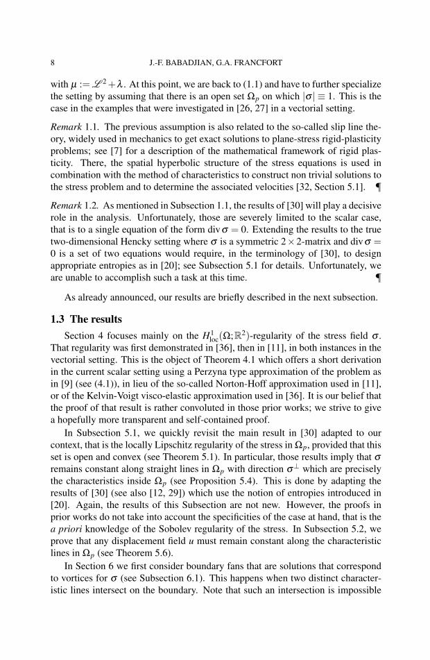
However, there can be a jump on (x,y) ∈ R2 : 0 < x < d, x+ y = ` since, inthat case, σ ·ν = 1. Since d < `, the part U := (x,y) ∈ Ω : d − x < y < `− x isnot traversed by characteristic lines intersecting (0,d)×0 (see Figure 1.1). So,λ (x,y)= ζ (x+y), where ζ is any nonnegative Radon measure. Because w= a`√
2on
(x,y)∈R2 : 0 < x < d, x+y= `, we must have Z+(`) = (a−1)`. In conclusion,Z can be any monotonically increasing function such that Z ≡ 0 on (0,d) andZ+(`) = (a− 1)`. This in turn will give rise to many possible u’s in U through(1.5).
Note that, for d = ` the domain degenerates to a triangle, the Neumann bound-ary condition is only on 0× (0, `) and the solution is unique. It corresponds toZ ≡ 0 on (0, `) and Z+(`) = (a−1)`.
In the spirit our prior discussion, one should investigate the compatibility equa-tion curl Du = 0, that is the continuity equation
curl (µσ) = 0.
8 J.-F. BABADJIAN, G.A. FRANCFORT
with µ :=L 2+λ . At this point, we are back to (1.1) and have to further specializethe setting by assuming that there is an open set Ωp on which |σ | ≡ 1. This is thecase in the examples that were investigated in [26, 27] in a vectorial setting.
Remark 1.1. The previous assumption is also related to the so-called slip line the-ory, widely used in mechanics to get exact solutions to plane-stress rigid-plasticityproblems; see [7] for a description of the mathematical framework of rigid plas-ticity. There, the spatial hyperbolic structure of the stress equations is used incombination with the method of characteristics to construct non trivial solutions tothe stress problem and to determine the associated velocities [32, Section 5.1]. 
Remark 1.2. As mentioned in Subsection 1.1, the results of [30] will play a decisiverole in the analysis. Unfortunately, those are severely limited to the scalar case,that is to a single equation of the form divσ = 0. Extending the results to the truetwo-dimensional Hencky setting where σ is a symmetric 2×2-matrix and divσ =0 is a set of two equations would require, in the terminology of [30], to designappropriate entropies as in [20]; see Subsection 5.1 for details. Unfortunately, weare unable to accomplish such a task at this time. 
As already announced, our results are briefly described in the next subsection.
1.3 The resultsSection 4 focuses mainly on the H1
loc(Ω;R2)-regularity of the stress field σ .That regularity was first demonstrated in [36], then in [11], in both instances in thevectorial setting. This is the object of Theorem 4.1 which offers a short derivationin the current scalar setting using a Perzyna type approximation of the problem asin [9] (see (4.1)), in lieu of the so-called Norton-Hoff approximation used in [11],or of the Kelvin-Voigt visco-elastic approximation used in [36]. It is our belief thatthe proof of that result is rather convoluted in those prior works; we strive to givea hopefully more transparent and self-contained proof.
In Subsection 5.1, we quickly revisit the main result in [30] adapted to ourcontext, that is the locally Lipschitz regularity of the stress in Ωp, provided that thisset is open and convex (see Theorem 5.1). In particular, those results imply that σ
remains constant along straight lines in Ωp with direction σ⊥ which are preciselythe characteristics inside Ωp (see Proposition 5.4). This is done by adapting theresults of [30] (see also [12, 29]) which use the notion of entropies introduced in[20]. Again, the results of this Subsection are not new. However, the proofs inprior works do not take into account the specificities of the case at hand, that is thea priori knowledge of the Sobolev regularity of the stress. In Subsection 5.2, weprove that any displacement field u must remain constant along the characteristiclines in Ωp (see Theorem 5.6).
In Section 6 we first consider boundary fans that are solutions that correspondto vortices for σ (see Subsection 6.1). This happens when two distinct character-istic lines intersect on the boundary. Note that such an intersection is impossible

CONTINUITY EQUATION IN HENCKY PLASTICITY 9
inside Ωp because it would contradict the continuity of σ at that point. Those canbe anywhere in Ωp. We take their union and consider the complementary set Cwithin Ωp. We show that each connected component of C intersects the boundary∂Ωp. If its interior is empty, it is a characteristic line. Otherwise, its intersectionwith ∂Ωp has one or two connected components. Furthermore, if it has two con-nected components, then all points in those are traversed by a characteristic line,whereas if it has only one component, then it might be so that a single line segmentwithin that component is not traversed by any characteristic. This is the object ofTheorem 6.11 which is our main rigidity result. As far as the stress is concerned,we show continuity of the stress at all points of the boundary that are traversed by acharacteristic (see Theorem 6.22). Finally, we demonstrate that, besides boundaryfans, exterior fans (that are fans with an apex outside Ωp), and areas of constant σ
(which correspond to parallel characteristic lines), one can also have areas wherethe characteristic lines look like a “continuous” one parameter family of lines, e.g.of the form y = x/t− t, for t > 0 (see Paragraph 6.3). We conjecture that those foursituations are the only possible ones for σ in the region on which |σ |= 1.
The behavior of any solution field (σ ,u) along the characteristic lines in Ωp (seeProposition 5.4 and Theorem 5.6) seems beyond reach for now, even in the scalar-valued setting, absent an additional assumption like the existence of a set with nonempty interior where |σ | = 1. But even in our restrictive setting this result fallsshort of adjudicating uniqueness of the plastic strain p. This is so because the setP := x ∈ Ω : |σ | = 1 is a closed set in Ω while we have to assume that Ωp is aconvex open set in the interior of P. In particular, we have no systematic way ofrelating the values of u on the boundary of ∂Ω to those on ∂Ωp, except for veryparticular settings (see Propositions 6.3 and 6.23). If Ω was a convex domain andP=Ω, then uniqueness could be obtained, at least in the case of Dirichlet boundaryconditions throughout ∂Ω. For more details see Remark 6.24.
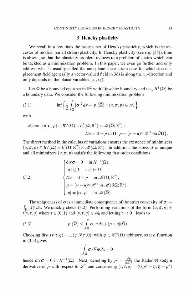
For the reader’s convenience, we concatenate the main results in a unique Theo-rem which, in its concision, somewhat hides the hyperbolic nature of the questionsthat are central to this paper (see Figure 1.2 for an illustration of the geometricstructure of the solutions).
Theorem 1.3 (Main results). Assume that Ω is a Lipschitz bounded domain of R2
and that w ∈ H1(Ω). The minimization problem
inf1
2
ˆΩ
|σ |2 dx+ |p|(Ω) : (u,σ , p) ∈ Aw
with
Aw := (u,σ , p) ∈ BV (Ω)×L2(Ω;R2)×M (Ω;R2) :
Du = σ + p in Ω, p = (w−u)νH 1 on ∂Ω
has at least one minimizer (u,σ , p). Furthermore, σ is unique and belongs toH1
loc(Ω;R2).

10 J.-F. BABADJIAN, G.A. FRANCFORT
•z1
F1
•z2
F2
•z3
F3C1
•
•S1
L
C2 C3
•S3
Ωp
FIGURE 1.2. An example of geometry with three boundary fans F1, F2,F3 with apexes, respectively, z1, z2, z3, three connected components C1,C2 and C3, and a characteristic line L which is the intersecting charac-teristic line segment between the (open) fans F1 and F2. The connectedcomponents C1 and C3 have one characteristic line segment on theirboundaries, the characteristic boundary set S1 is a closed line segment,while S3 is a single point. The connected component C2 has two charac-teristic line segments on its boundary.
Assume moreover that there exists a non empty convex open set Ωp ⊂ Ω suchthat |σ | = 1 a.e. on Ωp. Then σ is locally Lipschitz on Ωp and remains constantalong each open line segment
Lx := (x+Rσ⊥(x))∩Ωp, with x ∈ Ωp,
called a characteristic line segment. Moreover, u remains constant along Lx ∩Ωp for all x ∈ Ωp \ (
⋃z∈Z Lz) where Z ⊂ Ωp is an H 1-negligible set such that
L 2 (⋃
z∈Z Lz ∩Ωp) = 0.Geometrically, Ωp can be decomposed as the following disjoint union
Ωp =⋃i∈I
Fi ∪⋃
λ∈Λ
(Lxλ∩Ωp)∪
⋃j∈J
C j,
for some countable sets I and J, and some (possibly) uncountable set Λ. For alli ∈ I, Fi is a boundary fan, i.e., the intersection of Ωp with an open cone with apexzi ∈ ∂Ωp and two characteristic line segments as generatrices; for all λ ∈ Λ, Lxλ
isa characteristic line segment passing through xλ ∈ Ωp and we set Pλ := Lxλ
∩∂Ωp(a set made of two points); and for all j ∈ J, C j is a convex set, closed in the relativetopology of Ωp and with non empty interior, endowed with one of the following twoproperties:
• Either ∂C j = L j∪Γ j with L j ⊂Ωp an open characteristic line segment andΓ j a connected closed set in ∂Ωp. In that case, Γ j = Γ1
j ∪Γ2j ∪S j where Γ1
j
and Γ2j are connected and S j is a closed line segment (possibly reduced to
single point) that separates Γ1j and Γ2
j . Further each point of Γ1j (resp. Γ2
j)

CONTINUITY EQUATION IN HENCKY PLASTICITY 11
is traversed by a characteristic line segment which will re-intersect ∂Ωp
on Γ2j (resp. Γ1
j);• Or ∂C j = L j ∪L′
j ∪Γ j ∪Γ′j where L j and L′
j ⊂ Ωp are open characteristicline segments, while Γ j and Γ′
j are two disjoint connected closed sets in∂Ωp. Further each point of Γ j (resp. Γ′
j) is traversed by a characteristicline segment which will re-intersect ∂Ωp on Γ′
j (resp. Γ j). In that case weset S j = /0.
Finally, σ is continuous on Ωp \(⋃
λ∈Λ Pλ ∪⋃
j∈J S j ∪⋃
i∈Izi).
Remark 1.4. Our results only pertain to the case ∂Ωd = ∂Ω and ∂Ωn = /0. Thereare no obstacles in treating the more general case of a surface load g on a Neumannpart of the boundary ∂Ωn. This would simply add the term −
´∂Ωn
gudH 1 in theminimization problem (3.1) and the term
´∂Ωn
ϕg(u−w)dH 1 in the definition(2.2) of the duality. However, one would have to spell out a so-called safe-loadconditions on g that guarantee existence, as well as add technical conditions on∂b∂Ω∂Ωd (the boundary of the Dirichlet part ∂Ωd in ∂Ω) (see [24, Section 6]).Barring this, all results are local in nature and would not be affected. With thatcaveat in mind, all our results, which are local, equally hold in the enlarged settingof a Neumann condition on part of the boundary of the domain. 
As already alluded to at the onset of the introduction, the reader uninterested inthe particulars of Hencky plasticity may skip Sections 3, 4 without prejudice andview our contribution as an investigation of the continuity equation (1.1) under theassumptions (1.2) on σ , but with the additional knowledge of the existence of anonnegative measure-solution µ such that σ µ = Du for some u ∈ BV (Ω).
2 Notation and preliminaries
The Lebesgue measure in Rn is denoted by L n and the s-dimensional Haus-dorff measure by H s.
From here onward the space dimension is set to 2. If a and b ∈ R2, we writea ·b for the Euclidean scalar product, and we denote the norm by |a|=
√a ·a. The
open (resp. closed) ball of center x and radius ρ is denoted by Bρ(x) (resp. Bρ(x)).If K ⊂R2 is a closed and convex set, we denote by NK(x) = ξ ∈R2 : ξ ·(y−x)≤0 for all y ∈ K the normal cone to K at x ∈ ∂K, and by TK(x) = ζ ∈R2 : ξ ·ζ ≤0 for all ξ ∈ NK(x) the tangential cone to K at x ∈ ∂K. If z = (z1,z2) ∈ R2, wedenote by z⊥ = (−z2,z1) the rotation of z of an angle π/2. Given two vectors u andv ∈R2, we denote by C(u,v) := αu+βv : α > 0, β > 0 the open cone generatedby u and v with apex at the origin. Also, if f : R→R is a proper, convex function,we denote by ∂ f (x) (or ∂ f (·)(x)) the subdifferential of f at the point x ∈R2 whichis not empty at all points in the interior of its domain.
In all that follows, Ω⊂R2 is a bounded and Lipschitz open set. We use standardnotation for Lebesgue and Sobolev spaces. We write M (Ω;R2) (resp. M (Ω)) for

12 J.-F. BABADJIAN, G.A. FRANCFORT
the space bounded Radon measures in Ω with values in R2 (resp. R), endowedwith the norm |µ|(Ω), where |µ| ∈ M (Ω) is the total variation of the measure µ .The space BV (Ω) of functions of bounded variation in Ω is made of all functionsu ∈ L1(Ω) such that its distributional gradient Du ∈ M (Ω;R2). Then BV (Ω) ⊂L2(Ω).
Given a map σ : R2 → R2, we set divσ := ∂σ1∂x1
+ ∂σ2∂x2
and denote by curlσ the
scalar quantity ∂σ2∂x1
− ∂σ1∂x2
(=−divσ⊥). We denote by H(div,Ω) the Hilbert spaceof all σ ∈ L2(Ω;R2) such that divσ ∈ L2(Ω). We recall that if Ω is bounded withLipschitz boundary and σ ∈ H(div,Ω), its normal trace, denoted by σ ·ν , is welldefined as an element of H−1/2(∂Ω). If further σ ∈ H(div,Ω)∩L∞(Ω;R2), thenσ ·ν ∈ L∞(∂Ω) with ‖σ ·ν‖L∞(∂Ω) ≤ ‖σ‖∞ (see e.g. [3, Theorem 1.2]). Moreover,according to [14, Theorem 2.2 (iii)], if Ω is of class C 2, then for all ϕ ∈ L1(∂Ω),
(2.1) limε→0
ˆ 1
0
ˆ∂Ω
(σ(y− εsν(y)) ·ν(y)− (σ ·ν)(y)
)ϕ(y)dH 1(y)ds = 0,
where ν denotes the outer unit normal to ∂Ω.According to [3, Definition 1.4], we define a generalized notion of duality pair-
ing between stresses and plastic strains as follows (see also [24, Section 6]).
Definition 2.1. Let σ ∈ H(div,Ω)∩L∞(Ω;R2), (u,e, p) ∈ BV (Ω)×L2(Ω;R2)×M (Ω;R2) and w ∈ H1(Ω) be such that Du = e+ p in Ω and p = (w−u)νH 1 on∂Ω. We define the distribution [σ · p] ∈ D ′(R2) by
(2.2) 〈[σ · p] ,ϕ〉=ˆ
Ω
ϕσ · (∇w− e) dx+ˆ
Ω
(w−u)σ ·∇ϕ dx
+
ˆΩ
(w−u)(divσ)ϕ dx for all ϕ ∈ C ∞c (R2).
If Ω has Lipschitz boundary, approximating σ by smooth functions, and us-ing the integration by parts formula in BV , one can show that [σ · p] is actually abounded Radon measure supported in Ω satisfying
(2.3) |[σ · p]| ≤ ‖σ‖∞|p| in M (Ω)
and with total mass that obtained by taking ϕ ≡ 1 in (2.2). Moreover, if σ ∈C (Ω;R2) we can show that
〈[σ · p] ,ϕ〉=ˆ
Ω
ϕσ · d p =
ˆΩ
ϕσ · d pd|p|
d|p| for all ϕ ∈ Cc(Ω),
where d pd|p| stands for the Radon-Nikodým derivative of p with respect to its total
variation |p|. For all of the above, see [24, Section 6] in the vectorial case.
CONTINUITY EQUATION IN HENCKY PLASTICITY 13
3 Hencky plasticity
We recall in a few lines the basic tenet of Hencky plasticity, which is the an-cestor of modern (small strain) plasticity. In Hencky plasticity (see e.g. [38]), timeis absent, so that the plasticity problem reduces to a problem of statics which canbe tackled as a minimization problem. In this paper, we even go further and onlyaddress what is usually called the anti-plane shear strain case for which the dis-placement field (generally a vector-valued field in 3d) is along the x3-direction andonly depends on the planar variables (x1,x2).
Let Ω be a bounded open set in R2 with Lipschitz boundary and w ∈ H1(Ω) bea boundary data. We consider the following minimization problem
(3.1) inf1
2
ˆΩ
|σ |2 dx+ |p|(Ω) : (u,σ , p) ∈ Aw
with
Aw := (u,σ , p) ∈ BV (Ω)×L2(Ω;R2)×M (Ω;R2) :
Du = σ + p in Ω, p = (w−u)νH 1 on ∂Ω.
The direct method in the calculus of variations ensures the existence of minimizers(u,σ , p) ∈ BV (Ω)× L2(Ω;R2)×M (Ω;R2). In addition, the stress σ is uniqueand all minimizers (u,σ , p) satisfy the following first order conditions
(3.2)
divσ = 0 in H−1(Ω),
|σ | ≤ 1 a.e. in Ω,
Du = σ + p in M (Ω;R2),
p = (w−u)νH 1 in M (∂Ω;R2),
|p|= [σ · p] in M (Ω).
The uniqueness of σ is a immediate consequence of the strict convexity of σ 7→´Ω|σ |2 dx. We quickly check (3.2). Performing variations of the form (u,σ , p)+
t(v,τ,q) where t ∈ (0,1) and (v,τ,q) ∈ A0 and letting t → 0+ leads to
(3.3) |p|(Ω)≤ˆ
Ω
σ · τ dx+ |p+q|(Ω).
Choosing first (v,τ,q) = ±(ϕ,∇ϕ,0), with ϕ ∈ C ∞c (Ω) arbitrary, as test function
in (3.3) gives ˆΩ
σ ·∇ϕ dx = 0
hence divσ = 0 in H−1(Ω). Next, denoting by pa = d pdL 2 the Radon-Nikodým
derivative of p with respect to L 2 and considering (v,τ,q) = (0, pa −η ,η − pa)

14 J.-F. BABADJIAN, G.A. FRANCFORT
as test function in (3.3), where η ∈ L1(Ω;R2) is arbitrary, leads toˆΩ
|η |dx ≥ˆ
Ω
|pa|dx+ˆ
Ω
σ · (η − pa)dx.
Localizing this inequality yields σ(x) ∈ ∂ | · |(pa(x)) ⊂ ∂ | · |(0) for a.e. in x ∈ Ω,hence
(3.4) |σ | ≤ 1 a.e. in Ω.
It remains to prove the “flow rule". From (2.3) and (3.4) the first inequality |p| ≥[σ · p] in M (Ω) holds. To prove the reverse inequality take (v,τ,q) = (w−u,∇w−σ ,−p) as test function in (3.3), and use the definition (2.2) of duality. This gives
|p|(Ω)≤ˆ
Ω
σ · (∇w−σ)dx = 〈[σ · p],1〉.
Hence, the nonnegative measure |p|− [σ · p] has zero total mass which leads to theflow rule |p|= [σ · p] in M (Ω).
Remark 3.1. Exactly as in [24, Lemma 3.8], if ω is an open subset of Ω withLipschitz boundary Γ = ∂ω and such that ω ⊂ Ω, then σ ·ν ∈ L∞(Γ) and
[σ · p] Γ = (σ ·ν)(u+−u−)H 1Γ,
where u+ and u− are the outer and inner traces of u on Γ and σ · ν is the normaltrace of σ on Γ. Thus, the flow rule localized on Γ reads
(σ ·ν)(u+−u−) = |u+−u−| H 1-a.e. on Γ.
Since by definition u+ 6= u− on Ju, we infer that σ · ν = ±1 H 1-a.e. on Γ∩ Ju.This applies also if H 1(∂ω ∩∂Ω)> 0, replacing u+ by w on that part of ∂ω . 
4 Sobolev regularity of the stress
This section revolves around the Seregin/Bensoussan-Frehse’s Sobolev regu-larity property of the (unique) stress field σ in the minimization problem (3.1) (orequivalently in the system (3.2)).
Theorem 4.1 (Seregin/Bensoussan-Frehse regularity). The unique stress σ suchthat the triplet (u,σ , p) ∈ BV (Ω)×L2(Ω;R2)×M (Ω;R2) is a minimizer of (3.1)belongs to H1
loc(Ω;R2).
Proof. Step 1. In a first step we perform a so-called Perzyna approximation of theminimization problem (3.1). We thus consider, for ε > 0,
(4.1)
infˆ
Ω
(12|σ |2 + |p|+ ε
2|p|2)
dx : (u,σ , p) ∈ H1(Ω)×L2(Ω;R2)×L2(Ω;R2)
such that ∇u = σ + p a.e. in Ω and u = w H 1-a.e. on ∂Ω
.
By strict convexity, there exists a unique minimizing triplet (uε ,σε , pε).

CONTINUITY EQUATION IN HENCKY PLASTICITY 15
Further, for a subsequence (still labeled by ε), it is straightforward to show that
(4.2)
uε u weak-* in BV (Ω),
σε σ weak in L2(Ω;R2),
(√
ε pε)ε>0 is bounded in L2(Ω;R2),
pε p weakly* in M (Ω;R2),
where (u,σ , p)∈BV (Ω)×L2(Ω;R2)×M (Ω;R2) is a minimizer of (3.1) as can beseen through direct application of an approximation result found in [34, Theorem3.5]; see also [9, Proposition 3.3].
Now, testing minimality with triplets (uε + tv,σε + tτ, pε + tq) with t ∈ (0,1)and (v,τ,q)∈ H1
0 (Ω)×L2(Ω;R2)×L2(Ω;R2) where ∇v = τ +q, it is easily seen –choosing either q ≡ 0 and τ = ∇v with v ∈ H1
0 (Ω) arbitrary, or v ≡ 0 and τ =−q1Ewhere E ⊂ Ω is measurable and q ∈ R2 arbitrary – that the minimizing triplet(uε ,σε , pε) satisfies the following Euler-Lagrange equations:
(4.3)
divσε = 0 in H−1(Ω),
∇uε = σε + pε a.e. in Ω,
uε = w H 1-a.e. on ∂Ω,
σε − ε pε ∈ ∂H(pε) a.e. in Ω,
where H(q) := |q| for all q ∈ R2.
Remark 4.2. Observe that the fourth relation in (4.3) reads, by convex duality, as
pε ∈ ∂ I(σε − ε pε) a.e. in Ω,
where I is the indicator function of the closed unit ball, i.e.,
I(q) :=
0 if |q| ≤ 1,+∞ if |q|> 1.
Thus ∇uε − ε pε = pε +(σε − ε pε) ∈ ∂Ψ(σε − ε pε) where Ψ : R2 → R is definedby
Ψ(q) :=12|q|2 + I(q) for all q ∈ R2,
or still
(4.4) σε − ε pε = DΨ∗(∇uε − ε pε)
where Ψ∗ : R2 → R, the convex conjugate of Ψ, is given by
Ψ∗(q) =
12 |q|
2 if |q| ≤ 1,
|q|− 12 if q|> 1.

16 J.-F. BABADJIAN, G.A. FRANCFORT
Remark that Ψ∗ ∈ C 1(R2) with
DΨ∗(q) =
q if |q| ≤ 1,
q/|q| if |q|> 1,
and that DΨ∗ ∈ Lip(R2)∩C 1(R2 \S1) with
D2Ψ
∗(q) =
Id if |q|< 1,1|q|
Id− 1|q|3
q⊗q if |q|> 1.
Finally, the expression for D2Ψ∗ implies that, for |q|> 1 and for all r ∈ R2,
D2Ψ
∗(q)[r] =1|q|
Pq⊥(r)
where Pq⊥ is the orthogonal projection onto the linear span of q⊥.Those projection properties, which are specific to the Von-Mises criterion, will
be instrumental in the proof of the Sobolev regularity of the stress. 
For ε fixed, a usual translation argument yields the classical local elliptic reg-ularity of the fields (see e.g. [9, Proposition 3.4] in the vectorial evolution case),that is
(4.5) uε ∈ H2loc(Ω), σε , pε ∈ H1
loc(Ω;R2)
with corresponding ε-dependent bounds.
Step 2. Let k ∈ 1,2 and ϕ ∈ C ∞c (Ω). Taking ϕ2∂kuε (which belongs to H1
0 (Ω)thanks to (4.5)) as test function for the equation
div(∂kσε) = 0 in H−1(Ω),
we obtain
0 =
ˆΩ
ϕ2∂kσε ·∂k∇uε dx+
ˆΩ
∂kσε ·∇ϕ2∂kuε dx =: I1 + I2.
In the sequel, Cϕ will stand for a positive constant which may vary from line to line;it may depend on ϕ and on the bounds coming from (4.2), but it is independent ofε .
We now rewrite I1 and I2 as follows.
(4.6) I1 =
ˆΩ
ϕ2|∂kσε |2 dx+
ˆΩ
ϕ2 (∂kσε − ε∂k pε) ·∂k pε dx+ ε
ˆΩ
ϕ2|∂k pε |2 dx,
while
|I2| ≤ 2ˆ
Ω
|∂kσε ·∇ϕ| |(σε)kϕ|dx+ˆ
Ω
|∂kσε ||∇ϕ2||(pε)k|dx
≤ Cϕ‖σε‖L2(Ω)‖ϕ∂kσε‖L2(Ω)+
ˆΩ
|∂kσε ||∇ϕ2||pε |dx.(4.7)

CONTINUITY EQUATION IN HENCKY PLASTICITY 17
Using Young’s inequality and reassembling (4.6), (4.7) we thus get, in view of thebound coming from the second convergence in (4.2),
(4.8)12
ˆΩ
ϕ2|∂kσε |2 dx+ ε
ˆΩ
ϕ2|∂k pε |2 dx+
ˆΩ
ϕ2 (∂kσε − ε∂k pε) ·∂k pε dx
≤Cϕ +
ˆΩ
|∂kσε ||∇ϕ2||pε |dx,
or still, adding and subtracting ∂kσε −ε∂k pε to ∂k pε in the third integral on the lefthand-side of (4.8) above and recalling that ∇uε = σε + pε ,
(4.9)12
ˆΩ
ϕ2|∂kσε |2 dx+ ε
ˆΩ
ϕ2|∂k pε |2 dx
+
ˆΩ
ϕ2(∂kσε − ε∂k pε) · (∂k∇uε − ε∂k pε)dx
≤Cϕ +
ˆΩ
ϕ2|∂kσε − ε∂k pε |2 dx+
ˆΩ
|∂kσε ||∇ϕ2||pε |dx.
We now rewrite (4.9) using Remark 4.2. Since, in view of (4.5), ∇uε − ε pε ∈H1
loc(Ω;R2), we can apply the generalized chain rule formula from [35, Theorem2.1] to (4.4). We obtain
(4.10) ∂kσε − ε∂k pε = D2Ψ
∗(∇uε − ε pε) [∂k∇uε − ε∂k pε ] .
Remark 4.3. Relation (4.10) has to be understood as follows (see [35]):
(4.11) ∂kσε − ε∂k pε =
∂k∇uε − ε∂k pε if |∇uε − ε pε | ≤ 1,1
|∇uε − ε pε |P(∇uε−ε pε )⊥(∂k∇uε − ε∂k pε) else.
Note that application of [35, Proposition 2.2] to the C 1-Lipschitz functions q 7→|q|2 and q 7→ 2|q|−1 yields
∂k∇uε − ε∂k pε =1
|∇uε − ε pε |P(∇uε−ε pε )⊥(∂k∇uε − ε∂k pε)
a.e. on |∇uε − ε pε |= 1,
which implies that (4.11) can be changed into
∂kσε − ε∂k pε =
∂k∇uε − ε∂k pε if |∇uε − ε pε |< 1,1
|∇uε − ε pε |P(∇uε−ε pε )⊥(∂k∇uε − ε∂k pε) else.

18 J.-F. BABADJIAN, G.A. FRANCFORT
In view of (4.10), (4.9) reads as
(4.12)12
ˆΩ
ϕ2|∂kσε |2 dx+ ε
ˆΩ
ϕ2|∂k pε |2 dx+
ˆΩ
ϕ2D2
Ψ∗(∇uε − ε pε)[∂k∇uε − ε∂k pε ] · (∂k∇uε − ε∂k pε)dx
≤Cϕ +
ˆΩ
ϕ2|D2
Ψ∗(∇uε − ε pε)[∂k∇uε − ε∂k pε ]|2 dx
+
ˆΩ
|∂kσε ||∇ϕ2||pε |dx.
Step 3. We next exploit inequality (4.12) obtained at the end of Step 2 by splittingΩ into three ε-dependent subsets as follows,
Ω−ε := x ∈ Ω : |∇uε(x)− ε pε(x)| ≤ 1,
Ω+ε> := x ∈ Ω : |∇uε(x)− ε pε(x)|> 2,
Ω+ε< := x ∈ Ω : 1 < |∇uε(x)− ε pε(x)| ≤ 2,
Ω+ε := Ω
+ε<∪Ω
+ε>.
First note that, on Ω−ε , (4.11) in Remark 4.3 implies that
∂kσε − ε∂k pε = D2Ψ
∗(∇uε − ε pε) [∂k∇uε − ε∂k pε ] = ∂k∇uε − ε∂k pε .
Consequently, the contributions of the integrals involving the term D2Ψ∗(∇uε −ε pε) cancel out on that set in (4.12). Further, writing pε = (∇uε −ε pε)−σε +ε pε
and by virtue of the bounds coming from the second and third convergences in(4.2), we have that,
‖pε‖L2(Ω−ε ∪Ω
+ε<)
≤C
with C > 0 a constant independent of ε (and actually also independent of ϕ). Usingonce again Young’s inequality we can thus absorb the contribution of the term´
Ω−ε ∪Ω
+ε<|∂kσε | |∇ϕ2||pε |dx in the term 1
2
´Ω
ϕ2|∂kσε |2 dx in (4.12) at the possibleexpense of changing Cϕ . In lieu of (4.12), we are thus left with
14
ˆΩ
ϕ2|∂kσε |2 dx+ ε
ˆΩ
ϕ2|∂k pε |2 dx
+
ˆΩ
+ε
ϕ2D2
Ψ∗(∇uε − ε pε)[∂k∇uε − ε∂k pε ] · (∂k∇uε − ε∂k pε)dx
≤Cϕ +
ˆΩ
+ε
ϕ2|D2
Ψ∗(∇uε − ε pε)[∂k∇uε − ε∂k pε ]|2 dx
+
ˆΩ
+ε>
|∂kσε ||∇ϕ2||pε |dx,

CONTINUITY EQUATION IN HENCKY PLASTICITY 19
or still, in view of (4.10), with
14
ˆΩ
ϕ2|∂kσε |2 dx+ ε
ˆΩ
ϕ2|∂k pε |2 dx
+
ˆΩ
+ε
ϕ2D2
Ψ∗(∇uε − ε pε)[∂k∇uε − ε∂k pε ] · (∂k∇uε − ε∂k pε)dx
≤Cϕ +
ˆΩ
+ε
ϕ2|D2
Ψ∗(∇uε − ε pε)[∂k∇uε − ε∂k pε ]|2 dx
+
ˆΩ
+ε>
|D2Ψ
∗(∇uε − ε pε)[∂k∇uε − ε∂k pε ]||∇ϕ2||pε |dx
+ ε
ˆΩ
+ε>
|∂k pε ||∇ϕ2||pε |dx.
Because of the third relation in (4.2) and of Young’s inequality, the third integralin the right hand-side of the last inequality above can be controled by the termε´
Ωϕ2|∂k pε |2 dx in the left hand-side at the expense of changing Cϕ , i.e. ,
(4.13)14
ˆΩ
ϕ2|∂kσε |2 dx+
ε
2
ˆΩ
ϕ2|∂k pε |2 dx
+
ˆΩ
+ε
ϕ2D2
Ψ∗(∇uε − ε pε)[∂k∇uε − ε∂k pε ] · (∂k∇uε − ε∂k pε) dx
≤Cϕ +
ˆΩ
+ε
ϕ2|D2
Ψ∗(∇uε − ε pε)[∂k∇uε − ε∂k pε ]|2 dx
+
ˆΩ
+ε>
|D2Ψ
∗(∇uε −ε pε)[∂k∇uε −ε∂k pε ]||∇ϕ2||∇uε −ε pε |+ |σε +ε pε |
dx,
where we used |pε | ≤ |∇uε − ε pε |+ |σε + ε pε | in the last term of the right handside.
Recalling Remark 4.2 and noting that Pq⊥(ξ ) ·ξ = |Pp⊥(ξ )|2, (4.13) now readsas
14
ˆΩ
ϕ2|∂kσε |2 dx+
ε
2
ˆΩ
ϕ2|∂k pε |2 dx
+
ˆΩ
+ε
ϕ2
|∇uε − ε pε ||P(∇uε−ε pε )⊥ [∂k∇uε − ε∂k pε ]|2 dx
≤Cϕ +
ˆΩ
+ε
ϕ2
|∇uε − ε pε |2|P(∇uε−ε pε )⊥ [∂k∇uε − ε∂k pε ]|2 dx
+
ˆΩ
+ε>
|P(∇uε−ε pε )⊥ [∂k∇uε − ε∂k pε ]||∇ϕ2|dx
+
ˆΩ
+ε>
|∇ϕ2||∇uε − ε pε |
|P(∇uε−ε pε )⊥ [∂k∇uε − ε∂k pε ]||σε + ε pε |dx.

20 J.-F. BABADJIAN, G.A. FRANCFORT
In view of the bounds coming from the second and third relations in (4.2), applica-tion of the Cauchy-Schwarz and Young inequalities to the last term in the inequalityabove yield, at the possible expense of changing Cϕ ,
(4.14)14
ˆΩ
ϕ2|∂kσε |2 dx+
ε
2
ˆΩ
ϕ2|∂k pε |2 dx
+
ˆΩ
+ε
ϕ2
|∇uε − ε pε ||P(∇uε−ε pε )⊥ [∂k∇uε − ε∂k pε ]|2 dx
≤Cϕ +
ˆΩ
+ε<
ϕ2
|∇uε − ε pε |2|P(∇uε−ε pε )⊥ [∂k∇uε − ε∂k pε ]|2 dx
+
ˆΩ
+ε>
|P(∇uε−ε pε )⊥ [∂k∇uε − ε∂k pε ]||∇ϕ2|dx
+32
ˆΩ
+ε>
ϕ2
|∇uε − ε pε |2|P(∇uε−ε pε )⊥ [∂k∇uε − ε∂k pε ]|2 dx.
The second integral in the right hand-side of inequality (4.14) can in turn be esti-mated as follows with the help, once more, of the Cauchy-Schwarz inequality,
ˆΩ
+ε>
|P(∇uε−ε pε )⊥ [∂k∇uε − ε∂k pε ]||∇ϕ2|dx
≤ ‖∇uε − ε pε‖1/2L1(Ω)
ˆΩ
+ε>
|∇ϕ2|2
|∇uε − ε pε ||P(∇uε−ε pε )⊥ [∂k∇uε − ε∂k pε ]|2 dx
1/2
≤C′ϕ
ˆΩ
+ε>
ϕ2
|∇uε − ε pε ||P(∇uε−ε pε )⊥ [∂k∇uε − ε∂k pε ]|2 dx
1/2
,
where the last inequality holds because ‖∇uε −ε pε‖L1(Ω)≤C in view of the boundscoming from (4.2), and C′
ϕ > 0 is another ϕ-dependent constant.

CONTINUITY EQUATION IN HENCKY PLASTICITY 21
Thus inequality (4.14) becomes
(4.15)14
ˆΩ
ϕ2|∂kσε |2 dx+
ε
2
ˆΩ
ϕ2|∂k pε |2 dx
+
ˆΩ
+ε>
ϕ2
|∇uε − ε pε ||P(∇uε−ε pε )⊥ [∂k∇uε − ε∂k pε ]|2 dx
+
ˆΩ
+ε<
ϕ2
|∇uε − ε pε ||P(∇uε−ε pε )⊥ [∂k∇uε − ε∂k pε ]|2 dx
≤Cϕ +32
ˆΩ
+ε>
ϕ2
|∇uε − ε pε |2|P(∇uε−ε pε )⊥ [∂k∇uε − ε∂k pε ]|2 dx
+
ˆΩ
+ε<
ϕ2
|∇uε − ε pε |2|P(∇uε−ε pε )⊥ [∂k∇uε − ε∂k pε ]|2 dx
+C′ϕ
ˆΩ
+ε>
ϕ2
|∇uε − ε pε ||P(∇uε−ε pε )⊥ [∂k∇uε − ε∂k pε ]|2 dx
1/2
.
But |∇uε − ε pε | > 2 on Ω+ε>, while |∇uε − ε pε |2 ≥ |∇uε − ε pε | on Ω
+ε<, so that,
finally, (4.15) implies that
(4.16)14
ˆΩ
ϕ2|∂kσε |2 dx+
ε
2
ˆΩ
ϕ2|∂k pε |2 dx
+14
ˆΩ
+ε>
ϕ2
|∇uε − ε pε ||P(∇uε−ε pε )⊥ [∂k∇uε − ε∂k pε ]|2 dx
≤Cϕ +C′ϕ
ˆΩ
+ε>
ϕ2
|∇uε − ε pε ||P(∇uε−ε pε )⊥ [∂k∇uε − ε∂k pε ]|2 dx
12
.
From a last application of Young’s inequality, it is immediately deduced from(4.16) that the sequence (∂kσε)ε>0 is bounded in H1
loc(Ω;R2) independently of ε ,which implies the desired regularity for ∂kσ . The proof of Theorem 4.1 is com-plete.
Remark 4.4. Since σ ∈ H1loc(Ω;R2), it admits a precise representative defined
Capp-quasi everywhere for any p < 2 hence H s-almost everywhere in Ω for anys > 0 (see e.g. [22, Sections 4.7, 4.8]). In particular, H 1-almost every point in Ω
is a Lebesgue point for σ and satisfies
limρ→0
1ρ2
ˆBρ (x0)
|σ(y)−σ(x)|2 dy = 0 for H 1-a.e. x ∈ Ω.
In the sequel we will identify σ to be its precise representative which is thus definedH 1-almost everywhere in Ω (it is actually defined outside a set of zero Hausdorffdimension). 

22 J.-F. BABADJIAN, G.A. FRANCFORT
Remark 4.5. Arguing as in [4, 16, 25, 9], it is possible to express the flow ruleby means of the quasi-continuous representative of the stress, still denoted by σ ,which is |p|-measurable, in a pointwise sense:
σ(x) · d pd|p|
(x) = 1 for |p|-a.e. x ∈ Ω
or stillp = σ |p| in M (Ω).
In particular, the measure |p| is concentrated in the plastic part of the domain, i.e.,|p|(x ∈ Ω : |σ(x)|< 1) = 0.
Also, the additive decomposition of Du implies that
(4.17) Du = σ + p = σ +σ |p|= σ(L 2 + |p|) in M (Ω).
Remark 4.6. Let S be a segment such that S⊂Ω, then σ ∈H1/2(S;R2). In addition,if x0 ∈ S is a Lebesgue point of σ , then
limρ→0
1ρ
ˆBρ (x)∩S
|σ(y)−σ(x0)|2 dH 1(y) = 0.
In other words, x0 is also a Lebesgue point for the trace of σ on S.
Indeed, the trace theorem in Sobolev spaces states that σ has a trace on S,denoted by σ|S , which belongs to H1/2(S;R2). For simplicity, we will assume thatS = (−1,1)×0. Arguing by approximation, we first observe that, for all x ∈ S,
(4.18)1
4ρ2
ˆx+(−ρ,ρ)2
|σ(y)−σ|S(y1,0)|2 dy ≤Cˆ
x+(−ρ,ρ)2|∇σ(y)|2 dy → 0
as ρ → 0, since ∇σ ∈ L2loc(Ω;M2×2).
Let x ∈ S be a Lebesgue point of σ (as an element of L2L 2(Ω;R2)), i.e.,
(4.19) limρ→0
1ρ2
ˆx+(−ρ,ρ)2
|σ(y)−σ(x)|2 dy = 0
as well as a Lebesgue point of σ|S (as an element of L2H 1(S;R2)), i.e.,
(4.20) limρ→0
1ρ
ˆBρ (x)∩S
|σ|S(y)−σ|S(x)|2 dH 1(y) = 0.
Observe that H 1-almost every point x in S satisfy these properties. As a conse-quence of (4.18) and (4.19), we have
1ρ
ˆBρ (x)∩S
|σ|S(y)−σ(x)|2 dH 1(y) =1ρ
ˆρ
−ρ
|σ|S(y1,0)−σ(x)|2 dy1
≤ 1ρ2
ˆx+(−ρ,ρ)2
|σ(y)−σ|S(y1,0)|2 dy+1
ρ2
ˆx+(−ρ,ρ)2
|σ(y)−σ(x)|2 dy → 0.

CONTINUITY EQUATION IN HENCKY PLASTICITY 23
Using next (4.20), we infer that σ(x) = σ|S(x) which shows that σ = σ|S H 1-a.e.on S, and that σ ∈ H1/2(S;R2).
If now x0 ∈ S is only a Lebesgue of σ , then by (4.18) (which holds for all x0 ∈ S)and (4.19), we have similarly
1ρ
ˆBρ (x0)∩S
|σ(y)−σ(x0)|2 dH 1(y) =1ρ
ˆρ
−ρ
|σ(y1,0)−σ(x0)|2 dy1
≤ 1ρ2
ˆx0+(−ρ,ρ)2
|σ(y)−σ(y1,0)|2 dy+1
ρ2
ˆx0+(−ρ,ρ)2
|σ(y)−σ(x0)|2 dy → 0,
which completes the proof of the result. 
5 Rigidity properties of the solutions
The goal of this section is to take advantage of the hyperbolic equations satisfiedby σ and |p| in the plastic zone x ∈ Ω : |σ(x)| = 1 in order to derive rigidityproperties of the solutions σ and u in that zone. The equations are
(5.1) divσ = 0, |σ |= 1,
and
(5.2) curl (σ(1+ |p|)) = curl Du = 0.
We will need the the following
Hypothesis (H). The set x ∈ Ω : |σ(x)|= 1 has a nonempty interior. We denoteby Ωp a convex open subset of that interior.
Note, for future use, that, in such a setting ∂Ωp has Lipschitz boundary (seee.g. Propositions 2.4.4 and Proposition 2.4.7 in [28]).
As already discussed in the Introduction, hypothesis (H) is fulfilled in severalvectorial examples. It could also be the case in particular in simple scalar settings,for example when Ω itself is a (countable union of) boundary fans (see Subsection6.1).
5.1 Lipschitz regularity and rigidity of the stressIn this subsection we improve the Sobolev regularity of the stress field in the
plastic region. We show that under assumption (H), the stress is actually locallyLipschitz continuous in Ωp, and that it is constant along all the characteristic lines
(5.3) Lx := x+Rσ⊥(x)
for all x ∈ Ωp, associated with the hyperbolic conservation law (5.1) solved by σ
in Ωp. We adopt henceforth the following
Notation. Lx is the characteristic line that passes through x defined as (5.3), thisfor all x ∈ Ωp.

24 J.-F. BABADJIAN, G.A. FRANCFORT
Per hypothesis (H), the systemσ ∈ H1
loc(Ω;R2),
divσ = 0, |σ |= 1 a.e. in Ωp
possesses a solution. The main result of this section is the following
Theorem 5.1 (Jabin-Otto-Perthame regularity). Assume that hypothesis (H) holds.Let ω be a bounded and convex open set such that ω ⊂Ωp and d := dist(ω,∂Ωp)>0. Then, for every Lebesgue points x0 and y0 ∈ ω of σ ,
|σ(x0)−σ(y0)| ≤1d|x0 − y0|.
In particular, σ admits a representative, still denoted by σ , which is locally Lips-chitz in Ωp. Moreover, σ is constant along all characteristic lines Lx0 ∩Ωp, for allx0 ∈ Ωp.
The result was explicitly stated in [29, Theorem 1]. The proof there was in-direct: it used the rigidity result of [30] for general L∞-solutions to the systemdivσ = 0, |σ | = 1. In the sequel, we give a more direct proof of that result by ex-ploiting from the get-go the a priori knowledge of the H1
loc(Ω;R2)-regularity for σ .Doing so simplifies several arguments, for example the existence of traces on lineswhich becomes a straightforward consequence of the trace theorem in Sobolevspaces). The fundamentals of the proof are unchanged. As in [29, 30, 12], theargument rests on the notion of entropies introduced in [20] and on the convexityof the domain, so that we do not claim originality in this Subsection.
Definition 5.2. A function Φ ∈ C ∞c (R2;R2) is called an entropy if, for all z ∈ R2,
z · [DΦ(z)z⊥] = 0, Φ(0) = 0, DΦ(0) = 0.
According to [20, Lemma 2.3], for all entropies Φ, we have div[Φ(σ)] = 0 a.e.in Ωp, or still,
(5.4)ˆ
Ωp
Φ(σ) ·∇ϕ dx = 0
for all test functions ϕ ∈ C ∞c (Ωp). Following [20], we introduce the following
family of parameterized generalized entropies:
Φ(ξ )(z) :=
|z|2ξ if z ·ξ > 0,
0 if z ·ξ ≤ 0,
where ξ ∈ S1. According to [20, Lemma 2.5], there exists a sequence (Φn)n∈N ofentropies in C ∞
c (R2;R2) which is locally uniformly bounded, and such that Φn →Φ(ξ ) pointwise in R2. Specializing (5.4) to Φn and passing to the limit as n →+∞
with the help of Lebesgue’s dominated convergence theorem,

CONTINUITY EQUATION IN HENCKY PLASTICITY 25
ˆΩp
Φ(ξ )(σ) ·∇ϕ dx = 0
for all ξ ∈ S1 and all ϕ ∈ C ∞c (Ωp). Now following [30], we introduce, for a.e.
x ∈ Ωp and for any ξ ∈ S1,
χ(x,ξ ) =
1 if σ(x) ·ξ > 0,0 if σ(x) ·ξ ≤ 0.
The considerations above establish that
div[ξ χ(·,ξ )] = 0 in D ′(Ωp)
for all ξ ∈ S1. This can be rewritten as a so-called kinetic formulation as follows:
Dξ χ(·,ξ ) = 0 in D ′(Ωp).
The previous kinetic formulation entails the ordering property below whoseproof is a direct adaptation of [30, Proposition 3.1] (see also [12, Corollary 4.7]).
Proposition 5.3. Assume that hypothesis (H) holds. Let x0 and y0 ∈ Ωp be twoLebesgue points of σ . Then
σ(x0) · (y0 − x0)> 0 =⇒ σ(y0) · (y0 − x0)≥ 0,
andσ(x0) · (y0 − x0)< 0 =⇒ σ(y0) · (y0 − x0)≤ 0.
Proof. We only prove the first implication. Let us set ξ = y0−x0|y0−x0| . Then
limsupρ→0
L 2(σ ·ξ ≤ 0∩Bρ(x0))
πρ2 σ(x0) ·ξ ≤
limsupρ→0
1πρ2
ˆσ ·ξ≤0∩Bρ (x0)
[σ(x0)−σ(z)] ·ξ dz
≤ limsupρ→0
1πρ2
ˆBρ (x0)
|σ(x0)−σ(z)|dz = 0.
Thus, since σ(x0) ·ξ > 0,
limρ→0
L 2(σ ·ξ ≤ 0∩Bρ(x0))
πρ2 = 0,
hence
limρ→0
L 2(σ ·ξ > 0∩Bρ(x0))
πρ2 = 1.
It shows that x0 is a Lebesgue point of χ(·,ξ ) with χ(x0,ξ ) = 1. Note that the sameargument shows that if σ(x0) ·ξ < 0 then x0 is also a Lebesgue point of χ(·,ξ ) withχ(x0,ξ ) = 0.

26 J.-F. BABADJIAN, G.A. FRANCFORT
Consider the segment S= [x0,y0] and let U = z∈Ωp : dist(z,S)< ε be a (con-nected) ε-neighborhood of S, where ε > 0 is small enough so that S ⊂ U ⊂⊂ Ωp(which is always possible thanks to (H)). Let ηεε>0 be a standard family of molli-fiers and set χε := ηε ∗χ(·,ξ ). Because of the kinetic formulation Dξ χ(·,ξ ) = 0 inD ′(Ωp), then Dξ χε = 0 in U . Thus χε(z) = χε(z+ξ ) for all z ∈U with z+ξ ∈U .Now, x0 is a Lebesgue point of χ(·,ξ ), so that χε(x0)→ χ(x0,ξ ). But y0 = x0+ξ ,so χε(y0) = χε(x0 +ξ ) = χε(x0)→ χ(x0,ξ ) = 1 which implies that σ(y0) ·ξ ≥ 0.Indeed, if we had σ(y0) · ξ < 0, then the above argument would show that y0 is aLebesgue point of χ(·,ξ ) with χ(y0,ξ ) = 0, and thus χε(y0)→ χ(y0,ξ ) = 0 whichis a contradiction.
Thanks to the previous ordering property, we will show that σ is constant onevery line Lx. The following result is an adaptation and an improvement of [30,Proposition 3.2] (see also [12, Proposition 4.8]).
Proposition 5.4. Assume that hypothesis (H) holds. Let x0 ∈ Ωp be a Lebesguepoint of σ . Then σ(x) = σ(x0) for H 1-a.e. x ∈ Lx0 ∩Ωp.
Proof. Up to a change of coordinate system and to a scaling argument, we canassume without loss of generality that x0 = (0,0), Lx0 = Re2, Lx0 ∩Ωp ⊃ 0×[−1,1] := L, that σ(x0) = e1 := (1,0). Let us consider, for ε ∈ (0,1), the triangle
Tε =
y = (y1,y2) ∈ R2 : 0 < y2 < 1 and 0 < y1 <
ε
1− εy2
.
For all Lebesgue points y ∈ Tε of σ , we have
σ(0) · y = y1 > 0
which implies, according to Proposition 5.3, that σ(y) · y ≥ 0. Thus
(5.5) σ2(y)≥−σ1(y)y1
y2≥− ε
1− ε
since |σ1(y)| ≤ 1 and 0 < y1/y2 ≤ ε/(1− ε).Fix η ∈ (0,1/4) and define Sη := 0 × [η ,1 − η ]. Let (0,x2) ∈ Sη be a
Lebesgue point of σ , and consider the half-ball centered at (0,x2) and radius εx2with ε ∈ (0,η), that is
B+ε (x2) = y = (y1,y2) ∈ R2 : y1 > 0 and |y− (0,x2)|< εx2.
It is immediately checked that B+ε (x2)⊂ Tε so that, in view of (5.5),
σ2(y)≥− ε
1− εfor a.e. y ∈ B+
ε (x2).
Then,
− ε
1− ε−σ2(0,x2)≤
2πε2x2
2
ˆB+
ε (x2)|σ2(y)−σ2(0,x2)|dy
so that, because (0,x2) is a Lebesgue point of σ we can pass to the ε 0 limit andwe conclude that σ2(0,x2)≥ 0. A similar argument would show that σ2(0,x2)≤ 0,

CONTINUITY EQUATION IN HENCKY PLASTICITY 27
hence σ2(0,x2) = 0. Recalling Remark 4.4, we get that σ2(0,x2) = 0 for H 1-a.e.(0,x2) ∈ Sη . Since η > 0 is arbitrary, we infer that
σ2 = 0 for H 1-a.e. in 0× (0,1).
The same type of argument would show that
σ2 = 0 for H 1-a.e. in 0× (−1,0).
As a consequence, since |σ |= 1 H 1-a.e. in L, we deduce that
σ = e11A − e11L\A
for some H 1-measurable set A ⊂ L. According to Lemma A.1, the Sobolev spaceH1/2(L;R2) is continuously embedded into VMO(L;R2). Then, we deduce fromLemma A.2 that either H 1(A)= 0 or H 1(L\A)= 0. If H 1(A)= 0, then σ =−e1H 1-a.e. in L so that
−e1 =1
2ρ
ˆL∩Bρ (x0)
σ(y)dH 1(y).
But according to Remark 4.6,
12ρ
ˆL∩Bρ (x0)
σ(y)dH 1(y)→ σ(x0) = e1
which is impossible. As a consequence H 1(L\A) = 0 which implies that σ = e1H 1-a.e. in L as required.
We next show that two distinct characteristic lines cannot intersect inside Ωp.
Proposition 5.5. Assume that hypothesis (H) holds. Let x0 and y0 ∈ Ωp be twoLebesgue points of σ . Then either Lx0 and Ly0 are colinear, or Lx0 ∩ Ly0 = z0where z0 6∈ Ωp.
Proof. If Lx0 and Ly0 are not colinear, we have in particular that σ(x0) 6= σ(y0),σ(x0) 6=−σ(y0) and there exists a unique z0 ∈ Lx0 ∩Ly0 . Assume that z0 ∈ Ωp, andlet z1 ∈ Lx0 ∩Ωp and z2 ∈ Ly0 ∩Ωp be such that the triangle T with vertices z0, z1
and z2 satisfies T ⊂ Ωp. Since σ ∈ H1(T ;R2), its trace σ|∂T∈ H1/2(∂T ;R2). Let
us denote by Sx0 := ∂T ∩Lx0 , Sy0 := ∂T ∩Ly0 and Γ = Sx0 ∪Sy0 so that
σ|∂T∈ H1/2(Γ;R2).
On the other hand, Proposition 5.4 implies that σ|∂T=σ|Sx0
=σ(x0)H 1-a.e. on Sx0
and σ|∂T= σ|Sy0
= σ(y0) H 1-a.e. on Sy0 , which is impossible in view of LemmaA.3. We thus deduce that z0 6∈ Ωp.
A concatenation of the previous results implies the announced local Lipschitzregularity for σ (see [12, Theorem 1.5]).

28 J.-F. BABADJIAN, G.A. FRANCFORT
Proof of Theorem 5.1. Case I: If σ(x0) = σ(y0) then the result follows.
Case II: We now prove that the case σ(x0) =−σ(y0) cannot happen. If σ(x0) ·(y0 − x0) > 0, according to Proposition 5.3, we have σ(y0) · (y0 − x0) ≥ 0 henceσ(x0) · (y0 − x0) ≤ 0 which is impossible. A similar argument shows that σ(x0) ·(y0−x0)< 0 is impossible. It remains to consider the case where σ(x0) ·(y0−x0)=0 which means that y0 ∈ Lx0 =: x0+Rσ⊥(x0) or still that Ly0 = Lx0 . Since x0 and y0are Lebesgue points of σ , we obtain a contradiction with the result of Proposition5.4.
Case III: Assume now that σ(x0) and σ(y0) are not colinear. Then both linesLx0 = x0 +Rσ⊥(x0) and Ly0 = y0 +Rσ⊥(y0) intersect at a single point z0 6∈ Ωp byProposition 5.5. Note that Lx0 (resp. Ly0) is colinear with x0 − z0 (resp. y0 − z0) sothat there is no loss of generality in assuming that e.g.
σ⊥(x0) =
x0 − z0
|x0 − z0|, σ
⊥(y0) =± y0 − z0
|y0 − z0|.
We claim that actually
(5.6) σ⊥(y0) =
y0 − z0
|y0 − z0|.
Since y0 6∈ Lx0 ,
σ(x0) ·y0 − x0
|y0 − x0|6= 0
so that Proposition 5.3 ensures that
(5.7) sign(
σ(x0) ·y0 − x0
|y0 − x0|
)= sign
(σ(y0) ·
y0 − x0
|y0 − x0|
).
Since y0−z0|y0−z0| belongs to the convex cone C( x0−z0
|x0−z0| ,y0−x0|y0−x0|), there exist α > 0 and
β > 0 such thaty0 − z0
|y0 − z0|= α
x0 − z0
|x0 − z0|+β
y0 − x0
|y0 − x0|,
hencey0 − z0
|y0 − z0|· (y0 − x0)
⊥
|y0 − x0|= α
x0 − z0
|x0 − z0|· (y0 − x0)
⊥
|y0 − x0|.
As a consequence
±σ⊥(y0) ·
(y0 − x0)⊥
|y0 − x0|= ασ
⊥(x0) ·(y0 − x0)
⊥
|y0 − x0|or still
(5.8) ±σ(y0) ·y0 − x0
|y0 − x0|= ασ(x0) ·
y0 − x0
|y0 − x0|Gathering (5.7) and (5.8) yields (5.6).
Since dist(z0,ω)≥ d, then it follows that |z0−x0| ≥ d and |z0−y0| ≥ d. There-fore the projections of x0 − z0 and y0 − z0 onto the closed ball Bd(z0) are given,

CONTINUITY EQUATION IN HENCKY PLASTICITY 29
respectively, by d(x0 − z0)/|x0 − z0| and d(y0 − z0)/|y0 − z0|. Since the projectionis 1-Lipschitz, we deduce that
|σ⊥(x0)−σ⊥(y0)|=
∣∣∣∣ x0 − z0
|x0 − z0|− y0 − z0
|y0 − z0|
∣∣∣∣≤ 1d|x0 − y0|,
and the conclusion follows.In the sequel, we will identify σ with its locally Lipschitz representative. In
particular, the conclusion of Proposition 5.3 now holds for all x0 and y0 ∈ Ωp,while that of Proposition 5.4 states that for all x0 ∈ Ωp, then σ(x) = σ(x0) for allx ∈ Lx0 ∩Ωp.
5.2 Rigidity of the displacementWe now demonstrate that the displacement field(s), like the stress field, is (are)
severely constrained by assumption (H) and conform(s) to what formal manipula-tions of the hyperbolic equation (5.2) would entail, that is that the displacementmust remain constant on (almost) every characteristic line in Ωp. Formally, theargument goes as follows. Compute the derivative of u along the characteristics.The chain rule gives
dds
u(x+ sσ⊥(x)) = Du(x+ sσ
⊥(x)) ·σ⊥(x).
Using that σ is constant along the characteristics, we getdds
u(x+ sσ⊥(x)) = Du(x+ sσ
⊥(x)) ·σ⊥(x+ sσ⊥(x)) = 0,
since, thanks to the flow rule, Du = σ(1+ |p|) is colinear with σ . Unfortunately,this argument cannot be made rigorous for want of a general chain rule formula forthe composition of a BV function with a (locally) Lipschitz function.
We will first show that such a property actually holds locally, i.e., for smallvalues of s. Using a well-suited covering we then establish the global result in Ωp,resulting in the
Theorem 5.6. Assume that hypothesis (H) holds. There exists an H 1-negligibleset Z ⊂ Ωp with L 2 ((
⋃z∈Z Lz)∩Ωp) = 0 such that u is constant on Lx∩Ωp for all
x ∈ Ωp \ (⋃
z∈Z Lz).
The rest of the section is devoted to the proof of Theorem 5.6. Let ω be aconvex open set such that ω ⊂ Ωp. Let x0 ∈ ω and R > 0 small enough so thatB2R(x0)⊂ Ωp. Let us define the mapping Φx0 : [−R,R]×R→ R2 by
Φx0(t,s) := x0 + tσ(x0)+ sσ⊥(x0 + tσ(x0)) for all (t,s) ∈ [−R,R]×R.
Clearly, Φx0 is locally Lipschitz in [−R,R]×R as composition of locally Lipschitzmappings.
Proposition 5.7. There exists 0 < r < R and an open neighborhood Ux0 of x0 suchthat the function Φx0 is bi-Lipschitz from Qr := (−r,r)2 onto Ux0 .

30 J.-F. BABADJIAN, G.A. FRANCFORT
Proof. We first observe that, since B2R(x0) ⊂ Ωp and both σ(x0) and σ⊥(x0 +tσ(x0)) are unit vectors, Φx0([−R,R]2) ⊂ Ωp. Moreover, using that σ is locallyLipschitz in Ωp, it follows that t ∈ [−R,R] 7→ σ⊥(x0 + tσ(x0)) is Lipschitz. As aconsequence of Rademacher’s Theorem, it is differentiable almost everywhere andthere exists M > 0 such that
(5.9)∣∣∣∣ ddt
σ⊥(x0 + tσ(x0))
∣∣∣∣≤ M for a.e. t ∈ [−R,R].
Hence, Φx0 is Lipschitz in QR as composition of Lipschitz functions.
Further, Φx0 is injective on QR. Indeed, if (t,s) 6= (t ′,s′) ∈ QR are such thatΦx0(t,s) = Φx0(t
′,s′), then
z := x0 + tσ(x0)+ sσ⊥(x0 + tσ(x0)) = x0 + t ′σ(x0)+ s′σ⊥(x0 + t ′σ(x0)).
Clearly t 6= t ′ and thus x0 + tσ(x0) 6= x0 + t ′σ(x0). The point z would then be-long to both Lx0+tσ(x0) and Lx0+t ′σ(x0) so that, by Proposition 5.5, we would haveLx0+tσ(x0)= Lx0+t ′σ(x0), hence, by Proposition 5.4, σ(x0+tσ(x0))=σ(x0+t ′σ(x0)).But then σ(x0) and σ⊥(x0 + tσ(x0)) are colinear, and, because they are both unitvectors,
(5.10) σ⊥(x0 + tσ(x0)) =±σ(x0).
Consequently, we would have x0 = x0 + tσ(x0)∓ tσ⊥(x0 + tσ(x0)), and the char-acteristic line Lx0+tσ(x0) would intersect Lx0 at the point x0 which is impossible,owing again to Proposition 5.5, unless σ(x0) = ±σ(x0 + tσ(x0)). But this lastrelation contradicts (5.10). The injectivity of Φx0 in QR is established, and, as aconsequence of Brouwer’s Invariance Domain Theorem (see [23, Theorem 3.30]),Φx0 is a homeomorphism from the open square QR onto its range which is open.
We now compute the Jacobian determinant of Φx0 . For a.e. (t,s)∈ QR, we have
det∇Φx0(t,s) = σ(x0) ·σ(x0 + tσ(x0))− sσ⊥(x0 + tσ(x0)) ·
ddt
σ(x0 + tσ(x0))
:= a(t)+ sb(t),(5.11)
where, for a.e. t ∈ (−R,R), we set
a(t) := σ(x0) ·σ(x0 + tσ(x0)), b(t) =−σ⊥(x0 + tσ(x0)) ·
ddt
σ(x0 + tσ(x0)).
Since σ is Lipschitz in B2R(x0), there exists K > 0 such that
(5.12) |σ(x0 + tσ(x0))−σ(x0)| ≤ K|t| for all t ∈ [−R,R].
Thus, by (5.9) and (5.12), for a.e. t ∈ (−R,R),
(5.13) a(t)≥ 1−K|t|, |b(t)| ≤ M,
and we can bound from below the right hand-side of (5.11) by
det∇Φx0(t,s)≥ 1−K|t|−M|s|.

CONTINUITY EQUATION IN HENCKY PLASTICITY 31
Let r > 0 be small enough so that 1− (K +M)r > 12 , then we get that
(5.14) det∇Φx0(t,s)> 1/2 for a.e. (t,s) ∈ Qr.
Denoting by Ux0 := Φx0(Qr)⊂ Ωp, we have so far established that Φx0 : Qr →Ux0
is a Lipschitz homeomorphism. With the help of (5.14), we now show that Φ−1x0
isLipschitz in Ux0 . To that end, we prove in a manner similar to that in [23, Theorem6.1] that Φ−1
x0∈ W 1,∞(Ux0 ;R2). Since we already know that Φ−1
x0is continuous in
Ux0 , it enough to prove that Φ−1x0
has a weak gradient in L∞(Ux0 ;M2×2).Let ϕ ∈ C ∞
c (Ux0) be an arbitrary test function. Using the area formula withthe one-to-one Lipschitz function Φx0 , together with the chain rule formula ∇(ϕ Φx0) = (∇Φx0)
T ∇ϕ Φx0 , we get that for i = 1,2,ˆUx0
Φ−1x0(x)∂iϕ(x)dx =
ˆQr
Φ−1x0(Φx0(t,s))∂iϕ(Φx0(t,s))det∇Φx0(t,s)dt ds
=
ˆQr
[cof(∇Φx0(t,s))∇(ϕ Φx0)(t,s)
]i
(ts
)dt ds.
Let (Φn)n∈N be an approximating sequence in C ∞(Qr;R2) such that Φn → Φx0
uniformly in Qr and also in W 1,p(Qr;R2) for all p < ∞, thenˆUx0
Φ−1x0(x)∂iϕ(x)dx = lim
n→+∞
ˆQr
[cof(∇Φn(t,s))∇(ϕ Φn)(t,s)
]i
(ts
)dt ds.
Integrating by parts, using that div(cof(∇Φn)
)= 0, as well as the area formula
with the function Φx0 once more, we getˆUx0
Φ−1x0(x)∂iϕ(x)dx = − lim
n→+∞
ˆQr
(cof(∇Φn)
)(i)(ϕ Φn)dt ds
= −ˆ
Qr
(cof(∇Φx0)
)(i)(ϕ Φx0)dt ds
= −ˆ
Ux0
(cof(∇Φx0(Φ
−1x0)))(i)
det∇Φx0(Φ−1x0 )
ϕ dx,
where A(i) stands for the i-th row of the matrix A ∈ M2×2. By definition of theweak gradient, (5.14) and since Φx0 is Lipschitz in Qr, we infer that
∇Φ−1x0
=
(cof(∇Φx0(Φ
−1x0)))T
det∇Φx0(Φ−1x0 )
∈ L∞(Ux0 ;M2×2),
which completes the proof of the Proposition.
The mapping Φx0 provides a convenient change of variables thanks to whichwe now deduce that the displacement is locally constant along characteristics.
Proposition 5.8. The function (t,s) ∈ Qr 7→ u Φx0(t,s) ∈ BV (Qr) only dependson t.

32 J.-F. BABADJIAN, G.A. FRANCFORT
Proof. Let (un)n∈N be a sequence in C ∞(Ω)∩W 1,1(Ω) be such that un → u inL1(Ω) and Dun Du weakly* in M (Ω;R2). Let us define the functions
v = uΦx0 , vn = un Φx0 .
Note that vn ∈ W 1,∞(Qr). Because, up to a subsequence, un → u a.e. in Ω andbecause Φ−1
x0, being Lipschitz, maps sets of zero Lebesgue measure into sets of zero
Lebesgue measure, vn → v a.e. in Qr. The area formula (applied to the functionΦx0) together with (5.14) implies that,ˆ
Qr
|vn − v|dt ds =ˆ
Ux0
|un −u|det∇Φx0(Φ
−1x0 )
dx ≤ 2ˆ
Ux0
|un −u|dx → 0.
Hence vn → v in L1(Qr). Since Φx0 ∈W 1,∞(Qr;R2) and ∇vn = (∇Φx0)T ∇un Φx0 ,
the same change of variable argument yields in turnˆ
Qr
|∇vn|dt ds ≤ ‖∇Φx0‖L∞(Qr)
ˆQr
|∇un(Φx0)|dt ds
≤ 2‖∇Φx0‖L∞(Qr)
ˆUx0
|∇un|dx ≤C
for some constant C > 0 independent of n. Hence ∇vnL 2 Dv weakly* inM (Qr;R2) and v ∈ BV (Qr).
Because Φx0 is Lipschitz in Qr, the function
(t,s) ∈ Qr 7→ g(t,s) := det∇Φx0(t,s) = a(t)+ sb(t)
defined in (5.11) is in L∞(Qr) and it is affine with respect to s for a.e. t ∈ (−r,r). Itfollows from an integration by parts that for all ϕ ∈ C ∞
c (Qr)
(5.15)ˆ
Qr
(∂svn)ϕ gdt ds =−ˆ
Qr
((∂sϕ)vn g+ϕ vn ∂sg)dt ds.
On the other hand, using that σ is constant on each characteristic line, i.e., thatσ(x0 + tσ(x0)) = σ(Φx0(t,s)) for all (t,s) ∈ Qr, we get thatˆ
Qr
(∂svn)ϕ gdt ds
=
ˆQr
∇un(Φx0(t,s)) ·σ⊥(x0 + tσ(x0))ϕ(t,s)g(t,s)dtds
=
ˆQr
∇un(Φx0(t,s)) ·σ⊥(Φx0(t,s))ϕ Φ−1x0(Φx0(t,s))g(t,s)dtds
=
ˆUx0
∇un ·σ⊥ϕ Φ
−1x0
dx,(5.16)
where we used once more the area formula with the function Φx0 in the last equality.Since Φ−1
x0is continuous, σ is locally Lipschitz and ϕ ∈ Cc(Qr), it follows that the

CONTINUITY EQUATION IN HENCKY PLASTICITY 33
function σ⊥ϕ Φ−1x0
belongs to Cc(Ux0 ;R2). Gathering (5.15), (5.16), and passingto the limit leads to
−ˆ
Qr
((∂sϕ)vg+ϕ v∂sg)dt ds =ˆ
Ux0
ϕ Φ−1x0
σ⊥ ·dDu.
Because of (4.17), the right-hand side of the previous equality vanishes and
(5.17)ˆ
Qr
((∂sϕ)vg+ϕ v∂sg)dt ds = 0 for all ϕ ∈ C ∞c (Qr).
Since v ∈ BV (Qr), it follows from slicing properties of BV -functions (see [2, The-orem 3.107]) that s 7→ vt(s) = v(t,s) belongs to BV ((−r,r)) for L 1-a.e. t ∈ (−r,r),and, using disintegration, that Dsv = L 1
t ⊗Dvt in M (Qr), i.e.,ˆQr
ϕ dDsv =ˆ r
−r
(ˆ r
−rϕ(t,s)dDvt(s)
)dt for all ϕ ∈ Cc(Qr).
Since s 7→ g(t,s) is affine, we can thus localize (5.17) in t and we conclude that,for L 1-a.e. t ∈ (−r,r),ˆ r
−rg(t,s)φ(s)dDvt(s) = 0 for all φ ∈ Cc((−r,r)),
which means that
(a(t)+ sb(t))Dvt = 0 in M ((−r,r)) for L 1-a.e. t ∈ (−r,r).
Note that by our choice of r and (5.13) a(t)≥ 12 for all t ∈ (−r,r). If b(t) = 0, we
have |a(t)+ sb(t)| = |a(t)| ≥ 12 for all s ∈ (−r,r). On the other hand, if b(t) 6= 0,
we get with (5.13) that ∣∣∣∣a(t)b(t)
∣∣∣∣≥ 12M
.
Since our choice of r ensures that r < 1/2M, we conclude that |a(t)+ sb(t)| > 0for s ∈ (−r,r). We conclude that Dvt = 0 in M ((−r,r)) for L 1-a.e. t ∈ (−r,r),which proves that Dsv = 0 in M (Qr).
We now proceed to the proof of Theorem 5.6.
Proof of Theorem 5.6. Since Uxx∈ω is an open covering of the compact set ω , wecan extract a finite sub-covering. We can thus find finitely many points x1, . . . ,xN ∈ω such that
ω ⊂N⋃
i=1
Uxi .
Let Qi = (−ri,ri)2 = Φ−1
xi(Uxi) be the corresponding open sets with vi := uΦxi ∈
BV (Qi). By Proposition 5.8, Dsvi = 0 in M (Qi), which means that the function
(t,s) ∈ Qi 7→ u(xi + tσ(xi)+ sσ
⊥(xi + tσ(xi)))
34 J.-F. BABADJIAN, G.A. FRANCFORT
is an s-independent BV (Qi)-function. Using slicing properties of BV functions (see[2, Theorem 3.107]), there exists an L 1-negligible set Ni ⊂ (−ri,ri) such that forall t ∈ (−ri,ri)\Ni,
(5.18) s ∈ (−ri,ri) 7→ u(xi + tσ(xi)+ sσ
⊥(xi + tσ(xi)))
is constant.Set Γi = Φxi((−r,r)×0) and Zi := Φxi(Ni ×0). Since L 1(Ni) = 0 and
Φxi is Lipschitz in Qr, H 1(Zi) = 0. Further, since Ωp is bounded, there existsT > 0 large enough so that
⋃z∈Zi
Lz ∩Ωp ⊂ Φxi(Ni × (−T,T )). Using again thatL 1(Ni) = 0, then L 2(Ni × (−T,T )) = 0 and because Φxi is a Lipschitz functionon [−R,R]× [−T,T ], so L 2
((⋃z∈Zi
Lz)∩Ωp
)= 0. From (5.18), for all x ∈ Γi \Zi,
s ∈ (−ri,ri) 7→ u(x+ sσ⊥(x))
is constant. By construction, any point x∈Uxi \(⋃
z∈ZiLz) has an associated charac-
teristic line Lx passing through Γi and, according to Proposition 5.5, Lx∩Lz∩Ωp =/0 for all z ∈ Zi. It thus follows that, for all x ∈Uxi \ (
⋃z∈Zi
Lz), the function
s ∈ (−ri,ri) 7→ u(x+ sσ⊥(x))
is constant, that is u remains constant along Lx ∩Uxi .In turn, Uxi1≤i≤N is a finite covering of ω , so that u is constant on Lx ∩ω for
every x ∈ ω \ (⋃
z∈ZωLz) with Zω :=
⋃Ni=1 Zi satisfying H 1(Zω) = 0 and
L 2
(( ⋃z∈Zω
Lz
)∩Ωp
)= 0.
Finally, consider an exhaustion ωkk∈N of open sets with
ωk =
y ∈ Ωp : dist(x,∂Ωp)>
1k
for all k ≥ 1. Set Z :=
⋃k∈N Zωk which satisfies
H 1(Z) = 0, L 2
((⋃z∈Z
Lz
)∩Ωp
)= 0.
In conclusion, for all x ∈ Ωp \ (⋃
z∈Z Lz), the function u is constant on Lx ∩Ωp.
6 Geometry of the solutions
In this section, we show that assumption (H) constrains the geometric structureof the plastic zone Ωp, and of the solutions (σ ,u) in that set. In particular, sub-sets Fz of Ωp which are bounded by characteristics intersecting at z ∈ ∂Ωp lead toboundary fans where the stress behaves like a vortex centered at the apex z of thefan, and the displacement is a monotone function of the angle (see Theorem 6.2).The complementary of those fans is made of either isolated characteristic lines (seeProposition 6.5), or convex sets C with one or two characteristics on the boundary

CONTINUITY EQUATION IN HENCKY PLASTICITY 35
(see Theorem 6.11). In any case, if the non characteristic boundary of either Fz, orC intersects the boundary of the domain Ω on a set of positive H 1 measure, thenthe propagation of the prescribed Dirichlet boundary datum w through the charac-teristics inside Fz or C provides a partial uniqueness property of the displacement(see Propositions 6.3 and 6.23). In the case of a connected component which is nota boundary fan, possible geometries are offered in Subsection 6.3. They consistof exterior fans (Proposition 6.25), constant zones (Proposition 6.27), or smoothone-parameter families of lines (see Paragraph 6.3). We conjecture that those arethe only possibilities.
6.1 Boundary fansWe set
F :=
z ∈ ∂Ωp : ∃x,y ∈ Ωp with y 6= x such that Lx ∩Ly = z.
It is the set of all points on ∂Ωp belonging to (at least) two distinct characteristiclines. The next result shows that any such point is the apex of a cone which is theunique intersection point of all other characteristic lines inside the cone.
Lemma 6.1. Let z ∈ F and x, y ∈ Ωp with y 6= x be such that Lx ∩Ly = z. Thenfor all z ∈ (z+C(x− z,y− z))∩Ωp,
Lz ∩Lx = Lz ∩Ly = Lx ∩Ly = z.
Proof. Since from hypothesis (H) the set Ωp is assumed to be convex, there existunique points x′ ∈ ∂Ωp ∩Lx and y′ ∈ ∂Ωp ∩Ly with x′ 6= z and y′ 6= z with the opensegments ]z,x′[ and ]z,y′[ contained in Ωp. Let us consider the (closed) triangleT := (x′,y′, z)⊂ Ωp.
If z ∈ T , the line Lz passing through z must intersect at least one of the segments[z,x′[ or [z,y′[. Without loss of generality, we suppose that [z,x′[∩Lz 6= /0 and let z ∈[z,x′[∩Lz. Let us assume that z 6= z. Since Lz ∩Lx = z, we get from Proposition5.5 that z 6∈ Ωp which contradicts the fact that z ∈ ]z,x′[ ⊂ Ωp. Thus z = z and Lzpasses through z.
If z 6∈ T , take any point w on ]z,z[ ∩ T . Then, according to the previous ar-gument Lw passes through the point z, thus [z,w] ⊂ Lw and z ∈ Lw. Therefore,Proposition 5.4 ensures that Lw = Lz, hence Lz passes through z as well.
For all z ∈ F , we consider the set of all points z in Ωp such that the associatedcharacteristic line Lz passes through the point z, i.e.,
Fz := intz ∈ Ωp : z ∈ Lz.
In view of Lemma 6.1, it is a non empty open set of the form Fz := (z+C(x− z,y−z))∩Ωp, for some x,y ∈ Ωp, and we call that open subset of Ωp a boundary fan(see Figure 6.1). Note that it might be the case that [z,x] ⊂ ∂Ωp or [z,y] ⊂ ∂Ωp.In addition, if Fz and Fz′ are two distinct boundary fans, for some z and z′ ∈ F
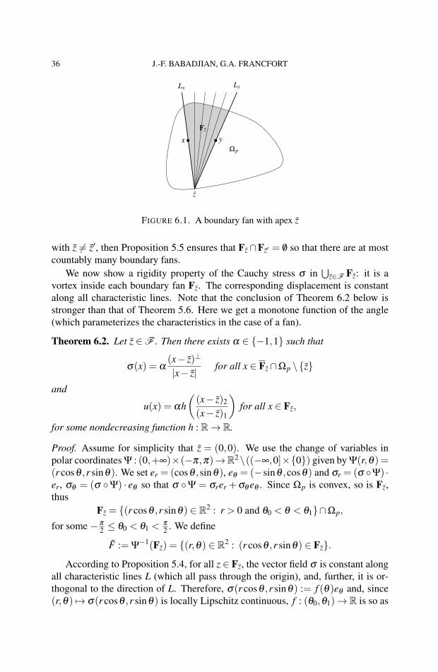
36 J.-F. BABADJIAN, G.A. FRANCFORT
•x • yFz
Ωp
z
Lx Ly
FIGURE 6.1. A boundary fan with apex z
with z 6= z′, then Proposition 5.5 ensures that Fz ∩Fz′ = /0 so that there are at mostcountably many boundary fans.
We now show a rigidity property of the Cauchy stress σ in⋃
z∈F Fz: it is avortex inside each boundary fan Fz. The corresponding displacement is constantalong all characteristic lines. Note that the conclusion of Theorem 6.2 below isstronger than that of Theorem 5.6. Here we get a monotone function of the angle(which parameterizes the characteristics in the case of a fan).
Theorem 6.2. Let z ∈ F . Then there exists α ∈ −1,1 such that
σ(x) = α(x− z)⊥
|x− z|for all x ∈ Fz ∩Ωp \z
and
u(x) = αh((x− z)2
(x− z)1
)for all x ∈ Fz,
for some nondecreasing function h : R→ R.
Proof. Assume for simplicity that z = (0,0). We use the change of variables inpolar coordinates Ψ : (0,+∞)×(−π,π)→R2\((−∞,0]×0) given by Ψ(r,θ)=(r cosθ ,r sinθ). We set er = (cosθ ,sinθ), eθ = (−sinθ ,cosθ) and σr = (σ Ψ) ·er, σθ = (σ Ψ) · eθ so that σ Ψ = σrer +σθ eθ . Since Ωp is convex, so is Fz,thus
Fz = (r cosθ ,r sinθ) ∈ R2 : r > 0 and θ0 < θ < θ1∩Ωp,
for some −π
2 ≤ θ0 < θ1 <π
2 . We define
F := Ψ−1(Fz) = (r,θ) ∈ R2 : (r cosθ ,r sinθ) ∈ Fz.
According to Proposition 5.4, for all z ∈ Fz, the vector field σ is constant alongall characteristic lines L (which all pass through the origin), and, further, it is or-thogonal to the direction of L. Therefore, σ(r cosθ ,r sinθ) := f (θ)eθ and, since(r,θ) 7→ σ(r cosθ ,r sinθ) is locally Lipschitz continuous, f : (θ0,θ1)→R is so as
CONTINUITY EQUATION IN HENCKY PLASTICITY 37
well. Using that |σ | = 1 together with the expression of the divergence in polarcoordinates, we conclude that
| f |= 1 in (θ0,θ1) and f ′ = 0 a.e. in (θ0,θ1),
i.e., f ≡ 1 or f ≡ −1. Therefore, σ Ψ = αeθ , with α = 1 or −1. Comingback to cartesian coordinates leads to the desired expression for σ in Fz, hence toFz ∩Ωp \z by continuity.
Recalling (4.17) Du = σ µ in M (Ωp) with µ := L 2 + |p|. Applying the curlto the previous equality yields
(6.1) 0 = curl(σ µ) = div(σ⊥µ) in D ′(Ωp).
Let µ = Ψ−1 # µ ∈M (F) be the push-forward of µ by Ψ−1. Since σ⊥(x) =−αx|x|
for all x ∈ Fz \z, (6.1) is easily seen to imply that Dr µ = 0 in D ′(F) upon test-ing Dr µ by smooth functions of the form ϕ Ψ =: ϕ ∈ C ∞
c (F). This impliesthe existence of an orthoradial nonnegative measure η ∈ M ((θ1,θ2)) such thatµ = L 1
r ⊗η , i.e., for all ϕ ∈ C ∞c (Fz),ˆ
Fz
ϕ dµ =
ˆF
ϕ dµ =
ˆF
ϕ(r,θ)dr dη(θ),
where, once again, ϕ Ψ = ϕ . As a consequence, since Du = σ µ = αx⊥|x| µ , we
deduce that
(6.2)ˆ
Fz
ϕ dDu = α
ˆF
ϕ(r,θ)eθ dr dη(θ).
But, ˆFz
ϕ dDu = −ˆ
Fz
u∇ϕ dx
= −ˆ
Fu(r cosθ ,r sinθ)∇ϕ(r cosθ ,r sinθ)r dr dθ
= −ˆ
Fu[
Drϕ er +1r
Dθ ϕ eθ
]r dr dθ ,(6.3)
where we set u := u Ψ. Since F does not contain the exceptional line (−∞,0]×0, it follows that Ψ defines a C ∞-diffeomorphism between F and Fz so thatu ∈ BV (F). Thus, since ∂rer = 0, ∂θ eθ =−er, (6.3) reads as
(6.4)ˆ
Fz
ϕ dDu = 〈(Dr(ru)− u)er +(Dθ u)eθ , ϕ〉= 〈(rDru)er +(Dθ u)eθ , ϕ〉,
and gathering (6.2) and (6.4) yields
rDru = 0, Dθ u = αL 1r ⊗η in D ′(F).
By the first equation, there exists an orthoradial function h ∈ BV ((θ0,θ1)) suchthat u(r,θ) = α h(θ) for a.e. (r,θ) ∈ F . The second equation leads to Dh = η ≥ 0

38 J.-F. BABADJIAN, G.A. FRANCFORT
which implies that h is nondecreasing. Using that θ = arctan((x−z)2(x−z)1
)and setting
h = h arctan, the result then follows coming back to cartesian coordinates.
In the following result, we prove a partial uniqueness result for a fan for whicha portion of its “top" boundary coincides with that of Ω, which of course may nothappen.
Proposition 6.3. Extend u by w outside Ω. Let Fz be a fan centered at z ∈ F .Then, u+ = u− H 1-a.e. on ∂Fz ∩ ∂Ωp and, in particular, u = w H 1-a.e. on∂Fz ∩∂Ωp ∩∂Ω.
Proof. Let Cz := z+C(x− z,y− z), for some x, y ∈ Ωp, be the maximal open conewith vertex z such that Fz =Cz ∩Ωp. Then the set ∂Fz ∩Cz = ∂Ωp ∩Cz is open inthe relative topology of ∂Ωp and Lipschitz. According to Remark 3.1, σ ·ν =±1H 1-a.e. on ∂Fz ∩Cz ∩ Ju. Using the explicit expression of σ on Fz \z given byTheorem 6.2, we deduce that σ ·ν coincides H 1-a.e. with the usual scalar productof σ and ν on ∂Fz ∩Cz. Therefore, ν =±σ H 1-a.e. on ∂Fz ∩Cz ∩ Ju.
Assume that H 1(∂Fz ∩Cz ∩ Ju)> 0, since H 1 almost every point of ∂Fz ∩Czis a differentiability point of the boundary, we can find some x0 ∈ ∂Fz ∩Cz ∩ Jusuch that, up to a change of sign, ν(x0) = σ(x0). Let us consider the characteristicline Lx0 = x0 +Rσ⊥(x0) which passes through the point z (because x0 ∈ Fz), andlet H be the closed half plane such that ∂H = Lx0 which does not contain σ(x0) (sothat σ(x0) is the outer unit normal to H). Since σ(x0) is also the unit outer normalto Ωp at x0, it results from the convexity of Ωp that Ωp ⊂ H. Note that since x0 ∈Czwhich is open, then the point x0 does not belong to the boundary of the cone Cz.Hence C′
z := H ∩Cz is a cone with vertex z strictly contained in Cz which satisfies
Fz =C′z ∩Ωp,
which implies that either x or y does not belong to Ωp, a contradiction. This ar-gument proves that H 1(∂Fz ∩Cz ∩ Ju) = 0 and thus, that u+ = u− H 1-a.e. on∂Fz∩Cz. Since in particular H 1((∂Fz∩∂Ωp)\(∂Fz∩Cz)) = 0 the result follows.
Finally, using the boundary condition, we get that u = w H 1-a.e. on ∂Fz ∩∂Ωp ∩∂Ω.
6.2 Outside the fansThe complementary set to the boundary fans, i.e.,
C := Ωp \( ⋃
z∈F
Fz
)is a closed set in the relative topology of Ωp.

CONTINUITY EQUATION IN HENCKY PLASTICITY 39
Topological structure of the complementary of the fans
We first establish topological properties of the connected components of C ,which are closed in the relative topology of Ωp.
Lemma 6.4. Let C be a connected component of C . Then C is convex and for allx ∈ C, Lx ∩Ωp ⊂ C.
Proof. The proof is divided into three steps.
Step 1. We show that, for all x ∈ C , Lx ∩Ωp ⊂ C .Let x ∈C , and consider the characteristic line Lx passing through x. Assume by
contradiction that there exists y ∈ Lx∩Ωp such that y 6∈C . Then Lx = Ly accordingto Theorem 5.1 and, since y /∈ C , there exists z ∈ F such that y ∈ Fz. Thus x ∈Lx ∩Ωp = Ly ∩Ωp ⊂ Fz which is impossible.
Step 2. We show that, for all x ∈ C, Lx ∩Ωp ⊂ C.Consider the characteristic line Lx passing through x. We already know from
the previous step that Lx ∩Ωp ⊂ C . We assume by contradiction that there existsy ∈ Lx ∩Ωp such that y 6∈ C. Let Cy be the connected component of C whichcontains y. We distinguish two cases:
• If the segment [x,y]⊂C , then the closed set C′=C∪[x,y]∪Cy is connected(because [x,y]∩C 6= /0 and [x,y]∩Cy 6= /0), C′ ⊂ C and x, y ∈C′. Then C′
is a connected subset of C which strictly contains C, a contradiction.• If there is z ∈ [x,y] such that z 6∈ C , then we can find z ∈ F such that
z ∈ Fz, which implies, by definition of a fan, that the line Lx = Lz must passthrough the vertex z of the fan Fz and Lx ∩Ωp ⊂ Fz. In particular the pointx belongs to Fz which is again impossible since x ∈ C .
Step 3. We show that C is convex.Let x and y ∈ C, and let us consider a point z ∈ [x,y]. Note that since Ωp is
convex, then z ∈ Ωp and it makes sense to consider its associated characteristic lineLz. If, for all z′ ∈ Lz ∩Ωp, z′ 6∈ C, it would then imply that C ⊂ H+∪H−, whereH± are both open half planes separated by the line Lz. Since both x and y belongto C, the segment [x,y] is not contained in Lz. Then, up to a permutation, x ∈ H−
and y ∈ H+, so that C∩H− 6= /0 and C∩H+ 6= /0. This last property contradictsthe connectedness of C. Therefore, there exists z′ ∈ Lz ∩Ωp such that z′ ∈ C, and,by Step 2, we have Lz ∩Ωp = Lz′ ∩Ωp ⊂ C which implies that z ∈ C. The proof ofthe lemma is complete.
The following result shows that connected components of C with empty interiorare actually characteristic lines.
Proposition 6.5. Let C be a connected component of C be such that C = /0, thenC = Lx ∩Ωp for some x ∈ C.

40 J.-F. BABADJIAN, G.A. FRANCFORT
Proof. Since C 6= /0 there exists x ∈ C and, by Lemma 6.4, Lx ∩ Ωp ⊂ C. Byconvexity of Ωp, the line Lx must intersects ∂Ωp at two distinct points denoted byx′ and x′′, and thus, ]x′,x′′[= Lx ∩Ωp ⊂ C. Assume by contradiction that there isy ∈ C \ (Lx ∩Ωp). The same argument shows that Ly ∩Ωp =]y′,y′′[⊂ C. SinceC is closed in Ωp and convex, and since x′, x′′, y′ and y′′ ∈ C then C containsthe closed and convex hull of x′,x′′,y′,y′′ denoted by convx′,x′′,y′,y′′. ThusC ⊃ int convx′,x′′,y′,y′′ 6= /0 which is against the hypothesis, and finally C =Lx ∩Ωp.
Remark 6.6. Note that there might be uncountably many such characteristic linescorresponding to connected components of C with empty interior. 
We next focus on the (countably many) connected components C of C withnon empty interior. Since σ is constant on each characteristic line inside C, we cannaturally extend σ to the part of boundary of C which is reached by a characteristiccoming from the interior of C, i.e., ∂C∩
⋃z∈C Lz. Specifically, we set
σ(x) = σ(z), Lx := Lz if x ∈ ∂C∩Lz,
in such a way that σ is constant on each Lz ∩C. The value of σ at x is unambigu-ous because there cannot be more than one characteristic line Lz coming from theinterior of C and passing through x, lest x be the apex of a boundary fan containedin C.
Characteristic boundary points
We introduce the set of characteristic boundary points which are the points in∂C not crossed by a characteristic line coming from the interior of C.
Definition 6.7. Let C be a connected component of C be such that C 6= /0. We saythat x ∈ ∂C∩ ∂Ωp is a characteristic boundary point of C if x 6∈ Lz for all z ∈ C.We denote by ∂ cC the set of all characteristic boundary points.
The following result formalizes the idea that the set ∂ cC of all characteristicboundary points of C is made of points where the stress is normal to ∂C, or, equiv-alently, where the characteristics are tangential to ∂C. Note that σ ∈ H1
loc(Ω;R2)∩L∞(Ω;R2) so that, through a sequence of smooth approximations, σ is easilyseen to be well defined on Ω∩∂Ωp as an element of H1/2
loc (Ω∩∂Ωp;R2)∩L∞(Ω∩∂Ωp;R2) (see for example [16, Lemma 2.3]). On the other hand, strictly speaking,σ might not be defined on ∂Ω∩∂Ωp. However, since σ ∈ H(div,Ω)∩L∞(Ω;R2),the normal trace σ ·ν is well defined as an element of H−1/2(∂Ω;R2)∩L∞(∂Ω;R2)through similar arguments.
Proposition 6.8. Let C be a connected component of C be such that C 6= /0 andx ∈ ∂C∩∂Ωp.

CONTINUITY EQUATION IN HENCKY PLASTICITY 41
(i) If x ∈ ∂ cC is an accumulation point of (∂C∩∂Ωp)\∂ cC, denoting by Σ(x)the set of all limits of sequences (σ(xn))n∈N where (xn)n∈N ⊂ ∂C∩∂Ωp \∂ cC is such that xn → x, then
Σ(x)⊂ NC(x)∪ (−NC(x)).
(ii) Assume that the relative interior (∂C∩ ∂Ωp) of ∂C∩ ∂Ωp is not empty
and take x in that set. If x is not an accumulation point of (∂C∩ ∂Ωp) \∂ cC, then x ∈ ∂ cC and there exists a maximal open set Ux containing xsuch that Sx := (∂C∩ ∂Ωp)∩Ux is an open line segment with Sx ⊂ ∂ cC.In addition σ ·ν = 1 or σ ·ν =−1 H 1-a.e. on Sx.
Proof. Step 1. We first assume that x ∈ ∂ cC is an accumulation point of (∂C∩∂Ωp) \ ∂ cC and consider ξ ∈ Σ(x). It means that there exists a sequence (xn)n∈Nin (∂C∩∂Ωp)\∂ cC such that xn → x and σ(xn)→ ξ . By convexity of C, for eachn ∈N, there exists another point yn 6= xn in ∂C∩Lxn . Up to a subsequence, we canassume that yn → y ∈ ∂C. Let us distinguish two possibilities:
Case I. Assume first that x 6= y and that there exists δ > 0 such that for eachn ∈ N,
maxz∈[xn,yn]
dist(z,∂C∩∂Ωp)≥ δ > 0.
Therefore, there is zn ∈ [xn,yn] such that dist(zn,∂C∩∂Ωp)≥ δ and, by compact-ness, up to a further subsequence, we can assume that zn → z for some z ∈ C withdist(z,∂C∩∂Ωp)≥ δ . Since σ is constant along Lxn , we can write
(6.5) xn = zn +θnσ⊥(zn)
for some θn ∈ R. Using that |σ(zn)| = 1, up to a further subsequence we can alsoassume that θn → θ so that, passing to the limit in (6.5) and using the continuity ofσ in Ωp yields x = z+θσ⊥(z), hence x ∈ Lz which is against x ∈ ∂ cC. It showsthat this first possibility never occurs.
Case II. We next suppose that x 6= y and that, for a subsequence
maxz∈[xn,yn]
dist(z,∂C∩∂Ωp)→ 0.
Since xn → x and yn → y, then [xn,yn]→ [x,y] in the sense of Hausdorff. Therefore,for all z ∈ [x,y], there is zn ∈ [xn,yn] such that zn → z. In particular, dist(zn,∂C∩∂Ωp)→ 0 which leads to z∈ ∂C∩∂Ωp. This implies that [x,y]⊂ ∂C∩∂Ωp. Sinceσ(xn) is orthogonal to [xn,yn] for each n ∈ N, we deduce that ξ is orthogonal to[x,y], hence ξ belongs to NC(x)∪ (−NC(x)).
Case III. We finally assume that x = y. Because of the convexity of C, itsboundary ∂C is Lipschitz continuous and thus, there exist r > 0 and a L-Lipschitzfunction f : R→ R such that, in a suitable coordinate system,
C∩Br(x) = (s1,s2) ∈ Br(x) : s2 < f (s1),∂C∩Br(x) = (s1,s2) ∈ Br(x) : s2 = f (s1).

42 J.-F. BABADJIAN, G.A. FRANCFORT
Since limn xn = limn yn = x, we can assume that n is large enough so that xn andyn ∈ Br(x), hence xn = (sn, f (sn)) and yn = (tn, f (tn)). Let Hn be a half plane suchthat ∂Hn = Lxn and Hn does not contain the portion of ∂C in between xn and yn.Let us denote by ξn be the unit exterior normal to Hn and let us fix y ∈ C (seeFigure 6.2). Clearly, if y ∈ C∩Hn, then ξn · (y− xn) ≤ 0. On the other hand, if
•x
•xn
•ynLxn
Hn
•y′n
•y
C
Br(x)
ξn
FIGURE 6.2. The case where x ∈ ∂C∩ ∂Ωp is an accumulation pointof (∂C∩ ∂Ωp) \ ∂ cC, and x = limn xn = limn yn where xn 6∈ ∂ cC andxn 6= yn ∈ Lxn ∩∂C
y ∈ C\Hn we consider the point y′n ∈ ∂C∩ (xn +R∗+(y− xn)) which can be written
as y′n = (t ′n, f (t ′n)). Then, using the convexity of C, we get that
ξn · (y− xn) ≤ ξn · (y′n − xn)≤ |y′n − xn|= |(t ′n, f (t ′n))− (sn, f (sn))|
≤√
1+L2|t ′n − sn| ≤√
1+L2|xn − yn| → 0.
Thus, for all y ∈ C, we have ξn · (y− xn) ≤√
1+L2|xn − yn|. Denoting by ξ anyaccumulation point of the sequence (ξn)n∈N, we infer that
ξ · (y− x)≤ 0 for all y ∈ C,
which means that ξ ∈ NC(x). Since σ(xn) = ±ξn, the previous argument showsthat ξ =±ξ and thus that Σ(x)⊂ NC(x)∪ (−NC(x)).
Step 2. If x is not an accumulation point of (∂C ∩ ∂Ωp) \ ∂ cC, for R > 0small enough, BR(x)∩ (∂C∩ ∂Ωp) \ x ⊂ ∂ cC. By convexity of C and Ωp andsince x ∈ (∂C∩ ∂Ωp)
, R can also be chosen such that there exist two distinctpoints x′ and x′′ such that (∂C∩ ∂Ωp)∩ ∂BR(x) = x′,x′′. Let CR be the convexset delimited by the segment [x′,x′′] and BR(x)∩ (∂C∩ ∂Ωp) (see Figure 6.3). IfBR(x)∩(∂C∩∂Ωp) 6= [x′,x′′], then CR has nonempty interior and, for every y ∈ CR,the characteristic line Ly passing through y must intersect BR(x)∩ (∂C∩ ∂Ωp).Since, except for the point x, this set is contained in ∂ cC, the only possible inter-section point is x. But then x would be the apex of a boundary fan contained in C,which is impossible.
As a consequence, we must have that BR(x)∩ (∂C∩∂Ωp) = [x′,x′′] is a closedline segment. Note that x ∈ [x′,x′′] must belong to ∂ cC. Indeed, if not, let Lz be

CONTINUITY EQUATION IN HENCKY PLASTICITY 43
a characteristic line such that x ∈ Lz for some z ∈ C. Let us consider a triangleT with apexes x, a ∈ Lz and b ∈ ]x,x′[ in such a way that T ⊂ C (see Figure 6.4).Then for any y ∈ T , the associated characteristic line Ly must pass through thepoint x (because ]x,a[⊂ Lz and ]x,b[⊂ ]x,x′[⊂ ∂ cC). Then x would be the apex ofa boundary fan contained in C which is impossible. We have thus established thatthe full segment [x′,x′′] is contained in ∂ cC. The maximal open set Ux is obtainedby taking the union of all open balls BR(x) such that BR(x)∩ (∂ cC∩ ∂Ωp) is asegment.
•x
•x′
•x′′
C
CR
BR(x)
FIGURE 6.3. The casewhere CR 6= /0 leading to acontradiction
•x•x′
•x′′
C
BR(x)Lz
•z
•a•b T
FIGURE 6.4. The casewhere CR = /0, hence[x′,x′′]⊂ ∂C∩∂Ωp
In order to show that σ ·ν = 1 or σ ·ν =−1 H 1-a.e. on Sx, we assume withoutloss of generality that Sx = 0× (−1,1) and that ν = e1 in such a way that C ⊂R−×R. Since Sx ⊂ ∂ cC, then no characteristic line from a point in C intersectsSx. Thus, if δ ∈ (0,1/2), t ∈ (0,1) and y ∈ (−1+δ ,1−δ ), then (−tε,y) ∈ C forε > 0 small enough, and the characteristic line L(−tε,y) passing through the point(−tε,y) intersects the vertical line 0×R at a point (0,yε
0) with |yε0| ≥ 1, or else
σ⊥(−tε,y) =±e2. Since (−tε,y) and (0,yε0)∈ L(−tε,y) = (−tε,y)+Rσ⊥(−tε,y),
then
σ⊥(−tε,y) =
±1√t2ε2 +(yε
0 − y)2
(tε
yε0 − y
)or ± e2 →±e2
as ε → 0.If σ⊥(−tε,y) =±e2 for some y, then σ⊥(−tε,z) =±e2 for all z∈ (−1+δ ,1−
δ ) because (−tε,z)∈ L(−tε,y). Assume that there exist y 6= z∈ (−1+δ ,1−δ ) suchthat σ⊥(−tε,y)→ e2 and σ⊥(−tε,z)→−e2 as ε → 0. Then, denoting by (0,y0)(resp. (0,z0)) the intersection point of L(−tε,y) (resp. L(−tε,z)) with the vertical line0×R, it means that y0 ≥ 1 and z0 ≤ −1. We thus get that both characteristiclines L(−tε,y) and L(−tε,z) intersect at a point x = (x1,x2) with −1+δ ≤ x2 ≤ 1−δ
and − tεδ≤ x1 ≤ 0 (see Figure 6.5).
Thus, for ε > 0 small enough we infer that x ∈ C which is impossible accordingto Proposition 5.5.

44 J.-F. BABADJIAN, G.A. FRANCFORT
• y0
• (0,1)
• (0,0)
• (0,−1)• z0
• (−εt,y)
L(−εt,y)
• (−εt,z)
L(−εt,z)
•xC
FIGURE 6.5.
As a consequence, we always have that
σ((0,y)− εte1) · e1 → 1 or σ((0,y)− εte1) · e1 →−1
for all (t,y)∈ (0,1)×(−1+δ ,1−δ ). Thus in any case, according to the dominatedconvergence theorem,
(6.6) limε→0
ˆ 1
0
ˆ 1−δ
−1+δ
|σ((0,y)− εte1) · e1 −1|dydt = 0
or limε→0
ˆ 1
0
ˆ 1−δ
−1+δ
|σ((0,y)− εte1) · e1 +1|dydt = 0.
On the other hand, using (2.1), we have for all ϕ ∈ C ∞c ((−1,1)),
(6.7)ˆ 1
0
ˆ 1
−1[σ((0,y)− εte1) · e1 − (σ ·ν)(0,y)]ϕ(y)dy → 0.
Gathering (6.6) and (6.7) yields σ ·ν = 1 or σ ·ν =−1 H 1-a.e. in Sx.
Topological structure of the boundary of the connected components
We now establish a result concerning the topological structure of ∂C which canbe split as the disjoint union of characteristic lines and continuous curves.
Proposition 6.9. Let C be a connected component of C be such that C 6= /0 andC 6= Ωp. Then, ∂C∩Ωp 6= /0 and there exist an (at most) countable set J ⊂ N and,for all j ∈ J, distinct points x j ∈ Ωp such that
∂C∩Ωp =⋃j∈J
(Lx j ∩Ωp).
CONTINUITY EQUATION IN HENCKY PLASTICITY 45
Moreover ∂C∩ ∂Ωp 6= /0 and there exist a (possibly uncountable) set I and, pair-wise disjoint continuous curves Γii∈I such that
∂C∩∂Ωp =⋃i∈I
Γi,
for some Lipschitz continuous mappings γi : [0,1]→ R2 with Γi = γi([0,1]).
Proof. Note that ∂C∩Ωp 6= /0 otherwise Ωp = C. If x ∈ ∂C∩Ωp, then there existsr > 0 such that Br(x)⊂ Ωp. Moreover, since C is closed in Ωp, then x ∈ C, henceLx ∩Ωp ⊂ C by Lemma 6.4. If Lx ∩ C 6= /0 then, by convexity of C, Lx is notcontained in the tangential cone to ∂C at x and thus Lx ∩Br(x) \C 6= /0, which isimpossible according to Lemma 6.4. Thus Lx ∩ C = /0 and Lx ∩Ωp ⊂ ∂C. SinceC is bounded and convex, its boundary is Lipschitz continuous (see Propositions2.4.4 and 2.4.7 in [28]) and H 1(∂C) < +∞. Using that Lx ∩Ωp is a nonemptyopen segment, H 1(Lx ∩Ωp)> 0 and thus, there are at most countably many suchcharacteristic lines. Therefore,
∂C∩Ωp =⋃j∈J
(Lx j ∩Ωp),
for some nonempty (at most) countable set J ⊂N and some distinct points x j ∈ Ωp,for all j ∈ J. Note that by convexity, for all j ∈ J, the set C is contained in one ofthe half planes delimited by Lx j for each j ∈ J.
Remark that ∂C∩∂Ωp 6= /0 because, since there exists x ∈ C 6= /0, Lx ∩Ωp ⊂ Cand Lx intersects ∂Ωp at points which belong to ∂C. Consider the connected com-ponents Γii∈I of ∂C∩ ∂Ωp. Note that for all i ∈ I, Γi is a closed, connected setwith finite H 1 measure, therefore, according to [17, Proposition C-30.1], we inferthat Γi is arcwise connected and that there exists a Lipschitz continuous mappingγi : [0,1]→ R2 such that Γi = γi([0,1]) (with possibly γi(0) = γi(1)).
The previous result motivates the following definition.
Definition 6.10. Let C be a connected component of C be such that C 6= /0 andC 6= Ωp. The set ∂C∩∂Ωp is called the exterior boundary of C and the set ∂C∩∂Ωp \∂ cC is called the non-characteristic exterior boundary of C.
The next result shows that the topological structure of C is severely constrained.In fact, its boundary ∂C contains at most two characteristic lines and ∂C∩ ∂Ωphas at most two connected components (see Figures 6.6 and 6.7 for illustration).
Theorem 6.11. Let C be a connected component of C be such that C 6= /0 andC 6= Ωp. Then ∂C∩∂Ωp has at most two connected components and
i) if ∂C∩∂Ωp has exactly two connected components, then ∂ cC = /0 and allcharacteristic lines that intersect ∂C∩∂Ωp must intersect both connectedcomponents.

46 J.-F. BABADJIAN, G.A. FRANCFORT
CΩp
FIGURE 6.6. The case#(I) = 2
C Ωp
•∂ cC 3 x
FIGURE 6.7. The case#(I) = 1
ii) if ∂C∩ ∂Ωp is connected, then ∂ cC is either a point or a closed line seg-ment contained in ∂C∩∂Ωp, ∂C∩∂Ωp \∂ cC has two connected compo-nents, and all characteristic lines that intersect ∂C∩∂Ωp must intersectboth connected components of ∂C∩∂Ωp \∂ cC.
Remark 6.12. If C = Ωp, arguments similar to those used in the proof of Theorem6.11 would show that– ∂ cΩp has two connected components which are both either a point or a closedline segment;– ∂Ωp \ ∂ cΩp has two connected components, and all characteristic lines that in-tersect ∂Ωp must intersect both connected components of ∂Ωp \∂ cΩp. 
The proof of Theorem 6.11 relies on several technical results. We first showthat there can be at most two boundary characteristic line segments.
Lemma 6.13. #(J) = 1 or 2 in the notation of Proposition 6.9.
Proof. Since ∂C∩Ωp 6= /0, it follows that #(J)≥ 1.
Assume now that #(J)≥ 3 and let L1, L2, L3 be three distinct interior boundarycharacteristic lines, that is such that Li ∩Ωp ⊂ ∂C. Note that Li ∩ ∂Ωp = xi,x′i,where both points xi and x′i lie in ∂Ωp ∩∂C, so that Li ∩Ωp =]xi,x′i[. Furthermore,because there can be no boundary or interior fans inside C, the points x1, x′1, x2,x′2, x3 and x′3 are pairwise distinct and Li ∩L j ∩C = /0 for i 6= j. By Lemma 6.4,the middle points yi := (xi + x′i)/2 belong to Li ∩Ωp ∩C and consequently, Lyi =Li. Moreover, for i 6= j, the closed segments [yi,y j] ⊂ Ωp cannot be contained ina characteristic line Lx, for some x ∈ Ωp, otherwise Lx and Li (resp. L j) wouldintersect at yi (resp. y j), which is impossible in view of Proposition 5.5.
Now ∂C\ ]x1,x′1[ is a closed, connected set with finite H 1 measure, therefore,according to [17, Proposition C-30.1], it is arcwise connected and there exists aLipschitz continuous mapping γ : [0,1]→R2 such that ∂C\ ]x1,x′1[ = γ([0,1]) withγ(0) = x1 and γ(1) = x′1. Since ∂C = γ([0,1])∪ ]x1,x′1[ with ]x1,x′1[⊂ L1, it follows

CONTINUITY EQUATION IN HENCKY PLASTICITY 47
from Proposition 5.5 that L2 and L3 intersect ∂C in γ((0,1)). Let us renumber theLi and exchange xi with x′i if necessary so that
x2 = γ(s2), x3 = γ(s3), x′3 = γ(s′3) with 0 < s2 < s3 < s′3 < 1,
and consider x′2 = γ(s′2) for some 0 < s′2 < 1.If s′2 ∈ (s′3,1), then the segment ]y1,y3[ intersects L2 at a point inside C (see
Figure 6.8), which contradicts the fact that L2 ⊂ ∂C.
L2L1
L3
•y1
• y3
•x1
• x2
•x3
•x′3•
x′2
•x′1
CΩp
FIGURE 6.8. The firstcase: s′2 ∈ (s′3,1)
L3
L2
L1
•y1
• y3
•x1
•x2
•x3
•x′3
•x′2
•x′1
CΩp
FIGURE 6.9. The secondcase: s′2∈(s2,s3)
Now s′2 /∈ (s3,s′3) because, otherwise L2 and L3 would intersect at γ(s′2) ∈ Ωp,which is impossible owing to Proposition 5.5.
So the other possibility is that s′2 ∈ (s2,s3) (see Figure 6.9). For any t ∈ (0,1),define y(t) := ty3 +(1− t)y1 ∈ ]y1,y3[. The intersection points of Ly(t) with ∂Ωp,respectively denoted by γ(st) and γ(s′t), satisfy
s′t ∈ (s′3,1), st ∈ (0,s2)∪ (s′2,s3).
Define
t := supt ∈ [0,1] : Ly(t)∩ γ([0,s2]) 6= /0,t := inft ∈ [0,1] : Ly(t)∩ γ([s′2,s3]) 6= /0.
If, for all y ∈ ]y1,y3[, the characteristic line Ly intersects γ([s′2,s3]), then, by con-tinuity of σ on [y1,y3], we would have that Ly1 ∩ γ([s′2,s3]) 6= /0 which is impos-sible since Ly1 = L1 is disjoint from γ([s′2,s3]). Therefore the set t ∈ [0,1] :Ly(t)∩ γ([0,s2]) 6= /0 is not empty and t > 0. A similar argument also shows thatt < 1. Let (tn)n∈N be a maximizing sequence in [0,1] such that Ly(tn)∩γ([0,s2]) 6= /0for all n ∈ N and tn → t. Since γ(stn) ∈ Ly(tn) = y(tn)+Rσ⊥(y(tn)), there existsθn ∈ R such that
γ(stn) = y(tn)+θnσ⊥(y(tn)),
where (γ(stn))n∈N is a sequence in γ([0,s2]) (hence bounded) and (θn)n∈N is abounded sequence since |σ⊥(y(tn))| = 1 for all n ∈ N. Therefore, up to a further

48 J.-F. BABADJIAN, G.A. FRANCFORT
subsequence γ(stn)→ x ∈ γ([0,s2]) and θn → θ . Thus, using that σ is continuousin [y1,y3] (because [y1,y3]⊂ Ωp), it follows that
x = y(t)+θσ⊥(y(t)),
hence x ∈ Ly(t)∩γ([0,s2]). Note that since t ∈ (0,1), then y := y(t)∈ ]y1,y3[. More-over, x 6= γ(0) = x1 and x 6= γ(s2) = x2 otherwise, x would be the apex of a bound-ary fan contained in C, hence x ∈ Ly(t)∩ γ((0,s2)). A similar argument shows thatt ∈ (0,1), y := y(t) ∈ ]y1,y3[ and Ly ∩ γ((s′2,s3)) 6= /0.
Since s2 < s′2, then t < t, otherwise Ly and Ly would intersect inside C since Ly
intersects γ((s1,s2)) and Ly intersects γ((s′2,s3)). But this is impossible by Propo-sition 5.5.
Denote by H and H the open half-planes with boundary Lx and Ly that donot contain the points y1 and y3 respectively. The region C′ := C∩H ∩H con-tains the characteristic lines Ly(t) for all t ∈ (t, t). Such a line cannot intersectLx and Ly in C by Proposition 5.5, and it cannot intersect the connected bound-aries γ([s1,s2])∪ γ([s′2,s3]) by construction. The line Ly(t) must therefore intersectγ((s2,s′2)) = ]x2,x′2[ ⊂ L2 (see Figure 6.9), which is impossible according, onceagain, to Proposition 5.5.
Remark 6.14. Lemma 6.13 actually establishes, if D is any closed, convex subsetof C with D 6= /0 and D 6= Ωp such that ∂D∩Ωp is a countable union of disjointcharacteristic line segments, that is such that
∂D∩Ωp =⋃k∈K
(Lxk ∩Ωp),
for some countable set K and distinct points xk ∈ Ωp, then #(K) = 1 or 2. 
Then, we show that ∂C∩∂Ωp has at most two connected components as well,that those cannot reduce to a single point, and that the extreme points lie on acharacteristic line.
Lemma 6.15. #(I) = #(J) ∈ 1,2 in the notation of Proposition 6.9. Moreover,for all i ∈ I, γi(0) 6= γi(1). If #(J) = 1 then γ1(0) and γ1(1) belong to L1 while if#(J) = 2 then γ1(0) and γ2(1) belong to one of the boundary characteristic lines,while γ1(1) and γ2(0) belong to the other one.
Proof. Assume first that #(J) = 1. Then the characteristic line L1 := Lx1 intersects∂Ωp at two points, and thus determine a unique connected component ∂C \L1 =∂C∩∂Ωp.
If #(J) = 2, then the two characteristic lines L1 := Lx1 and L2 := Lx2 are distinct.They cannot intersect at a ∈ ∂Ωp otherwise a would be the apex of a boundary fancontained in C, which is not possible. They cannot intersect in C by virtue ofProposition 5.5. Thus they determine two disjoint connected components Γ1 andΓ2 for ∂C\ (L1 ∪L2) = ∂C∩∂Ωp.
The rest of the Lemma is a direct consequence of that geometry.

CONTINUITY EQUATION IN HENCKY PLASTICITY 49
We next show that, when #(J) = 2, no characteristic line can intersect twice thesame connected component of ∂C∩∂Ωp.
Lemma 6.16. If #(J) = 2, then all characteristic lines Lx with x ∈ C intersect bothΓ1 and Γ2.
Proof. Assume by contradiction that there is a connected component of ∂C∩∂Ωp,say Γ1, and a characteristic line L that intersects Γ1 at two distinct points, saya = γ1(s) and b = γ1(t) with s < t. First, s > 0 and t < 1, otherwise γ1(0) and/orγ1(1) would be the apex of a boundary fan contained in C. Consider the closedhyperplane H bounded by L and containing both γ(0) and γ(1). Then C∩H isa convex set in C which has three boundary characteristic line segments L1 ∩Ωp,L2 ∩Ωp and L∩Ωp, in contradiction with Remark 6.14.
Provided that ∂C ∩ ∂Ωp possesses two connected components, there are nocharacteristic boundary points.
Lemma 6.17. Assume that #(J) = 2, then ∂ cC = /0.
Proof. Assume by contradiction that there is x ∈ ∂ cC. Then, without loss of gen-erality, x ∈ Γ1 and, from Lemma 6.15, x cannot be an extreme point of Γ1 so thereexists s ∈ (0,1) such that x = γ1(s). Let us distinguish two cases:
Case I: If there is a sequence (xn)n∈N in Γ1 \∂ cC such that xn → x, then, accordingto Lemma 6.16, the characteristic line Lxn intersects ∂C at another point yn in Γ2.There is δ > 0 and a sequence of points zn ∈ C with dist(zn,∂C∩∂Ωp) ≥ δ suchthat xn = zn +θnσ⊥(zn) for some θn ∈ R. Then, up to a subsequence, zn → z ∈ C,θn → θ so that x = z+θσ⊥(z) ∈ Lz, a contradiction.
Case II: If there exists R > 0 such that BR(x)∩Γ1 ⊂ ∂ cC, according to Proposition6.8 (ii), there exists a maximal open set Ux containing x such that Γ1∩Ux =]a,b[ isa segment contained in ∂ cC. Consider e.g. the point a and note that a 6= γ1(0) andb 6= γ1(1) otherwise, a (resp. b) would be the apex of a boundary fan accordingto Lemma 6.15. Indeed, one could consider a small open triangle T with verticesa = γ1(0) (resp. b = γ1(1)), a point in ]a,b[ and a point on Lγ1(0) (resp Lγ1(1)) sothat T ⊂ C. But then, any point y ∈ T would be such that Ly contains γ1(0) (resp.γ1(1)) which would therefore be a boundary fan contained in C. Thus, a = γ1(s)for some s ∈ (0,1).
We claim that there exists a sequence (sn)n∈N in (0,s) such that xn = γ1(sn) ∈Γ1 \ ∂ cC for each n ∈ N and xn → a. Otherwise, a, which is in (∂C∩ ∂Ωp)
,is not an accumulation point of (∂C∩ ∂Ωp) \ ∂ cC so that, according to Proposi-tion 6.8(ii), the point a would be in a maximal open segment ]a′,a′′[ contained inΓ1 ∩∂ cC for some a′ = γ1(s′) ∈ Γ1 and a′′ = γ1(s′′) ∈ Γ1 with 0 < s′ < s < s′′ ≤ 1.Then ]a′,a′′[ and ]a,b[ must be aligned, ∂C∩∂Ωp being Lipschitz, and we reach acontradiction because ]a′,b[ must strictly contain ]a,b[ which cannot thus be max-imal.
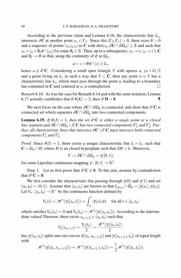
50 J.-F. BABADJIAN, G.A. FRANCFORT
According to the previous claim and Lemma 6.16, the characteristic line Lxn
intersects ∂C at another point yn ∈ Γ2. Since dist (Γ2,Γ1) > 0, there exist δ > 0and a sequence of points (zn)n∈N in C with dist(zn,∂C∩ ∂Ωp) ≥ δ and such thatxn = zn+θnσ⊥(zn) for some θn ∈R. Then, up to a subsequence, yn → y, zn → z∈Cand θn → θ so that, using the continuity of σ in Ωp,
a = z+θσ⊥(z) ∈ Lz,
hence a 6∈ ∂ cC. Considering a small open triangle T with apexes a, (a+ b)/2and a point living on Lz in such a way that T ⊂ C, then any point w ∈ T has acharacteristic line Lw which must pass through the point a, leading to a boundaryfan contained in C and centered at a, a contradiction.
Remark 6.18. As was the case for Remark 6.14 and with the same notation, Lemma6.17 actually establishes that if #(K) = 2, then ∂ cD = /0. 
We next focus on the case where ∂C∩∂Ωp is connected, and show that ∂ cC isconnected set which separates ∂C∩∂Ωp into two connected components.
Lemma 6.19. If #(J) = 1, then the set ∂ cC is either a single point or a closedline segment and ∂C∩∂Ωp \∂ cC has two connected components Γ′
1 and Γ′2. Fur-
ther, all characteristic lines that intersect ∂C\∂ cC must intersect both connectedcomponents Γ′
1 and Γ′2.
Proof. Since #(I) = 1, there exists a unique characteristic line L = L1 such thatC = Ωp ∩H, where H is an closed hyperplane such that ∂H = L. Moreover,
Γ := ∂C∩∂Ωp = γ([0,1])
for some Lipschitz continuous mapping γ : [0,1]→ R2.
Step 1. Let us first prove that ∂ cC 6= /0. To this aim, assume by contradictionthat ∂ cC = /0.
We first consider the characteristic line passing through γ(0) and γ(1) and set(s0, t0) = (0,1). Assume that (sn, tn) are known so that Lγ(sn)∩Ωp = [γ(sn),γ(tn)].Let Vn : [sn, tn]→ R+ be the continuous function defined by
Vn(t) = H 1(γ([sn, t])) =ˆ t
sn
|γ(s)|ds for all t ∈ [sn, tn]
which satisfies Vn(sn) = 0 and Vn(tn) = H 1(γ([sn, tn])). According to the interme-diate valued Theorem, there exists sn+1/2 ∈ (sn, tn) such that
Vn(sn+1/2) =Vn(tn)
2=
H 1(γ([sn, tn])2
,
hus γ([sn, tn]) splits into two curves γ([sn,sn+1/2]) and γ([sn+1/2, tn]) of equal lengthwith
H 1(γ([sn,sn+1/2])) = H 1(γ([sn+1/2, tn])) =12H 1(γ([sn, tn])).

CONTINUITY EQUATION IN HENCKY PLASTICITY 51
Since Ωp is convex, the resulting triangle Tn with vertices γ(sn), γ(tn) and γ(sn+1/2)
satisfies Tn ⊂ Ωp. Moreover, [γ(sn),γ(sn+1/2)]∪ [γ(tn),γ(sn+1/2)] 6⊂ ∂C, otherwiseit would also be lying in ∂C∩∂Ωp because that latter set has only one connectedcomponent by assumption. Then the characteristic line passing through γ(sn+1/2)would necessarily intersect the open segment ]γ(sn),γ(tn)[⊂ Lγ(sn)∩Ωp, which isimpossible by Proposition 5.5. We then define tn+1/2 such that γ(tn+1/2) is theother intersection point of Lγ(sn+1/2) with ∂Ωp. Note that tn+1/2 ∈ (sn, tn) oth-erwise γ(sn) (resp. γ(tn)) would form a boundary fan contained in C. Then ifsn+1/2 < tn+1/2, we define (sn+1, tn+1) := (sn+1/2, tn+1/2), while if sn+1/2 > tn+1/2,we define (sn+1, tn+1) := (tn+1/2,sn+1/2) (see Figure 6.10). The sequence (sn)n∈Nis increasing while (tn)n∈N is decreasing with 0 < sn < sn+1 < tn+1 < tn < 1 for alln ∈ N. Therefore, sn → s and tn → t for some 0 < s ≤ t < 1, and the line segment[sn, tn] converges in the sense of Hausdorff to [s, t]. Since
|γ(tn+1)− γ(sn+1)| ≤ H 1(γ([sn+1, tn+1]))≤ H 1([γ(sn+1/2, tn])
= H 1(γ([sn,sn+1/2])) =H 1(γ([sn, tn])
2≤ H 1(γ([0,1])
2n+1 → 0,
we deduce that γ(s) = γ(t) =: x. Since x 6∈ ∂ cC (because ∂ cC is empty), it lieson a characteristic line Lx which must intersect [γ(sn),γ(tn)], a contradiction withProposition 5.5.
Lγ(sn)
•γ(tn)
•γ(sn)
• γ(sn+1/2) = γ(sn+1)
Lγ(sn+1)
•γ(tn+1)
Γ
L
C
•γ(1)
• γ(0)
FIGURE 6.10. Construction of the sequences (sn)n∈N and (tn)n∈N
Step 2. Assume now that ∂ cC is not connected and consider two distinct con-nected components S and S′ with
t0 := inft ∈ [0,1] : γ(t) ∈ S′> sups ∈ [0,1] : γ(s) ∈ S=: s0.
Then there exists s ∈ [s0, t0] such that x := γ(s) /∈ ∂ cC. Consider the characteristicline Lx passing through x. It must intersect Γ at some other point x′ which cannotcoincide with γ(0) or γ(1), otherwise it would form with L a boundary fan con-tained in C with apex at one of these points. Let H be the closed half-plane withLx as boundary containing both γ(0) and γ(1). Then the region D := C∩H would

52 J.-F. BABADJIAN, G.A. FRANCFORT
be a convex relatively closed subset of Ωp such that, on the one hand, its boundarycontains two characteristic lines L and Lx, and, on the other hand, ∂D∩ ∂Ωp hastwo connected components. Since one of S or S′ is contained in ∂ cD, ∂ cD 6= /0, acontradiction according to Remark 6.18. So ∂ cC is connected and ∂C∩∂Ωp \∂ cChas two connected components Γ′
1 and Γ′2.
Step 3. If ∂ cC is not reduced to a point, it must contain γ((s′, t ′)) for some0 < s′ < t ′ < 1 so that its relative interior in ∂C, denoted by (∂ cC), is not empty.Then, any point x ∈ (∂ cC) is not an accumulation point of (∂C∩ ∂Ωp) \ ∂ cCso that Proposition 6.8-(ii) ensures that x ∈ ]ax,bx[⊂ ∂ cC for some maximal opensegment ]ax,bx[ containing x. If ]ax,bx[ 6= (∂ cC), then ax is not an accumulationof (∂C∩ ∂Ωp) \ ∂ cC, and a new application of Proposition 6.8-(ii) shows that axis contained in another open segment S ⊂ ∂ cC. Then, ]ax,bx[ and S, being on theLipschitz boundary ∂C∩∂Ω, must be aligned so that ]ax,bx[∪S ⊂ ∂ cC is an openline segment containing x which is strictly larger that ]ax,bx[, a contradiction to themaximality of ]ax,bx[. Therefore we must have that ]ax,bx[= (∂ cC), which showsthat ∂ cC is a segment. If ax 6∈ ∂ cC, then there exists z ∈ C such that ax ∈ Lz andax would be the apex of a boundary fan contained in C by an argument identicalto that used at the end of Case II in the proof of Lemma 6.17. Therefore ax ∈ ∂ cCand the same argument shows that bx ∈ ∂ cC. This proves that ∂ cC is a closed linesegment.
Step 4. Assume that there is z ∈ C such that the characteristic line Lz intersectssay Γ′
1 at two distinct points γ(s) and γ(t) ∈ Γ′1. But then the same construction
as in Step 1 would establish the existence of some s ∈ [s, t] such that γ(s) ∈ ∂ cC∩Γ′
1, which is impossible since Γ′1 ⊂ ∂C \ ∂ cC. Alternatively, the closed convex
connected subdomain D := H ∩C of C, where H is the closed half plane withboundary Lz containing ∂ cC, would be such that, in the notation of Remark 6.14,#(K) = 2 while ∂ cD = ∂ cC 6= /0 and Remark 6.18 would lead to a contradiction.Thus all characteristic lines that intersect Γ′
1 must intersect Γ′2 as well.
Remark 6.20. Remark that in Lemma 6.19, for any x ∈ Γ′1, y ∈ Γ′
2, the line segment[x,y] 6⊂ ∂C∩ ∂Ωp. In other words, the boundary ∂C∩ ∂Ωp cannot be flat around∂ cC. Assuming otherwise, consider the Lipschitz parameterization γ of ∂C andassume, for example, that x = γ(s), y = γ(t) with s < t. Take Lx (resp. Ly) be theassociated characteristic lines. Then, Lx must intersect Γ′
2 at γ(t ′) with t ′ > t whileLy must intersect Γ′
1 at γ(s′) with s′ < s. But then, Lx and Ly must intersect in C,which is impossible by Proposition 5.5. 
Remark 6.21. Theorem 6.11 can be rephrased as follows: the non-characteristicexterior boundary ∂C∩∂Ωp \∂ cC has always exactly two connected components,denoted hereafter by Γ1 and Γ2 and all characteristic lines that intersect ∂C mustintersect both Γ1 and Γ2. 

CONTINUITY EQUATION IN HENCKY PLASTICITY 53
The particular geometrical structure of the connected components of C allowsone to improve the continuity of the Cauchy stress σ up to the (non characteristic)boundary.
Theorem 6.22. Let C be a connected component of C with nonempty interior.Then σ is continuous in C\∂ cC.
Proof. We already know that σ is locally Lipschitz continuous on C. It thus re-mains to prove that σ is continuous on ∂C∩ ∂Ωp \ ∂ cC. According to Theorem6.11 and Remark 6.21, we know that ∂C∩ ∂Ωp \ ∂ cC has two connected compo-nents Γ1 and Γ2.
Let x ∈ ∂C∩∂Ωp \∂ cC and (xn)n∈N be a sequence in C\∂ cC such that xn → x.Without loss of generality, we can assume that x ∈ Γ1. Since by Theorem 6.11 Lxn
must intersect both Γ1 and Γ2, there exists an ∈ Lxn ∩Γ1 and bn ∈ Lxn ∩Γ2 which,up to a subsequence, satisfy an → a ∈ Γ1 and bn → b ∈ Γ2. As a consequence, theclosed segment Sn := Lxn ∩Ωp converges in the sense of Hausdorff to the segmentS = [a,b] with x = a.
Case I: Assume first that there exists δ > 0 such that for all n ∈ N,
maxz∈Sn
dist(z,∂C∩∂Ωp)≥ δ ,
then there exists zn ∈ Sn such that dist(zn,∂C∩∂Ωp)≥ δ and, up to a subsequence,zn → z for some z ∈ S with dist(z,∂C∩ ∂Ωp) ≥ δ . Since xn ∈ Lzn , there existsθn ∈ R such that
xn = zn +θnσ⊥(zn).
Note that, up to a further subsequence, θn → θ ∈ R and thus, by continuity of σ
in Ωp, we have x = z+ θσ⊥(z) which ensures that x ∈ Lz. Thus, using that σ isconstant along characteristics and, once again, the continuity of σ in Ωp, we getthat
σ(xn) = σ(zn)→ σ(z) = σ(x).
Case II: Assume next that, up to a subsequence
maxz∈Sn
dist(z,∂C∩∂Ωp)→ 0.
By Hausdorff convergence, for all z ∈ S, there exists a sequence (zn)n∈N with zn ∈Sn and zn → z. Thus, dist(zn,∂C∩ ∂Ωp) → 0 which ensures that S ⊂ ∂C∩∂Ωp.Then S = [a,b] = [x,b] is a line segment contained in ∂C∩ ∂Ωp which contains∂ cC. Further, ∂ cC = [c,d] for some points c,d ∈ ∂C∩ ∂Ωp with c ∈ Γ1, d ∈ Γ2and maybe c= d. Since x /∈ ∂ cC, x= a 6= c, [a,c[∩∂ cC= /0, and there exists a pointx′ ∈ [a,c[ such that x′ /∈ ∂ cC. But then, the characteristic line segment Lx′∩Ωp mustintersect Sn since Sn Hausdorff-converges to [a,b], which is impossible accordingto Proposition 5.5. Thus, this second case never occurs.

54 J.-F. BABADJIAN, G.A. FRANCFORT
The following result is analogous to Proposition 6.3. It gives a uniqueness resultfor the displacement in some portion of C whose boundary intersects the boundaryof the domain Ω.
Proposition 6.23. Let C be a connected component of C with nonempty interior.Extend u by w outside Ω. Then, u+ = u− H 1-a.e. on ∂C∩ ∂Ωp \ ∂ cC and, inparticular, u = w H 1-a.e. on ∂C∩∂Ωp ∩∂Ω\∂ cC.
Proof. In the current setting, ∂C∩ ∂Ωp \ ∂ cC has two connected components Γ1and Γ2 which are open in the relative topology of ∂Ωp and Lipschitz. According toRemark 3.1, σ ·ν =±1 H 1-a.e. on ∂C∩∂Ωp ∩ Ju \∂ cC. Theorem 6.22 ensuresthat σ is continuous in C \ ∂ cC. We thus deduce that σ · ν coincides H 1-a.e.with the usual scalar product of σ and ν on ∂C∩∂Ωp \∂ cC. Therefore, ν =±σ
H 1-a.e. on ∂C∩∂Ωp ∩ Ju \∂ cC.Assume that H 1(∂C∩ ∂Ωp ∩ Ju \ ∂ cC) > 0, we can find a point x0 ∈ ∂C∩
∂Ωp ∩ Ju \ ∂ cC such that, up to a change of sign, ν(x0) = σ(x0). It thus followsthat Lx0 is tangent to C at x0 which is in contradiction with the fact that x0 6∈ ∂ cC.Therefore, H 1(∂C∩ ∂Ωp ∩ Ju \ ∂ cC) = 0 and thus, u+ = u− H 1-a.e. on ∂C∩∂Ωp \∂ cC.
Using the Dirichlet boundary condition, we get that u = w H 1-a.e. on ∂C∩∂Ωp ∩∂Ω\∂ cC.
Remark 6.24. If Ω was a convex domain and if σ was such that |σ | ≡ 1 in Ω, then,Ω = Ωp would be the disjoint union of characteristic lines Lxλ
(see Proposition6.5), of countably many boundary fans Fzi , and of countably many connected com-ponents C j (with non empty interior) such that every point in ∂C j ∩∂Ω\ ∂ cC j istraversed by a characteristic line (see Theorem 6.11). Since all characteristic linescut ∂Ω into two distinct points by convexity of Ω, then u is entirely determinedby w in each fan Fz j according Proposition 6.3. Similarly, by virtue of Proposition6.23, u(x) = w(x) for H 1-a.e. x ∈ ∂C j ∩∂Ω\∂ cC j and, finally, by Theorem 5.6,u is constant along H 1-a.e. associated characteristic line Lx.
Since it is generically not so that the values of w at both points of Lx∩∂Ω shouldmatch, this situation is not possible. Therefore, in the scalar case with a genericDirichlet boundary condition over the entire boundary, a convex body cannot beentirely plastified unless it is made only of boundary fans.
However, as seen in the example in the introduction, the situation is different inthe case of mixed boundary conditions. 
6.3 MiscellaneaExterior fans
In contrast with the case of boundary fans, it might happen that two characteris-tic lines which intersect outside Ωp will not generate an exterior fan. In particular,
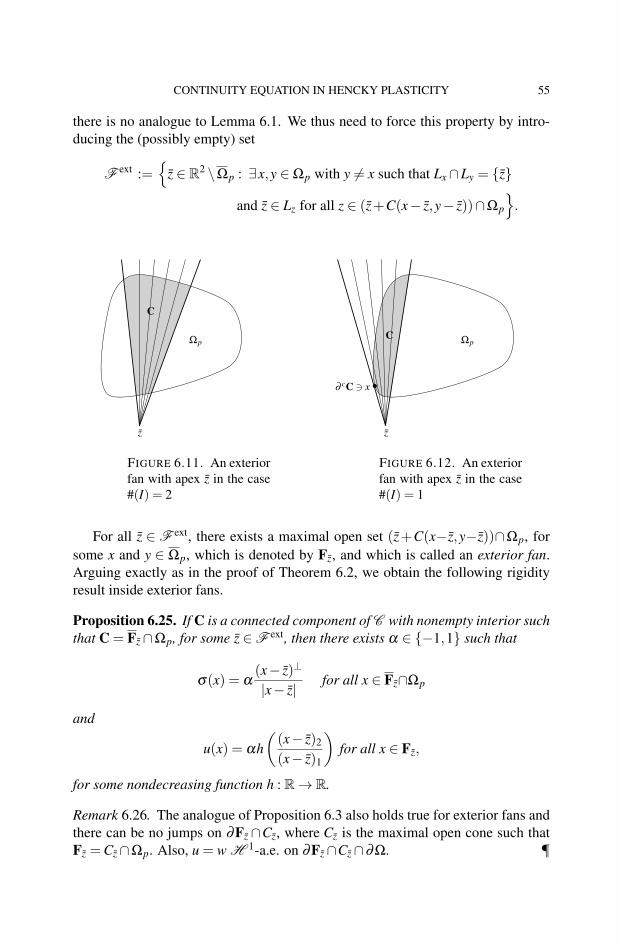
CONTINUITY EQUATION IN HENCKY PLASTICITY 55
there is no analogue to Lemma 6.1. We thus need to force this property by intro-ducing the (possibly empty) set
F ext :=
z ∈ R2 \Ωp : ∃x,y ∈ Ωp with y 6= x such that Lx ∩Ly = z
and z ∈ Lz for all z ∈ (z+C(x− z,y− z))∩Ωp
.
C
Ωp
z
FIGURE 6.11. An exteriorfan with apex z in the case#(I) = 2
•∂ cC 3 x
CΩp
z
FIGURE 6.12. An exteriorfan with apex z in the case#(I) = 1
For all z ∈ F ext, there exists a maximal open set (z+C(x−z,y−z))∩Ωp, forsome x and y ∈ Ωp, which is denoted by Fz, and which is called an exterior fan.Arguing exactly as in the proof of Theorem 6.2, we obtain the following rigidityresult inside exterior fans.
Proposition 6.25. If C is a connected component of C with nonempty interior suchthat C = Fz ∩Ωp, for some z ∈ F ext, then there exists α ∈ −1,1 such that
σ(x) = α(x− z)⊥
|x− z|for all x ∈ Fz∩Ωp
and
u(x) = αh((x− z)2
(x− z)1
)for all x ∈ Fz,
for some nondecreasing function h : R→ R.
Remark 6.26. The analogue of Proposition 6.3 also holds true for exterior fans andthere can be no jumps on ∂Fz ∩Cz, where Cz is the maximal open cone such thatFz =Cz ∩Ωp. Also, u = w H 1-a.e. on ∂Fz ∩Cz ∩∂Ω. 

56 J.-F. BABADJIAN, G.A. FRANCFORT
Constant zonesConstant zones have a special structure.
Proposition 6.27. If C is a connected component of C with nonempty interior onwhich σ = σ is constant, then u(x) = σ · x+ v(σ · x) for all x ∈ C for some nondecreasing function v, and, if ∂C∩∂Ωp has two connected components, then bothcharacteristic lines L1 and L2 lying on ∂C∩Ωp are parallel to Rσ⊥.
Proof. Assume for simplicity that σ = e1 = (1,0). Addressing the last part of theProposition, if one of both characteristic lines, say L1, lying on ∂C∩Ωp is notparallel to e2 = (0,1), then there exists x ∈ C such that Lx intersects L1 inside Ωpwhich is absurd in view of Proposition 5.5.
Further, with the help of (4.17),
D2|p|= div(σ⊥(L 2 + |p|)) = 0 in D ′(C),
which means that |p| is independent of x2. As a consequence, |p| = πx1 ⊗L 1x2
forsome nonnegative measure π = πx1 ∈ M (R), i.e.,ˆ
Cϕ d|p|=
ˆC
ϕ(x1,x2)dπ(x1)dx2 for all ϕ ∈ Cc(C).
This implies, in view of (4.17), that Du = e1(1+πx1 ⊗L 1x2) on C. Hence u(x) =
x1 + v(x1) for a.e. x ∈ C for some v ∈ BV (R) with Dv = π ≥ 0.
CΩp
FIGURE 6.13. A constantzone in the case #(I) = 2
C Ωp
•∂ cC 3 x
FIGURE 6.14. A constantzone in the case #(I) = 1
An example of a non-fan, non-constant structureAssume that a connected component C of Ωp is such that C ⊂ (0,R)2, for some
R > 0, and that the characteristic lines are given by the one-parameter family
Lt =(x,y) ∈ R2 : y =
xt− t, t > 0.

CONTINUITY EQUATION IN HENCKY PLASTICITY 57
y
x
CΩp
FIGURE 6.15. An example of a non-fan, non-constant structure
Note that this family of lines does not intersect at a single point so that it does notdefine an exterior fan (see Figure 6.15). However, we are going to construct anexample of smooth solutions (u,σ , p) of
divσ = 0, |σ |= 1 in C,
∇u = σ + p, p = σ |p| in C,
such that u and σ are constant along Lt ∩C for all t > 0. Doing so, we will havesatisfied all equations (3.2) on C, ignoring the boundary condition on ∂Ω and re-calling Remark 4.5.
Let us start by constructing a (unique) stress σ : C → R2. Indeed, since σ(x,y)must be an unimodular vector orthogonal to Lt at (x,y = x
t − t), then
σ(x,y) =1√
1+ t2
(−1t
)with t =
−y+√
y2 +4x2
,
hence
σ(x,y) :=2√
4+(√
y2 +4x− y)2
(−1√
y2+4x−y2
).
Then σ ∈ C ∞(C;R2) and, by construction, |σ | = 1 in C. Further a lengthy com-putation would show that divσ = 0 in C.
We now construct the displacement u : C → R as u(x,y) := f (√
y2 +4x −y) for all (x,y) ∈ C, for some smooth decreasing function f : R+ → R such that
(6.8) f ′(t)≤− R+ t√4+ t2
for all t > 0.
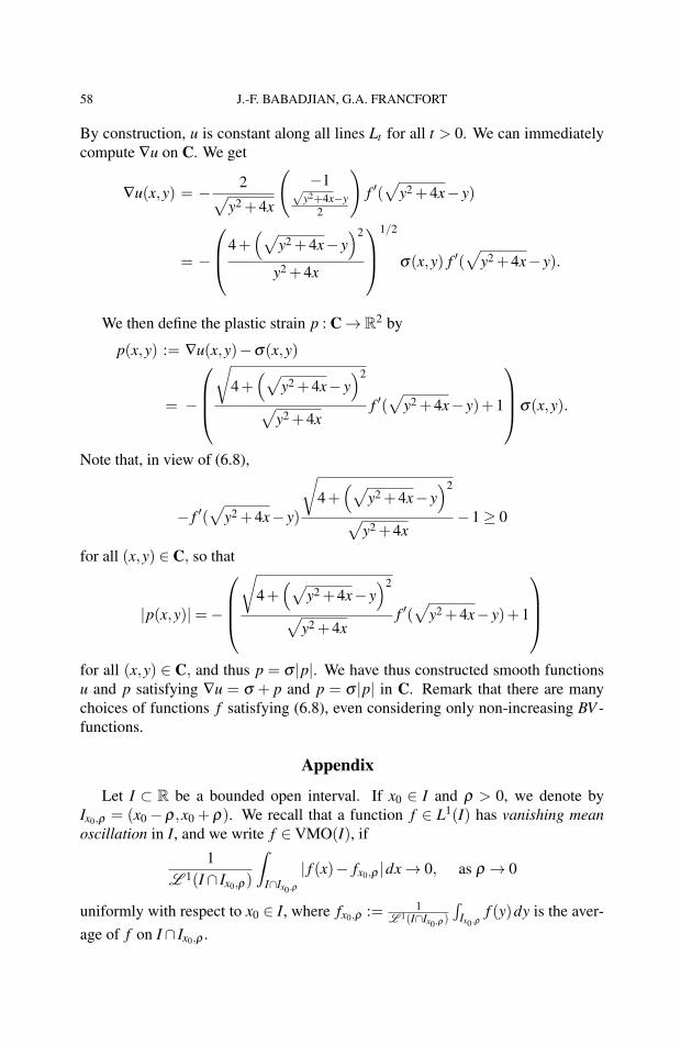
58 J.-F. BABADJIAN, G.A. FRANCFORT
By construction, u is constant along all lines Lt for all t > 0. We can immediatelycompute ∇u on C. We get
∇u(x,y) = − 2√y2 +4x
(−1√
y2+4x−y2
)f ′(√
y2 +4x− y)
= −
4+(√
y2 +4x− y)2
y2 +4x
1/2
σ(x,y) f ′(√
y2 +4x− y).
We then define the plastic strain p : C → R2 by
p(x,y) := ∇u(x,y)−σ(x,y)
= −
√
4+(√
y2 +4x− y)2
√y2 +4x
f ′(√
y2 +4x− y)+1
σ(x,y).
Note that, in view of (6.8),
− f ′(√
y2 +4x− y)
√4+(√
y2 +4x− y)2
√y2 +4x
−1 ≥ 0
for all (x,y) ∈ C, so that
|p(x,y)|=−
√
4+(√
y2 +4x− y)2
√y2 +4x
f ′(√
y2 +4x− y)+1
for all (x,y) ∈ C, and thus p = σ |p|. We have thus constructed smooth functionsu and p satisfying ∇u = σ + p and p = σ |p| in C. Remark that there are manychoices of functions f satisfying (6.8), even considering only non-increasing BV -functions.
Appendix
Let I ⊂ R be a bounded open interval. If x0 ∈ I and ρ > 0, we denote byIx0,ρ = (x0 − ρ,x0 + ρ). We recall that a function f ∈ L1(I) has vanishing meanoscillation in I, and we write f ∈ VMO(I), if
1L 1(I ∩ Ix0,ρ)
ˆI∩Ix0 ,ρ
| f (x)− fx0,ρ |dx → 0, as ρ → 0
uniformly with respect to x0 ∈ I, where fx0,ρ := 1L 1(I∩Ix0 ,ρ )
´Ix0 ,ρ
f (y)dy is the aver-age of f on I ∩ Ix0,ρ .

CONTINUITY EQUATION IN HENCKY PLASTICITY 59
We first show a (well known) result (see [13, Example 2]).
Lemma A.1. If f ∈ H1/2(I), then f ∈ VMO(I).
Proof. Since f ∈ H1/2(I), then by definition¨I×I
| f (x)− f (y)|2
|x− y|2dxdy <+∞.
Therefore, by absolute continuity of the integral, for each ε > 0 there exists δ > 0such that for every Lebesgue measurable set A ⊂ I × I with L 2(A)≤ δ , then¨
A
| f (x)− f (y)|2
|x− y|2dxdy ≤ ε
2.
Let x0 ∈ I and ρ ≤√
δ/2 so that L 2(Ix0,ρ × Ix0,ρ) = 4ρ2 ≤ δ . According to thetriangle and Cauchy-Schwarz inequalities, we have
1L 1(I ∩ Ix0,ρ)
ˆI∩Ix0 ,ρ
| f (x)− fx0,ρ |dx
≤ 1L 1(I ∩ Ix0,ρ)
2
¨(I∩Ix0 ,ρ )
2| f (x)− f (y)|dxdy
≤
(1
L 1(I ∩ Ix0,ρ)2
¨(I∩Ix0 ,ρ )
2| f (x)− f (y)|2 dxdy
)1/2
.
If x and y ∈ I ∩ Ix0,ρ , then, |x− y| ≤ L 1(I ∩ Ix0,ρ), hence
1L 1(I ∩ Ix0,ρ)
ˆIx0 ,ρ
| f − fx0,ρ |dx
≤
(¨(I∩Ix0 ,ρ )
2
| f (x)− f (y)|2
|x− y|2dxdy
)1/2
≤ ε,
which proves that f ∈ VMO(I).
We now show that a characteristic function which belongs to H1/2(I) must beconstant.
Lemma A.2. Let χ = 1A for some Lebesgue measurable set A ⊂ I. If χ ∈ H1/2(I)then either L 1(A) = 0 or L 1(I \A) = 0.
Proof. For L 1-a.e. y ∈ I ∩ Ix,ρ we have that dist(χx,ρ ,0,1) ≤ |χx,ρ − χ(y)|.Lemma A.1 implies that χ ∈ VMO(I). Therefore, integrating over I ∩ Ix,ρ , weget
dist(χx,ρ ,0,1)≤ 1L 1(I ∩ Ix,ρ)
ˆI∩Ix,ρ
|χ −χx,ρ |dy → 0

60 J.-F. BABADJIAN, G.A. FRANCFORT
as ρ → 0, uniformly with respect to x ∈ I. In particular, there exists ρ0 > 0 suchthat dist(χx,ρ ,0,1) < 1/3 for all 0 < ρ < ρ0 and all x ∈ I. Let ρ < ρ0. Sincethe function x ∈ I 7→ χx,ρ is continuous, then, either χx,ρ ≤ 1/3 for all x ∈ I, orχx,ρ ≥ 2/3 for all x ∈ I. But, since χx,ρ → χ(x) as ρ → 0 for every Lebesgue pointx ∈ I of χ , then, either χ = 0 a.e. in I, or χ = 1 a.e. in I.
We next prove that a piecewise constant function on a Lipschitz graph cannotbelong to H1/2.
Lemma A.3. Let Γ = Γ−∪Γ+ where Γ± are segments in R2 such that Γ+∩Γ
− isa single point. Let f : Γ → R be such that f = α on Γ− and f = β on Γ+ whereα 6= β . Then f 6∈ H1/2(Γ).
Proof. Without loss of generality, we suppose that Γ ⊃ (x1,x2) ∈R2 : −L < x1 <L, x2 = a|x1| where L > 0, a > 0, Γ− = (x1,x2)∈R2 : −L < x1 < 0, x2 =−ax1and Γ+ = (x1,x2) ∈ R2 : 0 < x1 < L, x2 = ax1. Let us show that
¨Γ×Γ
| f (x)− f (y)|2
|x− y|2dH 1(x)dH 1(y) = +∞.
Indeed, using the definition of a curvilinear integral and a change of variables¨
Γ×Γ
| f (x)− f (y)|2
|x− y|2dH 1(x)dH 1(y)
= 2|α −β |2¨
Γ−×Γ+
dH 1(x)dH 1(y)|x− y|2
= 2(1+a2)|α −β |2¨
(−L,0)×(0,L)
dx1 dy1
(x1 − y1)2 +a2(x1 + y1)2
= 2(1+a2)|α −β |2¨
(0,L)2
dsdt(s+ t)2 +a2(s− t)2 .
Since (s+ t)2 +a2(s− t)2 ≤ 2(1+a2)(s2 + t2), we deduce that¨
Γ×Γ
| f (x)− f (y)|2
|x− y|2dH 1(x)dH 1(y) ≥ |α −β |2
¨(0,L)2
dsdts2 + t2
≥ |α −β |2¨
DL
dsdts2 + t2 ,
where DL := (0,L)2 ∩BL(0) is the right upper quarter of a disk of radius L. Usinga change of variables in polar coordinates, we get that
¨DL
dsdts2 + t2 =
π
2
ˆ L
0
drr
=+∞,
which completes the proof of the result.

CONTINUITY EQUATION IN HENCKY PLASTICITY 61
Acknowledgment. This research was supported by the National Science Fundation Grants DMS-
1615839 and DMS/DMREF-1922371 and was completed in part while the first author was visiting the Courant
Institute in April 2019 with the support of Grant DMS-1615839. The first author’s research was also partially
supported by a public grant as part of the Investissement d’avenir project, reference ANR-11-LABX-0056-LMH,
LabEx LMH. The second author also wishes to thank the Flatiron Institute of the Simons Foundation for its
hospitality.
Bibliography[1] Ambrosio, L. Transport equation and Cauchy problem for BV vector fields. Inventiones Math.
158 (2004), 227–260.[2] Ambrosio, L., Fusco, N. and Pallara, D. Functions of Bounded Variation and Free Discontinuity
Problems. Oxford University Press, Oxford, 2000.[3] Anzellotti, G. Pairings between measures and bounded functions and compensated compact-
ness. Ann. Mat. Pura Appl. 135(1983), no. 4, 293–318.[4] Anzellotti, G. On the existence of the rates of stress and displacements for Prandtl-Reuss plas-
ticity. Quart. Appl. Math. 41 (1984), 181–208.[5] Anzellotti, G. On the extremal stress and displacement in Hencky plasticity. Duke Math. J.
51(1984), no.1, 133–147 .[6] Anzellotti, G. and Luckhaus, S. Dynamical evolution of elasto-perfectly plastic bodies. Appl.
Math. Optim. 15 (1987), no. 2, 121–140.[7] Babadjian, J.-F. and Francfort, G. A. A note on the derivation of rigid-plastic models. Nonlinear
Differential Equations Appl. 23 (2016), no. 3, 23–37.[8] Babadjian, J.-F. and Mifsud, C. Hyperbolic structure for a simplified model of dynamical per-
fect plasticity. Arch. Rational Mech. Anal. 223 (2017), no. 2, 761–815.[9] Babadjian, J.-F. and Mora, M. G. Stress regularity in quasi-static perfect plasticity with a pres-
sure dependent yield criterion. J. Differential Eq. 264 (2018), no. 8, 5109–5151.[10] Ball, J.M. Convexity conditions and existence theorems in nonlinear elasticity. Arch. Rat. Mech.
Anal. 63 (1977), no. 4, 337–403.[11] Bensoussan, A. Frehse, J. Asymptotic behaviour of Norton-Hoff’s law in plasticity theory and
H1 regularity. Boundary value problems for partial differential equations and applications,RMA Res. Notes Appl. Math. 29 (1993), 3–25.
[12] Bochard, P. and Pegon, P. Kinetic selection principle for curl-free vector fields of unit norm.Comm. Partial Diff. Eq. 42 (2017), 1375–1402.
[13] Brezis, H. and Nirenberg, L. Degree theory and BMO. I. Compact manifolds without bound-aries. Selecta Math. (N.S.) 1 (1995), no. 2,197–263.
[14] Chen, G.-Q. and Frid, H. Divergence-measure fields and hyperbolic conservation laws. Arch.Ration. Mech. Anal. 147 (1999), no. 2. 89–118.
[15] G. Crippa, G. and De Lellis, C. Estimates for transport equations and regularity of the DiPerna-Lions flow. J. Reine Angew. Math. 616 (2008), 15–46.
[16] Dal Maso, G.,De Simone, A. and Mora, M.G. Quasistatic evolution problems for linearly elasticperfectly plastic materials. Arch. Rat. Mech. Anal. 181 (2006), no. 2, 237–291.
[17] David, G. Singular sets of minimizers for the Mumford-Shah functional, Progress in Mathemat-ics (Volume 233), Birkhaüser Verlag, Basel, 2005.
[18] De Lellis, C. and Székelyhidi Jr., L. The Euler equations as a differential inclusion. AnnalsMath. 170 (2009), no. 3, 1417–1436.
[19] Demyanov, A. Regularity of stresses in Prandtl-Reuss perfect plasticity. Calc. Var. PartialDifferential Equations 34 (2009), no. 1, 23–72.

62 J.-F. BABADJIAN, G.A. FRANCFORT
[20] De Simone, A., Kohn, R. V., Müller, S. and Otto, F. A compactness result in the gradient theoryof phase transitions. Proc. Roy. Soc. Edinburgh 131 (2001), 833–844.
[21] Di Perna, R. J. and Lions P. L. Ordinary differential equations, transport theory and Sobolevspaces. Invent. Math. 98 (1989), 511–547.
[22] Evans, L.C. and Gariepy R.F. Measure Theory and Fine Properties of Functions. CRC Press,Boca Raton, 1992.
[23] Fonseca, I. and Gangbo, W. Degree theory in analysis and applications, Oxford lecture seriesin mathematics and its applications 2. Clarendon Press, Oxford, 1995.
[24] Francfort, G. A. and Giacomini, A. Small-strain heterogeneous elastoplasticity revisited.Comm. Pure Appl. Math. 65 (2012), no. 9, 1185–1241.
[25] Francfort, G. A., Giacomini, A. and Marigo, J.-J. The taming of plastic slips in von Miseselasto-plasticity. Interfaces Free Bound. 17 (2015), 497–516.
[26] Francfort, G. A., Giacomini, A. and Marigo, J.-J. A case study for uniqueness of elasto-plasticevolutions: The bi-axial test. J. Math. Pures Appl. 105 (2016), 198–227.
[27] Francfort, G. A., Giacomini, A. and Marigo, J.-J. The elasto-plastic exquisite corpse: A Suquetlegacy. J. Mech. Phys. Sol. 97 (2016), 125–139.
[28] Henrot, A. and Pierre, M. Shape variation and optimization. A geometrical analysis, EMSTracts in Mathematics, 28. European Mathematical Society (EMS), Zürich, 2018.
[29] Ignat, R. Two-dimensional unit-length vector fields of vanishing divergence, J. Funct. Anal.262 (2012), no. 8, 3465–3494.
[30] Jabin, P.-E. , Otto, F. and Perthame B. Line-energy Ginzburg-Landau models: zero-energystates. Ann. Sc. Norm. Super. Pisa Cl. Sci. (5) 1 (2002), no. 1, 187–202.
[31] Kohn, R.V. and Temam R. Dual spaces of stresses and strains, with applications to Henckyplasticity. Appl. Math. Optim. 10 (1983), no. 1, 1–35.
[32] J. Lubliner, J. Plasticity Theory. Macmillan Publishing Company, New York, 1990.[33] Mielke A. Evolution of rate-independent systems. Evolutionary equations. Vol. II, Handb. Dif-
fer. Equ., 461–559. Elsevier/North-Holland, Amsterdam, 2005.[34] Mora, M.G. Relaxation of the Hencky model in perfect plasticity. J. Math. Pures Appl. 9-106
(2016), no. 4, 725–743.[35] Murat, F. and Trombetti, C. A chain rule formula for the composition of a vector-valued func-
tion by a piecewise smooth function Boll. U. Mat. Ital., Serie 8 6-B (2003), no. 3, 581–595.[36] Seregin, G.A. On the differentiability of extremals of variational problems of the mechan-
ics of ideally elastoplastic media, (Russian). Differentsial’nye Uravneniya 23 (1987), no. 11,1981–1991.
[37] Suquet, P.-M. Sur les équations de la plasticité: existence et régularité des solutions J. Mé-canique 20 (1981), no. 1, 3–39.
[38] Temam, R. Problèmes Mathématiques en Plasticité. Gauthier-Villars, Paris, 1983.