
Multibody Analysis of Solar Array Deployment using ...
180
UNIVERSITÀ DI PISA Facoltà di Ingegneria Corso di Laurea in Ingegneria Aerospaziale Tesi di Laurea Multibody Analysis of Solar Array Deployment using Flexible Bodies Anno Accademico 2006-2007 Relatori Prof. G. Mengali Prof. A. Salvetti Dr. B. Specht Candidato: Luca Bagnoli
Transcript of Multibody Analysis of Solar Array Deployment using ...
UNIVERSITÀ DI PISA
Facoltà di Ingegneria Corso di Laurea in Ingegneria Aerospaziale
Tesi di Laurea
Multibody Analysis of Solar Array
Deployment using Flexible Bodies
Anno Accademico 2006-2007
Relatori
Prof. G. Mengali
Prof. A. Salvetti
Dr. B. Specht
Candidato:
Luca Bagnoli

„man muss noch Chaos in sich haben,
um einen tanzenden Stern gebären zu können“
Friedrich Nietzsche

Abstract
The solar panels represent the main device for collecting and converting solar energy into electrical energy and they are widely used in space missions supplying the energy necessary for both spacecrafts and payloads. To optimize the sun exposed surface the panels are usually organized in wings configurations, that, stored during the launch, deploy in the space at the beginning of the operative phase of the satellite. This work of thesis focus on this deployment phase and on the associated dynamic loads. The need of this investigation is connected to the strict requirements on the deployment. Since we want to be sure of the complete deployment in every condition with high margin of safety, the energy stored in the deployment mechanism is quite oversized. This leads to the dynamic loads that we want to estimate. The key topic of the thesis consists in the generation of a flexible multi-body model for solar arrays deployment studies and analysis. The main aim of this model is the verification and validation of a usually pre-existing rigid model used for the conceptual studies of the deployment. In this rigid model, generated directly in ADAMS environment, all the structural stiffness is condensed in a small number of DOF (rotational springs located on the hinge lines). It’s clear that this way of modelling does not cover higher frequency or side dynamics effects. By the introduction of a flexible model we want to investigate these effects and check the right working of the mechanism also in presence of deformation. Optionally, using the flexible model, we can also have a first estimation of stresses and strains due to the dynamics of the deployment. The two main requirements for a flexible model are to be easy to generate and to be compatible with the related rigid model. These two aspects are important to avoid significant impact on the project budget. The flexible bodies are generated using the user friendly interface of PATRAN (avoiding or minimizing manual inputs in NASTRAN) and then importing this flexible bodies in an ADAMS adapted rigid model (avoiding to re-built the flexible model from the beginning). The first chapter of the thesis will show the theoretical background of the NASTRAN-ADAMS interface for the generation of flexible bodies. This theoretical part, even if not strictly necessary for the final-user, is anyway important for the full comprehension of some of the choices that will be adopted. The second chapter will introduce and explain the main characteristics of a solar array rigid model using BEPI COLOMBO MPO solar array and AMOS 3 solar array as examples. The third chapter will focus on the generation of the flexible model using the same two formers examples. In chapter four the results of the two models will be compared and in the fifth chapter the consequent conclusions will be drawn. In last chapter six will be shown other possible fields of application of the flexible body modelling with ADAMS.
ii
I pannelli solari rappresentano il principale sistema per raccogliere e convertire energia solare in energia elettrica e sono largamente utilizzati in missioni spaziali per fornire l’energia necessaria sia al satellite che al suo payload. Per ottimizzare la superficie esposta al sole i pannelli sono spesso organizzati in configurazioni alari che, raccolte durante la fase di lancio, vengono dispiegate nello spazio all’inizio della fase operativa del satellite. Questo lavoro di tesi è focalizzato su questa fase di dispiegamento e sui carichi dinamici ad essa associati. Il bisogno di questa indagine è connesso ai severi requisiti imposti sul dispiegamento. Dato che vogliamo essere sicuri del completo dispiegamento in qualsiasi condizione operativa con un alto margine di sicurezza, l’energia immagazzinata nel sistema di apertura è sovradimensionata. Questo produce i carichi dinamici nella struttura che vogliamo stimare. Il principale obiettivo del presente lavoro di tesi consiste nella generazione di un modello multi-body a corpi flessibili per lo studio e l’analisi del dispiegamento dei pannelli solari. Lo scopo di questo modello sarà quello di verificare e convalidare i risultati di un modello rigido preesistente utilizzato nei primi studi concettuali di dispiegamento. In questo modello rigido, generato direttamente in ambiente ADAMS, la rigidezza strutturale è condensata in un ridotto numero di g.d.l. (molle rotazionali collocate lungo le linee di cerniera). E’ chiaro che questa modellazione non compre quindi effetti di alta frequenza o di dinamiche trasversali. Con l’introduzione del modello flessibile vogliamo investigare questi effetti, controllare il corretto funzionamento del meccanismo anche in presenza di deformazioni ed eventualmente avere una prima stima delle tensioni dovute alla dinamica del dispiegamento. I principali due requisiti del modello flessibile sono la facilità di generazione e la compatibilità con il relativo modello rigido. Questi due aspetti sono di fondamentale importanza per evitare impatti significativi sul budget del progetto. Per ottenere il modello flessibile, i vari corpi che lo compongono sono generati utilizzando l’interfaccia grafica di PATRAN (cercando di evitare e minimizzare gli input diretti nel codice NASTRAN) e quindi importati in un modello rigido adattato in ADAMS (evitando in questo modo di costruire un modello flessibile dall’inizio). Il primo capitolo della tesi riporta la teoria matematica su cui si basa l’interfaccia NASTRAN-ADAMS per la generazione dei corpi flessibili. Questa parte teorica, anche se non strettamente necessaria all’utente finale del modello, è importante per la piena comprensione di alcune delle scelte che verranno adottate. Il secondo capitolo introduce e spiega le principali caratteristiche del modello rigido utilizzando due diverse configurazioni di pannelli solari come esempi, quella del MPO (Mercury Polar Orbiter) di BEPI COLOMBO e quella del satellite di telecomunicazioni AMOS 3. Il terzo capitolo riguarda la generazione del modello flessibile e vengono utilizzate a scopo esplicativo le solite due configurazioni del capitolo precedente. Il capitolo quarto contiene una comparazione tra i due modelli e il quinto le conclusioni che ne emergono. L’ultimo capitolo riporta altre possibili applicazioni per l’utilizzo di modelli flessibili in ADAMS.

Acknowledgement This work of thesis is the result of a six months stage in EADS Astrium GmbH, Mechanical and Thermal analysis & test department, Friedrichshafen, Germany. For this extraordinary and formative experience I’m grateful first of all to my Professor Giovanni Mengali and to Stefano Lucarelli. They made this experience possible and enlarged my horizons, always ready to support and encourage me. For his trust and the opportunity to be part of his team my sincere gratitude goes to Dr. Werner Konrad. This work has not been possible without the patient, the advices and the teachings of my advisor Dr. Bernhard Specht. My warm gratefulness goes to him. His suggestions and his critics were precious for my personal growth and for the right development of this thesis. A particular thanks to Danilo, Domenico, Guenther and Stephen. With them I shared more than a working experience and they represent the piece of Germany I miss more. Many people passed through these university years and all of them contributed in some way to this result. Mentioning them here doesn’t want to be a reward but just a way to make them understand how important they are and how strongly influenced me. My first thought goes to my parents, to my brother and to my whole family. For their support and for supporting me, for their blind trust and their proudness of me that has always made me feel special. It’s rhetorical to say that I would not be here without them… it is not the gratitude and my true love that I owe them but too many times I forgot to express. To Francesca. For all the countless beautiful moments spent together and all the dreams we shared during these years. For being and always having been close. To Gabriele. For his brotherly friendship, his precious support and his contagious order. To my historical friends Adalberto, Andrea, Emanuele, Gabriele, Gigi and Simone. Inseparable adventures and everyday life companions, always present, always ready to remind me not to take myself and life too seriously. To all the other friends that, even if their names can’t be present in these few rows, will always have their place in my thoughts and my memories. Thank you all. I’m sure my happiness is your happiness today, and this my greatest triumph.
iv
Questo lavoro di tesi è il risultato di uno stage di sei mesi presso EADS Astrium GmbH, dipartimento di analisi Termica e Meccanica, Friedrichshafen, Germania. Per questa straordinaria e formativa esperienza sono grato prima di tutto al mio Professore Giovanni Mengali e a Stefano Lucarelli. Loro hanno reso possibile questa esperienza e allargato i miei orizzonti, sempre pronti ad aiutarmi e incoraggiarmi. Per la sua fiducia e l’opportunità di far parte del suo team la mia sincera gratitudine va al Dr. Werner Konrad. Questo lavoro non sarebbe stato possibile senza la pazienza, i consigli e gli insegnamenti del mio advisor Dr. Bernhard Specht. Devo a lui calorosi ringraziamenti. I suoi suggerimenti e le sue critiche sono stati preziosi per la mia crescita personale e per la buona riuscita di questa tesi. Un grazie particolare a Danilo, Domenico, Guenther e Stephen. Con loro ho condiviso più che una esperienza di lavoro e rappresentano la parte della Germania di cui sento maggiormente la mancanza. Molte persone hanno attraversato questi anni universitari e tutte loro hanno contribuito in qualche modo a questo risultato. Menzionarle qui non vuole essere un premo ma solo un modo per far loro capire quanto siano state importanti per me e quanto fortemente mi abbiano influenzato. Il primo pensiero va ai miei genitori, a mio fratello e a tutta la mia famiglia. Per il loro supporto e per l’avermi sopportato, per la loro fiducia e l’orgoglio nei miei confronti che mi ha fatto sempre sentire speciale. E’ retorico dire che non sarei qui senza di loro…non lo è il sincero affetto e la gratitudine che devo loro ma troppe volte ho dimenticato di esprimere. A Francesca. Per gli innumerevoli stupendi momenti passati insieme e per tutti i sogni che abbiamo condiviso in questi anni. Per essere ed essere sempre stata vicina. A Gabriele. Per la sua fraterna amicizia, il suo prezioso supporto e il suo ordine contagioso. Ai mie amici storici Adalberto, Andrea, Emanuele, Gabriele, Gigi e Simone. Inseparabili compagni di avventure e della vita di tutti i giorni, sempre presenti, sempre pronti a ricordarmi di non prendere la vita o me stesso troppo sul serio. A tutti gli altri amici che non possono trovare spazio tra queste poche righe, ma che avranno sempre un posto particolare nei miei ricordi e pensieri. Grazie a tutti voi. Sono sicuro che la mia felicità e anche la vostra oggi, e questa è la mia vittoria più grande.
Luca Bagnoli Pisa, 17 Ottobre 2007

Contents
Abstract............................................................................................................................. i
Aknowledgement............................................................................................................iii
Contents ........................................................................................................................... v
List of Figures................................................................................................................. ix
List of Tables ................................................................................................................xiii
Acronyms...................................................................................................................... xiv
1 Theoretical Background............................................................................................. 1
1.1 The base of the flexible model.............................................................................. 1 1.2 Modal superposition ............................................................................................. 2
1.2.1 Component mode synthesis — The Craig-Bampton method ......................... 3 1.2.2 Mode shape orthonormalization ..................................................................... 6
1.3 Modal flexibility in ADAMS.............................................................................. 10 1.3.1 Flexible marker kinematics........................................................................... 10
1.3.1.1 Position ................................................................................................ 10 1.3.1.2 Velocity................................................................................................ 12 1.3.1.3 Orientation ........................................................................................... 13 1.3.1.4 Angular velocity .................................................................................. 15
1.3.2 Applied loads ................................................................................................ 15 1.3.2.1 Point forces and torques....................................................................... 15
1.3.3 Flexible body equations of motion ............................................................... 17 1.3.3.1 Kinetic energy and the mass matrix..................................................... 18 1.3.3.2 Potential energy and the stiffness matrix............................................. 21 1.3.3.3 Dissipation and the damping matrix .................................................... 22 1.3.3.4 Constraints ........................................................................................... 22 1.3.3.5 Governing differential equation of motion — final form .................... 22
Contents vi
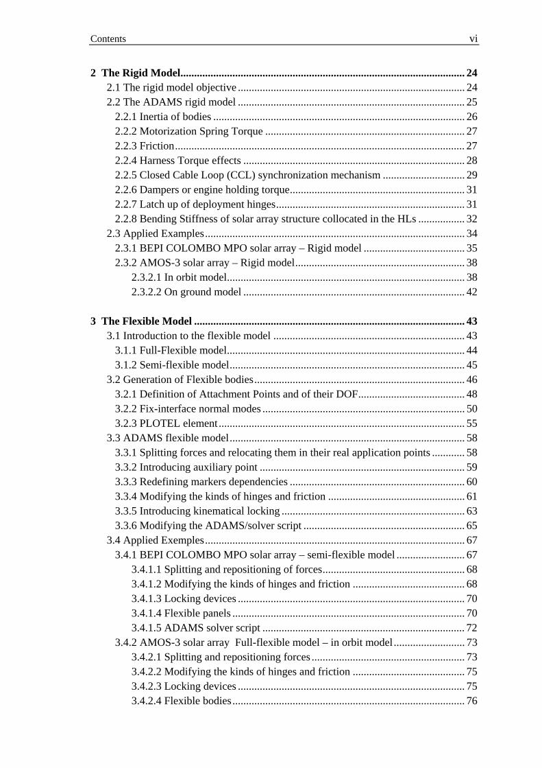
2 The Rigid Model........................................................................................................ 24 2.1 The rigid model objective ................................................................................... 24 2.2 The ADAMS rigid model ................................................................................... 25
2.2.1 Inertia of bodies ............................................................................................ 26 2.2.2 Motorization Spring Torque ......................................................................... 27 2.2.3 Friction.......................................................................................................... 27 2.2.4 Harness Torque effects ................................................................................. 28 2.2.5 Closed Cable Loop (CCL) synchronization mechanism .............................. 29 2.2.6 Dampers or engine holding torque................................................................ 31 2.2.7 Latch up of deployment hinges..................................................................... 31 2.2.8 Bending Stiffness of solar array structure collocated in the HLs ................. 32
2.3 Applied Examples............................................................................................... 34 2.3.1 BEPI COLOMBO MPO solar array – Rigid model ..................................... 35 2.3.2 AMOS-3 solar array – Rigid model.............................................................. 38
2.3.2.1 In orbit model....................................................................................... 38 2.3.2.2 On ground model ................................................................................. 42
3 The Flexible Model ................................................................................................... 43
3.1 Introduction to the flexible model ...................................................................... 43 3.1.1 Full-Flexible model....................................................................................... 44 3.1.2 Semi-flexible model...................................................................................... 45
3.2 Generation of Flexible bodies............................................................................. 46 3.2.1 Definition of Attachment Points and of their DOF....................................... 48 3.2.2 Fix-interface normal modes .......................................................................... 50 3.2.3 PLOTEL element .......................................................................................... 55
3.3 ADAMS flexible model...................................................................................... 58 3.3.1 Splitting forces and relocating them in their real application points ............ 58 3.3.2 Introducing auxiliary point ........................................................................... 59 3.3.3 Redefining markers dependencies ................................................................ 60 3.3.4 Modifying the kinds of hinges and friction .................................................. 61 3.3.5 Introducing kinematical locking ................................................................... 63 3.3.6 Modifying the ADAMS/solver script ........................................................... 65
3.4 Applied Exemples............................................................................................... 67 3.4.1 BEPI COLOMBO MPO solar array – semi-flexible model ......................... 67
3.4.1.1 Splitting and repositioning of forces.................................................... 68 3.4.1.2 Modifying the kinds of hinges and friction ......................................... 68 3.4.1.3 Locking devices ................................................................................... 70 3.4.1.4 Flexible panels ..................................................................................... 70 3.4.1.5 ADAMS solver script .......................................................................... 72
3.4.2 AMOS-3 solar array Full-flexible model – in orbit model.......................... 73 3.4.2.1 Splitting and repositioning forces ........................................................ 73 3.4.2.2 Modifying the kinds of hinges and friction ......................................... 75 3.4.2.3 Locking devices ................................................................................... 75 3.4.2.4 Flexible bodies..................................................................................... 76

Contents vii
3.4.2.5 ADAMS solver script .......................................................................... 77 3.4.3 AMOS-3 solar array Full-flexible model – On ground model .................... 78
3.4.3.1 Aerodynamic load applied on simple nodes ........................................ 78 3.4.3.2 Support brackets represented as different bodies ................................ 79 3.4.3.3 Coexistence in same model of rigid and flexible parts(hybrid-model) 80
4 Analysis of Results .................................................................................................... 82
4.1 BEPI COLOMBO MPO S/A – Semi-flex vs Rigid Model ................................ 82 4.1.1 Solar array Deployment ................................................................................ 82 4.1.2 Latch-up torque............................................................................................. 84 4.1.3 Loads on SADM I/F ..................................................................................... 87
4.1.3.1 SADM I/F forces ................................................................................. 87 4.1.3.2 SADM I/F torques ............................................................................... 88
4.2 AMOS-3 S/A in orbit – Full-flex vs Rigid Model.............................................. 90 4.2.1 Solar array Deployment ................................................................................ 90 4.2.2 Latch-up torque............................................................................................. 91
4.2.2.1 HL3 latch-up ........................................................................................ 92 4.2.2.2 HL2 latch-up ........................................................................................ 92 4.2.2.3 HL1 latch-up ........................................................................................ 93
4.2.3 CCL forces.................................................................................................... 94 4.2.4 Eddy current dumper .................................................................................... 95 4.2.5 Torque on SADM I/F.................................................................................... 96
4.3 AMOS-3 S/A on ground – Hybrid vs Rigid ....................................................... 98 4.3.1 Latch-up torque............................................................................................. 98
5 Summary and Outlook ............................................................................................. 99
5.1 Rigid vs Flexible – Pro & Con of the two models.............................................. 99 5.2 Developments of Hybrid model........................................................................ 102
6 Alternative Fields of Application........................................................................... 104 6.1 Alternative application of the flexible approach............................................... 104
6.1.1 Stress & Strain in ADAMS environment ................................................... 104 6.1.2 Flexible model impact analysis................................................................... 106 6.1.3 Vibration Analysis in ADAMS................................................................... 108
Appendixes .................................................................................................................. 111 A Latch-up spring Tuning ........................................................................................ 112
A.1 Getting data from NASTRAN ......................................................................... 112 A.1.1 Constraining the PATRAN model ............................................................. 114 A.1.2 Flexible mode frequency............................................................................ 116
A.2 ADAMS model ................................................................................................ 116 A.2.1 Constraining the ADAMS model............................................................... 117 A.2.2 Spring Manual Tuning ............................................................................... 118

Contents viii
A.2.3 Spring Automatic Tuning .......................................................................... 118 B Flexible Body Generation ...................................................................................... 123
B.1 Adapt the FEM model ...................................................................................... 123 B.1.1 Rigid hinges and mass splitting.................................................................. 124 B.1.2 Attachment Points definition...................................................................... 127 B.1.3 PLOTEL grid definition............................................................................. 128
B.2 Definition of Load Cases ................................................................................. 132 B.3 Analysis............................................................................................................ 132 B.4 Editing the BDF file ......................................................................................... 137
C Flexible Body with Strees & Strain ...................................................................... 139
C.1 Full mesh S&S ................................................................................................. 139 C.2 Spot mesh S&S + PLOTEL ............................................................................. 145 C.3 Checking the results in ADAMS environment ................................................ 150
D Flexible Bodies in Adams ...................................................................................... 152
D.1 Importing a flexible body................................................................................. 152 D.1.1 Alignment .................................................................................................. 153 D.1.2 Connections................................................................................................ 156
D.1.2.1 Load on simple nodes ....................................................................... 158 D.1.2.2 Loads with an offset respect to the AP ............................................. 160 D.1.2.3 Loads on Attachment Points ............................................................. 160
D.2 Flexible body properties .................................................................................. 161 D.2.1 Damping ratio ............................................................................................ 162 D.2.2 Modes Control ........................................................................................... 163
Bibliography................................................................................................................ 164
List of Figures
Figure 1.1.1-1: Example of modal superposition ............................................................. 2 Figure 1.2.1-1: Constraint Modes of a 2D beam .............................................................. 4 Figure 1.2.1-2: First two fixed-boundary modes of a 2D beam ....................................... 4 Figure 1.2.2-1: Craig-Bampton modal basis and Craig-Bampton orthogonalized basis .. 7 Figure 1.2.2-2: Constraint mode and relative boundary eigenvector on a plate ............... 8 Figure 1.3.1-1: Flexible body reference system in ADAMS.......................................... 10 Figure 2.2.1-1: Five bodies solar array ........................................................................... 26 Figure 2.2.2-1: Deployment spring system..................................................................... 27 Figure 2.2.3-1: ADAMS Friction model ........................................................................ 28 Figure 2.2.4-1: ADAMS harness torque model .............................................................. 28 Figure 2.2.5-1: CCL synchronization example............................................................... 29 Figure 2.2.5-2: Principle of CCL Synchronization......................................................... 29 Figure 2.2.5-3: Torques and Forces generated by CCL.................................................. 30 Figure 2.2.5-4: Torque on Yoke due to guided CCL cables........................................... 30 Figure 2.2.7-1: Latch-up principle.................................................................................. 31 Figure 2.2.7-2: Example of latch-up obtained by a latching spring ............................... 32 Figure 2.2.8-1: Latch-up spring tuning........................................................................... 32 Figure 2.2.8-2: Latching spring contributions ................................................................ 33 Figure 2.3.1-1: BEPI COLOMBO MPO solar array ...................................................... 35 Figure 2.3.1-2: ADAMS rigid model elements .............................................................. 36 Figure 2.3.1-3: BEPI COLOMBO MPO s/a deployment sequence ............................... 37 Figure 2.3.2-1: AMOS-3 solar array (in-orbit) ............................................................... 38 Figure 2.3.2-2: ADAMS rigid model.............................................................................. 39 Figure 2.3.2-3: AMOS-3 CCL mechanism..................................................................... 39 Figure 2.3.2-4: AMOS-3 deployment sequence ............................................................. 41 Figure 2.3.2-5: AMOS-3 on-ground model .................................................................... 42 Figure 2.3.2-6: AMOS-3 on ground deployment ........................................................... 42 Figure 3.1.2-1: Latch-up spring obtained from data test ................................................ 45 Figure 3.2.1-1: Example of load applied on a simple node ............................................ 49 Figure 3.2.1-2: Attachment point definition ................................................................... 49 Figure 3.2.1-3: Attachment point in a rigid structure ..................................................... 49 Figure 3.2.2-1: Latch-up torque workbench ................................................................... 50 Figure 3.2.2-2: Latch-up reaction torque ........................................................................ 51 Figure 3.2.2-3: Latch-up torque maximum close-up ...................................................... 51

List of Figures x
Figure 3.2.2-4: Latching torque for a semi-flexible model............................................. 54 Figure 3.2.3-1: Mesh grid use for visualization purpose in ADAMS............................. 55 Figure 3.2.3-2: PLOTEL elements grid used for visualization in ADAMS ................... 56 Figure 3.2.3-3: Correct use of PLOTEL......................................................................... 56 Figure 3.2.3-4: File size reduction due to the use of PLOTEL elements ....................... 57 Figure 3.3.1-1: Example of force splitting in BEPI COLOMBO MPO rigid model...... 59 Figure 3.3.2-1: Generation of auxiliary reference points in the model........................... 59 Figure 3.3.4-1: Modified joints in flexible model .......................................................... 61 Figure 3.3.4-2: Loss of coplanarity in a flexible model with spherical hinges............... 61 Figure 3.3.4-3: Equivalent friction properties for different kinds of joints .................... 62 Figure 3.3.5-1: Latch-up mechanism in Semi-flexible and full-flexible model ............. 63 Figure 3.3.5-2: Different ways to fix the rotational DOF............................................... 64 Figure 3.3.6-1: HMAX sensitiveness for full-flexible and semi-flexible model............ 66 Figure 3.3.6-2: Effect of different output-step on the plot of results.............................. 66 Figure 3.4.1-1: BEPI COLOMBO MPO rigid and semi-flexible model........................ 67 Figure 3.4.1-2: Forces splitting....................................................................................... 68 Figure 3.4.1-3: Joints modification................................................................................. 68 Figure 3.4.1-4: Measured Latch-up torque spline........................................................... 70 Figure 3.4.1-5: BEPI COLOMBO MPO Flexible model characteristics ....................... 71 Figure 3.4.1-6: Rigid hinges obtained by RBE2 superimposition.................................. 71 Figure 3.4.1-7: Main differences between Rigid and Semi-flexible solver scripts ........ 72 Figure 3.4.2-1: AMOS-3 rigid and full-flexible model .................................................. 73 Figure 3.4.2-2: Offset of CCL loads ............................................................................... 74 Figure 3.4.2-3: AMOS-3 full-flexible model.................................................................. 74 Figure 3.4.2-4: New set of hinges................................................................................... 75 Figure 3.4.2-5: Rotation DOF suppression by fixing the rotational speed ..................... 75 Figure 3.4.2-6: AMOS-3 full-flexible model characteristic ........................................... 76 Figure 3.4.2-7: Full-flexible model script example ........................................................ 77 Figure 3.4.3-1: AMOS-3 on-ground hybrid model......................................................... 78 Figure 3.4.3-2: Aerodynamic loads on the panles .......................................................... 79 Figure 3.4.3-3: Supporting brackets interfaces............................................................... 79 Figure 3.4.3-4: Rigid and flexible parts in the same model............................................ 80 Figure 3.4.3-5: Latch-up spring tuning procedure.......................................................... 81 Figure 4.1.1-1: Rigid vs Semi-flexible deploment ......................................................... 83 Figure 4.1.2-1: Latch-up torque on HL2......................................................................... 84 Figure 4.1.2-2: Close up on the maximum latch-up torque ............................................ 85 Figure 4.1.2-3: Comparison between Rigid and Semi-flex model latch-up torque........ 85 Figure 4.1.3-1: SADM forces comparison...................................................................... 87 Figure 4.1.3-2: SADM torques comparison.................................................................... 88 Figure 4.2.1-1: Rigid vs Full-flexible deployment ......................................................... 90 Figure 4.2.2-1: Full-flexible model latch-up torque on the 3 HLs ................................. 91 Figure 4.2.2-2: Comparison between Rigid and Full-flexible latch-up torque on HL3 . 92 Figure 4.2.2-3: Comparison between Rigid and Full-flexible latch-up torque on HL2 . 92 Figure 4.2.2-4: Comparison between Rigid and Full-flexible latch-up torque on HL1 . 93 Figure 4.2.3-1: Comparison between Rigid and Full-flexible yoke CCL forces............ 94 Figure 4.2.3-2: Comparison between Rigid and Full-flexible panel CCL forces........... 94 Figure 4.2.4-1: Comparison between Rigid and Full-flexible eddy current damper torque .............................................................................................................................. 95 Figure 4.2.5-1: Effect on the lack of preload on Yoke Ty torque................................... 96 Figure 4.2.5-2: Yoke Ty torque considering the preload................................................ 97
List of Figures xi
Figure 4.2.5-3: Yoke Tx torque ...................................................................................... 97 Figure 4.3.1-1: Amos-3 on-ground model Latch-up torque on HL3 .............................. 98 Figure 5-1: Deployment and transversal planes ........................................................... 100 Figure 5-2: ARABSAT deployed configuration........................................................... 102 Figure 5-3: ARABSAT first phase deployment ........................................................... 102 Figure 5-4: ARABSAT second phase deployment....................................................... 103 Figure 5-5: ARABSAT hybrid model .......................................................................... 103 Figure 6.1-1: Stress visualization in a loaded rod with three different approaches...... 104 Figure 6.1-2: BEPI COLOMBO MPO panel 1 FEM model for the impact analysis ... 105 Figure 6.1-3: Impact and hot spot stress analysis ......................................................... 106 Figure 6.1-4: Spacecraft model ready for vibration analysis........................................ 107 Figure 6.1-5: Generation of an ADAMS model using different flexible sub-groups... 108 Figure 6.1-6: Response analysis of GAIA s/a ADAMS flexible model ....................... 109 Figure A.1-1: Full-flexible model in PATRAN............................................................ 112 Figure A.1-2: Semi-flexible model in PATRAN.......................................................... 112 Figure A.1-3: Flexible mode in ADAMS rigid model.................................................. 113 Figure A.1-4: First two flexible modes in NASTRAN obtained from a f-f analysis ... 113 Figure A.1-5: Constraints on HL2 ................................................................................ 114 Figure A.1-6: First NASTRAN constrained model flexible mode............................... 114 Figure A.1-7: NASTRAN first flexible mode frequencies........................................... 115 Figure A.2-1: ADAMS model obtained from the spacecraft model............................. 115 Figure A.2-2: Constraints in the ADAMS model ......................................................... 116 Figure A.2-3: Latch-up spring tuning pattern............................................................... 117 Figure A.2-4: ADAMS rigid model.............................................................................. 117 Figure A.2-5: Modify Design Variable Window ........................................................... 118 Figure A.2-6: Modify Torsion Design Window ............................................................ 118 Figure A.2-7: Perform Vibration Analysis Window ..................................................... 119 Figure A.2-8: Create Design Variable Window ........................................................... 119 Figure A.2-9: Create Vibration Design Objective Macro Window .............................. 119 Figure A.2-10: Create Design Objective Window ........................................................ 120 Figure A.2-11: Perform Vibration Analysis Window ................................................... 120 Figure A.2-12: Design Evaluation Tools Window........................................................ 120 Figure A.2-13: Information Window ............................................................................ 121 Figure B.1-1: AMOS-3 FEM model............................................................................. 123 Figure B.1-2: Hinges masses split between the two panels .......................................... 124 Figure B.1-3: RBE2 elements superposition on the panels .......................................... 125 Figure B.1-4: RBE2 rigid elements superposition in the yoke ..................................... 125 Figure B.1-5: APs definition on rigid parts .................................................................. 127 Figure B.1-6: Visualization of a saddle deformation using plotel ................................ 129 Figure B.1-7: Fine mesh + PLOTEL mesh on panel 2 ................................................. 129 Figure B.1-8: PLOTEL mesh grid ................................................................................ 130 Figure B.3-1: Analysis Window .................................................................................... 132 Figure B.3-2: Aset/Qset Doflist Window....................................................................... 132 Figure B.3-3: Solution Parameters Window................................................................. 133 Figure B.3-4: MSC.Adams Input Parameters Window................................................. 133 Figure B.3-5: Adams Output Units Window ................................................................. 134 Figure B.3-6: MSC.Adams Input Parameters Window................................................. 134
List of Figures xii
Figure B.3-7: Subcases Window ................................................................................... 135 Figure B.3-8: Subcase select Window........................................................................... 135 Figure B.4-1: MSC.Adams Input Parameters Window................................................. 136 Figure B.4-2: Modification to apply to the BDF file.................................................... 137 Figure B.4-3: Sizes differences using or not the PLOTEL........................................... 137 Figure C.1-1: BEPI COLOMBO MPO panel 1 FEM model........................................ 139 Figure C.1-2: Analysis Window ................................................................................... 140 Figure C.1-3: Aset/Qset Window ................................................................................. 140 Figure C.1-4: Solution Parameter Window .................................................................. 141 Figure C.1-5: MSC.Adams Input Parameters Window ................................................ 141 Figure C.1-6: Subcases Window .................................................................................. 142 Figure C.1-7: Output Request Window ........................................................................ 143 Figure C.1-8: Subcases Select Window........................................................................ 143 Figure C.2-1: Groups needed for generate a spot mesh stress model........................... 144 Figure C.2-2: FEM groups for graphical and stress visualization in ADAMs ............. 144 Figure C.2-3: Group containing the whole set of element............................................ 145 Figure C.2-4: MSC.Adams Input Parameters Window ................................................ 146 Figure C.2-5: Output Request Window ........................................................................ 147 Figure C.2-6: Modification to apply to the BDF file.................................................... 148 Figure C.3-1: Stresses in a Full-mesh model................................................................ 149 Figure C.3-2: Stresses in a Spot-mesh model ............................................................... 149 Figure C.3-3: ADAMS model used to compare the stress with NASTRAN ............... 150 Figure C.3-4: Comparison of stress between full mesh model and PLOTEL model ... 150 Figure C.3-5: Comparison of stress between ADAMS and NASTRAN models ......... 150 Figure D.1-1: ADAMS starting rigid model................................................................. 152 Figure D.1-2: Entrance Menu Window ........................................................................ 153 Figure D.1-3: Swap a rigid body for a flexible body – Aligment Window.................. 153 Figure D.1-4: First positioning of bodies (CM aligned)............................................... 154 Figure D.1-5: Main Toolbox Window.......................................................................... 154 Figure D.1-6: Select Window ....................................................................................... 155 Figure D.1-7: Flexible and rigid bodies aligned ........................................................... 156 Figure D.1-8: Swap a rigid body for a flexible body – Connections Window............. 157 Figure D.1-9: node_finder Window.............................................................................. 158 Figure D.1-10: Swap a rigid body for a flexible body – Connections Window ........... 158 Figure D.1-11: Swap a rigid body for a flexible body – Connections Window ........... 159 Figure D.2-1: Information Window.............................................................................. 160 Figure D.2-2: Flexible body modify Window .............................................................. 161

List of Tables
Table 1-1: Discrete form of inertia invariants ................................................................ 20 Table 3-1: Panels used in the comparison ...................................................................... 50 Table 3-2: Free body modes comparison........................................................................ 52 Table 3-3: Fix-interface modes comparation.................................................................. 53 Table 3-4: Differences between rigid and flexible model friction properties................. 69 Table B-1: Group for the analysis and related PLOTEL mesh group .......................... 131 Table D-1: Keyboard shortcuts to move the model ...................................................... 155 Table D-2: General rules for connections..................................................................... 160

Acronyms
DOF Degree of Freedom
FEM Finite Element Model
MBS Multi-Body System
HL Hinge Line
SA Solar Array
YO Yoke
S/C Space Craft
CCL Close Cable Loop
MPO Mars Polar Orbiter
SADM Solar Array Drive Mechanism
MNF Modal Neutral File
AP Attachment Point
CB Craig-Bampton
ECSS European Coorperation on Space Standardization

Chapter 1 Theoretical background
1.1 The base of the flexible model
This chapter introduces the mathematical background behind the generation of the solar
array flexible model. This part is not strictly necessary to the final user but is important
to understand some choices that will be shown in next chapters as, for example, the
choice of attachment points and their DOF. We will consider a pre-existing FEM model
and we will show how ADAMS deal with it to create a new entity with a reduced
number of DOF.
1.1.1 Flexible bodies in ADAMS ADAMS is a Multiple Body System package of software that allow the user to create a
multi-body system, generate its related mathematical model using a user friendly
interface (ADAMS/View) and solve the system of non-linear coupled differential and
algebraic equations associated (ADAMS/solver).
Beside that, ADAMS has the capability to interface with FEM (Finite Element Method)
Software. Consequently it has the possibility to deal with flexible bodies generated by

1. Theoretical Background 2
the FEM model using particular reduction method to condense the entire set of FEM
degrees of freedom (DOF).
The current approach to the flexible body description with a product called
ADAMS/Flex was introduced in 1996. The bodies are represented by a new element
called FLEX_BODY.
1.2 Modal superposition
The most important assumption behind the FLEX_BODY is that we consider only
small, linear body deformations relative to a local reference frame, while that reference
frame is undergoing large and non-linear global motion.
The discretization of a flexible component in a finite element model approximates the
infinite number of DOF by a finite, but very large number of finite element DOF. The
linear deformations of the nodes of this finite element mode, u, can be expressed as a
linear combination of a smaller number of shape vectors (or mode shapes), φ .
1
M
i ii
qφ=
=∑u (1.1)
where M is the number of mode shape. The scale factors or amplitudes, q, are the modal
coordinates. As a simple example of how a complex shape is built as a linear
combination of simple shapes, observe Figure 1.1.1-1.
Figure 1.1.1-1: Example of modal superposition
The basic premise of modal superposition is that the deformation behaviour of a
component with a very large number of nodal DOF can be captured with a much
smaller number of modal DOF. We refer to this reduction in DOF as modal truncation.
1. Theoretical Background 3
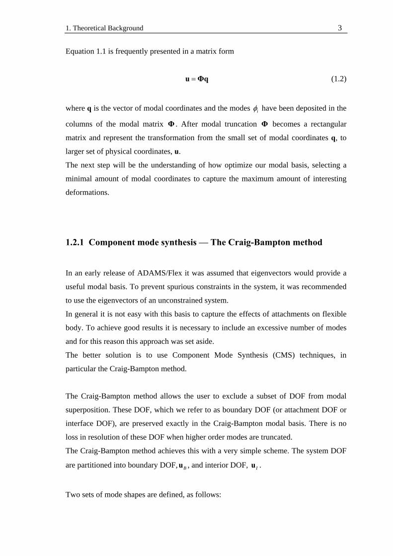
Equation 1.1 is frequently presented in a matrix form
=u Φq (1.2)
where q is the vector of modal coordinates and the modes iφ have been deposited in the
columns of the modal matrix Φ . After modal truncation Φ becomes a rectangular
matrix and represent the transformation from the small set of modal coordinates q, to
larger set of physical coordinates, u.
The next step will be the understanding of how optimize our modal basis, selecting a
minimal amount of modal coordinates to capture the maximum amount of interesting
deformations.
1.2.1 Component mode synthesis — The Craig-Bampton method
In an early release of ADAMS/Flex it was assumed that eigenvectors would provide a
useful modal basis. To prevent spurious constraints in the system, it was recommended
to use the eigenvectors of an unconstrained system.
In general it is not easy with this basis to capture the effects of attachments on flexible
body. To achieve good results it is necessary to include an excessive number of modes
and for this reason this approach was set aside.
The better solution is to use Component Mode Synthesis (CMS) techniques, in
particular the Craig-Bampton method.
The Craig-Bampton method allows the user to exclude a subset of DOF from modal
superposition. These DOF, which we refer to as boundary DOF (or attachment DOF or
interface DOF), are preserved exactly in the Craig-Bampton modal basis. There is no
loss in resolution of these DOF when higher order modes are truncated.
The Craig-Bampton method achieves this with a very simple scheme. The system DOF
are partitioned into boundary DOF, Bu , and interior DOF, Iu .
Two sets of mode shapes are defined, as follows:
1. Theoretical Background 4
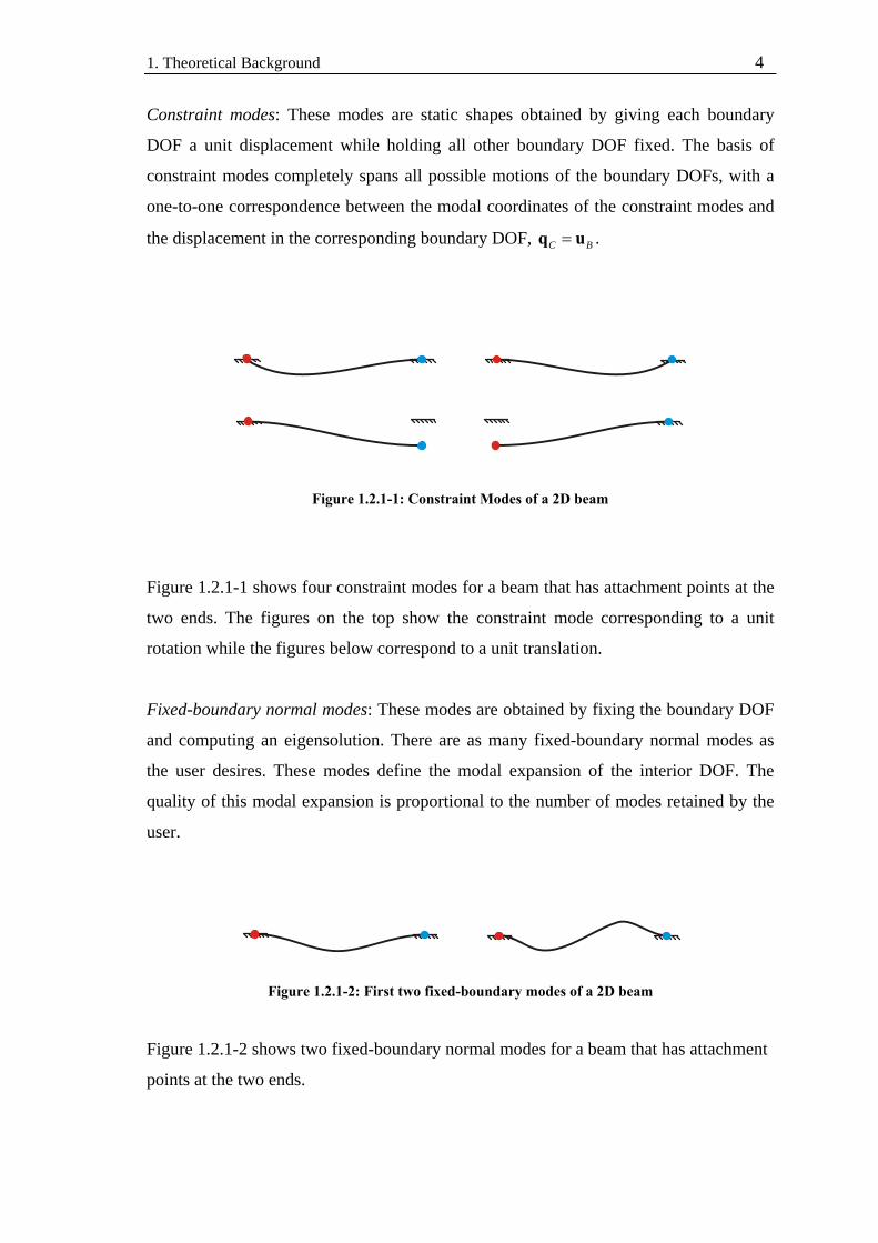
Constraint modes: These modes are static shapes obtained by giving each boundary
DOF a unit displacement while holding all other boundary DOF fixed. The basis of
constraint modes completely spans all possible motions of the boundary DOFs, with a
one-to-one correspondence between the modal coordinates of the constraint modes and
the displacement in the corresponding boundary DOF, C B=q u .
Figure 1.2.1-1: Constraint Modes of a 2D beam
Figure 1.2.1-1 shows four constraint modes for a beam that has attachment points at the
two ends. The figures on the top show the constraint mode corresponding to a unit
rotation while the figures below correspond to a unit translation.
Fixed-boundary normal modes: These modes are obtained by fixing the boundary DOF
and computing an eigensolution. There are as many fixed-boundary normal modes as
the user desires. These modes define the modal expansion of the interior DOF. The
quality of this modal expansion is proportional to the number of modes retained by the
user.
Figure 1.2.1-2: First two fixed-boundary modes of a 2D beam
Figure 1.2.1-2 shows two fixed-boundary normal modes for a beam that has attachment
points at the two ends.
1. Theoretical Background 5
The relationship between the physical DOF and the Craig-Bampton modes and their
modal coordinates is expressed by the following equation.
CB
IC IN NI
⎡ ⎤ ⎧ ⎫⎧ ⎫= =⎨ ⎬ ⎨ ⎬⎢ ⎥⎩ ⎭ ⎣ ⎦ ⎩ ⎭
I 0 quu
Φ Φ qu (1.3)
Where
Bu are the boundary DOF
Iu are the interior DOF
I, 0 are identity and zero matrices, respectively
ICΦ are the physical displacements of the interior DOF in the constraint modes
ICΦ are the physical displacements of the interior DOF in the normal modes
Cq the modal coordinates of the constraint modes
Nq the modal coordinates of the fixed-boundary normal modes
The generalized stiffness and mass matrices corresponding to the Craig-Bampton modal
basis are obtained via a modal transformation. The stiffness transformation is
ˆˆ
ˆ
TCCBB BIT
IC IN IC INIB II NN
⎡ ⎤⎡ ⎤ ⎡ ⎤⎡ ⎤= = = ⎢ ⎥⎢ ⎥ ⎢ ⎥⎢ ⎥
⎣ ⎦⎣ ⎦ ⎣ ⎦ ⎢ ⎥⎣ ⎦
I 0 I 0 K 0K KK Φ KΦ
Φ Φ Φ ΦK K 0 K (1.4)
while the mass transformation is
ˆ ˆˆ
ˆ ˆ
TCC NCBB BIT
IC IN IC INIB II CN NN
⎡ ⎤⎡ ⎤ ⎡ ⎤⎡ ⎤= = = ⎢ ⎥⎢ ⎥ ⎢ ⎥⎢ ⎥
⎣ ⎦⎣ ⎦ ⎣ ⎦ ⎢ ⎥⎣ ⎦
I 0 I 0 M MM MM Φ MΦ
Φ Φ Φ ΦM M M M (1.5)

1. Theoretical Background 6
where the subscripts I, B, N and C denote internal DOF, boundary DOF, normal mode
and constraint mode, respectively. The caret on M̂ and K̂ denotes that this is the
generalized mass and stiffness matrix.
Equations 1.4 and 1.5 have a few noteworthy properties:
• ˆNNM and ˆ
NNK are diagonal matrices because they are associated with
eigenvectors.
• K̂ is block diagonal. There is no stiffness coupling between the constraint
modes and fixed-boundary normal modes.
• M̂ is not block diagonal because there is inertia coupling between the constraint
modes and the fixed-boundary normal modes.
1.2.2 Mode shape orthonormalization
The Craig-Bampton method is a powerful method for tailoring the modal basis to
capture both the desired attachment effects and the desired level of dynamic content.
However, the raw Craig-Bampton modal basis has certain deficiencies that make it
unsuitable for direct use in a dynamic system simulation. These are:
1. Embedded in the Craig-Bampton constraint modes are 6 rigid body DOF which
must be eliminated before the ADAMS analysis because ADAMS provides its
own large-motion rigid body DOF.
2. The Craig-Bampton constraint modes are the result of a static condensation.
Consequently, these modes do not advertise the dynamic frequency content that
they contribute to the flexible system.
3. Craig-Bampton constraint modes cannot be disabled because to do so would be
equivalent to applying a constraint on the system.
These problems with the raw Craig-Bampton modal basis are resolved by applying a
simple mathematical operation on the Craig-Bampton modes.
1. Theoretical Background 7
The Craig-Bampton modes are not an orthogonal set of modes, as evidenced by the fact
that their generalized mass and stiffness matrices K̂ and M̂ , encountered in equations
1.4 and 1.5, are not diagonal.
By solving an eigenvalue problem
ˆ ˆλ=Kq Mq (1.6)
we obtain eigenvectors that we arrange in a transformation matrix N, which transforms
the Craig-Bampton modal basis to an equivalent, orthogonal basis with modal
coordinates
∗ =Nq q (1.7)
The effect on the superposition formula is
1 1 1
M M M
i i i ii i i
qφ φ φ∗ ∗ ∗
= = =
= = =∑ ∑ ∑u Nq q (1.8)
Where iφ∗ are the orthogonalized Craig-Bampton modes.
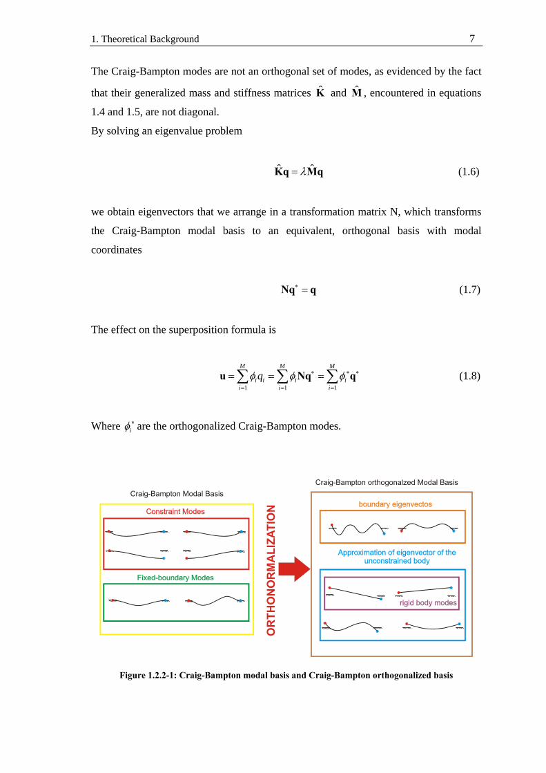
Figure 1.2.2-1: Craig-Bampton modal basis and Craig-Bampton orthogonalized basis
1. Theoretical Background 8
The orthogonalized Craig-Bampton modes are not eigenvectors of the original system.
They are eigenvectors of the Craig-Bampton representation of the system and as such
have a natural frequency associated with them. Figure 1.2.2-1 shows the effect of the
orthonormalization for the beam example. A physical description of these modes is
difficult, but in general the following is observed:
• Fixed-boundary normal modes are replaced with an approximation of the eigenvectors
of the unconstrained body. This is an approximation because it is based only on the
Craig-Bampton modes. Out of these modes, 6 modes are the rigid body modes.
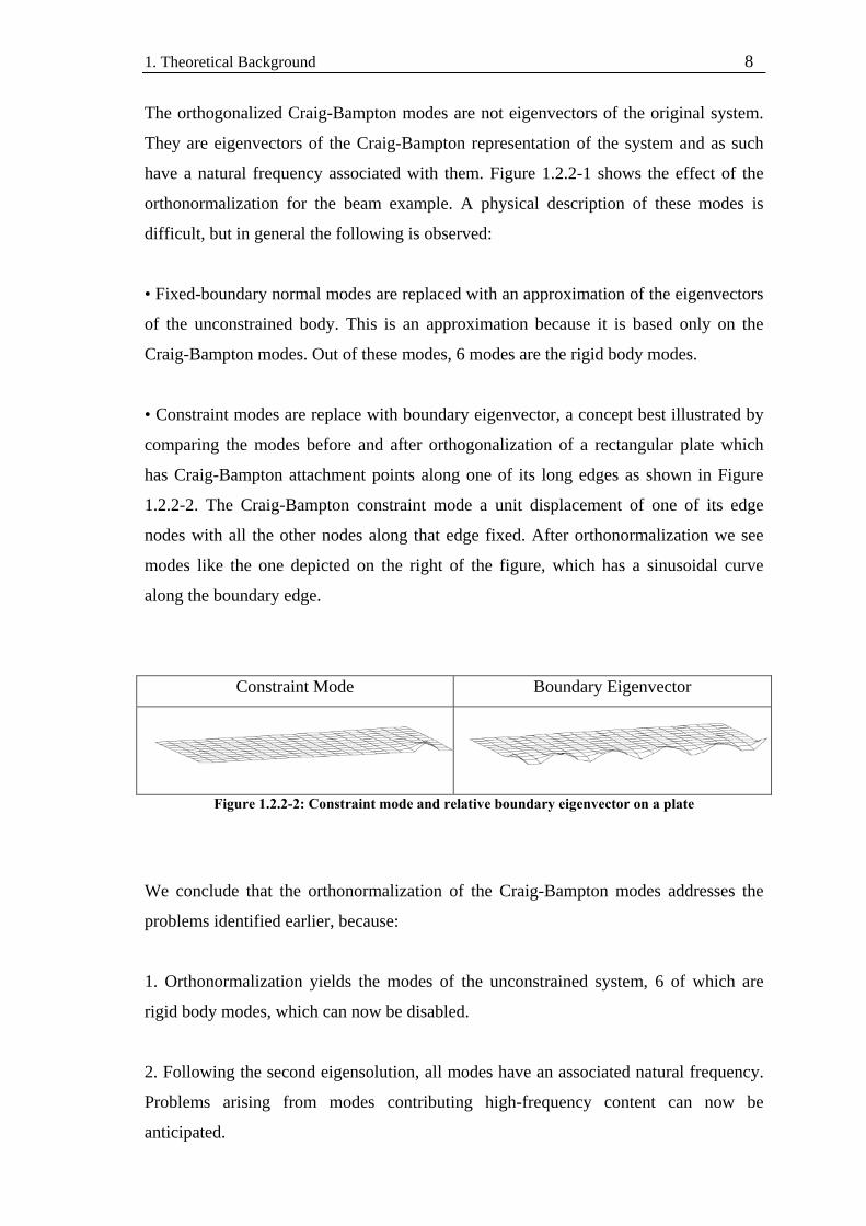
• Constraint modes are replace with boundary eigenvector, a concept best illustrated by
comparing the modes before and after orthogonalization of a rectangular plate which
has Craig-Bampton attachment points along one of its long edges as shown in Figure
1.2.2-2. The Craig-Bampton constraint mode a unit displacement of one of its edge
nodes with all the other nodes along that edge fixed. After orthonormalization we see
modes like the one depicted on the right of the figure, which has a sinusoidal curve
along the boundary edge.
Constraint Mode Boundary Eigenvector
Figure 1.2.2-2: Constraint mode and relative boundary eigenvector on a plate
We conclude that the orthonormalization of the Craig-Bampton modes addresses the
problems identified earlier, because:
1. Orthonormalization yields the modes of the unconstrained system, 6 of which are
rigid body modes, which can now be disabled.
2. Following the second eigensolution, all modes have an associated natural frequency.
Problems arising from modes contributing high-frequency content can now be
anticipated.

1. Theoretical Background 9
3. Although the removal of any mode constrains the body from adopting that particular
shape, the removal of a high-frequency such as the boundary eigenvector of Figure
1.2.2-2 is clearly more benign than removing the relative constraint mode. The removal
of the latter mode prevents the associated boundary node from moving relative to its
neighbors. Meanwhile, the removal of the former mode only prevents boundary edge
from reaching this degree of “waviness”.
1. Theoretical Background 10
1.3 Modal flexibility in ADAMS
In this section we show how ADAMS capitalizes on modal superposition in the two key
areas of the ADAMS formulation:
• Flexible marker kinematics
• Flexible body equations of motion
1.3.1 Flexible marker kinematics
Marker kinematics refers to the position, orientation, velocity, and acceleration of
markers. ADAMS uses the kinematics of markers in three key areas:
• Marker position and orientation must be known in order to satisfy constraints
like those imposed in JOINT and JPRIM elements.
• To project point forces applied at markers on generalized coordinates of the
flexible body.
• The marker measures, (for example DX, WZ, PHI, ACCX, and so on) that
appear in expressions and user-written subroutines require information about
position, orientation, velocity, and acceleration of markers
1.3.1.1 Position
Figure 1.3.1-1: Flexible body reference system in ADAMS
1. Theoretical Background 11
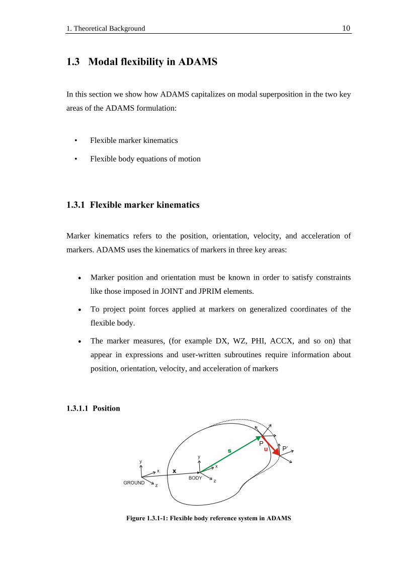
The instantaneous location of a marker that is attached to a node, P, on a flexible body,
B, is the sum of three vectors (see ).
p p pr x s u= + + (1.9)
Where
x is the position vector from the origin of the ground reference frame to the origin of
the local body reference frame, B, of the flexible body.
ps is the position vector of the undeformed position of point P with respect to the local
body reference frame of body B.
pu is the translational deformation vector of point P, the position vector from the point’s
undeformed position to its deformed position.
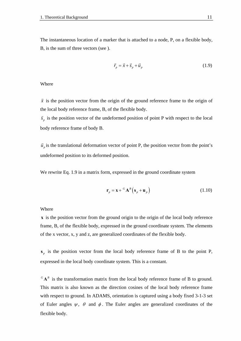
We rewrite Eq. 1.9 in a matrix form, expressed in the ground coordinate system
( )G Bp p p= + +r x A s u (1.10)
Where
x is the position vector from the ground origin to the origin of the local body reference
frame, B, of the flexible body, expressed in the ground coordinate system. The elements
of the x vector, x, y and z, are generalized coordinates of the flexible body.
ps is the position vector from the local body reference frame of B to the point P,
expressed in the local body coordinate system. This is a constant.
G BA is the transformation matrix from the local body reference frame of B to ground.
This matrix is also known as the direction cosines of the local body reference frame
with respect to ground. In ADAMS, orientation is captured using a body fixed 3-1-3 set
of Euler angles ,ψ θ and φ . The Euler angles are generalized coordinates of the
flexible body.
1. Theoretical Background 12
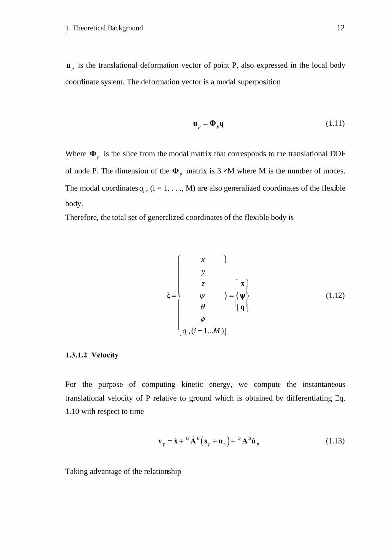
pu is the translational deformation vector of point P, also expressed in the local body
coordinate system. The deformation vector is a modal superposition
p p=u Φ q (1.11)
Where pΦ is the slice from the modal matrix that corresponds to the translational DOF
of node P. The dimension of the pΦ matrix is 3 ×M where M is the number of modes.
The modal coordinates iq , (i = 1, . . ., M) are also generalized coordinates of the flexible
body.
Therefore, the total set of generalized coordinates of the flexible body is
, ( 1... )i
xyz
q i M
ψθφ
⎧ ⎫⎪ ⎪⎪ ⎪⎪ ⎪ ⎧ ⎫⎪ ⎪ ⎪ ⎪= =⎨ ⎬ ⎨ ⎬⎪ ⎪ ⎪ ⎪
⎩ ⎭⎪ ⎪⎪ ⎪⎪ ⎪=⎩ ⎭
xξ ψ
q (1.12)
1.3.1.2 Velocity
For the purpose of computing kinetic energy, we compute the instantaneous
translational velocity of P relative to ground which is obtained by differentiating Eq.
1.10 with respect to time
( )G B G Bp p p p= + + +v x A s u A u (1.13)
Taking advantage of the relationship
1. Theoretical Background 13
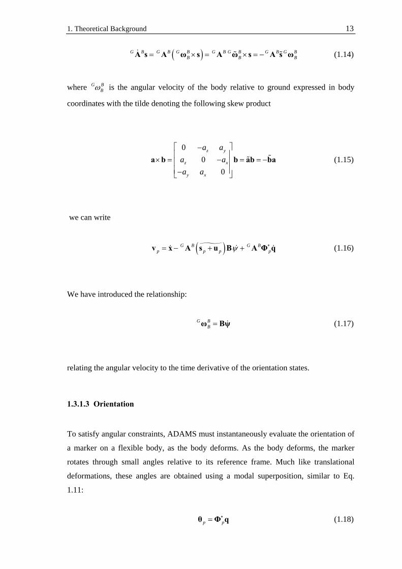
( )G B G B G B G B G B G B G BB B B= × = × = −A s A ω s A ω s A s ω (1.14)
where G BBω is the angular velocity of the body relative to ground expressed in body
coordinates with the tilde denoting the following skew product
0
00
z y
z x
y x
a aa aa a
⎡ ⎤−⎢ ⎥× = − = = −⎢ ⎥⎢ ⎥−⎣ ⎦
a b b ab ba (1.15)
we can write
( )G B G Bp p p pψ ∗= − + +v x A s u B A Φ q (1.16)
We have introduced the relationship:
G BB =ω Bψ (1.17)
relating the angular velocity to the time derivative of the orientation states.
1.3.1.3 Orientation
To satisfy angular constraints, ADAMS must instantaneously evaluate the orientation of
a marker on a flexible body, as the body deforms. As the body deforms, the marker
rotates through small angles relative to its reference frame. Much like translational
deformations, these angles are obtained using a modal superposition, similar to Eq.
1.11:
p p∗=θ Φ q (1.18)

1. Theoretical Background 14
Where p∗Φ is the slice from the modal matrix that corresponds to the rotational DOF of
node P. The dimension of the p∗Φ matrix is 3 ×M where M is the number of modes.
The orientation of marker J relative to ground is represented by the Euler transformation
matrix, G JA . This matrix is the product of three transformation matrices:
G J G B B P P J=A A A A (1.19)
Where
G BA is the transformation matrix from the local body reference frame of B to ground.
B PA is the transformation matrix due to the orientation change due to the deformation
of node P.
P JA is the constant transformation matrix that was defined by the user when the marker
was placed on the flexible body.
The matrix B PA requires more attention. The direction cosines for a vector of small
angles, pθ , are
1
11
pz pyB P
pz px p
py px
θ θθ θθ θ
⎡ ⎤−⎢ ⎥= − = +⎢ ⎥⎢ ⎥−⎣ ⎦
A I θ (1.20)
where the tilde denotes the skew operator (Eq. 1.15).
1. Theoretical Background 15
1.3.1.4 Angular velocity
The angular velocity of a marker, J, on a flexible body is the sum of the angular velocity
of the body and the angular velocity due to deformation
G J G P G B B P G BB B B B B p
∗= = + = +ω ω ω ω ω Φ q (1.21)
1.3.2 Applied loads
The treatment of forces in ADAMS distinguishes between point loads and distributed
loads. This section will focus only on he point forces and torque since they are the only
of interest for the models that will be developed in further chapters.
1.3.2.1 Point forces and torques
A point force F and a point torque T that are applied to a marker on a flexible body
must be projected on the generalized coordinates of the system.
The force and torque are written in matrix form, and expressed in the coordinate system
of marker K.
x x
K y K y
z z
f tf tf t
⎡ ⎤ ⎡ ⎤⎢ ⎥ ⎢ ⎥= =⎢ ⎥ ⎢ ⎥⎢ ⎥ ⎢ ⎥⎣ ⎦ ⎣ ⎦
F T (1.22)
The generalized force Q consists of a generalized translational force, a generalized
torque (a generalized force on the Euler angles) and a generalized modal force, thus:
T
R
M
⎡ ⎤⎢ ⎥= ⎢ ⎥⎢ ⎥⎣ ⎦
QQ Q
Q (1.23)
1. Theoretical Background 16
Generalized Translational Force: Since the governing equations of motion, Eq. 1.42,
are written in the global reference frame, the generalized force on the translational
coordinates is obtained by transforming KF to global coordinates.
G KT K=Q A F (1.24)
where G KA is given in Eq. 1.19. The generalized translational force is independent of
the point of force application.
An applied torque does not contribute to TQ .
Generalized Torque: The total torque on a flexible body, due to F and T is
TOTT T p F= + × , where p is the position vector from the origin of the local body
reference frame of the body to the point of force application. The total torque, can be
written in matrix form, with respect to the ground coordinate system as:
G K G KTOT K K= + ×T A T p A F (1.25)
Where p is expressed in the ground coordinates. Using the tilde notation of Eq. 1.20
this can be written as
G K G KTOT K K= +T A T p A F (1.26)
The transformation from torque in physical coordinates to the generalized torque on the
body Euler angles is provided by the B matrix in Eq. 1.16
T TG K G K G K G K
R TOT K K⎡ ⎤ ⎡ ⎤ ⎡ ⎤= = +⎣ ⎦ ⎣ ⎦ ⎣ ⎦Q A B T A B A T p A F (1.27)
1. Theoretical Background 17
Generalized Modal Force: The generalized modal force on a body due to applied point
forces or point torques at P is obtained by projecting the load on the mode shapes.
As the applied force KF and torque KT are given with respect to marker K, they must
first be transformed to the reference frame of the flexible body
TG B G K
I K⎡ ⎤= ⎣ ⎦F A A F (1.28)
TG B G K
I K⎡ ⎤= ⎣ ⎦T A A T (1.29)
and then projected on the mode shapes. The force is projected on the translational mode
shapes and the torque is projected on the angular mode shapes
T TF p I p I
∗= +Q Φ F Φ T (1.30)
Where pΦ and p∗Φ slices of the modal matrix corresponding to the translational and
angular DOF of point P, as discussed in section 1.3.1.
Note that since the modal matrix Φ is only defined at nodes, point forces and point
torques can only be applied at nodes.
1.3.3 Flexible body equations of motion
The governing equations for a general multi body system are derived from Lagrange’s
equations of the form
0
0
Td L Ldt
⎧ ⎛ ⎞ ⎡ ⎤∂ ∂ ∂ ∂− + + − =⎪ ⎜ ⎟ ⎢ ⎥∂ ∂∂ ∂⎨ ⎣ ⎦⎝ ⎠
⎪ =⎩
Ψ λ Qξ ξξ ξ
Ψ
F (1.31)

1. Theoretical Background 18
Where
L is the Lagrangian, defined below
F is an energy dissipation function, defined below
Ψ are the constraint equations
λ are the Lagrange multipliers for the constraints
ξ are the generalized coordinates as defined in Eq. 1.12
Q are the generalized applied forces (the applied forces projected on �)
The Lagrangian is defined as
L T V= −
where T and V denote kinetic and potential energy respectively.
The remainder of this section is devoted to the derivation of the contributions to Eq.
1.41, in the following order:
• Kinetic energy and the mass matrix
• Potential energy and the stiffness matrix
• Dissipation and the damping matrix
• Constraints
1.3.3.1 Kinetic energy and the mass matrix
The velocity from Eq. 1.16 can be expressed in terms of the time derivative of the state
vector
[ ] ( ) G B G Bp p p p
⎡ ⎤⎡ ⎤ ⎡ ⎤= − + ⋅⎣ ⎦⎣ ⎦⎣ ⎦v I A s u B A Φ ξ (1.32)
We can now compute the kinetic energy. The kinetic energy for a flexible body is given
as
1. Theoretical Background 19
1 12 2
T T G BT G Bp p p P p P
pV
T dV mρ= ≈ +∑∫ v v v v ω I ω (1.33)
where mp and pI are the nodal mass and nodal inertia tensor of node P, respectively.
Note that pI is often a negligible quantity which arises when reduced continuum
descriptions, i.e. bars, beams, or shells, are employed in your flexible component model.
Lumped masses and inertia may also contribute to this term.
Substituting for v and ω and simplifying yields an equation for the kinetic energy in
ADAMS’ generalized mass matrix and generalized coordinates.
( )12
TT = ξ M ξ ξ (1.34)
For clarity of presentation we partition the mass matrix, ( )M ξ , into a 3 × 3 block
matrix
( )tt tr tmTtr rr rmT Ttm rm mm
⎡ ⎤⎢ ⎥= ⎢ ⎥⎢ ⎥⎣ ⎦
M M MM ξ M M M
M M M (1.35)
where the subscripts t, r and m denote translational, rotational, and modal DOF
respectively.
The expression for the mass matrix ( )M ξ simplifies to an expression in nine inertia
invariants.
1
2 3
3
7 8 8 9
4 5
6
tt
tr j j
tm
T Trr j j j ij i j
Trm j j
mm
q
q q q
q
⎧ =⎪
⎡ ⎤= − +⎪ ⎣ ⎦⎪
=⎪⎨ ⎡ ⎤⎡ ⎤= − + −⎪ ⎣ ⎦⎣ ⎦⎪
⎡ ⎤= −⎪ ⎣ ⎦⎪
=⎩
M I
M A B
M A
M B B
M B
M
I
I I
I
I I I I
I I
I
(1.36)

1. Theoretical Background 20
The explicit dependence of the mass matrix on the modal coordinates is evident. The
dependence on orientation coordinates of the system comes about because of the
transformation matrices A and B.
The inertia invariants are computed from the N nodes of the finite element model based
on information about each node’s mass, pm , its undeformed location ps , and its
participation in the component modes pΦ . The discrete form of the inertia invariants
are provided in Table 1.1.
1
1
N
pp
m=
= ∑I Scalar
2
1
N
p pp
m=
=∑ sI (3 1)×
3
1
N
j p pp
m=
= ∑ ΦI 1,...,j M= (3 )M×
4
1
N
p p p p pp
m=
′= +∑ s Φ I ΦI (3 )M×
5
1
N
j p pj pp
m φ=
=∑ ΦI 1,...,j M= (3 )M×
6
1
NT T
p p p p p pp
m=
′ ′= +∑ Φ Φ Φ I ΦI ( )M M×
7
1
NT
p p p pp
m=
= +∑ s s II (3 3)×
8
1
N
j p p pjp
m φ=
=∑ sI 1,...,j M= (3 3)×
9
1
N
jk p pj pkp
m φ φ=
=∑I , 1,...,j k M= (3 3)×
Table 1-1: Discrete form of inertia invariants
1. Theoretical Background 21
1.3.3.2 Potential energy and the stiffness matrix
Frequently, the potential energy consists of contributions from gravity and elasticity in
the quadratic form.
( ) 12
TgV V= +ξ ξ Kξ (1.37)
In the elastic energy term, K is the generalized stiffness matrix which is, in general,
constant. Only the modal coordinates, q, contribute to the elastic energy. Therefore, the
form of K is
0 0 00 0 00 0
tt tr tmTtr rr rmT Ttm rm mm mm
⎡ ⎤ ⎡ ⎤⎢ ⎥ ⎢ ⎥= =⎢ ⎥ ⎢ ⎥⎢ ⎥ ⎢ ⎥⎣ ⎦ ⎣ ⎦
K K KK K K K
K K K K (1.38)
where mmK is the generalized stiffness matrix of the structural component with respect
to the modal coordinates, q. It is not the full structural stiffness matrix of the
component.
gV is the gravitational potential energy,
( ) ( )T
g p pV V
V dV P dVρ ρ ⎡ ⎤= ⋅ = + +⎣ ⎦∫ ∫r g x A s Φ q g (1.39)
where g denotes the gravitational acceleration vector. The resulting gravitational force is
( ) ( )
( )
V
TTgg p
V
T T
V
dV
VP dV
P dV
ρ
ρ
ρ
⎡ ⎤⎡ ⎤⎢ ⎥⎢ ⎥
⎣ ⎦⎢ ⎥⎢ ⎥∂ ⎡ ⎤ ∂⎢ ⎥= = +⎢ ⎥⎢ ⎥∂ ∂⎣ ⎦⎢ ⎥⎢ ⎥⎡ ⎤⎢ ⎥⎢ ⎥⎢ ⎥⎣ ⎦⎣ ⎦
∫
∫
∫
g
Af s Φ q gξ ψ
Φ A g
(1.40)

1. Theoretical Background 22
1.3.3.3 Dissipation and the damping matrix
The damping forces depend on the generalized modal velocities and are assumed to be
derivable from the quadratic form
12
T= q DqF (1.41)
which is known as Rayleigh’s dissipation function. The matrix D contains the damping
coefficients, ijd , and is generally constant and symmetric. In the case of orthogonal
mode shapes, the damping matrix can be effectively defined using a diagonal matrix of
modal damping ratios, ic . This damping ratio could be different for each of the
orthogonal modes and can be conveniently defined as a ratio of the critical damping for
the mode, cric (where the critical damping ratio is defined as the level of damping that
eliminates harmonic response).
1.3.3.4 Constraints
ADAMS satisfies position and orientation constraints for flexible body markers by
using the marker kinematics properties presented in section 1.3.1.
1.3.3.5 Governing differential equation of motion — final form
The final form of the governing differential equation of motion, in terms of the
generalized coordinates is
1 02
T T
g⎡ ⎤ ⎡ ⎤∂ ∂
+ − + + + + − =⎢ ⎥ ⎢ ⎥∂ ∂⎣ ⎦ ⎣ ⎦
M ΨMξ Mξ ξ ξ Kξ f Dξ λ Qξ ξ
(1.42)

1. Theoretical Background 23
The entries in Eq. 1.42 are:
ξ ,ξ ,ξ the flexible body generalized coordinates and their time derivatives
M the flexible body mass matrix in Eq. 1.34
M the time derivative of the flexible body mass matrix
∂∂Mξ
the partial derivative of the mass matrix with respect to the flexible body
generalized coordinates. This is a (M + 6) × (M + 6) × (M + 6) tensor, where M
is the number of modes
K the generalized stiffness matrix
gf the generalized gravitational force
D the modal damping matrix
Ψ the algebraic constraint equations
λ Lagrange multipliers for the constraints
Q generalized applied force
Chapter 2 The Rigid Model
2.1 The rigid model objective
The objective of a rigid analysis is to simulate and asses the operational quality of the
deployment function of a solar array.
The rigid model focus mainly on two aspects
• Torque Margin Analysis
A quasi static analysis that has to demonstrate the motorization margin of safety for
a deployment worst case approach (cold case). The worst case approach comprises
the highest resistive forces and torques occurring at a cold temperature extreme
condition (higher frictions). The solar array has to keep deploying and reach the
deployed configuration even if it is stopped in a partial-deployed configuration.

2. The Rigid Model 25
• Dynamic Load Analysis
A dynamic analysis that has to determinate the maximum reaction loads onto the
structure of the solar array. This aspect reflects in general lowest resistive magnitude
and highest motorization magnitudes of related components.
Usually the first analysis fixes the motorization items of the deployment mechanism. If,
for example, the deployment is obtained using deployment springs this analysis will
settle their stiffness and their wind-up angles.
The requirements on the torque margin, according to ESA ECSS rule, impose a margin
of 2:1 between the driving torque versus resistive torque with uncertainty factors
included.
The success criteria for torque margin are defined, at each Hinge Line (HL) through the
following formula.
2 for 1, 2,3jj
j
DTM j
RΣ
= ≥ =Σ
(2.1)
jDΣ = sum of driving torque at HL #j
jRΣ = sum of resistive torque at HL #j with UFs included
Due to the strict requirements the potential energy that at the end will be stored in the
mechanism will be quite high and for this reason we need to calculate the dynamic
loads. In fact all this surplus of energy could generate high shock loads at the latch-ups.
It’s clear that with the flexible model investigation we will be interested in a better
comprehension of all the dynamic effects of this second analysis.
2.2 The ADAMS rigid model
A solar array wing is modelled as a mechanical Multiple Body System (MBS). The
equation of motion consist of a system of non-linear coupled differential and algebraic
equations due to large displacements and rotations during the deployment process. The
related mathematical model is set up with the MBS software package ADAMS.
2. The Rigid Model 26
Using this software we can create a 3D model of our solar array and analyse the
kinematical and dynamic behaviour for in-orbit or on-ground deployment.
The rigid model usually takes into account the following physical effects:
• Inertia of bodies
• Motorization spring torque
• Friction : Bearing friction in the hinges
Friction between cam and latch-up pin
• Harness torque effects
• Optional Closed Cable Loop (CCL) synchronization mechanism
• Optional dampers or engine holding torque
• Latch up of deployment hinges
• Bending Stiffness of solar array structure collocated in the HLs
• Aerodynamic loads (on-ground test simulation)
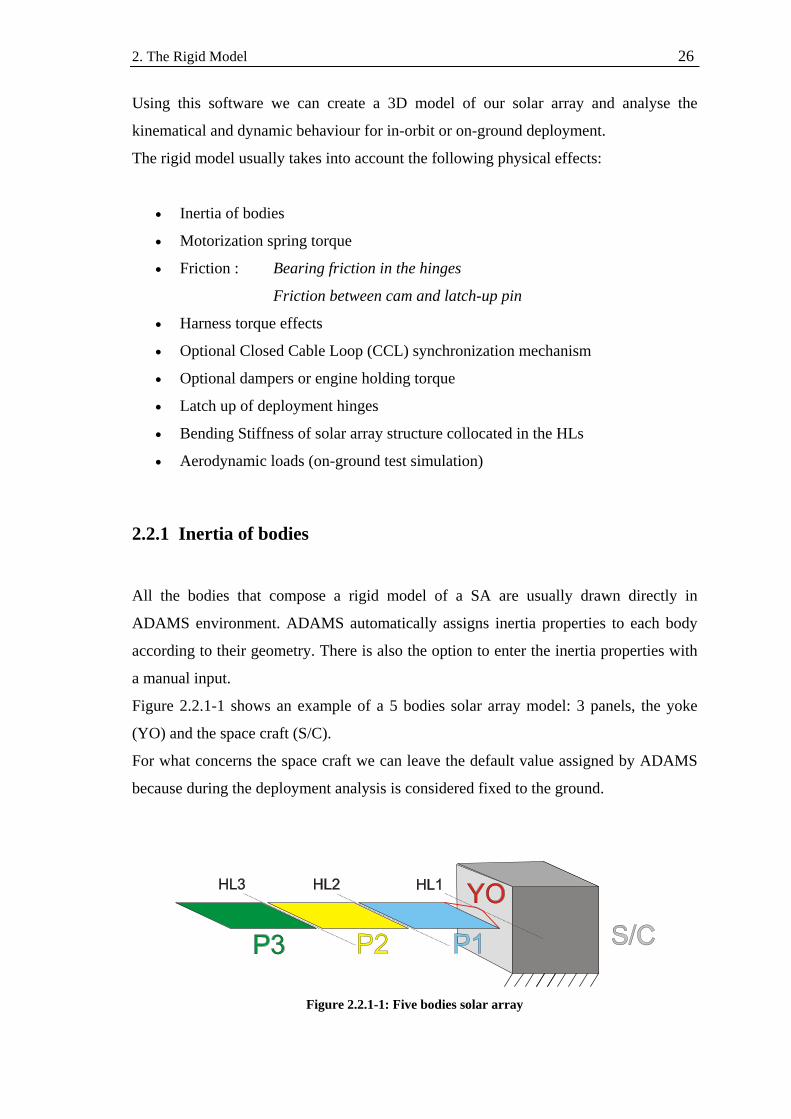
2.2.1 Inertia of bodies
All the bodies that compose a rigid model of a SA are usually drawn directly in
ADAMS environment. ADAMS automatically assigns inertia properties to each body
according to their geometry. There is also the option to enter the inertia properties with
a manual input.
Figure 2.2.1-1 shows an example of a 5 bodies solar array model: 3 panels, the yoke
(YO) and the space craft (S/C).
For what concerns the space craft we can leave the default value assigned by ADAMS
because during the deployment analysis is considered fixed to the ground.
Figure 2.2.1-1: Five bodies solar array
2. The Rigid Model 27
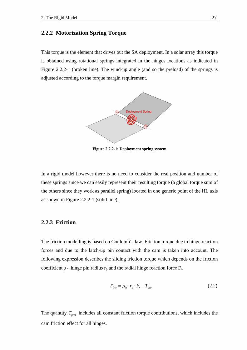
2.2.2 Motorization Spring Torque
This torque is the element that drives out the SA deployment. In a solar array this torque
is obtained using rotational springs integrated in the hinges locations as indicated in
Figure 2.2.2-1 (broken line). The wind-up angle (and so the preload) of the springs is
adjusted according to the torque margin requirement.
Figure 2.2.2-1: Deployment spring system
In a rigid model however there is no need to consider the real position and number of
these springs since we can easily represent their resulting torque (a global torque sum of
the others since they work as parallel spring) located in one generic point of the HL axis
as shown in Figure 2.2.2-1 (solid line).
2.2.3 Friction
The friction modelling is based on Coulomb’s law. Friction torque due to hinge reaction
forces and due to the latch-up pin contact with the cam is taken into account. The
following expression describes the sliding friction torque which depends on the friction
coefficient μh, hinge pin radius rp and the radial hinge reaction force Fr.
fric h p r pretT r F Tμ= ⋅ ⋅ + (2.2)
The quantity pretT includes all constant friction torque contributions, which includes the
cam friction effect for all hinges.
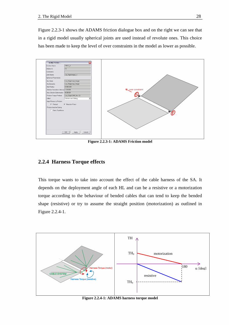
2. The Rigid Model 28
Figure 2.2.3-1 shows the ADAMS friction dialogue box and on the right we can see that
in a rigid model usually spherical joints are used instead of revolute ones. This choice
has been made to keep the level of over constraints in the model as lower as possible.
Figure 2.2.3-1: ADAMS Friction model
2.2.4 Harness Torque effects
This torque wants to take into account the effect of the cable harness of the SA. It
depends on the deployment angle of each HL and can be a resistive or a motorization
torque according to the behaviour of bended cables that can tend to keep the bended
shape (resistive) or try to assume the straight position (motorization) as outlined in
Figure 2.2.4-1.
Figure 2.2.4-1: ADAMS harness torque model
motorization
resistive
TH0
TH0
180
TH
α [deg]
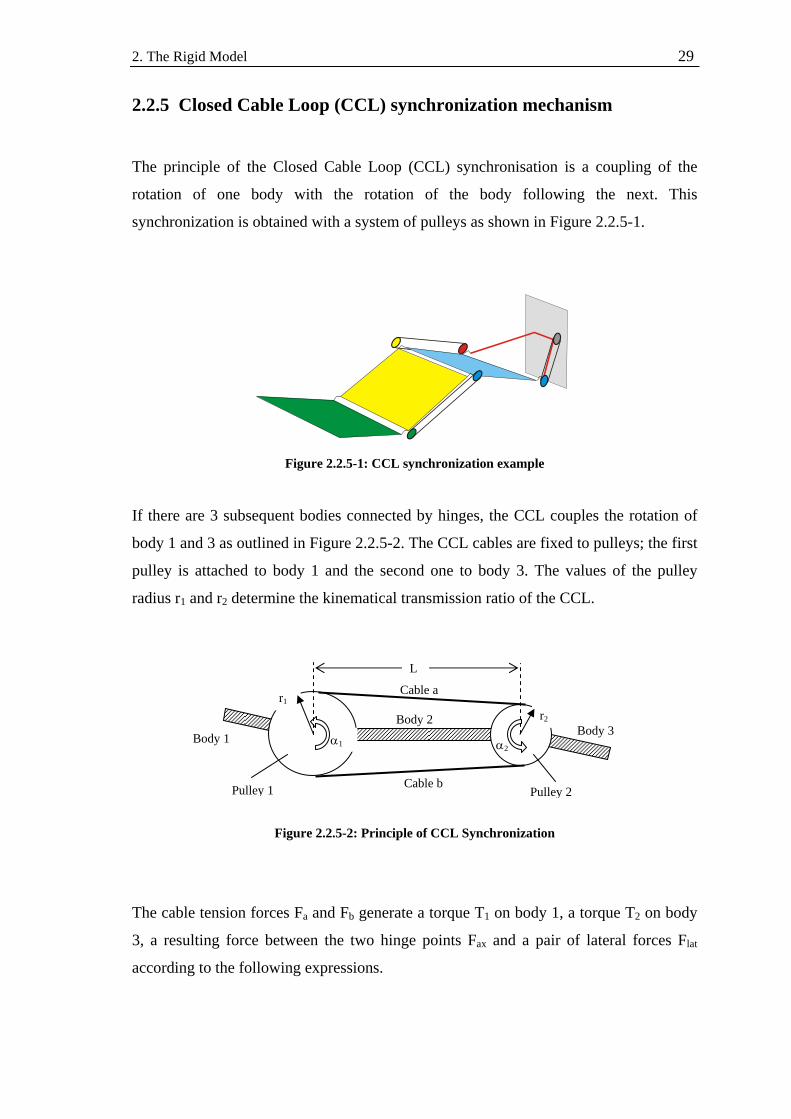
2. The Rigid Model 29
2.2.5 Closed Cable Loop (CCL) synchronization mechanism
The principle of the Closed Cable Loop (CCL) synchronisation is a coupling of the
rotation of one body with the rotation of the body following the next. This
synchronization is obtained with a system of pulleys as shown in Figure 2.2.5-1.
Figure 2.2.5-1: CCL synchronization example
If there are 3 subsequent bodies connected by hinges, the CCL couples the rotation of
body 1 and 3 as outlined in Figure 2.2.5-2. The CCL cables are fixed to pulleys; the first
pulley is attached to body 1 and the second one to body 3. The values of the pulley
radius r1 and r2 determine the kinematical transmission ratio of the CCL.
Figure 2.2.5-2: Principle of CCL Synchronization
The cable tension forces Fa and Fb generate a torque T1 on body 1, a torque T2 on body
3, a resulting force between the two hinge points Fax and a pair of lateral forces Flat
according to the following expressions.
Body 3
Cable a
Cable b
Body 1 Body 2
α1 α2
r1 r2
Pulley 1 Pulley 2
L

2. The Rigid Model 30
( )1 1 b aT r F F= ⋅ − (2.3) ( )2 2 a bT r F F= ⋅ − (2.4)
( )2 2
1 2
( )ax a bLF F F
r r L= + ⋅
− + (2.5)
( )
1 22 2
1 2
( )lat a br rF F F
r r L
−= − ⋅
− + (2.6)
The torques and forces on body 1 and body 3 generated by the CCL are outlined in
Figure 2.2.5-3. The lateral force only occurs if the two pulleys have a different radius.
Figure 2.2.5-3: Torques and Forces generated by CCL
The resulting torque on the yoke due to the guided CCL cables is outlined in Figure
2.2.5-4.
Figure 2.2.5-4: Torque on Yoke due to guided CCL cables
Body 3
Flat
Flat
Fax
Cable a
Cable b
Body 1
Pulley 1 Pulley 2
T1 T2
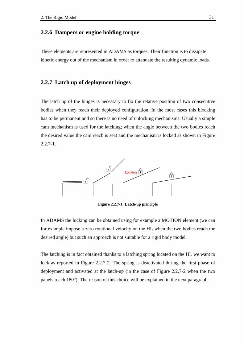
2. The Rigid Model 31
2.2.6 Dampers or engine holding torque
These elements are represented in ADAMS as torques. Their function is to dissipate
kinetic energy out of the mechanism in order to attenuate the resulting dynamic loads.
2.2.7 Latch up of deployment hinges
The latch up of the hinges is necessary to fix the relative position of two consecutive
bodies when they reach their deployed configuration. In the most cases this blocking
has to be permanent and so there is no need of unlocking mechanisms. Usually a simple
cam mechanism is used for the latching; when the angle between the two bodies reach
the desired value the cam reach is seat and the mechanism is locked as shown in Figure
2.2.7-1.
Figure 2.2.7-1: Latch-up principle
In ADAMS the locking can be obtained using for example a MOTION element (we can
for example impose a zero rotational velocity on the HL when the two bodies reach the
desired angle) but such an approach is not suitable for a rigid body model.
The latching is in fact obtained thanks to a latching spring located on the HL we want to
lock as reported in Figure 2.2.7-2. The spring is deactivated during the first phase of
deployment and activated at the latch-up (in the case of Figure 2.2.7-2 when the two
panels reach 180°). The reason of this choice will be explained in the next paragraph.

2. The Rigid Model 32
Figure 2.2.7-2: Example of latch-up obtained by a latching spring
2.2.8 Bending Stiffness of solar array structure collocated in the HLs
The problem that emerges with a full rigid model is that this model is not suitable for
dynamic analysis. For example the stresses on panels generated by the latching shock
would reach extremely high value (theoretically infinitive) because of the infinitive
stiffness of the structure involved in the latch-up. It’s clear that such an output would be
completely useless for our dynamic analysis.
This problem can be avoided introducing a concentrated stiffness on the hinge line as
shown in Figure 2.2.7-2. The structural stiffness of the two latched bodies will be
condensed in just one rotational DOF (one spring for each latched-up HL).
To tune these springs we will use a linear modes analysis and we will try to match the
frequency of the lower flexible mode of the FEM model with the adjusted stiffness of
the latch-up spring.
FEM
RIG
ID
Figure 2.2.8-1: Latch-up spring tuning
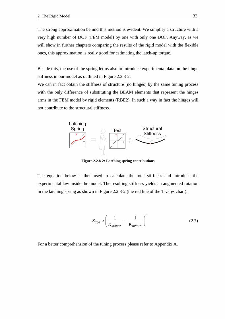
2. The Rigid Model 33
The strong approximation behind this method is evident. We simplify a structure with a
very high number of DOF (FEM model) by one with only one DOF. Anyway, as we
will show in further chapters comparing the results of the rigid model with the flexible
ones, this approximation is really good for estimating the latch-up torque.
Beside this, the use of the spring let us also to introduce experimental data on the hinge
stiffness in our model as outlined in Figure 2.2.8-2.
We can in fact obtain the stiffness of structure (no hinges) by the same tuning process
with the only difference of substituting the BEAM elements that represent the hinges
arms in the FEM model by rigid elements (RBE2). In such a way in fact the hinges will
not contribute to the structural stiffness.
Figure 2.2.8-2: Latching spring contributions
The equation below is then used to calculate the total stiffness and introduce the
experimental law inside the model. The resulting stiffness yields an augmented rotation
in the latching spring as shown in Figure 2.2.8-2 (the red line of the T vs ϕ chart).
1
1 1 TOTSTRUCT HINGES
KK K
−⎛ ⎞
≅ +⎜ ⎟⎝ ⎠
(2.7)
For a better comprehension of the tuning process please refer to Appendix A.

2. The Rigid Model 34
2.3 Applied Examples
In the following paragraph we will show two examples of rigid modelling.
• BEPI COLOMBO Mercury Polar Orbiter (MPO) solar array
• AMOS-3 solar array
- In orbit model
- On ground model
We have chosen these two examples because they cover the major part of applied
solutions. More complex solar arrays (with more panels) can be easily obtained from
this two models (see Chapter 5). The results of the rigid dynamic analysis will be
reported in Chapter 4 and directly compared with the relative results obtained from the
flexible analysis.

2. The Rigid Model 35
2.3.1 BEPI COLOMBO MPO solar array – Rigid model
The model consist of 3 rigid bodies, the space craft, the yoke with integrated inboard
panel and the out-board panel. The in-board and out-board panel are connected by
hinges like a double hinged door. The hinge (one revolute joint) between the SC and in-
board panel represent the Solar Array Drive Mechanism (SADM).
Figure 2.3.1-1: BEPI COLOMBO MPO solar array
The deployment motion is driven by deployment spring elements in HL2. There are two
further rotational springs in HL2, one represents the harness torque and the second one
represents the latch-up stiffness. The latter spring is deactivated during the deployment
process and is activated when the latch-up occurs.
After release of the hold-down mechanisms the out-board panel jumps out and starts
with the spring driven deployment. The latch-up occurs at a deployment angle of 180°.
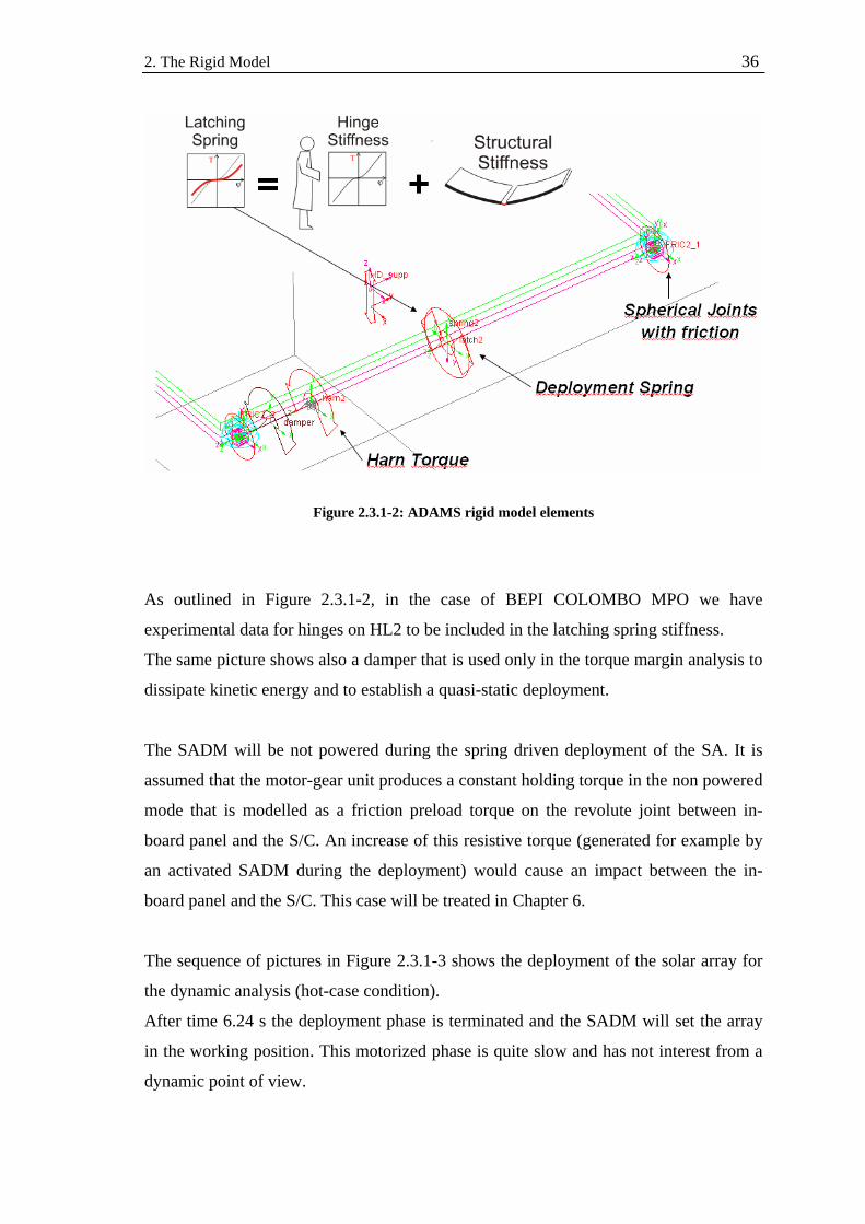
2. The Rigid Model 36
Figure 2.3.1-2: ADAMS rigid model elements
As outlined in Figure 2.3.1-2, in the case of BEPI COLOMBO MPO we have
experimental data for hinges on HL2 to be included in the latching spring stiffness.
The same picture shows also a damper that is used only in the torque margin analysis to
dissipate kinetic energy and to establish a quasi-static deployment.
The SADM will be not powered during the spring driven deployment of the SA. It is
assumed that the motor-gear unit produces a constant holding torque in the non powered
mode that is modelled as a friction preload torque on the revolute joint between in-
board panel and the S/C. An increase of this resistive torque (generated for example by
an activated SADM during the deployment) would cause an impact between the in-
board panel and the S/C. This case will be treated in Chapter 6.
The sequence of pictures in Figure 2.3.1-3 shows the deployment of the solar array for
the dynamic analysis (hot-case condition).
After time 6.24 s the deployment phase is terminated and the SADM will set the array
in the working position. This motorized phase is quite slow and has not interest from a
dynamic point of view.
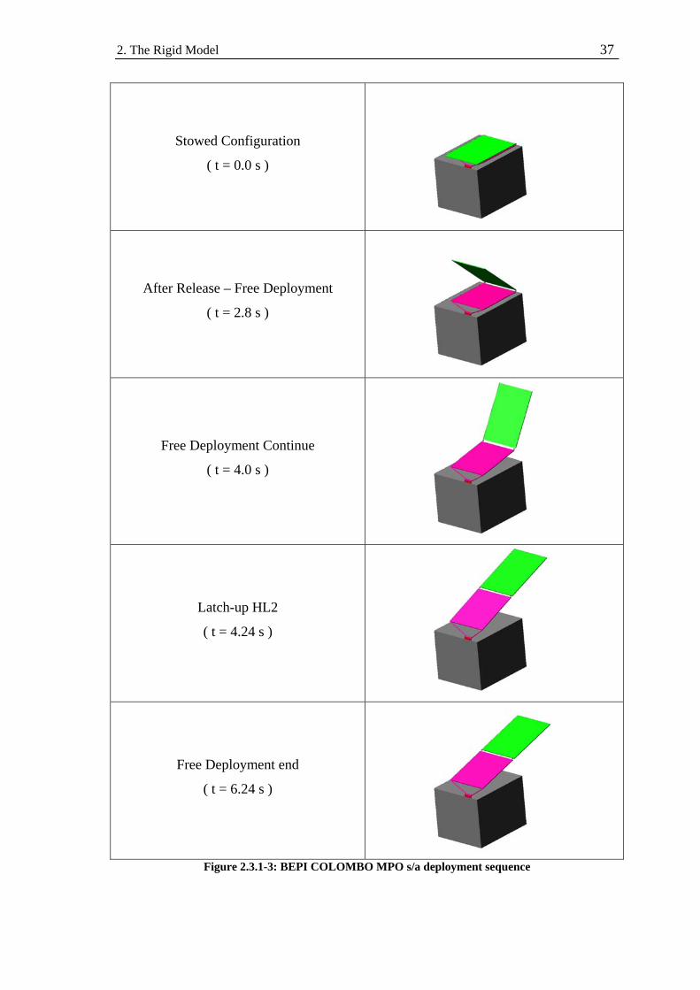
2. The Rigid Model 37
Stowed Configuration
( t = 0.0 s )
After Release – Free Deployment
( t = 2.8 s )
Free Deployment Continue
( t = 4.0 s )
Latch-up HL2
( t = 4.24 s )
Free Deployment end
( t = 6.24 s )
Figure 2.3.1-3: BEPI COLOMBO MPO s/a deployment sequence

2. The Rigid Model 38
2.3.2 AMOS-3 solar array – Rigid model
2.3.2.1 In orbit model
The total model consists of 4 rigid bodies, one for the SADM, one for the yoke and one
for each panel. The SADM body is fixed to the S/C, which represents the ground of the
simulation model. SADM, yoke and the two panels are connected by hinges like a
double hinged door.
Figure 2.3.2-1: AMOS-3 solar array (in-orbit)
The deployment motion is driven by deployment spring elements in HL1, 2 and 3. The
rotation in HL1 is damped by an Eddy Current damper element.
There are two further springs in each hinge-line, one represents the harness torque and
the second one represents the latch-up device with a representative locking stiffness.
The latter spring is deactivated during the deployment process and is activated when the
latch-up occurs in the related hinge-line.
Non-linear torque / force elements apply the synchronization torque at the bodies, and
account for the forces resulting from the CCL cables.
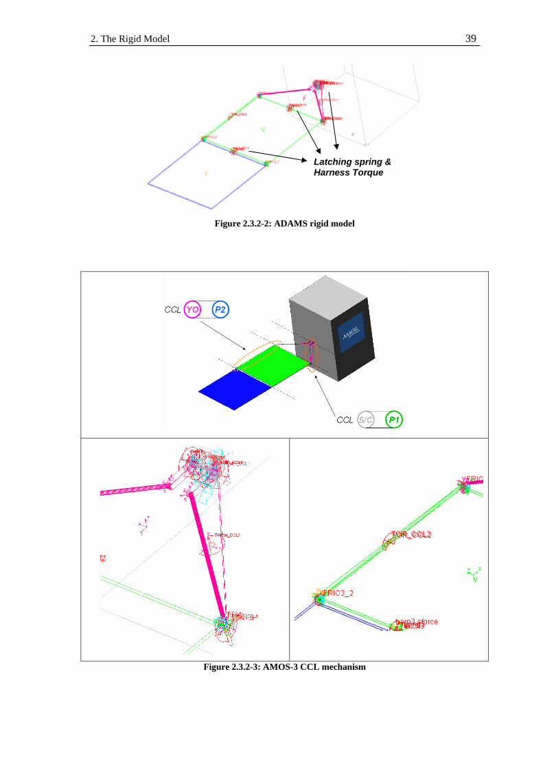
2. The Rigid Model 39
Figure 2.3.2-2: ADAMS rigid model
Figure 2.3.2-3: AMOS-3 CCL mechanism
Latching spring & Harness Torque

2. The Rigid Model 40
Figure 2.3.2-3 shows the CCL system in AMOS-3 solar array. The lines that appear in
the ADAMS rigid model are just geometrical lines used to graphically represent the two
CCL’s ; as we have seen in Figure 2.2.5-4 the CCL’s are represented in the model using
the resulting forces and torques. The inertial properties of pulleys are included in the
body to which they are linked to.
For what concern the latch-up stiffness in AMOS-3 case we have no experimental data.
That means that this time for the tuning of the latching spring we will use the FEM
mesh without substituting any rigid element. In other word the stiffness of the hinges
arms will coincide with the stiffness of the BEAM elements used to model them inside
the FEM model (see paragraph 2.2.8 ).
Figure 2.3.2-4 shows a sequence of the deployment. Notice the effect of the CCL
system in the rotation synchronization of the three bodies.

2. The Rigid Model 41
Stowed Configuration
( t = 0.0s )
After Release – Free
Deployment
( t = 4.0 s )
Free Deployment Continue
( t = 6.0 s )
Latch-up HL3
( t = 7.4 s )
Latch-up HL2
( t = 8.5 s )
Latch-up HL1
( t = 11.6s )
Fully Deployed Configuration
Figure 2.3.2-4: AMOS-3 deployment sequence
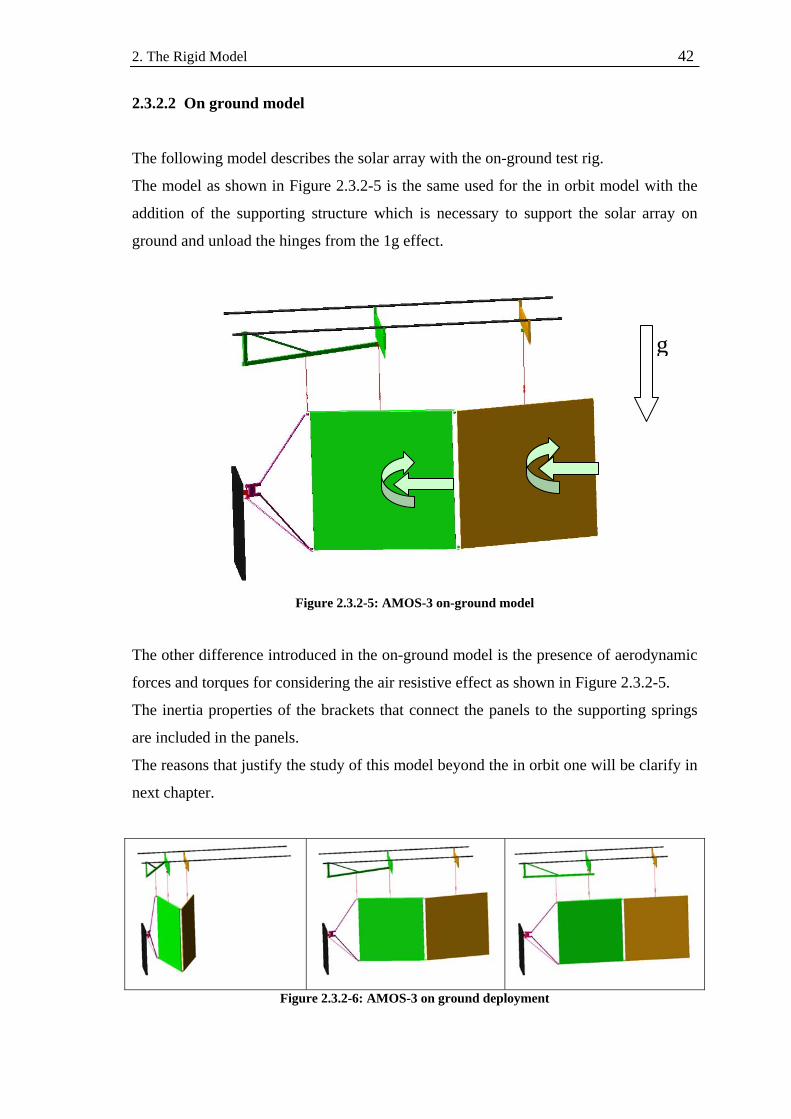
2. The Rigid Model 42
2.3.2.2 On ground model
The following model describes the solar array with the on-ground test rig.
The model as shown in Figure 2.3.2-5 is the same used for the in orbit model with the
addition of the supporting structure which is necessary to support the solar array on
ground and unload the hinges from the 1g effect.
Figure 2.3.2-5: AMOS-3 on-ground model
The other difference introduced in the on-ground model is the presence of aerodynamic
forces and torques for considering the air resistive effect as shown in Figure 2.3.2-5.
The inertia properties of the brackets that connect the panels to the supporting springs
are included in the panels.
The reasons that justify the study of this model beyond the in orbit one will be clarify in
next chapter.
Figure 2.3.2-6: AMOS-3 on ground deployment
g
Chapter 3 The Flexible Model
3.1 Introduction to the flexible model
As we have seen in Charter 2 the rigid model is the first step to study and understand
the dynamics of a solar array deployment. Using this model one can easily monitor the
behaviour of all the different variables and minimize the potential energy stored in the
deployment springs in order to guarantee that the deployment springs are able to
overcome the resistive torque with sufficient margin of safety.
Anyway a rigid model can be just a first step for the analysis of the solar array because
of is conservativeness. When in fact we are interested in the dynamic loads a rigid
approach can bring us to overestimate forces and torques and consequently to design
structures stronger more than necessary.
The typical dynamic load is the torque due to the latch-up of two adjacent panels. If one
neglects in this case the flexibility of the two panels, the latch-up torque would be
overestimated. The shock to which the panel is subjected in reality will be less.
3. The Flexible Model 44
The introduction of the condensed stiffness allows us to use the rigid model also for a
reliable estimation of the latch-up torque. Anyway this method was based on strong
approximations; we took in consideration only the first bending mode of the structure to
calculate its relative stiffness neglecting all the other higher frequency modes. The
legitimacy of this choice will be proven in this chapter.
Another important difference that the flexible model will introduce is the deformation
of the parts that form the mechanism. However, this deficiency does not cause a great
problem for a classical solar array structure. The stiffness of the structure and the
magnitude of the loads involved usually make the deformations small and not able to
compromise the right working of the mechanism.
In this chapter all the rigid parts of the structure will be substituted by corresponding
flexible ones and the resulting flexible model will be compared with the previous one.
Two kinds of flexible models will be discussed. One is a full-flexible model, the other is
a semi-flexible model.
The rigid model had two scenarios to investigate, one when the dynamic behaviour is
critical (hot case) and the other when the resistive torque is critical (cold case).
The principal interest of the flexible approach will be to get a better description of the
dynamics, and therefore this chapter focuses on the dynamic load aspect also in the two
application examples at the end.
The results of the analyses will be shown and compared with those obtained by the rigid
model in Chapter 4.
3.1.1 Full-Flexible model
This model is composed by completely flexible bodies (hinges arms and panels). The
advantages of such a solution is that the user has just to substitute the rigid parts by the
corresponding flexible elements without taking care of the latching torque springs. In
fact, in this model we don’t need these springs anymore since we can assume that all the
flexible properties of the hinges are already stored in the flexible bodies. The latching
springs in the rigid ADAMS model have to be substituted by fix joints (or equivalently
we can fix the rotational DOF of the revolute joints by ADAMS MOTION elements,
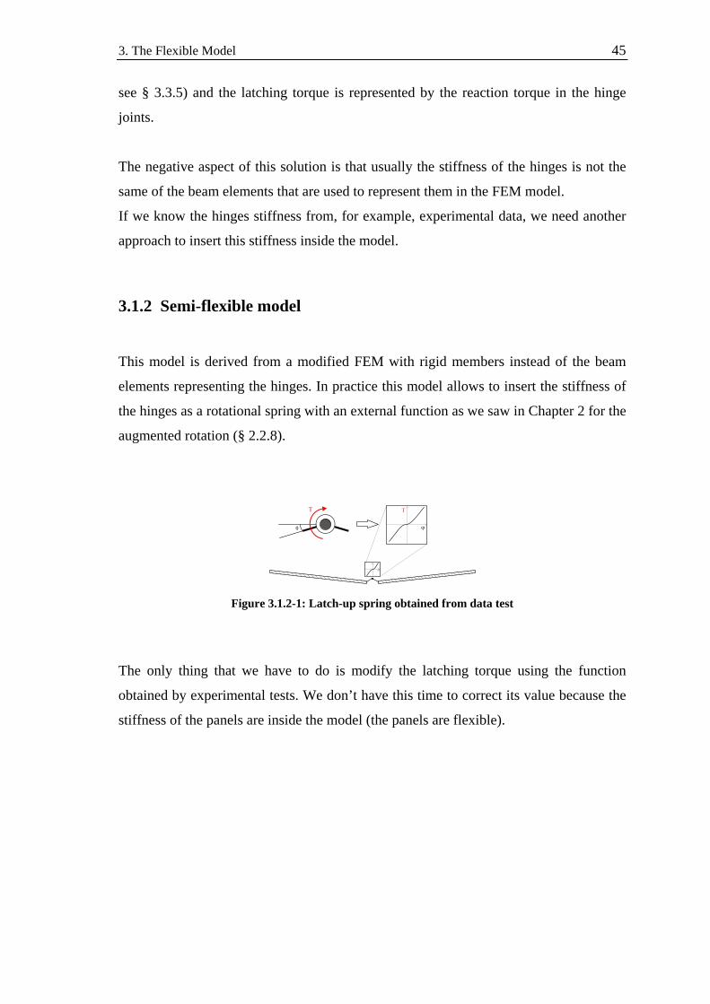
3. The Flexible Model 45
see § 3.3.5) and the latching torque is represented by the reaction torque in the hinge
joints.
The negative aspect of this solution is that usually the stiffness of the hinges is not the
same of the beam elements that are used to represent them in the FEM model.
If we know the hinges stiffness from, for example, experimental data, we need another
approach to insert this stiffness inside the model.
3.1.2 Semi-flexible model
This model is derived from a modified FEM with rigid members instead of the beam
elements representing the hinges. In practice this model allows to insert the stiffness of
the hinges as a rotational spring with an external function as we saw in Chapter 2 for the
augmented rotation (§ 2.2.8).
Figure 3.1.2-1: Latch-up spring obtained from data test
The only thing that we have to do is modify the latching torque using the function
obtained by experimental tests. We don’t have this time to correct its value because the
stiffness of the panels are inside the model (the panels are flexible).

3. The Flexible Model 46
3.2 Generation of Flexible bodies
The flexible parts will be generated using the NASTRAN – ADAMS interface of
NASTRAN.
All the information (model stiffness, mass and loads matrixes, nodes location, mass
invariants) are stored in one single file for each flexible body created, a Modal Neutral
File (MNF). For the theory behind this interface one can refers to Chapter 1.
For what concern the generation of the MNF file and how to import them in ADAMS
please refer to the Appendixes 2 and 4.
The three fundamental aspects that have to be taken in consideration during the
generation of a flexible body are
1. The definition of the Attachment Points and their DOF
2. The choice of the number of dynamic modes (fix-interface normal modes)
3. Generation of PLOTEL elements grid
While the meaning of the first two points is clear from Chapter 1 point 3 introduces a
new aspect that will be further explained in paragraph 3.2.3.
It is clear that the bigger the number of fix-interface modes and of APs’ DOF is the
better is the approximation of the behaviour of the flexible body.
On the other hand, if we increase the number of modes that describe the body, we
increase the dimensions of the several matrixes involved in the solution of the problem
and so the complexity of the numerical resolution.
From there, we look for a method that lets us to catch the essence of the flexible body
using a minimum number of modes.
The number of modes will depend on the objective of our analysis. If we are interested
in a frequency-response analysis or in a latching torque evaluation it’s clear that we will
have to consider different numbers of modes.

3. The Flexible Model 47
The default number of fix-interface modes to pass to ADAMS in the NASTRAN-
ADAMS interface is 26 while, regarding the DOF of the APs, the MSC advice is to
consider all the 6 DOFs in a 3D problem.
modes fix-interface DOF modes 26 6i i i
i iN N n AP N AP= + ⋅ ⎯⎯→ = + ⋅∑ ∑
This number of modes doesn’t rise a problem when we deal with a single flexible body
in a rigid environment; but when we have to deal with a bigger number of flexible
bodies interacting each other, this yields a heavy numerical burden with a high number
of DOF, many of which are useless for a dynamic analysis.

3. The Flexible Model 48
3.2.1 Definition of Attachment Points and of their DOF
As we have seen in the first chapter the definition of the Attachment Points (AP) is of
essential importance for capturing the effect of attachments on the flexible body. Their
definition is quite intuitive; one has to define an AP in every node of the body that is in
contact with other bodies, subjected to forces or displacements (for this reason an AP is
also called interface or boundary node) and for each AP selected the whole set of
relative DOF should be used. If we not consider all these 6 DOF, and so all the
constraint modes related to an AP, it has the effect of additional constraints in the model
and consequently, this may lead to converge and locking problems in the dynamic
analysis.
In our model this rule has always to be applied for the hinge nodes. However, an
exception can be made for the forces when we are not interested in their local effects. If
we don’t need a good resolution of the zone where the load is applied and if we are
interested only to its global effect we can avoid to define an AP and apply the load
directly on the simple node.
The aerodynamic loads on AMOS-3 on-ground models are an example of such a case;
we are interested only in the global effects of these loads and we can apply them in the
node closest to the centre of mass. Another example is shown in Figure 3.2.1-1. This
time too we don’t need to know the local effect of the concentrated torque on the yoke
(also because in reality is generated by two forces from the pulleys that bend the cable)
but we want to take into account its global effect (on the frictions for example) by
applying the torque to a simple node of the yoke.
On the other hand, in case of an impact analysis (see Chapter 6) we are interested in a
better local description and so we will define the node located on the impact point as an
AP.

3. The Flexible Model 49
Figure 3.2.1-1: Example of load applied on a simple node
When we define the APs for a semi-flexible model we have to pay attention to how we
define the RBE2 elements that make the hinges rigid. As shown in second part of
Figure 3.2.1-2 the AP node has always to be the independent node of an RBE2 element
otherwise we get an error during the generation of the MNF file.
Figure 3.2.1-2: Attachment point definition
For the same reason we can’t put more than one AP on the rigid part of a structure.
Figure 3.2.1-3 shows the rigid part of a yoke. Only the AP shown in the figure is
possible, the other nodes are dependent.
Figure 3.2.1-3: Attachment point in a rigid structure
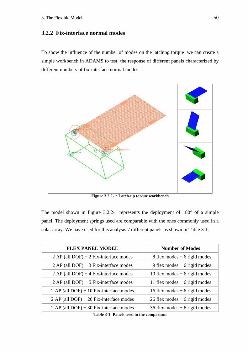
3. The Flexible Model 50
3.2.2 Fix-interface normal modes
To show the influence of the number of modes on the latching torque we can create a
simple workbench in ADAMS to test the response of different panels characterized by
different numbers of fix-interface normal modes.
Figure 3.2.2-1: Latch-up torque workbench
The model shown in Figure 3.2.2-1 represents the deployment of 180° of a simple
panel. The deployment springs used are comparable with the ones commonly used in a
solar array. We have used for this analysis 7 different panels as shown in Table 3-1.
FLEX PANEL MODEL Number of Modes
2 AP (all DOF) + 2 Fix-interface modes 8 flex modes + 6 rigid modes
2 AP (all DOF) + 3 Fix-interface modes 9 flex modes + 6 rigid modes
2 AP (all DOF) + 4 Fix-interface modes 10 flex modes + 6 rigid modes
2 AP (all DOF) + 5 Fix-interface modes 11 flex modes + 6 rigid modes
2 AP (all DOF) + 10 Fix-interface modes 16 flex modes + 6 rigid modes
2 AP (all DOF) + 20 Fix-interface modes 26 flex modes + 6 rigid modes
2 AP (all DOF) + 30 Fix-interface modes 36 flex modes + 6 rigid modes Table 3-1: Panels used in the comparison
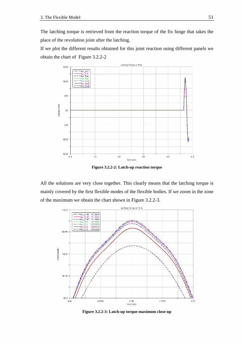
3. The Flexible Model 51
The latching torque is retrieved from the reaction torque of the fix hinge that takes the
place of the revolution joint after the latching.
If we plot the different results obtained for this joint reaction using different panels we
obtain the chart of Figure 3.2.2-2
Figure 3.2.2-2: Latch-up reaction torque
All the solutions are very close together. This clearly means that the latching torque is
mainly covered by the first flexible modes of the flexible bodies. If we zoom in the zone
of the maximum we obtain the chart shown in Figure 3.2.2-3.
Figure 3.2.2-3: Latch-up torque maximum close-up
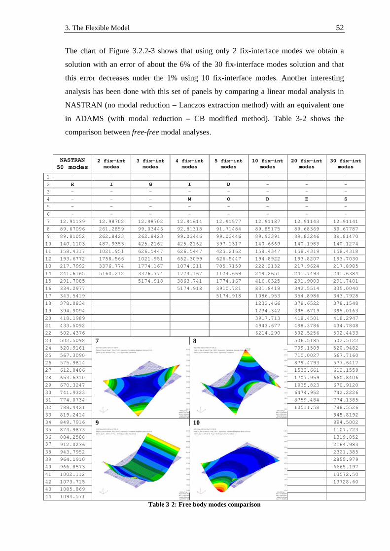
3. The Flexible Model 52
The chart of Figure 3.2.2-3 shows that using only 2 fix-interface modes we obtain a
solution with an error of about the 6% of the 30 fix-interface modes solution and that
this error decreases under the 1% using 10 fix-interface modes. Another interesting
analysis has been done with this set of panels by comparing a linear modal analysis in
NASTRAN (no modal reduction – Lanczos extraction method) with an equivalent one
in ADAMS (with modal reduction – CB modified method). Table 3-2 shows the
comparison between free-free modal analyses.
NASTRAN 50 modes
2 fix-int modes
3 fix-int modes
4 fix-int modes
5 fix-int modes
10 fix-int modes
20 fix-int modes
30 fix-int modes
1 - - - - - - - - 2 R I G I D - - - 3 - - - - - - - - 4 - - - M O D E S 5 - - - - - - - - 6 - - - - - - - - 7 12.91139 12.98702 12.98702 12.91614 12.91577 12.91187 12.91143 12.91141 8 89.67096 261.2859 99.03446 92.81318 91.71484 89.85175 89.68369 89.67787 9 89.81052 262.8423 262.8423 99.03446 99.03446 89.93391 89.83246 89.81470 10 140.1103 487.9353 425.2162 425.2162 397.1317 140.6669 140.1983 140.1274 11 158.4317 1021.951 626.5447 626.5447 425.2162 158.4347 158.4319 158.4318 12 193.6772 1758.566 1021.951 652.3099 626.5447 194.8922 193.8207 193.7030 13 217.7992 3376.774 1774.167 1074.211 705.7159 222.2132 217.9624 217.8985 14 241.6165 5160.212 3376.774 1774.167 1124.669 249.2651 241.7493 241.6384 15 291.7085 5174.918 3863.741 1774.167 416.0325 291.9003 291.7401 16 334.2977 5174.918 3910.721 831.8419 342.5514 335.0040 17 343.5419 5174.918 1086.953 354.8986 343.7928 18 378.0834 1232.466 378.6522 378.1548 19 394.9094 1234.342 395.6719 395.0163 20 418.1989 3917.713 418.4501 418.2947 21 433.5092 4943.677 498.3786 434.7848 22 502.4376 6214.290 502.5256 502.4433 23 502.5098 506.5185 502.5122 24 520.9161 709.1509 520.9482 25 567.3090 710.0027 567.7160 26 575.9814 879.4793 577.6417 27 612.0406 1533.661 612.1559 28 653.6310 1707.959 660.8406 29 670.3247 1935.823 670.9120 30 741.9323 6474.952 742.2226 31 774.0734 8759.484 774.1385 32 788.4421 10511.58 788.5526 33 819.2414
7 8
845.8192 34 849.7916 894.5002 35 874.9873 1107.723 36 884.2588 1319.852 37 912.0236 2164.983 38 943.7952 2321.385 39 964.1910 2855.979 40 966.8573 6665.197 41 1002.112 13572.50 42 1073.715 13728.60 43 1085.869 44 1094.571
9 10
Table 3-2: Free body modes comparison

3. The Flexible Model 53
The second analysis, Table 3-3, shows the results obtained if we fix the two hinges of
the panel (the 2 APs). Because of the fact that we fix the APs the results that we obtain
in ADAMS are the same that we observe in NASTRAN (the fix-interface modes are in
fact obtained fixing the DOF of the APs ).
NASTRAN
50 modes 2 fix-int
modes
3 fix-int
modes
4 fix-int
modes
5 fix-int
modes
10 fix-int
modes
20 fix-int
modes
30 fix-int
modes
1 4.103071 4.103071 4.103071 4.103071 4.103070 4.103070 4.103071 4.103071 2 9.523196 9.523195 9.523196 9.523197 9.523195 9.523195 9.523195 9.523197 3 54.19069 54.19068 54.19068 54.19068 54.19070 54.19070 54.19070 4 69.25148 69.25147 69.25147 69.25148 69.25146 69.25147 5 97.80708 97.80714 97.80715 97.80714 97.80715 6 121.5842 121.5842 121.5842 121.5842 7 158.4196 158.4196 158.4196 158.4196 8 182.4240 182.4240 182.4240 182.4240 9 185.9918 185.9918 185.9918 185.9918 10 234.9154 234.9154 234.9154 234.9154 11 266.3860 266.3862 266.3862 12 287.8708 287.8716 287.8717 13 289.5280 289.5281 289.5281 14 322.2658 322.2658 322.2658 15 370.9318 370.9318 370.9318 16 396.3294 396.3294 396.3294 17 414.6130 414.6130 414.6130 18 502.5464 502.5466 502.5466 19 503.0186 503.0186 503.0186 20 513.7064 513.7104 5137.105 21 525.2734 525.2762 22 534.3716 534.3735 23 565.7713 565.7714 24 612.5683 612.5686 25 671.0543
1 2
671.0544 26 739.8488 739.8636 27 754.5557 754.5690 28 771.8421 771.8623 29 777.1147 777.1183 30 798.4374 798.4492 31 850.3492 32 899.0864 33 944.2161 34 963.4950 35 964.4594 36 973.8625
3 4
Table 3-3: Fix-interface modes comparation
One can conclude from the comparisons that for a good representation of the flexible
properties 10 fix-interface modes are a good compromise between results (latching
torque) and computational costs.
The same analysis can also be applied to the semi-flexible model. For the entity of the
latching spring stiffness we can use a tuned value to get similar torque magnitude as
with the pure flexible case.

3. The Flexible Model 54
Figure 3.2.2-4: Latching torque for a semi-flexible model
In the case of the semi-flexible model we see that the dependency of the lathing torque
with the number of fix-internal modes decreases significantly (Figure 3.2.2-4).
A number of 5 fix-interface modes are sufficient for the semi-flexible model.
At the end we can summarize all the choices to take in the following table
PURE – FLEXIBLE MODEL SEMI – FLEXIBLE MODEL
APs & their
DOF
All the interface nodes of the
flexible bodies with all the DOF
of the nodes
All the interface nodes of the
flexible bodies with all the DOF
of the nodes
Fix-interface
modes From 10 on From 5 on
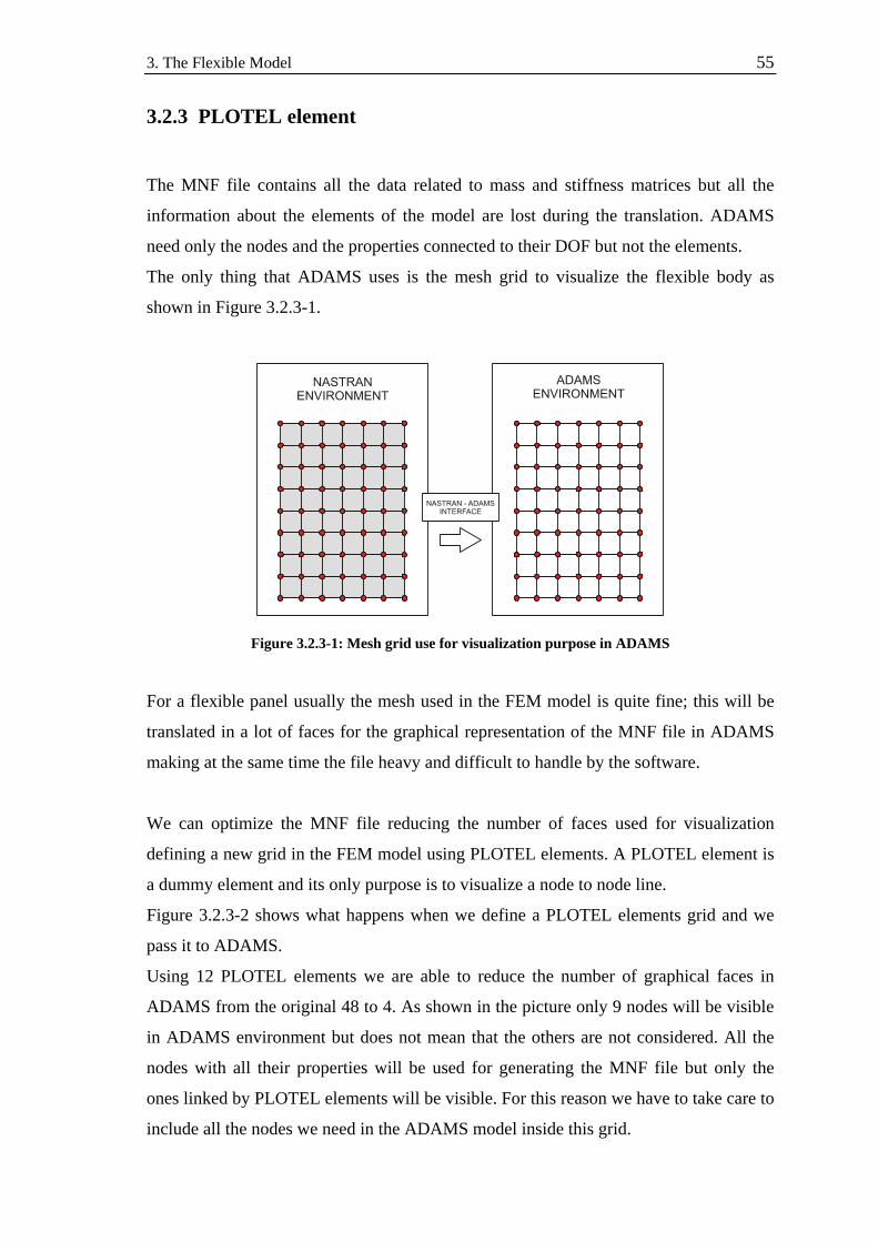
3. The Flexible Model 55
3.2.3 PLOTEL element
The MNF file contains all the data related to mass and stiffness matrices but all the
information about the elements of the model are lost during the translation. ADAMS
need only the nodes and the properties connected to their DOF but not the elements.
The only thing that ADAMS uses is the mesh grid to visualize the flexible body as
shown in Figure 3.2.3-1.
Figure 3.2.3-1: Mesh grid use for visualization purpose in ADAMS
For a flexible panel usually the mesh used in the FEM model is quite fine; this will be
translated in a lot of faces for the graphical representation of the MNF file in ADAMS
making at the same time the file heavy and difficult to handle by the software.
We can optimize the MNF file reducing the number of faces used for visualization
defining a new grid in the FEM model using PLOTEL elements. A PLOTEL element is
a dummy element and its only purpose is to visualize a node to node line.
Figure 3.2.3-2 shows what happens when we define a PLOTEL elements grid and we
pass it to ADAMS.
Using 12 PLOTEL elements we are able to reduce the number of graphical faces in
ADAMS from the original 48 to 4. As shown in the picture only 9 nodes will be visible
in ADAMS environment but does not mean that the others are not considered. All the
nodes with all their properties will be used for generating the MNF file but only the
ones linked by PLOTEL elements will be visible. For this reason we have to take care to
include all the nodes we need in the ADAMS model inside this grid.

3. The Flexible Model 56
Figure 3.2.3-2: PLOTEL elements grid used for visualization in ADAMS
There is not a particular strategy for creating the PLOTEL elements mesh. It is clear
that if we create a fine mesh we will have a better graphical result and a better
comprehension of the deformation shapes but we will pay this in terms of file size and
computational time.
When defining the PLOTEL lines one has to avoid the intersection between two or
more PLOTEL elements because this could generate misunderstanding. This situation is
well explained in the example of Figure 3.2.3-3 about a saddle deformation.
A square plane undergoes a
saddle deformation.
The intersection between
two PLOTEL elements generates
a bad deformation shape. The
saddle geometry is lost.
If we avoid the intersection
we obtain a better approximation
of the deformation shape.
Figure 3.2.3-3: Correct use of PLOTEL

3. The Flexible Model 57
It is clear that if we reduce the numbers of faces too much we will have a difficult
visualization in ADAMS; for example if we exaggerate the reduction this could make
modal shapes be difficult to understand and so on.
Even if the definition of the PLOTEL elements grid is possible in the PATRAN pre-
processor environment for the right working of the interface we have to modify few
strings of the BDF file generated before running NASTRAN. We have in fact to impose
manually that the PLOTEL elements grid has to be used for visualization purpose in
ADAMS.
For a more detailed tutorial about the PLOTEL elements generation please refer to
Appendix B.
Figure 3.2.3-4 shows the mesh reduction adopted for the MNF file of AMOS-3 solar
array panel 2. The reduced MNF file size is around 35 times smaller than the original
one!
Element Faces 2476 Element Faces 80
MNF File size 2537 KB MNF File size 72 KB Figure 3.2.3-4: File size reduction due to the use of PLOTEL elements
3. The Flexible Model 58
3.3 ADAMS flexible model
Once we have run the NASTRAN-ADAMS interface we obtain a MNF file for every
flexible bodies of our FEM model.
The next step at this point is to create a flexible dynamic model of the solar array
deployment.
Since the first step in the design of a solar array deployment model is an ADAMS rigid
model we can avoid to build a new model from the beginning and try to modify the
rigid one such that the flexible bodies can be imported easily. For this purpose we can
use a function in ADAMS/View that enables the user to replace a rigid body with is
flexible representation (refer to Appendix D).
The principal changes to apply to the ADAMS rigid model are reported in the following
list
• Split the forces and relocate them in their real application points
• Introducing auxiliary points
• Redefine markers dependencies
• Modify the kinds of hinges and friction
• Change from spring locking to kinematical locking (full-flexible only)
• Modify the ADAMS/solver script
3.3.1 Splitting forces and relocating them in their real application
points
In a rigid model there is no need to place the forces in their real application points along
the hinge line. One can simple put the global force due to the two deployment spring in
just one torque applied along the hinge line.
In the case of a flexible model instead we have to ensure that all the forces act in their
application points.
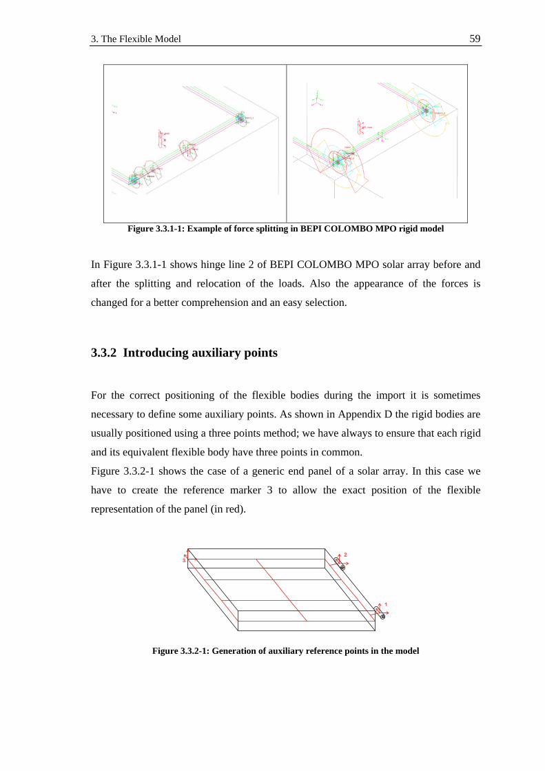
3. The Flexible Model 59
Figure 3.3.1-1: Example of force splitting in BEPI COLOMBO MPO rigid model
In Figure 3.3.1-1 shows hinge line 2 of BEPI COLOMBO MPO solar array before and
after the splitting and relocation of the loads. Also the appearance of the forces is
changed for a better comprehension and an easy selection.
3.3.2 Introducing auxiliary points
For the correct positioning of the flexible bodies during the import it is sometimes
necessary to define some auxiliary points. As shown in Appendix D the rigid bodies are
usually positioned using a three points method; we have always to ensure that each rigid
and its equivalent flexible body have three points in common.
Figure 3.3.2-1 shows the case of a generic end panel of a solar array. In this case we
have to create the reference marker 3 to allow the exact position of the flexible
representation of the panel (in red).
Figure 3.3.2-1: Generation of auxiliary reference points in the model
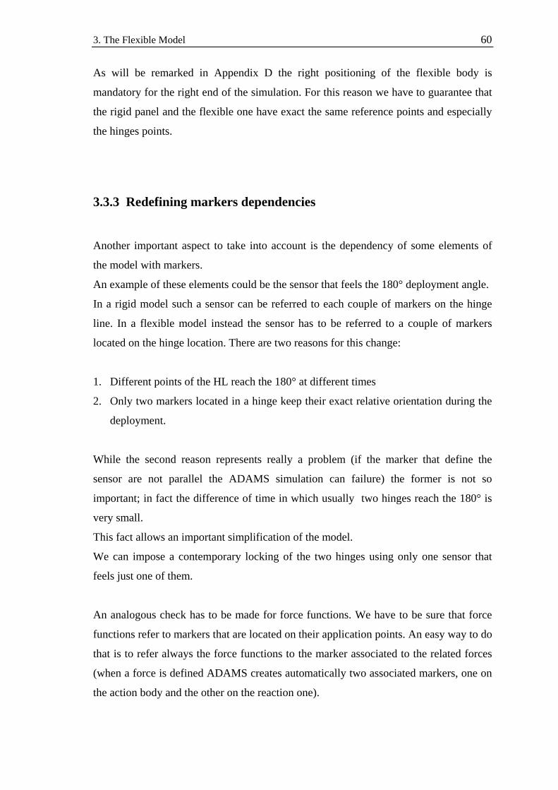
3. The Flexible Model 60
As will be remarked in Appendix D the right positioning of the flexible body is
mandatory for the right end of the simulation. For this reason we have to guarantee that
the rigid panel and the flexible one have exact the same reference points and especially
the hinges points.
3.3.3 Redefining markers dependencies
Another important aspect to take into account is the dependency of some elements of
the model with markers.
An example of these elements could be the sensor that feels the 180° deployment angle.
In a rigid model such a sensor can be referred to each couple of markers on the hinge
line. In a flexible model instead the sensor has to be referred to a couple of markers
located on the hinge location. There are two reasons for this change:
1. Different points of the HL reach the 180° at different times
2. Only two markers located in a hinge keep their exact relative orientation during the
deployment.
While the second reason represents really a problem (if the marker that define the
sensor are not parallel the ADAMS simulation can failure) the former is not so
important; in fact the difference of time in which usually two hinges reach the 180° is
very small.
This fact allows an important simplification of the model.
We can impose a contemporary locking of the two hinges using only one sensor that
feels just one of them.
An analogous check has to be made for force functions. We have to be sure that force
functions refer to markers that are located on their application points. An easy way to do
that is to refer always the force functions to the marker associated to the related forces
(when a force is defined ADAMS creates automatically two associated markers, one on
the action body and the other on the reaction one).
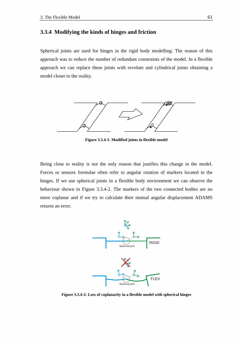
3. The Flexible Model 61
3.3.4 Modifying the kinds of hinges and friction
Spherical joints are used for hinges in the rigid body modelling. The reason of this
approach was to reduce the number of redundant constraints of the model. In a flexible
approach we can replace these joints with revolute and cylindrical joints obtaining a
model closer to the reality.
Figure 3.3.4-1: Modified joints in flexible model
Being close to reality is not the only reason that justifies this change in the model.
Forces or sensors formulae often refer to angular rotation of markers located in the
hinges. If we use spherical joints in a flexible body environment we can observe the
behaviour shown in Figure 3.3.4-2. The markers of the two connected bodies are no
more coplanar and if we try to calculate their mutual angular displacement ADAMS
returns an error.
Figure 3.3.4-2: Loss of coplanarity in a flexible model with spherical hinges

3. The Flexible Model 62
The change of joint types implies also a change in friction properties of the hinges.
Figure 3.3.4-3 shows how the friction properties were modified to get comparable result
between the two models for what concern the friction forces.
In a flexible model simulation a low value of the stiction transition velocity as the ones
showed can create some converge problems in the corrector formula of the integrator.
These problems usually happen in the very first instant of motion (when the model
starts moving) and can be avoided by increasing the value of this velocity by one order
of magnitude.
The resultant friction forces after these changes are close to the previous.
ADAMS spherical joint
(Rigid model) ADAMS revolute joint ADAMS cylindrical joint
Figure 3.3.4-3: Equivalent friction properties for different kinds of joints
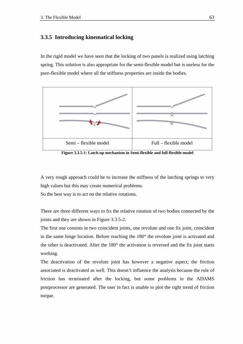
3. The Flexible Model 63
3.3.5 Introducing kinematical locking
In the rigid model we have seen that the locking of two panels is realized using latching
spring. This solution is also appropriate for the semi-flexible model but is useless for the
pure-flexible model where all the stiffness properties are inside the bodies.
Semi – flexible model Full – flexible model
Figure 3.3.5-1: Latch-up mechanism in Semi-flexible and full-flexible model
A very rough approach could be to increase the stiffness of the latching springs to very
high values but this may create numerical problems.
So the best way is to act on the relative rotations.
There are three different ways to fix the relative rotation of two bodies connected by the
joints and they are shown in Figure 3.3.5-2.
The first one consists in two coincident joints, one revolute and one fix joint, coincident
in the same hinge location. Before reaching the 180° the revolute joint is activated and
the other is deactivated. After the 180° the activation is reversed and the fix joint starts
working.
The deactivation of the revolute joint has however a negative aspect; the friction
associated is deactivated as well. This doesn’t influence the analysis because the role of
friction has terminated after the locking, but some problems in the ADAMS
postprocessor are generated. The user in fact is unable to plot the right trend of friction
torque.
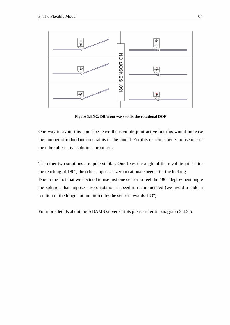
3. The Flexible Model 64
Figure 3.3.5-2: Different ways to fix the rotational DOF
One way to avoid this could be leave the revolute joint active but this would increase
the number of redundant constraints of the model. For this reason is better to use one of
the other alternative solutions proposed.
The other two solutions are quite similar. One fixes the angle of the revolute joint after
the reaching of 180°, the other imposes a zero rotational speed after the locking.
Due to the fact that we decided to use just one sensor to feel the 180° deployment angle
the solution that impose a zero rotational speed is recommended (we avoid a sudden
rotation of the hinge not monitored by the sensor towards 180°).
For more details about the ADAMS solver scripts please refer to paragraph 3.4.2.5.
3. The Flexible Model 65
3.3.6 Modifying the ADAMS/solver script
An ADAMS rigid body simulation is usually controlled by a user written script. The
commands are written in a particular language (e.g. ADAMS/solver language), that
describes the behaviour of model elements within the course of the simulation. It is easy
to divide the simulation in different phases, for example characterized by different time-
step control, or activate/deactivate options of forces or other elements in the model.
The scripted control enables also the user to select a particular integrator for the
equations of motion integrations. The default integrator, GSTIFF integrator, is the one
used for the rigid model simulations. This kind of integrator will be maintained also in
the flexible simulations.
The ADAMS/solver script used in the rigid simulation usually is not suitable for a
flexible simulation.
Besides the fact that forces ID are changed (due to the splitting and movements) and
new elements like locking devices are usually present when we pass to a flexible model
we have also to reconsider the different time stages of the simulation.
According to Chapter 1 it is clear that the numerical problem behind the flexible model
is more complex in comparison to rigid one. Besides the equations of motion, a system
of non-linear coupled differential and algebraic equations due to large displacements
and rotations during the deployment process, in a flexible model we have to deal with
bodies deformations and their modal representation.
For these reasons a first point to correct is the entity of integrator time-steps. If we want
to catch the effect of some high frequencies we have to decrease the integrator time-
step.
We can use the example used for the fix-interface modes (refer to paragraph 3.2.2) to
show the effect of different time steps on the latching torque.
Figure 3.3.6-1 shows the sensitivity of the latching torque due to variations of the
HMAX integrator parameter. HMAX defines the maximum time-step that the integrator
is allowed to take. There are no particular rules about how to choose the right value of
HMAX. The best way is to make different attempts and take the bigger one that
generates an accurate solution.

3. The Flexible Model 66
Figure 3.3.6-1: HMAX sensitiveness for full-flexible and semi-flexible model
Referring to the figure for example a good choice could be the solution
fm10_HMAX0001 generated by an HMAX 0.0001= .
It is always better not exceed in decreasing the time-step because the computational
times increase rapidly and mostly we can encounter corrector failures at small step
sizes. These occur because the Jacobian matrix is a function of the inverse of the step
size and becomes ill-conditioned at small steps.
Another way to modify the integrator time-step could be increase the number of output-
steps of the simulation. The output-step is the step that ADAMS use for plotting results
and HMAX is always smaller or equal to it.
Anyway is not advisable to use output-step smaller than the one necessary to have a
good graphical representation of results (the output files become uselessly big) so the
best procedure is to fix the right step for the output and then tune the model with
HMAX. Figure 3.3.6-2 shows the effects of different output-steps on the output.
Figure 3.3.6-2: Effect of different output-step on the plot of results

3. The Flexible Model 67
3.4 Applied Exemples
In the following paragraph we will show two examples of flexible modelling
• BEPI COLOMBO Mercury Polar Orbiter (MPO) solar array
• AMOS-3 solar array
- In orbit model
- On ground model
The flexible model will be obtained from the related rigid model (refer to paragraph
2.3). The following paragraphs report a brief explanation of the changes between the
two models. For more details about generation of flexible bodies or about how to import
them in ADAMS environment please refer to Appendix A and D.
3.4.1 BEPI COLOMBO MPO solar array – semi-flexible model
As first application example of the ADAMS flexible model will be considered the BEPI
COLOMBO MPO solar array.
As we have seen in Chapter 2 this solar array is composed by two panels and their
deployment is driven by a system of deployment springs.
Figure 3.4.1-1: BEPI COLOMBO MPO rigid and semi-flexible model
The flexible model will consist of two flexible panels as shown in Figure 3.4.1-1.
Since in this case we know the stiffness of the latched-up hinges on HL2 we will use a
semi-flexible model according to what said in paragraph 3.1.2. The beam elements that
represent the hinges on HL1 in the FEM will be included in the flexible body of panel 1.
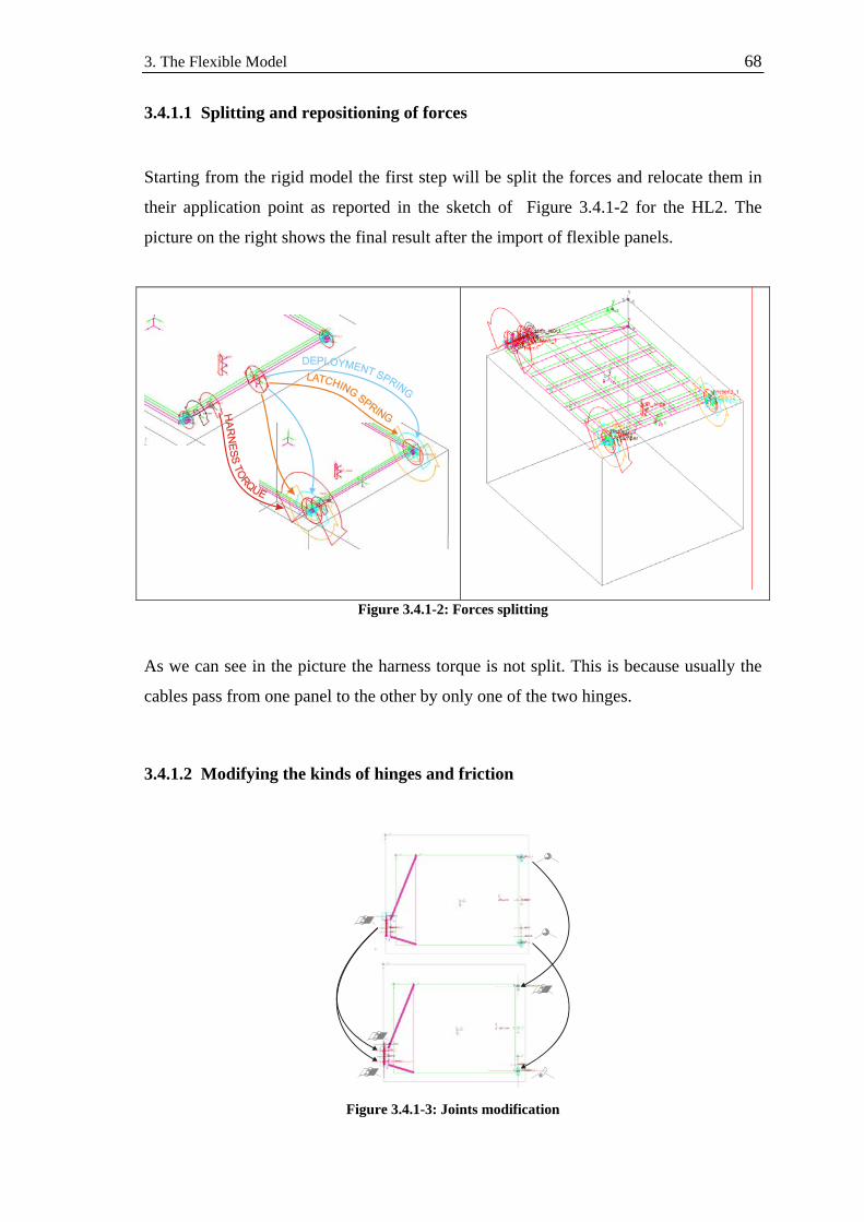
3. The Flexible Model 68
3.4.1.1 Splitting and repositioning of forces
Starting from the rigid model the first step will be split the forces and relocate them in
their application point as reported in the sketch of Figure 3.4.1-2 for the HL2. The
picture on the right shows the final result after the import of flexible panels.
Figure 3.4.1-2: Forces splitting
As we can see in the picture the harness torque is not split. This is because usually the
cables pass from one panel to the other by only one of the two hinges.
3.4.1.2 Modifying the kinds of hinges and friction
Figure 3.4.1-3: Joints modification
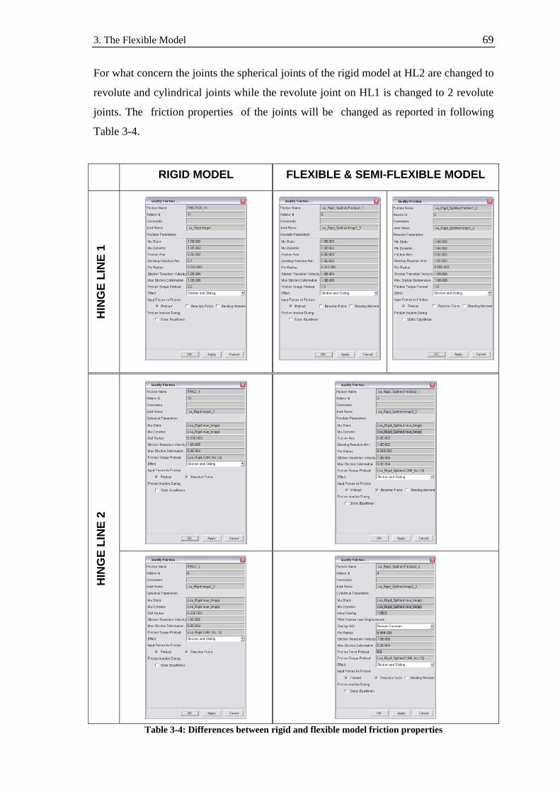
3. The Flexible Model 69
For what concern the joints the spherical joints of the rigid model at HL2 are changed to
revolute and cylindrical joints while the revolute joint on HL1 is changed to 2 revolute
joints. The friction properties of the joints will be changed as reported in following
Table 3-4.
RIGID MODEL FLEXIBLE & SEMI-FLEXIBLE MODEL
HIN
GE
LIN
E 1
HIN
GE
LIN
E 2
Table 3-4: Differences between rigid and flexible model friction properties
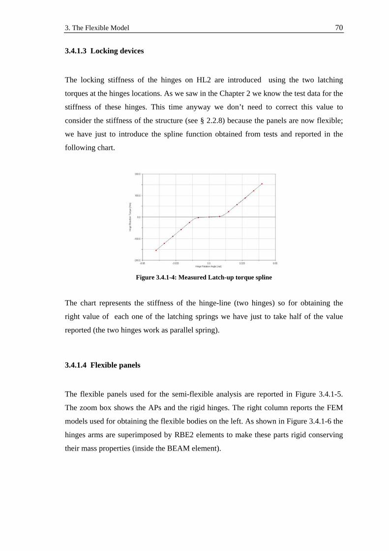
3. The Flexible Model 70
3.4.1.3 Locking devices
The locking stiffness of the hinges on HL2 are introduced using the two latching
torques at the hinges locations. As we saw in the Chapter 2 we know the test data for the
stiffness of these hinges. This time anyway we don’t need to correct this value to
consider the stiffness of the structure (see § 2.2.8) because the panels are now flexible;
we have just to introduce the spline function obtained from tests and reported in the
following chart.
Figure 3.4.1-4: Measured Latch-up torque spline
The chart represents the stiffness of the hinge-line (two hinges) so for obtaining the
right value of each one of the latching springs we have just to take half of the value
reported (the two hinges work as parallel spring).
3.4.1.4 Flexible panels
The flexible panels used for the semi-flexible analysis are reported in Figure 3.4.1-5.
The zoom box shows the APs and the rigid hinges. The right column reports the FEM
models used for obtaining the flexible bodies on the left. As shown in Figure 3.4.1-6 the
hinges arms are superimposed by RBE2 elements to make these parts rigid conserving
their mass properties (inside the BEAM element).

3. The Flexible Model 71
Figure 3.4.1-6: Rigid hinges obtained by RBE2 superimposition
We have 4 APs for panel1 and 2 APs for panel2. If we take 5 fix-interface modes we
obtain:
6 r-b modes
modes P1 FLEX modes P16 r-b modes
modes P2 FLEX modes P2
6 29 23
6
5
5 17 12 1
4N N
N N
−
−
= + ⋅ = ⎯⎯⎯⎯→ =
= + ⋅ = ⎯⎯⎯⎯→ =
Figure 3.4.1-5: BEPI COLOMBO MPO Flexible model characteristics
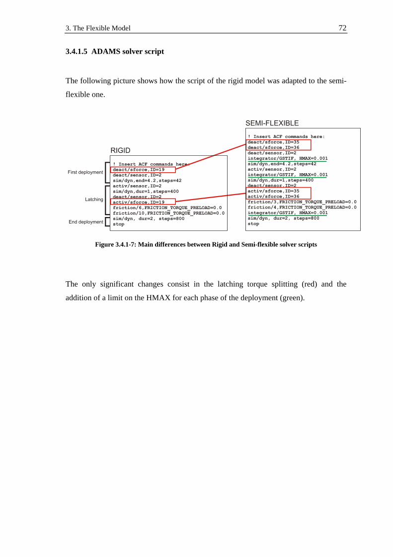
3. The Flexible Model 72
3.4.1.5 ADAMS solver script
The following picture shows how the script of the rigid model was adapted to the semi-
flexible one.
Figure 3.4.1-7: Main differences between Rigid and Semi-flexible solver scripts
The only significant changes consist in the latching torque splitting (red) and the
addition of a limit on the HMAX for each phase of the deployment (green).
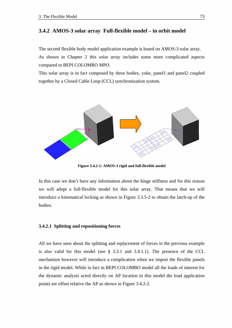
3. The Flexible Model 73
3.4.2 AMOS-3 solar array Full-flexible model – in orbit model
The second flexible body model application example is based on AMOS-3 solar array.
As shown in Chapter 2 this solar array includes some more complicated aspects
compared to BEPI COLOMBO MPO.
This solar array is in fact composed by three bodies, yoke, panel1 and panel2 coupled
together by a Closed Cable Loop (CCL) synchronization system.
Figure 3.4.2-1: AMOS-3 rigid and full-flexible model
In this case we don’t have any information about the hinge stiffness and for this reason
we will adopt a full-flexible model for this solar array. That means that we will
introduce a kinematical locking as shown in Figure 3.3.5-2 to obtain the latch-up of the
bodies.
3.4.2.1 Splitting and repositioning forces
All we have seen about the splitting and replacement of forces in the previous example
is also valid for this model (see § 3.3.1 and 3.4.1.1). The presence of the CCL
mechanism however will introduce a complication when we import the flexible panels
in the rigid model. While in fact in BEPI COLOMBO model all the loads of interest for
the dynamic analysis acted directly on AP location in this model the load application
points are offset relative the AP as shown in Figure 3.4.2-2.

3. The Flexible Model 74
Figure 3.4.2-2: Offset of CCL loads
The problem of the offset is due to the fact that the pulleys are not represented in the
FEM model and their mass is simple added to the mass of the hinges. This means when
we import the flexible bodies we don’t have a node to apply the loads on. This problem
can be solved preserving the location of the offset load relative to near hinge node (AP).
ADAMS will automatically generate the rigid link showed in Figure 3.4.2-2.
The same Figure shows also a load that acts on a simple node; it is the torque acting on
the yoke arm which results from the CCL guidance. The user in this case has simply to
manually select the node to apply the load on, otherwise ADAMS will apply the load to
the nearest AP.
For a better comprehension of the importing flexible bodies process please refer to
Appendix D. Figure 3.4.2-3 shows the final flexible model with split and relocated
forces.
Figure 3.4.2-3: AMOS-3 full-flexible model
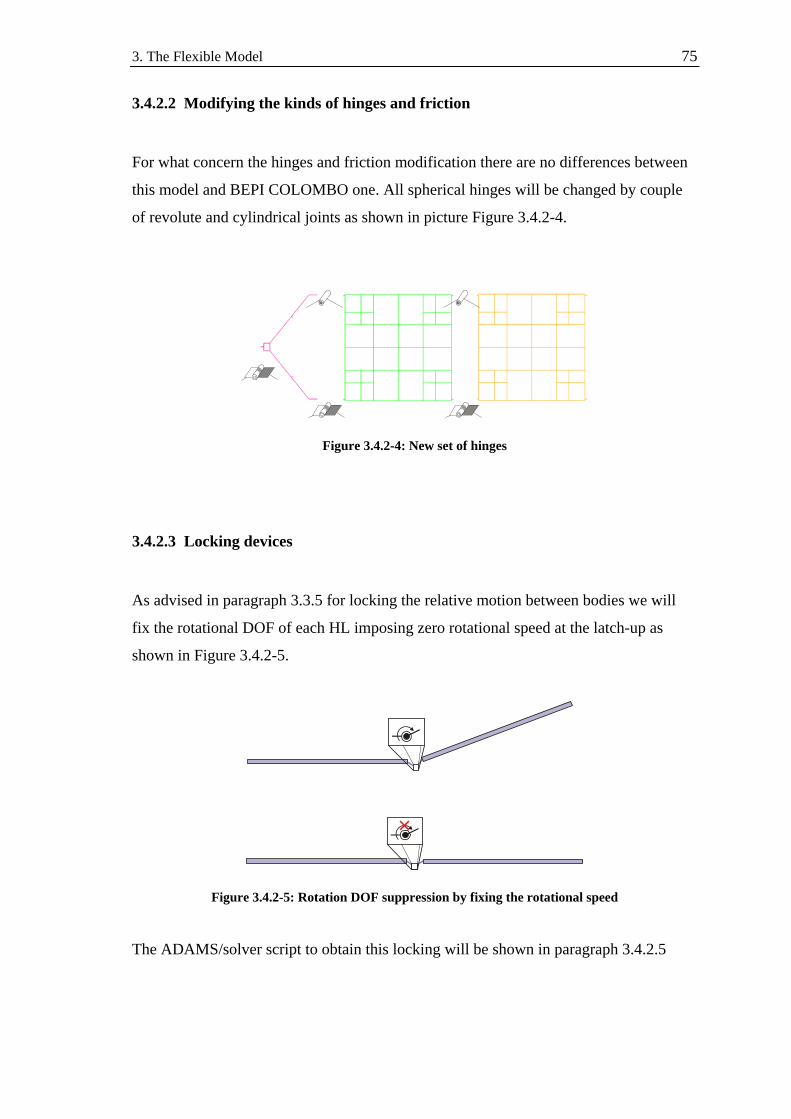
3. The Flexible Model 75
3.4.2.2 Modifying the kinds of hinges and friction
For what concern the hinges and friction modification there are no differences between
this model and BEPI COLOMBO one. All spherical hinges will be changed by couple
of revolute and cylindrical joints as shown in picture Figure 3.4.2-4.
Figure 3.4.2-4: New set of hinges
3.4.2.3 Locking devices
As advised in paragraph 3.3.5 for locking the relative motion between bodies we will
fix the rotational DOF of each HL imposing zero rotational speed at the latch-up as
shown in Figure 3.4.2-5.
Figure 3.4.2-5: Rotation DOF suppression by fixing the rotational speed
The ADAMS/solver script to obtain this locking will be shown in paragraph 3.4.2.5
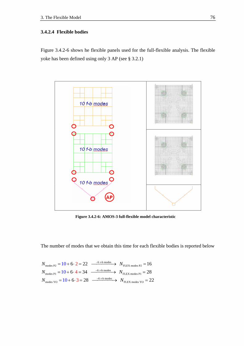
3. The Flexible Model 76
3.4.2.4 Flexible bodies
Figure 3.4.2-6 shows he flexible panels used for the full-flexible analysis. The flexible
yoke has been defined using only 3 AP (see § 3.2.1)
The number of modes that we obtain this time for each flexible bodies is reported below
Figure 3.4.2-6: AMOS-3 full-flexible model characteristic
6 r-b modesmodes P2 FLEX modes P2
6 r-b modesmodes P1 FLEX modes P1
6 r-b modesmodes YO FLEX modes YO
6 22 16
6 34 28
6 28 2
2
4
3
0
2
1
10
10
N N
N N
N N
−
−
−
= + ⋅ = ⎯⎯⎯⎯→ =
= + ⋅ = ⎯⎯⎯⎯→ =
= + ⋅ = ⎯⎯⎯⎯→ =

3. The Flexible Model 77
3.4.2.5 ADAMS solver script
The solver script has, compared to BEPI COLOMBO one, the particularity shown in
Figure 3.4.2-7. This time we don’t have to activate a torque but we define a new
ADAMS element, a MOTION, that we used to fix the rotational DOF of revolute and
cylindrical joints.
Figure 3.4.2-7: Full-flexible model script example

3. The Flexible Model 78
3.4.3 AMOS-3 solar array Full-flexible model – On ground model
The on-ground model of AMOS-3 solar array is shown in Figure 3.4.3-1.
Figure 3.4.3-1: AMOS-3 on-ground hybrid model
This model can be obtained in an analogous way as for the in-orbit one but there are
three different aspects that are useful to take in evidence.
• Aerodynamic load applied on simple nodes
• Support bracket represented as different bodies
• Coexistence of rigid and flexible parts in same model (hybrid-model)
3.4.3.1 Aerodynamic load applied on simple nodes
As we have already seen in early paragraph 3.2.1 we are interested only in aerodynamic
global effects. To consider the air drag that they generate, we can apply them to the
central node of each panel (the closer to the centre of mass) as shown in Figure 3.4.3-2

3. The Flexible Model 79
Figure 3.4.3-2: Aerodynamic loads on the panles
3.4.3.2 Support brackets represented as different bodies
The system of springs that compensates the gravitational forces on the structure is
connected to the panels and to the yoke by brackets. While in the rigid model we could
include their masses and their inertia properties inside the rigid body which they were
connected to, this time we have to consider them as separate entities.
Figure 3.4.3-3: Supporting brackets interfaces
Figure 3.4.3-3 shows the particular of the bracket. As we can see by the picture the
bracket is represented in ADAMS by a sphere of known mass rigidly connected to the
panel by a fix joint (the cyan padlocks of the picture on the right).
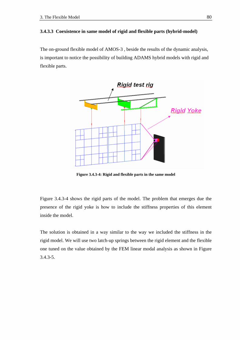
3. The Flexible Model 80
3.4.3.3 Coexistence in same model of rigid and flexible parts (hybrid-model)
The on-ground flexible model of AMOS-3 , beside the results of the dynamic analysis,
is important to notice the possibility of building ADAMS hybrid models with rigid and
flexible parts.
Figure 3.4.3-4: Rigid and flexible parts in the same model
Figure 3.4.3-4 shows the rigid parts of the model. The problem that emerges due the
presence of the rigid yoke is how to include the stiffness properties of this element
inside the model.
The solution is obtained in a way similar to the way we included the stiffness in the
rigid model. We will use two latch-up springs between the rigid element and the flexible
one tuned on the value obtained by the FEM linear modal analysis as shown in Figure
3.4.3-5.
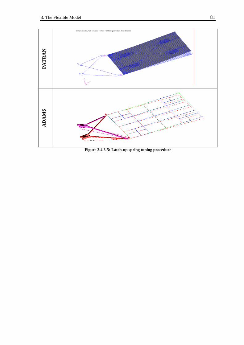
3. The Flexible Model 81
PAT
RA
N
AD
AM
S
Figure 3.4.3-5: Latch-up spring tuning procedure

Chapter 4 Analysis of Results
4.1 BEPI COLOMBO MPO S/A – Semi-flex vs Rigid Model
The following paragraph shows a comparison between the Semi-Flexible and Rigid
dynamic analyses of BEPI COLOMBO MPO solar array deployment.
4.1.1 Solar array Deployment
Sequence of Figure 4.1.1-1 shows the comparison between the deployments of the two
models. Even from the short sequence we can see how the two models are quite
synchronized. The deformation of bodies, as expected, doesn’t create any problem in
the flexible model.
The flexible model is the one on the right. As we can see by the sequence of pictures the
use of PLOTEL instead of the FEM mesh grid inhibits the rendering in ADAMS.
The colour-fringe plot present in the PLOTEL wire-frame during the deployment
indicates the magnitude of body deformation.
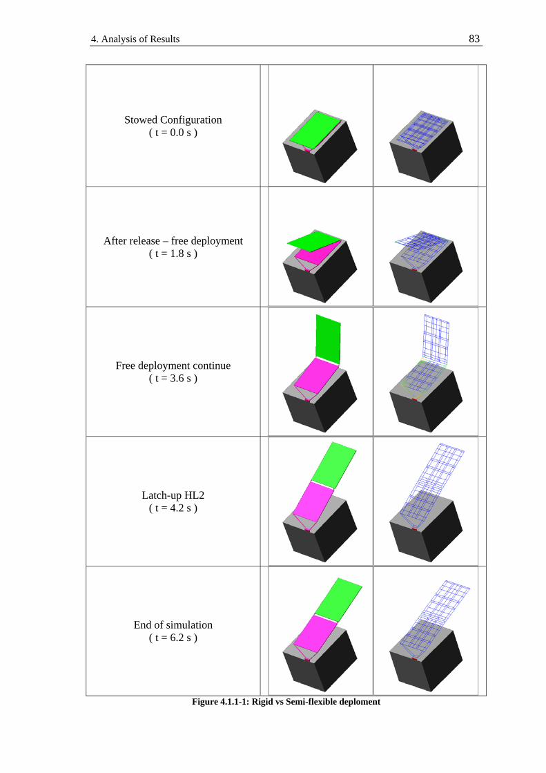
4. Analysis of Results 83
Stowed Configuration ( t = 0.0 s )
After release – free deployment ( t = 1.8 s )
Free deployment continue ( t = 3.6 s )
Latch-up HL2 ( t = 4.2 s )
End of simulation ( t = 6.2 s )
Figure 4.1.1-1: Rigid vs Semi-flexible deploment

4. Analysis of Results 84
4.1.2 Latch-up torque
The estimation of latch-up torque represents the main target of our investigation. Using
this torque in fact we are able to understand the entity of the loads associated with the
latching shock and find out the stress condition in the hinges surrounding areas.
Figure 4.1.2-1: Latch-up torque on HL2 Figure 4.1.2-1 show the latch-up torque vs time chart for the semi-flexible model. Top
left picture shows the starting time-step of the latch-up.
Even if the problem is slightly asymmetric (the two panels are different and the harness
torque involves only one hinge ) the two functions are in phase and the two maxima are
quite the same as shown in Errore. L'origine riferimento non è stata trovata.. In this
figure we can also recognize the flexibility from the non-linear experimental stiffness of
the hinges (refer to Figure 3.4.1-4).

4. Analysis of Results 85
Figure 4.1.2-2: Close up on the maximum latch-up torque
For comparing these results with the corresponding ones from the rigid model we have
to add the torque from the two hinges together since in the rigid model the latch-up
torque is represented by only one torque for the hinge-line.
Figure 4.1.2-3 shows this comparison.
Figure 4.1.2-3: Comparison between Rigid and Semi-flex model latch-up torque
The charts show that we have a good match between the results of the two models. The
rigid torque is characterized by a slightly higher peak value but that is not surprising
considering the approximation used to estimate the structural stiffness contribution of

4. Analysis of Results 86
the latch-up spring based only on the frequency of the first flexible mode of the
structure.
The small difference in the starting time of the latch-up (about 1 tenth of second) is due
to the imperfect equivalence of frictions of different joints (spherical vs revolute and
cylindrical) and to the differences in the integration steps between the two models. The
use of smaller integration time-step for the semi-flexible model leads to a more accurate
solution.
One more thing to notice is the different frequency of the oscillation. The lower
frequency of the semi-flexible is related with the lower stiffness of the model in
comparison with the rigid one.
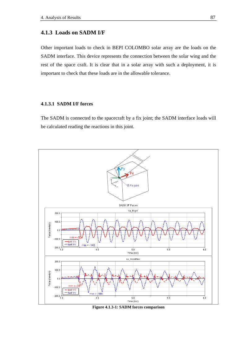
4. Analysis of Results 87
4.1.3 Loads on SADM I/F Other important loads to check in BEPI COLOMBO solar array are the loads on the
SADM interface. This device represents the connection between the solar wing and the
rest of the space craft. It is clear that in a solar array with such a deployment, it is
important to check that these loads are in the allowable tolerance.
4.1.3.1 SADM I/F forces
The SADM is connected to the spacecraft by a fix joint; the SADM interface loads will
be calculated reading the reactions in this joint.
Figure 4.1.3-1: SADM forces comparison

4. Analysis of Results 88
Figure 4.1.3-1 shows the comparison between rigid model result (upper chart) and semi-
flexible one (lower chart). As we can see also in this case the higher frequency effects
are quite restrained. The trend of the two forces is the same and the error on the
minimum value of yF is about 10%.
4.1.3.2 SADM I/F torques
From Figure 4.1.3-2 we can see that for the torques on the SADM interface the two
models show a quite different behaviour.
Figure 4.1.3-2: SADM torques comparison
The main difference is in the magnitude of yT . The rigid model underestimates the
magnitude of the torque around y by a factor of 1.77.

4. Analysis of Results 89
Beside this the trends of the curves, at least in a period of about 1 second after the latch-
up, are quite different and for the flexible result weakly periodic too.
This behaviour and these differences can be explained considering the asymmetry of the
structure of the solar array. The geometry and mass differences between the two panels
excite asymmetric flexible modes that can’t be captured with the 2 DOF approach of the
rigid model.

4. Analysis of Results 90
4.2 AMOS-3 S/A in orbit – Full-flex vs Rigid Model
4.2.1 Solar array Deployment
Stowed Configuration ( t = 0.0 s )
After release – free deployment ( t = 5.7 s )
Latch-up HL3 ( t = 7.5 s )
Latch-up HL2 ( t = 8.6 s )
Latch-up HL1 ( t =11.8 s )
Figure 4.2.1-1: Rigid vs Full-flexible deployment
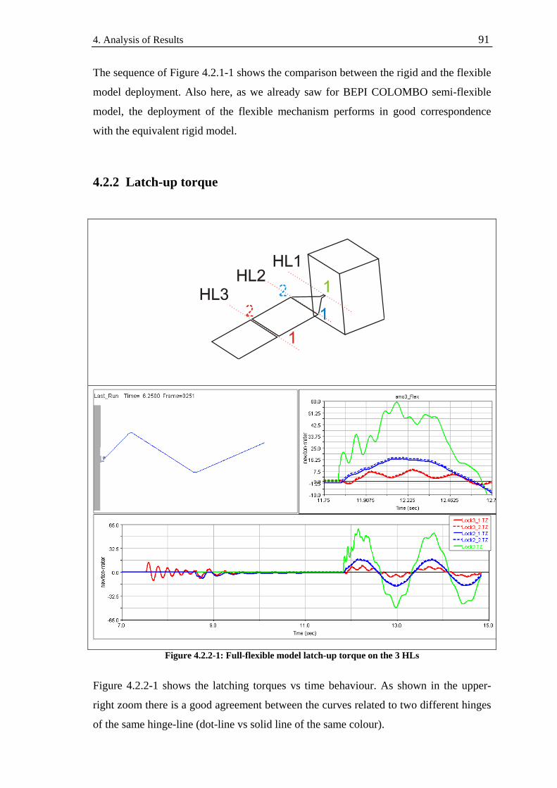
4. Analysis of Results 91
The sequence of Figure 4.2.1-1 shows the comparison between the rigid and the flexible
model deployment. Also here, as we already saw for BEPI COLOMBO semi-flexible
model, the deployment of the flexible mechanism performs in good correspondence
with the equivalent rigid model.
4.2.2 Latch-up torque
Figure 4.2.2-1: Full-flexible model latch-up torque on the 3 HLs
Figure 4.2.2-1 shows the latching torques vs time behaviour. As shown in the upper-
right zoom there is a good agreement between the curves related to two different hinges
of the same hinge-line (dot-line vs solid line of the same colour).

4. Analysis of Results 92
In the following paragraphs these latch-up torques will be compared with the ones
obtained by the rigid model. The two torques of each hinge-line from the flexible model
are add together to be compared with the rigid latching torque.
4.2.2.1 HL3 latch-up
Figure 4.2.2-2: Comparison between Rigid and Full-flexible latch-up torque on HL3
Figure 4.2.2-2 shows the comparison between rigid and flexible latch-up torque on
HL3. The two evolutions are quite similar; the maxima and the timings are comparable.
4.2.2.2 HL2 latch-up
Figure 4.2.2-3: Comparison between Rigid and Full-flexible latch-up torque on HL2
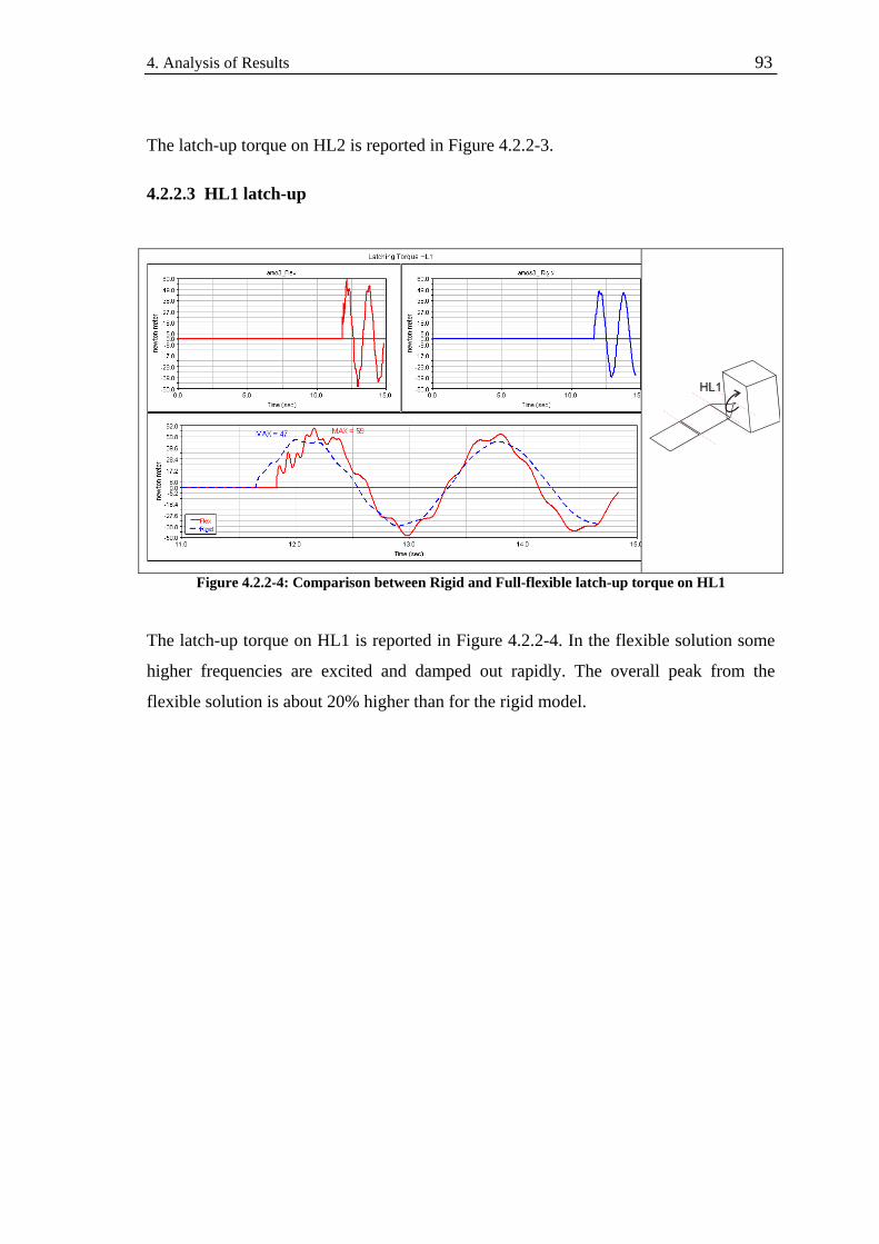
4. Analysis of Results 93
The latch-up torque on HL2 is reported in Figure 4.2.2-3.
4.2.2.3 HL1 latch-up
Figure 4.2.2-4: Comparison between Rigid and Full-flexible latch-up torque on HL1
The latch-up torque on HL1 is reported in Figure 4.2.2-4. In the flexible solution some
higher frequencies are excited and damped out rapidly. The overall peak from the
flexible solution is about 20% higher than for the rigid model.
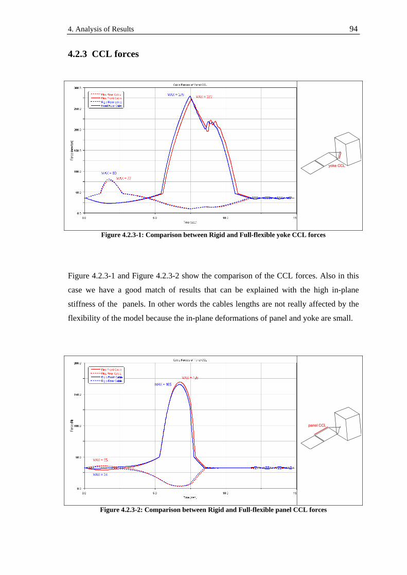
4. Analysis of Results 94
4.2.3 CCL forces
Figure 4.2.3-1: Comparison between Rigid and Full-flexible yoke CCL forces
Figure 4.2.3-1 and Figure 4.2.3-2 show the comparison of the CCL forces. Also in this
case we have a good match of results that can be explained with the high in-plane
stiffness of the panels. In other words the cables lengths are not really affected by the
flexibility of the model because the in-plane deformations of panel and yoke are small.
Figure 4.2.3-2: Comparison between Rigid and Full-flexible panel CCL forces

4. Analysis of Results 95
4.2.4 Eddy current dumper
Figure 4.2.4-1: Comparison between Rigid and Full-flexible eddy current damper torque
The behaviour of the resistive torque generated by the eddy current damper is reported
in Figure 4.2.4-1. The only relevant difference between the two models is after the
latching of HL1. After the latching of HL1 at about 12 [s]. We see that the rigid solution
keeps on oscillating around zero while the flexible solution goes straight to zero.
This difference is generated by the different latching devices used in the two models.
The locking spring of the rigid model enables the damper to work even after latch-up. In
the flexible model instead the relative rotation is fixed by the MOTION element (see
§3.3.5).

4. Analysis of Results 96
4.2.5 Torque on SADM I/F
The loads on the SADM are not critical for AMOS-3 solar array. Anyway we want to
warn the user about the problem of preload.
Figure 4.2.5-1 shows the Torque along y direction on the SADM I/F. As we can see in
the red square the first 4 seconds of the flexible simulation are characterized by a high
frequency oscillation. The reason for this behaviour is the lack of preload in the yoke.
ADAMS at the very first instant of simulation suddenly applies the set of CCL loads on
the yoke establishing that oscillation response shown in the picture.
The best solution to avoid this effect is to run a first static analysis fixing the hinge
DOF. This static simulation has only to load the yoke and after it we can start the
dynamic simulation with the preloaded yoke.
Figure 4.2.5-2 shows the same torque of Figure 4.2.5-1 obtained by a dynamic analysis
preceded by a static equilibrium in which we have fixed the HL DOF using the same
MOTION elements that will be used in the following dynamic analysis. The pick at
around second 12 is a numerical artefact generated by the latch-up of HL1; to fix it one
can decrease the time steps preceding the latch-up.
It is clear that the pre-load effects are not present in the rigid body (blue-dot line)
model.
Figure 4.2.5-1: Effect on the lack of preload on Yoke Ty torque
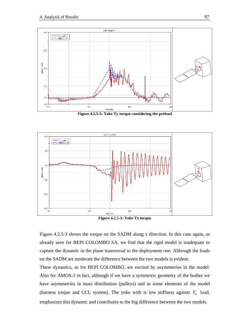
4. Analysis of Results 97
Figure 4.2.5-2: Yoke Ty torque considering the preload
Figure 4.2.5-3: Yoke Tx torque Figure 4.2.5-3 shows the torque on the SADM along x direction. In this case again, as
already seen for BEPI COLOMBO SA, we find that the rigid model is inadequate to
capture the dynamic in the plane transversal to the deployment one. Although the loads
on the SADM are moderate the difference between the two models is evident.
These dynamics, as for BEPI COLOMBO, are excited by asymmetries in the model.
Also for AMOS-3 in fact, although if we have a symmetric geometry of the bodies we
have asymmetries in mass distribution (pulleys) and in some elements of the model
(harness torque and CCL system). The yoke with is low stiffness against XT load,
emphasizes this dynamic and contributes to the big difference between the two models.
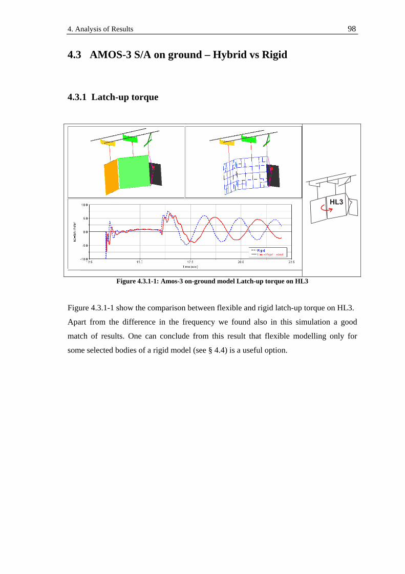
4. Analysis of Results 98
4.3 AMOS-3 S/A on ground – Hybrid vs Rigid
4.3.1 Latch-up torque
Figure 4.3.1-1: Amos-3 on-ground model Latch-up torque on HL3
Figure 4.3.1-1 show the comparison between flexible and rigid latch-up torque on HL3.
Apart from the difference in the frequency we found also in this simulation a good
match of results. One can conclude from this result that flexible modelling only for
some selected bodies of a rigid model (see § 4.4) is a useful option.

Chapter 5 Summary and Outlook
5.1 Rigid vs Flexible – Pro & Con of the two models
The comparison of analyses in Chapter 4 had shown a substantial good correlation
between the results of the two rigid and flexible (full & semi) models. Speaking about
the latch-up torque we have seen that the rigid is able to catch the essence of the
problem with the minimum number of DOF.
This fact demonstrates that the approximation of the latch-up stiffness in the rigid model
is essentially correct:
The latching torque is influenced mainly by the lowest bending mode of the two
structures involved in the latching, and the contributions of the other higher frequency
modes can be neglected.
Thanks to this result we are able to affirm that for the stress analysis of the structure in
NASTRAN a transient analysis is not mandatory. The low sensitivity of the latching
torque on the higher frequency dynamics of the structure will in fact allow us to

5. Summary and Outlook 100
represent the structural flexibility in a rotational spring with a stiffness value identified
from a simple modal analysis.
Anyway the flexible analysis has put in evidence some limitations of the rigid model.
As we have seen the rigid model can’t include higher frequency effects and, most of all,
can’t capture the dynamic effects outside the deployment plane as shown in Figure 5-1.
The rigid model represent a good approximation for the dynamics in the green plane of
the figure (latch-up torque) but we loose the flexible dynamic effects related to the other
two plane.
Figure 5-1: Deployment and transversal planes
So if we are interested in latch-up torque analysis this work has shown that the rigid
model approach is very good and that the flexible model solution represents only a
secondary improvement.
Otherwise, if we are interested in results that are influenced by transversal dynamics,
the flexible approach is advisable, mainly in those cases where we have important
asymmetries in the deployment plane.
The BEPI COLOMBO MPO example has shown that if we trust the rigid model we
have a torque on the SADM that is nearly half of the one obtained by the flexible
approach, and so the resulting margin of safety for that interface is strongly
overestimated.
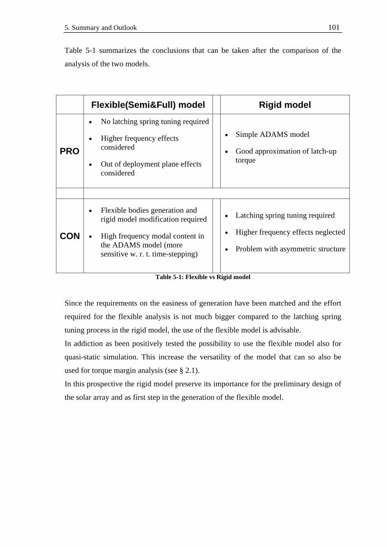
5. Summary and Outlook 101
Table 5-1 summarizes the conclusions that can be taken after the comparison of the
analysis of the two models.
Flexible(Semi&Full) model Rigid model
PRO
• No latching spring tuning required
• Higher frequency effects considered
• Out of deployment plane effects considered
• Simple ADAMS model
• Good approximation of latch-up torque
CON
• Flexible bodies generation and rigid model modification required
• High frequency modal content in the ADAMS model (more sensitive w. r. t. time-stepping)
• Latching spring tuning required
• Higher frequency effects neglected
• Problem with asymmetric structure
Table 5-1: Flexible vs Rigid model Since the requirements on the easiness of generation have been matched and the effort
required for the flexible analysis is not much bigger compared to the latching spring
tuning process in the rigid model, the use of the flexible model is advisable.
In addiction as been positively tested the possibility to use the flexible model also for
quasi-static simulation. This increase the versatility of the model that can so also be
used for torque margin analysis (see § 2.1).
In this prospective the rigid model preserve its importance for the preliminary design of
the solar array and as first step in the generation of the flexible model.

5. Summary and Outlook 102
5.2 Developments of Hybrid model
The result obtained by the hybrid model (see § 4.3) brings us to the conclusion that the
flexible approach, when necessary, can be restricted only to the parts of interest.
This will give us the option to study more complicated solar arrays restricting the
flexible analysis only on the bodies that, for example, are subjected to higher dynamic
load.
Figure 5-2: ARABSAT deployed configuration
A typical example suitable for this approach can be found in ARABSAT solar array.
This 6 bodies solar array (5 panels and yoke) is characterized by a first free spring
driven deployment of the first panel (see sequence of Figure 5-3 ) while all the others
are kept stowed.
Figure 5-3: ARABSAT first phase deployment
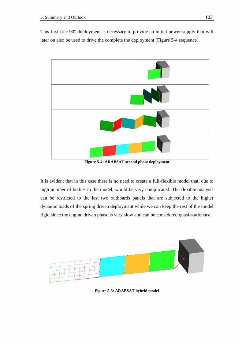
5. Summary and Outlook 103
This first free 90° deployment is necessary to provide an initial power supply that will
later on also be used to drive the complete the deployment (Figure 5-4 sequence).
Figure 5-4: ARABSAT second phase deployment
It is evident that in this case there is no need to create a full-flexible model that, due to
high number of bodies in the model, would be very complicated. The flexible analysis
can be restricted to the last two outboards panels that are subjected to the higher
dynamic loads of the spring driven deployment while we can keep the rest of the model
rigid since the engine driven phase is very slow and can be considered quasi-stationary.
Figure 5-5: ARABSAT hybrid model
Chapter 6 Alternative Fields of Application
6.1 Alternative application of the flexible approach
This chapter show two other possible fields of application of ADAMS/flex
• Stress & Strain in ADAMS environment
• Vibration Analysis
These two alternative applications need two plug-ins of ADAMS, ADAMS/Durability
for stress & strain evaluation and ADAMS/Vibration for vibration analyses.
6.1.1 Stress & Strain in ADAMS environment During the generation of flexible bodies in the NASTRAN – ADAMS interface we can
decide to include in the MNF file information concerning grid point stresses and strains.
We can use then this information to get an evaluation of stress & strain directly in
ADAMS environment.

6. Alternative Fields of Application 105
The grid point stress and strain information are determined by the related element
properties. So this time the FEM elements have a more important role then the merely
generation of a graphical grid for the flexible bodies visualization in ADAMS; the use
of the PLOTEL elements can anyway be useful as shown in Figure 6.1-1.
Figure 6.1-1: Stress visualization in a loaded rod with three different approaches
The three rods of Figure 6.1-1 show three different approaches to the problem.
The first flexible body on the left contains stress information for each grid point of the
FEM mesh. The middle one solution instead stores stress information only about the
middle part of the rod but anyway the total mesh grid is used for visualization purpose
in ADAMS. The last one is the solution obtained by the use of PLOTEL and, with the
same stress results as for other solution, is able to minimize the file size of the MNF
file.
3.6 MB 2.4 MB 0.9 MB
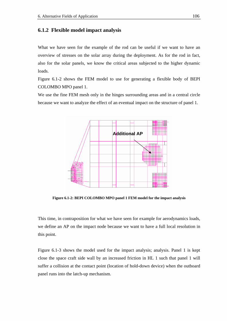
6. Alternative Fields of Application 106
6.1.2 Flexible model impact analysis What we have seen for the example of the rod can be useful if we want to have an
overview of stresses on the solar array during the deployment. As for the rod in fact,
also for the solar panels, we know the critical areas subjected to the higher dynamic
loads.
Figure 6.1-2 shows the FEM model to use for generating a flexible body of BEPI
COLOMBO MPO panel 1.
We use the fine FEM mesh only in the hinges surrounding areas and in a central circle
because we want to analyze the effect of an eventual impact on the structure of panel 1.
Figure 6.1-2: BEPI COLOMBO MPO panel 1 FEM model for the impact analysis
This time, in contraposition for what we have seen for example for aerodynamics loads,
we define an AP on the impact node because we want to have a full local resolution in
this point.
Figure 6.1-3 shows the model used for the impact analysis; analysis. Panel 1 is kept
close the space craft side wall by an increased friction in HL 1 such that panel 1 will
suffer a collision at the contact point (location of hold-down device) when the outboard
panel runs into the latch-up mechanism.
Additional AP

6. Alternative Fields of Application 107
Figure 6.1-3: Impact and hot spot stress analysis
The two right charts show the evolution of Von Mises stresses in the hot spot node (red
point below the right hinge in the picture) and in the impact node, respectively.
In this analysis we see that the impact is not critical with respect to the latch-up since
the maximum of the stress related to the latter is one order of magnitude bigger than the
one related to the former.
The user as to be aware that this stress analysis is anyway quite coarse and not sufficient
for a real stress analysis. In other words ADAMS\Durability does not substitute the
stress analysis in NASTRAN but anyway it can be useful in the design of the solar array
deployment to see how different choices influence directly the stresses.
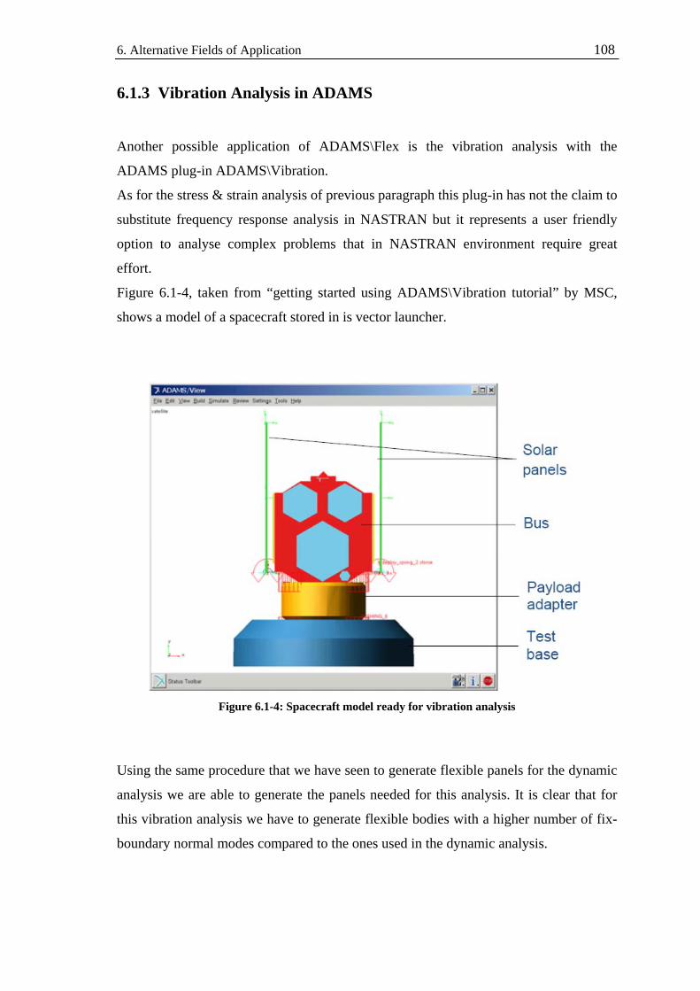
6. Alternative Fields of Application 108
6.1.3 Vibration Analysis in ADAMS Another possible application of ADAMS\Flex is the vibration analysis with the
ADAMS plug-in ADAMS\Vibration.
As for the stress & strain analysis of previous paragraph this plug-in has not the claim to
substitute frequency response analysis in NASTRAN but it represents a user friendly
option to analyse complex problems that in NASTRAN environment require great
effort.
Figure 6.1-4, taken from “getting started using ADAMS\Vibration tutorial” by MSC,
shows a model of a spacecraft stored in is vector launcher.
Figure 6.1-4: Spacecraft model ready for vibration analysis
Using the same procedure that we have seen to generate flexible panels for the dynamic
analysis we are able to generate the panels needed for this analysis. It is clear that for
this vibration analysis we have to generate flexible bodies with a higher number of fix-
boundary normal modes compared to the ones used in the dynamic analysis.

6. Alternative Fields of Application 109
In ADAMS environment we are able for example to study a whole structure of a space-
craft using different flexible bodies for each subgroup of the structure.
Figure 6.1-5 shows the example of GAIA space-craft. For each subgroup on the left we
can generate an MNF file and then reassemble the spacecraft in ADAMS environment.
This let us for example to define for each flexible body a particular damping function.
The same picture shows also another important aspect. The payload can be represented
also by a super-element. Often the payload FEM model is available only in terms of a
super-element model or directly the MNF file of the payload (since each of them is just
a condensed model from which is impossible to go back to the generating FEM model).
Using ADAMS the spacecraft designer can generate the related MNF from the super-
element of the payload and include it in the ADAMS model and has the complete model
ready for modal analysis.
Figure 6.1-5: Generation of an ADAMS model using different flexible sub-groups
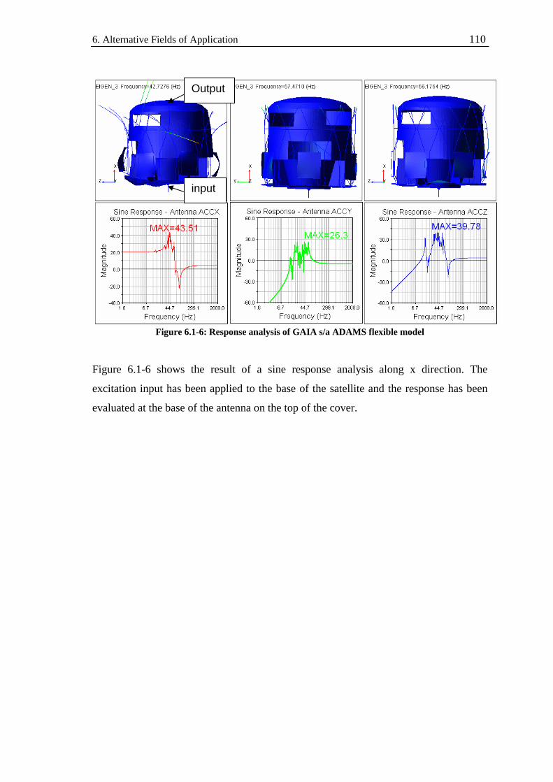
6. Alternative Fields of Application 110
Figure 6.1-6: Response analysis of GAIA s/a ADAMS flexible model
Figure 6.1-6 shows the result of a sine response analysis along x direction. The
excitation input has been applied to the base of the satellite and the response has been
evaluated at the base of the antenna on the top of the cover.
input
Output

Appendixes
The following appendixes represent some practical guides and tutorials in ADAMS and
PATRAN/NASTRAN environment. The appendixes will show some practical aspects
introduced in the first conceptual part.
The software version used in these tutorials are:
MSC.ADAMS 2005 r2
MSC.PATRAN 2005 r2
MSC.NASTRAN 2005

Appendix A Latch-up spring Tuning
The following tutorial explains how to use ADAMS to tune the latch-up spring of the rigid
model. This tuning process can be performed also in PATRAN (using BUSH element to
simulate the spring DOF at the HL) but the ADAMS way is easier and more intuitive.
The target for this condensation is that the first mode of two systems, one rigid with only 1
DOF (rotational along the hinge line) and the other flexible, has the same frequency for the
first deformation mode.
With this choice we implicitly assume that the flexibility effects are mainly due to the first
flex bending mode of the two bodies involved in the latch-up.
The following tutorial is based on BEPI COLOMBO MPO solar array.
A.1 Getting data from NASTRAN The first step of the tuning process is a modal linear analysis in NASTRAN. This analysis
will give us the frequency to use for tuning the springs in ADAMS. The normal modes
analysis has to be run with a model consisting of two bodies connected by the HL. These
two bodies are panel1 and panel2 for the BEPI COLOMBO example.
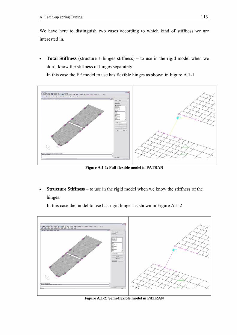
A. Latch-up spring Tuning 113
We have here to distinguish two cases according to which kind of stiffness we are
interested in.
• Total Stiffness (structure + hinges stiffness) – to use in the rigid model when we
don’t know the stiffness of hinges separately
In this case the FE model to use has flexible hinges as shown in Figure A.1-1
Figure A.1-1: Full-flexible model in PATRAN • Structure Stiffness – to use in the rigid model when we know the stiffness of the
hinges.
In this case the model to use has rigid hinges as shown in Figure A.1-2
Figure A.1-2: Semi-flexible model in PATRAN
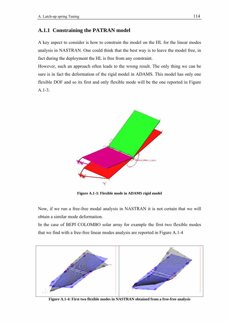
A. Latch-up spring Tuning 114
A.1.1 Constraining the PATRAN model A key aspect to consider is how to constrain the model on the HL for the linear modes
analysis in NASTRAN. One could think that the best way is to leave the model free, in
fact during the deployment the HL is free from any constraint.
However, such an approach often leads to the wrong result. The only thing we can be
sure is in fact the deformation of the rigid model in ADAMS. This model has only one
flexible DOF and so its first and only flexible mode will be the one reported in Figure
A.1-3.
Figure A.1-3: Flexible mode in ADAMS rigid model
Now, if we run a free-free modal analysis in NASTRAN it is not certain that we will
obtain a similar mode deformation.
In the case of BEPI COLOMBO solar array for example the first two flexible modes
that we find with a free-free linear modes analysis are reported in Figure A.1-4
Figure A.1-4: First two flexible modes in NASTRAN obtained from a free-free analysis
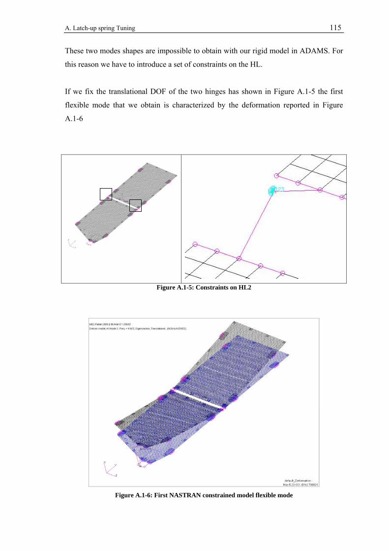
A. Latch-up spring Tuning 115
These two modes shapes are impossible to obtain with our rigid model in ADAMS. For
this reason we have to introduce a set of constraints on the HL.
If we fix the translational DOF of the two hinges has shown in Figure A.1-5 the first
flexible mode that we obtain is characterized by the deformation reported in Figure
A.1-6
Figure A.1-5: Constraints on HL2
Figure A.1-6: First NASTRAN constrained model flexible mode
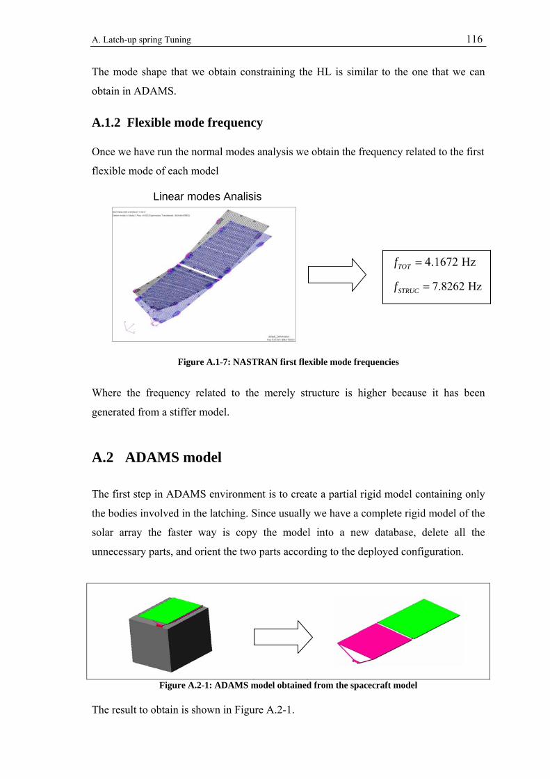
A. Latch-up spring Tuning 116
The mode shape that we obtain constraining the HL is similar to the one that we can
obtain in ADAMS.
A.1.2 Flexible mode frequency Once we have run the normal modes analysis we obtain the frequency related to the first
flexible mode of each model
Figure A.1-7: NASTRAN first flexible mode frequencies
Where the frequency related to the merely structure is higher because it has been
generated from a stiffer model.
A.2 ADAMS model
The first step in ADAMS environment is to create a partial rigid model containing only
the bodies involved in the latching. Since usually we have a complete rigid model of the
solar array the faster way is copy the model into a new database, delete all the
unnecessary parts, and orient the two parts according to the deployed configuration.
Figure A.2-1: ADAMS model obtained from the spacecraft model The result to obtain is shown in Figure A.2-1.
4.1672 HzTOTf =
7.8262 HzSTRUCf =
Linear modes Analisis
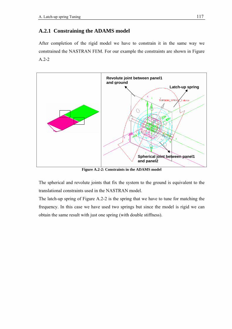
A. Latch-up spring Tuning 117
A.2.1 Constraining the ADAMS model After completion of the rigid model we have to constrain it in the same way we
constrained the NASTRAN FEM. For our example the constraints are shown in Figure
A.2-2
Figure A.2-2: Constraints in the ADAMS model
The spherical and revolute joints that fix the system to the ground is equivalent to the
translational constraints used in the NASTRAN model.
The latch-up spring of Figure A.2-2 is the spring that we have to tune for matching the
frequency. In this case we have used two springs but since the model is rigid we can
obtain the same result with just one spring (with double stiffness).
Spherical joint between panel1 and panel2
Latch-up spring
Revolute joint between panel1 and ground
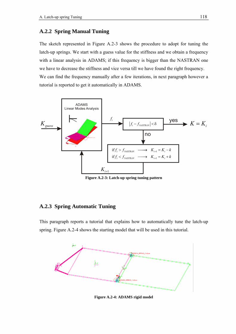
A. Latch-up spring Tuning 118
A.2.2 Spring Manual Tuning The sketch represented in Figure A.2-3 shows the procedure to adopt for tuning the
latch-up springs. We start with a guess value for the stiffness and we obtain a frequency
with a linear analysis in ADAMS; if this frequency is bigger than the NASTRAN one
we have to decrease the stiffness and vice versa till we have found the right frequency.
We can find the frequency manually after a few iterations, in next paragraph however a
tutorial is reported to get it automatically in ADAMS.
Figure A.2-3: Latch-up spring tuning pattern
A.2.3 Spring Automatic Tuning
This paragraph reports a tutorial that explains how to automatically tune the latch-up
spring. Figure A.2-4 shows the starting model that will be used in this tutorial.
Figure A.2-4: ADAMS rigid model

A. Latch-up spring Tuning 119
The constraints on hinges are shown in Figure A.2-2. The stiffness of the two springs
has to be defined as a design variable.
Select Build → Design Variable → New
We have to fill the box that appears as reported
in Figure A.2-5.
The unit for the stiffness is Nm/deg.
The range used is quite wide because we want to
be sure that the value we are looking for is
included.
Figure A.2-5
The next step is to assign this just created
variable as stiffness of the two springs as
reported in Figure A.2-6
Figure A.2-6
Now we have to perform a linear mode analysis using ADAMS\Vibration. If it is off
turn on the Vibration plug-in.
Select Tools → Plugin Manager → Load the ADAMS/Vibration by checking it Now a new Vibration menu should appear Select Vibration → Test → Vibration Analysis Fill the box that appears as shown in Figure A.2-7.
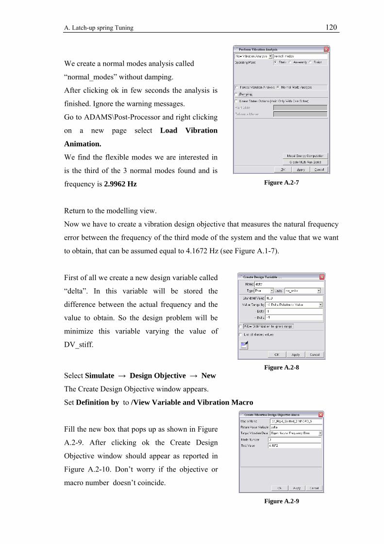
A. Latch-up spring Tuning 120
We create a normal modes analysis called
“normal_modes” without damping.
After clicking ok in few seconds the analysis is
finished. Ignore the warning messages.
Go to ADAMS\Post-Processor and right clicking
on a new page select Load Vibration
Animation.
We find the flexible modes we are interested in
is the third of the 3 normal modes found and is
frequency is 2.9962 Hz
Figure A.2-7
Return to the modelling view.
Now we have to create a vibration design objective that measures the natural frequency
error between the frequency of the third mode of the system and the value that we want
to obtain, that can be assumed equal to 4.1672 Hz (see Figure A.1-7).
First of all we create a new design variable called
“delta”. In this variable will be stored the
difference between the actual frequency and the
value to obtain. So the design problem will be
minimize this variable varying the value of
DV_stiff.
Figure A.2-8 Select Simulate → Design Objective → New
The Create Design Objective window appears.
Set Definition by to /View Variable and Vibration Macro
Fill the new box that pops up as shown in Figure
A.2-9. After clicking ok the Create Design
Objective window should appear as reported in
Figure A.2-10. Don’t worry if the objective or
macro number doesn’t coincide.
Figure A.2-9

A. Latch-up spring Tuning 121
Figure A.2-10
The next step is the creation of a multi-run vibration analysis script
Select Vibration → Test → Vibration Analysis
Select the Vibration analysis previously
created “normal_modes” and click on
Create Multi-Run Script button.
Leave the default values in the box that
appears and create the SIM_SCRIPT# by
clicking on ok.
Figure A.2-11 Now we are ready to run the optimization study
Select Simulate → Design Evaluation
The window of Figure A.2-12 will appear.
Select “DV_stiff” in the Design Variables
box. The Goal is minimize the
OBJECTIVE_3 previously created. Now
we can set up the Optimizer by clicking
on the corrisponding button. For this
analysis we can leave the default
tolerances and run the optimization
analysis by clicking on start.
Figure A.2-12
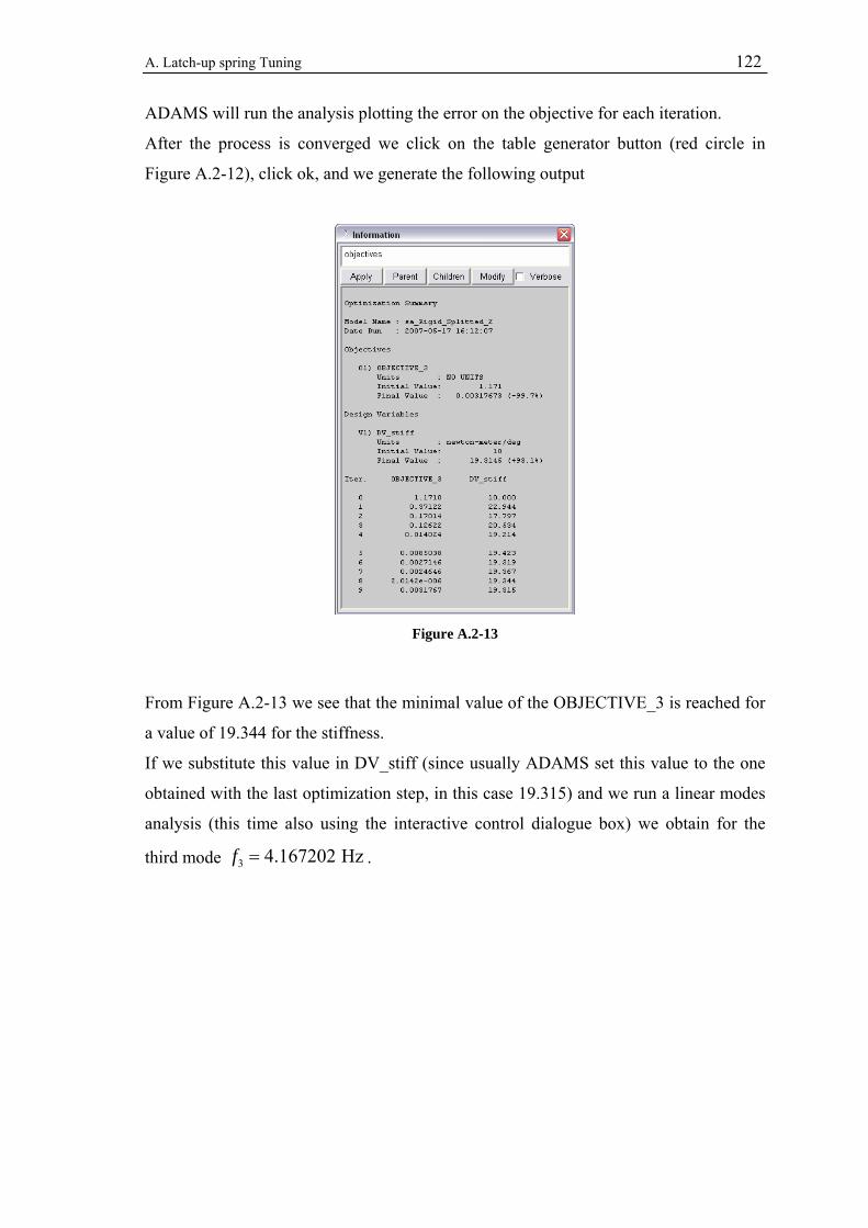
A. Latch-up spring Tuning 122
ADAMS will run the analysis plotting the error on the objective for each iteration.
After the process is converged we click on the table generator button (red circle in
Figure A.2-12), click ok, and we generate the following output
Figure A.2-13
From Figure A.2-13 we see that the minimal value of the OBJECTIVE_3 is reached for
a value of 19.344 for the stiffness.
If we substitute this value in DV_stiff (since usually ADAMS set this value to the one
obtained with the last optimization step, in this case 19.315) and we run a linear modes
analysis (this time also using the interactive control dialogue box) we obtain for the
third mode 3 4.167202 Hzf = .
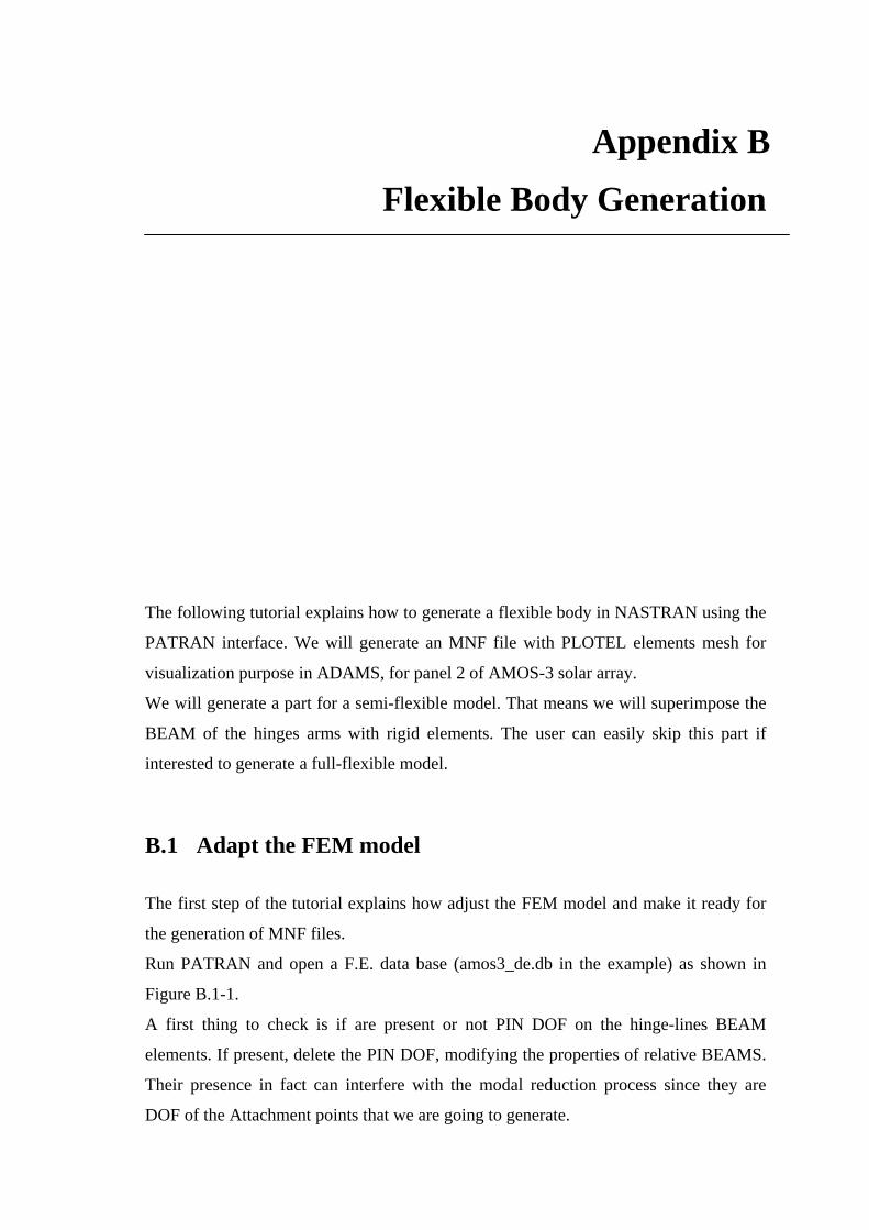
Appendix B Flexible Body Generation
The following tutorial explains how to generate a flexible body in NASTRAN using the
PATRAN interface. We will generate an MNF file with PLOTEL elements mesh for
visualization purpose in ADAMS, for panel 2 of AMOS-3 solar array.
We will generate a part for a semi-flexible model. That means we will superimpose the
BEAM of the hinges arms with rigid elements. The user can easily skip this part if
interested to generate a full-flexible model.
B.1 Adapt the FEM model
The first step of the tutorial explains how adjust the FEM model and make it ready for
the generation of MNF files.
Run PATRAN and open a F.E. data base (amos3_de.db in the example) as shown in
Figure B.1-1.
A first thing to check is if are present or not PIN DOF on the hinge-lines BEAM
elements. If present, delete the PIN DOF, modifying the properties of relative BEAMS.
Their presence in fact can interfere with the modal reduction process since they are
DOF of the Attachment points that we are going to generate.

B. Flexible Body Generation 124
Figure B.1-1: AMOS-3 FEM model
B.1.1 Rigid hinges and mass splitting
Select the group corresponding to the panel 2
Group…
Post… panel2 Apply
Create a new group called panel2_r. The letter r stands for rigid, that is because we will
substitute the beams that represent the local hinge stiffness property with rigid elements
(in the ADAMS model the flexibility of the hinges will be covered by the latching
spring)

B. Flexible Body Generation 125
Group…
Create…
New group name “panel2_r”
Entity selection “…all entities of panel2 group” Apply
Now we are ready to create the RBE rigid elements. In addition one has to set the point
masses located in the hinge center point to half of the corresponding hinges masses.
That is because just half of the hinge mass is associated to one panel.
Element ID 122389 Elmen props hmp1-2_1 Mass 0.0975
Element ID 140013 Elmen props conm2 Mass 0.195
Figure B.1-2: Hinges masses split between the two panels
Element
Action: Create Object: MPC Type: RBE2
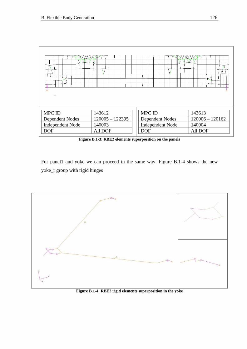
B. Flexible Body Generation 126
MPC ID 143612 Dependent Nodes 120005 – 122395 Independent Node 140003 DOF All DOF
MPC ID 143613 Dependent Nodes 120006 – 120162 Independent Node 140004 DOF All DOF
Figure B.1-3: RBE2 elements superposition on the panels
For panel1 and yoke we can proceed in the same way. Figure B.1-4 shows the new
yoke_r group with rigid hinges
Figure B.1-4: RBE2 rigid elements superposition in the yoke

B. Flexible Body Generation 127
B.1.2 Attachment Points definition
The further step will be the definition of the attachment points (APs). The APs and their
DOF define the generation of the constrained modes in the Craig-Bampton´s modal
reduction method (see Chapter 1).
The APs are all the interface nodes, in which two different bodies, in our example the
hinge node of two panels or of the first panel and the yoke, exchange forces and
torques. We will activate all 6 DOFs. This choice is not mandatory but if we not
consider all their DOF, and so all the constraint modes connected to an AP, it should be
like add additional constraints to the model (see Chapter 1).
Element
Action: Create Object: DOF List DOF List name “AP_p2”
Define terms…
Node List 140003 140004 DOFs All DOFs
Apply
Cancel
Apply
One has to be aware of some special aspects regarding the definition of APs in HL1
(hinge line 1).
Since the two real hinges of HL1 are collocated in the ADAMS model in only one
revolute joint, one has to define only one relative AP with all 6 DOFs as outlined in
figure below
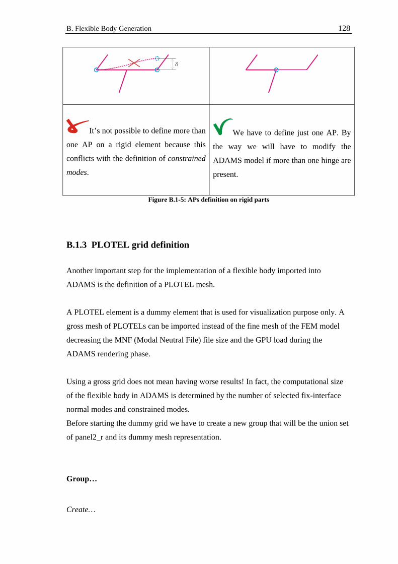
B. Flexible Body Generation 128
It’s not possible to define more than
one AP on a rigid element because this
conflicts with the definition of constrained
modes.
We have to define just one AP. By
the way we will have to modify the
ADAMS model if more than one hinge are
present.
Figure B.1-5: APs definition on rigid parts
B.1.3 PLOTEL grid definition
Another important step for the implementation of a flexible body imported into
ADAMS is the definition of a PLOTEL mesh.
A PLOTEL element is a dummy element that is used for visualization purpose only. A
gross mesh of PLOTELs can be imported instead of the fine mesh of the FEM model
decreasing the MNF (Modal Neutral File) file size and the GPU load during the
ADAMS rendering phase.
Using a gross grid does not mean having worse results! In fact, the computational size
of the flexible body in ADAMS is determined by the number of selected fix-interface
normal modes and constrained modes.
Before starting the dummy grid we have to create a new group that will be the union set
of panel2_r and its dummy mesh representation.
Group…
Create…
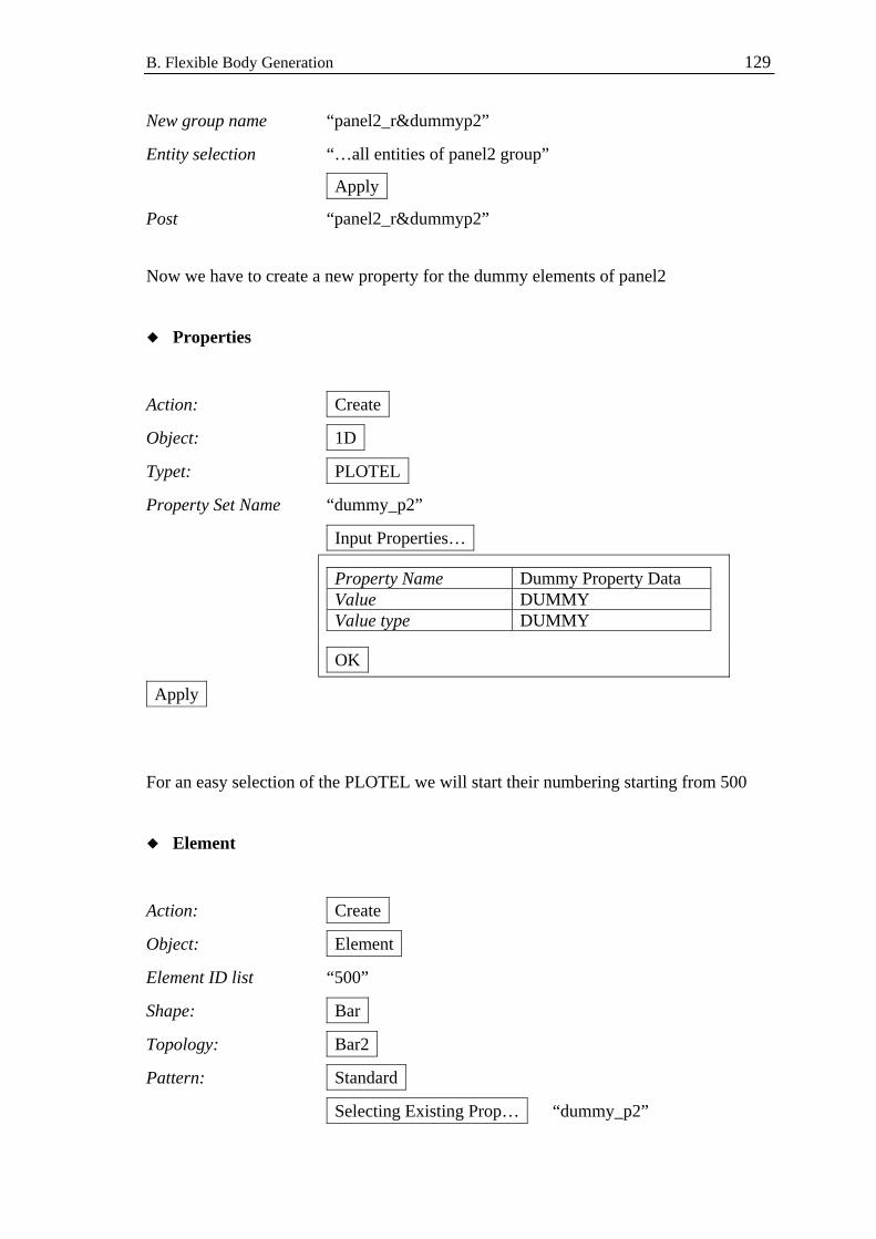
B. Flexible Body Generation 129
New group name “panel2_r&dummyp2”
Entity selection “…all entities of panel2 group”
Apply
Post “panel2_r&dummyp2”
Now we have to create a new property for the dummy elements of panel2
Properties
Action: Create Object: 1D Typet: PLOTEL Property Set Name “dummy_p2”
Input Properties…
Property Name Dummy Property Data Value DUMMY Value type DUMMY
OK
Apply
For an easy selection of the PLOTEL we will start their numbering starting from 500
Element
Action: Create Object: Element Element ID list “500”
Shape: Bar Topology: Bar2 Pattern: Standard Selecting Existing Prop… “dummy_p2”
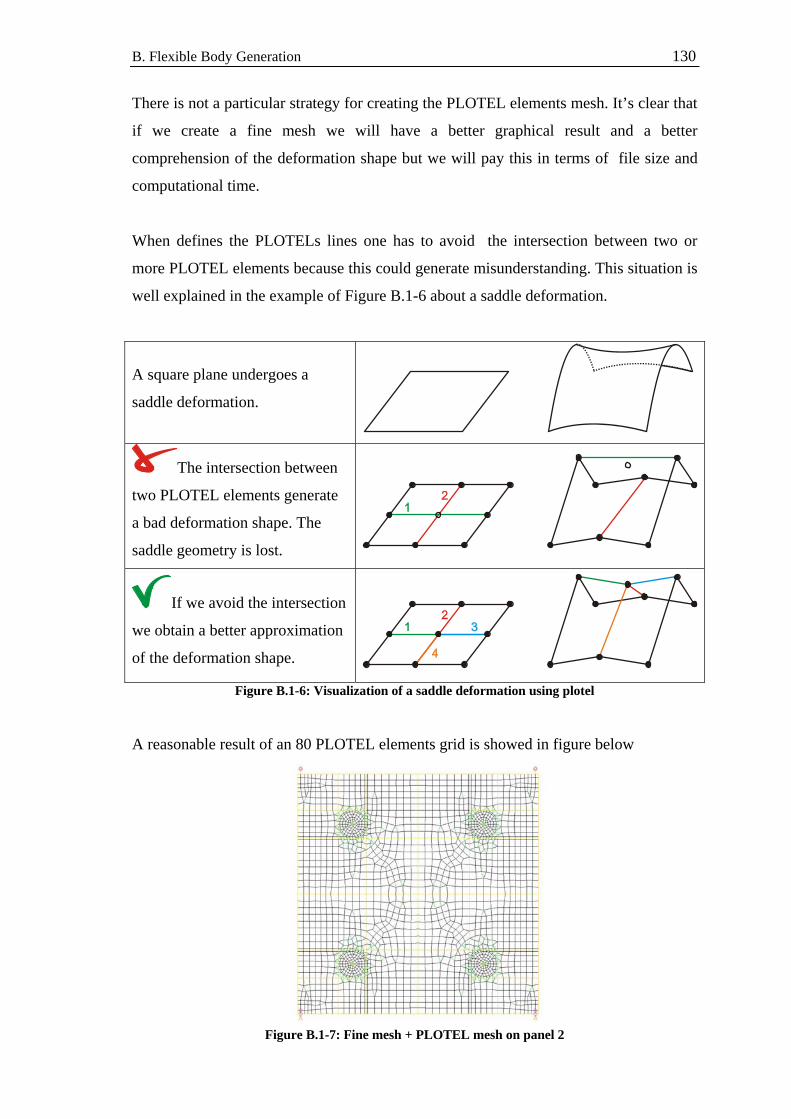
B. Flexible Body Generation 130
There is not a particular strategy for creating the PLOTEL elements mesh. It’s clear that
if we create a fine mesh we will have a better graphical result and a better
comprehension of the deformation shape but we will pay this in terms of file size and
computational time.
When defines the PLOTELs lines one has to avoid the intersection between two or
more PLOTEL elements because this could generate misunderstanding. This situation is
well explained in the example of Figure B.1-6 about a saddle deformation.
A square plane undergoes a
saddle deformation.
The intersection between
two PLOTEL elements generate
a bad deformation shape. The
saddle geometry is lost.
If we avoid the intersection
we obtain a better approximation
of the deformation shape.
Figure B.1-6: Visualization of a saddle deformation using plotel A reasonable result of an 80 PLOTEL elements grid is showed in figure below
Figure B.1-7: Fine mesh + PLOTEL mesh on panel 2

B. Flexible Body Generation 131
Now we can create a new group for the dummy grid
Group…
Create…
New group name “dummyp2”
Entity selection “Elm 500:579”
Apply
Post “dummyp2”
Figure B.1-8: PLOTEL mesh grid
Notice that for a correct working of the NASTRAN – ADAMS interface the nodes that
define the PLOTEL elements in the dummyp2 group have to be a subset of the nodes
from the fine mesh.

B. Flexible Body Generation 132
B.2 Definition of Load Cases
For creating the MNF to import in ADAMS we have to run a free-free modal analysis.
The related free-free load case without any forces or displacement is defined below.
Load Cases
Action: Create Load Case Name “free”
Input Data… …empty
B.3 Analysis
Now everything is prepared to go through the analysis phase. If we repeat the steps
before for each body of the solar array at this point we have the groups of Table B-1
ready for the analysis. We have now to run three different analyses, one for each of the
three bodies that form the solar array.
Group for the analyses Related PLOTEL mesh groups panel1_r&dummyp1 dummyp1 panel2_r&dummyp2 dummyp2 yoke_r&dummyyo dummyyo
Table B-1: Group for the analysis and related PLOTEL mesh group
Going on using panel 2
Action: Analyze Object: Selected Group Method: Analysis Deck Job Name “am3_p2_mnf”
Select Group…
panel2_r&dummyp2
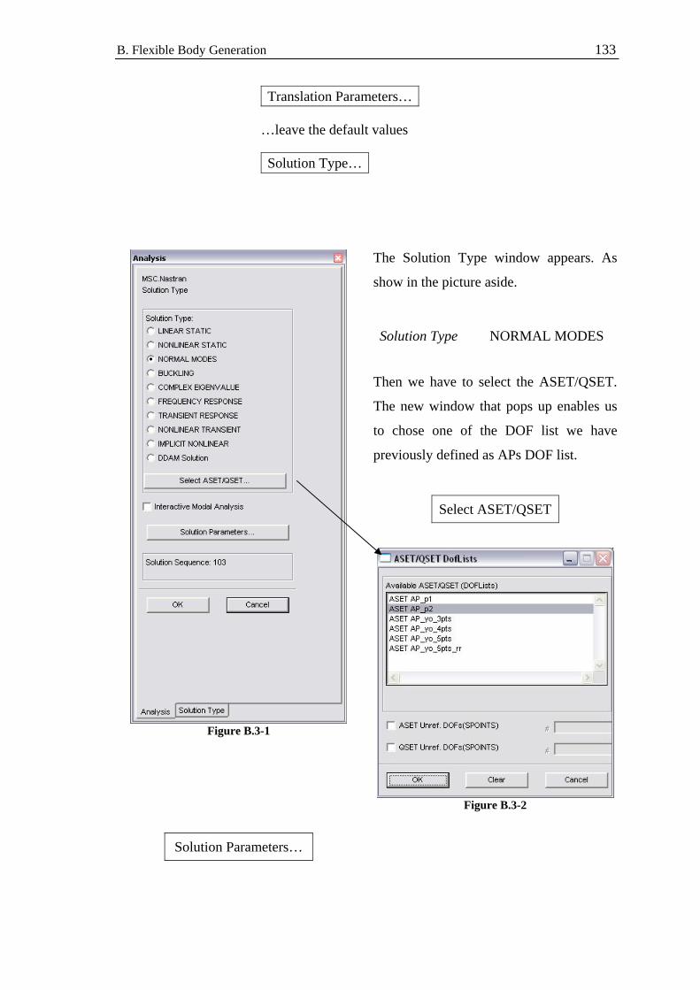
B. Flexible Body Generation 133
Translation Parameters…
…leave the default values
Solution Type…
Figure B.3-1
The Solution Type window appears. As
show in the picture aside.
Solution Type NORMAL MODES
Then we have to select the ASET/QSET.
The new window that pops up enables us
to chose one of the DOF list we have
previously defined as APs DOF list.
Select ASET/QSET
Figure B.3-2
Solution Parameters…

B. Flexible Body Generation 134
Figure B.3-3
Figure B.3-4
We can leave the default values show in the figure above and finally enter the ADAMS
Preparation menu.
ADAMS Output: MNF Only
In the ADAMS output there is also the option “Full Run + MNF” run which creates the
XDB file containing the modal results.
The modes that we obtain in this XDB file are those of the reduced model (Craig-
Bampton orthogonalized) and not those of the full F.E. model.
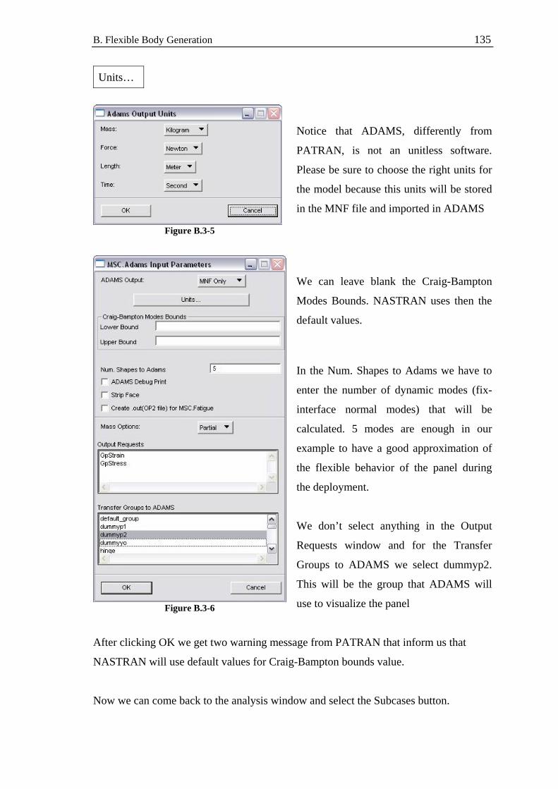
B. Flexible Body Generation 135
Figure B.3-5
Units…
Notice that ADAMS, differently from
PATRAN, is not an unitless software.
Please be sure to choose the right units for
the model because this units will be stored
in the MNF file and imported in ADAMS
We can leave blank the Craig-Bampton
Modes Bounds. NASTRAN uses then the
default values.
In the Num. Shapes to Adams we have to
enter the number of dynamic modes (fix-
interface normal modes) that will be
calculated. 5 modes are enough in our
example to have a good approximation of
the flexible behavior of the panel during
the deployment.
Figure B.3-6
We don’t select anything in the Output
Requests window and for the Transfer
Groups to ADAMS we select dummyp2.
This will be the group that ADAMS will
use to visualize the panel
After clicking OK we get two warning message from PATRAN that inform us that
NASTRAN will use default values for Craig-Bampton bounds value.
Now we can come back to the analysis window and select the Subcases button.
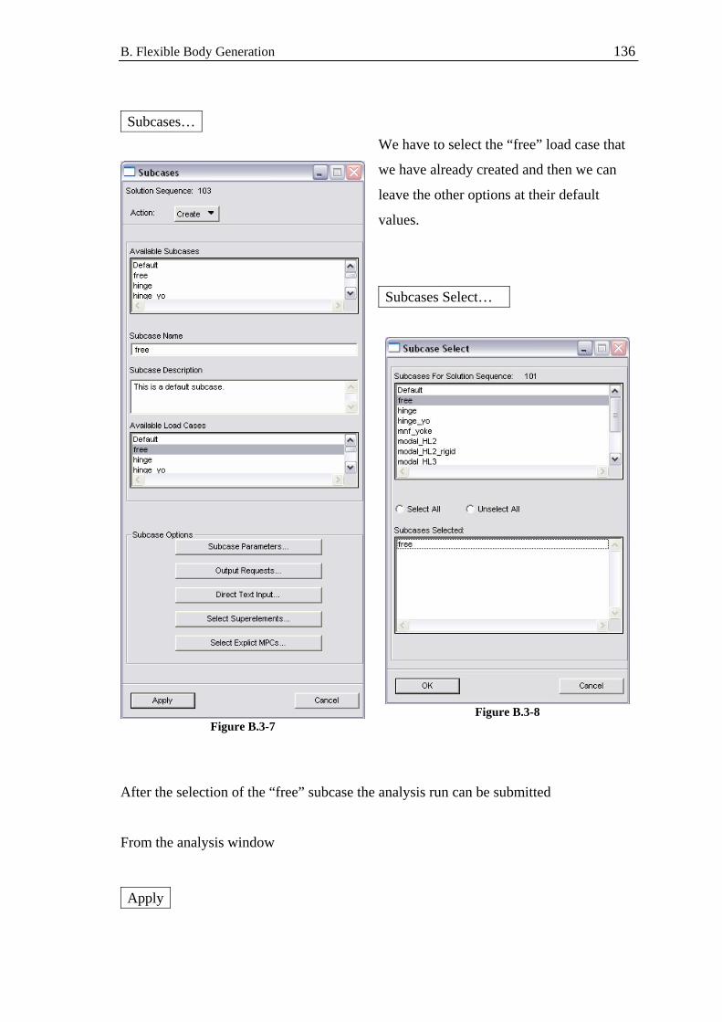
B. Flexible Body Generation 136
Figure B.3-7
Subcases…
We have to select the “free” load case that
we have already created and then we can
leave the other options at their default
values.
Figure B.3-8
Subcases Select…
After the selection of the “free” subcase the analysis run can be submitted
From the analysis window
Apply

B. Flexible Body Generation 137
PATRAN will create the .BDF input file for NASTRAN.
B.4 Editing the BDF file
The next step describes a manual adjustment to the BDF file. This change is necessary
because in the GUI of PATRAN is impossible to set the case control delimiter
OUTPUT with the input PLOT.
Figure B.4-1
PATRAN in fact set the OUTPUT
command to POST, but this is the command
for plotting grid pointes stresses or strains
even if they are not requested in the Output
Requests window as shown aside.
Instead we need OUTPUT(PLOT) which
introduces the plotter commands
responsible for the creation of the dummy
mesh used by ADAMS for visualization
purpose.
The strings reported in Figure B.4-2 show the simple change to apply at the BDF file

B. Flexible Body Generation 138
$ NASTRAN input file created by the MSC MSC.Nastran input file $ translator ( MSC.Patran 13.1.116 ) on January 16, 2007 at 14:51:46. $ Direct Text Input for Nastran System Cell Section $ Direct Text Input for File Management Section $ Normal Modes Analysis, Database SOL 103 $ Direct Text Input for Executive Control CEND TITLE = AMOS-3 SOLAR ARRAY ECHO = NONE SET 1=2 ADAMSMNF FLEXBODY=YES,FLEXONLY=YES,PSETID=1 $ Direct Text Input for Global Case Control Data SUBCASE 1 $ Subcase name : free SUBTITLE=free METHOD = 1 VECTOR(PLOT,SORT1,REAL)=ALL SPCFORCES(PLOT,SORT1,REAL)=ALL $ Direct Text Input for this Subcase OUTPUT(POST) $ Elements for group : dummyp2 SET 2 = 500 THRU 578,579 BEGIN BULK PARAM POST 0 PARAM SNORM 10. PARAM PRTMAXIM YES …
$NASTRAN input file created by the MSC MSC.Nastran input file $ translator ( MSC.Patran 13.1.116 ) on January 16, 2007 at 14:51:46. $ Direct Text Input for Nastran System Cell Section $ Direct Text Input for File Management Section $ Normal Modes Analysis, Database SOL 103 $ Direct Text Input for Executive Control CEND TITLE = AMOS-3 SOLAR ARRAY ECHO = NONE SET 1=2 ADAMSMNF FLEXBODY=YES,FLEXONLY=YES,PSETID=1 $ Direct Text Input for Global Case Control Data SUBCASE 1 $ Subcase name : free SUBTITLE=free METHOD = 1 VECTOR(PLOT,SORT1,REAL)=ALL SPCFORCES(PLOT,SORT1,REAL)=ALL $ Direct Text Input for this Subcase OUTPUT(PLOT) $ Elements for group : dummyp2 SET 2 = 500 THRU 578,579 BEGIN BULK PARAM POST 0 PARAM SNORM 10. PARAM PRTMAXIM YES …
Figure B.4-2: Modification to apply to the BDF file The command POST is used for the generation of the stresses and strains grids, so if one
forgets to substitute it with PLOT, the results obtained will be
1) The fine elements mesh for visualization in ADAMS. This comport a bigger file
size and a slowing down in all rendering operations in ADAMS
2) The superimposition of the PLOTEL mesh
In figure below the two different results imported in ADAMS environment.
OUTPUT(POST) OUTPUT(PLOT)
Element Faces 2476 Element Faces 80 MNF File size 2537 KB MNF File size 72 KB
Figure B.4-3: Sizes differences using or not the PLOTEL

Appendix C Flexible Body with Stress & Strain
The following tutorial explains how to generate a flexible body containing stress &
strain information in NASTRAN using the PATRAN interface.
Such an approach makes it possible to estimate the S&S due to the dynamic or to the
latching torque using the same ADAMS model used for the deployment analysis (see
Chapter 5). We will show now two different ways of doing that using the first panel of
BEPI COLOMBO MPO solar array as an example.
C.1 Full mesh S&S
This first approach will generate a MNF file containing S&S information on the whole
set of grid points of the mesh.
In this case we need just a group in PATRAN containing the first panel as shown in
Figure C.1-1

C. Flexible Body with Stress & Strain 140
Figure C.1-1: BEPI COLOMBO MPO panel 1 FEM model
Then we have just to follow the same procedure as already described in Appendix B for
generating a flexible body.
Action: Analyze Object: Selected Group Method: Analysis Deck Job Name “p1r_10_SaS_1”
Select Group…
panel1_r
Translation Parameters…
…leave the default values
Solution Type…
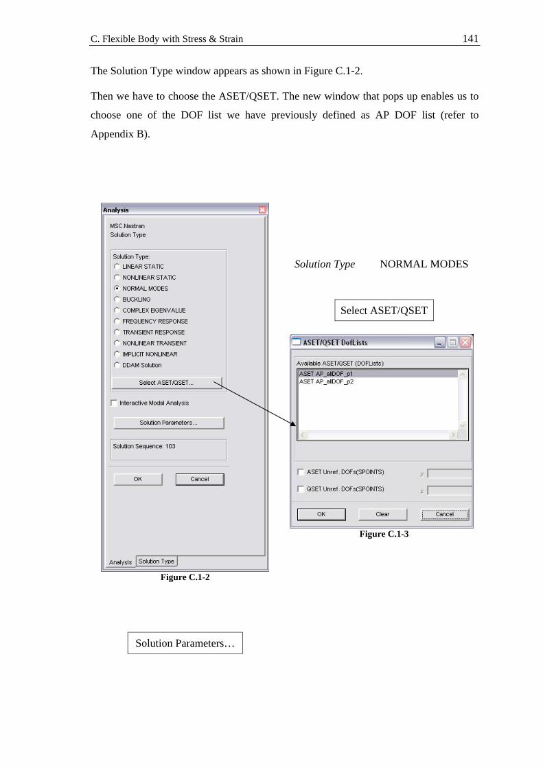
C. Flexible Body with Stress & Strain 141
The Solution Type window appears as shown in Figure C.1-2. Then we have to choose the ASET/QSET. The new window that pops up enables us to
choose one of the DOF list we have previously defined as AP DOF list (refer to
Appendix B).
Figure C.1-2
Solution Type NORMAL MODES
Select ASET/QSET
Figure C.1-3
Solution Parameters…
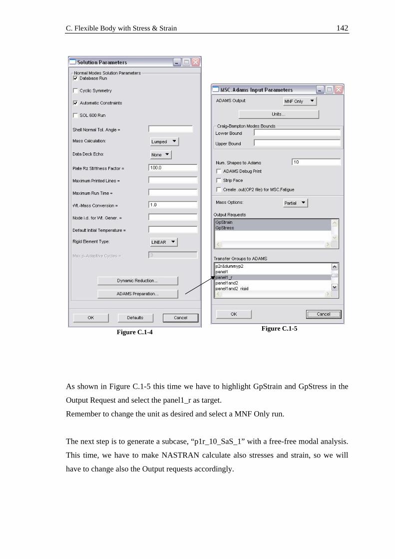
C. Flexible Body with Stress & Strain 142
Figure C.1-4
Figure C.1-5
As shown in Figure C.1-5 this time we have to highlight GpStrain and GpStress in the
Output Request and select the panel1_r as target.
Remember to change the unit as desired and select a MNF Only run.
The next step is to generate a subcase, “p1r_10_SaS_1” with a free-free modal analysis.
This time, we have to make NASTRAN calculate also stresses and strain, so we will
have to change also the Output requests accordingly.
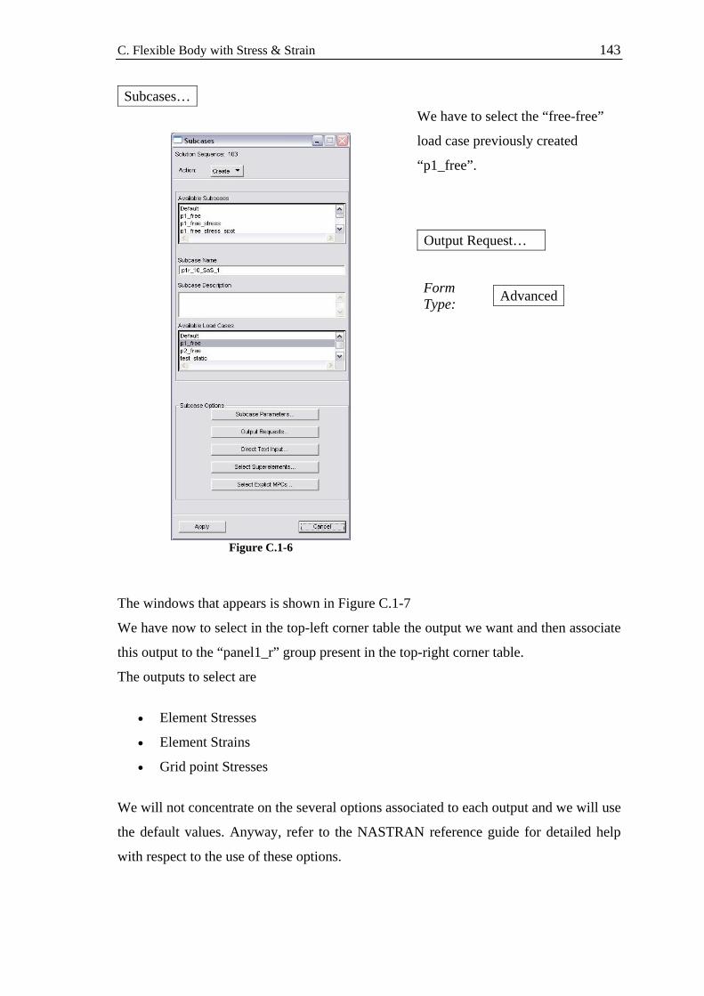
C. Flexible Body with Stress & Strain 143
Figure C.1-6
Subcases…
We have to select the “free-free”
load case previously created
“p1_free”.
Form Type: Advanced
Output Request…
The windows that appears is shown in Figure C.1-7
We have now to select in the top-left corner table the output we want and then associate
this output to the “panel1_r” group present in the top-right corner table.
The outputs to select are
• Element Stresses
• Element Strains
• Grid point Stresses
We will not concentrate on the several options associated to each output and we will use
the default values. Anyway, refer to the NASTRAN reference guide for detailed help
with respect to the use of these options.
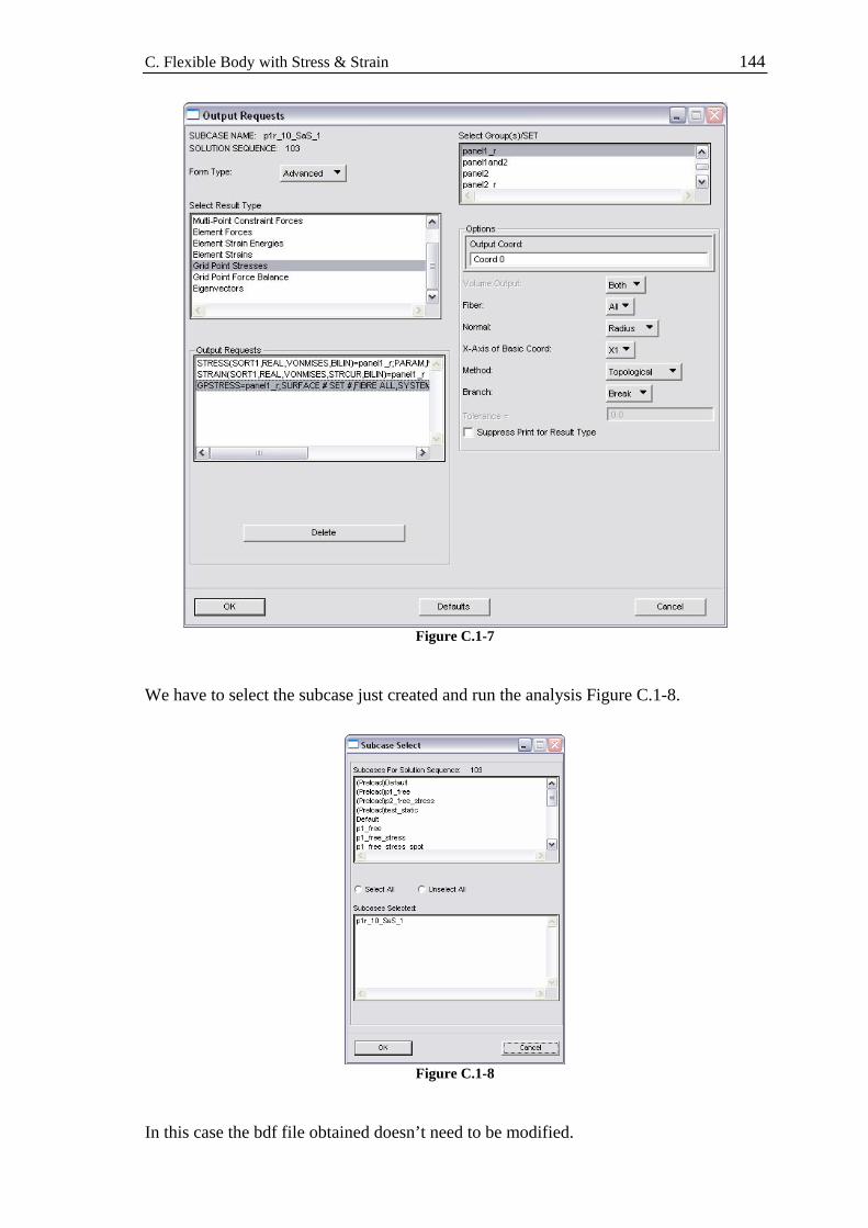
C. Flexible Body with Stress & Strain 144
Figure C.1-7
We have to select the subcase just created and run the analysis Figure C.1-8.
Figure C.1-8
In this case the bdf file obtained doesn’t need to be modified.

C. Flexible Body with Stress & Strain 145
C.2 Spot mesh S&S + PLOTEL
In this second approach we will add S&S information to the MNF file only in some
particular parts of the mesh. The reason for this choice is that usually we are not
interested in knowledge of the stress in the whole part, but only in particular highly
loaded zones.
For this reason we have to create a sub-group from panel1_r containing the mesh parts
on which we are interested in calculating the S&S.
panel1_r stress_p1
Figure C.2-1: Groups needed for generate a spot mesh stress model Then we need a PLOTEL grid (refer to Appendix B) to create the following groups
shown in Figure C.2-2 and Figure C.2-3
dummy_mesh_p1 stress_p1 stress_p1_dummy
Figure C.2-2: FEM groups for graphical and stress visualization in ADAMs
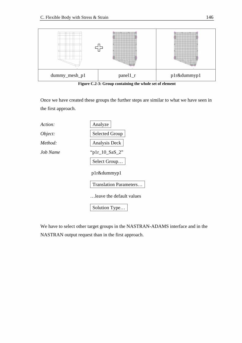
C. Flexible Body with Stress & Strain 146
dummy_mesh_p1 panel1_r p1r&dummyp1
Figure C.2-3: Group containing the whole set of element Once we have created these groups the further steps are similar to what we have seen in
the first approach.
Action: Analyze Object: Selected Group Method: Analysis Deck Job Name “p1r_10_SaS_2”
Select Group…
p1r&dummyp1
Translation Parameters…
…leave the default values
Solution Type… We have to select other target groups in the NASTRAN-ADAMS interface and in the
NASTRAN output request than in the first approach.

C. Flexible Body with Stress & Strain 147
Figure C.2-4
In the NASTRAN-ADAMS interface we
have to select stress_p1_dummy as
“Transfer Groups to ADAMS”
Then we have to create a new subcase associated with a free-free modal analysis “p1r_10_SaS_2” In the output request of this subcase we have to select the “stress_p1_dummy” as output
request:
• Element Stresses
• Element Strains
• Grid point Stresses
And associate each of them to the “stress_p1_dummy” group.
At this point we can run the analysis and obtain the MNF file.

C. Flexible Body with Stress & Strain 148
Figure C.2-5
After these changes we can run the Analysis Deck and obtain the bdf file.
In analogy of what we saw for the generation of a MNF file using the PLOTEL
elements grid the bdf file that we obtain needs to be manually modified.
Figure C.2-6 shows the changes to be applied to the bdf file. Actually the change that
has to be done is simply coping the OUTPUT(POST) command and his elements sets
and pasting them in front and changing the argument POST with PLOT.
In this way we impose the group “stress_p1_dummy” both for graphical purpose
(PLOT) and for S&S (POST) visualization in ADAMS

C. Flexible Body with Stress & Strain 149 $ NASTRAN input file created by the MSC MSC.Nastran input file $ translator ( MSC.Patran 13.1.116 ) on February 02, 2007 at 16:35:29. $ Direct Text Input for Nastran System Cell Section $ Direct Text Input for File Management Section $ Normal Modes Analysis, Database SOL 103 $ Direct Text Input for Executive Control CEND ….. $ Direct Text Input for this Subcase
PASTE HERE & change POST with PLOT
COPY
OUTPUT(POST) $ Elements for group : stress_p1_dummy SET 6 = 710024 THRU 710034,710037,710072 THRU 710083,710096 THRU 710159, 710196 THRU 710203,710472,710484 THRU 710490,710492 THRU 710499,710512, 710513 THRU 710531,710548 THRU 710622,710641 THRU 710669,710682, 710683 THRU 710716,710729,710730,710731,710732,710739 THRU 710766, 710777,710784,710785,710786,710789 THRU 710822,712763 THRU 712770, 712788 THRU 712803,712834 THRU 712849,712880 THRU 712896,712927, 712928 THRU 712944,712975 THRU 712983,713308 THRU 713321,713352, 713353 THRU 713374,713405 THRU 713416,713419 THRU 713426,713457, 713458 THRU 713465,713641 THRU 713646,713651 THRU 713656,713661, 713662 THRU 713688,713788 THRU 713798,713803 THRU 713812,713817, 713818 THRU 713826,713831 THRU 713839,714052 THRU 714081,714290, 714291 THRU 714319,714395 THRU 714408,714411,714412,714427 THRU 714470, 714545 THRU 714553,714555,714557,714558,714559,714560,714566,714568, 714577 THRU 714620,790111,790112,790121,790122,791211,791221,799443, 799444,799686 THRU 799697,799700,799701,799705 THRU 799710,799713, 799715,799718,799719,799720,799723,799725 THRU 799729,799733,799735, 799736 THRU 799742,799745,799747,799751 THRU 799755,799767 THRU 799771, 799775,799776,799777,799778,799782,799786 THRU 799794,799798,799802, 799803 THRU 799809,799813,799817 THRU 799824,799828,799832 THRU 799839, 799841,799842,799849 THRU 799855,799857,799861 THRU 799875,799877, 799878 THRU 799967,799968 SURFACE 1 SET 6,FIBRE ALL,SYSTEM CORD 0,AXIS X1,NORMAL R, TOPOLOGICAL ,BRANCH BREAK $ Elements for group : stress_p1_dummy SET 4 = 710024 THRU 710034,710037,710072 THRU 710083,710096 THRU 710159, 710196 THRU 710203,710472,710484 THRU 710490,710492 THRU 710499,710512, 710513 THRU 710531,710548 THRU 710622,710641 THRU 710669,710682, 710683 THRU 710716,710729,710730,710731,710732,710739 THRU 710766, 710777,710784,710785,710786,710789 THRU 710822,712763 THRU 712770, 712788 THRU 712803,712834 THRU 712849,712880 THRU 712896,712927, 712928 THRU 712944,712975 THRU 712983,713308 THRU 713321,713352, 713353 THRU 713374,713405 THRU 713416,713419 THRU 713426,713457, 713458 THRU 713465,713641 THRU 713646,713651 THRU 713656,713661, 713662 THRU 713688,713788 THRU 713798,713803 THRU 713812,713817, 713818 THRU 713826,713831 THRU 713839,714052 THRU 714081,714290, 714291 THRU 714319,714395 THRU 714408,714411,714412,714427 THRU 714470, 714545 THRU 714553,714555,714557,714558,714559,714560,714566,714568, 714577 THRU 714620,790111,790112,790121,790122,791211,791221,799443, 799444,799686 THRU 799697,799700,799701,799705 THRU 799710,799713, 799715,799718,799719,799720,799723,799725 THRU 799729,799733,799735, 799736 THRU 799742,799745,799747,799751 THRU 799755,799767 THRU 799771, 799775,799776,799777,799778,799782,799786 THRU 799794,799798,799802, 799803 THRU 799809,799813,799817 THRU 799824,799828,799832 THRU 799839, 799841,799842,799849 THRU 799855,799857,799861 THRU 799875,799877, 799878 THRU 799967,799968 BEGIN BULK …..
Result
$ NASTRAN input file created by the MSC MSC.Nastran input file $ translator ( MSC.Patran 13.1.116 ) on February 02, 2007 at 16:35:29. $ Direct Text Input for Nastran System Cell Section $ Direct Text Input for File Management Section $ Normal Modes Analysis, Database SOL 103 $ Direct Text Input for Executive Control CEND ….. $ Direct Text Input for this Subcase $$$$$$$$$$$$$$$$$$$$$$$$$$$$$$$$$$$$$$$$$$$$$$$$$$$$$$$$$$$$$$$$$$$$$$$ OUTPUT(PLOT) $ Elements for group : stress_p1_dummy SET 6 = 710024 THRU 710034,710037,710072 THRU 710083,710096 THRU 710159, 710196 THRU 710203,710472,710484 THRU 710490,710492 THRU 710499,710512, 710513 THRU 710531,710548 THRU 710622,710641 THRU 710669,710682, 710683 THRU 710716,710729,710730,710731,710732,710739 THRU 710766, 710777,710784,710785,710786,710789 THRU 710822,712763 THRU 712770, 712788 THRU 712803,712834 THRU 712849,712880 THRU 712896,712927, 712928 THRU 712944,712975 THRU 712983,713308 THRU 713321,713352, 713353 THRU 713374,713405 THRU 713416,713419 THRU 713426,713457, 713458 THRU 713465,713641 THRU 713646,713651 THRU 713656,713661, 713662 THRU 713688,713788 THRU 713798,713803 THRU 713812,713817, 713818 THRU 713826,713831 THRU 713839,714052 THRU 714081,714290, 714291 THRU 714319,714395 THRU 714408,714411,714412,714427 THRU 714470, 714545 THRU 714553,714555,714557,714558,714559,714560,714566,714568, 714577 THRU 714620,790111,790112,790121,790122,791211,791221,799443, 799444,799686 THRU 799697,799700,799701,799705 THRU 799710,799713, 799715,799718,799719,799720,799723,799725 THRU 799729,799733,799735, 799736 THRU 799742,799745,799747,799751 THRU 799755,799767 THRU 799771, 799775,799776,799777,799778,799782,799786 THRU 799794,799798,799802, 799803 THRU 799809,799813,799817 THRU 799824,799828,799832 THRU 799839, 799841,799842,799849 THRU 799855,799857,799861 THRU 799875,799877, 799878 THRU 799967,799968 SURFACE 1 SET 6,FIBRE ALL,SYSTEM CORD 0,AXIS X1,NORMAL R, TOPOLOGICAL ,BRANCH BREAK $ Elements for group : stress_p1_dummy SET 4 = 710024 THRU 710034,710037,710072 THRU 710083,710096 THRU 710159, 710196 THRU 710203,710472,710484 THRU 710490,710492 THRU 710499,710512, 710513 THRU 710531,710548 THRU 710622,710641 THRU 710669,710682, 710683 THRU 710716,710729,710730,710731,710732,710739 THRU 710766, 710777,710784,710785,710786,710789 THRU 710822,712763 THRU 712770, 712788 THRU 712803,712834 THRU 712849,712880 THRU 712896,712927, 712928 THRU 712944,712975 THRU 712983,713308 THRU 713321,713352, 713353 THRU 713374,713405 THRU 713416,713419 THRU 713426,713457, 713458 THRU 713465,713641 THRU 713646,713651 THRU 713656,713661, 713662 THRU 713688,713788 THRU 713798,713803 THRU 713812,713817, 713818 THRU 713826,713831 THRU 713839,714052 THRU 714081,714290, 714291 THRU 714319,714395 THRU 714408,714411,714412,714427 THRU 714470, 714545 THRU 714553,714555,714557,714558,714559,714560,714566,714568, 714577 THRU 714620,790111,790112,790121,790122,791211,791221,799443, 799444,799686 THRU 799697,799700,799701,799705 THRU 799710,799713, 799715,799718,799719,799720,799723,799725 THRU 799729,799733,799735, 799736 THRU 799742,799745,799747,799751 THRU 799755,799767 THRU 799771, 799775,799776,799777,799778,799782,799786 THRU 799794,799798,799802, 799803 THRU 799809,799813,799817 THRU 799824,799828,799832 THRU 799839, 799841,799842,799849 THRU 799855,799857,799861 THRU 799875,799877, 799878 THRU 799967,799968 $$$$$$$$$$$$$$$$$$$$$$$$$$$$$$$$$$$$$$$$$$$$$$$$$$$$$$$$$$$$$$$$$$$$$$$ OUTPUT(POST) $ Elements for group : stress_p1_dummy SET 6 = 710024 THRU 710034,710037,710072 THRU 710083,710096 THRU 710159, 710196 THRU 710203,710472,710484 THRU 710490,710492 THRU 710499,710512, 710513 THRU 710531,710548 THRU 710622,710641 THRU 710669,710682, 710683 THRU 710716,710729,710730,710731,710732,710739 THRU 710766, 710777,710784,710785,710786,710789 THRU 710822,712763 THRU 712770, 712788 THRU 712803,712834 THRU 712849,712880 THRU 712896,712927, 712928 THRU 712944,712975 THRU 712983,713308 THRU 713321,713352, 713353 THRU 713374,713405 THRU 713416,713419 THRU 713426,713457, 713458 THRU 713465,713641 THRU 713646,713651 THRU 713656,713661, 713662 THRU 713688,713788 THRU 713798,713803 THRU 713812,713817, 713818 THRU 713826,713831 THRU 713839,714052 THRU 714081,714290, 714291 THRU 714319,714395 THRU 714408,714411,714412,714427 THRU 714470, 714545 THRU 714553,714555,714557,714558,714559,714560,714566,714568, 714577 THRU 714620,790111,790112,790121,790122,791211,791221,799443, 799444,799686 THRU 799697,799700,799701,799705 THRU 799710,799713, 799715,799718,799719,799720,799723,799725 THRU 799729,799733,799735, 799736 THRU 799742,799745,799747,799751 THRU 799755,799767 THRU 799771, 799775,799776,799777,799778,799782,799786 THRU 799794,799798,799802, 799803 THRU 799809,799813,799817 THRU 799824,799828,799832 THRU 799839, 799841,799842,799849 THRU 799855,799857,799861 THRU 799875,799877, 799878 THRU 799967,799968 SURFACE 1 SET 6,FIBRE ALL,SYSTEM CORD 0,AXIS X1,NORMAL R, TOPOLOGICAL ,BRANCH BREAK $ Elements for group : stress_p1_dummy SET 4 = 710024 THRU 710034,710037,710072 THRU 710083,710096 THRU 710159, 710196 THRU 710203,710472,710484 THRU 710490,710492 THRU 710499,710512, 710513 THRU 710531,710548 THRU 710622,710641 THRU 710669,710682, 710683 THRU 710716,710729,710730,710731,710732,710739 THRU 710766, 710777,710784,710785,710786,710789 THRU 710822,712763 THRU 712770, 712788 THRU 712803,712834 THRU 712849,712880 THRU 712896,712927, 712928 THRU 712944,712975 THRU 712983,713308 THRU 713321,713352, 713353 THRU 713374,713405 THRU 713416,713419 THRU 713426,713457, 713458 THRU 713465,713641 THRU 713646,713651 THRU 713656,713661, 713662 THRU 713688,713788 THRU 713798,713803 THRU 713812,713817, 713818 THRU 713826,713831 THRU 713839,714052 THRU 714081,714290, 714291 THRU 714319,714395 THRU 714408,714411,714412,714427 THRU 714470, 714545 THRU 714553,714555,714557,714558,714559,714560,714566,714568, 714577 THRU 714620,790111,790112,790121,790122,791211,791221,799443, 799444,799686 THRU 799697,799700,799701,799705 THRU 799710,799713, 799715,799718,799719,799720,799723,799725 THRU 799729,799733,799735, 799736 THRU 799742,799745,799747,799751 THRU 799755,799767 THRU 799771, 799775,799776,799777,799778,799782,799786 THRU 799794,799798,799802, 799803 THRU 799809,799813,799817 THRU 799824,799828,799832 THRU 799839, 799841,799842,799849 THRU 799855,799857,799861 THRU 799875,799877, 799878 THRU 799967,799968 BEGIN BULK …..
Extracted from the original bdf file Modified bdf file (between $ the change) Figure C.2-6: Modification to apply to the BDF file
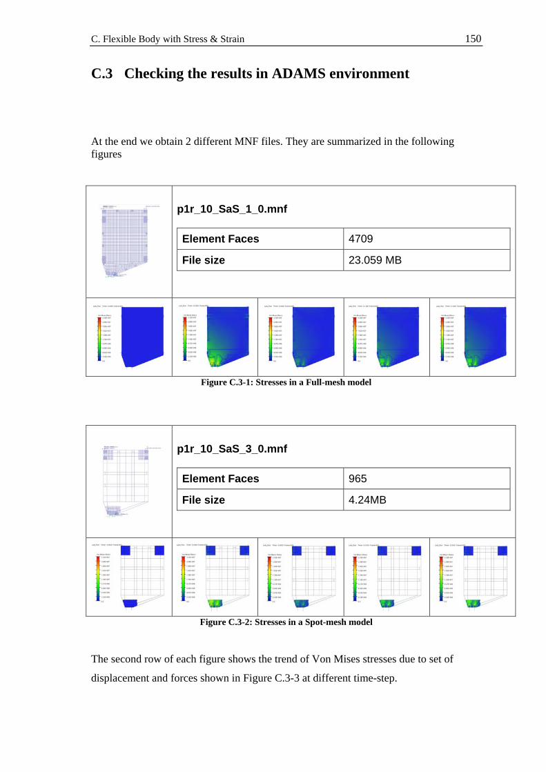
C. Flexible Body with Stress & Strain 150
C.3 Checking the results in ADAMS environment At the end we obtain 2 different MNF files. They are summarized in the following figures
p1r_10_SaS_1_0.mnf Element Faces 4709
File size 23.059 MB
Figure C.3-1: Stresses in a Full-mesh model
p1r_10_SaS_3_0.mnf Element Faces 965
File size 4.24MB
Figure C.3-2: Stresses in a Spot-mesh model The second row of each figure shows the trend of Von Mises stresses due to set of
displacement and forces shown in Figure C.3-3 at different time-step.

C. Flexible Body with Stress & Strain 151
Figure C.3-3: ADAMS model used to compare the stress with NASTRAN
As we can see from picture below the results obtained with the 2 different approaches
are the same.
Figure C.3-4: Comparison of stress between full mesh model and PLOTEL model
We can also compare the result of the ADAMS solution after the transient with a
NASTRAN static solution. The results we get are the following.
NASTRAN Von Mises Gp stress solution ADAMS Von Mises Gp stress solution Figure C.3-5: Comparison of stress between ADAMS and NASTRAN models
The results we obtained in ADAMS are the same of the NASTRAN static analysis.
Appendix D Flexible Bodies in ADAMS
The following tutorial will show how to import and set up a flexible body in the
ADAMS environment. We will show how to substitute a rigid body with its relative
flexible representation (MNF file) and how to use the main features of ADAMS/Flex.
D.1 Importing a flexible body
The model used in this tutorial is AMOS-3 on ground model. This choice is motivated
by the fact that the panels are subjected to the following three kinds of loads:
• Loads on Attachment Points (hinges forces and torques)
• Loads with an offset relative to the AP (CCL forces and torques and springs
forces)
• Loads on simple nodes (aerodynamic loads and torques)
We will show how to import the flexible representation of panel2. Figure D.1-1 shows
the model ready for the replacement of the rigid panel2. The forces are already split and
as remarked by the bottom left red square we have also added a new reference marker

D. Flexible Body in ADAMS 153
that, together with the two others markers located on the hinges, will help us to define
the right position and orientation of the flexible part.
Figure D.1-1: ADAMS starting rigid model
D.1.1 Alignment
Now we are ready to replace panel2 using the ADAMS pull down menu
Build → Flexible Bodies → Rigid to Flex…
The window shown in Figure D.1-3 appears. We have to fill the “Current Part” field
with the part that we want to replace and in the field below with the path to the related
MNF file. It is important here to notice that ADAMS does not include the MNF file into
the database but links it by following the path indicated. For this reason, to make the
model compatible also on other computers, it is better to delete all the backward part of
Loads on simple nodes
Loads on AP
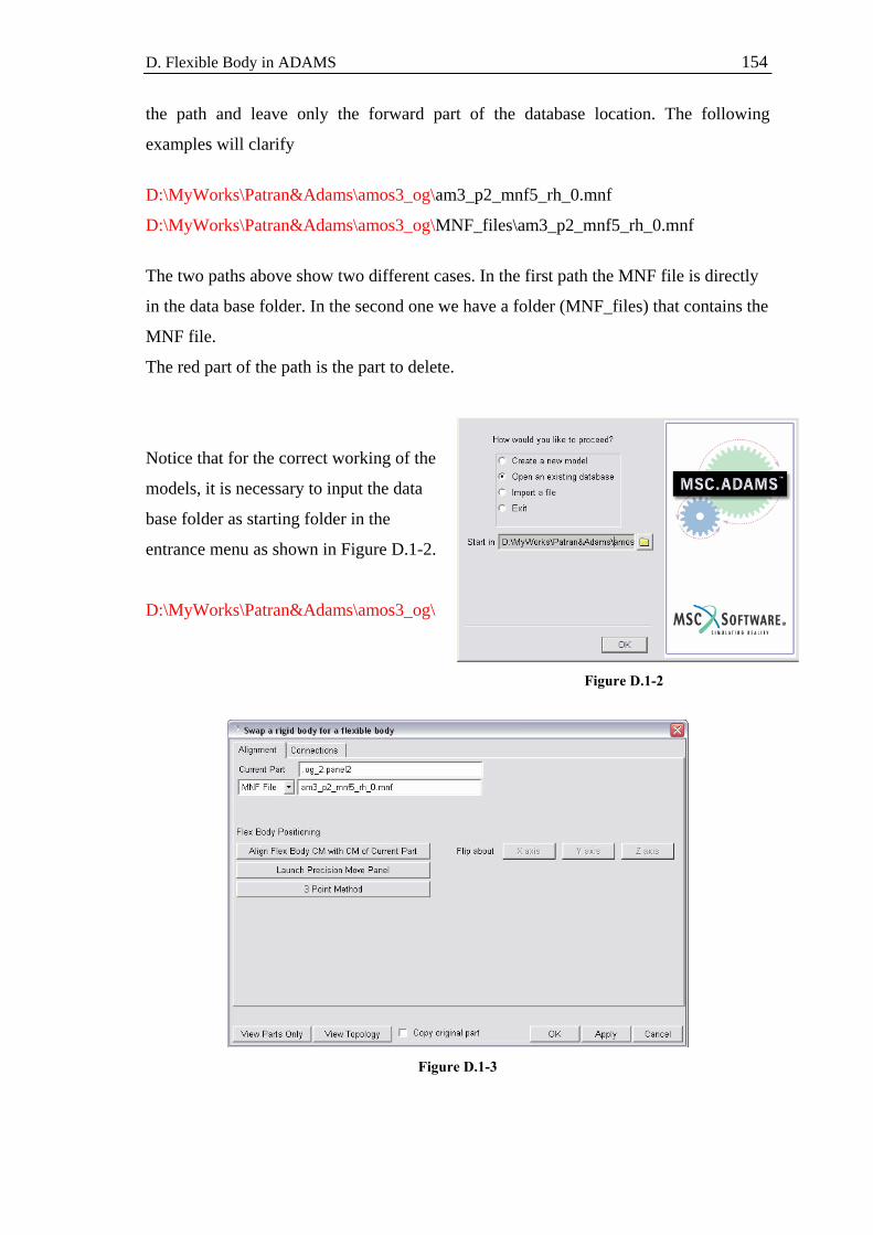
D. Flexible Body in ADAMS 154
the path and leave only the forward part of the database location. The following
examples will clarify
D:\MyWorks\Patran&Adams\amos3_og\am3_p2_mnf5_rh_0.mnf
D:\MyWorks\Patran&Adams\amos3_og\MNF_files\am3_p2_mnf5_rh_0.mnf
The two paths above show two different cases. In the first path the MNF file is directly
in the data base folder. In the second one we have a folder (MNF_files) that contains the
MNF file.
The red part of the path is the part to delete.
Notice that for the correct working of the
models, it is necessary to input the data
base folder as starting folder in the
entrance menu as shown in Figure D.1-2.
D:\MyWorks\Patran&Adams\amos3_og\
Figure D.1-2
Figure D.1-3
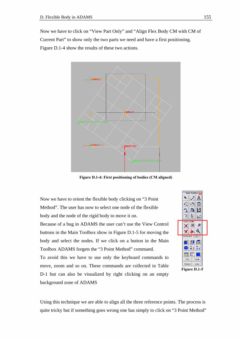
D. Flexible Body in ADAMS 155
Now we have to click on “View Part Only” and “Align Flex Body CM with CM of
Current Part” to show only the two parts we need and have a first positioning.
Figure D.1-4 show the results of these two actions.
Figure D.1-4: First positioning of bodies (CM aligned)
Now we have to orient the flexible body clicking on “3 Point
Method”. The user has now to select one node of the flexible
body and the node of the rigid body to move it on.
Because of a bug in ADAMS the user can’t use the View Control
buttons in the Main Toolbox show in Figure D.1-5 for moving the
body and select the nodes. If we click on a button in the Main
Toolbox ADAMS forgets the “3 Point Method” command.
To avoid this we have to use only the keyboard commands to
move, zoom and so on. These commands are collected in Table
D-1 but can also be visualized by right clicking on an empty
background zone of ADAMS
Figure D.1-5
Using this technique we are able to align all the three reference points. The process is
quite tricky but if something goes wrong one has simply to click on “3 Point Method”

D. Flexible Body in ADAMS 156
again and restart. When we select an AP of the flexible body and we are going to select
the hinge point on which to move it we have to pay attention to select the right reference
marker; that is because usually a lot of markers are present in the hinge surrounding
area and not all off them are exactly located in the hinge point.
To make the choice easier one can
zoom in on the hinge location and
click on the right mouse button
near the hinge central point. A
Select window pops up that help to
choose the right marker as shown
in Figure D.1-6
Figure D.1-6
Shift + f Front View
Shift + t Top View
Shift + r Right View
Shift + i Iso View
r Rotate XY
t Translate
z Zoom In/Out
w Zoom Box
f Fit to View Table D-1: Keyboard shortcuts to move the model
D.1.2 Connections
After the alignment of the three points the two parts should be superimposed as shown
in Figure D.1-7. Now we have to set up the connections between the two bodies; in
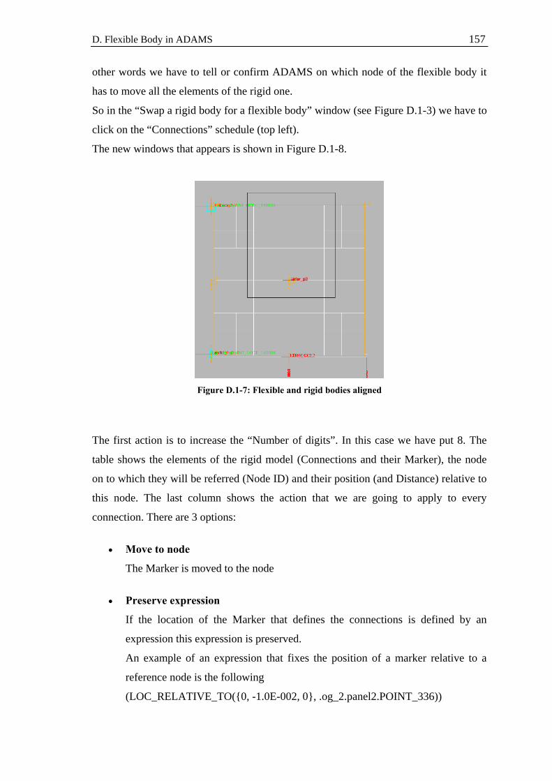
D. Flexible Body in ADAMS 157
other words we have to tell or confirm ADAMS on which node of the flexible body it
has to move all the elements of the rigid one.
So in the “Swap a rigid body for a flexible body” window (see Figure D.1-3) we have to
click on the “Connections” schedule (top left).
The new windows that appears is shown in Figure D.1-8.
Figure D.1-7: Flexible and rigid bodies aligned
The first action is to increase the “Number of digits”. In this case we have put 8. The
table shows the elements of the rigid model (Connections and their Marker), the node
on to which they will be referred (Node ID) and their position (and Distance) relative to
this node. The last column shows the action that we are going to apply to every
connection. There are 3 options:
• Move to node
The Marker is moved to the node
• Preserve expression
If the location of the Marker that defines the connections is defined by an
expression this expression is preserved.
An example of an expression that fixes the position of a marker relative to a
reference node is the following
(LOC_RELATIVE_TO({0, -1.0E-002, 0}, .og_2.panel2.POINT_336))
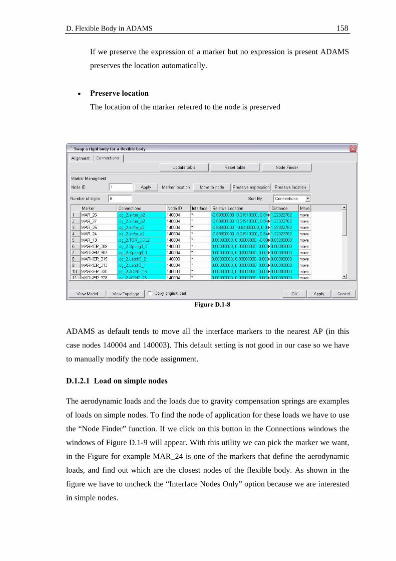
D. Flexible Body in ADAMS 158
If we preserve the expression of a marker but no expression is present ADAMS
preserves the location automatically.
• Preserve location
The location of the marker referred to the node is preserved
Figure D.1-8 ADAMS as default tends to move all the interface markers to the nearest AP (in this
case nodes 140004 and 140003). This default setting is not good in our case so we have
to manually modify the node assignment.
D.1.2.1 Load on simple nodes The aerodynamic loads and the loads due to gravity compensation springs are examples
of loads on simple nodes. To find the node of application for these loads we have to use
the “Node Finder” function. If we click on this button in the Connections windows the
windows of Figure D.1-9 will appear. With this utility we can pick the marker we want,
in the Figure for example MAR_24 is one of the markers that define the aerodynamic
loads, and find out which are the closest nodes of the flexible body. As shown in the
figure we have to uncheck the “Interface Nodes Only” option because we are interested
in simple nodes.
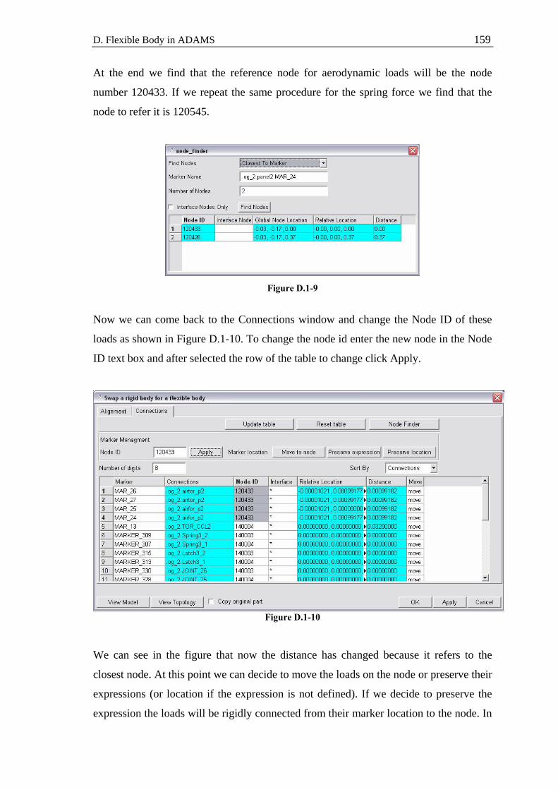
D. Flexible Body in ADAMS 159
At the end we find that the reference node for aerodynamic loads will be the node
number 120433. If we repeat the same procedure for the spring force we find that the
node to refer it is 120545.
Figure D.1-9
Now we can come back to the Connections window and change the Node ID of these
loads as shown in Figure D.1-10. To change the node id enter the new node in the Node
ID text box and after selected the row of the table to change click Apply.
Figure D.1-10
We can see in the figure that now the distance has changed because it refers to the
closest node. At this point we can decide to move the loads on the node or preserve their
expressions (or location if the expression is not defined). If we decide to preserve the
expression the loads will be rigidly connected from their marker location to the node. In

D. Flexible Body in ADAMS 160
this case anyway there is in no difference between the two cases because the distance is
already almost zero.
D.1.2.2 Loads with an offset respect to the AP The case comes up for the application of CCL loads. These loads are automatically
referred by ADAMS to the right AP (since is the closest one). What we have to do is
simply to preserve their expression because ADAMS will automatically connect them to
the AP with a rigid link as we want. Figure D.1-11 shows the table after the change. To
modify the action select the row and then click on “Preserve expression”.
Figure D.1-11
D.1.2.3 Loads on Attachment Points For what concern this loads we have simply to leave the table as it is. Locking at Figure
D.1-11 we can see in fact that the load markers that define loads on the AP are perfectly
coincident on the AP node (the distance is zero considering 8 digits).
If these markers are not perfectly aligned (error at the 4th or 5th digit), there was
something wrong in the previous orientation phase or that the dimensions of the rigid
panel do not match with the flexible ones. In both cases we can have some problems in
the model if we go on with the replacement.
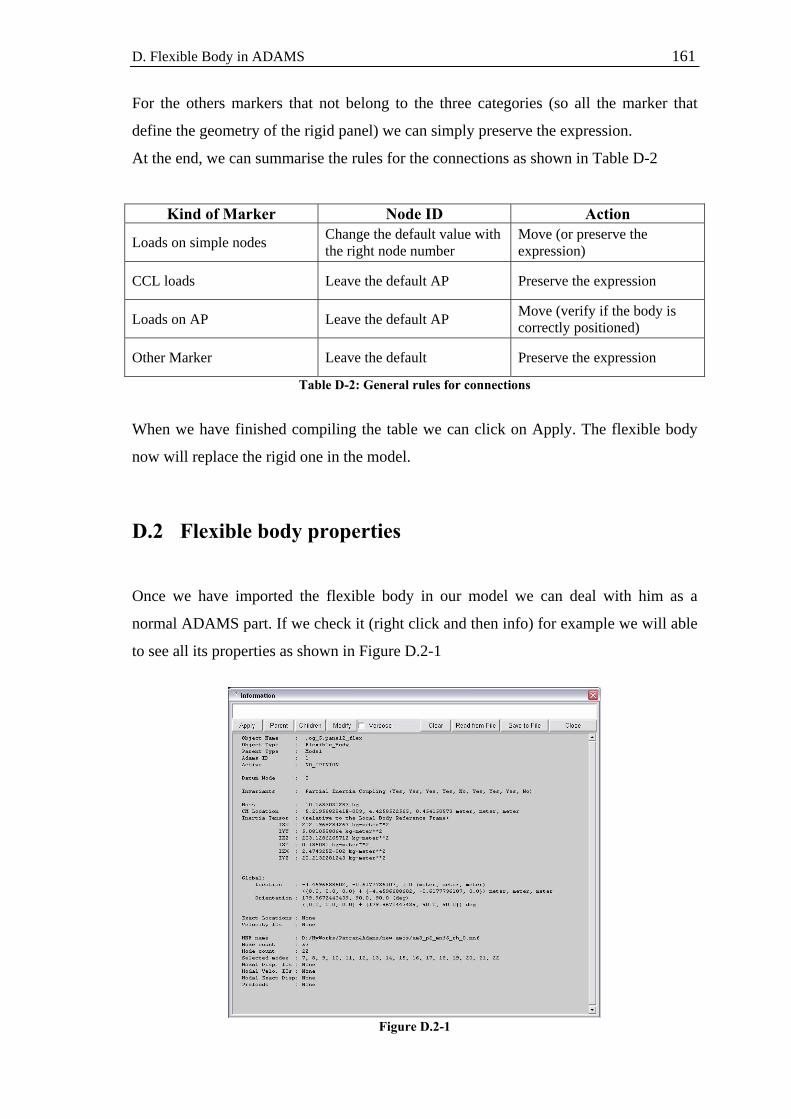
D. Flexible Body in ADAMS 161
For the others markers that not belong to the three categories (so all the marker that
define the geometry of the rigid panel) we can simply preserve the expression.
At the end, we can summarise the rules for the connections as shown in Table D-2
Kind of Marker Node ID Action
Loads on simple nodes Change the default value with the right node number
Move (or preserve the expression)
CCL loads Leave the default AP Preserve the expression
Loads on AP Leave the default AP Move (verify if the body is correctly positioned)
Other Marker Leave the default Preserve the expression
Table D-2: General rules for connections
When we have finished compiling the table we can click on Apply. The flexible body
now will replace the rigid one in the model.
D.2 Flexible body properties
Once we have imported the flexible body in our model we can deal with him as a
normal ADAMS part. If we check it (right click and then info) for example we will able
to see all its properties as shown in Figure D.2-1
Figure D.2-1

D. Flexible Body in ADAMS 162
To modify some of these properties (we can’t modify mass or inertia properties) one
can use the “Flexible Model Modify” panel (right click on the flexible body then
modify) shown in Figure D.2-2
Figure D.2-2
The main features of this interface are the Damping ratio control and the Modes control panel.
D.2.1 Damping ratio
If we do not specify modal damping when we create the flexible body, ADAMS/Flex
applies a default, non-zero critical damping ratio as follows:
• 1% damping for all modes with frequency lower than 100.
• 10% damping for modes with frequency in the 100 to 1000 range.
• 100% critical damping for modes with frequency above 1000.
We can change the default modal damping in three ways:
• Assign a single scalar critical damping ratio that ADAMS/Flex applies
uniformly to all modes.
Damping Ratio control Let the user to set up the damping of the model Initial Condition
Let the user to impose initial condition on position Velocity and modal displacement Modes Control Panel
Let the user to deactivate flexible modes of the body
Graphics Let the user to draw an outline (similar to the PLOTEL grid)
Inertia Modeling Let the user to set the mathematical flexible model to use
Deformation scale factor

D. Flexible Body in ADAMS 163
• Enter MSC.ADAMS run-time function expressions to create complex damping
phenomena in your flexible body. In addition, function expressions, such as
FXFREQ and FXMODE, allow us to apply different levels of damping to
individual modes.
• Control the damping using the DMPSUB user-written subroutine. DMPSUB lets
us set different levels of damping for different modes and the damping can vary
over time.
For more details on how to write custom damping function please refer to the ADAMS
help looking for DMPSUB, FXFREQ or FXMODE.
The generalized damping option enable the user to apply the same damping used in the
FEM model (if introduced in NASTRAN and included in the MNF file).
D.2.2 Modes Control With this interface the user can check all the modes that compose the Craig-Bampton
orthogonalized basis. The user can decide to deactivate the flexible modes or the range
of frequency that he considers useless.
Anyway, as we have seen in the theoretical background chapter, the high frequency
modes (eigenvectors) may be important for the representation of boundary modes in the
AP areas. From there, one should carefully check the changes generated in the model by
such deactivation.

Bibliography
[1] Ahmed A.Shabana. Dynamics of Multibody System, second edition. Cambridge
University Press
[2] E. Funaioli, A. Maggiore, U. Meneghetti. Lezioni di Meccanica Applicata alle
Macchine, vol II. Patron Editore
MSC Documentation
[3] ADAMS, NASTRAN & PATRAN reference guides
[4] ADAMS/Flex Theoretical Background
[5] NASTRAN/ADAMS interface documentation
[6] MSC online support (http://www.mscsoftware.com/support/)
EADS ASTRIUM Internal Documentation
[7] AMOS-3 Solar array – SG Deployment Analysis Report (AMSG-ASO-TN-2000-
0006)
[8] BEPI COLOMBO – Release and Deployment Analysis MPO S/A 2 (ARB4B-DNS-
AN-1000-0001)