1

Radu Serban and Edward J. HaugDepartment of Mechanical EngineeringThe University of IowaIowa City, Iowa 52242–1000, USA

ANALYTICAL DERIVATIVES

FOR MULTIBODY SYSTEM ANALYSES

ABSTRACT

Analytical formulas for kinematic and kinetic derivatives needed in multibody system analyses are derived. A broad

spectrum of problems, including implicit numerical integration, dynamic sensitivity analysis, and kinematic workspace

analysis, require evaluation of first derivatives of generalized inertia and force expressions and at least three derivatives of

algebraic constraint functions. In the setting of a formulation based on Cartesian generalized coordinates with Euler

parameters for orientation, basic identities are developed that enable practical and efficient computation of all derivatives

required for a large number of multibody mechanical system analyses. The formulation is verified through application to to a

spatial slider crank mechanism and a 14 body vehicle model. Efficiency of computation using the expressions derived is

compared with results obtained employing finite differences, showing significant computational advantage using the

analytically derived expressions.

1 INTRODUCTION

Three different areas of multibody system analysis are considered. The common requirement for numerical methods used

in these types of analysis is the availability of higher order derivatives of both the differential equations of motion and of the

algebraic constraint equations. The three types of analysis under consideration are as follows:

(1) numerical implicit integration of the differential–algebraic equations (DAE) of motion for simulation of stiff

mechanical systems;

(2) dynamic sensitivity analysis for design optimization, parameter estimation, and model correlation;

(3) kinematic workspace analysis of mechanisms.

Next, each of these problems is shortly described and required derivatives for numerical solution are identified.

2

1.1 Kinematic and Dynamic Analysis

Two forms of equations that characterize the dynamics of a multibody system may be generated, (1) the state–space

representation and (2) the descriptor form. The minimal dimension state–space ordinary differential equation (ODE) form of

the equations of motion occurs when the multibody system is tree–configured and relative coordinates are used. The presence

of kinematic closed–loops results in a DAE form of the equations of motion, called the descriptor form. The focus here is on

the descriptor form, using Cartesian generalized coordinates (Haug, 1989).

For a system described by n generalized coordinates q and m constraint equations, the equations of motion can be written

in the descriptor form

M^

q..��

^ T

q� � Q^ (1)

associated with the algebraic constraint equations

�^

(q, t) � 0 (2)

where q, q. , and q.. are n� 1 vectors representing generalized positions, velocities, and accelerations; M

^(q) is the n� n

symmetric generalized inertia, or mass matrix; Q^

(q, q., t) is the n� 1 generalized force vector; � is the m� 1 vector of

Lagrange multipliers; and �^ q(q, t) � ���^ i(q, t)�qj� is the m� n constraint Jacobian matrix. It is assumed in this derivation that

the kinematic constraint Jacobian matrix has full row rank. Equations 1 and 2 thus represent an index–3 DAE (Brenan et al.,

1989).

The position constraints of Eq. 2 can be differentiated with respect to time to yield the kinematic velocity and acceleration

constraint equations,

�^

qq.��

^t � 0 (3)

�^

qq..� ��^ qq

. �qq.� 2�

^tqq

.��

^tt � 0 (4)

where subscript t denotes partial derivative with respect to time.

There are many methods for integrating the DAE of Eqs. 1 through 4. Discussions of such methods are presented by

Brenan et al. (1989), Hairer and Wanner (1996), and Potra (1994). Numerically stiff systems, which often arise due to

bushings and stiff compliant elements, require the use of implicit integration methods. Only these implicit methods exhibit the

required stability to deal with such systems (Haug et al., 1997a, 1997b). Regardless of which implicit integrator is used,

3

derivatives of all terms in Eqs. 1 through 4 with respect to both generalized coordinates and velocities are required. The

derivatives to be evaluated are as follows: �M^q..�

q, ��^ T

q��q

, Q^

q, Q^

q. , ��^ qq

. �q, ��^ qq

..�q, ���^ qq

. �qq. �

q

, ���^ qq. �

qq. �

q.

.

1.2 Dynamic Sensitivity Analysis

Numerous problems in multibody mechanical system analysis can be formulated as optimization problems with respect

to dynamic behavior of the system. A nonlinear programming problem must then be solved. Optimization algorithms are most

efficient if accurate derivative information is provided. Dynamic design sensitivity analysis of multibody systems thus

represents the link between optimization tools and modelling and simulation tools.

Two methods are commonly used to generate sensitivity information. The most straightforward approach is the direct

differentiation method, which differentiates the differential–algebraic equations of motion with respect to parameters

(Krishnaswami et. al., 1983; Chang and Nikravesh, 1985; Haug, 1987). The second method is the adjoint variable method, in

which sensitivities are obtained as solutions of differential–algebraic equations that are adjoint to the equations of motion. The

adjoint variable method has been extensively applied in both optimal control and optimal design (Haug and Ehle, 1982; Haug,

1987; Bestle and Eberhard, 1992; Bestle and Seybold, 1992). Both methods require derivatives of terms in the DAE of motion

with respect to parameters. Use of the chain rule of differentiation in both methods reduces this problem to finding derivatives

of these terms with respect to generalized states and velocities. Therefore, all derivatives noted above for implicit integration

of the equations of motion are needed to generate the sensitivity equations.

1.3 Workspace analysis

The problem of defining achievable sets in the output space of a mechanism is known as kinematic workspace analysis.

Domains of operation (accessible output, operational envelope), domains of interference, and domains of mobility can be

treated in a unified fashion (Haug et al., 1996). Most research has focused on describing mechanism workspaces by defining

their boundaries. Analytical conditions for workspace boundaries in special mechanisms have been used by a number of

authors (Tsai and Soni, 1981; Yang and Lee, 1983; Freudstein and Primerose, 1984). For general mechanisms, Litvin (1980)

used the implicit function theorem to obtain criteria for workspaces, relating them to singular configurations of mechanisms.

Analytical criteria and numerical methods for mapping boundaries of workspaces, using Jacobian matrix row rank deficiency

conditions, have been developed by Jo and Haug (1989), Wang and Wu (1993), Haug et al. (1996), and Adkins (1996). The

4

following quantities related to the kinematics of the underlying mechanism must be evaluated: ��^ T

q��q

, ���^ T

q��q

���

,

���^ T

q��q

��q

, ��^ q��q, where �, �, and � are vectors of appropriate dimension.

1.4 Choice of Generalized Coordinates

A common point of departure for many of the intended capabilities of a general multibody analysis tool is the ability to

obtain derivatives of both the differential equations of motion and the algebraic constraint equations. In modelling a multibody

system, the first important choice to be made is that of generalized coordinates to describe its position and motion. The

Cartesian coordinate formulation with Euler parameters for orientation is particularly attractive, from the point of view of

systematic analysis, because of the simple structure of the resulting equations. The form of the orientation matrix in terms of

Euler parameters yields bilinear forms in the Euler parameter vector p for constraint derivatives. Theoretically, this implies

that as many derivatives as desired can be taken. Advantages of Cartesian coordinates can be summarized as follows: (1) the

formulation yields simple forms of the coefficient matrices in the equations of motion, so constraint equations can be

generated in a consistent way; (2) the matrices involved are sparse; (3) position, velocity, and acceleration information for each

body is directly obtained; and (4) the constraints are established at a local level, in the sense that constraint equations for a

given joint involve only the coordinates of the two bodies that are connected by the joint. Therefore, the constraint equations

are independent of the complexity of the system.

1.5 Equations of Motion of Multibody Dynamics with Cartesian Coordinates

In Cartesian coordinates with Euler parameters for orientation, the equations of motion of Eqs. 1 and 2 are (Haug, 1989)

�M0 04GTJ�G��r

..

p..�� ��T

r

�Tp

0�

PTp�� � � FA

2GTn�A � 8G. T

J�G.p� (5)

�(r , p, t) � 0 (6)

�P(p) � 0 (7)

where M � diag{ miI 3} is a block–diagonal matrix containing the masses of the nb bodies, J� � diag{ J� i} is the block–diagonal

inertia matrix of the system, r � { r i} is the vector of body positions, p � { pi} is the vector of Euler parameters, FA is the vector

of applied forces, n�A is the vector of applied torques, G is a 3�4 matrix defined as G(p) � [� e,� e~ � e0I ] , and �P is the

vector of Euler parameter normalization constraints. Here, e~ is the 3�3 skew–symmetric matrix defined by

5

e~ ���

0e3

� e2

� e3

0e1

e2

� e1

0 �

(8)

As shown in this paper, a relatively small number of basic identities enables computation of all required derivatives of both

kinematic and kinetic terms arising in each of the analyses discussed above. Explicit forms for derivatives of basic quantities

are obtained. Therefore, this approach is expected to be more efficient than using automatic differentiation methods (Bischof et

al., 1996). When evaluating higher order derivatives, automatic differentiation codes differentiate a lower order derivative and

thus cannot take advantage of simplifying identities that may exist, such as Euler parameter normalization constraints.

2 BASIC IDENTITIES

Derivatives of expressions used as basic building blocks in generating required kinematic and kinetic derivatives are

obtained in this section. The identities derived are subsequently applied to obtain higher order derivatives of the constraint

equations and of common force elements. When using Cartesian coordinates with Euler parameters to model a multibody

system, the generalized inertia matrix has a simple block–diagonal form. Obtaining derivatives of terms involving this matrix

is therefore straightforward.

In the Cartesian coordinate formulation, dependencies on states, velocities, and parameters that appear in the coefficients

of the DAE of motion are well defined. The most complicated terms are those involving the Jacobian of the constraint

equations. Derivatives with respect to Euler parameters are the principal focus, since dependency on position vectors is

straightforward.

A quantity that arises in many terms of interest is representation of a body–fixed vector relative to the global reference

frame. Let a be a constant body–fixed vector, represented in the body reference frame, and let p � �e0; eT�T be the vector of

Euler parameters that defines the orientation of the body reference frame relative to a global reference frame. Then, the

orientation transformation matrix is (Haug, 1989)

A(p) � (2e20 � 1)I � 2(eeT � e0e

~) (9)

and the global representation of the body–fixed vector a is

a � A(p)a � (2e20 � 1)a � 2(eeTa � e0e

~a) (10)

The derivative of this quantity with respect to the vector of Euler parameters is given by the following sequence of operations:

��e0

(A(p)a) � 4e0a � 2a~

e (11)

��e

(A(p)a) � 2�eTaI � eaT � e0a~ � � 2�aeT � eaT � (e0I � e~)a

~ � (12)

6

��p

(A(p)a�) � � ��e0

(A(p)a�) ; ��e

(A(p)a�)� � 2�a�pT � �(e0I � e~)a�; ea�T � (e0I � e~)a�~ � (13)

A 3�4 matrix B^(p, a�) is defined as

B^(p, a�) � �(e0I � e~)a; ea�T � (e0I � e~)a�

~ � (14)

and the related 3�4 matrix B(p, a�) is defined as

B(p, a�) � 2�a�pT � B^(p, a�) (15)

Therefore, the derivative in Eq. 13 can be simply expressed as

��p

(A(p)a�) � B(p, a�) (16)

Note that the 3�3 orientation transformation matrix A(p) involves quadratic terms in p, so it is expected that linear

expressions in p will occur after differentiation with respect to p in Eq. 13. Indeed, the matrices B^ and B are linear in the Euler

parameters. Moreover, these matrices have a commutativity property involving two 4–dimensional vectors, pi and pj, namely,

B^(pi, a�)pj � (e0iI � e~ i)a�e0j � eia�Tej � (e0iI � e~ i)a�

~ej

� (e0jI � e~ j)a�e0i � e0ja�~

ei � eieTj a� � e~ ie

~ja�

� (e0jI � e~ j)a�e0i � eja�Tei � (e0jI � e~ j)a�~

ei � B^(pj, a�)pi

(17)

and

B(pi, a�)pj � 2�a�pTi pj � B

^(pi, a�)pj � 2�a�pT

j pi � B^(pj, a�)pi � B(pj, a�)pi (18)

As a direct consequence of these commutativity properties, the following result is obtained:

��pi

B(pi, a�)pj� � �

�pi

B(pj, a�)pi� � B(pj, a�) (19)

Calculation of the derivative of BT(p, a�)� with respect to p is also required. Note, from Eq. 14, that

B^ T

(p, a�)� � � a�T(e0I � e~)�

a�eT�� a�

~(e0I � e~)�

� (20)

The derivative of this expression with respect to the Euler parameter e0 is

��e0B^ T

(p, a�)�� � �a�T�

a�~�� (21)

7

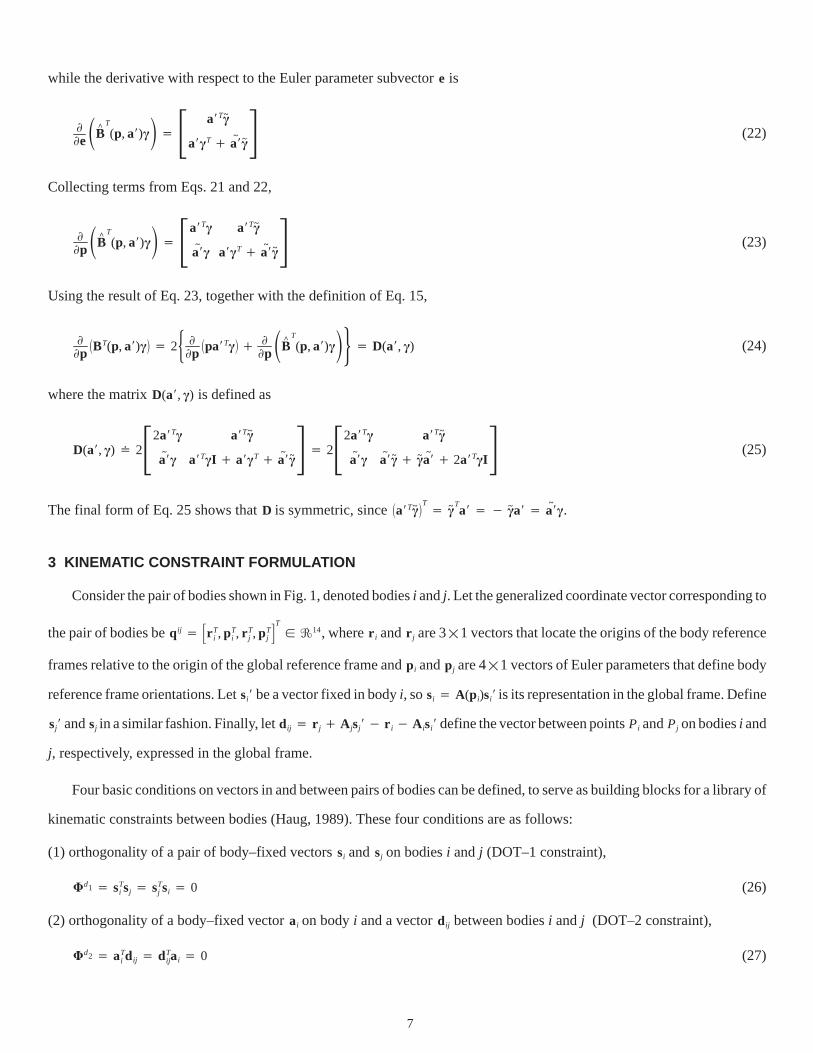
while the derivative with respect to the Euler parameter subvector e is

��e�B^ T

(p, a )�� � � a T�~

a �T � a ~�~� (22)

Collecting terms from Eqs. 21 and 22,

��p�B^ T

(p, a )�� � �a T�

a ~�

a T�~

a �T � a ~�~� (23)

Using the result of Eq. 23, together with the definition of Eq. 15,

��p

�BT(p, a )�� � 2 ��p�pa T

�� � ��p�B^ T

(p, a )�� � D(a , �) (24)

where the matrix D(a , �) is defined as

D(a , �) � 2�2a T�

a ~�

a T�~

a T�I � a �T � a

~�~� � 2�2a T

�

a ~�

a T�~

a ~�~ � �

~a ~� 2a T

�I� (25)

The final form of Eq. 25 shows that D is symmetric, since �a T�~�T � �

~Ta � � �

~a � a ~�.

3 KINEMATIC CONSTRAINT FORMULATION

Consider the pair of bodies shown in Fig. 1, denoted bodies i and j. Let the generalized coordinate vector corresponding to

the pair of bodies be qij � �r Ti , pT

i , r Tj , pT

j�T � �

14, where r i and r j are 3�1 vectors that locate the origins of the body reference

frames relative to the origin of the global reference frame and pi and pj are 4�1 vectors of Euler parameters that define body

reference frame orientations. Let si be a vector fixed in body i, so si � A(pi)si is its representation in the global frame. Define

sj and sj in a similar fashion. Finally, let dij � r j � A jsj � r i � A isi define the vector between points Pi and Pj on bodies i and

j, respectively, expressed in the global frame.

Four basic conditions on vectors in and between pairs of bodies can be defined, to serve as building blocks for a library of

kinematic constraints between bodies (Haug, 1989). These four conditions are as follows:

(1) orthogonality of a pair of body–fixed vectors si and sj on bodies i and j (DOT–1 constraint),

�d1 � sT

i sj � sTj si � 0 (26)

(2) orthogonality of a body–fixed vector ai on body i and a vector dij between bodies i and j (DOT–2 constraint),

�d2 � aT

i dij � dTijai � 0 (27)

8

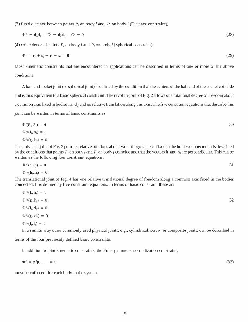
(3) fixed distance between points Pi on body i and Pj on body j (Distance constraint),

�ss� dT

ijdij � C2 � dTjidji � C2 � 0 (28)

(4) coincidence of points Pi on body i and Pj on body j (Spherical constraint),

�s � r j � sj � r i � si � 0 (29)

Most kinematic constraints that are encountered in applications can be described in terms of one or more of the above

conditions.

A ball and socket joint (or spherical joint) is defined by the condition that the centers of the ball and of the socket coincide

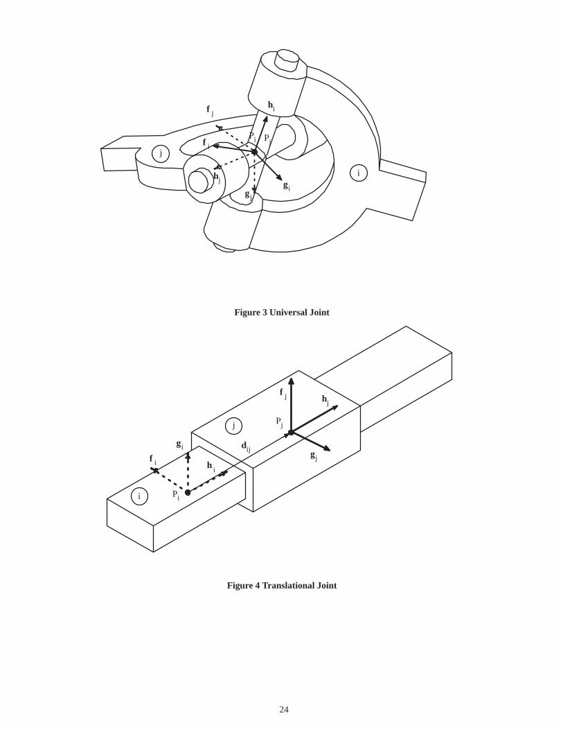
and is thus equivalent to a basic spherical constraint. The revolute joint of Fig. 2 allows one rotational degree of freedom about

a common axis fixed in bodies i and j and no relative translation along this axis. The five constraint equations that describe this

joint can be written in terms of basic constraints as

�s(Pi, Pj) � 0

�d1(f i, hj) � 0

�d1(gi, hj) � 0

30

The universal joint of Fig. 3 permits relative rotations about two orthogonal axes fixed in the bodies connected. It is describedby the conditions that points Pi on body i and Pj on body j coincide and that the vectors hi and hj are perpendicular. This can bewritten as the following four constraint equations:

�s(Pi, Pj) � 0

�d1(hi, hj) � 0

31

The translational joint of Fig. 4 has one relative translational degree of freedom along a common axis fixed in the bodiesconnected. It is defined by five constraint equations. In terms of basic constraint these are

�d1(gi, hj) � 0

�d1(f i, f j) � 0

�d1(f i, hj) � 0

�d2(gi, dij) � 0

�d2(f i, dij) � 0

32

In a similar way other commonly used physical joints, e.g., cylindrical, screw, or composite joints, can be described in

terms of the four previously defined basic constraints.

In addition to joint kinematic constraints, the Euler parameter normalization constraint,

�Pi � pT

i pi � 1 � 0 (33)

must be enforced for each body in the system.

9

4 DERIVATIVES OF KINEMATIC CONSTRAINT EXPRESSIONS

With the formulas derived in Section 2, basic constraint equations and their derivatives can be evaluated. A detailed

derivation of derivatives for the spherical constraint is presented here. Derivatives of the other three basic constraints, using the

same approach, are presented in Appendix A.

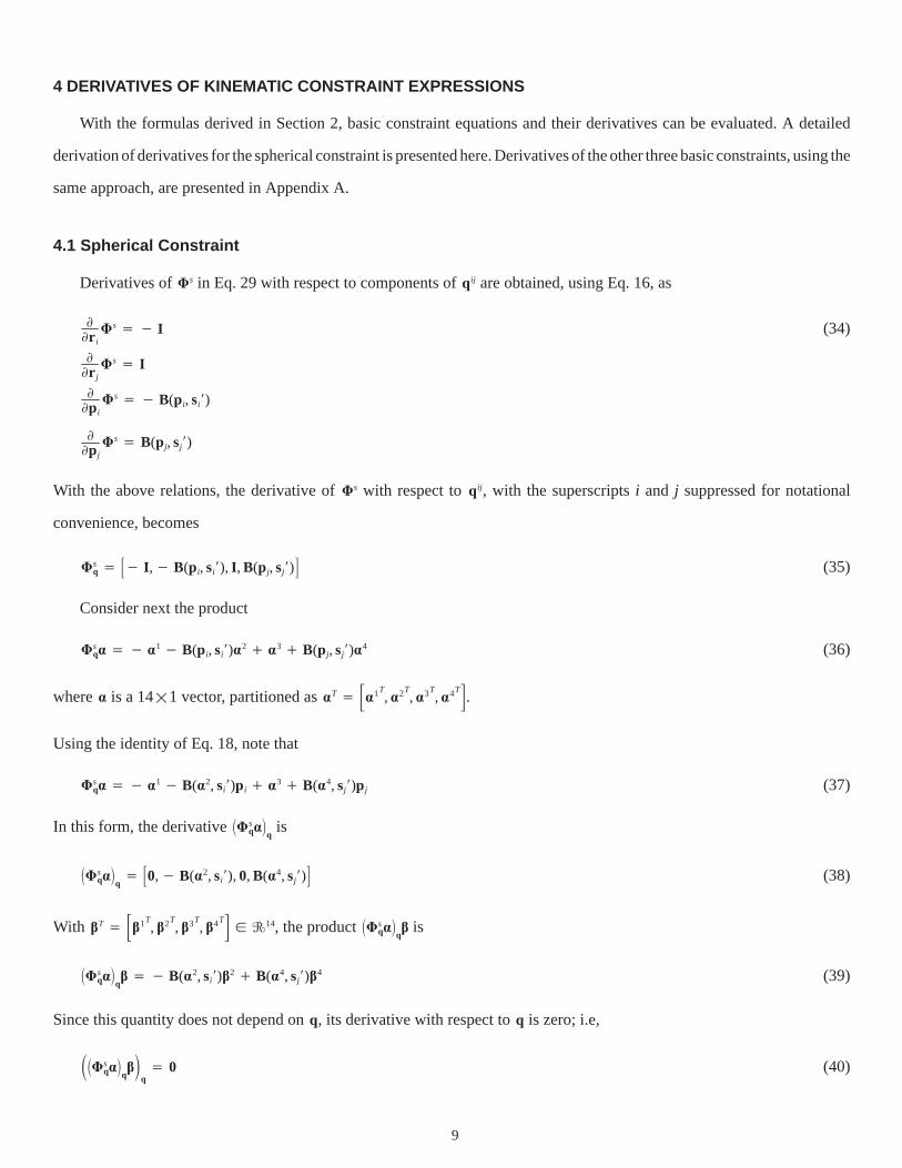
4.1 Spherical Constraint

Derivatives of �s in Eq. 29 with respect to components of qij are obtained, using Eq. 16, as

��r i

�s � � I

��r j

�s � I

��pi

�s � � B(pi, si)

��pj

�s � B(pj, sj)

(34)

With the above relations, the derivative of �s with respect to qij , with the superscripts i and j suppressed for notational

convenience, becomes

�sq � �� I ,� B(pi, si), I , B(pj, sj)� (35)

Consider next the product

�sq� � � �

1 � B(pi, si)�2 � �3 � B(pj, sj)�4 (36)

where � is a 14�1 vector, partitioned as �T � ��1T,�2T

,�3T,�4T�.

Using the identity of Eq. 18, note that

�sq� � � �

1 � B(�2, si)pi � �3 � B(�4, sj)pj (37)

In this form, the derivative ��sq�q is

��sq�q � �0,� B(�2, si), 0, B(�4, sj)� (38)

With �T � ��1T, �2T

, �3T, �4T� � �

14, the product ��sq�q� is

��sq�q� � � B(�2, si)�2 � B(�4, sj)�4 (39)

Since this quantity does not depend on q, its derivative with respect to q is zero; i.e,

���sq�q�q

� 0 (40)

10

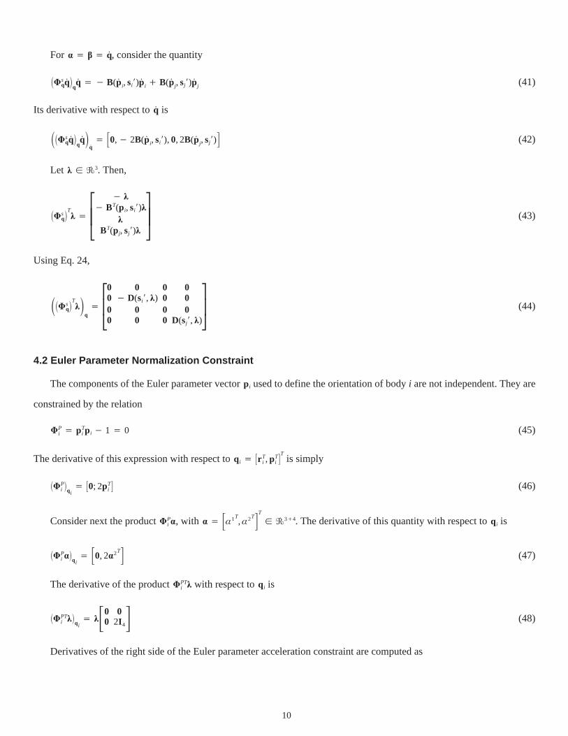
For � � � � q. , consider the quantity

��sqq

. �qq.� � B(p

.i, si)p

.i � B(p

.j, sj)p

.j (41)

Its derivative with respect to q. is

���sqq

. �qq. �

q.� �0,� 2B(p

.i, si), 0, 2B(p

.j, sj)� (42)

Let � � �3. Then,

��sq�

T� ��

�

� �

� BT(pi, si)��

BT(pj, sj)�

�(43)

Using Eq. 24,

���sq�

T��

q��

�

0000

0� D(si, �)

00

0000

000

D(sj, �)

�(44)

4.2 Euler Parameter Normalization Constraint

The components of the Euler parameter vector pi used to define the orientation of body i are not independent. They are

constrained by the relation

�Pi � pT

i pi � 1 � 0 (45)

The derivative of this expression with respect to qi � �r Ti , pT

i�T is simply

��Pi�qi� �0; 2pT

i� (46)

Consider next the product �Pi �, with � � ��1T

,�2T�T

� �3�4. The derivative of this quantity with respect to qi is

��Pi ��qi� �0, 2�2T� (47)

The derivative of the product �PTi � with respect to qi is

��PTi ��

qi� ��00 0

2I 4� (48)

Derivatives of the right side of the Euler parameter acceleration constraint are computed as

11

����Pi�qiq.

i�

qi

q.

i�qi

� 0 (49)

and

����Pi�qiq.

i�

qi

q.

i�q.

i

� �0, 4p. T

i� 50

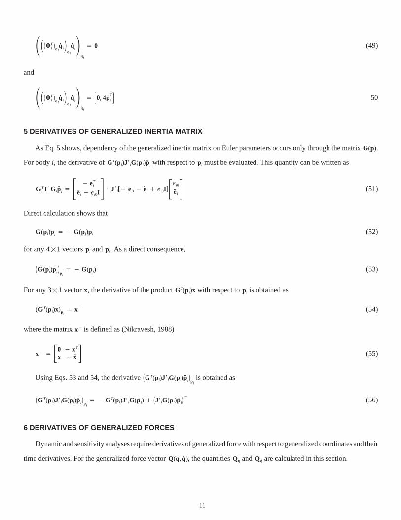
5 DERIVATIVES OF GENERALIZED INERTIA MATRIX

As Eq. 5 shows, dependency of the generalized inertia matrix on Euler parameters occurs only through the matrix G(p).

For body i, the derivative of GT(pi)J iG(pi)p..

i with respect to pi must be evaluated. This quantity can be written as

GTi J iG ip

..i � � � eT

i

e~ i � ei0I� � J i[� ei,� e~ i � ei0I ]�e

..i0

e..

i� (51)

Direct calculation shows that

G(pi)pj � � G(pj)pi (52)

for any 4�1 vectors pi and pj. As a direct consequence,

�G(pi)pj�

pi� � G(pj) (53)

For any 3�1 vector x, the derivative of the product GT(pi)x with respect to pi is obtained as

(GT(pi)x)pi� x� (54)

where the matrix x� is defined as (Nikravesh, 1988)

x� � �0x � xT

� x~ � (55)

Using Eqs. 53 and 54, the derivative �GT(pi)J iG(pi)p..

i�pi is obtained as

�GT(pi)J iG(pi)p..

i�pi� � GT(pi)J iG(p

..i) � �J iG(pi)p

..i�� (56)

6 DERIVATIVES OF GENERALIZED FORCES

Dynamic and sensitivity analyses require derivatives of generalized force with respect to generalized coordinates and their

time derivatives. For the generalized force vector Q(q, q.), the quantities Qq and Qq

. are calculated in this section.

12

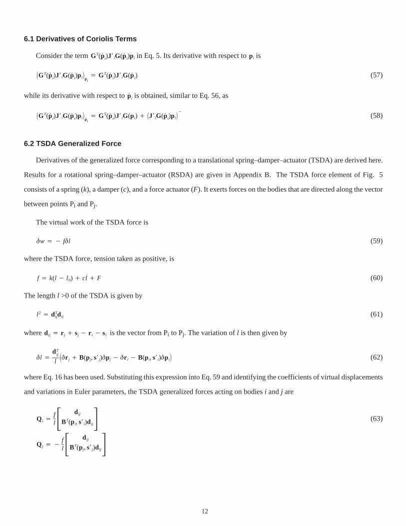
6.1 Derivatives of Coriolis Terms

Consider the term GT(p.

i)J� iG(p.

i)pi in Eq. 5. Its derivative with respect to pi is

�GT(p.

i)J� iG(p.

i)pi�pi� GT(p

.i)J� iG(p

.i) (57)

while its derivative with respect to p.

i is obtained, similar to Eq. 56, as

�GT(p.

i)J� iG(p.

i)pi�p.

i� GT(p

.i)J� iG(pi) � �J� iG(p

.i)pi

�� (58)

6.2 TSDA Generalized Force

Derivatives of the generalized force corresponding to a translational spring–damper–actuator (TSDA) are derived here.

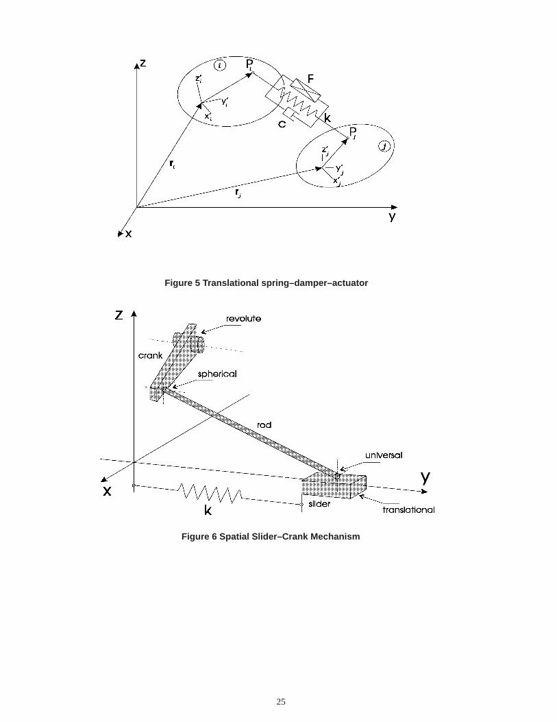
Results for a rotational spring–damper–actuator (RSDA) are given in Appendix B. The TSDA force element of Fig. 5

consists of a spring (k), a damper (c), and a force actuator (F). It exerts forces on the bodies that are directed along the vector

between points Pi and Pj.

The virtual work of the TSDA force is

�w � � f�l (59)

where the TSDA force, tension taken as positive, is

f � k(l � l 0) � cl.� F (60)

The length l >0 of the TSDA is given by

l 2 � dTijdij (61)

where dij � r j � sj � r i � si is the vector from Pi to Pj. The variation of l is then given by

�l �dT

ij

l��r j � B(pj, s� j)�pj � �r i � B(pi, s� i)�pi

� (62)

where Eq. 16 has been used. Substituting this expression into Eq. 59 and identifying the coefficients of virtual displacements

and variations in Euler parameters, the TSDA generalized forces acting on bodies i and j are

Q i �fl� dij

BT(pi, s� i)dij�

Q j � �fl� dij

BT(pj, s� j)dij�

(63)

13

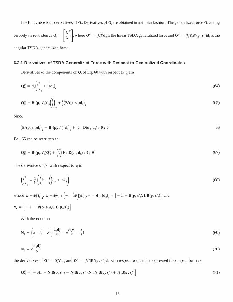
The focus here is on derivatives of Q i. Derivatives of Q j are obtained in a similar fashion. The generalized force Q i acting

on body i is rewritten as Q i � �QF

QN�, where QF � (f�l)dij is the linear TSDA generalized force and QN � (f�l)BT(pi, si)dij is the

angular TSDA generalized force.

6.2.1 Derivatives of TSDA Generalized Force with Respect to Generalized Coordinates

Derivatives of the components of Q i of Eq. 60 with respect to q are

QFq � dij�fl�

q

�fl�dij

�q

(64)

QNq � BT(pi, s i)dij�fl�

q

�fl�BT(pi, s i)dij

�q

(65)

Since

�BT(pi, s i)dij�

q� BT(pi, s i)�dij

�q� �0 ; D(s i, dij) ; 0 ; 0� 66

Eq. 65 can be rewritten as

QNq � BT(pi, s i)QF

q ��fl��0 ; D(s i, dij) ; 0 ; 0� (67)

The derivative of f�l with respect to q is

�fl�

q

� 1l 2��k� f

l�ll q � cll

.

q� (68)

where ll q � dTij�dij�q, ll

.

q � dTijvq ��vT � l

.

ldT

ij��dij�q, v � d

.

ij, �dij�

q� �� I ,� B(pi, s i), I , B(pj, s j)�, and

vq � �� 0,� B(p.

i, s i), 0, B(p.

j, s j)�.

With the notation

N1 � �k� fl� c l

.

l�dijdT

ij

l 2 � cdijvT

l 2 �flI (69)

N2 � cdijdT

ij

l 2 (70)

the derivatives of QF � (f�l)dij and QN � (f�l)BT(pi, si)dij with respect to q can be expressed in compact form as

QFq � �� N1,� N1B(pi, si) � N2B(p

.i, si),N1, N1B(pj, sj) � N2B(p

.j, sj)� (71)

14

QNq � �� BT(pi,si)N1,� BT(p i,si)�N1B(pi,si) � N2B(p

.i,si)� �

flD�si,dij

�,

BT(pi,si)N1,BT(pi,si)�N1B(pj,sj) � N2B(p

.j,sj)��

(72)

6.2.2 Derivatives of TSDA Generalized Force with Respect to Generalized Velocities

The derivatives of components of Q i with respect to q. are

QFq. � dij�fl�

q.

(73)

QNq. � BT(pi, s i)dij�fl�

q.

� BT(pi, s i)QFq. (74)

Using the following expressions:

�fl�

q.

� 1l

fq. � c

ll.

q. (75)

l.� 1

ldT

ijv � 1l

dTij�r. j � B(p

.j, s j)pj � r

.i � B(p

.i, s i)pi� (76)

l.

q. �

dTij

l�� I ,� B(pi, s i), I , B(pj, s j)� (77)

in Eqs. 73 and 74, the desired derivatives are

QFq. � c

dijdTij

l 2�� I ,� B(pi, s i), I , B(pj, s j)� (78)

QNq. � cB(pi, s i)

dijdTij

l 2�� I ,� B(pi, s i), I , B(pj, s j)� (79)

7 NUMERICAL EXPERIMENTS

The kinematic and kinetic derivatives obtained in analytical form in this paper are verified using two examples, with

numerical efficiency compared with finite differences. The two mechanisms analyzed are in assembled configurations and

kinematically admissible values for the generalized velocities were used in computations.

7.1 Slider Crank

The first example is the one–degree–of–freedom spatial slider–crank mechanism of Fig. 6, consisting of three bodies

(slider, crank, and connecting rod) connected by four joints (revolute, spherical, universal, and translational) and a TSDA. The

crank has length l C � 2.0 m and the connecting rod has length l CR � 5.0 m. All three bodies have unit masses and inertias. The

TSDA has the following characteristic values: k � 10.0 N�m, l 0 � 5.0 m, c � 1.0 Ns�m. The mechanism is described by 21

15

generalized coordinates, constrained by 17 joint constraints and 3 Euler parameter normalization constraints. The following

kinematic derivatives are considered: �q, ��Tq��q, ��qq

. �q, �q, and �q

. , where � is the array of constraint expressions, � is the

array of Lagrange multipliers, and � � ��qq. �

qq. is the right side of the acceleration constraint equation.

Table 1 presents maximum absolute differences between analytical and numerical values of the kinematic derivatives, for

different values of the perturbation � used in computing finite differences. Analytical Jacobians of generalized force with

respect to generalized coordinates and velocities are also compared to numerical Jacobians obtained with finite differences.

Results are presented in Table 2. Finite difference numerical derivatives are obtained with an accuracy of the order of the

perturbation �. As shown in Tables 1 and 2, they converge to the analytical values as � decreases.

As numerical results show, the perturbation � has a strong influence on computational accuracy using finite differences.

Moreover, selection of� to obtain derivatives within a prescribed accuracy is function of the type of derivative to be computed

and is problem dependent.

Availability of analytical derivatives not only gives more accurate results, but also leads to increased computational

efficiency. Table 3 presents the average CPU seconds required to compute the complete three groups of derivatives (kinematic

derivatives, generalized force derivatives, and generalized mass matrix derivatives) for the slider crank mechanism, using both

analytical and finite difference methods. The numerical experiments were performed on a HP J–210 computer. Speed–ups of

more than 10 were obtained for all derivative computations when using exact analytical formulas.

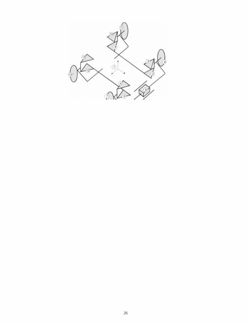
7.1 Fourteen Body Vehicle Model

As a second example consider the 14–body, eleven–degree–of–freedom model of the Army High Mobility Multipurpose

Wheeled Vehicle (HMMWV) shown in Fig. 7. Detailed data for this model can be found in Serban et. al. (1998). The same

tests carried out for the slider–crank mechanism were performed on this larger model, which consists of 14 bodies connected

by 21 joints (8 revolute, 8 spherical, 4 distance constraints, and 1 translational). The resulting model has 98 generalized

coordinates, 73 joint constraints and 14 Euler parameter normalization constraints. The 73 kinematic joint constraints used to

described this model translate into the following basic constraints: 16 spherical constraints, 4 distance constraints, 19 DOT–1

constraints, and 2 DOT–2 constraints. Table 4 presents maximum absolute differences between analytical and numerical

values of the kinematic derivatives, while Table 5 presents a comparison of results for generalized force Jacobians.

For this larger model the computation times obtained when using analytical derivative computations, as opposed to finite

differences, are presented in Table 6. Speed–ups are even larger than those obtained for the slider–crank example. Analytical

computation of kinematic and generalized force derivatives were about 30 times as fast as finite difference computations,

while the speed–up obtained in generating the generalized mass matrix derivatives was about 130.

16

8 CONCLUSIONS

Results presented in this paper enable accurate and efficient computation of higher order derivatives required in multibody

analysis, including implicit numerical integration of the differential–algebraic equations (DAE) of motion, dynamic

sensitivity analysis of mechanical systems, design optimization, and parameter estimation. A formulation to generate three

derivatives of the terms involved in the DAE of motion required in each of these analyses is presented and verified. This

formulation is extendable to compute higher order derivatives that appear in continuation methods for mapping workspace

boundaries. Derivative computations are developed in the Cartesian coordinate formulation with Euler parameters as

orientation parameters. Similar methods can be applied to generate kinematic and kinetic derivatives when using joint (or

relative) coordinates.

ACKNOWLEDGMENT

This research was supported by the US Army Tank–Automotive Command (TACOM), through the Automotive Research

Center (Department of Defense contract number DAAE07–94–R094).

REFERENCES

Adkins, F.A., 1996, “Numerical Continuation and Bifurcation Methods for Mechanism Workspace and Controllability Analysis,”

Ph.D. dissertation, The University of Iowa

Bestle, D. and Eberhard, P., 1992, “Analyzing and Optimizing Multibody Systems,” Mechanics of Structures and Machines, Vol

20(1), pp. 67–92

Bestle, D. and Seybold, J., 1992, “Sensitivity Analysis of Constrained Multibody Systems,” Archive of Applied Mechanics, Vol. 62,

pp. 181–190

Bischof, C., Roh, L., and Mauer, A., 1996, “ADIC: A Tool for the Automatic Differentiation of C Program,” Technical Report,

Mathematics and Computer Science Division, Argonne National Laboratory

Brenan, K.B., Campbell S.L., and Petzold L.R., 1989, Numerical Solution of Initial–Value Problems in Differential–Algebraic

Equations, North Holland Publishing Co., New York

Chang, C.O. and Nikravesh, P.E., 1985, “Optimal Design of Mechanical Systems With Constraint Violation Stabilization Method,”

Journal of Mechanisms, Transmissions, and Automation in Design, Vol. 107, pp. 493–498

Freudenstein, F. and Primerose, E.J., 1984, “On the Analysis and Synthesis of the Workspace of a three–Link, Turning–Pair

Connected Robot Arm,” Journal of Mechanisms, Transmissions, and Automation in Design, Vol. 106, pp. 365–370

17

Hairer E. and Wanner G., 1996, Solving Ordinary Differential Equations II: Stiff and Differential–Algebraic Problems, Springer–

Verlag, Berlin

Haug, E.J., 1987, “Design Sensitivity Analysis of Dynamic Systems,” Computer–Aided Design: Structural and Mechanical Systems,

C.A. Mota–Soares, Ed., Springer–Verlag, Berlin

Haug, E.J., 1989, Computer–Aided Kinematics and Dynamics of Mechanical Systems, Volume I: Basic Methods, Allyn and Bacon,

Needham Heights, Massachusetts

Haug, E.J. and Ehle, P.E., 1982, “Second–Order Design Sensitivity Analysis of Mechanical System Dynamics,” International

Journal for Numerical Methods in Engineering, Vol. 18, pp. 1699–1717

Haug, E.J., Luh, C.M., Adkins, F.A., and Wang, J.Y., 1996, “Numerical Algorithms for Mapping Boundaries of Manipulator

Workspaces,” Journal of Mechanical Design, Vol. 118, pp. 228–234

Haug, E.J., Negrut, D, and Iancu, M., 1997, “An Implicit Numerical Integration Algorithm for Differential–Algebraic Equations of

Multibody Dynamics,” Mechanics of Structures and Machines, to appear

Haug, E.J., Iancu, M, and Negrut, D., 1997, “Implicit Integration of the Equations of Multibody Dynamics in Descriptor Form,”

Submitted to the 1997 ASME Design Automation Conference

Jo, D.Y. and Haug, E.J., 1989, “Workspace Analysis of Multibody Mechanical Systems Using Continuation Methods,” Journal of

Mechanisms, Transmissions, and Automation in Design, Vol. 3, pp. 581–589

Krishnaswami, P., Wehage, R.A. and Haug, E.J., 1983, “Design Sensitivity Analysis of Constrained Dynamic Systems by Direct

Differentiation,” Technical Report No. 83–5, Center for Computer–Aided Design, The University of Iowa, Iowa City, Iowa

Litvin, F.L., 1980, “Application of Theorem of Implicit Function System Existence for Analysis and Synthesis of Linkages,”

Mechanism and Machine Theory, Vol. 15, pp. 115–125

Nikravesh, P.E., 1988, Computer–Aided Analysis of Mechanical Systems, Prentice–Hall, Englewood Cliffs, New Jersey

Potra, F.A., 1994, “Numerical Methods for Differential–Algebraic Equations with Application to Real–Time Simulation of

Mechanical Systems,” ZAMM, Vol. 74(3), pp. 177–187

Serban, R., Negrut, D., and Haug, E.J., 1998, “High Mobility Multipurpose Wheeled Vehicle (HMMWV) Multibody Models,”

Technical Report No. R–211, Center for Computer–Aided Design, The University of Iowa, Iowa City, Iowa

Tsai, Y.C. and Soni, A.H., 1981, “Accesible Region and Synthesis of Robot Arms,” Journal of Mechanical Design, Vol. 103, pp.

803–811

Wang, J.Y. and Wu, J.K., 1993, “Dextrous Workspace of Manipulators, Part II: Computational MEthods,” Mechanics of Structures

and Machines, Vol 21(4), pp. 471–506

18

Yang, F.C. and Lee, T.W., 1983, “On the Workspace of Mechanical Manipulators,” Journal of Mechanisms, Transmissions, and

Automation in Design, Vol. 105, pp. 62–69

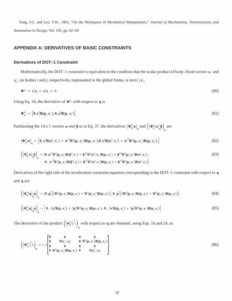
APPENDIX A: DERIVATIVES OF BASIC CONSTRAINTS

Derivatives of DOT–1 Constraint

Mathematically, the DOT–1 constraint is equivalent to the condition that the scalar product of body–fixed vectors si� and

sj�, on bodies i and j, respectively, represented in the global frame, is zero; i.e.,

�d1 � sT

i sj � sTj si � 0 (80)

Using Eq. 16, the derivative of �d1 with respect to q is

�d1q � �0, sT

j B(pi, si�), 0, sTi B(pj, sj�)� (81)

Partitioning the 14�1 vectors � and � as in Eq. 37, the derivatives ��d1q ��

q and ���d1

q ��

q��

q are

��d1q ��

q� �0, sT

j B(�2, si�) � �4TBT(pj, sj�)B(pi, si�),0, sT

i B(�4, sj�) � �2TBT(pi, si�)B(pj, sj�),� (82)

���d1q ��

q��

q� [0 ,�4TBT(pj,sj�)B(�2,si�) � �

4TBT(�4,sj�)B(pi,si�) � �4TBT(pj,sj�)B(�2,si�) ,

0 , �2TBT(pi,si�)B(�4,sj�)� �2TBT(�2,si�)B(pj,sj�) � �

2TBT(pi,si�)B(�4,sj�)�(83)

Derivatives of the right side of the acceleration constraint equation corresponding to the DOT–1 constraint with respect to q

and q. are

���d1q q

. �qq. �

q� [0 ,p

. Tj�2BT(p j,sj�)B(p

.i,si�) � BT(p

.j,sj�)B(pi,si�)� ,0 ,p

. Ti�2BT(pi,si�)B(p

.j,sj�) � BT(p

.i,si�)B(pj,sj�)�� (84)

���d1q q

. �qq. �

q.� � 0 , 2sT

j B(p.

i,si�) � 2p. T

j BT(pj,sj�)B(pi,si�) , 0 , 2sT

i B(p.

j,sj�) � 2p. T

i BT(pi,si�)B(pj,sj�)� (85)

The derivative of the product ���d1q�T��

q

with respect to q are obtained, using Eqs. 16 and 24, as

���d1q�T��

q

�� ��

00

00

0D(si�,sj)

0BT(pj,sj�)B(pi,si�)

00

00

0BT(pi,si�)B(pj,sj�)

0D(sj�,si)

��

�(86)

19

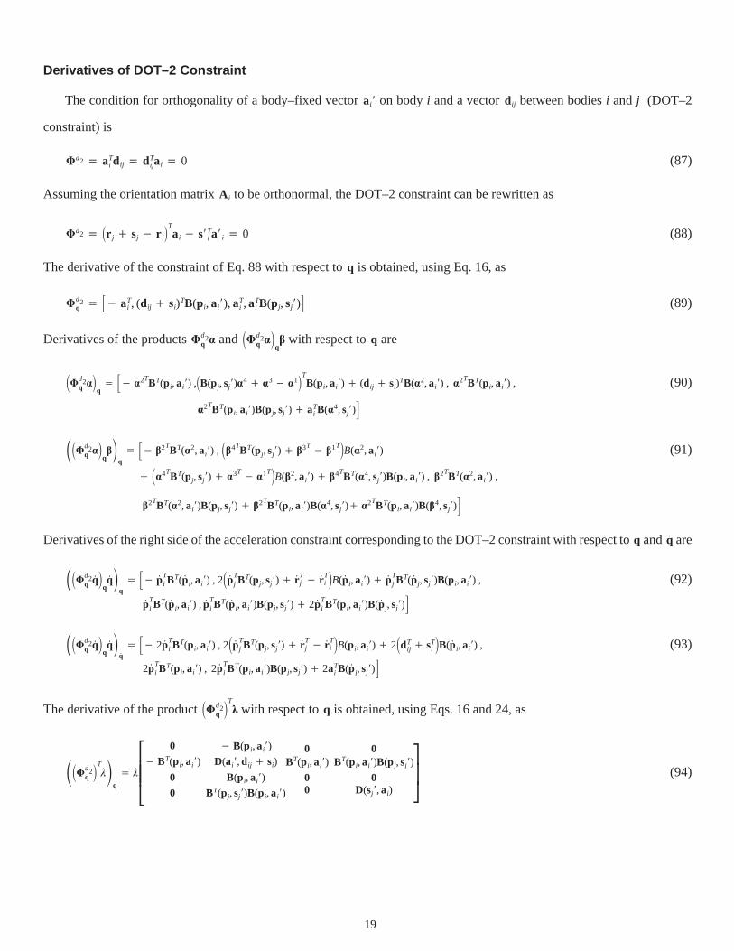
Derivatives of DOT–2 Constraint

The condition for orthogonality of a body–fixed vector ai� on body i and a vector dij between bodies i and j (DOT–2

constraint) is

�d2 � aT

i dij � dTijai � 0 (87)

Assuming the orientation matrix A i to be orthonormal, the DOT–2 constraint can be rewritten as

�d2 � �r j � sj � r i

�Tai � s�Ti a� i � 0 (88)

The derivative of the constraint of Eq. 88 with respect to q is obtained, using Eq. 16, as

�d2q � �� aT

i , (dij � si)TB(pi, ai�), aTi , aT

i B(pj, sj�)� (89)

Derivatives of the products �d2q � and ��d2

q ��

q� with respect to q are

��d2q ��

q� �� �

2TBT(pi,ai�) ,�B(p j,sj�)�4 � �

3 � �1�TB(pi,ai�) � (dij � si)

TB(�2,ai�) , �2TBT(pi,ai�) ,

�2TBT(pi,ai�)B(pj,sj�) � aT

i B(�4,sj�)�

(90)

���d2q ��

q��

q� �� �

2TBT(�2,ai�) , ��4TBT(pj,sj�) � �3T � �

1T�B(�2,ai�)

� ��4TBT(pj,sj�) � �3T � �

1T�B(�2,ai�) � �4TBT(�4,sj�)B(pi,ai�) , �2TBT(�2,ai�) ,

�2TBT(�2,ai�)B(pj,sj�) � �

2TBT(pi,ai�)B(�4,sj�)� �2TBT(pi,ai�)B(�4,sj�)�

(91)

Derivatives of the right side of the acceleration constraint corresponding to the DOT–2 constraint with respect to q and q. are

���d2q q

. �qq. �

q� �� p

. Ti B

T(p.

i,ai�) , 2�p. Tj B

T(pj,sj�) � r. Tj � r

. Ti �B(p

.i,ai�) � p

. Tj B

T(p.

j,sj�)B(pi,ai�) ,

p. T

i BT(p

.i,ai�) ,p

. Ti B

T(p.

i,ai�)B(pj,sj�) � 2p. T

i BT(pi,ai�)B(p

.j,sj�)�

(92)

���d2q q

. �qq. �

q.� �� 2p

. Ti B

T(pi,ai�) , 2�p. Tj B

T(pj,sj�) � r. Tj � r

. Ti �B(pi,ai�) � 2�dT

ij � sTi�B(p

.i,ai�) ,

2p. T

i BT(pi,ai�) , 2p

. Ti B

T(pi,ai�)B(pj,sj�) � 2aTi B(p

.j,sj�)�

(93)

The derivative of the product ��d2q�T

� with respect to q is obtained, using Eqs. 16 and 24, as

���d2q�T��

q

� �

�

0� BT(pi,ai�)

0

0

� B(pi,ai�)D(ai�,dij � si)

B(pi,ai�)BT(p j,sj�)B(p i,ai�)

0BT(pi,ai�)

00

0BT(pi,ai�)B(pj,sj�)

0D(sj�,ai)

�

(94)

20

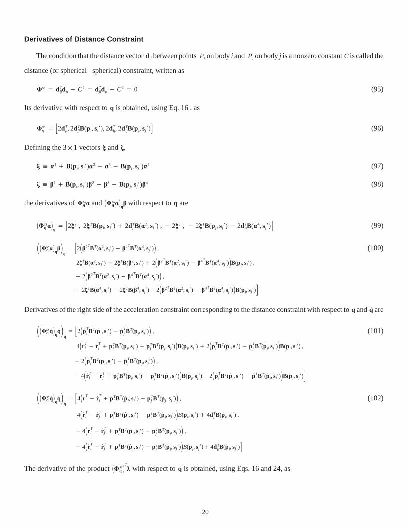
Derivatives of Distance Constraint

The condition that the distance vector dij between points Pi on body i and Pj on body j is a nonzero constant C is called the

distance (or spherical– spherical) constraint, written as

�ss� dT

ijdij � C2 � dTjidji � C2 � 0 (95)

Its derivative with respect to q is obtained, using Eq. 16 , as

�ssq � �2dT

ji, 2dTjiB(pi, si), 2dT

ij, 2dTijB(pj, sj)� (96)

Defining the 3�1 vectors � and �,

� � �1 � B(pi, si)�2 � �

3 � B(pj, sj)�4 (97)

� � �1 � B(pi, si)�2 � �

3 � B(pj, sj)�4 (98)

the derivatives of �ssq� and ��ss

q��q� with respect to q are

��ssq��q � �2�T , 2�TB(pi, si) � 2dT

jiB(�2, si) , � 2�T , � 2�TB(pj, sj) � 2dTjiB(�4, sj)� (99)

���ssq��q��q

� �2��2TBT(�2,si) � �4TBT(�4,sj)� ,

2�TB(�2,si) � 2�TB(�2,si) � 2��2TBT(�2,si) � �4TBT(�4,sj)�B(pi,si) ,

� 2��2TBT(�2,si) � �4TBT(�4,sj)� ,

� 2�TB(�4,si) � 2�TB(�4,sj)� 2��2TBT(�2,si) � �4TBT(�4,sj)�B(pj,sj)�

(100)

Derivatives of the right side of the acceleration constraint corresponding to the distance constraint with respect to q and q. are

���ssq q

. �qq. �

q� �2�p. T

i BT(p

.i,si) � p

. Tj B

T(p.

j,sj)� ,

� 2�p. Ti B

T(p.

i,si) � p. T

j BT(p

.j,sj)� ,

� 4�r. Ti � r

. Tj � pT

i BT(p

.i,si) � pT

j BT(p

.j,sj)�B(p

.j,sj)� 2�p. T

i BT(p

.i,si) � p

. Tj B

T(p.

j,sj)�B(pj,sj)�

4�r. Ti � r

. Tj � pT

i BT(p

.i,si) � pT

j BT(p

.j,sj)�B(p

.i,si) � 2�p. T

i BT(p

.i,si) � p

. Tj B

T(p.

j,sj)�B(pi,si) ,

(101)

���ssq q

. �qq. �

q.� �4�r. T

i � r. Tj � pT

i BT(p

.i,si) � pT

j BT(p

.j,sj)� ,

4�r. Ti � r

. Tj � pT

i BT(p

.i,si) � pT

j BT(p

.j,sj)�B(pi,si) � 4dT

jiB(p.

i,si) ,

� 4�r. Ti � r

. Tj � pT

i BT(p

.i,si) � pT

j BT(p

.j,sj)� ,

� 4�r. Ti � r

. Tj � pT

i BT(p

.i,si) � pT

j BT(p

.j,sj)�B(pj,sj)� 4dT

jiB(p.

j,sj)�

(102)

The derivative of the product ��ssq �

T� with respect to q is obtained, using Eqs. 16 and 24, as

21

�ssq �

T��

q� � �

�

2I2BT(pi,si�)

� 2I

� 2BT(pj,sj�)

2B(pi,si�)2D(si�,d ji) � 2BT(pi,si�)B(pi,si�)

� 2B(pi,si�)� 2BT(pj,sj�)B(pi,si�)

� 2I

� 2BT(p i,si�)

2I

2BT(p j,sj�)

� 2B(pj,sj�)

� 2BT(pi,si�)B(pj,sj�)

2B(pj,sj�)

2D(sj�,dij) � 2BT(pj,sj�)B(pj,sj�)

�

�(103)

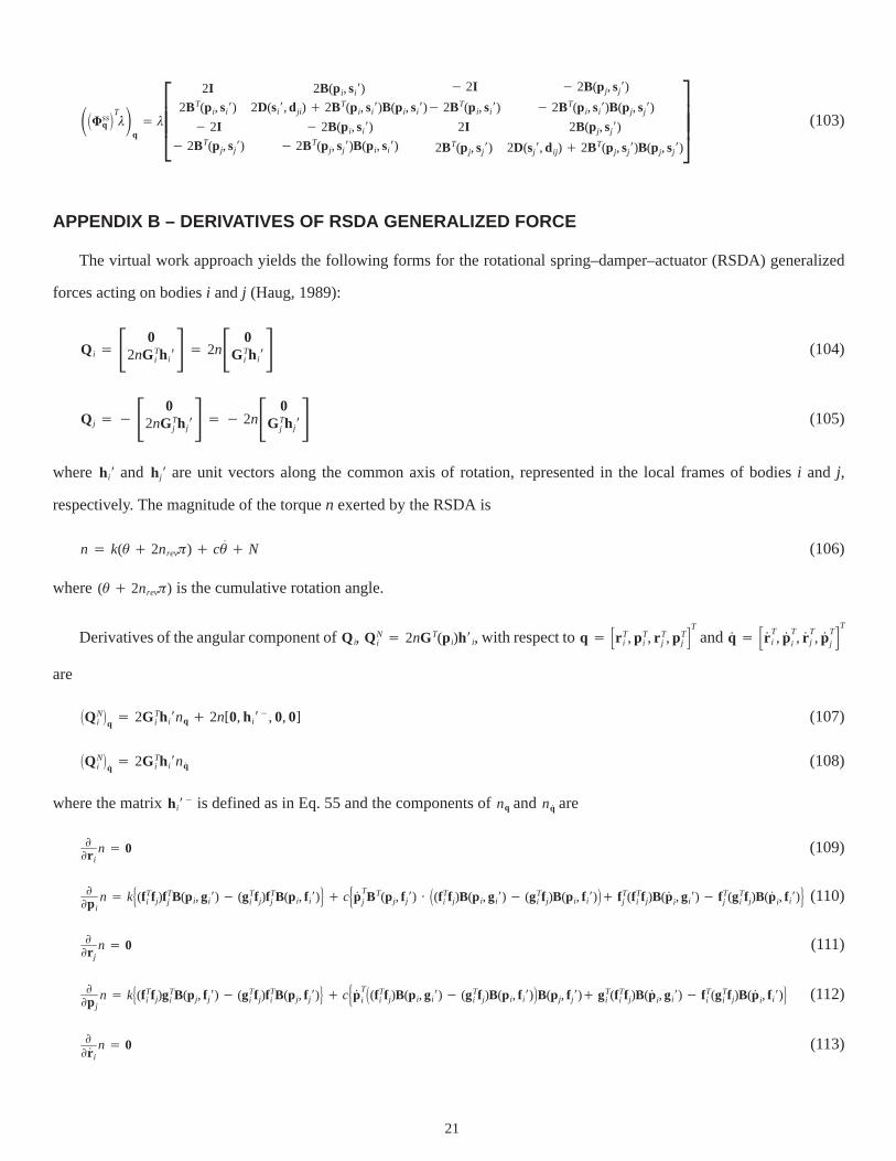
APPENDIX B – DERIVATIVES OF RSDA GENERALIZED FORCE

The virtual work approach yields the following forms for the rotational spring–damper–actuator (RSDA) generalized

forces acting on bodies i and j (Haug, 1989):

Q i � � 02nGT

i hi�� � 2n� 0GT

i hi�� (104)

Q j � �� 02nGT

j hj�� � � 2n� 0GT

j hj�� (105)

where hi� and hj� are unit vectors along the common axis of rotation, represented in the local frames of bodies i and j,

respectively. The magnitude of the torque n exerted by the RSDA is

n � k(�� 2nrev�) � c�.� N (106)

where (�� 2nrev�) is the cumulative rotation angle.

Derivatives of the angular component of Q i, QNi � 2nGT(pi)h� i, with respect to q � �r T

i , pTi , r T

j , pTj�T and q. � �r. T

i , p. T

i , r. T

j , p. T

j�T

are

QNi�q� 2GT

i hi�nq � 2n[0, hi��, 0, 0] (107)

QNi�q. � 2GT

i hi�nq. (108)

where the matrix hi�� is defined as in Eq. 55 and the components of nq and nq. are

��r i

n � 0 (109)

��p i

n � k�(fTi f j)f

Tj B(pi,gi�) � (gT

i f j)fTj B(pi, f i�) � c�p. T

j BT(pj, f j�) � (fT

i f j)B(p i,gi�) � (gTi f j)B(pi, f i�)�� fT

j (fTi f j)B(p

.i,gi�) � fT

j (gTi f j)B(p

.i, f i�) (110)

��r j

n � 0 (111)

��p j

n � k�(fTi f j)g

Ti B(pj, f j�) � (gT

i f j)fTi B(pj, f j�) � c�p. T

i(fT

i f j)B(pi,gi�) � (gTi f j)B(pi, f i�)�B(pj, f j�)� gT

i (fTi f j)B(p

.i,gi�) � fT

i (gTi f j)B(p

.i, f i�) (112)

��r

.in � 0 (113)

22

��p

.in � c�(fT

i f j)fTj B(pi,gi�) � (gT

i f j)fTj B(pi, f i�)� (114)

��r

.jn � 0 (115)

��p

.jn � c�(fT

i f j)gTi B(pj, f j�) � (gT

i f j)fTi B(pj, f j�)� (116)

In Eqs. 109 and 113, { f i, gi, hi} and �f j, gj, hj� are unit vectors along axes of the local frames on bodies i and j, respectively.

Derivatives of the angular component of Q j, QNj � � 2nGT(pj)h� j, with respect to q and q. are computed in a similar way.

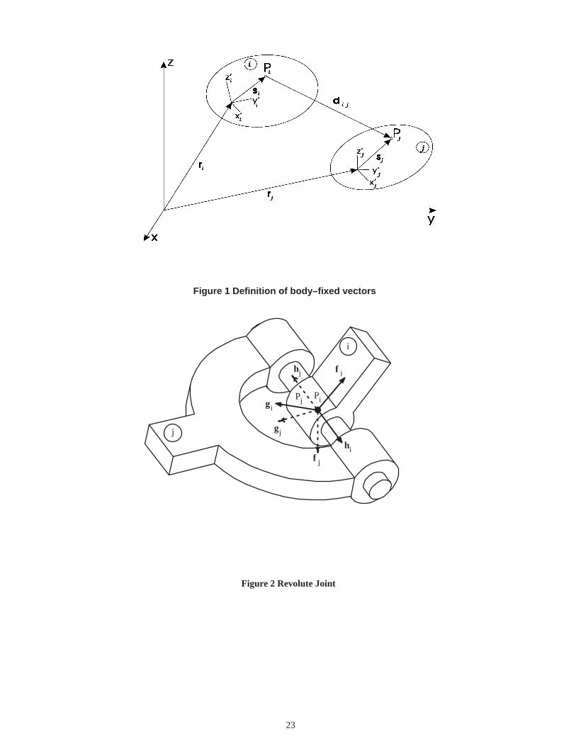
23

Figure 1 Definition of body–fixed vectors

hi

f i

gi

gj

f j

hj

i

j

PiPj

Figure 2 Revolute Joint

24

j

hi

f i

gi

hj

f j

gj

i

Pi Pj

Figure 3 Universal Joint

i

j

hi

gj

hj

f i

f j

gi dij

Pj

Pi

Figure 4 Translational Joint

25

Figure 5 Translational spring–damper–actuator

Figure 6 Spatial Slider–Crank Mechanism

26