
MRTC Report - Seoul National University
84
MRTC Report no.119/2004 ISSN 1404-3041 ISRN MDH-MRTC—119/2004-1-SE MRTC Report www.mrtc.mdh.se
Transcript of MRTC Report - Seoul National University

MRTC Report no.119/2004
ISSN 1404-3041 ISRN MDH-MRTC—119/2004-1-SE
MRTC Report
www.mrtc.mdh.se

TTaabbllee ooff CCoonntteennttss European Summer School on Embedded Systems
Sweden 2003
Period 1 (Low-power systems): July 14 - August 15, 2003
Energy Aware Computing: Analysis, Optimization and Upcoming Challenges………..1
Diana Marculescu (Carnegie Mellon University)
Energy-Efficient Scheduling for Hard Real-Time Applications on Dynamic Voltage
Supply Processors…………………………………………………………………....5 Flavius Gruian (Lund University)
Dynamic Voltage Scaling for Hard Real-Time Systems………………………………..9 Jihong Kim (Seoul National University)
Designing Energy Aware Systems…………………………………………………….12 Vijaykrishnan Narayanan (Pennsylvania State University)
Analysis and Optimization of Power Consumption for an ARM7-based Multimedia Handheld Device………………………………………………………16 Wonyong Sung (Seoul National University)
A Cycle-Accurate Joulemeter for CMOS VLSI Circuits……………………………...20 Soo-Ik Chae (Seoul National University)
Event-Driven Energy Characterization………………………………………………..24 Frank Bellosa (University of Erlangen)
Operating System Design for Energy Management…………………………………..29 Carla Ellis (Duke University)
i

Period 2 (Embedded systems): August 18 - Sept. 19, 2003
Modeling and Optimization of Embedded Systems using Constraint………………...33
Programming Krzysztof Kuchcinski (Lund University)
Embedded Systems Computer Architecture…………………………………………..37
Jakob Engblom (Virtutech/Uppsala University) Compilation for Embedded Processors………………………………………………..41
Daniel Kastner (AbsInt) Full-System Simulation……………………………………………………………….45
Jakob Engblom (Virtutech/Uppsala University) Communications and Networking in Embedded Systems…………………………….49
Ben Lee (Oregon State University) System-Level Optimization based on Genetic Algorithms……………………………53
Marcus Schmitz
ii
Period 3 (Real-time systems): Sept. 22 - Oct. 8, 2003
Predictability of Real-Time Software on Commodity Platforms……………………...57
Jane Liu (Microsoft) Elements of Real Time Systems………………………………………………………61
Lui Sha (University of Illinois)
The Timing Behavior of Embedded Systems: Specification, Prediction, and Checking…………………………………………………………………...………..63 Alan Shaw (University of Washington)
Stochastic Analysis of Real-Time Systems……………………………………………66
Kanghee Kim (Seoul National University) The Synchronous Programming Paradigm……………………………………………70
Nicolas Halbwachs and Pascal Raymond (Verimag) Formal Methods for Schedulability and Performance Analysis of Real-Time
Embedded Systems………………………………………………………………….74 Insup Lee (University of Pennsylvania)
Preemption Threshold Scheduling and Scenario-Based Multithreading of
UML-RT Models……………………………………………………………………77 Seongsoo Hong (Seoul National University)
iii
European Summer School on Embedded Systems, Sweden, 2003
1
Energy Aware Computing: Analysis, Optimization and Upcoming Challenges
Diana Marculescu, Member, IEEE
Abstract—Power dissipation has become a critical design
concern in recent years, driven by the increased levels of complexity and emergence of mobile applications. Embedded applications are not an exception to this trend and thus, are also very much affected by the increasing power consumption and cooling and packaging costs of existing platforms for embedded computing. While it is recognized that power consumption has become the limiting factor in keeping up with increasing performance trends, static or point solutions for power reduction are prone to reach their limits eventually. The paradigm of energy aware computing is thus intended to fill the gap between gate/circuit-level and system level power management techniques, by providing more power management levels and application-driven adaptability in the context of using multiple or dynamically adjustable voltages and local speeds. No less important are the challenges imposed by emerging platforms and technologies in the area of low power and energy aware computing. As a driver application, we consider wide-area computing substrates for ambient intelligent systems which provide an unexplored hardware platform for executing distributed applications under strict energy constraints. A new dimension in requirements, is that of reliability in the presence of runtime failures, thus paving the ground for achieving Dynamic Fault-Tolerance Management (DFTM) in addition to classic dynamic power management. Solutions to some of the emerging issues will be presented, along with open questions and directions for future research.
Index Terms—energy aware computing, fault tolerance, low power design.
I. INTRODUCTION
Power consumption has become the limiting factor not only for portable, embedded applications but also for
high-performance or desktop systems. While there has been notable growth in the use and application of these systems, their design process has become increasingly difficult due to the increasing design complexity and shortening time-to-market. The key factor in the design process of these systems is the issue of efficient power-performance estimation that can guide the system designer to make the right choice among several candidate architectures that can run a set of selected applications.
As important as the other levels of abstraction, the microarchitectural level presents additional challenges and
issues that need to be addressed. As such, one focus of this paper is on microarchitectural power analysis and optimization for core processors, characterized by either multimedia, or more general workloads. High-end and embedded processors are analyzed in the context of efficient design exploration for power-performance trade-off, as well as their potential for application-driven adaptability for energy-aware computation.
Manuscript received February 10, 2004. This work was supported in part
by NSF CAREER Award no. CCR-008479, SRC under Contract no. 2001-HJ-898 and Grant no. 2002-RJ-1052G.
D. Marculescu is with Department of Computer and Electrical Engineering at Carnegie Mellon University, Pittsburgh, PA 15213 USA (phone: 412-268-1167; fax: 412-268-2859; e-mail: [email protected]).
Another alternative to exploit fine grain microarchitectural adaptation is to use globally asynchronous locally synchronous (GALS) architectures, which attempt to combine the benefits of both fully synchronous and asynchronous systems. A GALS architecture is composed of synchronous blocks that communicate with each other only on demand, using an asynchronous or mixed-clock communication scheme. Through the use of a locally generated clock signal within each individual domain, such architectures make it possible to take advantage of the industry-standard synchronous design methodology. Not requiring a global clock distribution network and de-skewing circuitry, such systems have important advantages when compared to their fully synchronous counterparts.
Finally, challenges imposed by emerging platforms or technologies, such as electronic textiles or Ambient Intelligent systems are poised to play an important role in next generation low power or energy aware systems. We will also discuss some of these challenges in this paper, and their implications on the future design flows and methodologies.
The paper is organized as follows: Section II provides an overview of various techniques for power modeling and optimization including techniques for fine grain power adaptation at microarchitectural level, while Section IV addresses the problem of upcoming challenges imposed by emerging platforms.
II. MICROARCHITECTURE-DRIVEN POWER ANALYSIS AND OPTIMIZATION
To characterize the quality (in terms of power and performance) of various microarchitectural configurations, we need to rely on a few metrics of interest. In the case of power consumption, most researchers have concentrated on estimating or optimizing energy per committed instruction (EPI) or energy per cycle (EPC). While in the case of embedded computer systems with tight power budgets some performance may be sacrificed for lowering the power consumption, in the case of high-performance processors this is not desirable, and solutions that jointly address the problem of low power and high performance are needed. To this end,

European Summer School on Embedded Systems, Sweden, 2003
2
the energy delay product per committed instruction (EDPPI), defined as EPI*CPI*Tcycle, has been proposed as a measure that characterizes both the performance and power efficiency of a given architecture. Such a measure can identify microarchitectural configurations that keep the power consumption to a minimum without significantly affecting the performance. In addition to classical metrics (such as EPC and EPI), this measure can be used to assess the efficiency of different power-optimization techniques and to compare different configurations as far as power consumption is concerned.
One of the most widely used microarchitectural power simulators for superscalar, out-of-order processors is Wattch, which has been developed using the infrastructure offered by SimpleScalar. SimpleScalar performs fast, flexible, and accurate simulation of modern processors that implement a derivative of the MIPS-IV architecture and support superscalar, out-of-order execution, which is typical for today’s high-end processors. The power estimation engine of Wattch is based on the SimpleScalar architecture, but in addition, it supports detailed cycle-accurate information for all modules, including datapath elements, memory and CAM (Content-Addressable Memory) arrays, control logic, and clock distribution network. Wattch uses activity-driven, parameterizable power models, and it has been shown to be within 10% accurate when compared against three different architectures.
For accurate estimates, the power models used for the datapath modules can be based on input-dependent macromodels. The input statistics are gathered by the underlying detailed simulation engine and used, together with technology-specific load capacitance values, to obtain power-consumption values. Assuming a combination of static and dynamic CMOS implementations, one can use a cycle-accurate power macromodeling approach for each of the units of interest:
),( ,mod1,modmod,mod kulekuleulekule VVFP −= (1)
where Pmodule,k is the power consumption of a given module during cycle k when input vector Vmodule,k-1 is followed by Vmodule, k .
Today’s superscalar, out-of-order processors pack a lot of complexity and functionality on the same die. Hence, design exploration to find high performance or power efficient configurations is not an easy task. As shown previously, some of the factors that have a major impact on the power/performance of a given processor are issue width, cache configuration, etc. However, as shown before, the issue window strongly impacts the power cost of a typical superscalar, out-of-order processor. The issue width (and corresponding number of functional units), instruction window size, as well as the pipeline depth have the largest impact as parameters in a design exploration environment.
Figure 1. The design exploration framework
A possible design exploration environment follows the flow in Figure 1. At the heart of the exploration framework is a fast microarchitectural simulator (estimate_metrics) that provides sufficiently accurate estimates for the metric of interest. Depending on the designer’s needs, this metric can be one of: CPI, CPI*Tcycle, EPI, or EDPPI, depending on whether a high performance or a joint high-performance and energy-efficient organization is sought. As shown in Figure 1, the exploration is performed for a set of benchmarks B, a set of possible issue widths I, instruction window sizes W, and a number of possible voltage levels N. For each pair (issue width, instruction window size), the stage latencies are estimated. If a balanced pipelined design is sought, the pipeline is further refined to account for this, and only one voltage level is assumed for the entire design. Otherwise, depending on the latencies of the different stages, up to N different voltages are assigned to different modules such that performance constraints are maintained, and the slowest stage dictates the operating clock frequency.
A. Efficient microarchitectural power simulation For a design exploration environment to be able to explore
many possible design configurations in a short period of time, it has to rely either on a smart methodology to prune the design space or on a fast, yet sufficiently accurate estimation tool for the metrics of interest.
The crux of the estimation speed-up methodology relies on a two-level simulation methodology: for critical parts of the code, an accurate, lower-level (but slow) simulation engine is invoked, whereas for non-critical parts of the application program, a fast, high-level, but less accurate simulation is performed. Following the principle “make the common case accurate,” ideal candidates for critical sections that should be modeled accurately are those pieces of code in which the application spends a lot of time, which have been called hotspots.
Example: Consider the collection of basic blocks in Figure 2, where edges correspond to conditional branches and the weight of each edge is proportional to the number of times that direction of the branch is visited.
1
4
2
3
5
6
7 8
9
1
4
2
3
5
6
7 8
9
Figure 2. An example of two hotspots design_explore (B, I, W, N) for each benchmark BN in B
for IW in I = (IW1, IW2,...,IWn) for WS in W = (WS1, WS2,...,WSm)
estimate_stage_latencies (IW, WS); if (balanced_pipeline) balance_stages (IW, WS); estimate_metrics (BN, IW, WS, 1); else estimate_metrics (BN, IW, WS, N);
Hotspots are collections of basic blocks that closely communicate one to another but are unlikely to transition to a basic block outside of that collection. In Figure 2, basic blocks 1-4 and 5-9 are part of two different hotspots that communicate infrequently to one another. As shown before, these hotspots satisfy nice locality properties not only
European Summer School on Embedded Systems, Sweden, 2003
3
temporally, but also in terms of the behavior of the metrics that characterize power efficiency and performance. Temporal locality, as well as the high probability of reusing internal variables, make hotspots attractive candidates for sampling metrics of interest over a fixed sampling window after a warm-up period that would take care of any transient regimes. Estimated metrics obtained via sampling can be reused when the exact same code is run again. Although different, such an approach is similar in some ways to power-estimation techniques for hardware IPs using hierarchical sequence compaction or stratified random sampling. In addition, the relative sequencing of basic blocks is preserved, and the use of a warm-up period ensures that overlapping of traces is not necessary. This is in contrast with synthetically constructing traces for evaluating performance and power consumption.
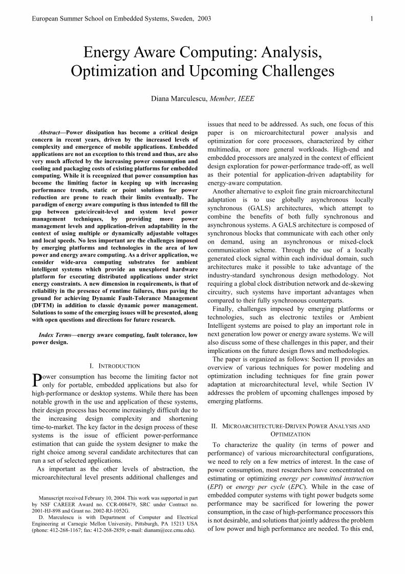
Figure 3. The two-level simulation engine To speed-up the simulation time inside the hotspots and
achieve the goal of “making the common case fast,” the sampling of power and performance metrics can be used until a given level of accuracy is achieved. This is supported by the fact that while being in a hotspot, both power consumption (EPC) and performance (IPC) achieve their stationary values within a short period of time, relative to the dynamic duration of the hotspot. As experimental evidence has shown, the steady-state behavior is achieved in less than 5% of the hotspot dynamic duration, thus providing significant opportunities for simulation speed-up, with minimal accuracy loss.
Figure 3 shows how the two-level simulation engine is organized. During detailed simulation, all performance and related power metrics are collected for cycle-accurate modeling. When a hotspot is detected, detailed analysis is continued for the entire duration of the sampling period. When sampling is done, the simulator is switched to basic profiling that only keeps track of the control flow of the application. Whenever the code exits the hotspot, detailed simulation is started again. This way, the error of estimation is conservatively bounded by the sampling error within the hotspots. Performing detailed simulation outside the hotspots ensures that the estimates are still accurate for benchmarks with low temporal locality (e.g., less than 60% time spent in hotspots).
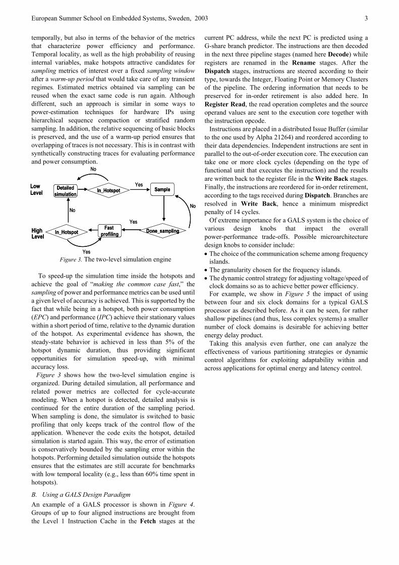
B. Using a GALS Design Paradigm An example of a GALS processor is shown in Figure 4. Groups of up to four aligned instructions are brought from the Level 1 Instruction Cache in the Fetch stages at the
current PC address, while the next PC is predicted using a G-share branch predictor. The instructions are then decoded in the next three pipeline stages (named here Decode) while registers are renamed in the Rename stages. After the Dispatch stages, instructions are steered according to their type, towards the Integer, Floating Point or Memory Clusters of the pipeline. The ordering information that needs to be preserved for in-order retirement is also added here. In Register Read, the read operation completes and the source operand values are sent to the execution core together with the instruction opcode.
Instructions are placed in a distributed Issue Buffer (similar to the one used by Alpha 21264) and reordered according to their data dependencies. Independent instructions are sent in parallel to the out-of-order execution core. The execution can take one or more clock cycles (depending on the type of functional unit that executes the instruction) and the results are written back to the register file in the Write Back stages. Finally, the instructions are reordered for in-order retirement, according to the tags received during Dispatch. Branches are resolved in Write Back, hence a minimum mispredict penalty of 14 cycles.
Yes
Yes
LowLevel
HighLevel
Detailedsimulation
Sample
Fast profiling
In_Hotspot
No
In_Hotspot Done_sampling
Yes
NoNo
Yes
Yes
LowLevel
HighLevel
Detailedsimulation
Sample
Fast profiling
In_Hotspot
No
In_Hotspot Done_sampling
Yes
NoNo
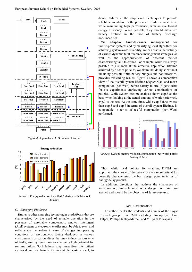
Of extreme importance for a GALS system is the choice of various design knobs that impact the overall power-performance trade-offs. Possible microarchitecture design knobs to consider include: • The choice of the communication scheme among frequency
islands. • The granularity chosen for the frequency islands. • The dynamic control strategy for adjusting voltage/speed of
clock domains so as to achieve better power efficiency. For example, we show in Figure 5 the impact of using
between four and six clock domains for a typical GALS processor as described before. As it can be seen, for rather shallow pipelines (and thus, less complex systems) a smaller number of clock domains is desirable for achieving better energy delay product.
Taking this analysis even further, one can analyze the effectiveness of various partitioning strategies or dynamic control algorithms for exploiting adaptability within and across applications for optimal energy and latency control.
European Summer School on Embedded Systems, Sweden, 2003
4
Figure 4. A possible GALS microarchitecture
Figure 5. Energy reduction for a GALS design with 4-6 clock domains
C. Emerging Platforms Similar to other emerging technologies or platforms that are
characterized by the need of reliable operation in the presence of unreliable components, ambient intelligent (AmI) systems or electronic textiles must be able to react and self-manage themselves in case of changes in operating conditions or environment. Being deployed in various environments or surroundings that may induce various type of faults, AmI systems have an inherently high potential for runtime failure. Such failures may range from intermittent electrical and mechanical failures at the system level, to
device failures at the chip level. Techniques to provide reliable computation in the presence of failures must do so while maintaining high performance, with an eye toward energy efficiency. When possible, they should maximize battery lifetime in the face of battery discharge non-linearities.
Via adaptive fault-tolerance management for failure-prone systems and by classifying local algorithms for achieving system-wide reliability, we can assess the viability of various dynamic fault tolerance management strategies, as well as the appropriateness of different metrics characterizing fault tolerance. For example, while it is always possible to just look at the effective application lifetime achieved by a set of policies, we claim that doing so without including possible finite battery budgets and nonlinearities, provides misleading results. Figure 6 shows a comparative view of the overall system lifetime (Figure 6(a)) and mean computation (per Watt) before battery failure (Figure 6(b)) for six experiments employing various combinations of policies. While system lifetime analysis shows exp.3 as the best, when looking at the actual amount of work performed, exp.7 is the best. At the same time, while exp.8 fares worse than exp.3 and exp.7 in terms of overall system lifetime, is comparable in terms of useful computation (per Watt) performed.
Energy reduction
02468
101214
ijpeg gc
cgz
ip vpr
mesa
equa
kepa
rser
vorte
xbz
ip2tur
b3d
avera
ge
[%]
6 clock domains5 clock domains4 clock domains
Figure 6. System lifetime vs. mean computation (per Watt) before
battery failure
Thus, while local policies for enabling DFTM are important, the choice of the metric is even more critical for correctly characterizing the best design point in terms of energy delay product.
In addition, directions that address the challenges of incorporating fault-tolerance as a design constraint are needed and should be the objective of future research.
ACKNOWLEDGMENT The author thanks the students and alumni of the Enyac
research group from CMU including: Anoop Iyer, Emil Talpes, Phillip Stanley-Marbell and V. Syam P. Rapaka.

Energy-Efficient Scheduling for Hard Real-TimeApplications on Dynamic Voltage Supply Processors
Flavius GruianDepartment of Computer Science
Lund UniversityBox 118, S-220 00 Lund, SwedenEmail: [email protected]
Abstract— The common energy reduction techniques implytrading performance for power, giving the impression thattimeliness and energy efficiency are opposing goals. However withthe advent of Dynamic Voltage Supply processors, even hard real-time systems can become energy efficient if adequate methods areemployed. This paper reviews several such scheduling techniques,addressing speed selection at both individual task and task grouplevel, applicable at run-time. Additionally, a couple of moreadvanced techniques, making use of run-time task variation arealso briefly presented.
I. INTRODUCTION
As the consumers demand more and more functionalityfrom their lap-tops, PDAs, cellular phones, other mobile de-vices, and household appliances, reducing the energy con-sumption becomes an essential issue for embedded systemsdesign. In this context, Dynamic Voltage Supply (DVS) pro-cessors seem to offer the best combination of flexibility andenergy efficiency. However, with the new dimension of pro-cessor speed (clock and supply voltage) introduced by these,special scheduling strategies are required to take full advantageof the available features. In the last couple of years the researchon dynamic voltage scheduling has flourished, becoming amature area, waiting for the consumer market to catch up. Thispaper reviews a number of such speed scheduling techniques,covering a rather wide spectrum of approaches from task togroup level, from static to dynamic methods, including morecomplex, probabilistic techniques. All of the strategies pre-sented in here exclusively address speed scheduling, withouttouching on compilation for low energy, power management,or low power communication. Furthermore, we focus on hardreal-time scheduling techniques.
The paper is organized as follows. Section II introduces thehardware support for speed scheduling, namely the DVS pro-cessor with its advantages and drawbacks. Speed schedulingmethods for both task and task group level are reviewed inSection III, which is the main part of the paper. Finally, wesummarize and conclude with Section IV.
II. HARDWARE SUPPORT
A wide variety of DVS processor systems are available todayon the market or as prototypes [1], [2], [4]–[6]. Although theirmain characteristic is the ability to adjust their speed (coreclock frequency and voltage) at run-time, different solutionsachieve this in various ways. The number of speed settings
is limited, varying between two (Intel SpeedStep) and tensof speeds (Transmeta Crusoe). Often these speed settings arenot on the same ideal delay-voltage curve, due to the discreteincrements for both voltage and clock frequency (Fig. 1).Furthermore, only some parts of the processor are able to
0.4
0.6
0.8
1
1.2
1.4
1.4 1.6 1.8 2 2.2 2.4 2.6 2.8 3
80200 speedsClock Energy (nJ)
Clock Length (ns)
Ideal charcteristics
Fig. 1. Measured data for Intel 80200 speed settings as energy–clock lengthpoints compared to ideal (non-discrete) characteristics. The circled setting isin fact obsolete, being covered by the point on the left.
operate at different speeds, while others, such as the I/O pads,need to satisfy certain standards. Additionally, a speed switchhas different characteristics for different processors or even fordifferent initial and final speeds. The most important in ourcase is arguably the switch latency, which spans from tensof µs to milliseconds. The limiting component is often theDelay Loop Logic (DLL) or Phase Lock Logic (PLL), whichtakes time to re-lock on the new clock frequency. However, theenergy overhead of a speed switch is usually very small, sincethe only active part during the switch is the clock generationlogic.
Common speed scheduling techniques make several simpli-fying assumptions, such as negligible overhead speed switchesand continuous range of speeds. These are not always limiting,and might become closer to reality with newer generations ofprocessors, as we briefly show later on.
III. SPEED SCHEDULING
Scheduling tasks for DVS processors implies both time andspeed setting (clock frequency and the corresponding supplyvoltage). For hard real-time systems the main requirement is
European Summer School on Embedded Systems, Sweden, 2003
5
keeping the deadlines, regardless of how fast the tasks canrun. In this context, good speed scheduling techniques takeadvantage of the idle times to slow down the processor speed,thus saving energy.
The large variation of speed scheduling methods makesit possible to classify them in different types. Dependingon the scheduling decisions, one can distinguish betweenoffline (static) and run-time (dynamic) or between operatingsystem level and user level approaches. Depending on the taskcharacteristics, one can find methods for fixed or variableexecution pattern, hard or soft deadlines. Depending on thelevel of intrusion, there are control flow aware approaches orinstance history sensitive techniques. Note that the distinctionsare not necessarily mutually exclusive, as typical approachesencountered in current research combine several of these fea-tures at different time moments or abstraction levels. Finally,one can distinguish also between intra-task (or task level)techniques, which are oblivious of the existence of other tasksin the system, and inter-task (or task-group level) techniques,which perform scheduling at system level. We review somerepresentative methods from the two different classes in thefollowing.
A. Intra-Task Approaches
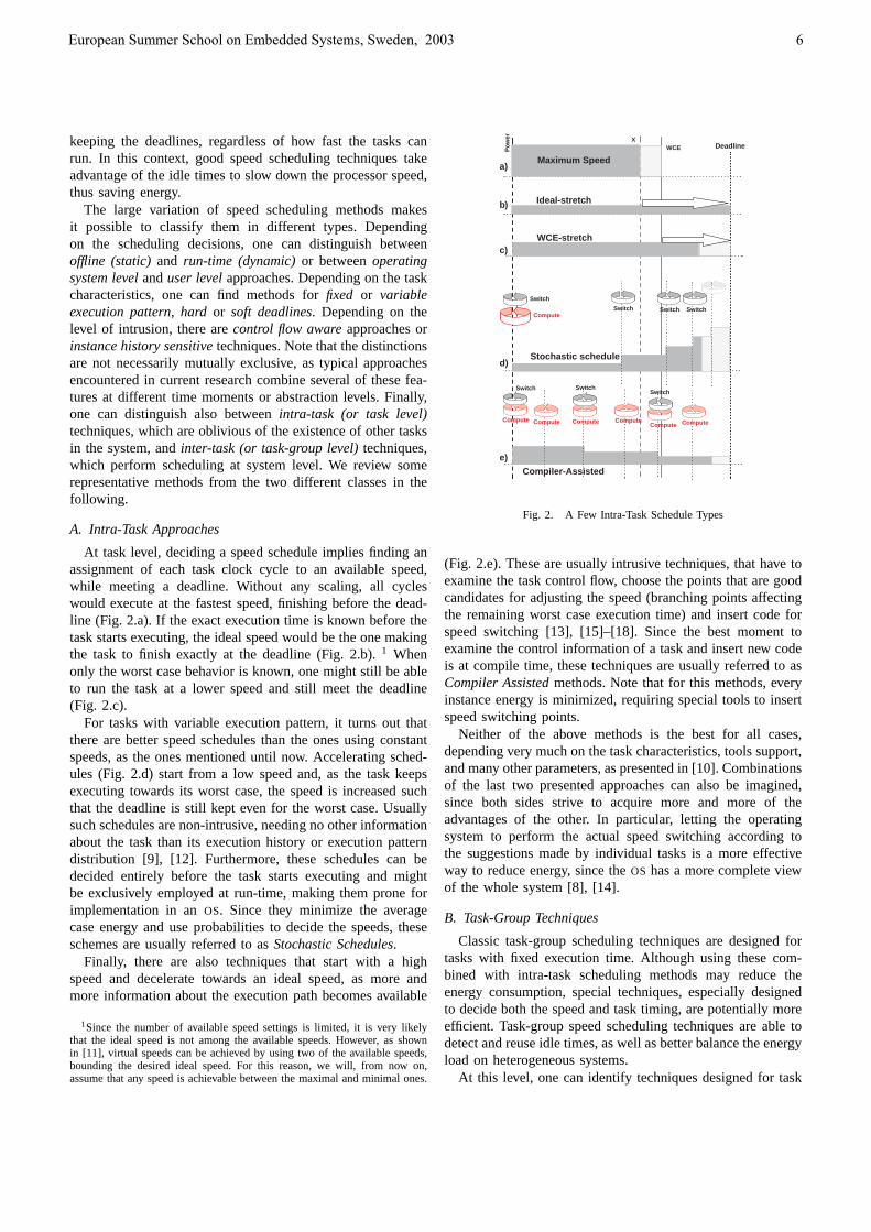
At task level, deciding a speed schedule implies finding anassignment of each task clock cycle to an available speed,while meeting a deadline. Without any scaling, all cycleswould execute at the fastest speed, finishing before the dead-line (Fig. 2.a). If the exact execution time is known before thetask starts executing, the ideal speed would be the one makingthe task to finish exactly at the deadline (Fig. 2.b). 1 Whenonly the worst case behavior is known, one might still be ableto run the task at a lower speed and still meet the deadline(Fig. 2.c).
For tasks with variable execution pattern, it turns out thatthere are better speed schedules than the ones using constantspeeds, as the ones mentioned until now. Accelerating sched-ules (Fig. 2.d) start from a low speed and, as the task keepsexecuting towards its worst case, the speed is increased suchthat the deadline is still kept even for the worst case. Usuallysuch schedules are non-intrusive, needing no other informationabout the task than its execution history or execution patterndistribution [9], [12]. Furthermore, these schedules can bedecided entirely before the task starts executing and mightbe exclusively employed at run-time, making them prone forimplementation in an OS. Since they minimize the averagecase energy and use probabilities to decide the speeds, theseschemes are usually referred to as Stochastic Schedules.
Finally, there are also techniques that start with a highspeed and decelerate towards an ideal speed, as more andmore information about the execution path becomes available
1Since the number of available speed settings is limited, it is very likelythat the ideal speed is not among the available speeds. However, as shownin [11], virtual speeds can be achieved by using two of the available speeds,bounding the desired ideal speed. For this reason, we will, from now on,assume that any speed is achievable between the maximal and minimal ones.
Switch
ComputeSwitch Switch Switch
Compute Compute Compute ComputeCompute Compute
Switch SwitchSwitch
WCEX
Deadline
Ideal-stretch
WCE-stretch
Stochastic schedule
Compiler-Assisted
Maximum Speeda)
b)
c)
d)
e)
Po
wer
Fig. 2. A Few Intra-Task Schedule Types
(Fig. 2.e). These are usually intrusive techniques, that have toexamine the task control flow, choose the points that are goodcandidates for adjusting the speed (branching points affectingthe remaining worst case execution time) and insert code forspeed switching [13], [15]–[18]. Since the best moment toexamine the control information of a task and insert new codeis at compile time, these techniques are usually referred to asCompiler Assisted methods. Note that for this methods, everyinstance energy is minimized, requiring special tools to insertspeed switching points.
Neither of the above methods is the best for all cases,depending very much on the task characteristics, tools support,and many other parameters, as presented in [10]. Combinationsof the last two presented approaches can also be imagined,since both sides strive to acquire more and more of theadvantages of the other. In particular, letting the operatingsystem to perform the actual speed switching according tothe suggestions made by individual tasks is a more effectiveway to reduce energy, since the OS has a more complete viewof the whole system [8], [14].
B. Task-Group Techniques
Classic task-group scheduling techniques are designed fortasks with fixed execution time. Although using these com-bined with intra-task scheduling methods may reduce theenergy consumption, special techniques, especially designedto decide both the speed and task timing, are potentially moreefficient. Task-group speed scheduling techniques are able todetect and reuse idle times, as well as better balance the energyload on heterogeneous systems.
At this level, one can identify techniques designed for task
European Summer School on Embedded Systems, Sweden, 2003
6
graphs, task sets, or hybrid models such as multi-rate graphs.Usually task graph methods are concerned with communi-cating tasks on multi-processor systems, with a unique rate,suitable for a static cyclic executive approach. On the otherhand, task set techniques emphasize timing (response times)on uni-processor systems, involving both static analysis andrun-time scheduling. Regardless of the model, the majority ofspeed scheduling approaches have both a static and a dynamic(run-time) part. Predominantly static techniques are easier toanalyze and derive, being however less flexible. Dynamicapproaches exhibit increased run-time overhead and are harderto analyze, but can adapt better to workload variations. In thiscontext, we start describing simple static scheduling methods(task graph based) and continue with more complex anddynamic methods (task set based).
1) Static Scheduling Methods: The simplest case is thatof uni-processor scheduling of a group of tasks with uniqueperiod and deadline. The ideal schedule in this case (analog toFig. 2.b and c) is the one with constant speed, finishing exactlyat the deadline. A similar method, named Proportional Stretch,can be applied to task-graph on multi-processors. First theseare scheduled using a classic technique (i.e. list-scheduling),and the resulting schedule is then proportionally stretch tothe deadline, reducing the speeds of all tasks with the samefactor. However this method is sub-optimal for heterogeneoussystems and schedules with slack on the non-critical path.
More specialized techniques are able to overcome theproblems mentioned above [22], [23]. The LENES approach,introduced in [19], is a list scheduling based algorithm, witha special energy-aware priority function. The start and end ofeach task are treated as separate graph nodes, being scheduledor delayed for a later time depending on the global energyof the partial schedule. With LENES, energy savings between10% and 28% off the non-scaling case can be achieved, evenfor the tightest possible schedule. Additionally, it is possibleto combine static speed scheduling with task to processormapping in an energy-aware system design flow, yieldingfurther energy reductions [21], [25].
2) Dynamic Scheduling Methods: For sets of tasks withdifferent rate, deadline and variable execution time staticmethods cannot handle the idle times (slack) that appears inthe system at run-time. In this case dynamic speed schedulingstrategies must be employed, usually built on top of clas-sic real-time scheduling techniques such as Rate-MonotonicScheduling (RMS) [32] or Earliest Deadline First (EDF) [33].The majority of these techniques employ both offline and run-time decisions. Offline procedures usually include assigningbounds to task speeds and response time analysis for differentrun-time strategies. Run-time decisions concern exact speedassignment and slack management. Some of such speed-related offline and run-time decisions are actually standalone,and can be easily plugged in the classic real-time strategies.
Deciding the Maximum Required Speeds (MRS) for RMS
[9], [26] and EDF [27], [30] is an offline analysis techniquethat can suggest the upper bound on each task speed, suchthat all the deadlines are met. However, at this point all tasks
are assumed to be running their worst case, and therefore anadditional run-time strategy would take advantage of the slackappearing from tasks running faster than their worst case.
A RMS-based run-time speed scheduling strategy for a two-speed processor is described in [24]. [26] presents an improvedmethod, that runs lone tasks as slow as possible until the arrivalof a next task instance. Fixed-priority scheduling has beenfurther investigated in [9], [29], [31].
The slack management strategy presented in [9] uses slacklevels to accumulate idle times, corresponding to priorities.Task instances can use slack from higher levels than theirown priority and produce lower priority slack if they finishearly. The approach was proven to keep the response timesfrom the classic RMS. Additionally, there are various waysto distribute the available slack to the instances about toexecute, such as Greedy, if the next instance uses all the slackand Mean Proportional, if the slack is distributed accordingto the expected execution time. Furthermore, this strategycan be combined with intra-task speed scheduling for higherefficiency. Following a similar approach, EDF-based speedscheduling techniques were also developed [27], [28], [30].
C. Advanced Methods
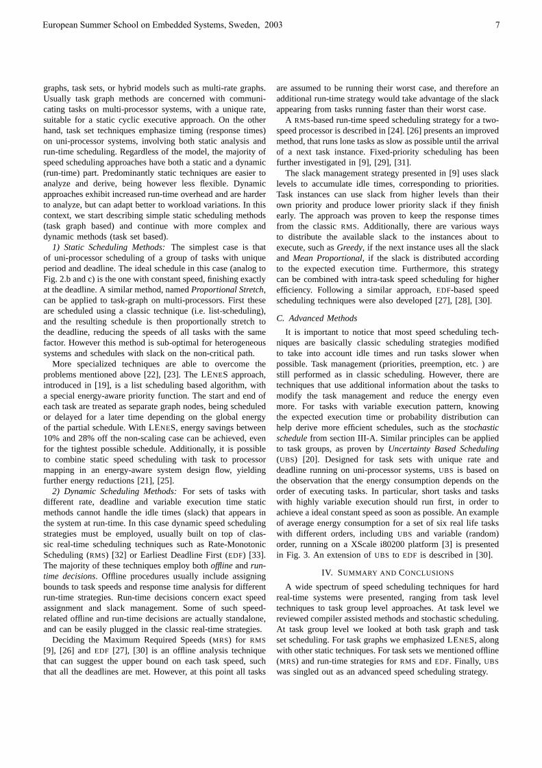
It is important to notice that most speed scheduling tech-niques are basically classic scheduling strategies modifiedto take into account idle times and run tasks slower whenpossible. Task management (priorities, preemption, etc. ) arestill performed as in classic scheduling. However, there aretechniques that use additional information about the tasks tomodify the task management and reduce the energy evenmore. For tasks with variable execution pattern, knowingthe expected execution time or probability distribution canhelp derive more efficient schedules, such as the stochasticschedule from section III-A. Similar principles can be appliedto task groups, as proven by Uncertainty Based Scheduling(UBS) [20]. Designed for task sets with unique rate anddeadline running on uni-processor systems, UBS is based onthe observation that the energy consumption depends on theorder of executing tasks. In particular, short tasks and taskswith highly variable execution should run first, in order toachieve a ideal constant speed as soon as possible. An exampleof average energy consumption for a set of six real life taskswith different orders, including UBS and variable (random)order, running on a XScale i80200 platform [3] is presentedin Fig. 3. An extension of UBS to EDF is described in [30].
IV. SUMMARY AND CONCLUSIONS
A wide spectrum of speed scheduling techniques for hardreal-time systems were presented, ranging from task leveltechniques to task group level approaches. At task level wereviewed compiler assisted methods and stochastic scheduling.At task group level we looked at both task graph and taskset scheduling. For task graphs we emphasized LENES, alongwith other static techniques. For task sets we mentioned offline(MRS) and run-time strategies for RMS and EDF. Finally, UBS
was singled out as an advanced speed scheduling strategy.
European Summer School on Embedded Systems, Sweden, 2003
7
0.1
0.2
0.3
0.4
0.5
0.6
0.7
0.8
0.9
00 0.01 0.02 0.03 0.04 0.05 0.06 0.07 0.08 0.09
Pow
er (
W)
Time (s)
UBS (21.11mJ)Reverse UBS (24.34mJ)
Random (22.78mJ)WCE-stretch (28.58mJ)
MAX (37.57mJ)
Fig. 3. Average power profile for six tasks on i80200, running accordingto different orders: UBS, its inverse order, variable order, minimal constantspeed to meet the deadline in all cases and maximal speed.
To conclude, it is most likely that very soon most processorswill be DVS processors. A large number of speed schedulingtechniques are already available out there, covering most ofthe situations or problem set-ups. Although improvements arepossible, expect further energy reductions to be minimal, sincethe nature of the problems requires larger and larger effortsfor rapidly decreasing results. However, examining the impactof speed scheduling techniques at system and even networklevel appears to be a tempting research area. Combiningtask management (migration, duplication) in wireless networkswith DVS techniques and power management seem to offereven more possibilities for energy reduction. Minimizing thespeed switching overhead is also a must, as the processorsbecome faster and faster.
REFERENCES
[1] T. D. Burd, T. A. Pering, A. J. Stratakos, and R. W. Brodersen. Adynamic voltage scaled microprocessor system. IEEE Journal of SolidState Circuits, 35(11), November 2000.
[2] T. A. Pering, T. D. Burd, and R. W. Brodersen. Voltage scheduling inthe lpARM microprocessor system. In Proc. of the 2000 ISLPED, pages96–101, 2000.
[3] ADI Engineering. 80200EVB Reference Platform.http://www.adiengineering.com/product80200EVB.html.
[4] AMD. AMD PowerNowTM Technology Dynamically Manages Powerand Performance, Rev. A, November 2000. Informational White PaperNo. 24404.
[5] M. Fleischmann. LongRun power management - dynamic power man-agement for crusoe processors. Technical report, Transmeta Corporation,January 17, 2001.
[6] Intel. Intel 80200 Processor based on Intel XScaleTM MicroarchitectureDatasheet, September 2001. Order Number: 273414-003.
[7] J. M. Rabaey and M. Pedram, editors. Low Power Design Methodolo-gies. Kluwer Academic Publishers, 1996.
[8] N. AbouGhazaleh, B. Childers, D. Mosse, R. Melhem, and M. Craven.Energy management for real-time embedded applications with compilersupport. In ACM SIGPLAN Langauges, Compilers,and Tools forEmbedded Systems (LCTES’03), 2003.
[9] F. Gruian. Hard real-time scheduling for low-energy using stochasticdata and dvs processors. In Proc. of the 2001 ISLPED, pages 46–51,August 6–7 2001.
[10] F. Gruian. On energy reduction in hard real-time systems containingtasks with stochastic execution times. In IEEE Workshop on PowerManagement for Real-Time and Embedded Systems, pages 11–16, May29 2001.
[11] T. Ishihara and H. Yasuura. Voltage scheduling problem for dynamicallyvariable voltage processors. In Proc. of the 1998 ISLPED, pages 197–202, 1998.
[12] J. R. Lorch and A. J. Smith. Improving dynamic voltage scalingalgorithms with PACE. In Proc. of ACM SIGMETRICS 2001, pages50–61, 2001.
[13] D. Shin, J. Kim, and S. Lee. Intra-task voltage scheduling for low-energy hard real-time applications. IEEE Design & Test of Computers,18(2), March-April 2001.
[14] Y. Shin, H. Kawaguchi, and T. Sakurai. Cooperative voltage scaling(CVS) between OS and applications for low-power real-time systems.In Proc. of the 2001 ICICC, pages 553–556, 2001.
[15] C.-H. Hsu and U. Kremer. Compiler-directed dynamic voltage scalingbased on program regions. Technical Report DCS-TR461, RutgersUniversity, November 2001.
[16] S. Lee and T. Sakurai. Run-time voltage hopping for low-power real-time systems. In Proc. of the 2000 DAC, pages 806–809, 2000.
[17] R. Melhem, N. AbouGhazaleh, H. Aydin, and D. Mosse. Power AwareComputing, chapter Power Management Points in Power-Aware Real-Time Systems. Plenum/Kluwer Publishers, 2002.
[18] D. Mosse, H. Aydin, B. Childers, and R. Melhem. Compiler-assisted dy-namic power-aware scheduling for real-time applications. In Workshopon Compilers and Operating Systems for Low-Power, October 2000.
[19] F. Gruian and K. Kuchcinski. LEneS: Task-scheduling for low-energysystems using variable voltage processors. In Proceedings of the 2001Asia South Pacific – Design Automation Conference, pages 449–455,January 30 – February 2 2001.
[20] F. Gruian and K. Kuchcinski. Uncertainty-based scheduling: Energy-efficient ordering of tasks with variable execution time. In InternationalSymposium on Low Power Electronics and Design (ISLPED’03), August2003.
[21] F. Gruian. System-level design methods for low-energy architecturescontaining variable voltage processors. In B. Falsafi and T.N. Vijayku-mar, editors, Lecture Notes in Computer Science, number 2008, pages1–12. Springer, 2000. First International Workshop on Power-AwareComputer Systems.
[22] J. Liu, P. H. Chou, N. Bagherzadeh, and F. Kurdahi. Power-awarescheduling under timing constraints for mission-critical embedded sys-tems. In Proceedings of the 38th Design Automation Conference, pages840–845, June 2001.
[23] J. Luo and N. K. Jha. Power-conscious joint scheduling of periodictask graphs and aperiodic tasks in distributed real-time systems. InProceedings of the 2000 IEEE/ACM ICCAD, pages 357–364, 2000.
[24] Y.-H. Lee and C. M. Krishna. Voltage-clock scaling for low energyconsumption in real-time embedded systems. In Proc. of the 6th ICRTCSA, pages 272–279, 1999.
[25] M. T. Schmitz, B. M. Al-Hashimi, and P. Eles. Energy-efficientmapping and scheduling for DVS enabled distributed embedded systems.In Proceedings of the 2002 Design, Automation and Test in EuropeConference and Exhibition, pages 514–521, 2002.
[26] Y. Shin and W. Choi. Power conscious fixed priority scheduling forreal-time systems. In Proc. of the 36th DAC, pages 134–139, 1999.
[27] F. Yao, A. Demers, and S. Shenker. A scheduling model for reducedCPU energy. IEEE Annual Foundations of CS, pages 374–382, 1995.
[28] R. Jejurikar and R. Gupta. Energy aware edf scheduling with tasksynchronization for embedded real time systems. Technical Report 02-24, CECS, UC Irvine, August 2002.
[29] R. Jejurikar and R. Gupta. Energy aware task scheduling with tasksynchronization for embedded real time systems. In Proc. of the 2002CASES, pages 164–169, 2002.
[30] F. Gruian. Energy-Centric Scheduling for Real-Time Systems. Doctoraldissertation, Lund University, December 2002. ISBN 91-628-5494-1,ISSN 1404-1219.
[31] G. Quan and X. Hu. Energy efficient fixed-priority scheduling for real-time systems on variable voltage processors. In Proceedings of the 2001Design Automation Conference, pages 828–833, 2001.
[32] J. Lehoczky, L. Sha, and Y. Ding. The rate monotonic scheduling algo-rithm: exact characterization and average case behavior. In Proceedingsof the 1989 Real Time Systems Symposium, pages 166–171, 1989.
[33] J. A. Stankovic, M. Spuri, K. Ramamritham, and G. C. Buttazzo. Dead-line Scheduling For Real-Time Systems: EDF and Related Algorithms.Kluwer Academic Publishers, 1998.
European Summer School on Embedded Systems, Sweden, 2003
8

European Summer School on Embedded Systems, Sweden, 2003 9
Dynamic Voltage Scaling for Hard Real-Time Systems
Jihong Kim, Member, IEEE
Abstract—Dynamic voltage scaling (DVS), which adjusts the
supply voltage and clock frequency dynamically, is an effective technique for designing low-power embedded real-time systems. In this lecture, we discuss recent DVS techniques at various design abstractions targeting for hard real-time systems. Following a brief introduction to low-power system design techniques in general, we cover DVS techniques from three software levels, the operating system level, the compiler level and the algorithm level. Experimental results show that DVS can achieve significant energy reductions in hard real-time systems.
Index Terms— dynamic voltage scaling, low power, hard real-time systems.
I. INTRODUCTION
Energy consumption is one of the most important design constraints in designing battery-operated embedded systems such as digital cellular phones and digital
cameras. For such systems, the energy consumption is a critical design factor because it directly affects the system’s lifetime. The dynamic energy consumption E, which currently dominates the total energy consumption of CMOS circuits, is given by E ∝ CL Ncycle VDD
2, where CL is the load capacitance, Ncycle is the number of executed cycles, and VDD is the supply voltage. Because the dynamic energy consumption E is quadratically dependent on the supply voltage VDD, lowering VDD is an effective technique in reducing the energy consumption. However, lowering the supply voltage also decreases the clock speed, because the circuit delay TD of CMOS circuits is given by TD ∝ VDD/(VDD − VT)α , where VT is the threshold voltage and α is a technology dependent constant [1]. When a given task does not require the maximum performance of a system, the clock speed (and its corresponding supply voltage) can be dynamically adjusted to the lowest possible level that still satisfies the task’s required performance. This is the key principle of the dynamic voltage scaling (DVS) technique [2]. With an ever-growing importance of the power/energy consumption in portable embedded systems, many DVS algorithms (e.g., [3]-[7]) have been proposed. At the same time, several commercial variable-voltage processors were developed as
well (e.g., Intel’s Xscale, AMD’s K6–2+, and Transmeta’s Crusoe processors).
Manuscript received January 31, 2004. This research was supported in
part by the Ministry of Education under the BK21 program and the University IT Research Center Project.
Jihong Kim is with the School of Computer Science & Engineering, Seoul National University, Seoul, Korea (phone: +82-2-880-8792; fax: +82-2-871-4912; e-mail: [email protected]).
A generic DVS algorithm consists of two steps, the slack (i.e., idle interval) estimation step and slack distribution step. The slack estimation step tries to identify as much slack times as possible while the slack distribution step aims to distribute the identified slack times in such a fashion that the resulting speed schedule is as uniform as possible. Slack times generally come from two sources; static slack times are the extra times available that can be identified statically, while dynamic slack times are caused from run-time variations of executions. In this lecture, we cover various DVS techniques proposed for hard real-time systems. For hard real-time systems, the goal of voltage scaling algorithms is to find an energy-efficient voltage schedule with all the stringent timing constraints satisfied. We cover DVS techniques from all three software layers, namely, the operating system level, compiler level, and algorithm level. The rest of this extended abstract is organized as follows. In Section Ⅱ, we describe the overall organization of the lecture and summarize the main topics of the lecture. Additional information on the presented topics is given in Section Ⅲ.
II. LECTURE ORGANIZATION
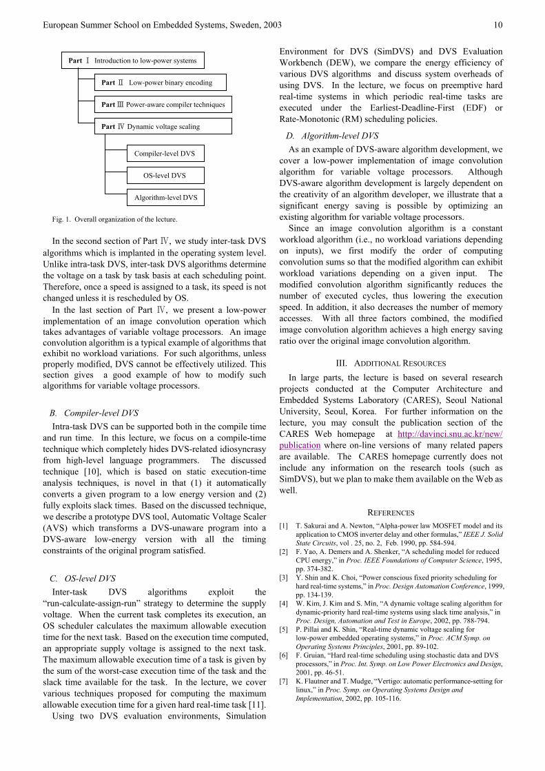
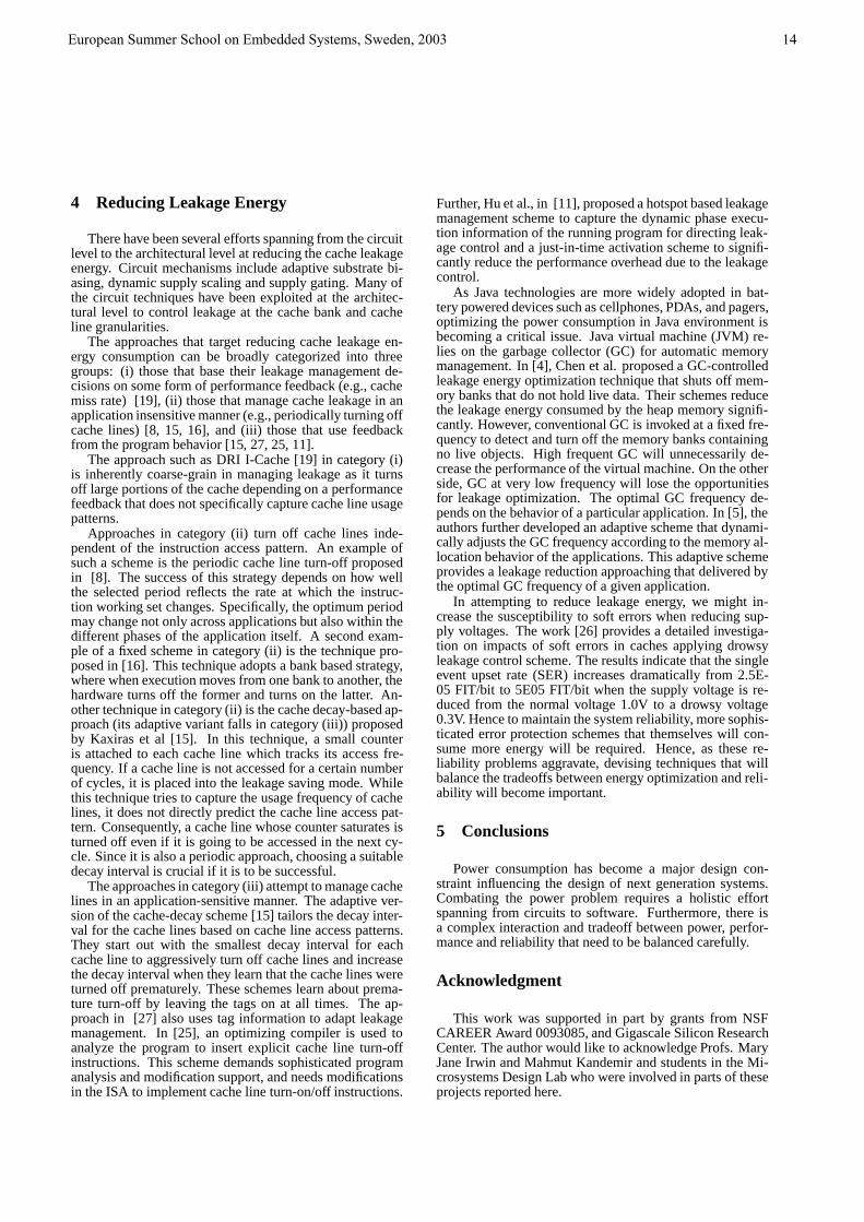
A. Overview of Lecture As shown in Figure 1, the lecture consists of four parts. In
Part Ⅰ, we review the main sources of power consumption in CMOS circuits and introduce the principle of power-aware software computing. In Parts Ⅱand Ⅲ, as concrete examples of the principle described in Part Ⅰ, we present several low-power techniques based on switching activity reduction and battery characteristics. They include low-power register relabelling techniques, operation rearrangement techniques for VLIW processors and battery-aware balanced modulo scheduling [8][9].
Part Ⅳ, which covers the main topic of this lecture, is organized in three sections. In the first section, we focus on intra-task DVS in which the supply voltage is adjusted within a task boundary. Since the execution speed is changed for a single task, intra-task DVS techniques are implemented in the compiler level.
European Summer School on Embedded Systems, Sweden, 2003 10
Fig. 1. Overall organization of the lecture. In the second section of Part Ⅳ, we study inter-task DVS
algorithms which is implanted in the operating system level. Unlike intra-task DVS, inter-task DVS algorithms determine the voltage on a task by task basis at each scheduling point. Therefore, once a speed is assigned to a task, its speed is not changed unless it is rescheduled by OS. In the last section of Part Ⅳ, we present a low-power implementation of an image convolution operation which takes advantages of variable voltage processors. An image convolution algorithm is a typical example of algorithms that exhibit no workload variations. For such algorithms, unless properly modified, DVS cannot be effectively utilized. This section gives a good example of how to modify such algorithms for variable voltage processors.
B. Compiler-level DVS Intra-task DVS can be supported both in the compile time
and run time. In this lecture, we focus on a compile-time technique which completely hides DVS-related idiosyncrasy from high-level language programmers. The discussed technique [10], which is based on static execution-time analysis techniques, is novel in that (1) it automatically converts a given program to a low energy version and (2) fully exploits slack times. Based on the discussed technique, we describe a prototype DVS tool, Automatic Voltage Scaler (AVS) which transforms a DVS-unaware program into a DVS-aware low-energy version with all the timing constraints of the original program satisfied.
C. OS-level DVS Inter-task DVS algorithms exploit the
“run-calculate-assign-run” strategy to determine the supply voltage. When the current task completes its execution, an OS scheduler calculates the maximum allowable execution time for the next task. Based on the execution time computed, an appropriate supply voltage is assigned to the next task. The maximum allowable execution time of a task is given by the sum of the worst-case execution time of the task and the slack time available for the task. In the lecture, we cover various techniques proposed for computing the maximum allowable execution time for a given hard real-time task [11].
Using two DVS evaluation environments, Simulation
Environment for DVS (SimDVS) and DVS Evaluation Workbench (DEW), we compare the energy efficiency of various DVS algorithms and discuss system overheads of using DVS. In the lecture, we focus on preemptive hard real-time systems in which periodic real-time tasks are executed under the Earliest-Deadline-First (EDF) or Rate-Monotonic (RM) scheduling policies.
Part Ⅰ Introduction to low-power systems
Part Ⅱ Low-power binary encoding
Part Ⅲ Power-aware compiler techniques
Part Ⅳ Dynamic voltage scaling D. Algorithm-level DVS As an example of DVS-aware algorithm development, we
cover a low-power implementation of image convolution algorithm for variable voltage processors. Although DVS-aware algorithm development is largely dependent on the creativity of an algorithm developer, we illustrate that a significant energy saving is possible by optimizing an existing algorithm for variable voltage processors.
Compiler-level DVS
OS-level DVS
Algorithm-level DVS
Since an image convolution algorithm is a constant workload algorithm (i.e., no workload variations depending on inputs), we first modify the order of computing convolution sums so that the modified algorithm can exhibit workload variations depending on a given input. The modified convolution algorithm significantly reduces the number of executed cycles, thus lowering the execution speed. In addition, it also decreases the number of memory accesses. With all three factors combined, the modified image convolution algorithm achieves a high energy saving ratio over the original image convolution algorithm.
III. ADDITIONAL RESOURCES In large parts, the lecture is based on several research
projects conducted at the Computer Architecture and Embedded Systems Laboratory (CARES), Seoul National University, Seoul, Korea. For further information on the lecture, you may consult the publication section of the CARES Web homepage at
where on-line versions of many related papers are available. The CARES homepage currently does not include any information on the research tools (such as SimDVS), but we plan to make them available on the Web as well.
http://davinci.snu.ac.kr/new/ publication
REFERENCES [1] T. Sakurai and A. Newton, “Alpha-power law MOSFET model and its
application to CMOS inverter delay and other formulas,” IEEE J. Solid State Circuits, vol . 25, no. 2, Feb. 1990, pp. 584-594.
[2] F. Yao, A. Demers and A. Shenker, “A scheduling model for reduced CPU energy,” in Proc. IEEE Foundations of Computer Science, 1995, pp. 374-382.
[3] Y. Shin and K. Choi, “Power conscious fixed priority scheduling for hard real-time systems,” in Proc. Design Automation Conference, 1999, pp. 134-139.
[4] W. Kim, J. Kim and S. Min, “A dynamic voltage scaling algorithm for dynamic-priority hard real-time systems using slack time analysis,” in Proc. Design, Automation and Test in Europe, 2002, pp. 788-794.
[5] P. Pillai and K. Shin, “Real-time dynamic voltage scaling for low-power embedded operating systems,” in Proc. ACM Symp. on Operating Systems Principles, 2001, pp. 89-102.
[6] F. Gruian, “Hard real-time scheduling using stochastic data and DVS processors,” in Proc. Int. Symp. on Low Power Electronics and Design, 2001, pp. 46-51.
[7] K. Flautner and T. Mudge, “Vertigo: automatic performance-setting for linux,” in Proc. Symp. on Operating Systems Design and Implementation, 2002, pp. 105-116.
European Summer School on Embedded Systems, Sweden, 2003 11
[8] D. Shin, J. Kim and N. Chang, “An operation rearrangement technique for power optimization in VLIW instruction fetch,” in Proc. Design, Automation and Test in Europe, 2001, pp. 809.
[9] H. Yun and J. Kim, “Power-aware modulo scheduling for high-performance VLIW processors,” in Proc. Int. Symp. on Low Power Electronics and Design, 2001, pp. 40-45.
[10] D. Shin, J. Kim and S. Lee, “Intra-task voltage scheduling for low-energy hard real-time applications,” IEEE Design and Test of Computers, vol. 18, no. 2, Mar. 2001, pp. 20-30,.
[11] W. Kim, D. Shin, H. Yun, J. Kim, and S. Min, “Performance comparison of dynamic voltage scaling algorithms for hard real-time systems,”, in Proc. IEEE RTAS’02, 2002.
Jihong Kim (M’87) is an associate professor in the School of Computer Science & Engineering, Seoul National University, Seoul, Korea. Before joining Seoul National University in 1997, he was a Member of Technical Staff in the DSPS R&D Center of Texas Instruments in Dallas, Texas. He received his BS in computer science and statistics from Seoul National University in 1986, and MS and PhD degrees in computer science and engineering from the University of Washington in 1988 and 1995, respectively. His research interests include low-power systems, real-time systems, embedded software, multimedia systems, and computer architecture. He is a member of the IEEE Computer Society and ACM.
Designing Energy Aware Systems
N. Vijaykrishnan and Jie S. HuThe Pennsylvania State University
University Park, PA 16802email: vijay,[email protected]
Abstract
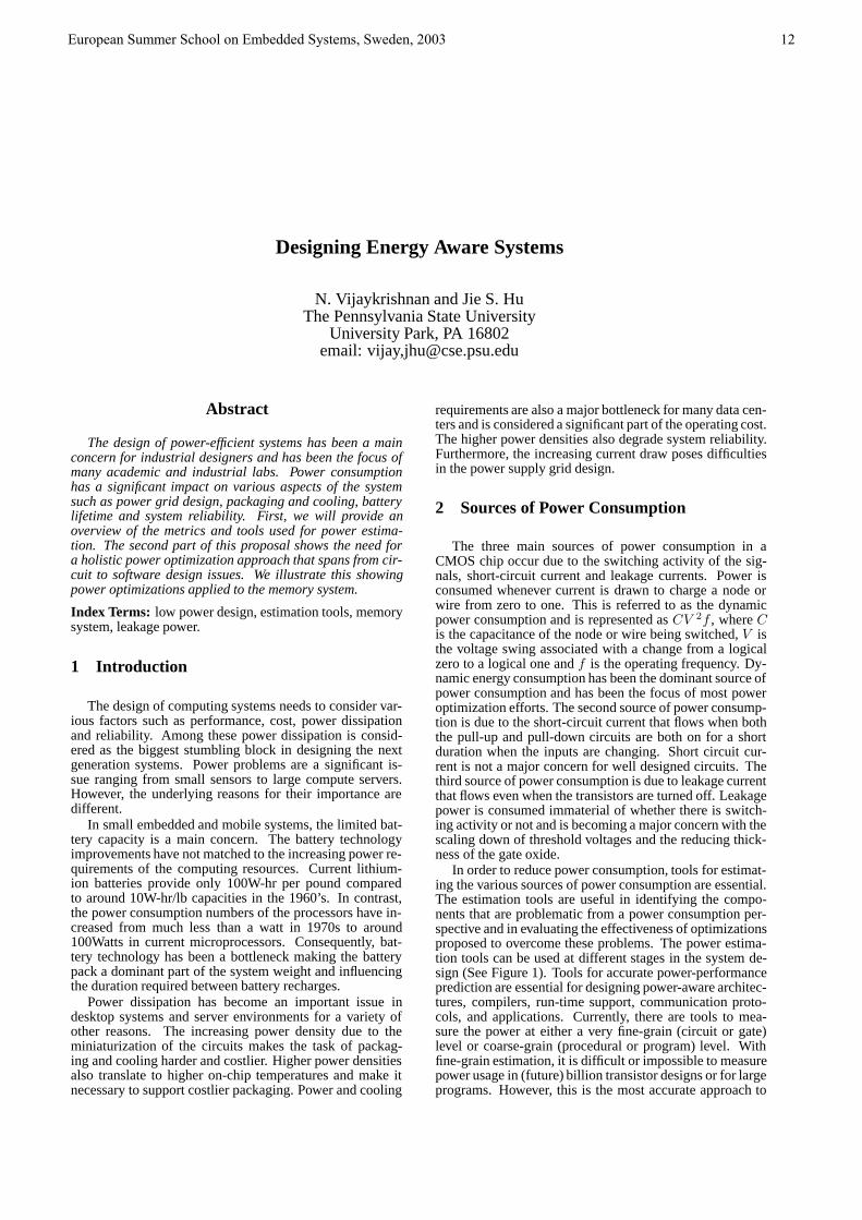
The design of power-efficient systems has been a mainconcern for industrial designers and has been the focus ofmany academic and industrial labs. Power consumptionhas a significant impact on various aspects of the systemsuch as power grid design, packaging and cooling, batterylifetime and system reliability. First, we will provide anoverview of the metrics and tools used for power estima-tion. The second part of this proposal shows the need fora holistic power optimization approach that spans from cir-cuit to software design issues. We illustrate this showingpower optimizations applied to the memory system.
Index Terms: low power design, estimation tools, memorysystem, leakage power.
1 Introduction
The design of computing systems needs to consider var-ious factors such as performance, cost, power dissipationand reliability. Among these power dissipation is consid-ered as the biggest stumbling block in designing the nextgeneration systems. Power problems are a significant is-sue ranging from small sensors to large compute servers.However, the underlying reasons for their importance aredifferent.
In small embedded and mobile systems, the limited bat-tery capacity is a main concern. The battery technologyimprovements have not matched to the increasing power re-quirements of the computing resources. Current lithium-ion batteries provide only 100W-hr per pound comparedto around 10W-hr/lb capacities in the 1960’s. In contrast,the power consumption numbers of the processors have in-creased from much less than a watt in 1970s to around100Watts in current microprocessors. Consequently, bat-tery technology has been a bottleneck making the batterypack a dominant part of the system weight and influencingthe duration required between battery recharges.
Power dissipation has become an important issue indesktop systems and server environments for a variety ofother reasons. The increasing power density due to theminiaturization of the circuits makes the task of packag-ing and cooling harder and costlier. Higher power densitiesalso translate to higher on-chip temperatures and make itnecessary to support costlier packaging. Power and cooling
requirements are also a major bottleneck for many data cen-ters and is considered a significant part of the operating cost.The higher power densities also degrade system reliability.Furthermore, the increasing current draw poses difficultiesin the power supply grid design.
2 Sources of Power Consumption
The three main sources of power consumption in aCMOS chip occur due to the switching activity of the sig-nals, short-circuit current and leakage currents. Power isconsumed whenever current is drawn to charge a node orwire from zero to one. This is referred to as the dynamicpower consumption and is represented as CV 2f , where Cis the capacitance of the node or wire being switched, V isthe voltage swing associated with a change from a logicalzero to a logical one and f is the operating frequency. Dy-namic energy consumption has been the dominant source ofpower consumption and has been the focus of most poweroptimization efforts. The second source of power consump-tion is due to the short-circuit current that flows when boththe pull-up and pull-down circuits are both on for a shortduration when the inputs are changing. Short circuit cur-rent is not a major concern for well designed circuits. Thethird source of power consumption is due to leakage currentthat flows even when the transistors are turned off. Leakagepower is consumed immaterial of whether there is switch-ing activity or not and is becoming a major concern with thescaling down of threshold voltages and the reducing thick-ness of the gate oxide.
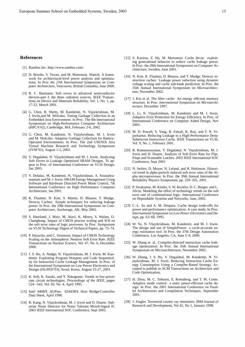
In order to reduce power consumption, tools for estimat-ing the various sources of power consumption are essential.The estimation tools are useful in identifying the compo-nents that are problematic from a power consumption per-spective and in evaluating the effectiveness of optimizationsproposed to overcome these problems. The power estima-tion tools can be used at different stages in the system de-sign (See Figure 1). Tools for accurate power-performanceprediction are essential for designing power-aware architec-tures, compilers, run-time support, communication proto-cols, and applications. Currently, there are tools to mea-sure the power at either a very fine-grain (circuit or gate)level or coarse-grain (procedural or program) level. Withfine-grain estimation, it is difficult or impossible to measurepower usage in (future) billion transistor designs or for largeprograms. However, this is the most accurate approach to
European Summer School on Embedded Systems, Sweden, 2003 12

power estimation. On the other hand, coarse-grain mea-surements can only give gross estimates, but do so quiteefficiently.
At the earliest stage of the design, power is estimated fora given system with little implementation detail at the ar-chitectural level. Architectural power simulators have beentypically built on top of performance simulators that keeptrack of accesses to the different components in the archi-tecture and obtain the power consumption by modeling theper access energy cost of a single access for each compo-nent. The models for the different components are built us-ing the structure, bitwidth and design style. For example,the power consumed for a cache access can be modeled us-ing information such as the size of the cache, the numberof ports and the use of single-ended or double-ended senseamplifiers for reading the data. Examples of architecturallevel estimation tools include Simplepower [24], Softwatt,Wattch [2] and Wattwatcher.
Once the RTL and the corresponding gate level imple-mentation of the architecture are available more accuratepower estimation is possible. Even at this level actual lay-out or circuit implementation is not available and gate andwiring capacitances are estimated using models. Gate ca-pacitances are modeled using the sizing information whilewire loads are obtained from number of pins incident on thenet and based on placement information. The switching ac-tivity at the nodes is estimated through simulation. Oncecapacitance and switching information is available the dy-namic power estimation can be performed.
Later in the design cycle, even more accurate estimatescan be obtained at the circuit level as more information isavailable to make estimates of the capacitance more accu-rately. However, estimation at the higher levels is becomingmore and more important as power problems identified laterin the design cycle are hard to fix. Consequently, tools forestimating the power at the earliest stage of design are be-coming popular. Since software is becoming an integral partof most systems, tools for estimating the power consumedby software and the influence of software optimizations onthe power consumption behavior have also become impor-tant.
These tools also help to identify the specific compo-nents that pose the main concern from a power consump-tion perspective. In many embedded systems, the designof the memory system is a critical factor influencing thepower consumption profile. The rest of this paper showshow memory power optimizations can be reduced at differ-ent levels of system design.
3 Memory Power Optimizations
A host of hardware optimizations have been proposed toreduce the energy consumption. Focusing on SRAM mem-ories, common techniques used for optimization includepartitioning the memory into smaller parts, dividing the bitlines, dividing the word lines and using reduced voltageswings [12]. Two common optimizations applied to cachememories are block buffering [17] and cache subbanking[23]. In the block buffering scheme, the previously accessedcache line is buffered for subsequent accesses [17]. If the
Best Slowest Most
Worst Fastest Least
AccuracyAnalysis
SpeedAnalysis
ResourcesAnalysis
Least
Most
EnergySavings
Abstraction Level
Software
Architectural
Logic (Gate-level)
Transistor (Switch-level)
Figure 1. Comparison of Energy Optimiza-tions at Different Levels.
data within the same cache line is accessed on the next datarequest, only the buffer needs to be accessed. This avoidsthe unnecessary and more energy consuming access to theentire cache data and tag array. Multiple block buffers canbe thought of as a small sized Level 0 cache. In the cachesubbanking optimization, which is also known as columnmultiplexing [23], the data array of the cache is divided intoseveral subbanks and only the subbank where the desireddata is located is accessed. This optimization reduces theper access energy consumption.
A common power optimization technique employed inDRAM memories include the support for multiple lowpower modes. Each mode is characterized by its power con-sumption and the time that it takes to transition back to theactive mode (resynchronization time). Typically, lower theenergy consumption, higher the resynchronization time [1].These modes are characterized by varying degrees of themodule components being active. The power mode tran-sitions can be effected either by hardware or through soft-ware.
In the hardware approach, there is a Self-Monitoring andPrediction Hardware block which monitors ongoing mem-ory transactions. It contains some prediction hardware toestimate the time until the next access to a memory bankand circuitry to ask the memory controller to initiate modetransitions. Limited amount of such self-monitored power-down is present in current memory controllers (e.g., Intel82443BX [13]). The specific details of different predictionmechanisms that can be employed is given in [7]
In the software-directed approach, the memory con-troller is explicitly told to issue the control packets for aspecific module’s mode transitions. A set of configurationregisters in the memory controller that are mapped into theaddress space of the CPU (similar to the registers in thememory controller in [13]) are used to set the power mode.Programming these registers using one or more CPU in-structions (stores) would result in the desired power modesetting. The power modes are set based on analyzing thecode and data access patterns using the compiler.
In addition, it is also possible to use code optimizationsto improve the effectiveness of the power mode control. Forexample, all data accessed can be clustered together in asingle module instead of being scattered across in differentmodules. This enables to put the unused modules into alower power mode.
European Summer School on Embedded Systems, Sweden, 2003 13
4 Reducing Leakage Energy
There have been several efforts spanning from the circuitlevel to the architectural level at reducing the cache leakageenergy. Circuit mechanisms include adaptive substrate bi-asing, dynamic supply scaling and supply gating. Many ofthe circuit techniques have been exploited at the architec-tural level to control leakage at the cache bank and cacheline granularities.
The approaches that target reducing cache leakage en-ergy consumption can be broadly categorized into threegroups: (i) those that base their leakage management de-cisions on some form of performance feedback (e.g., cachemiss rate) [19], (ii) those that manage cache leakage in anapplication insensitive manner (e.g., periodically turning offcache lines) [8, 15, 16], and (iii) those that use feedbackfrom the program behavior [15, 27, 25, 11].
The approach such as DRI I-Cache [19] in category (i)is inherently coarse-grain in managing leakage as it turnsoff large portions of the cache depending on a performancefeedback that does not specifically capture cache line usagepatterns.
Approaches in category (ii) turn off cache lines inde-pendent of the instruction access pattern. An example ofsuch a scheme is the periodic cache line turn-off proposedin [8]. The success of this strategy depends on how wellthe selected period reflects the rate at which the instruc-tion working set changes. Specifically, the optimum periodmay change not only across applications but also within thedifferent phases of the application itself. A second exam-ple of a fixed scheme in category (ii) is the technique pro-posed in [16]. This technique adopts a bank based strategy,where when execution moves from one bank to another, thehardware turns off the former and turns on the latter. An-other technique in category (ii) is the cache decay-based ap-proach (its adaptive variant falls in category (iii)) proposedby Kaxiras et al [15]. In this technique, a small counteris attached to each cache line which tracks its access fre-quency. If a cache line is not accessed for a certain numberof cycles, it is placed into the leakage saving mode. Whilethis technique tries to capture the usage frequency of cachelines, it does not directly predict the cache line access pat-tern. Consequently, a cache line whose counter saturates isturned off even if it is going to be accessed in the next cy-cle. Since it is also a periodic approach, choosing a suitabledecay interval is crucial if it is to be successful.
The approaches in category (iii) attempt to manage cachelines in an application-sensitive manner. The adaptive ver-sion of the cache-decay scheme [15] tailors the decay inter-val for the cache lines based on cache line access patterns.They start out with the smallest decay interval for eachcache line to aggressively turn off cache lines and increasethe decay interval when they learn that the cache lines wereturned off prematurely. These schemes learn about prema-ture turn-off by leaving the tags on at all times. The ap-proach in [27] also uses tag information to adapt leakagemanagement. In [25], an optimizing compiler is used toanalyze the program to insert explicit cache line turn-offinstructions. This scheme demands sophisticated programanalysis and modification support, and needs modificationsin the ISA to implement cache line turn-on/off instructions.
Further, Hu et al., in [11], proposed a hotspot based leakagemanagement scheme to capture the dynamic phase execu-tion information of the running program for directing leak-age control and a just-in-time activation scheme to signifi-cantly reduce the performance overhead due to the leakagecontrol.
As Java technologies are more widely adopted in bat-tery powered devices such as cellphones, PDAs, and pagers,optimizing the power consumption in Java environment isbecoming a critical issue. Java virtual machine (JVM) re-lies on the garbage collector (GC) for automatic memorymanagement. In [4], Chen et al. proposed a GC-controlledleakage energy optimization technique that shuts off mem-ory banks that do not hold live data. Their schemes reducethe leakage energy consumed by the heap memory signifi-cantly. However, conventional GC is invoked at a fixed fre-quency to detect and turn off the memory banks containingno live objects. High frequent GC will unnecessarily de-crease the performance of the virtual machine. On the otherside, GC at very low frequency will lose the opportunitiesfor leakage optimization. The optimal GC frequency de-pends on the behavior of a particular application. In [5], theauthors further developed an adaptive scheme that dynami-cally adjusts the GC frequency according to the memory al-location behavior of the applications. This adaptive schemeprovides a leakage reduction approaching that delivered bythe optimal GC frequency of a given application.
In attempting to reduce leakage energy, we might in-crease the susceptibility to soft errors when reducing sup-ply voltages. The work [26] provides a detailed investiga-tion on impacts of soft errors in caches applying drowsyleakage control scheme. The results indicate that the singleevent upset rate (SER) increases dramatically from 2.5E-05 FIT/bit to 5E05 FIT/bit when the supply voltage is re-duced from the normal voltage 1.0V to a drowsy voltage0.3V. Hence to maintain the system reliability, more sophis-ticated error protection schemes that themselves will con-sume more energy will be required. Hence, as these re-liability problems aggravate, devising techniques that willbalance the tradeoffs between energy optimization and reli-ability will become important.
5 Conclusions
Power consumption has become a major design con-straint influencing the design of next generation systems.Combating the power problem requires a holistic effortspanning from circuits to software. Furthermore, there isa complex interaction and tradeoff between power, perfor-mance and reliability that need to be balanced carefully.
Acknowledgment
This work was supported in part by grants from NSFCAREER Award 0093085, and Gigascale Silicon ResearchCenter. The author would like to acknowledge Profs. MaryJane Irwin and Mahmut Kandemir and students in the Mi-crosystems Design Lab who were involved in parts of theseprojects reported here.
European Summer School on Embedded Systems, Sweden, 2003 14
References
[1] Rambus Inc. http://www.rambus.com/.
[2] D. Brooks, V. Tiwari, and M. Martonosi. Wattch: A frame-work for architectural-level power analysis and optimiza-tions. In Proc the 27th International Symposium on Com-puter Architecture, Vancouver, British Columbia, June 2000.
[3] R. C. Baumann. Soft errors in advanced semiconductordevices-part I: the three radiation sources. IEEE Transac-tions on Device and Materials Reliability, Vol. 1, No. 1, pp.17-22, March 2001.
[4] G. Chen, R. Shetty, M. Kandemir, N. Vijaykrishnan, M.J. Irwin,and M. Wolczko. Tuning Garbage Collection in anEmbedded Java Environment. In Proc. The 8th InternationalSymposium on High-Performance Computer Architecture(HPCA’02), Cambridge, MA, February 2-6, 2002.
[5] G. Chen, M. Kandemir, N. Vijaykrishnan, M. J. Irwinand M. Wolczko. Adaptive Garbage Collection for Battery-Operated Environments. In Proc. The 2nd USENIX JavaVirtual Machine Research and Technology Symposium(JVM’02), August 1-2, 2002.
[6] V. Degalahal, N. Vijaykrishnan and M. J. Irwin. AnalyzingSoft Errors in Leakage Optimized SRAM Designs. To ap-pear in Proc. of International Conference on VLSI Design,Jan 2003.
[7] V. Delaluz, M. Kandemir, N, Vijaykrishnan, A. Sivasubra-maniam and M. J. Irwin. DRAM Energy Management UsingSoftware and Hardware Directed Power Mode Control, 7thInternational Conference on High Performance ComputerArchitecture, Jan 2001.
[8] K. Flautner, N. Kim, S. Martin, D. Blaauw, T. Mudge.Drowsy Caches: Simple techniques for reducing leakagepower. In Proc. the 29th International Symposium on Com-puter Architecture, Anchorage, AK, May 2002.
[9] S. Hareland, J. Maiz, M. Alavi, K. Mistry, S. Walsta, D.Changhong. Impact of CMOS process scaling and SOI onthe soft error rates of logic processes. In Proc. Symposiumon VLSI Technology Digest of Technical Papers. pp. 73–74.
[10] P. Hazucha, and C. Svensson, Impact of CMOS TechnologyScaling on the Atmospheric Neutron Soft Error Rate. IEEETransactions on Nuclear Science, Vol. 47, No. 6, December2000.
[11] J. S. Hu, A. Nadgir, N. Vijaykrishnan, M. J. Irwin, M. Kan-demir. Exploiting Program Hotspots and Code Sequential-ity for Instruction Cache Leakage Management. In Proc. ofthe International Symposium on Low Power Electronics andDesign (ISLPED’03), Seoul, Korea, August 25-27, 2003.
[12] K. Itoh, K. Sasaki, and Y. Nakagome. Trends in low-powerram circuit technologies. Proceedings of the IEEE, pages524 –543, Vol. 83. No. 4, April 1995.
[13] Intel 440BX AGPset: 82443BX Host Bridge/ControllerData Sheet, April 1998.
[14] B. Kang, N. Vijaykrishnan, M. J. Irwin and D. Duarte. Sub-strate Noise Detector for Noise Tolerant Mixed-Signal IC2003 IEEE International SOC Conference, Sept 2003.
[15] S. Kaxiras, Z. Hu, M. Martonosi. Cache decay: exploit-ing generational behavior to reduce cache leakage power.In Proc. the 28th International Symposium on Computer Ar-chitecture, Sweden, June 2001.
[16] N. Kim, K. Flautner, D. Blaauw, and T. Mudge. Drowsy in-struction caches: Leakage power reduction using dynamicvoltage scaling and cache sub-bank prediction. In Proc. the35th Annual International Symposium on Microarchitec-ture, November 2002.
[17] J. Kin et al. The filter cache: An energy efficient memorystructure. In Proc. International Symposium on Microarchi-tecture, December 1997.
[18] L. Li, N. Vijaykrishnan, M. Kandemir and M. J. Irwin.Adaptive Error Protection for Energy Efficiency. In Proc. ofInternational Conference on Computer Aided Design, Nov2003.
[19] M. D. Powell, S. Yang, B. Falsafi, K. Roy, and T. N. Vi-jaykumar. Reducing Leakage in a High-Performance Deep-Submicron Instruction Cache. IEEE Transactions on VLSI,Vol. 9, No. 1, February 2001.
[20] R. Ramanarayanan, V. Degalahal, N. Vijaykrishnan, M. J.Irwin and D. Duarte. Analysis of Soft-Error Rate for Flip-Flops and Scannable Latches. 2003 IEEE International SOCConference, Sept 2003
[21] N. Seifert, D. Moyer, N. Leland, and R. Hokinson. Histori-cal trend in alpha-particle induced soft error rates of the Al-pha microprocessor. In Proc. the 39th Annual InternationalReliability Physics Symposium, pp. 259–265, 2001.
[22] P. Sivakumar, M. Kistler, S. W. Keckler, D. C. Burger, and L.Alvisi. Modeling the effect of technology trends on the softerror rate of combinational logic. International Conferenceon Dependable Systems and Networks, June, 2002.
[23] C.-L. Su and A. M. Despain. Cache design trade-offs forpower and performance optimization: A case study, In Proc.International Symposium on Low Power Electronics and De-sign, pp. 63–68, 1995.
[24] W. Ye, N. Vijaykrishnan, M. Kandemir, and M. J. Irwin.The design and use of SimplePower: a cycle-accurate en-ergy estimation tool. In Proc. the 37th Design AutomationConference, Los Angeles, CA, June 5–9, 2000.
[25] W. Zhang et. al.. Compiler-directed instruction cache leak-age optimization. In Proc. the 35th Annual InternationalSymposium on Microarchitecture, November 2002.
[26] W. Zhang, J. S. Hu, V. Degalahal, M. Kandemir, N. Vi-jaykrishnan, M. J. Irwin. Reducing Instruction Cache En-ergy Consumption Using a Compiler-Based Strategy. Ac-cepted to publish in ACM Transactions on Architecture andCode Optimization.
[27] H. Zhou, M. C. Toburen, E. Rotenberg, and T. M. Conte.Adaptive mode control: a static power-efficient cache de-sign. In Proc. the 2001 International Conference on Paral-lel Architectures and Compilation Techniques, September2001.
[28] J. Ziegler. Terrestrial cosmic ray intensities. IBM Journal ofResearch and Development, Vol 42, No 1, January 1998.
European Summer School on Embedded Systems, Sweden, 2003 15
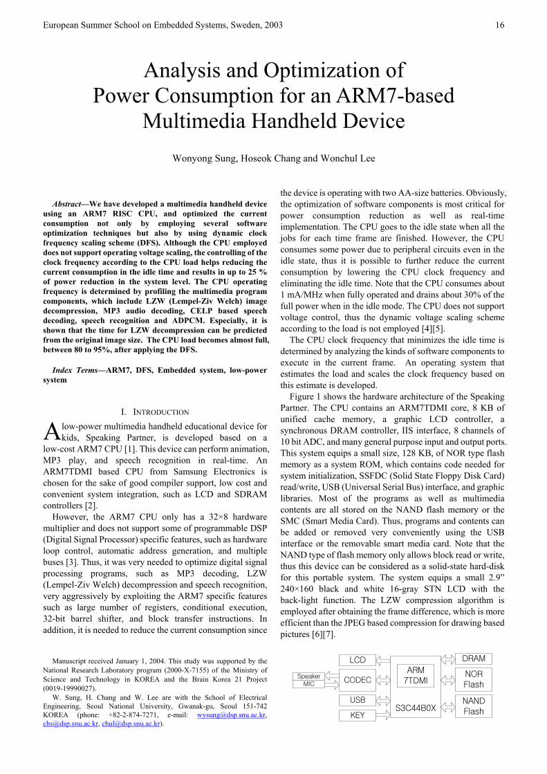
European Summer School on Embedded Systems, Sweden, 2003
16
Analysis and Optimization of Power Consumption for an ARM7-based
Multimedia Handheld Device Wonyong Sung, Hoseok Chang and Wonchul Lee
Abstract—We have developed a multimedia handheld device
using an ARM7 RISC CPU, and optimized the current consumption not only by employing several software optimization techniques but also by using dynamic clock frequency scaling scheme (DFS). Although the CPU employed does not support operating voltage scaling, the controlling of the clock frequency according to the CPU load helps reducing the current consumption in the idle time and results in up to 25 % of power reduction in the system level. The CPU operating frequency is determined by profiling the multimedia program components, which include LZW (Lempel-Ziv Welch) image decompression, MP3 audio decoding, CELP based speech decoding, speech recognition and ADPCM. Especially, it is shown that the time for LZW decompression can be predicted from the original image size. The CPU load becomes almost full, between 80 to 95%, after applying the DFS.
Index Terms—ARM7, DFS, Embedded system, low-power system
I. INTRODUCTION
Alow-power multimedia handheld educational device for kids, Speaking Partner, is developed based on a
low-cost ARM7 CPU [1]. This device can perform animation, MP3 play, and speech recognition in real-time. An ARM7TDMI based CPU from Samsung Electronics is chosen for the sake of good compiler support, low cost and convenient system integration, such as LCD and SDRAM controllers [2].
However, the ARM7 CPU only has a 32×8 hardware multiplier and does not support some of programmable DSP (Digital Signal Processor) specific features, such as hardware loop control, automatic address generation, and multiple buses [3]. Thus, it was very needed to optimize digital signal processing programs, such as MP3 decoding, LZW (Lempel-Ziv Welch) decompression and speech recognition, very aggressively by exploiting the ARM7 specific features such as large number of registers, conditional execution, 32-bit barrel shifter, and block transfer instructions. In addition, it is needed to reduce the current consumption since
the device is operating with two AA-size batteries. Obviously, the optimization of software components is most critical for power consumption reduction as well as real-time implementation. The CPU goes to the idle state when all the jobs for each time frame are finished. However, the CPU consumes some power due to peripheral circuits even in the idle state, thus it is possible to further reduce the current consumption by lowering the CPU clock frequency and eliminating the idle time. Note that the CPU consumes about 1 mA/MHz when fully operated and drains about 30% of the full power when in the idle mode. The CPU does not support voltage control, thus the dynamic voltage scaling scheme according to the load is not employed [4][5].
Manuscript received January 1, 2004. This study was supported by the
National Research Laboratory program (2000-X-7155) of the Ministry of Science and Technology in KOREA and the Brain Korea 21 Project (0019-19990027).
W. Sung, H. Chang and W. Lee are with the School of Electrical Engineering, Seoul National University, Gwanak-gu, Seoul 151-742 KOREA (phone: +82-2-874-7271, e-mail: [email protected], [email protected], [email protected]).
The CPU clock frequency that minimizes the idle time is determined by analyzing the kinds of software components to execute in the current frame. An operating system that estimates the load and scales the clock frequency based on this estimate is developed.
Figure 1 shows the hardware architecture of the Speaking Partner. The CPU contains an ARM7TDMI core, 8 KB of unified cache memory, a graphic LCD controller, a synchronous DRAM controller, IIS interface, 8 channels of 10 bit ADC, and many general purpose input and output ports. This system equips a small size, 128 KB, of NOR type flash memory as a system ROM, which contains code needed for system initialization, SSFDC (Solid State Floppy Disk Card) read/write, USB (Universal Serial Bus) interface, and graphic libraries. Most of the programs as well as multimedia contents are all stored on the NAND flash memory or the SMC (Smart Media Card). Thus, programs and contents can be added or removed very conveniently using the USB interface or the removable smart media card. Note that the NAND type of flash memory only allows block read or write, thus this device can be considered as a solid-state hard-disk for this portable system. The system equips a small 2.9” 240×160 black and white 16-gray STN LCD with the back-light function. The LZW compression algorithm is employed after obtaining the frame difference, which is more efficient than the JPEG based compression for drawing based pictures [6][7].
S3C44B0X
ARM7TDMI
DRAM
NORFlash
NANDFlash
LCD
CODEC
USB
SpeakerMIC
KEY

European Summer School on Embedded Systems, Sweden, 2003
17
Fig. 1. System architecture.
II. MUILTI-TASKING OPERATING SYSTEM AND DYNAMIC FREQEUNCY SCALING
Since the system should conduct several multimedia functions simultaneously, a simple real-time operating system is developed. Figure 2 shows the time-assignment for 6 tasks where the audio input and output tasks are processed as top priority jobs. Note that audio jobs can cause more serious damage than graphic functions when a job for this frame is postponed to the next frame due to the shortage of CPU clock cycles.
480msec240msec time
Frame length
Idle task
Graphic output
System control
Audio input
Audio output
Animation player
Block
Run
Idle
Fig. 2. The time-assignment for real-time operation.
The frame length, which can be changed by software, is
normally set to 240 msec due to the low response time of the STN LCD. As shown in Fig. 2, the CPU goes to the idle state when all the jobs for the current frame are finished.
Figure 3 shows the current consumption of the CPU according to the load condition when the CPU clock frequency is 60 MHz, 30 MHz and dynamically changed. The current measured indicates all the currents needed for this system, except for speaker drive and back light, when the system is conducting LZW compression. The CPU load is controlled by changing the size and the number of images to decompress. As shown in this figure, the CPU drains some power even when the CPU load is very small although the CPU is mostly in the idle state. Thus, it is advantageous for power reduction to employ the lowest possible clock frequency. Obviously, the estimation of the minimum clock frequency for a real-time implementation is needed.
The current consumption for the CPU load of 20% is 120 mA when the clock speed is 60 MHz without any idle state transition. According to Fig. 3, 95 mA is consumed when the clock speed is 60MHz with idle state, and 72 mA when the dynamic frequency scaling is employed. This shows that the dynamic frequency scaling scheme is more efficient than the constant frequency operation with idle state when the load condition is low.
60
70
80
90
100
110
120
130
140
150
0 20 40 60 80 100
CPU Load(%)
Curr
ent(m
A)
60MHz
30MHz
DFS
Fig. 3. Current consumption of constant frequency system with idle state and dynamic frequency system.
Table 1 shows the current consumption at each hardware block when the CPU load is 10%. As shown in this table, the current consumption in the CPU is more drastically reduced, more than 67%, although the total system current is reduced by 26%.
TABLE 1.
CURRENT CONSUMPTION AT EACH HARDWARE BLOCK. Current Hardware blockConstant freq. DFS
CPU 34 mA 11 mA (-67%) DRAM 29 mA 29 mA LCD display 15 mA 15 mA Others 11 mA 11 mA Total 89 mA 66 mA (-26%)
III. SOFTWARE OPTIMIZATION TECHNIQUES The ARM7TDMI processor has a relatively simple data
path, where the hardware multiplier only has the accuracy of 32×8 bits. This may mean that the CPU is not good for executing multiplication intensive digital signal processing programs. However, the CPU has a few advantageous characteristics for implementing DSP algorithms [8][9]. Firstly, it has a fairy large number of registers, 31 for general purpose, when compared with traditional programmable digital signal processors. Thus, it helps much for reducing the memory accesses and shows a quite good compiler performance. Secondly, most of the instructions can be executed conditionally. It significantly reduces the control overhead in control intensive routines like the Huffman decoder. Thirdly, it has a 32-bit barrel shifter that can simultaneously execute shift and rotation with ALU operations. This feature is useful for scaling and multiplication by 2 constant. Fourthly, block load and store (LDM, STM) instructions are supported, which move 16 registers from or to memory using a single instruction. Note that the block load and store instructions are not normally found at the inside of functions in the compiler generated codes, thus it needs some manual assembly coding to utilize these instructions.
Figure 4 shows the implementation results, in terms of the
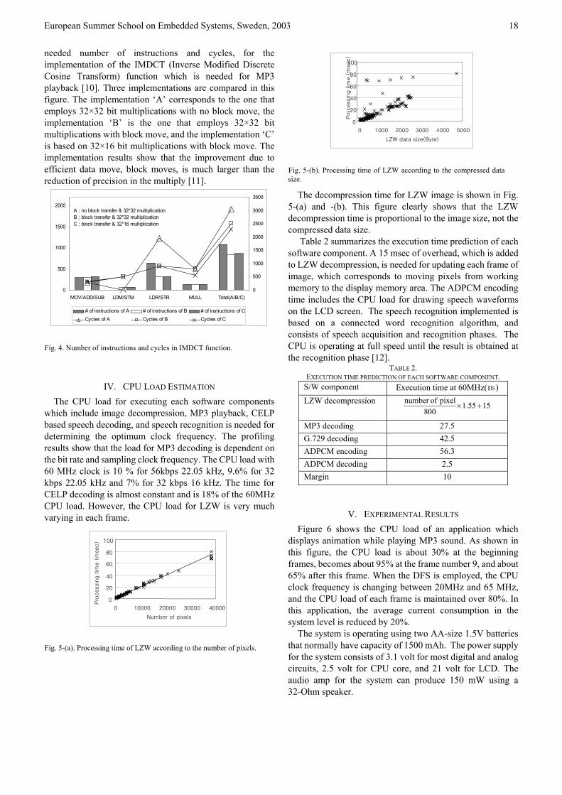
European Summer School on Embedded Systems, Sweden, 2003
18
needed number of instructions and cycles, for the implementation of the IMDCT (Inverse Modified Discrete Cosine Transform) function which is needed for MP3 playback [10]. Three implementations are compared in this figure. The implementation ‘A’ corresponds to the one that employs 32×32 bit multiplications with no block move, the implementation ‘B’ is the one that employs 32×32 bit multiplications with block move, and the implementation ‘C’ is based on 32×16 bit multiplications with block move. The implementation results show that the improvement due to efficient data move, block moves, is much larger than the reduction of precision in the multiply [11].
0
500
1000
1500
2000
MOV/ADD/SUB LDM/STM LDR/STR MULL Total(A/B/C)0
500
1000
1500
2000
2500
3000
3500
# of instructions of A # of instructions of B # of instructions of CCycles of A Cycles of B Cycles of C
A : no block transfer & 32*32 multiplicationB : block transfer & 32*32 multiplicationC : block transfer & 32*16 multiplication
Fig. 4. Number of instructions and cycles in IMDCT function.
IV. CPU LOAD ESTIMATION The CPU load for executing each software components
which include image decompression, MP3 playback, CELP based speech decoding, and speech recognition is needed for determining the optimum clock frequency. The profiling results show that the load for MP3 decoding is dependent on the bit rate and sampling clock frequency. The CPU load with 60 MHz clock is 10 % for 56kbps 22.05 kHz, 9.6% for 32 kbps 22.05 kHz and 7% for 32 kbps 16 kHz. The time for CELP decoding is almost constant and is 18% of the 60MHz CPU load. However, the CPU load for LZW is very much varying in each frame.
0 20
40
60
80
100
0 10000 20000 30000 40000
Number of pixels
Pro
cessin
g tim
e (
msec)
Fig. 5-(a). Processing time of LZW according to the number of pixels.
0
20
40
60
80
100
0 1000 2000 3000 4000 5000
LZW data size(Byte)
Pro
cessin
g tim
e (
msec)
Fig. 5-(b). Processing time of LZW according to the compressed data size.
The decompression time for LZW image is shown in Fig. 5-(a) and -(b). This figure clearly shows that the LZW decompression time is proportional to the image size, not the compressed data size.
Table 2 summarizes the execution time prediction of each software component. A 15 msec of overhead, which is added to LZW decompression, is needed for updating each frame of image, which corresponds to moving pixels from working memory to the display memory area. The ADPCM encoding time includes the CPU load for drawing speech waveforms on the LCD screen. The speech recognition implemented is based on a connected word recognition algorithm, and consists of speech acquisition and recognition phases. The CPU is operating at full speed until the result is obtained at the recognition phase [12].
TABLE 2. EXECUTION TIME PREDICTION OF EACH SOFTWARE COMPONENT.
S/W component Execution time at 60MHz() LZW decompression 1555.1
800pixel ofnumber
+×
MP3 decoding 27.5 G.729 decoding 42.5 ADPCM encoding 56.3 ADPCM decoding 2.5 Margin 10
V. EXPERIMENTAL RESULTS Figure 6 shows the CPU load of an application which
displays animation while playing MP3 sound. As shown in this figure, the CPU load is about 30% at the beginning frames, becomes about 95% at the frame number 9, and about 65% after this frame. When the DFS is employed, the CPU clock frequency is changing between 20MHz and 65 MHz, and the CPU load of each frame is maintained over 80%. In this application, the average current consumption in the system level is reduced by 20%.
The system is operating using two AA-size 1.5V batteries that normally have capacity of 1500 mAh. The power supply for the system consists of 3.1 volt for most digital and analog circuits, 2.5 volt for CPU core, and 21 volt for LCD. The audio amp for the system can produce 150 mW using a 32-Ohm speaker.

European Summer School on Embedded Systems, Sweden, 2003
19
0
20
40
60
80
100
1 2 3 4 5 6 7 8 9 10 11 12 13 14 15
frame(240msec per frame)
CP
U load(%
)
15
25
35
45
55
65
Fre
q.(
MH
z)
Constant freq. Dynamic freq. Clock freq.
Figure 6. CPU load of constant and dynamic frequency systems.
The current consumption measured at 3.0 volt supply (battery terminals) is shown in Table 3 according to the activity of the system. Note that the power for speaker driving is included.
TABLE 3.
CURRENT CONSUMPTION ACCORDING TO EACH ACTIVITY. Activity CPU load Original
current Optimized current
Menu display 11 % 92 mA 68 mA Song with animation 65 % 175 mA 160 mA Speech recognition 100 % 150 mA 150 mA MP3 play 10 % 125 mA 100 mA
VI. CONCLUDING REMARKS A low-power handheld multimedia device is developed
using an ARM7 CPU. A dynamic frequency scaling scheme is employed in order to reduce the CPU power consumption, which shows that about 20 % of system power saving can be achieved when compared to constant frequency operating scheme with idle state. The CPU clock frequency is determined by the real-time operating system, which sums up the CPU loads needed for executing all the software components. The amount of clock cycles for implementing each software component is measured by profiling. Obviously, the current can be further reduced, without any significant change in the power reduction algorithm, if we employ a CPU that supports the dynamic voltage scaling, such as Intel’s Xscale [13].
REFERENCES [1] http://www.edumtek.com. [2] S3C44B0X RISC Microprocessor User’s Manual, Samsung
Electronics, 2001. [3] ARM Architecture Reference Manual, ARM, 1996. [4] Tajana Simunic, Luca Benini and Giovanni De Micheli,
"Energy-Efficient Design of Battery-Powered Embedded Systems," IEEE Trans. on VLSI. Systems, vol. 9, no. 1, Feb. 2001.
[5] Y.Li and J.Henkel, "A Framework for Estimating and Minimizing Energy Dissipation of Embedded HW/SW Systems," IEEE Proc. Design Automation Conf., 1998, pp. 188-193.
[6] T. A. Welch, “A Technique for High-Performance Data Compression,” IEEE Computer, 8-19, June 1984.
[7] G.K. Wallace, “The JPEG Still Picture Compression Standard,” Communications of the ACM, 34(4):30-44, 1991.
[8] Ki-Il Kum, Jiyang Kang and Wonyong Sung, “Autoscaler for C : An Optimizing Floating-Point to Integer C Program Converter For Fixed-Point Digital Signal Processors,” IEEE Transactions on Circuits and Systems, vol.47, no.9, Sep. 2000.
[9] V.Zivojnovic, “Compilers for Digital Signal Processors,” DSP & Multimedia Technol., vol.4, no.5, pp.27-45, July 1995.
[10] Vladimir Britanak and K.R.Rao, “An Efficient Implementation of the Forward and Inverse MDCT in MPEG Audio Coding,” IEEE Signal Processing Letters, vol.8, no.2, Feb. 2001.
[11] Wonchul Lee, Kisun You and Wonyong Sung, “Software Optimization of MPEG Audio Layer-III For a 32bit RISC Processor,” IEEE Asia Pacific Conference on Circuits And Systems, Oct. 2002.
[12] Suhong Ryu, Younim Lee and Wonyong Sung, "Implementation of Speech Recognition Algorithm for An 32-bit CPU-Based Portable Device," IEEE Conference of Consumer Electronics, June 2002.
[13] Intel XScale Microarchitecture Data Sheet, Intel, 2000. Wonyong Sung (S’84–M’87) received the B.S. degree in electronic engineering from Seoul National University, Seoul, Korea, in 1978, the M.S. degree in electrical engineering from the Korea Advanced Institute of Science and Technology (KAIST), Seoul, Korea, in 1980, and the Ph.D. degree in electrical and computer engineering from the University of California at Santa Barbara in 1987. He has been a Member of the Faculty of the Seoul National University since 1989. From 1980 to 1983, he was with the Central Research Laboratory of Gold Star (currently LG Electronics), Korea. During his Ph.D. studies, he developed parallel processing algorithms, vector and multiprocessor implementation, and low-complexity FIR filter design. From May 1993 to June 1994, he consulted with the Alta Group for the development of the fixed-point optimizer, automatic word-length determination, and scaling software. His current research interests include the development of fixed-point optimization tools, implementation of VLSI for digital signal processing, and multiprocessor-based implementations. Dr. Sung is a technical committee member of the IEEE Signal Processing Society Design and Implementation (DISPS) and that of the IEEE Circuits and Systems VLSI Systems and Application Technical Committee (VSATC). He was the general chair of the IEEE 2003 Signal Processing Systems Workshop held in Seoul, KOREA.

European Summer School on Embedded Systems, Sweden, 2003 20
A Cycle-Accurate Joulemeter for CMOS VLSI Circuits
Eunseok Song, In-Chan Choi, Young-Kil Park and Soo-Ik Chae
School of Electrical Engineering & Inter-university Semiconductor Research Center, Seoul National University
Kwanak P.O. Box 34, Seoul 151-742, KOREA E-mail: [email protected]
Abstract
Cycle-accurate energy measurement is very useful in reducing the energy consumption in the CMOS VLSI circuits, which was reported in [1]. This paper introduces a simple energy measure system, describes three energy models for the CMOS circuits, and derives their energy equations for a clock edge. Then, we compare their accuracy with the simulation and experiment results for a simple inverter. We found that instead of representing all load capacitance as a capacitor to ground, we should separate the capacitance to ground and that to supply for accurate energy analysis in implementing an accurate joulemeter. 1. INTRODUCTION
There have been several methods to estimate the per-cycle energy or power consumed in a CMOS VLSI circuit [2], [3]. Simulator-based energy estimation methods are simple and popular. Low-level energy estimators are accurate but slow for a complex circuit. On the other hand high-level simulators are fast but inaccurate.
We can measure the energy consumed in a CMOS VLSI circuit by integrating the instantaneous current value when the supply voltage is constant. However, what we can measure with an ammeter is not the instantaneous current but its time-average. To overcome this limitation, measurement using capacitors and switches was recently proposed by Chang [1].
The contents of the lecture are as follows:
IntroductionEnergy Estimation in Measurement System• Energy model 1• Energy model 2• Energy model 3• Energy model 4
Second Order Effects• Leakage current• Overlapping current• Nonlinear capacitance
Experimental Results• Altera FPGA• ARM7TDMI
2. ENERGY MEASUREMENT SYSTEM The methods using external capacitors and switches can
integrate high frequency components inherently, as shown in Fig. 1. First, the capacitor CM is charged to a certain reset level before arriving a clock edge. Although the current is spiky when the energy is consumed in the chip, we can
calculate the consumed energy by measuring the voltage drop of VM. The energy transferred into the chip can be written as follows,
22
21 2
121 VCVCE MM −=
VLSIChipVLSIChip
VS
Clock
VM
IM
Clock
VM
IM
V1CM V2
Fig. 1. Energy measurement using a capacitor and a switch.
The energy E is consumed or stored in the chip under measurement. A typical block diagram of the energy measurement system using a capacitor and two switches is shown in Fig. 2.
CM
ADCADCAmpAmp
VSS1 S2VM
CL
Power Line
Test Digital IC
Data AcquisitionController
Data AcquisitionController
Host Computer
ClockGenerator
ClockGenerator
Switch Control
VB
CB
Fig. 2. Cycle-accurate energy measurement system using a capacitor and
two switches. First, switch S1 is closed before arriving a clock edge,
which charges capacitor CM. to the supply voltage level VS. Switch S2 is open during charging capacitor CM, which separates the chip from the supply. Note that capacitor CB models the total capacitance connected to the internal power line, including the on-chip decoupling capacitance, which varies after every clock edge. Note that switch S2 is used to determine the value of capacitor CB. Capacitor CL represents the internal load capacitance, which also varies after every clock edge. An amplifier is employed to amplify the voltage drop of VM to meet the ADC input range of 1 or 2 volts. The voltage drop of VM should be limited not to disturb the proper operation of the chip. Consequently, the voltage drop of VM must be within 100~200mV, which can be controlled by adjusting the size of the capacitor CM. The digital data from the ADC is stored in real time in memory. Later, the host computer calculates the consumed energy using the ADC data.
Fig. 3 shows the timing diagram of the control signals in the measurement system in Fig. 2. When S1 is closed, VM is

European Summer School on Embedded Systems, Sweden, 2003 21
charged as VS. When S2 is closed, charge sharing between CM and CB occurs, which induces a small voltage drop of VM. Then, when a clock edge arrives, the chip draws a relatively large current, which makes another voltage drop of VM. Three sampling points for a clock edge are necessary for estimating the consumed energy. Therefore, the clock frequency should be lowered to ensure enough settling time for both recharging and sampling VM for each clock edge.
t0
TM
Tsettling
Clock
S1
S2
VM
t1 t2 t3 t4 t5 t6 t7 t8 t9 t10
VBSampling
Points
Fig. 3. Timing diagram of cycle-accurate energy measurement system.
3. ENERGY CALCULATION MODELS Per-edge energy measurements will require proper
modeling and analysis of its internal circuit. A per-cycle energy measurement can be obtained by adding two consecutive per-edge energy measurements. In this paper we describe three models and derive an expression of how to calculate the energy consumed for a clock edge for each model.
A. Model 1: Energy consumed in the chip under measurement
It calculates the energy transferred from the capacitors CM and CB into the load capacitor CL. If the sampled values of VM before and after a clock edge are represented as V1 and V2, respectively, then we can calculate the consumed energy,
))((21 2
22
11 VVCCE BM −+=
assuming that the capacitors CM and CB are constant. However, CB can change for every clock edge.
To calculate the consumed energy for the rising edge at t=t4, first capacitor CM is charged to the reset level VS after S1 is closed at t=t1. Then, when S2 is closed at t=t3, charge sharing occurs between CM and CB. From the charge conservation law (CCL),
( ) )()()()()( 44333 tVtCCtVtCtVC MBMBBMM +=+
Assuming that no leakage current exist in the device
under measurement, it is clear that VB(t3)=VB(t1)=VM(t1). Furthermore, CB(t3) = CB(t4) because CB does not change before arriving a clock edge. Therefore,
( ) )()()()()( 44143 tVtCCtVtCtVC MBMMBMM +=+
Because CM is a known constant, capacitor CB can be
written as
MMM
MMB C
tVtVtVtVtC
)()()()()(
14
434 −
−=
Similarly,
MMM
MMB C
tVtVtVtVtC
)()()()()(
58
875 −
−=
Consequently, the consumed energy after a clock edge at t=t3 can be written as
( ) ( ) )()(21)()(
21
52
542
41 tVtCCtVtCCE MBMMBM +−+=
Note that because it includes the measurement distortion
due to the measurement setup, it does not equal to the energy consumed in the chip that is in the real operation setup.
B. Model 2: Energy transferred to the chip
Model 2 calculates the energy transferred into the load capacitor after a clock edge, which does not equal to the energy consumed after the edge. In this model, we first calculate the load capacitance CL per clock edge, which does not include any distortion due to the measurement setup, assuming that the load capacitance CL does not depend on the voltage. Then, we can calculate the energy transferred after the edge as follows,
22 DDLVCE = (1)
VDD in Eq. (1) does not mean the VS in the measurement
setup but the supply voltage used in the real application setup. A half of the transferred energy is consumed as a heat in the MOS transistors and the rest of it is stored in many load capacitors in a complex CMOS VLSI circuit. However, the stored energy of 50% is consumed partially when the logic state of an output, where the energy is stored in its load capacitance, is changed.
CM
C1(n)S2
CB
Switch from high to lowC7(n) / C8(n)4
Switch from low to highC5(n) / C6(n)3
Stay in the high stateC3(n) / C4(n)2
Stay in the low stateC1(n) / C2(n)1
DescriptionSymbolGroup
Switch from high to lowC7(n) / C8(n)4
Switch from low to highC5(n) / C6(n)3
Stay in the high stateC3(n) / C4(n)2
Stay in the low stateC1(n) / C2(n)1
DescriptionSymbolGroup
VS
S1
VM VB
C2(n)
C3(n)
C4(n)
C5(n)
C6(n)
C7(n)
C8(n)
Fig. 4. Circuit modeling and four cases according to the output transition at the nth clock edge.
To find CL, we first calculate CB, which is the same with
CB in model 1. After that, we can write CCL for the rising edge at t=t4,
( ) ( ) )()()()()( 55544 tVtCtCCtVtCC MLBMMBM ++=+ Then, CL(t5) can be written as,
( ) ( ))(
)()()()()(5
55445 tV
tVtCCtVtCCtCM
MBMMBML
+−+= (2)
With Eq. (1) and Eq. (2), we can calculate the energy
transferred to the chip after a clock edge
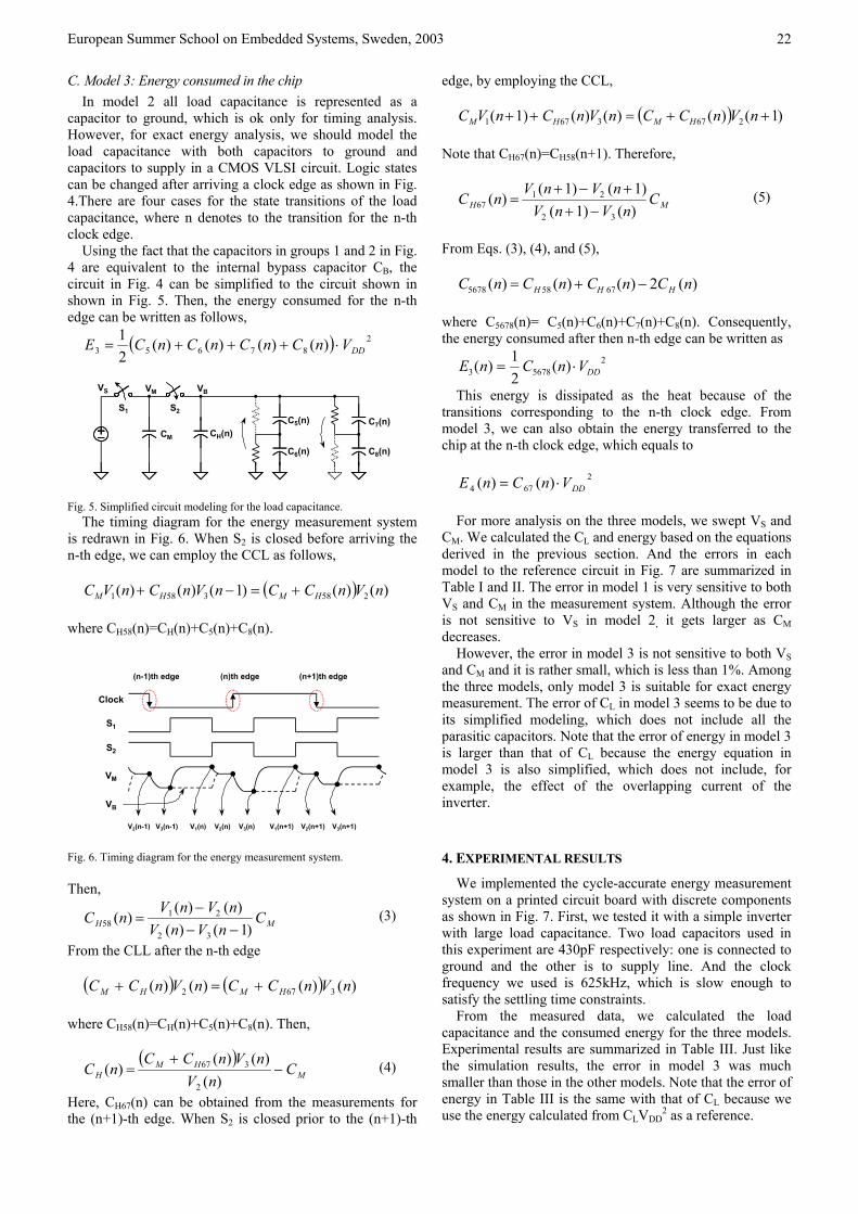
European Summer School on Embedded Systems, Sweden, 2003 22
C. Model 3: Energy consumed in the chip In model 2 all load capacitance is represented as a
capacitor to ground, which is ok only for timing analysis. However, for exact energy analysis, we should model the load capacitance with both capacitors to ground and capacitors to supply in a CMOS VLSI circuit. Logic states can be changed after arriving a clock edge as shown in Fig. 4.There are four cases for the state transitions of the load capacitance, where n denotes to the transition for the n-th clock edge.
Using the fact that the capacitors in groups 1 and 2 in Fig. 4 are equivalent to the internal bypass capacitor CB, the circuit in Fig. 4 can be simplified to the circuit shown in shown in Fig. 5. Then, the energy consumed for the n-th edge can be written as follows,
( 287653 )()()()(
21
DDVnCnCnCnCE ⋅+++= )
CM
C6(n)
C5(n)
C8(n)
C7(n)CH(n)
VS
S1 S2
VM VB
Fig. 5. Simplified circuit modeling for the load capacitance. The timing diagram for the energy measurement system
is redrawn in Fig. 6. When S2 is closed before arriving the n-th edge, we can employ the CCL as follows,
( ) )()()1()()( 2583581 nVnCCnVnCnVC HMHM +=−+
where CH58(n)=CH(n)+C5(n)+C8(n).
(n-1)th edge
Clock
S1
S2
VM
VB
(n)th edge (n+1)th edge
V1(n+1) V2(n+1) V3(n+1)V1(n) V2(n) V3(n)V2(n-1) V3(n-1)
Fig. 6. Timing diagram for the energy measurement system. Then,
MH CnVnV
nVnVnC
)1()()()(
)(32
2158 −−
−= (3)
From the CLL after the n-th edge ( ) ( ) )()()()( 3672 nVnCCnVnCC HMHM +=+
where CH58(n)=CH(n)+C5(n)+C8(n). Then,
( )M
HMH C
nVnVnCC
nC −+
=)(
)()()(
2
367 (4)
Here, CH67(n) can be obtained from the measurements for the (n+1)-th edge. When S2 is closed prior to the (n+1)-th
edge, by employing the CCL,
( ) )1()()()()1( 2673671 ++=++ nVnCCnVnCnVC HMHM
Note that CH67(n)=CH58(n+1). Therefore,
MH CnVnV
nVnVnC
)()1()1()1(
)(32
2167 −+
+−+= (5)
From Eqs. (3), (4), and (5),
)(2)()()( 67585678 nCnCnCnC HHH −+=
where C5678(n)= C5(n)+C6(n)+C7(n)+C8(n). Consequently, the energy consumed after then n-th edge can be written as
256783 )(
21)( DDVnCnE ⋅=
This energy is dissipated as the heat because of the transitions corresponding to the n-th clock edge. From model 3, we can also obtain the energy transferred to the chip at the n-th clock edge, which equals to
2
674 )()( DDVnCnE ⋅= For more analysis on the three models, we swept VS and
CM. We calculated the CL and energy based on the equations derived in the previous section. And the errors in each model to the reference circuit in Fig. 7 are summarized in Table I and II. The error in model 1 is very sensitive to both VS and CM in the measurement system. Although the error is not sensitive to VS in model 2, it gets larger as CM decreases.
However, the error in model 3 is not sensitive to both VS and CM and it is rather small, which is less than 1%. Among the three models, only model 3 is suitable for exact energy measurement. The error of CL in model 3 seems to be due to its simplified modeling, which does not include all the parasitic capacitors. Note that the error of energy in model 3 is larger than that of CL because the energy equation in model 3 is also simplified, which does not include, for example, the effect of the overlapping current of the inverter.
4. EXPERIMENTAL RESULTS We implemented the cycle-accurate energy measurement
system on a printed circuit board with discrete components as shown in Fig. 7. First, we tested it with a simple inverter with large load capacitance. Two load capacitors used in this experiment are 430pF respectively: one is connected to ground and the other is to supply line. And the clock frequency we used is 625kHz, which is slow enough to satisfy the settling time constraints.
From the measured data, we calculated the load capacitance and the consumed energy for the three models. Experimental results are summarized in Table III. Just like the simulation results, the error in model 3 was much smaller than those in the other models. Note that the error of energy in Table III is the same with that of CL because we use the energy calculated from CLVDD
2 as a reference.
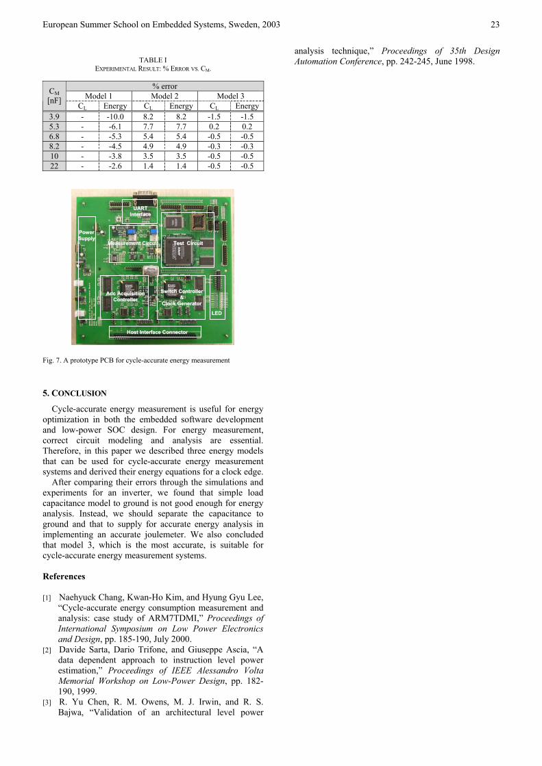
European Summer School on Embedded Systems, Sweden, 2003 23
TABLE I
EXPERIMENTAL RESULT: % ERROR VS. CM. % error
Model 1 Model 2 Model 3 CM [nF]
CL Energy CL Energy CL Energy3.9 - -10.0 8.2 8.2 -1.5 -1.5 5.3 - -6.1 7.7 7.7 0.2 0.2 6.8 - -5.3 5.4 5.4 -0.5 -0.5 8.2 - -4.5 4.9 4.9 -0.3 -0.3 10 - -3.8 3.5 3.5 -0.5 -0.5 22 - -2.6 1.4 1.4 -0.5 -0.5
Host Interface ConnectorHost Interface Connector
Adc Adc AcquisitionAcquisitionControllerController
Switch ControllerSwitch Controller&&
Clock GeneratorClock Generator
LEDLED
Measurement CircuitMeasurement Circuit Test CircuitTest Circuit
UARTUARTInterfaceInterface
PowerPowerSupplySupply
Host Interface ConnectorHost Interface Connector
Adc Adc AcquisitionAcquisitionControllerController
Switch ControllerSwitch Controller&&
Clock GeneratorClock Generator
LEDLED
Measurement CircuitMeasurement Circuit Test CircuitTest Circuit
UARTUARTInterfaceInterface
PowerPowerSupplySupply
Fig. 7. A prototype PCB for cycle-accurate energy measurement
5. CONCLUSION Cycle-accurate energy measurement is useful for energy
optimization in both the embedded software development and low-power SOC design. For energy measurement, correct circuit modeling and analysis are essential. Therefore, in this paper we described three energy models that can be used for cycle-accurate energy measurement systems and derived their energy equations for a clock edge.
After comparing their errors through the simulations and experiments for an inverter, we found that simple load capacitance model to ground is not good enough for energy analysis. Instead, we should separate the capacitance to ground and that to supply for accurate energy analysis in implementing an accurate joulemeter. We also concluded that model 3, which is the most accurate, is suitable for cycle-accurate energy measurement systems.
References
[1] Naehyuck Chang, Kwan-Ho Kim, and Hyung Gyu Lee,
“Cycle-accurate energy consumption measurement and analysis: case study of ARM7TDMI,” Proceedings of International Symposium on Low Power Electronics and Design, pp. 185-190, July 2000.
[2] Davide Sarta, Dario Trifone, and Giuseppe Ascia, “A data dependent approach to instruction level power estimation,” Proceedings of IEEE Alessandro Volta Memorial Workshop on Low-Power Design, pp. 182-190, 1999.
[3] R. Yu Chen, R. M. Owens, M. J. Irwin, and R. S. Bajwa, “Validation of an architectural level power
analysis technique,” Proceedings of 35th Design Automation Conference, pp. 242-245, June 1998.
European Summer School on Embedded Systems, Sweden, 2003 24
Event-Driven Energy Characterization Frank Bellosa
Abstract—Embedded hardware monitors in the form of event counters have proven to offer valuable information in the field of performance analysis. We will demonstrate that counter values can also reveal the power-specific characteristics of a thread. A recurrent analysis of the thread-specific energy and performance profile allows the operating system an adjustment of the power consumption to the behavioral changes of the application. The adjustment can be done with respect to the demands of individual applications, users or services.
The lecture gives two examples for OS-directed power management on the level of threads:
An energy-aware scheduling policy for non-real-time operating systems is proposed which benefits from event counters. By exploiting the information from these counters, the scheduler determines the appropriate clock frequency for each individual thread according to the performance requirements. This adaptive clock scaling is accomplished by the operating system without any application support. Energy measurements of a low-power architecture under variable load show the advantage of the proposed approach.
Another use case for event-driven energy characterization is dynamic thermal management. The lecture describes a model to determine the energy consumption of individual threads and to estimate the temperature of a high-power processor without the need for measurement.
This power and thermal model is combined with the well-known facility of resource containers to throttle the execution of individual tasks according to their energy-specific characteristics and the thermal requirements of the system.
Experiments show that a given temperature limit for the CPU will not be exceeded while tasks are scheduled according to their attached resource containers.
Index Terms — Operating Systems, scheduling, power management, frequency scaling, thermal management
I. INTRODUCTION
To meet the insatiable demand for high performance hardware, components with increased gate count and
clock frequency were developed. The improvements in manufacturing processes could not keep the power increase at a reasonable level. With the emergence of portable devices and the thermal problems of high power processors we are suddenly facing a rising awareness for the topic of energy management.
This lecture contributes to this awareness and presents a new approach in system software: the on-line evaluation of counters that register performance- and energy-critical events. We will show that there is not only a correlation between events and performance but also between events and power consumption. By exploiting these counters the operating system has the complete knowledge Manuscript received January 31, 2004 F. Bellosa is with the University of Erlangen, Germany (e-mail: bellosa@ cs.fau.de).
where the energy has been consumed, where the time has been spent, and who has been responsible for the use of energy.
According to the individual demands of each application, power management can find a trade-off between energy consumption, energy efficiency and quality of service demands. To fulfill this task an operating system has a variety of options for the activation and configuration of energy-critical hardware components. Not only the time of activation but also the degree of activation (e.g., the clock speed of a processor) can be controlled. The next sections describe the benefit of event driven energy characterization for improving the energy efficiency of processors with variable clock speed and for dynamic thermal management of high performance processors.
II. PROCESS CRUISE CONTROL Performance and energy consumption at variable speeds
are two characteristics which are correlated, but the degree of correlation depends on the use of performance- and energy-critical hardware components. Only if the operating system knows the specific usage patterns of each of the managed execution entities (threads or processes), it can find the best energy/performance trade-off and select the right speed of execution [4].
A. The Policy Model Our approach to find the patterns is the on-line evaluation
of event-counters [8]. For a specific architecture we have to find a set of countable events that characterize the behaviour of a thread concerning performance and energy consumption when the thread is executed at various clock frequencies. The rates at which these events can happen at a certain clock frequency span a multidimensional space which describes all the potential patterns a thread could exhibit.
For each point in the space we can find the proper clock frequency that minimizes the energy consumption for a given performance requirement.
We are facing the challenge to partition this space into domains with equal clock frequency and to describe these partitions (frequency domains) in a way that the scheduler of the operating system can determine the clock speed of a specific thread by a fast mapping from event rates to clock frequencies. The optimal speeds for the various event rates and, consequently, the resulting partitions depend on the restriction in performance loss. The current set of partitions defines the model policy.

European Summer School on Embedded Systems, Sweden, 2003 25
Figure 1: Process Cruise Control loop
A scheduler implementing Process Cruise Control adapts the clock speed when switching from one thread to another. The new frequency is determined by a periodic evaluation of the event rates in the latest history of the thread. Therefore the scheduler has to find the frequency domain that matches all the event rates of the thread. We saw that while the energy specific characteristics of a single thread change only slowly over time, the characteristics of concurrently running threads alter frequently and show a wide variation. For a single thread it is sufficient to analyze the behaviour of this thread at each context switch. Our approach respects the variation in behaviour by adapting the clock speed at each thread switch according to the characteristics of this thread. This guarantees an optimal speed adaptation.
The data flow in figure 1 shows the relation of the Process Cruise Control model to a car cruise control or any other controlled system. Sampled event rates along with corresponding execution speeds run into the model policy.
An optimal speed prognosis is made and applied to the application. Again, the new CPU speed is fed into the model along with newly measured event rates closing the loop of control.
To summarize, our approach can be outlined as follows: Determine the correlation between the rates of different events and both performance and energy consumption. Identify the lowest possible clock frequency (the optimal speed) for a certain combination of event rates under an user-specified upper bound for performance degradation. On each task-switch, scale the clock frequency according to the pre-computed optimal speed for the thread specific event rates.
B. XScale Frequency Domains The Intel XScale 80200 processor used in an Intel
IQ80310 evaluation board implements one clock and two event counters. Under these restrictions, the selection of the following events is recommended: The memory requests per clock cycle clearly indicate the degree of memory use. The higher the rate of memory requests the more the energy performance will benefit from a reduction in clock speed as the processor does not waste energy for memory stall cycles. The instructions per clock cycle indicate the sensitivity for a performance loss due to speed reduction. The lower the rate of executed instructions is the less the performance of a thread will suffer from a reduction in clock speed.
Cache misses as an indicator for energy consumption can not be used because several event counters for all types of energy-relevant cache events are not available on the target architecture. Furthermore several counters for different cache events would have to be monitored in parallel. Therefore we used the counter for memory requests because they showed the best correlation to energy consumption.
eventrates
model policyapplicationcurrent
CPU speed
set newCPU speed
To span the space of both event rates we constructed micro benchmarks producing various event rates. For each clock speed, we determined the event rates for each of these benchmarks. The next step is to find the minimal clock speed which can be tolerated for given performance requirements.
For our tests we chose 10% as an acceptable performance loss. The last step is to partition the two-dimensional space into frequency domains.
1.5%
0.5%
1.0%
2.0%
2.5%
3.0%
100%80%60%40%20%0%
333 MHz
400 MHz
466 MHz
533 MHz
600 MHz
733 MHz
666 MHz
mem
ory
requ
ests
/ cl
ock
cycl
e
instructions / clock cycleFigure 2: XScale frequency domains for Intel IQ80310
We chose a simple approach with matrices that define the
frequency domains (for an example see figure 2). The dimensions of the matrix are the event rates, the percentage of instructions per cycle, ranging from 0% to 100%, and the percentage of memory requests per cycle, ranging from 0% to 3% (this is the maximum value achievable by artificial micro benchmarks). A simple matrix look-up operation yields the optimal clock speed.
C. Measurements To show the benefits of event-driven clock scaling we
measured the energy consumption and performance of five well known applications to find the optimal clock speed according to external energy measurements and to compare the optimal frequency with the results of process cruise control. We ran these five applications at all possible clock frequencies to determine the energy consumption, performance and clock speed according to an allowed penalty of 10% performance loss.

European Summer School on Embedded Systems, Sweden, 2003 26
We could prove that it is possible to come very close to the
optimal clock frequency by an on-line evaluation of event counters. For three applications process cruise control determined the optimal clock speed. One application (djpeg) is scheduled with a speed that is just one step to low. The runtime behavior of the postscript interpreter is influenced by the content of the postscript file to convert. Therefore the frequency switching pattern of the process run depends on the content and structure of the input file and varies between 400 MHz and 600 MHz.
For the Intel IQ80310 system energy savings of 15% are possible without severe performance impact. If we tolerated a higher performance degradation, the energy efficiency could be improved further.
D. Limitations The selection of countable events was done to support
performance profiling and not energy profiling. Several events which differ substantially in their energy consumption cannot be differentiated. An example are read and write memory requests which differ in their energy characteristics.
The qualitative characterization of Cruise Control using just two counters was sufficient for best-effort optimization of the energy consumption, however it is inadequate for quantitative guarantees which require the sampling of many more energy-critical events.
III. DYNAMIC THERMAL MANAGEMENT Control-theoretic techniques have proven to manage the
heat dissipation and temperature starting from the level of functional blocks within the processor up to the level of complete systems, so that a thermal emergency will never be reached [7]. However application-, user- or service-specific requirements had to be neglected. The reason is not so much a lack of fast acting thermal response mechanisms but missing on-line information about the originator of a specific hardware activation and the amount of energy consumed by that activity.
In this lecture, we present an event-driven energy-esti-mation model that employs event-monitoring counters to determine on-the-fly the actual power consumption and who has used the power in the system. With the specification of the cooling system (thermal resistance and capacitance), the temperature can be estimated without the need for measurement and used to trigger task-specific throttling. The event-driven power and thermal model is combined with the facility of resource containers [1] to throttle the execution of individual tasks according to their energy-specific characteristics, their service requirements and the thermal
demands of the system. We call this operating system abstraction Energy Containers. Additionally we present a CPU scheduler which identifies and penalizes “hot” processes by reducing their time slices.
process cruise control: application optimal speed
clock scaling energy savings
find | grep 400 MHz 400 MHz 15 %
gzip 466 MHz 466 MHz 10 %
djpeg 600 MHz 533 MHz 8 %
factor 600 MHz 600 MHz 4 %
ghostscript 400MHz – 600 MHz 5 %
Two target application spaces benefit from dynamic thermal management: in the server market, cooling facilities play a significant role in the overall power consumption and costs. Furthermore, cooling facilities are often overprovisioned in order to cope with a cooling unit failure. In the laptop market, dynamic thermal management could make fans obsolete or at least limit the power consumption
used for cooling and, as a consequence, achieve longer battery lifetime.
A. Event-Driven Energy Estimation The increasing complexity of modern processors (super-
scalar architecture, out of order execution, branch pre-diction, ...) demands a more elaborate procedure to estimate on-the-fly the power consumption. While it was sufficient for former architectures like Pentium II to calculate the percentage of CPU activity [6], we registered a wide variation of the active power consumption between 30 W and 51 W for the P4 architecture running a compute intensive task. We measured the power and energy consumption of a set of test programs structured in three groups (see bars in figure 3):
Figure 3: Measured and estimated power consumption ALU: programs which operate entirely on registers using ALU instructions like addc, bswap, xor, ... MEM: programs which operate on registers and memory (including L1/L2 caches) Micro benchmarks which perform various algorithms (checksum, factor, heron, SHA-1, RIPEMD-160, ...). Because there are high-power tasks that need about 70%
more power than low-power tasks, CPU cycles are no longer a clear indicator for energy consumption.
The next step is to use more processor-internal information provided by the performance counters on-line. Modern processors feature much more performance counters than their predecessors. In particular, the Pentium 4 architecture provides 18 performance counters which can be used simultaneously. Our approach to energy estimation is to correlate a processor-internal event to an amount of energy. As events
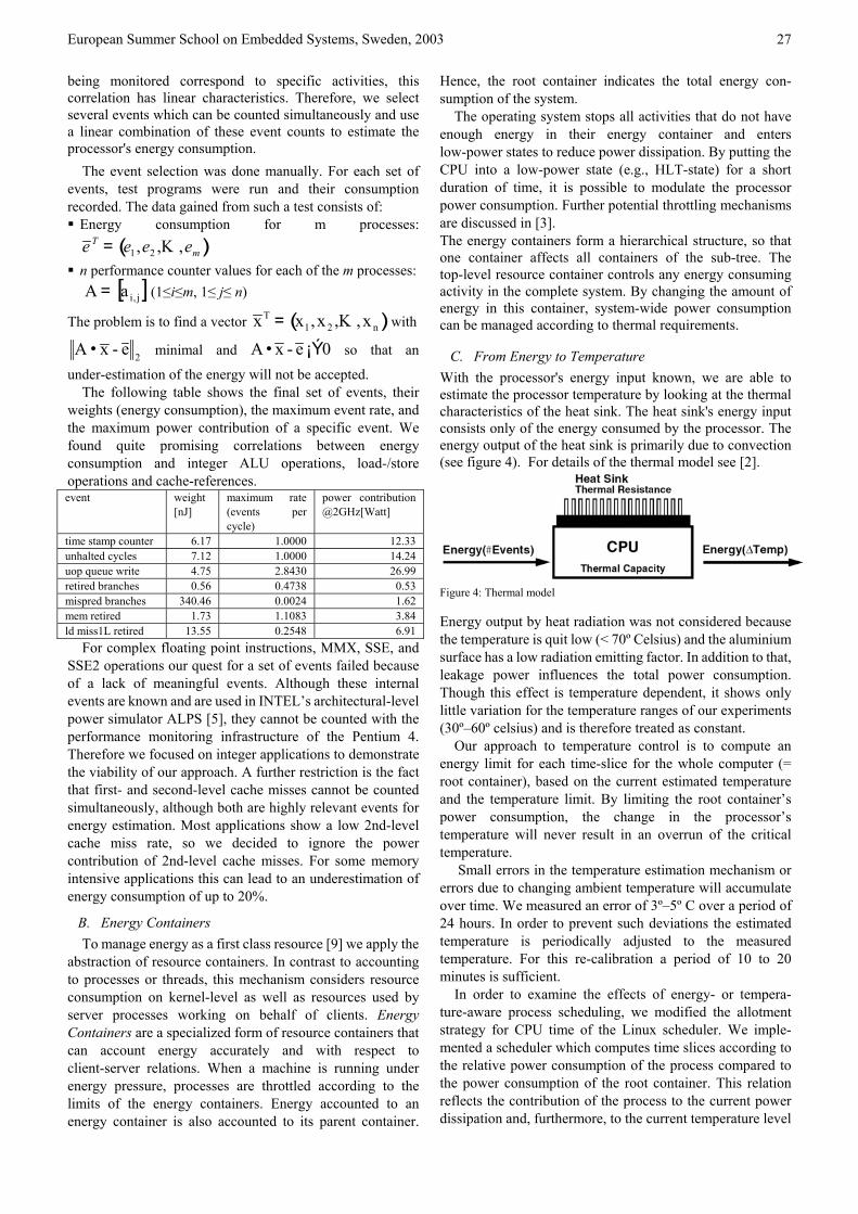
European Summer School on Embedded Systems, Sweden, 2003 27
being monitored correspond to specific activities, this correlation has linear characteristics. Therefore, we select several events which can be counted simultaneously and use a linear combination of these event counts to estimate the processor's energy consumption.
The event selection was done manually. For each set of events, test programs were run and their consumption recorded. The data gained from such a test consists of: Energy consumption for m processes:
( )mT eeee ,,, 21 Κ=
n performance counter values for each of the m processes: [ ]j,iaA = (1≤i≤m, 1≤ j≤ n)
The problem is to find a vector ( n21T x,,x,xx Κ= ) with
2e-xA • minimal and 0e-xA ¡Ý• so that an
under-estimation of the energy will not be accepted. The following table shows the final set of events, their
weights (energy consumption), the maximum event rate, and the maximum power contribution of a specific event. We found quite promising correlations between energy consumption and integer ALU operations, load-/store operations and cache-references. event weight
[nJ] maximum rate (events per cycle)
power contribution@2GHz[Watt]
time stamp counter 6.17 1.0000 12.33unhalted cycles 7.12 1.0000 14.24uop queue write 4.75 2.8430 26.99retired branches 0.56 0.4738 0.53mispred branches 340.46 0.0024 1.62mem retired 1.73 1.1083 3.84ld miss1L retired 13.55 0.2548 6.91
For complex floating point instructions, MMX, SSE, and SSE2 operations our quest for a set of events failed because of a lack of meaningful events. Although these internal events are known and are used in INTEL’s architectural-level power simulator ALPS [5], they cannot be counted with the performance monitoring infrastructure of the Pentium 4. Therefore we focused on integer applications to demonstrate the viability of our approach. A further restriction is the fact that first- and second-level cache misses cannot be counted simultaneously, although both are highly relevant events for energy estimation. Most applications show a low 2nd-level cache miss rate, so we decided to ignore the power contribution of 2nd-level cache misses. For some memory intensive applications this can lead to an underestimation of energy consumption of up to 20%.
B. Energy Containers To manage energy as a first class resource [9] we apply the
abstraction of resource containers. In contrast to accounting to processes or threads, this mechanism considers resource consumption on kernel-level as well as resources used by server processes working on behalf of clients. Energy Containers are a specialized form of resource containers that can account energy accurately and with respect to client-server relations. When a machine is running under energy pressure, processes are throttled according to the limits of the energy containers. Energy accounted to an energy container is also accounted to its parent container.
Hence, the root container indicates the total energy con-sumption of the system.
The operating system stops all activities that do not have enough energy in their energy container and enters low-power states to reduce power dissipation. By putting the CPU into a low-power state (e.g., HLT-state) for a short duration of time, it is possible to modulate the processor power consumption. Further potential throttling mechanisms are discussed in [3]. The energy containers form a hierarchical structure, so that one container affects all containers of the sub-tree. The top-level resource container controls any energy consuming activity in the complete system. By changing the amount of energy in this container, system-wide power consumption can be managed according to thermal requirements.
C. From Energy to Temperature With the processor's energy input known, we are able to estimate the processor temperature by looking at the thermal characteristics of the heat sink. The heat sink's energy input consists only of the energy consumed by the processor. The energy output of the heat sink is primarily due to convection (see figure 4). For details of the thermal model see [2].
Figure 4: Thermal model Energy output by heat radiation was not considered because the temperature is quit low (< 70º Celsius) and the aluminium surface has a low radiation emitting factor. In addition to that, leakage power influences the total power consumption. Though this effect is temperature dependent, it shows only little variation for the temperature ranges of our experiments (30º–60º celsius) and is therefore treated as constant.
Our approach to temperature control is to compute an energy limit for each time-slice for the whole computer (= root container), based on the current estimated temperature and the temperature limit. By limiting the root container’s power consumption, the change in the processor’s temperature will never result in an overrun of the critical temperature.
Small errors in the temperature estimation mechanism or errors due to changing ambient temperature will accumulate over time. We measured an error of 3º–5º C over a period of 24 hours. In order to prevent such deviations the estimated temperature is periodically adjusted to the measured temperature. For this re-calibration a period of 10 to 20 minutes is sufficient.
In order to examine the effects of energy- or tempera-ture-aware process scheduling, we modified the allotment strategy for CPU time of the Linux scheduler. We imple-mented a scheduler which computes time slices according to the relative power consumption of the process compared to the power consumption of the root container. This relation reflects the contribution of the process to the current power dissipation and, furthermore, to the current temperature level

European Summer School on Embedded Systems, Sweden, 2003 28
of the CPU. Additionally, the priority computation—the decision which process will run next—is based on the relative power consumption. With this approach “hot” processes are disadvantaged by the scheduler.
To sum up, we are able to identify hot processes using energy containers. We present two means to deal with them: first, limiting the power consumption of the attached containers automatically throttles hot processes as they spend their power budget faster than the others. Second, a power-based process scheduler can allot longer time slices to energy-efficient processes. While the second approach does not waste CPU time, throttling is needed to facilitate thermal management.
D. Evaluation The effect of throttling can be illustrated with a web server
accepting requests from two different classes of clients. When a critical temperature limit of 50º Celsius is reached, client #1 should be preferred and should get a share of 80% of the allowed total power, while client #2 is just allowed to consume 20% of the remaining power. Figure 5 shows the power consumption of the free running apache tasks working on behalf of the two classes of clients before and after reaching the predefined limit of 50º Celsius. The root container reflects the sum of both client containers plus the power consumption of the halted CPU accounted to the idle thread.
Figure 5: Throttling at 50º according to energy shares
Reading of the event-monitoring counters in a Linux 2.5 is done in the timer interrupt (1000 times per second) or when a task is blocking. The context switching times with energy container support is increased by 49% (5.9 µs) due to algorithmic overhead and the time for reading the event counters. However for a typical scenario like kernel compiling we registered an overall performance loss of less than 1% (the time a kernel compile run needs on the original kernel compared to our modified kernel).
Estimating the temperature takes about 5 µs while setting new limits to the root container requires 12. The overhead for temperature estimation can be neglected because this procedure is typically executed 1-10 times per second. Furthermore, the overhead is by orders of magnitude smaller compared to reading the temperature sensors of the motherboard (which takes about 5.5 ms).
E. Conclusion Event-monitoring counters are the adequate source of
information for on-the-fly energy characterization. Restricting our validation to integer applications we could demonstrate the benefit of performance monitoring counters for finding the appropriate clock frequency, for an estimation of energy consumption, and for managing the processor temperature. We expect thread-specific throttling and speed settings in combination with event-driven energy profiling to become an essential element of future operating systems for power-sensitive devices.
REFERENCES [1] G. Banga, P. Druschel, and J. Mogul, “Resource containers: A new
facility for resource management in server systems,” in Proc. Third Symposium on Operating System Design and Implementation OSDI’99, February 1999.
[2] F. Bellosa, A. Weissel, M. Waitz, and S. Kellner, “Event-driven energy accounting for dynamic thermal management,” in Proc. Workshop on Compilers and Operating Systems for Low Power (COLP'03), September 2003.
[3] D. Brooks and M. Martonosi, “Dynamic thermal management for high-performance microprocessors,” in Proc. Seventh International Symposium On High-Performance Computer Architecture (HPCA’01), January 2001.
[4] K. Flautner and T. Mudge, “Vertigo: Automatic performance-setting for linux,” in Proc. Fifth Symposium on Operating System Design and Implementation OSDI'2002, December 2002.
[5] S. H. Gunther, F. Binns, D. M. Carmean, and J. C. Hall. “Managing the impact of increasing microprocessor power consumption,” Intel Technology Journal, 2001. Q1 issue.
[6] E. Rohou and M. Smith, “Dynamically managing processor temperature and power,” in Proc. 2nd Workshop on Feedback-Directed Optimization, November 1999.
[7] K. Skadron, T. Abdelzaher, and M. R. Stan, “Control-theoretic techniques and thermal-rc modeling for accurate and localized dynamic thermal management,” in Proc. Seventh International Symposium On High-Performance Computer Architecture (HPCA’02), January 2002
[8] A. Weissel and F. Bellosa, “Process cruise control: Event-driven clock scaling for dynamic power management,” in Proc. International Conference on Compilers, Architecture, and Synthesis for Embedded Systems CASES'02, October 2002.
[9] H. Zeng, X. Fan, C. Ellis, A. Lebeck, and A. Vahdat., “Ecosystem: Managing energy as a first class operating system resource,” in Proc. Tenth International Conference on Architectural Support for Programming Languages and Operating Systems ASPLOS’02, October 2002
Frank Bellosa is an assistant professor in the Department of Computer Science at the University of Erlangen. His research interests are in operating systems, energy-efficient designs, and computer architecture. Bellosa received a PhD in computer science from the University of Erlangen. He is a member of the ACM and the German Informatics Society (GI). Contact him at [email protected].

European Summer School on Embedded Systems, Sweden, 2003
29
Operating System Design for Energy Management
Carla Schlatter Ellis, Alvin R. Lebeck, Xiaobo Fan, Angela Dalton, and Heng Zeng
Abstract—Energy is an increasingly important system
resource in battery-powered mobile computing platforms. The Milly Watt Project at Duke University advocates managing energy as a first-class operating system resource. Our initial focus has been on the operating system design without mandating that applications must become energy-aware in order to benefit. In our ECOSystem framework, energy use is represented by the Currentcy Model. This abstraction provides a powerful mechanism to formulate energy goals and to unify resource management policies across competing applications and multiple device components with very different power characteristics. The ECOSystem prototype demonstrates how the processor, disk, and wireless network interface of a laptop computer can be managed together to achieve a target battery lifetime. Although not yet incorporated into the ECOSystem framework, we also consider techniques for managing other important system devices, namely main memory and the display.
Index Terms—operating systems, battery lifetime, mobile
computing devices, energy management.
I. INTRODUCTION
ENERGY is an increasingly important system resource in battery-powered mobile computing platforms, from laptops to tiny embedded sensor nodes. The Milly Watt
Project has advocated that energy be explicitly treated as a first-class operating system managed resource [1]. Energy has a system-wide impact on the computing platform and the operating system is traditionally responsible for the system-wide management of resource supply and demand. Our challenge has been to explore what the OS can do to unify the management of a diverse set of resources under an umbrella of energy, achieve specified energy-related goals, and not require all applications to become energy-aware in order to derive benefits. Related work on application adaptation (e.g., [2]) is valuable and complementary to our approach. There has been considerable work on managing the energy use of individual devices, for example, CPU voltage scaling, disk spindown policies, and energy-aware networking. Our work is distinguished by its system-wide treatment of energy as a first-class resource. In this short paper, we describe our ECOSystem design
that elevates energy to a central place in the resource management of the system [3, 4]. We describe the Currentcy Model 1 that captures the power characteristics of device components and provides an energy abstraction for allocation and accounting. The ECOSystem prototype provides experimental evidence of the effectiveness of our approach. Although not yet incorporated into the ECOSystem framework, we also present techniques for managing main memory and the display.
Manuscript received January 31, 2004. This work was supported in part by the National Science Foundation under awards EIA-9986024, ITR-00082914, CCR-0208920, and 0204367. For more information: http://www.cs.duke.edu/ari/millywatt.
Carla Schlatter Ellis is with Duke University, Durham, NC 27708-0129, USA (919-660-6523; fax: 919-660-6519; e-mail: [email protected]). Alvin R. Lebeck ([email protected]), Xiaobo Fan ([email protected]), Angela Dalton ([email protected]), and Heng Zeng ([email protected]) are also with Duke University, Durham NC 27708-0129, USA.
II. THE ECOSYSTEM FRAMEWORK
A. The Currentcy Model The key feature of our model is the use of a common
unit— currentcy—for energy accounting and allocation across a variety of hardware components and tasks. Currentcy becomes the basis for characterizing the power requirements and gaining access to any of the managed hardware resources. It is the mechanism for establishing a particular level of power consumption and for sharing the available energy among competing tasks.
The target battery lifetime and our battery model are used to determine an appropriate level of current and this is translated into an amount of currentcy that can be made available during each epoch of time. This currentcy allocation is distributed to the competing tasks according to their specified proportional shares. Each task uses its currentcy allowance to gain access to devices. Each device has a pricing policy for deducting currentcy that reflects its current power mode and transitions. The calibrated power model embedded in the system tracks the power state transitions for each managed device and allows accurate
Figure 1 Currentcy Flow. Target battery lifetime determines overall currentcy allocation for an epoch (1), task shares determine per-task allocations (2), and device accounting policies deduct currentcy from task budgets (3).
1 Currentcy is a coined term, combining the concepts of current (i.e., amps) and currency (i.e., $).

European Summer School on Embedded Systems, Sweden, 2003
30
accounting to the tasks responsible for the device activity.
B. ECOSystem Prototype The ECOSystem (Energy Centric Operating System)
prototype is a modified RedHat Linux version 2.4.0-test9 running on an IBM ThinkPad T20 laptop. This platform has a 655MHz PIII processor and we assume an active power consumption of 15.55W. The disk is an IBM Travelstar that we model in ECOSystem with costs of 1.65mJ per block access and 6000mJ for both spinup and spindown, and with progressive costs/timeouts for levels of idle power states. The wireless network is an Orinoco Silver PC card supporting IEEE 802.11b. It has three power modes: Doze (0.045W), Receive (0.925W) and Transmit (1.425W). All other devices contribute to the base power consumption, measured to be 13W for the platform. There is a simple user interface to set the target battery lifetime and set task shares. There is a new kernel thread kenrgd that wakes up periodically and distributes currentcy appropriately.
C. Exploration of the Policy Space The Currentcy Model framework and the ECOSystem
prototype serve as a testbed for exploring the range of policies that can be expressed in terms of currentcy. Without some abstraction like currentcy, there is no language in which to explicitly formulate desired energy-related behaviors and solutions.
Our initial, basic policies are simply pay-as-you-go [3]. A task can gain access to a managed device as long as it has currentcy to pay for the request. Consider processor scheduling as an example: Ready-to-run tasks with currentcy remaining can be scheduled for a timeslice. When there are no tasks with any currentcy left, even though they may be otherwise runnable, the processor is halted until the next epoch’s allocation. Without assuming adaptation by the application, this seems a reasonable way to throttle back service to meet the energy goal. Using feedback from a smart battery interface, the allocations can be adjusted to correct for modeling errors. I/O requests that cause disk activity result in currentcy being deducted from the responsible task with the cost of spinning up and down the disk shared by all tasks using the disk during the period between spinup and spindown.
Subsequent policies [4] have been designed to address more elaborate behaviors and solve some performance problems that arise in these simple policies. We consider four new goals: 1) reducing residual battery capacity at the end of the targeted battery lifetime when it is no longer needed, 2) dynamic tracking of the energy needs of competing applications for more effective energy sharing, 3) reducing response time variation caused by limited energy availability, and 4) energy efficient disk management. We have developed a currentcy conserving allocation policy to reclaim unspent energy by adapting to energy consumption patterns which are made observable by the currentcy abstraction. We have developed a currentcy-based scheduling policy that recognizes the global relevance of energy consumption anywhere in the system on the scheduling decision, resulting in more robust proportional sharing of energy. We further enhance that scheduling policy
to pace the energy consumption, thus reducing response time variation. Finally, we demonstrate how to shape disk access patterns to amortize the energy costs of spinup/spindown across multiple requests and thereby reduce the average energy used per request. We also show the energy and performance benefits of aggressive prefetching while the disk is already spinning.
D. Experimental Results To investigate the impact of energy accounting
inaccuracies, we use a CPU-intensive microbenchmark, but deliberately introduce an accounting error for the CPU power consumption (14W instead of the measured 15.55W). Each experiment with different target lifetimes is run until the battery is depleted. Figure 2 shows the target battery lifetime on the x-axis and the achieved battery lifetime on the y-axis. One curve demonstrates the behavior of the system without correction, in this case continuously missing the target battery lifetime by approximately 10%. Finally, another curve on the graph shows that with our periodic corrections, we are able to achieve the target despite the deliberately introduced error. We conclude that ECOSystem is successful at managing the battery lifetime.
Currentcy conserving allocation allows the system to redistribute currentcy allocations from tasks that have more than they need to tasks that can use more. The problem arises when tasks that are entitled to large currentcy allocations but
are unable to consume their entire allocations (e.g., during think time) essentially throw away their unspent currentcy. To evaluate the benefits of currentcy conservation, we use a workload consisting of a gqview image viewer and ijpeg. Gqview is set to autobrowse mode where it continuously loads each of 12 images in a directory with a 10 second “think time” pause between each image. The computationally intensive ijpeg is run in a loop to continuously encode and decode an image residing in memory. The overall currentcy allocation is equivalent to 12000mW with 8000mw for gqview and 4000mW for ijpeg. With its think time, gqview can only use an average of 7000mW whereas the computationally intensive ijpeg can easily consume up to 15.5W in the processor.
Figure 2 Achieving a target battery lifetime. With feedback from the smart battery, the achieved battery lifetime matches the target lifetime in spite of accounting errors.

European Summer School on Embedded Systems, Sweden, 2003
31
Figure 3 shows the power consumption in each epoch over a 100 second time interval. This shows that when gqview is idle (i.e., during “think” time with zero power consumption), ijpeg can consume maximum CPU power. However, when gqview is active, ijpeg is limited to its 4000mW allocation. There is little energy capacity remaining when the battery lifetime is reached (less than 1%).
E
eOpptciop
A
cgyibMtma
ctTpm
i
respond to observable memory access patterns. We have explored controller policies that are based on the idle time between runs of accesses (which we refer to as gaps) and threshold values to trigger transitions [5]. Figure 4 illustrates a policy that transitions between active and powerdown modes. While the memory has outstanding requests, the memory chip stays active. Upon the completion of those requests, the chip automatically goes to standby. When the idle time exceeds a threshold (e.g., gap i), the chip transitions into powerdown and stays there until the start of the next access (the end of the gap). For gaps shorter than the threshold (e.g., gap j), the memory remains in standby.
Our results, based on simulation and analysis, have
Figure 3 Currentcy conserving allocation. The three horizontal linesrepresent (from top to bottom) the total allocation, the allocation forgqview, and the allocation for ijpeg. At point A, gqview is active, soijpeg is limited to its allocation. At point B, gqview is in its think time, soijpeg can benefit from its unused currentcy.
. Summary ECOSystem continues to provide a productive
nvironment for investigating unified energy management. ur results so far have shown that the currentcy model is a owerful framework for expressing energy management olicies and that our currentcy-based policies, by being able o capture aspects of global energy use, can provide more oherency to system-wide energy management. We plan to ncorporate more components into the explicitly managed set f devices and experiment with other energy-related roblems.
III. ENERGY MANAGEMENT FOR MEMORY
. Power-Aware DRAM Technology In addition to components that our ECOSystem prototype
an manage on existing laptop platforms, the Milly Watt roup has considered emerging technologies that have not et become widely integrated into products. With the recent ntroduction of DRAM chips that allow transitioning etween power states (e.g., Rambus RDRAM and Intel obile-RAM), there are opportunities to consider the role of
he operating system in the energy management of main emory. First, we introduce the hardware characteristics we
ssume. Power-aware memory chips can transition into states that
onsume less power but introduce additional latency to ransition back into the active state in order to be accessed. he lower the power consumption associated with a articular state, the higher the latency to service a new emory request. The memory controller can exploit these states by
mplementing dynamic power state transition policies that
exgihais
pohatesc
B.
staopvipasim
chasfebetopoinreapimtrapr
Figure 4 Memory access behavior. This shows the relationship of thresholds, gaps, and state transitions in a 2-state memory controller policy.
plored how to determine the best threshold values [6, 7] ven the gap distribution from a particular workload. We ve found that in many cases, a good static threshold policy to transition immediately (i.e., a threshold equal to zero). We have also investigated the synergy between wer-aware memory and dynamic voltage scaling [8]. We ve shown that the interaction between these two chnologies affects both memory controller policies and heduling policies.
The Role of the OS: Power-Aware Page Allocation Given dynamic memory controllers managing the power tes of the memory chip, we next consider how the erating system can facilitate better energy efficiency. The rtual to physical page mapping can be tailored to cluster ges into the fewest number of chips or with pages of ilar access patterns or activity levels.
Our study of page placement policies [5] assumes the aracteristics of Rambus DRAM – the power states as well the high bandwidth possible from a single chip. This ature allows pages to reside within a single chip rather than interleaved across chips. In this context, sequential first uch page allocation in conjunction with memory controller licies that dynamically adjust the power mode of each dividual chip independently produces dramatic simulation sults. For a set of memory traces from popular productivity plications and from SPEC benchmarks, we have found provements of 80-99% in an energy*delay metric over ditional full-powered memory devices. Related work [9] oposes that the OS do the transitions at a context switch.

European Summer School on Embedded Systems, Sweden, 2003
32
IV. DISPLAY MANAGEMENT
A. The FaceOff Design The display is another major consumer of power in a
typical battery-powered device. The display exists solely for the purpose of user interaction and therefore it is only necessary when someone is looking at it. There are many times when a user may turn her attention away from the computer display, perhaps to answer a phone call or to focus on some other distraction. On the other hand the conventional display power management scheme that is based on a timeout from a lack of user input events may be too aggressive for some applications. A user reading an electronic book or examining a web page with complex content might experience the annoying behavior of the display timing out.
Based on the simple intuitive idea that the display is not needed if no one is looking at it, we evaluate our power management method, called FaceOff, that uses a web cam mounted to the display of a laptop as a sensor [10]. The camera periodically captures images and a face detection algorithm determines the presence or absence of a user looking at the display. The display is turned off and back on based on the results of the face detection. Detecting an area of skin color in the image has proved adequate for our purposes.
B. Prototype and Preliminary Results We have built the FaceOff prototype on an IBM T21
Thinkpad running Red Hat Linux. The camera is a color Logitech QuickCam 3000 web cam that connects via USB to the laptop with an average measured power consumption of 1.5W. The display power states are defined in the ACPI specification and supported by both the laptop hardware and the operating system. On this laptop, the display consumes approximately 8.5W. In the future, FaceOff will be integrated into ECOSystem.
Preliminary experiments with our prototype have been done to determine whether this method can produce a measurable reduction of energy consumption in the system even after accounting for the added computing energy costs for the face detection algorithm and the energy consumed by the camera. The results are encouraging. The addition of a very low power motion sensor is proposed to avoid overhead during long user absences. Future work will study the user’s experience with FaceOff.
V. CONCLUSION ECOSystem, power-aware page allocation, and FaceOff
span the typical components of a mobile computing platform. Our goal is to take a system-wide view and show that unifying resource management in terms of energy management is a promising approach.
REFERENCES [1] A. Vahdat, C. Ellis, and A. Lebeck. “Every Joule is Precious: The Case
for Revisiting Operating System Design for Energy Efficiency” in Proceedings of the 9th ACM SIGOPS European Workshop, September 2000.
[2] J. Flinn and M. Satyanarayanan. “Energy-aware adaptation for mobile applications” in Symposium on Operating Systems Principles (SOSP), pages 48–63, December 1999.
[3] Heng Zeng, Carla S. Ellis, Alvin R. Lebeck, and Amin Vahdat. “Ecosystem: Managing energy as a first class operating system resource” in Proceedings of the Tenth International Conference on Architectural Support for Programming Languages and Operating Systems (ASPLOSX), page 123, October 2002.
[4] Heng Zeng, Carla S. Ellis, Alvin R. Lebeck, and Amin Vahdat. “Currentcy: a unifying abstraction for expressing energy management policies” in Proceedings of the USENIX Annual Technical Conference, June 2003.
[5] Alvin Lebeck, Xiaobo Fan, Heng Zeng, and Carla Ellis, “Power aware page allocation” in Proceedings of the Ninth International Conference on Architectural Support for Programming Languages and Operating Systems (ASPLOSX), November 2000.
[6] Xiaobo Fan, Carla. Ellis, and Alvin Lebeck, “Memory Controller Policies for DRAM Power Management” in Proceedings of the International Symposium on Low Power Electronics and Design (ISLPED) August, 2001.
[7] Xiaobo Fan, Carla Ellis, and Alvin Lebeck, “General and efficient power management for non-scalable devices”, Duke University technical report, 2003.
[8] Xiaobo Fan, Carla S. Ellis, and Alvin R. Lebeck, “Synergy between Power-aware Memory Systems and Processor Voltage Scaling” in Proceedings of the Workshop on Power-aware Computing Systems (PACS), Dec. 2003.
[9] Huang, Pillai, and Shin, “Design and implementation of power-aware virtual memory” in Proceedings of the USENIX Annual Technical Conference, June 2003.
[10] Angela Dalton and Carla S. Ellis, “Sensing user intention and context for energy management” in Hot Topic on Operating Systems (HOTOS), May 2003.
Modeling and Optimization of Embedded Systemsusing Constraint Programming
Krzysztof Kuchcinski
Abstract— In this paper we briefly discuss embedded computersystems and related design problems. We propose to use con-straint programming methods to solve many of these problemsin a way that is elegant, flexible and efficient at the same time.First, we briefly introduce finite domain constraints and thengive a very simple scheduling and functional units assignmentexample taken from high-level synthesis area. We then provide ashort list of other selected applications for our approach togetherwith related references. Finally, we conclude our discussion bypointing out several advantages of our approach.
Index Terms— Embedded systems, high-level synthesis, systemsynthesis, constraint programming.
I. INTRODUCTION
EMBEDDED computer systems typically perform specificfunctions, such as process control, digital signal pro-
cessing, image processing or multimedia applications. Theyare usually specified by communicating concurrent processesand implemented in software and hardware in a distributedheterogeneous environment. The software is executed on aprocessor or several processors while hardware is usuallyprovided as specialized ASICs. The communication channelsare implemented by buses, point-to-point links or sharedmemories.
An important part of distributed embedded system designspace exploration is partitioning of the system specificationinto processors, ASICs and communication channels as wellas mapping and scheduling of different system functionson available resources. Possible system implementations aresupposed to meet specified performance while providing a costefficient system architecture. Several other constraints, such aspower consumption or fault-tolerance, might be also consid-ered. The design space exploration usually takes into accountpossible system structures, different design constraint as wellas the execution profile of the system together with parameterestimation and tries to find different design alternatives.
Different modeling and optimization approaches have beenproposed for embedded systems. The most common approachis based on different kind of graph-based models. The systemfunctionality is modeled using graphs or more complex for-malism, such as Petri nets. The optimization and design spaceexploration phase is based on different heuristics which areapplied for specific design problems.
Integer Linear Programming (ILP) or Mixed Integer LinearProgramming (MILP) based approaches are also considered.These methods produce optimal solutions while suffering
The author is with the Department of Computer Science, Lund University,Lund, Sweden (e-mail: [email protected]).
usually from long execution times and practical limitation onthe size of the problem. The MILP method requires a carefulformalization of the problem as a set of linear inequalities.Usually, two types of variables are used; system parametervariables, such as timing variables, and binary variables. Whilethe system variables represent real values assigned to systemparameters, the binary variables are introduced to representimplementation decisions regarding the system configuration.The number of the binary variables and the related inequalitiestends to be very large, even for moderate size problems, whichresults in long execution times for finding optimal solutions.
In this paper, a new method for embedded system model-ing and optimization is presented. This method is based onconstraints solving techniques [1]. A system is specified by aset of constraints over the finite domain of integers. The con-straints are given as inequalities and specialized combinatorialconstraints, and specify system constraints as well as resourceconstraints. The constraint solving techniques are then usedto find different solutions, optimal or suboptimal ones, whichsatisfy given constraints and optimize a given cost function. Inour case, in addition to constraint consistency techniques weuse a branch and bound algorithm with depth-first-search orpartial-depth-first-search methods to find a system implemen-tation. The prototype constraint programming system, JaCoP,has been implemented in Java (see, for example [2]) and testedon many examples. This paper summarize our previous studiesand related results which has been published.
Our approach uses extensively constraint programming toaddress different embedded systems design problems rangingfrom partitioning to scheduling and memory assignment. Wemake an extensive use of finite domain constraints withoutlimiting them to linear equations and inequalities. We alsocombine application constraints and resource constraints andpropose a new constraint representation for different designproblems. Finally, we use constraints for design space explo-ration and design optimization. The optimization minimizesan explicitly given cost function while satisfying constraintsset.
The design flow of our approach is depicted in Figure 1. Theconstraints are extracted from a design specification as wellas defined by a designer. Optimization criteria, if needed, arealso defined as constraints. All defined finite domain variables(FDVs) and constraints are then placed in a store that is laterused by a solver to find a solution. The solver uses constraintconsistency and entailment (satisfiability) methods to keep thestore consistent while searching for a solution. Search methodsfind an assignment to FDVs that satisfies all constraintsimposed on these variables. The solver offers a number of
European Summer School on Embedded Systems, Sweden, 2003
33
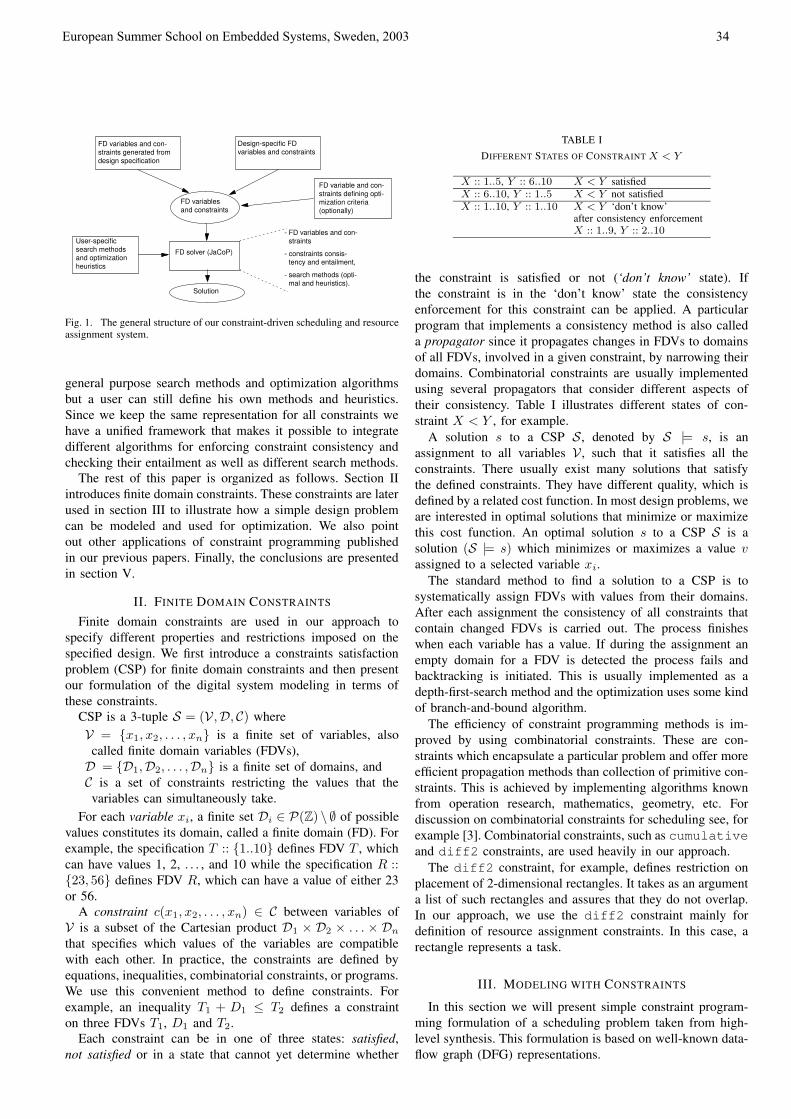
FD variablesand constraints
FD variables and con-straints generated fromdesign specification
Design-specific FDvariables and constraints
FD solver (JaCoP)
Solution
FD variable and con-straints defining opti-mization criteria(optionally)
- FD variables and con-straints
- constraints consis-tency and entailment,
- search methods (opti-mal and heuristics).
User-specificsearch methodsand optimizationheuristics
Fig. 1. The general structure of our constraint-driven scheduling and resourceassignment system.
general purpose search methods and optimization algorithmsbut a user can still define his own methods and heuristics.Since we keep the same representation for all constraints wehave a unified framework that makes it possible to integratedifferent algorithms for enforcing constraint consistency andchecking their entailment as well as different search methods.
The rest of this paper is organized as follows. Section IIintroduces finite domain constraints. These constraints are laterused in section III to illustrate how a simple design problemcan be modeled and used for optimization. We also pointout other applications of constraint programming publishedin our previous papers. Finally, the conclusions are presentedin section V.
II. FINITE DOMAIN CONSTRAINTS
Finite domain constraints are used in our approach tospecify different properties and restrictions imposed on thespecified design. We first introduce a constraints satisfactionproblem (CSP) for finite domain constraints and then presentour formulation of the digital system modeling in terms ofthese constraints.
CSP is a 3-tuple S = (V,D, C) whereV = x1, x2, . . . , xn is a finite set of variables, also
called finite domain variables (FDVs),D = D1,D2, . . . ,Dn is a finite set of domains, andC is a set of constraints restricting the values that the
variables can simultaneously take.For each variable xi, a finite set Di ∈ P(Z) \ ∅ of possible
values constitutes its domain, called a finite domain (FD). Forexample, the specification T :: 1..10 defines FDV T , whichcan have values 1, 2, . . . , and 10 while the specification R ::23, 56 defines FDV R, which can have a value of either 23or 56.
A constraint c(x1, x2, . . . , xn) ∈ C between variables ofV is a subset of the Cartesian product D1 × D2 × . . . × Dnthat specifies which values of the variables are compatiblewith each other. In practice, the constraints are defined byequations, inequalities, combinatorial constraints, or programs.We use this convenient method to define constraints. Forexample, an inequality T1 + D1 ≤ T2 defines a constrainton three FDVs T1, D1 and T2.
Each constraint can be in one of three states: satisfied,not satisfied or in a state that cannot yet determine whether
TABLE IDIFFERENT STATES OF CONSTRAINT X < Y
X :: 1..5, Y :: 6..10 X < Y satisfiedX :: 6..10, Y :: 1..5 X < Y not satisfiedX :: 1..10, Y :: 1..10 X < Y ‘don’t know’
after consistency enforcementX :: 1..9, Y :: 2..10
the constraint is satisfied or not (‘don’t know’ state). Ifthe constraint is in the ‘don’t know’ state the consistencyenforcement for this constraint can be applied. A particularprogram that implements a consistency method is also calleda propagator since it propagates changes in FDVs to domainsof all FDVs, involved in a given constraint, by narrowing theirdomains. Combinatorial constraints are usually implementedusing several propagators that consider different aspects oftheir consistency. Table I illustrates different states of con-straint X < Y , for example.
A solution s to a CSP S, denoted by S |= s, is anassignment to all variables V , such that it satisfies all theconstraints. There usually exist many solutions that satisfythe defined constraints. They have different quality, which isdefined by a related cost function. In most design problems, weare interested in optimal solutions that minimize or maximizethis cost function. An optimal solution s to a CSP S is asolution (S |= s) which minimizes or maximizes a value vassigned to a selected variable xi.
The standard method to find a solution to a CSP is tosystematically assign FDVs with values from their domains.After each assignment the consistency of all constraints thatcontain changed FDVs is carried out. The process finisheswhen each variable has a value. If during the assignment anempty domain for a FDV is detected the process fails andbacktracking is initiated. This is usually implemented as adepth-first-search method and the optimization uses some kindof branch-and-bound algorithm.
The efficiency of constraint programming methods is im-proved by using combinatorial constraints. These are con-straints which encapsulate a particular problem and offer moreefficient propagation methods than collection of primitive con-straints. This is achieved by implementing algorithms knownfrom operation research, mathematics, geometry, etc. Fordiscussion on combinatorial constraints for scheduling see, forexample [3]. Combinatorial constraints, such as cumulativeand diff2 constraints, are used heavily in our approach.
The diff2 constraint, for example, defines restriction onplacement of 2-dimensional rectangles. It takes as an argumenta list of such rectangles and assures that they do not overlap.In our approach, we use the diff2 constraint mainly fordefinition of resource assignment constraints. In this case, arectangle represents a task.
III. MODELING WITH CONSTRAINTS
In this section we will present simple constraint program-ming formulation of a scheduling problem taken from high-level synthesis. This formulation is based on well-known data-flow graph (DFG) representations.
European Summer School on Embedded Systems, Sweden, 2003
34

+ *
+
*
*+
-
*
+
+
(a) DFG
o1 o3o2Control
Step + *
+
*
*
+
1 3
4
5
8
10
-
*
+
+
2
6
7
9
1
2
3
4
6
5
(c) A generated schedule for 1 adder and 1 multiplier
T1+D1 ≤ T6, T6+D6 ≤ T9, T2+D2 ≤ T7,T3+D3 ≤ T8, T4+D4 ≤ T8, T8+D8 ≤ T10,T5+D5 ≤ T10,
for each ifor each j > i
(Ti+Di ≤ Tj ∨ Tj+Dj ≤ Ti ∨ Ri ≠ Rj)
o4 o5
o6 o7 o8
o9 o10
(b) Scheduling constraints
adder multiplier
Fig. 2. A simple data flow graph, scheduling constraints and its possibleschedule.
Assume that we have a set of partially ordered operations ortasks. We use the terms operation or task in a general sense.They represent an atomic computation such as addition ormultiplication in HLS or a specific algorithm such as discretecosine transform in system-level synthesis. The partial orderis usually represented using DFG as depicted in Figure III.a.
We first define FDVs specifically for this problem and laterdefine resource assignment and scheduling requirements asfinite domain constraints. For each operation, oi, we definethree FDVs, Ti, Di and Ri which represent the start timeof the operation, the operation’s delay and the resource usedfor its execution, respectively. Figure III.b depicts constraintsdefined for scheduling the DFG. First, operation precedenceconstraints for operations o1, o2, . . . , o10 are defined asinequalities. After that constraints on resource sharing aredefined. They prohibit resource sharing at the same controlstep and are defined using three disjunctive constraints foreach possible combination of operations.
A simple schedule for this example, which uses one adderand one multiplier (both with one clock delay), is depicted inFigure III.c. This schedule is found using a standard solvingmethod provided by constraint programming. This methodfinds a solution to the imposed constraint by systematicassignment of values to FDVs. Consistency of all constraints isenforced after each assignment. This prunes domains of FDVsand reduces the size of the search space. Combination of theFDVs assignment and branch-and-bound techniques providesstandard optimization method for constraint programming.
The example can be further improved by replacing alldisjunctive constraints constraints imposed in two for eachloops by single diff2 constraint [2].
IV. ADVANCED MODELING ISSUES
Various assumptions on tasks and scheduling methodscan produce different scheduling constraints. Our formulationmakes it possible to easily model multicycle operations, chain-ing or pipelined components in HLS. Algorithmic pipeliningcan also be modeled and solved efficiently [2].
HLS with conditional behaviors creates new challenges foroptimization. It is difficult since it introduces new optimizationopportunities by exploiting conditional resource sharing andspeculative execution. Our methods provide a way to modelmulticycle operations and chaining together with conditional
resource sharing and speculative execution. We can assignboth functional units and registers while making possible toconditionally share these components [4].
Register assignment traditionally requires careful analysissince registers can be shared between different variables.This assignment is decided based on the lifetime analysisof variables. The lifetime analysis, usually performed afterscheduling, determines a time interval when a variable isvalid and needs to occupy a register. In our approach, thelifetimes of variables can be modeled using rectangles (diff2constraint) that span on time axes during define-use time ofvariables [2]. This makes the modeling very easy and clear aswell as introduces opportunity to make scheduling and registerassignment simultaneously.
A solution of the imposed constraints provides a feasi-ble schedule which fulfills all requirements (i.e., imposedconstraints). Optimization can try to minimize different de-sign parameters, such as the number of time steps, cost ofused resources, power consumption, register/memory usageor a combination of these. In addition to standard constraintprogramming optimization methods, based on branch-and-bound principle, one can develop heuristic methods for specificdesign problems.
Constraint programming environment offers a flexible envi-ronment for solving different design problems. For example,it is possible to handle different scheduling problems whileproviding good performance. This is achieved mainly byefficient use of combinatorial constraints. These constraintsprovide efficient algorithms for narrowing domains of FDVs.More discussion on applying specific combinatorial schedulingand resource constraints for embedded system design problemscan be found in [2], [4]–[8].
Our approach has been evaluated using both commercialsolvers [9], [10] as well as a constraint programming li-brary developed specially for our purpose [2]. This con-straint programming library, called JaCoP (Java ConstraintProgramming environment), offers a set of constraints andsearch methods for problems found in embedded systemdesign.
Different extensions to model task graphs and related systemscheduling and assignment constraints has been studied andincluded in our formulation [8]. Our approach can handle thesedesign problems and offers new modeling opportunities. Forexample, constraint programming can be used for design spaceexploration and examination of different parameters, such asexecution time, cost, memory consumption, and energy (see,for example [11], [12]). In [13], an algorithm which examinesexecution time and energy consumption of a given application,while considering a parameterized memory architecture, ispresented. This algorithm produces Pareto trade-off pointsrepresenting different multi-objective execution options for thewhole application.
Constraints can be used to narrow design space by makingpartial decisions. This idea is exploited for task clusteringproblem and presented in [14]. Instead of clustering tasks, it isproposed to add additional constraints on task assignment andachieve reduction of design space. This approach can handlenon-linear clusters which traditional clustering cannot because
European Summer School on Embedded Systems, Sweden, 2003
35
of deadlock problems.
V. CONCLUSION
In this paper, we have briefly presented the method forembedded system modeling and design. Our method usesfinite domain constraints to model such systems and relatedconstraint solving techniques to find a final system imple-mentation. The presented approach makes it possible to mixdifferent types of constraints in a single model and usedifferent search methods as well as different optimizationtechniques. Both complete and heuristic search methods arepossible and therefore this approach is feasible in practice forlarge design problems that cannot be solved exactly. Optimalsolutions can be found when using complete search methodswhile the search space might be artificially cut for heuristicsearch techniques.
Our approach, based on CP techniques, for system modelingand design has several advantages that can be summarized asfollows:• Constraints can be used to formalize both a system model
and non-functional requirements of different types. Thefinal set of constraints specifies uniformly all require-ments on an implementation.
• A set of constraints can be easily extended with new con-straints to accommodate new requirements on a designwithout changing related synthesis algorithms.
• Different constraint solving techniques, heuristics andcomplete optimization methods, can be used to solve theconstraint model of the system.
• The use of constraints improves the general quality ofa design process by providing a way to control all con-straints in the same environment and assuring fulfillmentof all constraints.
• It provides a unifying framework for different constraintconsistency algorithms which, by narrowing domains offinite domain variables, contribute to a solution satisfyingall constraints.
The experimental results, published in different papers,prove usability of CP approach. It is competitive to both(M)ILP approaches and domain specific heuristics. It usuallycan provide good solutions in a reasonable time. On the other
hand CP offers possibility to incorporate well known heuris-tics. It is interesting approach since for the same model wecan use optimal methods, meta-heuristics or domain specificheuristics.
Concluding, the CP approach to embedded systems designprovides an attractive alternative to both domain specificheuristics and optimal methods based on (M)ILP.
REFERENCES
[1] K. Mariott and P. J. Stuckey, Programming with Constraints: AnIntroduction. The MIT Press, 1998.
[2] K. Kuchcinski, “Constraints-driven scheduling and resource assign-ment,” ACM Transactions on Design Automation of Electronic Systems(TODAES), vol. 8, no. 3, pp. 355–383, July 2003.
[3] P. Baptiste, C. Le Pape, and W. Nuijten, Constraint-Based Scheduling:Applying Constraint Programming to Scheduling Problems. KluwerAcademic Publisher, 2001.
[4] K. Kuchcinski and C. Wolinski, “Global approach to assignment andscheduling of complex behaviors based on HCDG and constraint pro-gramming,” Journal of Systems Architecture, vol. 49, no. 12–15, pp.489–503, 2003.
[5] K. Kuchcinski, “Embedded system synthesis by timing constraintssolving,” in Proc. 10th International Symposium on System Synthesis,Antwerp, Belgium, Sept. 17–19, 1997.
[6] F. Gruian and K. Kuchcinski, “Operation binding and scheduling for lowpower using constraint logic programming,” in Proc. 24th EuromicroConference, Workshop on Digital System Design, Vasteras, Sweden,August 25-27, 1998.
[7] R. Szymanek, F. Gruian, and K. Kuchcinski, “Digital systems designusing constraint logic programming,” in Proc. The Second InternationalConference on The Practical Applications of Constraint Logic Program-ming, (PACLP 2000), Manchester, UK, Apr. 10–12, 2000.
[8] K. Kuchcinski, “Constraints driven design space exploration for dis-tributed embedded systems,” Journal of Systems Architecture, vol. 47,no. 3-4, pp. 241–261, 2001.
[9] CHIP System Documentation, COSYTEC, 1996.[10] SICStus Prolog User’s Manual, Release 3.11.0, Swedish
Institute of Computer Science, Oct. 2003. [Online]. Available:http://www.sics.se/isl/sicstuswww/site/documentation.html
[11] R. Szymanek and K. Kuchcinski, “Task assignment and schedulingunder memory constraints,” in Proc. 26st Euromicro conference, Maas-tricht, The Netherlands, Sept. 5–7, 2000.
[12] ——, “A constructive algorithm for memory-aware task assignmentand scheduling,” in Proc. 9th International Symposium on Hard-ware/Software Codesign, Copenhagen, Denmark, Apr. 2001.
[13] R. Szymanek, F. Catthoor, and K. Kuchcinski, “Time-energy designspace exploration for multi-layer memory architectures,” in Proc. of 7thACM/IEEE Design, Automation and Test in Europe Conference, Paris,France, Feb. 16–20, 2004.
[14] R. Szymanek and K. Kuchcinski, “Partial task assignment of task graphsunder heterogeneous resource constraints,” in Proc. of the 40th DesignAutomation Conference, Anaheim, USA, June 2–6, 2003.
European Summer School on Embedded Systems, Sweden, 2003
36

European Summer School on Embedded Systems, Sweden, 2003
37
Embedded Systems Computer Architecture (Extended Abstract)
Jakob Engblom
Abstract—Embedded systems are computer systems used as
components in other systems. It is a very broad field encom-passing a large number of very different requirements, and the computer architecture of embedded systems reflects this variation by a large degree of specialization to application areas.
Index Terms— Embedded Systems, Computer Architecture
I. INTRODUCTION
Embedded systems are computer systems used as compo-nents in other systems. It is a very broad field encom-passing a large number of very different requirements,
and the computer architecture of embedded systems reflects this variation.
By their nature, embedded systems are special-purpose systems. In general, compared to a desktop or server machine, the computer employed in an embedded system will address a rather narrow, well-known, and fixed application. This makes it possible to specialize the computer architecture to address this particular application.
The performance demands of the system are usually well-defined at the design stage, and they are not likely to change over the lifetime of the system. This means that the performance and capabilities of an embedded system are targeted to the needs of the application. Extra performance or extra features over and above the particular needs of the application are a waste, not a feature. Sufficient performance is indeed sufficient. This is why billions of old 8-bit processors are still sold every year into the embedded market – for many tasks, they offer an acceptable solution.
There are three factors that need to be balanced to deter-mine the perfect computer base for an embedded system. The performance has to be sufficient. The cost has to be minimized. The power consumption (and heat production) has to be within design bounds. It is hard to satisfy all three goals simultaneously. Low power and low price also means low performance. Higher performance usually brings with it higher power consumption. Getting high performance cheap is always difficult. Sometimes, systems will need to be redesigned or specifications changed to accommodate the available processing power. Your mobile phone cannot currently have 3D graphics that can compete with a desktop PC, due to power and size constraints.
The best balance of power, performance, and cost is usually found in computer architectures specialized towards
a certain task. Barring a huge difference in production volumes, a general-purpose machine will always cost more and use more power than a special-purpose machine for the same problem. This is what gives the embedded systems space its unique diversity and room for innovation.
Manuscript received February 10, 2004. Jakob Engblom is a Business Development Manager at Virtutech
(http://www.virtutech.com) and an adjunct professor at Uppsala University, http://user.it.uu.se/~jakob. (e-mail: [email protected]).
One consequence of the attractiveness of specialized processing is that a system will often have multiple processors, each specializing in a particular type of task. A common distinction is between two styles of processing: control plane and data plane. The control plane is the part of a system that makes decisions and controls its behavior; it is usually dominated by decision making and data lookup. For example, in a telephone switch, this includes setting up the circuit for a phone call. The data plane, on the other hand, is the part of the system that is in charge of processing and shuffling data around; it is dominated by repetitive data movement and computations. In the phone switch example, this is the part that actually transports the sound stream from sender to receiver. Once the control plane has set up a call, the data plane will take over and do the work as long as the call is connected. This model, splitting control decisions and data is quite common, even though it obviously does not cover all embedded systems.
A final property of embedded systems that is often overlooked is the longevity of the systems. Many embedded systems, especially in the military and aerospace fields, have very long lifetimes, often reaching into decades. This makes future parts and tools availability a big issue in the design phase, as longevity has to be planned for.
II. EXAMPLES To give an idea for the wide span of systems that can be
called embedded, we will go through some examples. An advanced toy like the Lego Mindstorms robotics con-
struction kit contains a fairly simple processor: an 8-bit Hitachi H8 processor with 32k of ROM and 32k of RAM provides the brains for this quite sophisticated system. This offers a cheap and effective solution for creating a very fun smart toy.
A typical (non-smartphone) GSM phone contains a number of processors. An 8-bit processor might take care of the user interface, games, etc., while a 16-bit DSP provides the processing power necessary for digital voice encoding and decoding. Apart from these main processors, the Bluetooth unit in the phone contains an embedded 32-bit RISC processor used to process the communications protocol, as does the IR port. For smartphones that integrate more functions, 32-bit main processors are becoming necessary. So what we have is a small portable multiprocessor system.
Modern cars from manufacturers like Volvo, BMW, or Mercedes contain up to a hundred embedded processors.

European Summer School on Embedded Systems, Sweden, 2003
38
Some are powerful 32-bit processors used in engine control and similar compute-intensive tasks, while most are simpler 16-bit and 8-bit processors used to control various functions around the car (windows, locks, ACC, ABS brakes, etc.). The processors communicate with each other using buses like CAN, LIN, and FlexRay. Cars are extremely heterogeneous distributed systems. Since cost control is of essence for mass-production items like cars, each electronic unit is cost-minimized, even at the expense of a somewhat higher software development cost (since development costs are one-time expenses, while per-unit costs are incurred for each car produced). The processing power in cars is located where things need to happen; centralization is not an option.
Telephone systems contain a large number of embedded systems with varying computational needs and styles. For example, mobile phone base stations are computation-inten-sive digital signal processing systems. Such systems contain huge numbers of 32-bit or floating-point DSP processors to encode and decode radio signals and maintain the connections to the mobile phones. It is a very parallelizable system: each active phone requires the same processing of independent data, giving thousands of independent computation threads to spread across the DSP processors. They offer an almost perfect parallel workload. Several startups have tried to address this market with heavily parallel architectures.
Enterprise networking equipment like switches, routers and storage controllers make up another class of embedded systems. They are often quite similar to regular computers, containing one or a few 32-bit or 64-bit RISC processors, and running an operating system like Linux. However, the architecture is optimized to the movement of large amounts of data through the machine, using special line cards to take care of moving data while the main processor is only rarely involved. For the highest-capacity systems, custom CPU architectures are often employed, since regular processors are not well-suited to the task of packet processing.
Large military systems like radar stations and combat ships require enormous amounts of processing power, and here one can find regular multiprocessor servers working as embedded systems; albeit in special military-hardened cases. Even a Sun server can be considered an embedded system in the right circumstances! Often, military systems have tight space requirements, as ever more computing power is retrofitted to designs intended for far fewer computers.
Space-based systems offer another extreme: they need to employ special radiation-hardened cores and seldom enjoy the luxury of high clock frequencies or 32-bit processors.
III. THE MARKET Embedded processors make up about 98% of all
processors shipped (by number). Of about eight billion processors manufactured each year, only around 200 million find their way into desktops and servers. Looking at the overall semiconductor market, processors only make up about 2% of the numbers of parts sold, but about 30% of the revenue. So processors are clearly the highest margin part of the market to be in.
In the processor market, while 4-bit and 8-bit processors make up about 70% of the numbers, they only contribute a
tiny faction of the money. 32-bit and 64-bit processors (embedded or not) get more than 65% of the overall processor revenue, even though they are less than 10% of the numbers. Within the 32/64-bit category, desktops and servers takes almost all the money (50% of all processor revenue), thanks to the much higher price of server and desktop processors (usually hundreds of dollars apiece) compared to embedded processors (maybe tens of dollars, often less) [1].
So while embedded processors are dominant by numbers, we can see that it is very different on the revenue side. But 32-bit embedded processors are still a healthy and rapidly growing market that keeps attracting newcomers. ARM (www.arm.com), today’s most common 32-bit architecture, is produced in about 600 million units per year.
ARM is a good example of a business model peculiar to the embedded world, the licensable processor house. ARM designs processor cores and licenses them to other companies who then create products containing the ARM cores (combi-ning the core with various devices and memories to create sellable chip); ARM does not produce any chips of its own. This business model is also used by MIPS (www.mips.com), ARC (www.arc.com), Tensilica (www.tensilica.com), and others.
IV. PRODUCT CATEGORIES The embedded processor market defines itself around a
number of product categories, vaguely defined and featuring extensive overlap, but nevertheless they help organize and understand the market place.
A. Microprocessors The classic microprocessor is a chip that contains just a
processor, nowadays usually with integrated caches and sometimes memory controller. This is your SPARC, Pentium, and PowerPC processor found in regular office computers. Standalone processors are sometimes found in embedded systems, especially when lots of processing power is needed.
B. Microcontrollers A microcontroller is the traditional embedded processing
part. It encompasses not only the processor core, but also a number of peripheral devices like timers, serial ports, A/D converters, and network interfaces, along with some amount of program and data memory. The goal is to reduce the number of external chips needed, in order to minimize cost. Most microcontrollers are based on 8-bit or 16-bit processing cores, with a few kilobytes of data RAM and up to half a megabyte of ROM or FLASH memory for code. Typical microcontrollers are the Atmel AVR (www.atmel.com) and Microchip PIC (www.microchip.com) families.
C. ASIP/ASSP Recently, the term application-specific instruction set
processors (ASIP) or application-specific standard parts (ASSP) have come into use to denote “super-microcontrollers”. These chips take the level of integration on a single chip to new heights, based on the enormous number of transistors available in 130nm or smaller silicon processes. They are also “application-specific” in the sense that they are quite narrowly targeted to particular applications, and aim to
European Summer School on Embedded Systems, Sweden, 2003
39
replace the traditional development of custom hardware. Multiple cores and 32-bit processors are common in ASIP/ASSPs.
One good example are the Texas Instruments (www.ti.com) OMAP chips, which integrate an ARM core with a DSP core, memories, LCD and keyboard drivers, and other devices to put most of the logic of a mobile phone onto a single chip.
Infineon (www.infineon.com) has a family of chips built around the C167 core that are very popular in automotive applications. The C167 chips feature multiple on-chip CAN controllers, waveform generators, A/D and D/A converters, and many advanced timers.
Sometimes, ASIP/ASSP chips are billed as System-on-a-Chip (SoC) solutions. The term “SoC” has been getting very popular in recent years to denote highly-integrated chips that encompass all parts of a complete system, especially in the context of ASIC design (see below).
One particular class of ASIP/ASSPs are the network processing units (NPU). NPUs are chips designed specifically for networking applications, and include both control-plane and data-plane components. IBM’s (www.ibm.com) NP chips and Intel’s (www.intel.com) IPX are quite typical, combining a standard processor core with a large number of semi-programmable data pumps.
D. ASIC Application-Specific Integrated Circuits (ASICs), are the
ultimate embedded processing devices. ASICs are fully custom chips designed by the end user for the needs of a particular application. They can contain control logic, processing cores, memories, devices, buses, and whatever else an application might need.
Designing an ASIC is a very expensive process, and you will need large volumes or very special needs for it to be a viable proposition. As the number of gates that can be fit on a chip increases, ASIC design becomes ever more complex. The economics of ASICs are like classic printing: you have a high fixed setup cost to create the set of masks used to print the ASICs, but once the setup is done, the cost per unit is small. The more units you create, the lower the per-item cost will be.
One way to speed the design is to buy complex components from intellectual property (IP) providers. Most standard parts of an ASIC can be bought, from the simplest serial ports to processor cores. Processor cores (discussed briefly above) are the largest part of the IP business, since processors are the most complex part to design in-house (not to mention the need to create support tools like assemblers and compilers).
In some cases, ASICs include full-blown home-made special-purpose processors. A classic example is Ericsson’s (www.ericsson.com) APZ processor, used in the AXE series of digital phone switches. It is a very specialized architecture designed for the single application of phone switches. Another example is Cisco’s (www.cisco.com) Toaster series of switch processors; standard processors cannot process packets fast enough for high-end parts, so a special architecture was needed. None of these are available outside
the respective companies, making them ASICs and not microprocessors.
E. FPGAs Field-Programmable Gate Arrays, FPGAs, are “soft
hardware”. They are hardware chips whose function can be change by updating the contents of configuration memories. FPGAs are built from cells, small units implementing a small piece of logic controlled by configuration date. The cells are connected with a programmable interconnect to form complete circuits.
Compared to ASICs, FPGAs implement the same function in a much less efficient manner. Due to the obvious overhead in the implementation, FPGAs clock lower, exhibit higher power consumption, and contain fewer available logic gates. They also cost more per unit. But they are reprogrammable, and there is no setup cost like ASICs. This makes FPGAs more flexible and cheaper to design and work with.
FPGAs have always been popular as prototyping and validation tools: hardware designs can be validated by creating an FPGA and testing it, which is much faster and cheaper compared to creating a version of an ASIC.
In recent years, as costs for ASICs have increased drastically (startup costs are hitting millions of dollars for 130 nm and 90nm processes), FPGAs have become an alternative to ASICs in production units, especially for low-volume products. Currently, experts estimate that at volumes below hundreds of thousands of chips, FPGAs are more economical than ASICs. FPGAs also offer the possibility to fix bugs in the field by updating the FPGA programming.
Leaders in the FPGA field are Xilinx (www.xilinx.com) and Altera (www.altera.com). Since FPGAs (like all hardware logic) are best at parallel processing tasks with fixed functionality, some products combine regular processor cores with FPGA fabrics. The processor core takes care of unpredictable processing, while the FPGA part is used to accelerate processing suited to hardware implementation.
V. COMPUTER ARCHITECTURAL CHARACTERISTICS Embedded computer architecture is much more diverse
than general purpose desktop architectures. While it is to some extent true that technology trickles down from the PC/server market to embedded, there are many unique innovations occurring in the embedded market.
A. Instruction Sets One peculiarity of the embedded market is that old
architectures never die. Even in 2004, there will be billions of 8051s, Z80, and PIC chips sold: all 8-bit machines with instruction sets dating back to the 1970s. Also, the embedded market has given a second life to RISC architectures like MIPS that have faded from the general-purpose computer market. Furthermore, instruction set design goals and trade-offs are somewhat particular.
Code size is an important factor in most embedded designs, and instruction sets are designed and extended with code size in mind. Fairly typically, the NEC V850 (www.nec.com) architecture uses 16-, 32-, 48-bit, and 64-bit instructions to encode a RISC-style instruction set. The 32-bit ARM and
European Summer School on Embedded Systems, Sweden, 2003
40
MIPS architecture have been extended with reduced 16-bit instruction sets in order to reduce the code size. Instructions that perform a lot of work, like loading multiple values from the stack, are popular to reduce code size.
Instruction sets are also extended with instructions to accelerate particular processing tasks. For example, Motorola’s (www.motorola.com) 68300 processors have a special table lookup and interpolate instruction to accelerate engine control tasks.
Of particular note are the DSP (Digital Signal Processing) instruction sets. DSP processors are specialized to performing data-plane processing, designed to take advantage of the regular structure of most interesting program loops, and with special instructions for common tasks (for example, FIR filters can be implemented with a single instruction on a TI C65).
The most extreme example of application-adapted instructtion sets are offered by the configurable processors. Tensilica and Arc are the leaders in this field, where processor cores are customized by selecting which particular instructions to include in a particular configuration. It is also possible for the user to create new instructions to accelerate particular tasks.
B. Memory Systems Embedded systems often feature quite complex memory
systems. Caches are normally quite simple, featuring single-level instruction and data caches. However, the caches are often complemented with tightly-coupled memories (TCM), fast on-chip memories that are under programmer control and not automatically managed by the cache system. Compared to caches, TCMs are more predictable (good for real-time systems) and use less power (thanks to reduced complexity). For IP cores, the size of caches and TCMs is usually configurable.
Memory is preferably kept on-chip to reduce power consumption and product cost: adding external memory chips is fairly expensive both in terms of production cost and power consumption. Usually, code is kept in ROM or FLASH memory on-chip, with a much smaller RAM memory for storage of variables and stacks (most embedded systems follow the classic “Harvard” design of separating code and data physically). EEPROM or FLASH memory is used to keep persistent data when the system is powered off. High-end systems require off-chip memories: even today, it is hard to fit more than a few megabytes of memory on-chip.
On 8-bit and 16-bit architectures, pointers are limited in size. To accommodate larger memories, there is usually a hierarchy of memory areas and pointer types. There might be a zero-page memory which is addressed using an 8-bit pointer, with a “near” memory with 16-bit pointers, and various forms of “far” memory with 24- or 32-bit pointers. This leads to a programming model where the programmer needs to be aware of the allocation of variables to memory in order to efficient programs.
C. Pipelines Pipelines in embedded processors tend to be simpler than
their desktop counterparts, since the goal is to provide ade-quate performance with minimal cost and power consump-
tion. For example, the ARM926 core requires up to 0.9 mW/Mhz; while the Pentium 4 uses about 35 mW/Mhz. The cost to go from acceptable to maximum performance can be very high!
8-bit and 16-bit processors are usually not pipelined at all, while 32-bit processors use everything from the simple 3-stage pipeline of the ARM7 to complex multiple-issue out-of-order pipelines on 64-bit MIPS systems. Currently, most 32-bit machines have moderately complex pipelines with 5 to 7 stages and strict in-order issue. Every generation of embedded processor cores tend to add a few more features in order to add processing power, but it is always done within the constraints posed by cost, size, and power consumption.
Since the tasks requiring the most processing power are usually well-known, they can be more efficiently solved by using hardware accelerators or special processors instead of a faster general-purpose processor. This leads to the classic RISC-DSP split of processing in mobile phones, and the use of special acceleration hardware for tasks like MPEG decoding.
There are also some truly extreme designs in the embedded field. Xelerated’s (www.xelerated.com) network processors use a pipeline more than 1000 stages deep to efficiently rout and filter network packets. Texas Instruments are successfully selling eight-wide VLIW DSP processors for customers requiring very high performance signal processing.
VI. SUMMARY This talk has given a quick overview of the embedded
computer architecture field. I have tried to give a feeling for the broadness of the embedded systems field and the wide range of particular computer designs that have been created to correspond to the many peculiar needs of the various end-user applications.
The main fact to remember is this: there is no typical embedded system, and any computer architecture feature ever invented is bound to have a valid application somewhere in the embedded systems field.
REFERENCES [1] Jim Turley, “The Two Percent Solution”, Embedded.com, Dec 18,
2002. http://www.embedded.com/story/OEG20021217S0039
Compilation for Embedded ProcessorsDaniel Kastner
AbsInt Angewandte Informatik GmbHSaarbr¨ucken, Germany
Abstract— This article gives an overview of the field of compi-lation for embedded processors. First, typical characterisitics ofembedded processors are summarized that have to be taken intoaccount in order to generate high-quality machine code. A lectureconcept is outlined which starts by introducing the necessary ba-sics of compiler technology, then details the specific requirementsof compilation for embedded processors and concludes with anoverview of recent research in this field. The lecture was heldin the Embedded Systems Schummer School ESSES 2003. Thearticle concludes with a literature survey that can serve as astarting point for further research in this area.
Index Terms— Compilation, Code Generation, Embedded Pro-cessors, Retargetability, Code Compaction, Postpass Optimiza-tion.
I. I NTRODUCTION
EMBEDDED systems are increasingly becoming a fixedpart of everyday’s life. Already today, the vast majority
of all microprocessors sold are used in embedded systems;application fields comprise healthcare technology, telecom-munication, automotive and avionics, multimedia applications,etc. The main requirement imposed to embedded systems ishigh efficiency: high performance must come at low cost andat low power consumption. This has led to the developmentof irregular hardware architectures specially designed for real-time applications and digital signal processing.
The architectural irregularity of many embedded processorsimposes new challenges to the code generation task. In thearea of the classical general-purpose processors, compilertechnology has reached a high level of maturity. However, forirregular architectures, the code quality achieved by traditionalhigh-level language compilers is often far from satisfactory[1], [2]. Generating efficient code for irregular architecturesrequires highly optimizing techniques that have to be awareof specific hardware features of the target processor. The codegeneration process can be subdivided into several subtasksmost of which are NP-complete problems: code selection,register allocation, instruction scheduling, register assignmentand functional unit binding. In classical approaches they areaddressed in separate phases by heuristic algorithms. Sincethese phases are interdependent, decisions made in one phaseimpose constraints to the subsequently addressed phases. Thiscan lead to a suboptimal combination of suboptimal partialsolutions resulting in a very poor code quality – especiallyfor irregular architectures [1]. The shortcomings of availablecompilers have resulted in many embedded applications beingdeveloped in assembly language, or at least in part. Here,search-based techniques allowing to model the interactionsof code generation phases in an exact way, or combinations
of search-based techniques with standard heuristic approachescan lead to substantially better code quality [3], [4].
Due to the growing complexity of embedded applicationsand the shrinking design cycles of embedded products theusage of high-level programming languages is becoming in-creasingly imperative. Thus there is an urgent need forretar-getablecode generation and optimization techniques that canbe quickly adapted to different target architectures, e.g. by de-riving machine-specific properties from a dedicated hardwaredescription. At the same time these techniques must be ableto produce high-quality code for the modeled architectures.
Many of today’s microprocessors use instruction-level par-allelism to achieve high performance. They typically havemultiple execution units and provide multiple issue slots(EPIC, VLIW) or deep pipelining (superscalar architectures).However, since the amount of parallelism inherent in programstends to be small [5], it is a problem to keep the availableexecution units busy. For architectures with static instruction-level parallelism this problem is especially virulent, sinceif not enough parallelism is available the issue slots of thelong instruction words are filled with nops. For embeddedprocessors this means a waste of program memory and energy.Techniques to exploit the available instruction-level paral-lelism play an important role in compilation for embeddedprocessors.
While the traditional metrics for compiler quality wasthe execution speed of the generated code, the mass scaleembedded market has caused two other metrics to come toimportance: code size and power consumption. One of themost dominant factors in system cost is the die size, inwhich memory plays an important role. Reducing memoryconsumption directly translates to reducing system cost and, atthe same time, to lowering power consumption. For efficientlyreducing code size cross-file optimizations are required [6]which can eliminate redundancies and unused functionalityover entire applications. At the same time, they must be ableto take advantage of individual hardware characteristics of thetarget processor.
To summarize, in order to generate efficient code forembedded processors, the following challenges have to bemet: exploiting the available instruction-level parallelism ofthe target processor, efficiently modeling irregular hardwarerestrictions during code generation, addressing the phase-coupling problem, achieving retargetability, and supportingsmall code size and low power consumption as alternative codegeneration goals.
In the follwing, a lecture concept is described which tries toimpart the basics of compiler technology required to grasp the
European Summer School on Embedded Systems, Sweden, 2003
41

specifics of embedded compilation and also addresses recentresearch in this field. The lecture was held in the EmbeddedSystems Schummer School ESSES 2003 with a time frame ofsix hours ([?]).
II. A L ECTURE ONEMBEDDED COMPILATION
The lecture is introduced by an overview of the struc-ture of an optimizing compiler is given. The compiler frontend transforms the high-level language input program in anintermediate representation suitable for code generation. Itconsists of the phases lexical analysis, syntactical analysisand semantic analysis. The middle end performs efficiency-increasing transformations of the intermediate representation,often erroneously termedmachine-independent optimizations.The compiler backend is concerned with generating the ma-chine code for the target processor. Code generation phasesare code selection, register allocation, instruction schedulingand functional unit binding. The phase coupling problem isthe result of the inderdependences between all these phaseswhich mostly are NP-complete problems by themselves.
The second part of the lecture addresses the specific codegeneration problem for embedded processors and explainsthe motivation for the development of specialized hardwarearchitectures.
Program representations play an important role in codegeneration. Many compiler phases look at the input programfrom different views, each of which usually is mapped toa representation of its own. An important concept is todistinguish between high-level intermediate representationsdescribing the input program from a view close to sourcelevel, and the low-level representations used to incorporatemachine-specific characteristics. The most prominent programrepresentations are syntax trees, (inter-procedural) control flowgraphs, control dependence graphs, data dependence graphs,register interference graphs and the SSA form.
The discussion of program representations is followed by abrief overview of standard code generation techniques. Reg-ister allocation usually is done by graph coloring algorithms.Instruction scheduling techniques can be classified as localacyclic vs. global acyclic vs. global cyclic approaches. Thelecture focuses on list scheduling as a standard local acyclictechnique, on trace scheduling and superblock scheduling asglobal acyclic approaches. The task of code selection canbe described by regular tree automata accepting words ofregular tree grammars. From this theory, generating a codeselector can be formalized as generating a tree automaton forthe underlying machine grammar. Examples of current codeselector generators are given.
The next part focuses on retargetable compilation. Theterm retargetability is explained, and an overview of currentresearch on retargetability is given. As an example of aretargetable code generation system the PROPAN framework[3], [4] is presented. At the heart of each retargetable systemthere is an underlying architecture description language. Archi-tecture description languages can be categorized as structural,behavioral, or mixed-level languages. The design philosophiesof these different classes are explained, and the hardware de-
scription language of the PROPAN system, TDL, is presentedas an example.
In the remainder of the lecture, advanced code generationtopics are addressed. The basic idea of software pipelining asthe most prominent cyclic scheduling technique is explainedusing iterative modulo scheduling as example algorithm. Sub-sequently, an algorithm to exploit SIMD-style instructionsis presented where long registers are loaded with multipleshort data values which are simultaneously operated on [31].Phase coupling problems exist between code selection andregister allocation, code selection and instruction scheduling,as well as between register allocation and instruction schedul-ing. Examples for each scenario are given, and integer pro-gramming techniques are presented which address the phase-coupling problem between instruction scheduling and registerassignment. The importance of code size as alternative qualitymetrics is illustrated by an industrial case study: a demo ofthe commercial postpass optimizer aiPop [55] is given andits structure and algorithms are explained. The last part of thelecture is concerned with program analyses as a prerequisite ofmost compiler transformations and as stand-alone applications,e.g. , to give static runtime guarantees for real-time systems.
III. L ITERATURE OVERVIEW
In the following an overview of relevant literature for thedifferent topics is given. This survey in no way is complete;it is intended to offer a starting point for further research inthe area of embedded compilation.
A. Compiler Design
Text books about compiler construction providing a compre-hensive survey of the field are [7], [8], [9], [10]. Publicationsfocusing on the different backend phases are summarized inthe following.
1) Code Selection:The basic idea of code selector gen-erators can be formalised by the theory of tree parsing andtree automata [11], [8]. The instruction set of the targetmachine is described by a regular tree grammar. The derivationtree of an expression tree describes a semantically equivalentsequence of machine operations. Cost annotations to the gram-mar rules permit to locally select a cheapest derivation tree.Early implementations based on [12], [13] used LR-parsingtechniques driven by a specification of the target machine bya context-free grammar. The code selector was generated bya parser generator. The limitation was that the code selectionfor ambiguous instruction sets could not be modelled con-veniently. A solution of this problem is to combine patternmatching algorithms with dynamic programming to determinelocally optimal operation sequences [14], [15] or extend thepattern matcher to directly selecting locally optimal operationsequences [16]. Examples for contemporary code generatorsare BEG [17], Twig [18], iburg [19], and OLIVE [20].
2) Register Allocation:Typically, register allocation is per-formed by graph colouring algorithms. Selecting registers ismapped to the problem of finding a coloring in the so-called register interference graph. Since for this isan NP-complete problem, usually registers are allocated in a
European Summer School on Embedded Systems, Sweden, 2003
42
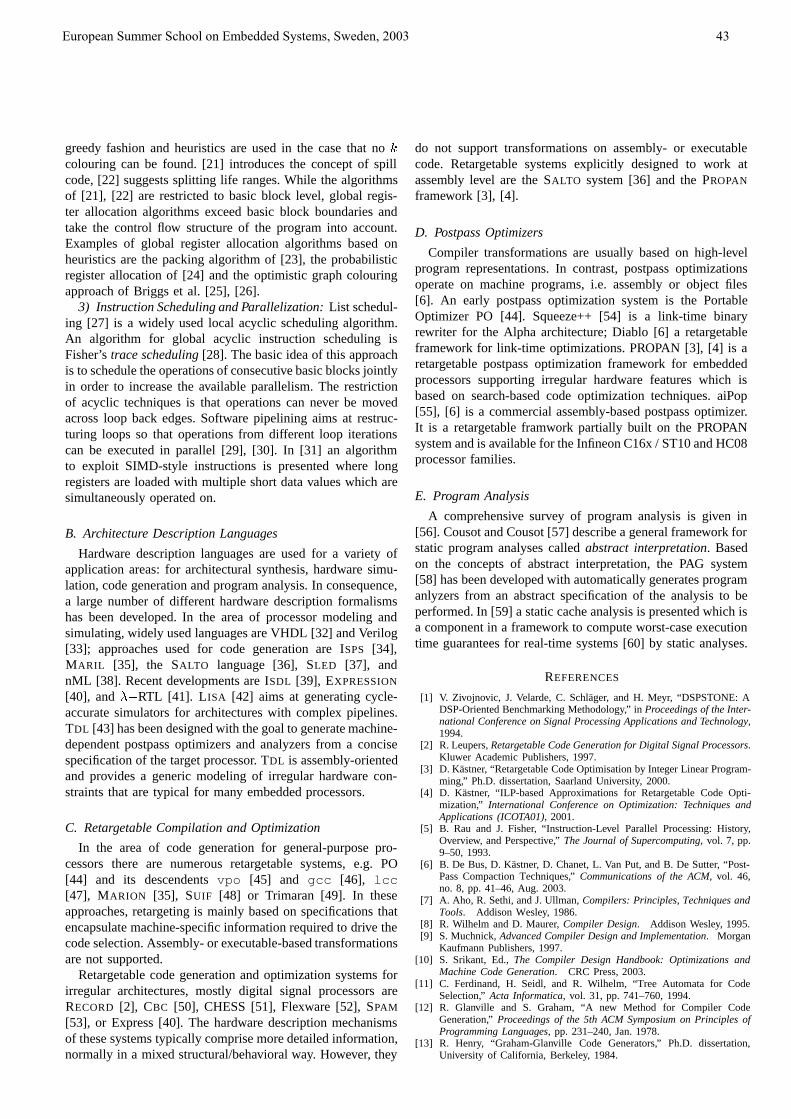
greedy fashion and heuristics are used in the case that no
colouring can be found. [21] introduces the concept of spillcode, [22] suggests splitting life ranges. While the algorithmsof [21], [22] are restricted to basic block level, global regis-ter allocation algorithms exceed basic block boundaries andtake the control flow structure of the program into account.Examples of global register allocation algorithms based onheuristics are the packing algorithm of [23], the probabilisticregister allocation of [24] and the optimistic graph colouringapproach of Briggs et al. [25], [26].
3) Instruction Scheduling and Parallelization:List schedul-ing [27] is a widely used local acyclic scheduling algorithm.An algorithm for global acyclic instruction scheduling isFisher’strace scheduling[28]. The basic idea of this approachis to schedule the operations of consecutive basic blocks jointlyin order to increase the available parallelism. The restrictionof acyclic techniques is that operations can never be movedacross loop back edges. Software pipelining aims at restruc-turing loops so that operations from different loop iterationscan be executed in parallel [29], [30]. In [31] an algorithmto exploit SIMD-style instructions is presented where longregisters are loaded with multiple short data values which aresimultaneously operated on.
B. Architecture Description Languages
Hardware description languages are used for a variety ofapplication areas: for architectural synthesis, hardware simu-lation, code generation and program analysis. In consequence,a large number of different hardware description formalismshas been developed. In the area of processor modeling andsimulating, widely used languages are VHDL [32] and Verilog[33]; approaches used for code generation are ISPS [34],MARIL [35], the SALTO language [36], SLED [37], andnML [38]. Recent developments are ISDL [39], EXPRESSION
[40], andRTL [41]. LISA [42] aims at generating cycle-accurate simulators for architectures with complex pipelines.TDL [43] has been designed with the goal to generate machine-dependent postpass optimizers and analyzers from a concisespecification of the target processor. TDL is assembly-orientedand provides a generic modeling of irregular hardware con-straints that are typical for many embedded processors.
C. Retargetable Compilation and Optimization
In the area of code generation for general-purpose pro-cessors there are numerous retargetable systems, e.g. PO[44] and its descendentsvpo [45] and gcc [46], lcc[47], MARION [35], SUIF [48] or Trimaran [49]. In theseapproaches, retargeting is mainly based on specifications thatencapsulate machine-specific information required to drive thecode selection. Assembly- or executable-based transformationsare not supported.
Retargetable code generation and optimization systems forirregular architectures, mostly digital signal processors areRECORD [2], CBC [50], CHESS [51], Flexware [52], SPAM
[53], or Express [40]. The hardware description mechanismsof these systems typically comprise more detailed information,normally in a mixed structural/behavioral way. However, they
do not support transformations on assembly- or executablecode. Retargetable systems explicitly designed to work atassembly level are the SALTO system [36] and the PROPAN
framework [3], [4].
D. Postpass Optimizers
Compiler transformations are usually based on high-levelprogram representations. In contrast, postpass optimizationsoperate on machine programs, i.e. assembly or object files[6]. An early postpass optimization system is the PortableOptimizer PO [44]. Squeeze++ [54] is a link-time binaryrewriter for the Alpha architecture; Diablo [6] a retargetableframework for link-time optimizations. PROPAN [3], [4] is aretargetable postpass optimization framework for embeddedprocessors supporting irregular hardware features which isbased on search-based code optimization techniques. aiPop[55], [6] is a commercial assembly-based postpass optimizer.It is a retargetable framwork partially built on the PROPANsystem and is available for the Infineon C16x / ST10 and HC08processor families.
E. Program Analysis
A comprehensive survey of program analysis is given in[56]. Cousot and Cousot [57] describe a general framework forstatic program analyses calledabstract interpretation. Basedon the concepts of abstract interpretation, the PAG system[58] has been developed with automatically generates programanlyzers from an abstract specification of the analysis to beperformed. In [59] a static cache analysis is presented which isa component in a framework to compute worst-case executiontime guarantees for real-time systems [60] by static analyses.
REFERENCES
[1] V. Zivojnovic, J. Velarde, C. Schl¨ager, and H. Meyr, “DSPSTONE: ADSP-Oriented Benchmarking Methodology,” inProceedings of the Inter-national Conference on Signal Processing Applications and Technology,1994.
[2] R. Leupers,Retargetable Code Generation for Digital Signal Processors.Kluwer Academic Publishers, 1997.
[3] D. Kastner, “Retargetable Code Optimisation by Integer Linear Program-ming,” Ph.D. dissertation, Saarland University, 2000.
[4] D. Kastner, “ILP-based Approximations for Retargetable Code Opti-mization,” International Conference on Optimization: Techniques andApplications (ICOTA01), 2001.
[5] B. Rau and J. Fisher, “Instruction-Level Parallel Processing: History,Overview, and Perspective,”The Journal of Supercomputing, vol. 7, pp.9–50, 1993.
[6] B. De Bus, D. Kastner, D. Chanet, L. Van Put, and B. De Sutter, “Post-Pass Compaction Techniques,”Communications of the ACM, vol. 46,no. 8, pp. 41–46, Aug. 2003.
[7] A. Aho, R. Sethi, and J. Ullman,Compilers: Principles, Techniques andTools. Addison Wesley, 1986.
[8] R. Wilhelm and D. Maurer,Compiler Design. Addison Wesley, 1995.[9] S. Muchnick,Advanced Compiler Design and Implementation. Morgan
Kaufmann Publishers, 1997.[10] S. Srikant, Ed.,The Compiler Design Handbook: Optimizations and
Machine Code Generation. CRC Press, 2003.[11] C. Ferdinand, H. Seidl, and R. Wilhelm, “Tree Automata for Code
Selection,”Acta Informatica, vol. 31, pp. 741–760, 1994.[12] R. Glanville and S. Graham, “A new Method for Compiler Code
Generation,”Proceedings of the 5th ACM Symposium on Principles ofProgramming Languages, pp. 231–240, Jan. 1978.
[13] R. Henry, “Graham-Glanville Code Generators,” Ph.D. dissertation,University of California, Berkeley, 1984.
European Summer School on Embedded Systems, Sweden, 2003
43

[14] A. Aho and M. Ganapathi, “Efficient Tree Pattern Matching: An Aidto Code Generation,”Proceedings of the 12th ACM Symposium onPrinciples of Programming Languages, pp. 334–340, 1985.
[15] B. Weisgerber and R. Wilhelm, “Two Tree Pattern Matchers for CodeSelection (Including Targeting),” inCompiler Compilers and High SpeedCompilation, D. Hammer, Ed. Springer LNCS 371, 1989, pp. 215–229.
[16] E. Pelegri-Llopart and S. Graham, “Optimal Code Generation forExpression Trees: An Application of BURS Theory,”Proceedings ofthe 15th ACM Symposium on Principles of Programming Languages,pp. 294–308, 1988.
[17] H. Emmelmann,BEG – a Back End Generator, GMD Forschungsstellean der Universit¨at Karlsruhe, Nov. 1989.
[18] A. Aho, M. Ganapathi, and S. Tjiang, “Code Generation Using TreeMatching and Dynamic Programming,”ACM Transactions on Program-ming Languages and Systems, vol. 11, no. 4, pp. 491–516, Oct. 1989.
[19] C. Fraser, D. Hanson, and T. Proebsting, “Engineering a Simple,Efficient Code-Generator Generator,”ACM Letters on ProgrammingLanguages and Systems, vol. 1, no. 3, pp. 213–226, 1992.
[20] SPAM Compiler User’s Manual, SPAM Research Group,http://www.ee.princeton.edu/spam, Sept. 1997.
[21] G. Chaitin, “Register Allocation and Spilling via Graph Coloring,” inProc. SIGPLAN’82 Symp. on Compiler Construction, SIGPLAN Notices,vol. 17(6), 1982, pp. 201–207.
[22] F. Chow and J. Hennessy, “The Priority-Based Coloring Approach toRegister Allocation,”ACM Transactions on Programming Languagesand Systems, vol. 12, no. 4, pp. 501–536, 1990.
[23] M. Benitez, “Register Allocation and Phase Interactions in RetargetableOptimizing Compilers,” Ph.D. dissertation, University of Virginia, May1994.
[24] T. Proebsting and C. Fisher, “Probabilistic Register Allocation,” inProceedings of the ACM SIGPLAN 1992 Conference on ProgrammingLanguage Design and Implementation, Jan. 1992, pp. 300–310.
[25] P. Briggs, “Register Allocation via Graph Coloring,” Ph.D. dissertation,Rice University, Houston, Texas, Apr. 1992.
[26] P. Briggs, K. Cooper, and L. Torczon, “Improvements to Graph ColoringRegister Allocation,”ACM Transactions on Programming Languagesand Systems, vol. 16, no. 3, pp. 428–455, 1994.
[27] D. Landskov, S. Davidson, and B. Shriver, “Local Microcode Com-paction Techniques,”ACM Computing Surveys, vol. 12, no. 3, pp. 261–294, Sept. 1980.
[28] J. Fisher, “Trace Scheduling: A Technique for Global Microcode Com-paction,” IEEE Transactions on Computers, vol. C-30, no. 7, pp. 478–490, July 1981.
[29] V. Allan, R. Jones, R. Lee, and S. Allan, “Software Pipelining,”Computing Surveys, vol. 27, no. 3, pp. 367–432, Sept. 1995.
[30] B. Rau, “Iterative Modulo Scheduling,”International Journal of ParallelProcessing, vol. 24, 1996.
[31] S. Larsen and S. Amarasinghe, “Exploiting Superword Level Parallelismwith Multimedia Instruction Sets,”ACM SIGPLAN Notices, 2000.
[32] R. Lipsett, C. Schaefer, and C. Ussery,VHDL: Hardware Descriptionand Design, 12nd ed. Kluwer Academic Publishers, 1993.
[33] D. Thomas and P. Moorby,The Verilog Hardware Description Language,2nd ed. Kluwer Academic Publishers, 1995.
[34] M. Barbacci, “Instruction Set Processor Specifications (ISPS): TheNotation and Its Applications,”IEEE Transactions on Computers, vol.C-30, no. 1, pp. 24–40, Jan. 1981.
[35] D. Bradlee, R. Henry, and S. Eggers, “The Marion System for Retar-getable Instruction Scheduling,”Proceedings of the PLDI, pp. 229–240,1991.
[36] F. Bodin, Z. Chamski, E. Rohou, and A. Seznec,Functional Spe-cification of SALTO: A Retargetable System for Assembly LanguageTransformation and Optimization, rev. 1.00 beta, INRIA, 1997.
[37] N. Ramsey and M. Fernandez, “Specifying Representations of MachineInstructions,”ACM Transactions on Programming Languages and Sys-tems, vol. 19, no. 3, pp. 492–524, May 1997.
[38] A. Fauth, J. Van Praet, and M. Freericks, “Describing Instruction SetProcessors Using nML,” inProceedings of the European Design andTest Conference. IEEE, 1995, pp. 503–507.
[39] G. Hadjiyiannis, “ISDL: Instruction Set Description Language Version1.0,” MIT RLE, Tech. Rep., Apr. 1998.
[40] A. Halambi, P. Grun, V. Ganesh, A. Khare, N. Dutt, and A. Nicolau,“EXPRESSION: A Language for Architecture Exploration throughCompiler/Simulator Retargetability,”Proceedings of the DATE99, 1999.
[41] J. Davidson and N. Ramsey, “Machine Descriptions to Build Tools forEmbedded Systems,” inProceedings of the ACM SIGPLAN Workshopon Languages, Compilers and Tools for Embedded Systems. SpringerLNCS, Volume 1474, June 1998, pp. 172–188.
[42] S. Pees, A. Hoffmann, V. Zivojnovic, and H. Meyr, “LISA: MachineDescription Language for Cycle-Accurate Models of ProgrammableDSP Architectures,”Proceedings of the Design Automation Conference,1999.
[43] D. Kastner, “TDL: A Hardware Description Language for RetargetablePostpass Optimizations and Analyses,” inProceedings of the ACMSIGPLAN/SIGSOFT Conference on Generative Programming and Com-ponent Engineering (GPCE03), 2003.
[44] J. Davidson and C. Fraser, “Code Selection through Object Code Opti-mization,” ACM Transactions on Programming Languages and Systems,vol. 6, no. 4, pp. 505–526, Oct. 1984.
[45] M. Benitez and J. Davidson, “Target-Specific Global Code Improve-ment: Principles and Applications,” Department of Computer Science,University of Virginia, Charlottesville, Tech. Rep., 1994.
[46] R. Stallman,Using and Porting GNU CC, Free Software Foundation,Cambridge/Massachusetts, 1998.
[47] C. Fraser and D. Hanson,A Retargetable C Compiler: Design AndImplementation. Benjamin/Cummings Publishing Company, Inc., 1995.
[48] SUIF Compiler System: The SUIF Library, Stanford Compiler Group,1994.
[49] “TRIMARAN: An Infrastructure for Research in Instruction-Level Par-allelism,” http://www.trimaran.org.
[50] A. Fauth, “Beyond Tool-Specific Machine Descriptions,” in[61] .Kluwer, 1995, ch. 8, pp. 138–152.
[51] D. Lanneer, J. Van Praet, A. Kifli, K. Schoofs, W. Geurts, F. Thoen, andG. Goossens, “CHESS: Retargetable Code Generation For EmbeddedDSP Processors,” in[61] . Kluwer, 1995, pp. 85–102.
[52] P. Paulin, C. Liem, T. May, and S. Sutarwala, “FLEXWARE: A FlexibleFirmware Development Environment for Embedded Systems,” in[61] .Kluwer, 1995, pp. 67–84.
[53] A. Sudarsanam, “Code Optimization Libraries for Retargetable Com-pilation for Embedded Digital Signal Processors,” Ph.D. dissertation,University of Princeton, Nov. 1998.
[54] S. Debray, W. Evans, R. Muth, and B. De Sutter, “Compiler Techniquesfor Code Compaction,”ACM Transactions on Programming Languagesand Systems, vol. 22, no. 2, pp. 378–415, 2000.
[55] C. Ferdinand, “Post Pass Code Compaction at the Assembly Level forthe C16x,”Contact Magazine, Sept. 2000.
[56] F. Nielson, H. Nielson, and C. Hankin,Principles of Program Analysis.Springer, 1999.
[57] P. Cousot and R. Cousot, “Abstract Interpretation: A Unified LatticeModel for Static Analysis of Programs by Construction or Approxi-mation of Fixpoints,” in4th POPL, Los Angeles, CA, Jan. 1977, pp.238–252.
[58] F. Martin, “Generation of Program Analyzers,” Ph.D. dissertation, Saar-land University, 1999.
[59] C. Ferdinand, “Cache behavior prediction for real-time systems,” Ph.D.dissertation, Saarland University, 1997.
[60] C. Ferdinand, R. Heckmann, M. Langenbach, F. Martin, M. Schmidt,H. Theiling, S. Thesing, and R. Wilhelm, “Reliable and Precise WCETDetermination for a Real-Life Processor,” inEMSOFT, LNCS 2211.Springer, 2001, pp. 469–485.
[61] P. Marwedel and G. Goossens,Code Generation for Embedded Proces-sors. Boston; London; Dortrecht: Kluwer, 1995.
Daniel Kastner Born 1973, he studied computerscience and business economics at Saarland Univer-sity, Germany, from 1993 to 1997. He received theVDI Saar 1998 award for the best diploma thesis incomputer science at Saarland University. In 2000,he finished his Ph.D. on “Retargetable PostpassOptimisation by Integer Linear Programming” whichwas awarded the “SaarLB Science Award” 2003. Inhis Ph.D thesis he developed a retargetable systemfor phase-coupled code optimization at the assemblylevel, which is able to take advantage of irregular
hardware features commonly found in embedded processors.Daniel Kastner is a co-founder of the company AbsInt GmbH which
focuses on compiler technology, especially on program analyses and programoptimizations for embedded systems. His scientific work is centered aroundcode generation and optimization techniques, dynamic compilation, integerprogramming, language design, microprocessor modeling, embedded systems,java virtual machines and task scheduling for real-time systems.
European Summer School on Embedded Systems, Sweden, 2003
44

European Summer School on Embedded Systems, Sweden, 2003
45
Full-System Simulation (Extended Abstract)
Jakob Engblom
Abstract—Full-System Simulation is a technology where the
hardware of a computer system is simulated at such a level of detail that the complete real software stack can be executed. It has wide applicability in the development and research of computer systems, especially embedded systems. This talk gives an overview of the full-system simulation and some examples of its industrial and academic applications.
I. INTRODUCTION
SIMULATION is a method of scientific and engineering inquiry that is based on the idea of building a model of a
system, and then performing experiments on this model. Provided that the model has a good fidelity to the system being modeled, the results from the simulation experiments can be used to predict the behavior of the real system.
Simulation is used in all fields of science and engineering. For example, modern cars are virtually crash tested in computer simulation in order to build safer cars. Weather forecasts are prepared by simulating the evolution of current weather patterns into the future.
Computers can also be used to simulate computer systems. This introspective application of computers is incredibly useful, across all fields of computer hardware and software development, from initial architecture, through software development, to end-of-life maintenance.
A key concept is full-system simulation, meaning models that encompass all of a computer system. Including the processor core, its peripheral devices, memories, and network connections. With such technology, it is possible to simulate a whole computer system with its complete software stack, which opens up new possibilities in the field of computer-system simulation [1][2][3][4].
Full-system simulation has not been feasible until recently, thanks to two long-term technology trends. One is the fact that cheap PCs have become as fast as any other computer system; it used to be that in order to simulate a large server you needed a large server, but this is no longer the case [2]. The other trend is that simulation technology has improved the efficiency of simulation by orders of magnitude. The net result is that the simulation cost per hour of target time has come down by four orders of magnitude over the past 25 years [1]!
II. FULL-SYSTEM SIMULATION The idea behind full-system simulation is very simple:
model the behavior of the hardware of a system at a sufficient level of detail that all the real software can run (Figure 1); at a level of abstraction appropriate to simulating complete systems containing multiple processors and machines, potentially connected across simulated networks.
Manuscript received January 31, 2004. Jakob Engblom is a Business Development Manager at Virtutech
(http://www.virtutech.com) and an adjunct professor at Uppsala University (http://user.it.uu.se/~jakob). Contact him at [email protected].
A. Scope and Abstraction The size of the system (i.e. the scope) that can be simulated
depends on the level of abstraction chosen in the model. The more detailed the model is, the smaller the simulated system has to be. For full-system simulation, the most appropriate abstraction is the instruction set and control register level. This level has the advantage of being the best documented and most stable layer in a system.
Working at this level makes it possible to simulate networks of hundreds of simulated machines using a few tens of host machines. Using a more detailed model, like the RTL level simulations common in hardware design, would decrease the simulation speed to an unusable level. Going to higher levels of abstraction, like operating system APIs, would lose too much information about the system to make it useful. Also, maintaining an API-level simulation is very expensive since it is a much broader and faster-changing interface compared to the instruction set level.
B. Processor In most cases, the most complex part of a computer system
is the main processor core(s). Instruction processing also uses most of the execution time of the simulation, and thus, creating a fast model of the instruction set is key to good simulation performance. The current state of the art allows instruction set simulation to reach speeds in the hundreds of million of instructions per second, which is sufficient to execute large real-life workloads.
HardwareHardware
User program
Real OS & Software
Real OS & Software
HardwareHardware
User program
Real OS & Software
Real OS & Software
CPU
Operating system
RAM
Network
FLASH
Middleware DB Servers
LCD
Simulated hardwareSimulated hardware
KBDROM
DiskPCI
I2C
IDE
Fig. 1. Full-System Simulation is based on simulating the hardware while running all the real software of a system, with sufficient speed to execute realworkloads.

European Summer School on Embedded Systems, Sweden, 2003
46
msmrbr
ir
mimtmrmt
admisa
l(dpa
tsdstf
often, and more computation work is required for the same result.
Of course, it is possible to create hybrids between the two extremes. One quite common approach is to let most of a system work at the transaction level, modeling only a small part of the system at the bit level. This offers an efficient way to drive a detailed model of a device with real traffic from a full system. At the point where the transaction level and the bit level meet, special conversion code is inserted. The conversion is quite simple, since most of the information needed to create bit-level signals is contained in the transactions. Usually, only detailed timing needs to be added in the form of a clock signal.
One should note that transaction-oriented modeling is enabled by the trend towards more abstract and less timing-dependent device interfaces. As noted in [5], in the 1970s, software and hardware often depended on precise timing to function together. Thanks to the trend that
Fig. 2. This screenshot shows Virtutech Simics presenting all the model-specific registers of a Pentium 4 to the diagnostic program wcpuid. Theclock frequency meter is THGClock, which measures the speed of the CPUclock using timers. This also gives a consistent result.
In order to run all the software of a system, the processor odel must implement both the user-level and
upervisor-level interfaces of the processors, as well as the emory-management unit and various low-level machine
egisters. Anything that can be seen from the software has to e modeled. Figure 2 gives an indication of the level of detail equired when modeling processors of the x86 line.
Another important consideration is that the results of all nstructions have to be bit-exact. A difference in computation esults compared to a real machine is not acceptable.
For most systems, it is reasonable to use a fairly simplistic odel of instruction timing, typically one cycle per
nstruction. If necessary, this model can be extended with ore precise timing. For example, just adding the timing of
he cache system provides a fairly useful timing model for ost embedded systems, and computer architecture
esearchers will often create complete microarchitectural odels of a processor. However, the more detail that is added,
he slower the simulation will run.
C. Devices The defining difference between full-system simulation
nd traditional instruction-set simulation is the modeling of evices. Device models are necessary in order to get eaningful software to run on the simulator. Timers, network
nterfaces, PCI bridges, SCSI interfaces, graphics devices, erial ports: there is a large number of different devices which re present in a computer system that must be modeled.
Device models can be either transaction-oriented or bit evel. A transaction-oriented model handles each interaction typically, a write to or read from the interface registers of the evices by a processor) to a device as a unit: the device is resented with a request, computes the reply, and returns it in single function call. This is a very efficient model.
A bit-level model instead models the actual bit patterns raveling over buses and pins in the computer. Instead of a ingle transaction, each cycle on the bus is played out. The evice model will read the address and data lines, wait for ome cycles, and then put its reply on the bus connecting it to he CPU. This style of modeling results in much lower per-ormance, since the simulation needs to switch context more
processors, devices, and buses are developed separately, software interfaces to hardware are becoming more abstract, thus enabling efficient device modeling.
D. Software The key goal of full-system simulation is to let the
simulator run all the real software of a system, from firmware and devices drivers, the operating system, to databases, middleware, and application programs. That the complete software stack is used in the simulation enables many exciting applications, as detailed in Section III.
Note that the user-level applications often can be executed on less complete simulators using API-level simulation of the operating system, but as workloads become more dependent on the operating system, such simulation will start to miss important effects [3].
E. Stimuli Given that a good model of the hardware exists, and that
the software stack is available and runs on this model, we need to find a way to provide stimuli to the system. Good stimuli are crucial to obtaining sensible results from the simulation, results that are relevant in the real world.
In some cases, just executing the software is a sufficient source of stimuli. This is the case, for example, when porting operating systems. Just doing a boot of the system provides a good way to check the correct function of the software being investigated. No external input is needed in this process.
For interactive systems, the simulation can rely on mapping the simulated user interface devices (screens, keyboards, mice, touch screens, etc.) to real devices.
Models of networked systems can include full machine models of both sender and receivers, or they can be interfaced to real networks. Abstract load generators can also be employed to generate traffic without using full machines.
When it comes to executing benchmarks like SPEC or TPC in the simulation, we might get performance issues if a detailed microarchitectural model is used. Especially processor design and computer architecture research is problematic, since these tasks by nature require very detailed processor models to be used. In such cases, we can use sampled execution or scaled workloads in order to get
European Summer School on Embedded Systems, Sweden, 2003
47
acceptable simulation times [2][3].
III. HANDY FEATURES OF SIMULATION Since simulation is “just software”, it offers many advan-
tages compared to a real machine: 1) Configurability. Any machine configuration can be used,
unconstrained by available physical hardware. 2) Controllability. The execution of the simulation can be
controlled arbitrarily, disturbed, stopped, and started. 3) Determinism. A simulation is completely deterministic
[1] (provided it is properly programmed). 4) Globally synchronous. Multiple processors, multiple
devices, multiple machines in a network: all can be stopped instantly in a simulation, and a global snapshot of the state inspected.
5) Checkpointing. The state of the simulation can be written to disk and restored in an instant.
6) Availability. Creating a new machine is just a matter of copying the setup. There is no need to procure hardware prototypes or development boards.
7) Inspectability. The complete state of the simulated mac-hine can be investigated without disturbing the execution.
8) Sandboxing. The simulation environment offers a perfect sandbox, out of which no code or data can escape unless explicitly allowed.
So we see that in many ways, simulation is really better than the real thing!
IV. INDUSTRIAL USE OF FULL-SYSTEM SIMULATION
A. Computer Architecture Detailed simulation of processors has been a mainstay of
computer architecture research and development for the past few decades [3]. Mainstream use is still simulation of single processors with none or few peripheral devices. However, as computer systems become more complex, including multiple processors and sophisticated peripherals, the scope of simulation has to expand apace. Many interesting workloads (like transaction processing and web servers) also feature significant amounts of operating system interaction. Thus, full-system simulation is becoming increasingly important.
B. Computer System Development Full-system simulation is also used in the development of
computer systems, not just components. By using full-system simulation, designers of complex computer systems such as servers, flight controllers, or network routers can build virtual prototypes. Virtual prototypes are used to model and analyze the system configuration, making it possible to create a more efficient overall system.
Furthermore, the virtual prototypes are used by software teams to get an early start on software development for the new system. As illustrated in Figure 3, the software teams can start working long before hardware is available (even in prototype form). This allows critical tasks like device driver and firmware development, and operating system bring-up to proceed in parallel with the hardware development, which can save many months of time to market for a moderately complex system. The need to program a computer before the
system is completed was foreseen already in 1946 by Alan Turing [6], so it is really an old need that can finally be satisfied in a reasonable way thanks to full-system simulation.
A good example of the value of virtual prototyping is AMD’s AMD64 architecture. When the processors and systems were finally launched in hardware form in 2003, operating systems like Linux and Windows were already running on the processors. This was thanks to a seeding program using full-system simulation which had been going on since 2001, giving AMD a much broader software support at launch than would otherwise have been possible.
C. Hardware/Software Cosimulation Full-system simulation is also used in cosimulation, where
some part of a system (a device, a processor, or maybe a bus controller) is simulated in detail at the RTL level. By simu-lating as much as possible of the system at a higher level of abstraction, simulation speed is greatly increased compared to simulation of a whole system at the RTL level.
Note that the slowest simulated component of a system will determine the overall simulation speed. However, if the slowest component is clocked at a lower rate than other parts (like a 100 Mhz bus connected to 1000 Mhz processors), the impact can be minimized. Intelligent and minimalist choices of what to simulate in detail is crucial to obtaining good overall simulation performance.
With increased speed, bigger software runs can be made. Thanks to the completeness of the simulated systems, co-simulation can include the effects of operating systems. Overall, this means that more realistic simulations can be performed, which increases the value of the co-simulation.
D. Network Research and Development By allowing real operating systems and workloads to run
on the simulated machines, full-system simulation opens up new vistas of network research. Today, most network simulations focus on the behavior of the network, while modeling the network nodes as simple synthetic traffic generators. Using full-system simulation, it is possible to replace synthetic traffic with real traffic. To model a client-server scenario, both the client and server machines are simulated, and real interactive sessions played out between them. This makes it possible to investigate the interaction between applications, servers, and the network. And all parts of the equation can be changed arbitrarily. The effect of optimizations to network stacks, device drivers, and actual network interface hardware can be investigated in detail in a simulated environment.
Networks in simulation are also much easier to trace and inspect than real networks. Every packet sent is available for inspection, without affecting the functionality of the system. Disturbances and faults can be injected into a system with ease and precision, since there is no need to actually disturb physical links.
An interesting special case is the testing of large network configurations. In most cases, building a very large test network is prohibitively expensive. Here, full-system simu-lation allows hundreds of network nodes to be simulated using a handful of standard PCs or server machines. This

European Summer School on Embedded Systems, Sweden, 2003
48
leads to very large cost savings, as well as an increase in product quality and developer productivity thanks to better testing, easier setup and reconfiguration, and troubleshooting abilities.
E. Software Development Simulators are being used in software development, for a
number of different purposes. As discussed above, virtual prototypes are used to develop low-level software for new systems. Once the hardware is stable and no longer in the prototype stage, the simulation model really becomes virtual hardware. Such virtual hardware behaves identically to the real hardware, and is used as hardware replacements.
By making the hardware virtual, replication of the hardware becomes easy and very cheap. This means that more developers can be given direct access to the hardware in question, without the expense of buying or manufacturing extra target systems. Especially for expensive custom hard-ware systems, this gives great savings.
Virtual hardware comes with all the benefits of simulation: by using the checkpointing, determinism, and inspection abilities, software bugs are easier to repeat and fix.
For low-level software like interrupt handlers and operating systems, simulation offers a superior debugging environment. Hardware accesses can be accurately traced, the state of components, like configuration registers and processor TLBs can be inspected, and interrupt handlers can be single-stepped. All of which is impossible on a real machine.
F. Fault Injection Simulation affords the user complete control over the
simulated system, which makes fault-injection testing very effective and efficient. Thanks to the controllability, faults can be injected at any point in a system: processor register, device registers, memory contents, bus traffic, network packets: everything is available for transient or permanent modification. Thanks to the control over timing, injected faults can be precisely repeated, which allows for regression testing in the presence of faults.
G. Legacy System Support Long-lived computer systems used in commercial and
aerospace applications have a tendency to far outlive the commercial lifespan of their components. This creates problems for the developers maintaining the software base:
development boards will break, and replacements will be impossible to buy. To solve this problem, full-system simulation is used to create virtual development boards with a far greater lifespan than the hardware. A virtual model can easily be ported to run on successive generations of development workstations, irrespective of the hardware availability of the actual target systems.
V. SUMMARY This extended abstract has given a quick overview of
full-systems simulation technology, the ideas behind it, and its industrial and academic application areas. Full-system simulation is an old idea whose time has finally come, thanks to the prevalence of cheap and powerful computers, and a maturation of the technology.
ACKNOWLEDGMENT The Author would like to thank the organizers of ESSES
2003 for having been given the opportunity to speak. He also wants to thank all the staff at Virtutech who taught him all there is to know about full-system simulation.
REFERENCES [1] Peter S. Magnusson, Magnus Christensson, Jesper Eskilson, Daniel
Forsgren, Gustav Hållberg, Johan Högberg, Fredrik Larsson, Andreas Moestedt, Bengt Werner, “Simics: A Full System Simulation Platform”, IEEE Computer, Feb 2002.
[2] Alaa R. Alameldeen, Milo M.K. Martin, Carl J. Mauer, Kevin E. Moore, Min Xu, Daniel J. Sorin, Mark D. Hill and David A. Wood, “Simulating a $2M Commercial Server on a $2K PC”, IEEE Computer, Feb 2003.
[3] Kevin Skadron, Margaret Martonosi, David I. August, Mark D. Hill, David J. Lilja, Vijay S. Pai, “Challenges in Computer Architecture Simulation”, IEEE Computer, August 2003.
[4] H. Shafi, P. J. Bohrer, J. Phelan, C. A. Rusu, and J. L. Peterson, “Design and validation of a performance and power simulator for PowerPC systems”, IBM Journal of Research and Development, Vol 47, No 5/6, September/November 2003.
[5] Steven E. Gemeny and Michael W. Gemeny, “Ground System Planning for Long Duration Space Missions Helped by Lessons Learned Resurrecting Obsolete Computers”, The John Hopkins University Applied Physics Laboratory, 2003.
[6] Andrew Hodges, “Alan Turing: the Enigma”, page 326, ISBN 0-09-911641-3, Random House, London, 1992.
Fig. 3. full-systeand handstarts buimonths o
Board design & build simulator
Board prototype
Software development
Simulator = referenceBoard design & build simulator
Board prototype
Software development
Simulator = reference
Parallelization of software and hardware development usingm simulation. The simulator is designed as part of the system design,ed over to the software team at the same time as the hardware grouplding the hardware prototypes. This methodology can save manyf time to market for complex computer systems.
European Summer School on Embedded Systems, Sweden, 2003 49
Communications and Networking in Embedded Systems Ben Lee, Member, IEEE Computer Society
Abstract—This tutorial discusses Linux/SimOS as a platform
for simulating embedded system. Linux/SimOS is a Linux operating system port to a complete machine simulator SimOS. We demonstrate how Linux/SimOS is capable of capturing all aspects of communication performance of embedded systems that includes the effects of the kernel, device driver, and network interface. These results will help understand how the protocols work, identify key areas of interests, and suggest possible opportunities for improvement not only in the protocol stack but also in terms of hardware support. Based on this, we also explore one possible solution, called cache coherence-based data transfer, to improve the data transfer time between the host memory and network interface. The second part of the tutorial discusses wireless networking requirements for embedded systems. In particular, we focus on medium access control for wireless LANs and mobile ad hoc networks.
Index Terms—High-speed communication, network interface, network protocol, complete system simulation, mobile ad-hoc networks, medium access control.
I. INTRODUCTION
Today’s communication systems are complex embedded systems. Whether they are high-speed network interfaces connected to a system area network or smart
nodes in a sensor network, these devices typically contain a microprocessor and a network interface and communicate with other embedded devices or to larger networks. Detailed performance analysis of a communication system is often difficult because it is dependent not only on the processor speed but also on the communication protocol and its interaction with the kernel, device driver, network interface, and the communication medium. Therefore, these interactions must be properly captured to understand how the protocols work, identify key areas of interests, and suggest possible opportunities for improvement not only in the protocol stack but also in terms of hardware support. The area of communications and networking for embedded system is very broad in scope. However, this tutorial concentrates on the critical path of communication, mainly transport layer to link layer functionalities to understand and evaluate the software and hardware interactions that affect the communication performance of embedded systems. In particular, we show how Linux/SimOS [12], which is a Linux operating system port to a complete machine simulator SimOS [3], can be used as an extremely
effective and flexible open-source simulation environment for studying all aspects of embedded systems performance, especially evaluating communication protocols and network interfaces. Such a study will help understand how communications work, identify key areas of interests, and suggest possible opportunities for improvement not only in the protocol stack but also in terms of hardware support. Based on the analysis using Linux/SimOS, we will also explore one possible solution, called cache coherence-based data transfer, to improve the communication performance. Finally, wireless networking is becoming increasingly important to embedded systems as market needs drive devices towards increased connectivity with higher bandwidth. Therefore, we will discuss various medium access control (MAC) techniques for wireless networks, in particular mobile ad hoc networks (MANETs).
Manuscript received January 29, 2004. This work was supported in part
by Electronics and Telecommunications Research Institute, Daejeon, Korea. Ben Lee is an Associate Professor in the School of Electrical Engineering
and Computer Science, Oregon State University, Corvallis, OR 97331 USA (Tel: 541-737-3148; Fax; 541-737-1300; e-mail: [email protected]).
II. LINUX/SIMOS
A. Linux/SimOS Interface Figure 1 shows the structure of Linux/SimOS. An
x86-based Linux machine serves as the host for running the simulation environment. SimOS runs as a target machine on the host, which consists of simulated models of CPU, memory, timer, and various I/O devices (such as Disk, Console, and Ethernet NIC). On top of the target machine, Linux kernel version 2.3 for MIPS runs as the target operating system.
SimOS [3] supports two execution-driven, cycle-accurate CPU models: Mipsy and MSX. Mipsy models a simple pipeline similar to MIPS R4000, while MSX models a superscalar, dynamically scheduled pipeline similar to MIPS R10000. The CPU models support the execution of the MIPS instruction set. SimOS also models the behavior of I/O devices by performing DMA operations to/from the memory and interrupting the CPU when I/O requests complete.
SimOS provides several I/O device models, which includes console, SCSI disk, Ethernet NIC, and a timer. These devices provide the interface between the simulator and the real world. The console model allows a user to read messages from and type in commands into the simulated machine’s console. The SimOS NIC model enables a simulated machine to communicate with other simulated machines or real machines through the Ethernet. By allocating an IP address for the simulated machine, it can act as an Internet node, such as a Web browser or a Web server. SimOS uses the host machine’s file system to provide the functionality of a hard disk, maintaining the disk’s contents in a file on the host machine. Reads and writes to the
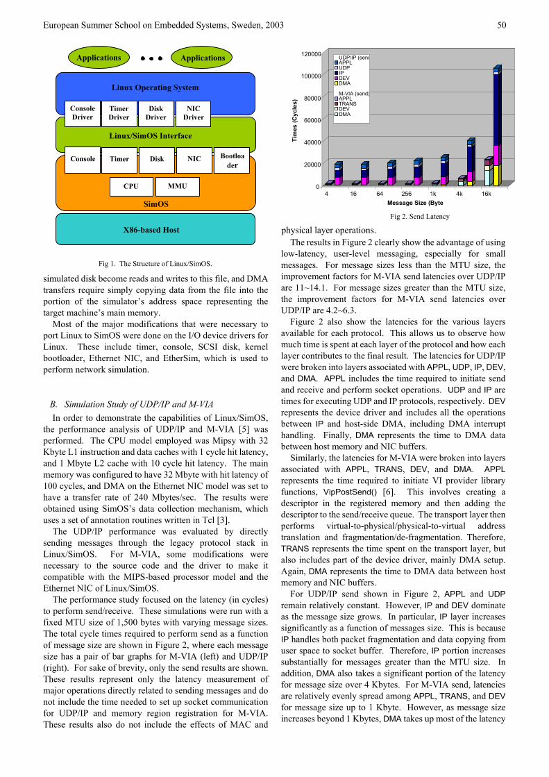
European Summer School on Embedded Systems, Sweden, 2003 50
simulated disk become reads and writes to this file, and DMA transfers require simply copying data from the file into the portion of the simulator’s address space representing the target machine’s main memory.
Most of the major modifications that were necessary to port Linux to SimOS were done on the I/O device drivers for Linux. These include timer, console, SCSI disk, kernel bootloader, Ethernet NIC, and EtherSim, which is used to perform network simulation.
B. Simulation Study of UDP/IP and M-VIA In order to demonstrate the capabilities of Linux/SimOS,
the performance analysis of UDP/IP and M-VIA [5] was performed. The CPU model employed was Mipsy with 32 Kbyte L1 instruction and data caches with 1 cycle hit latency, and 1 Mbyte L2 cache with 10 cycle hit latency. The main memory was configured to have 32 Mbyte with hit latency of 100 cycles, and DMA on the Ethernet NIC model was set to have a transfer rate of 240 Mbytes/sec. The results were obtained using SimOS’s data collection mechanism, which uses a set of annotation routines written in Tcl [3].
The UDP/IP performance was evaluated by directly sending messages through the legacy protocol stack in Linux/SimOS. For M-VIA, some modifications were necessary to the source code and the driver to make it compatible with the MIPS-based processor model and the Ethernet NIC of Linux/SimOS.
The performance study focused on the latency (in cycles) to perform send/receive. These simulations were run with a fixed MTU size of 1,500 bytes with varying message sizes. The total cycle times required to perform send as a function of message size are shown in Figure 2, where each message size has a pair of bar graphs for M-VIA (left) and UDP/IP (right). For sake of brevity, only the send results are shown. These results represent only the latency measurement of major operations directly related to sending messages and do not include the time needed to set up socket communication for UDP/IP and memory region registration for M-VIA. These results also do not include the effects of MAC and
physical layer operations.
0
20000
40000
60000
80000
100000
120000
Tim
es (C
ycle
s)
4 16 64 256 1k 4k 16kMessage Size (Byte
UDP/IP (sendAPPLUDPIPDEVDMA
M-VIA (send)APPLTRANSDEVDMA
Applications Applications
The results in Figure 2 clearly show the advantage of using low-latency, user-level messaging, especially for small messages. For message sizes less than the MTU size, the improvement factors for M-VIA send latencies over UDP/IP are 11~14.1. For message sizes greater than the MTU size, the improvement factors for M-VIA send latencies over UDP/IP are 4.2~6.3.
Figure 2 also show the latencies for the various layers available for each protocol. This allows us to observe how much time is spent at each layer of the protocol and how each layer contributes to the final result. The latencies for UDP/IP were broken into layers associated with APPL, UDP, IP, DEV, and DMA. APPL includes the time required to initiate send and receive and perform socket operations. UDP and IP are times for executing UDP and IP protocols, respectively. DEV represents the device driver and includes all the operations between IP and host-side DMA, including DMA interrupt handling. Finally, DMA represents the time to DMA data between host memory and NIC buffers.
Similarly, the latencies for M-VIA were broken into layers associated with APPL, TRANS, DEV, and DMA. APPL represents the time required to initiate VI provider library functions, VipPostSend() [6]. This involves creating a descriptor in the registered memory and then adding the descriptor to the send/receive queue. The transport layer then performs virtual-to-physical/physical-to-virtual address translation and fragmentation/de-fragmentation. Therefore, TRANS represents the time spent on the transport layer, but also includes part of the device driver, mainly DMA setup. Again, DMA represents the time to DMA data between host memory and NIC buffers.
For UDP/IP send shown in Figure 2, APPL and UDP remain relatively constant. However, IP and DEV dominate as the message size grows. In particular, IP layer increases significantly as a function of messages size. This is because IP handles both packet fragmentation and data copying from user space to socket buffer. Therefore, IP portion increases substantially for messages greater than the MTU size. In addition, DMA also takes a significant portion of the latency for message size over 4 Kbytes. For M-VIA send, latencies are relatively evenly spread among APPL, TRANS, and DEV for message size up to 1 Kbyte. However, as message size increases beyond 1 Kbytes, DMA takes up most of the latency
Fig 2. Send Latency
X86-based Host
SimOS
Linux Operating System
Console Driver
Timer Driver
DiskDriver
NIC Driver
Linux/SimOS Interface
Bootloader
NIC Console Timer Disk
MMU CPU
Fig 1. The Structure of Linux/SimOS.

European Summer School on Embedded Systems, Sweden, 2003 51Host processor DMA transfers
and increases rapidly. TRANS and DEV also increase significantly for message sizes larger than 1 Kbytes due to fragmentation and interrupt handling, respectively.
For DEV and DMA layers, both UDP/IP and M-VIA protocols show similar results. This is because M-VIA uses a same type of device driver to communicate with the Ethernet NIC model. The primary function of the DEV layer is to set up NIC’s DMA and receive interrupts from NIC. As can be seen, the latency of DEV remains relatively constant for message size up to 1 K bytes, but increases significantly when the messages are larger than the MTU size. DMA also varies linearly with the message size. This is consistent since DMA initiation and interrupt handling are already reflected in the DEV layer; therefore, DMA transfer time is dependent only on the message size.
C. Reducing Communication Latency Based on the aforementioned analysis of communication
protocols, it is obvious that the data transfer time between the host memory and network interface constitutes a significant portion of the overall communication latency. Therefore, this section explores a new data transfer mechanism to reduce this performance gap. The approach called Cache-Coherent Data Transfer (CC-DT) [13] is a special hardware structure that efficiently transfers data between the host and NI using the underlying cache coherence protocol. The CC-DT mechanism improves the performance by performing data transfer completely in hardware. Therefore, unlike DMA or CNI [10], there is no additional software overhead involved in data transfer and the memory bus bandwidth is efficiently efficient used since data transfers are done in cache block units. The proposed CC-DT together with an off-kernel VIA, called SonicVIA, was modeled and implemented as a NI module on Linux/SimOS. This allows us to capture all aspects of the communication performance, including the effects of the application, network protocol, and network interface.
Figure 3 illustrates the critical difference between a normal DMA transfer and CC-DT. As can be seen, there is a time interval between when the user process writes data to the user buffer (T2) and when data is DMA from the user buffer to NI
buffer (T5). Since this time accounts for a significant portion of the overall latency, the primary motivation of CC-DT is to overlap the execution of the user data writes and the DMA transfer of data to NI buffer to reduce the overall latency for message send/receive. CC-DT efficiently transfers data between the user buffer in the registered memory region and NI buffer allocated in NI local memory. This is accomplished by a special cache controller in NI that detects any accesses to the registered memory region, and maintains data coherence between the two associated buffers (see [13] for details).
Data(NI)
Descriptor (NI)
Doorbell Descriptor Data
Time
T1 T2 T3 T4 T5
(a) Data transfer using DMA.
Host processor writes
Doorbell Descriptor Data
Cache transfers (cache fill )
The total execution times required to perform a send+receive between two users as function of message size is shown in Figure 4. For each message size, there are three bar graphs representing the execution times of CC-DT (left), C-DMA (middle), and DMA (right). As can be see in the figure, the CC-DT mechanism results in much better performance compared to DMA and C-DMA [11]. The CC-DT-based NI attains 9% to 43 % reduction in the user-to-user messaging latency compared to the C-DMA-based NI. More importantly, the performance improvement becomes more significant as message size increases.
Descriptor (NI)
Data (NI)
Time
In order to gain a better understanding of the performance improvement, Figure 4 also shows the total execution times subdivided into three most significant sections in user-to-user communication: User Data, DMA, and Transport. The User Data section is the time required for the user program to write a message to the user buffer. The DMA section includes the time for DMA setup, DMA operations, and handling interrupts after DMA operations complete. The Transport section represents the time required to run the network protocol to service the user send/receive requests.
The breakdown view of the total execution time in Figure 4 clearly shows how significantly each section affects the overall latency and increases as data size grows. In particular, the amount of time spent on the DMA section depends on the underlying data transfer mechanism. The DMA sections for C-DMA are smaller than the ones for DMA. This is because C-DMA engines support cache-to-cache transfer so that the user data and descriptor can be moved directly from the cache memory on host processor. In contrast, DMA engines require two steps to move the user data from the cache memory: The user data in the cache memory has to be first flushed to the host memory and then moved to the NI buffer. Notice that there is no DMA section for CC-DT because the
T1 T2 TT5 T4 3
(b) Data transfer using CC-DT. Fig 3. DMA vs. CC-DT.
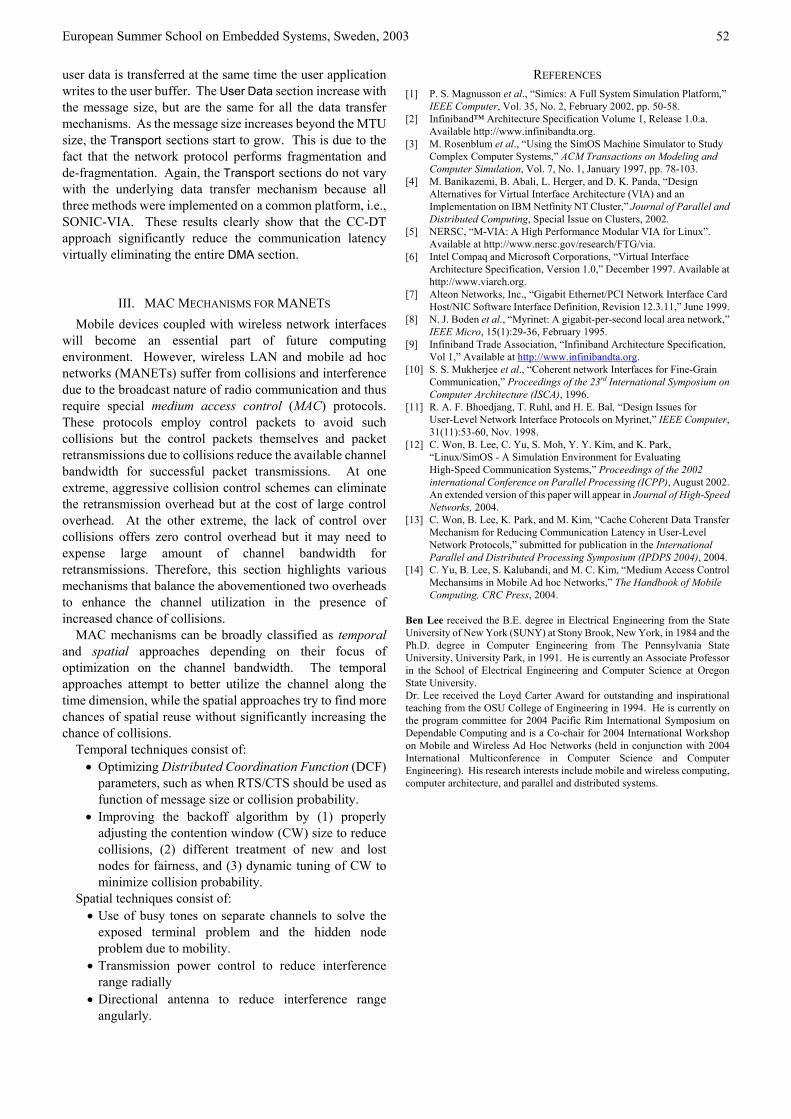
European Summer School on Embedded Systems, Sweden, 2003 52
user data is transferred at the same time the user application writes to the user buffer. The User Data section increase with the message size, but are the same for all the data transfer mechanisms. As the message size increases beyond the MTU size, the Transport sections start to grow. This is due to the fact that the network protocol performs fragmentation and de-fragmentation. Again, the Transport sections do not vary with the underlying data transfer mechanism because all three methods were implemented on a common platform, i.e., SONIC-VIA. These results clearly show that the CC-DT approach significantly reduce the communication latency virtually eliminating the entire DMA section.
III. MAC MECHANISMS FOR MANETS Mobile devices coupled with wireless network interfaces
will become an essential part of future computing environment. However, wireless LAN and mobile ad hoc networks (MANETs) suffer from collisions and interference due to the broadcast nature of radio communication and thus require special medium access control (MAC) protocols. These protocols employ control packets to avoid such collisions but the control packets themselves and packet retransmissions due to collisions reduce the available channel bandwidth for successful packet transmissions. At one extreme, aggressive collision control schemes can eliminate the retransmission overhead but at the cost of large control overhead. At the other extreme, the lack of control over collisions offers zero control overhead but it may need to expense large amount of channel bandwidth for retransmissions. Therefore, this section highlights various mechanisms that balance the abovementioned two overheads to enhance the channel utilization in the presence of increased chance of collisions.
MAC mechanisms can be broadly classified as temporal and spatial approaches depending on their focus of optimization on the channel bandwidth. The temporal approaches attempt to better utilize the channel along the time dimension, while the spatial approaches try to find more chances of spatial reuse without significantly increasing the chance of collisions.
Temporal techniques consist of: • Optimizing Distributed Coordination Function (DCF)
parameters, such as when RTS/CTS should be used as function of message size or collision probability.
• Improving the backoff algorithm by (1) properly adjusting the contention window (CW) size to reduce collisions, (2) different treatment of new and lost nodes for fairness, and (3) dynamic tuning of CW to minimize collision probability.
Spatial techniques consist of: • Use of busy tones on separate channels to solve the
exposed terminal problem and the hidden node problem due to mobility.
• Transmission power control to reduce interference range radially
• Directional antenna to reduce interference range angularly.
REFERENCES [1] P. S. Magnusson et al., “Simics: A Full System Simulation Platform,”
IEEE Computer, Vol. 35, No. 2, February 2002, pp. 50-58. [2] Infiniband™ Architecture Specification Volume 1, Release 1.0.a.
Available http://www.infinibandta.org. [3] M. Rosenblum et al., “Using the SimOS Machine Simulator to Study
Complex Computer Systems,” ACM Transactions on Modeling and Computer Simulation, Vol. 7, No. 1, January 1997, pp. 78-103.
[4] M. Banikazemi, B. Abali, L. Herger, and D. K. Panda, “Design Alternatives for Virtual Interface Architecture (VIA) and an Implementation on IBM Netfinity NT Cluster,” Journal of Parallel and Distributed Computing, Special Issue on Clusters, 2002.
[5] NERSC, “M-VIA: A High Performance Modular VIA for Linux”. Available at http://www.nersc.gov/research/FTG/via.
[6] Intel Compaq and Microsoft Corporations, “Virtual Interface Architecture Specification, Version 1.0,” December 1997. Available at http://www.viarch.org.
[7] Alteon Networks, Inc., “Gigabit Ethernet/PCI Network Interface Card Host/NIC Software Interface Definition, Revision 12.3.11,” June 1999.
[8] N. J. Boden et al., “Myrinet: A gigabit-per-second local area network,” IEEE Micro, 15(1):29-36, February 1995.
[9] Infiniband Trade Association, “Infiniband Architecture Specification, Vol 1,” Available at http://www.infinibandta.org.
[10] S. S. Mukherjee et al., “Coherent network Interfaces for Fine-Grain Communication,” Proceedings of the 23rd International Symposium on Computer Architecture (ISCA), 1996.
[11] R. A. F. Bhoedjang, T. Ruhl, and H. E. Bal, “Design Issues for User-Level Network Interface Protocols on Myrinet,” IEEE Computer, 31(11):53-60, Nov. 1998.
[12] C. Won, B. Lee, C. Yu, S. Moh, Y. Y. Kim, and K. Park, “Linux/SimOS - A Simulation Environment for Evaluating High-Speed Communication Systems,” Proceedings of the 2002 international Conference on Parallel Processing (ICPP), August 2002. An extended version of this paper will appear in Journal of High-Speed Networks, 2004.
[13] C. Won, B. Lee, K. Park, and M. Kim, “Cache Coherent Data Transfer Mechanism for Reducing Communication Latency in User-Level Network Protocols,” submitted for publication in the International Parallel and Distributed Processing Symposium (IPDPS 2004), 2004.
[14] C. Yu, B. Lee, S. Kalubandi, and M. C. Kim, “Medium Access Control Mechansims in Mobile Ad hoc Networks,” The Handbook of Mobile Computing, CRC Press, 2004.
Ben Lee received the B.E. degree in Electrical Engineering from the State University of New York (SUNY) at Stony Brook, New York, in 1984 and the Ph.D. degree in Computer Engineering from The Pennsylvania State University, University Park, in 1991. He is currently an Associate Professor in the School of Electrical Engineering and Computer Science at Oregon State University. Dr. Lee received the Loyd Carter Award for outstanding and inspirational teaching from the OSU College of Engineering in 1994. He is currently on the program committee for 2004 Pacific Rim International Symposium on Dependable Computing and is a Co-chair for 2004 International Workshop on Mobile and Wireless Ad Hoc Networks (held in conjunction with 2004 International Multiconference in Computer Science and Computer Engineering). His research interests include mobile and wireless computing, computer architecture, and parallel and distributed systems.

System-Level Optimization based on GeneticAlgorithms
Marcus T. SchmitzDept. of Computerand Information Science
Embedded Systems Lab (ESLAB)Linkoping University
SE-531 83 Linkoping, SwedenEmail: [email protected]
Abstract— Genetic algorithms have been the subject of numer-ous investigations in the last decades, and they have been provento solve different search and optimization problems successfully.By imitating and applying the principles of natural selection,they are able to evolve solutions to real-world problems. One ofthese real-world problems is the automated design of embeddedcomputing systems.
In this extended abstract, we will first briefly discuss thegeneral theory of genetic algorithms and then demonstrate theirapplicability in the context of system-level design. In partic-ular two hard optimization problems are addressed: activityscheduling and application mapping of heterogeneous distributedsystems. Particularly, we will focus on multi-mode systems thatcontain dynamically voltage-scalable processing elements. Theoptimizations are carried out towards the fulfillment of multipledesign objectives, such as timing behavior, area requirements,and power consumption.
I. I NTRODUCTION
The complexity of embedded systems has increased dra-matically over the last decades. While initial systems offeredrestricted functionality that could be realized through “simple”application-specific circuitry (e.g., pocket calculators, digitalwatches, etc.), nowadays portable computing systems have toprovide workstation-like performance at low energy consump-tion in order to carried out computational-expensive multi-media applications over long battery-life times (for example,portable DVD players, MP3 players, cellular phones, PDAs,and so on). Along with the increasing complexity comes atense market pressure that has resulted in shrinking product lifecycles and shortening time-to-market windows. Both trends,the increasing complexity to due feature richness and theshortening time-to-market times, have resulted in the need forsophisticated design automation tools. Automating the system-level design of embedded computing systems is a difficult taskthat requires solving several subproblems, such as componentallocation, multi-processor scheduling, and application map-ping. Since some of these problems belong to the class ofNP-hard problems, optimal solution often can not be obtainedfor realistic problem instances. Therefore, effective heuristictechniques are essential to yield good (not necessarily optimal)synthesis results in relatively short optimization times. Onegeneral heuristic optimization technique, which can be usedfor a wide range of different problems, is given by the classof genetic algorithms (GAs).
In this paper, we will briefly outline how genetic algo-rithms can be used for system-level synthesis, considering, inparticular, architectures that contain dynamic voltage-scalablecomponents.
II. B RIEF INTRODUCTION TOGENETIC ALGORITHMS
Before going into details of the genetic algorithm-basedsystem-level synthesis technique, we will first introduce somefundamental knowledge regarding genetic algorithms and theirfunctionality.
Genetic algorithms have been first introduced by Holland[5]. By imitating the principles of natural selection and evo-lution on a population of solution candidates, they are ableto optimize solutions to real-world problems. Each solutioncandidate (individual) of the problem to be solved is rep-resented as a string (chromosome). Each solution is furtherassociated with a fitness which represents the solution quality.Based on this fitness, the individual solutions are ranked.Within each iteration (generation), the algorithm performsa probabilistic selection upon the ranked individuals (thehigher the rank, the higher the chance of being selected) andgives them the opportunity to reproduce by means of mating(crossover) with other individuals of the population pool. Thisreproduction results in new individuals (offsprings) that inheritcertain properties and features from the parent individuals, thusincreasing the probability to have higher solution quality. Theproduced offsprings replace individuals of lower fitness, whichdie out. Nevertheless, new individuals are not only producedthrough crossover operations, but also by randomly changing(mutation) genes of chromosomes, occasionally. This providesan additional possibility to enter unexplored regions in thesearch space. The GA evolves until a certain stop criterion isfulfilled. For example, a maximum number of generations havebeen excepted or improved individuals have not been foodover a certain amount of generations, and so on. Fig. 1 showsthis functionality of genetic algorithms in graphical form. Forfurther readings, the interested reader is referred to excellenttextbooks on this subject [2], [6].
III. SYSTEM-LEVEL SYNTHESIS
Modern embedded systems are often implemented asheterogeneous, distributed architectures. The required
European Summer School on Embedded Systems, Sweden, 2003 53

τ0 τ5 τ627 3 45 37
3 5 52 6 3 4
7 3 5 2 4 37
32 6 5 5 3 4
7 3 5
32 6
5 5 3 4
2 4 37
3 4 4 29 93
2 2 32 9 7 92 2 32 9 7 9
pointCrossoverτ τ ττ1 2 3 4
3 72 2 2
String 1
String 2
String 3
String 4
String 5
String 6 9 934 5
77
4 2
Parent 1
Parent 2
Child 1
Child 2
Solution pool
Selection
Insertion
2 32 9 7 95
Qua
lity
(Fitn
ess)
Mutate genes
Mutation Crossover
High
Low
Fitness assign.
Fig. 1. Principles of genetic algorithm
functionality is implemented via software that runs onprogrammable components (e.g., general-purpose processorsand DSPs) and via hardware (e.g., ASICs and FPGAs).Two important problems that need to be solved during thesystem-level synthesis are mapping and scheduling:Application mapping: Functional fragments (tasks) of thesystem specification have to be uniquely assigned to theindividual components of the architecture. Furthermore,communications between tasks mapped to differentcomponents need to be assigned to communication links.Activity scheduling: An execution order and the exactstart times of tasks and communications have to obtained,considering task interdependencies.
Certainly, the optimization of these two problems has to beperformed towards multiple objectives which are possibilitycompeting. These objectives include energy dissipation, timingbehavior (fulfillment of deadlines), and area/memory require-ments. For instance, executing a certain function in softwareis often less energy-efficient and more time consuming thanimplementing the same task in hardware. The purpose ofthe genetic algorithm-based synthesis approach presented inSection V is to solve these problems efficiently.
IV. PRELIMINARIES
In this section, we outline the used specification models andformulate the problem at hand.
A. System Specification
The abstract specification model we consider here is basedon a combination of finite state machines and task graphs, usedto capture the interaction between different operational modesas well as the functionality of each individual mode. We referto this model as operational mode state machine (OMSM). Thefollowing section explains this model, using the smart phoneexample shown in Fig. 2. This smart phone combines threedifferent functionalities within one device: a GSM phone, adigital camera, and an MP3-player.
1) Top-level Finite State Machine: We consider that anapplication is given as a directed, cyclic graphΥ(Ω, Θ), whichrepresents a finite state machine. Within this top-level model,each nodeO ∈ Ω refers to an operational mode and eachedge T ∈ Θ specifies a transition between two modes. Ifthe system undergoes a change from modeOx to modeOy,with x = y, the transition timetmax
T associated with the
GSMcodec+ RLC
Ψ =0.741Ψ =0.012
Ψ =0.023
Ψ =0.024
Ψ =0.15Ψ =0.016
Ψ =0.017
Ψ =0.090
Radio Link Control
decode Photo
=0.025s
HD
deQ
IDCT
Tr.color
coeff.
256
256
256
256
RLC =0.015sθ
θ =0.025s
φ
SearchNetwork
RadioLink
Control
TakePhoto
Photodecode
Search+ Nework
Photo
+ RLC
+ RLCMP3 playMP3 play
+ NeworkSearch
Network found
Network lost
Network found
Network found
Network found
Network lost
ShowPhoto Photo
Show
Incoming CallUser request /
TerminateCall
audioPlay
audioPlay TerminateTerminate
audio audio
TerminateTerminatePhoto
Photo
Photo Phototaken taken
Take P
hotoTake Photo
decode
INIT
Fig. 2. Operational mode state machine and individual task graph specifica-tion
transition edgeT = (Ox, Oy) has to be met. At any given timethere is only one active mode, i.e., the modes are mutuallyexclusive. Fig. 2(a) exemplifies the operational mode statemachine for a smart phone example with eight different modes.An activation scenario could look like this: When switchedon, the phone initializes intoNetwork Search mode. Uponfinding a network, the phone changes intoRadio Link Control(RLC) mode. In this mode it maintains the connection tothe network by handling cell handovers, radio link failureresponses, and adaptive RF power control. An incoming phonecall necessitates to switch intoGSM codec + RLC mode. Thismode is responsible for speech encoding and decoding whilemaintaining network connectivity. Similarly, the remainingmodes have different functions and are activated upon modechange events. Such events originate upon user requests (e.g.MP3-player activation) or are initiated by the system itself(e.g. loss of network–switch back intonetwork search mode).
Based on the observation that many multi-mode systemsspend their operational timenot evenly in each of the modes,we assume that for each operational modeO its executionprobabilityΨO is given, i.e., we know what percentage of theoperational time the device spends in each mode. For instance,in accordance to Fig. 2(a), the smart phone stays 74% of thisoperational time inRadio Link Control (RLC) mode, 9% inGSMcodec + RLC mode, and 1% inNetwork Search mode. Theleft over 16% of the operation time are associated with theremaining modes.
2) Functional Specification of Individual Modes: The func-tional specification of each modeO ∈ Ω in the top-levelfinite state machine is expressed by a task graphGO
S (T , C);see Fig. 2(b). Here, each nodeτ ∈ T represents a task,an atomic unit of functionality that needs to be executedwithout preemption. We consider a coarse level of granularitywhere tasks refer to functions such as Huffman decoders, de-quantizers, FFTs, IDCTs, etc. Therefore, each task is furtherassociated with a task typeη ∈ ΓO. A distinctive featureof multi-mode systems is that task type setsΓO of differentmodesO ∈ Ω can intersect, i.e., tasks of identical type canshare the same hardware resource. Of course, resource sharingis also possible for multiple tasks of identical type which arefound in a single mode, however, due to task communalitiesamong different modes the chances to share resources areincreased. Edgesγ ∈ C in the task graph refer to precedence
European Summer School on Embedded Systems, Sweden, 2003 54
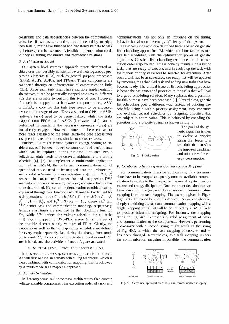
constraints and data dependencies between the computationaltasks, i.e., if two tasks,τi and τj , are connected by an edge,then taskτi must have finished and transfered its data to taskτj , beforeτj can be executed. A feasible implementation needsto obey all timing constraints and precedence relations.
B. Architectural Model
Our system-level synthesis approach targets distributed ar-chitectures that possibly consist of several heterogeneous pro-cessing elements (PEs), such as general purpose processors(GPPs), ASIPs, ASICs, and FPGAs. These components areconnected through an infrastructure of communication links(CLs). Since each task might have multiple implementationalternatives, it can be potentially mapped onto several differentPEs that are capable to perform this type of task. However,if a task is mapped to a hardware component, i.e., ASICor FPGA, a core for this task type needs to be allocated,involving the usage of area. Tasks assigned to GPPs or ASIPs(software tasks) need to be sequentialized whilst the tasksmapped onto FPGAs and ASICs (hardware tasks) can beperformed in parallel if the necessary resources (cores) arenot already engaged. However, contention between two ormore tasks assigned to the same hardware core necessitatesa sequential execution order, similar to software tasks.
Further, PEs might feature dynamic voltage scaling to en-able a tradeoff between power consumption and performancewhich can be exploited during run-time. For such PEs avoltage schedule needs to be derived, additionally to a timingschedule [4], [7]. To implement a multi-mode applicationcaptured as OMSM, the tasks and communications of alloperational modes need to be mapped onto the architecture,and a validschedule for these activitiesε ∈ (A = T ∪ C)needs to be constructed. Further, for tasks mapped to DVSenabled components an energy reducing voltage schedule hasto be determined. Hence, an implementation candidate can beexpressed through four functions which need to be derived foreach operational modeO ∈ Ω: MO
τ : T → π, MOγ : C → λ,
SOε : A → R
+0 , and V O
τ : TDV S → Vπ, where MOτ and
MOγ denote task and communication mapping, respectively.
Activity start times are specified by the scheduling functionSO
ε , while V Oτ defines the voltage schedule for all tasks
τ ∈ TDV S mapped to DVS-PEs, whereVπ is the set ofthe possible discrete supply voltages of PEπ. Clearly, themappings as well as the corresponding schedules are definedfor every mode separately, i.e., during the change from modeOx to modeOy, the execution of activities found in modeOx
are finished, and the activities of modeOy are activated.
V. SYSTEM-LEVEL SYNTHESIS BASED ONGAS
In this section, atwo-step synthesis approach is introduced.We will first outline an activity scheduling technique, which isthen combined with communication mapping. This is followedby a multi-mode task mapping approach.
A. Activity Scheduling
In heterogeneous multiprocessor architectures that containvoltage-scalable components, the execution order of tasks and
communications has not only an influence on the timingbehavior but also on the energy-efficiency of the system.
The scheduling technique described here is based on geneticlist scheduling approaches [3], which combine fast construc-tive list scheduling with the optimization power of geneticalgorithms. Classical list scheduling techniques build an exe-cution order step-by-step. This is done by maintaining a list oftasks that are ready to execute, and in each step the task withthe highest priority value will be selected for execution. Aftersuch a task has been scheduled, the ready list will be updatedby removing the scheduled task and adding new tasks that havebecome ready. The critical issue of list scheduling approachesis hence the assignment of priorities to the tasks that will leadto a good scheduling solution. Many sophisticated algorithmsfor this purpose have been proposed [1]. Nevertheless, geneticlist scheduling goes a different way. Instead of building oneschedule using a single priority assignment, they constructand evaluate several schedules by assigning priorities thatare subject to optimization. This is achieved by encoding thepriorities into a priority string, as shown in Fig. 3.
The goal of the ge-
τ4 τ5 τ6
7
Task τ τ τ τ0 1 2 3
τ0
PriorityString
7
τ
τ2
τ
τ1τ
τ
3
4 5 6θ θ θ654
4 98
1
4 8 9 1 3 2
23
Fig. 3. Priority string
netic algorithm is thento evolve a prioritystring that leads to aschedule that satisfiesthe imposed deadlinesand minimizes the en-ergy consumption.
B. Combined Scheduling and Communication Mapping
For communication intensive applications, data transmis-sions have to be mapped adequately onto the available commu-nication links, due to their impact on the overall system perfor-mance and energy dissipation. One important decision that wehave taken in this regard, was the separation of communicationmapping from the task mapping. The example given in Fig. 4highlights the reason behind this decision. As we can observe,simply combining the task and communication mapping with asingle mapping string that will be optimized by a GA is likelyto produce infeasible offspring. For instance, the mappingstring in Fig. 4(b) represents a valid assignment of tasksand communication to the components. However, performinga crossover with a second string might result in the stringof Fig. 4(c), in which the task mapping of tasksτ1 and τ2
has been changed. Nevertheless, this task mapping rendersthe communication mapping impossible: the communication
τ0 τ1 τ2 γ0−1γ1−2
γ0−1 γ1−2
τ0 τ1 τ2 γ0−1γ1−2
τ0 τ2 τ1γ1−2γ0−1
τ0 τ1 τ2
τ0
τ1
τ2 0 1 2 1 2
PE2PE1PE0
CL2CL1
Genetic0 2 1 1 2
PE2PE1PE0
CL1 CL2
CL3
CL0
CL3
CL0
operation
(a) Task graph (b) valid mapping string (c) invalid mapping string
Fig. 4. Combined optimization of task and communication mapping
European Summer School on Embedded Systems, Sweden, 2003 55
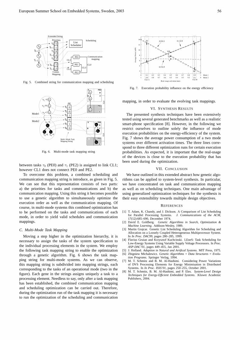
τ1
τ0
τ2
γ1−2
γ0−1
τ0γ0−1
τ1γ1−2
τ2
γ0−1γ1−2
SchedulerList
Priorities
Comm.Mapping
.
.
.
Extended String
Communicationmapping
PE0
PE1
PE2
CL0
CL1
CL2CL3
Scheduling
2
1
4
9
1
2
5
Fig. 5. Combined string for communication mapping and scheduling
PE0A
B
C
D
E
F
τ4
τ6
τ5
PE1
CL0
τ1
τ2
τ3
PE0A
B
C
D
E
F
PE1C
L0
η4=D
τ1
τ2
τ3
τ4
τ5
τ6
η1=A
η2=B
η3=C τ3
Multi−Mode TaskMapping String
η5=E
τ4
6τ5 τ
PE
Mode2
Mode1
0
1
0
0
1
0
η6=F
τ2
τ1
Fig. 6. Multi-mode task mapping string
between tasksτ0 (PE0) andτ1 (PE2) is assigned to link CL1;however CL1 does not connect PE0 and PE2.
To overcome this problem, a combined scheduling andcommunication mapping string is introduce, as given in Fig. 5.We can see that this representation consists of two parts:a) the priorities for tasks and communications and b) thecommunication mapping. Using this string it becomes possibleto use a genetic algorithm to simultaneously optimize theexecution order as well as the communication mapping. Ofcourse, in multi-mode systems this combined optimization hasto be performed on the tasks and communications of eachmode, in order to yield valid schedules and communicationmappings.
C. Multi-Mode Task Mapping
Moving a step higher in the optimization hierarchy, it isnecessary to assign the tasks of the system specification tothe individual processing elements in the system. We employthe following task mapping string to enable the optimizationthrough a genetic algorithm. Fig. 6 shows the task map-ping string for multi-mode systems. As we can observe,this mapping string is subdivided into mapping strings, eachcorresponding to the tasks of an operational mode (two in thefigure). Each gene in the strings assigns uniquely a task to aprocessing element. Needless to say, only after a task mappinghas been established, the combined communication mappingand scheduling optimization can be carried out. Therefore,during the optimization run of the task mapping it is necessaryto run the optimization of the scheduling and communication
Real−usage activation times
Ave
rage
Pow
er (
mW
)
User A User B
0.9:0.1 0.1:0.9
0.5:0.5
II
I
VII
VI
0 0.1 0.2 0.3 0.4 0.5 0.6 0.7 0.8 0.9 1
1 0.9 0.8 0.7 0.6 0.5 0.4 0.3 0.2 0.1 0
Mode 1
Mode 2
12
10
8
6
4
2 III
V
IV14
Fig. 7. Execution probability influence on the energy efficiency
mapping, in order to evaluate the evolving task mappings.
VI. SYNTHESIS RESULTS
The presented synthesis techniques have been extensivelytested using several generated benchmarks as well as a realisticsmart-phone specification [8]. However, in the following werestrict ourselves to outline solely the influence of modeexecution probabilities on the energy-efficiency of the system.Fig. 7 shows the average power consumption of a two modesystems over different activation times. The three lines corre-spond to three different optimization runs for certain executionprobabilities. As expected, it is important that the real-usageof the devices is close to the execution probability that hasbeen used during the optimization.
VII. C ONCLUSION
We have outlined in this extended abstract how genetic algo-rithms can be applied to system-level synthesis. In particular,we have concentrated on task and communication mappingas well as on scheduling techniques. One main advantage ofusing generalized optimization techniques for the synthesis istheir easy extensibility towards multiple design objectives.
REFERENCES
[1] T. Adam, K. Chandy, and J. Dickson. A Comparison of List Schedulingfor Parallel Processing Systems.J. Communications of the ACM,17(12):685–690, December 1974.
[2] David E. Goldberg. Genetic Algorithms in Search, Optimization &Machine Learning. Addison-Wesley, 1989.
[3] Martin Grajcar. Genetic List Scheduling Algorithm for Scheduling andAllocation on a Loosely Coupled Heterogeneous Multiprocessor System.In In Proc. DAC99, pages 280–285, 1999.
[4] Flavius Gruian and Krzysztof Kuchcinski. LEneS: Task Scheduling forLow-Energy Systems Using Variable Supply Voltage Processors. InProc.ASP-DAC’01, pages 449–455, Jan 2001.
[5] J. Holland. Adaption in Natural and Artifical Systems. MIT Press, 1975.[6] Zbigniew Michalewicz.Genetic Algorithms + Data Structures = Evolu-
tion Programs. Springer Verlag, 1994.[7] M. T. Schmitz and B. M. Al-Hashimi. Considering Power Variations
of DVS Processing Elements for Energy Minimisation in DistributedSystems. InIn Proc. ISSS’01, pages 250–255, October 2001.
[8] M. T. Schmitz, B. M. Al-Hashimi, and P. Eles.System-Level DesignTechniques for Energy-Efficient Embedded Systems. Kluwer AcademicPublishers, 2004.
European Summer School on Embedded Systems, Sweden, 2003 56

Predictability of Real-Time Software on Commodity Platforms
Jane W. S. Liu, Fellow, IEEE
I. BACKGROUND
This lecture focuses on means to make real-timeapplications predictable when they run on general-purposeoperating systems. The past two decades have ushered intremendous advances in real-time technology. Today, thereare well-founded architectural principles, design guidelinesand best implementation practices for most real-time applications. All modern operating systems provide sufficientreal-time support, including means for static configuration ofreal-time components on multiple processors, non-pagedmemory for time-critical code and data, prioritization of activities based on their required response times, end-to-endpriority tracking across layers and components, prioritizedaccess to resources, and some form of priority inversioncontrol. There are also methods and tools with which a developer can determine with acceptable accuracy worst-caseexecution times of time-critical components and validaterigorously the schedulability of the components and the system as a whole. These advances have enabled event-driventime-critical applications to be as provable responsive as time-driven applications. The lecture starts by reviewing theseresults; further details can be found in the incomplete list ofgeneral references [1-5].
The second part of this lecture discusses the gaps betweenmany assumptions of real-time workload and system modelsand real-life applications and platforms. The gaps are oftenwide and unbridgeable. An example is the commonassumptions underlying many studies on multiprocessorscheduling: Jobs (threads) can be dispatched dynamicallyfrom a common priority queue for all processors, and a newlyready higher priority job preempts the lowest priority job inthe system. For the sake of scalability and performance,modern operating systems use a queue per processor. Because preempting the lowest priority job in the system as a rule canlead to high cache misses and cascaded context swaps, thekernel makes no attempt to locate and preempt the lowest priority job when dispatching a higher priority job. It isdifficult to implement algorithms based on an invalid systemmodel. Moreover, the gain in schedulable utilization throughdynamic dispatching is likely to be offset by loss in effectiveutilization due to higher overhead.
Jane W. S. Liu is with the OS Core Technology Group, WindowsDivision, Microsoft Corporation, Redmond, WA 98052, USA(email: [email protected]).
II. OPEN SYSTEM AND RESOURCE RESERVATION
The third part of this lecture talks about state-of-art supportsfor real-time applications on open platforms. A commonassumption underlying existing real-time techniques andstandards is that the system is closed. This assumption is byand large valid until recently. In the past, embedded and real-time applications, ranging from avionics and flightmanagement, medical instrumentation, process control,intelligent manufacturing, and C3I, ran exclusively ondedicated, closed platforms. Resource demands and real-timerequirements of all applications in the system are known. Thisknowledge makes it possible to control their resourcecontentions coherently and to predict their timing behavioraccurately.
In recent years, rapid growth in diversity and pervasiveness of embedded and real-time applications has increased thepressure on reducing their costs and has shortened the time fortheir deployment and upgrade. A consequence is the growingtrend to build such applications from components and runthem on open platforms. The open-system approach has manyadvantages: Widely available tools and building blocks cansignificantly lower development and deployment cost andtime; hardware and kernel abstractions enable the use of awider variety of devices and configurations; and the burden ofkeeping pace with advances in hardware and softwaretechnologies is off-loaded to platform developers.
An open environment contains independently developedsystem and application components. The lack of informationon their resource demands and inability to control theirbehavior make it impossible to ensure predictability of time-critical components in open systems without some form of reservation.
Resource reservation was first proposed by C. Mercer as a way to ensure the quality of services of multimediaapplications [6]. Subsequently, the concept has been refinedand extended to support real-time guarantees (e.g., [7-9]) andresource sharing (e.g., [10].) Several experimental andcommercial prototypes (e.g., [7, 11, and 12]) havedemonstrated that resource reservation is feasible andeffective. By providing each time-critical component withtiming isolation and protecting it from ill effects of resourcecontention, resource reservation makes it possible to test,verify and tune the timing behavior of the component withoutregard to how other components in the system are scheduled.
European Summer School on Embedded Systems, Sweden, 2003 57

III. PROCESSOR TIME GUARANTEE
By far, processor reservation is the most mature comparedwith reservation mechanisms for other types of time-sharedresources. A processor reserve is a fractional bandwidth of aprocessor. When there is a reserve (P, B) with period P andbudget B (B < P) on a processor, the system commits todeliver B units of time of that processor to the reserve every period. Thus, the reserve is guaranteed the fraction B/P of theprocessor bandwidth. Since the budget of each period isdelivered by the end of the period, the period P is its latencyguarantee. Once admitted and created, threads (and processes)can be put in the reserve, meaning that they share theprocessor time allocated to the reserve.
There are many ways to support processor reserves. A common alternative is to put processor reserves in middleware and user levels. This is the approach taken byResource Kernels, RK/NT and Linux/RT [11] and by Auremaresource manager [12]. Portability is a major advantage of thisalternative. However, compared with kernel-level reserves,middleware- and user-level processor reserves generally havehigher overhead. More importantly, a middleware- or user-level reserve mechanism cannot efficiently support smalllatency (1-5 ms) guarantee and sub-millisecond budgetgranularity required by some applications.
For this reason, processor reserves are provided by thekernel in a future version of Microsoft Windows. Unlike theIllinois prototype [7], which provides completion timeguarantee, the reserve mechanism is designed to providebandwidth-latency guarantee to both sporadic and periodicexecutions of threads from real-time and general-purposeapplications. Conceptually, a reserve (P, B) can be thought ofas a constant utilization server. At each replenishment time,the reserve is given its budget B, and its deadline is set at current time plus P so that the instantaneous utilization of thereserve is equal to its bandwidth. A reserve is eligible forscheduling when it has budget and at least one thread in it isready to run. When a reserve has no ready-to-run thread, its budget is reclaimed and made available to threads runningwithout reserves. Eligible reserves are scheduled on theearliest-deadline-first (EDF) basis. Whenever a reserve isscheduled, the highest priority thread among threads in thereserve runs, regardless its priority relative to priorities ofthreads not in the reserve. Thus, the reserve protects threads init from conflicting prioritization of threads outside the reserve.The system monitors the processor time consumed by threadsin the reserve and stops scheduling the reserve (and hencethreads in it) when the threads exhaust the reserve budget. Thereserve becomes eligible for scheduling again when thesystem replenishes its budget at its deadline.
One may question why not replenish and scheduleprocessor reserves according to the total bandwidth server(TBS) algorithm instead of constant utilization server. It is well known that TBS and its many variants yield betteraverage response time and naturally allow exhausted reservesto share background processor time left unused by reserves.TBS would be a better choice if every thread in the system
runs in some reserve. On an open platform, most applications,drivers and system components do not use reserves. Theirthreads run without reserves. If reserves were scheduledaccording to the TBS algorithm, run-away threads in somereserve would starve these threads. Soft reserves (i.e., reservesthat are allowed to compete for background time after theyexhausted their budgets) need to be scheduled in thebackground of threads without reserves.
IV. DISK BANDWIDTH RESERVATION
Despite of numerous studies on real-time disk scheduling,algorithms suitable for disk bandwidth reservation in an openplatform are yet to be found in literature. Most real-time diskscheduling algorithms are variants of EDF or least slack time(LST) algorithms. Their primary goal is to maximizeschedulable utilization of real-time requests; keepingthroughput high is secondary. An example is the EDF-scanalgorithm. According to this algorithm, in each seek, the R/Whead moves in the direction of the request with the earliest deadline, but stops to pick up requests along the way to thatrequest for as long as the request has slack or the current timeis within a window of some threshold length. A potentialadvantage of the algorithm is a higher schedulable real-timebandwidth. However, it is not clear whether this advantage isin fact realizable when one takes into account the extra amount of seek time that may incur, and the extra seek time iswasted. In general, priority-based algorithms do not work wellwhen the server (in this case the R/W head) must walk from request to request. Starvation is also a problem and must bedealt with. Algorithms that use slack information have theadditional burden of slack computation. The computation can be complicated especially since the disk scheduler in an openplatform must work for all types of disks and volumeconfigurations (e.g., striped and mirrored).
Weighted-round-robin (WRR)-scan offers a morepractical solution. WRR-scan algorithm is a combination ofscan, WRR and time-token algorithms. It was motivated bythe following observations:
1. Similar to processor reserve, each disk reservation (P,N) is specified by period P and number N of datablocks per period: A user of the reservation can reador write N blocks of data every period of length P bythe end of the period. A stream of requests with a reservation behaves like a periodic task.
2. The problem of scheduling periodic requests in midstof interactive and paging requests resembles theproblem of scheduling periodic messagetransmissions in midst of aperiodic messages in aFDDI network. A timed-scan algorithm similar to theFDDI time-token protocol may work better thanpriority-based algorithms.
3. Unlike stations on a network, however, the diskscheduler has global knowledge of all outstandingrequests during each scan. This knowledge allowsthe use of a centralized scheme similar to the WRR
European Summer School on Embedded Systems, Sweden, 2003 58

scheme, which is used for scheduling periodic andaperiodic messages in packet-switched networks.
WRR-scan works like a standard scan algorithm: The R/W head starts from one end of the disk, seeks across the disktowards the other end, serves selected requests along the wayuntil it reaches the furthermost selected request, and then returns to the starting end and does the next scan. Thealgorithm differs from the standard scan only in its choices ofrequests to service and how much of each request to service during each scan. WRR-scan resembles the WRR scheme in the sense that it is rate-based. It also divides time into roundsand allocates to each periodic request stream a number of slots per round, where a slot is the time required to access a block of data. Like the timed-token protocol, WRR-scanalgorithm also must set aside “walking time”, the time takenby the R/W head to move from request to request and acrossthe disk.
The WRR-scan algorithm assumes that a new reservationis admitted only if it passes an acceptance test. The test is similar to the kind used for WRR algorithm: A newreservation (P, N) can be admitted only if within the P/Rrounds in each of its period, where R the maximum roundlength, there are enough unreserved slots to meet its demand.
To explain the algorithm with the aid of an example,suppose that the parameters of a disk are as follows:
1. The minimum amount of data to be transferred is ablock of 64kb. The transfer time of the block plusnominal seek and rotational latencies is 10 ms.
2. The chosen round length R is 200 ms. In otherwords, each round has at most 20 slots.
3. The degenerate round-trip seek time (walking time)of the disk is 50 ms. Hence 5 slots per round may be wasted in the worst case when requests serviced in the round are scattered across the disk. This timecan be used opportunistically for backgroundrequests if during any scan, the actual seek timeamong all outstanding requests is smaller than 50ms.
4. Three slots in each round are set aside to ensureacceptable response time for interactive requests.Therefore, only 12 slots out of each 200 ms round are available for requests with reservations.
5. The disk is divided into zones based on locations ofrequests with reservations.
Suppose that there is a reservation (300, 3) when a newreservation (500, 10) is subjected to acceptance test. (500, 10)is acceptable because within each period of length 500, thereare 2 rounds. The demand of (500, 10) can be met because thenumber of unreserved slots per round is larger than 5. After(500, 10) is admitted, 8 out of 12 slots of every round arereserved1. In the worst case, (200, 3) and (500, 10) are at the
first zone and last zone of the disk, respectively. So, five slotsare used just to shuttle the arm between them. The number ofslots available for interactive and background requests is atleast 7 per round. (Note that one out of 5 rounds, (500, 10) hasno pending transfer, and there are 12 slots available forinteractive and background requests in that round.) These slots can be distributed among pending interactive andbackground requests according to any strategy.
1 Note that the scheduler over commits slots for both reservations. A seemingly better alternative is to keep track the actual number of slots required by each reservation in each round. For this purpose,the scheduler would need to maintain a table of reserved slots in individual rounds. The length of the table is the least common
multiples of all possible periods. The additional memory required tohold the table is usually not a serious problem. More seriously, starts of rounds would have to be aligned with the starts of their periods if the scheduler were to take advantage of the additional slots in some rounds. This requirement would make scheduling and controlconsiderably more complex and less robust.
The example illustrates that WRR-scan gives the schedulergood control over tradeoff between average response time and throughput of interactive and paging requests and totalbandwidth made available to reservations. The amount ofslack that is available for interactive and paging requests in each round can be easily determined from the slots, locationsand pending flags of the requests with reservations.
VI. FUTURE WORK
A great deal of work remains to be done so that the predictability of real-time applications on open platforms canbe assured. The last part of the lecture discusses examples of missing sciences and technology.
An obvious missing piece is platform support for networkbandwidth and latency guarantees. Literatures offer numerousreal-time communication algorithms and protocols that can beused to support network bandwidth reservation and qualify-of-service management. Many prototype protocol stacksprovide bandwidth and latency guarantees. The fragmentedresults are yet to be integrated into widely used platforms andnetworks and their effectiveness for common applications andscenarios thoroughly evaluated.
A frequently asked question from application developers is“how do we know the amount of processor bandwidth toreserve”. This question points to another example of missingtechniques. Existing worst-case execution time analysis methods and tools cannot provide answer to this question. Acomponent (e.g., an audio engine, a Kalman filter) in an opensystem may run on hundreds of different computers, differentversions of operating systems, and depending on the runtimeenvironment, makes use of different libraries, etc. At differenttimes, hyper-threading may be on or off, and a variety ofworkload may run on other logical processors. Clearly, a static profile of the resource demands of a component is notuseful. Dynamic runtime profiling and calibration can providedata on resource demands. The problem is not that there are no tools for this purpose. Rather, it is the lack of soundprinciples and experiment methods based on which tools can be built.
European Summer School on Embedded Systems, Sweden, 2003 59

REFERENCES
[1] Proceedings of Euromicros, IEEE RTSS, and RTAS, 1985-2003.
[2] M.H. Klein, et al, A Practitioner’s Handbook for RMA,Kluwer Academic Publishers, 1993.
[3] J. W. S. Liu, Real-Time Systems, Prentice Hall, 2000 [4] G.C. Buttazzo, Hard Real-Time Computing Systems,
Kluwer Academic Publishers. [5] Q.Li and C. Yao, Real-Time Concepts for Embedded
Systems, CmpBooks.[6] C.W. Mercer, S. Savage, and H. Tokuda, “Processor
capacity reserve: operating system support formultimedia applications,” Proceedings of the IEEEConference on Multimedia Computing and Systems, May1994.
[7] Z. Deng, J. W. S. Liu, A. Frei, M. Seri and L. Zhang,“An open environment for real-time applications,” Real-Time Systems Journal, Vol. 16, No. 2/3, pp.155-186, May1999.
[8] T.W. Kuo, et al. “An open real-time environment forparallel and distributed systems,” Proceedings of ICDCS,2000.
[9] I. Shin and I. Lee, “Periodic resource model for compositional real-time guarantees,” Proceedings ofIEEE Real-Time Systems Symposium, 2003.
[10] A. Mok, X. Feng, and D. Chen, “Resource partition for real-time systems,” Proceedings of Real-TimeTechnology and Application Symposium, 2001.
[11] R. Rajkumar, J. Kanaka, A. Molano and S. Oikawa,“Resource kernel: a resource-centric approach to real-time systems,” Proceedings of the SPIE/ACM Conferenceon Multimedia Computing and Networking, January 1998.
[12] http://www.aurema.com.
European Summer School on Embedded Systems, Sweden, 2003 60

European Summer School on Embedded Systems, Sweden, 2003 61
Elements of Real Time Systems
Lui Sha
Lecture 1: Elements of Research The entrance to graduate school marks a critical phase of transition for most graduate students from absorbing knowledge to creating knowledge. This lecture provides useful advices on how to position R&D strategically; how to identify and formulate high impact problems; and how to communicate ideas and results effectively. Lecture 2: Generalized Rate Monotonic Scheduling GRMS was designed to support the resource management of real time control systems, which consists of mostly periodic tasks with a small percentage of aperiodic events. GRMS has now been supported by most Real Time Operating Systems and open standards in real time computing. This lecture provides a tutorial on this subject for students who are new to real time computing field. This lecture begins with a review of characteristics of real time systems that set them apart from general purpose computing systems. It reviews the basic real time scheduling topics of schedulability tests for periodic tasks, synchronization of real time tasks, and the handling of aperiodic events. References Sha, L. and Goodenough, L.,“Real-Time Scheduling Theory and Ada”, IEEE Computers, Vol. 23, No.4, pp. 53-62, April 1990. Klein, M., Ralya, T., Pollack, B., and Obenza, R., “A Practitioner's Handbook for Real-Time Analysis: Guide to Rate Monotonic Analysis for Real-Time Systems”, Kluwer, 1994. Lecture 3: Queueing Theory Based Network Server Performance Control Controlling the performance of a network server is a challenging problem in soft real time applications. This lecture presents a queuing model based feedback control approach to keep the timing performance of a network server close to the specification. The queueing predictor based feed forward control keeps the system in the neighborhood of the performance set point, independent of workload changes. This allows us to develop a linear controller to fine tune the performance by suppressing not only the approximation errors in the queueing model but also the transients that cannot be reduced by queueing model based tuning. Together, queueing theory and feedback control theory a synergistic approach to control the performance of networked information servers. References Sha, L., Li, X., Lu, Y., and Abdelzaher, T. “Queueing model based network server performance control”, the proceedings of IEEE Real-Time Systems Symposium, 2002 Lu, Y., Abdelzaher, T., Lu, C., Sha, L., and Xu, L., “Feedback Control with Queueing-Theoretic Prediction for Relative Delay Guarantees in Web Servers”, The 9th IEEE Real-Time and Embedded Technology and Applications Symposium, 2003.

European Summer School on Embedded Systems, Sweden, 2003 62
Lecture 4: Dependable Upgrade of Control Software How to improve the reliability and availability of complex software systems is a serious challenge as software assumes an increasingly larger role in the critical functions of our society. It is a widely held belief that using diversity in software systems will improve system reliability. However, is it true? This lecture investigates the relationship between software complexity, reliability, degree of diversity and available resource for software development. Based on the result of this analysis, we present a forward recovery approach based on the idea of “using simplicity to control complexity”. We show that this is an effective approach that can be applied systematically to software for automatic control systems. References Sha, L., “Using Simplicity to Control Complexity”, IEEE Software, July-August, 2001. Sha, L., “Upgrading real-time control software in the field”. Proceedings of the IEEE 91(7): 1131-1140 (2003)
European Summer School on Embedded Systems, Sweden, 2003 63
The Timing Behavior of Embedded Systems: Specification, Prediction, and Checking
Alan Shaw
Abstract—The survey is based primarily on my 2001
textbook, emphasizing methods to describe, analyze, measure, and predict the timing properties of embedded software. Topics include extended state machine and logic techniques for specification; schema and optimization approaches to prediction; and programming language and operating system facilities for checking and controlling timing behaviors.
Index Terms—Execution time prediction, real-time systems, real-time software, timing analysis, timing specifications
I. INTRODUCTION
AN essential determinant of the correctness of any embedded system is its timing behavior. This behavior
is measured not only by meeting performance or speed requirements, but often also by satisfying more complex, usually deterministic, constraints or assertions involving time.
We survey many of the models and techniques that have been used to deal with timing problems, starting with specification methods and working through to software support [1]. Most of the content appears in my textbook [2].
The first part gives a brief overview of embedded and real-time systems and a discussion of computer time and clocks [3]. In the following section, we outline several of the principal specification methods for describing requirements and designs, with emphasis on state machines, regular expressions, and real-time logic [4]. The next topic is how to predict the execution times of programs, using both timing schema and optimization approaches [5]. The final part is concerned with facilities in programming languages and operating systems that monitor and control time [6].
II. EMBEDDED SYSTEMS AND COMPUTER TIME Software for embedded and real-time systems differs from
conventional software in a number of significant ways, such as the importance of clocks and timing constraints, physical concurrency, reliability and fault tolerance, testing and certification, and stand-alone operation. The main scheme for modeling and implementing programs is the process model developed for operating systems. Two kinds of processes are defined to handle the application area: periodic processes and sporadic processes, the latter corresponding to interrupt- or
event-driven processes.
Manuscript received October 9, 2001. (Write the date on which you
submitted your paper for review.) Alan Shaw is with the Department of Computer Science and Engineering,
University of Washington, Seattle, WA 98195 USA (phone:206-543-9298; fax: 206-543-2969; e-mail: [email protected]).
Computer time and clocks are employed for a wide variety of purposes. Examples are time-stamping the occurrence of events to indicate causality (e.g., for message sends and receives), measuring the time between events (e.g., for deadlines), unique naming of objects, computing keys in cryptography, synchronizing activities, and precisely measuring distance and position (e.g., GPS). Computer time should have certain properties relative to ideal or standard time. These include correctness, bounded drift, monotonicity, and chronoscopicity (bounded 2nd derivative of the clock function).
Clock servers provide computer users a number of basic services related to time. Typical offerings are absolute (calendar) clock times, stopwatch or relative time, clock reset and clock set. To maintain desirable clock properties, clocks need to be synchronized with standard or other clocks. This may occur through a centralized standard, such as GPS, or via a distributed method whereby a number of clocks achieve internal synchronization by passing clock timestamps to one another.
III. SPECIFICATION METHODS Formalisms for describing the behavior of systems can be
classified as either imperative or declarative. In the first case, the methods are operational or executable, and directly generate behaviors. These include state machine and programming language notations. Declarative techniques, on the other hand, specify properties that behaviors must satisfy. Examples are axiomatic methods and logics.
The most interesting and difficult problems are concerned with concurrency and time. As typical solutions, we present useful extensions of state machines, regular expressions, and predicate logic.
Communicating real-time state machines (CRSMs) are an extension of state machines for a distributed real-time environment. Machines communicate (perform I/O with each other) over unidirectional channels through one-to-one message passing following Hoare’s CSP model. Each state transition, denoted by a guarded command, has associated time bounds that define the best and worst case execution times for the transition. For I/O commands, the time bounds represent the window during which I/O can occur. Corresponding to each CRSM is a clock machine, a simple CRSM that delivers real-time to its host on request and allows timeouts to be easily described.
CRSMs are universal machines, and admit to simulation and verification software. Transitions occur on an
European Summer School on Embedded Systems, Sweden, 2003 64
earliest-time first basis, with ties handled non-deterministically. Example systems that have been specified and simulated (or implemented) include: alarm clocks with ringing times and reset; mouse clickers with single click, double click, and object selection features; railway crossing control; traffic light control with emergency operations; and a commercial defibrillator.
A more declarative technique is the flow expression scheme, an extension of regular expressions with an interleaved model of concurrency. A shuffle operator and its closure are added to express the interleaving of symbols; restrictions on interleaving are described employing operators that are similar to binary semaphores. The result is a universal notation. The method has been used to specify ordering and causality properties, for example a “send” event must precede a “receive”. Time is included by including discrete clock tick events in descriptions.
The addition of an event-occurrence function to predicate logic has produced a powerful notation called real-time logic (RTL). This partial function maps instances of event classes into time. RTL has been used to describe a wide variety of safety properties of systems, such as deadlines or “two planes must maintain a given separation distance from each other”. It has also been implemented in run-time checkers where RTL expressions are evaluated at critical points to assure that constraints are met.
IV. PREDICTING EXECUTION TIMES Determining the best and worst case execution times of a
program before running it is not only a basic requirement for real-time and embedded systems but also a fundamental problem in computer science. While theoretically unsolvable in the general case, the problem can still be handled for many practical situations.
The difficulty is to achieve bounds that are both tight and safe, where a bound is tight if there exists an actual execution that is close to it and a bound is safe if there do not exist executions outside of it. It is also desirable to produce bounds that take into account or are independent of a variety of possible hardware or architectural interferences and complexities, such as interrupts and caching; and bounds that work under a variety of operating systems and compilers, and in the presence of competing programs. After a brief discussion of the two most practical, widely-used, but ultimately flawed approaches, measurement and simulation, we describe two promising methods: program analysis through timing schema and prediction through optimization techniques.
Correctly measuring the execution time of a particular program with its data in a given environment is not as easy as it appears, especially in embedded systems where computer components are closely coupled with other systems and I/O. It is also difficult, and often impractical, to find, run, and measure the best or worst case executions. Prediction by measurement also assumes that failure costs, for example, missing a deadline, are not catastrophic, and thus does not work well with safety-critical systems. Simulation avoids some, but not all, of these problems. In addition, one has to be careful to ensure that the results are practical despite the
inevitable abstractions that are made. Nevertheless, a combination of these two approaches, particularly for components or small systems, has proven successful.
The Timing schema method is based on program analysis at the source language level. It is assumed that best and worst case execution bounds are available for each basic or atomic component of the programming language, taking the compiler and machine architecture into account; the granularity or definition of an atomic component could be as large as a basic block or as small as a lexical item in the language. The timing costs of control constructs, for example, conditional testing and branching, are included. These times can be found, for example, by measurement.
Safe, but not necessarily tight, bounds on execution times are first obtained through a static analysis of the program structure. For example, a safe estimate of the worst case time is obtained by computing the longest path through the program. Much of this can be accomplished automatically. However, user input and verification is required for bounding the number of executions of loops.
Tighter estimates result when larger granularity atomic components are used and when a more dynamic analysis is superimposed. In the latter case, extended regular expressions have been employed successfully to describe contextual restrictions on program paths. It is also possible to accurately incorporate many hardware interferences; for example, executions in the presence of interrupts can be analyzed provided that bounds on interrupt separation times and handling times are available. The ideas have been validated with software tools through a number of experiments that compare measured results with predictions for a representative sample of relatively small programs.
Another attractive approach models timing prediction as an optimization problem. Worst (or best) case execution time is expressed as the maximum (or minimum) of a function that is the sum of the product of the execution time of each block of the program and the number of times it is executed; the number of times each block is executed is unknown. The function is subject to a number of structural constraints which essentially conserve program flow, and contextual constraints, such as loop bounds and path restrictions, that have to be verified independently. These constraints can be written as linear inequalities involving the unknown variables.
The result is a (potentially large) number of integer linear programming problems, each of which can be solved with a standard solver. The desired bound is computed by taking the maximum (or minimum) of all the solutions. This method has also been validated with many experiments.
A difficult underlying issue for both methods is how to accurately include many of the speed-enhancing features of the underlying hardware architectures. Examples include data and instruction caches, pipelining, and translation lookaside buffers. Much work has been done exploring this problem, for example, also using optimization techniques, but general solutions remain elusive. It could very well be that in order to obtain deterministic predictability, one must sacrifice gains in average speed.
European Summer School on Embedded Systems, Sweden, 2003 65
V. SOFWARE SUPPORT Many modern programming languages and operating
systems provide basic and higher level features that allow the user to control and measure the timing behavior of software for embedded systems. These include clock servers as outlined in Section II, alarm clocks that generate timeout events at some future time, instructions to delay a task or thread for some specified time, and blocking synchronization and resource acquisition operations that provide timeouts. An important feature of these facilities is that they include bounds on the timing accuracy and overhead; for example, a delay operation might include a guarantee that the delayed task will appear on a ready list within a given number of time units after expiration. Some research systems support higher-level specifications; a typical example is one that permits the direct declaration of a periodic process, including start time, period, and deadline.
Two well-known languages with good timing constructs are Ada with its real-time annex and real-time Java. In both cases, the timing facilities are high resolution, high accuracy, and monotonic versions of the analogous objects of the hosts (standard Ada and Java). In addition, real-time Java offers a novel timing object called rational time that deals in frequencies. Both languages also permit better management of concurrency, for example, including priority inheritance protocols which allow more scheduling control and thus timing predictability.
Many language features are directly implemented as operating systems interfaces or run-time utilities. Real-time versions of UNIX and the associated real-time extensions to the IEEE POSIX standard implement many of the mentioned clock facilities and define direct interfaces to programming languages.
REFERENCES [1] A. C. Shaw, “The timing behavior of embedded systems: specification,
prediction, and checking,” ESSES Lectures, cover slide. [2] ———, Real-Time Systems and Software, New York: John Wiley &
Sons, 2001. [3] ———, “Introduction,” ESSES Lectures, slide L1. [4] ———, “Specifications with time,” ESSES Lectures, slides L2.1 and
L2.2. [5] ——, “Predicting program execution times,” ESSES Lectures, slide
L3. [6] ———, “Software support for time,” ESSES Lectures, slide L4. Alan Shaw received the B.A.Sc. degree in engineering physics from the University of Toronto, Canada, in 1959, and the M.S. degree in mathematics and Ph.D. degree in computer science in 1962 and 1968, respectively, from Stanford University, USA. He has worked as a System Engineer with IBM and a Research Associate at the Stanford Linear Accelerator Center. He was a Visiting Professor at ETH, Zurich, the University of Paris, UC Santa Cruz, and Telecom, Paris, and a member of the faculty of the Department of Computer Science at Cornell University. He joined the faculty of the Department of Computer Science and Engineering at the University of Washington, Seattle, USA, in 1971, and is currently Professor Emeritus. He is the author of many research papers and several textbooks. Most recently, he published a text on real-time software and is coauthor of the textbook Operating Systems Principles (New Jersey: Prentice Hall, 2003). His current research interests are software specifications and real-time systems.
Prof. Shaw is a Fellow of the ACM and former Fulbright Research Scholar. His editorial board service has included IEEE Transactions on Software Engineering and Real-Time Systems Journal.

Stochastic Analysis of Real-Time SystemsKanghee Kim, Jos´e Luis Dıaz, Lucia Lo Bello, Jos´e Marıa Lopez,
Chang-Gun Lee, Daniel F. Garc´ıa, Sang Lyul Min, and Orazio Mirabella
Abstract— This paper describes an exact stochastic analysis forgeneral priority-driven periodic real-time systems. The proposedanalysis accurately computes the response time distribution ofeach task in the system, thus making it possible to determine thedeadline miss probability of individual tasks, even for systemswith a maximum utilization factor greater than 1. The analysis isuniformly applied to general priority-driven systems, includingfixed-priority systems (such as Rate Monotonic) and dynamic-priority systems (such as Earliest Deadline First), and canhandle tasks with arbitrary relative deadlines and executiontime distributions. In the paper, we demonstrate the accuracyof the analysis in comparison with other methods proposed inthe literature.
Index Terms— Real-time systems, Stochastic analysis, Priority-driven scheduling, Periodic tasks
I. I NTRODUCTION
Most recent research on hard real-time systems has usedthe periodic task model [1] in analyzing the schedulability ofa given task set where tasks are released periodically. Basedon this periodic task model, various schedulability analysismethods for priority-driven systems have been developed toprovide a deterministic guarantee that all the instances, calledjobs, of every task in the system meet their deadlines, assum-ing that every job in a task requires its worst case executiontime [1], [2], [3].
Although this deterministic timing guarantee is needed inhard real-time systems, it is too stringent for soft real-timeapplications that only require a probabilistic guarantee that thedeadline miss ratio of a task is below a given threshold. Forsoft real-time applications, we need to relax the assumptionthat every instance of a task requires the worst case executiontime in order to improve the system utilization.
Progress has recently been made in the analysis of real-timesystems under the stochastic assumption that jobs from a taskrequire variable execution times. Research in this area can becategorized into two groups depending on the approach used tofacilitate the analysis. The methods in the first group introducea pessimistic or restrictive assumption to simplify the analysis.
K. Kim ([email protected]) and S. L. Min ([email protected]), School of Computer Science and Engineering, Seoul National Uni-versity (Shillim-dong San 56-1, Kwanak-Gu, Seoul, 151-742 Korea). Thiswork was supported in part by the Ministry of Science and Technology underthe National Research Laboratory program and by the Ministry of Educationunder the BK21 program.
J. L. Dıaz, J. M. Lopez and D. F. Garc´ıa (jdiaz,chechu,[email protected]), Departamento de Inform´atica, Universidad de Oviedo(33204,Gijon, Spain)
L. Lo Bello and O. Mirabella (llobello,[email protected]), Dipar-timento di Ingegneria Informatica e delle Telecomunicazioni, Facolta diIngegneria, Universit`a di Catania(Viale A. Doria 6, 95125 Catania, Italy)
C.-G. Lee ([email protected]),Department of Electrical Engi-neering, Ohio State University(2015 Neil Avenue, Columbus, OH 43210,U.S.A.)
For example, the Stochastic Time Demand Analysis [4] triesto compute an upper on the deadline miss probability ofeach task assuming the worst-case combination of task releasetimes, called acritical instant. As another example, Real-Time Queueing Theory [5], [6] has a restrive assumption thatthe system to be analyzed should have an average systemutilization close to 1, calledheavy traffic conditions. On theother hand, the analysis methods in the second group [7], [8]assume areservation-based scheduling modelthat providesisolation between tasks, and thus decompose the stochasticanalysis of an entire system into those ofn independent virtualsystems (n: the number of tasks).
In this paper, we describe an exact stochastic analysis thatdoes not introduce any worst-case or restrictive assumptionsinto the analysis. The proposed analysis assumes neither acritical instant nor heavy-traffic conditions, thus can givean accurate deadline miss probability for each task in asystem with an arbitrary system utilization value. Moreover,the analysis assumes general priority-driven scheduling, thuscan uniformly address both fixed-priority systems such as RateMonotonic [1] and Deadline Monotonic [9] and dynamic-priority systems such as Earliest Deadline First [1]. It shouldbe noted that our analysis builds upon the Stochastic TimeDemand Analysis (STDA) in that we largely borrow the basictechniques developed in the STDA.
The rest of the paper is organized as follows. In Section II,we describe the system model, and in Section III, explain theproposed analysis. In Section IV, we give experimental resultsobtained by our analysis in comparison with STDA. Finally,in Section V, we conclude the paper with directions for futureresearch.
II. SYSTEM MODEL
We assume a set ofn independent periodic tasksτ1 τn, each taskτi (1 i n) being modeled by thetuple Ti φi Ci Di, whereTi is the period of the task,φi itsinitial phase,Ci its execution time, andDi its relative deadline.The execution timeCi is a discrete random variable with agiven probability mass function of a finite range, denotedby fCi t PCi t. The execution time distribution canbe given by a measurement-based analysis such as automatictracing analysis [10] or an analytical program analysis such asprobabilistic worst case execution time analysis [11]. Withoutloss of generality, the phaseφ i of each taskτi is assumed tobe smaller thanTi . The relative deadlineDi can be smallerthan, equal to, or greater thanTi .
We define the system utilization as the total utilization ofall tasks in the system. Since the execution times of tasks arevarying, the minimumU min, averageU , and maximum system
European Summer School on Embedded Systems, Sweden, 2003 66
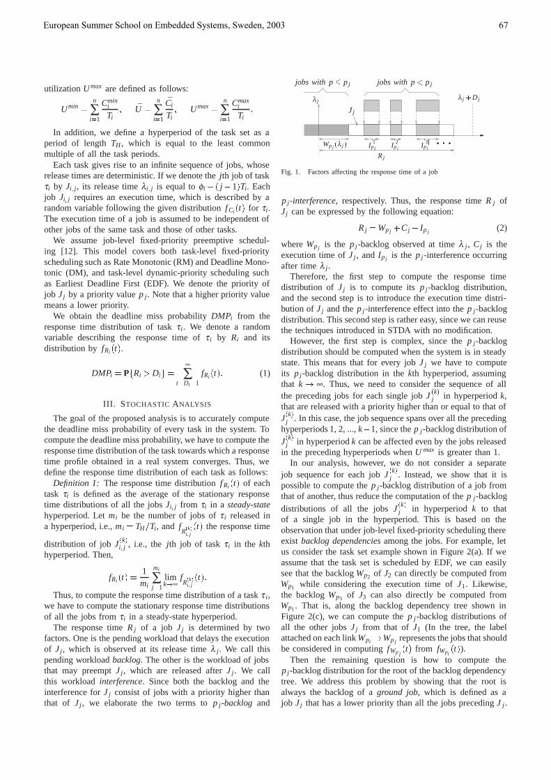
utilization Umax are defined as follows:
Uminn
∑i1
Cmini
Ti U
n
∑i1
Ci
Ti Umax
n
∑i1
Cmaxi
Ti
In addition, we define a hyperperiod of the task set as aperiod of lengthTH , which is equal to the least commonmultiple of all the task periods.
Each task gives rise to an infinite sequence of jobs, whoserelease times are deterministic. If we denote thejth job of taskτi by Ji j , its release timeλi j is equal toφi j1Ti. Eachjob Ji j requires an execution time, which is described by arandom variable following the given distributionfCi t for τi .The execution time of a job is assumed to be independent ofother jobs of the same task and those of other tasks.
We assume job-level fixed-priority preemptive schedul-ing [12]. This model covers both task-level fixed-priorityscheduling such as Rate Monotonic (RM) and Deadline Mono-tonic (DM), and task-level dynamic-priority scheduling suchas Earliest Deadline First (EDF). We denote the priority ofjob Jj by a priority valuep j . Note that a higher priority valuemeans a lower priority.
We obtain the deadline miss probabilityDMPi from theresponse time distribution of taskτ i . We denote a randomvariable describing the response time ofτ i by Ri and itsdistribution by fRi t.
DMPi PRi Di∞
∑tDi1
fRi t (1)
III. STOCHASTIC ANALYSIS
The goal of the proposed analysis is to accurately computethe deadline miss probability of every task in the system. Tocompute the deadline miss probability, we have to compute theresponse time distribution of the task towards which a responsetime profile obtained in a real system converges. Thus, wedefine the response time distribution of each task as follows:
Definition 1: The response time distributionfRi t of eachtask τi is defined as the average of the stationary responsetime distributions of all the jobsJi j from τi in a steady-statehyperperiod. Letmi be the number of jobs ofτ i released ina hyperperiod, i.e.,mi THTi , and f
Rki jt the response time
distribution of jobJki j , i.e., the jth job of taskτi in the kthhyperperiod. Then,
fRi t 1mi
mi
∑j1
limk∞
fRk
i jt
Thus, to compute the response time distribution of a taskτ i ,we have to compute the stationary response time distributionsof all the jobs fromτi in a steady-state hyperperiod.
The response timeRj of a job Jj is determined by twofactors. One is the pending workload that delays the executionof Jj , which is observed at its release timeλ j . We call thispending workloadbacklog. The other is the workload of jobsthat may preemptJj , which are released afterJj . We callthis workload interference. Since both the backlog and theinterference forJj consist of jobs with a priority higher thanthat of Jj , we elaborate the two terms topj-backlog and
Wpj λ j I 1pj I 2
pj I 3pj
Rj
jobs with p pj jobs with p pj
λ j Dj
λ j
Jj
Fig. 1. Factors affecting the response time of a job
pj-interference, respectively. Thus, the response timeRj ofJj can be expressed by the following equation:
Rj Wpj Cj Ipj (2)
whereWpj is the pj -backlog observed at timeλ j , Cj is theexecution time ofJj , and I pj is the pj -interference occurringafter timeλ j .
Therefore, the first step to compute the response timedistribution of Jj is to compute itspj -backlog distribution,and the second step is to introduce the execution time distri-bution ofJj and thepj -interference effect into thep j -backlogdistribution. This second step is rather easy, since we can reusethe techniques introduced in STDA with no modification.
However, the first step is complex, since thep j -backlogdistribution should be computed when the system is in steadystate. This means that for every jobJj we have to computeits pj -backlog distribution in thekth hyperperiod, assumingthat k ∞. Thus, we need to consider the sequence of allthe preceding jobs for each single jobJkj in hyperperiodk,that are released with a priority higher than or equal to that ofJkj . In this case, the job sequence spans over all the precedinghyperperiods 1, 2, ...,k1, since thep j -backlog distribution ofJkj in hyperperiodk can be affected even by the jobs releasedin the preceding hyperperiods whenU max is greater than 1.
In our analysis, however, we do not consider a separatejob sequence for each jobJkj . Instead, we show that it ispossible to compute thepj -backlog distribution of a job fromthat of another, thus reduce the computation of thep j -backlog
distributions of all the jobsJkj in hyperperiodk to thatof a single job in the hyperperiod. This is based on theobservation that under job-level fixed-priority scheduling thereexist backlog dependenciesamong the jobs. For example, letus consider the task set example shown in Figure 2(a). If weassume that the task set is scheduled by EDF, we can easilysee that the backlogWp2 of J2 can directly be computed fromWp1 while considering the execution time ofJ1. Likewise,the backlogWp3 of J3 can also directly be computed fromWp1. That is, along the backlog dependency tree shown inFigure 2(c), we can compute thep j -backlog distributions ofall the other jobsJj from that of J1 (In the tree, the labelattached on each linkWpi Wpj represents the jobs that shouldbe considered in computingfWpj
t from fWpit).
Then the remaining question is how to compute thepj -backlog distribution for the root of the backlog dependencytree. We address this problem by showing that the root isalways the backlog of aground job, which is defined as ajob Jj that has a lower priority than all the jobs precedingJ j .
European Summer School on Embedded Systems, Sweden, 2003 67

0 70 140
0 20 40 60 80 100 120 140
J8 J9
Wp10
Wp11
J10 J11
J8
J9
Wp6Wp4
Wp1
Wp8
Wp9
Wp2
Wp5 Wp7Wp3
Wp5
Wp1
Wp3
Wp4
Wp2
Wp6
Wp9
Wp7
Wp8
J1J3
J1
J5J7
J5
J1
J2J3J4
J5
J6J7J8
(b) Ground jobs and non-ground jobs (c) Backlog dependency tree
(a) Task set
τ1
τ2 J2
J1 J7J5J4J3
J6
hyperperiod
J1
J3 J4
J5
J7
J2 J6
Fig. 2. An example of backlog dependency tree generation
This means that thepj -backlog of such a job is always equalto the total backlog in the system observed at the same time,called system backlog W, and thus it is possible to computeits stationary distribution by Markov process modeling. Thatis, we prove that the evoluation of the system backlog overhyperperiodsW1
W2 Wk
as a Markov process,derive a set of equilibrium equations, and solve them.
Therefore, the proposed analysis is summarized into thefollowing three steps: 1) compute the stationary system back-log distribution of a ground job by Markov process modeling(steady-state system backlog analysis), 2) compute the sta-tionary pj -backlog distributions of all the other jobs usingbacklog dependencies (p j-backlog analysis), and 3) constructthe stationary response time distributions of all the jobs byintroducing into each stationaryp j -backlog distribution theexecution time distribution of the jobJ j and thepj -interferenceeffect (pj -interference analysis). For more details on thesethree steps, refer to [13].
IV. EXPERIMENTAL RESULTS
To evaluate the sensitivity of the proposed analysis tothe system utilization, we use five task sets with differentutilization values, as shown in Table I. All the task sets consistof three tasks with the same periods, the same deadlines, andnull phases, thus result in the same backlog dependency treefor any scheduling algorithm.
Table I summarizes the results of our analysis, includingthe results obtained by STDA for the case of RM. Thistable shows the deadline miss probability (DMP) for eachtask and the average deadline miss ratio (DMR) and standarddeviation obtained from simulations. The average DMR isobtained by averaging the deadline miss ratios measured from100 simulation runs of each task set, performed during 5000hyperperiods.
From Table I, we can see that our analysis results are almostidentical to the simulation results. For the case of STDA,however, the analysis results get worse asU or Umax increases.In the case ofτ3 in task setA, the DMP given by STDA
(39.3%) is more than four times the DMP given by our analysis(9.4%).
V. CONCLUSIONS ANDFUTURE WORK
In this paper we have proposed a stochastic analysis toaccurately compute the response time distributions of tasksfor general priority-driven periodic real-time systems. Theproposed analysis can be uniformly applied to general priority-driven system including both fixed-priority systems such asRM and DM, and dynamic-priority systems such as EDF,thanks to the backlog dependency relations among all thejobs in a hyperperiod. The experimental results have shownthat our analysis is highly accurate regardless of the systemutilization, while STDA is not. For future work, it should beaddressed how to reduce the computational complexity of theanalysis, which is known asOn3m3 (n: the number of jobsin a hyperperiod,m: the maximum length of the executiontime distributions), and whether it is possible to safely analyzetasks that have variable interrelease times with our analysis bymodeling them as periodic tasks.
ACKNOWLEDGMENT
The authors would like to thank Prof. Jane Liu for hervaluable comments and suggestions for the extension of theproposed analysis.
REFERENCES
[1] L. Liu and J. Layland, “Scheduling Algorithms for Multiprogrammingin a Hard Real-Time Environment,”Journal of ACM, vol. 20, no. 1, pp.46–61, 1973.
[2] J. P. Lehoczky, L. Sha, and Y. Ding, “The Rate-Monotonic SchedulingAlgorithm: Exact Characterization and Average Case Behavior,” inProc.of the 10th IEEE Real-Time Systems Symposium, Dec. 1989.
[3] J. P. Lehoczky, “Fixed Priority Scheduling of Periodic Task Sets withArbitrary Deadlines,” inProc. of the 11th IEEE Real-Time SystemsSymposium, Dec. 1990, pp. 201–209.
[4] M. K. Gardner and J. W. Liu, “Analyzing Stochastic Fixed-Priority Real-Time Systems,” inProc. of the 5th International Conference on Toolsand Algorithms for the Construction and Analysis of Systems, Mar. 1999.
European Summer School on Embedded Systems, Sweden, 2003 68

task set Ti Di
execution times utilizations RM EDFCmin
i Ci Cmaxi Umin U Umax simulation STDA our analysis simulation our analysis
Aτ1 20 20 4 6 10
.58 .82 1.27.0000 .0000 .0000 .0000 .0001 .0000 .0001
τ2 60 60 12 16 22 .0000 .0000 .0000 .0000 .0000 .0000 .0000τ3 90 90 16 23 36 .0940 .0025 .3931 .0940 .0000 .0000 .0000
Bτ1 20 20 4 6 10
.58 .87 1.27.0000 .0000 .0000 .0000 .0013 .0002 .0013
τ2 60 60 12 17 22 .0000 .0000 .0000 .0000 .0005 .0002 .0005τ3 90 90 16 26 36 .2173 .0033 .6913 .2170 .0000 .0001 .0000
Cτ1 20 20 4 7 10
.58 .92 1.27.0000 .0000 .0000 .0000 .0223 .0013 .0224
τ2 60 60 12 17 22 .0000 .0000 .0000 .0000 .0168 .0014 .0169τ3 90 90 16 26 36 .3849 .0052 .9075 .3852 .0081 .0011 .0081
C1τ1 20 20 3 7 11
.46 .92 1.38.0000 .0000 .0000 .0000 .0626 .0031 .0627
τ2 60 60 10 17 24 .0000 .0000 .0000 .0000 .0604 .0038 .0607τ3 90 90 13 26 39 .4332 .0065 .9209 .4334 .0461 .0032 .0463
C2τ1 20 20 2 7 12
.34 .92 1.50.0000 .0000 .0000 .0000 .1248 .0058 .1250
τ2 60 60 8 17 26 .0002 .0001 .0018 .0002 .1293 .0064 .1296τ3 90 90 10 26 42 .4859 .0081 .9339 .4860 .1136 .0063 .1138
TABLE I
COMPARISON BETWEEN THE SIMULATION AND THE ANALYSIS
[5] J. P. Lehoczky, “Real-Time Queueing Theory,” inProc. of the 17th IEEEReal-Time Systems Symposium, Dec. 1996, pp. 186–195.
[6] ——, “Real-Time Queueing Network Theory,” inProc. of the 18th IEEEReal-Time Systems Symposium, Dec. 1997, pp. 58–67.
[7] L. Abeni and G. Buttazzo, “Stochastic Analysis of a Reservation BasedSystem,” in Proc. of the 9th International Workshop on Parallel andDistributed Real-Time Systems, Apr. 2001.
[8] A. K. Atlas and A. Bestavros, “Statistical Rate Monotonic Scheduling,”in Proc. of the 19th IEEE Real-Time Systems Symposium, Dec. 1998,pp. 123–132.
[9] J. Leung and J. Whitehead, “On the Complexity of Fixed PriorityScheduling of Periodic Real-Time Tasks,”Performance Evaluation,vol. 2, no. 4, pp. 237–250, 1982.
[10] A. Terrasa and G. Bernat, “Extracting Temporal Properties from Real-Time Systems by Automatic Tracing Analysis,” inProc. of the 9th Inter-national Conference on Real-Time and Embedded Computing Systemsand Applications, Feb. 2003.
[11] G. Bernat, A. Colin, and S. Petters, “WCET Analysis of ProbabilisticHard Real-Time Systems,” inProc. of the 23rd IEEE Real-Time SystemsSymposium, Dec. 2002.
[12] J. W. S. Liu,Real-Time Systems. Prentice Hall, 2000.[13] J. L. Dıaz, D. F. Garc´ıa, K. Kim, C.-G. Lee, L. LoBello, J. M. L´opez,
S. L. Min, and O. Mirabella, “Stochastic Analysis of Periodic Real-TimeSystems,” inProc. of the 23rd Real-Time Systems Symposium, Austin,TX, USA, Dec. 2002, pp. 289–300.
Kanghee Kim received the BS, MS, and PhD degrees in computer engineeringfrom Seoul National University, Seoul, Korea in 1996, 1998, and 2004,respectively. He is currently working with LG Electronics Co., Ltd. in Korea.His current research interests are in real-time system design and analysis.
Jose Luis Dıaz received the BSc and PhD degrees in electrical engineeringfrom the University of Oviedo, Gij´on, Spain, in 1990 and 2003, respectively.He is currently an Associate Professor in the Department of Computer Science,the University of Oviedo. He was granted a scholarship in 1991, and sincethen he has been working in industrial applications of parallel processingand computer vision. His current research interests are in real-time systemanalysis.
Lucia Lo Bello was awarded the Laurea degree in electronic engineeringin 1994 and the PhD degree in computer science and electronic engineeringin 1998, both by the University of Catania, Italy. During the academic year2000-2001 she was a Visiting Researcher in the Department of ComputerEngineering of Seoul National University, Seoul, Korea. She is currently anAssistant Professor with tenure in the Department of Computer Science andTelecommunications at the University of Catania. She has served on a numberof program committees of technical conferences and workshops in the areasof real-time systems and factory communication. She is also a reviewer fora number of international journals. Her research interests include real-timesystem design, real-time scheduling, stochastic analysis of real-time systems,distributed real-time systems, real-time networks, factory communication andembedded systems. Dr. Lo Bello is a member of the IEEE Computer Society.
Jose Marıa Lopezreceived the BSc and PhD degrees in electrical engineeringfrom the University of Oviedo, Gij´on, Spain, in 1993 and 2002, respectively.He was granted a scholarship in 1994, and since then he has been working inapplications of high performance computing for the steel industry. Currently,he is an Assistant Professor of computer architecture at the University ofOviedo. His current research interests are in signal processing, real-timecomputing and scheduling algorithms.
Chang-Gun Lee received the BS, MS and PhD degrees in computer en-gineering from Seoul National University, Seoul, Korea, in 1991, 1993 and1998, respectively. He is currently an Assistant Professor in the Department ofElectrical Engineering, Ohio State University, Columbus. Previously, he wasa Research Scientist in the Department of Computer Science, University ofIllinois at Urbana-Champaign from March 2002 to July 2002 and a ResearchEngineer in the Advanced Telecomm. Research Lab., LG Information &Communications, Ltd. from March 1998 to February 2000. His currentresearch interests include real-time systems, complex embedded systems, QoSmanagement, and mobile communications. Dr. Lee is a member of the IEEEComputer Society.
Daniel F. Garcıa is a Professor at the Department of Computer Scienceat Oviedo University. In 1988, he received the PhD degree in electricalengineering from Oviedo University. Since 1994 he has been responsiblefor the computer engineering area at the University of Oviedo. His currentresearch interests are in the area of the development of high performancereal-time and embedded systems applied to quality assurance and productioninspection in industry. For the last ten years, Dr. Garcia has been conductingresearch projects in the area of information technologies applied to industryat national and European levels. He is a member of ACM and the IEEEComputer Society.
Sang Lyul Min received the BS and MS degrees in computer engineering,both from Seoul National University, Seoul, Korea, in 1983 and 1985,respectively. In 1985, he was awarded a Fullbright scholarship to pursuefurther graduate studies at the University of Washington. He received the MSand PhD degrees in computer science from the University of Washington,Seattle, in 1988 and 1989, respectively. He is currently a Professor in theSchool of Computer Science and Engineering, Seoul National University,Seoul, Korea. He has served on a number of program committees of technicalconferences and workshops, including the IEEE Real-Time Systems Sympo-sium (RTSS), the IEEE Real-Time Technology and Applications Symposium(RTAS), the ACM SIGPLAN Workshop on Languages, Compilers, andTools for Embedded Systems (LCTES), and the International Conference onDistributed Computing Systems (ICDCS). He is also a member of the editorialboard of the IEEE Transactions on Computers. His research interests includecomputer architecture, real-time computing, parallel processing, and computerperformance evaluation. Dr. Min is a member of the IEEE Computer Society.
Orazio Mirabella was awarded the Laurea degree in physics in 1971, bythe University of Catania, Italy. Since 1987 he has been at the engineeringfaculty, the University of Catania and is currently a Professor of computernetworks. In the years from 1982 to 2001 he was a member of Sub CommitteeSC65C of International Electrotechnical Commission (IEC), contributing tothe definition of several international standards. His research interests includeperformance evaluation of networks for process control, real-time systemdesign, distributed real-time systems, and embedded systems.
European Summer School on Embedded Systems, Sweden, 2003 69
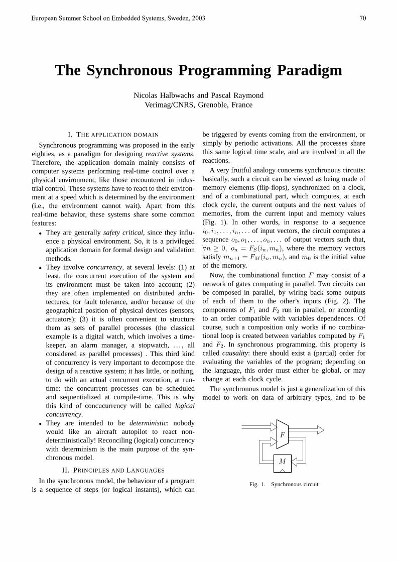
The Synchronous Programming Paradigm
Nicolas Halbwachs and Pascal RaymondVerimag/CNRS, Grenoble, France
I. THE APPLICATION DOMAIN
Synchronous programming was proposed in the earlyeighties, as a paradigm for designing reactive systems.Therefore, the application domain mainly consists ofcomputer systems performing real-time control over aphysical environment, like those encountered in indus-trial control. These systems have to react to their environ-ment at a speed which is determined by the environment(i.e., the environment cannot wait). Apart from thisreal-time behavior, these systems share some commonfeatures:
• They are generally safety critical, since they influ-ence a physical environment. So, it is a privilegedapplication domain for formal design and validationmethods.
• They involve concurrency, at several levels: (1) atleast, the concurrent execution of the system andits environment must be taken into account; (2)they are often implemented on distributed archi-tectures, for fault tolerance, and/or because of thegeographical position of physical devices (sensors,actuators); (3) it is often convenient to structurethem as sets of parallel processes (the classicalexample is a digital watch, which involves a time-keeper, an alarm manager, a stopwatch, . . . , allconsidered as parallel processes) . This third kindof concurrency is very important to decompose thedesign of a reactive system; it has little, or nothing,to do with an actual concurrent execution, at run-time: the concurrent processes can be scheduledand sequentialized at compile-time. This is whythis kind of concucurrency will be called logicalconcurrency.
• They are intended to be deterministic: nobodywould like an aircraft autopilot to react non-deterministically! Reconciling (logical) concurrencywith determinism is the main purpose of the syn-chronous model.
II. PRINCIPLES AND LANGUAGES
In the synchronous model, the behaviour of a programis a sequence of steps (or logical instants), which can
be triggered by events coming from the environment, orsimply by periodic activations. All the processes sharethis same logical time scale, and are involved in all thereactions.
A very fruitful analogy concerns synchronous circuits:basically, such a circuit can be viewed as being made ofmemory elements (flip-flops), synchronized on a clock,and of a combinational part, which computes, at eachclock cycle, the current outputs and the next values ofmemories, from the current input and memory values(Fig. 1). In other words, in response to a sequencei0, i1, . . . , in, . . . of input vectors, the circuit computes asequence o0, o1, . . . , on, . . . of output vectors such that,∀n ≥ 0, on = FS(in,mn), where the memory vectorssatisfy mn+1 = FM (in,mn), and m0 is the initial valueof the memory.
Now, the combinational function F may consist of anetwork of gates computing in parallel. Two circuits canbe composed in parallel, by wiring back some outputsof each of them to the other’s inputs (Fig. 2). Thecomponents of F1 and F2 run in parallel, or accordingto an order compatible with variables dependences. Ofcourse, such a composition only works if no combina-tional loop is created between variables computed by F1
and F2. In synchronous programming, this property iscalled causality: there should exist a (partial) order forevaluating the variables of the program; depending onthe language, this order must either be global, or maychange at each clock cycle.
The synchronous model is just a generalization of thismodel to work on data of arbitrary types, and to be
F
M
Fig. 1. Synchronous circuit
European Summer School on Embedded Systems, Sweden, 2003 70

M1
F2
M2
F1
Fig. 2. Synchronous composition
used not only for hardware but also for software. Theconnection between synchronous programming and thecircuit model is more or less apparent, depending of thestyle of the language used:
• The similarity is obvious for data-flow languages, likeLustre [1] or Signal [2]. In these languages, a programcan be viewed as a generalized circuit. As a matter offact, the “circuit” of Fig. 1 would be described in Lustreby the following equation:
(O,M) = F(I, M0 -> pre(M))
which expresses that, at each instant (clock cycle),the values of the outputs O and the memories M arethe results of the combinational function F applied tocurrent inputs I and to previous values of the memory(pre(M)), initialized with M0.
• In imperative languages like Esterel [3], [4] or Sync-chart [5], the underlying circuit model is less evident. Itis more natural to consider a program as a synchronouscomposition of automata, which may be hierarchic (inthe sense that a “state” of an automaton can be “refined”by a sub-automaton). Such a program is compiled intoa generalized circuit as before. For instance, the classi-cal “timekeeper” program, where a first process counts“seconds” to emit “minutes” towards an other processcounting “minutes” to emit “hours”, etc., can be writtenas follows in Esterel:
[every 60 SECOND do emit MINUTE end
||every 60 MINUTE do emit HOUR end
]
and behaves exactly as written: in the same logicalinstant where the 60th SECOND happens, the MINUTEsignal is emitted, and perceived by all processes whichare “listening” to it, and in particular by the one whichtakes care of HOURs, the counter of which is incre-mented in the very same reaction. This program canalso be viewed as the synchronous product of two inter-preted automata (Fig. 3). Logical instants correspond to,possibly simultaneous, firings of transitions: every sixtySECONDs, the former automaton emits a MINUTEsignal, which triggers a transition of the later automaton.
s:=0
SECOND ?s=59 ?
s:=0emit MINUTE
SECOND ?s < 59 ?s++
m:=0
MINUTE ?m=59 ?
m:=0emit HOUR
MINUTE ?m < 59 ?m++
SECOND ?s < 59 ?
s++
SECOND ?s=59 ?
emit MINUTE
SECOND ?s=59 ?m=59 ?emit MINUTEs:=m:=0emit HOUR
s:=m:=0
m < 59 ?
s:=0m++
Fig. 3. Synchronous counters and their product
III. IMPORTANT TOPICS AND ONGOING RESEARCH
This section briefly reviews the main topics specificto the synchronous model, and the current trends of
European Summer School on Embedded Systems, Sweden, 2003 71

research.a) Semantics issues: One of the main features of
synchronous languages is their completely formal andclean semantics. In particular, the timing behaviour ofprograms is perfectly determined with respect to thelogical time scale. We already mentioned the semanticproblem of causality, which is specific to synchronouslanguages: One can write programs with combinationalloops, which don’t make sense in general, but aresometimes difficult to detect. This question, which isnow completely solved [6], originated most problemsof “almost synchronous” formalisms, like Statecharts orSequential Function Charts.
b) Compilation: Most efforts were devoted to se-quential code generation. Two main solutions were ex-plored, together with intermediate versions: the compila-tion into an explicit automaton — which produces veryefficient code, but often involves an explosion of the codesize — and the translation into a single loop — “readinputs / compute outputs / update memories”. Gener-ating code for distributed architectures is much moredifficult [7], [8] and still concerns ongoing research.Compiling synchronous languages into circuits is alsoan important topic [9], [10]
c) Verification: Program verification is of coursean important goal for reactive systems. The synchronousmodel enjoys a very nice feature in this domain: pro-grams, called synchronous observers, can be used toexpress safety properties of other programs. Such anobserver is a program taking as inputs the signalsor variables which are relevant for the property, andemitting an “alarm” whenever the property is violated.They are used both for expressing desired properties ofprograms, and assumptions about their environment (fora property is rarely satisfied independently of any knowl-edge about the environment). The verification goal isthen to establish that, when considering the combinationof the program and its two observers (Fig. 4), if theassumption observer never complains, neither does theproperty observer. Such a verification can be performedusing standard model-checking techniques (possibly us-ing abstraction) [11], [12], [13], or abstract interpretation[14]. Program testing is also an important topic [15]which can benefit from the technique of synchronousobservers.
d) Language issues: Synchronous languages arestill under development. Trends are to introduce asyn-chronous concepts [16], [17], and to combine imperativeand data-flow concepts [18]: now, Esterel-V7 integratesEsterel and Lustre.
incorrect
unrealistic
property
observer
observer
assumption
verificationunder
program
Fig. 4. Synchronous observers
IV. BIBLIOGRAPHY
There is no room, here, for an exhaustive bibli-ography on the domain of synchronous programming.However, most references can be found from a few basicbooks [19], [3] and articles [20], [21], [22].
REFERENCES
[1] N. Halbwachs, P. Caspi, P. Raymond, and D. Pilaud, “Thesynchronous dataflow programming language LUSTRE,” Pro-ceedings of the IEEE, vol. 79, no. 9, pp. 1305–1320, Sept. 1991.
[2] P. LeGuernic, T. Gautier, M. LeBorgne, and C. LeMaire, “Pro-gramming real time applications with SIGNAL,” Proceedings ofthe IEEE, vol. 79, no. 9, pp. 1321–1336, Sept. 1991.
[3] G. Berry, “The constructive semantics of esterel,” 1995,draft book available by ftp at ftp-sop.inria.fr/meije/esterel/papers/constructiveness.ps.gz.
[4] F. Boussinot and R. Simone, “The ESTEREL language,” Pro-ceedings of the IEEE, vol. 79, no. 9, pp. 1293–1304, Sept. 1991.
[5] C. Andre, “Representation and analysis of reactive behaviors:a synchronous approach,” in IEEE-SMC’96, ComputationalEngineering in Systems Applications, Lille, France, July 1996.
[6] T. R. Shiple, G. Berry, and H. Touati, “Constructive analysis ofcyclic circuits,” in International Design and Testing ConferenceIDTC’96, Paris, France, 1996.
[7] P. Caspi, A. Girault, and D. Pilaud, “Distributing reactivesystems,” in Seventh International Conference on Parallel andDistributed Computing Systems, PDCS’94. Las Vegas, USA:ISCA, Oct. 1994.
[8] A. Benveniste, P. Caspi, and S. Tripakis, “Distributing syn-chronous programs on a loosely synchronous, distributed ar-chitecture,” Irisa, Research Report 1289, Dec. 1999.
[9] G. Berry, “Esterel on hardware,” Philosophical TransactionsRoyal Society of London, vol. 339, pp. 217—248, 1992.
[10] A. Kountouris and C. Wolinski, “A method for the generationof hdl code at the rtl level form a high-level formal specificationlanguage,” in Proceedings of MWSCAS’97. Sacramento: IEEEComputer Society Press, Aug. 1997.
[11] N. Halbwachs, F. Lagnier, and C. Ratel, “Programming andverifying real-time systems by means of the synchronous data-flow programming language LUSTRE,” IEEE Transactions onSoftware Engineering, Special Issue on the Specification andAnalysis of Real-Time Systems, pp. 785–793, Sept. 1992.
[12] M. Le Borgne, B. Dutertre, A. Benveniste, and P. Le Guernic,“Dynamical systems over Galois fields,” in European ControlConference, Groningen, 1993, pp. 2191–2196.
European Summer School on Embedded Systems, Sweden, 2003 72
[13] A. Bouali, “Xeve: an Esterel verification environment,” inTenth International Conference on Computer-Aided Verification,CAV’98. Vancouver (B.C.): LNCS 1427, Springer Verlag, June1998.
[14] N. Halbwachs, Y. Proy, and P. Roumanoff, “Verification of real-time systems using linear relation analysis,” Formal Methods inSystem Design, vol. 11, no. 2, pp. 157–185, Aug. 1997.
[15] P. Raymond, D. Weber, X. Nicollin, and N. Halbwachs, “Au-tomatic testing of reactive systems,” in 19th IEEE Real-TimeSystems Symposium, Madrid, Spain, Dec. 1998.
[16] G. Berry and E. Sentovich, “Multiclock esterel,” in CorrectHardware Design and Verification Methods, CHARME’01.Livingston (Scotland): LNCS 2144, Springer Verlag, Sept.2001.
[17] A. Benveniste, B. Caillaud, and P. L. Guernic, “From synchronyto asynchrony,” in CONCUR’99, J. Baeten and S. Mauw, Eds.LNCS 1664, Springer Verlag, 1999.
[18] F. Maraninchi and Y. Remond, “Mode-automata: About modesand states for reactive systems,” in European Symposium OnProgramming. Lisbon (Portugal): Springer Verlag, Mar. 1998.
[19] N. Halbwachs, Synchronous programming of reactive systems.Kluwer Academic Pub., 1993.
[20] “Another look at real-time programming,” Special Section ofthe Proceedings of the IEEE, vol. 79, no. 9, Sept. 1991.
[21] N. Halbwachs, “Synchronous programming of reactive systems,a tutorial and commented bibliography,” in Tenth InternationalConference on Computer-Aided Verification, CAV’98. Vancou-ver (B.C.): LNCS 1427, Springer Verlag, June 1998.
[22] A. Benveniste, P. Caspi, S. Edwards, N. Halbwachs, P. LeGuernic, and R. de Simone, “The synchronous languages 12years later,” Proceedings of the IEEE, vol. 91, no. 1, Jan. 2003.
European Summer School on Embedded Systems, Sweden, 2003 73
Formal Methods for Schedulability and PerformanceAnalysis of Real-Time Embedded Systems
Insup Lee, Anna Philippou
, Oleg Sokolsky
Department of Computer and Information ScienceUniversity of Pennsylvania
Philadelphia, PA 19104Email: lee,sokolsky @cis.upenn.edu
Department of Computer and Information ScienceUniversity of Cyprus
Nicosia, CyprusEmail: [email protected]
I. MOTIVATION
Reliability in real-time systems can be improved throughthe use of formal methods for the specification and analysis oftimed behaviors. Recently, there has been a spate of progressin the development of real-time formal methods. Much ofthis work falls into the traditional categories of untimedsystems such as temporal logics, assertional methods, net-based models, automata theory and process algebras. In thispaper, we provide an overview of the family of resource-boundreal-time process algebras that we have developed.
Process algebras, such as CCS [8], CSP [5], AcceptanceTrees [4] and ACP [2], have been developed to describe andanalyze communicating, concurrently executing systems. Theyare based on the premises that the two most essential notionsin understanding complex dynamic systems are concurrencyand communication [8]. The most salient aspect of processalgebras is that they support the modular specification andverification of a system. This is due to the algebraic lawsthat form a compositional proof system which enables theverification of a whole system by reasoning about its parts.Process algebras are being used widely in specifying andverifying concurrent systems.
Algebra of Communicating Shared Resource (ACSR) intro-duced by Lee et. al. [7], is a timed process algebra whichcan be regarded as an extension of CCS. The timing behaviorof a real-time system depends not only on delays due toprocess synchronization, but also on the availability of sharedresources. Most current real-time process algebras adequatelycapture delays due to process synchronization; however, theyabstract out resource-specific details by assuming idealisticoperating environments. On the other hand, scheduling andresource allocation algorithms used for real-time systemsignore the effect of process synchronization except for simpleprecedence relations between processes. ACSR algebra pro-vides a formal framework that combines the areas of processalgebra and real-time scheduling, and thus, can help us toreason about systems that are sensitive to deadlines, process
This research was supported in part by NSF CCR-9988409, NSF CCR-0086147, NSF CCR-0209024 and ARO DAAD19-01-1-0473
interaction and resource availability.ACSR supports the notions of resources, priorities, interrupt,
timeout, and process structure. The notion of real-time inACSR is quantitative and discrete, and is accommodated usingthe concept of timed actions. Executing a timed action requiresaccess to a set of resources and takes one unit of time.Resources are serially reusable, and access to them is governedby priorities. Similar to CCS, the execution of an event isinstantaneous and never consumes any resource. The notion ofcommunication is modeled using events through the executionof complementary events, which are then converted into aninternal event. As with timed actions, priorities are also usedto arbitrate the choice of several events that are possible atthe same time. Although the concurrency model of CCS-likeprocess algebras is based on interleaving semantics, ACSRincludes interleaving semantics for events as well as lock-stepparallelism for timed actions.
The computation model of ACSR is based on the view that areal-time system consists of a set of communicating processesthat use shared resources for execution and synchronize withone another. The use of shared resources is represented bytimed actions and synchronization is supported by instanta-neous events. The execution of a timed action is assumed totake one time unit and to consume a set of resources duringthe same time unit. Idling of a process is treated as a specialtimed action that consumes no resources. The execution of atimed action is subject to availability of the resources usedin the timed action. The contention for resources is arbitratedaccording to the priorities of competing actions. To ensure theuniform progression of time, processes execute timed actionssynchronously. Unlike a timed action, the execution of an eventis instantaneous and never consumes any resource. Processesexecute events asynchronously except when two processessynchronize through matching events. Priorities are used todirect the choice when several events are possible at the sametime.
We have extended ACSR into a family of process algebras,GCSR [1], Dense-time ACSR [3], ACSR-VP [6], PACSR [9]and P ACSR [10]. GCSR is a graphical version of ACSRwhich allows the visual representation of ACSR processes.
European Summer School on Embedded Systems, Sweden, 2003 74

Dense-time ACSR is an extension of ACSR with dense time.ACSR-VP extends ACSR with value-passing capability so thatarbitrary scheduling problems can be specified and analyzed.PACSR (Probabilistic ACSR) allows the modeling of resourcefailure with probabilities, whereas P ACSR extends PACSRwith the notion of power consumption and resource constraintsof embedded systems.
II. BACKGROUND: THE COMPUTATION MODEL
In our algebra there are two types of actions: those whichconsume time, and those which are instantaneous. The time-consuming actions represent one “tick” of a global clock.These actions may also represent the consumption of re-sources, e.g., CPUs, devices, memory, batteries in the systemconfiguration. In contrast, the instantaneous actions providea synchronization mechanism between a set of concurrentprocesses.
Timed Actions. We consider a system to be composed ofa finite set of serially reusable resources, denoted by . Anaction that consumes one “tick” of time is drawn from thedomain , with the restriction that each resource berepresented at most once. As an example, the singleton action, , denotes the use of some resource running atthe priority level . The action represents idling for one timeunit, since no resuable resource is consumed.
We use to denote the domain of timed actions, and welet ! range over . We define " to be the set ofresources used by the action ; e.g., " ' ' + ' . We also use - / to denote the priority level of theuse of resource in action ; e.g., - / 2 ' ' +
' . By convention, if is not in " , then - / + 5 .Instantaneous Events. We call instantaneous actions
events, which provide the basic synchronization in our processalgebra. We assume a set of channels 6 . An event is denotedby a pair 7 , where 7 is the label of the event, and is itspriority. Labels are drawn from the set 8 : <8 : ? , wherefor all 7 6 7 D 8 and 7 F <8 . We say that 7 D and 7 F areinverse labels. As in CCS, the special identity label,
?, arises
when two events with inverse labels are executed in parallel.We use I to denote the domain of events, and let J , K andL range over I . We use M J and - J to represent the label
and priority, respectively, of the event J . The entire domain ofactions is + : I , and we let R and S range over .
The executions of a process are defined by a timed labeledtransition system (timed LTS). A timed LTS T is defined asU W [ ] , where (1)
Wis a set of ACSR processes, ranged
over by ^ ` , (2) is a set of actions, and (3) [ is a labeledtransition relation such that ^ ab b b b [ ` if the process ^may perform an instantaneous event or timed action R andthen behave as ` .
For example, a process ^ ' may have the following behavior:^ ' a 2b b b b [ ^ a hb b b b [ ^ k a lb b b b [ n n n That is, ^ ' first executesR ' and evolves into ^ , which executes R , etc. It takesno time to execute an instantaneous event. A timed actionhowever is executed for exactly one unit of time.
III. A FAMILY OF RESOURCE-BOUND REAL-TIME
PROCESSES
We briefly describe four process algebras: ACSR, PACSR,ACSR-VP and P ACSR.
A. Real-Time Processes
The following grammar describes the syntax of ACSRprocesses.
^ o o + r t u w 7 y n ^ w o ^ w ^ | ^ w ^ ^ w^ ^ ^ ^ w ^ w ^ w ^ w [ ^ w ! n
The process r t u represents the inactive process. There aretwo prefix operators, corresponding to the two types of actions.The process 7 y n ^ executes the instantaneous event 7 y and proceeds to ^ . The process o ^ executes a resource-consuming action during the first time unit and proceeds to
^ . The process ^ | ` represents a nondeterministic choicebetween the two summands. The process ^ ` describes theconcurrent composition of ^ and ` : the component processesmay proceed independently or interact with one another whileexecuting events, and they synchronize on timed actions.
The scope construct, ^ ` , binds the process ^by a temporal scope and incorporates the notions of timeoutand interrupts. We call the time bound, where : and require that ^ may execute for a maximum of timeunits. The scope may be exited in one of three ways: First, if
^ terminates successfully within time-units by executing anevent labeled 7 F where 7 6 , then control is delegated to ` ,the success-handler. Else, if ^ fails to terminate within time then control proceeds to . Finally, throughout execution ofthis process construct, ^ may be interrupted by process .
In ^ , where 6 , the scope of channels in isrestricted to process ^ , and thus, components of ^ may usethese labels to interact with one another but not with ^ ’senvironment. The construct ^ , , produces a processthat reserves the use of resources in for itself, extendingevery action in ^ with resources in b " at priority0. ^ hides the identity of resources in so that they arenot visible on the interface with the environment. That is, theoperator ^ binds all free occurrences of the resources of
in ^ . This binder gives rise to the sets of free and boundresources of a process ^ . Process [ ^ represents theconditional process: it performs as ^ if boolean expression evaluates to true and as r t u otherwise. Process constant !with process definition ! + ^ allows standard recursion.
B. Resource Probabilities and Actions
PACSR (Probabilistic ACSR) extends the process algebraACSR by associating with each resource a probability. Thisprobability captures the rate at which the resource may fail.Since instantaneous events in PACSR are identical to those ofACSR, we only discuss timed actions, which now can accountfor resource failure.
Timed Actions. As in ACSR, we assume that a systemcontains a finite set of serially reusable resources drawn fromthe set . We also consider set that contains, for each , an element , representing the failed resource . We
European Summer School on Embedded Systems, Sweden, 2003 75

write R for . Actions are constructed as in ACSR, butnow can contain both normal and failed resources. So nowthe action
, , cannot happen if has failed.On the other hand, action
takes place with priority given that resource has failed. This construct is useful forspecifying recovery from failures.
Resource Probabilities. In PACSR we associate each re-source with a probability at which the resource may fail. Inparticular, for all we denote by " # theprobability of resource being up, while & " ( denotes the probability of failing. Thus, the behavior ofa resource-consuming process has certain probabilistic as-pects to it which are reflected in the operational semanticsof PACSR. For example, consider the process
) , " 23 5 7 , where resource ) , has probability of failure " : ; , i.e.,
) , & " : ; . Then, with probability ? : ; , resource ) , isavailable and thus the process may consume it and becomeinactive, while with probability " : ; the resource fails and theprocess deadlocks.
Probabilistic Processes. The syntax of PACSR processesis the same as that of ACSR. The only extension concernsthe appearance of failed resources in timed actions. Thus, it ispossible on one hand to assign failure probabilities to resourcesof existing ACSR specifications and perform probabilisticanalysis on them, and, on the other hand, to ignore failureprobabilities and apply non-probabilistic analysis of PACSRspecifications.
C. Processes with Dynamic Priorities
ACSR-VP (ACSR with Value Passing) extends the processalgebra ACSR by allowing values to be communicated alongcommunication channels. The syntax of ACSR-VP constructsis similar to that ACSR. The semantics of ACSR-VP processis also defined as a labeled transition system, similarly to thatof ACSR. It additionally makes use of the following ideas:Process ) A B C B D F G transmits the value obtained by evaluatingexpression B C along channel ) , with priority the value ofexpression B D , and then behaves like G . Process ) H I F Greceives a value K from communication channel ) and then be-haves like G K : I # , that is, G with K substituted for variable I .In the concurrent composition ) H I C F G C M ) A K D F G D , thetwo components of the parallel composition may synchronizewith each other on channel ) resulting in the transmission ofvalue K , producing an event N C O D , and leading to process
G C K : I # M G D .
D. Power-aware Processes
An extension of PACSR, called P D ACSR, allows us toreason about power-aware processes. In P D ACSR, power-awareprocesses are constructed by the same ACSR operators, but usepower-consuming actions instead of timed actions. Every timea resource is accessed, a certain amount of power is consumed.
Resources and power consumption. In order to reasonabout power consumption in distributed settings, the set ofresources is partitioned into a finite set of disjoint classes Q , for some index set R . Intuitively, each Q corresponds toa distinct power source which can provide a limited amount
of power at any given time. This limit is denoted by ) Q . Eachresource Q consumes a certain amount of power from thesource Q . As in PACSR, each resource has a fixed probabilityof failure in each step.
Power-consuming timed actions. As above, a timed actionconsists of several resources, each resource being used at somepriority, and consumes one unit of time. In addition, eachresource in an action has some level of power consumption.Formally, an action is a finite set of triples of the form
) , where is a resource, is the priority of the resourceusage and ) is the rate of power consumption, with the usualrestriction that each resource is represented at most once. Theadditional restriction on an action V is that the total powerconsumption for any of the resource classes does not exceedthe limit of the class: W X Y Z [ \ [ ] Z _ a b [ Y Z a d f ) g i ) Q
Analysis of power-aware systems. Given a P D ACSR pro-cess, we can prove that total power consumption in a givenbehavioral scenario does not exceed some bound. To specifyand check such properties, we defined a power-aware temporallogic and a model checking algorithm for it [10]. Given a timeframe, we can also compute minimum and maximum powerconsumption within this time frame.
IV. SUMMARY
This tutorial describes a process-algebraic approach to theschedulability and performance analysis problems commonlyencountered in the design of embedded systems. In particular,we overview a family of real-time process algebras, ACSR,PACSR, ACSR-VP, and P D ACSR, and present a set of illus-trative examples.
REFERENCES
[1] H. Ben-Abdallah. GCSR: A Graphical Language for the Specification,Refinement and Analysis of Real-Time Systems. PhD thesis, Departmentof Computer and Information Science, University of Pennsylvania, 1996.Tech Rep IRCS-96-18.
[2] J.A. Bergstra and J.W. Klop. Algebra of Communicating Processes withAbstraction. Journal of Theoretical Computer Science, 37:77–121, 1985.
[3] P. Bremond-Gregoire and I. Lee. Process Algebra of CommunicatingShared Resources with Dense Time and Priorities. Theoretical ComputerScience, 189:179–219, 1997.
[4] M. Hennessy. Algebraic Theory of Processes. MIT Press Series in theFoundations of Computing. MIT Press, 1988.
[5] C.A.R. Hoare. Communicating Sequential Processes. Prentice-Hall,1985.
[6] H.H. Kwak, I. Lee, A. Philippou, J.Y. Choi, and O. Sokolsky. Symbolicschedulability analysis of real-time systems. In Proceedings of IEEEReal-Time Systems Symposium. IEEE Computer Society Press, 1998.
[7] I. Lee, P. Bremond-Gregoire, and R. Gerber. A Process AlgebraicApproach to the Specification and Analysis of Resource-Bound Real-Time Systems. Proceedings of the IEEE, pages 158–171, Jan 1994.
[8] R. Milner. Communication and Concurrency. Prentice-Hall, 1989.[9] A. Philippou, R. Cleaveland, I. Lee, S. Smolka, and O. Sokolsky.
Probabilistic resource failure in real-time process algebra. In Proc. ofCONCUR’98, pages 389–404. LNCS 1466, Springer Verlag, September1998.
[10] O. Sokolsky, A. Philippou, I. Lee, and K. Christou. Modeling andanalysis of power-aware systems. In Proceedings of TACAS ’03, volume2619 of LNCS, pages 409–425, April 2003.
European Summer School on Embedded Systems, Sweden, 2003 76

European Summer School on Embedded Systems, Sweden, 2003
77
Preemption Threshold Scheduling and Scenario-Based Multithreading of UML-RT
Models Seongsoo Hong, Saehwa Kim, and Michael Buettner
Abstract. We propose a method for schedulability-aware
scenario-based multithreading of UML-RT models. Our method provides (1) scenario-based multithreading, (2) model-transformation to support timing and multithread modeling, and (3) automated generation of schedulability-guaranteed implementations. Our scenario-based multithreading improves the performance of multithreaded implementations by eliminating blocking due to message passing, and by bounding as once the blocking due to run-to-completion semantics through our use of preemption threshold scheduling. Our model-transformation clearly separates design and implementation since programmers can describe timing requirements and multithreading specification without modifying original models. Finally, our automated generation of schedulability-guaranteed implementations improves programmer efficiency by eliminating the need for tedious fine-tuning.
Index Terms. Object-oriented real-time system design, scenario-based multithreading, model transformation, UML-RT, real-time scheduling, preemption threshold scheduling.
I. INTRODUCTION
Real-time embedded systems are becoming increasingly more sophisticated and complex, while at the same time experiencing a shorter time-to-market with greater demands on reliability. As a result, the need for systematic software development methods and tools for real-time embedded systems is now greater than ever. To meet these needs, object-oriented modeling tools have become increasingly popular with real-time embedded systems designers.
However, current modeling tools for object-oriented modeling often lack in providing predictable and verifiable timing behavior and the automatically generated code is not always acceptable. For real-time embedded systems it is of the utmost importance to generate executables that can guarantee timing requirements with limited resources. Currently, designers must map design-level objects to implementation level tasks in an ad-hoc manner. Because
task derivation has a significant effect on real-time schedulability, tuning the system with this approach is often extremely tedious and time-consuming.
The work reported in this paper is supported in part by MOST (Ministry
of Science and Technology) under the National Research Laboratory (NRL) grant 2000-N-NL-01-C-136.
S. Hong, S. Kim, M Buettner, School of Electrical Engineering and Computer Science, Seoul National University, Seoul 151-742, Korea. (sshong, ksaehwa, [email protected])
To address these problems, we propose a systematic, schedulability-aware method that maps real-time object-oriented models to multi-threaded implementations in an automated manner. The proposed method uses the notion of scenarios, which can be described as a sequence of events triggered by an incoming external event. With the use of scenarios, timing constraints can easily be defined for end-to-end computations. The proposed method maps mutually exclusive scenarios to logical threads, and assigns each logical thread a priority and preemption threshold that guarantees the schedulability of the whole system. Then, the method groups logical threads into mutually non-preemptive groups, each of which is mapped to a physical thread. Finally, a schedulability-guaranteed implementation is generated. In [1] and [2], the implementation details of this method are presented. We show that our scenario-based multithreading improves the performance of multithreaded implementations by eliminating blocking due to message passing and by bounding as once the blocking due to run-to-completion semantics through our use of preemption threshold scheduling. While providing these performance benefits, our method clearly separates design and implementation by using intermediate models that leave the original model untouched. The paper is organized as follows. In Section II we discuss the current multithreading approach, and drawbacks to this approach. Section III presents our method of scenario-based multithreading, model transformation to support timing and multithread modeling, and automated priority and preemption threshold assignment that guarantees the schedulability implementation. The final section concludes the paper.
II. CURRENT MULTITHREADING AND ITS DRAWBACKS
A. Current Multithreading The current multithreading method of RoseRT can be
summarized as (1) capsule-based multithreading and (2) direct multithreading specification in application models. First, in capsule-based multithreading, all messages associated with each capsule are mapped to a single thread
The ICT at Seoul National University provides research facilities for this
study.
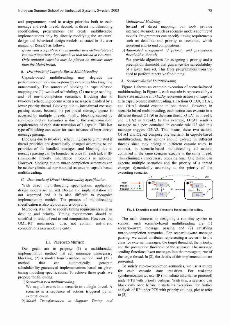
European Summer School on Embedded Systems, Sweden, 2003
78
and programmers need to assign priorities both to each message and each thread. Second, in direct multithreading specification, programmers can create multithreaded implementations only by directly modifying the structural design and behavioral design models, as stated in the user manual of RoseRT as follows.
If you want a capsule to run in another user-defined thread, you must incarnate that capsule in that thread at run-time. Only optional capsules may be placed on threads other than the MainThread.
B. Drawbacks of Capsule-Based Multithreading Capsule-based multithreading may degrade the
performance of real-time systems by extending blocking time unnecessarily. The sources of blocking in capsule-based mapping are (1) two-level scheduling, (2) message sending, and (3) run-to-completion semantics. Blocking due to two-level scheduling occurs when a message is handled by a lower priority thread. Blocking due to inter-thread message passing occurs because the per-thread message queue is accessed by multiple threads. Finally, blocking caused by run-to-completion semantics is due to the synchronization requirements of each state transition of a capsule. This last type of blocking can occur for each instance of inter-thread message passing.
Blocking due to two-level scheduling can be eliminated if thread priorities are dynamically changed according to the priorities of the handled messages, and blocking due to message passing can be bounded as once for each task if IIP (Immediate Priority Inheritance Protocol) is adopted. However, blocking due to run-to-completion semantics can be neither eliminated nor bounded as once in capsule-based multithreading.
C. Drawbacks of Direct Multithreading Specification With direct multi-threading specification, application
design models are blurred. Design and implementation are not separated and it is also difficult to recognize implementation models. The process of multithreading specification is also tedious and error-prone.
Moreover, it is hard to specify timing requirements such as deadline and priority. Timing requirements should be specified in units of end-to-end computation. However, the UML-RT meta-model does not contain end-to-end computations as a modeling entity
III. PROPOSED METHOD Our goals are to propose (1) a multithreaded
implementation method that can minimize unnecessary blocking, (2) a model transformation method, and (3) a method that can automatically generate schedulability-guaranteed implementations based on given timing modeling specifications. To achieve these goals, we propose the following:
1) Scenario-based multithreading: We map all events in a scenario to a single thread. A scenario is a sequence of actions triggered by an external event.
2) Model Transformation to Support Timing and
Multithread Modeling: Instead of direct mapping, our tools provide intermediate models such as scenario models and thread models. Programmers can specify timing requirements such as deadline and priority to scenarios, which represent end-to-end computations.
3) Automated assignment of priority and preemption threshold to threads: We provide algorithms for assigning a priority and a preemption threshold that guarantee the schedulability of a given task set. This frees programmers from the need to perform repetitive fine-tuning.
A. Scenario-Based Multithreading Figure 1 shows an example execution of scenario-based
multithreading. In Figure 1, each capsule is represented by a finite state machine and Ox:Ay represents action y of capsule x. In capsule-based multithreading, all actions O1:A0, O1:A1, and O1:A2 should execute in one thread. However, in scenario-based multithreading, each action can execute in a different thread: O1:A0 in the main thread, O1:A1 in thread1, and O1:A2 in thread2. In this example, O1:A1 sends a message to a port contained in capsule role O2 and this message triggers O2:A2. This means these two actions O1:A1 and O2:A2 compose one scenario. In capsule-based multithreading, these actions should execute in different threads since they belong to different capsule roles. In contrast, in scenario-based multithreading all actions contained in the same scenario execute in the same thread. This eliminates unnecessary blocking time. One thread can execute multiple scenarios and the priority of a thread changes dynamically according to the priority of the executing scenario.
send()S2
S1S1
S2
send()
O1 O2
mainthread1 thread2 A1 A1 A2A2
A0 A0
Fig. 1. Execution model of scenario-based multithreading.
The main concerns in designing a run-time system to support such scenario-based multithreading are (1) scenario-aware message passing and (2) satisfying run-to-completion semantics. For scenario-aware message passing, we added attributes representing a scenario to the class for external messages; the target thread id, the priority, and the preemption threshold of the scenario. The message sending functions insert messages into the message queue of the target thread. In [2], the details of this implementation are presented.
To satisfy run-to-completion semantics, we use a mutex for each capsule state transition. For real-time synchronization we use IIP (immediate inheritance protocol) under PTS with priority ceilings. With this, a scenario can block only once before it starts its execution. For further analysis of IIP under PTS with priority ceilings, please refer to [3].
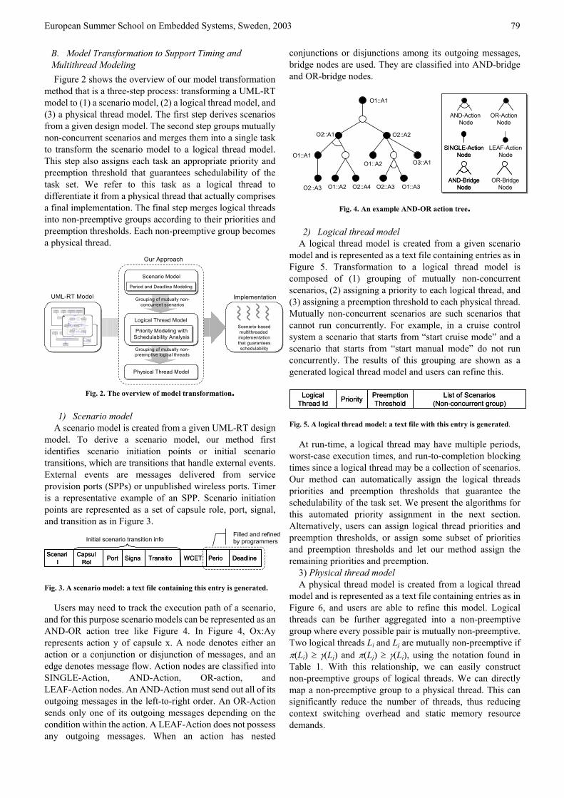
European Summer School on Embedded Systems, Sweden, 2003
79
B. Model Transformation to Support Timing and Multithread Modeling Figure 2 shows the overview of our model transformation
method that is a three-step process: transforming a UML-RT model to (1) a scenario model, (2) a logical thread model, and (3) a physical thread model. The first step derives scenarios from a given design model. The second step groups mutually non-concurrent scenarios and merges them into a single task to transform the scenario model to a logical thread model. This step also assigns each task an appropriate priority and preemption threshold that guarantees schedulability of the task set. We refer to this task as a logical thread to differentiate it from a physical thread that actually comprises a final implementation. The final step merges logical threads into non-preemptive groups according to their priorities and preemption thresholds. Each non-preemptive group becomes a physical thread.
UML-RT Model Implementation
Scenario-basedmultithreaded implementationthat guaranteesschedulability
Our Approach
Physical Thread ModelPhysical Thread Model
Grouping of mutually non-concurrent scenarios
Period and Deadline ModelingPeriod and Deadline Modeling
Scenario Model
Grouping of mutually non-preemptive logical threads
Logical Thread Model
Priority Modeling withSchedulability AnalysisPriority Modeling with
Schedulability Analysis
Fig. 2. The overview of model transformation.
1) Scenario model A scenario model is created from a given UML-RT design
model. To derive a scenario model, our method first identifies scenario initiation points or initial scenario transitions, which are transitions that handle external events. External events are messages delivered from service provision ports (SPPs) or unpublished wireless ports. Timer is a representative example of an SPP. Scenario initiation points are represented as a set of capsule role, port, signal, and transition as in Figure 3.
Fig. 3. A scenario model: a text file containing this entry is generated.
Users may need to track the execution path of a scenario, and for this purpose scenario models can be represented as an AND-OR action tree like Figure 4. In Figure 4, Ox:Ay represents action y of capsule x. A node denotes either an action or a conjunction or disjunction of messages, and an edge denotes message flow. Action nodes are classified into SINGLE-Action, AND-Action, OR-action, and LEAF-Action nodes. An AND-Action must send out all of its outgoing messages in the left-to-right order. An OR-Action sends only one of its outgoing messages depending on the condition within the action. A LEAF-Action does not possess any outgoing messages. When an action has nested
conjunctions or disjunctions among its outgoing messages, bridge nodes are used. They are classified into AND-bridge and OR-bridge nodes.
O2::A3 O1::A2 O2::A4 O2::A3 O1::A3
O3::A1O1::A2O1::A1
O2::A1 O2::A2
O1::A1
AND-Action Node
OR-ActionNode
OR-BridgeNode
AND-BridgeNode
AND-BridgeNode
SINGLE-ActionNode
SINGLE-ActionNode
LEAF-ActionNode
Fig. 4. An example AND-OR action tree.
2) Logical thread model A logical thread model is created from a given scenario
model and is represented as a text file containing entries as in Figure 5. Transformation to a logical thread model is composed of (1) grouping of mutually non-concurrent scenarios, (2) assigning a priority to each logical thread, and (3) assigning a preemption threshold to each physical thread. Mutually non-concurrent scenarios are such scenarios that cannot run concurrently. For example, in a cruise control system a scenario that starts from “start cruise mode” and a scenario that starts from “start manual mode” do not run concurrently. The results of this grouping are shown as a generated logical thread model and users can refine this.
List of Scenarios
(Non-concurrent group)Preemption ThresholdPriorityLogical
Thread IdList of Scenarios
(Non-concurrent group)Preemption ThresholdPriorityLogical
Thread Id Fig. 5. A logical thread model: a text file with this entry is generated.
At run-time, a logical thread may have multiple periods, worst-case execution times, and run-to-completion blocking times since a logical thread may be a collection of scenarios. Our method can automatically assign the logical threads priorities and preemption thresholds that guarantee the schedulability of the task set. We present the algorithms for this automated priority assignment in the next section. Alternatively, users can assign logical thread priorities and preemption thresholds, or assign some subset of priorities and preemption thresholds and let our method assign the remaining priorities and preemption.
Filled and refined Initial scenario transition info by programmers
ScenariScenari CapsulCapsul Port Port SignaSigna TransitioTransitio WCETWCET PerioPerio DeadlineDeadlineII RolRol
3) Physical thread model A physical thread model is created from a logical thread
model and is represented as a text file containing entries as in Figure 6, and users are able to refine this model. Logical threads can be further aggregated into a non-preemptive group where every possible pair is mutually non-preemptive. Two logical threads Li and Lj are mutually non-preemptive if π(Li) ≥ γ(Lj) and π(Lj) ≥ γ(Li), using the notation found in Table 1. With this relationship, we can easily construct non-preemptive groups of logical threads. We can directly map a non-preemptive group to a physical thread. This can significantly reduce the number of threads, thus reducing context switching overhead and static memory resource demands.

European Summer School on Embedded Systems, Sweden, 2003
80
List of Logical Threads (Mutually non-preemptive group)
PhysicalThread Id
List of Logical Threads (Mutually non-preemptive group)
PhysicalThread Id
Fig. 6. A physical thread model: a text file with this entry is generated.
C. Automated Priority and Preemption Threshold Assignment For feasible priority assignment, our method adopts
Audsley's algorithm. For schedulability testing, our method uses response time analysis. Considering that logical threads have multiple scheduling attributes, our method extended existing response time analysis as follows according to the notations of Table 1.
Table 1. Notations for describing response time analysis algorithms.
Notation Description Li A logical thread τi A scenario τj
i A scenario mapped to logical thread Lj Aj
i An action composing scenario τj O(Aj
i) A capsule that contains action Aji
C(τi) The worst-case execution time of scenario τi T(τi) The period of scenario τi β(τi) The blocking time of scenario τi
π(X) The fixed-priority of X that may be either scenario τi or logical thread Li
γ(X) The preemption threshold of X that may be either scenario τi or logical thread Li
B(Li) The blocking time of logical thread Li due to preemption threshold scheduling
S(Li) The start time of logical thread Li F(Li) The finish time of logical thread Li R(Li) The response time of logical thread Li
( )
==
≥<
)()(::)(maxmax,)()(:
),()(:
hm
lk
lk
mkhli AOAOAC
ihilτπτπ
τπτπτβ
∑>
∀
⋅
++=
)()(
)()()(
max
)()(max)(
iLjLj
jkj
k
i
k
ij
ijji
CT
LR
CLR
ππ
ττ
ττβ
The higher the preemption threshold a task has, the lower number of context switches the task will incur. Therefore, our method assigns each logical thread the maximum possible preemption threshold. Our algorithm for assigning maximum preemption thresholds exploits the method presented in [4]. The response time analysis algorithm for logical threads with assigned preemption thresholds is as follows.
)()()(::)(max)(, jij
jkkji LLLCLB ππγτ >≥=
∑
≥≠∀
⋅
+
+=
)()(,
)()()(
1max
)(max),(max)(
iLjLjij
jkj
k
i
k
ijjii
CT
LS
LBLS
ππ
ττ
τβ
∑>
∀
⋅
+−
++==
)()(
)()()(
1)()(
max
)(max)()()(
iLiLj
jkj
k
ij
k
i
k
ijjiii
CT
LST
LF
CLSLFLR
γπ
τττ
τ
IV. CONCLUSION We have proposed a method for schedulability-aware
scenario-based multithreading for UML-RT models. Using our method it is possible to easily define timing requirements for an end-to-end computation and automatically generate a schedulability-guaranteed implementation.
Our scenario-based multithreading outperforms capsule-based multithreading because scenario-based multithreading (1) eliminates the blocking due to message passing that cannot be avoided in capsule-based multithreading and (2) our preemption threshold scheduling bounds as once the blocking due to run-to-completion. Please refer to [2] for our experimental results.
While enhancing the performance of multithreaded models, our model transformation also eliminates the mix of implementation and design that is present in the current RoseRT tool. Our method also enables programmers to specify timing requirements such as deadline and priority without modifying original models.
Also, our method automatically generates implementations that guarantee schedulability. With this, programmers do not need to generate implementations repeatedly or perform tedious fine-tuning.
REFERENCES [1] Kim, S. Hong, and N. Chang. Scenario-based implementation
architecture for real-time object-oriented models. In Proceedings of IEEE International Workshop on Object-oriented Real-time Dependable Systems (WORDS), 2002.
[2] J. Masse, S. Kim, and S. Hong. Tool set implementation for scenario-based multithreading of UML-RT models and experimental validation. In IEEE Real-Time/Embedded Technology and Applications Symposium (RTAS), 2003.
[3] S. Kim, S. Hong, and T.-H. Kim. Perfecting preemption threshold scheduling for object-oriented real-time system design: from the perspective of real-time synchronization. In Proceedings of ACM SIGPLAN Conference on Languages, Compilers, and Tools for Embedded Systems (LCTES), 2002.
[4] M. Saksena and Y. Wang, "Scalable real-time system design using preemption thresholds," Proceedings of IEEE Real-Time Systems Symposium, pp. 25 -34, 2000.