Motion Control (wheeled robots) - University of Maryland,...
53
Autonomous Mobile Robots, Chapter 3 © R. Siegwart, I. Nou Motion Control (wheeled robots) • Requirements for Motion Control Kinematic / dynamic model of the robot Model of the interaction between the wheel and the ground Definition of required motion -> speed control, position control Control law that satisfies the requirements "Position" Global Map Perception Motion Control Cognition Real World Environment Localization Path Environment Model Local Map
Transcript of Motion Control (wheeled robots) - University of Maryland,...

Autonomous Mobile Robots, Chapter 3
© R. Siegwart, I. Nourbakhsh
Motion Control (wheeled robots)
• Requirements for Motion Control Kinematic / dynamic model of the robot Model of the interaction between the
wheel and the ground Definition of required motion ->
speed control, position control Control law that satisfies the requirements
3
"Position" Global Map
Perception Motion Control
Cognition
Real WorldEnvironment
Localization
PathEnvironment ModelLocal Map

Autonomous Mobile Robots, Chapter 3
© R. Siegwart, I. Nourbakhsh
Introduction: Mobile Robot Kinematics
• Aim Description of mechanical behavior of the robot for
design and control Similar to robot manipulator kinematics However, mobile robots can move unbound with respect to its
environmento there is no direct way to measure the robot’s positiono Position must be integrated over timeo Leads to inaccuracies of the position (motion) estimate
-> the number 1 challenge in mobile robotics
Understanding mobile robot motion starts with understanding wheelconstraints placed on the robots mobility
3

Autonomous Mobile Robots, Chapter 3
© R. Siegwart, I. Nourbakhsh
• Representing robot within an arbitrary initial frame Initial frame: Robot frame:
Robot position:
Mapping between the two frames
Representing Robot Position
[ ]TI yx θξ =
{ }IIYX ,
{ }RRYX ,
( )!!!
"
#
$$$
%
&
'=
100
0cossin
0sincos
((
((
(R
( ) ( ) [ ]TIR yxRR θθξθξ
.....==
YR
XR
YI
XI
!
P
YR
XR
!
YI
XI
3.2.1

Autonomous Mobile Robots, Chapter 3
© R. Siegwart, I. Nourbakhsh
Mapping Between Frames: Details
ξξRR = R( = R(θθ) ) ξξII = = yx
θ...
cos cosθθ sinsinθθ 00-sin -sin θθ coscosθθ 00 00 00 11
. .
θθ
AA
BB
What isWhat is |A||A|coscosθθ ? ?
P
YR
XR
!
YI
XI
xcosxcosθθ + + ysinysinθθ-xsin-xsinθθ + + ycosycosθθ θθ
==
. ...
.
RecallRecall•• coscos((ππ / 2 - / 2 - θθ) = sin() = sin(θθ))•• coscos((ππ / 2 + / 2 + θθ) = -sin() = -sin(θθ))

Autonomous Mobile Robots, Chapter 3
© R. Siegwart, I. Nourbakhsh
Example
3.2.1

Autonomous Mobile Robots, Chapter 3
© R. Siegwart, I. Nourbakhsh
Introduction: Kinematics Model• Goal:
establish the robot speed as a function of the wheel speeds ,steering angles , steering speeds and the geometric parameters of therobot (configuration coordinates).
[ ]T
yx θξ....
=
iβ. iϕ
. i
!
3.2.1
ϕϕ.. ββ
ϕϕ measured in radians/sec, so measured in radians/sec, so ϕϕ/2/2ππ is revolutions/sec is revolutions/secIn one revolution wheel translates 2In one revolution wheel translates 2ππr linear unitsr linear unitsTranslational velocity is Translational velocity is 22ππr(r(ϕϕ//22ππ) = r) = rϕϕ
..
.. ..
..

Autonomous Mobile Robots, Chapter 3
© R. Siegwart, I. Nourbakhsh
Introduction: Kinematics Model• Goal:
establish the robot speed as a function of the wheel speeds ,steering angles , steering speeds and the geometric parameters of therobot (configuration coordinates).
Forward kinematics - “If I do this, what will happen?”
Inverse kinematics - “If I want this to happen, what should I do?”
),,,,, ( 111 mmnfyx
ββββϕϕ
θ
ξ.….….….
.
.
..
=
[ ]T
yx θξ....
=
iβ. iϕ
. i
!
[ ] ),, ( 111 θββββϕϕ....….….…. yxf
Tmmn =
3.2.1
=

Autonomous Mobile Robots, Chapter 3
© R. Siegwart, I. Nourbakhsh
Forward Kinematic Models - Differential Drive
• The robot Two wheels - radius r Point P centered between wheels Each wheel is distance l from P Wheels have rotational velocity ϕ1 and ϕ2
• Forward kinematic model
• Use ξξRR = R( = R(θθ) ) ξξII so so ξξII = R = R-1-1((θθ) ) ξξRR
3.2.2
.. ..
ξξII = = yx
θ...
.== f(l, r, f(l, r, θ, , ϕ1, ϕ2))
.. .. rrll
pp..
........
XXRR
YYRR

Autonomous Mobile Robots, Chapter 3
© R. Siegwart, I. Nourbakhsh
Differential Drive (cont.)
• Use ξξRR = R( = R(θθ) ) ξξII so so ξξII = R = R-1-1((θθ) ) ξξRR• Compute how wheel speeds influence ξξRR• Translate to ξξII via RR-1-1((θθ))
• Contribution to translation along XR• If one wheel spins and the other remains still P will move at half the
translational velocity of the wheel: 1/2rϕ1 or 1/2rϕ2• Sum these components to account for both wheels spinning
XR = 1/2rϕ1 + 1/2rϕ2
• Suppose they spin in opposite directions, same direction
.. .. .. ....
..
.. ..
rrll
pp..
XXRR
YYRR
.. ....

Autonomous Mobile Robots, Chapter 3
© R. Siegwart, I. Nourbakhsh
Differential Drive (cont.)
• Wheel rotation never contributes to YR. Why?• What about θ?
Wheel 1 spin makes robot rotate counterclockwise Pivot around wheel 2 (left wheel) Translational velocity is rϕ Traces circle with radius 2l Rotational velocity 2π * rϕ / (2π * 2l) = rϕ / 2l Wheel 2 spin makes robot rotate clockwise Sum to get net effect: θ = (rϕ1 - rϕ2) / 2l
..
rrll
pp..
XXRR
YYRR..
..
.. ..
.. .. ..

Autonomous Mobile Robots, Chapter 3
© R. Siegwart, I. Nourbakhsh
Differential Drive: The Punch Line
ξξII = R = R-1-1((θθ) ) ξξRR = = RR-1-1((θθ))r(r(ϕϕ11 + + ϕϕ22)/ 2)/ 2
00r(r(ϕϕ11 - - ϕϕ22)/ 2l)/ 2l
.. .... ..
....

Autonomous Mobile Robots, Chapter 3
© R. Siegwart, I. Nourbakhsh
Wheel Kinematic Constraints: Assumptions
• Movement on a horizontal plane• Point contact of the wheels• Wheels not deformable• Pure rolling• No slipping, skidding or sliding• No friction for rotation around contact point• Steering axes orthogonal to the surface• Wheels connected by rigid frame (chassis)
rϕ.
v P
YR
XR
!
YI
XI
3.2.3

Autonomous Mobile Robots, Chapter 3
© R. Siegwart, I. Nourbakhsh
Wheel Kinematic Constraints:
Fixed Standard Wheel
3.2.3
Rolling constraint:Rolling constraint: all motion all motionalongalong wheel plane (in the directionwheel plane (in the directionof v) must be accompanied byof v) must be accompanied by thethesame amount of wheel spin so thatsame amount of wheel spin so thatthere is pure rolling at contact pointthere is pure rolling at contact point

Autonomous Mobile Robots, Chapter 3
© R. Siegwart, I. Nourbakhsh
Wheel Kinematic Constraints:
Fixed Standard Wheel
3.2.3
Sliding constraint:Sliding constraint: there can be there can beno motion orthogonal to wheelno motion orthogonal to wheelplane (perpendicular to v),plane (perpendicular to v),otherwise wheel skidsotherwise wheel skids

Autonomous Mobile Robots, Chapter 3
© R. Siegwart, I. Nourbakhsh
Wheel Kinematic Constraints:
Fixed Standard Wheel: Rolling Constraint
3.2.3

Autonomous Mobile Robots, Chapter 3
© R. Siegwart, I. Nourbakhsh
Wheel Kinematic Constraints:
Fixed Standard Wheel: Sliding Constraint
3.2.3

Autonomous Mobile Robots, Chapter 3
© R. Siegwart, I. Nourbakhsh
Example
• Suppose that the wheel A is in position such that•α = 0 and β = 0• This would place the contact point of the wheel on XI with the plane of
the wheel oriented parallel to YI. If θ = 0, then the sliding constraintreduces to:
3.2.3

Autonomous Mobile Robots, Chapter 3
© R. Siegwart, I. Nourbakhsh
Not Omnidirectional: Why?
3.2.3
Can constraints be satisfied for ANY Can constraints be satisfied for ANY ξξII??..
Autonomous Mobile Robots, Chapter 3
© R. Siegwart, I. Nourbakhsh
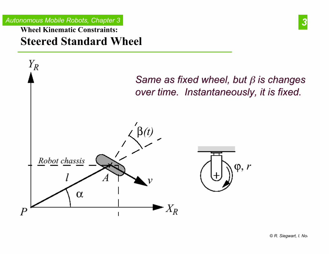
Wheel Kinematic Constraints:
Steered Standard Wheel
3.2.3
Same as fixed wheel, but Same as fixed wheel, but ββ is changes is changesover time. Instantaneously, it is fixed.over time. Instantaneously, it is fixed.

Autonomous Mobile Robots, Chapter 3
© R. Siegwart, I. Nourbakhsh
Wheel Kinematic Constraints:
Castor Wheel
3.2.3
•• Wheel contact point at BWheel contact point at B•• Steering at ASteering at A•• Rigid connector ABRigid connector AB

Autonomous Mobile Robots, Chapter 3
© R. Siegwart, I. Nourbakhsh
Wheel Kinematic Constraints:
Castor Wheel: Omnidirectional (why?)
3.2.3
[[coscos((αα + + ββ) sin() sin(αα + + ββ) ) d + d + lsinlsinββ]R(]R(θθ))ξξII + d + dββ = 0 = 0.. ..

Autonomous Mobile Robots, Chapter 3
© R. Siegwart, I. Nourbakhsh
Wheel Kinematic Constraints:
Swedish Wheel
3.2.3

Autonomous Mobile Robots, Chapter 3
© R. Siegwart, I. Nourbakhsh
Wheel Kinematic Constraints:
Spherical Wheel
3.2.3

Autonomous Mobile Robots, Chapter 3
© R. Siegwart, I. Nourbakhsh
Robot Kinematic Constraints
• Given a robot with M wheels each wheel imposes zero or more constraints on the robot motion only fixed and steerable standard wheels impose constraints
• What is the maneuverability of a robot considering a combination ofdifferent wheels?
• Suppose we have a total of N=Nf + Ns standard wheels We can develop the equations for the constraints in matrix forms: Rolling
Lateral movement( )1
)(
)()(
!+
"#
$%&
'=
sf NN
s
f
t
tt
(
((0)()( 21 =+ !"#$ && JRJ
Is
( ) 31
11
)()(
!+
"#
$%&
'=
sf NN
ss
fs
J
JJ
(( )( 12 NrrdiagJ L=
0)()(1 =Is RC !"# &
( ) 31
11
)()(
!+
"#
$%&
'=
sf NN
ss
fs
C
CC
((
3.2.4

Autonomous Mobile Robots, Chapter 3
© R. Siegwart, I. Nourbakhsh
Example: Differential Drive Robot
• Presented on blackboard
3.2.5

Autonomous Mobile Robots, Chapter 3
© R. Siegwart, I. Nourbakhsh
Example: Omnidirectional Robot
• Presented on blackboard
3.2.5

Autonomous Mobile Robots, Chapter 3
© R. Siegwart, I. Nourbakhsh
Mobile Robot Maneuverability
• The maneuverability of a mobile robot is the combination of the mobility available based on the sliding constraints plus additional freedom contributed by the steering
• Three wheels is sufficient for static stability additional wheels need to be synchronized this is also the case for some arrangements with three wheels
• It can be derived using the equation seen before Degree of mobility Degree of steerability Robots maneuverability
m!
s!
smM!!! +=
3.3

Autonomous Mobile Robots, Chapter 3
© R. Siegwart, I. Nourbakhsh
Mobile Robot Maneuverability: Degree of Mobility
• To avoid any lateral slip the motion vector has to satisfy thefollowing constraints:
• Mathematically: must belong to the null space of the projection matrix Null space of is the space N such that for any vector n in N
Geometrically this can be shown by the Instantaneous Center of Rotation(ICR)
0)(1 =If RC !" &
!"
#$%
&=
)()(
1
11
ss
fs
C
CC
''
0)()(1 =Iss RC !"# &
IR !" &)(
IR !" &)( )(1 sC !
)(1 sC !
0)(1 =!nC s"
3.3.1

Autonomous Mobile Robots, Chapter 3
© R. Siegwart, I. Nourbakhsh
Mobile Robot Maneuverability: Instantaneous Center of Rotation
• Ackermann Steering Bicycle
3.3.1

Autonomous Mobile Robots, Chapter 3
© R. Siegwart, I. Nourbakhsh
Mobile Robot Maneuverability: More on Degree of Mobility
• Robot chassis kinematics is a function of the set of independentconstraints the greater the rank of , the more constrained is the mobility
• Mathematically
o no standard wheelso all direction constrained
• Examples: Unicycle: One single fixed standard wheel Differential drive: Two fixed standard wheels
o wheels on same axleo wheels on different axle
[ ])(1 sCrank !
)(1 sC !
[ ] [ ])(3)(dim 11 ssm CrankCN !!" #== [ ] 3)(0 1 !! sCrank "
[ ] 0)(1 =sCrank !
[ ] 3)(1 =sCrank !
3.3.1

Autonomous Mobile Robots, Chapter 3
© R. Siegwart, I. Nourbakhsh
Mobile Robot Maneuverability: Degree of Steerability
• Indirect degree of motion
The particular orientation at any instant imposes a kinematic constraint However, the ability to change that orientation can lead additional
degree of maneuverability• Range of :
• Examples: one steered wheel: Tricycle two steered wheels: No fixed standard wheel car (Ackermann steering): Nf = 2, Ns=2 -> common axle
[ ])(1 sss Crank !" =
20 !!s
"s
!
3.3.2

Autonomous Mobile Robots, Chapter 3
© R. Siegwart, I. Nourbakhsh
Mobile Robot Maneuverability: Robot Maneuverability
• Degree of Maneuverability
Two robots with same are not necessary equal Example: Differential drive and Tricycle (next slide)
For any robot with the ICR is always constrainedto lie on a line
For any robot with the ICR is not constrained ancan be set to any point on the plane
• The Synchro Drive example:
smM!!! +=
M!
2=M
!
3=M
!
211 =+=+=smM
!!!
3.3.3

Autonomous Mobile Robots, Chapter 3
© R. Siegwart, I. Nourbakhsh
Mobile Robot Maneuverability: Wheel Configurations
• Differential Drive Tricycle
3.3.3

Autonomous Mobile Robots, Chapter 3
© R. Siegwart, I. Nourbakhsh
Five Basic Types of Three-Wheel Configurations
3.3.3

Autonomous Mobile Robots, Chapter 3
© R. Siegwart, I. Nourbakhsh
Synchro Drive
211 =+=+=smM
!!!
3.3.3

Autonomous Mobile Robots, Chapter 3
© R. Siegwart, I. Nourbakhsh
Mobile Robot Workspace: Degrees of Freedom
• Maneuverability is equivalent to the vehicle’s degree of freedom(DOF)
• But what is the degree of vehicle’s freedom in its environment? Car example
• Workspace how the vehicle is able to move between different configuration in its
workspace?• The robot’s independently achievable velocities
= differentiable degrees of freedom (DDOF) = Bicycle: DDOF = 1; DOF=3 Omni Drive: DDOF=3; DOF=3
m!
11+=+=smM
!!!
11+=+=smM
!!!
3.4.1

Autonomous Mobile Robots, Chapter 3
© R. Siegwart, I. Nourbakhsh
Mobile Robot Workspace: Degrees of Freedom, Holonomy
• DOF degrees of freedom: Robots ability to achieve various poses
• DDOF differentiable degrees of freedom: Robots ability to achieve various path
• Holonomic Robots A holonomic kinematic constraint can be expressed a an explicit function
of position variables only A non-holonomic constraint requires a different relationship, such as the
derivative of a position variable Fixed and steered standard wheels impose non-holonomic constraints
DOFDDOF m !! "
3.4.2

Autonomous Mobile Robots, Chapter 3
© R. Siegwart, I. Nourbakhsh
Mobile Robot Workspace:
Examples of Holonomic Robots
3.4.2

Autonomous Mobile Robots, Chapter 3
© R. Siegwart, I. Nourbakhsh
Path / Trajectory Considerations: Omnidirectional Drive
3.4.3

Autonomous Mobile Robots, Chapter 3
© R. Siegwart, I. Nourbakhsh
Path / Trajectory Considerations: Two-Steer
3.4.3

Autonomous Mobile Robots, Chapter 3
© R. Siegwart, I. Nourbakhsh
Beyond Basic Kinematics
3.5

Autonomous Mobile Robots, Chapter 3
© R. Siegwart, I. Nourbakhsh
Motion Control (kinematic control)
• The objective of a kinematic controller is to follow a trajectorydescribed by its position and/or velocity profiles as function of time.
• Motion control is not straight forward because mobile robots are non-holonomic systems.
• However, it has been studied by various research groups and someadequate solutions for (kinematic) motion control of a mobile robotsystem are available.
• Most controllers are not considering the dynamics of the system
3.6

Autonomous Mobile Robots, Chapter 3
© R. Siegwart, I. Nourbakhsh
Motion Control: Open Loop Control• trajectory (path) divided in motion segments of
clearly defined shape: straight lines and segments of a circle.
• control problem: pre-compute a smooth trajectory
based on line and circle segments• Disadvantages:
It is not at all an easy task to pre-computea feasible trajectory
limitations and constraints of the robotsvelocities and accelerations
does not adapt or correct the trajectory if dynamicalchanges of the environment occur.
The resulting trajectories are usually not smooth
yI
xI
goal
3.6.1

Autonomous Mobile Robots, Chapter 3
© R. Siegwart, I. Nourbakhsh
yR
xR
goal
v(t)
!(t)
"
starte
Motion Control: Feedback Control, Problem Statement
• Find a control matrix K, ifexists
with kij=k(t,e)• such that the control of v(t)
and ω(t)
• drives the error e to zero.
!"
#$%
&=
232221
131211
kkk
kkkK
!!!
"
#
$$$
%
&
'='=!"
#$%
&
()
y
x
KeKt
tv
R
)(
)(
0)(lim =!"te
t
3.6.2

Autonomous Mobile Robots, Chapter 3
© R. Siegwart, I. Nourbakhsh
Motion Control:
Kinematic Position Control
The kinematic of a differential drive mobilerobot described in the initial frame {xI, yI, θ} is given by,
where and are the linear velocities in thedirection of the xI and yI of the initial frame.Let α denote the angle between the xR axisof the robots reference frame and the vectorconnecting the center of the axle of thewheels with the final position.
!"
#$%
&
!!!
"
#
$$$
%
&
=
!!!
"
#
$$$
%
&
'(
(
(
vy
xI
10
0sin
0cos
&
&
&
3.6.2
Δy

Autonomous Mobile Robots, Chapter 3
© R. Siegwart, I. Nourbakhsh
Kinematic Position Control: Coordinates TransformationCoordinates transformation into polar coordinateswith its origin at goal position:
System description, in the new polar coordinates
3.6.2
Δy
for for

Autonomous Mobile Robots, Chapter 3
© R. Siegwart, I. Nourbakhsh
Kinematic Position Control: Remarks
• The coordinates transformation is not defined at x = y = 0; as in sucha point the determinant of the Jacobian matrix of the transformationis not defined, i.e. it is unbounded
• For the forward direction of the robot points towardthe goal, for it is the backward direction.
• By properly defining the forward direction of the robot at its initialconfiguration, it is always possible to have at t=0. Howeverthis does not mean that α remains in I1 for all time t.
3.6.2

Autonomous Mobile Robots, Chapter 3
© R. Siegwart, I. Nourbakhsh
Kinematic Position Control: The Control Law• It can be shown, that with
the feedback controlled system
• will drive the robot to• The control signal v has always constant sign,
the direction of movement is kept positive or negative during movement parking maneuver is performed always in the most natural way and
without ever inverting its motion.
( ) ( )000 ,,,, =!"#
3.6.2

Autonomous Mobile Robots, Chapter 3
© R. Siegwart, I. Nourbakhsh
Kinematic Position Control: Resulting Path
3.6.2

Autonomous Mobile Robots, Chapter 3
© R. Siegwart, I. Nourbakhsh
Kinematic Position Control: Stability Issue• It can further be shown, that the closed loop control system is locally
exponentially stable if
• Proof:for small x −> cosx = 1, sinx = x
and the characteristic polynomial of the matrix A of all roots
have negative real parts.
0 ; 0 ; 0 >!<> "#$" kkkk
3.6.2

Autonomous Mobile Robots, Chapter 3
© R. Siegwart, I. Nourbakhsh
Mobile Robot Kinematics: Non-Holonomic Systems
• Non-holonomic systems differential equations are not integrable to the final position. the measure of the traveled distance of each wheel is not sufficient to
calculate the final position of the robot. One has also to know how thismovement was executed as a function of time.
s1L s1R
s2L
s2R
yI
xI
x1, y1
x2, y2
s1
s2
s1=s2 ; s1R=s2R ; s1L=s2L
but: x1 = x2 ; y1 = y2
3.XX

Autonomous Mobile Robots, Chapter 3
© R. Siegwart, I. Nourbakhsh
Non-Holonomic Systems: Mathematical Interpretation• A mobile robot is running along a trajectory s(t).
At every instant of the movement its velocity v(t) is:
• Function v(t) is said to be integrable (holonomic) if there exists a trajectory function s(t)that can be described by the values x, y, and θ only.
• This is the case if
• With s = s(x,y,θ) we get for ds
yI
xI
s(t)
!
v(t)
!! sincos)(t
y
t
x
t
stv
"
"+
"
"=
"
"=
!! sincos dydxds +=
),,( !yxss =
y
s
y
s
x
s
x
s
xy
s
yx
s
!!
!=
!!
!
!!
!=
!!
!
!!
!=
!!
!
""""
222222
; ;
!!ds
dyy
sdxx
sds
"
"+
"
"+
"
"=
Condition for integrable function
3.XX

Autonomous Mobile Robots, Chapter 3
© R. Siegwart, I. Nourbakhsh
Non-Holonomic Systems: The Mobile Robot Example
• In the case of a mobile robot where
• and by comparing the equation above with
• we find
• Condition for an integrable (holonomic) function:
the second (-sinθ=0) and third (cosθ=0) term in equation do not hold!
!! sincos dydxds +=
!!ds
dyy
sdxx
sds
"
"+
"
"+
"
"=
0 ; sin ; cos =!
!=
!
!=
!
!
"""
s
y
s
x
s
y
s
y
s
x
s
x
s
xy
s
yx
s
!!
!=
!!
!
!!
!=
!!
!
!!
!=
!!
!
""""
222222
; ;
3.XX


