Lehrstuhl E15

Physik - Department

Monte Carlo Study of the FastNeutron Background in LENA

Diploma Thesis

Randolph Mollenberg30. November 2009

Technische UniversitatMunchen

Abstract

LENA (Low Energy Neutrino Astronomy) is a proposed next generationliquid-scintillator detector with about 50 kt target mass.Its main physics goals are the detection of solar neutrinos, supernova neu-trinos, geoneutrinos and the search for proton decay. Besides the directobservation of a supernova, LENA will also search for the so called diffusesupernova neutrino background (DSNB) that was generated by core-collapsesupernovae throughout the universe. Up to now the DSNB has not beendetected, due to the low flux. As only 6 to 13 DSNB events per year areexpected in LENA, background is a crucial issue for DSNB detection.Due to the delayed coincidence signal from the inverse beta decay detectionchannel, liquid-scintillator detectors offer a high background-discriminationefficiency. One remaining background source are fast neutrons that are pro-duced by muons in the surrounding rock and propagate into the detectorunnoticed, as these events mimic the same delayed coincidence signal. At-mospheric neutrinos generate also neutrons by neutral current reactions oncarbon in the scintillator.Therefore, a Monte Carlo simulation of neutron production in the rock and ofthe propagation into the detector was performed to determine the fast neu-tron background rates. Subsequently, possible methods for the identificationof fast neutron events were analyzed. As typical neutron interactions producepulse shapes different from positrons that are emitted in inverse beta decayreactions, neutron events can be identified by pulse shape analysis. Thus,an experiment was performed to investigate the efficiency of pulse shape dis-crimination in a small liquid-scintillator sample. The obtained results of thediscrimination efficiency and pulse shape parameters were used as input pa-rameters for the Monte Carlo Simulation of the LENA detector. Based onthis, the efficiency for neutron-νe discrimination was analyzed for the large-scale geometry of LENA. The neutron rejection efficiency was determinedto over 99.4% in PXE and over 99.0% in LAB, making a detection of theDSNB with a signal to background ratio of about 10:1 or better achievablewith both PXE and LAB in LENA.

II

Contents

1 Introduction 11.1 Neutrinos in the Standard Model . . . . . . . . . . . . . . . . 21.2 Neutrinos beyond the Standard Model . . . . . . . . . . . . . 3

1.2.1 Vacuum Neutrino Oscillations . . . . . . . . . . . . . . 31.2.2 The Mikheyev-Smirnov-Wolfenstein Effect . . . . . . . 4

1.3 Real-time Neutrino Detectors . . . . . . . . . . . . . . . . . . 61.3.1 Water-Cerenkov Detectors . . . . . . . . . . . . . . . . 71.3.2 Liquid-Scintillator Detectors . . . . . . . . . . . . . . . 10

2 The LENA Project 132.1 Detector Design . . . . . . . . . . . . . . . . . . . . . . . . . . 13

2.1.1 Detector Layout . . . . . . . . . . . . . . . . . . . . . . 132.1.2 Detector Location . . . . . . . . . . . . . . . . . . . . . 15

2.2 Physics Goals . . . . . . . . . . . . . . . . . . . . . . . . . . . 162.2.1 Solar Neutrinos . . . . . . . . . . . . . . . . . . . . . . 162.2.2 Supernova Neutrinos . . . . . . . . . . . . . . . . . . . 192.2.3 Diffuse Supernova Neutrino Background . . . . . . . . 202.2.4 Geoneutrinos . . . . . . . . . . . . . . . . . . . . . . . 222.2.5 Proton Decay . . . . . . . . . . . . . . . . . . . . . . . 252.2.6 Dark Matter Annihilation Neutrinos . . . . . . . . . . 25

3 Monte Carlo Simulations of the Fast Neutron Background inLENA 273.1 Neutron Production Processes . . . . . . . . . . . . . . . . . . 273.2 The GEANT4 Simulation Toolkit . . . . . . . . . . . . . . . . 293.3 Simulation Setup . . . . . . . . . . . . . . . . . . . . . . . . . 30

3.3.1 Detector Setup . . . . . . . . . . . . . . . . . . . . . . 303.3.2 Scintillation and Light Propagation . . . . . . . . . . . 31

3.4 Neutron Production . . . . . . . . . . . . . . . . . . . . . . . . 323.5 Neutron Propagation into the Detector . . . . . . . . . . . . . 383.6 Background Rates in LENA . . . . . . . . . . . . . . . . . . . 41

III

3.7 Identification of Neutron Events . . . . . . . . . . . . . . . . . 433.7.1 Multiple Neutron Capture Events . . . . . . . . . . . . 433.7.2 Pulse Shape Analysis . . . . . . . . . . . . . . . . . . . 44

4 Neutron-Gamma Pulse Shape Discrimination in Liquid Scin-tillators 474.1 Tail-to-total Discrimination Method . . . . . . . . . . . . . . . 474.2 Experimental Setup . . . . . . . . . . . . . . . . . . . . . . . . 484.3 Data Acquisition and Analysis . . . . . . . . . . . . . . . . . . 504.4 Results . . . . . . . . . . . . . . . . . . . . . . . . . . . . . . . 514.5 Monte Carlo Simulation . . . . . . . . . . . . . . . . . . . . . 54

5 Pulse Shape Discrimination of Neutron and νe Events inLENA 595.1 Simulation Setup . . . . . . . . . . . . . . . . . . . . . . . . . 595.2 Results . . . . . . . . . . . . . . . . . . . . . . . . . . . . . . . 61

6 Cosmogenic Background for the DSNB Detection 676.1 9Li In-situ Production . . . . . . . . . . . . . . . . . . . . . . 676.2 Muon-induced Neutrons . . . . . . . . . . . . . . . . . . . . . 686.3 Atmospheric Neutrinos . . . . . . . . . . . . . . . . . . . . . . 69

7 Conclusions and Outlook 73

List of Figures 78

List of Tables 79

Bibliography 81

IV

Chapter 1

Introduction

The neutrino was postulated in the 1930s by Wolfgang Pauli in order to con-serve energy, momentum, and spin for the β decay [1]. Neutrinos interactonly weakly, therefore they are not affected by electromagnetic fields andpoint directly back to their source, like photons do. But unlike electromag-netically interacting photons they are only marginally affected by matter.Therefore, neutrino astronomy provides a unique way to look inside manyastrophysical objects and phenomena, like core-collapse supernovae, the Sun,or the Earth itself [2].

The proposed LENA (Low Energy Neutrino Astronomy) detector is, due toits large target of ∼ 50 kt, capable of performing high-statistic measurementsof strong astrophysical neutrino sources as well as detecting rare neutrinoevents, like geoneutrinos (see Section 2.2.4) or diffuse supernova backgroundneutrinos (see Section 2.2.3). As only 6 to 13 DSNB events per year areexpected in LENA, background identification is crucial for its detection.One background source are fast neutrons, because they mimic the signatureof νe events. They are produced by cosmic muons in the surrounding rock ofthe detector and propagate into the detector unnoticed. Therefore, the fastneutron background rate in LENA as well as techniques for its suppressionwere analyzed in this thesis.

In the present Chapter a short introduction about neutrino physics in andbeyond the Standard Model of particle phyiscs will be given. Furthermore,a brief overview about Water-Cerenkov and liquid-scintillator neutrino de-tectors will be given. The experimental setup and the physics programm ofthe proposed LENA (Low Energy Neutrino Astronomy) detector will beoutlined in the second Chapter. In Chapter 3, the results of a Monte CarloSimulation of the fast neutron background in LENA will be presented. Theresults of a measurement of the pulse shape discrimination efficiency of neu-tron and gamma events in a small liquid-scintillator detector will be presented

1

Doublets Singlets(eLνe,L

)(µLνµ,L

)(τLντ,L

)eR µR τR

Table 1.1: Leptons in the scope of the weak interaction.

in Chapter 4. Subsequently, the efficiency of pulse shape discrimination ofneutron and νe events in LENA is determined by a Monte Carlo simulationin Chapter 5. Based on the resulting neutron rejection efficiency, the cos-mogenic background remaining for the DSNB detection will be analyzed inChapter 6.

1.1 Neutrinos in the Standard Model

In the Standard Model (SM) of particle physics, leptons and quarks aredivided into three generations [3]. Each generation consists of one chargedlepton (e, µ, τ), one corresponding neutrino (νe, νµ, ντ ) and 2 quarks. Forevery particle of the SM there exists one antiparticle, with the same mass andliftime but opposite quantum numbers. The left-handed eigenstates of thecharged leptons and their counterparting neutrino form doublets under theweak interaction, while the right-handed eigenstates of the charged leptonsare described as singlets (see Table 1.1) [4]. Neutrinos are generated only inleft-handed states and since the helicity is conserved (because neutrinos aremassless) they stay left-handed. Thus, right-handed neutrinos do not exist inthe standard model. Neutrinos only interact through the weak interaction.Parity is maximally violated in the weak interaction as the W± and Z0 vectorbosons couple only to left-handed particles and right-handed antiparticles [5].

The lepton flavour number is conserved in the Standard Modell, in the sensethat in every reaction the number of leptons from one generation must beconstant [3]. Therefore, charged current (CC) reactions can only occur withinone lepton doublet.

While the coupling constants of the weak interaction are comparable instrength to the coupling constant of the electromagnetic interaction, the factthat the exchange bosons are massive (mW± = 80 GeV, mZ0 = 91 GeV)severely reduces the strength and range of the weak interaction for low en-ergies [4].

Neutrinos with energies in the range of some MeV have consequently crosssections in the order of 10−43cm2 to 10−44cm2, resulting in a mean free pathλν ≈ 1018 m ≈ 100 light yrs in normal stellar matter with ρ ≈ 1 g

cm3 [3].

2

1.2 Neutrinos beyond the Standard Model

Contrary to the predictions of the SM, there are several evidences from solarneutrino experiments [6, 7], that there is a mixture between mass and flavoureigenstates as it is present in the quark sector, and that the neutrinos arenot massless.

1.2.1 Vacuum Neutrino Oscillations

The weak flavour eigenstates of the neutrino (νe, νµ, ντ ) can be expressed aslinear superpositions of orthogonal neutrino mass eigenstates (ν1, ν2, ν3) [8]: νe

νµντ

= U

ν1

ν2

ν3

(1.1)

U is the unitary Pontecorvo-Maki-Nakagawa-Sakata (PMNS) matrix. It canbe parameterized with three rotation angles θij and one CP violating phaseδ [9]:

U =

1 0 00 c23 s23

0 −s23 c23

c13 0 s13e−iδ

0 1 0−s13e

−iδ 0 c13

c12 s12 0−s12 c12 0

0 0 1

(1.2)

In this parameterization sij and cij are abbreviations of sin(θij) and cos(θij).The time evolution of the neutrino mass eigenstates is given by the Schrodingerequation1:

|νi(t)〉 = e−iEit|νi(0)〉 (1.3)

where Ei is the energy of the mass eigenstate νi.Assuming that the neutrino has a finite but small mass, such that mi � piand pi ≈ E, the neutrino energy Ei can be written as :

Ei =√p2i +m2

i ' pi +m2i

2pi' E +

m2i

2E(1.4)

From equations (1.1)-(1.4) it follows that the probability Pα→β to detecta neutrino in the flavour eigenstate β, which was produced in the flavoureigenstate α, is:

Pα→β = |〈νβ|vα(t)〉|2 , with |να〉 =∑i

Uαi|νi(t)〉 (1.5)

1In the following h = c = 1

3

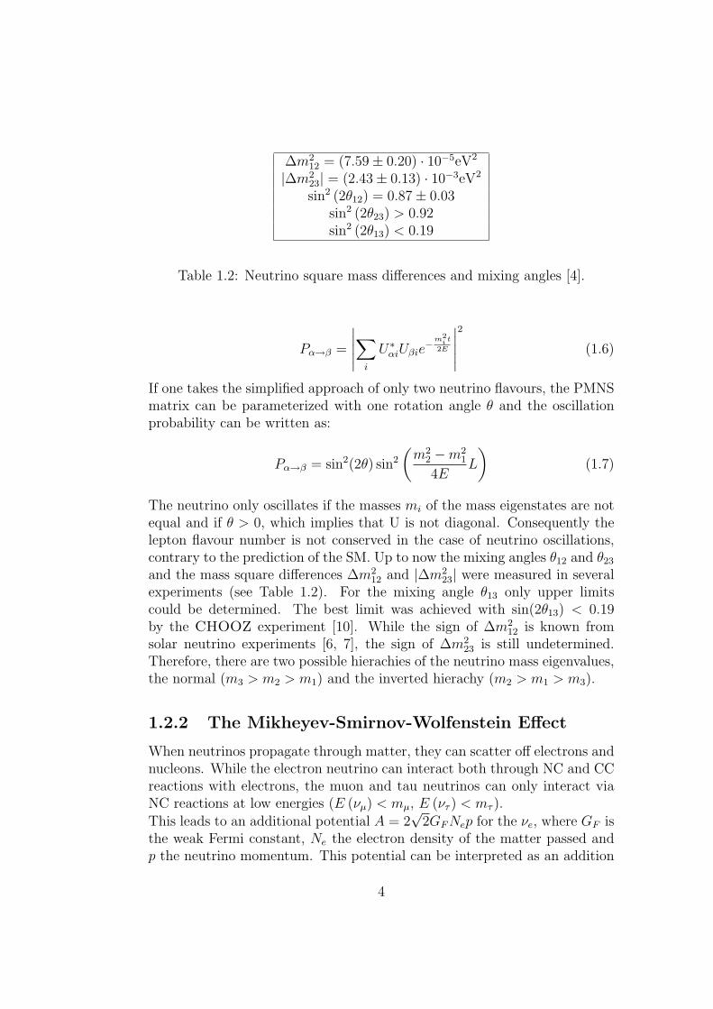
∆m212 = (7.59± 0.20) · 10−5eV2

|∆m223| = (2.43± 0.13) · 10−3eV2

sin2 (2θ12) = 0.87± 0.03sin2 (2θ23) > 0.92sin2 (2θ13) < 0.19

Table 1.2: Neutrino square mass differences and mixing angles [4].

Pα→β =

∣∣∣∣∣∑i

U∗αiUβie−m

2i t

2E

∣∣∣∣∣2

(1.6)

If one takes the simplified approach of only two neutrino flavours, the PMNSmatrix can be parameterized with one rotation angle θ and the oscillationprobability can be written as:

Pα→β = sin2(2θ) sin2

(m2

2 −m21

4EL

)(1.7)

The neutrino only oscillates if the masses mi of the mass eigenstates are notequal and if θ > 0, which implies that U is not diagonal. Consequently thelepton flavour number is not conserved in the case of neutrino oscillations,contrary to the prediction of the SM. Up to now the mixing angles θ12 and θ23

and the mass square differences ∆m212 and |∆m2

23| were measured in severalexperiments (see Table 1.2). For the mixing angle θ13 only upper limitscould be determined. The best limit was achieved with sin(2θ13) < 0.19by the CHOOZ experiment [10]. While the sign of ∆m2

12 is known fromsolar neutrino experiments [6, 7], the sign of ∆m2

23 is still undetermined.Therefore, there are two possible hierachies of the neutrino mass eigenvalues,the normal (m3 > m2 > m1) and the inverted hierachy (m2 > m1 > m3).

1.2.2 The Mikheyev-Smirnov-Wolfenstein Effect

When neutrinos propagate through matter, they can scatter off electrons andnucleons. While the electron neutrino can interact both through NC and CCreactions with electrons, the muon and tau neutrinos can only interact viaNC reactions at low energies (E (νµ) < mµ, E (ντ ) < mτ ).This leads to an additional potential A = 2

√2GFNep for the νe, where GF is

the weak Fermi constant, Ne the electron density of the matter passed andp the neutrino momentum. This potential can be interpreted as an addition

4

Figure 1.1: The MSW effect in the Sun [9]. Electron neutrinos are producedin the solar center at high electron densities in the matter eigenstate ν2,m.When the adiabatic condition (the density gradient being small in comparisonto the matter oscillation length) is fulfilled, the νe leaves the Sun in thevacuum eigenstate ν2, which has a great contribution to νµ.

to the mass terms in the Hamiltonian, that describes the propagation of theneutrino mass eigenstates.The vacuum mixing angle θ (in the following, the simplified approach of onlytwo neutrino flavours is taken again) is replaced by the matter mixing angleθm [9]

sin2(2θm) =sin2(2θ)(

cos(2θ)− A∆m2

)2+ sin2(2θ)

(1.8)

From equation (1.8) follows that at a critical density ρc, where cos(2θ) = A∆m2 ,

sin2(2θm) equals 1, independently of the vacuum mixing angle. For electronneutrinos that are produced in the center of the Sun, a resonant conversioninto νµ,τ occurs if they are generated at a higher electron density ne thanthe resonant density ne,res (see Figure 1.1), the so called Mikheev-Smirnov-Wolfenstein (MSW) effect [8]. As the resonant density ne,res depends on theneutrino energy, the MSW effect applies to the high-energetic neutrinos ofthe solar spectrum (see Figure 1.2).A νe that is generated in the center of the Sun, is produced only in the mattereigenstate ν2,m, because θm is close to 90◦, due to the high density. When theneutrino traverses the Sun, the density decreases until the critical density isreached.If the density gradient is small in comparison to the oscillation length, anadiabatic conversion occurs where the neutrio stays in the mass eigenstate

5

ν2,m. After the neutrino leaves the Sun, it remains in the mass eigenstate ν2

as it propagates to the earth.The probability to detect an electron neutrino is constant as no vacuumoscillations occur:

Pee = sin2(2θ12) ∼= 30% (1.9)

While the lower part of the solar neutrino spectrum, like the pp and 7Beneutrinos, is subject vacuum oscillations only, the high-energetic part of the8B spectrum is subject to the MSW effect (see Figure 1.2).

Figure 1.2: The survival probability of νe from the Sun. The survivalprobability according to the MSW effect (assuming a large mixing anglesin(2θ13) ≈ 0.2) is shown in black. Additionally, the measurements fromBorexino (7Be neutrinos), SNO (8B neutrinos), and the prediction for thepp solar neutrinos is shown.

1.3 Real-time Neutrino Detectors

The first detection of solar neutrinos was achieved in the Homestake experi-ment by Raymond Davis in the 1970s [11]. The detection reaction was

νe + 37Cl→ 37Ar + e− (1.10)

where the produced 37Ar nuclei had to be extracted from the 37Cl andcounted. With this technique, only a time- and energy-integrated measure-ment of the solar neutrino flux was possible. Furthermore, this experiment

6

was only sensitive to νe, while electron antineutrinos, muon, and tau neutri-nos could not be detected. After the Homestake experiment new neutrinodetectors were developed, which were able to measure the energy of a neutrinoin real-time. The first neutrino detectors of this type were Water-Cerenkovdetectors (WCDs), which are capable of measuring the direction of the incom-ing neutrino, but are only sensitive to the higher energetic solar neutrinos[7] (see Section 1.3.1). Later on, large-volume liquid-scintillator detectors(LSDs) also provided the possibility to perform real-time measurements ofthe neutrino flux. LSDs can not provide information on the direction of theneutrino, but have a much lower threshold than WCDs and can thus measurea large part of the solar spectrum [12] (see Section 1.3.2).

1.3.1 Water-Cerenkov Detectors

Figure 1.3: Cerenkov light emission of a particle moving faster than thespeed of light in a medium ( c

n). The interference of the spherical light waves

emitted along the particle track generates the characteristic conical shape ofthe light front [13].

If a charged particle moves faster than the speed of light in a medium ( cn),

it emits Cerenkov light. Due to the constructive interference of sphericallight waves emitted along the particle track, a conical front is generatedanalogously to a supersonic mach cone (see Figure 1.3) [13]. The opening

7

angle α of the cone depends on the velocity β = vc

of the charged particleand the refractive index n of the medium

cosα =1

βn(1.11)

From equation (1.11) follows that the maximum opening angle is given byαmax = arccos( 1

n). To generate Cerenkov light, the particle velocity must be

greater than cn. The threshold energy is therefore

Et = γmo =1√

1− n−2m0 (1.12)

For water n = 1.33 and thus Ew,t = 1.52m0 and αw,max = 41.4◦.The Cerenkov light yield in water is in the range of approximately 200 pho-tons per MeV [12]. These photons can be detected with photomultiplier tubes(PMTs). The direction of the light-emitting particle can be reconstructedfrom the orientation of the Cerenkov cone. Due to the low light yield, thedetection threshold is usually in the order of several MeV [14, 7].

KamiokaNDE/Super-Kamiokande

The KamiokaNDE detector [14] was the first experiment that could measuresolar neutrinos in real time. Originally constructed for the search for nucleondecay, it was also sensitive to neutrinos. It was shielded by 1000 m rock (2700m.w.e. depth) against cosmic muons. The target mass consisted of 2.1 kt purewater, monitored by 948 PMTs.The detection reaction was elastic scattering from neutrinos off electrons.After the neutrino scattered off the electron, the Cerenkov light of the elec-tron was detected. Due to the high threshold of 7.5 MeV, only 8B-neutrinoscould be detected [14]. The direction of the recoil electron is correlated withthe direction of the incident neutrino. This can be used for background sup-pression, as the recoil electron tracks of solar neutrinos always point awayfrom the Sun.KamiokaNDE was replaced in 1996 by Super-Kamiokande [7]. Super-Kamio-kande has a 22.5 kt fiducial mass of ultrapure water, observed by 11146PMTs. The threshold could be lowered to 5 MeV, but Super-Kamiokandeis still only sensitive to 8B-neutrinos (see Figure 2.4). After 1496 days ofdata taking, the measured flux for the 8B-neutrinos is [7]

Φ8B = (2.35± 0.02[stat.]± 0.08[syst.]) · 106cm−2s−1 (1.13)

This flux only accounts to approximately 47% of the flux predicted by theStandard Solar Model (SSM) [7]. As Super-Kamiokande is (due to the higher

8

cross section of CC reactions) predominantely sensitive to electron neutrinos,the difference between the predicted and the measured flux can be explainedby neutrino oscillations (see Section 1.2).

SNO

The solar neutrino experiment SNO (Sudbury Neutrino Observatory) used1 kt heavy water (D2O) as a target [6]. The detector is covered by 2 km rock,corresponding to 6 km w.e. shielding against cosmic muons. SNO uses threedetection reactions:

• Elastic scattering off electrons (ES)

ν + e− → ν + e− (1.14)

Electron neutrinos can interact via charged current (CC) and neutralcurrent (NC) reactions, muon and tau neutrinos only via NC reactions.The cross-section for νe is therefore about a factor of 6.6 higher thanfor νµ,τ .

• Deuteron dissociation

CC : νe +D → e− + 2p (1.15)

NC : ν +D → ν + n+ p (1.16)

The charged current reaction (1.15) is only sensitive to electron neutri-nos and gives the opportunity to measure the νe-flux alone. The neutralcurrent reaction 1.16 is sensitive to all neutrino flavours, and contraryto reaction 1.14 every flavour has the same cross section. Hence, it isa measure for the total neutrino flux.

The threshold of SNO was 5.5 MeV and the measured fluxes were [6]:

ΦCC = 1.72+0.05−0.05(stat.)+0.11

−0.11(syst.) · 106cm−2s−1 (1.17)

ΦES = 2.34+0.23−0.23(stat.)+0.15

−0.14(syst.) · 106cm−2s−1 (1.18)

ΦNC = 4.81+0.19−0.19(stat.)+0.28

−0.27(syst.) · 106cm−2s−1 (1.19)

The result for ΦNC is in good agreement with the predictions from the Stan-dard Solar Model [6]. The survival probability for electron neutrinos ΦCC

ΦNCis

determined to approximately 36%, which is due to the MSW effect in theSun. As muon and tau neutrinos also contribute to ΦES, the flux is greaterthan ΦCC , but lower than ΦNC , due to the reduced cross-sections for muonand tau neutrinos of reaction (1.14).

9

1.3.2 Liquid-Scintillator Detectors

A liquid scintillator consists of at least two components. An organic solventthat serves as target material and a solute at low concentration, the so-calledwavelength shifter. Both consist of aromatic molecules. When a chargedparticle moves through the solvent, the weakly bound electrons in the π-orbitals of the benzene rings get excited or ionized. A solvent moleculein an excited state can subsequently transfer its energy non-radiatively toanother solvent or solute molecule. Finally, a photon is emitted through de-excitation of a solute molecule. This photon has a larger wavelength thana photon directly emitted by the solvent. As organic solvents become moretransparent at longer wavelength, the shifted light can travel further distancesthrough the detector. Like in a WCD the light is detected by PMTs, thatcover the walls of the detector. Another advantage of the wavelength shifteris that the wavelength of the emitted photons can be adjusted to the regionwhere common PMTs are most efficient [12].The photons are emitted isotropically and within a few nanoseconds [15].Hence, using the photon arrival time and the hit pattern of the PMTs, theposition of the event vertex inside the detector volume can be reconstructed,but the directional information is usually lost.The light yield of a scintillator depends on the incident particle. Heavierparticles like protons and α-particles have a greater energy loss per unitpath length than lighter particles like electrons and muons. As a result, afteran event involving a heavy particle, the density of molecules in an excitatedstate along the particle track is larger than in the case of light particle. Thus,the reaction

S∗ + S∗ → S+ + S0 + e− (1.20)

is more likely to happen, where S∗ denotes an excitated molecule, S+ anionized molecule and S0 is a molecule in ground state. Therefore less energyis converted into light, as the ionized molecule does not generate scintilla-tion light [15]. The ratio of deposited to visible energy is described by thequenching factor. For α particles, quenching factors of more than 10 relativeto electron events can be reached in common scintillators [16].The great advantage of liquid-scintillator detectors (LSD) is that the lightyield is with ∼ 104 scintillation photons per MeV [15] much greater thanthe light yield of WCDs (200 photons per MeV). Thus, the energy resolutionis better and the detection threshold is much lower. In contrast to that,the isotropic emission of the scintillation light allows no reconstruction ofthe particle direction at low energies. Information on the incident particle’sdirection can only be gained for high-energetic events like cosmic muons oratmospheric neutrinos [17].

10

Depending on the neutrino flavour, there are several possible detection re-actions in a liquid-scintillator detector. The most important ones are elasticscattering off electrons (see reaction (1.14)) and the inverse beta decay chan-nel for νe:

νe + p→ n+ e+, n+ p→ d+ γ (2.2 MeV) (1.21)

The elastic scattering reaction has in principle no threshold. The actualthreshold of the detector is governed by intrinsic radioactive contaminants.As 14C is naturally abundant in organic scintillators, a neutrino detection atenergies below the end point of the 14C β-spectrum of 156 keV is not possible.The inverse beta decay reaction has a threshold of 1.8 MeV. It provides adelayed coincidence signal as the positron gives a prompt signal and theneutron is captured after ∼ 200µs on a free proton [18]. A WCD is alsosensitive to this reaction, but the 2.2 MeV γ from the neutron capture isbelow the detection threshold. Therefore, the background suppression for νedetection is much better in a LSD.

Borexino

Figure 1.4: The Borexino detector [19]. It consist of 270 t liquid scintillatorin the Inner Vessel, that is shielded by several layers of buffer liquid and water.The scintillation light is detected by 2212 PMTs.

Borexino is a solar neutrino experiment that is also sensitive to geo-νe andreactor-νe. It uses 280 t of liquid scintillator as a target. The scintillator

11

mixture consist of pseudocumene (PC, 1,2,4-trimethylbenzene), used as thesolvent, and 1.5g

lPPO (2,5-diphenyloxazole) as wavelength shifter. The scin-

tillator is contained in a transparent nylon membrane with a radius of 4.25 mand a thickness of 125µm, the so-called Inner Vessel (IV) (see Figure 1.4).The Inner Vessel is surrounded by a buffer liquid, contained in the OuterVessel (OV), with a radius of 5.5 m. It shields the Inner Vessel from externalradioactivity. The buffer liquid is composed of PC and 3 g

lDMP (dimethyl-

phytalate). It has nearly the same density as the scintillator in the IV,therefore buoyancy forces on the IV are reduced. The DMP quenches thescintillation yield of PC by a factor of ∼ 20. Therefore, almost no scintillationis generated in the buffer.The OV serves as a barrier to Radon diffusion and is placed in a StainlessSteel Sphere (SSS), with a radius of 6.85 m. The space between the OV andthe SSS is also filled with buffer liquid. 2212 PMTs are mounted to the SSS,corresponding to an optical coverage of 30% of the surface.The SSS is placed in a steel dome of 18 m diameter, 16.9 m height, which isfilled with 2.1 kt of deionized water. The outside of the SSS and the floorof the Outer Detector (OD) are equipped with 208 PMTs in total. The ODserves as an active muon veto. Muons traversing the OD produce Cerenkovlight, which is detected by the PMTs.Borexino is taking data since 2007 [20]. Due to the low radioactive back-ground level achieved, it could perform the first real time detection of 7Beneutrinos. Borexino measured an event rate of [21]

49± 3(stat.)± 4(syst.)counts

day · 100t(1.22)

corresponding to a flux of

Φ7Be = (5.08± 0.25) · 109cm−2s−1 (1.23)

The results are in good agreement with the predictions from the SSM takingneutrino oscillations into account.

12

Chapter 2

The LENA Project

LENA (Low Energy Neutrino Astronomy) has been proposed as a nextgeneration large volume liquid-scintillator detector [2]. Its target mass iswith ∼50 kt considerably larger than the target mass of the present liquid-scintillator detectors (Borexino: 300 t, KamLAND: 1000 t). This allowson the one hand high-statistic measurements of strong astrophysical neutrinosources like the Sun, and on the other hand the detection of rare events, suchas geoneutrinos (see Section 2.2.4) or diffuse supernova background neutrinos(see Section 2.2.3).

The LENA Project is currently in a design phase as a part of the LAGUNA(Large Apparatus for Grand Unification and Neutrino Astrophysics) col-laboration, that shall last until the end of 2010 [12] at least.

2.1 Detector Design

2.1.1 Detector Layout

Figure 2.1 shows a schematic overview of the current LENA design, accord-ing to a pre-design study for the Pyhasalmi location [22].

The detector consists of a 100 m high vertical steel cylinder with 30 m indiameter that is placed in a 115 m high cavern. A vertical design is favorablefor the construction of the steel cylinder. The cavern is elliptically shapedwith 50 m maximum diameter in order to minimize rock mechanical risk [22].

The steel tank is filled with liquid scintillator. Inside the steel cylinder, thevolume is divided by a thin Nylon Vessel into the buffer volume shieldingexternal radioactivity and the target volume of 13 m diameter and 100 mheight, corresponding to 5.3 · 104m3. At the moment the composition of theliquid scintillator is not decided, PXE (phenyl-xylyl-ethane) and LAB (lin-

13

Figure 2.1: Schematical view of the LENA detector [22]. The target vol-ume consists of 50 kt of liquid scintillator. It is surrounded by 2 m of non-scintillating buffer liquid. 13500 PMTs detecting the scintillation light areplaced on the inner surface of the steel cylinder, which contains the targetand buffer volume. The surrounding 2 m of water also serve as passive shield-ing and as an active Water-Cerenkov muon veto. Plastic scintillators on topof the detector complete the active muon veto.

14

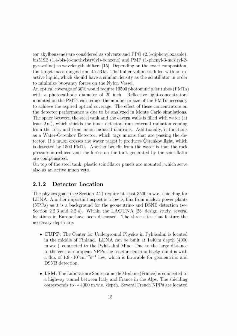
ear akylbenzene) are considered as solvents and PPO (2,5-diphenyloxazole),bisMSB (1,4-bis-(o-methylstrylyl)-benzene) and PMP (1-phenyl-3-mesityl-2-pyrazoline) as wavelength shifters [15]. Depending on the exact composition,the target mass ranges from 45-53 kt. The buffer volume is filled with an in-active liquid, which should have a similar density as the scintillator in orderto minimize buoyancy forces on the Nylon Vessel.An optical coverage of 30% would require 13500 photomultiplier tubes (PMTs)with a photocathode diameter of 20 inch. Reflective light-concentratorsmounted on the PMTs can reduce the number or size of the PMTs necessaryto achieve the aspired optical coverage. The effect of these concentrators onthe detector performance is due to be analyzed in Monte Carlo simulations.The space between the steel tank and the cavern walls is filled with water (atleast 2 m), which shields the inner detector from external radiation comingfrom the rock and from muon-induced neutrons. Additionally, it functionsas a Water-Cerenkov Detector, which tags muons that are passing the de-tector. If a muon crosses the water target it produces Cerenkov light, whichis detected by 1500 PMTs. Another benefit from the water is that the rockpressure is reduced and the forces on the tank generated by the scintillatorare compensated.On top of the steel tank, plastic scintillator panels are mounted, which servealso as an active muon veto.

2.1.2 Detector Location

The physics goals (see Section 2.2) require at least 3500 m.w.e. shielding forLENA. Another important aspect is a low νe flux from nuclear power plants(NPPs) as it is a background for the geoneutrino and DSNB detection (seeSection 2.2.3 and 2.2.4). Within the LAGUNA [23] design study, severallocations in Europe have been discussed. The three sites that feature thenecessary depth are:

• CUPP: The Center for Underground Physics in Pyhasalmi is locatedin the middle of Finland. LENA can be built at 1440 m depth (4000m.w.e.) connected to the Pyhasalmi Mine. Due to the large distanceto the central european NPPs the reactor neutrino background is witha flux of 1.9 · 105cm−2s−1 low, which is favorable for geoneutrino andDSNB detection.

• LSM: The Laboratoire Souterraine de Modane (France) is connected toa highway tunnel between Italy and France in the Alps. The shieldingcorresponds to ∼ 4000 m.w.e. depth. Several French NPPs are located

15

within 100 km distance, the reactor neutrino background is with a fluxof 1.6 · 106cm−2s−1 approximately one order of magnitude larger thanat the CUPP.

• Sunlab: The Sieroszowice Underground Laboratory (Poland) is lo-cated near Wroc law. The original plan was to use inactive shafts ofa salt mine in 950 m depth, but recently an investigation of a deeperlocation below the salt body has begun. A possible location for LENAat a depth corresponding to 3600 m.w.e. shielding has been found. Dueto the small thickness of the rock layer there, only a horizontal versionof LENA is possible at this site.

2.2 Physics Goals

2.2.1 Solar Neutrinos

In the Sun, energy is produced by nuclear fusion of hydrogen to helium intwo different reaction sequences, the pp-chain (Figure 2.2) and the CNO-cycle(Figure 2.3). In the pp-chain, helium is produced directly through the fusionof hydrogen, while in the CNO cycle 12C serves as a catalyst. The CNO-cycleis further divided into four sub-cycles, with the CNO-I cycle being the mostimportant of the four for the energy production in the Sun.While the pp-chain is dominating in the Sun and contributes to 98% ofits energy production, the CNO-cycle becomes dominant in larger stars ofmultiple solar masses. Both reaction mechanisms release 26.73 MeV energyin total and result in the same net reaction

4p→ 4He + 2e+ + 2νe (2.1)

Neutrinos from different reactions have different energies. The calculatedneutrino spectrum of the Sun according to the Standard Solar Model (SSM)[26] is shown in Figure 2.4.The detection threshold in LENA will be only limited by the radioactivecontamination. If the same level of radiopurity as present in Borexino wasachieved, a detection threshold of 250 keV should be possible.Table 2.1 shows the expected event rates for the elastic ν−e scattering chan-nel, using two different solar model predictions and assuming a conversativefiducial volume of 18 kt [12].Approximately 25 pp-ν events per day are expected above 250 keV. Thisrate is probably not high enough to distinguish the neutrino events from thenatural 14C background. With ∼ 5000 events per day, the 7Be − ν flux can

16

Figure 2.2: The single reactions of the pp-chain [24]. There are 4 reactionsthat generate neutrinos. The neutrinos from the pp and hep reaction havea continious energy spectrum, while the neutrinos from the 7Be and pepreaction are monoenergetic due to the kinematics of the reaction.

Figure 2.3: The CNO-I-cycle and CNO-II-cycle[25]. There are three reactionsgenerating neutrinos with a continious energy spectrum: 13N (CNO-I),15O(CNO-I and CNO-II) and 17F (CNO-II)

17

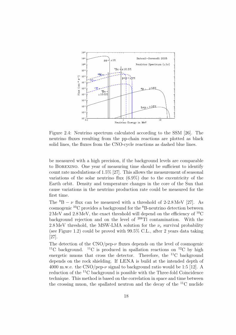
Figure 2.4: Neutrino spectrum calculated according to the SSM [26]. Theneutrino fluxes resulting from the pp-chain reactions are plotted as blacksolid lines, the fluxes from the CNO-cycle reactions as dashed blue lines.

be measured with a high precision, if the background levels are comparableto Borexino. One year of measuring time should be sufficient to identifycount rate modulations of 1.5% [27]. This allows the measurement of seasonalvariations of the solar neutrino flux (6.9%) due to the excentricity of theEarth orbit. Density and temperature changes in the core of the Sun thatcause variations in the neutrino production rate could be measured for thefirst time.

The 8B − ν flux can be measured with a threshold of 2-2.8 MeV [27]. Ascosmogenic 10C provides a background for the 8B-neutrino detection between2 MeV and 2.8 MeV, the exact threshold will depend on the efficiency of 10Cbackground rejection and on the level of 208Tl contamination. With the2.8 MeV threshold, the MSW-LMA solution for the νe survival probability(see Figure 1.2) could be proved with 99.5% C.L., after 2 years data taking[27].

The detection of the CNO/pep-ν fluxes depends on the level of cosmogenic11C background. 11C is produced in spallation reactions on 12C by highenergetic muons that cross the detector. Therefore, the 11C backgrounddepends on the rock shielding. If LENA is build at the intended depth of4000 m.w.e. the CNO/pep-ν signal to background ratio would be 1:5 [12]. Areduction of the 11C background is possible with the Three-fold Coincidencetechnique. This method is based on the correlation in space and time betweenthe crossing muon, the spallated neutron and the decay of the 11C nuclide

18

Source Event Rate [d−1]BPS08(GS) BPS08(AGS)

pp 24.92± 0.15 25.21± 0.13pep 365± 4 375± 4hep 0.16± 0.02 0.17± 0.037Be 4894± 297 4460± 2688B 82± 9 65± 7

CNO 545± 87 350± 52

Table 2.1: Solar neutrino event rates in LENA, assuming 18 kt fiducialvolume and 250 keV detection threshold, for high (BPS08(GS)) and low(BPS08(AGS)) solar metallicity [12].

[28]. At the moment the theoretical uncertainty of the CNO flux is with30% quite large. A high statistic measurement of this flux could provideinformation on the solar metallicity and test the accuracy of the currentsolar models.A measurement of the pep-ν flux could be used for a test of the νe survivalprobability in the energy region between 1 and 2 MeV, where the transitionbetween matter-induced to vacuum oscillations is predicted by the MSW-LMA solution. It also gives informations about the pp-flux, because the ratefor the pep reaction is proportional to that for the pp reaction [25].

2.2.2 Supernova Neutrinos

Stars with masses greater than 8 solar masses ( M�) build up a shell structurewith an iron core in the centre towards the end of their lifes [30]. Withincreasing density of the iron core, the gravitational pressure becomes higherthan the Fermi-pressure of the electrons and the core collapses until it reachesnuclear density, where the collapse is stopped by the Fermi pressure of theneutrons that are formed by the reaction (2.2). Further collapsing materialnow bounces on the ultra-dense core and builds an outward running shockfront.A supernova explosion releases ∼ 99% of its energy through neutrinos. Inthe first 20 ms of the supernova explosion νe are created by the reaction

e− + p→ n+ νe (2.2)

the so-called neutronisation burst. After that the core cools down throughemission of νν pairs of all flavours [30].

19

Detection Channel Event Rate(1) νe + p→ n+ e+ 7500-13800(2) νe +12 C→12 B + e+ 150-610(3) νe +12 C→12 N + e− 200-690(4) νe +13 C→13 N + e− ∼ 10(5) ν +12 C→12 C∗ + ν 680-2070(6) ν + e− → e− + ν 680(7) ν + p→ p+ ν 1500-5700(8) ν +13 C→13 C∗ + ν ∼ 10total 10000− 20000

Table 2.2: Expected event rates for a supernova explosion of a 8 M� star inthe center of our galaxy (d=8 kpc). The uncertainty in the event rates comesfrom different supernova explosion models and neutrino oscillation scenarios[29].

About one to three supernova explosions are expected in our galaxy percentury. If a 8 M� star explodes in the center of our galaxy (10 kPc distance),10000-20000 neutrino events are expected in LENA. Table 2.2 shows thepredicted event rates of a supernova explosion in the center of our galaxy inLENA, for the different detection channels. While the first four channels arecharged current (CC) reactions and allow a separate measurement of νe and νeevents, the last 4 channels are neutral current (NC) reactions and measure thesum of all flavours. The NC-channels are therefore not affected by neutrinooscillations and depend only on the supernova model. With the inverse betadecay channel (1) the νe spectrum and the temporal evolution of the νe-fluxcan be studied. The transit of νe’s through the matter of the progenitor starenvelope or of the Earth leaves an imprint on the νe spectrum. The survivalprobability of the electron and antielectron neutrinos depends on the neutrinomass hierarchy and, amongst others, on the unknown mixing angle θ13 [29].Thus, a measurement of the νe and νe spectrum gives information about themixing angle θ13 and the neutrino mass hierarchy.About 74 νe-events from the neutronisation burst are expected in LENA [29].A measurement of the neutronisation burst would give valuable informationabout the details of the core-collapse process.

2.2.3 Diffuse Supernova Neutrino Background

Core-collapse supernovae explosions throughout the universe have generateda cosmic neutrino background, the so called diffuse supernova neutrino back-

20

ground (DSNB). It contains information about the core-collapse supernovaexplosion mechanism itself, about the supernova rate (SNR) and about thestar formation rate up to high redshifts of z ' 5 [18]. The predicted fluxis with ∼ 102 cm−2s−1 about 8 orders of magnitudes smaller than the solarneutrino flux [18]. Up to now the DSNB could not be detected. The Super-Kamiokande experiment provides the best limit of 1.2 νe cm−2s−1 for energiesabove 19.3 MeV [31].

As all neutrino and antineutrino flavours are produced in a supernova explo-sion, the inverse beta decay channel, which has a low threshold (1.8 MeV)and the largest cross section at low energies, can be used for the detection ofthe DSNB:

νe + p→ n+ e+ (2.3)

The neutron is much heavier than the positron, therefore the positron getsalmost all the energy of the νe, but reduced by ∼ 1.8 MeV, due to the Q-Valueof reaction (2.3). However, the annihilation of the positron adds 2 mec

2 tothe signal, thus leading to a total reduction of 0.8 MeV. While the positrongives a prompt signal, the neutron is captured by free protons after ∼ 200µs:

n+ p→ d+ γ (2.2 MeV) (2.4)

The 2.2 MeV γ gives a delayed coincidence signal, therefore DSNB eventscan be seperated from radioactive background events. While the thresholdof Water-Cerenkov detectors lies above 2.2 MeV, liquid scintillator detectorslike LENA can easily detect the delayed coincidence signal from the neutroncapture on a free proton.

Reactor and atmospheric νe give an indistinguishable background to theDSNB signal. The background from reactor νe sets a lower limit for theDSNB search at E(νe) ∼ 10 MeV, the exact limit depends on the detectorsite. Figure 2.5 shows the reactor νe spectrum at various sites compared tothe expected DSNB spectrum.

Atmospheric νe exceed the DSNB signal at about 25 MeV, thus definingan upper limit. Therefore, a window between approximately 10 MeV and25 MeV is left for the DSNB detection (see Figure 2.6). Exact values dependon the detector site.

In this energy region 6 to 13 events will be detected in LENA per year. In-situ produced 9Li, muon-induced fast neutrons and neutral current reactionsfrom atmospheric neutrinos provide an additional background. A detailedanalysis of this background and the consequences for the DSNB detectionwill be given in Chapter 6.

21

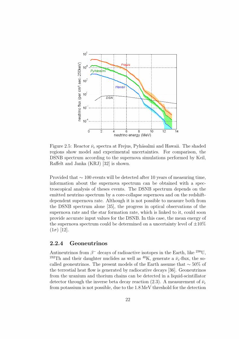
Figure 2.5: Reactor νe spectra at Frejus, Pyhasalmi and Hawaii. The shadedregions show model and experimental uncertainties. For comparison, theDSNB spectrum according to the supernova simulations performed by Keil,Raffelt and Janka (KRJ) [32] is shown.

Provided that ∼ 100 events will be detected after 10 years of measuring time,information about the supernova spectrum can be obtained with a spec-troscopical analysis of theses events. The DSNB spectrum depends on theemitted neutrino spectrum by a core-collapse supernova and on the redshift-dependent supernova rate. Although it is not possible to measure both fromthe DSNB spectrum alone [35], the progress in optical observations of thesupernova rate and the star formation rate, which is linked to it, could soonprovide accurate input values for the DSNB. In this case, the mean energy ofthe supernova spectrum could be determined on a uncertainty level of ±10%(1σ) [12].

2.2.4 Geoneutrinos

Antineutrinos from β− decays of radioactive isotopes in the Earth, like 238U,232Th and their daughter nuclides as well as 40K, generate a νe-flux, the so-called geoneutrinos. The present models of the Earth assume that ∼ 50% ofthe terrestial heat flow is generated by radiocative decays [36]. Geoneutrinosfrom the uranium and thorium chains can be detected in a liquid-scintillatordetector through the inverse beta decay reaction (2.3). A measurement of νefrom potassium is not possible, due to the 1.8 MeV threshold for the detection

22

Figure 2.6: Expected event rates of DSNB νe for LENA in Pyhasalmi ac-cording to the supernova simulations performed by the Lawrence LivermoreGroup (LL) [33], by Keil, Raffelt, and Janka (KRJ) [32], and by Thompson,Burrows, and Pinto (TBP) [34]. The reactor νe , atmospheric νe, and theSuper-Kamiokande limit are also shown. The shaded region represents thepossible DSNB νe event range due to uncertainties of the Supernova rate.

23

channel (see Figure 2.7). The predicted event rate depends on the detectorsite, as the amount of radioactive isotopes differs between the continentaland the oceanic crust [37]. In LENA, ∼ 1000 events per year are expectedif it is built at the currently favoured site in Pyhasalmi (Finland) [37].

Figure 2.7: Predicted νe spectrum of β− decays from the 238U and 232Thchains as well as 40K [38]. The 1.8 MeV threshold of the inverse beta decaychannel is also shown. Due to this threshold, only antineutrinos that aregenerated by the 238U and 232Th chains can be detected.

The largest background for the geoneutrino detection are reactor νe. Atthe Pyhasalmi site about 240 events per year from reactor νe are expectedin the relevant energy window from 1.8 MeV to 3.2 MeV. The reactor νespectrum below 8 MeV is well known. Therefore, this background can becalculated using the νe events above 3.2 MeV and statistically subtracted inthe geoneutrino region. Another background is due to radioactive impurities.α particles, emitted for example by 210Po, produce neutrons through thereaction

13C + α→16 O + n (2.5)

These neutrons give a prompt signal by scattering off protons and a delayedsignal due to the capture on a free proton, thus mimicing the signature of ageoneutrino. If the radiopurity level of Borexino was reached in LENA,this background would account to ∼ 10 events per year [37]. Another back-ground source are fast neutrons that are generated by cosmic muons in therock surrounding the detector and propagate into the detector. A detailedanalysis of this background will be presented in Chapter 3.

24

With an expected rate of ∼ 1000 νe events per year, a very accurate mea-surement of the combined geoneutrino flux originating from crust and mantlecould be done. However, a second detector at an oceanic location would beneeded to disentangle the contributions and in this way to distinguish be-tween different Earth models.

2.2.5 Proton Decay

In the standard model of particle physics, the Baryon number is conserved,and therefore the proton is stable. But there is actually no fundamentalgauge symmetry, which generates the Baryon number conservation (as thereis e.g. for the charge conservation) [39]. In the most important extensions ofthe standard model, the Bayron number is not conserved, predicting a decayof the proton [39].In the past, there have been great efforts to measure the proton lifetime, butup to now only limits could be determined. The best limits were achievedby the Super-Kamiokande experiment. For the channel p → e+π0 the limitis τp > 8 · 1033 y [40]. Supersymmetric models predict proton decay via thechannel p → K+ν [39]. The present limit for this channel is τp > 2 · 1033 y[41]. While in a Water-Cerenkov detector like Super-Kamiokande the K+

is not visible due to the Cerenkov threshold, in a liquid-scintillator detectorlike LENA both the K+ and its decay products are detected, thus leadingto a clear double-peak signal. Therefore, a better sensitivity can be reached.The main background to this channel arises from charge current reactionsof atmospheric neutrinos in the energy range of several 100 MeV. This back-ground can efficiently be reduced to less than one count in 10 years usingpulse shape analysis [15]. If no signal was seen in 10 years data taking, theproton lifetime limit could be increased to τp > 4 · 1034 y, about one order ofmagnitude better than the current limit [15].

2.2.6 Dark Matter Annihilation Neutrinos

There is evidence from cosmology and astrophysics for the existence of darkmatter (DM). The most prominent are galactic rotation curves, gravitationallensing, large scale structures and the cosmic microwave background (CMB)[43].While many DM candidates with masses in the GeV region have been pro-posed, there are also models that predict a lower mass in the MeV regionfor the DM particle [44]. If the DM particle is a Majorana particle, it canannihilate via the reaction χχ→ νν. Antielectron neutrinos produced in theannihilation process could be identified in LENA via the inverse beta decay

25

Figure 2.8: Expected signal of DM annihilation neutrinos in LENA, after10 years data taking for two different values of the DM mass, mχ = 20 MeVand mχ = 60 MeV. The dashed lines show the contribution from reactorantineutrinos, atmospheric antineutrinos and the DSNB. The solid lines showthe sum spectra including the dark matter signal [42]. Note the sharp peakat Evis ∼ 20 MeV for mχ = 20 MeV, and the broad peak at Evis ∼ 55 MeVfor mχ = 60 MeV.

reaction. Reactor νe, atmospheric νe and the DSNB provide an indistinguish-able background, resulting in a observational window between 10 MeV and100 MeV. The expected signal from DM annihilation and background sourcesafter 10 years of data taking is shown in Figure 2.8. With a positive signal,the mass of the DM particle and its cross section at DM freeze-out in theearly universe could be measured [42].

26

Chapter 3

Monte Carlo Simulations of theFast Neutron Background inLENA

Cosmic muons that pass the LENA detector can produce fast neutrons. Theenergy spectrum of the muon-induced neutrons extends to the GeV region.These neutrons have therefore a large range, and it is possible that a neutronreaches the Inner Vessel (IV) of LENA without triggering the muon veto, asthe energy of the scattered protons is usually below the Cerenkov threshold.In the IV the neutron can give a prompt signal due to scattering off protonsand a delayed signal caused by the neutron capture on a free proton. Thus,a fast neutron entering the detector from outside gives the same delayedcoincidence signal as the inverse beta decay reaction (see equation (1.21)).Muon-induced neutrons therefore provide a background for νe detection inLENA, especially for the detection of rare events like the DSNB.

In this chapter, the results of a GEANT4-based Monte-Carlo simulation ofthis background will be presented.

In a first step, the neutron production by cosmic muons was simulated (seeSection 3.4). The resulting energy spectrum and angular distribution wereused as an input for the second simulation, where the propagation of the neu-trons into the LENA detector was simulated (see Section 3.5). Furthermore,possible methods to identify neutron events were analyzed (see Section 3.7).

3.1 Neutron Production Processes

At large underground depths, the mean muon energy is about 200−300 GeV(see Figure 3.1) [45]). At this energy, there are three dominant processes for

27

Figure 3.1: The mean muon energy, depending on the depth [45].

the muon-induced neutron production:

• A muon interacts via a virtual photon with a nucleus, producing anuclear disintegration and thus neutrons (see Figure 3.2).

• The muon produces a electromagnetic cascade. In this cascade, highenergetic photons can cause spallation reactions.

• The incident muon induces a hadronic cascade. The generated Hadrons(π±, K±, K0, n, p) can also cause spallation reactions [45]. Addi-tionally, a π− can be absorbed by a nucleus. The nucleus then de-excites, amongst others, through neutron emission. As the π− is onlyabsorbed at low energies, the neutron energy of this process is cut offat Emax = mπ− −mb(n) (e.g. Emax(12C) ≈ 120 MeV), where mb(n) isthe binding energy from the neutron in the nucleus.

Figure 3.2: The Feynman diagram of a muon spallation process [46].

28

3.2 The GEANT4 Simulation Toolkit

GEANT4 is a software toolkit that simulates the interactions of particleswith matter. It is written in C++ and follows the object-orientated designapproach [47]. This design allows the user to customize GEANT4 for hisspecific needs.

First of all, the user has to define the detector. GEANT4 uses the conceptof ”logical” and ”physical volumes”. A logical volume consist of a ”solid”,that describes the geometry of the detector element. The logical volumeis then defined through a solid and a material. Materials are dynamicallydefined by the user. In a first step, the necessary elements are created andin a second step the material is defined by its elemental composition. Thephysical volume then defines the orientation of the logical volume.

It is also possible to define a sensitive detector for a logical volume. When aparticle makes a physical interaction in this logical volume, a so-called ”hit”is generated. A hit stores information about the interaction, for exampleposition, time and energy deposition.

After the definition of the detector geometry, the physics list for the simula-tion has to be specified. A physics list consist of the particles that should beknown to the simulation and the physical processes for the particles, like elas-tic scattering, inelastic scattering etc. A detailed description of the physicsmodels that are used in GEANT4 can be found in [48].

Every event starts with one or more primary particles. The primary and sec-ondary particles are propagated through several steps that form a track. Thestep length depends on the registered processes and the detector geometry.Each active process has a defined step length, depending on its interaction.The smallest of these step lengths is taken as the physical step length. Afterthat the geometrical step length is calculated as the distance to the next vol-ume boundary. The actual step length then is the minimum of the physicaland geometrical step length, so that each step is within one logical volume.

After the step length is calculated, all active continuous processes, e.g. brems-strahlung or ionisation energy loss, are invoked. The particle’s kinetic energyis only updated after all invoked processes have been completed. If the trackwas not terminated by a continuous process, the track properties, like kineticenergy, position and time, are updated. Afterwards the discrete processes,e.g. elastic scattering or positron annihilation, are invoked. The track prop-erties are updated again and the secondary particles that were produced inthis step are stored.

The primary particles and all produced secondary particles are tracked untilthey have either stopped inside or have left the detector volume.

29

3.3 Simulation Setup

The present simulation program is based on the GEANT4 simulation toolkit(Version 4.9.2.p01) and was originally written by T. Marrodan Undagoitia[15], further developed by J. Winter [29] and customized by the author.

3.3.1 Detector Setup

The target volume of the simulated LENA detector is a 100 m high cylinderwith 26 m in diameter. It is surrounded by the 2 m thick buffer volume. Ei-ther phenyl-xylyl-ethane (PXE, C16H18) or linear alkylbenzene (LAB, C18H30)could be used as a material for the buffer and the target volume. The bufferand the target volume are contained in a 4 cm thick stainless steel cylin-der, which is surrounded by a 2 m thick water mantle, serving as the muonveto. The muon veto is surrounded by limestone rock (CaC03) with 2.73 g

cm3

density (see Figure 3.3).

Figure 3.3: Detector geometry of the simulation. The muon veto (2 m thick-ness, 100 m height) is plotted in blue, the buffer volume (2 m thickness, 100 mheight) in yellow and the target volume (26 m diameter, 100 m height) in red.The buffer volume and the muon veto are divided by a 4 cm thick stainlesssteel tank.

Instead of simulating 13500 PMTs mounted to the stainless steel tank as sen-sitive detectors, the whole cylinder containing the organic liquids is treated

30

as a sensitive detector to speed up the simulation. A common liquid scintil-lator has a light yield of ∼ 10000 photons per MeV. The optical coverage inLENA is 30% and the quantum efficiency of a standard PMT is 20% [12].As the optical coverage and the quantum efficiency is 100% in the simula-tion, the light yield was reduced to 0.3 · 0.2 · 10000 = 600 photons per MeVto compensate for the better detection efficiency. For the buffer region thescintillation process was deactivated, as the buffer volume should be filledwith a nonscintillating liquid (see Section 2.1.1).The predefined GEANT4 physics list QGSP_BERT_HP (including the G4Mu-NuclearInteraction and the G4MuonMinusCaptureAtRest process) was used(for details see [48]). This list was chosen, as it includes several models tosimulate hadronic interactions over a broad range of energies. Thus, it is pos-sible to simulate low energetic neutrons below 1 MeV as well as high energeticneutrons above 1 GeV. Additionally, the interactions between high energetic(E > 3 GeV) gamma quanta and nuclei are included, which are necessary forthe simulation of the neutron production. A validation of the used modelscan be found in [49] and [50]. As QGSP_BERT_HP does not include the scin-tillation process, an own model for the scintillation had to be implementedand added to the physics list.

3.3.2 Scintillation and Light Propagation

The scintillation model that is implemented in the simulation uses two ex-ponential functions to describe the probability density function (PDF) F(t)of the photon emission process:

F (t) =Nf

τfe− tτf +

Ns

τse−

tτs (3.1)

where Nf,s denotes the probability that a scintillation photon is emitted by thefast and slow component, respectively(such that Nf + Ns = 1), and τf,s arethe corresponding decay time constants. Typical values for τf,s are 2 − 5 nsand 10 − 40 ns, respectively, and 0.6 − 0.8 for Nf [15]. While the decaytime constants are the same for all particles, it is possible to specify anindividual ratio between the two exponential functions for alpha particlesand protons. Thus, different particles can be simulated with different PDFs,which is necessary for the pulse shape dicrimination of two particles (seeChapter 4).The quenching effect is implemented through the Birks formula [51]:

dL

dx=

AdEdx

1 + kbdEdx

(3.2)

31

where dLdx

is the number of photons emitted per unit path length, A is thelight yield and kb is a specific parameter for the scintillator.If the wavelength of a photon is larger than the typical atomic spacing,it is treated as a so-called optical photon in GEANT4. For these opticalphotons absorption and Rayleigh scattering are included. In this simulationthe Rayleigh scattering and the absorption length were set to 20 m and therefractive index to n = 1.565 [15].

3.4 Neutron Production

In order to simulate the fast neutron background in LENA, the muon-induced neutron production needs to be simulated. Instead of simulating themuon spectrum at a certain depth, the neutron production rate can be ap-proximated by using the muon mean energy at a given depth [45]. Therefore,the neutron production by muons with a constant energy between 150 GeVand 338 GeV, corresponding to the mean muon energy at a depth of 1 km w.e.to 6 km w.e., was simulated. As many neutrons are produced in electromag-netic and hadronic cascades, which need some space to develop, the muonhas to pass a certain thickness of rock before an equilibrium between neutronand muon flux is established. Otherwise, the muon track should not be toolong, so that the relative muon energy loss is small and the muon energycan be considered as constant along the track. Therefore, the muons werepropagated through 15 m of limestone rock (CaC03, density 2.73 g

cm3 ).The energy, momentum direction, origin position, and the production processof the generated neutrons were saved to a ROOT tree, for further analysiswith the ROOT data analysis framework [52]. The number of neutrons thatwere produced in a given event were also saved to a second ROOT tree.GEANT4 terminates the track of a neutron after an inelastic scattering pro-cess. The scattered neutron is treated as a secondary particle and gets a newtrack. Therefore, the first of the secondary particles generated in an inelasticneutron scattering process was considered as the incident neutron and wasnot counted as a produced neutron, in order to avoid double counting ofneutrons.The neutron production of 1.5 · 105 muons was simulated at five differentmuon energies (150 GeV, 226 GeV, 273 GeV, 300 GeV, 338 GeV). These muonenergies correspond to the mean muon energies at 1, 2, 3, 4 and 6 km w.e.depth.Figure 3.4 shows the average neutron production rate along a muon trackwith Eµ = 300 GeV.After a steep rise of the production rate over the first 2 m of the muon track,

32

Figure 3.4: Average neutron production along a muon path withEµ = 300 GeV. The blue region represents the analysis area, which deter-mines the neutron production yield per muon and unit path length shown inFigure 3.5. The first two meters of the muon track are not included in theanalysis area, as the electromagnetic and hadronic showers need some spaceto develop, causing a steep rise of the production rate until an equillibriumbetween neutron and muon flux is established.

33

the neutron yield is relatively constant. The reason for this characteristicsis that the muon induced hadronic and electromagnetic showers need somespace to develop, and therefore much less neutrons are produced at the be-ginning of the muon track. Therefore only neutrons produced after the first2 m of a muon track (the blue region in Figure 3.4) were used to determinethe neutron production yield.The results for this yield, plotted as neutrons produced per muon and unitpath length (1 g

cm2 ), is shown in Figure 3.5.

Figure 3.5: Average number of neutrons produced by a muon per unit pathlength (1 g

cm2 ) in limestone rock, as a function of the muon energy. The blackgraph shows the total neutron yield and the red graph depicts the neutronyield for neutrons with E > 40 MeV.

If LENA is build at 4 km w.e. depth, a muon that passes the rock next tothe detector will produce on average 11.9 neutrons for 100 m track length, outof them 2.9 with higher energies of E > 40 MeV. The neutron yield for highenergies is important (E > 40 MeV), as preceeding Monte Carlo simulationshave shown that the probability to reach the target volume is insignificantfor neutrons with E < 40 MeV.The energy dependence of the simulated neutron production rate can beapproximated by a power law:

Nn ∝ Eα (3.3)

with α = 0.88± 0.01.Equation (3.3) also applies for the production rate of the higher energeticneutrons (E > 40 MeV), with α = 0.91± 0.01.

34

The results for the neutron production rate are in good agreement with othersimulations that used the FLUKA code [45]. In [45], the resulting energydependence of the neutron yield was ∝ E0.79 and the neutron productionrate was 4.0 · 10−4 neutrons/muon/(g/cm2) for 280 GeV muons in marl rock,which consists mainly of CaCO3, approximately 5% less than the resultingneutron yield of the present simulation (see Figure 3.5).

Energy Spectrum

Figure 3.6 shows the simulated neutron spectrum that was generated by300 GeV muons.

Figure 3.6: Energy spectrum of neutrons that were produced by muons withEµ = 300 GeV for neutron energies below 1 GeV.

It decreases with the energy and extends to kinetic energies in the GeVregion. The production rate there is of special interest as the mean free pathof neutrons increases with the energy [45] and thus the probability that theypropagate into the target volume.

Neutron Multiplicity

Figure 3.7 shows the neutron multiplicity, which is defined as the number ofneutrons that are produced by a single muon track.While every muon produces on average ∼ 12 neutrons over 100 m tracklength, there are also muons that produce several hundreds of neutrons.There is a certain probability that a muon transfers a large fraction of its

35

Figure 3.7: The neutron multiplicity that is defined as the number of neutronsthat are produced by a single muon track, at Eµ = 300 GeV

.

energy into a hadronic or electromagnetic cascade. Because the number ofproduced neutrons depends on the energy content of the cascade, the neutronmultiplicity will be large in these case.

Neutron Production Processes

As mentioned above, there are several neutron production processes. Onlya small fraction of the neutrons is produced directly by a muon, the ma-jority is produced through secondary reactions in hadronic and electromag-

Production Process Relative Contribution in %Gamma Nuclear 28.4Neutron Inelastic 25.9

Pion Inelastic 23.4Pion Absorption 8.4Proton Inelastic 5.7Muon Nuclear 7.3

Others 0.9

Table 3.1: Relative contribution of individual processes to the total neutronproduction yield at Eµ = 300 GeV.

36

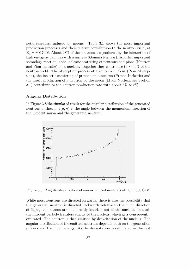
netic cascades, induced by muons. Table 3.1 shows the most importantproduction processes and their relative contribution to the neutron yield, atEµ = 300 GeV. About 28% of the neutrons are produced by the interaction ofhigh energetic gammas with a nucleus (Gamma Nuclear). Another importantsecondary reaction is the inelastic scattering of neutrons and pions (Neutronand Pion Inelastic) on a nucleus. Together they contribute to ∼ 49% of theneutron yield. The absorption process of a π− on a nucleus (Pion Absorp-tion), the inelastic scattering of protons on a nucleus (Proton Inelastic) andthe direct production of a neutron by the muon (Muon Nuclear, see Section3.1) contribute to the neutron production rate with about 6% to 8%.

Angular Distribution

In Figure 3.8 the simulated result for the angular distribution of the generatedneutrons is shown. θ(µ, n) is the angle between the momentum direction ofthe incident muon and the generated neutron.

Figure 3.8: Angular distribution of muon-induced neutrons at Eµ = 300 GeV.

While most neutrons are directed forwards, there is also the possibility thatthe generated neutron is directed backwards relative to the muon directionof flight, as neutrons are not directly knocked out of the nucleus. Instead,the incident particle transfers energy to the nucleus, which gets consequentlyexcitated. The neutron is then emitted by deexcitation of the nucleus. Theangular distribution of the emitted neutrons depends both on the generationprocess and the muon energy. As the deexcitation is calculated in the rest

37

frame, the neutron momentum has to be lorentz-transformed to the labora-tory frame.

3.5 Neutron Propagation into the Detector

Figure 3.9: Schematic cross section through the LENA detector, the samecolour codes as in Figure 3.3 apply. For the simulation only neutrons gener-ated in the grey region were considered.

The starting point of the neutron was chosen randomly in a 1.96 m thickcylinder around the muon veto (see Figure 3.9). Previous simulations haveshown that neutrons which were produced farther away from the detector donot need to be considered, as the majority will be absorbed in the rock be-fore they reach the detector. The neutron energy and momentum directionwas chosen randomly according to the previously simulated neutron spec-trum. Only neutrons with E > 40 MeV were simulated, as the range of lowerenergetic neutrons is too small to reach the target volume. Neutron tracksthat pointed away (2π solid angle) from the detector were also not followed,as previous simulations have shown that the chance that these neutrons arebackscattered and reach the detector is with ∼ 2% negligible. Secondaryneutrons were also followed in the simulation. In the case of multiple neu-trons, the stopping point of the neutron reaching the smallest radius waschosen.20 million neutrons above 40 MeV were simulated using the energy spectrumand angular distribution corresponding to a muon mean energy of 300 GeV(4 km w.e.). Assuming that all tracks are perfectly vertical, the muon rateon this 226 m2 area is 1.45·10−2 s−1 at 4 km w.e. depth. Using the results

38

Figure 3.10: Simulated range of muon-induced fast neutrons in LENA, withPXE used as scintillator and buffer liquid. Additionally, an exponential fitis plotted. The red region represents the neutrons that reached the targetvolume. Statistics corresponds to ∼ 15 years at 4 km.w.e. depth.

from the previous simulation (see Section 3.4), ∼ 1.3 · 106 neutrons per yearwith E > 40 MeV are produced in the mantle. Thus, the statistics of thesimulation corresponds to ∼ 15 years.Figure 3.10 shows the simulated range of muon-induced neutrons in LENAusing PXE as scintillator and buffer liquid. The minimal radius of a neutrontrack’s end point is ∼ 6 m, which is far inside the target volume, and manyneutrons reach the target volume. The neutron range can be fitted with anexponential function a · e rλ , where a is a constant factor, λ is the mean freepath and r is the radius of the neutron track’s end point. In PXE the meanfree path length λ is 0.676 ± 0.005 m and in LAB it is 0.687 ± 0.006 m. Forcomparison, in the LVD experiment a mean free path length of 0.634±0.012 mwas measured, with a different scintillator (C10H20) [53]. Between r ∼ 13 mand r ∼ 15 m the fit describes the simulated neutron range very good, butbelow r ∼ 13 m the fit function decreases faster with the radius than thesimulated neutron range. If the fit range is constricted from 9 m to 13 mthe mean free path length increases in PXE to 0.778± 0.016 m. The reasonfor this characteristic is that the neutrons are not monoenergetic and thatthe mean free path length increases with the energy. Therefore, the averageneutron energy increases with the distance to the muon track as well as theaverage mean free path length.The inital energy spectrum of the neutrons that reached the target volume

39

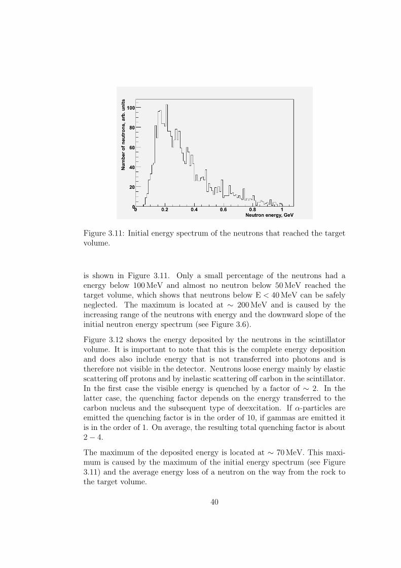
Figure 3.11: Initial energy spectrum of the neutrons that reached the targetvolume.

is shown in Figure 3.11. Only a small percentage of the neutrons had aenergy below 100 MeV and almost no neutron below 50 MeV reached thetarget volume, which shows that neutrons below E < 40 MeV can be safelyneglected. The maximum is located at ∼ 200 MeV and is caused by theincreasing range of the neutrons with energy and the downward slope of theinitial neutron energy spectrum (see Figure 3.6).

Figure 3.12 shows the energy deposited by the neutrons in the scintillatorvolume. It is important to note that this is the complete energy depositionand does also include energy that is not transferred into photons and istherefore not visible in the detector. Neutrons loose energy mainly by elasticscattering off protons and by inelastic scattering off carbon in the scintillator.In the first case the visible energy is quenched by a factor of ∼ 2. In thelatter case, the quenching factor depends on the energy transferred to thecarbon nucleus and the subsequent type of deexcitation. If α-particles areemitted the quenching factor is in the order of 10, if gammas are emitted itis in the order of 1. On average, the resulting total quenching factor is about2− 4.

The maximum of the deposited energy is located at ∼ 70 MeV. This maxi-mum is caused by the maximum of the initial energy spectrum (see Figure3.11) and the average energy loss of a neutron on the way from the rock tothe target volume.

40

Figure 3.12: Total energy deposited by neutrons in the scintillator volume ofLENA. The effective visible energy will be quenched by a factor of ∼ 2− 4.

3.6 Background Rates in LENA

Table 3.2 shows the resulting neutron background rates in LENA at 4 km w.e.depth, as a function of the fiducial volume with PXE used as scintillator sol-vent. The neutron background rates in LENA with LAB used as scintillatorsolvent are shown in Table 3.3. Around 170 neutrons per year reach thetarget volume in PXE, in LAB this rate increases to ∼ 200 per year. Be-cause the density of PXE (ρPXE = 985 g

l) is greater than the density of LAB

(ρLAB = 860 gl) the self-shielding effect of PXE is larger. The neutron back-

ground rate is therefore higher in LAB.

The difference in neutron background rate between the two solvents increaseswith the shielding. While the neutron background rate is only ∼ 20% largerfor LAB if the fiducial volume radius is set to 13 m, it is ∼ 90% larger if thefiducial volume has a radius of 10 m.

Table 3.2 and 3.3 also include the event numbers in two energy bins cor-responding to the geoneutrino and DSNB detection windows, respectively.Considering the possible range in quenching factors (see Section 3.5), adeposited energy of 2 MeV - 9.6 MeV corresponds to a visible energy be-tween 1.8 MeV and 3.2 MeV in which the geoneutrino signal is expected.The 10 MeV - 25 MeV DSNB detection window corresponds to a depositedneutron energy between 20 MeV and 100 MeV.

As about 1000 geo-ν events per year are expected in LENA, fast neutronsprovide a negligible background for the geoneutrino detection.

41

Fiducial Volume Number of neutrons [/y]Radius [m] Total energy range Geo-ν-region DSNB-region

13 166 5.2 7012 54 0 1411 15 0 1.710 3.9 0 0.39 0.9 0 0.1

Table 3.2: Neutron background rates per year in LENA as a function of thefiducial volume radius with PXE as scintillator solvent. The Geo-ν-regioncorresponds to 2 MeV < En < 9.6 MeV, the DSNB region to 20 MeV < En <100 MeV, due to the neutron quenching.

Fiducial Volume Number of neutrons [/y]Radius [m] Total energy range Geo-ν-region DSNB-region

13 200 6.2 8312 69 0 1811 21 0 2.710 7.4 0 0.59 2.8 0 0.1

Table 3.3: Neutron background rates per year in LENA as a function of thefiducial volume radius with LAB as scintillator solvent. The Geo-ν-regioncorresponds to 2 MeV < En < 9.6 MeV, the DSNB region to 20 MeV < En <100 MeV, due to the neutron quenching.

42

The situation is quite different for the detection of the DSNB, as the back-ground rate in the DSNB-region is much greater, and the expected signalis much smaller (6-13 events per year). If the neutron background can notbe reduced, the radius of the fiducial volume needs to be set to 10 m, toachieve a signal-to-background (S/B) ratio of better than 10:1. This wouldmean that more than 40% of the target volume would be lost. In this case,the remaining neutron background in LAB would be ∼ 60% higher than inPXE. Thus, from the aspect of neutron background, PXE is the preferredscintillator.Another possibility is to increase the water shielding around the buffer. In thepre-design study for the Pyhasalmi location [22], the water Cerenkov muonveto has a elliptically shape with at least 2 m shielding. Due to this geometry,the effective shielding would be larger than the 2 m that were assumed in thissimulation. The presented results are therefore a conservative estimation.Nevertheless, they show that the muon-induced neutron background is acentral issue for the detection of rare events like the DSNB, in LENA.

3.7 Identification of Neutron Events

As neutron interactions in the scintillator differ from those of a positronemitted in the inverse beta decay reaction, it might be possible to distinguishneutron from νe events by the use of special discrimination criteria. Depend-ing on the efficiency of the methods used, the fast neutron background couldbe reduced considerably.

3.7.1 Multiple Neutron Capture Events

If a muon-induced neutron enters the scintillator volume, it can generatesecondary neutrons by inelastic scattering off carbon. Like the primary neu-tron, these secondary neutrons are captured on free protons and are thuseasily detected (see Figure 3.13). Due to the kinematics of the reaction, aneutron from an inverse-beta decay reaction has not enough energy to gen-erate secondary neutrons. Therefore, events with more than one neutroncapture signal within 1 ms (corresponding to ∼ 5 times the capture time of aneutron in common liquid scintillators) can be rejected as fast neutrons. Inprinciple it is possible that a DSNB-event is misidentified as a fast neutronevent, through random coincidence due to intrinsic radioactivity. But as thetime window around the potential DSNB-event is with 1 ms very short andthe radioactive purity level of LENA will be very high, the probability forrandom coindicences is negligible.

43

Figure 3.13: Simulated photon signal of a neutron event, where a secondaryneutron was generated. The signal of the two capture processes is clearlyseperated which allows to distinguish this event from a νe event.

The neutron background rates after application of the neutron capture cutare shown in Table 3.4 for PXE and Table 3.5 for LAB as scintillator solvent.The efficiency of this method depends on the neutron energy, as higher-energetic neutrons are more likely to produce secondary neutrons. Since theaverage energy of a neutron increases with the shielding, the efficiency ofthis method depends on the fiducial volume radius. For the smallest fiducialvolume, a neutron background rejection efficiency of ∼ 60% can be achievedwith this method.

3.7.2 Pulse Shape Analysis

The light decay curve caused by a particle interacting in a liquid scintillatordepends on its energy deposition per unit path length (dE

dx) and thus on the

particle mass and charge. This allows the discrimination of different particlesby pulse shape analysis (see Figure 3.14).The probability density function (PDF) F(t) of the photon emission processin liquid scintillator can be described by the sum of several exponential decays[15]:

F (t) =∑i

Ni

τi· e−

tτi (3.4)

where τi is the decay time constant of the exponential function i and Ni its

44

Number of neutrons [/y]Fiducial Volume Total 20 MeV < En < 100 MeV

Radius [m] energy range DSNB-region13 95 5012 21 8.911 4.5 1.110 1.2 0.29 0.3 0.1

Table 3.4: Neutron background rates per year in LENA as a function of thefiducial volume radius, with PXE as scintillator solvent and applying a mul-tiple neutron capture veto. The indicated neutron energy region correspondsin visible energy to the DSNB detection window.

Number of neutrons [/y]Fiducial Volume Total 20 MeV < En < 100 MeV

Radius [m] energy range DSNB-region13 119 6212 28 1211 6.9 1.910 2.2 0.49 0.7 0.1

Table 3.5: Neutron background rates per year in LENA as a function of thefiducial volume radius, with LAB as scintillator solvent and applying a mul-tiple neutron capture veto. The indicated neutron energy region correspondsin visible energy to the DSNB detection window.

45

relative contribution to the PDF (such that∑

iNi = 1). The exponentialfunction with the shortest decay time constant is usually referred to as thefast component, the other exponential functions are the so-called slow com-ponent. Heavier particles have a larger ratio between the slow and the fastcomponent of the PDF than lighter particles. Typically 60% to 80% of thephotons are emitted by the fast component, the exact value depends on theparticle type and the scintillator. The fast time constant is usually in theorder of 2 ns to 5 ns, the slow time constants are in the range of 10 ns to200 ns.Neutrons generate scintillation light only indirectly by elastic scattering offprotons and inelastic scattering off carbon, where amongst others gammas,protons and α-particles are produced. As the neutron looses its energy inseveral elastic and inelastic scattering processes, it is possible to get doublepeak structures if the time difference between two scattering processes is ofthe order of several ns or more. Consequently, neutrons feature a differentpulse shape than positrons generated in inverse beta decay reactions. Thisshould allow pulse shape discrimination of neutron and νe events. A detailedanalysis for LENA will be presented in Chapter 5.

Figure 3.14: Comparison of the typical pulse shapes for α-particles, protonsand electrons in liquid scintillator [15]

46

Chapter 4

Neutron-Gamma Pulse ShapeDiscrimination in LiquidScintillators

It was shown in Chapter 3 that muon-induced neutrons provide a back-ground for the detection of rare νe events in LENA. A possible way toreduce this background is to discriminate neutron from νe events by pulseshape analysis (see Section 3.7.2). Therefore, an experiment was performedin which the efficiency of a neutron-gamma pulse shape discrimination in asmall liquid-scintillator detector was examined. The results were comparedto a simulation of the same setup in order to determine the necessary scin-tillation parameters. In the following, these values could be transferred tothe GEANT4 simulation of LENA to investigate pulse shape discrimination(see Chapter 5).

4.1 Tail-to-total Discrimination Method

In a liquid-scintillator detector, the typical pulse shape depends on the parti-cle type (see Section 3.7.2). The ratio between the slow and the fast compo-nent of the probability density function (PDF) is larger for heavier particles.

In the tail-to-total discimination method the photon signal is integrated overtwo different time intervals. One interval encompasses the complete pulse,while the other interval encompasses only the last part of it, the so-called tail(see Figure 4.3). Then the ratio between the ”total” and the ”tail” intervalis calculated [16]. Based on the PDF (see equation (3.4)) of the photon

47

emission process, the tail-to-total ratio R is defined as:

R =∑i

Nie− tτi (4.1)

where t is the start time of the ”tail” interval.As the amplitudes Ni depend on the particle type, the tail-to-total ratio ischaracteristical for the particle type. Heavier particles have a higher tail-to-total ratio than lighter particles, as the contribution of the slow componentto the PDF is larger (see Figure 3.14). Thus, a discrimination between twoparticle types is possible by the comparison of the tail-to-total ratios.

4.2 Experimental Setup

The experiment was setup at the MLL (Maier-Leibniz-Laboratorium) in thetandem accelerator building in Garching. The setup consists of a hexagonallyshaped container filled with liquid scintillator that is coupled directly to aPhilips XP 3461 B PMT via a perspex window. The container is 50 mm highand its radius is 45.5 mm. As it is coupled directly to the PMT on one side,the optical coverage is approximately 23% (see Figure 4.1).

Figure 4.1: Schematic experimental setup. The Am-Be source emits neutronsand gammas, which generate light in the liquid scintillator sample. Thescintillation light is detected by the PMT, which is coupled directly to theliquid scintillator.

48

An Am-Be source is used, as it emits both neutrons and gamma rays. 241Amis an α-emitter with 432.2 years half-life. The α-particle is subsequentlycaptured on a 9Be nucleus, resulting in the emission of a neutron and agamma quantum:

α +9 Be→13 C∗ →12 C + n+ γ (4.2)

The emitted neutrons have a continious spectrum up to 10 MeV with 5 MeVmean energy (see Figure 4.2). The energy of the emitted gamma quantumis 4.44 MeV, corresponding to the first excited state of 12C [54].

Figure 4.2: Energy spectrum of the neutrons emitted by the Am-Be source.The mean neutron energy is 5 MeV [55].

Two liquid scintillators were used in this experiment. PXE1(phenyl-xylyl-ethane) and LAB2 (linear alkylbenzene), both with 10 g

lPPO (2,5-diphenyl-

oxazole). The typical pulse shape depends on the PPO concentration, butbetween 2 g

land 10 g

lthe differences are rather small for both PXE and LAB

[15].

Due to the small volume of the liquid scintillator sample, the majority ofneutrons and gammas scatter off only once in it.

1Produced by Dixie Chemical Co., Houston TX (US)2Produced by Petresa Canada, part of CEPSA Group, Becancour QC(CDN)

49

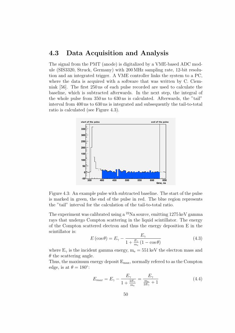
4.3 Data Acquisition and Analysis

The signal from the PMT (anode) is digitalized by a VME-based ADC mod-ule (SIS3320, Struck, Germany) with 200 MHz sampling rate, 12-bit resolu-tion and an integrated trigger. A VME controller links the system to a PC,where the data is acquired with a software that was written by C. Ciem-niak [56]. The first 250 ns of each pulse recorded are used to calculate thebaseline, which is subtracted afterwards. In the next step, the integral ofthe whole pulse from 350 ns to 630 ns is calculated. Afterwards, the ”tail”interval from 400 ns to 630 ns is integrated and subsequently the tail-to-totalratio is calculated (see Figure 4.3).

Figure 4.3: An example pulse with subtracted baseline. The start of the pulseis marked in green, the end of the pulse in red. The blue region representsthe ”tail” interval for the calculation of the tail-to-total ratio.

The experiment was calibrated using a 22Na source, emitting 1275 keV gammarays that undergo Compton scattering in the liquid scintillator. The energyof the Compton scattered electron and thus the energy deposition E in thescintillator is:

E (cos θ) = Eγ −Eγ

1 + Eγme

(1− cos θ)(4.3)

where Eγ is the incident gamma energy, me = 551 keV the electron mass andθ the scattering angle.Thus, the maximum energy deposit Emax, normally refered to as the Comptonedge, is at θ = 180◦:

Emax = Eγ −Eγ

1 + 2Eγme

=Eγ

me2Eγ

+ 1(4.4)

50

For Eγ = 1275 keV, the maximum recoil energy is Emax=1062 keV.In the spectrum recorded of the 22Na source, the known energy at the Comp-ton edge can be used to determine the relation between the integral of thesignal and the energy deposited (see Figure 4.4).As the deposited energy is proportional to the integrated signal s, it can bedetermined from the latter by the following equation:

E = s · 1062 keV

scompton edge(4.5)

Figure 4.4: Calibration of the experimental setup with PXE used as liquidscintillator. The energy resolution ∆E

Eis proportional to 1√

N, where N is the

number of registered photons in the PMT, and the gamma quant scattersonly once in the detector. Thus, the Compton egde of 22Na gamma rays, at1062 keV, is fitted with a Gauss function, in order to determine the relationbetween the integral of the signal and the deposited energy

4.4 Results

Figure 4.5 shows the tail-to-total ratio of the measured pulses with PXEused as liquid scintillator and an energy threshold of 1 MeV. The gammaand neutron events seperate into two peaks that have a small overlap. Asthe Compton scattered electrons feature a lower charge-to-rest-mass ratiothan the recoil protons from neutron scattering, the left peak in Figure 4.5belongs to gamma events and the right one to neutron induced events. Eachpeak can be fitted with a Gaussian:

N · 1

σ√

2π· e−

(x−µ)2

2σ2 (4.6)

51

Figure 4.5: Tail-to-total ratios of the measured pulses in PXE. The energythreshold was set to 1 MeV. The two peaks from gamma (left peak) andneutron (right peak) events are clearly seperated, such that 99.5% of theneutron events can be rejected, if 97.8% of the gamma events are accepted.Each peak was fitted with a Gaussian function (the corresponding sum ofboth functions is shown here).

where N is the number of events, µ is the expected value and σ is the standarddeviation. The resulting fit values for the gamma peak are µγ = (8.6 ±0.017) · 10−2, σγ = (1.0 ± 0.012) · 10−2, and µn = 0.16 ± 2.4 · 10−4, σn =(1.7± 0.019) · 10−2 for the neutron peak, respectively.The separation efficiency between the two peaks can be described by thepeak distance parameter parameter D:

D =µn − µγ√σ2n + σ2

γ

(4.7)

which denotes the distance between the two peaks, in terms of the meanstandard deviation

√σ2n + σ2

γ.Thus, the distance between the gamma and the neutron peak in Figure 4.5is D=3.87. If one accepts only events with a tail-to-total ratio that is smallerthan µγ + 2σγ, 97.8% of all gamma events are accepted, while 99.5% of allneutron events are rejected. Almost all neutron are identified, losing only2.2% of gamma events to false identification.The peak distance D between the gamma and the neutron peak and the cor-responding efficiencies of the neutron-gamma discrimination were calculatedfor five different energy intervals between 0.5 MeV and 3.5 MeV visible en-ergy. The resulting energy dependence of the distance D is shown in Figure

52

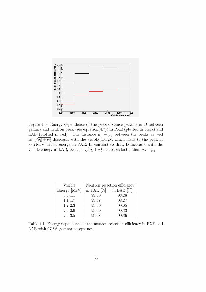
Figure 4.6: Energy dependence of the peak distance parameter D betweengamma and neutron peak (see equation(4.7)) in PXE (plotted in black) andLAB (plotted in red). The distance µn − µγ between the peaks as wellas√σ2n + σ2

γ decreases with the visible energy, which leads to the peak at∼ 2 MeV visible energy in PXE. In contrast to that, D increases with thevisible energy in LAB, because

√σ2n + σ2

γ decreases faster than µn − µγ.

Visible Neutron rejection efficiencyEnergy [MeV] in PXE [%] in LAB [%]

0.5-1.1 99.80 93.281.1-1.7 99.97 98.271.7-2.3 99.99 99.052.3-2.9 99.99 99.332.9-3.5 99.98 99.36

Table 4.1: Energy dependence of the neutron rejection efficiency in PXE andLAB with 97.8% gamma acceptance.

53

4.6 for PXE and LAB. The corresponding efficiencies of the neutron-gammadiscrimination is shown in Table 4.1.As the tail-to-total ratio depends on the energy deposition per unit pathlength dE

dx, µn,γ depends on dE

dxof the recoil proton and the recoil electron,

respectively. For electrons, the energy dependence of dEdx

is insignificant be-tween 0.5 MeV and 3.5 MeV [57]. But the energy loss dE

dxof the protons

decreases with the proton energy in the relevant energy region [57]. Thus,the distance µn − µγ between the neutron and the gamma peak decreaseswith energy.But σ2

n,γ decreases also with the energy deposited, because the enlarged num-ber of photons minimizes the statistical fluctuations around the ideal PDF.In LAB, this effect is strong enough to compensate the decreasing distancebetween the gamma and the neutron peak with rising energy. Therefore,the efficiency of the neutron-gamma discrimination increases with the visibleenergy in LAB.In PXE the peak distance D gets maximal at Evisible ∼ 2 MeV and then startsto decrease, because the distance between the peaks µn−µγ decreases fasterthan

√σ2n + σ2

γ.The efficiency of the neutron-gamma discrimination is higher in PXE thanin LAB (see Table 4.1). Nevertheless, in both scintillators more than 99% ofthe neutron events with a visible energy between 2 MeV and 3.5 MeV can berejected with a 97.8% acceptance of the gamma events.

4.5 Monte Carlo Simulation

Besides the measurements, the experiment was reproduced with the sameprogram used for the simulation of the fast neutron background (see Section3). The simulated detector geometry consists of a 50 mm high cylinder with91 mm in diameter, which is filled with PXE or LAB. Every photon thathits the walls of the cylinder is counted and the time of the hit is saved. Inthe simulation an effective light yield was used, which is determined by thephysical light yield (∼ 10000 photons per MeV), the optical coverage ∼ 23%and the quantum efficiency of the PMT ∼ 20% [15]. The best reproductionof the measured data could be achieved with an effective light yield of 440photons per MeV for PXE and 370 photons per MeV for LAB.Scattering and absorption processes were also included in the simulation.The Rayleigh scattering length and absorption length were set 20 m for bothscintillators. Therefore, the effects of both processes should be negligible.The proton quenching was described by the Birks formula (see equation(3.2)), setting kb = 0.15 mm

MeVfor both PXE and LAB [58].

54

A time jitter of 3 ns was added to the hit time of the photon, in order tosimulate the time resolution of the PMT that was used in the experiment.A PDF F(t) featuring two decay terms was assumed for the scintillationemission:

F (t) =Nf

τfe− tτf +

Ns

τse−

tτs (4.8)

Nf,s denotes the probability that a scintillation photon is emitted by the fastand slow component, respectively, and τf,s are the corresponding decay timeconstants. For PXE, τf was set to 2.9 ns and τs was set to 29 ns and for LAB,τf was set to 3.7 ns and τs was set to 31 ns, as these values were derived froma fit of the average pulses recorded in the experiment (for comparison, τfwas determined to ∼ 2 ns for both PXE and LAB in [15] using a PDF with4 exponential functions).The value of Nf depends on the particle type and for protons also on theenergy. For electrons, it was set to 0.8 for PXE and to 0.72 for LAB (thesevalues were also derived from a fit of the average pulses recorded in theexperiment).The energy dependence of the measured tail-to-total ratio for protons can befitted with the sum of an exponential function and a constant function (seeFigure 4.7). As the tail-to-total ratio is defined by:∑

i

Nie− tτi

t�τf≈ Nse

− tτs (4.9)

it is proportional to Ns. Thus, as τs is energy independent, the energy de-pendence of Ns and Nf can also be described by the sum of an exponentialand a constant function:

Nf = p0 + p1 · ep2·Evis (4.10)

where p0, p1 and p2 are scintillator dependent parameters, and Evis is thevisible energy.For PXE Nf was calculated by

Nf = 0.744− 0.12 · e−0.00054

keV·Evis (4.11)

and for LAB by

Nf = 0.6895− 0.086 · e−0.0003

keV·Evis (4.12)

because with these values for p0, p1 and p2 an optimal reproduction of theexperimentally measured tail-to-total ratio was achieved.The simulation was calibrated in the same way as the experimental setup(see Section 4.3).

55

Figure 4.7: Measured energy dependence of the tail-to-total ratio for neutronsin PXE. A fit based on the sum of an exponential and a constant function(p0 + p1 · ep2·Evis) is shown.

2·105 gamma particles with Eγ=4.44 MeV and 2·105 neutrons with En =10 MeVwere simulated for each scintillator. For the calculation of the tail-to-totalratio the start of the ”tail” interval was set to 15 ns.

The reproduced values for σn,γ were smaller than the measured ones, becauseeffects of the PMT and electronics that influence the experimental resultare not reproduced in the simulation. Pre- and afterpulses of the PMTare omitted, and the start time of the pulse is always determined perfectly.Thus a systematic error was added to the tail-to-total ratio to compensatethe lack of these error sources. An optimal reproduction was achieved whenthe systematic error was set to σ = 4 · 10−3.

As for the experimental data, the distribution of the tail-to-total ratio wasfitted with the sum of two Gauss functions, for reproducing the neutron andgamma peaks.

The resulting simulated energy dependence of the distance D between thegamma and the neutron peak is shown in Figure 4.8 for PXE and in Figure4.9 for LAB.

The simulated peak distance D differs from the experimentally measured oneby 2% to 10%, depending on the visible energy. The decrease of the peakdistance D in PXE above ∼ 2 MeV is reproduced by the simulation, witha small difference in the exact energy dependence of D. As no backgroundsources are simulated, σγ,n shows a slightly different energy dependence in thesimulation. These are probably caused by the neglection of electronics effectsin the simulation. As a good agreement between the experimental and the

56

Figure 4.8: Simulated energy dependence of the peak distance parameterD between gamma and neutron peak (see equation(4.7)) with PXE usedas scintillator. The dashed line shows the experimental results. The peakat ∼ 2 MeV visible energy is reproduced by the simulation. Overall thesimulated peak distance differs from the experimentally measured one by2%-10%, depending on the visible energy.

Figure 4.9: Simulated energy dependence of the peak distance parameter Dbetween gamma and neutron peak (see equation(4.7)) with LAB used as scin-tillator. The dashed line shows the experimental results. The simulated peakdistance differs from the experimentally measured one by 3%-7%, dependingon the visible energy

57

simulated results is achieved, a simulation of the pulse shape discriminationbetween fast neutron and νe events in LENA should obtain realistic results.The results of this simulation will be presented in Chapter 5.

58

Chapter 5

Pulse Shape Discrimination ofNeutron and νe Events inLENA

The capability to distinguish neutron events from gamma events in a smallliquid-scintillator detector by pulse shape analysis was demonstrated in Chap-ter 4. At visible energies between 2 MeV and 3.5 MeV, neutron rejection atan efficiency level of more than 99% was reached, while a gamma acceptanceof 97.8% remained.

In this Chapter the results of a Monte Carlo simulation will be presentedthat has analyzed the efficiency of a pulse shape discrimination between fastneutrons and νe events in LENA. As LENA is a 50 kt detector, absorptionand scattering of the scintillation light becomes important. Light propagationeffects could be neglected in the experiment described in Chapter 4, becauseof the small detector volume. Moreover, the neutron normally deposits itscomplete energy in the LENA scintillator volume by multiple scatteringprocesses, which has an effect on the pulse shape. Finally, in LENA thepulse shape discrimination has to be applied at significantly higher visibleenergies of 10 MeV to 25 MeV in the DSNB detection region.

5.1 Simulation Setup

The LENA detector setup is the same as explained in Section 3.3.1. Thesame scintillation properties as in Section 4.5 are used (see Table 5.1), theRayleigh scattering and absorption length are set to 20 m for both PXE andLAB and the time resolution of the PMTs is set to 1 ns.

As no experimental data was availabe for Nf of α-particles at higher energies

59

PXE LABτf 2.9 ns 3.7 nsτs 29 ns 31 nsNf 0.8 0.72

Nf (p, α) 0.744− 0.12 · e−0.00054keV

·Evis 0.6895− 0.086 · e−0.0003keV

·Evis

kb 0.15mm/MeV 0.15mm/MeV

Table 5.1: Scintillation properties for LAB and PXE. Nf (p, α) denotes thefraction of photons that are emitted by the fast component when an α-particleor a proton deposites energy, Nf is applied for all other particles.

in PXE and LAB, it is set to the same energy dependent value as Nf ofprotons, which was determined in Section 4.5. This conservative estimateshould lead to a smaller discrimination efficiency, as the real value of Nf islower for α−particles than for protons (see Figure 3.14). However, it shouldhave small effect on the average neutron pulse shape, as α−particles are onlycreated in neutron induced spallation reactions.

A further modification arises by the difference in the time of flight for in-dividual photons. The distance from the origin of a scintillation photon tothe PMT where it is finally detected, depends on its initial position and itsmomentum direction. For example, for a photon that is emitted at a radiusof 10 m and z=0 m in the target volume (the z-axis is the symmetry axis ofthe cylinder, z=0 denotes the center of the cylinder), the shortest distanceto a PMT is 5 m and the farthest distance is more than 50 m. This causesa difference in the detection time of two photons that were emitted at thesame time, but with a different momentum direction. As the photons areemitted isotropically, this has a great impact on the combined pulse shaperecorded by all PMTs (see Figure 5.1). Thus, it is necessary to subtract theso-called time of flight that a photon needs to get from its emission pointto its detection point. This is, of course, only possible if there is a preciseevent position reconstruction method. First Monte Carlo simulations showedthat position reconstruction with an uncertainty σ < 20 cm at a visible en-ergy above 10 MeV is possible in LENA [29]. Therefore, for every photondirection the time of flight was calculated with a time jitter of 1 ns (corre-sponding to σ ≈ 20 cm with a refractive index n=1.56), in order to includethe uncertainty of the position reconstruction.

60

Figure 5.1: Comparison of the average pulse shape with (plotted in black)and without (plotted in red) time of flight correction in LENA for a 10 MeVpositron at r=10 m and z=0. Without time of flight correction, less photonsare detected in the first 10 ns of the events and more afterwards. There isalso an additional peak at ∼ 100ns when the photons that were emittedtowards the center of LENA are detected on the other side of the steel tank.

5.2 Results

The majority of the fast neutrons that reach the target volume from outsidewill be stopped at a radius of r=10 m or more (see Figure 3.10).

Thus, for all simulated neutrons and positrons the particle origin was setto radius r=10 m and z=0 m, as the fast neutron events are expected atlarger radii (see Figure 3.10). The neutron energy was set to 2.3 times thepositron energy, as the average neutron quenching factor is 2.3. Neutrons andpositrons were simulated at different energies corresponding to an interval ofvisible energy between 10 MeV and 25 MeV (DSNB energy window see Sec-tion 2.2.3). Neutron events can easily be identified, if secondary neutrons areproduced, by the additional 2.2 MeV gamma peak from the neutron captureon a proton (see Section 3.7.1). Therefore, neutron events are only includedin this analysis, if no secondary neutrons were produced.

As it can take up to a few ns before a neutron generates scintillation lightby elastic scattering off protons or inelastic scattering off carbon, the starttime of the pulse had to be determined by a constant fraction method. Thephoton hit times were written into a ROOT histogram with 1 ns binning andthe maxinum of entries in a single bin Nmax was calculated. The first bin

61

with more than 0.05 · Nmax entries was considered as the start of the pulse.For the calculation of the tail-to-total ratio, the start of the ”tail” intervalwas set to 15 ns after the beginning of the pulse.

Figure 5.2 shows the tail-to-total ratio of 25000 neutron and 25000 positronevents with 10 MeV visible energy in PXE.

Figure 5.2: Tail-to-total ratio of positrons (plotted in red) and neutrons(plotted in black) with 10 MeV visible energy in PXE. With 95% positronacceptance 99.40± 0.05% of the neutron events can be rejected.

The neutron and the positron peaks are clearly seperated. If 95% of thepositron events are accepted, 99.40 ± 0.05% of the neutron events can berejected.

The greater width of the neutron distribution in Figure 5.2 compared tothe positron peak has several reasons. As the neutron interacts by varyingprocesses (elastic scattering off protons and inelastic scattering off carbon),the neutron peak is widened due to different secondary particles. Moreover,the neutron deposits its energy in multiple scattering processes. It is possiblethat several ns pass after the first interaction before the neutron scatters asecond time. This leads of course to a greater tail-to-total ratio, as thebeginning of the tail interval is set relative to the first scattering process.Hence, the neutron tail-to-total ratio shows an asymmetry to higher values.It is therefore not possible to fit the neutron tail-to-total ratio with a singleGaussian function.

The positron peak also shows a slight asymmetry to higher values. Thereason for this characteristic is that the positron will in some cases annihilate

62

with an electron into two gamma quanta before it is stopped. This changesthe signal time structure as the gamma quanta need some time to Comptonscatter off electrons and thus, the emission of some of the scintillation lightis delayed which leads to a higher tail-to-total ratio.

The energy dependence of the neutron-positron discrimination for visibleenergies between 10 MeV and 25 MeV is shown in Figure 5.3 for both PXEand LAB.

Figure 5.3: Energy dependence of the efficiency of the neutron rejection forPXE (black markers) and LAB (red markers) with 95% positron acceptance.

With 95% positron acceptance, between 99.4% and 99.8% of the neutronevents can be rejected in PXE, depending on the visible energy. In LAB, thediscrimination efficiency is as expected from the neutron-gamma discrimina-tion in a small detector worse (see Section 4.4), but with 99.0%-99.5% stillvery good. As expected, the discrimination efficiency in PXE increases withenergy, as the measurement of the tail-to-total ratio gets more precise dueto the increasing number of scintillation photons. LAB shows a similar en-ergy dependence up to 20 MeV of visible energy, but then the discriminationefficiency starts to decrease. The reason for this effect is that the distance be-tween the positron and the scattered proton peak is still decreasing in LAB,while it is almost constant in PXE at visible energies above 10 MeV (accord-ing to the energy dependence of Nf(p, α) that was determined in Chapter4, see Table 5.1). Above 20 MeV visible energy, this decrease is not com-pensated by the increasing number of scintillation photons anymore, whichcauses the decline of neutron-positron discrimination efficiency.

63

For both LAB and PXE, the efficiency of the neutron-positron discriminationin LENA is lower as the efficiency of the neutron-gamma discrimination atlower energies in a small detector (see Section 4.4). One reason for thisis, that by inelastic neutron scattering off carbon, gammas can be emitted,which Compton scatter off electrons and have nearly the same pulse shapeas positrons. In LENA all produced gamma quanta will be detected due tothe large target mass, while in a small detector the gamma quanta will leavethe detector without further interaction.Another factor which leads to a worse discrimination is the scattering of pho-tons, which is important in LENA due to the large detector dimensions. If aphoton is scattered off, its track length between the emission and detection islonger than is it assumed in the calculation of the time of flight and thereforeits detection time is increased. Thus, more photons are detected in the tailinterval (see Figure 5.4 for a comparison of the average positron pulse shapewith 20 m scattering length and a hypothetical scattering length of 20 kmin LENA). As photons emitted due to the fast PDF component are nowdetected in the tail interval originally dominated by the slow component, theefficiency of the neutron positron is decreased. Simulations show that with-out scattering, the discrimination efficiency at 10 MeV visible energy wouldincrease from 99.40± 0.05% to 99.85± 0.03% in PXE.

64

Figure 5.4: Average pulse shape of 10 MeV positrons in PXE with 20 mscattering length (plotted in black) and a hypothetical scattering length of20 km (plotted in red), such that the scattering of photons is negligible. Ifa photon is scattered off, the real track is longer than the assumed one forthe time of flight calculation. Thus, more photons are detected in the tailinterval after 15 ns for the realistic value of 20 m scattering length than forthe hypothetical 20 km scattering length.

65

66

Chapter 6

Cosmogenic Background forthe DSNB Detection

As only 6 to 13 DSNB events per year are expected in LENA [18], back-ground is a central issue for the DSNB detection. There are three cosmogenicbackground sources. Muons produce βn-emitting radioisotopes in the scin-tillator, like 8He or 9Li, by spallation reactions on carbon in the scintillator,which have the same signature as νe events. As the detection window for theDSNB is above 10 MeV, due to the reactor νe spectrum, only 9Li has a largeenough Q-value to add to the background. Another source are fast neutrons,because they give a prompt signal due to scattering off protons and carbon,and a delayed signal caused by the neutron capture on a free proton. Theyare generated by cosmic muons in the surrounding rock and propagate intothe detector. Lastly, atmospheric neutrinos provide an intrinsic backgroundand can also produce neutrons by neutral current spallation reactions oncarbon in the detector.

In the following analysis, a muon flux of ΦLµ = 6.5 · 10−5m−2s−1 and a mean

muon energy of 〈ELµ 〉 = 300 GeV is assumed, corresponding to 4 km w.e.

shielding [45].

6.1 9Li In-situ Production

The maximum energy for the 9Li-βn-decay branch is with 11.3 MeV in thelower end of the DSNB detection region [12]. A shift of the lower thresholdabove 11.3 MeV would be possible, but is not favorable as the expected DSNBflux is maximal around 10 MeV (see Figure 2.6) and thus, a lot of eventswould be lost. The cosmogenic 9Li production rate was measured by theKamLAND experiment. Above 8.3 MeV the observed rate for 1 kt target

67

mass was RK9Li = (2.1 ± 0.7) y−1 [59]. The production rate depends on the

muon flux Φµ, the mean muon energy 〈ELµ 〉 and the number N12C of 12C

atoms exposed [60]:RK

9Li ∝ Φµ · 〈Eµ〉0.75 · N12C (6.1)

Thus, the expected 9Li production rate in LENA can be scaled from theKamLAND results by the following formula:

RL9Li =

(ΦLµ

ΦKµ

)·

(〈EL

µ 〉〈EK

µ 〉

)0.75

·(

NL12C

NK12C

)·RK

9Li (6.2)

The mean muon flux in KamLAND is ΦKµ = (1.70± 0.05) · 10−3m−2s−1, the

mean muon energy is 〈EKµ 〉 = (268± 2) GeV [61] and NK

12C = 4.4 · 1031. Ifthe radius of the fiducial volume is set to 12 m in LENA, NL

12C = 2.0 · 1033

for PXE and NL12C = 1.7 · 1033 for LAB.

The resulting 9Li background rate is RL9Li = (4.1 ± 1.4) y−1 in PXE and

RL9Li = (3.4±1.1) y−1 in LAB. Thus, for both scintillators the 9Li background

is in the same order of magnitude as the expected DSNB signal. However,the production of 9Li is caused by a cosmic muon crossing the scintillatorand the half-life of 9Li is T1/2 = 0.18 s, the 9Li background can be reducedto about RL

9Li = (0.08 ± 0.03) y−1 for PXE and RL9Li = (0.07 ± 0.02) y−1 for

LAB, if the detector is vetoed for 1 s after each muon. The muon crossingrate is 210 h−1, therefore the introduced dead time will correspond to ∼ 6%of the measuring time. Because 9Li is produced close to the muon track, itis possible to reduce the dead time to about ∼ 0.1%, if only a cylinder with2 m radius around the muon track is vetoed.

6.2 Muon-induced Neutrons

The fast neutron background rate in LENA was determined by a MonteCarlo simulation (see Chapter 3) in the frame of this thesis. One way toreduce this background is to exclude events that have more than one neutroncapture signal within 1 ms, because fast neutrons can produce secondaryneutrons (see Section 3.7.1). Since neutrons have a different typical pulseshape than positrons that are generated in the inverse beta decay reaction, afurther reduction is possible by pulse shape discrimination between neutronand νe events (see Chapter 5). The resulting background rates for 10 yearsmeasuring time in the DSNB detection region for PXE and LAB are shownin Table 6.1 and Figure 6.1.If the fiducial volume radius is set to 12 m, about 1.2 neutron backgroundevents are expected for 10 years measuring time in LAB. Due to the higher

68

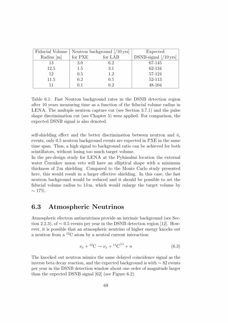
Fiducial Volume Neutron background [/10 yrs] ExpectedRadius [m] for PXE for LAB DSNB-signal [/10 yrs]

13 3.0 6.2 67-14512.5 1.5 3.1 62-13412 0.5 1.2 57-124

11.5 0.2 0.5 52-11311 0.1 0.2 48-104

Table 6.1: Fast Neutron background rates in the DSNB detection regionafter 10 years measuring time as a function of the fiducial volume radius inLENA. The multiple neutron capture cut (see Section 3.7.1) and the pulseshape discrimination cut (see Chapter 5) were applied. For comparison, theexpected DSNB signal is also denoted.

self-shielding effect and the better discrimination between neutron and νeevents, only 0.5 neutron background events are expected in PXE in the sametime span. Thus, a high signal to background ratio can be achieved for bothscintillators, without losing too much target volume.

In the pre-design study for LENA at the Pyhasalmi location the externalwater Cerenkov muon veto will have an elliptical shape with a minimumthickness of 2 m shielding. Compared to the Monte Carlo study presentedhere, this would result in a larger effective shielding. In this case, the fastneutron background would be reduced and it should be possible to set thefiducial volume radius to 13 m, which would enlarge the target volume by∼ 17%.

6.3 Atmospheric Neutrinos

Atmospheric electron antineutrinos provide an intrinsic background (see Sec-tion 2.2.3), of ∼ 0.5 events per year in the DSNB detection region [12]. How-ever, it is possible that an atmospheric neutrino of higher energy knocks outa neutron from a 12C atom by a neutral current interaction:

νx + 12C→ νx + 11C(∗)

+ n (6.3)

The knocked out neutron mimics the same delayed coincidence signal as theinverse beta decay reaction, and the expected background is with ∼ 82 eventsper year in the DSNB detection window about one order of magnitude largerthan the expected DSNB signal [62] (see Figure 6.2).

69

Figure 6.1: Fast Neutron background rates in the DSNB detection regionafter 10 years measuring time as a function of the fiducial volume radius inLENA for PXE (plotted in black) and LAB (plotted in red). The multipleneutron capture cut (see Section 3.7.1) and the pulse shape discriminationcut (see Chapter 5) were applied. Due to the higher discrimination efficiencyand self-shielding effect, the fast neutron background rate is less in PXE thanin LAB.

Figure 6.2: The expected atmospheric neutral current neutrino backgroundin LENA (plotted in red) after 10 years measuring time [62]. For comparison,the expected DSNB-signal according to the KRJ-model [32] is shown (plottedin blue).

70

Figure 6.3: Occupation of the 11C energy levels in the the simple shellmodel, with one hole in the S1/2 shell [63]. The energy difference betweenthe P3/2 and the S1/2 state is larger than separation energy for nucleons.Thus, the 11C will deexcitate mainly by the emission of protons, neutrons,or α−particles [63].

A first approach to reduce this background is to search for the decay of theproduced 11C atom.

However, the 11C isotope is produced in the ground state only two thirds ofthe time, in case that one of the four neutrons of the P3/2 shell is knockedout by the atmospheric neutrino [63]. One third of the time, the knock-outneutron is one of the two neutrons of the S1/2 shell and the resulting 11C atomis in an excited state (see Figure 6.3). As the excitation energy of the 11C∗

atom exceeds with ∼ 23 MeV the separation energy of nucleons in 11C, thenucleus will mainly deexcitate via the emission of protons, neutrons, or evenα−particles [63]. The deexciation by neutron emission happens 15% of thetime and can be identified by the additional 2.2 MeV signal from the neutroncapture on a proton. In the other case, the signal from the emitted protonsand α−particles can not be identified as is it superimposed with the promptsignal from the knocked out neutron. The residual daughter nucleii are eitherstable or have a halflife of ∼ 50 d or more. Thus, a direct identification ofthe deexcitation products is not possible.

The β+-decay of 11C has a half-life of 20 min and deposits between 1 MeVand 2 MeV in the scintillator. It should therefore be well above background,allowing to reject two thirds of the neutral current atmospheric events byvetoing on the coincidence with the initial neutron signal. If a neutron isknocked out of a 12C atom, the mean free distance between the reconstructed

71

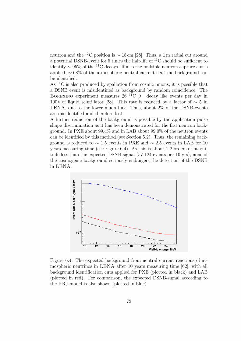
neutron and the 12C position is ∼ 18 cm [28]. Thus, a 1 m radial cut arounda potential DSNB-event for 5 times the half-life of 11C should be sufficient toidentify ∼ 95% of the 11C decays. If also the multiple neutron capture cut isapplied, ∼ 68% of the atmospheric neutral current neutrino background canbe identified.As 11C is also produced by spallation from cosmic muons, it is possible thata DSNB event is misidentified as background by random coincidence. TheBorexino experiment measures 26 11C β− decay like events per day in100 t of liquid scintillator [28]. This rate is reduced by a factor of ∼ 5 inLENA, due to the lower muon flux. Thus, about 2% of the DSNB-eventsare misidentified and therefore lost.A further reduction of the background is possible by the application pulseshape discrimination as it has been demonstrated for the fast neutron back-ground. In PXE about 99.4% and in LAB about 99.0% of the neutron eventscan be identified by this method (see Section 5.2). Thus, the remaining back-ground is reduced to ∼ 1.5 events in PXE and ∼ 2.5 events in LAB for 10years measuring time (see Figure 6.4). As this is about 1-2 orders of magni-tude less than the expected DSNB-signal (57-124 events per 10 yrs), none ofthe cosmogenic background seriously endangers the detection of the DSNBin LENA.

Figure 6.4: The expected background from neutral current reactions of at-mospheric neutrinos in LENA after 10 years measuring time [62], with allbackground identification cuts applied for PXE (plotted in black) and LAB(plotted in red). For comparison, the expected DSNB-signal according tothe KRJ-model is also shown (plotted in blue).

72

Chapter 7

Conclusions and Outlook

The proposed LENA detector has a great potential for the detection of rareνe events like the diffuse supernova neutrino background (DSNB). Presentday Water Cerenkov detectors like Super-Kamiokande are only able to setupper limits on the DSNB flux. Due to its large target mass of about 50 ktand the superior background discrimination of a liquid-scintillator detector,about 60-130 DSNB events will be identified in LENA after 10 years measur-ing time. As this rate is still low, background is a crucial issue for the DSNBdetection, even in a liquid-scintillator detector. Reactor νe and atmosphericνe provide an indistinguishable background and limit the detection regionto about 10 MeV to 25 MeV, exact upper and lower limit depending on thedetector site. Another important background source are fast neutrons thatare produced by cosmic muons in the surrounding rock and that propagateinto the detector, where they cause the same delayed coincidence signal asνe events.

In the present work, a GEANT4-based Monte Carlo simulation of this back-ground was performed. In a first step the neutron production in the rockwas simulated. At a depth of 4 km w.e. shielding, a muon that passes therock next to the detector produces on average ∼ 12 neutrons for 100 m tracklength. Out of them, 2.9 feature energies of 40 MeV or higher, which was de-termined by simulations to be the minimum required for reaching the targetvolume. These rates are in good agreement with similar simulations basedon the FLUKA code [45]. The simulated initial energy spectrum and angu-lar distribution were used as input values for the simulation of the neutronpropagation into the detector.

For both investigated scintillators, PXE and LAB, the fast neutron back-ground rate in the geoneutrino detection window was below 10 events peryear and is therefore insignificant compared to the ∼ 1000 expected geoneu-trino events.

73

In the DSNB detection window, about 70 fast neutron events per year areexpected in PXE and about 80 per year in LAB. This background can bereduced by a fiducial volume cut. In order to achieve a signal backgroundratio of about 10:1, a minimum shielding of about 7 m w.e. is needed. In thepresent setup of LENA this would reduce the target volume by about 40%.One method to suppress this background is to exclude events with morethan one neutron capture signal within 1 ms, as fast neutrons can generatesecondary neutrons, contrary to νe events. With this method, about 30%to 40% of the fast neutron events in the DSNB detection window can beidentified.As proton recoils of neutrons feature a different pulse shape than positronsgenerated in the inverse beta decay reaction, it is possible to identify neutronevents by pulse shape analysis. To obtain the necessary input parameters ofthe signal shapes, a laboraty experiment using a small scintillator cell and aAm-Be neutron source was performed. Neutron-induced proton- and gamma-induced electron recoils in the cell were analyzed. For PXE (with 10g

lPPO),

over 99.9% and for LAB (with 10gl

PPO) over 99% of the neutron eventswith an visible energy between 2 MeV and 3.5 MeV could be identified, if97.8% of the gamma events were accepted.Based on the experimental values, the efficiency of the pulse shape discrim-ination between neuton and νe events at visible energies between 10 MeVand 25 MeV was analyzed by a Monte Carlo simulation of LENA. In PXEover 99.4% and in LAB over 99.0% of the neutron events could be identified,while still accepting 95% of the νe events. As the pulse shape discriminationwas measured at low energies, the probability density functions (PDF) ofthe scintillation process for the positron and the recoil protons had to beextrapolated to the DSNB detection window.In order to reduce the systematic uncertainties that are generated by thisextrapolation, a measurement of the neutron pulse shape at energies above10 MeV should be performed. The laboratory experiment should be repeatedwith smaller PPO concentrations in the samples. The aspired PPO con-centration is about 2 g

lto avoid self-absorption processes of the wavelength

shifter [15].Applying all background suppression cuts and setting the fiducial volumeradius to 12 m, the expected fast neutron background rate for the DSNBdetection in LENA is about 0.5 fast neutron events in 10 years for PXE andabout 1.2 for LAB. As only 95% of the νe events are accepted due to thepulse shape discrimination, the expected DSNB signal is slightly reduced to57-124 events per 10 years.Two further cosmogenic background sourced were investigated. 9Li that isproduced in the liquid scintillator by cosmic muon spallations features a βn

74

decay that mimics the νe signals. If a cylinder of 2 m radius around eachcrossing muon is vetoed for 1 s, the background rate to the DSNB can bereduced to 0.7-0.8 events per 10 years measuring time.Another background is caused by atmospheric neutrinos that knock out neu-trons from 12C atoms by neutral current reactions. As about 820 events in10 years are expected, it is crucial for the DSNB detection to reduce thisbackground. One way to do this, is to search for the β− decay of 11C in itsground state, which is produced two thirds of the time, and for additionalneutrons from excited 11C, which are emitted 5% of the time. Due to randomcoincidences, this will cause a small reduction of the expected DSNB signalto 56-121 events per 10 years. As all other decay channels of 11C∗ can not bevetoed by coincidence with a delayed particle, the pulse shape discriminationhas to be used to reduce the background further to about 1.5 events for PXEand to about 2.5 for LAB per 10 years measuring time.It is evident that the cosmogenic background exceed the expected DSNBsignal without any background suppression cuts. While the fast neutronbackground can be reduced with an increase of the water shielding aroundthe buffer or a decrease of the fiducial volume radius to 10 m, the only wayto reduce the background from neutral current reactions of atmospheric neu-trinos is to perform the pulse shape discrimination of neutron and νe events.Experimental results at low visible energies between 2 MeV and 3.5 MeV in asmall scintillator cell and the simulation of the neutron-positron pulse shapediscrimination in the DSNB detection region in LENA demonstrated thegreat potential of this method. Based on the results of the present work, adetection of the DSNB with a signal to background ratio of about 10:1 orbetter is achievable with both PXE and LAB in LENA.

75

76

List of Figures

1.1 The MSW effect in the Sun . . . . . . . . . . . . . . . . . . . 5

1.2 The survival probability of νe from the Sun . . . . . . . . . . . 6

1.3 The Cerenkov effect . . . . . . . . . . . . . . . . . . . . . . . . 7

1.4 Schematical view of the Borexino detector . . . . . . . . . . 11

2.1 Schematical view of the LENA detector . . . . . . . . . . . . 14

2.2 The pp-chain . . . . . . . . . . . . . . . . . . . . . . . . . . . 17

2.3 The CNO-I-cycle and CNO-II-cycle . . . . . . . . . . . . . . . 17

2.4 Solar neutrino spectrum . . . . . . . . . . . . . . . . . . . . . 18

2.5 Reactor νe spectra at Frejus, Pyhasalmi and Hawaii . . . . . . 22

2.6 Expected DSNB signal in LENA . . . . . . . . . . . . . . . . 23

2.7 Predicted geoneutrino spectrum . . . . . . . . . . . . . . . . . 24

2.8 Expected signal of DM annihilation neutrinos in LENA . . . 26

3.1 Depth dependent mean muon energy . . . . . . . . . . . . . . 28

3.2 Feynman diagram of a muon spallation process . . . . . . . . 28

3.3 Simulated detector geometry . . . . . . . . . . . . . . . . . . . 30

3.4 Average neutron production along a muon path . . . . . . . . 33

3.5 Neutron production yield . . . . . . . . . . . . . . . . . . . . . 34

3.6 Fast neutron energy spectrum . . . . . . . . . . . . . . . . . . 35

3.7 Fast neutron multiplicity . . . . . . . . . . . . . . . . . . . . . 36

3.8 Fast neutron angular distribution . . . . . . . . . . . . . . . . 37

3.9 Schematic cross section through the simulated LENA detector 38

3.10 Simulated range of fast neutrons in LENA . . . . . . . . . . . 39

3.11 Initial energy spectrum of fast neutrons that reached the tar-get volume of LENA . . . . . . . . . . . . . . . . . . . . . . . 40

3.12 Total energy deposit of fast neutrons in LENA . . . . . . . . 41

3.13 Simulated photon signal of a neutron event, where a secondaryneutron was generated . . . . . . . . . . . . . . . . . . . . . . 44

3.14 Typical pulse shapes for α-particles, protons and electrons inliquid scintillator . . . . . . . . . . . . . . . . . . . . . . . . . 46

77

4.1 Schematic experimental setup . . . . . . . . . . . . . . . . . . 484.2 Neutron energy spectrum of a Am-Be source . . . . . . . . . . 494.3 Recorded pulse with subtracted baseline . . . . . . . . . . . . 504.4 Calibration of the experimental setup . . . . . . . . . . . . . . 514.5 Measured tail-to-total ratios in PXE . . . . . . . . . . . . . . 524.6 Energy dependence of the peak distance parameter D between

gamma and neutron peak in PXE and LAB . . . . . . . . . . 534.7 Energy dependence of the neutron tail-to-total ratio in PXE . 564.8 Simulated energy dependence of the peak distance parameter

D between gamma and neutron peak in PXE . . . . . . . . . . 574.9 Simulated energy dependence of the peak distance parameter

D between gamma and neutron peak in LAB . . . . . . . . . . 57

5.1 Comparison of the average pulse shape with and without timeof flight correction in LENA . . . . . . . . . . . . . . . . . . . 61

5.2 Tail-to-total ratio of positrons and neutrons in PXE . . . . . . 625.3 Energy dependent neutron rejection efficiency in LENA . . . 635.4 Average pulse shape of 10 MeV positrons in PXE with 20 m

scattering length and a hypothetical scattering length of 20 km 65

6.1 Fast Neutron background rates in the DSNB detection regionin LENA . . . . . . . . . . . . . . . . . . . . . . . . . . . . . 70

6.2 Expected atmospheric neutral current neutrino background inLENA . . . . . . . . . . . . . . . . . . . . . . . . . . . . . . . 70

6.3 Occupation of the 11C energy levels in the the simple shellmodel with one hole in the S1/2 shell . . . . . . . . . . . . . . 71

6.4 Expected background from neutral current reactions of atmo-spheric neutrinos in LENA with all background identificationcuts applied . . . . . . . . . . . . . . . . . . . . . . . . . . . . 72

78

List of Tables

1.1 Leptons in the scope of the weak interaction . . . . . . . . . . 21.2 Neutrino square mass differences and mixing angles . . . . . . 4

2.1 Solar neutrino event rates in LENA . . . . . . . . . . . . . . 192.2 Expected event rates in LENA for a supernova explosion in

the center of our galaxy . . . . . . . . . . . . . . . . . . . . . 20

3.1 Relative contribution of individual processes to the total neu-tron production yield . . . . . . . . . . . . . . . . . . . . . . . 36

3.2 Fast neutron background rates per year in LENA for PXE . . 423.3 Fast neutron background rates per year in LENA for LAB . . 423.4 Fast neutron background rates per year in LENA for PXE

after the application of a multiple neutron capture veto . . . . 453.5 Fast neutron background rates per year in LENA for LAB

after the application of a multiple neutron capture veto . . . . 45

4.1 Energy dependence of the neutron rejection efficiency in PXEand LAB . . . . . . . . . . . . . . . . . . . . . . . . . . . . . . 53

5.1 Scintillation properties for LAB and PXE . . . . . . . . . . . 60

6.1 Fast Neutron background rates in the DSNB detection regionwith all background identification cuts applied . . . . . . . . . 69

79

80

Bibliography

[1] W. Pauli. Collected Scientific Papers, volume Vol. 2. Interscience, NewYork, 1964.

[2] D. Autiero et al. Large underground, liquid based detectors for astro-particle physics in Europe: scientific case and prospects. JCAP,0711:011, 2007.

[3] L. Bergstrom, A. Goobar. Cosmology and Particle Astrophysics, vol-ume 2. Springer, 2003.

[4] C. Amsler et al. (Particle Data Group). Physics Letters, B667:1, 2008.

[5] A. Djouadi. The Anatomy of Elctro-Weak Symmetry Breaking. I: TheHiggs boson in the Standard Model. Phys.Rept., 457:1–216, 2008.

[6] SNO Collaboration. Electron Energy Spectra, Fluxes, and Day-NightAsymmetries of 8B Solar Neutrinos from the 391-Day Salt Phase SNOData Set. Phys. Rev., C72:055502, 2005. hep-ex/0508053v2.

[7] Super-Kamiokande Collaboration. Solar neutrino measurements insuper-kamiokande-i. Phys. Rev., D73:112001, 2006. hep-ex/0508053v2.

[8] S.M. Bilenky, C. Giunti, W. Grimus. Phenomenology of Neutrino Os-cillations. Prog.Part.Nucl.Phys., 43:1–86, 1999. hep-ph/9812360v4.

[9] N. Schmitz. Neutrinophysik. Teubner Studienbucher, Stuttgart, 1997.

[10] M. Apollonio et al. Search for neutrino oscillations on a long base-lineat the chooz nuclear power station. Eur.Phys.J., C27:331–374, 2003.hep-ex/0301017v1.

[11] B. T. Cleveland et al. Astrophys. J., 496:505, 1998.

[12] M. Wurm. Cosmic Background Discrimination for the Rare NeutrinoEvent Search in Borexino and LENA. PhD thesis, Technische Univer-sitat Munchen, 2009.

81

[13] J. D. Jackson. Classical Electrodynamics. Wiley, New York, 1962.

[14] Y. Takeuchi. Measurement of Solar Neutrinos from One Thousand Daysof Data at Kamiokande-III. PhD thesis, Tokyo Inst. of Tech., 1995.

[15] T. Marrodan Undagoitia. Measurement of light emission in organicliquid scintillators and studies towards the search for proton decay inthe future large-scale detector LENA. PhD thesis, Technische UniversitatMunchen, 2008.

[16] Borexino Collaboration. Pulse Shape discrimination with the CountingTest Facility. Nucl.Instrum.Meth., A584:98–113, 2007. 0805.3843v2.

[17] J. G. Learned. High energy neutrino physics with liquid scintillationdetectors, 2009. 0902.4009v1.

[18] M. Wurm et al. Detection potential for the diffuse supernova neutrinobackground in the large liquid-scintillator detector lena. Phys. Rev. D75,023007, 2007. astro-ph/0701305v1.

[19] M. Pallavicini. Getting the first 7Be ν detection: scintillator purification,detector response and data analysis in Borexino. In TAUP, 2007.

[20] Borexino Collaboration. First real time detection of 7Be solar neutrinosby Borexino. Phys.Lett., B658:101–108, 2007. 0708.2251v2.

[21] Borexino Collaboration. New results on solar neutrino fluxes from 192days of borexino data. Phys. Rev. Lett., 101:091302, 2008. 0805.3843v2.

[22] Kalliossuunnittelu Oy Rockplan LTD. www.rockplan.fi/, 2008.

[23] D. Autiero et al. Large underground, liquid based detectors for astro-particle physics in europe: scientific case and prospects. JCAP 0711:011,2007. arXiv:0705.0116v2.

[24] J.N. Bahcall. Solar Neutrinos. Encyclopedia of Physics, 3rd edition, Vol.2:2242, 2005.

[25] E. Adelberger et al. Solar Fusion Cross Sections. Rev.Mod.Phys.,70:1265–1292, 1998. astro-ph/9805121.

[26] J.N. Bahcall, A.M. Serenelli, S. Basu. New solar opacities, abundances,helioseismology, and neutrino fluxes. Nucl. Instrum. Meth., A505:688–698, 2003. hep-ex/0303007.

82

[27] S. Todor. Solar Neutrinos with LENA and a spectroscopical analysisof liquid scintillators. Diploma thesis, Technische Universitat Munchen,2008.

[28] Q. Meindl. Indentification of Cosmogenic Background Signals in theNeutrino Experiment Borexino. Diploma thesis, Technische UniversitatMunchen, 2008.

[29] J. Winter. Phenomenology of Supernova Neutrinos, Spatial Event Re-construction, and Scintillation Light Yield Measurements for the Liquid-Scintillator Detector LENA. Diploma thesis, Technische UniversitatMunchen, 2007.

[30] K. Kotake, K. Sato, K. Takahashi. Explosion mechanism, neu-trino burst, and gravitational wave in core-collapse supernovae.Rept.Prog.Phys., 69:971–1144, 2006. astro-ph/0509456.

[31] Super-Kamiokande Collaboration, M. Malek et al. Search for supernovarelic neutrinos at super-kamiokande. Phys.Rev.Lett., 90:061101, 2003.hep-ex/02090282v2.

[32] M. T. Keil, G. G. Raffelt, H. T. Janka. Monte carlo study of supernovaneutrino spectra formation. Astrophys.J., 590:971–991, 2003. astro-ph/0208035v2.

[33] T. Totani et al. Future detection of supernova neutrino burst and explo-sion mechanism. Astrophys.J., 496:216–225, 1998. astro-ph/9710203v1.

[34] T. A. Thompson, A. Burrows, P. A. Pinto. Shock breakout in core-collapse supernovae and its neutrino signature. Astrophys.J., 592:434,2003. astro-ph/0211194.

[35] K. A. Hochmuth. Low Energy Neutrinos as geological and astrophysicalMessengers. PhD thesis, Technische Universitat Munchen, 2008.

[36] W.F. McDonough and S.S. Sun. The composition of the Earth. Chem.Geol., 120:223, 1995.

[37] K.A. Hochmuth et al. Probing the earth’s interior with a large-volumeliquid scintillator detector. Astropart.Phys., 27:21–29, 2007. hep-ph/0509136v3.

[38] T. Araki et al. Nature, 436:499, 2005.

83

[39] P. Nath, P. F. Perez. Proton stability in grand unified theories, in strings,and in branes. Phys.Rept., 441:191–317, 2007. hep-ph/0601023v3.

[40] Super-Kamiokande Collaboration,H. Nishino,S. Clark et a. Search forproton decay via p → e+π0 and p → µ+π0 in a large water cherenkovdetector. Phys.Rev.Lett., 102:141801, 2009. hep-ex/0903.0676v2.

[41] Super-Kamiokande Collaboration. Search for nucleon decay viamodes favored by supersymmetric grand unification models in super-kamiokande-i. Phys.Rev., D72:052007, 2005. hep-ex/0502026v1.

[42] S. Palomares-Ruiz, S. Pascoli. Testing mev dark matter with neutrinodetectors. Phys.Rev., D77:025025, 2008. 0710.5420v1.

[43] G. Bertone, D. Hopper, J. Silk. Particle dark matter: Evidence,candidates and constraints. Phys.Rept., 405:279–390, 2005. hep-ph/0404175v2.

[44] C. Boehm, P. Fayet, J. Silk. Light and heavy dark matter particles.Phys.Rev., D69:101302, 2004. hep-ph/0311143v1.

[45] V. A. Kudryavtsev, N. J. C. Spooner, J. E. McMillan. Simulations ofmuon-induced neutron flux at large depths underground. Astrophys.J.,621:L85, 2005. arXiv:astro-ph/0303007v1v3.

[46] Y-F. Wang et al. Predicting Neutron Production from Cosmic-rayMuons. Phys.Rev. D, 64:013012, 2001. hep-ex/0101049v1.

[47] S. Agostinelli et al. Geant4 - a simulation toolkit. Nuclear Instrumentsand Methods, 1A 506:250–303, 2003.

[48] Geant4 Colloboration. Geant4: Physics reference manual, 2009.http://geant4.web.cern.ch/geant4/UserDocumentation/UsersGuides/PhysicsReferenceManual/fo/PhysicsReferenceManual.pdf.

[49] Geant4 Colloboration. Geant4: Testing and validation, 2009.http://geant4.web.cern.ch/geant4/results/results.shtml.

[50] J. Apostolakis et al. Progress in hadronic physics modelling in geant4.Journal of Phys.: Conference Series, 160:012073, 2009.

[51] J. B. Birks. The Theory and Practise of Scintillation Counting.Pergamon-Press, London, 1964.

[52] R. Brun, F. Rademakers, 1998. http://root.cern.ch.

84

[53] LVD Collaboration. Measurement of the Neutron Flux Produced byCosmic-Ray Muons with LVD at Gran Sasso. In Proc. of 26th Intern.Cosmic Ray Conf., Salt Lake City, USA, 1999. hep-ex/9905047.

[54] C.M. Lederer and V.S. Shirley (Ed.). Table of Isotopes, seventh edition.John Wiley and Sons, 1978.

[55] T. Jagemann. Measurement of the Scintillation Light Quenching forNuclear Recoils induced by Neutron Scattering in Detectors for DarkMatter Particles. PhD thesis, Technische Universitat Munchen, 2004.

[56] C. Ciemniak. PhD thesis, Technische Universitat Munchen, in prepara-tion.

[57] M.J. Berger, J.S. Coursey, M.A. Zucker and J. Chang. ESTAR, PSTAR,and ASTAR: Computer Programs for Calculating Stopping-Power andRange Tables for Electrons, Protons, and Helium Ions (version 1.2.3),2005. [Online] Available: http://physics.nist.gov/Star [2009, October30]. National Institute of Standards and Technology, Gaithersburg, MD.

[58] H.O. Back et al. Phys. Lett., B 525:205, 2002.

[59] KamLAND Collaboration. A High Sensitivity Search for νe’s from theSun and Other Sources at KamLAND. Phys.Rev.Lett., 92:071301, 2004.

[60] T. Hagner et al. Astropart. Phys., 14:33, 2000.

[61] A. Tang, G. Horton-Smith, V.A. Kudryatsev, A. Tonazzo. Muon Sim-ulations for Super-Kamiokande, KamLAND and CHOOZ. Phys.Rev.D,74:053007, 2006. hep-ph/0604078v2.

[62] Y. Efremenko. Signatures of Nucleon Disappearance in Large Under-ground Detectors. In Advances in Neutrino Technology, August 2009.

[63] Y. Kamyshkov, E. Kolbe. Signatures of Nucleon Disappearance inLarge Underground Detectors. Phys.Rev. D, 67:076007, 2003. nucl-th/0206030v2.

85

86

Danksagung

An erster Stelle mochte ich bei Prof. Franz von Feilitzsch fur die freundlicheAufnahme an seinem Lehrstuhl E15 und viele interessante Diskussionen, auchuber nicht-physikalische Themen, bedanken.Desweiteren will ich bei Prof. Lothar Oberauer fur das Stellen eines inter-essanten Diplomarbeitsthemas und dafur das er immer ein offenes Ohr furFragen hatte bedanken.Daruberhinaus will ich bei Michael Wurm fur die hervorragende Betreuungund das Korrekturlesen dieser Arbeit bedanken.Entscheidenden Anteil an dieser Arbeit hatte Raimund Strauss, mit dem ichdie Messung der Neutron-Gamma Pulsform Discrimination durchfuhrte undohne dessen Hilfe meine Diplomarbeit in dieser Form nicht moglich gewesenware.Ebenso will ich bei Teresa Marrodan Undagoitia und Jurgen Winter be-danken. Ihre LENA-Simulation bildete die Grundlage fur diese Arbeit.Ein großer Dank gilt meinen Burokollegen: Martin Hofmann, Achim Gutleinund Nils Haag, die mir einerseits jederzeit bei kleineren oder großeren Pro-blemen geholfen haben und andererseits fur eine sehr angenehme Arbeitsat-mosphare gesorgt haben. Besonders mochte ich mich noch einmal bei MartinHofmann fur das Korrekturlesen dieser Arbeit bedanken.Fur die Einfuhrung in den Arbeitsalltag eines Borexino-Shifters (”dieseFehlermeldungen kannst du ignorieren....die ebenso”) mochte ich bei QuirinMeindl bedanken.Bei Maria Bremberger mochte ich mich fur die bereitwillige Hilfe beim Aus-fullen diverser Formulare bedanken.Ein großer Dank gilt allen anderen Mitgliedern des E15 Lehrstuhls, die ichhier nicht namentlich genannt habe, die stets hilfsbereit waren und fur eineangenehme Atmosphare gesorgt haben.Bei meiner Schwester mochte ich mich dafur bedanken, das sie dieses Werkklaglos nach sprachlichen Fehlern durchsucht hat.Zuletzt mochte ich noch bei Eltern dafur bedanken, das sie mir dieses Studiumermoglicht haben, und mich jederzeit dabei unterstutzt haben.

87