Analysis of randomly stacked pebble bed reactors using

a Monte Carlo neutron transport code with a statistical

geometry model

PNR-131-2011-005

Günther Ouwendijk

May 2011

Delft University of Technology

Faculty of Applied Sciences

Department of Radiation, Radionuclides & Reactors

Section Physics of Nuclear Reactors

Analysis of randomly stacked pebble bed reactors using a Monte Carlo neutron transport code with a statistical

geometry model

Günther Ouwendijk

Supervisors:

Gert-Jan Auwerda, MSc

dr.ir. Jan-Leen Kloosterman

Delft, May 2011

i

Abstract

In order to be able to calculate the neutronics of a nuclear reactor with a Monte Carlo

code, it is necessary to know the exact geometry of the reactor. However, for a pebble

bed reactor the exact location of the fuel is unknown because not only are the TRISO

particles randomly distributed inside the pebbles, but also the pebbles themselves are

randomly stacked inside the reactor. A way around this problem is to use a statistical

geometry model in which probability density functions are used to calculate the distance

that a neutron travels in the void space between the pebbles when it exits a pebble, and

what the orientation of the next pebble is with respect to its flight path.

In this research project the accuracy of a statistical geometry model for the

analyses of a randomly stacked pebble bed reactor was examined, by comparing the

results from a Monte Carlo code in which a statistical geometry model is incorporated

with those of a regular Monte Carlo code. Three different boundary conditions were

investigated: no partial pebbles at the boundary, partial pebbles at the boundary, and

partial pebbles at the boundary with the additional requirement that the center of each

pebble still has to be inside the reactor. The influence of the absorption cross-section

and the packing density fluctuations near the boundary of the reactor as well as the

effect of using different probability density functions for two extra zones near the

boundary on the accuracy of the statistical geometry model was also investigated.

Two basic Monte Carlo codes were written. MC-Fixed uses a pre-generated

pebble bed for its calculations, and was also used to calculate the probability density

functions for the statistical geometry model. MC-SGM uses a statistical geometry model

for its calculations.

Using a statistical geometry model for the analyses of a randomly stacked pebble

bed reactor resulted in a 3% overestimation of keff for a very small reactor and a 0.1%

overestimation of keff for a large reactor. If no partial pebbles are allowed at the boundary,

the pebble density near the boundary is underestimated resulting in an underestimation

of keff. If partial pebbles are allowed at the boundary, the results are excellent for a large

reactor, but for a small reactor the pebble density near the boundary is overestimated

resulting in an overestimation of keff. If the center of each pebble has to be inside the

reactor, the results for a small reactor improve significantly, while for a large reactor the

results improve slightly. However, for a very small reactor, the pebble density near the

boundary is still slightly overestimated resulting in a small overestimation of keff.

The absorption cross-section has no discernable influence on the accuracy of the

statistical geometry model. The fluctuations in packing density near the boundary locally

influence the probability density function for the distance that a neutron travels in the

void space between the pebbles. However, only for a small reactor there is a significant

influence of the packing density fluctuations on the accuracy of the statistical geometry

model, therefore, the use of different probability density functions for extra two zones

close to the boundary only improves the accuracy for a small reactor, and has no

significant effect on the accuracy of the statistical geometry model for a large reactor.

ii

iii

Contents

ABSTRACT .......................................................................................................................................I

CONTENTS .....................................................................................................................................III

INTRODUCTION ..............................................................................................................................1

1.1 WHY NUCLEAR ENERGY? ...........................................................................................................1 1.2 THE PEBBLE BED REACTOR ........................................................................................................1 1.3 ANALYSIS OF A RANDOMLY STACKED PEBBLE BED REACTOR ........................................................3 1.4 THESIS OUTLINE .......................................................................................................................4

THEORETICAL BACKGROUND .....................................................................................................7

2.1 NUCLEAR REACTOR PHYSICS .....................................................................................................7 2.1.1 Nuclear fission ................................................................................................................7 2.1.2 The criticality of a nuclear reactor ...................................................................................8 2.1.3 Neutron cross-sections ...................................................................................................9 2.1.4 The integral neutron transport equation..........................................................................9

2.2 MONTE CARLO SIMULATION .................................................................................................... 11 2.2.1 The Monte Carlo method ............................................................................................. 11 2.2.2 Solving the transport equation using Monte Carlo ....................................................... 12 2.2.3 Simulating a neutron flight path ................................................................................... 13 2.2.4 Estimators .................................................................................................................... 14 2.2.5 Variance & variance reduction ..................................................................................... 15

2.3 THE STATISTICAL GEOMETRY MODEL ....................................................................................... 17

THE MONTE CARLO CODES ...................................................................................................... 21

3.1 THE MONTE CARLO CODE MC-FIXED ...................................................................................... 21 3.1.1 General overview of the Monte Carlo code ................................................................. 21 3.1.2 The simulation of a neutron flight path ......................................................................... 22 3.1.3 Validation of MC-Fixed ................................................................................................. 25

3.2 THE MONTE CARLO CODE MC-SGM ...................................................................................... 26

RESULTS ...................................................................................................................................... 29

4.1 THE PROBABILITY DENSITY FUNCTIONS ................................................................................. 29 4.1.1 The entrance angle distribution ................................................................................... 30 4.1.2 The distribution of the distance that neutrons travel in the void space ........................ 30

4.2 ORDERED PEBBLE BED STACKINGS ......................................................................................... 31 4.2.1 Testing for convergence of the fission source in MC-SGM ......................................... 31 4.2.2 The criticality calculations ............................................................................................ 33 4.2.3 Recalculation of the criticality with MC-SGM ............................................................... 36 4.2.4 Conclusions ................................................................................................................. 39

4.3 RANDOMLY STACKED PEBBLE BEDS......................................................................................... 39 4.3.1 The criticality calculations ............................................................................................ 39 4.3.2 Recalculation of keff with a different boundary condition for MC-SGM ........................ 41 4.3.3 Testing a third boundary condition for MC-SGM ......................................................... 42 4.3.4 Conclusions ................................................................................................................. 43

4.4 THE INFLUENCE OF THE ABSORPTION CROSS-SECTION ............................................................. 44 4.5 THE INFLUENCE OF PACKING DENSITY FLUCTUATIONS NEAR THE WALL ...................................... 45

4.5.1 The influence of the packing density fluctuations on the results ................................. 45 4.5.2 The influence of packing density fluctuations on the local distance that the neutrons travels in the void space .............................................................................................. 48 4.5.3 Using different cdf’s for different zones in the pebble bed........................................... 49

iv

4.5.4 Conclusion ................................................................................................................... 51

CONCLUSIONS AND RECOMMENDATIONS ............................................................................ 53

5.1 CONCLUSIONS ....................................................................................................................... 53 5.2 RECOMMENDATIONS .............................................................................................................. 54

ACKNOWLEDGEMENTS ............................................................................................................. 55

BIBLIOGRAPHY ........................................................................................................................... 57

1

Chapter 1

Introduction

1.1 Why nuclear energy?

The increase of the global population in combination with industrial development will

lead to an expected doubling of the electricity consumption by the year 2030 [1]. At the

same time there are increasing global concerns about the effects of global warming and

climate change and the costs of fossil fuels continue to increase while their supplies

decline. There is therefore a need for a reliable energy source with low carbon dioxide

emissions such as nuclear energy to reduce and replace the use of fossil fuels. Together

with the improved economics of nuclear reactors caused by the increasing costs of fossil

fuels, this has lead to a renewed global interest in nuclear energy.

Although nuclear reactors are a possible solution for the need for a reliable and

low emission energy source, there are also concerns about the safety of nuclear reactors

and the resulting nuclear waste. This has lead to the need for a new generation of

advanced nuclear reactors with increased safety features and minimum nuclear waste.

There are currently several designs being investigated for future development which are

gathered under the name generation IV nuclear reactors [2]. One of these designs is the

pebble bed reactor.

1.2 The pebble bed reactor

The pebble bed reactor is a gas cooled, graphite moderated reactor that consists

of a large cylindrical pressure vessel which is lined with a graphite reflector, and contains

up to half a million randomly stacked spherical fuel elements [3]. The spherical fuel

elements, called pebbles, can be extracted from the bottom of the reactor vessel and

refilled at the top which makes online refueling possible. The reactor is cooled by helium

that flows through the graphite reflector and the void spaces between the pebbles.

2

The pebbles are graphite spheres with a diameter of approximately 60 mm that

contain thousands of TRISO fuel particles which are randomly distributed throughout the

fuel zone of the pebble. The TRISO particles have a diameter of approximately 1 mm

and consist of a fuel kernel made of UO2 that is covered with several layers of silicon

carbide and pyrolytic carbon. The graphite of the fuel pebbles also acts as a moderator.

Figure 1.1: Schematic overview of a pebble bed reactor [4].

Figure 1.2: Schematic overview of the pebbles and TRSISO particles [3].

3

One of the major advantages of the design of a pebble bed reactor is that it can

be designed to be inherently safe [3,5]. The pebble bed reactor has a low power density

which means that the amount of energy and heat produced per unit volume is low. This

makes it possible for the heat to be removed from the core by natural mechanisms alone

such as conductive and radiative heat transfer in case of an incident such as the loss of

cooling. This means that during an accident the temperature inside the reactor can never

become high enough to damage the pebbles or the TRISO particles. A second safety

aspect of the design of the pebble bed reactor is the use of TRISO particles. The layers

of silicon carbide and pyrolytic carbon that cover the fuel kernel retain the fission

products that are created inside the fuel kernel. This means that the coolant does not get

contaminated and that there is no significant radiation released in case of an accident.

Another advantage of the design of a pebble bed reactor is the possibility of a

high outlet temperature of the helium flow which makes it possible to reach a thermal

efficiency as high as 50%, which is considerably higher than 35% achieved in traditional

reactor designs [6].

1.3 Analysis of a randomly stacked pebble bed reactor

One of the main goals in nuclear reactor physics is to calculate the neutron distribution

and the behavior of the neutron population over time inside a nuclear reactor. The

neutron flux distribution for example determines the rate and distribution of the nuclear

reactions inside the reactor, and the behavior of the neutron population over time tells

something about the stability of the fission chain reaction.

The analyses of the neutronics of a nuclear reactor are often performed using a

Monte Carlo neutron transport code. The Monte Carlo method uses random numbers to

solve a physical problem by simulating a large number of events to gain insight into how

the system behaves [7]. In case of a neutronics calculation of a nuclear reactor this

means that a large number of neutron flight paths are simulated by sampling from the

appropriate probability density functions using random numbers. A detailed overview of

the Monte Carlo method is given in chapter 2.

Monte Carlo codes are capable of performing neutronics calculations for any

nuclear reactor geometry. However, in order to be able to calculate the neutronics of a

nuclear reactor it is necessary to know the exact geometry of the reactor, and in case of

a pebble bed reactor this means that it is necessary to know the exact location of each

TRISO particle and of every pebble of the pebble bed. Unfortunately, the exact locations

of both the pebbles and of the TRISO particles inside the pebbles are unknown because

not only are the TRISO particles randomly distributed inside the pebbles but also the

pebbles themselves are randomly stacked inside the reactor.

The usual solution to this problem is to model the core of the reactor as a

homogeneous mixture of the pebble material and helium [8]. In this way, it is no longer

necessary to know the exact location of all the pebbles and TRISO particles in order to

be able to perform a neutronics calculation of the reactor. Unfortunately, not all the

4

effects of the pebble bed on the neutronics are included in this model, which can result

in possible errors in the calculation. Another option is to first compute a randomly

stacked pebble bed, and perform the calculation on this pebble bed. However, a pebble

bed reactor can contain up to half a million pebbles, and generating such a large

randomly stacked pebble bed requires a considerable amount of computation time.

A way around these problems is to use a statistical geometry model in the Monte

Carlo code as described by Murata et al.[9,10] in which probability density functions are

used to calculate the distance that a neutron will travel in the void space between the

pebbles when it exits a pebble, and what the orientation of the next pebble is with

respect to its flight path. When a statistical geometry model is incorporated into a Monte

Carlo code it is therefore no longer necessary to know the exact location of the pebbles

in order to be able to perform a neutronics calculation of a randomly stacked pebble bed

reactor. A detailed description of the statistical geometry model is given in chapter 2.

However, there are still some of questions left about using a statistical geometry

model for calculating the neutronics of a pebble bed reactor. Because probability density

functions are used to describe the streaming of the neutrons through the void space

between the pebbles some information about the pebble bed is lost, which could result in

possible errors in the calculations. Another issue is that the probability density function

that is used to calculate the distance that a neutron will travel in the void space depends

on the packing density of the pebble bed. However, the packing density of the pebbles is

not the same everywhere in the reactor because of the influence the boundary of the

reactor has on the pebble bed [11].

1.4 Thesis outline

The research in this thesis was performed as a Master End Project (MEP) in the Physics

of Nuclear Reactors group (PNR) of the faculty of applied physics at the Delft University

of Technology. The main goal of this research project was to examine the accuracy of

the statistical geometry model, by comparing the results from a Monte Carlo code in

which a statistical geometry model is incorporated with those of a regular Monte Carlo

code. The influence of the absorption cross-section and the packing density fluctuations

near the boundary of the reactor as well as the effect of using different probability

density functions for two extra zones near the boundary of the reactor on the accuracy of

the statistical geometry model was also investigated.

Two basic Monte Caro codes were written. Both codes use only one energy

group and the only neutron interactions that were considered are isotropic scattering,

capture and fission. The first Monte Carlo code uses a pre-generated randomly stacked

pebble bed for its calculations, and was used to calculate the necessary probability

density functions for the statistical geometry model. The second Monte Carlo code uses

a statistical geometry model for its calculations.

5

This thesis starts with a brief introduction of the theory in chapter 2. The chapter

starts with an introduction of the basics of nuclear reactor physics. Then, the Monte

Carlo method is introduced and it is explained how it can be used to calculate the

neutronics of a nuclear reactor. The chapter ends with a more detailed description of the

statistical geometry model.

The third chapter in this thesis is used to give a detailed description of the two

Monte Carlo codes that were written during this research project. First, the Monte Carlo

code MC-Fixed is described which uses a pre-generated randomly stacked pebble bed

for its calculations. This Monte Carlo code has been validated and the results of the

validation are given in this chapter. The second part of the chapter is used to describe

the Monte Carlo code MC-SGM that uses a statistical geometry model for its calculations.

The results of this research are presented in chapter 4. First, the two probability

density functions for the statistical geometry model that were calculated with MC-Fixed

are presented. Then, as a first test for both the statistical geometry model and MC-SGM,

the criticality of several pebble bed reactors with an ordered pebble bed stacking was

calculated. To investigate the accuracy of the statistical geometry for the analyses of a

randomly stacked pebble bed reactor, the criticality of several randomly stacked pebble

bed reactors was calculated. Next, the influence of the absorption cross-section on the

accuracy of the statistical geometry model was investigated. Finally, the influence of the

packing density fluctuations in a randomly stacked pebble bed reactor on the accuracy

of the results was investigated as well as the possibility to use different probability

density functions for different zones in the pebble bed reactor to improve the accuracy of

the statistical geometry model.

Finally, in chapter 5 the conclusions of this research project are presented as well

as several recommendations for future work.

6

7

Chapter 2

Theoretical background

2.1 Nuclear reactor physics

2.1.1 Nuclear fission

The principle behind a nuclear reactor is that a neutron can cause the nucleus of certain

heavy nuclei to split into two smaller nuclei, releasing a large amount of energy and

several new neutrons [12]. The neutrons that are released during a fission reaction can

themselves induce another fission, thereby releasing more energy and neutrons,

causing a chain reaction. If on average one of the neutrons that are released during a

fission reaction induces a new fission, a steady chain reaction is created during which a

continuous amount of energy is released.

Figure 2.1: The fission reaction [13].

The mass of a nucleus is usually less than that of the sum of the individual

nucleons that make up the nucleus. This mass defect has been converted into potential

energy and is called the binding energy and is the result of the nuclear forces that hold

8

the nucleus together. The average binding energy per nucleon depends on the number

of nucleons inside the nucleus. In figure 2.2 the average binding energy per nucleon is

plotted as a function of the number of nucleons in the nucleus. The graph shows that the

average binding energy per nucleon first increases up to a maximum around 56Fe and

then decreases again. Therefore, energy is released during the fusion of two light nuclei

or by splitting a heavy nucleus into two smaller nuclei.

Figure 2.2: The binding energy per nucleon as a function of the number of nucleons in the nucleus [14].

2.1.2 The criticality of a nuclear reactor

The multiplication factor keff is the number of neutrons in one generation with respect to

the number of neutrons in the previous generation [12].

number of neutrons in generation 1

2.1number of neutrons in generation

eff

ik

i

When keff is smaller than 1 the reactor is subcritical, the neutron population inside the

reactor will decrease over time and the fission chain reaction will die out. When keff is

larger than 1 the reactor is supercritical, the number of neutrons inside the reactor will

increase over time and the chain reaction is therefore also unstable. Finally, when keff is

equal to 1 the reactor is critical, the neutron population in the reactor is stable and the

power output of the reactor is constant.

9

2.1.3 Neutron cross-sections

The probability of a particular type of interaction between an incident neutron and a

single target nucleus is given by the microscopic cross-section σ which depends on the

type of interaction, the type of nucleus involved, and the energy of the neutron [12].

2

number of reactions/nucleus/s 2.2

number of incident neutrons/cm /s

The microscopic cross-sections that belong to each type of interaction are called partial

cross-sections and can be added up, giving the total microscopic cross-section σt which

represents the probability that the incident neutron undergoes any type of interaction

with the target nucleus.

= + + 2.3t i s c f

i

Here the subscripts s, c, and f stand for respectively scatter, capture and fission of the

incident neutron. The macroscopic cross-section Σ is the probability that a neutron

undergoes an interaction with a nucleus per unit length traveled through a material and

is given by

2.4N

in which N is the atomic number density.

2.1.4 The integral neutron transport equation

The time independent neutron distribution in a reactor is described by the stationary

neutron transport equation [7].

0 4

, , , , , , ' , ' , ', ' ' ' 2.5

+ , ,

t sE E E E E E d dE

s E

Ω r Ω r r Ω r Ω Ω r Ω Ω

r Ω

in which φ(r,E,Ω) is the angular neutron flux at location r with energy E in direction Ω,

Σs(r,E’→E,Ω’→Ω) is the macroscopic differential scattering cross-section, Σt(r,E) is the

total macroscopic cross-section and s(r,E,Ω) is the neutron source density.

The neutron transport equation is an integro-differential equation, while the

Monte Carlo method is suitable for solving integral problems. It is therefore necessary to

10

first transform the neutron transport equation into an integral equation. This can be done

by integrating the equation, but an easier way is to look at the physical processes that

take place in neutron transport [7]. In order to do this it is necessary to first introduce two

new variables. The first variable is the collision density ψ(r,E,Ω) where

, , 2.6E d dEd r Ω r Ω

is the number of neutrons in drdEdΩ entering a collision. The collision density and the

angular neutron flux are related by

, , , , , 2.7tE E E r Ω r r Ω

The second variable that needs to be introduced is the emission density χ(r,E,Ω) where

, , 2.8E d dEd r Ω r Ω

is the number of neutrons that start a flight path in drdEdΩ.

The flight path of each neutron, as it moves through a nuclear reactor, can be

described as a series of collisions and the transport of the neutron between those

collisions. The transport of a neutron from one location to the location of its next collision

is described by the transport kernel T(r’→r,E,Ω), where

' , , 2.9T E dr r Ω r

is the probability that a neutron starting at r’ with energy E and direction Ω has its next

collision in a volume dr around r. The collisions of each neutron are described by the

collision kernel C(r,E’→E,Ω’→ Ω), where

, ' , ' 2.10C E E dEd r Ω Ω Ω

is the probability that a neutron entering a collision at r with energy E’ and direction Ω’ to

exit the collision with energy E in dE and a direction Ω in dΩ.

The collision density ψ(r,E,Ω) and the emission density χ(r,E,Ω) can now be

written in terms of the transport and collision kernels and the neutron source distribution:

, , ' , , ', , ' 2.11V

E T E E d r Ω r r Ω r Ω r

0 4

, , , , , ' , ' , ', ' ' ' 2.12E s E C E E E d dE

r Ω r Ω r Ω Ω r Ω Ω

11

Substituting Eq. (2.12) into Eq. (2.11) gives the integral equation for the collision density.

0 4

, , , , ', ' , ' ', ', ' ' ' ' 2.13V

E S E L E E E d dE d

r Ω r Ω r r Ω Ω r Ω Ω r

in which the first flight collision density Sψ is give by

, , ' , , ', , ' 2.14V

S E T E S E d r Ω r r Ω r Ω r

and the transport kernel L for the collision density is given by

', ' , ' ', ' , ' ' , , 2.15L E E C E E T E r r Ω Ω r Ω Ω r r Ω

In the same way it is possible to derive an integral equation for the emission density by substituting Eq. (2.11) into Eq. (2.12).

0 4

, , , , ' , ' , ' , ', ' ' ' 2.16V

E s E K E E E d dE d

r Ω r Ω r r Ω Ω r Ω Ω r

in which the transport kernel K for the emission density is given by

' , ' , ' ' , ', ' , ' , ' 2.17K E E T E C E E r r Ω Ω r r Ω r Ω Ω

2.2 Monte Carlo simulation

2.2.1 The Monte Carlo method

The Monte Carlo method uses random numbers to solve integral problems [7,15]. It can

for example be used to calculate the value of an integral like the one here below.

1

2.18b

a

F f x dxb a

The solution of this integral can be calculated by sampling N times a random value of xi

uniformly distributed over the interval [a,b] and calculating the value of f(xi) for each of

the sampled values of xi. When the number of samples is large enough, the solution of

the integral can be approximated by the average value of the calculated values of f(xi).

12

1

1 2.19

N

i

i

F f xN

2.2.2 Solving the transport equation using Monte Carlo

The Monte Carlo method can be used to solve the neutron transport equation in integral

form, which has been derived earlier in section 2.1.4.

' ' ' 2.13P S P P L P P dP

Here the substitution (P) = (r,E,Ω) has been made. The solution of this equation can be

written as a Von Neumann series [7].

1 1 1 2 2 1 1 2 1

3 3 2 2 1 1 3 2 1

2.20

P S P S P L P P dP S P L P P L P P dP dP

S P L P P L P P L P P dP dP dP

Eq. (2.20) shows that the collision density at a point P can be expressed as the sum of

the contributions of neutrons that are entering their first collision at P, and of neutrons

that have had already one or more collisions before entering a collision at P. This shows

that it is possible to sample Eq. (2.20) for a Monte Carlo calculation by simulating a

neutron flight path. Randomly sampling a starting location and direction for a neutron

and following the neutron until it enters its first collision and recording this location gives

a sample for Sψ(P). Then by continuing to follow the neutron until it enters its second

collision and again recording the location gives a sample for the second term, which

represents the collision density of neutrons that are entering their second collision, and

so on. The collision density can therefore be calculated by simulating a large number of

neutron flight paths and recording the position every time a neutron enters a collision.

The average collision density in a certain volume can then be estimated by calculating

the average number of collisions per neutron inside that volume.

1

1 2.21

N

i

i

xNV

in which N is the total number of simulated neutrons, V is the size of the volume and xi is

the total number of collisions of the ith neutron inside the volume.

13

2.2.3 Simulating a neutron flight path

The flight path of a neutron can be described as a series of collisions and the transport

of the neutron to those collisions [7,15]. The first physical process that needs to be

simulated is therefore the transport of a neutron to the location of its next collision. The

probability that a neutron has its next interaction after traveling a distance between s and

s+ds is given by

2.22ts

tp s ds e ds

The distance that a neutron will travel before it undergoes an interaction can be sampled

using the inversion method [7].

'

0

1' 1 ln 1 2.23t t

ss s

t

t

e ds e s

in which ξ is a random number uniformly distributed on the interval [0,1].

The second physical process that needs to be simulated is the collision between

a neutron and a nucleus. When the material consists of several isotopes it is necessary

to first select the isotope with which the collision occurs. The probability that the neutron

interacts with isotope i is given by

, 2.24i t i

i

t

NP

in which Ni is the atomic number density of isotope i and σt,i is the total microscopic

cross-section of isotope i. After the isotope has been selected the type of interaction is

sampled. The probability that during a collision interaction i occurs is given by

2.25i ii

t t

P

If the interaction is a scattering event, the new direction and energy of the

neutron is sampled from appropriate probability density functions. The neutron is then

continued to be followed as it travels through the reactor. This process will continue until

the neutron either gets absorbed during a collision or leaks out of the reactor.

If the neutron gets captured by the nucleus, the simulation of the neutron flight

path is stopped. If the interaction was a fission event, the number of neutrons that are

released during the fission reaction is sampled and the location of these new neutrons is

stored. The flight paths of these neutrons can then be simulated at a later time.

14

2.2.4 Estimators

Estimators are used to estimate physical quantities like the neutron flux during a Monte

Carlo simulation [7,15]. Each time that an event of interest occurs during the simulation

of a neutron flight path a score is recorded. The average score per neutron is then used

to estimate the physical quantity.

There are several ways to estimate the average neutron flux in a volume during a

Monte Carlo simulation. The first estimator that can be used is the collision estimator, in

which the total number of collisions inside the volume is used to calculate the average

neutron flux inside a volume. The neutron flux and the collision density are related by

, , , , , 2.7tE E E r Ω r r Ω

The average neutron flux inside a volume can therefore be estimated by

1 1

2.26i tNV

in which N is the total number of simulated neutron flight paths, V is the size of the

volume and i is the total number of collisions inside the volume.

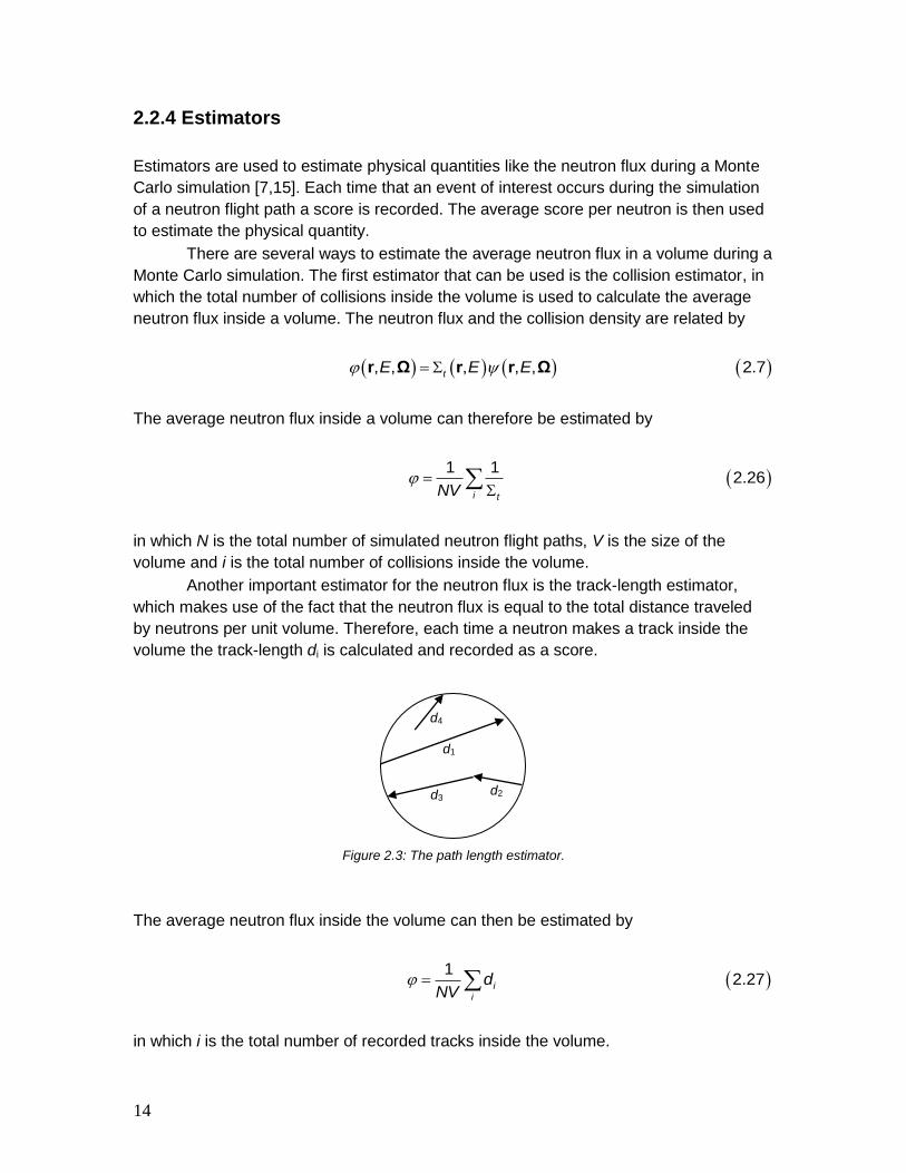
Another important estimator for the neutron flux is the track-length estimator,

which makes use of the fact that the neutron flux is equal to the total distance traveled

by neutrons per unit volume. Therefore, each time a neutron makes a track inside the

volume the track-length di is calculated and recorded as a score.

Figure 2.3: The path length estimator.

The average neutron flux inside the volume can then be estimated by

1

2.27i

i

dNV

in which i is the total number of recorded tracks inside the volume.

d1

d3 d2

d4

15

Reaction rates inside a volume can be estimated by using one of the neutron flux

estimators and multiplying the scores with the appropriate macroscopic cross-section.

For example the track-length estimator for the number of fission reactions is given by

1

2.28f f i

i

R dNV

in which Σf is the macroscopic fission cross-section and Rf is the reaction rate for fission.

Another important physical quantity is the multiplication factor keff which can be

estimated in several ways. First of all, it is possible to use the definition and calculate the

total number of neutrons in each successive generation.

number of neutrons in generation 1

2.1number of neutrons in generation

eff

ik

i

It is also possible to use one of the flux estimators by multiplying the scores with vΣf. The

collision estimator for keff is for example given by:

1

2.29 feff

i t

kN

in which ν is the average number of neutrons released during a fission reaction and i is

the total number of collisions inside the reactor.

2.2.5 Variance & variance reduction

During a Monte Carlo simulation the value of a physical quantity such as the neutron flux

is estimated by calculating the average total score per source neutron for the appropriate

estimator.

1

1 2.30

N

i

i

xN

Here N is the number of simulated neutrons and xi is the total score of the ith neutron.

Because the Monte Caro simulation is a stochastic process, there is always a

statistical error associated with the results [7,15]. A measure for the statistical error is the

variance σ2 which is a measure of how far the values of xi lie from the average value μ.

16

2

22 2

1 1 1

1 1 1 2.31

1 1

N N N

i i i

i i i

x x xN N N

The variance of the average value itself is given by

2

2 2 2

1 1

1 1 1 1 2.32

1

N N

i i

i i

x xN N N N

An important part of a Monte Carlo simulation is to reduce the variance in order

to improve the accuracy of the results of the Monte Carlo calculation. The easiest way to

do this is to increase the number of neutron simulations, but increasing the number of

neutron simulations also increases the computation time of the Monte Carlo simulation,

which is not always an option.

Another method to decrease the variance is to perform a non-analog Monte Carlo

simulation. During an analog Monte Carlo simulation all the neutron flight paths are

faithfully simulated, but in a non-analog Monte Carlo simulation we try to follow those

neutrons that have a large contribution to the physical quantities that need to be

estimated, for example by increasing the number of neutrons in regions of interest and

decreasing the number of neutrons in unimportant regions. To make sure that the

average score is the same as during an analog Monte Carlo simulation the scores are

modified. A statistical weight is assigned to each neutron and each score is weighted by

the statistical weight of the neutron.

One way to reduce the variance during a non-analog Monte Carlo simulation is to

alter the probability density functions to favor events of interest. This is called importance

sampling and every time an altered probability density functions is sampled the weight of

the neutron is adjusted.

Implicit capture is also a way to reduce the variance during a Monte Carlo

simulation. With implicit capture a neutron always survives a collision, but the weight of

the neutron is reduced with the probability that the neutron gets absorbed.

1 2.33anew

t

w w

Here w is the weight of the neutron before the collision and wnew is the weight of the

neutron after the collision. Implicit capture always decreases the variance per neutron

but it also increases the computation time of the Monte Carlo simulation.

Neutrons with a very low statistical weight contribute very little to the final results

of the Monte Carlo simulation. To prevent that these neutrons are continued to be

simulated, a game of Russian roulette can be played. When the weight w of a neutron

gets below a certain limit wRR then the game of Russian roulette is played in which the

probability Ps that the neutron survives is given by

17

2.34s

s

wP

w

If the neutron survives then it gets assigned a new survival weight ws, otherwise the

neutron is killed. Russian roulette always increases the variance but it does decrease the

computation time per neutron of the Monte Carlo simulation.

Another method to reduce the variance is called splitting. When the statistical

weight of a neutron exceeds a certain limit then the neutron is split into Ns identical

neutrons each with a weight of w/Ns. The new neutrons are then continued to be

followed and their scores are added up to that of the original neutron. Splitting always

decreases the variance but it does increase the computation time of the Monte Carlo

simulation.

The combination of Russian roulette and splitting is controlled by a weight

window which prevents that the weight of a neutron becomes too large or too small.

When the weight of a neutron is lower than a certain value than a game of Russian

roulette is played, and when the weight of the neutron is higher than a particular value

the neutron is split into several neutrons. The weight boundaries may be space and

energy depended and the importance can be used to generate the windows. This

method decreases the variance because of splitting but at the same time it also

decreases computation time of the Monte Carlo simulation because of Russian roulette.

2.3 The statistical geometry model

In order to be able to calculate the neutronics of a nuclear reactor with a Monte Carlo

code, it is necessary to know the exact geometry of the reactor. However, for a pebble

bed reactor the exact geometry is unknown because not only are the TRISO particles

randomly distributed inside the pebbles, but also are the pebbles themselves randomly

stacked inside the reactor.

The usual solution to this problem is to either model the core of the reactor as a

homogeneous mixture of the pebbles and the helium, or to first compute a randomly

stacked pebble bed. However, not all the effects of the pebble bed on the neutronics are

included when a homogenized core is used, and generating a large randomly stacked

pebble bed requires a considerable amount of computation time.

A way around these problems is to use a statistical geometry model in the Monte

Carlo code as described by Murata et al.[9,10]. During a Monte Carlo simulation the flight

path of a neutron in a pebble bed reactor consists of the neutron entering a pebble, the

transport of the neutron inside the pebble, the neutron exiting the pebble and the neutron

entering the next pebble. It is therefore not necessary to know the location of all the

pebbles in advance during the simulation of a neutron flight path, only the location of the

next pebble that a neutron is entering is necessary. This makes it possible during a

Monte Carlo simulation to arrange the pebbles one after another along a neutron flight

18

path using probability density functions to determine the location of the next pebble with

respect to the neutron flight path.

A statistical geometry model can also be used for the TRISO particles that are

randomly distributed throughout the fuel zone of each pebble. However, during this

research project the pebbles were modeled as spheres made of a homogeneous mixture

of the pebble material and TRISO particles and a statistical geometry model was only

used for the pebbles.

The simulation of a neutron flight path with a Monte Carlo code in which a

statistical geometry model is incorporated is as follows. Because the pebbles were

modeled as spheres made of a homogeneous mixture of the pebble material and TRISO

particles, inside each pebble the neutron flight path is simulated in the same way as

during a regular Monte Carlo simulation. However, things are different when a neutron

exits the pebble. In a regular Monte Carlo simulation the location of all the pebbles is

known, therefore, it is straightforward to calculate which pebble the neutron enters next,

and its flight path is continued in the new pebble. However, when a statistical geometry

model is used, first the distance that the neutron travels inside the void space is sampled

from a probability density function. This gives the location in the reactor where the

neutron enters the next pebble. Next, the incident angle of the neutron is sampled from a

second probability density function and is used to calculate the location of the next

pebble. The neutron flight path is then continued in the new pebble. In figure 2.4 a

schematic overview is given of the statistical geometry model.

There are still some questions left about using a statistical geometry model for

calculating the neutronics of a pebble bed reactor. Because probability density functions

are used to describe the streaming of the neutrons through the void space between the

pebbles some information about the pebble bed is lost, which could result in possible

errors in the calculations. Another issue is that the probability density function that is

used to calculate the distance that a neutron will travel in the void space depends on the

packing density of the pebble bed, which is not the same everywhere in the reactor

because of the influence the boundary of the reactor has on the pebble bed.

In this research project the accuracy of the statistical geometry model for the

analyses of a randomly stacked pebble bed reactor was examined, by comparing the

results from a Monte Carlo code in which a statistical geometry model is incorporated

with those of a regular Monte Carlo code. The influence of the absorption cross-section

and the packing density fluctuations near the boundary of the reactor as well as the

effect of using different probability density functions for two extra zones near the

boundary on the accuracy of the statistical geometry model was also investigated.

19

(a) Inside each pebble the neutron flight path is simulated in the normal way.

(b) When a neutron exits a pebble first the distance that the neutron travels in the void space is sampled.

(c) Then, the incident angle of the neutron is sampled.

(d) Finally, the neutron flight path is continued inside the new pebble.

Figure 2.4: A schematic representation of the statistical geometry model.

α

20

21

Chapter 3

The Monte Carlo codes

During this research project, two basic Monte Carlo neutron transport codes were written

in order to examine the accuracy of the statistical geometry model for the analyses of a

randomly stacked pebble bed reactor. Both Monte Carlo codes use only one energy

group and the only neutron interactions that are considered are isotropic scattering,

capture and fission. The first Monte Carlo code that was written is called MC-Fixed and

uses a pre-generated pebble bed for its calculations. This code is used to calculate the

probability density functions for the statistical geometry model, and is also used as a

benchmark for the second code that was written. This code is called MC-SGM and uses

a statistical geometry model for its calculations.

3.1 The Monte Carlo code MC-Fixed

3.1.1 General overview of the Monte Carlo code

This program starts with generating the pebble locations of the pebble bed. For a regular

pebble bed stacking (e.g. simple cubic, hexagonal close-packed), the coordinates of the

pebbles are generated by the program itself. For a randomly stacked pebble bed, the

pebble bed stacking is generated by another program written by G. J. Auwerda which

uses the expanding system method [11].

All the Monte Carlo calculations were performed for an infinite cylinder, so for the

calculations only a section of the generated pebble bed between zmin and zmax is used,

and reflecting boundary conditions are imposed on the top and bottom surface of the

used pebble bed section, see figure 3.1. The pebbles were modeled as spheres with a

radius of 3 cm and made of a homogeneous mixture of the pebble material and TRISO

particles. No reflector was included in the model and a vacuum boundary condition was

imposed at the side wall of the reactor.

22

Figure 3.1: A side view (left) and above view (right) of the used pebble bed section.

After the pebble bed is generated, the Monte Carlo simulation is started. The

criticality of the reactor is calculated by simulating successive fission cycles. For the first

cycle, the starting location of the neutrons is sampled from a uniform distribution. The

flight path of each neutron is then simulated in the normal way. When during the

simulation a fission reaction occurs, the location where the fission neutrons are born is

stored. These are then used as starting locations for the next cycle. For every cycle the

value of keff is calculated using a collision estimator. When after a number of cycles the

value of keff stabilizes, the fission source has converged, and the average value of keff of

all subsequent cycles is used to estimate the criticality of the reactor. After the fission

source has converged the radial flux profile is also measured during all subsequent

cycles. For this purpose the volume of the reactor is divided up in a large number of

cylindrical shells and the average neutron flux inside each volume is calculated with a

track-length estimator.

3.1.2 The simulation of a neutron flight path

The first step into simulating the flight path of each neutron is to sample a starting

location and direction for the neutron. For the first cycle the starting location of each

neutron is determined by randomly sampling a pebble from the pebble bed, and then

randomly sampling a point inside that pebble. For the other cycles the starting location of

each neutron is the location where a fission neutron was born in the previous cycle. After

the starting location of a neutron has been determined the direction of the neutron is

sampled using an isotropic distribution.

zmax

zmin

23

zmax

dpeb

dwall

dTB

zmin

After the starting location and direction of a neutron have been sampled the flight

path of the neutron is simulated. First the distance that the neutron will travel before

undergoing an interaction is sampled. It is then checked whether the neutron can travel

such a distance without exiting either the pebble or the pebble bed section. This is done

by calculating the distance to the surface of the pebble, and the distances to the plane

through either zmin or zmax, depending on the direction of the neutron, and the boundary

of the reactor, and comparing these with the sampled distance to the next interaction.

Figure 3.2: The three distances that are calculated by MC-Fixed.

If the distance to the surface of the pebble, dpeb, is the shortest one, the neutron

exits the pebble and the code calculates if the neutron enters another pebble or leaks

out of the reactor. If the neutron enters another pebble, its flight path is continued in the

new pebble. During the active cycles the distance that the neutron travels in the void

space between the pebbles is calculated and stored. These values are later used to

calculate the probability density function for the statistical geometry model. If the neutron

does not enter another pebble, it leaks out of the reactor and the simulation of its flight

path is stopped.

If the distance to the side wall of the reactor, dwall, is the shortest one, the neutron

leaks out of the reactor before exiting the pebble, and its flight path is stopped. This can

only happen with geometries where partial pebbles at the boundary of the reactor are

allowed.

If the distance to the horizontal plane at either the top or bottom surface of the

pebble bed section, dTB, is the shortest one then the neutron is reflected at the surface

and its flight path is continued.

If the sampled distance to the next interaction, dint, is the shortest one, the

neutron is moved to the location of its next collision, and the type of interaction is

sampled. If the interaction is a scattering event, the new direction of the neutron is

24

sampled and the neutron is continued to be followed. If, however, the neutron gets

captured during the event, the simulation of the neutron flight path is stopped. If the

interaction was a fission event, the number of neutrons that are released during the

fission reaction is sampled and their location is stored. Figure 3.3 gives a schematic

overview of the simulation of a neutron flight path in MC-Fixed.

Figure 3.3: Schematic overview of the simulation of a neutron flight path in MC-Fixed.

No

Yes

No

Yes No

Yes

Sample a location

Sample the direction

Sample the interaction

Sample/calculate distances

Scatter event? Fission event? Sample number of neutrons

and store their location

Dm = dint?

Yes

Dm = minimum(dint, dpeb, dTB, dwall)

Dm = dTB?

Move the neutron to

the next location

Capture event

No

Dm = dpeb?

No

Yes

Reflect the neutron at the

surface

No

Move the neutron to the

next pebble

Stop neutron flight path

The neutron leaks out

of the system

Enters another

pebble?

Calculate if the neutron

enters a new pebble

Yes

25

3.1.3 Validation of MC-Fixed

In order to check the accuracy of MC-Fixed a benchmark calculation was performed.

The criticality of three randomly stacked pebble bed reactors was calculated with both

MC-Fixed and the Monte Carlo code KENO [16]. The calculations with KENO were

performed by G. J. Auwerda and the cross-sections that were used for the calculations

are given here below in table 3.1.

Table 3.1: The parameters of the system.

Σt 0.381109 cm-1

Σa 0.00316019 cm-1

Σf 0.00198721 cm-1

ν 2.43722

Before the criticality calculations were performed, it was first tested if the fission

source converges during a calculation with MC-Fixed. This was done by performing a

criticality calculation with MC-Fixed and determining whether the value of keff stabilizes

after a number of cycles. In figure 3.4 both the value of keff of each cycle as well as the

average value of keff up to that cycle are plotted for a criticality calculation of a randomly

stacked pebble bed reactor with a radius of 90 cm.

Figure 3.4: keff as a function of the cycle for a criticality calculation with MC-Fixed.

Figure 3.4 shows that during the criticality calculation with MC-Fixed the fission source

quickly converges and that the value of keff remains stable during all subsequent cycles.

26

The results of the criticality calculations of the three randomly stacked pebble bed

reactors are given here below in table 3.2.

Table 3.2: The results of the validation of MC-Fixed.

Radius of the reactor

KENO MC-Fixed Relative Error

15 cm 0.10250 ± 0.00012 0.10253 ± 0.00010 0.029% 50 cm 0.58476 ± 0.00027 0.58467 ± 0.00043 -0.015% 90 cm 0.99070 ± 0.00038 0.99127 ± 0.00085 0.057%

As can be seen in table 3.1 the values for keff are in excellent agreement with each other,

which gives us the confidence that the Monte Carlo code MC-Fixed works correctly.

3.2 The Monte Carlo code MC-SGM

After the Monte Carlo code MC-Fixed was written, a copy of the code was modified to

use a statistical geometry model for its calculations. For the initial cycle the starting

location of each neutron is now determined by first randomly sampling a location for the

pebble, and then randomly sampling a point inside that pebble. For all the subsequent

cycles the starting location of each neutron is again a location where a fission neutron

was born in the previous cycle.

After the starting location and direction of a neutron have been sampled, the flight

path of the neutron is simulated. Inside each pebble the neutron flight path is simulated

in the same way as in MC-Fixed. However, things are different when a neutron exits the

pebble. First, the distance that the neutron travels in the void space between the pebbles

is sampled from a probability density function. This gives the location where the neutron

enters the next pebble. It is then checked whether this location is inside the reactor. If so,

then the incident angle of the neutron is sampled from a cosine distribution, and the

location of the next pebble is calculated. If not then the neutron leaks out of the reactor

and the neutron flight path is stopped. If a pebble was generated it is checked by the

code whether the pebble is inside the reactor. If so, then the neutron is moved to the

new location and the neutron flight path is continued in the new pebble. If not then the

neutron leaks out of the reactor and the neutron flight path is stopped. On the next page

a schematic overview of the simulation of a neutron flight path in the MC-SGM code is

given in figure 3.5.

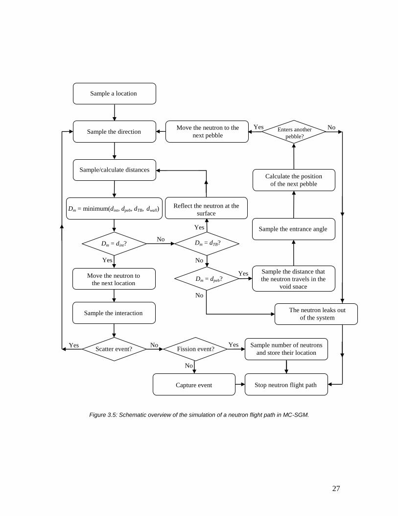
27

Figure 3.5: Schematic overview of the simulation of a neutron flight path in MC-SGM.

No

Yes

No

Yes No

Yes

Sample a location

Sample the direction

Sample the interaction

Sample/calculate distances

Scatter event? Fission event? Sample number of neutrons

and store their location

Dm = dint?

Yes

Dm = minimum(dint, dpeb, dTB, dwall)

Dm = dTB?

Move the neutron to

the next location

Capture event

No

Dm = dpeb?

No

Yes

Reflect the neutron at the

surface

No Move the neutron to the

next pebble

Stop neutron flight path

The neutron leaks out

of the system

Enters another

pebble?

Calculate the position

of the next pebble

Sample the entrance angle

Sample the distance that

the neutron travels in the

void space

Yes

28

29

Chapter 4

Results

In this chapter the results are presented of this research project. Section 4.1 is used to

present the probability density functions for the distance that a neutron travels in the void

space between the pebbles, and for the incident angle distribution of the neutrons. Both

are necessary for the statistical geometry model that is used in MC-SGM. As a first test

for the statistical geometry model and MC-SGM, the criticality (keff) of several pebble bed

reactors with an ordered pebble bed stacking is calculated in section 4.2. To investigate

the accuracy of the statistical geometry for the analyses of a randomly stacked pebble

bed reactor, the criticality of several randomly stacked pebble bed reactors is calculated

in section 4.3. Then, in section 4.4 the influence of the absorption cross-section on the

accuracy of the statistical geometry model is investigated by calculating the criticality of a

pebble bed reactor with a HCP pebble bed stacking using several different values for the

absorption cross-section. Finally, the influence of the packing fraction fluctuations in a

randomly stacked pebble bed reactor on the accuracy of the results is investigated in

section 4.5, as well as the possibility to use different probability density functions for

different zones in the pebble bed to improve the accuracy of the statistical geometry

model.

4.1 The probability density functions

In the statistical geometry model probability density functions are used to calculate the

distance that a neutron travels in the void space between the pebbles when it exits a

pebble, and what the orientation of the next pebble is with respect to the neutrons flight

path. Both probability density functions were calculated during the criticality calculations

with the Monte Carlo code MC-Fixed. The results of the calculations are presented in

this section.

30

4.1.1 The entrance angle distribution

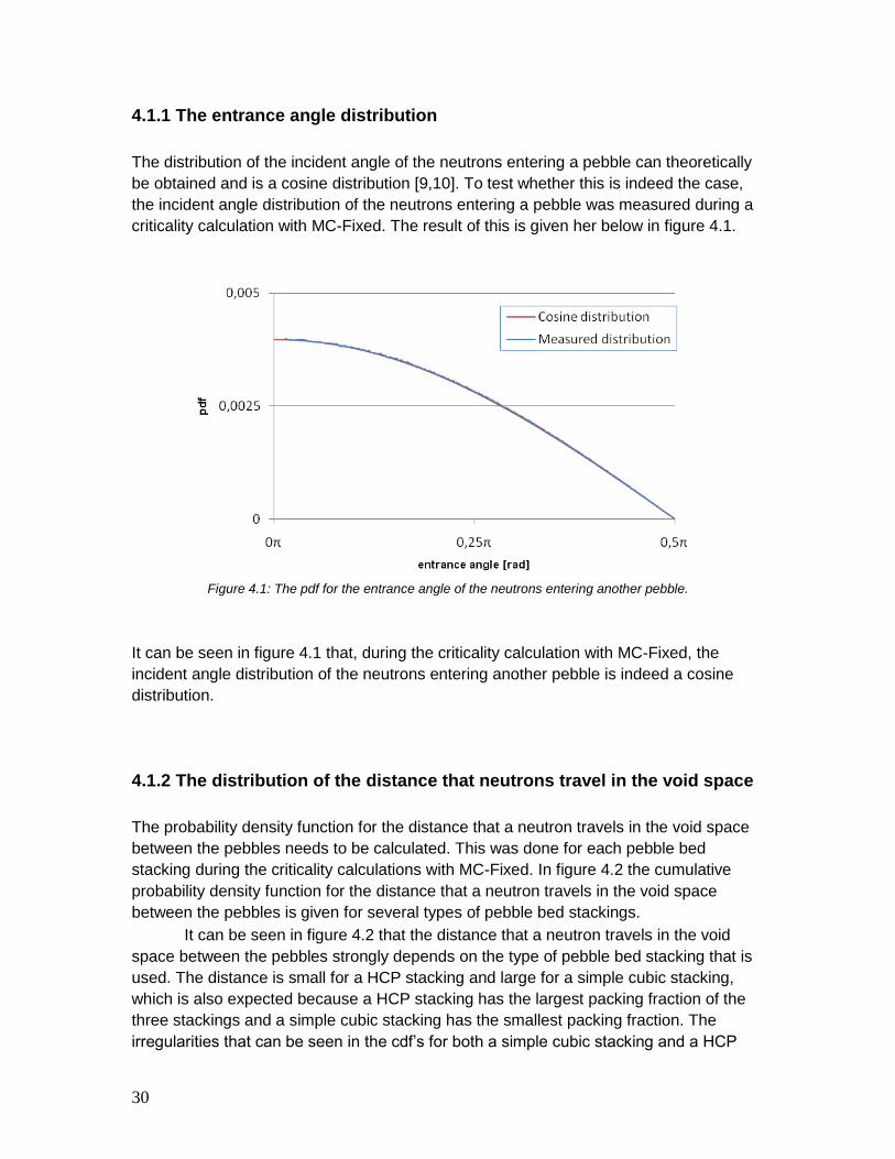
The distribution of the incident angle of the neutrons entering a pebble can theoretically

be obtained and is a cosine distribution [9,10]. To test whether this is indeed the case,

the incident angle distribution of the neutrons entering a pebble was measured during a

criticality calculation with MC-Fixed. The result of this is given her below in figure 4.1.

Figure 4.1: The pdf for the entrance angle of the neutrons entering another pebble.

It can be seen in figure 4.1 that, during the criticality calculation with MC-Fixed, the

incident angle distribution of the neutrons entering another pebble is indeed a cosine

distribution.

4.1.2 The distribution of the distance that neutrons travel in the void space

The probability density function for the distance that a neutron travels in the void space

between the pebbles needs to be calculated. This was done for each pebble bed

stacking during the criticality calculations with MC-Fixed. In figure 4.2 the cumulative

probability density function for the distance that a neutron travels in the void space

between the pebbles is given for several types of pebble bed stackings.

It can be seen in figure 4.2 that the distance that a neutron travels in the void

space between the pebbles strongly depends on the type of pebble bed stacking that is

used. The distance is small for a HCP stacking and large for a simple cubic stacking,

which is also expected because a HCP stacking has the largest packing fraction of the

three stackings and a simple cubic stacking has the smallest packing fraction. The

irregularities that can be seen in the cdf’s for both a simple cubic stacking and a HCP

31

stacking are the result of the regular structure of both pebble bed stackings, and are

therefore not present in the cdf for a randomly stacked pebble bed.

Figure 4.2: The cdf for the distance that a neutron travels in the void space between the pebbles for a simple

cubic stacking, a hexagonal close-packed stacking and a random stacking.

4.2 Ordered pebble bed stackings

As a first test for both the statistical geometry model and the Monte Carlo code MC-SGM,

the criticality of several pebble bed reactors with an ordered pebble bed stacking was

calculated with MC-Fixed and MC-SGM. However, first it is tested in section 4.2.1 if the

fission source converges during a criticality calculation with MC-SGM. The results of the

criticality calculations are then presented in section 4.2.2. To investigate the problem that

occurs for a reactor with a simple cubic stacking, the boundary condition for MC-SGM is

changed, and the criticality of the reactors is recalculated with MC-SGM in section 4.2.3.

Finally, in section 4.2.4 the conclusions for this subchapter are presented.

4.2.1 Testing for convergence of the fission source in MC-SGM

Before the criticality calculations were performed with MC-SGM, it was first tested if the

fission source converges during a criticality calculation with MC-SGM. This was done by

performing a criticality calculation with MC-SGM and determining whether the value of

keff stabilizes after a number of cycles. During the calculation the fission source density

for each cycle was measured and the cross-sections that were used for the calculation

32

are given in table 4.1. In figure 4.3 both the keff of each cycle and the average value of

keff up to that cycle are plotted as a function of the fission cycle for a criticality calculation

of a reactor with a HCP stacking and a radius of 70 cm. In figure 4.4 the fission source

density is plotted for three different fission cycles.

Table 4.1: The cross-sections.

Σt 0.381109 cm-1

Σa 0.00316019 cm-1

Σf 0.00198721 cm-1

ν 2.43722

Figure 4.3: keff and the average value of keff as a function of the fission cycle.

Figure 4.4: The fission source for three different cycles.

33

In can be seen in figure 4.3 that during the criticality calculation with MC-SGM the fission

source quickly converges and that the value of keff remains stable during all subsequent

cycles. Figure 4.4 shows that the fission source remains stable during the active cycles.

4.2.2 The criticality calculations

4.2.2.1 A simple cubic pebble bed stacking

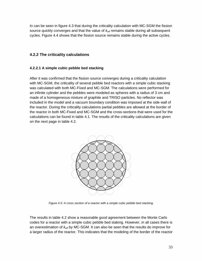
After it was confirmed that the fission source converges during a criticality calculation

with MC-SGM, the criticality of several pebble bed reactors with a simple cubic stacking

was calculated with both MC-Fixed and MC-SGM. The calculations were performed for

an infinite cylinder and the pebbles were modeled as spheres with a radius of 3 cm and

made of a homogeneous mixture of graphite and TRISO particles. No reflector was

included in the model and a vacuum boundary condition was imposed at the side wall of

the reactor. During the criticality calculations partial pebbles are allowed at the border of

the reactor in both MC-Fixed and MC-SGM and the cross-sections that were used for the

calculations can be found in table 4.1. The results of the criticality calculations are given

on the next page in table 4.2.

Figure 4.5: A cross section of a reactor with a simple cubic pebble bed stacking.

The results in table 4.2 show a reasonable good agreement between the Monte Carlo

codes for a reactor with a simple cubic pebble bed staking. However, in all cases there is

an overestimation of keff by MC-SGM. It can also be seen that the results do improve for

a larger radius of the reactor. This indicates that the modeling of the border of the reactor

34

in MC-SGM is not entirely correct. In order to confirm this, the two radial flux profiles that

were calculated for a reactor with a radius of 70 cm are plotted in figure 4.6.

Table 4.2: The calculated values for keff for several reactors with a simple cubic stacking.

Radius of the reactor

MC-Fixed MC-SGM Relative Error

30 cm 0.22930 ± 0.00054 0.23979 ± 0.00041 4.574% 50 cm 0.46041 ± 0.00047 0.46878 ± 0.00049 1.817% 70 cm 0.67396 ± 0.00061 0.68496 ± 0.00069 1.632% 90 cm 0.85176 ± 0.00080 0.86075 ± 0.00100 1.055% 120 cm 1.04700 ± 0.00104 1.05707 ± 0.00119 0.961%

Figure 4.6: The radial flux profiles for a reactor with a simple cubic stacking and a radius of 70 cm.

It can be seen in figure 4.6 that for most of the core volume the two radial flux profiles

are in reasonably good agreement with each other. The only exception is close to the

boundary of the core where the radial flux profile that was calculated with MC-SGM is

considerably higher than the radial flux profile that was calculated with MC-Fixed. This

shows that the neutron leakage was underestimated by MC-SGM which resulted in an

overestimation of keff. This confirms that the modeling of the boundary of the reactor in

MC-SGM is indeed not entirely correct, and also indicates that there is an overestimation

of the pebble density near the boundary of the reactor by MC-SGM. It can therefore be

concluded that the boundary condition that was used during the criticality calculations

with MC-SGM is not correct for a reactor with a simple cubic pebble bed stacking.

35

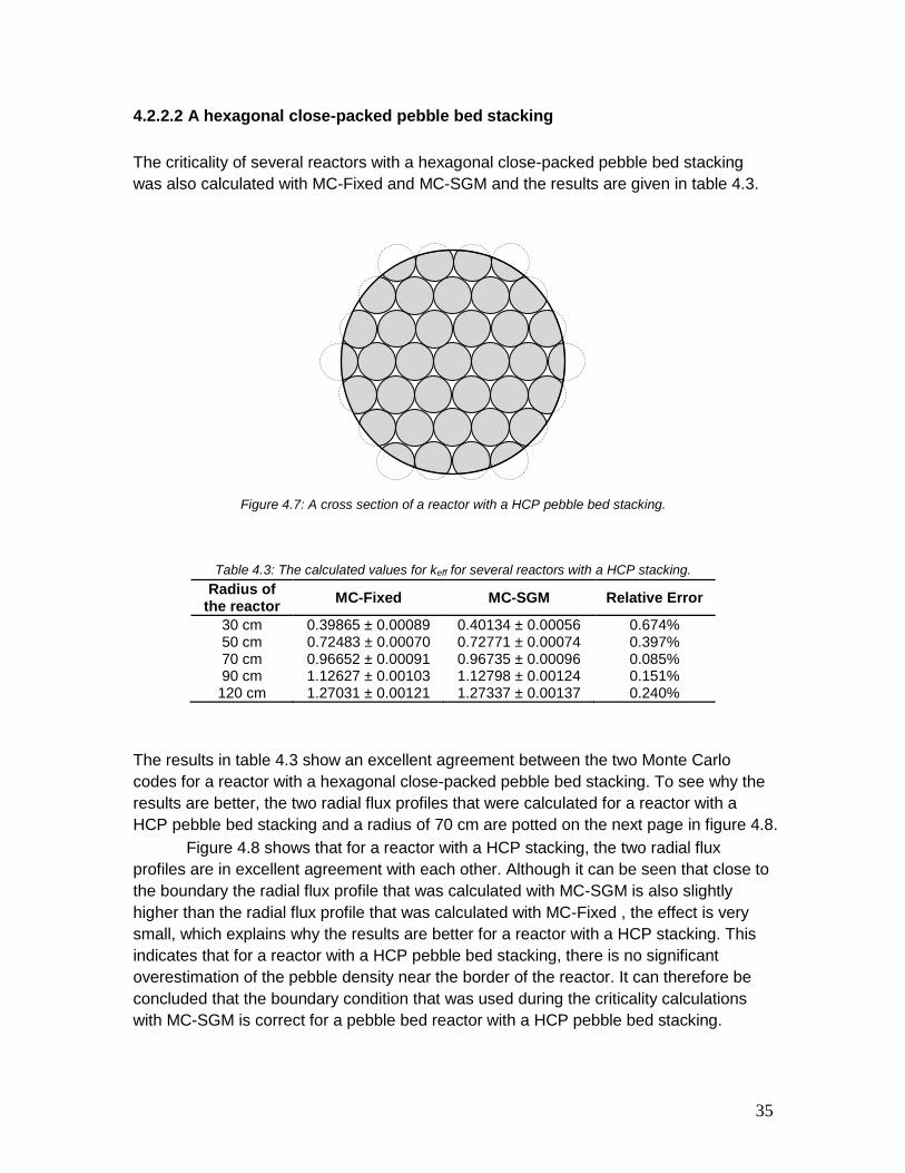
4.2.2.2 A hexagonal close-packed pebble bed stacking

The criticality of several reactors with a hexagonal close-packed pebble bed stacking

was also calculated with MC-Fixed and MC-SGM and the results are given in table 4.3.

Figure 4.7: A cross section of a reactor with a HCP pebble bed stacking.

Table 4.3: The calculated values for keff for several reactors with a HCP stacking.

Radius of the reactor

MC-Fixed MC-SGM Relative Error

30 cm 0.39865 ± 0.00089 0.40134 ± 0.00056 0.674% 50 cm 0.72483 ± 0.00070 0.72771 ± 0.00074 0.397% 70 cm 0.96652 ± 0.00091 0.96735 ± 0.00096 0.085% 90 cm 1.12627 ± 0.00103 1.12798 ± 0.00124 0.151% 120 cm 1.27031 ± 0.00121 1.27337 ± 0.00137 0.240%

The results in table 4.3 show an excellent agreement between the two Monte Carlo

codes for a reactor with a hexagonal close-packed pebble bed stacking. To see why the

results are better, the two radial flux profiles that were calculated for a reactor with a

HCP pebble bed stacking and a radius of 70 cm are potted on the next page in figure 4.8.

Figure 4.8 shows that for a reactor with a HCP stacking, the two radial flux

profiles are in excellent agreement with each other. Although it can be seen that close to

the boundary the radial flux profile that was calculated with MC-SGM is also slightly

higher than the radial flux profile that was calculated with MC-Fixed , the effect is very

small, which explains why the results are better for a reactor with a HCP stacking. This

indicates that for a reactor with a HCP pebble bed stacking, there is no significant

overestimation of the pebble density near the border of the reactor. It can therefore be

concluded that the boundary condition that was used during the criticality calculations

with MC-SGM is correct for a pebble bed reactor with a HCP pebble bed stacking.

36

Figure 4.8: The radial flux profiles for a reactor with a HCP pebble bed stacking and a radius of 70 cm.

4.2.3 Recalculation of the criticality with MC-SGM

4.2.3.1 A simple cubic pebble bed stacking

To confirm that the problem for a reactor with a simple cubic pebble bed stacking is an

overestimation of the pebble density near the boundary of the reactor by MC-SGM, the

boundary condition for MC-SGM was changed in order to reduce the pebble density

near the boundary of the reactor, and the criticality of the reactors was recalculated with

MC-SGM. During the calculations with MC-SGM, the pebbles are still allowed to be

partially outside the reactor, but the center of each pebble now has to be inside the

reactor. If a pebble is generated with its centre outside the reactor, it is discarded and

the neutron leaks out of the reactor. The results of the new criticality calculations with

MC-SGM are given in table 4.4.

Table 4.4: The recalculated values for keff for several reactors with a simple cubic stacking.

Radius of the reactor

MC-Fixed MC-SGM Relative Error

30 cm 0.22930 ± 0.00054 0.23043 ± 0.00027 0.492% 50 cm 0.46041 ± 0.00047 0.45917 ± 0.00048 -0.269% 70 cm 0.67396 ± 0.00061 0.67458 ± 0.00068 0.091% 90 cm 0.85176 ± 0.00080 0.85418 ± 0.00084 0.284% 120 cm 1.04700 ± 0.00104 1.05048 ± 0.00095 0.332%

37

Table 4.4 shows that with the new boundary condition for MC-SGM, the results for a

reactor with a simple cubic pebble bed stacking have significantly improved. In order to

confirm this, the radial flux profiles that were calculated for a reactor with a simple cubic

pebble bed stacking and a radius of 70 cm are plotted in figure 4.9.

Figure 4.9: The radial flux profiles for a reactor with a simple cubic stacking and a radius of 70 cm.

Figure 4.9 shows that with the new boundary condition for MC-SGM, the two radial flux

profiles are now in better agreement with each other. Although it can be seen that at the

boundary of the reactor the radial flux profile that was calculated with MC-SGM is still

slightly higher than the radial flux profile that was calculated with MC-Fixed, the effect is

smaller which explains why the results are now better. It can therefore be concluded that

the problem for a reactor with a simple cubic stacking is indeed an overestimation of the

pebble density near the boundary of the reactor by MC-SGM, and also that the new

boundary condition for MC-SGM largely solves this problem.

4.2.3.2 A HCP pebble bed stacking

To test whether the new boundary condition for MC-SGM also gives a good result for a

reactor with a HCP pebble bed stacking, the criticality of the reactors with a HCP pebble

bed stacking was recalculated with MC-SGM and the new boundary condition. The

results are given on the next page in table 4.5.

Table 4.5 shows that with the new boundary condition for MC-SGM, the accuracy

of the results for a reactor with a HCP pebble bed stacking has decreased, and in all

cases there now is an underestimation of keff by MC-SGM. This indicates that with the

38

new boundary condition for MC-SGM, there is now an underestimation of the pebble

density near the boundary of the reactor by MC-SGM. To confirm this, the radial flux

profiles that were calculated for a reactor with a radius of 70 cm are plotted in figure 4.10.

Table 4.5: The recalculated values for keff for several reactors with a HCP pebble bed stacking.

Radius of the reactor

MC-Fixed MC-SGM Relative Error

30 cm 0.39865 ± 0.00089 0.38561 ± 0.00042 -3.271% 50 cm 0.72483 ± 0.00070 0.71556 ± 0.00071 -1.278% 70 cm 0.96652 ± 0.00091 0.95919 ± 0.00090 -0.758% 90 cm 1.12627 ± 0.00103 1.12269 ± 0.00124 -0.317% 120 cm 1.27031 ± 0.00121 1.26831 ± 0.00113 -0.157%

Figure 4.10: The radial flux profiles for a reactor with a HCP stacking and a radius of 70 cm.

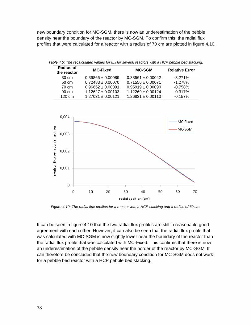
It can be seen in figure 4.10 that the two radial flux profiles are still in reasonable good

agreement with each other. However, it can also be seen that the radial flux profile that

was calculated with MC-SGM is now slightly lower near the boundary of the reactor than

the radial flux profile that was calculated with MC-Fixed. This confirms that there is now

an underestimation of the pebble density near the border of the reactor by MC-SGM. It

can therefore be concluded that the new boundary condition for MC-SGM does not work

for a pebble bed reactor with a HCP pebble bed stacking.

39

4.2.4 Conclusions

Based on the results in this paragraph, it can be concluded that both the statistical

geometry model and the Monte Carlo code MC-SGM work correctly for a pebble bed

reactor with an ordered pebble bed stacking, and give accurate results for both the

criticality of the reactor and the radial flux profile. However, the results also show that the

boundary condition that needs to be imposed for a criticality calculation with MC-SGM

depends on the type of pebble bed stacking that is used. Further research to find the

optimum boundary condition for both ordered pebble bed stackings could be useful.

4.3 Randomly stacked pebble beds

The main goal of this research project is to examine the accuracy of the statistical

geometry model for the analyses of a randomly stacked pebble bed reactor. This was

done by calculating the criticality of several randomly stacked pebble bed reactors with

MC-Fixed and MC-SGM, and comparing the results from both codes. The results of the

criticality calculations are given in section 4.3.1. To investigate if the accuracy of the

results can be improved by allowing partial pebbles to be generated at the boundary of

the reactor during the calculations with MC-SGM, the boundary condition for MC-SGM is

changed, and the criticality of the reactors is recalculated with MC-SGM in section 4.3.2.

Then, in section 4.3.3 it is investigated if the accuracy of the statistical geometry model

can be further improved by using another boundary condition for MC-SGM. Finally, in

section 4.3.4 the conclusions of this subchapter are presented.

4.3.1 The criticality calculations

To investigate the accuracy of the statistical geometry model for the analyses of a

randomly stacked pebble bed reactor, the criticality of several randomly stacked pebble

bed reactors was calculated with both MC-Fixed and MC-SGM. The calculations were

performed for an infinite cylinder and the pebbles were modeled as spheres made of a

homogeneous mixture of graphite and TRISO particles. No reflector was included in the

model and a vacuum boundary condition was imposed at the side wall of the reactor.

Because partial pebbles are not allowed in the random pebble bed stackings that were

generated for MC-Fixed, there are no partial pebbles allowed at the border of the reactor

during the calculations with MC-SGM. The cross-sections that were used for the

calculations can be found in table 4.1. The results of the criticality calculations are given

in table 4.6 on the next page.

40

Table 4.6: The results of the criticality calculations for a randomly stacked pebble bed.

Radius of the reactor

MC-Fixed MC-SGM Relative Error

15 cm 0.10349 ± 0.00012 0.07908 ± 0.00015 -23.58% 27 cm 0.24984 ± 0.00030 0.21796 ± 0.00033 -12.76% 50 cm 0.58786 ± 0.00058 0.55404 ± 0.00070 -5.753% 90 cm 1.00991 ± 0.00061 0.98922 ± 0.00097 -2.048% 120 cm 1.18289 ± 0.00115 1.16982 ± 0.00148 -1.104%

The results in table 4.6 show that, especially for a small reactor, there is a significant

underestimation of keff by MC-SGM. It can also be seen that the results do improve for a

larger radius of the reactor. This indicates that the problem lies with the modeling of the

boundary of the reactor in MC-SGM. In order to confirm this, the two radial flux profiles

that were calculated for a reactor with a radius of 50 cm are plotted in figure 4.11.

Figure 4.11: The radial flux profiles for a randomly stacked pebble bed reactor with a radius of 50 cm.

As can be seen in figure 4.11, the two radial flux profiles do not correspond well with

each other. The radial flux profile that was calculated with MC-SGM is, especially near

the boundary of the reactor, considerably lower than the radial flux profile that was

calculated with MC-Fixed. This shows that the neutron leakage was overestimated by

MC-SGM which resulted in an underestimation of keff. This confirms that the problem lies

with the modeling of the boundary of the reactor in MC-SGM, and also shows that there

is a considerable underestimation of the pebble density near the boundary of the reactor

by MC-SGM. It can therefore be concluded that this boundary condition for MC-SGM is

not correct for a randomly stacked pebble bed reactor, and results in a considerable

underestimation of keff by MC-SGM.

41

4.3.2 Recalculation of keff with a different boundary condition for MC-SGM

The boundary condition that was used in the previous section resulted in a considerable

underestimation of keff by MC-SGM. The solution to this problem that was found by

Murata et al.[9,10] is to allow partial pebbles to be generated near the boundary of the

reactor during the calculations with MC-SGM. This way, the pebble density near the

boundary of the reactor is increased during the calculations with MC-SGM. In order to

investigate if this new boundary condition indeed improves the results, the boundary

condition for MC-SGM is changed, and the criticality of the reactors is recalculated with

MC-SGM. The results are given in table 4.7.

Table 4.7: The results of the criticality calculations with a different boundary condition for MC-SGM.

Radius of the reactor

MC-Fixed MC-SGM Relative Error

15 cm 0.10349 ± 0.00012 0.11604 ± 0.00019 12.12% 27 cm 0.24984 ± 0.00030 0.26806 ± 0.00044 7.292% 50 cm 0.58786 ± 0.00058 0.60260 ± 0.00080 2.507% 90 cm 1.00991 ± 0.00061 1.01609 ± 0.00086 0.611% 120 cm 1.18289 ± 0.00115 1.18501 ± 0.00150 0.179%

Table 4.7 shows that the results have indeed improved, and for the two largest reactors

the results are now in good agreement with each other. However, it can also be seen

that for a small reactor there now is a significant overestimation of keff by MC-SGM. This

indicates that, especially for a small pebble bed reactor, there now is an overestimation

of the pebble density near the boundary of the reactor by MC-SGM. In order to confirm

this, the two radial flux profiles that were calculated for a reactor with a radius of 50 cm

are plotted in figure 4.12 on the next page.

Figure 4.12 shows that with the new boundary condition for MC-SGM the two

radial flux profiles are now in reasonably good agreement which each other. However, it

can also be seen that, especially near the boundary of the reactor, the radial flux profile

that was calculated with MC-SGM is now higher than the radial flux profile that was

calculated with MC-Fixed. This confirms that there now is an overestimation of the

pebble density at the boundary of the reactor by MC-SGM which results in an under-

estimation of the neutron leakage and an overestimation of kef. It can therefore be

concluded that by allowing partial pebbles to be generated at the boundary of the reactor

during the calculations with MC-SGM the accuracy of the results indeed improves, and

gives good results for a large randomly stacked pebble bed reactor. However, for a small

pebble bed reactor this boundary condition results in a considerable overestimation of

keff by MC-SGM.

42

Figure 4.12: The radial flux profiles for a randomly stacked pebble bed reactor with a radius of 50 cm.

4.3.3 Testing a third boundary condition for MC-SGM

Next, it is investigated whether the results can be further improved by using a different

boundary condition for MC-SGM. If no partial pebbles are allowed to be generated at the

border of the reactor in MC-SGM, the pebble density near the border of the reactor is

underestimated. If, however, partial pebbles are allowed at the border of the reactor, the

pebble density near the border of the reactor is overestimated by MC-SGM. Therefore,

the boundary condition of section 4.2.3 that gave good results for a pebble bed reactor

with a simple cubic stacking is tried. During the calculations with MC-SGM, the pebbles

are allowed to be partially outside the reactor, but the center of each pebble still has to

be inside the reactor. If a pebble is generated with its centre outside the reactor, it is

discarded and the neutron leaks out of the reactor. The criticality of the randomly

stacked pebble bed reactors was recalculated, and the results are given in table 4.8

Table 4.8: The results of the criticality calculations with a third boundary condition for MC-SGM.

Radius of the reactor

MC-Fixed MC-SGM Relative Error

15 cm 0.10349 ± 0.00012 0.10680 ± 0.00019 3.198% 27 cm 0.24984 ± 0.00030 0.25558 ± 0.00040 2.297% 50 cm 0.58786 ± 0.00058 0.59033 ± 0.00081 0.420% 90 cm 1.00991 ± 0.00061 1.01089 ± 0.00097 0.097% 120 cm 1.18289 ± 0.00115 1.18419 ± 0.00150 0.109%

43

Table 4.8 shows that the results are now in reasonably good agreement with each other

for a small reactor, while for a large reactor the results have also slightly improved and

are in excellent agreement with each other. However, it can also be seen that for a small

reactor there is still a small overestimation of keff by MC-SGM. This indicates that there is

still a slight overestimation of the pebble density near the border by MC-SGM. In order to

confirm this, in figure 4.13 the two radial flux profiles are plotted that were calculated for

a pebble bed reactor with a radius of 50 cm.

Figure 4.13: The radial flux profiles for a random pebble bed reactor with a radius of 50 cm.

Figure 4.13 shows that for most of the reactor the radial flux profiles are now in excellent

agreement with each other. However, it can also be seen that the radial flux profile that

was calculated with MC-SGM is still slightly higher near the border of the reactor than

the radial flux profile that was calculated with MC-Fixed. This confirms that there is still a

slight overestimation of the pebble density near the border of the reactor. It can therefore

be concluded that this boundary condition for MC-SGM gives more accurate results than

the two previous boundary conditions. However, for a small reactor there is still a slight

overestimation of keff by MC-SGM so this boundary condition is also not entirely correct.

4.3.4 Conclusions

Based on the results in this paragraph, it can be concluded that the statistical geometry

model works for a randomly stacked pebble bed reactor, and gives reasonably good

results for a small reactor and excellent results for a large reactor. Allowing partial

pebbles to be generated at the border of the reactor during the criticality calculations

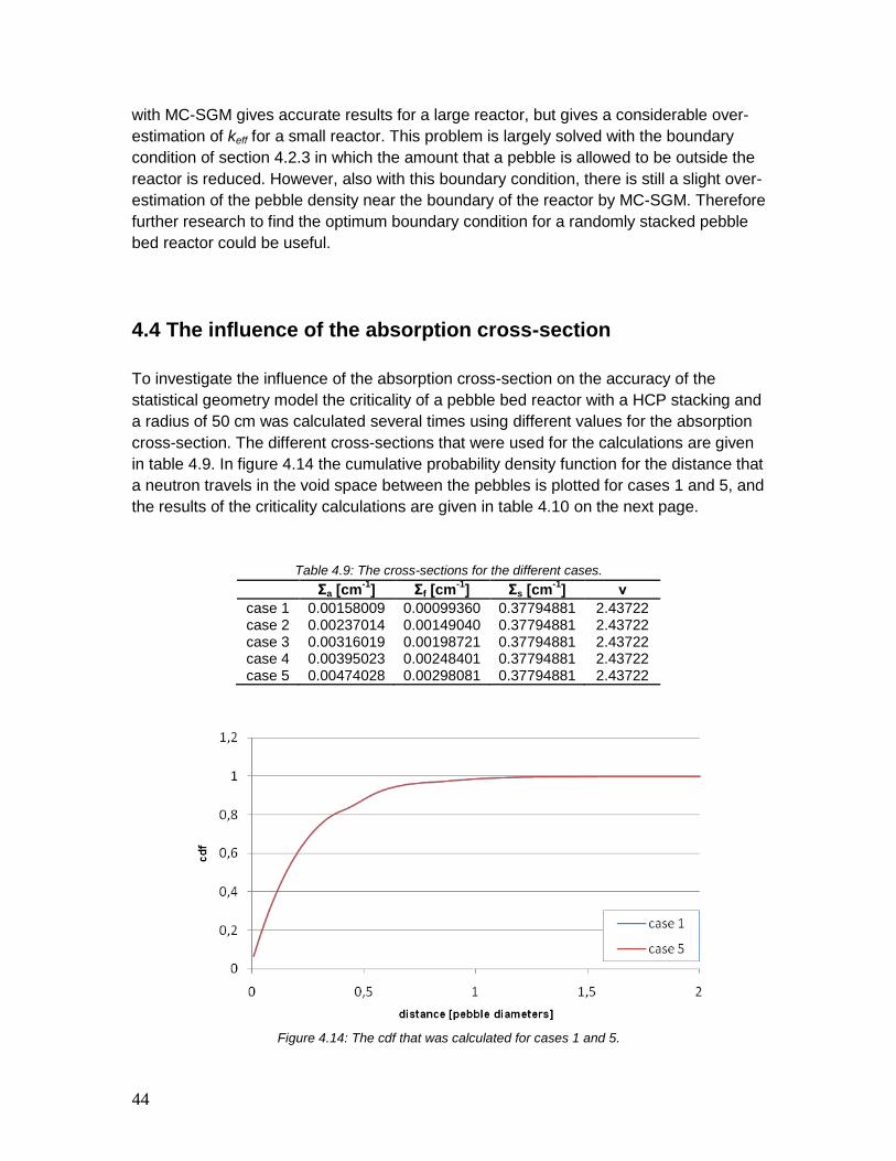
44

with MC-SGM gives accurate results for a large reactor, but gives a considerable over-

estimation of keff for a small reactor. This problem is largely solved with the boundary

condition of section 4.2.3 in which the amount that a pebble is allowed to be outside the

reactor is reduced. However, also with this boundary condition, there is still a slight over-

estimation of the pebble density near the boundary of the reactor by MC-SGM. Therefore

further research to find the optimum boundary condition for a randomly stacked pebble

bed reactor could be useful.

4.4 The influence of the absorption cross-section

To investigate the influence of the absorption cross-section on the accuracy of the

statistical geometry model the criticality of a pebble bed reactor with a HCP stacking and

a radius of 50 cm was calculated several times using different values for the absorption

cross-section. The different cross-sections that were used for the calculations are given

in table 4.9. In figure 4.14 the cumulative probability density function for the distance that

a neutron travels in the void space between the pebbles is plotted for cases 1 and 5, and

the results of the criticality calculations are given in table 4.10 on the next page.

Table 4.9: The cross-sections for the different cases.

Σa [cm-1

] Σf [cm-1

] Σs [cm-1

] ν

case 1 0.00158009 0.00099360 0.37794881 2.43722 case 2 0.00237014 0.00149040 0.37794881 2.43722 case 3 0.00316019 0.00198721 0.37794881 2.43722 case 4 0.00395023 0.00248401 0.37794881 2.43722 case 5 0.00474028 0.00298081 0.37794881 2.43722

Figure 4.14: The cdf that was calculated for cases 1 and 5.

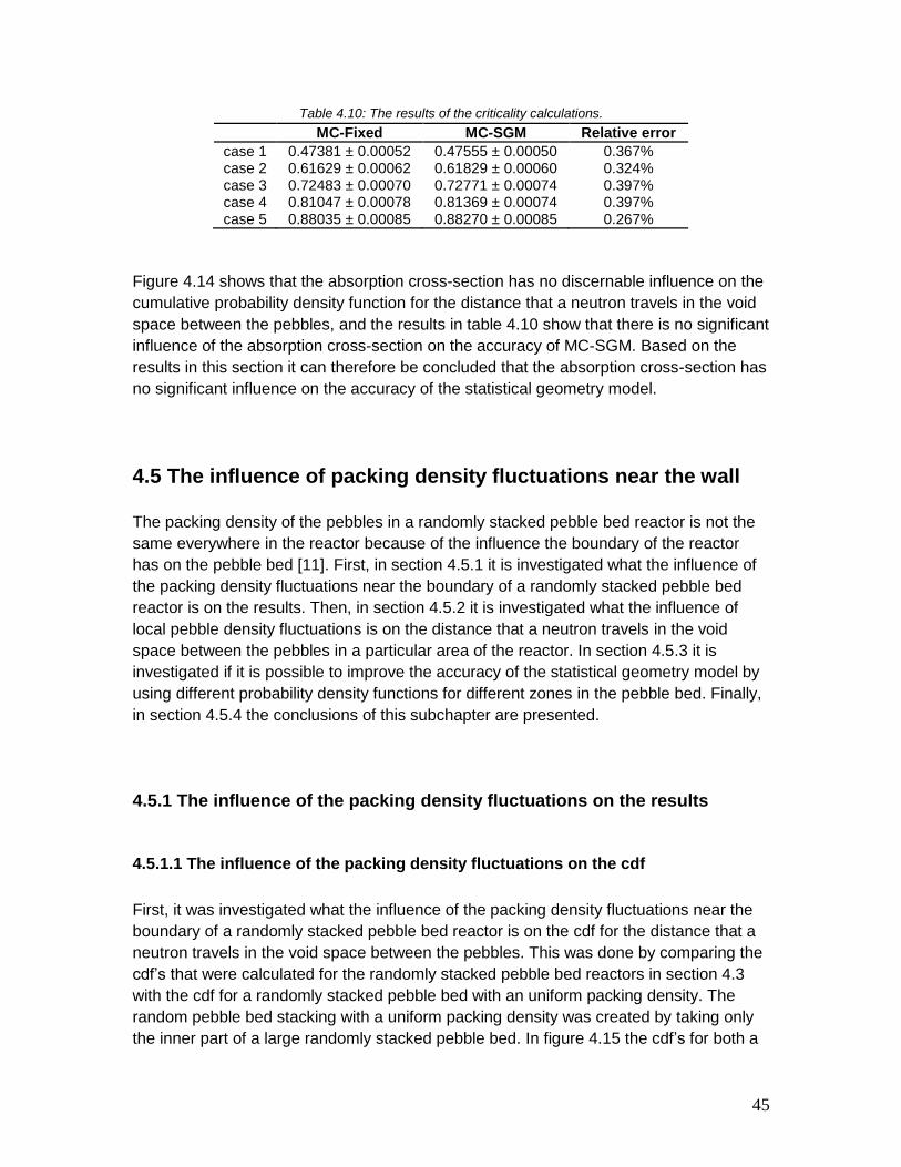
45

Table 4.10: The results of the criticality calculations.

MC-Fixed MC-SGM Relative error

case 1 0.47381 ± 0.00052 0.47555 ± 0.00050 0.367% case 2 0.61629 ± 0.00062 0.61829 ± 0.00060 0.324% case 3 0.72483 ± 0.00070 0.72771 ± 0.00074 0.397% case 4 0.81047 ± 0.00078 0.81369 ± 0.00074 0.397% case 5 0.88035 ± 0.00085 0.88270 ± 0.00085 0.267%

Figure 4.14 shows that the absorption cross-section has no discernable influence on the

cumulative probability density function for the distance that a neutron travels in the void

space between the pebbles, and the results in table 4.10 show that there is no significant

influence of the absorption cross-section on the accuracy of MC-SGM. Based on the

results in this section it can therefore be concluded that the absorption cross-section has

no significant influence on the accuracy of the statistical geometry model.

4.5 The influence of packing density fluctuations near the wall

The packing density of the pebbles in a randomly stacked pebble bed reactor is not the

same everywhere in the reactor because of the influence the boundary of the reactor

has on the pebble bed [11]. First, in section 4.5.1 it is investigated what the influence of

the packing density fluctuations near the boundary of a randomly stacked pebble bed

reactor is on the results. Then, in section 4.5.2 it is investigated what the influence of

local pebble density fluctuations is on the distance that a neutron travels in the void

space between the pebbles in a particular area of the reactor. In section 4.5.3 it is

investigated if it is possible to improve the accuracy of the statistical geometry model by

using different probability density functions for different zones in the pebble bed. Finally,

in section 4.5.4 the conclusions of this subchapter are presented.

4.5.1 The influence of the packing density fluctuations on the results

4.5.1.1 The influence of the packing density fluctuations on the cdf

First, it was investigated what the influence of the packing density fluctuations near the

boundary of a randomly stacked pebble bed reactor is on the cdf for the distance that a

neutron travels in the void space between the pebbles. This was done by comparing the

cdf’s that were calculated for the randomly stacked pebble bed reactors in section 4.3

with the cdf for a randomly stacked pebble bed with an uniform packing density. The

random pebble bed stacking with a uniform packing density was created by taking only

the inner part of a large randomly stacked pebble bed. In figure 4.15 the cdf’s for both a

46

randomly stacked pebble bed with an uniform packing density and for the randomly

stacked pebble bed reactors in section 4.3 are plotted, and in figure 4.16 the relative

difference between the cdf’s for the randomly stacked pebble bed reactors and the cdf

for the random pebble bed stacking with a uniform packing density is plotted.

Figure 4.15: The cdf for a randomly stacked pebble bed with an uniform packing density and the cdf’s for the randomly stacked pebble bed reactors .

Figure 4.16: The relative difference of the cdf’s for a randomly stacked pebble bed reactor compared to the cdf for a random stacking with a uniform packing density.

47

It can be seen in figure 4.16 that as a results of the packing density fluctuations near the

boundary of a randomly stacked pebble bed reactor, the distance that a neutron travels

in the void space between the pebbles is slightly different in a randomly stacked pebble

bed reactor compared to the distance in a random pebble bed stacking with an uniform

packing density. The distance that a neutron travels in the void space of the reactor with

a radius of 27 cm is slightly longer compared to the distance in a random stacking with a

uniform packing density, while for the other reactors the distance is slightly shorter. It can

also be seen that the influence of the packing density fluctuations becomes smaller for a

larger reactor, which is also expected since the influence of the volume close to the

boundary of the reactor on the cdf becomes smaller for a larger reactor. It can therefore

be concluded that especially for a small reactor, there is an influence of the packing

density fluctuations near the boundary of a randomly stacked pebble bed reactor on the

cumulative probability density function for the distance that a neutron travels in the void

space between the pebbles.

4.5.1.2 The influence on the results of MC-SGM

Next, it was investigated what the influence of the packing density fluctuations near the

boundary of a randomly stacked pebble bed reactor is on the results of MC-SGM. This

was done by recalculating the criticality of the randomly stacked pebble bed reactors in

section 4.3 with MC-SGM, using the cdf for a randomly stacked pebble bed with a

uniform packing density for the calculations, and comparing the results with those in

section 4.3.3. The results are given in table 4.11.

Table 4.11: The influence of the non-uniform packing density on keff

Radius of the reactor

With packing density fluctuations

Without packing density fluctuations

Relative Error

15 cm 0.10680 ± 0.00019 0.10563 ± 0.00014 -1.095% 27 cm 0.25558 ± 0.00040 0.25766 ± 0.00032 0.813% 50 cm 0.59033 ± 0.00081 0.59032 ± 0.00062 -0.001% 90 cm 1.01089 ± 0.00097 1.00972 ± 0.00100 -0.115% 120 cm 1.18419 ± 0.00150 1.18216 ± 0.00103 -0.171%

The results in table 4.11 show that for a small reactor, there is a small but significant

difference between the calculated values of keff, while for the larger reactors, the results

are in good agreement with each other. This is expected since for a small reactor, there

is a considerable influence of the packing density fluctuations on the cdf, while for a

large reactor, the influence is much smaller. It can also be seen that for the reactor with

a radius of 27 cm, there is an overestimation of keff when the cdf for a random stacking

with a uniform packing density is used, while for the other reactors, there is an under-

estimation of keff. This is also expected since the distance that a neutron travels in the

void space between the pebbles in the random stacking with an uniform packing density

48

is slightly shorter compared to the actual distance in the reactor with radius of 27 cm,

while for the other reactors the distance is slightly longer compared to the distance in the

actual reactors. It can therefore be concluded that for a small reactor, there is a small but

significant influence of the packing density fluctuations near the boundary of a randomly

stacked pebble bed reactor on the results of MC-SGM, while for a larger reactor the

influence of the packing density fluctuations on the results of MC-SGM is negligible.

4.5.2 The influence of packing density fluctuations on the local distance that the neutrons travels in the void space

In section 4.5.1.1 it was already shown that especially for a small reactor, the packing

density fluctuations near the boundary of a randomly stacked pebble bed reactor

influence the distance that a neutron travels in the void space between the pebbles. In

this section it is investigated what the influence of local pebble density fluctuations is on

the distance that a neutron travels in the void space between the pebbles in a particular

area of the reactor. This was done by calculating both the radial packing fraction of a

randomly stacked pebble bed reactor and the average distance that a neutron travels in

the void space between the pebbles when it exits a pebble in a particular area of the

reactor. The results of the calculations for a randomly stacked pebble bed reactor with a

radius of 90 cm are plotted in figure 4.17.

Figure 4.17: The radial packing fraction and the average distance that a neutron travels in the void space

between the pebbles when it exits a pebble at a particular location in the reactor.

49

Figure 4.17 shows that the packing fraction fluctuations are large near the boundary of

the reactor, and disappear at about six pebble diameters from the wall. It can also be

seen that the packing fraction starts to fluctuate again in the center of the reactor, but

this is due to the fact that the area over which the packing fraction is measured becomes

very small, therefore, the local packing fraction at a point is measured instead of an

averaged value over an area. Figure 4.17 also shows that the average distance that a

neutron travels in the void space between the pebbles when it exits a pebble in a

particular area of the reactor is fairly constant for most of the reactor. However, it can

also be seen that the packing fraction fluctuations close to the wall do have an influence

on the average distance that a neutron travels in the void space between the pebbles

when it exits a pebble in that area. The decrease of the average distance in the center of

the reactor is again caused by the fact that the area over which the measurement is

done becomes very small. It can therefore be concluded that the distance that a neutron

travels in the void space between the pebbles is not the same everywhere in the pebble

bed and depends on the location of the pebble from which the neutron exits.

4.5.3 Using different cdf’s for different zones in the pebble bed

Next, the possibility to use different probability density functions for different zones in a

randomly stacked pebble bed reactor in order to improve the accuracy of the statistical

geometry model was investigated. This was done by recalculating the criticality of the

randomly stacked pebble bed reactors in section 4.3 with MC-SGM, using different cdf´s

for different zones of the reactor, and comparing the results with those in section 4.3.3.

4.5.3.1 Choosing the different zones of the pebble bed

First, it is necessary to determine the different zones in the pebble bed. This was done

by looking at the results in section 4.5.2. It can be seen in figure 4.17 that the distance

that a neutron travels in the void space when it exits a pebble in a particular area of the

reactor is the same for most of the reactor. However, it can also be seen that when

approaching the wall, the distance first decreases, and then increases close to the

boundary of the reactor. Therefore three different zones where chosen: one large zone

for the interior of the reactor, and two cylindrical shells near the boundary of the reactor.

A schematic overview of the different zones in the pebble bed is given in figure 4.18 on

the next page.

50

zone 3

zone 2

zone 1

6 cm 2 cm

Figure 4.18: The different zones of the pebble bed reactor.

4.5.3.2 Calculating the cdf’s for the different zones of the pebble bed

The cumulative probability density function for the distance that a neutron travels in the

void space between the pebbles was calculated with MC-fixed for each zone of each of

the randomly stacked pebble bed reactors in section 4.3. In figure 4.19 the results are

given for the randomly stacked pebble bed reactor with a radius of 50 cm.

Figure 4.19: The different cdf’s for each zone of the reactor.

51

It can be seen in figure 4.19 that the distance that a neutron travels in the void space

between the pebbles in zone 3 of the pebble bed is longer than the distance in the

central zone of the reactor, while in zone 2 of the pebble bed, the distance is smaller

than in the central zone of the reactor. These results are therefore in good agreement

with the results in section 4.5.2.

4.5.3.3 The results of the criticality calculations

After the cdf’s were calculated with MC-Fixed, the criticality of the randomly stacked

pebble bed reactors in section 4.3 was recalculated with MC-SGM, using different cdf´s

for the different zones of the reactor, and the results were compared with the results in

section 4.3.3. During the criticality calculations with MC-SGM the boundary condition that

was investigated in section 4.3.3 was used. The results are given in table 4.12.

Table 4.12: A comparison of the results between 1 zone and 3 zones.

Radius of the

reactor MC-Fixed

MC-SGM

1 zone 3 zones

keff Relative

error keff

Relative error

15 cm 0.10349 ± 0.00012 0.10680 ± 0.00019 3.198% 0.10564 ± 0.00014 2.077%

27 cm 0.24984 ± 0.00030 0.25558 ± 0.00040 2.297% 0.25536 ± 0.00030 2.209% 50 cm 0.58786 ± 0.00058 0.59033 ± 0.00081 0.420% 0.59001 ± 0.00060 0.365% 90 cm 1.00991 ± 0.00061 1.01089 ± 0.00097 0.097% 1.00913 ± 0.00100 -0.077%

120 cm 1.18289 ± 0.00115 1.18419 ± 0.00150 0.109% 1.18294 ± 0.00169 0.004%

Table 4.12 shows that the use of different cdf’s for two extra zones near the boundary of

a pebble bed reactor improves the accuracy of the results for the reactor with a radius of

15 cm, while for larger reactors the improvement in accuracy was not significant. This

was expected since for a small reactor, the packing density fluctuations close to the

boundary of the reactor have a considerable influence on the results, while for a large

reactor, the influence is negligible. It can therefore be concluded that using different cdf’s

for two extra zones near the boundary of a randomly stacked pebble bed reactor does

improve the accuracy of the statistical geometry model for a small reactor; however, it

has no significant effect for a large reactor.

4.5.4 Conclusion

Based on the results in this paragraph, it can be concluded that for a small randomly

stacked pebble bed reactor, there is a small but significant influence of the packing

density fluctuations in the pebble bed near the boundary of the reactor on the results,

52

however, for a large randomly stacked pebble bed reactor, the influence on the results is

negligible. This can be explained by the fact that the influence of the volume near the

boundary of the reactor in which the packing density fluctuations occur on the results

becomes smaller for a larger reactor. The packing density fluctuations in the pebble bed

near the boundary of the reactor do influence the distance that a neutron travels in the

void space between the pebbles in that area of the pebble bed. However, using different

cdf’s for two extra zones near the boundary of a randomly stacked pebble bed reactor

improves only the accuracy for a small pebble bed reactor, and has no significant effect

on the accuracy for a large reactor.

53

Chapter 5

Conclusions and Recommendations

5.1 Conclusions

The goal of this research project was to examine the accuracy of a statistical geometry

model for the analyses of a randomly stacked pebble bed reactor, and investigate which

effects are important. The effect of three different boundary conditions on the accuracy

of the statistical geometry model was investigated. Also the influence of the absorption

cross-section and the packing density fluctuations near the boundary of the reactor as

well as the effect of using different probability density functions for two extra zones near

the boundary on the accuracy of the statistical geometry model was investigated.

Using a statistical geometry model in a Monte Carlo code for the analyses of a

randomly stacked pebble bed reactor gives reasonably good results for a small reactor

and excellent results for a larger reactor, while at the same time it significantly reduces

the computation time compared to first generating a randomly stacked pebble bed, and

then performing the calculations on this bed. The statistical geometry model is therefore

very suitable for calculating the neutronics of a randomly stacked pebble bed reactor.

If no partial pebbles are allowed to be generated at the boundary of the reactor

during a calculation using a statistical geometry model, the pebble density near the

boundary is underestimated resulting in an underestimation of keff. If partial pebbles are

allowed at the boundary, the results are good for a large reactor, but for a small reactor

the pebble density near the boundary is overestimated resulting in an overestimation of

keff. If partial pebbles are allowed at the boundary but the center of each pebble still has

to be inside the reactor, the results for a small reactor improve significantly, while for a

large reactor the results improve slightly. However, for a very small reactor, the pebble

density near the boundary of the reactor is still slightly overestimated resulting in a 3 %

overestimation of keff.

54

The absorption cross-section has no discernable influence on the accuracy of the

statistical geometry model.

The fluctuations in the packing density near the boundary locally influence the

probability density function for the distance that a neutron travels in the void space

between the pebbles. However, only for a small reactor there is a small but significant

influence of the packing density fluctuations on the accuracy of the statistical geometry

model, therefore, the use of different probability density functions for two additional

zones near the boundary only improves the accuracy for a small reactor, and has no

significant effect on the accuracy of the statistical geometry model for a large reactor.

This is due to the fact that the influence of the volume close to the boundary of the

reactor in which the fluctuations occur on the results of the calculations decreases for a

larger reactor.

5.2 Recommendations

The use of an infinite cylinder in this research instead of a finite cylinder is expected to

have no significant influence on the accuracy of the statistical geometry model. However,

further research should be performed to confirm the accuracy of the statistical geometry

model for a finite pebble bed stacking.

The pebbles were modeled as spheres made of a homogeneous mixture of

graphite and TRISO particles, however, in reality a pebble consist of a graphite matrix

containing thousands of randomly distributed TRISO particles surrounded by a 5 mm

thick graphite layer. It is expected that the composition of the pebbles has an effect on

the statistical geometry model; however, it is unknown how large this effect is. Therefore,

further research is necessary to investigate the influence of the composition of the

pebbles on the accuracy of the statistical geometry model.

The results were reasonably good for a small reactor and excellent for a larger

reactor; however, for a small reactor there was still a slight overestimation of the pebble

density near the boundary of the reactor. This indicates that the boundary condition that

was used is not entirely correct, therefore, further research to find the optimum boundary

condition for a randomly stacked pebble bed reactor could be useful.

The model that was used to examine the accuracy of the statistical geometry

model should be extended to also include the graphite reflector at the boundary of the

reactor. The graphite reflector should decrease the effect the boundary condition has on

the accuracy of the statistical geometry model; however, it is unknown how large this

effect is. Therefore, further research is necessary to investigate the influence a graphite

reflector has on the accuracy of the statistical geometry model. Another extension to the

work in this thesis would be to examine the accuracy of a statistical geometry model for

the modeling of the TRISO particles inside the fuel zone of each pebble

55

Acknowledgements

I would like to thank Gert-Jan Auwerda and Jan-Leen Kloosterman for their guidance

during this research project.

56

57

Bibliography

[1] World Nuclear Association, The Nuclear Renaissance, http://www.world-nuclear.org /info/inf104.html [2] The generation IV International Forum, http://www.gen-4.org [3] PBMR, http://www.pbmr.co.za/ [4] http://cmsprod.bgu.ac.il/Eng/engn/nuclear/research/NucEnergy/GCR.htm [5] Andrew C. Kadak. A future for nuclear energy: pebble bed reactors, Int. J. of Critical Infrastructures, Vol. 1, No. 4, pp.330-345, 2005 [6] Wikipedia, Pebble bed reactor, http://en.wikipedia.org/wiki/Pebble_bed_reactor [7] J. Eduard Hoogenboom and Stavros Christoforu, reactor Physics AP3321, Special topics part II: Monte Carlo methods for neutron transport, TU Delft, 2008 [8] G. J. Auwerda, et al., Effects of Random Pebble Distribution on the Multiplication Factor

in HTR Pebble Bed Reactors, Annals of Nuclear Energy, 37:1056-1066 (2010). [9] I. Murata, et al., New Sampling Method in Continuous Energy Monte Carlo Calculation for Pebble Bed Reactors, J. Nucl. Sci. Tech. Vol. 34, No. 8, p. 734-744, 1997

[10] Isao Murata and Hiroyuki Miyamaru, Analysis of Random-Loading HTR-PROTEUS Cores with Continuous Energy Monte Carlo Code Based on A Statistical Geometry Model, International Conference on the Physics of Reactors, Interlaken, Switzerland, September 14-19, 2008. [11] G. J. Auwerda, et al., Comparison of experiments and calculations of void fraction distributions in randomly stacked pebble beds, PHYSOR 2010, Pittsburgh, Pennsylvania, USA, may 9-14, 2010

[12] J.J. Duderstadt and L. J. Hamilton. Nuclear Reactor Analysis. John Wiley and sons, 1976

[13] Atomic Archive, http://www.atomicarchive.com/Fission/Fission1.shtml [14] Wikipedia, Nuclear binding energy, http://en.wikipedia.org/wiki/Nuclear_binding_energy [15] Forrest B. Brown, Fundamentals of Monte Carlo particle transport, LA-UR-05-4983 [16] SCALE5-1, SCALE: A Modular Code System for Performing Standardized Computer

Analysis for Licensing Evaluation. Technical Report ORNL/TM-2005/39, Version 5.1, Vols. I-III. Oak Ridge National Laboratory. Available from Radiation Safety Information Computational Center at Oak Ridge National Laboratory as CCC-732.