Monopole Impedance of Finite Ground Planes - NCJRS. Department of Justice National Institute of...

" , ,

U.S. Department of Justice

Office of Justice Programs

Natioilal/llstitlltl! (JIlllsti('£'

'. -'"

Monopole Impedance and Gain Measurements of Finite Ground Planes NIJ Report 200-87

If you have issues viewing or accessing this file contact us at NCJRS.gov.

7'"".=S==;

ABOUT THE TECHNOLOGY ASSESSMENT PROGRAM

The Technology Assessment Program is sponsored by the Office of Development, Testing, and Dissemination of the National Institute of Justice (NIl), U.S. Department of Justice. The program responds to the mandate of the Justice System Improvement Act of 1979, which created NIJ and directed it to encourage research and development to improve the criminal justice system and to disseminate the results to Federal, State, and local agencies.

The Technology Assessment Program is an applied research effort that determines the technological needs of justice system agencies, sets minimum performance standards for specific devices, tests commercially available equipment against those standards, and disseminates the standards and the test results to criminal justice agencies nationwide and internationally.

The program operates through: The Tedmology Assessement Program Advisory Council (TAP AC) consisting of nationally recognized

criminal justice practitioners from Federal, State, and local agencies, which assesses technological needs and sets priorities for research programs and items to be evaluated and tested.

The Law Enforcement Standards Laboratory (LESL) at the National Bureau of Standards, which develops voluntary national performance standards for compliance testing to ensure that individual items of equipment are suitable for use by criminal justice agencies. The standards are based upon laboratory testing and evaluation of representative samples of each item of equipment to determine the key attributes, develop test methods, and establish minimum performance requirements for each essential attribute. In addition to the highly technical standards, LESL also produces user guides that explain in nontechnical terms the capabilities of available equipment.

The Technology Assessment Program Infonnation Center (TAPIC), operated by a grantee, which supervises a national compliance testing program conducted by independent agencies. The standards developed by LESL serve as performance benchmarks against which commercial equipment is measured. The facilities, personnel, and testing capabilities of the independent laboratories are evaluated by LESL prior to testing each item of equipment, and LESL helps the Information Center staff review and analyze data. Test results are published in Consumer Product Reports designed to help justice system procurement officials make informed purchasing decisions.

Publications issued by the National Institute of Justice, including those of the Technology Assessment Program, are available from the National Criminal Justice Reference Service (NCJRS), which serves as a central information and reference source for the Nation's criminal justice community. For further information, or to register with NCJRS, write to the National Institute of Justice, National Criminal Justice Reference Service, Washington, DC 20531.

o

James K Stewart, Director National Institute of Justice

u.s. Department of Justice National Institute of Justice

in

/11'002-

Monopole Impedance and Gain Measurements of Finite Ground Planes

NIJ Report 200-87

R. G. FitzGerrell Electromagnetic Fields Division Center for Electronics and Electrical Engineering N ationaI Bureau of Standards Boulder, CO 80303

May 1989

JU~ 15 \9&9

ACQUISt,.,ONS

118002 U.S. Department of Justice National Institute of Justice

This document has been reproduced exactly as received from the person or organization originating it. Points of view or opinions stat~d in this document are those of the authors and do. not nec~ssanly represent the official position or policies of the National Inslitute of Justice.

Permission to reproduce this CQ~ material has been granted by • / Public Domaln/OJP NIJ u.s: Department of JUstlce to the National Criminal Justice Reference Service (NCJRS).

Further reproduction outside of the NCJRS system requires permission of the~owner.

u.s. DEPARTMENT OF JUSTICE National Institute of Justice

James K. Stewart, Director

The technical effort to develop this report was conducted under Interagency Agreement LEAA-J-IAA-021-3, Project No. 8601.

'. , , .

ACKNOWLEDGMENTS

This report was prepared by the Law Enforcement Standards Laboratory (LESL) of the National Bureau of Standards (NBS) under th~ direction of Marshall r. Treado, Communications Systems Program Manager, and Lawrence K. Eliason, Chief of LESL. The author appreciates the help of Ramon L. resch, NBS Electromagnetic Fields Division member, who performed all of the network analyzer measurements and assisted in the antenna impedance and gain measurement program.

l

FOREWORD

The Law Enforcement Standards Laboratory (LESL) of the National Bureau of Standards (NBS) furnishes technical support to the National Institute of Justice (NIJ) program to strengthen law enforcement and criminal justice in the United States. LESL's function is to conduct research that will assist law enforcement and criminal justice agencies in the selection and procurement of quality equipment.

LESL is: 1) Subjecting existing equipment to laboratory testing and evaluation and 2) conducting research leading to the development of several series of documents, including national voluntary equipment standards, user guides, and technical reports.

This document covers research on law enforcement equipment conducted by LESL under the sponsorship of NIJ. Additional reports as well as other documents are being issued under the LESL program in the areas of protective equipment, communications equipment, security systems, weapons, emergency equipment, investigative aids, vehicles, and clothing.

Technical comments and suggestions concerning this report are invited from all interested parties. They may be addressed to the Law Enforcement Standards Laboratory, National Bureau of Standards, Gaithersburg, MD 20899.

iii

Lester D. Shubin Program Manager for Standards National Institute of Justice

CONTENTS

Page

Foreword. . . . . . . . . . . . . . . . . . . . . . . . . . . . . . . . . . . . . . . . . . . . . . . . . . . . . . . . . . . . . . . . . . . . . . . . . . . . . iii 1. Introduction... • . . . . . . . . . . . . . . . . . . . . . . . . . . . . . . . . . . . . . . . . . . . . . . . . . . . . . . . . . . . . . . . . . . . 1 2. Model Measurements. . . . . . . . . . . . . . . . . . . . . . . . . . . . . . . . . . . . . . . . . . . . . . . . . . . . . . . . . . . . . . . 1

2.1 Model Ground Planes. . . . . . . . . . . . . . . . . . . . . . . . . . . . . . . . . . . . . . . . . . . . . . . . . . . . . . . . . . 1 2.2 Using Input Impedance to Determine Minimum Circular Ground Plane Size. . . . . . . . . . 2 2.3 Model Ground Plane Configuration and Verification............................... 14 2.4 Insertion Loss and Gain Measurements. . . . . . . . . . . . . . . . . . . . . . . . . . . . . . . . . . . . . . . . . . . 22

3. Full-Scale Ground Plane Configuration and Verification................................ 27 4. References....................................................... . . . . . . . . . . . . . . . . . 38 Appendix A - Listing of Program ZMIL 77 . . . . . . . . . . . . . . . . . . . . . . . . . . . . . . . . . . . . . . . . . . . . . . . 39 Appendix B-Listing of Program GAIN77................................................ 45

v

Figure 1.

Figure 2.

Figure 3.

Figure 4.

Figure 5. Figure 6. Figure 7. Figure 8.

Figure 9.

Figure 10.

Figure 11.

Figure 12.

Figure 13.

Figure 14. Figure 15.

Figure 16.

List of Figures

Measured and calculated input impedance versus solid disk radius for a 0.0763-m monopole at 900 MHz ..•......•..•....•........................•............ Measured and calculated input impedance versus solid disk radius for a O.0763-m monopole at 800 MHz... #I" II ........... ,. ................ " " .. " " " • " " " " " " " " " " " " " " "

Measured and calculated input impedance versus solid disk radius for a 0.0763-m monopole at 1000 MHz .•..•.......•............. , ............•.......•..... View looking down on the 0.0763-m monopole centered on the inclined solid disk. The monopole element is shown full scale in the inset contact print ....•..... View of the solid disk with eight annuli removed ............•.....•............ Underside of the disk showing instrumentation used for the measurements .•....... View of the wire disk model with 16 evenly-spaced wire radials ..............•... Measured and calculated input impedance versus wire disk radius for a O.0763-m monopole at 800 MHz ....•...............•..........•............•...•..•.. Measured and calculated input impedance versus wire disk radius for a O.0763-m monopole at 900 MHz ..••.•....••••.•...•.••.••.••..••.•••.•••••••••••••••• Measured and calculated input impedance versus wire disk radius for a 0.0763-m monopole at 1000 MHz ...•............................•..•..•..•..•..•..•.. Measured and calculated input impedance versus loaded wire disk radius for a O.0763-m monopole at 800 MHz ...........•..•.•..••.....••.•..•.....•..... Measured and calculated input impedance versus loaded wire disk radius for a O.OO763-m monopole at 900 MfIz ........•..•..•..•..•....••..•..•........•.. Measured and calculated input impedance versus loaded wire disk radius for a O.0763-m monopole at 1000 MHz .....•..•..•..•..•..........•....•.......... Attachment of the 240-0 resistor between the ground plane and the wire radials .••• View of the model ground plane with the O.424-m monopoles spaced 0.4 m apart. The 16 resistors and wire radials are evenly spaced in. the angle around. the edge of the rectangular aluminum sheet •........•.......•........•..•...... Input impedance versus frequency for the O.424-m monopole on the model ground

Page

2

3

4

5 6 6 7

8

9

10

11

12

13 14

15

plane."""" ... "" .. """""""""""""" ... "" II""."""""""".""""""""""."",, .. ,,"""",,.,,"""""" 16 Figure 17. Input impedance versus frequency for the 0.166-m monopole on the model ground

plane.""""." .. """""""""""."" .. "" .. ""."""" .. """"""""""................................................ 17 Figure 18. Input impedance versus frequency for the O.093-m monopole on the model

,grotllld plan.e" " ........ ~ ...... II. ............................................................................. 'l .. .. .. .. .. • • .. .. .. .. .. .. 18 Figure 19. Input impedance versus frequency for the O.086-m monopole on the model

ground plane ................ ,. .... " .. .. . .. .. .. .. • .. .. .. .. .. . .. .. .. .. .. .. .. .. ... .. .. .. .. .. .. .. .. .. .. . .. .. .. .. .. .. .. .. .. .. .. . .. . .. .. 19 Figure 20. Input SWR versus frequency for the O.424-m and 0.166-m monopoles on the model

ground plane •..•.. ; ..•.• ,- . . . . . . • . . . . . . . . . . • . • . . . . • • . . . . . . . • . . . . . . . . . . . . . . . . 20 Figure 21. Input SWR versus frequency for the O.093-m and O.086-m monopoles on the model

grou.p.d plane. . .• . . • . . .. . . . . . . . . •. •. . • . .• . .• . . .. • . . . . . .. . . .. . . .. • . .. . • . • . . . . 21 Figure 22. Insertion loss versus frequency for the O.424-m monor-ole at O.4-m and 0.8-m

separation distances. . . . • . . . . . . • . . . . . . . • . . . . . . . • . . . . . . . . . . . • . . . • . . . • . • . . • . • • . 22 Figure 23. Insertio.n los~ versus frequency for the O.166-m monopole at O.4-m and 0.8·m

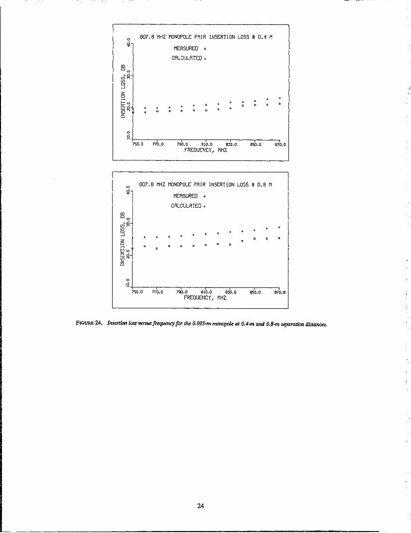
separatton distances .................................................................... ,. ... ,. .. " ... ,. .... " . 23 Figure 24. Insertion loss versus frequency for the 0.093-m monopole at O.4-m and 0.8-m

separation distances .................................................................. ,. ... ,. ... ,. ... " .... ,. .......... 1# .. 24 Figure 25. Inserti~n lo~ versus frequency for the 0.086-m monopole at O.4-m and O.8-m

separation distances ................................................................... ,. .......... 1# III .. '" .... 1# ..... " ,.,. • lit .. ... .. .. 25 Figure 26. Mismatch loss versus frequency for the 0.424-m and 0.166-m monopoles on the

model ground plan.e ....................................................... ,. .... ,. .... " .... II .. .. .. .. .. .. .. .. .. .... .. .... .. .. .. .. .. 26 Figure 27. Mismatch 1000 versus frequency for the 0.093-m and 0.086-m monopoles on the

model groun.d plane ........................... II II .. 10 ill ill II .. ,., ........ II ................... II .. .. .. .. .. .. .. • .. .. .. .. .. .. .. .. .. .. 27

vi

Page

Figure 28. Schematic of SWR measurement, above; schematic of insertion loss measurement, below II" •••••••••••••••••••••••••••••••••••• "."""""""""",,.,,"" II ""."" II" .. """". 28

Figure 29. Photograph of the full-scale test facility with 2.43-m test antennas and resistively-loaded radials ..........•..•....• , . . . . . . . . . • . . . . . . . . . . . . . . . . . . . . . . . 29

Figure 30. Full-scale SWR versus frequency for the 2.43-m monopole. . . . . . . • . . . . . . . . . . . . . . . 30 Figure 31. Full-scale insertion loss versus frequency for two identical 2.43-m monopoles

1.S m apart" II ...... , " II II • " " " " , II II II " • II II II " ,. " II " II II II II • " II II ... " II II ... II " " II " II " II II II " II " II II • II " " II 30 Figure 32. Full-scale insertion loss versus frequency for two identical 2.43-m monopoles

2mapart .................................................................. 31 Figure 33. Full-scale SWR versus frequency for the 1.72-m monopole......... ....•.. .. . .. .. 31 Figure 34. Full-scale insertion loss versus frequency for two identical1.72-m monopoles

1 m apart II II II "" II II II"" II II" II" II II II. II II II II II II """" II II." "" II II" "" II •• """ .. II II II" II """""." II II II" II'" 32 Figure 35. Full-scale insertion loss versus frequency for two identical1.72-m monopoles

1.5 m apart. . . . . . • . . • . . . . . . . . . . . . . . . . . . . . . . . . • . . . . . . . . • . . . . . . . . . . . . . . . . . . . . 32 Figure 36. Full-scale insertion loss versus frequency for two identical1.72-m

monopoles 2 m apart. . . . . . . . . . . . . . . . . . . . . . . . . . . . . . . . . . . . . . . . . . . . . . . . . . . . . . . . 33 Figure 37. Full-scale SWR versus frequency for the 0.445-m monopole. . . . . . . . . . . . . . . . • . . . . . 33 Figure 38. Full-scale insertion loss versus frequency for two identical 0.445-m monopoles

0.36 m apart. . . . . . . • . . . . . . . . . . • . . . . . . . • . . • . . . . . . . . . . . . . . . . . . . . . . . . . . . . . . . . . . 34 Figure 39. Full-scale insertion loss versus frequency for two identical 0.445-m monopoles

0.5 m apart" II " II II II II " " II II ill II II " " II II II " " • II " II II .. " • II II II II " II II " " • II .... II II " • II •• " II II II II " II " " II II II " " 34 Figure 40. Full-scale insertion loss versus frequency for two identical 0.445-m monopoles

1 m apart. " II II II II • " II II " II , II .. II " " II " .. II • II " " " " II II " II II II II II II " " • II II II II II " II II II II • II " 6 II II " II II II II " II II II • 35 Figure 41. Full-scale SWR versus frequency for the 0.156-m monopole. . . . . . . . . • . • . . . . . . . . . . 35 Figure 42. Full-scale insertion loss versus frequency for two identical 0.156-m monopoles

0.24 m apart. II II ••••••••••• II ...... fI II " " ...... II ............................... II • .. • • .. .. .. • • • • .. .. .. 36 Figure 43. Full-scale insertion loss versus frequency for two identical 0.156-m monopoles

0.36 m apart. . • . . . . . . . . . . . . . . . . . . . . . . . • . • . . . . . . . • . . . . . . . . . . . . . • . . . . . . . . . . . . 36 Figure 44. Full-scale SWR versus frequency for the 0.0845-m monopole. . . . . . • . . • . . . . . . . . . . . 37 Figure 45. Full-scale insertion loss versus frequency for two identical O.0845-m monopoles

0.12 m apart. . . . . . • . . . • . . . . . • . . . . . . . • . • . . . • • . . • . . . . . . . • . . . . . . . . • • . . . . . . . . . . 37 Figure 46. Full-scale insertion loss versus frequency for two identical 0.0845-m monopoles

0.18 m apart . . . . . . . . . . . . . . . . . . • . . . . . . . . . . . . . . . . . . . . . . . . . . • . . . . . . • . . . . . . . . . . 38

I .. r· i

vii

A ac AM cd cm CP cis d dB dc °C OF diam emf eq F fc fig. FM ft ft/s g g gr

COMMONLY USED SYMBOLS AND ABBREVIATIONS

ampere H henry nm alternating current h hour No. amplitude modulation hf high frequency o.d. candela Hz hertz (cIs) n centimeter i.d. inside diameter p. chemically pure in inch Pa cycle per second ir infrared pe day J joule pp. decibel L lambert ppm direct current L liter qt degree Celsius Ib pound rad degree Fahrenheit Ibf pound-force rf diameter Ibf·in pound-force inch rh electromotive force 1m lumen s equation In logarithm (natural) SD farad log logarithm (common) sec. footcandle M molar SWR figure m meter uhf frequency modulation min minute uv foot foot per second acceleration gram grain

mm millimeter V mph mile per hour vhf mls meter per second W N newton A N'm newton meter wt

- .t2 ( ft2' 2 ). 1 _.t;3 ( ft3 3 ) area-uw e.g., ,ID, etc. ,vo ume-uw e.g., ,m, etc.

PREFIXES

d deci (10-1) da deka (10) c centi (lQ-~ h hecto (1Q2) m milli (10-3) k kilo (1(}l) ~ micro (10-6) M mega (106) n nano (10-~ G giga (1Q9) p pico (10-12) T tera (1012)

COMMON CONVERSIONS (See ASI'M E380)

ft/s X 0.3048000= mls ft x 0.3048 = m ftolbfx 1.355818=J gr x 0.06479891:= g inx2.54=cm kWhx3600000=J

Ib x 0.4535924 = kg lbfx 4.448222 = N lbf/ftx 14.59390=N/m Ibf.in x 0.1129848 = N'm Ibf/in2x 6894.757= Pa mph x 1.609344=km/h qt x 0.9463529 = L

Temperature: (T·p - 32) x 519 = T·c

Temperature: (T·cX9/5)+32=T.p

viii

nanometer number outside diameter ohm page pascal probable error pages part per million quart radian radio frequency relative humidity second standard deviation section standing wave radio ultrahigh frequency ultraviolet volt very high frequency watt wavelength weight

l

NIJ Report 2<>0-87

MONOPOLE IMPEDANCE AND GAIN MEASUREMENTS OF FINITE GROUND PLANES

R. G. FltzGerrell*

National Bureau of Standards, Boulder, CO 80303

The purpose of the work descnbed in this report is to determine if it is possible to make acceptably accurate input impedance and gain measurements of monopoles on a reduced size ground plane. Ideally, monopoles are measured with the antenna located on an infinite, perfectly conducting, ground plane. Practically, measurements are made on a test site with dimensions largely determined by the cost and availability of the space occupied by the site. Theoretical calculations show that the radius of a highly conducting ground plane should be at least 2 A, where A = wavelength, for measuring the input impedance of 0.25 A monopoles. At 25 MHz, the lOWest frequency considered here, such a ground plane would require a space at least 48 m (157 ft) in diameter. Model impedance measurements and calculations presented in this report imply that a space on the order of 10 by 11 m (33 by 36 ft) may be sufficient if the researcher uses 16 resistively-loaded wire radials to extend a 3.66 by 4.88 m (12 by 16 ft) solid metal ground plane. Measured insertion loss data acquired using a 1:5 scale model ground plane with resistively-loaded radials indicate that this area is sufficiently large for gain measurements as well. Measured and calculated monopole SWR and insertion loss on a full-scale ground plane verify th(l results of the model measurements.

Key words: gain measurement; impedance measurement; insertion loss; monopole antenna; reduced size ground plane; standard antenna; standing wave ratio.

1. INTRODUCTION

A gain-standard antenna, or s~ply standard antenna, is one having gain-pattern and input-impedance characteristics that are known with a small degree of uncertainty. Standard antennas are typically used in gain-transfer measurements to determine the gain of test antennas by comparing the signal level received by the test antenna to that received by the struldard antenna when it replaces the test antenna [in a plane-wave field generated] on an antenna test· range. For simplicity and accuracy, the standard antenna should have polarization and gain patterns similar to those of the test antenna. Therefore, a monopole standard antenna should be used to determine the gain of a monopole test antenna if the standard's input impedance and gain are to be accurately determined.

Accurately determining gain and impedance parameters for standard monopoles ordinarily requires that they be located on an electrically large, highly conducting ground plane [1,2p. The primary contribution of this report is applying a resistive loading technique [3] to make a small ground plane appear to be electrically larger than its physical dimensions would indicate.

2. MODEL MEASUREMENTS

2.1 Model Ground Planes

Model ground planes were centered on a 2.14 m (7.02 ft) diameter foamed polystyrene disk on top of a cart, placing the feedpoints 1.6 m (5.25 ft) above ground, on the underside of the ground plane. The relative dielectric constant of the disk is 1.03 to approximate free space. All measurements were made with a computer-controlled network analyzer system located on the cart below the center of this disk, thus minimizing cable lengths between the instrumentation and the antenna feedpoints.

In this report, the uncertainty of the standard monopole input impedance was determined by comparing measured and calculated impedance data for various ground plane configurations. The uncertainty of the standard monopole gain was determined by comparing measured and calculated insertion loss data for two

• Electromagnetic Fields Division, Center for Electronics and Electrical Engineering, National Engineering Laboratory. 1 Numbers in brackets refer to references in section 4.

1

identicalwonopoles at specified separation distances on a ground plane having resistively~loaded radials and designed to satisfy the input impedance requirements. Minimizing the difference between measured and calculated input impedance was assumed to be the most stringent design criterion for the ground plane. After the ground plane configuration was determined based on impedance measurements, the insertion loss data were measured.

2.2 Using Input Impedance to Determine Minimum Circular Ground Plane Size

Input impedance of thin linear monopoles was calculated by extrapolation from the data tables in [4], supplemented by data tables calculated using equations in [5]. The input impedance of thin linear monopoles over finite ground planes was obtained from the data in [6], "for monopole antenna[s] at the center of a perfectly conducting circular disk in free space."

Figures 1, 2, and 3 show the results of the initial set of impedance versus ground plane disk radius measurements peri-:>rmed with a single, fixed length, monopole chosen to duplicate that used for Richmond's

o o ...

, ~o

Zo -",

N

...J~ 0: In w N

0::

o

8 o ,,;

U1 :E: :Co C) • o ~

z~ ...... In N'

o >-<0 g§, Zo (DtA 0:, :<..... 0

~

MONOPOLE IMPEDANCE, REAL PART @ 900 MHZ

Q Q Q Q

0.0 0.5 1.0 1.5 2.0 2.5 3.0 3.5 1.0 SOLID DISK RADIUS, WAVE LENGTH

MONOPOLE IMPEDANCE, IMAGINARY PART @ 900 MHZ

~+----r---.----~---r---.----r----.---' 0.0 0.5 1.0 1.5 2.0 2.5 3.0 3.5 1.0

SOLID DISK RADIUS, WAVE LENGTH

FIGURE 1. Measured and calculated input impedance ver.SllS solid disk radius for a O.0763-m l7IOlIOpole at 900 MHz. Calculated by Richmond -11-11-. Calculated by Jang et al. (infinite disk radius). Me~d 0 0 0 o.

2

~] I ,

0 ,n I'l

9 0 I'l

(Jl :cO I:,n ON

~

~o

Z· t::if:a

....19 0: III w-e::

0

=1 0 ,n

0.0

0

c::i ... , 0

tf')~ :C' I: 00

,~ ~ , z Nq ~1Il

III >0' e:: 0:0 zc::i -to (.!), 0: :Co - . III

to , 0

c::i r;-0.0


o g

iii i 0.5 1.0 1.5 2.0 2.5 3.0

SOLID DISK RADIUS, WAVE LENGTH

I 3.5


Q Q Q Q Q

I 4.0

0.5 1.0 1.5 2.0 2.5 3.0 3.5 4.0 SOLID DISK RADIUS, WAVE LENGTH

FIGURB 2. Measurtd and calculated input impedance versus solid disk radius for a O.0763-m 1TWtlOpOle at 800 MHz. Calculated by King et a1. (infinite disk radius). Measured 0 0 0 0 •

A ..

calculations at 900 MHz [6]. Monopole length and radius were 0.229 A (0.0763 m) and 0.003 A (0.001 m) respectively. The ground plane was a 0.18 cm thick aluminum disk having a 0.4 A (0.133 m) radius, centered on a sheet of aluminum foil lightly glued to the "free-space" disk. Input impedance was measured at 800, 900, and 1000 MHz using the following procedure. The overall diameter of the ground plane was reduced in size by removing successive rings of aluminum foil 0.2 A (0.067 m) wide until only the 0.4 A (0.133 m) radius disk remained. The measurements were made each time the annulus of foil was removed. Figures 4 and 5 show the foil covered disk at the start and midpoint of the measurement. Figure 6 shows the computer-controlled network analyzer located beneath the disk.

Excellent agreement between the data sets shown in figure 1 provides a high degree of confidence in the measured data, shown by the squares, and in the calculated data, both for an infinite radius ground plane, shown by the solid lines, and for finite radius ground planes in free space, shown by dashed lines connecting the triangles. Figures 2 and 3 show that the imaginary parts of the input impedance data do not converge to the solid lines as do those in figure 1. The measured or calculated data may not be as accurate for nonresonant monopoles as for resonant monopoles. Resonance is the frequency at which the imaginary part of the input impedance is zero for a monopole with a length near 0.25 A. For this test monopole, resonance occurs at 940 MHz.

3

0

0 "-

0

0 to

(fl :c ::c 0 0

0 ~1Jl

Z -No -0 -I"" CI: W 0:: 0

Pi 0

!<i

o (fl ,

:ctll ::c o

>-<0 0::"; CI:1"l z -C!l CI:o :c' -KJ

MO~8?OLE IMPEDANCE, REAL PART @ 1000 MHZ

o

o

o

0.0 0.5 1.0 1.5 2.0 2.5 3.0 3.5 1.0 SOLID DISK RADIUS, WAVE LENGTH


o

ODD C o

o

~~---'r----r----T'----"----,'r----r'----T'----" 0.5 1.0 1.5 2.0 2.5 3.0 3.5 4.0 0.0

SOLID DISK RADIUS, WAVE LEN~TH

FIGURE 3. Measured and calculated input impedance versus solid disk radius for a O.0763-m mu;wpcle at 1000 MHz. Calculated by King et aI. (infinite disk radius). Me~ a a a a.

4

Ul

icap Wx astt... =

FIGURE 4. Vzew looking dawn on the O.0763-m monopole centered on the inclined solid disk. The l'TIOIlOpOle dement is shown full scale in the inset contact print.

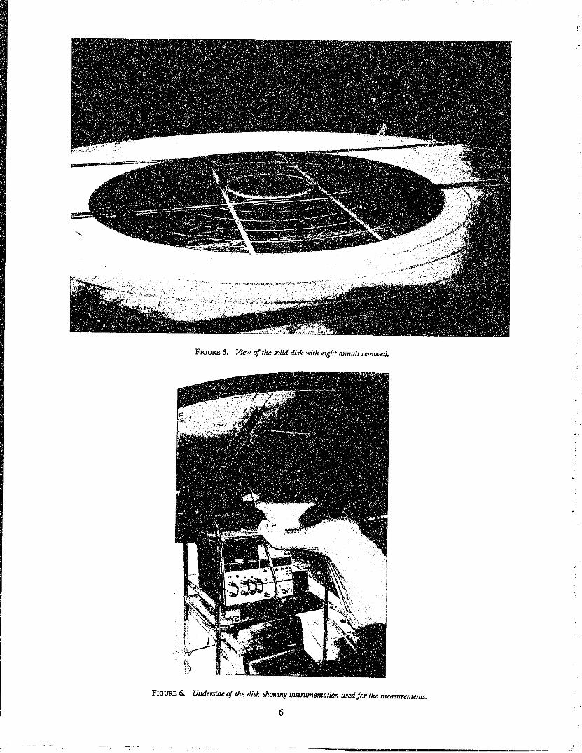
FIGURE 5. VIeW of the solid disk with eight annuli removed.

FIGURE 6. Underside of the disk showing instrumentation used for the measurements.

6

.....

The second set of measurements determined how well wire radials simulate a solid disk for impedance measurement!::. It was a duplicate of the first measurement except the aluminum foil ground plane was replaced by 16 evenly spaced #26 copper wire radials as shown in figure 7. Impedance was measured, a 0.2 >.. length was clipped from the end of each radial, and the measurements were repeated until only the 0.4 >..

, .... k

.~~~~~~ ~~!!HliiIllli\l1llJlW ,.'

FIGURE 7. VIeW of the wire disk model with 16 evenly-spaced wire radials.

radius disk remained. Figures 8, 9, and 10 differ substantially from the previous figures, and the data show no indication of convergence to the infinite radius, solid disk line. The choice of 16 radials is assumed to be a reasonable number that would be acceptable for use by industry personnel to fabricate temporary or permanent monopole test facilities.

The third set of measurements determined if Altshuler's resistively-loading technique [3] would work for this particular application. This technique alters the standing-wave current distribution on a linear wire antenna so that it is more like a traveling-wave distribution by inserting a 240-.0 resistor 0.25 >.. from the open end of the wire. The resistor tends to terminate the wire in its characteristic impedance by minimizing the wave reflected at the wire end. The result is a large traveling wave with a small, superimposed standing wave on the wire. As viewed from the monopole terminals, the ground plane with resistively-loaded radials appears to be very large.

Eleven 240-.0 resistors, with 0.2->" (0.083-m) spacings starting at the open end of the wire, were placed serially in parallel with each wire radial. The wires bridging the outermost resistors were cut away. Monopole impedance was measured, then the outermost resistors and 0.25->.. sections of the radials were cut away, the sections of wire bridging the next outermost resistors were cut away, and the measurements were repeated until only the 0.4->" radius disk remained. Figures 11, 12, and 13 show a considerable improvement in the behavior of the input impedance as a function of radial length, indicating that resistively-loaded radials do work for this particular application.

At this point, model measurements closely resembling the proposed gain and impedance measurements are performed using a resistively-loaded ground plane.

7

o ci f')

(f)

4 0

J:.n ON

-~O Z· N~

...J~ a:"' w-a::

o

"'


o

o 0

ul+-----r_---,-----.-----r�-----r�----~I----~I --~I

o ci ... , o

U1~ :1:' J: 00

~~ ~ , z N~ - "' "' :>0<' a:: a:o Zci _w c!)' a: ~~

"' w , o

0.0 0.5 1.0 1.5 2.0 2.5 3.0 3.5 4.0 WIRE DISK RADIUS, WAVE LENGTH


o

a

o 0

o

1.0 ~i_~--r----,-----.----.-----r---~-----r--~

0.0 0.5 1.0 1.5 2.0 2.5 3.0 3.5 WIRE DISK RADIUS, WAVE LENGTH

FIOURE 8. Measured and calculated input impedance venus wire disk radius for a O.0763-m monopole at 80{) MHz. Calculated by King et al. (infinite disk radius). Measured 0 0 0 Cl •

8

0 .,; ..,.

0

g (f) ~o I"; 0'"

-~O z· ~g N

...J~ a: 1J1

w N

0:: 0

0 N

0

~

o o

(f) ~ Io o . o

-zc: ~1J1

N' o

>-<0 g§I ~C? lET ~ --. 0

o ~ o


0.0 i i 0.5 1.0 1.5 2.0 2.5 3.0 3.5 4.0

WIRE DISK RADIUS, WAVE LENGTH


o 0

~+-----r----.-----r----'-----.---~r----r----~ 0.0 0.5 1.0 1.5 2.0 2.5 3.0 3.5 4.0


FIGURE 9. Measured and calculated input impedance venus wire disk radius for a O. 0763-m monopole at 900 MHz. Calculated by lUng et aI. (infinite disk radius). Measured 0 0 0 D.

9

0 MONOPOLE IMPEOANCt, REAL PART @ 1000 MHZ

0 "-

0

0 lO

(f) ::c :r: 00 a

0 ~'"

Z

No -0 -1'" cr: W 0:: 0

0 "' 0

0 N

0.0 0.5 1.0 1.5 2.0 2.5 3.0 3.5 1.0 WIRE DISK RADIUS, WAVE LENGTH

0 MONOPOLE II1PEDANCE, IMAGINARY PART @ 1000 MHZ

,n (0

a 0

(f) •

::ctll ::r: 0

~o ztn ......... a

N

)-<0 O::,n a cr:"' z ...... C!l cr:o ::c • ...... \(1

D 0

!d 0.0 0.5 1.0 1.5 2.0 2.5 3.0 3.5 4.0


F1GURB 10. Measured and calculated input impe(umce lle1'l'US wire disk radius for a O. 0763-m monopole at 1000 MHz. Calculated by King et al. (infmite disk radius). Measured 0 0 0 o.

10

0 .,; '" 0

d '"

~~ i§~ ~

-- 0 z· ...... l'<l N

--l~ a: III W-0::

0

~

0 .,;

o d ... I

o

(f)~ :C I

::c Do

,~ - I Z

NC: ~1Il

III

>-0 ' 0:: a:o Zd ...... CD (!II

a: :Co

-~ o o


a

0.0 0.5 1.0 1.5 2.0 2.5 3.0 3.5 i.O LOADED WIRE DISK RADIUS, WAVE LENGTH


a

a

0.0 ~i-----'-----.-----r-----r---___ r----'-----.----,

0.5 1.0 1.5 2.0 2.5 3.0 3.5 4.0 LOADED WIRE DISK RADIUS, WAVE LENGTH

FIGURE 11. Measured and co.lculated input impedance venus loaded wire disk radius/or a O.0763-mmonopole at 800 MHz. Calculated by King et al. (in[miJe disk radius). Measured 0 0 0 0 •

11

0

.n ....

0

ci .... U1 l::0 :C.n 0""

~O

Zci -,., N

....J"! cc'" w N

0:: 0

ci N

0

~

o

8 o .n

U1 l:: :Co o . o

Z"! -Ill NI

o

i:2s! CCI Z", C!)u1 CC, l::

-'" l'i b

0.0


o Q o

o

I i I o.S 1.0 1.S 2.0 2.5 3.0 3.S 4.0

LOADED WIRE DISK RADIUS, WAVE LENGTH


o

~4-----r----'-----r----'-----r----'-----r--~ 0.0 0.5 1.0 1.5 2.0 2.5 3.0 3.5 1.0

LOADED WIRE DISK RADIUS, WAVE LENGTH

FIGUltB 12. Measured and calculated input impedance verms loaded wire disk radius for a O. oo763-m T7lOIWpole at 900 MHz. Calculated by King et al. (inflllite disk radius). Measured 0 0 0 CJ.

12

(fl E

o d " o d to

::r: 00

d ,in

Z

o d

MONOPOL~ IMP~DANC~, R~AL PART @ 1000 MHZ

N+---~r----r----~--~----~----r---~--~

o iii to

o (fl •

Etil ::r: o

>-<0 C::1Ii 0:'" z ~

C!) 0:0 E' -\<l

0.0 0.5 1.0 1.5 2.0 2.5 3.0 3.5 1.0 LDAD~D WIR~ DISK RADIUS, WAV~ LENGTH

MONOPOL~ IMP~DANC~, IMAGINARY PART @ 1000 MHZ

a

a

o

~+----'-----r----r---~----'-----r---~--~ 0.0 0.5 1.0 1.5 2.0 2.5 3.0 3.5 1.0

LDAD~D WIR~ DISK RADIUS, WAVE LENGTH

FIGURE 13. Measured and calculated input impedance versus loaded wire disk radius for a O.0763-m monopole at 1000 MHz. Calculated by King et al. (infinite disk radius). Measured 0 0 0 D.

13

5TH

2.3 Model Grou~d Plane Configuration and Verification

Based on data in figures 11, 12, and 13, a model ground plane was fabricated assuming a 1:5 scale factor at the lowest design frequency of 30 MHz. Th~ result is an aluminum sheet 0.4 by 0.6 A (0.8 by 1.2 m) at 150 MHz with 16 240-0 resistors soldered to brass screws located at equal angular spacings around the edge of the sheet. No. 26 wire radials, equal to the monopole length, were soldered to these resistors as shown in figure 14. Table 1 lists the pertinent data for the model configuration shown in figure 15 with the 0.424 m (1.39 ft) monopoles at the 0.4 m (1.3 ft) separation distance.

Sheet Metal Screw & Solder Lug

Ground Plane

/ 44" X l"X 3,," Fir Slick

2400 1/4W Carbon Resistor

FIOURE 14. AttacJunent of the 240-0 resistor between the ground plane and the wire radials.

TABLB 1. Test frequencies and monopole dimensions for the model groulld plane.

Fuji scale Actual measured MOiWpoIe MOiWpo/e frequency, Scale frequency band, length·, radius,

MHz factor MHz m em

25-50 1:5 12S-225 b 0.424 0.118 150-174 1:5 750-870 0.093 0.118 400-512 1:1 400-S20 0.166 0.118 800-960 1:1 800-960 0.086 0.118

Resonalll frequency,

MHz

168 731 420 790

I These lengths are the geometric mCIIIIS of thc frcc-space values of >../4 for the two frequencies listed in column 1, with the sco1e factor applied. b Two monopoles would have been a better choice for this wide band. Emphasis was placed on the more difficult, lower end ()f this band.

Model ground plane performance verification consisted of measuring input impedance (derived from the reflection coefficient) of a single monopole centered on the ground plane extended with resistively-loaded wire radials equal to the monopole length. Two identical monopoles were then placed 0.4 m (1.3 ft) apart on the ground plane's longer center line, and the insertion loss (obtained directly as the magnitude of the transmission coefficient) was measured. This measurement was repeated at an 0.8 m (2.6 ft) separation distance. Below 150 MHz, the 0.4 m (1.3 ft) distance is close to the )./2rrr distance from an electrically small monopole to the boundary between its reactive near-field and far-field regions. Far-field illumination conditions normally imposed for antenna tests are not required for the insertion loss because it is based on mutual impedance calculations requiring only a sinusoidal current distribution on the antennas. Since the gain

14

\;

,. 1:

\

, .

FIGURE 15. VIeW of the model gT'OWld plane with the 0.424-m monopoles spact'd 0.4 m apart. The 16 resistors and wire radials are evenly spaced in the angle aT'OWld the edge of the rectangular aluminum sheet.

=

product of two antennas is an intrinsic part of insertion loss at far-field distances, gain of a test monopole relative to that of a standard monopole of similar length may be measured at near-field distances with an uncertainty based on the results of the insertion loss data.

Using a single monopole and loaded wire radial length for each set of measurements in a particular frequency band provides measured and calculated data indicating the bandwidth over which these measurements are valid. That is, the monopole and radials are electrically shorter below the monopole design frequency and longer above it. Measured and calculated input impedance versus frequency data are presented in figures 16 through 19. Agreement between these two sets of data is good, especially near the resonant frequency of the monopole, for all but the highest frequency band. Apparently the electrical spacing between the radials at the edge of the ground plane is too great, and reflections from the edge are occurring. This is shown in data in the next section by the cyclical variations in measured insertion loss data for this frequency band.

Voltage standing wave ratio, or SWR, is a scalar quantity related to input impedance that is commonly used to specify antenna performance. Figures 20 and 21 show SWR versus frequency, calculated using the impedance data from the preceding four figures. The agreement between measured and calculated data is quite good.

15

0 176.7 MHZ MONOPOLE IMPEDANCE:, REAL PART d ~ MEASURED

CALCULATED •

(f)o :c. :r: o 08 , -z

t:: -1~ a: 0 w'" 0:: 0

0

d I I I I I

125.0 145.0 165.0 185.0 205.0 225.0 fREOUENCY, MHZ

176.7 MHZ MONOPOLE IMPEDANCE, IMAGINARY PART

MEASURED 0 d CALCULATED • '" (f)-

:c :r: • Cl

, -0 z· N~

>-< 0:: a: zo - . (!)~ a:, :c

0

~ , 125.0 145.0 165.0 185.0 205.0 225.0

fREQUENCY, MHZ

FIGURE 16. Input imped(mce versus frequency for the O.424-m monopole on the model ground plane.

16

0

0 8

0

<.nO ::cOl :r: a ~

~O

zd ~w

N

.....J a: wo 0::' 0 ...

0

0 N

o o

<.nQJ

~~ 00

w ~

§ci N""

o >-<0 O::N a: ~o C!lo a: ::c .... 0

~

452.6 MHZ MONOPOLE IMPEDANCE, REAL PART

MEASURED

CALCULATED •

a

a

400.0 420.0 HO.O 460.0 480.0 500.0 FREOUENCY, MHZ


MEASURED CALCULATED •

520.0

o T+-------r-----_r------~------r_----_r------,

400.0 420.0 HO.O 460.0 480.0 500.0 520.0 FREOUENCY, MHZ

FIOURE 17. Input impedance venus frequency for the O.166-m monopole on the model ground plane.

17

~---

e:> d "

'" ~fJ :c o

....J cr: We:> ct:d .,.


MEASURED a

a .

CALCULATED •

e:>

g-f-------.------.------.-------.------.------. I I I i I I

e:> c::i III

z N~ -0

N

'"

750.0 770.0 790.0 810.0 830.0 850.0 870.0 fREOUENCY, MHZ


MEASURED a

CALCULATED •

Q

• a

d I+-------r------.,------.,r------r,------~,------~,

750.0 770.0 790.0 810.0 830.0 850.0 870.0

fRE~UENCY, MHZ

FIGURE 18. Input impedance venus frequency for the O.093-m monopole on the model ground plane.

18

o o ....

o

~g :c o ,

- 0 z· N~

....J a::: wo c::. o ...


MEASURED

CALCULATED A

a

a a

a

o

g.~----.-----.-----r----'r----'----~----~~--, -, , iii

o g o o

(f")111 l:: :cO 00 ... , ~~ N M

o >-<0 C::N a::: zo ...... c,!)o a:::l:: ..... 0

o o

600.0 620.0 610.0 660.0 660.0 900.0 920.0 910.0 960.0 fRE~UENCY, MHZ


MEASURED

CALCULATED • a

a

a

o i4-----~----r-----r_--_,----_,----~----_r----~

600.0 620.0 6010.0 660.0 660.0 900.0 920.0 910.0 960.0 fREDUENCY, MHZ

FIOURE 19. Input impedance venus frequency for the O.086-m mcnopoIe 011 the model ground plane.

19

0:: :;:: (J1

>

o ci" '"

o

8

o

176.7 MHZ MONOPOLE SWR

MEASURED

CALCULATED •

ci+--------r-------.-------,--------r---__ ~ 125.0 145.0 165.0 185.0 205.0 225.0

PREOUENCY, MHZ

0 452.6 MHZ MONOPOLE SWR

to MEASURED

CALCULATED •

0 .;. .

D

0

N

~

0

ci 400.0 420.0 HO.O 160.0 480.0 500.0 520.0

PREOUENCY, MHZ

FIGURE 20. Input SWR versus frequency for the 0.424-m and O.166-m monopoles 011 the model ground plane.

~ ______________ 20 _______________ __

0:: :;:: (J)

>

0:: ::;:: (J)

>

807.8 MHZ MONOPOLE SNR 0

.0 MEASURED a

CALCULATED •

~ ..,..

0

N

o ci.~ ____ -. ______ .-____ ~ ______ .-____ ~~ __ ~

750.0 770.0 790.0 810.0 830.0 850.0 870.0 FREOUENCY, MHZ

876.4 MHZ MONOPOLE SNR 0

.0 MEASURED

CALCULATED •

0 .,:

0

N

o ci+----.r----r----.----,-----r----.----.--~

800.0 820.0 840. a 860. a 880.0 900.0 920.0 940.0 960.0 FREOUENCY, MHZ

FIGURE 21. Input SWR versus frequency for the O.093-m and O.086-m monopoles on the model gT'OWld plane.

21

II

-

2.4 Insertion Loss and Gain Measurements

Substitution loss [7] is a relative measure of the transmission properties of two different waveguide junctions (two-ports or two-terminal-pair networks). It is the ratio, in decibels, of the power measured in a load with the initial two-port network in place, to the power measured in the same load with the final two-port network replacing the initial one in the transmission path. It is assumed that the generator and load characteristics remain the same for the two measurements. Insertion loss, a special case of substitution loss, is measured when the initial two-port network is perfect (a lossless, reflectionless, waveguide junction), and the reflection coefficients of the generator and load, Po and PL, are not necessarily equal to zero. The network analyzer measures the insertion loss between the terminals of two monopoles on the ground plane directly as the transmission coefficient. Initial load power is measured by the analyzer during self-calibration.

Attenuation, another special case of substitution loss, is measured when the initial two-port network is perfect and Po = PL as well. It is assumed that the difference between the transmission coefficient and attenuation is accounted for in the error budget of the network analyzer. Insertion loss data was calculated using the computer program in appendix A based on the equations in NBS Technical Note 1089 [8] assuming Po = PL, and is given as a positive number. To avoid confusion, the term insertion loss rather than attenuation is used in this document.

Figures 22-25 show measured and calculated insertion loss versus frequency for two identical monopoles at two separation distances. The effects of the ground plane edges are shown by the cyclical variation of

2ll

o o '"

CD Do

'0 tnN tn o ...J

.Z o -. f-<c ~. wo u., -Z -.

o

176.7 MHZ MONOPOLE PAIR INSERTION LOSS ~ 0.4 M

MEASURED a

CALCULATED •

a

a

o+-----~r-·----~I------'I--·-----rl ------.1 125.0 115.0 165.0 18~.0 205.0 225.0

FREOUENCY, MHZ

0 176.7 MHZ MONOPOLE PAIR INSERTION LOSS ~ 0.8 M

0 ,., MEASURED a

CALCULATED • CD Do

a a

'0 tnN a tn 0 ...J a Z 0 • f-<e ~. We tn-Z

e 0 1 1 1 1

125.0 115.0 165.0 185.0 205.0 225.0 FREOUENCY, MHZ

FIOURE 22. Insertion loss versus frequency for the O.424-m monopole at O.4-m and O.8-m separation distances.

22

[D Cl o ~O

(f")N (f") Cl ..J

Z Cl ~

~~ W O (f")-

Z

452.6 MHZ MONOPOLE PAIR INSERTION LOSS @ 0.4 M

MEASURED a

CALCULATED •

a

a

o

o+-----.------.-----r-----.----~----~ 400.0 420.0 HO.O 460.0 480.0 500.0

fREDUENCY, MHZ


MEASURED a

CALCULATED •

. a

520.0

o

o+-----.------.-----r-----.----~----~ 400.0 120.0 HO.O 460.0 480.0 500.0 520.0

fREDUENCY, MHZ

FIGURE 23. Insertion loss versus frequency for the 0.166-m monopole at O.4-m and 0.8-m separaticn distances.

insertion loss with frequency that is most apparent at the two higher frequency bands. Generally, the 0.4 m (1.3 ft) separation distance results in a smaller difference between measured and calculated data. Note that insertion loss includes mismatch losses at the monopole terminals as well as the path loss between the monopoles. One-half of the difference between the measured and calculated data is a good estimate of the accuracy of realized g&.ln. of one of the identical monopoles assuming the ground plane is perfect. Realized gain is "The power gain of an antenna in its environment, reduced by the losses due to the mismatch of the antenna input impedance to a specified impedance" [9]. A 50-n specified impedance is assumed for all measured and calculated data in this docUlllent.

23

o c::i ...

OJ Cl

0

~c::i (f)'" (f) Cl ....J

Z Cl ~

f-<o 0:: • w o (f)N

Z

o


MEASURED 0

CALCULATED 4

• a

0 Q

~4-------r------r------.-------r------r------' 750.0 770.0

OJ Cl o

~c::i (f)'" (f) Cl ....J

Z Cl -f-<o 0::. W O (f)N

Z

790.0 810.0 830.0 850.0 FREOUENCY, MHZ


MEASURED a

CALCULATED •

Q Q 0

870.0

o

~4-------r------r------.-------r------r------. 750.0 770.0 790.0 810.0 830.0 850.0 870.0

FREOUENCY, MHZ

FIGURE 24. Insertion loss vemlS frequency for the O.093-m monopole at O.4-m and O.8-m separation distances.

24

e c:i ...

co Cl e

~c:i (I'll"> (I'l o -l

Z o -~~ ~~ z


MEASURED a

CALCULATED A

• a a A ~ a A A a a

A a a a a

a A • a A •

a a a

e

8+----r--~----._--_r--_.----._--_r--_.

e ci ...

CD Cl e

~c:i (I'll"> (I'l 0 -l

Z 0 .-E-<e 0:: • We (I'lN

Z -e

8

800.0 820.0 810.0 860.0 880.0 900.0 920.0 940.0 960.0

FREOUENCY, MHZ


MEASURED a

CALCULATED A

. • A a a A . • A .

a

a a a a a a

a a

800.0 820.0 810.0 860.0 880.0 900.0 920.0 910.0 960.0

FREDUENCY, MHZ

FIOURE 25. Insertion loss ~'ersusfrequency for the O.086-m monopole at O.4-m and O.8-m separation distances.

Realized gains for the model monopoles are presented in table 2. They were calculated using computer program GAIN77 in appendix B based on equations in NBS Technical Note 1098 [10]. Mismatch losses were subtracted from the power gains to obtain the realized gains. Mismatch losses versus frequency, calculated using the SWR data in figures 20 and 21, are presented in figures 26 and 27.

As can be seen in table 2, the realized gains of these monopoles are only slightly below the theoretical 4.79-dB value for a very thin O.2S-A monopole. The mismatch losses shown in figures 26 ::md 27 tend to be minimum near the resonant frequencies of the monopoles. Fixed frequency monopoles are usually adjusted in length to minimize this mismatch loss, although the gain changes only slightly when the length is adjusted.

Full scale frequency,

MHz

35 161 452.6 876.4

Scale factor

1:5 1:5 1:1 1:1

• All monopole radii are 0.118 em.

TABLE 2. Calculated realized gains for the model monopoles'.

Frequency used for gain calculation,

MHz

176.7 807.8 452.6 876.4

25

Monopole length,

m

0.424 0.093 0.166 0.086

Gain relati~ to isotropic,

dB

4.54 4.21 4.36 4.15

'" en-

o

176.7 MHZ MONOPOLE MISMRTCH LOSS

MEASURED

CRLCULRTED •

Q

•

o+-----__ ~--__ ---r--~--~--------~----~

o M

CD Cl o

_N (11 (11 Cl ..J

:r: ~ 0:0 ;r:. (11-.... ;r:

125.0 145.0 165.0 185.0 205.0 fREOUENCY, MHZ

452.6 MHZ MONOPOLE MISMRTCH LOSS

MEASURED

CRLCULATED •

. Q

225.0

'" d+-____ -. __ ~6~_T6------._----~------._----~ 400.0 420.0 '1'10.0 460.0 480.0 500.0 520.0

fRE~UENCY, MHZ

FIGURE 26. Mismatch less versus frequency for the 0.424-m and O.166-m monopoles on the model ground plane.

26

(;)

..;

CD Cl o ~N

Ul Ul Cl ...J

:c U f-' CI:o ~-! ~

:c

o

807. 8 ~IHZ MONOPOLE M [SMATCH LOSS

MEASURED c

CALCULATED •

0+-____ .-____ .-____ .-____ .-____ .-__ -.

o ..;

CD ClCJ ~N

Ul Ul o • .J

:c u f-' CI:o :C. Ul~ ~

:c

750.0 770.0 790.0 810.0 830.0 850.0 PREOUENCY, MHZ

876.4 MHZ MONOPOLE MISMATCH LOSS

MEASURED c

CALCULATED •

c •

c • •

870.0

800.0 820.0 840.0 860.0 880.0 900.0 920.0 940.0 960.0

PREOUENCY, MHZ

FIGURE 27. Mismatch lass vernIS frequency for the O.093-m and O.086-m morwpoles on the model ground plane.

3. FULL-SCALE GROUND PLANE CONFIGURATION AND VERIFICATION

A 3.66 by 4.88 m (12 by 16 ft) wall-mounted microwave passive repeater forms the ground plane of the full-scale test facility. It is mounted horizontally with the attaching brackets supplied by the manufacturer. The height between the ground and the under surface of the ground plane and the feedpoints of the test antennas is 2.15 m (about 7 ft). This structure is designed to withstand 125 mph winds, and the surface flatness "Under no load ... will be plus 0" and minus 1/8" where negative values indicate a concave surface," as sper.ified by the manufacturer. A series of mounting holes for Type N panel jacks is located on a diagonal axis of the aluminum surface to allow insertion loss measurements at monopole-to-monopole separation distances of 0.06, 0.12, 0.18, 0.24, 0.36, 0.5, 1, 1.5, and 2 m. Sixteen resistively-loaded radials, having lengths equal to the monopole lengths, extend the electrical size of the ground plane at the frequencies below 175 MHz as dic;cussed in section 2 of this document.

27

A computer-controlled network analyzer was used for all SWR and insertion loss measurements. Antenna SWR was measured with the test monopole mounted on the panel jack nearest the center of the ground plane. Figure 28 is a schematic representation of the ground plane and the test equipment is used for the full-scale measurements. Figure 29 is a photograph of the test facility with the 2.43 m (8 ft) monopoles and radials installed. White dielectric feedpoint assemblies may be seen in this photograph. They are used with the test antennas in the two lower frequency bands for mechanical support.

Resistively Loaded RadialS

I 1/ Test Antenna

-* Metal I r Ground Plane ---J

Network Analyzer

Network Analyzer

FIGURE 28. Schematic of SWR measurement, above; schematic of insertion loss measurement, below.

28

FIGURE 29. Photograph of the full-scale test facility with 2.43-m test antennas and resistively-loaded radials.

The characteristics of the monopole test antennas used for the full-scale measurements are given in table 3. These antennas are the gain-standard monopoles proposed for the NIJ Standard for Mobile Antennas [11].

TABLB 3. Test frequencies and monopole dimensions for the full-scale ground plane.

Frequency Base TIp Resonant band, Length, radius, radius, frequency,

MHz m c em MHz

25-35 2.43 0.5 0.125 29.65 35-50 1.72 0.5 0.27 41.5

150-174 0.445 0.24 0.24 157.5 400-510 0.156 0.24 0.24 435 805-865 0.0845 0.24 0.24 775

Full-scale SWR and insertion loss data are presented in figures 30-46. The difference between measured and calculated data gives a reasonable estimate of measurement uncertainty using the finite ground plane. SWR uncertainty is estimated to be the difference between the measured and calculated data. Uncertainty in monopole gain is estimated to be one-half the difference between the measured and calculated insertion loss data curves because the gain product of an identical monopole pair is an intrinsic part of the insertion loss. Measured data most closely matches the calculated data at the resonant frequencies of the monopoles, as it did for the model measurements.

The full-scale ground plane is large enough for measurements in the two highest frequency bands without resistively-loaded radials. None of the full-scale measurements show cyclical variations with frequency that would indicate reflections from the edges of the ground plane or a nearby building.

29

o

2.43 M MONOPOLE SWR

~lEASURED

CALCULATED •

o_~--------------------r---------------------' 25.0 30.0

FREOUENCY, MHZ 35.0

FWURE 30. FuJI-scale SWR versus frequency for the 2.43-m monopole.

2.43 M MONOPOLE INSERTION LOSS @ 1. 5 M 0

0 n MEASURED

CALCULATED • CD 0

0

-0 lflN In 0 -I

Z 0

t-o • 0:: • w o lfl-

~

0

0 25.0 30.0 35.0

FREOUENCY, MHZ

FIGURE 31. Full-scale insertion loss versus frequency for tiro identical 2.43-m monopoles 13 m apart.

30

I

- ---"

2.43 M MONOPOLE INSERTION LOSS @ 2.0 M e 0 I'l MEASURE;U

CALCULATED A

en Cl

0

-0 tnN tn Cl ..J

Z 0 - c 1-'0 0:: • We A tn- • Z -

e 0

25.0 30.0 35.0 fREOUENCY, MHZ

FIGURE 32. Fuji-scale insertion loss versus frequency for too idrmticaI2.43-m monopoles 2 m apart.

1.72 M MONOPOLE SHR 0

~ MEASURED

~ CALCULATED A

I 0

g

0:: ::;:: tn

0

iii

"! o+--------------r--------------.-__________ ~ 3~.0 10.0 45.0 50.0

fRE~UENCY, MHZ

FIGURE 33. Fuji-scale SWR versus frequency for the 1. 72-m monopole.

31

----, ----.... -------------------..:..----------.:.....----.1

tIl 0

0

'0 lflN lfl o -l •

Z • o

~~ we lfl-Z -

o

1.72 M MONOPOLE INSERTION LOSS @ 1 M

•


• • • . • •

•

04--------------.--------------r-------------~ 35.0 10.0 45.0 50.0

fREOUENCY, MHZ

FIGURE 34. Fuji-scale insertion loss venus frequency for hID identical 1. 72-m monopoles 1 m apart.

tIl o

e o 1'1

e '0

lfl'" lfl o -l

Z o

~~ we lflZ

e

•

1.72 M MONOPOLE INSERTION LOSS @ 1.5 M

MEASURED

CALCULATED •

• . . • . . •

. •

o+--------------.--------------r-----______ ~ 35.0 10.0 45.0 50.0

fRE~UENCY, MHZ

FIGURE 35. FuJl-scale insertion loss versus frequency for hID identical 1. 72-m monopoles 1.5 m apart.

32

1

OJ

°0 '0

lfl'" lfl Cl ..J

Z Cl -1-<0 0::. w o lfl-Z -

o

1.72 M MONOPOLE INSERTION LOSS @ 2 M

MEASURED • CALCULATED A

•

o+-~-----------.--------------r-------------, 50:0 35.0 '10.0 '15.0

fREOUENCY, MHZ

FIGURE 36. Full-scale insertion loss versus frequency for two identicall. 72-m monopoles 2 m apart.

0

iii

~ ...

0

r-i 0:: :s:: lfl

0

N

~

0

0 150.0 155.0

0.445 M MONOPOLE SHR

MEASURED

CALCULATED A

•

160.0 165.0 fREOUENCY, MHZ

170.0 175.0

FIGURE 37. Full-scale SWR versus frequency for the O.445-m monopole.

33

-

m:1 Q ~i ~ .

t.n t.n Q -10

z~ Q

(-. 0:: W

~~ _ III

o


MEASURED •

CALCULATED •

o+--------.-------.-------.r-------r---__ ~ 150.0 155.0 160.0 165.0 170.0 175.0

FREOUENCY, MHZ

FIGURE 38. Full-scale illSertion loss versus frequency for tlW identical 0,445-m nwnopoles 0.36 m apart.

o o N

o co . Q~ ,

t.n <f) Q -10

ZS! Cl

(-.

eJ t.no z· _Ill

o

0.445 M MONOPOLE INSERTION LOSS @ O.S M

A .

MEASURED • CALCULATED •

• A o •

A

• A

• • •

o+--------.-------,-------,'--------r' -------" 150.0 155.0 150.0 155.0 110.0 175.0

FREOUENCY, MHZ

FIGURE 39. Full-scale insertion 10ss lIersusfrequency for tlW identical 0,445-m monopoles 0.5 m apart.

34

r " I

e co' o~ ,

If") If") o -Ie

zs! o Ia:: W If")e z· _ttl

=w _

0.445 M MONOPOLE INSERTION LOSS @ I M

• . MEASURED

CALCULATED •

• • . •

e

o+--------r--------.--------r-------,,-------. 150.0 155.0 160.0 165.0 170.0 175.3

FREOUENCY, MHZ

FIGURE 40. FuJI-scale insertion loss versus frequency for Pro identical 0.445-m monopoles 1 m apart.

FIGURE 41. FuJI-scale SWR versus frequency for the O.156-m monopole.

35

7& --'

o CD • Cl~ ,

Ul Ul Cl ...Jo

zs! Cl

I-< es \Q"l _11l


. •


!

•

o

o+-------r------r------,------.r------r------.

L

______ 40_0_.0 ____ 4_20_.0 _____ 4_40_._0 _____ 46_0_.0 _____ 46_0_.0 _____ 5_00_._0 520.0 \ fREOUENCY, MHZ ~

FIGURE 42. Full-scale insertion loss versus frequency for tIw identical 0.156-m monopoles 0.24 m apart.

o CD • Cl~ ,

Ul Ul o ...Jo

z~ o I-< 0:: W Ul o z· _11l



• •

o

o+-------r------r------,------.r------r------. 400.0 120.0 140.0 460.0 480.0 500.0 520.0

FREDUENCY, MHZ

FIGURE 43. Full-scale insertion loss versus frequency for t1W identical 0.156-m monopoles 0.36 m apart.

36

1

L-____ ~ ________________________ ~ ______________________________ ~ _______________________________________________________ -41

I

0 In

~ ...

0

'" a::: 3: IJ1

0

N

~

0

c:i 800.0

. •

0.0845 M MONOPOLE SWR


• .

I 825.0 850.0

fREOUENCY, MHZ

. .

I 875.0

FIGURE 44. FujI-scale SWR versus frequency for the 0.OB45-m monopole.

o co • CJ~ ~

IJ1 IJ1 CJ .....10

zB o f-a::: w 1J1 0 z· _In

~


•

MEASURED

CALCULATED •

. . . •

. •

0+-____________ ,-____________ ,-__________ --. 800.0 825.0 850.0 875.0

FRE~UENCY, MHZ

FIGURE 45. FujI-scale insertion loss versus frequency for om identical 0.OB45-m monopoles 0.12 m apart.

37

o CD • o!!! ,

til til o -10

z8 Cl

f-a:: w til 0 z . -'"

o

0.0845 M MONOPOLE INSERTION LOSS ~ 0.18 M

• • •

MEASURED •

CALCULATED •

• • • . . .

0+-________ -,,-________ -. ________ --. 800.0 825.0 850.0 875.0

PREOUENCY, MHZ

NOURB 40. P°ull-scale insertion loss versus frequency for M:> identical 0.0845-m monopoles 0.18 m apart.

4. REFERENCES

ITT =P-_

[1] FitzGerrell, R. G. Limitations on vertically polarized ground-based antennas as gain standards. IEEE T-AP-23; 1975 March: 284-286.

[2] FitzGerreIl, R. G. Standard linear antennas, 30 MHz to 1000 MHz. IEEE T-AP-34; To be published December 1986.

[3] Altshuler, E. E. The traveling-wave linear antenna. IEEE T-AP-9; 1961 July: 324-329. [4] King, R. W. P, E. A. Aronson, and C. W. Harrison, Jr. Determination of the admittance and effective

length of cylindrical antennas. Radio Science Vol. 1 (new series); 1966 July: 835-850. [5] Ma, M. T. Theory and application of antenna arrays. New York, NY: John Wiley & Sons; 1974. [6] Richmond, J. H. Monopole antenna on circular disk. IEEE-T-AP-32; 1984 December: 1282-1287. [7] Beatty, R. W. Insertion loss concepts. Proc. IEEE-52. June 1964: 663-671. [8] FitzGerrell, R. G. Site attenuation. Nat!. Bur. Stand. (U.S.) Technical Note 1089; 1985 November.

Available from the U.S. Government Printing Office, Washington, DC. [9] IEEE l$tandard definitions of terms for antennas. IEEE-T-AP-22; 1974 January: 152

[10] FitzGerrell, R. G. Linear gain-standard antennas below 1000 MHz. Nat!. Bur. Stand. (U.S.) Technical Note 1098; May 1986. Available from the U.S. Government Printing Office, Washington, DC.

[11] Mobile antennas. NIJ Standard-0205.01. National Institute of Justice, U.S. Department of Justice, Washington, DC 20531; to be published.

38

Appendix A-Listing of Program ZMIL77

00100 PROGRAM ZMIL34(INPUT,OUTPUT) 00110C*************************************************** 00120C* THIS PROGRAM CALCULATES INSERTION LOSS BETWEEN * 00130C* IDENTICAL MONOPOLES ON PLANE PERFECT GROUND. * 00135C* IT IS A MODIFICATION OF A MORE GENERAL PROGRAM * 00136C* AND SOME VARIABLES AND LINES OF CODE ARE * 00137C* REDUNDANT. * 00140C*************************************************** 00150 REAL IB,LP,LS,LAMBDA 00160 COMPLEX J,Z12B,Z12L,ZP,ZR,ZS 00170 10 FORMAT(F12.4) 00180 15 FORMAT(2F12.4) 00190 16 CONTINUE 00200 17 FORMAT(I5) 00210 18 FORMAT(*INPUT DATA AFTER EACH 7*) 00220 PRINT 18 00230 1=1 002 LI0 POLAR=O 00250 30 FORMAT(*FREQUENCY, MHZ*) 00260 PRINT 30 00270 READ 10,FREQ 00280 40 FORMAT(*ANTENNA SEPARATION DISTANCE MEASURED HORIZONTALLY, M*) 00290 PRINT 40 00300 READ 10,RS 00310 45 FORMAT(*MONOPOLE LENGTH, M*) 00320 PRINT 45 00330 READ 10,LP 00340 50 FORMAT(*MONOPOLE RADIUS, M*) 00350 PRINT 50 00360 READ 10,RADIUS 00370 RRB=RADIUS 00380 RRT=RADIUS 00390 RECZ=50. 00400 HPS=O 00410 LS=LP 00420 RSB=RADIUS 00430 RST=RADIUS 00440 SSZ=50. 00450 H2=0. 00460 IF(RSB.EQ.O) RSB=1.E-30 00470 IF(RST.EQ.O) RST=1.E-30 00480 IF(RRB.EQ.O) RRB=1.E-30 00490 IF(RRT.EQ.O) RRT=1.E-30 00500 J=CMPLX(0.,1.) 00510 PI=3.14159265 00520 LAMBDA=299.792458/FREQ 00530 BETA=2.*PI/LAMBDA

39

M*n

00540C*********************************************I*1**1******1 00550C* ALL INPUT AND MUTUAL IMPEDANCES ARE REFERRED TO THE I 00560C* BASE OR TERMINAL CURRENT. * 00570C*****************************************************1*1** 00580 100 FORMAT(*INPUT ZIN, R+JX*) 00590 PRINT 100 00600 READ 10,ZS 006l0C********************************************************1*** 00620C* PINC IS THE INITIAL LOAD POWER FROM A SSZ-OHM GENERATOR * 00630C************************************************************ 00640 PINC = 1.0 00650 PTR = PINCI(1 .-(CABS«ZS-SSZ)/(ZS+SSZ)))**2) 00660 IB = SQRT(PTR/REAL(ZS)) 00670 150 CALL ZZ(BETA,HPS,H2,J,LP,LS,LAMBDA,RS,Z12B,Z12L,POLAR) 00680 Z12B=Z12B/2. 00690 Z12L=Z12L/2. 00700 VOC=CABS(IB*Z12B) 00710 E=VOC/«LAMBDA/PI)*TAN(BETA*LP/2.)) 00720 ZP=ZS 00730 PREC=«VOC/CABS(RECZ+ZP))**2)*RECZ 00740 SLOSS=10.*ALOG10CPINC/PREC) 00750C********************************************************** 00760c* PREC IS THE FINAL LOAD POWER MEASURED USING A RECZ-OHM* 00770C* RECEIVER. SLOSS IS THE INSERTION LOSS. * 00780C********************************************************** 00790 250 FORMAT(III) 00800 PRINT 250 00810 300 FORMAT(*FREQUENCY IS *F6.1* MHZ*) 00820 PRINT 300,FREQ 00830 550 FORMAT(*WITH AN INPUT IMPEDANCE OF*F10.2*+J[*F8.2*] OHMS*) 00840 610 FORMATC*ANTENNAS ARE MONOPOLES*F6.2* M APART*) 00850 IF(HPS.EQ.O) PRINT 610,RS 00860 PRINT 550,ZP 00870 650 FORMAT(*MUTUAL IMPEDANCE IS*F10.3*+J[*F10.3*] OHMS*) 00880 651 FORMAT(*REFERRED TO THE BASE AND*) 00890 652 FORMATC*REFERRED TO THE CURRENT LOOP*) 00900 PRINT 650,Z12B 00910 PRINT 651 00920 PRINT 650,Z12L 00930 PRINT 652 00940 700 FORMAT(*INSERTION LOSS IS* F8.2* DB*) 00950 PRINT 700,SLOSS 00960 PRINT 250 00970 750 FORMATC*NEW DISTANCE OR 0 TO STOP*) 00980 PRINT 750 00990 READ 10,RS 01000 IF(RS.GT.O) GO TO 150 01010 GO TO 1000 01020 1000 CONTINUE 01030 END

40

--

01040C******************************************************************* 01050 SUBROUTINE ZZ(BETA,HPS,HS,J,LP,LS,LAMBDA,RS,Z12B,Z12L,POLAR) 01060c* COMPUTES THE MUTUAL IMPEDANCE BETWEEN IDENTICAL MONOPOLES. * 01100C******************************************************************* 01110 DIMENSION AnG(18),SI(18),CI(18),CIN(18),SIS(18), 01120+ SIL( 18) ,CIS( 18) ,CIL( 18) 01130 REAL L,LP,LS,LAMBDA 01140 COMPLEX J,Z12L,Z12B 01150 B=BETA 01160 M=O 01170 10 HP=HPS 01180 IF(POLAR.EQ.O.) D=RS 01190 IF(POLAR.EQ.l.AND.M.EQ.O.) D=SQRT(RS*RS+(HS-HP)**2) 01200 IF(POLAR.EQ.l .AND.M.EQ.l.) D=SQRT(RS*RS+(HS+HP)**2) 01210 IF(POLAR.EQ.O.AND.M.EQ.O.) H=HS-HP-LS 01220 IF(POLAR.EQ.l.) H=-LS 01230 IF(POLAR.EQ.O.AND.M.EQ.l.) H=HS+HP-LS 01240 ARG(1)=B*(SQRT(D*D+(H-LP)**2)+(H-LP» 01250 ARG(2)=B*(SQRT(D*D+(H-LP)**2)-(H-LP» 01260 ARG(3)=B*(SQRT(D*D+(H+LP)**2)-(H+LP» 01270 ARG(4)=B*(SQRT(D*D+(H+LP)**2)+(H+LP» 01280 ARG(5)=B*(SQRT(D*D+(H-LP+LS)**2)+(H-LP+LS» 01290 ARG(6)=B*(SQRT(D*D+(H-LP+LS)**2)-(H-LP+LS» 01300 ARG(7)=B*(SQRT(D*D+(H+LP+LS)**2)-~H+LP+LS» 01310 ARG(8)=B*(SQRT(D*D+(H+LP+LS)**2)+(H+LP+LS» 01320 ARG(9)=B*{SQRT(D*D+(H-LP+2.*LS)**2)+(H-LP+2.*LS» 01330 ARG(10)=B*(SQRT(D*D+(H-LP+2.*LS)**2)-(H-LP+2.*LS» 01340 ARG(11)=B*(SQRT(D*D+(H+LP+2.*LS)**2)-(H+LP+2.*LS» 01350 ARG(12)=B*(SQRT(D*D+(H+LP+2.*LS)**2)+(H+LP+2.*LS» 01360 ARG(13)=B*(SQRT(D*D+H*H)-H) 01370 ARG(14)=B*(SQRT(D*D+H*H)+H) 01380 ARG(15)=B*(SQRT(D*D+(H+LS)**2)-(H+LS» 01390 ARG(16)=B*(SQRT(D*D+(H+LS)**2)+(H+LS» 01400 ARG(17)=B*(SQRT(D*D+(H+2.*LS)**2)-(H+2.*LS» 01410 ARG(18)=B*(SQRT(D*D+(H+2.*LS)**2)+(H+2.*LS» 01420 DO 100 1=1,18 01430 100 CALL SCI(ARG(I),SI(I),CI(I),CIN(I» 01440C************************************************************* 01450C* COMPUTE MUTUAL IMPEDANCE USING EQUATIONS FROM H.E. KING * 01460c************************************************************* 01470 R12=15.*(COS(B*(LP-H»*(CI(1)+CI(2)-CI(5)-CI(6»+SIN(B*(LP-H» 01480+*(-SI(1)+SI(2)+SI(5)-SI(6»+COS(B*(LP+H»*(CI(3)+CI(4)-CI(7)-CI(8» 01490++SIN(B*(LP+H»*(-SI(3)+SI(4)+SI(7)-SI(8»+COS(B*(LP-2.*LS-H»* 01500+(-CI(5)-CI(6)+CI(9)+CI(10)+SIN(B*(LP-2.*LS-H»*(SI(5)-SI(6)-SI(9) 01510++SI(10»+COS(B*(LP+2.*LS+H»*(-CI(7)-CI(8)+CI(11)+CI(12»+SIN(B* 01520+(LP+2.*LS+H»*(SI(7)-SI(8)-SI(11)+SI(12»+2.*COS(B*LP)*COS(B*H)* 01530+(-CI(13)-CI(14)+CI(15)+CI(16»+2.*COS(B*LP)*SIN(B*H)*(SI(13)-SI(14) 01540+-SI(15)+SI(16»+2.*COS(B*LP)*COS(B*(2.*LS+H»*(CI(15)+CI(16)-C1(17) 01550+-CI(18»+2.*COS(B*LP)*SIN(B*(2.*LS+H»*(-SI(15)+SI(16)+SI(17) 01560+-SI(18») 01570 X12=15.*(COS(B*(LP-H»*(-SI(1)-SI(2)+SI(5)+SI(6»+SIN(B*(LP-H» 01580+*(-CI(1)+CI(2)+CI(5)-CI(6»+COS(B*(LP+H»*(-SI(3)-SI(4)+SI(7)+8I(8»

41

01590++SIN(B*(LP+H»*(-CI(3)+CI(4)+CI(7)-CI(8»+COS(B*(LP-2.*LS-H»* 01600+(+SI(5)+SI(6)-Sr(9)-SI(10»+SIN(B*(LP-2.*LS-H»*(CI(5)-CI(6)-CI(9) 01610++CI(10»+COS(B*(LP+2.*LS+H»*(+Sr(7)+SI(8)-SI(11)-SI(12»+SIN(B* 01620+(LP+2.*LS+H»*(CI(7)-CI(8)-CI(11)+CI(12»+2.*COS(B*LP)*COS(B*H)* 01630+(+SI(13)+SI(14)-SI(15)-SI(16»+2.*COS(B*LP)*SIN(B*H)*(CI(13)-CI(14) 01640+-CI(15)+CI(16»+2.*COS(B*LP)*COS(B*(2.*LS+H»*(-SI(15)-SI(16)+SI(17) 01650++SI(18»+2.*COS(B*LP)*SIN(B*(2.*LS+H»*(-CI(15)+CI(16)+CI(17) 01660+-CI(18») 01670 Z12L=R12+J*X12 01680 Z12B=Z12L/«SIN(BETA*LP)*SIN(BETA*LS») 01690C***************************************************************** 01700C* THE TERMS IN THE PRECEEDING LINE FOLLOWING THE 1 CHANGE THE * 01710C* MUTUAL IMPEDANCE REFERENCE FROM THE LOOP CURRENT TO THE BASE * 01720C* CURRENT. SEE JORDAN PP. 345-351. * 01730C***************************************************************** 01740 RETURN 01750 END 01760C*************************************************************** 01770 SUBROUTINE SCI(ARG,SI,CI,CIN) 01780C* COMPUTES THE SINE, COSINE, AND MODIFIED COSINE INTEGRALS * 01790C*************************************************************** 01800 DIMENSION T(44),S(21),C(21) 01810 K=1 01 820 T ( 1 ) = 1 . 01830 DO 10 M=l,42 01840 K=K+1 01850 10 T(K)=M*T(K-l) 01860 Z=ARG 01870 IF(Z.GT.2.) GO TO 40 01880C****************************************** 01890C* COMPUTE THE INTEGRALS FOR 0<ARG(1)<1 * 01900C****************************************** 01910 DO 20 N=1,20 01920 20 S(N)=«-1)**N)*(Z**(2*N+l»/«2*N+l)*T(2*N+2» 01930 S1S=Z+S(1)+S(2)+S(3)+S(4)+S(5)+S(6)+$(7)+S(8)+$(9)+S(10)+S(11) 01940+ +S(12)+8(13)+S(14)+S(15)+S(16)+S(17)+S(18)+S(19)+$(20) 01950 DO 30 N=l,20 01960 30 C(N)=«-1)**N)*(Z**(2*N»/«2*N)*T(2*N+1» 01970 SA = C(1)+C(2)+C(3)+C(4)+C(5)+C(6)+C(7)+C(8)+C(9)+C(10)+C(11) 01980+ +C(12)+C(13)+C(14)+C(15)+C(16)+C(17)+C(18)+C(19)+C(20) 01990 CIS = 0.577215665+ALOG(Z)+SA 02000 C1NS=-SA 02010 1F(Z.LE.1.) GO TO 50 02020C************************************************ 02030C* COMPUT8 THE INTEGRALS FOR 1<ARG(I)<INFINITY * 02040C************************************************ 02050 40 FZ=(Z**8+38.027264*(z**6)+265.187033*(Z**4)+335.67732*(Z**2) 02060+ +38.102495)/(Z*«Z**8)+40.021433*(Z**6)+322.624911*(2**4) 02070+ +570.23628*(Z**2)+157.105423» 02080 GZ=(Z**8+42.242855*(Z**6)+302.757865*(Z**4)+352.018498*(Z**2) 02090+ +21 .821899)/«Z**2)*«Z**8)+48.196927*(Z**6)+482.485984 02100+ *(Z**4)+1114.978885*(Z**2)+449.690326»

42

. ,

g

02110 SIL=1.570796327-FZ*COS(Z)-GZ*SIN(Z) 02120 CIL=FZ*SIN(Z)-GZ*COS(Z) 02130 CINL=-CIL+0.5772157+ALOG(Z) 02140C******************************************************1****** 02150C* THE FOLLOWING SIX LINES ARE AN INTERPOLATION ROUTINE TO * 02160c* SMOOTH THE TRANSITION REGION BETWEEN THE LARGE AND SMALL * 02170C* ARGUMENT APPROXIMATIONS TO THE SINE AND COSINE INTEGRALS.* 02180C******************************************************1****** 02190 50 IF(Z.LE.1.) 8I=SIS 02200 IF(Z.LE.1.) CI=CIS 02210 IF(Z.LE.1.) CIN=CINS 02220 IF(Z.GT.1.AND.Z.LE.2.) SI=SIS+(Z-1.)*(SIL-SIS) 02230 IF(Z~GT.1 .AND.Z.LE.2.) CI=CIS+(Z-1.)*(CIL-CIS) 02240 IF(Z.GT.1 .AND.Z.LE.2.) CIN=CINS+(Z-1.)*(CINL-CINS) 02250 IF(Z.GT.2.) SI=SIL 02260 IF(Z.GT.2.) CI=CIL 02270 IF(Z.GT.2.) CIN=CINL 02280 RETURN 02290 END

43

________________________ ~r _______________ --__________ --__________________ __

Appendix B - Listing of Program GAIN77

00100 PROGRAM HVD6(INPUT,OUTPUT,TAPE50) 00110C****************************************************************** 00120C* GAIN VERSUS ELEVATION ANGLE AND IMPEDANCE RELATED PARAMETERS * 00130C* FOR VERTICAL AND HORIZONTAL DIPOLES OVER GROUND AND MONOPOLES * 00140C* ON PERFECT GROUND ....••.•.•... R.G. FITZGERRELL (303) 497-3737 * 00150C* TAPE50 IS USED IN A PLOTTING PROCEDURE FILE. DELETE THE FOUR * 00160c* CALLS TO FILE AND SUBROUTINE FILE IF DESIRED. * 00170C****************************************************************** 00180 DIMENSION ARG(2),CI(2),CIN(2),SI(2) 00190 COMPLEX E,J,JWCT,R,RH,RV,RH90,RV90,TSQ,ZA,ZIND,ZINN,ZML,ZR,ZI,2MB 00200 REAL KA,LAMBDA,L,L2,LOSS,NBL,MBL,MONO 00210C*********************************************************** 00220C* USER SPECIFIES ANTENNA GEOMETRY. ANTENNA ELEMENTS MAY * 00230C* HAVE A LINEAR TAPER OR A ZERO (1.E-30) RADIUS. * 00240C*********************************************************** 00250 10 FORMAT(*TYPE THE REQUESTED DATA AFTER EACH ?*) 00260 PRINT 10 00270 20 FORMAT(*FREQUENCY, MHZ*) 00280 PRINT 20 00290 30 FORMAT(F12.4) 00300 READ 30,FREQ 00310 40 FORMAT(*ANTENNA HALF-LENGTH < LAMBDA/2, M*) 00320 PRINT 40 00330 READ 30,L 00340 50 FORMAT(*ANTENNA RADII, FEEDPOINT THEN END, M*) 00350 PRINT 50 00360 READ 30,RB 00370 READ 30,RT 00380 IF(RT.EQ.O.)RT=l .E-30 00390IF(RB.EQ.0.)RB=1.E-30 00400 60 FORMAT(*TYPE 1. FOR DIPOLE, 0 FOR MONOPOLE*) 00410 PRINT 60 00420 READ 30, MONO 00430 IF(MONO.EQ.O)POLAR=O. 00440 IF(MONO.EQ.O) GO TO 140 00450 70 FORMAT(*TYPE 1. FOR GROUND, 0 FOR FREE SPACE*) 00460 PRINT 70 00470 READ 30,GF 00480 IF(GF.EQ.0.)POLAR=1. 00490 IF(GF.EQ.O) GO TO 140 00500 80 FORMAT(*DIPOLE FEED-POINT HEIGHT ABOVE GROUND, M*) 00510 PRINT 80 00520 READ 30, H 00530IF(H.LE.L)POLAR=1. 00540 IF(H.I.E.L) GO TO 95 00550 90 FORMAT(*TYPE 1. FOR HORIZONTAL POLARIZATION, 0 FOR VERTICAL*) 00560 PRINT 90 00570 READ 30, POLAR 00580 95 CONTINUE

45

00590 100 FORMAT(*TYPE 1. FOR PERFECT GROUND, 0 FOR IMPERFECT GROUND*) 00600 PRINT 100 00610 READ 30, GND 00620 IF(GND.EQ.l.) GO TO 130 00630 110 FORMATe*GROUND CONDUCTIVITY, MILLIMHOS/M*) 00640 PRINT 110 00650 READ 30,SIGMA 00660 120 FORMATe*GROUND RELATIVE DIELECTRIC CONSTANT*) 00670'PRINT 120 00680 READ 30,EPSN 00690 GO TO 150 00700C*****************************************************11**1* 00710C* PERFECT GROUND AND FREE-SPACE APPROXIMATIONS ARE MADE. * 00720C************************************************ *r.********* 00730 130 SIGMA~1 .E30 00740 GO TO 145 00750 140 SIGMA=O.O 00760 145 EPSN=1.0 00770 150 CONTINUE 00780 160 FORMATe*IMPEDANCE OF T-LINE ATTACHED TO ANTENNA, OHMS*) 00790 PRINT 160 00800 READ 30,2GHAR 00810 J=CMPLX (0. ,1.) 00820 LAMBDA=299.792458/FREQ 00830 BETA=6.2831853/LAMBDA 00840 X=17.975*SIGMA/FREQ 00850 170 FORMAT(*- - - - - - - - - - - - - - - - - - - - - - - - - -I) 00860 PRINT 170 00870C********************************* 00880C* THE CALCULATIONS BEGIN HERE * 00890C********************************* 00900 200 B=2.*BETA*L 00910 BL=BETA*L 00920 DO 210 M=1,2 00930 ARG(M)=M*B 00940 210 CALL SCI(ARG(M),SI(M),CI(M),CIN(M» 00950C*****************************************************1*********** 00960C* COMPUTE SELF-IMPEDANCE, 21, USING SCHELKUNOFF'S EQN. 13-108 * 00970C**************************************************1************** 00980 r~(qT.EQ.RB)KA=120.*(ALOG(2.*L/RT)-1.) 00990 IF( ~T.NE.RB)KA=120.*(ALOG(2*L/RB)+(RT/(RB-RT»)*AL~G(RT/RB» 01000 11BL,,60. *(CIN( 1 )-1. +COS( B» 01010 N.1L,,60.*(SI(1)-SIN(B» 01 020 R.~3L=60. *CIN ( 1 ) + 30. * (2. *CIN ( 1 ',"L1N (2) ) *COS (B) +30. * (SI (2) 01030+ -2.*SI(1»*SIN(B) 01040 XABL=60.*SI(1)-30.*(CIN(2)-ALOG(4.»*SIN(B)-30.*SI(2)*COS(B) 01050 ZA=RABL+J*XABL 01060 JWCT=J*RT/(30.*LAMBDA) 01070 2INN=KA*«KA-MBL)*COS(BL)+J*(ZA+JWCT*KA*KA-J*NBL)*SIN(BL» 01080 ZIND=(ZA+JWCT*KA*KA+J*NBL)*COS(BL)+J*(KA+MBL)*SIN(BL) 01090 ZI=ZINN/ZIND 01100C******I*******************************************1*****************

46

.. =r F

01110C* COMPUTE ANTENNA INPUT IMPEDANCE, ZR. SUBROUTINE MUTUAL RETURNS * 01120C* MUTUAL IMPEDANCE REFERRED TO THE LOOP CURRENT, ZM, BETWEEN TWO * 01130C* FREE-SPACE DIPOLES. SIN(BL)**2 CHANGES REFERENCE TO BASE CURRENT* 01140C*************************************************1****************** 01150 IF(SIGMA.EQ.0.AND.MONO.EQ.1.)ZR=ZI 01160 IF(MONO.EQ.0.)ZR=ZI/2. 01170 IF(MONO.EQ.O.OR.SIGMA.EQ.O.) GO TO 240 01180 CALL MUTUAL(BETA,H,J,L,ZML,POLAR) 01190 2MB=ZML/(SIN(BL)**2) 01200 IF(H.GE.0.1*L) GO TO 230 0121.0 H1 =0.0001 *LAMBDA 01220 POLAR1=1.0 01230 CALL MUTUAL(BETA,H1 ,J,L,ZML,POLAR1) 01240 ZI=ZML/(SIN(BL)**2) 01250C**********************************************************1*** 01260C* THE ABOVE 5 LINES HELP PREVENT NEGATIVE VALUES OF ZR FOR * 01270C* DIPOLES NEAR THE GROUND BECAUSE SCHELKUNOFF'S ZI DOES NOT * 01280C* CONVERGE TO THAT OBTAINED USING SUBROUTINE MUTUAL. * 01290C************************************************************** 01300C* COMPUTE REFLECTION COEFFICIENTS FOR PSI=90 DEG * 01310C**************************************************** 01320 230 RV90=«EPSN-J*X)-CSQRT(EPSN-J*X»/«EPSN-J*X)+CSQRT(EPSN-J*X» 01330 RH90=(1 .-CSQRT(EPSN-J*X»/(l .+CSQRT(EPSN-J*X» 01340 IF(POLAR.EQ.1 .AND.MONO.EQ.1 .)ZR=ZI+RH90*ZMB 01350IF(POLAR.EQ.0.AND.MONO.EQ.1.)ZR=ZI+RV90*ZMB 01360 240 CONTINUE 01370 250 FORMAT(*INPUT IMPEDANCE =*F12.4*+J[*F12.4*]OHMS*) 01380 PRINT 250,ZR 01390 PRINT 170 01400 260 FORMAT(*ENTER NEW HALF-LENGTH, OR ENTER 0*) 01410 PRINT 260 01420 READ 30,L2 01430 IF(L2.GT.0) L=L2 01440 IF(L2.GT.0) GO TO 200 01450C***************************************************************** 01460c* COMPUTE ANTENNA FACTOR; MUTUAL IMPEDANCE; VSWR; MISMATCH LOSS* 01470C* ANTENNA FACTOR=VOLTAGE DIVIDER FACTOR/EFFECTIVE LENGTH * 01480C***************************************************************** 01490 IF(MONO.EQ.O.)AF=(CABS(ZCHAR+ZR)/ZCHAR)/ABS«l./BETA)*TAN(BL/2.» 01500 IF(MONO.EQ.1 .)AF=(CABS(ZCHAR+ZR)/ZCHAR)/ABS«2./BETA)*TAN(BL/2.» 01510 PRINT 170 01520 300 FORMAT(*ANTENNA FACTOR ASSUMING A *F6.2*-OHM RECEIVER*) 01530 310 FORMAT(*AND A 1:1 BALUN ARE EMPLOYED =*F8.2* DB*) 01540 320 FORMAT(*AND TRANSMISSION LINE ARE EMPLOYED =*F8.2* DB*) 01550 PRINT 300,ZCHAR 01560 IF(MONO.EQ.1.) PRINT 310, 20.*ALOG10(AF) 01570 IF(MONO.EQ.O.) PRINT 320, 20.*ALOG10(AF) 01580 330 FORMAT(*MUTUAL IMPEDANCE DUE TO THE DIPOLE1S IMAGE*I 01590+*IN THE GROUND =*F12.4*+J[*F12.4*]OHMS*) 01600 IF(SIGMA.GT.O.) PRINT 330, ZR-ZI 01610 R=(ZR-ZCHAR)/(ZR+ZCHAR) 01620 VSWR=(1.+CABS(R»/(1.-CABS(R»

47

p*

01630 340 FORMAT(*VSWR =*F12.4) 01640 PRINT 340,VSWR 01650 LOSS=10.0*ALOG10(1.0/(1.0-CABS(R*R)) 01660 350 FORMAT(*MISMATCH LOSS =*F12.4* DB*) 01670 PRINT 350,LOSS 01680 PRINT 170 0~690C**************************************************** 01700C* COMPUTE GAIN VERSUS ELEVATION OR EXIT PROGRAM. * 01710C**************************************************** 01720 400 FORMAT(*PRESS RETURN FOR GAIN VS PHI, OTHERWISE TYPE CNTL T*) 01730 PRINT 400 01740 PAUSE 01750 410 FORMAT(*ELEV ANGLE INCREMENT FOR BELOW 10 DEG AND*I 01760+*THE ADDITIONAL INCREMENT FOR ABOVE 10 DEG*) 01770 PRINT 410 01780 READ 30, ENC 01790 READ 30, ENC2 01800 CALL FILE(ENC,ENC2,L,POLAR,SIGMA,0.,0.) 01810 IF(SIGMA.EQ.O.) H=1. 01820 BH=BETA*H 01830 IF(POLAR.EQ.O) GO TO 530 01840 PRINT 170 01850 420 FORMAT(*H-PLANE ELEVATION ANGLE IN DEGREES AND GAIN IN DB*) 01860 PRINT 420 01870 430 FORMAT(*HORIZONTAL POLARIZATION*) 01880 PRINT 430 01890 PSI=O 01900C***************************** 01910C* HORIZONTAL POLARIZATION * 01920C***************************** 01930 500 PSI=PSI+ENC 01940 IF (PSI.LT.10.1) GO TO 510 01950 PSI=PSI+ENC2 01960 IF(PSI.GT.90.) GO TO 530 01970 510 PSIRAD=0.01745329252*PSI 01980 SNPSI=SIN(PSIRAD) 01990 CNPSI=COS(PSIRAD) 02000 TSQ=CSQRT(EPSN-J*X-(CNPSI**2)) 02010 RH=(SNPSI-TSQ)/(SNPSI+TSQ) 02020C**************************************************************** 02030C* RH & RV ARE HORIZONTAL AND VERTICAL REFLECTION COEFFICIENTS * 02040C**************************************************************** 02050 EFLH=A8S(TAN(BL/2.)) 02060 E=EFLH*(CEXP(J*BH*SNPSI)+RH*(CEXP(-J*BH*SNPSI))) 02070 E2=120.*CABS(E*E)/REAL(ZR) 02080C***************************************************************** 02090C* THE GAIN EQUATION IS BASICALLY JORDAN'S EQN. 12-18 USING * 02100C* (EFFECTIVE LENGTH)*PI/LAMBDA DENOTED AS E AND APPROPRIATELY * 02110C* DEFINED FOR THE ORIENTATION OF THE DIPOLE. * 02120C***************************************************************** 02130 GAIN=10.0*ALOG10(E2) 02140 520 FORMAT(2F15.3)

48

02150 PRINT 520,PSI,GAIN 02160 CALL FILE(-1. ,-1. ,-1. ,-1. ,-1. ,PSt,GAIN) 02170 GO TO 500 02180 530 PRINT 170 02190 IF(POLAR.GT.O) PAUSE 02200 540 FORMAT(*E-PLANE ELEVATION ANGLE IN DEGREES AND GAIN IN DB*) 02210 545 FORMAT(*VERTICAL POLARIZATION*) 02220 PRINT 540 02230 PRINT 545 02240 PSI=O 02250C*************************** 02260C* VERTICAL POLARIZATION * 02270C*************************** 02280 550 PSI=PSI+ENC 02290 IF (PSI.LT.10.1) GO fO 560 02300 PSI=PSI+ENC2 02310 IF (PSI.GT.90.) GO TO 580 02320 560 PSIRAD=0.01745329252*PSI 02330 SNPSI=SIN(PSIRAD) 02340 CNPSI=COS(PSIRAD) 02350 TSQ=CSQRT(EPSN-J*X-(CNPSI**2)) 02360 RV=«(EPSN-J*X)*SNPSI)-TSQ)/«(EPSN-J*X)*SNPSI)+TSQ) 02370 IF(POLAR.EQ.1.) GO TO 570 02380 EFLV=ABS(COS(BL*SNPSI)-COS(BL))/(CNPSI*SIN(BL)) 02390 E=EFLV*(CEXP(J*BH*SNPSI)+RV*(CEXP(-J*BH*SNPSI))) 02400 E2=120.*CABS(E*E)/REAL(ZR) 02410 IF(E2.EQ.0.) E2=1.E-12 02420 GAIN=10.0*ALOG10(E2) 02430 PRINT 520,PSI,GAIN 02440 CALL FILE(-1. ,-1. ,-1. ,-1. ,-1. ,PSI,GAIN) 02450 GO TO 550 02460C*************************************************** 02470C* VERTICAL POLARIZATION FOR A HORIZONTAL DIPOLE * 02480C*************************************************** 02490 570 EFLVH=ABS(COS(BL*CNPSI)-COS(BL))/(SNPSI*SIN(BL)) 02500 E=EFLVH*(CEXP(J*BH*SNPSI)-RV*(CEXP(-J*BH*SNPSI))) 02510 E2=120.0*CABS(E*E)/REAL(ZR) 02520 GAIN=10.0*ALOG10(E2) 02530 PRINT 520,PSI,GAIN 02540 CALL FILE(-1.,-1.,-1.,-1.,-1.,PSI,GAIN) 02550 GO TO 550 02560 580 PRINT 170 02570 END 02580C************************************************************ 02590 SUBROUTINE MUTUAL(BETA,H,J,L,ZML,POLAR) 02600C* COMPUTES MUTUAL IMPEDANCES BETWEEN DIPOLES IN ECHELON * 02610C************************************************************ 02620 DIMENSION ARG(5),SI(5),CI(5),CIN(5) 02630 REAL L,Ll ,L2,L3,L4 02640 COMPLEX J,ZML 02650C***************************************************** 02660c* COMPUTE ARGUMENTS FOR SINE AND COSINE INTEGRALS *

49

02670C************************************************1**** 02680 YO::=O. 02690 XO::=2.*H 02700 IF(POLAR.EQ.O.) GO TO 1 02710 YO::=2.*H 02720 XO==O. 02730C***************************************************************** 02740C* XO IS THE SEPARATION BETWEEN THE FEEDPOINTS OF THE VERTICAL * 02750C* DIPOLE AND ITS COLINEAR IMAGE. YO IS THE SEPARATION BETWEEN * 02760C* THE HORIZONTAL DIPOLE AND'ITS IMAGE. * 02770C*******************************************************'********* 02780 1 B==BETA 02790 Y02==YO**2 02800 HL1=XO-2.*L 02810 HL2=XO-L 02820 HL3=XO 02830 HL4=XO+L 02840 HL5=XO+2.*L 02850 ARG(1)=B*(SQRT(Y02+HL1**2)+HL1) 02860 ARG(2)=B*(SQRT(Y02+HL2**2)+HL2) 02870 ARG(3)=B*(SQRT(Y02+HL3**2)+HL3) 02880 ARG(4)=B*(SQRT(Y02+HL4**2)+HL4) 02890 ARG(5)=B*(SQRT(Y02+HL5**2)+HLS) 02900 DO 10 1=1,5 02910 10 CALL SCI(ARG(I),SI(I),CI(I),CIN(I» 02920 IF(POLAR.EQ.O.) GO TO 20 02930C********************************************************** 02940C* COMPUTE MUTUAL IMPEDANCE FOR HORIZONTAL POLARIZATION * 02950C********************************************************** 02960 R12=30.*(COS(2.*B*L)*(CI(1)+CI(5)-2.*CI(2)-2.*CI(4)+2.*CI(3» 02970+ +SIN(2.*B*L)*(-SI(1)+SI(5)+2.*SI(2)-2.*SI(4» 02980+ +4.*CI(3)-2.*CI(2)-2.*CI(4» 02990 X12=30.*(COS(2.*B*L)*(-SI(1)-SI(5)+2.*SI(2)+2.*SI(4)-2.*SI(3» 03000+ +SIN(2.*B*L)*(-CI(1)+CI(S)+2.*CI(2)-2.*CI(4» 03010+ -4.*SI(3)+2.*SI(2)+2.*SI(4» 03020 ZML=R12+J*X12 03030 RETURN 03040C******************************************************** 03050C* COMPUTE MUTUAL IMPEDANCE FOR VERTICAL POLARIZATION * 03060C******************************************************** 03070 20 Ll=ALOG(HL2/HL1) 03080 L2=ALOG(HL4/HL3) 03090 L3=ALOG(HL2/HL3) 03100 L4=ALOG(HL!I/HL5) 03110 B1=B*HL1 03120 B2=B*HL3 03130 B3=B*HL5 03140 B4""8*HL2 03150 B5=B*HL4 03160 R12=15.*(COS(B1)*(CI(1)-CI(2)+Ll)+SIN(B1)*(SI(1)-SI(2))+COS(B2) 03170+ *(CI(3)-CI(4)+L2)+SIN(B2)*(SI(3)-SI(4»+COS(B2)*(-CI(2)+CI(3) 03180+ +L3)+SIN(B2)*(-SI(2)+SI(3»+COS(B3)*(-CI(4)+CI(5)+L4)+SIN(S3)

50

L..-. _______________________________________ ~--- - - -~-

03190+ *(-SI(4)+SI(5»+2.*COS(B*L)*COS(B4)*(-CI(2)+CI(3)+L3)+2. 03200+ *COS(B*L)*SIN(B4)*(-SI(2)+SI(3»+2.*COS(B*L)*COS(B5)*(CI(3) 03210+ -CI(4)+L2)+2.*COS(B*L)*SIN(B5)*(SI(3)-SI(4») 03220 X12=15.*(COS(Bl)*(-SI(1)+SI(2»+SIN(Bl)*(CI(1 )-CI(2)-Ll)+COS(B2) 03230+ *(-SI(3)+SI(4»+SIN(B2)*(CI(3)-CI(4)-L2)+COS(B2)*(SI(2) 03240+ -SI(3»+SIN(B2)*(-CI(2)+CI(3)-L3)+COS(B3)*(SI(4)-SI(5» 03250+ +SIN(B3)*(-CI(4)+CI(5)-L4)+2.*COS(B*L)*COS(B4)*(SI(2) 03260+ -SI(3»+2.*COS(B*L)*SIN(B4)*(-CI(2)+CI(3)-L3)+2.*COS(B*L) 03270+ *COS(B5)*(-SI(3)+SI(4»+2.*COS(B*L)*SIN(B5)*(CI(3)-CI(4)-L2» 03280 ZML=R12+J*X12 03290 RETURN 03300 END 03310C**************************************************************** 03320 SUBROUTINE SCI(ARG,SI,CI,CIN) 03330C* COMPUTES THE SINE, COSINE, AND MODIFIED COSINE INTEGRALS * 03340C**************************************************************** 03350 DIMENSION T(42) ,S(20),C(20) 03360 K=l 03370 T(1)=1.0 03380 DO 10 M=1,42 03390 K=K+l 03400 10 T(K)=M*T(K-l) 03410 IF(ARG.GT.l.) GO TO 25 03420C*************************************** 03430C* COMPUTE THE INTEGRALS FOR O<ARG<l * 03440C*************************************** 03450 DO 20 N=1,20 03460 20 S(N)=«-1)**N)*(ARG**(2*N+l»/«2*N+l)*T(2*N+2» 03470 SI=ARG+S(1)+S(2)+S(3)+S(4)+S(5)+S(6)+S(7)+S(8)+S(9)+S(10) 03480+ +S(11)+S(12)+S(13)+S(14)+S(15)+S(16)+0(17)+S(18)+S(19)+S(20) 03490 DO 30 N=1,20 03500 30 C(N)=«-1)**N)*(ARG**(2*N»/«2*N)*T(2*N+l» 03510 SA=C(1)+C(2)+C(3)+C(4)+C(5)+C(6)+C(7)+C(8)+C(9)+C(10)+C(11) 03520+ +C(12)+C(13)+C(14)+C(15)+C(16)+C(17)+C(18)+C(19)+C(20) 03530 CI=0.577215665+ALOG(ARG)+SA 03540 CIN=-SA 03550 GO TO 40 03560C********************************************** 03570C* COMPUTE THE INTEGRALS FOR l<ARG<INFINITY * 03580C********************************************** 03590 25 FZ=(ARG**8+38.027264*(ARG**6)+265.187033*(ARG**4) 03600+ +335.67732*(ARG**2)+38.102495)/(Ai1G*«ARG**8) 03610+ +40.021433*(ARG**6)+322.624911*(ARG**4) 03620+ +570.23628*(ARG**2)+157.105423» 03630 GZ=(ARG**8+42.242855*(ARG**6)+302.757865*(ARG**4) 03640+ +352.018498*(ARG**2)+21.821899)/«ARG**2)*«ARG**8) 03650+ +48.196927*(ARG**6)+482.485984*(ARG**4)+1114.978885 03660+ *(ARG**2)+449.690326» 03670 SI=1.570796327-~z*COS(ARG)-GZ*SIN(ARG) 03680 CI=FZ*SIN(ARG)-GZ*COS(ARG) 03690 CIN=-CI+0.5772157+ALOG(ARG) 03700 40 RETURN

51

03710 END 03720C****************************************************************** 03730 SUBROUTINE FILE(ENC,ENC2,L,POLAR,SIGMA,PSI,GAIN) 03740C* WRITES DATA ON TAPE50 FOR PLOTTING USING PROCEDURE FILE 4T * 03750C****************************************************************** 03760 N=AINT(10./ENC+80./(ENC+ENC2» 03770 10 FORMAT(I5) 03780 20 FORMAT(2F10.3) 03790 30 FORMAT(Fl0.3) 03800 40 FORMAT(E9.3) 03810 IF(ENC.GT.O) WRITE(50,10)N 03820 IF(ENC.GT.O) WRITE(50,30)L 03830 IF(ENC.GT.O) WRITE(50,30)POLAR 03840 IF(ENC.GT.O) WRITE(50,40)SIGMA 03850 IF(ENC.LT.O) WRITE(50,20)PSI,GAIN 03860 RETURN 03870 END

52

Monopole Impedance of Finite Ground Planes - NCJRS. Department of Justice National Institute of...

Documents

Transcript of Monopole Impedance of Finite Ground Planes - NCJRS. Department of Justice National Institute of...