Nikolova 2018 1

LECTURE 11: Practical Dipole/Monopole Geometries. Matching Techniques for Dipole/Monopole Feeds (The folded dipole antenna. Conical skirt monopoles. Sleeve antennas. Turnstile antenna. Impedance matching techniques. Dipoles with traps.) Equation Section 11

1. Folded Dipoles

ls

The folded dipole is a popular antenna for reception of TV broadcast

signals. It has essentially the same radiation pattern as the dipole of the same length l but it provides four times greater input impedance when / 2l λ≈ . The input resistance of the conventional half-wavelength dipole is 73inR ≈ Ω while that of the half-wavelength folded dipole is about 292 Ω. Wire antennas do not fit well with coaxial feed lines because of the different field mode; thus, balanced-to-unbalanced transition is required. However, they are ideally suited for twin-lead (two-wire) feed lines. These lines (two parallel thin wires separated by a distance of about 8 to 10 mm) have characteristic impedance

0 300Z ≈ Ω. Therefore, an input antenna impedance of (4 73)× Ω matches well the 2-wire feed lines. The separation distance between the two wires of the folded dipole s should not exceed 0.05λ .

The folded dipole can be analyzed by decomposing its current into two modes: the transmission-line (TL) mode and the antenna mode. This analysis, although approximate1, illustrates the four-fold impedance transformation.

In the TL mode, the source terminals 1 2′− and 2 1′− are at the same potential and can be connected by a short without changing the mode of operation. The equivalent source (of voltage V) is now feeding in parallel two 2-wire transmission lines, each terminated by a short.

1 G.A. Thiele, E.P. Ekelman, Jr., L.W. Henderson, “On the accuracy of the transmission line model for the folded dipole,” IEEE Trans. on Antennas and Propagation, vol. AP-28, No. 5, pp. 700-703, Sep. 1980.

Nikolova 2018 2

= +2V

2V+

−−+

tItI

1 1′

2 2′ 2V

2V+

−+−

2aI

2aI

3

4

3′

4′

Folded dipole (a) Transmission-line mode

(b) Antenna mode

l

s

+−

V

2a

The input impedance of each shorted transmission line of length / 2l is

00

0 0

tan( / 2)tan( / 2)

L

Lt

L Z

Z jZ lZ ZZ jZ l

ββ

=

+= +

, (11.1)

0 tan2tlZ jZ β ⇒ =

. (11.2)

Here, 0Z is the characteristic impedance of the 2-wire transmission line formed by the two segments of the folded wire. It can be calculated as

( )2 2

0/ 2 / 2

arccosh ln2

s s asZa a

η ηπ π

+ − = =

. (11.3)

s

a

Nikolova 2018 3

Usually, the folded dipole has a length of / 2l λ≈ . Then, ( /2) 0 tan( / 2)t lZ jZλ π= = →∞ . (11.4)

If / 2l λ≠ , the more general expression (11.2) should be used. The current in the transmission-line mode is

2t

t

VIZ

= (11.5)

because the voltage applied to the equivalent transmission lines of the upper and lower dipole arms is V/2 (see figure (a) on previous page).

We now consider the antenna mode. The generators’ terminals 3 3′− (and 4 4′− ) are with identical potentials. Therefore, they can be connected electrically without changing the conditions of operation. The following assumption is made: an equivalent dipole of effective radius

ea as= (11.6) is radiating excited by / 2V voltage. Since usually a λ and s λ , the input impedance of the equivalent dipole aZ is assumed equal to the input impedance of an infinitesimally thin dipole of the respective length l . If / 2l λ= , then

73aZ = Ω . The current in the antenna mode is

2a

a

VIZ

= . (11.7)

The current on each arm of the equivalent dipole is

2 4a

a

I VZ

= . (11.8)

The total current of a folded dipole is obtained by superimposing both modes. At the input

1 12 2 4a

in tt a

II I VZ Z

= + = +

, (11.9)

42

t ain

a t

Z ZZZ Z

⇒ =+

. (11.10)

When / 2l λ= (half-wavelength folded dipole), then tZ →∞ , and

Nikolova 2018 4

/24 292in a lZ Z λ=⇒ = ≈ Ω . (11.11)

Thus, the half-wavelength folded dipole is well suited for direct connection to a twin-lead line of 0 300Z ≈ Ω . It is often made in a simple way: a suitable portion (the end part of the twin-lead cable of length / 2l λ= ) is separated into two single wire leads, which are bent to form the folded dipole. 2. Conical (Skirt) Monopoles and Discones

These monopoles have much broader impedance frequency band (a couple of octaves) than the ordinary quarter-wavelength monopoles. They are a combination of the two basic antennas: the monopole/dipole antenna and the biconical antenna. The discone and conical skirt monopoles find wide application in the VHF (30 to 300 MHz) and the UHF (300 MHz to 3 GHz) spectrum for FM broadcast, television and mobile communications.

There are numerous variations of the dipole/monopole/cone geometries, which aim at broader bandwidth rather than shaping the radiation pattern. All these antennas provide omnidirectional radiation.

The discone (disk-cone) is the most broadband among these types of

Nikolova 2018 5

antennas. This antenna was first designed by Kandoian2 in 1945. The performance of the discone in frequency is similar to that of a high-pass filter. Below certain effective cutoff frequency, it has a considerable reactance and produces severe standing waves in the feed line. This happens approximately at wavelength such that the slant height of the cone is / 4λ≈ .

Typical dimensions of a discone antenna at the central frequency are:

0.4D λ≈ , 1 0.6B λ≈ , 0.7H λ= , 45 2 75hθ≤ ≤ and δ λ . The typical input impedance is designed to be 50 Ω . Optimum design formulas are given by Nail3: 2 / 75uB λ≈ at the highest operating frequency, 2(0.3 0.5)Bδ ≈ ÷ , and

10.7D B≈ .

2 A.G. Kandoian, “Three new antenna types and their application,” Proc. IRE, vol. 34, pp. 70W-75W, Feb. 1946. 3 J.J. Nail, “Designing discone antennas,” Electronics, vol. 26, pp. 167-169, Aug. 1953.

Nikolova 2018 6

Measured patterns for a discone: 21.3H = cm, 19.3B = cm, 25hθ = :

[Balanis]

Similar to a short dipole

Similar to an infinite conical monopole

Nikolova 2018 7

3. Sleeve (Coaxial) Dipoles and Monopoles The impedance of dipole/monopole antennas is very frequency sensitive.

The addition of a sleeve to a dipole or a monopole can increase the bandwidth up to more than an octave and fine-tune the input impedance.

This type of antenna closely resembles two asymmetrically fed dipoles and

can be analyzed using the approximation in (d). The outer shield of the coaxial line is connected to the ground plane, but it also extends above it a distance h [see (a)] in order to provide mechanical strength, impedance tuning and impedance broadband characteristics. The equivalent in (d) consists of two dipoles, which are asymmetrically driven at z h′ = + or z h′ = − . When analyzing the field of the two asymmetrically driven dipoles, we can ignore the change in diameter occurring at the feed point.

lm

Nikolova 2018 8

The input impedance asZ of an asymmetric dipole can be related to the impedance sZ of a center-fed (symmetric) dipole of the same length l using the assumption for sinusoidal current distribution [see Lecture 9],

( )( )

0

0

sin 0.5 ' , 0 ' / 2 ( ')

sin 0.5 ' , / 2 ' 0.I l z z l

I zI l z l z

ββ

− ≤ ≤ = + − ≤ ≤ (11.12)

The impedances Zas and Zs relate to the radiated power Π through their respective current magnitudes, ( )I z h′ = and ( 0)I z′ = . Imposing the condition that for a given current distribution the power delivered by the transmitter must be equal to the radiated (active) and stored (reactive) power of the antenna, leads to 2 2

s s as asZ I Z I= . (11.13) Thus,

2 2

2

( 0) sin ( / 2)( )( ) sin

2

as s sI z lZ h Z ZI z h l h

β

β

′ == = ′ = −

. (11.14)

For a half-wavelength dipole, / 2 / 2lβ π= and sin(0.5 ) cos( )h hπ β β− = . Thus, the relation (11.14) reduces to

2

( )cos ( )

sas

ZZ hhβ

= , for 2

l λ= . (11.15)

The relation between the input impedances of the symmetric and asymmetric dipole feeds is illustrated in the figure below.

z0z′ =

Ih asI

asZ

z

IsI

sZ

Nikolova 2018 9

The relation between asZ and the impedance mZ associated with the current maximum mI (remember that the radiation resistance of the dipole is

Rer mR Z= ) can be found through sZ bearing in mind that 2( / )s m m sZ Z I I= . (11.16)

The input current sI for the center-fed dipole relates to the maximum in the dipole’s current distribution mI as

, if / 2sin( / 2), if / 2.

s m

s m

I I lI I l l

λβ λ

= ≤= ≥

(11.17)

Remember from Lecture 9 that

0

0

sin( / 2), if / 2, if / 2.

m

m

I I l lI I l

β λλ

= ≤= >

(11.18)

Thus, in terms of 0I , we always have 0 sin( / 2)sI I lβ= . From (11.16) and (11.17), it follows that

2

, if / 2

, if / 2.sin ( / 2)

s m

ms

Z Z lZZ l

l

λ

λβ

= ≤

= ≥ (11.19)

Now (11.14) can be written in terms of mZ as

2

2

2

sin ( / 2) , if 2sin

2( )

1 , if 2sin

2

m

as

m

lZ ll h

Z hZ l

l h

β λ

β

λ

β

≤ − = ≥ −

(11.20)

It is now obvious that we can tune the input impedance of a dipole by moving the feed point off-center. In the case of a sleeve monopole, this is achieved by changing h, i.e., shortening or extending the sleeve along the stub.

Let us examine the equivalent antenna structure in Figure (d). It consists of two asymmetrically driven dipoles in parallel. The total input current is ( ) ( )in as asI I z h I z h′ ′= = + + = − . (11.21)

Nikolova 2018 10

The input admittance is

( ) ( ) ( ) ( )1( )

in as as as asin

in in in as

I I z h I z h I z h I z hYV V V I z h

′ ′ ′ ′ = + + = − = = −= = = + ′ = +

(11.22)

( )1( )

asin as

as

I z hY YI z h

′ = −⇒ = + ′ = +

. (11.23)

Since the two dipoles in (d) are geometrically identical and their currents are equal according to image theory, ( ) ( )as asI z h I z h′ ′= − = = + , it follows from (11.22) that 2in asY Y≈ . (11.24) Thus, the impedance of the sleeve antenna in (a) is twice smaller than the impedance of the respective asymmetrically driven dipole [one of the dipoles in (d)]. This conclusion is in agreement with the general relation between the impedance of a monopole above a ground plane and its respective dipole (of doubled length) radiating in open space (see Lecture 10).

The first sleeve-dipole resonance occurs at a length / 4ml λ≈ . The other important design variable is the monopole-to-sleeve ratio ( ) /ml h hη = − . It has been experimentally established that 2.25η = yields optimum (nearly constant with frequency) radiation patterns over a 4:1 band. The value of η has little effect on the radiation pattern if / 2ml λ≤ , since the current on the outside of the sleeve has approximately the same phase as that on the top portion of the monopole. However, for longer lengths, the ratio η has notable effect on the pattern since the current on the outside of the sleeve is not necessarily in phase with that on the top portion of the monopole. Some practical sleeve dipoles and monopoles are shown below.

Nikolova 2018 11

≅

(c) sleeve dipole equivalent to monopole in (b)

(a) assymertically-fed sleeve dipole

2l λ≈

2d

coax

1d

h4

l λ≈

m

coax

h

2.25mh

(b) sleeve monopole

+−

+

−

feed point

feed point

−

+

V

0.5V

0.5V−

inZ

inZ

4l λ≈

m

coax

h

2.25mh

(d) another sleeve monopole

So far, we have assumed that the cross-section of the wire is circular of radius a . An electrically equivalent radius can be obtained for some uniform wires of non-circular cross-sections. This is helpful when calculating the impedance of dipoles made of non-circular wires. The equivalent radii for certain wires are given below.

Nikolova 2018 12

[Balanis]

Nikolova 2018 13

4. Turnstile Antenna The turnstile antenna is a combination of two orthogonal dipoles fed in

phase-quadrature. This antenna is capable of producing circularly polarized field in the direction, which is normal to the dipoles’ plane. It produces an isotropic pattern in the dipoles’ plane (the θ -plane) of linearly (along θ) polarized wave. In all other directions, the wave is elliptically polarized.

zθ

y

dipole #1

dipole #2

ψ

In the 90 ,270ϕ = plane (the yz plane in which the dipoles lie), the field is a superposition of the separate dipole fields the patterns of which as a function of time are

(1) ( ) sin cosE t tθ θ ω= , (11.25)

(2) sin sin( / 2( ) cos( / 2) sin cos sin .)E t t t tψ ω π ωψ π θθ ω−= ⋅ ± = ± ⋅ = ± ⋅ (11.26)

In the yz plane, the ψ -component of a vector is actually a θ -component. Equations (11.25) and (11.26) define the total field as ( , ) sin cos cos sinE t t tθ θ θ ω θ ω= ± , (11.27)

which reduces to ( )( , ) sinE t tθ θ θ ω= ± . (11.28)

The rms pattern is circular, although the instantaneous pattern rotates.

Nikolova 2018 14

rms pattern

instantaneouspattern

ω

3-D Turnstile Total Field Magnitude Pattern:

Nikolova 2018 15

3D Gain Patterns of Trunstile ( /21, 1 jz yV V e π= = )

(a) LH-CP gain pattern (b) RH-CP gain pattern 5. Inverted-L and Inverted-F Antennas

The L-antenna (or inverted-L antenna) can be viewed as a bent monopole. The bending of the monopole results in a reduced size and low profile. In fact the first designs were made for missile applications (R. King et al., “Transmission-line missile antennas,” IRE Trans. Antennas Propagat., Jan. 1960, pp. 88-90). The reduction of the monopole’s height results in reduced radiation resistance and bandwidth. Besides, the main angle of radiation is depressed as there is substantial radiation not only from the monopole h but also from the arm l. A popular amateur-radio antenna is the / 4λ inverted-L where / 8h l λ= = .

h

l

ground

Nikolova 2018 16

h

l

ground The inverted-F antenna uses a shifted feed point (a “tap”) along the bent arm

l, to obtain better impedance match (offset feed). Both the inverted-L and the inverted-F antennas can be analyzed using

equivalent transmission line models. Their patterns in both principal planes are not much different from those of a monopole.

A popular antenna for mobile handsets is the planar inverted-F (PIFA) or its variations:

Figure from M.A. Jensen et al., “EM interaction of handset antennas and a human in personal communications,” Proceedings of the IEEE, vol. 83 , No. 1, Jan. 1995, pp. 7-17. (Note: BIFA stands for bent inverted F antenna)

Nikolova 2018 17

6. Matching Techniques for Wire Antennas There are two major issues when constructing the feed circuit: impedance

matching and balanced-unbalanced matching. 6.1. Impedance matching

1 | |VSWR1 | |+ Γ

=− Γ

. (11.29)

The reflected-to-incident power ratio is given by 2| |Γ where Γ is the reflection coefficient). In terms of the VSWR, this is

22 VSWR 1| |

VSWR +1− Γ =

. (11.30)

The transmitted-to-incident power ratio is given by 2 2| | 1 | |T = − Γ . (11.31)

Impedance mismatch is undesirable not only because of the inefficient power transfer. In high-power transmitting systems, high VSWR leads to maxima of the standing wave which can cause arcing. Sometimes, the frequency of the transmitter can be affected by severe impedance mismatch (“frequency pulling”). Excessive reflections can damage the amplifying stages in the transmitter.

TABLE: VSWR AND TRANSMITTED POWER VSWR 2| | 100%Γ × 2| | 100%T × 1.0 1.1 1.2 1.5 2.0 3.0 4.0 5.0 5.83 10.0

0.0 0.2 0.8 4.0 11.1 25.0 36.0 44.4 50.0 66.9

100.0 99.8 99.2 96.0 88.9 75.0 64.0 55.6 50.0 33.1

Nikolova 2018 18

A common way to find the proper feed location along a dipole or monopole is to feed off-center, which provides increase of the input impedance with respect to the center-feed impedance according to (11.14) and (11.15). For example, the input resistance of a center-fed half-wavelength dipole is approximately 73 Ω, which is well suited for a 75-Ω coaxial line if proper care is taken of the balanced-to-unbalanced transition. However, it is not well matched to a 300-Ω antenna cable where we do not have to worry about a balanced-to-unbalanced transition since both the antenna and the cable are balanced. Greater values of the dipole input impedance (close to 300 Ω) are easily achieved by moving the feed off center. Similarly, the quarter-wavelength monopole has an input resistance of approximately 37 Ω and usually the sleeve-type of feed is used to achieve greater values of the antenna input impedance such as 50 Ω to achieve better impedance match to a 50-Ω coaxial cable.

As a word of caution, the off-center feed is not symmetrical and can lead to undesirable phase reversal in the antenna if / 2l λ> . This may profoundly change the radiation pattern.

l λ=

4l λ=

l λ=

2l λ=

≠

To avoid current phase reversal, symmetrical feeds for increased impedance

are used. A few forms of shunt matching (or shunt feed) are shown below:

Nikolova 2018 19

(a) Delta match (b) Tee match (c) Gamma match

D

C

We explain the principles of operation of the T-match only, which is the

simplest of all to design and which gives the basic idea for all shunt feeds. Similarly to the folded-dipole analysis, the T-match interconnection together with the antenna can be viewed as two shorted transmission lines (in TL mode of operation) and a dipole (in an antenna mode of operation), which is longer than the two shorted TLs. The shorted TLs are less than quarter-wavelength long, and, therefore, they have an inductive reactance. This reactance is usually greater than the capacitive reactance of the dipole and an additional tuning lumped capacitor might be necessary to achieve better match. As the distance D increases, the input impedance increases (current magnitude drops). It has a maximum at about / 2D l= (half the dipole’s length). Then, it starts decreasing again, and when D l= , it equals the folded-dipole input impedance. In practice, sliding contacts are made between the shunt arms and the dipole for impedance adjustments and tuning. Note that shunt matches radiate and may alter the patterns and the directivity.

The Gamma-match is essentially the same as the T-match, only that it is designed for unbalanced-balanced connection.

Additional matching devices are sometimes used such as quarter-wavelength impedance transformers, reactive stubs for compensating antenna reactance, etc. These devices are well studied and described in Microwave Engineering courses.

Nikolova 2018 20

6.2. Balanced-to-unbalanced feed Sometimes, when high-frequency devices are connected, their impedances

may be well matched and still we may observe significant reflections. This is sometimes referred to as “field mismatch.”

A typical example in antennas is the interconnect between a coaxial line of 75cZ = Ω and a half-wavelength dipole of 73inZ = Ω . The reflections are

much more severe than one would predict using equation (11.30). This is because the field and the current distributions in the coaxial line and at the input of the wire dipole are very different [see figure below]. The unequal currents on the dipole’s arms unbalance the antenna and the coaxial feed and induce currents on the outside of the coax shield which are the reason for parasitic radiation. To balance the currents, various devices are used, called baluns (balanced-to-unbalanced transformer).

1I

1I

2I3I

2 3 1I I I− ≠

cZ

unwanted current leakage on outside of shield unbalances current on dipole

1 2| | | |current in coaxis balanced

I I=

current on dipoleis unbalanced

Nikolova 2018 21

A. Sleeve (bazooka) balun 1:1 The sleeve and the outer conductor of the coaxial feed form another coaxial

line, which has a characteristic impedance of cZ ′ . This line is shorted quarter-wavelength away from the antenna input terminals. Thus, its input impedance is very large and results in: (i) suppression of the currents on the outer shield (I3), and (ii) no interference with the antenna input impedance, which is in parallel with respect to the coaxial feed. This is a narrowband balun, which does not transform the impedance (1:1 balun). It is not very easy to construct.

1I

30

I=

2I

cZ

cZ ′ 4λ

1I

2I

B. Folded balun 1:1 (split-coax balun, / 4λ -coax balun) This 1:1 balun is easier to make. It is also narrowband.

4λ

≈

1I2 3I I−

3I

2I

1 4I I−

4Iwire #1 wire #2

1I

3 4| | | | 0I I= ≈

a b

Nikolova 2018 22

The outer shields of the feeding coaxial line and the additional coax-line section form a twin-lead transmission line, shorted a distance / 4λ≈ away from the antenna input. This line is in parallel with the antenna but does not affect the overall impedance because it has infinite impedance at the antenna terminals. The additional piece of coaxial line re-directs a portion of the 1I current, which induces the twin-lead current 4I . The currents 3I and 4I are well balanced ( 3 4I I= ) because the current of wire #1 ( )2 3I I− would induce as much current at the outer coaxial shield 3I , as the current of wire #2 ( )1 4I I− would induce in the outer shield of the auxiliary coaxial piece 4I . This is due to the structural similarity of the two interconnects; see nodes (a) and (b) in the Figure. Thus,

3 4

2 3 1 4

I II I I I

=− −

.

Since 1 2I I= in the feeding coaxial line, it is also true that 3 4I I= . Thus, the current at the outer coaxial shield is effectively canceled from a certain point on ( / 4λ≈ ).

C. Half-wavelength coaxial balun 1:4

2Z

(balanced)

21 4

ZZ = (unbalanced)

1 2

4λ

⇒

1

2

1R

2R

/ 2λ

0.5V0.5V

V

1I 2 10.5I I=

2I

2 14R R=

0.5V

2I

2I

Typically, a coaxial feed of 75cZ = Ω would be connected with such a

balun to a folded dipole of 292AZ ≈ Ω [see equation (11.11)]. The principle of operation is explained by the equivalent circuit on the right. The auxiliary

Nikolova 2018 23

piece of coaxial line (λ/2 long) transforms the input voltage at terminal 1 to a voltage of the same magnitude but opposite polarity at terminal 2. It also splits the input current into two equal parts (why?). Thus, the load “sees” twice larger voltage and twice smaller current compared to the case without balun. Hence the 4-fold increase in impedance.

D. Broadband baluns All baluns described above are narrowband because of the dependence on

the wavelength of the auxiliary transmission-line sections. Broadband baluns for high-frequency applications can be constructed by tapering a balanced transmission line to an unbalanced one gradually over a distance of several wavelengths (microstrip-to-twin-lead, coax-to-twin-lead).

At lower frequencies (below UHF), tapered baluns are impractical, and transformers are used for impedance adjustment and balancing the feed. Often, ferrite-core bifilar wound-wire baluns are preferred for their small dimensions and broadband characteristics (bandwidths of 10:1 are achievable). A ferrite-core transformer 1:1, which is equivalent to the folded balun 1:1, but is much more broadband, is shown below.

4λ

≈

1I2 3I I−

3I

2I

1 4I I−

4Iwire #1 wire #2

The transmission line formed by the outer shields of the two coaxial cables is now a very high-impedance line because of the high relative permeability of the ferrite core. Thus, its length does not depend critically on λ , in order not to disturb the antenna input impedance.

Nikolova 2018 24

7. Dipoles with Traps In many wideband applications, it is not necessary to have frequency-

independent antennas (which are often expensive) but rather antennas that can operate at two (or more) different bands. Typical example is the type of multi-band antennas in cellular communication systems. A dual-band antenna can be constructed from a single center-fed dipole (or its respective monopole) by means of tuned traps [see figure (a) below]. Each trap is a tuned parallel LC circuit. At frequency 1f , for which the whole dipole is / 2λ≈ long, the trap is typically an inductor. This reduces slightly the resonant length of the dipole, and has to be taken into account. At another frequency 2 1f f> , the traps become resonant and effectively cut off the outer portions of the dipole, making the dipole much shorter and resonant at this new frequency. If the traps, for example, are in the middle of the dipole arms, then 2 12f f= and the antenna can operate equally well at two frequencies separated by an octave. It should be noted that the isolation of the outer portions of the dipole depends not only on the high impedance of the traps but also on the impedance of this outer portion. When the outer portions are about / 4λ long, they have very low impedance compared to the trap’s impedance and are effectively mismatched, i.e., their currents are negligible. This is not the case if the outer portions are / 2λ long.

Nikolova 2018 25

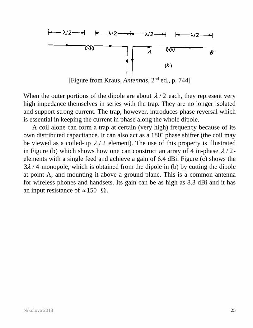
[Figure from Kraus, Antennas, 2nd ed., p. 744]

When the outer portions of the dipole are about / 2λ each, they represent very high impedance themselves in series with the trap. They are no longer isolated and support strong current. The trap, however, introduces phase reversal which is essential in keeping the current in phase along the whole dipole.

A coil alone can form a trap at certain (very high) frequency because of its own distributed capacitance. It can also act as a 180 phase shifter (the coil may be viewed as a coiled-up / 2λ element). The use of this property is illustrated in Figure (b) which shows how one can construct an array of 4 in-phase / 2λ -elements with a single feed and achieve a gain of 6.4 dBi. Figure (c) shows the 3 / 4λ monopole, which is obtained from the dipole in (b) by cutting the dipole at point A, and mounting it above a ground plane. This is a common antenna for wireless phones and handsets. Its gain can be as high as 8.3 dBi and it has an input resistance of 150≈ Ω .