Monitoring Traffic and Emissions by Floating Car Data

INSTITUTE OF TRANSPORT STUDIES The Australian Key Centre in Transport Management

The University of Sydney and Monash University Established under the Australian Research Council’s Key Centre Program.

WORKING PAPER ITS-WP-04-07

Monitoring Traffic and Emissions by Floating Car Data By

Astrid Gühnemann* ([email protected])

Ralf-Peter Schäfer ([email protected])

Kai-Uwe Thiessenhusen ([email protected])

Peter Wagner ([email protected]) March 2004 DLR - German Aerospace Centre Institute of Transport Research Rutherfordstr. 2 D - 12489 Berlin

*Visiting Scientist at ITS Sydney Sept. – Dec. 2003

NUMBER: Working Paper ITS-WP-04-07 TITLE: Monitoring Traffic and Emissions by Floating Car Data

ABSTRACT: Intelligent traffic management is widely acknowledged as a

means to optimise the utilisation of existing infrastructure capacities. A major requirement for intelligent traffic management is the collection of high quality data on traffic conditions in order to generate accurate real-time traffic information. The approach to be described here generates this information by a fleet of taxis equipped with GPS which act as Floating-Car-Data (FCD) provider for a number of metropolitan areas. The first part of this paper describes the methodology of setting up this data base. The information collected enables various applications such as real-time traffic monitoring, time-dynamic routing and fleet management. The second part of the paper proposes a framework for using these data additionally to include environmental effects into intelligent traffic management systems. To this end, a mapping between travel times and traffic flows is proposed. Some challenges related to the computation of emissions from velocity profiles are discussed. Equipped with these ingredients, an environmentally friendly intelligent traffic management might be in reach.

KEYWORDS: Floating-Car-Data, Traffic Monitoring, Traffic Management, Emission Modelling

AUTHORS: Astrid Gühnemann,* Ralf-Peter Schäfer, Kai-Uwe

Thiessenhusen and Peter Wagner. CONTACT: Institute of Transport Studies (Sydney & Monash) The Australian Key Centre in Transport Management, C37

The University of Sydney NSW 2006, Australia

Telephone: +61 9351 0071 Facsimile: +61 9351 0088 E-mail: [email protected] Internet: http://www.its.usyd.edu.au DATE: March 2004 *The research for this paper was done Dr Astrid Gühnemann was a Visiting Scientist at ITS, Sydney during September – December 2003.

Monitoring Traffic and Emissions by Floating Car Data Gühnemann, Schäfer, Thiessenhusen & Wagner

1

1. Introduction Conventional traffic monitoring systems that use stationary detectors such as counting loops do not produce reliable information about travel times within the network. The reason for this is that especially in urban areas their density is usually fairly low (the city of Berlin has about 200 of such devices), and the disturbances in urban areas is very high, so they cannot produce velocity profiles needed to compute travel times. Therefore, different techniques have been developed to measure travel times directly. Apart from simulation approaches that try to reconstruct the missing information from scarce data, other techniques such as license plate recognition, video imaging, or airborne traffic measurement are under development or even functional. However, in order to cover the traffic of metropolitan areas completely in time and space, these technologies are yet too costly. Therefore, the floating car data (FCD) technique has moved into the focus of current research, and first commercial applications have been developed. In the FCD-approach travel times and routes are determined directly from monitoring vehicles which ‘float’ with the traffic and whose position is determined by means of navigation technologies such as GPS (Global Positioning System). The pilot operation of commercial FCD based traffic information systems has shown that a sufficiently large number of vehicles have to be observed in order to derive reliable information. BURR, SIMMONS (2002) e.g. estimate these to about 1% of the total fleet. Another obstacle to providing successful commercial services based on FCD are the high communication costs which occur at today’s price levels for mobile communication when repeatedly transmitting vehicle positions and speed to a central server. Not least, generally a wider dissemination of intelligent traffic information services might have been hindered due to missing consumer’s acceptance, which had not been regarded sufficiently and therefore led to inadequate business models. In order to overcome some of these problems, an alternative FCD technique is described in this paper which presents a solution to the critical mass problem of probe vehicles by using data from taxis. This approach allows for a real-time, high-quality and low cost solution to traffic monitoring especially in urban areas. Furthermore, these data are an excellent basis for data mining analysing the daily variation of travel time on urban roads. Based on this information, applications have been developed such as real-time traffic jam detection and dynamic routing and navigation tools. Under the notion of establishing intelligent traffic management for environmentally sustainable transport solutions, these data are then applied for the development of dynamic emission models as a basis for an environmental monitoring and management of road traffic.

2. Establishing the Taxi-FCD Data Base 2.1 System Architecture The FCD data base in this project is fuelled by data from car fleets where the cars are equipped which GPS (Global Positioning System). The GPS-receiver in the car determines the position, with an error of 10 to 20 m, which is then transmitted to a


2

central server via a special operator’s broadcast system or via mobile communication such as GSM. Nowadays an increasing number of commercial vehicles are equipped with such GPS devices. The approach described here utilises data from the fleet management systems of taxi companies. The big advantage of this system is that no additional expenses for on-board equipment of vehicles or for software at the server site of the taxi headquarters are needed. Furthermore, the transfer of data happens by piggybacking them on the communication system needed by the taxi company anyway. Figure 1 shows the general architecture of the system. Thus, the taxis can easily be used as cheap probe vehicles for an extensive floating car data base. Using those commercial vehicles has a further advantage, which is their much higher utilization than private vehicles. In a most recent survey for Germany by IVS ET AL. (2003) the data show that vehicles which are used for commercial purposes travel about twice the distance of privately owned vehicles. A special advantage of using Taxis is their coverage of cities. In order to prove this concept a pilot system –running in different German and European cities– has been established. Since April 2001, more than 30 million GPS data have been recorded for Berlin already, other applications of this system are running in Vienna, Munich, Nuremberg, Stuttgart and Regensburg. This data provides the basis for further exploitation of traffic information in a high coverage and resolution of time and space as well as for the further development of service applications.

Control RoomDispatch

Management

TrunkedRadio Channel,

approx. 1-4 pos./ min

FCD Data BaseData Processing

Service ProviderData Utilization

GPRS, SMS,RDS-TMC, HTTP

...

Figure 1: System Architecture of the Taxi-FCD-System


3

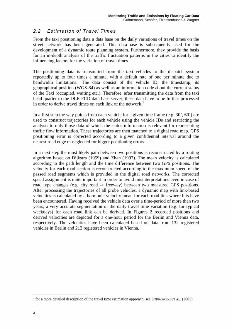
2.2 Estimation of Travel Times From the taxi positioning data a data base on the daily variations of travel times on the street network has been generated. This data-base is subsequently used for the development of a dynamic route planning system. Furthermore, they provide the basis for an in-depth analysis of the traffic fluctuation patterns in the cities to identify the influencing factors for the variation of travel times. The positioning data is transmitted from the taxi vehicles to the dispatch system repeatedly up to four times a minute, with a default rate of one per minute due to bandwidth limitations.. The data consist of the vehicle ID, the timestamp, its geographical position (WGS-84) as well as an information code about the current status of the Taxi (occupied, waiting etc.). Therefore, after transmitting the data from the taxi head quarter to the DLR FCD data base server, these data have to be further processed in order to derive travel times on each link of the network.1 In a first step the way points from each vehicle for a given time frame (e.g. 30’, 60’) are used to construct trajectories for each vehicle using the vehicle IDs and restricting the analysis to only those data of which the status information is relevant for representing traffic flow information. These trajectories are then matched to a digital road map. GPS positioning error is corrected according to a given confidential interval around the nearest road edge or neglected for bigger positioning errors. In a next step the most likely path between two positions is reconstructed by a routing algorithm based on Dijkstra (1959) and Zhan (1997). The mean velocity is calculated according to the path length and the time difference between two GPS positions. The velocity for each road section is reconstructed according to the maximum speed of the passed road segments which is provided in the digital road networks. The corrected speed assignment is quite important in order to avoid misinterpretations even in case of road type changes (e.g. city road -> freeway) between two measured GPS positions. After processing the trajectories of all probe vehicles, a dynamic map with link-based velocities is calculated by a harmonic velocity mean for each road link where hits have been encountered. Having received the vehicle data over a time-period of more than two years, a very accurate segmentation of the daily travel time variation (e.g. for typical weekdays) for each road link can be derived. In Figures 2 recorded positions and derived velocities are depicted for a one-hour period for the Berlin and Vienna data, respectively. The velocities have been calculated based on data from 132 registered vehicles in Berlin and 212 registered vehicles in Vienna.

1 for a more detailed description of the travel time estimation approach, see LORKOWSKI ET AL. (2003)


4

Figure 2: Positions (left) and derived velocities (right) from FCD in Berlin (top) and Vienna (bottom). Data are sampled over one hour. (SCHÄFER ET AL. (2003))

Following this procedure, a time-dynamic road map of historic and real-time link-based velocities becomes available, which is the input for several service applications as well as traffic monitoring purposes.

3. Applications for Individual Travel Services and Traffic Monitoring

Traffic congestion is perceived as a major problem in urban areas today. Clearly, only moderate extensions of the transport infrastructure are possible. Therefore, ITS (Intelligent Transport Systems) are regarded a potential alternative means for traffic management for decreasing congestion. Depending on the intensity with which measures can be implemented (e.g. share of vehicles equipped with dynamic routing systems or the utilization of adaptive traffic signal control systems) and the specific situation, PROGNOS AND KELLER (2001) estimate an increase in network capacities by 3% to 10% for Germany. In this view, several metropolitan areas and cities have set up traffic management centres with the aim to provide central access to improved traffic information for users (e.g. in Berlin) or even carrying out adaptive traffic control measures actively (e.g. in Sydney or Tokyo).


5

In order to design appropriate traffic management strategies, monitoring the performance of the transport network as a whole is necessary. This requires comprehensive data on the traffic states of the networks. Presently, the transport management centres rely on data that is collected from specific known hot spots by stationary measures, camera surveillance, as well as police observations and recordings. FCD technology provides an additional data base for monitoring the complete network. Furthermore, it is important to develop performance indicators that quantify congestion and are easy to understand. From the user’s perspective the main impact of congestion is the loss of travel time. Therefore, as e.g. QUIROGA (2000, p. 290) points out, travel-time based measures are advantageous compared to capacity or queuing-related measures because they are easily understood by user’s as well as traffic managers. Given sufficient data, they can be applied for specific locations as well as whole networks, allow for inter-temporal comparisons and can be easily translated into evaluation measures such as user costs. The travel-time based traffic maps that has been developed in this project are up to this task. These maps can then be applied for traffic monitoring purposes as well as individual travel services such as dynamic routing and navigation. In contrast to conventional router systems where static travel times are used, the routing service based on FCD use real-time information and –if these are not available– the "experiences" of the associated taxi fleets to provide users with high-quality routing information.

Figure 3: Traffic state in Vienna at 3.6.03, early in the morning (7:29) and three hours later (10:29).

At this day, the employees of the public transport went on strike.

3.1 Dynamic Routing and Navigation

In order to calculate the fastest route for a given journey, conventional routing and navigation systems usually apply average velocities which are derived from default and static link-based speed values. For the Navtech® digital network of Berlin, on the average these values show a good representation of the average daily values which have observed using the Taxi FCD. A more detailed analysis shows, however, that for urban freeways, arterial and major routes, FCD velocities were 6.3 km/h lower than the speeds provided by the Navtech® data-base. This is less than the 10-20 km/h speed category


6

band width that Navtech® applies. However, on smaller urban roads the difference reaches more than 20 km/h. Furthermore, the average velocities calculated from the FCD data vary considerably during the hours of the day and between links. In consequence, there is a high probability that the average speed values differ considerably from the real values for specific links and during the day and hence, the proposed route and travel time estimation deliver an unrealistic advice. Of course, this difficulty could be overcome if the digital road map attributes are changed from static velocity parameter to real-time measurement from the probe vehicles or at least to historic measurements from a similar period of the past. For demonstration of the differences between the static link-velocity estimations and the link velocities derived from FCD a plot of the Berlin city centre is visualised.

Figure 4: Berlin, historical measurements by Taxi-FCD for the afternoon rush-hour (left), Navtech® Speed types (right)

In order to demonstrate the described benefits of a dynamic routing and navigation system a web-based portal has been developed. The routing server, using a Dijkstra optimisation algorithm, can be operated in different modes, one for real-time optimisation and the other mode for pre-trip planning of a certain journey. In the real-time mode each link of the digital road network is loaded by an average travel time of Taxi floating car data measurements on this road link during the last 30 minutes, by default. In case that no Taxi passed this road link, historical travel time measurements related to the current weekday and time of the day are used. The route optimisation can be chosen by various criteria, calculating the shortest, fastest or cost-efficient path. The routing server can be accessed by various interfaces and devices like a Web Browser, mobile phone or personal digital assistants (PDA). In order to use the routing service on-board the car, a PDA-based off-board navigation system was implemented. This solution has several advantages. The real-time use allows an on-trip optimisation during a journey. Due to the dynamic route optimisation outside the vehicle, real-time traffic data can be considered allowing to bypass a congested region of the city. Furthermore, the digital road map has only to be updated on the server site. Due to the fact that the route is calculated on the server site for each optimisation a certain amount of data have to be transferred between the server and the vehicle. For the data transfer a package-oriented wireless communication service (GPRS) is used which guarantees low expenses for the data transfer.


7

The FCD basis and the route planning system described above are accessible at http://www.cityrouter.net.org. On the one hand, future commercial services such as fleet management systems could also profit from this data base, on the other hand, this data can be applied to develop improved methodologies for measuring the transport networks’ performance in urban areas, in particular with respect to congestion and environmental impacts.

4. Application for Emission Monitoring

From the public perspective, a further requirement for the development of traffic management strategies is information on environmental and other adverse effects, e.g. to prevent routing through sensitive areas. This requires additional information that has to be generated for the total quantities of traffic on the network segments and for the corresponding environmental impacts. In the following, an approach is presented for computing the emissions of traffic which takes advantage of the temporal and spatial resolution of the Taxi floating car data base. There are three building blocks to this approach: in a first step, the dependence between traffic flow and travel times has to be analyzed. This will lead to a rule-set for deriving flows from travel times. This is necessary, since the FCD provide travel times, but no traffic volumes. Second, the travel times need to be broken down into speed profiles, which of course is very difficult if the distance between subsequent positions becomes too big. Third, the emissions have to be computed from these profiles. This is made more complicated by the fact that usually emission factors are meant as kind of averages, but here truly time- and load-dependent emissions are needed.

4.1 Data Analysis of GPS Taxi-FCD As discussed, to compute emissions first of all the corresponding flows are needed. The floating car data contain just the travel times and velocities that have been observed in the network, but flows are not directly measured. The relation between these quantities is in principle provided by the fundamental diagram, which comes in many flavours for different types of road, speed limits, signalized and un-signalized arterials to name but a few as e.g. applied in the US Highway Capacity Manual. Fundamental diagrams for these conditions show that in a broad range of fairly free traffic flow, speed is nearly constant and independent of traffic density. With the increase of traffic density disturbances between vehicles grow and the speed decreases down to traffic jams and total traffic breakdown at a maximum density (and zero flows). This corresponds with the well-known basic principles of traffic flow theory (e.g. published in LEUTZBACH, 1972). There are two caveats, though. Firstly, fundamental diagrams usually apply to spot measurements, so within the context to be derived here, a kind of fundamental diagram between flow and space mean speed (proportional to inverse travel time) has to be derived. Secondly, inverting the function (usually speed depends on density) in order to estimate traffic densities or flows from observed velocities is difficult. Especially in the


8

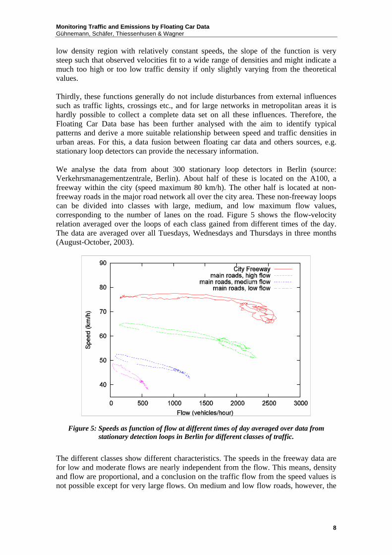
low density region with relatively constant speeds, the slope of the function is very steep such that observed velocities fit to a wide range of densities and might indicate a much too high or too low traffic density if only slightly varying from the theoretical values. Thirdly, these functions generally do not include disturbances from external influences such as traffic lights, crossings etc., and for large networks in metropolitan areas it is hardly possible to collect a complete data set on all these influences. Therefore, the Floating Car Data base has been further analysed with the aim to identify typical patterns and derive a more suitable relationship between speed and traffic densities in urban areas. For this, a data fusion between floating car data and others sources, e.g. stationary loop detectors can provide the necessary information. We analyse the data from about 300 stationary loop detectors in Berlin (source: Verkehrsmanagementzentrale, Berlin). About half of these is located on the A100, a freeway within the city (speed maximum 80 km/h). The other half is located at non-freeway roads in the major road network all over the city area. These non-freeway loops can be divided into classes with large, medium, and low maximum flow values, corresponding to the number of lanes on the road. Figure 5 shows the flow-velocity relation averaged over the loops of each class gained from different times of the day. The data are averaged over all Tuesdays, Wednesdays and Thursdays in three months (August-October, 2003).

Figure 5: Speeds as function of flow at different times of day averaged over data from stationary detection loops in Berlin for different classes of traffic.

The different classes show different characteristics. The speeds in the freeway data are for low and moderate flows are nearly independent from the flow. This means, density and flow are proportional, and a conclusion on the traffic flow from the speed values is not possible except for very large flows. On medium and low flow roads, however, the


9

speed is reduced with growing flow even for low flows. Here it is possible to conclude from the speed on the flow.

Figure 6: Daily speed profiles from stationary detection loops (upper curve) and from FCD (middle curve) averaged over Tuesdays-Thursdays at the inner part of Berlin. Lower curve:

corresponding daily flow profile from stationary detection loops averaged over the same time period and region.

In Figure 6, the daily speed profiles from FCD and stationary data are compared. The data are averaged over the same period as in Fig. 4 and over a 6 km x 10 km area in the inner part of Berlin. Freeway data are not taken into account. FCD as well as loop detector speed profiles follow similar characteristics. The speed is lowest in the morning and – especially – the afternoon rush hour where the average citywide flow has its maximum. Obviously, there is a large difference in the absolute values of speed between these two approaches. The loop detectors speeds are about 50% larger than the FCD speeds. The reason is simple: nearly all of the detectors are located at road sections away from major intersections. Therefore, the measured speeds to not contain loss times during stops at intersections caused, e.g., by traffic signals or merging traffic. In contrast, the FCD speeds are a measure for the real trip speed including such stops. A comparison of these two speed values leads to an estimated value for the fraction of stop time at the total trip time of about 0.3, which is in good accordance with previous measurements, see e.g. HERMAN, ARDEKANI (1984). Figure 7 shows as an example the situation along an arterial road section in Berlin (Beusselstr., direction to the South). The FCD speed is averaged as function of position on the road section.


10

Figure 7: Local speed profile (day average) reconstructed on an arterial road “section Beusselstraße” (1.2 km) from FCD. There is a signalized intersections at x=0.38, 0.47km,

and 0.94 km. The speed profile exhibits a number of speed drops. The main drops are at the positions of intersections controlled by traffic signals. Note that the sample rate of 30s of the FCD analysed here leads to a slight smoothing of the speed profile. By integration of the speed along the way, the travel times can be calculated. Detection loops are located away from the intersections. At their locations the speed is typically above average. (E.g, in this plot there are loop detectors at x=0.06 and x=0.81. Their data have been taken into account in the plots in Fig. 4 and 5.). Therefore, a way to obtain a reasonable flow-speed relation can be to consider speed values from FCD and flows from the stationary loop detectors. Unlike the speed, the flow has no short-scaled local variations. So flows measured with stationary detectors are valid at least for the whole road section. If the distribution of loop detectors is representative enough, such analysis can be performed either for typical roads of a specific class as well as for selected regions of a city. 4.1 Estimation of Traffic Flows The general aim is to calculate the total emissions that are produced on the Berlin networks within an observed time period. Therefore, traffic flows have been derived from the FCD base using the calculated velocities and the information on speed profiles and speed-flow relationships from the previous section considering all the uncertainties that this estimation includes as described earlier in this paper. The basis for this calculation and the following development of the dynamic emission model are taxi FCD that have been collected over a one year period (June 2002 to May


11

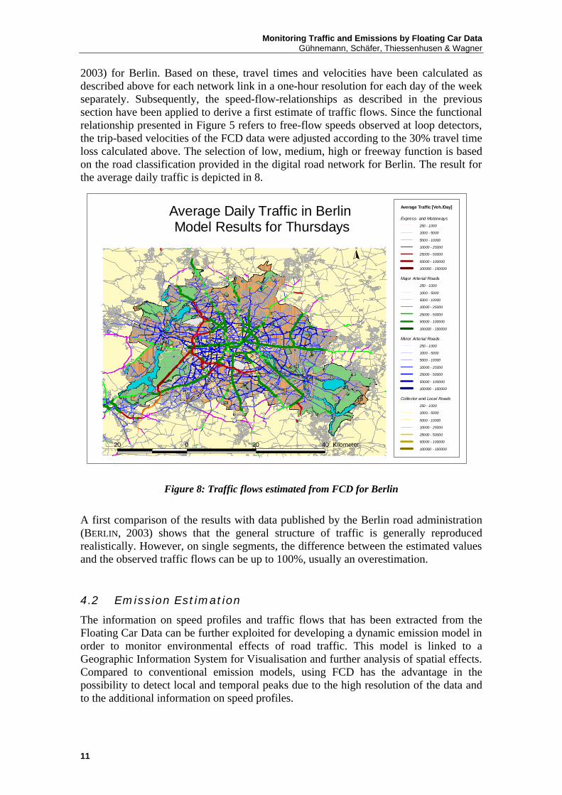
2003) for Berlin. Based on these, travel times and velocities have been calculated as described above for each network link in a one-hour resolution for each day of the week separately. Subsequently, the speed-flow-relationships as described in the previous section have been applied to derive a first estimate of traffic flows. Since the functional relationship presented in Figure 5 refers to free-flow speeds observed at loop detectors, the trip-based velocities of the FCD data were adjusted according to the 30% travel time loss calculated above. The selection of low, medium, high or freeway function is based on the road classification provided in the digital road network for Berlin. The result for the average daily traffic is depicted in 8.

N

Average Daily Traffic in Berlin Model Results for Thursdays

Express- and Motorways

250 - 1000

1000 - 5000

5000 - 10000

10000 - 25000

25000 - 50000

50000 - 100000

100000 - 150000

Major Arterial Roads

250 - 1000

1000 - 5000

5000 - 10000

10000 - 25000

25000 - 50000

50000 - 100000

100000 - 150000

Minor Arterial Roads

250 - 1000

1000 - 5000

5000 - 10000

10000 - 25000

25000 - 50000

50000 - 100000

100000 - 150000

Collector and Local Roads

250 - 1000

1000 - 5000

5000 - 10000

10000 - 25000

25000 - 50000

50000 - 100000

100000 - 150000

Average Traffic [Veh./Day]

20 0 20 40 Kilometer

Figure 8: Traffic flows estimated from FCD for Berlin

A first comparison of the results with data published by the Berlin road administration (BERLIN, 2003) shows that the general structure of traffic is generally reproduced realistically. However, on single segments, the difference between the estimated values and the observed traffic flows can be up to 100%, usually an overestimation. 4.2 Emission Estimation The information on speed profiles and traffic flows that has been extracted from the Floating Car Data can be further exploited for developing a dynamic emission model in order to monitor environmental effects of road traffic. This model is linked to a Geographic Information System for Visualisation and further analysis of spatial effects. Compared to conventional emission models, using FCD has the advantage in the possibility to detect local and temporal peaks due to the high resolution of the data and to the additional information on speed profiles.


12

For the calculation of emissions, different approaches are available which can be adapted for our purposes. Generally, road traffic emissions consist of three major parts: Cold start emissions, hot emissions and evaporative emissions (see e.g. HICKMAN ET AL. (1999)). Due to lack of data, cold start emissions are most often calculated as a constant per trip. From the FCD data, trip data for all vehicles cannot be extracted. Therefore, cold start emissions can only be assigned to the network links randomly or equally distributed, or as a probability function of trip origins. A similar procedure would have to be applied for evaporative emissions, which occur during refuelling or time dependently due to temperature increases. Another level of uncertainty comes from the lack of data on the fleet composition on a specific link at a specific time. Especially so-called “gross” or “super emitters”, i.e. uncontrolled, badly maintained or malfunctioning vehicles, as well as emissions from cars operating on high engine load on freeways are considered to be a source for a substantial proportion of overall emissions, e.g. in GOMES (2001) or JOURMARD ET AL. (1999). Therefore, in order to identify the areas which are most affected by road traffic emissions, we restrict our calculations to hot emissions of an average fleet. However, it must be kept in mind that the total level of emissions calculated per link is probably an underestimation due to the omissions mentioned above. In some approaches, e.g. the Handbook of Emission Factors by INFRAS (1999), average emission rates are provided for defined traffic states (e.g. congested in urban areas, free flow < 100 km/h on freeways etc.), others such as HICKMAN ET AL. (1999) provide speed dependent factors. For our project, a velocity dependent approach is more appropriate because it can take advantage of the high resolution of our data. For lack of data on the car fleet in Berlin, average German values are applied which are provided in CERWENKA ET AL. (2002). Additionally, the German average share of diesel vehicles of 18.3% is applied for all road segments, shares of heavy vehicles are kept constant differentiated by road types. By applying the speed profiles from the analysis of the FCD it is further possible to include the influences of variations is speeds. This has been made exemplary for the speed profile depicted in Figure 7. In a first approach, emissions due to acceleration processes have been neglected due to lack of data. Figure 9 shows the difference in results of the emission calculation for a single car using the velocity values of the speed profiles or the speed average over the whole road section. For NOx emissions of petrol cars, the difference adds up to about 20%, for diesel vehicles to 30%.


13

NOx Emission Profile Diesel Cars

0.4

0.5

0.6

0.7

0.8

0.9

1

0 0.1 0.2 0.3 0.4 0.5 0.6 0.7 0.8 0.9 1 1.1

Distance (km)

Em

issi

on

s (g

)

Speed Profile Speed Average

NOx Emission Profile Petrol Cars

1

1.1

1.2

1.3

1.4

1.5

1.6

0 0.1 0.2 0.3 0.4 0.5 0.6 0.7 0.8 0.9 1 1.1

Distance (km)

Em

issi

on

s (g

)

Speed Profile (Petrol) Speed Average

Figure 9: Difference between NOx-emissions calculated based on speed profiles or speed average

In order to depict the spatial distribution of emissions, the road link based values are assigned to a standardised emission cataster using an equal area size grid. For this purpose a grid which is applied for the European EMEP-Programme (Co-operative Programme for Monitoring and Evaluation of the Long-Range Transmission of Air Pollutants in Europe) has been used but scaled down to a resolution of 200m x 200m to account for the requirements of urban traffic management (see Figure 10). This achieves a full spatial coverage of the area of Berlin. Together with the temporal resolution of the FCD this allows for the identification of local hot spots.

NOx Emissions [kg]0 value0 - 250250 - 500500 - 10001000 - 20002000 - 5000

N

EW

S

NOx-EmissionsModel Results Thursdays (4 p.m - 5 p.m.)

10 0 10 20 Kilometer

Figure 10: Model results for the regional distribution of transport emissions in Berlin


14

4.4 Population Affected by Emissions To evaluate the impacts of traffic on environment and population, emission values are just a first indicator covering the pressures that are imposed. Further analysis is necessary to assess impacts on or changes in environmental or health state. As a first indicator of disturbances, the number of inhabitants that are exposed to the pressures (here emissions) can be calculated. The aim is to reduce the exposure of the population to below defined threshold values for as many inhabitants as possible. Figure 11 depicts the population density in Berlin, which shows a structure of multiple centres which group around the city centre that is characterised by historical, governmental, and business buildings as well as a large park (“Tiergarten”).

0 6 12 18 KilometerS

N

EW

Population Density in Berlin (Jan 2003)

Institute of Transport Research DLR 2003

Data Source:Statistisches Landesamt Berlin

Inhabitants per sqkm

0 - 750

750 - 2250

2250 - 3000

3000 - 4000

4000 - 5000

5000 - 6500

6500 - 10000

10000 - 16500

16500 - 24000

24000 - 35000

35000 - 110000

Other Areas

Railway Property

Green / Park

Water

Traffic Zones

Population Density

Figure 11: Population Density in Berlin (by block areas, ranges based on quantiles)

This ring structure can also be observed in the road and urban rail networks that connect these centres. Therefore, quite naturally high traffic and emission values most often occur just in the densely populated areas. By the application of Geographical Information System tools it is possible to overlay the estimated emission values with the population densities to further analyse the results with respect to potential effects on or risks for the Berlin population. Figure 12 shows the results for a sector around the Berlin city centre. Population densities are coloured red, emissions blue. This means, the darker purple an area is, the higher is the disturbance of population due to emissions measured by the indicator


15

inhabitants x emissions. Overall, according to these still preliminary results, 15 % of the inhabitants live in the most pressured areas (90% quantile of grid cell emission values). Using these tools for modelling and visualizing the pressures imposed on the population it is also possible to monitor the development over time using the taxi FCD that are collected continuously.

Figure 12: Population Affected by Transport Emissions in Berlin Centre (9-10 a.m, Thursdays). The darkest purple areas indicate the highest exposure measured by inhabitants

x emissions.

5 Conclusions and Further Research Activities In this paper we have demonstrated the potential of FCD to improve the measurement of travel times in metropolitan areas and to use these data for traffic management and emission monitoring purposes. Based on hundreds of probe vehicles it is now possible to measure traffic state variables in a high temporal and spatial resolution, with a high coverage of urban areas where the coverage by other sensors is low, and at low costs. The recorded GPS positioning data of the probe vehicles offer a range of possibilities for data analysis of traffic patterns in urban areas and as a basis for individual travel service applications as well as traffic monitoring and management. In order to show the advantages of the FCD approach several applications like dynamic routing and navigation, traffic monitoring, traffic jam detection as well as methods how to use spatial traffic information for a real-time monitoring environmental effects of traffic were discussed.

Population Density [Inh./sqkm]1 - 500500 - 10001000 - 25002500 - 50005000 - 75007500 - 1000010000 - 2500025000 - 5000050000 - 100000100000 - 250000No Data

Emissionen NOx [kg/a]00 - 250250 - 500500 - 10001000 - 20002000 - 5000

5 0 5 10 15 Kilometer

N

EW

S

Population Exposure to NOx-Emissions


16

However, there are still many research challenges in further exploiting the data base and its applications. Firstly, additional information can be gained by further data analysis and data mining techniques, for example, by using correlations between travel times on connecting roads. It will be necessary to evaluate the congestion warning, travel time calculations, route recommendations and traffic flow estimations with other data sets available or own measurements. A subsequent step will be to include short term forecasts which are developed either by data mining techniques or by means of micro-simulation models. For traffic management and monitoring purposes, it will be necessary to include other effects than emissions by taking indicators e.g. for accidents, noise or economic impacts into account. These have to be condensed to a limited set of core indicators in order to keep it manageable for decision makers. There is a large quantity on literature on environmental indicators and targets, some of which can easily applied for urban areas, e.g. noise exposure levels. However, for others such as CO2 emissions the transformation from global to urban level is much less obvious, and for many impacts a dose-response relationship is either very complex or unclear, especially for social impacts. The full strength of the FCD approach will be gained by the data fusion in progress with data from other sources such as stationary or remote sensing technologies.

References

Berlin (2003): Senatsverwaltung für Stadtentwicklung: mobil 2010 – Stadtentwicklungsplan Verkehr, Entwurf (downloadable from website: http://www.stadtentwicklung. berlin.de/planen/stadtentwicklungsplanung/de/verkehr/download.shtml)

Burr, J., Simmons, N.: Floating Vehicle Data – Number of Probes for Real Time Coverage, ITS World Congress, Chicago, 2002, http://194.203.66.39/its_assist/files/ITS_World_ Congress_Paper_Floating_Vehicle.pdf

Cerwenka, P., Dischinger, N., Klamer, M., Walther, C. (2002): Anwendungsorientierte Ermittlung von Kraftstoffverbrauch und Schadstoffemissionen des Kraftfahrzeugverkehrs in Deutschland für die Neufassung der RAS-W (EWS): In: FGSV: WirtschaftlichkeitsuntersuchungenWirtschaftlichkeitsuntersuchungen an Straßen – Stand und Weiterentwicklungen der EWS, Köln, pp.15-23

Dijkstra, E.W. (1959): A Note on two Problems in Connections with Graphs, Numerische Mathematik, 1:269-271.

Gomes, J.A.G (2001): Impacts of Road Traffic Emissions on the Ozone Formation in Germany. Dissertation. Bergische Universität-Gesamthochschule Wuppertal

Herman, R., Ardekani, S (1984), Characterizing Traffic Conditions in Urban Areas, Transportation Science, 18, 101-140

Lorkowski, S., Brockfeld, E., Mieth, P., Passfeld, B., Thiessenhusen, K.-U. Schäfer, R.-P. (2003): Erste Mobilitätsdienste auf Basis von Floating Car Data. In: Institut für Stadtbauwesen und Verkehr, RWTH Aachen [Hrsg.]: Tagungsband zum 4. Aachener


17

Kollouium Mobilität und Stadt, Band 75, Jahrgang 2003, Reihe Stadt Region Land, S. 93-100, 4. Aachener Kolloquium Mobilität und Stadt; AMUS, 31.7.-1.8.2003, Aachen.

Hickman, J. (editor), Hassel, D., Joumard, R., Samaras, Z., Sorenson, S. (1999) : Methodology for Calculating Transport Emissions and Energy Consumption. Deliverable 22 for the project MEET (Methodologies for estimating air pollutant emissions from transport). Project funded by the European Commission under the Transport RTD programme of the 4th Framework programme. Contract No. ST-96-SC.204. Co-sponsored by the Driver Information and Traffic Management Division of the Department of the Environment, Transport and the Regions. In conjunction with COST Action 319. Project Report SE/491/98, TRL Transport Research Laboratory, Crowthorne, UK

INFRAS (1999): Handbuch für Emissionsfaktoren HBEFA, Version 1.2, Bern

IVS (Institut für Verkehr und Stadtbauwesen, Technische Universität Braunschweig), IVT (Institut für angewandte Verkehrs- und Tourismusforschung), WVI (Prof. Dr. Wermuth Verkehrsforschung und Infrastrukturplanung), KBA (Kraftfahrt-Bundesamt), P.U.T.V (Projektforschung, Unternehmensberatung, Transport und Verkehr): Konti-nuierliche Befragung des Wirtschaftsverkehrs in unterschiedlichen Siedlungsräumen - Phase 2, Hauptstudie (Kraftfahrzeugverkehr in Deutschland - KiD 2002), Project No. 70.0682/2001 on behalf of the German Ministry of Transport and Regional Planning, Final Report, Braunschweig

Joumard, Robert ; Philippe, Franck ; Vidon, Robert (1999) : Reliability of the current models of instantaneous pollutant emissions. The Science of the Total Environment 235 1999 133]142

Leutzbach, W. (1972): Einführung in die Theorie des Verkehrsflusses. Springer Verlag Berlin – Heidelberg - New York

Prognos AG, Keller, H. (2001): Wirkungspotentiale der Verkehrstelematik zur Verbesserung der Verkehrsinfrastruktur und Verkehrsmittelnutzung. Im Auftrag des Bundesministeriums für Verkehr, Bau- und Wohnungswesen, Berlin (FE-Nr. 96.584/1999), Prognos Berichte 581-5466, Basel

Quiroga, Cesar A. (2000): Performance measures and data requirements for congestion management systems. In: Transportation Research Part C 8 (2000) pp. 287 – 306

Schäfer, R.-P., Thiessenhusen, K.-U., Brockfeld, E. and Wagner, P. (2002): Analysis of Travel Times and Routes on Urban Roads by Means of Floating-car Data, Proceedings of the ITS World Congress 2002, Chicago, USA.

Schäfer, Ralf-Peter, Gühnemann, Astrid, Thiessenhusen, Kai-Uwe: Neue Ansätze im Verkehrsmonitoring durch Floating Car Daten. 19. Verkehrswissenschaftliche Tage "Mobilität und Verkehrsmanagement in einer vernetzten Welt", 22. bis 23. September 2003, Technische Universität Dresden

Zhan, F.B. (1997): Three Fastest Shortest Path Algorithms on Real Road Networks: Data Structures and Procedures, Journal of Geographic Information and Decision Analysis, vol. 1, no.1, pp. 69 – 82.

Monitoring Traffic and Emissions by Floating Car Data

Documents

Transcript of Monitoring Traffic and Emissions by Floating Car Data