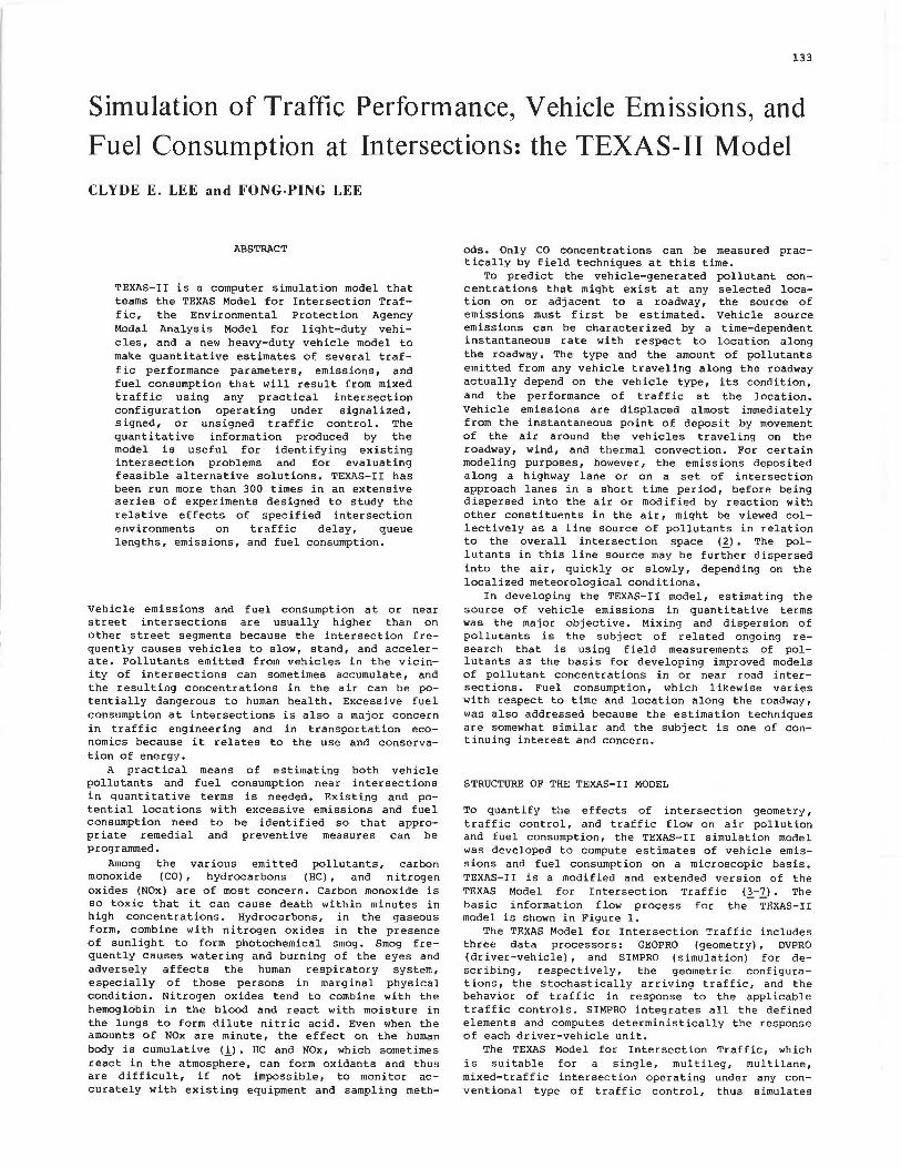
133

Simulation of Traffic Performance, Vehicle Emissions, and

Fuel Consumption at Intersections: the TEXAS-II Model

CLYDE E. LEE and FONG-PING LEE

ABSTRACT

TEXAS-II is a computer simulation model that teams the TEXAS Model for Intersection Traf­fic, the Environmental Protection Agency Modal Analysis Model for light-duty vehi­cles, and a new heavy-duty vehicle model to make quantitative estimates of several traf­fic performance parameters, emissions, and fuel consumption that will result from mixed traffic using any practical intersection configuration operating under signalized, signed, or unsigned traffic control. The quantitative information produced by the model is useful for identifying existing intersection problems and for evaluating feasible alternative solutions. TEXAS-II has been run more than 300 times in an extensive series of experiments designed to study the relative effects of specified intersection environments on traffic delay, queue lengths, emissions, and fuel consumption.

Vehicle emissions and fuel consumption at or near street intersections are usually higher than on other street segments because the intersection f re­quently causes vehicles to slow, stand, and acceler­ate. Pollutants emitted from vehicles in the vicin­ity of intersections can sometimes accumulate, and the resulting concentrations in the air can be po­tentially dangerous to human health. Excessive fuel consumption at intersections is also a major concern in traffic engineering and in transportation eco­nomics because it relates to the use and conserva­tion of energy.

A practical means of estimating both vehicle pollutants and fuel consumption near intersections in quantitative terms is needed. Existing and po­tential locations with excessive emissions and fuel consumption need to be identified so that appro­priate remedial and preventive measures can be programmed.

Among the various emitted pollutants, carbon monoxide (CO), hydrocarbons (HC), and nitrogen oxides (NOx) are of most concern. Carbon monoxide is so toxic that it can cause death within minutes in high concentrations. Hydrocarbons, in the gaseous form, combine with nitrogen oxides in the presence of sunlight to form photochemical smog. Smog fre­quently causes watering and burning of the eyes and adversely affects the human respiratory system, especially of those persons in marginal physical condition. Nitrogen oxides tend to combine with the hemoglobin in the blood and react with moisture in the lungs to form dilute nitric acid. Even when the amounts of NOx are minute, the effect on the human body is cumulative < .. !J. HC and NOx, which sometimes react in the atmosphere, can form oxidants and thus are difficult, if not impossible, to monitor ac­curately with existing equipment and sampling meth-

ods. Only CO concentrations can be measured prac­tically by field techniques at this time.

To predict the vehicle-generated pollutant con­centrations that might exist at any selected loca­tion on or adjacent to a roadway, the source of emissions must first be estimated. Vehicle source emissions can be characterized by a time-dependent instantaneous rate with respect to location along the roadway. The type and the amount of pollutants emitted from any vehicle traveling along the roadway actually depend on the vehicle type, its condition, and the performance of traffic at the location. Vehicle emissions are displaced almost immediately from the instantaneous point of deposit by movement of the air around the vehicles traveling on the roadway, wind, and thermal convection. For certain modeling purposes, however, the emissions deposited along a highway lane or on a set of intersection approach lanes in a short time period, before being dispersed into the air or modified by reaction with other constituents in the air, might be viewed col­lectively as a line source of pollutants in relation to the overall intersection space (~) • The pol-1 utants in this line source may be further dispersed into the air, quickly or slowly, depending on the localized meteorological conditions.

In developing the TEXAS-II model, estimating the source of vehicle emissions in quantitative terms was the major objective. Mixing and dispersion of pollutants is the subject of related ongoing re­search that is using field measurements of pol­lutants as the basis for developing improved models of pollutant concentrations in or near road inter­sections. Fuel consumption, which likewise varies with respect to time and location along the roadway, was also addressed because the estimation techniques are somewhat similar and the subject is one of con­tinuing interest and concern.

STRUCTURE OF THE TEXAS-II MODEL

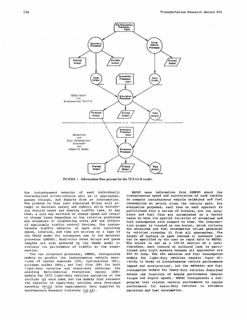
To quantify the effects of intersection geometry, traffic control, and traffic flow on air pollution and fuel consumption, the TEXAS-II simulation model was developed to compute estimates of vehicle emis­sions and fuel consumption on a microscopic basis. TEXAS-II is a modified and extended version of the TEXAS Model for Intersection Traffic (~-l>· The basic information flow process for the TEXAS-II model is shown in Figure 1.

The TEXAS Model for Intersection Traffic includes three data processors: GEOPRO (geometry), DVPRO (driver-vehicle), and SIMPRO (simulation) for de­scribing, respectively, the geometric configura­tions, the stochastically arriving traffic, and the behavior of traffic in response to the applicable traffic controls. SIMPRO integrates all the defined elements and computes deterministically the response of each driver-vehicle unit.

The TEXAS Model for Intersection Traffic, which is suitable for a single, multileg, multilane, mixed-traffic intersection operating under any con­ventional type of traffic control, thus simulates

134 Transportation Research Record 971

p,..Slmglolion ,roe111ot

Input

TEXAS Model for

Intersection Traffic

Emissions and

Fuel Consumption Processor

for TEXAS-II Model

Pvnchtd Ovlpvl

\

\ \

\ \ \

\ \

FIGURE 1 Information flow process for the TEXAS-II model.

the instantaneous behavior of each individually characterized driver-vehicle unit as it approaches, passes through, and departs from an intersection. The premise is that each simulated driver will at­tempt to maintain safety and comfort while sustain­ing desired speed and obeying traffic laws. At any time, a unit may maintain or change speed and retain or change lanes depending on the relative positions and movements of neighboring units and the effects of applicable traffic control devices. The instan­taneous traffic behavior of each unit including speed, location, and time are 'written on a tape by the TEXAS model for subsequent use in the emission processor (EMPRO) • Statistics about delays and queue lengths are also gathered by the TEXAS model to evaluate the performance of traffic at the inter­section.

The new emissions processor, EMPRO, incorporates models to predict the instantaneous vehicle emis­sions of carbon monoxide (CO) , hydrocarbons (HC) , nitrogen oxides (NOx), and fuel flow (FF) for both light-duty vehicles and heavy-duty vehicles. The existing Environmental Protection Agency (EPA) models for 1975 light-duty vehicles operating at low altitude (8) were used, but the models that estimate the behaviOr of heavy-duty vehicles were developed recently (2_-11) with experimental data supplied by Southwestern Research Institute (~-~) •

EMPRO uses information from SIMPRO about the instantaneous speed and acceleration of each vehicle to compute instantaneous vehicle emissions and fuel consumption at points along the vehicle path. For evaluation purposes, each lane on each approach is partitioned into a series of buckets, and the emis­sions and fuel flow are accumulated on a bucket basis to show the spatial variation of emissions and fuel consumption with respect to time. The intersec­tion proper is treated as one bucket, which collects the emissions and fuel consumption values generated by vehicles crossing it from all approaches. The length of buckets on each inbound or outbound lane can be specified by the user as input data to EMPRO. The bucket is set as a 100-ft section of a lane 1

therefore, each inbound or outbound lane is parti­tioned into eight buckets because all approaches are 800 ft long. The EPA emission and fuel consumption models for light-duty vehicles require input di­rectly in terms of instantaneous vehicle performance (speed and acceleration), but the emission and fuel consumption models for heavy-duty vehicles described herein use functions of engine performance (engine torque and engine speed). EMPRO incorporates a sub­program that relates vehicle performance to engine performance for heavy-duty vehicles to estimate

emissions and fuel consumption.

Lee and LeP.

Emissions and Fuel Consumption Models for Ligh t-Duty Vehic les

The emission models for co, HC, NOx and co2 devel­oped by EPA for light-duty vehicles and referred to as the Modal Analysis Model (_!!.), are presented in quadratic form of speeds for a steady state of vehi­cle motion, and in quadratic form of speeds and accelerations for transient states. The fuel con­sumption model is expressed as a linear function of the amounts of HC, co, and COz emitted. The emis­sion models are formulated as follows:

Steady state

where

L =instantaneous emission rate (grams/second), V speed (mph) , and s coefficients (given in Table 1).

Transient state

L(V, A) =B 1 + B2 V + B3A + B4 AV + B5 V2

+B6A2 +B7V2A+BaA2V+B9A2 V2

where

A • acceleration or deceleration (mph/second) and B • coefficients (given in Table 1).

In the Modal Analysis Model, vehicles are classified in 18 groups by model year from 1957 to 1975 and by low or high operating altitude. The 1975 low-alti­tude group, which provides the most current informa­tion that is generally available and matches the terrain situations of many American cities, was selected for use in the TEXAS-II model. The models

135

and coefficients for estimating the emissions of CO, HC, NOx, and co2 for the 1975 low-altitude group of automobiles are given in Table 1. These coeffi­cients can be modified by the user if necessary. An evaluation of the models indicates that in steady­state driving the emissions of CO and HC decrease with speed while the emissions of NOx and co2 increase with speed. The fuel consumption rate in s teady-state driving stays almost constant for speeds up to 10 mph and then increases with speed. In transient-state driving, acceleration increases emissions and fuel consumption. The effect of ac­celeration is higher when speed is higher. Use of the coefficients for the 1975 low-altitude group of vehicles can produce negative values of emissions and fuel flow. In the TEXAS-II model, all such negat i ve values are automatically set to zero.

Emissions a nd Fuel Consump tion Models for Heavy - Duty Vehicle s

A series of models (see Table 2) for estimating instantaneous values of emissions and fuel consump­tion for heavy-duty vehicles powered by gasoline or diesel engines was developed for incorporation into the data postprocessor called EMPRO in the TEXAS-II model. This development involved combining rational approximations of vehicle dimensions and operating characteristics with empirical data on engine per­formance to produce the models.

Experiments conducted at southwest Research In­stitute (12-19) indicated that emission rates from heavy-duty vehicles are functions of speed, acceler­ation, engine make, type of pollution control de­vices, maintenance condition, and engine operating temperature. These experiments involved testing a representative sample of heavy-duty vehicles (HOVs) and measuring the produced emissions for comparison with proposed regulatory standards. A 13-mode steady-state test schedule was used for diesel en-

TABLE 1 Instantaneous Emission and Fuel Consumption Models for Passenger Cars (8 )

INSTANTANEOUS EMISSION MODELS

Steady State Hodel : L(V) = 2 s1 + s2

v + s3

v

L - Instantaneous Emissions Rate {gram/second)

v . Speed (mph)

Transient State Model: L{V,A) - 2 2 2 2 2 2 Bl + B2V + B

3A + B

4 VA + B5V + B

6A + B

7V A+ B

8VA + B

9V A

A . Acceleration or Deceleration {H/H2)

COEFFICIENTS FOR EHI SS ION MODELS

State co HC NO c o 2 x

Sl l.16557780E - 01 5. 38159910E - 03 1. 46B95690E + 00 2.65079990E - 03 Ste~dy S2 -4. 62989880E - 03 -l.45500000E - 04 7. 066901BOE - 03 -3.53701l020E - 04

S3 6. 98999940E - 05 1. 999999BOE - 06 1. 61370010E - 03 2. 34 00004 0E - 05

Bl 2 .15785210E - 01 8.06840140E - 03 2. 28404900E + 00 l. 08160000E - 02 B2 -1. 257779BOE - 02 -4.00200020E - 04 -2. 62799000E - 02 -1. 22500000E - 03 B3 5.14772980E - 02 9. 00400100E - 04 6.55900840E - 02 -7. 354 OOOlOE - 04

Transient B4 -2. 34259990E - 03 6. 50000000E - 05 5.39221990E - 02 5.39399920E - 04 BS 1. 6 7800000E - 04 6. 60000020E - 06 2.12890000E - 03 4.44000030E - 05 B6 -1. 57 559990E - 03 -7. 35699900E - 04 -1. 65571990E - 01 -3.29720000E - 03 B7 2.82299940E - 04 8.98000000E - 05 3.02321020E - 02 5.26600050E - 04 BS 1. 25299990E - 04 -3.000000lOE - 07 -9. 01000020E - 05 3.11999970E - 06 B9 4.8S000060E - 05 -6.00000020E - 07 -4.12700000E - 04 -8.40000030E - 06

INSTl\NTANEOUS FUEL CONSUMPTION MODEL

FF - o.866 • HC + o.429 • co+ 0.211 • co 2

136 Transportation Research Record 971

TABLE 2 Instantaneous Emissions and Fuel Consumption Models for Gasoline and Diesel Trucks

EMISSION AND FUEL CONSUMPTION MODELS FOR GASOLINE TRUCKS1

!lC . 6.526E - 03 + l.OBBE - OB * ABS(TRQ) * RPM+ 4.153E - 11 • TRQ

* TRQ * TRQ * TRQ - 5.46E - 09 * ABS(TRQ) * TRQ * TRQ

co = 10.0**(-2.636 + 3.l90E - 05 • TRQ • TRQ + 4.257E - 02 * SQRT(RPM)

- 2.205E - 06 * ABS (TRQ) * RPM+ l.659E - 10 * TRQ * TRQ * TRQ

* TRQ)

NO = 10.0**(-l. 702 + 2. 505E - 02 * SQRT(ABS (TRQ)) - e. 991E + 02/RPM

- 3.815E - 10 * TRQ * TRQ • TRQ * TRQ + 8.504E - 03 * ABS(TRQ))

FF . -1.301 + 7.409E - 06 * ABS(TRQ) •RPM+ 7.105E - 02 • SQRT(RPM)

+ 3.555E - 10 * TRQ * TRQ * TRQ * TRQ

EMISSION AND FUEL CONSUMPTION MODELS FOR DIESEL TRUCKS1

HC - -l.183E - 02 + 3.459E - 05 * RPM - 7. 560E - 06 * ABS (TRQ) - 4. 833E

- 09 ,, RPM * RPM

co . 3.069E - 02 - l.107E - 03 * ABS (TRQ) + 2. 212E - 07 * ABS (TRQ)

* RPM + 1.103E - 05 * TRQ * TRQ

NO - 2.602E - 02 - 2.035E - 04 * ABS(TRQ) + 4.024E - 07 • ABS(TRQ)

* RPM + 6. 591E - 04 * SQRT(AilS (TRQ))

FF . -2. 898E - 02 + 3. 726E - 03 • ABS (TRQ) + 8.097E - 06 * ABS(TRQ)

• RPM+ B.467E - 04 * (ABS(TRQ) +RPM) - l.lBOE - 01 * SQRT(ABS

TRQ))

1 Units ~ grams/second

Where: TRQ = Engine torque in foot-pounds

RPM = Engine speed in revolutions per minute

gine dynamometer tests (20) and a 23-mode schedule was used for gasoline engines (.!.!!) in steady-state operation. For each of these test procedures, a test engine was placed on a dynamometer and run through each mode in the prescribed sequence. For the dura­tion of each mode, HC, co, and NOx exhaust emissions were accumulated in a container (bag) for subsequent weighing while the engine operated at a specified number of revolutions per minute (RPM) and resistive torque (TORQ).

In developing the heavy-duty vehicle emissions and fuel-consumption models for EMPRO, a regression analysis technique was used to relate a series of independent variables, including primarily RPM and TORQ, to the bag values of emissions produced by 30 diesel engines of various makes and types (!!). Fifteen emissions models (three pollutant models for each of five engine makes) resulted from this pro­cess. In order to have only one emissions model for each pollutant, weighting factors, which represented the percentages of each make of engine included in the total sample, were used. A summary of the re­sulting three emissions models, along with the fuel consumption model, is given in Table 2. An underly­ing assumption in this model-building process is that the accumulation of all steady-state emission or fuel consumption predicted for a series of small time increments closely approximates the integral of an instantaneous emission or fuel consumption func­tion over the same time period.

A similar model-building process was used to relate engine performance parameters (RPM and TORQ) for gasoline heavy-duty engines to emissions and fuel consumption. The number of sample engines (two 1975 engines each with 350-in.• displacement) was small, but the predictive models for gasoline­powered HDVs that resulted are given in Table 2.

These engines are used in TEXAS-II to power heavy­duty vehicles with appropriate characteristics to represent this overall class of vehicles.

To convert vehicle speed and acceleration values to corresponding engine speed and torque values for use in the predictive emissions and fuel consumption models, a motion equation for a heavy-duty vehicle was derived. Four main resistive forces act on a moving vehicle: (a) rolling resistance, (b) air re­sistance, (c) resistance due to steepness of the road grade, and (d) drive train resistance (~. The motive force of the vehicle must equal the sum of these resistive forces to maintain a given velocity or produce an acceleration, The power output of the engine must act through the transmission and other drive train components as well as the tires to ef­fect the resulting instantaneous state of vehicle motion. The required engine torque (TORQ) is ex­pressed mathematically as

TORQ a ll.106(GRO) {(0.0076 + 0.00006136(V))W

where

+ [0.0994l(V2 )] + W(dh/ds) + (40 + 0.45(V)] + (W/32.2 + nI/R 2 )a}

GRO = overall gear ratio including axle ratio, tire revolutions per mile, and transmis­sion gear ratioi

V = vehicle speed, ft/sec = (RPM) (GRO) i

dh/ds • gradient, f t/ft1 n = number of tires: I = moment of inertia of wheel, lb/ft/sec2 1 R = loaded wheel radius, fti and a = acceleration of vehicle, ft/sec•.

This expression is adopted to estimate, at se­lected time intervals, the required torque and RPM

Lee and Lee

of a HOV engine given instantaneous velocities and accelerations, which are generated by the simulation processor in the TEXAS Model for Intersection Traf­fic (1_).

It was necessary to define a typical HDV trans­mission. A typical transmission found in HDVs is the nine-gear manual transmission, in which the gear ratios range from 12.5:1 (first gear) to 1:1 (ninth gear). Based on empirical observations the following criteria were used to determine the most appropriate gear ratio at each instant of the simulation process.

Starting with the transmission in first gear, the overall gear ratio and the RPM for a given vehicle speed are calculated. If the RPM exceed the spec­ified RPM that produce maximum torque, the trans­mission is shifted to the next higher gear. The lower the gear, the higher the torque. This cri­terion is enforced until the transmission is in the highest gear. Beyond this point, the engine RPM can exceed the specified RPM that produce maximum torque and can reach the manufacturer's specified maximum RPM.

An algorithm for the emissions simulation process for heavy-duty vehicles is shown by the flowchart in Figure 2. Typical vehicle and engine specifications are provided in TEXAS-II. For each time increment of the simulation, a velocity and an acceleration are generated from the TEXAS Model for Intersection Traffic simulation processor, as mentioned pre­viously. From the velocity and acceleration, the operating mode of the vehicle can be determined: acceleration, deceleration, cruise, or idle. During

START

lNPUT

VEHICLE AND

ENGINf.

SPECIFI CATIONS

ENTER

SIMULATION TIME

AND INITIALIZE

KOUNT • 0

KOUNT '" KOUNT + 1

TRANSMISSION

IN NEUTRAL

CALCULA1 F

OVLH.h.U . C.F.All

R1\TIO ANIJ

CALCULATE

Rt:QUIRFD

f(JRQUE

{Al CUI.Al F.

EMl'-;SIONS ANll

FlJU. CONSUMI' J 1 ON

FIGURE 2 Emissions simulation process for heavy-duty vehicles

137

the next step, torque and RPM are calculated by applying the criterion for gear shifting. When engine torque and RPM are known, emissions and fuel consumption rates are estimated.

Summary Statistics from TEXAS-II

A wide range of traffic performance and traffic control device statistics is calculated and tabu­lated by the TEXAS Model for Intersection Traffic (3), which is incorporated in TEXAS-II. Of these, such factors as speed, delay, queue lengths, and vehicle miles of travel are of particular interest in analyzing the cause-and-effect relationship of traffic behavior at an intersection.

EMPRO, the new data postprocessor in TEXAS-II, computes quantitative estimates of CO, HC, NOx, and fuel consumption and accumulates them in the form of summary statistics. The statistics are tabulated according to bucket, lane, leg, total intersection system, and vehicle class for any user-selected time interval. Small buckets and short time intervals can be chosen to help minimize the effects of displace­ment, dispersion, or reaction of pollutant sources when modeling concentrations at selected locations in or near the intersection system. Bucket sta­tistics show the longitudinal variation of emissions and fuel consumption along each inbound and outbound lane. Lane statistics are the sum of all buckets along a lane and show the transverse variation in emissions and fuel consumption on each intersection leg. Approach statistics are the sum of all lane statistics, regardless of direction, on each leg. Total intersection system statistics are summed about all approaches and at the intersection proper. Both approach statistics and intersection statistics can be used to analyze the significant effects of selected intersection environmental factors on emis­sions and fuel consumption.

Figures 3-5 show the pattern of fuel consumption statistics that are produced by EMPRO on the inbound lanes and in the intersection proper where two four­lane streets intersect. Figure 3 shows the grams of fuel consumed by mixed traffic passing through each 100-ft bucket in each inbound lane on the east-west street in a 15-min period for the geometry, traffic, and traffic control conditions shown. Figure 4 shows similar statistics for the north-south street. Fig­ure 5 shows a summary of fuel consumption on all inbound lanes and the amount of fuel consumed by all vehicles crossing the intersection proper.

Application of TEXAS-II

The TEXAS-II model is currently operational on main­frame CDC and IBM computers that support FORTRAN 66 and FORTRAN 77 languages. The package is being con­verted to FORTRAN 77 and adapted to a user-friendly, interactive format of input and output that will probably incorporate interactive computer graphics. This enhancement, which will be completed in a few months, also includes adaptation to run on super­minicomputers such as the VAX 11/780.

TEXAS-II has been run more than 300 times re­cently in a series of experiments designed to obtain quantitative estimates of the effects of various traffic and intersection factors on emissions, fuel consumption, traffic delays, and queue lengths (±l.). The resulting data have been used to build predic­tive models of emissions and fuel consumption at intersections. The factors that were used for simu­lating the intersection environment were (a) inter­section size, (b) presence or absence of a special

138

TRAFFIC ON EACH APPROACH Ill

i ITEM E & W

i VOLUME, VER/RR 600

'!! LEFT nJRNS, VEH/HR NONE

~ RIGHT TURNS, VER/HR 100

TRUCKS, % APP VOL 10

PRETIMED SIGNAL, 60-SEC CYCLE

5121 INDICATION E & W N &

!!I [' GREEN , SEC 20 32

i ' ' YELLOW, SEC I I I I .... RED, SEC 36 24 I : ' ' ' I I I

w I I I I N I I

I

FIGURE 3 Fuel consumption estimates on inbound E-W lanes.

1500

w

CSee Fig. 3 for troffic ond stgnol control condttions.)

,,"'

' I

" 'I f I

I

I I I I

N & S

1200

48

100

10

s

N

s E FIGURE 4 Fuel consumption estimates on inbound N-S lanes.

Lee and Lee

35121

3121121

250

100

50

w

s

N

(See Fig. 3 for traffic and signal control conditions. I

E

FIGURE 5 Fuel consumption estimates on all inbound lanes and within the intersection proper.

left-turn lane, (c) pretimed signal control, (d) fully actuated signal control, (e) all-way stop-sign control, (f) traffic volume, (g) left turns, and (h) heavy-duty vehicles. A typical four-way intersec­tion, with moderate traffic, run for 5 min start-up time and 15 min simulation time took about 300 TM seconds on a Cyber 170/750 system for the simulation processor. The emissions processor took an addi­tional 100 TM seconds to calculate the emissions and to place them in the appropriate buckets along each lane and in the intersection proper.

The results of this study (±1_) can be used in one of three ways. First, the predictive models can be applied to calculate the expected source of emis­sions, fuel consumption, and traffic performance parameters for any selected intersection situation that was included in the range of simulated condi­tions. Second, a series of tables can be used for convenient lookup of these values. Finally, the TEXAS-II computer simulation program can be run to obtain detailed data concerning any specific inter­section environment of practical interest. The val­ues thus obtained can serve as a basis for further emission dispersion studies or for direct comparison of the effects of various intersection features on emission sources, fuel consumption, vehicular delay, and queue lengths.

REFERENCES

1. G.S. Springer and D.J. Patterson. Engine Emis­sions: Pollutant Formation and Measurement. Plenum, New York, 1973.

2.

3.

4.

139

L.E. Haefner, D.E. Lang, R.W. Meyer, J.L. Hutchins, and B. Yarjani. Line Source Emissions Modeling. In Transportation Research Record 648, TRB, National Research Council, Washing­ton, D.C., 1977, pp. 71-73. C.E. Lee, T.W. Rioux, and C.R. Copeland, Jr. The TEXAS Model for Intersection Traffic-­Development. Research Report 184-1. Center for Highway Research, University of Texas at Austin, Dec. 1977. C.E. Lee, T.W. Rioux, v.s. Savur, and C.R. Copeland, Jr. The TEXAS Model for Intersection Traffic--Programmer's Guide. Research Report 184-2. Center for Highway Research, University of Texas at Austin, Dec. 1977.

5. C.E. Lee, G.E. Grayson, C.R. Copeland, Jr., J.W. Miller, T.W. Rioux, and v.s. Savur. The TEXAS Model for Intersection Traffic--User's Guide. Research Report 184-3. Center for High­way Research, University of Texas at Austin, July 1977.

6. C.E. Lee, V.S. Savur, and G.E. Grayson. Appli­cation of the TEXAS Model for Analysis of In­tersection Capacity and Evaluation of Traffic Control Warrants. Research Report 184-4F. Cen­ter for Highway Research, University of Texas at Austin, July 1978.

7. C.R. Copeland, Jr. Modifications of the TEXAS Model to Include Estimates of Vehicular Emis­sions. M.S. thesis. University of Texas at Austin, 1980.

8. H.T. McAdams, P. Kunselman, C.J. Domke, and M.E. Williams. Automobile Exhaust Emission Modal Analysis Model. EPA-460/3-74-005. Office of Air and Water Programs, Environmental Pro­tection Agency, Jan. 1974.

9. H.H. Wu. Modeling Heavy-Duty Gasoline Vehicle Emissions and Fuel Consumption. M.S. thesis. University of Texas at Austin, 1980.

10. P. Athalye. Modeling Heavy-Duty Diesel Vehicles Emissions and Fuel Consumption. M.S. thesis. University of Texas at Austin, 1980.

11. C. Simeon id is. Emissions and Fuel Consumption as Functions of Vehicle Speed and Acceleration. M.S. thesis. University of Texas at Austin, 1981.

12. C.M. Urban and K.J. Springer. Study of Emis­sions From Heavy-Duty Vehicles. Southwestern Research Institute, San Antonio, Texas, May 1976.

13. M.N. Ingalls and K.J. Springer. Summary and Comparison of Mass Emissions--All Gasoline and Diesel Powered Trucks Tested on the San Antonio Road Route 1971-1975. Southwestern Research Institute, San Antonio, Texas, March 1975.

14. K.J. Springer and C.D. Tyree. Exhaust Emissions From Gasoline-Powered Vehicles Above 6 ,000 lb Gross Vehicle Weight. Southwestern Research Institute, San Antonio, Texas, 1972.

15. M.N. Ingalls and K.J. Springer. In-Use Heavy-Duty Gasoline Truck Emissions: Part I, Mass Emissions From Trucks Operated Over a Road Course. Southwestern Research Institute, San Antonio, Texas, Feb. 1973.

16. C.M. Urban and K.J. Springer. 13-Mode Diesel Emissions Test Results on 12 Trucks. South-western Research Institute, San Antonio, Texas, Feb. 1976.

17. M.N. Ingalls and R.L. Mason. Heavy-Duty Fuel Economy Program: Phase I, Specific Analysis of Certain Existing Data. EPA-460/3-77-001. South­western Research Institute, San Antonio, Texas, Jan. 1977.

18. C .M. Urban and K .J. Springer. Heavy-Duty Fuel Economy Program: Phase II, Evaluation of Emis­sion Control Technology Approaches. EPA-460/3-

140

77-010. Southwestern Research Institute, San Antonio, Texas, July 1977.

19. C.M. Urban. Heavy-Duty Fuel Economy Program: Phase III, Transient Cycle Evaluations of the Advanced Emissions Control Technology Engineer. EPA-460/3/78-005. Southwestern Research Insti­tute, San Antonio, Texas, May 1978.

20. Federal Register, Vol. 42, No. 174, Sept. 8, 1977.

21. F.T. Buckley, Jr., C.H. Marks, and H.W. Walston, Jr. Analysis of Coast-Down Data to Access Aerodynamic Drag Reduction on Full-Scale Tractor-Trailer Trucks in Windy Environments. Report 760850. Society of Automotive Engineers Transactions, Mechanical Engineering Depart­ment, University of Maryland, College Park, 1976.

22. F.-P. Lee, C.E. Lee, R.B. Machemehl, and C.R.

Copeland, Jr. Vehicle Emissions at Intersec­tions. Research Report 250-1. Center for Trans­portation Research, Bureau of Engineering Re­search, University of Texas at Austin, Aug. 1983.

The contents of this paper reflect the views of the authors, who are responsible for the facts and the accuracy of the data presented herein. The contents do not necessarily reflect the official views or policies of the FHWA and the Texas State Department of Highways and Public Transportation. This paper does not constitute a standard, specification, or regulation.

Publication of this paper sponsored by Committee on Traffic Flow Theory and Characteristics.

Discontinuity in Equilibrium Freeway Traffic Flow HAROLD J. PAYNE

ABSTRACT

Analysis of freeway traffic flow data re­veals a discontinuity in the equilibrium relationship between speed and density, supporting the dual-mode or two-regime theories of traffic flow. This work was done during the development of an appropriate equilibrium speed-density relationship for a dynamic macroscopic freeway simulation model, FREFLO. This context assisted in clarifying the distinction between equilibrium and non­equilibrium conditions in traffic data and as a consequence made the discontinuity in equilibrium conditions perfectly evident. Use of the new relationship greatly improved the quality of FREFLO model predictions. The cor­responding discontinuity in the volume that can be maintained appears to have great sig­nificance for the design of freeway control systems.

Traffic speeds bear a generally consistent relation­ship to traffic density (i.e., mean spacing). A

multitude of theories has been developed to repre­sent both static, average relationships at a macro­scopic level and dynamic relationships at both microscopic and macroscopic levels. These theories are connected by the fact that the possible steady­state conditions of the dynamic models, expressed as a set of speed-density pairs, can be viewed as a macroscopic, equilibrium speed-density relationship.

The earliest work proposed fairly simple speed­density relationships (e.g., speed linearly decreas­ing with increasing density). However, Edie (_!) first observed a difference in character between two regimes of traffic, roughly characterized as uncon­gested and congested, and proposed a more sophisti­cated two-regime model for the speed-density rela­tionship. Empirical analyses (2-5) tended to support this view and others investigated this concept (~).

Further support for the existence of two modes of behavior, and in particular for a discontinuity in the speed-density relationship, is provided. This work was done during the development of an appropri­ate equilibrium speed-density relationship for a dynamic macroscopic freeway simulation model, FREFLO 12r!l. This context assisted in clarifying the dis­tinction between equilibrium and nonequilibrium conditions in traffic data and aa a consequence made the discontinuity in equilibrium conditions per-