MONITORING TECHNOLOGY FOR EARLY DETECTION OF INTERNAL CORROSION FOR PIPELINE INTEGRITY

Final Report March 25, 2002 – September 24, 2003

Prepared by

Glenn M. Light, Sang Y. Kim, Robert L. Spinks, and Hegeon Kwun Southwest Research Institute®

San Antonio, TX

Patrick C. Porter Clock Spring® Company, L.P.

Houston, TX

September 2003

DOE Award Number DE-FC26-02NT41319 SwRI® Project 14.05529

Prepared for

U.S. Department of Energy National Energy Technology Laboratory

3610 Collins Ferry Road Morgantown, WV 26507-0880

SOUTHWEST RESEARCH INSTITUTE

San Antonio Houston Detroit Washington, DC

ii

MONITORING TECHNOLOGY FOR EARLY DETECTION OF INTERNAL CORROSION FOR PIPELINE INTEGRITY

Final Report March 25, 2002 – September 24, 2003

Prepared by

Glenn M. Light, Sang Y. Kim, Robert L. Spinks, and Hegeon Kwun Southwest Research Institute®

San Antonio, TX

Patrick C. Porter Clock Spring® Company, L.P.

Houston, TX

September 2003

DOE Award Number DE-FC26-02NT41319 SwRI® Project 14.05529

Prepared for

U.S. Department of Energy National Energy Technology Laboratory

3610 Collins Ferry Road Morgantown, WV 26507-0880

Written by Approved by Glenn M. Light Sang Y. Kim Robert L. Spinks Signature on File Hegeon Kwun Bob Duff, Ph.D. Vice President

iii

DISCLAIMER

This report was prepared as an account of work sponsored by an agency of the United States

Government. Neither the United States Government nor any agency thereof, nor any of their

employees, makes any warranty, express or implied, or assumes any legal liability or

responsibility for the accuracy, completeness, or usefulness of any information, apparatus,

product, or process, or service by trade name, trademark, manufacturer, or otherwise does not

necessarily constitute or imply its endorsement, recommendation, or favoring by the United

States Government or any agency thereof. The views and opinions of authors expressed herein

do not necessarily state or reflect those of the United States Government or any agency thereof.

iv

ABSTRACT

Transmission gas pipelines are an important part of energy-transportation infrastructure vital to

the national economy. The prevention of failures and continued safe operation of these pipelines

are therefore of national interest. These lines, mostly buried, are protected and maintained by

protective coating and cathodic protection systems, supplemented by periodic inspection

equipped with sensors for inspection. The primary method for inspection is “smart pigging” with

an internal inspection device that traverses the pipeline. However, some transmission lines are

however not suitable for “pigging” operation. Because inspection of these “unpiggable” lines

requires excavation, it is cost-prohibitive, and the development of a methodology for cost-

effectively assessing the structural integrity of “unpiggable” lines is needed.

This report describes the laboratory and field evaluation of a technology called “magnetostrictive

sensor (MsS)” for monitoring and early detection of internal corrosion in known susceptible

sections of transmission pipelines. With the MsS technology, developed by Southwest Research

Institute® (SwRI®), a pulse of a relatively low frequency (typically under 100-kHz) mechanical

wave (called guided wave) is launched along the pipeline and signals reflected from defects or

welds are detected at the launch location in the pulse-echo mode. This technology can quickly

examine a long length of piping for defects, such as corrosion wastage and cracking in

circumferential direction, from a single test location, and has been in commercial use for

inspection of above-ground piping in refineries and chemical plants. The MsS technology is

operated primarily in torsional guided waves using a probe consisting of a thin ferromagnetic

strip (typically nickel) bonded to a pipe and a number of coil-turns (typically twenty or so turns)

wound over the strip. The MsS probe is relatively inexpensive compared to other guided wave

approaches, and can be permanently mounted and buried on a pipe at a modest cost to allow

long-term periodic data collection and comparison for accurate tracking of condition changes for

cost-effective assessment of the integrity of the susceptible sections of pipeline.

The results of work conducted in this project, with the collaboration from Clock Spring® and

cooperation with El Paso Corporation, showed that the MsS probe indeed can be permanently

installed on a pipe and buried for long-term monitoring of pipe condition changes. It was found

however that the application of the MsS to monitoring of bitumen-coated pipelines is presently

limited because of very high wave attenuation caused by the bitumen-coating and surrounding

v

soil and resulting loss in defect detection sensitivity and reduction in monitoring range. Based on

these results, it is recommended that the MsS monitoring methodology be used in benign,

relatively low-attenuation sections of pipelines (for example, sleeved sections of pipeline

frequently found at road crossings and pipelines with fusion epoxy coating). For bitumen-coated

pipeline applications, the MsS methodology needs to increase its power to overcome the high

wave attenuation problem and to achieve reasonable inspection and monitoring capability.

vi

TABLE OF CONTENTS

Page DISCLAIMER ............................................................................................................................... iii

ABSTRACT................................................................................................................................... iv

1.0 Introduction............................................................................................................................ 1

1.1 Need for Assessment Methods for Transmission Gas Pipeline Integrity ..................... 1

1.2 Potential Solution – Long-Range Guided Wave Monitoring of Pipelines ................... 1

1.3 Objectives of the Project and Work Scope ................................................................... 3

1.4 Outline of the Report .................................................................................................... 4

2.0 EXECUTIVE SUMMARY ................................................................................................... 5

3.0 EXPERIMENTAL................................................................................................................. 7

3.1 General.......................................................................................................................... 7

3.2 Laboratory Evaluation and Demonstration of MsS Technology for Pipeline Monitoring .................................................................................................................... 7

3.2.1 Evaluation of Adhesives for Bonding the Nickel Strip to Pipe ..................... 7

3.2.2 Laboratory Evaluation of MsS on Monitoring Uncoated, Aboveground Piping ........................................................................................................... 10

3.2.3 Laboratory Testing of MsS on Buried Piping.............................................. 24

3.3 Optimization of the MsS Technology ........................................................................ 32

3.4 Field Tests................................................................................................................... 33

3.4.1 Field Test Conducted Near Cleveland, Texas.............................................. 33

3.4.2 Field Test Conducted at El Paso Corporation Near El Paso, Texas ............ 40

3.5 Lessons Learned ......................................................................................................... 46

4.0 CONCLUSIONS.................................................................................................................. 47

5.0 REFERENCES .................................................................................................................... 49

6.0 APPENDIX........................................................................................................................ A-1

vii

LISTS OF FIGURES Figure Page

1 A schematic diagram of the MsS and associated instruments ...................................... 2

2 Illustration of MsS torsional wave technology applied to pipeline in monitoring scenario ......................................................................................................................... 3

3 Photograph showing nickel strip bonded to the 610-mm (24-inch)-diameter pipe. ... 10

4 Photograph of the nickel strip and coil bonded to the test pipe showing the low height profile of the MsS ..................................................................................... 11

5 Photograph of the 610-mm (24-inch)-diameter pipe showing the location of the MsS and the OD and ID defects along the pipe axis ........................................ 11

6 Schematic drawing of the experimental arrangement used for evaluation of MsS monitoring on above-ground pipe............................................................................... 12

7 Photograph showing (a) the topography and (b) replica of the intentionally placed 1% cross-sectional defects............................................................................... 13

8 MsS inspection data obtained from the region of the pipe where the OD flaw is located ......................................................................................................................... 16

9 Monitoring data (subtracted from the reference) obtained from the region of the pipe where the OD flaw is located ........................................................................ 17

10 MsS monitoring data (video) obtained from the region of the pipe where the OD flaw is located ............................................................................................................. 18

11 MsS inspection data obtained from the region of the pipe where the ID flaw is located ......................................................................................................................... 19

12 MsS monitoring data (subtracted from the reference) obtained from the region of the pipe where the ID flaw is located.......................................................................... 20

13 MsS monitoring data (video) obtained from the region of the pipe where the ID flaw is located ............................................................................................................. 21

14 Photograph of the bitumen coated, 16-inch-diameter pipe......................................... 22

15 Data showing that a 1% defect could not be detected using the 10-kHz nickel foil probe at a distance of 10 feet flaw distance ................................................................ 23

16 Photograph of two 40-foot-long sections of 24-inch-diameter pipe welded together 24

17 Photograph of the 24.4 m (80-foot)-long, 610-mm (24-inch)-diameter pipe buried under approximately 0.6 m (2 feet) of soil ................................................................. 25

18 Photograph of one of the locations of an MsS bonded to the buried 610-mm (24-inch)-diameter pipe .............................................................................................. 26

viii

19 Illustration of the buried 610-mm (24-inch)-diameter pipe showing the locations of the MsS probes, the weld, and the intentionally placed simulated defects................. 26

20 MsS data collected from the east side of the pipe with the guided wave traveling toward the end of the pipe (shown in 18) ................................................................... 27

21 MsS data collected from the east side of the pipe with the guided wave traveling toward the weld in the pipe (shown in Figure 18) ...................................................... 28

22 MsS data collected from the west side of the pipe with the guided wave traveling toward the weld in the pipe (shown in Figure 18) ...................................................... 29

23 MsS data collected from the west side of the pipe with the guided wave traveling toward the end of the pipe (shown in Figure 18) ........................................................ 30

24 MsS data collected from the pipe with 1 percent of the total pipewall cross-section defect at 6 m (20 feet) ................................................................................................. 31

25 MsS data collected from the pipe with 2 percent of the total pipewall cross-section defect at 6 m (20 feet) ................................................................................................. 32

26 Photograph of the pipe excavated at the Cleveland site showing the location of the MsS coil and bend rings.............................................................................................. 34

27 Photograph and diagram showing the MsS ribbon coil and pipe ............................... 34

28 20-kHz MsS data acquired from excavated bitumen-coated pipeline: (a) with wave directed toward the uncoated region; (b) with wave directed toward the closer weld............................................................................................................................. 35

29 Photograph showing MsS probe installed on pipe having a heavily corroded section36

30 MsS guided wave data acquired from a natural corrosion pipe sample ..................... 36

31 Inside surface of pipeline showing major internal corrosion...................................... 37

32 Another view of the inside surface of the pipeline showing major internal corrosion38

33 Photograph of removed pipe....................................................................................... 38

34 Photograph of replacement pipe before burying......................................................... 39

35 MsS installed on the 762-mm (30-inch)-OD gas transmission pipeline..................... 41

36 Photograph showing a waterproof box after the site was restored ............................. 41

37 Configuration of the pipeline at the road crossing...................................................... 42

38 20-kHz MsS data acquired from the 762-mm (30-inch)-OD gas transmission line: (a) after restoration of the line and (b) 15 hours after restoration of the line................... 43

39 20-kHz MsS data acquired from the 762-mm (30-inch)-OD gas transmission line: (a) 15 hours later after restoration of the line and (b) 22 days later after restoration of the line .................................................................................................................... 44

1

1.0 INTRODUCTION

1.1 Need for Assessment Methods for Transmission Gas Pipeline Integrity

Transmission gas pipelines are an important part of national energy-transportation

infrastructure vital to the national economy. Because these pipelines are operated at high

pressure, pipeline failure can cause severe damage to human health and property and interruption

of gas supplies. To ensure the continued safe operation of transmission gas pipelines in the

United States, periodic assessment of the integrity of the pipelines is necessary together with

implementation of appropriate maintenance measures.

Transmission gas pipelines are mostly buried. To protect them from corrosion, most

pipelines have protective coatings and cathodic protection systems that limit the potential for

external corrosion. Despite these protective systems, internal and external corrosion and stress

corrosion cracking occur in the pipelines with aging.

Presently, the pipeline integrity assessment is achieved primarily through internal smart

pigging. However, many pipelines are not suitable for smart pigging, because either pipeline

diameter changes or the configuration of the joints, elbows, and valves do not allow pigging.

Because excavation of unpiggable pipelines for inspection is costly, methods to cost-effectively

assess the integrity of the unpiggable pipelines have been sought.

1.2 Potential Solution – Long-Range Guided Wave Monitoring of Pipelines

One of the emerging technologies for pipeline inspection is the long-range guided wave

technology [1,2]. This technology, now in commercial use for inspection of piping network in

refineries and chemical plants, can inspect long sections of pipeline [typically more than 30 m

(100 feet) from the sensor in either direction in aboveground pipe for detection of 2- to 3-percent

internal and external defects].

Two types of systems are presently in commercial use: one based on the piezoelectric array

sensors and the other based on the magnetostrictive sensor (MsS). The sensors used in the MsS

technology, developed by Southwest Research Institute® (SwRI®), consist of a thin

ferromagnetic strip (typically nickel) bonded to a pipe and a number of coil-turns (typically

twenty or so turns) wound over the strip. When activated with a pulse of electric current, the coil

generates torsional guided waves (T-waves) in the strip that are subsequently coupled to the

2

pipe-wall and propagate along the pipe. When guided waves are reflected from welds or defects

in the pipe arrive at the sensor location, the waves generate electric voltage signals in the coil.

The generation and detection of the guided waves are achieved electromagnetically via a

physical phenomenon called “magnetostrictive” and its inverse effects. Figure 1 illustrates the

MsS system as applied to pipe.

Figure 1. A schematic diagram of the MsS and associated instruments

The MsS is inexpensive and can be permanently installed on a pipeline and buried at a

modest cost for long-term periodic inspection and monitoring of a known susceptible area of

defect; for example, low points of a gas pipeline where liquids, that condense on the inside of the

pipeline, can collect and cause internal corrosion. The pipeline failure incident in New Mexico

that occurred in August 2000 was believed to be caused by the internal corrosion in a low point

of the pipeline.

Structural integrity of pipelines in these areas can be cost-effectively achieved by affixing

the MsSs to the pipeline within 3.5 to 6 m (10 to 20 feet) of the low point and terminating the

electrical leads of the MsSs at a connector box at the surface where an inspector could

periodically collect MsS data sets as illustrated in Figure 2. These data sets would be compared

to the previous data sets to detect any slight changes caused by initiation or growth of defects in

that area.

3

Because of the low cost of the sensor installation and the ability to inspect a long section of

pipeline, the MsS technology has good potential for providing cost- and performance-effective

method for monitoring defect initiation and growth in unpiggable transmission gas pipelines in

susceptible areas. Application of this technology will require minimal excavation to place the

MsS sensors around the pipeline. When this methodology is coupled with pipeline corrosion

engineering, effective location and monitoring schedules can be developed. Pipeline corrosion

engineers will be able to use the MsS information to make repair and replacement decisions.

Figure 2. Illustration of MsS torsional wave technology

applied to pipeline in monitoring scenario

1.3 Objectives of the Project and Work Scope

The MsS technology has been proven to be useful in a wide range of piping applications

for detecting both internal and external corrosion in above-ground insulated/un-insulated piping

network in refineries and chemical plants. To apply the MsS technology to long-term monitoring

of buried pipelines however, a number of issues need to be evaluated. These include (1)

developing procedures for permanent sensor installation on underground pipeline, (2) optimizing

the signal processing techniques to enhance detection of small changes in the pipe-wall during

4

the monitoring process, and (3) defining defect detection sensitivity and the monitoring range

achievable.

The objective of this project was to demonstrate that the MsS technique can be used to

monitor initiation and growth of corrosion in a buried pipeline. The objective was accomplished

in two steps. The first step was to conduct preliminary work at the SwRI facilities to evaluate the

MsS monitoring technology and to optimize it for field demonstration. The first step included

evaluation and selection of adhesive bonding material for permanent installation, evaluation of

the methodology on samples of above-ground pipe and buried pipe with and without coating, and

development of procedures for sensor installation, testing, and data analysis. The second step

was working with Clock Spring® with cooperation from El Paso Corporation to demonstrate the

technology on an actual pipeline.

1.4 Outline of the Report

Executive summary of the project is described in Section 2. Experimental details for

laboratory and field evaluations are given in Section 3 together with their results and discussions.

Finally, the conclusions and recommendations are given in Section 4. Note that the text contains

both SI and English units, but the graphics are in English units.

5

2.0 EXECUTIVE SUMMARY

Transmission gas pipelines are an important part of energy-transportation infrastructure vital to

the national economy. The prevention of failures and continued safe operation of these pipelines

are therefore of national interest. These lines, mostly buried, are protected and maintained by

protective coating and cathodic protection systems supplemented by periodic inspection. The

primary method for inspection is “smart pigging” with an internal inspection device that

traverses the pipeline equipped with sensors for inspection. Some transmission lines are however

not suitable for “pigging” operation. Because inspection of these “unpiggable” lines by

excavating them is cost-prohibitive, development of a methodology for cost-effectively assessing

the structural integrity of “unpiggable” lines is in need.

In this project, magnetostrictive sensor (MsS) technology was evaluated for its applicability to

monitoring and early detection of internal corrosion in known susceptible sections of

transmission gas pipelines. With the MsS technology, developed by SwRI, a pulse of relatively

low frequency (typically under 100-kHz) mechanical wave (called guided wave) is launched

along the pipeline and signals reflected from defects or welds are detected from the launch

location in the pulse-echo mode. This technology can quickly examine a long length of piping

for defects, such as corrosion wastage and cracking in circumferential direction, from a single

test location, and has been in commercial use for inspection of above-ground piping in refineries

and chemical plants. The MsS technology is operated primarily in the torsional guided wave

mode using a probe consisting of a thin ferromagnetic strip (typically nickel) bonded to a pipe

and a number of coil-turns (typically twenty or so turns) wound over the strip. The MsS probe is

comparatively inexpensive to other guided wave approaches and can be permanently mounted

and buried on a pipe at a modest cost to allow long-term periodic data collection and comparison

for accurate tracking of condition changes for cost-effective assessment of the integrity of the

susceptible sections of pipeline.

The objective of this project was to demonstrate that the MsS technique can be used to monitor

initiation and growth of corrosion in a buried pipeline. With the collaboration from Clock

Spring® and cooperation with El Paso Corporation, the objective was accomplished in two steps.

The first step was conducting preliminary work at the SwRI facilities to evaluate the MsS

monitoring technology and to optimize it for field demonstration. The second step was

6

demonstrating the technology on an actual pipeline in the field. The first step included evaluation

and selection of adhesive bonding material for permanent installation, evaluation of the

methodology on an uncoated, above-ground 610 mm- (24-inch)-outside diameter (OD) pipe

sample and a buried 610-mm (24-inch)-OD pipe sample with and without coating, and

development of procedures for sensor installation, testing, and data analysis. The results of the

laboratory evaluation showed that (1) 5-minute epoxy was suitable for adhesively bonding the

nickel strips in the field, (2) defects on the order of 0.5% pipe wall cross-sectional area loss

could be detected over 4.6-m (15-feet) range in the uncoated, above-ground piping, (3) on

uncoated and buried piping, the detection capability decreased to defects on the order of 2% over

approximately 7.6-m (25-feet) range at 0.6-m (2 feet) of soil cover depth due to increased wave

attenuation caused by soil, and (4) coating such as bitumen further increases wave attenuation

and, thus, further limits the detection capability. The second step included two field tests; one

conducted on a 610-mm (24-inch)-OD, 6.4-mm (0.25-inch)-wall transmission gas pipeline in

Cleveland, Texas and the other on a 762-mm (30-inch)-OD, 11.4-mm (0.45-inch)-wall

transmission gas pipeline in El Paso, Texas. Both lines had bitumen coating for corrosion

protection. In the field test, the pipeline was excavated in a location near to the know defect area,

the MsS probes were installed on the excavated line after removing the coating locally for

installation, and tests were conducted. On the 762-mm (30-inch)-OD pipeline, the probes were

also buried by refilling the excavated area with soil followed by additional testing after 1-day

and 21-days of the sensor installation. In addition, SwRI has agreed to work with the pipeline

owner to collect more MsS data periodically over the next year or so.

From the results of this project work, it was found the MsS probes can be permanently installed

on a pipe and buried for long-term monitoring of pipe condition changes. It was also found,

however, that the application of the MsS to monitoring of bitumen-coated pipelines is presently

limited because of a very high wave attenuation caused by the bitumen coating and surrounding

soil and resulting loss in defect detection sensitivity and reduction in monitoring range (to less

than 3 m (10 feet) at approximately 3-m (10-feet) soil cover for detection of defects greater than

3-5%. It is recommended therefore that the MsS monitoring methodology be used in benign,

relatively low-attenuation sections of pipelines (for example, sleeved sections of pipeline

frequently found at road crossings and pipelines with fusion epoxy coating). For bitumen-coated

pipeline applications, the MsS methodology needs to increase its power to overcome the high

wave attenuation problem and to achieve reasonable inspection and monitoring capability.

7

3.0 EXPERIMENTAL

3.1 General

For testing conducted in this project, the MsS instrument illustrated in Figure 1 was used.

Also, a 0.25-mm (0.01-inch)-thick, 15.9-mm (0.625-inch)-wide annealed nickel strip was used

for the ferromagnetic strip material.

3.2 Laboratory Evaluation and Demonstration of MsS Technology for Pipeline Monitoring

The primary objective of the laboratory work was to investigate bonding the nickel strip to

the pipeline, to observe the defect detection sensitivity of the MsS for gas transmission pipe, and

to determine the effects that burying the pipeline would have on the propagation of guided waves

and the defect detection sensitivity.

3.2.1 Evaluation of Adhesives for Bonding the Nickel Strip to Pipe

It was important to validate that the epoxy can successfully couple the T-wave from

the nickel into the pipe. Prior to this project, SwRI had primarily used Devcon 5-minute epoxy

for bonding nickel strips to pipe for T-wave operation. This epoxy has worked reasonably well

for tests conducted in the outside environment. It was important to identify and evaluate an

adhesive that would provide an effective long-term bond under buried pipe conditions. The key

conditions used in the evaluation were published shear strength, ease of application (including

reasonable cure time, temperature, and minimal handling requirements), and ability to couple the

T-wave generated in the nickel strip into the test sample.

A total of 20 epoxies were identified as possible candidates for use on this project.

Data were collected at intervals of approximately 1, 4, 24, and 72 hours after bonding. The

epoxies tested and associated pertinent information are provided in Table 1. These epoxies were

used to bond a 0.25-mm (0.01-inch)-thick nickel foil to the end of a 6.4-mm (0.25-inch)-thick

aluminum plate that was 1232 mm (48.5 inches) long and 406 mm (16 inches) wide. The nickel

strip used for all the test samples was 15.9 mm (0.625 inch) wide, 203 mm (8 inches) long, and

8

0.25 mm (0.01 inch) thick. The data were collected with the MsSR1000 instrument with a 152-

mm (6-inch)-long ferrite “E” core using the following settings listed in Table 2.

Table 1. Findings of Adhesive Testing for Bonding Nickel Strips for MsS Operation on Epoxies Evaluated to Determine their Capability

to Couple T-Waves Through the Epoxy into the Plate

Sample ID Manufacturer

Estimated Strength Findings

Couples T-Mode

1A Devcon 5 Minute Viscous mixture that is easy to apply to pipe and nickel with tongue depressor. Cures in 5 minutes and this means good preparation is needed before applying to the pipe

Yes

1B Clock Spring 440A 8.27 MPa

(>1,200 psi) shear

1 part activator to 10 parts adhesive makes thick mixture that is easy to apply to the pipe with tongue depressor. Initial cure in approximately 3 hours with final cure in 24 hours. Has an offensive odor. Bond quality and ability to couple torsional waves was good within 24 hours, but maximized between 3 and 7 days.

Yes

2A 3M Scotchweld DP-100 Similar Devcon 5-minute epoxy. Easy to apply with tongue depressor Yes

2B 3M Super 77 Spray adhesive. Easy to apply, no mixing required Poor Coupling

3A Bond-It 7040 Mix two equal parts, makes white viscous gel, easy to apply with tongue depressor, requires 24-hour cure time Yes

3B Cotronics Durabond 454

68.9 MPa (10,000 psi)

tensile

Mix 2 parts of resin with 1 part of hardener, makes very thick paste, easy to apply with tongue depressor but difficult to produce a thin bond line, requires 24-hour cure time

Yes

4A Cotronics Duralco 4540N

68.9 MPa (10,000 psi)

tensile Requires applicator gun, viscosity like thick paint, 16-hour cure time Did not

bond well

4B Cotronics Duralco 4461N

65.5 MPa (9,500 psi)

tensile

Requires applicator gun; viscosity like thin oil, therefore, difficult to apply in real pipe application; may produce thin bond line, 16-hour cure time

Yes

5A Cotronics Duralco 4537 N

41.3 MPa (6,000 psi)

tensile

Requires applicator gun, easy to apply with tongue depressor, 1- to 4-hour cure time Yes

5B Aeropoxy ES6220 20.7 MPa (3,000 psi)

tensile

Mix equal parts of A and B, viscosity like thick paint, similar to Devcon 5-minute epoxy, cure time is 5 minutes Yes

6A Aeropoxy PR2032/ PH3660

316.0 MPa (45,870 psi)

Tensile

Mix 3 parts 2032 to 1 part 3660, viscosity like water, 18- to 24-hour cure time, would be difficult to apply on real pipe application Yes

6B Aeropoxy ES6279 49.6 MPa (7,200 psi)

Tensile

Mix equal parts of A and B, makes thick paste, easy to apply with tongue depressor, 6- to 8-hour cure time, requires eye and hand protection

Yes

7A Epic Resins R1603/ H5002

17.9 to 20.3 MPa

(2600 - 2940 psi) shear

Mix 2 parts of 1603 to 1 part of 5002, viscosity like thin paint, spreads easily with tongue depressor, cure time is 7 days Yes

9

Sample ID Manufacturer

Estimated Strength Findings

Couples T-Mode

7B Epic S7005 4.8 MPa (700 psi)

shear

Mix 2 parts of A to 1 part of B, makes creamy white mix, cures in 10 to 12 hours Yes

8A Epic S7033

17.9 to 20.3 MPa

(2660 - 2940 psi) shear

Mix equal parts of A and B, makes very stiff mixture similar to peanut butter, will not stick to pipe, cures in 2 to 4 days Yes

8B Epic S7045 Mix equal parts of A and B, 8 to 12-hour cure time, makes thick liquid that is easy to apply with tongue depressor Yes

9A Clock Spring HT180

8.27 (1,200 psi)

shear

Mix 2 parts of A to 1 part of B, makes thick liquid that is easy to apply with tongue depressor, very strong odor, cure time is unknown Yes

9B Armstrong A-31 16.2 MPa (2350 psi

)shear

Mix 3 parts of A to 1 part of B, viscosity similar to butter, 16 to 24-hour cure time, easy to apply using a tongue depressor Yes

10A Armstrong A-1 20.7 MPa (3,000 psi)

tensile

Mix 100 parts of A-1 to 4 parts of Activator, 7-day cure time at room temperature, easy to apply with tongue depressor Yes

10B Armstrong A-3 21.2 MPa (3070 psi )tensile

Mix 100 parts of A-3 to 4 parts of Activator, 7-day cure time at room temperature, easy to apply with tongue depressor Yes

Table 2. Instrument Settings on the MsSR 1000 Sample Rate 1 MHz Receiver Direction + Input Range +/- 1V Wave Shape Sine Wave

Post Trigger Samples 6000 Frequency 128 kHz PreTrigger Samples 500 Cycles 1 Number of Averages 500 % Amplitude 20%

Average Type Standard Pulse Rate 8 Course Gain 0 dB Transmitter Directivity -

Receiver Direction + The data showed that most epoxies coupled the shear wave mode, and thus the T-

wave mode, adequately (except Duralco 4540N and the 3M Super 77). Most of the epoxies

required more that 4 hours to cure and continued to cure up to 72 hours. The lengthy curing time

caused alterations in the amount of the guided wave signal that was coupled during the curing

time because the quality of the coupling was changing. Since the goal of the project was to

demonstrate that an MsS could be attached permanently on a pipe using a process that involved

excavating the pipe, stripping the coating, bonding the MsS on the pipe, and reburying the pipe

as quickly as possible (to minimize manpower requirements), epoxies that required more than

approximately 1-2 hours to cure would not be acceptable. Based on the guided wave data

10

acquired and the assumption that epoxy cure rates greater than 1 hour would not be acceptable, it

appeared that the Devcon 5-minute epoxy was the most fieldable for applying nickel strip onto

steel pipe.

3.2.2 Laboratory Evaluation of MsS on Monitoring Uncoated, Aboveground Piping

A T-wave MsS, consisting of a 0.25-mm (0.01-inch)-thick nickel foil epoxied to

the pipe (shown in Figure 3) and a coil consisting of 20 windings wrapped around the nickel foil

(shown in Figure 4), was used to collect 32-kHz MsS data from the 610-mm (24-inch)-OD, 9.5-

mm (0.375)-inch-thick wall pipe. Data were collected from the pipe prior to and after placing

various types of artificial simulated corrosion pits. These simulated corrosion pits ranged in size

from approximately 5 mm (0.2 inch) deep by 40.6 mm (1.6 inches) in diameter to 9.5mm (0.375

inch) deep by 57.2 mm (2.25 inches) in diameter (or 0.33% to 1% of the total pipe wall cross

section). These defects were placed on the outside and inside surfaces of the test pipe. MsS data

were collected from 0.33% defects, 0.66% defects, and 1% defects. Locations of defects along

the pipe axis are shown in Figure 5 and schematically represented in Figure 6 (with the depths

and diameters of the various percentage defects). A photograph and replica of the 1% defect are

shown in Figure 7.

Figure 3. Photograph showing nickel strip bonded to the 610-mm (24-inch)-diameter pipe.

The two strips are used to provide directionality in the transmitted signal.

11

Figure 4. Photograph of the nickel strip and coil bonded to the test pipe

showing the low height profile of the MsS

Figure 5. Photograph of the 610-mm (24-inch)-diameter pipe showing the location

of the MsS and the OD and ID defects along the pipe axis

ID Defects

OD Defects

12

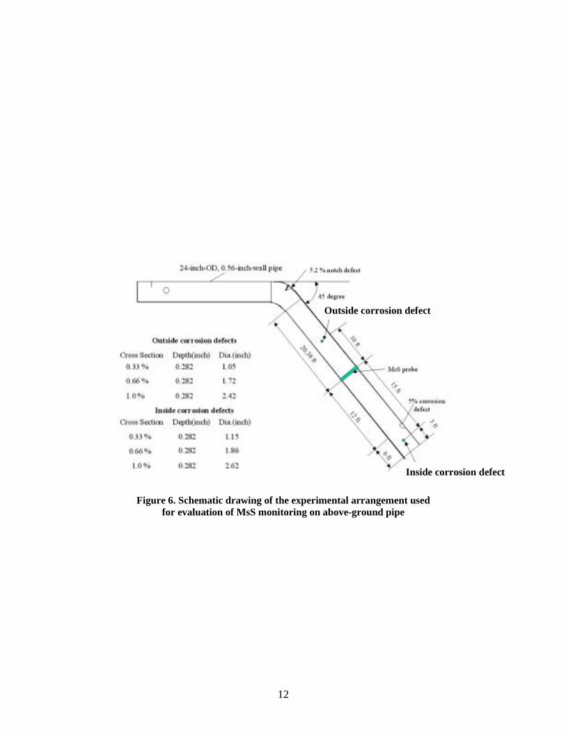
Figure 6. Schematic drawing of the experimental arrangement used for evaluation of MsS monitoring on above-ground pipe

Outside corrosion defect

Inside corrosion defect

13

(a)

(b)

Figure 7. Photograph showing (a) the topography and (b) replica of the intentionally placed 1% cross-sectional defects

14

MsS data were collected from the intentionally placed ID and OD defects. The OD

defects were on one side of the MsS sensor and the ID defects were on the other side. Figure 8

shows the actual inspection data collected from the pipe with no OD defect, with an OD defect

that is approximately 0.33% of the pipe wall cross section, with the OD defect increased to

0.66% of the pipe wall cross section, and finally with the OD defect increased to 1% of the pipe

wall cross section. This defect is approximately 3 m (10 feet) from the MsS. The 0.33% defect is

difficult to see in Figure 8, but the 0.66% and 1% defects can clearly be detected. The

preliminary monitoring data are shown in Figure 9 where the MsS inspection data collected prior

to placing defects in the pipe are used as the reference waveform. These data clearly show that

defects as small as 0.33% can be detected in the monitoring mode. The signals on the right side

of the last waveform in Figure 9 are caused by slight changes in temperature and the slight offset

in subtracting two large signals. In addition, when the amplitude of the signal that would

normally travel to the weld and the 5.2% notch is decreased because the signal is scattered by the

0.33%, 0.66%, and 1% defects, then the difference waveform between the reference where there

is no defect and the cases where the defect at 3 m (10 feet) increases from 0.33% to 1% would

yield a larger and larger difference in the signals observed after the defect at 3 m (10 feet). This

behavior is clearly seen in the difference data for the 0.33% and 1% defects. It is unclear why it

appears to be minimal in the 0.66% data difference waveform. Similar data are shown in Figure

10 with the video signals.

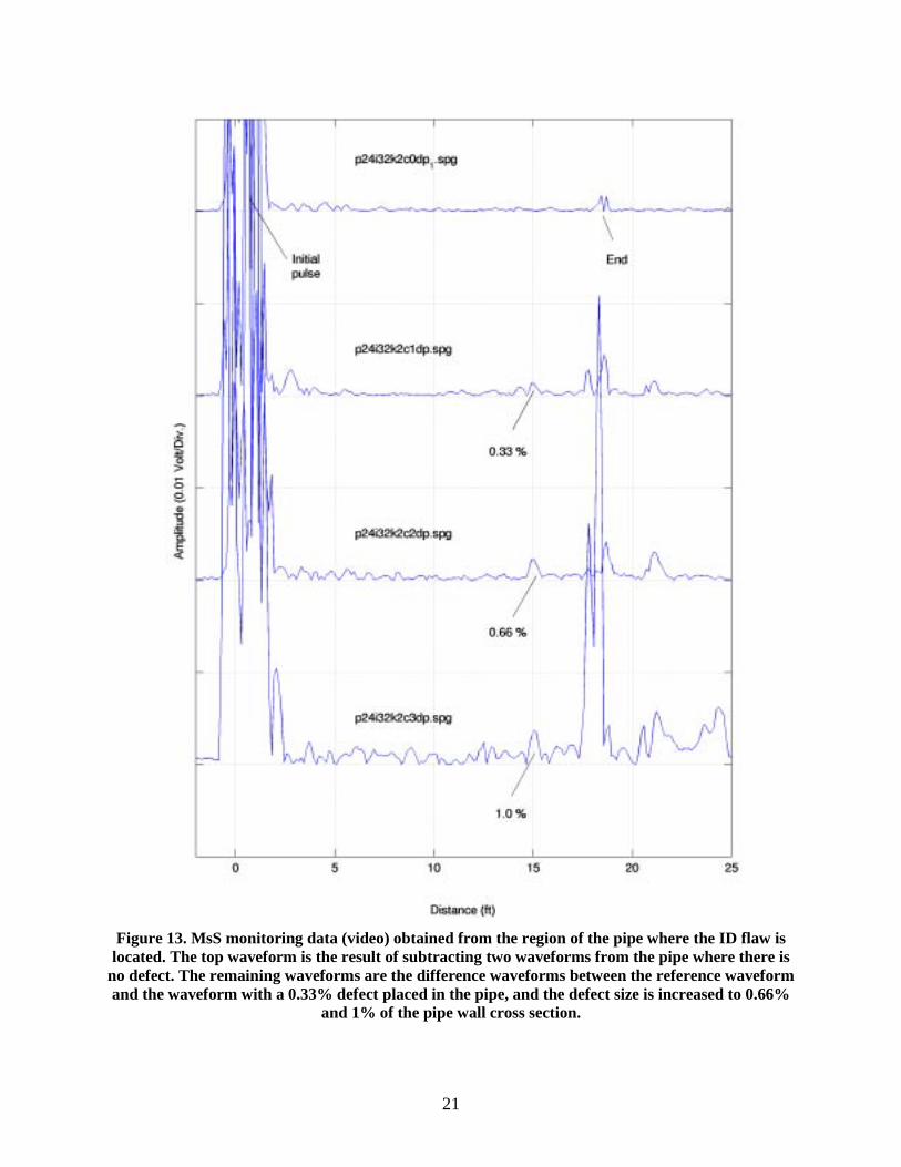
Similar results were obtained for the ID defects. The inspection data waveforms are

shown in Figure 11 and the monitoring (subtracted) waveform data are shown in Figure 12 and

Figure 13.

These data clearly showed that the MsS had the capability to detect small defects in

the monitoring mode in large diameter pipe. However, some questions about applicability to gas

transmission pipeline remained, including what effect bitumen coating might have on the signal,

and what would be the effect of burying the pipe.

To address the bitumen effect, a nickel strip was epoxied onto 406-mm (16-inch)-

OD, bitumen-coated pipeline as shown in Figure 14 that had a number of 1% defects at various

axial locations. Data were collected at 10 and 20 kHz guided wave frequencies. No data were

collected at higher frequencies because previous work [1] has shown that bitumen-coated pipe

15

would not effectively propagate 32-kHz waves. The experiments showed that 20-kHz guided

waves were not effectively transmitted. However, 10-kHz guided waves did appear to be

effectively propagated. Data were collected on this 406-mm (16-inch)-OD pipe after a 1% defect

was paced in the pipe approximately 3 m (10 feet) from the MsS. The data obtained show that a

1% defect could not be detected using the 10-kHz nickel foil probe at a distance of 3 m (10 feet

as shown in Figure 15. This indicates that bitumen-coated pipe is very difficult to inspect and

monitor using the present state of the art of the MsS technology.

16

Figure 8. MsS inspection data obtained from the region of the pipe where the OD flaw is located. The top waveform shows no defect. The remaining waveforms are from a 0.33% defect placed in

the pipe, and the defect size is increased to 0.66% and 1% of the pipe wall cross section.

17

Figure 9. Monitoring data (subtracted from the reference) obtained from the region of the pipe

where the OD flaw is located. The top waveform is the result of subtracting two waveforms from the pipe where there is no defect. The remaining waveforms are the difference waveforms between the reference waveform and the waveform with a 0.33% defect placed in the pipe, and the defect

size is increased to 0.66% and 1% of the pipe wall cross section.

18

Figure 10. MsS monitoring data (video) obtained from the region of the pipe where the OD flaw is located. The top waveform is the result of subtracting two waveforms from the pipe where there is

no defect. The remaining waveforms are the difference waveforms between the reference waveform and the waveform with a 0.33% defect placed in the pipe, and the defect size is increased to 0.66%

and 1% of the pipe wall cross section.

19

Figure 11. MsS inspection data obtained from the region of the pipe where the ID flaw is located. The top waveform shows no defect. The remaining waveforms are from a 0.33% defect placed in

the pipe, and the defect size is increased to 0.66% and 1% of the pipe wall cross section.

20

Figure 12. MsS monitoring data (subtracted from the reference) obtained from the region of the pipe where the ID flaw is located. The top waveform is the result of subtracting two waveforms from the pipe where there is no defect. The remaining waveforms are the difference waveforms

between the reference waveform and the waveform with a 0.33% defect placed in the pipe, and the defect size is increased to 0.66% and 1% of the pipe wall cross section.

21

Figure 13. MsS monitoring data (video) obtained from the region of the pipe where the ID flaw is

located. The top waveform is the result of subtracting two waveforms from the pipe where there is no defect. The remaining waveforms are the difference waveforms between the reference waveform and the waveform with a 0.33% defect placed in the pipe, and the defect size is increased to 0.66%

and 1% of the pipe wall cross section.

22

Figure 14. Photograph of the bitumen coated, 16-inch-diameter pipe

To address the effects of the MsS signal on buried pipe, a long pipe was

constructed from two 12.2-mm (40-foot)-long sections of 610-mm (24-inch)-diameter pipe

obtained from El Paso Corporation and welded together as shown in Figure 16.

23

Figure 15. Data showing that a 1% defect could not be detected

using the 10-kHz nickel foil probe at a distance of 10 feet flaw distance

24

Figure 16. Photograph of two 40-foot-long sections

of 24-inch-diameter pipe welded together

3.2.3 Laboratory Testing of MsS on Buried Piping

Even though the experimental results showed that inspection and monitoring of

bitumen-coated pipeline was difficult, work continued to determine whether the MsS could be

used on a buried pipeline and under buried pipeline conditions.

SwRI placed several MsSs on buried pipe section to evaluate the effects of the MsS

being buried. The 610-mm (24-inch)-OD, 24.4-m (80-foot)-long pipe (shown in Figure 16 prior

to burying and in Figure 17 after burying) was buried on the grounds at SwRI so that both ends

of the pipe were accessible. The MsSs were buried with the wire leads accessible aboveground

(as shown in Figure 18). The location of the MsS with respect to the welds and defects is

illustrated in Figure 19. MsS data using 20 kHz were collected from this pipe after it was buried.

MsS reference data were collected using the buried sensor before simulated corrosion was placed

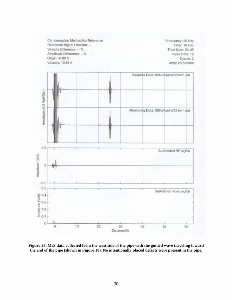
in the pipe. These data are shown in Figures 20 through 23. It is important to note that the data

shown in the two top waveforms in Figures 20 through 23 represent reference data taken within a

few minutes of each other. The respective difference waveforms should show very little

difference and indeed the difference waveforms are almost a straight line showing no difference

(except at the 0 point in the waveform). The amplitude difference at the 0 point of the waveform

is due to the fact that the initial pulse is saturated and differences of digitized saturated signals do

not accurately subtract.

25

Defects were placed in the buried pipe. These intentionally placed defects were

each approximately 1% initially [approximately 4.1 mm (0.1625 inch) deep by 62.2 mm (2.45

inches) in diameter]. The MsS data for one of the 1% defects is shown in Figure 24. The data

initially collected from the other 1% defect (from the west side of the pipe as illustrated in Figure

18) was lost due to a computer data acquisition failure. The 1% defect in the west side of the pipe

was increased to approximately 2% [approximately 4.1 mm (0.1625 inch) deep by 76 mm (3.0

inches) long] using 12 holes that measured 0.64 mm (0.025 inch) in diameter in a line and MsS

data were collected. These data are shown in Figure 25. These data clearly show that the MsS

technique can detect defects as small as 1 to 1-1/2%.

Figure 17. Photograph of the 24.4 m (80-foot)-long, 610-mm (24-inch)-diameter pipe

buried under approximately 0.6 m (2 feet) of soil

26

Figure 18. Photograph of one of the locations of an MsS bonded to the buried 610-mm (24-inch)-diameter pipe

Figure 19. Illustration of the buried 610-mm (24-inch)-diameter pipe showing the locations

of the MsS probes, the weld, and the intentionally placed simulated defects

West East

27

Figure 20. MsS data collected from the east side of the pipe with the guided wave traveling toward the end of the pipe (shown in Figure 18). No intentionally placed defects were present in the pipe.

28

Figure 21. MsS data collected from the east side of the pipe with the guided wave traveling toward the weld in the pipe (shown in Figure 18). No intentionally placed defects were present in the pipe.

29

Figure 22. MsS data collected from the west side of the pipe with the guided wave traveling toward the weld in the pipe (shown in Figure 18). No intentionally placed defects were present in the pipe.

30

Figure 23. MsS data collected from the west side of the pipe with the guided wave traveling toward the end of the pipe (shown in Figure 18). No intentionally placed defects were present in the pipe.

31

Figure 24. MsS data collected from the pipe with 1 percent of the total pipewall cross-section defect at 6 m (20 feet). It is difficult to visually detect any difference between the reference inspection data and the inspection data obtained from the pipe with the 1-percent defect. However, the difference

(subtracted data) clearly shows a signal at 6 m (20 feet).

32

Figure 25. MsS data collected from the pipe with 2 percent of the total pipewall cross-section defect at 6 m (20 feet). It is difficult to visually detect any difference between the reference inspection data and the inspection data obtained from the pipe with the 2-percent defect. However, the difference

(subtracted data) clearly shows a signal at 6 m (20 feet).

3.3 Optimization of the MsS Technology

The optimization of the MsS technology primarily dealt with how to mount the MsS to the

pipeline. A preliminary procedure for mounting the MsS onto the pipeline was developed and is

contained in Appendix 1. This procedure dealt with cleaning the pipeline, bonding the nickel

strips to the pipeline, placing and fixing the excitation coils, and covering the complete probe to

minimize damage during reburial of the pipeline.

33

Based upon the results obtained in the laboratory tests and the optimization of the sensor

for use on a buried pipe, it was believed that the technology was ready for evaluating on a

limited scale field test.

3.4 Field Tests

SwRI and Clock Spring® worked with El Paso Corporation to find a pipeline that could be

used to evaluate the MsS monitoring technology. Two pipelines were located and the field tests

were conducted as described in the following sections.

3.4.1 Field Test Conducted Near Cleveland, Texas

(1) Discussion

A low-lying section of buried, 610-mm (24-inch)-OD, bitumen-coated gas

pipeline (laid in 1944 and presently owned by El Paso Corporation) located approximately 13

miles north of Cleveland, Texas was excavated on May 5, 2003 as part of a plan to re-evaluate an

internal corrosion defect found in 1998 using a magnetic flux leakage pig. The corrosion defect

was located in a low spot in the pipeline, and there was concern about potential corrosion

growth. The plan called for inspection using X-ray and UT thickness measurements. El Paso

Corporation allowed SwRI to work with Clock Spring® to place an MsS on the pipeline to

evaluate the sensor’s capabilities to monitor corrosion growth in buried pipeline.

A section of the pipe approximately 7.6 m (25 feet) long was excavated (as

shown in Figure 26). The weld was located by the El Paso crew and marked as a landmark. The

corrosion defect was approximately 16 feet from the weld. A 2.1-m (7-foot)-long section of wax-

based coating was removed for X-ray and UT thickness measurement testing (as illustrated in

Figure 27). The topside of the pipe was wrinkled at approximately 0.6 m (2 feet) increments. The

wrinkles were the result of the technique used for many years to bend the pipe in the field;

however, this practice is no longer used. There was some concern about the effect the wrinkles

might have on the MsS results. A 0.3-m (1-foot)-long section of bitumen coating was removed

and the pipe was sandblasted so that the MsS probe could be installed.

34

Figure 26. Photograph of the pipe excavated at the Cleveland site

showing the location of the MsS coil and bend rings

Figure 27. Photograph and diagram showing the MsS ribbon coil and pipe

The MsS (as shown as a yellow band in Figure 25) transmitted T-waves into

each direction of the pipeline and received T-waves reflected from the defects. The signal

amplitudes and arrival times were investigated to measure the defect size and its location,

respectively. The MsS, consisting of two bonded 2.5-mm (0.10-inch)-thick nickel strips and an

electric coil wrapped on it, were used to inspect and monitor defects that caused the cross-

sectional area change.

Several observations were made during the process of placing the MsS

nickel strips on the pipeline. First, the pipeline was at a temperature of approximately 4°C (40°F)

when it was excavated. The air was very warm and humid (estimated to be approximately 29.5°C

(85°F) and 70-80% humidity). As soon as the pipe coatings were removed, moisture began to

condense on the pipe surface. It was necessary to dry the pipe surface in order to bond the nickel

strips onto the pipeline. The El Paso crew used a propane burner to remove the wax coating and

also suggested using this approach to dry the pipe in the area where the MsS nickel strips were to

be placed. The nickel strips were successfully bonded onto the pipeline, and because it was late

in the day, the strips were left in place overnight.

0ft

Coated region

24-inch-OD, 0.25-inch-wall pipe MsS probe

Weld

10.7ft 15.2 ft 22.2 ft

35

MsS data were taken the following morning. Figure 28 (a) and (b) show the

20-kHz MsS data taken by directing the T-waves toward the uncoated region (toward the defect)

and the weld, respectively, from the MsS probe positioned approximately 3.3 m (10.75 feet)

from the weld. Signals from the weld and boundaries of coating in the sample were indicated. A

randomly distributed noise-like signal appeared after the initial pulse in both directions,

indicating the inside of the pipe had a high level of generalized internal corrosion on both sides

of the MsS. Similar MsS data were obtained from a pipe that was heavily corroded on the outside

[1]. Figure 29 is a photograph of the heavily surface-corroded section and the location of the

MsS probe. The MsS data in Figure 30 clearly show the signal difference between the good

surface between W5 and W4 and the heavily corroded section between W4 and W2.

Figure 28. 20-kHz MsS data acquired from excavated bitumen-coated pipeline: (a) with wave

directed toward the uncoated region; (b) with wave directed toward the closer weld

36

Figure 29. Photograph showing MsS probe installed

on pipe having a heavily corroded section

Figure 30. MsS guided wave data acquired from a natural corrosion pipe sample

37

Since the guided wave propagates uniformly with the same wave front

through the pipe wall cross-sectional area, generalized corrosion on either the outside or inside

surface of the pipe highly attenuates the propagating T-wave by reflecting and scattering

randomly distributed noise-like signals. If the MsS had been buried with the pipeline, the

initiation and growth of generalized corrosion could have been monitored by observing the

appearance and increase of randomly distributed noise-like signals. However, based upon the

results of the X-ray and UT thickness measurements and the preliminary results obtained with

the MsS, the decision was made to remove this section of pipe. Therefore, this test site was no

longer acceptable for evaluating the MsS technique for pipeline monitoring. However, the

condition of the pipe did show the need for a monitoring technique such as the MsS. If the MsS

could have been put in place and the pipeline had an acceptable corrosion level, then the MsS

could be used to monitor the corrosion growth without having to expose the pipe.

The corroded pipe section was cut out of the line and photographs were taken of the

opening. These photographs are shown in Figures 31 through 34.

Figure 31. Inside surface of pipeline showing major internal corrosion

38

Figure 32. Another view of the inside surface of the pipeline

showing major internal corrosion

Figure 33. Photograph of removed pipe

39

Figure 34. Photograph of replacement pipe before burying

(3) Conclusions of the Cleveland Field Test

A 20-kHz, torsional-mode, MsS-generated T-wave was capable of

inspecting 610-mm (24-inch)-OD, bitumen-coated gas pipelines. Based upon the MsS data

obtained, internal generalized corrosion was predicted because of the randomly distributed noise-

like signals and very high attenuation observed. It is believed that if the MsS probe had been

buried with the pipeline as a monitoring device, the initiation and growth of generalized

corrosion could have been monitored by observing the appearance and increase of randomly

distributed noise-like signals.

Practical lessons for applying the MsS to the pipeline were learned during this field test.

First, water will condense on the outside surface of cold, buried pipe if the temperature and

humidity conditions permit. Special attention will be required to dry the pipe surface prior to

bonding the nickel strip. Second, nickel strips can be successfully bonded to a buried pipeline.

In general, it is believed that this field test showed the potential for the MsS monitoring

technology, but another test was needed where the MsS can be buried for a long period to better

demonstrate the potential of the technology.

40

3.4.2 Field Test Conducted at El Paso Corporation Near El Paso, Texas

(1) Discussion

For the field test, the MsS was installed on a buried gas transmission

pipeline that was 762 mm (30 inches) OD, 11.4 mm (0.45 inch) thick, and coal-tar-enamel

coated. The installation was made on the El Paso Corporation’s Line 1600 at a location near

Chamberino East Lateral in El Paso, Texas. The installation location was on the west side of the

road crossing approximately 4.9 m (16 feet) from the end of the casing pipe of the line. This

section of pipeline was known to contain several external corrosion defects from the results of

Tuboscope Vetco Pipeline Service, Inc. in-line inspection (ILI) test conducted on April 9, 2002

and, therefore, was selected for monitoring in this field trial.

A team from SwRI installed the MsSs and took initial test data during

August 18-19, 2003. A crew from El Paso Corporation provided the site support that was needed

for installing the MsSs. This support included preparation of a bell hole and removal of the

coating; after the sensor was installed, the pipe was recoated and the site was restored.

A section of pipeline approximately 2.1 m (7 feet) long was excavated and

exposed at the west side of the road crossing and an approximate 0.3-m (1-foot)-wide strip of

bitumen coating was removed around the pipe to mount the MsSs. The depth of the soil cover at

the MsS installation location was measured to be approximately 10 feet. In the region where the

coating was removed, two 0.25-mm (0.01-inch)-thick and 15.9-mm (0.625-inch)-wide nickel

strips separated by 40.6 mm (1.6 inches) were bonded to the pipe around its circumference by

using Devcon 5-minute epoxy. Fourteen turns of # 22 gauge wire were wound over each nickel

strip. Figure 35 shows a photo of the MsSs installed on the pipeline. The remaining length of

each wire was twisted and connected to a waterproof box tied to a pole approximately 4.9 m (16

feet) from the MsS location as shown in Figure 36. After the MsS installation, the MsSs and the

coating-removal area were covered with a thick tape to prevent water intrusion and offer

protection from corrosion. Also, the twisted pairs of wire between the MsS and the aboveground

box were placed in a flexible steel tube for protection during the refilling process of the bell hole

and the long-term monitoring period.

41

To identify the locations of the MsSs, the configuration of the pipeline at

the road crossing is schematically illustrated in Figure 37, including the locations of known

geometric features and known defects found from the ILI results. The distance between the

center of two MsSs and the nearest weld (No. 2827) was 0.22 m (0.73 feet). The corrosion

defects found from the ILI results are indicated as A1 through A5 and their characteristics are

summarized in Table 3. It should be noted that the detection sensitivity determined during

laboratory tests on buried pipe was on the order of 1.5 to 2% of the pipe wall cross section. The

defects listed in Table 3 were much smaller. These small defects can be detected by pigs, but

monitoring could detect defects that are larger but still acceptable for continued pipeline

operation, then the monitoring technology would provide an inexpensive alternative to pigging

(if it is possible at all).

Figure 35. MsS installed on the 762-mm (30-inch)-OD gas transmission pipeline

Figure 36. Photograph showing a waterproof box after the site was restored

42

Figure 37. Configuration of the pipeline at the road crossing. The locations

of the MsS and distances to the known geometric features in the line are indicated.

Table 3. Known Corrosion Defects Found from Tuboscope’s ILI Results

After the sensor installation and restoration of the excavated site on

August 18, 20-kHz MsS data were acquired by transmitting the T-wave in the road crossing

direction and detecting signals reflected back from defects in that side of the pipeline. The data

acquisition process was repeated again the following day, approximately 15 hours after the time

of the first data acquisition. Because of high attenuation in bitumen-coated and buried pipelines

[1], the returned signals were very weak. To detect weak signals, a very high receiver gain (56

dB) and a fine input voltage range (100 mV) were used for data acquisition. In comparison,

typical gain and input voltage range used for aboveground piping inspection is 20 db dB and 500

mV. The signal amplification used in this test was, therefore, 315 times higher than that typically

used for aboveground piping inspection.

Mark of Anomaly

Distance from MsS probe (Foot)

Depth (%)

Length (Inch)

Location Cross-Sectional Area (%)

A1 15.36 15 3.1 External 0.5 A2 15.72 15 1 External 0.2 A3 31.81 24 3.2 External 0.8 A4 34.86 24 1.5 External 0.4 A5 36.53 19 2.9 External 0.6

43

Figure 38 (a) and (b) shows the data acquired on August 18 and 19,

respectively. The locations of welds (Nos. 2825 and 2826) are indicated in the figure as the

vertical dotted lines. As shown, the two sets of data were approximately identical, indicating that

the installed MsSs were stable and repeatable.

Figure 38. 20-kHz MsS data acquired from the 762-mm (30-inch)-OD gas transmission line: (a)

after restoration of the line and (b) 15 hours after restoration of the line Because of the high attenuation in the bitumen-coated and buried lines, no

detectable signal was detected from weld No. 2826 at approximately 3.9-m (12.9-feet) distance

from the MsS. Also, signals from the known corrosion defects were not observable in the data

since they were too far away from the sensor location to be detectable.

Because of the high signal amplification, the background electrical noise

(those signals occurring before the initial pulse or over –1.3 to 0 m (–5- to 0-feet) distance in the

plot) was noticeable in Figure 38. Signals that exceeded the background noise level were

observable only for up to approximately 3-m (10-feet) distance in the data because of the high

wave attenuation.

44

At high amplifications such as those used in this test, detectable signals are

produced from the MsS system after the excitation of the initial pulse. The signals over 3-m (10-

feet) distance in Figure 37 are, therefore, most likely to be those produced from the MsS system

and not from any actual anomalies in the pipeline itself. This interpretation would indicate that

the signals seen past 3 m (10 feet) were from electronic noise, not defects. This interpretation is

consistent with Tuboscope’s test results that showed no defect indications in the pipe section

between welds 2826 and 2827 on which the MsS was installed. A second data collection was

conducted on September 9, 2003. The comparison of the initial data and the most recent data is

shown in Figure 39. As expected, no significant difference in signal was detected. It is believed

that perhaps changes will occur within a year, and the setup was left in place so that data could

be collected again in approximately 1 year.

Figure 39. 20-kHz MsS data acquired from the 762-mm (30-inch)-OD gas transmission line:

(a) 15 hours later after restoration of the line and (b) 22 days later after restoration of the line

Tracking the performance of the installed MsSs and the structural condition

of the pipeline over an extended period of time requires a reliable reference signal in the data.

Frequently, signals from welds adjacent to the MsS serve as the reference signals in the long-

term monitoring process. Because no detectable weld signals were seen in the initial data means

45

that there was no reliable reference signal available for monitoring use and, consequently, long-

term monitoring of the pipeline using the installed MsS in this field trial would be difficult to

achieve.

In hindsight, the following would have helped to achieve long-term

monitoring:

(1) When reference signals are lacking, install two sets of sensors

separated by some distance [for example 3 m (10 feet)] to allow the

detection of a transmitted signal in the pitch-catch mode. Then, use

the transmitted signal as the reference.

(2) The wave attenuation in the bitumen-coated and buried pipelines

increases significantly with the depth of soil cover as found in

previous EPRI projects [2]. Therefore, the attenuation at the encased

section at the road crossing, where the pipe should have no soil

cover around it, should be much lower than in the other areas of the

pipeline that are covered with soil. Because of the significantly

lower attenuation in the encased section, the long-term monitoring

of this section and any changes in the known existing defects could

have been achievable with the MsS installed just outside of the end

of the casing pipe. It is critical to install the MsS in the correct

location.

(2) Conclusions from El Paso Pipeline Data

MsS sensors were installed on a 30-inch-diameter, bitumen-coated, buried

gas transmission line for long-term monitoring evaluation purposes. Because of the high wave

attenuation in the pipeline, detection of signals from a nearby weld at approximately 3.9-m

(12.9-feet) distance or other known defects further away was difficult to achieve with the

installed MsS. Although periodic testing of the line using the installed sensor is planned, tracking

of the long-term MsS performance and the monitoring of the pipeline is expected to be difficult

due to the lack of detectable signals from the MsS location.

46

3.5 Lessons Learned

(1) Reference signals must be established for monitoring applications when dealing

with pipe that has been buried for many years and that most likely has a significant

amount of generalized corrosion. Approaches that could be used for obtaining

references are installing two sets of MsSs separated by appropriate distances to

allow the detection of the transmitted signal or installing the MsS at a location that

allows the detection of the nearest weld.

(2) Selection of MsS location is critical.

(3) Good planning with accurate site information is required.

47

4.0 CONCLUSIONS

As a result of this work, the following conclusions were reached.

First, laboratory tests were conducted at the SwRI facility on several different types of buried

pipe of various lengths as follows:

(1) A schedule 60 pipe with no corrosion prevention coating that was 610 mm (24 inches) OD,

18.3 m (60 feet) long, had a 45-degree elbow, and tested in air;

(2) A schedule 40 pipe with a bitumen coating that was 406 mm (16 inches) OD, 9.15 m (30

feet) long, and tested aboveground; and

(3) A schedule 40 pipe with no coating that was 610 mm (24 inches) OD, 24.4 m (80 feet)

long, tested in air, and buried.

Second, MsSs, consisting of T-wave coils with a ferromagnetic nickel foil (T-wave sensor), were

developed and mounted to the test pipes. The prototype waveform differential algorithms,

previously developed by SwRI to detect small geometric differences in MsS waveforms, were

used to collect data during the laboratory evaluation. Initial (baseline) data were collected and

used as a reference before artificial defects were placed in the pipeline. The artificial defects,

consisting of ground-out regions, were placed in the inner and outer pipewall surfaces to

simulate corrosion pits. Signal-processing algorithms that perform a comparison of reference

data and the data after defects were introduced were used, and an approximate defect detection

sensitivity as a function of defect size, steel attenuation, and pipe coating was determined.

Third, twenty different epoxies were evaluated, and the Devcon 5-minute epoxy was found to be

the easiest to apply, most reliable, and, to date, robust. Nickel foil sensors bonded with the

Devcon 5-minute epoxy on a pipe exposed to an outside pipeline environment for more than 2

years are still fully functional.

Fourth, for buried pipes that were not coated with bitumen, the defect detection sensitivity was

approximately 1% of the total pipe wall cross section.

48

Fifth, although no evidence was developed, it is estimated that the MsS defect detection

sensitivity for bitumen-coated pipes would be on the order of 2-3% defects through an inspection

range of approximately 3-6 m (10-20 feet).

49

5.0 REFERENCES

[1] Torsional Guided Wave Examination of Buried Piping. EPRI, Palo Alto, CA: 2002. 1006308

[2] H. Kwun, C. P. Dynes, and S. Y. Kim. “Evaluation of the Magnetostrictive Sensor (MsS) Technique for 24-inch Gas Pipeline Inspection.” Southwest Research Institute® sponsored by the Gas Research Institute (GRI).

A-1

6.0 APPENDIX

PRELIMINARY MAGNETOSTRICTIVE SENSOR (MsS) INSTALLATION

PROCEDURE FOR GAS PIPELINE MONITORING

Introduction

Southwest Research Institute was funded by the Department of Energy (DOE) under the

National Energy Technology Laboratory (NETL) program to evaluate the magnetostrictive sen-

sor (MsS) monitoring technology on buried pipeline. The purpose of the effort was to demon-

strate that the MsS can successfully monitor changes in corrosion found at the low spots of a gas

transmission pipeline. To accomplish this goal, laboratory work on various sizes of pipe was

conducted to (1) demonstrate that small changes (on the order of 1 percent of the pipeline wall

cross section) could be detected and (2) optimize the MsS probe for use on a buried pipeline. In

addition, two MsS probes were mounted onto a 24-inch pipeline approximately 80 feet long and

then buried.

Application Guideline

As part of this project, a guideline for applying the MsS sensor to a pipeline was developed. The

following provides a guideline for the application of MsS sensors on large-diameter piping for

long-term monitoring. Each application may have some special circumstances that require

slightly different techniques, but this procedure provides a basic guideline for application of the

MsS to the pipeline.

1. Access to the pipeline is required. For the case of a buried pipeline, a bell hole large enough for two men to work in and providing at least a 12-inch clearance below the pipe will be needed. The application work involves wrapping epoxy-coated nickel strips around the pipe surface as well as hand-winding electrical coils, so a 3-foot area on each side of the pipe is needed to allow a person to get down below as well as above the pipe. An excavation large enough and deep enough to place the pipe at mid-chest level with room to bend down would be ideal. If the application is aboveground requiring scaffolding, then again placing the structure to allow access to both sides as well as top and bottom is necessary.

2. Preparation of the pipe surface requires removal of insulation or coatings such as bitumins, plastic, or rubber. Loose material such as rust, scale, dirt, or loose paint should be removed using approved tools such as wire brush. Tightly adhering paint is acceptable and does not have to be removed. There is no need for polishing the pipe surface. A minimum surface

A-2

consisting of 12 inches along the pipe axis and completely around the pipe should be cleaned.

3. Application of nickel will usually require the use of various lengths of nickel in lieu of a continuous piece of nickel. For example, a 24-inch-diameter pipe requires more than 6 feet of nickel (πd or 24 times 3.1417 = 75 inches) to make one complete wrap around. These lengths of nickel foil can become unmanageable when trying to coat the foil with epoxy and applying it to a pipe surface smoothly without gaps or air pockets. Dirt from the excavation is also a problem, so shorter lengths are the best practice. The application of shorter lengths will require more time, because sensor application to the pipe is critical to making the MsS monitoring technology work. Bonding shorter lengths of nickel to the pipe provides for easier repair in the case of a bad application of the nickel foil. The nickel used is approx-imately 5/8 inch wide and 0.010 inch thick. Two strips of nickel are applied to the pipeline circumference with center-to-center spacing of 1.6 inches. The two strips are necessary for unidirectional switching operation of MsS. The spacing between the strips coincides with the 20-kHz operating frequency found to be optimum for buried pipe. Aboveground piping would usually require a different spacing/frequency combination.

4. The nickel must be applied smoothly with no gaps on the side, no twist in the nickel, and no air pockets in the bond line. It must also be aligned around the pipe so that the ends of the nickel strips meet cleanly, without overlap or misalignment. A visual guide helps to keep the nickel in alignment. A good practice is to use a tape measure to mark a point along the axis of the pipe from a reference point. Then mark a line on the pipe completely around the cir-cumference. This will be the edge of one of the nickel foils.

5. The epoxy proven to be the best for this application is Devco 5-minute epoxy, No. 14250. It mixes to a thick, smooth liquid that is easily spread on the nickel, and it allows sufficient time before cure to apply it to the nickel and place the nickel on the pipe. The epoxy is mixed and spread using a tongue depressor.

6. Spread the epoxy on the nickel, not on the pipe surface. Use tape (such as 3M electrical tape, No. HD 0242 04) to tape down the foil, and apply even pressure to the nickel while the epoxy cures. Leave the tape in place after the epoxy cures because trying to remove the tape often breaks the epoxy bond and ruins the application. Figure 1 shows the tape wrapped around the two nickel strips with their outline marked with a pen.

7. Magnetize the nickel strips using two small horseshoe magnets taped together at the proper spacing so that both nickel strips are magnetized simultaneously. The magnets are placed on top of the nickel strips and passed along the nickel strips in a smooth, even pace. The poles of the magnet are protected with tape, and a tissue is used to allow the magnets to slide smoothly along the nickel strips. Three to five passes around the circumference are required. It is important while magnetizing the strips to keep a continuous motion around the pipe. To do this in the bell hole, it is best to have one person on each side of the pipe so that they can pass the magnet smoothly from one to the other. The magnet is smoothly lifted off the nickel to complete the magnetization process.

8. Validate good bonding of the nickel foil to the pipeline by using coil adapters and ribbon cable to generate a magnetostrictively induced guided wave into the nickel and observing

A-3

the amplitude of the wave reflected from a pipeline feature such as a girth weld. If the signal is acceptable, then the application of the nickel foil has been validated. If the signal is not acceptable, then the nickel must be removed and the application process repeated using new nickel foil. (NOTE: Nickel foil removed from the pipe is damaged and should not be used again due to stresses set up in the nickel foil during the removal process.)

Figure 1. Photograph showing tape wrapped around the two-nickel strips

with their outline marked with a pen

9. Remove the temporary coils and place double-sided tape over the nickel foil once good guided wave results have been observed and recorded. The reason for marking the edge of the nickel with a pen is to aid in the placement of the tape directly over the nickel foil. Using #22 awg insulated wire, carefully wrap a coil of 16 turns around the pipe. Double-sided tape placed over the nickel foil is used to hold the wire in place while the 16 turns are being made. Mark one end of the wire with tape prior to beginning the wire wrapping process. Leave enough wire free at both the beginning and the end of the coil to extend out of the excavation to the eventual test box. It is good practice to use different colored wires for the two coils so that the two coils can be properly identified when connected into the test box. (NOTE: Always wind the coils in the same detection. A mix-up here could mean you are looking in the wrong direction later.) Once the two coils have been wound around the pipe, twist the ends of the coil wires together so that coming out of the excavation are two twisted pairs of wires of different colors with a tape tag indicating the first turn wire. Fig-ure 2 is a photograph of the coils wound on the pipe showing a yellow vinyl duct tape used to cover the windings of one coil while the second coil is held down with double-sided tape. Then, the layer of protective tape is placed over the nickel strip and electrical coil (Figure 3).

A-4

Figure 2. Photograph of the coils wound on the pipe showing yellow vinyl duct tape used to cover

the windings of one coil while the second coil is held down with double-sided tape

Figure 3. Protective tape coating over nickel strip and electrical coil

A-5

10. Run the twisted-pair coil leads through plastic conduit up to an outdoor “J” box normally used for 110-volt outdoor electrical installation. Either a metal or plastic outdoor electrical box is acceptable.

11. Solder the leads into a LEMO panel mount two-pin connector. The part number for this connector is EGG 0B-302 CLL. Heat shrink should be used to insulate the leads on the back of this connector. The first turn lead, marked with tape as described earlier, is soldered into the pin, which has a white half-circle mark on the back of the connector. Proper installation of the wire into the connector is important so the direction the sound wave is traveling can be known, so that when a defect is observed in the data, the direction and distance from the sensor can be accurately measured off above the buried pipe. A handy rule of thumb is that the sound travels from the channel one coil to the channel two coil when the system is in the positive mode. Positive mode is when the transmitter switch is positive. The junction box and connections used in monitoring are shown in Figure 4.

12. Backfill of the bell hole should be made only after all connections are made and the system is tested in its completed condition. Care should be taken in the backfill, and only sand should be used around the coils. Damage can occur if the coils are struck with tools or rocks, and caution should be taken in dumping sand into the hole around the coils.

Figure 4. Photograph of the junction box showing the connectors that

are connected to the MsS instrument for collecting MsS data