Expert Systems with Applications 39 (2012) 7110–7120

Contents lists available at SciVerse ScienceDirect

Expert Systems with Applications

journal homepage: www.elsevier .com/locate /eswa

Monitoring industrial processes with SOM-based dissimilarity maps

Manuel Domínguez a,⇑, Juan J. Fuertes a, Ignacio Díaz b, Miguel A. Prada a, Serafín Alonso a, Antonio Morán a

a Universidad de León, Grupo de Investigación SUPPRESS, Instituto de Automática y Fabricación, Escuela de Ingenierías, Campus Universitario de Vegazana, León 24071, Spainb Universidad de Oviedo, Área de Ingeniería de Sistemas y Automática, Campus de Viesques, Edificio Departamental 2, Gijón 33204, Spain

a r t i c l e i n f o a b s t r a c t

Keywords:Self-organizing mapBatch monitoringIndustrial processesInformation visualizationData-based monitoring

0957-4174/$ - see front matter � 2012 Elsevier Ltd. Adoi:10.1016/j.eswa.2012.01.033

⇑ Corresponding author. Tel./fax: +34 987291694.E-mail addresses: manuel.dominguez@unileon.es

unileon.es (J.J. Fuertes), idiaz@isa.uniovi.es (I.(M.A. Prada), saloc@unileon.es (S. Alonso), a.moran@u

Today’s large scale availability of data from industrial plants is an invaluable resource to monitor indus-trial processes. Data-based methods can lead to better understanding, optimization or detection of anom-alies. As a particular case, batch processes have attracted special interest due to their widespreadpresence in the industry. The aim of monitoring, in this case, is to compare different runs or implemen-tations of a process with the baseline or normal operating one. On the other hand, visual exploration toolsfor process monitoring have been a prolific application field for self-organizing maps (SOM). In this paper,we exploit data-based models, obtained by means of SOM, for the visual comparison of industrialprocesses. For that purpose, we propose a method that defines a new visual exploration tool, called dis-similarity map. We also expose the need to consider dynamic information for effective comparison. Themethod is assessed in two industrial pilot plants that implement the same process. The results arediscussed.

� 2012 Elsevier Ltd. All rights reserved.

1. Introduction

A better understanding and knowledge about the nature andperformance of industrial processes is increasingly necessary tomeet the strict requirements of productivity and quality of today’sindustry. Most industrial processes include ingredients such aslarge number of variables, nonlinearities, degradation due to wearor aging, etc. These characteristics increase the complexity of mod-els that are required to be accurate enough to suggest improve-ments or to detect significant changes that lead to an impact onquality or productivity. Therefore, model-based approaches mightnot be easy to implement in large and complex industrial pro-cesses. For this kind of processes, we usually lack of reliable orprecise models, and knowledge about the nature of faults is seldomexpressed in rationalized ways, such as mathematical models, orwell-defined sets of rules or procedures for diagnosis.

Batch processes (Nomikos & MacGregor, 1995), characterizedby its finite nature and non-steady-state behavior, are one kindof process that has strong requirements with regard to monitoring.The aim, in this case, is to guarantee that the production of thespecified product is consistent among runs. The usual approachto address this problem is multivariate statistical process control,which models the process using data obtained when the processis in the normal operating condition. This approach can be framed

ll rights reserved.

(M. Domínguez), jj.fuertes@Díaz), ma.prada@unileon.esnileon.es (A. Morán).

as novelty detection (Chandola, Banerjee, & Kumar, 2009). Noveltyand change detection approaches are well suited to those problemswhere the set of potential faults is unknown or even unmanage-able. They rely on computing and assessing the differences of thecurrent process behavior with respect to the expected (normal)behavior. They generally use statistics (Markou & Singh, 2003) tocompute thresholds that reveal significant changes on one or moreprocess variables, which might facilitate early detection of faults.The set of involved variables might also be analyzed or classified(Gertler, 1998) later using prior knowledge about the faults.Indeed, typical classification approaches are difficult to conceivein process monitoring, since they require training data under allpossible fault conditions, which are often unavailable.

On the other hand, a large amount of non-rationalized and/orimprecise knowledge, built upon the experience of the staff thatspent a huge number of hours of observation and process supervi-sion, might be available. Information and data visualizationtechniques (Keim, 2002) are often very efficient approaches in suchcontexts. Visualization allows to exploit subtle forms of knowledgeas well as to take advance of the human ability to identify complexpatterns in a quick way and without taking resources to higherfunctions related to reasoning process. This makes visualizationapproaches very adequate ways to deal with unstructured knowl-edge typical in the analysis and monitoring of complex industrialprocesses such as batch processes.

Self organizing map (SOM) (Kohonen, 2001) has been success-fully applied as a data visualization tool in many fields (Kohonen,Oja, Simula, Visa, & Kangas, 1996), including process monitoring(Alhoniemi, Hollmén, Simula, & Vesanto, 1999; Domínguez,

M. Domínguez et al. / Expert Systems with Applications 39 (2012) 7110–7120 7111

Reguera, Fuertes, Díaz, & Cuadrado, 2007; Hollmén, 1996). It hasalso proven to be a powerful technique for novelty detection(Ypma & Duin, 1997). We present in this work a method that usesself-organizing maps to visualize the dissimilarities between twoplants implementing the same batch process or, alternatively,two different runs of the same plant.

This paper is structured as follows: in Section 2, the self-orga-nizing maps and its previous applications to visualization arereviewed briefly. The proposed method is described in Section 3.The experimental architecture is explained in Section 4, whereasSection 5 presents the experiments and results. Finally, the conclu-sions are exposed in Section 6.

2. Self-organizing maps for visualization

The self-organizing map (SOM) (Kohonen, 1990, 2001) is a neu-ral network that allows to produce a smooth nonlinear orderedmapping from a high-dimensional input space X � Rn onto alow-dimensional visualization lattice V � Rd – typically 2D forvisualization. The low-dimensional space captures the latent struc-ture of the data in the input space, preserving the topology previ-ously defined in the lattice. The SOM algorithm is based on anunsupervised and competitive learning algorithm. Each neuron orunit i of the SOM is represented by the coordinates gi of the nodesof a regular 2D lattice in V and by a weight vector (codebook vec-tor) mi in X . The neurons are connected to the adjacent onesaccording to a neighborhood relation that sets the map topology,usually rectangular or hexagonal. During training, the SOM latticefolds in order to fit the input data sets, and the n-dimensional coor-dinates mi of the neurons are updated so that a larger number ofneurons gather in areas with a higher density of data. The neuronsdivide the space into a finite collection of Voronoi regions.

The original SOM training algorithm (Kohonen, 2001) com-putes, at each step, all the distances between the training vectorx and the codebook vectors mi. The unit with the shortest distanceto the input vector is called best matching unit (BMU) and it is de-noted as c. The weights of the unit mc, along with the weights of itsneighbors, are updated to approximate the training data, followinga competitive-cooperative scheme,

c ¼ arg minifkx�mik2g ð1Þmiðt þ 1Þ ¼ miðtÞ þ aðtÞhciðtÞ½xðtÞ �miðtÞ� ð2Þ

where k�k is the distance, usually Euclidean, x(t) is the input vectorof the training data set at time t, hci(t) is the neighborhood functionaround the winner unit c and a(t) is the adaptation coefficient attime t. The neighborhood function depends on time and distancefrom unit i to the winner neuron c. It defines the influence area ofthe input sample in the SOM:

hciðtÞ ¼ exp � dðgc; giÞ2rðtÞ2

!ð3Þ

where gc; gi � V are the node positions of units c and i in the SOMlattice, d(�, �) is a distance metric defined in V and r(t) is the neigh-borhood kernel width. The training is usually done in two stages. Inthe first stage, relatively large initial values of learning rate coeffi-cient a (t) and neighborhood kernel width r(0) are used to favor aproper ordering. In the second stage, both the learning rate andthe neighborhood kernel width decrease to favor dataapproximation.

The batch version of the SOM training algorithm is substantiallyfaster. At each training step, the indices of all the winning units foreach sample xj are obtained and the weight vectors which partitionthe data set are calculated:

cj ¼ arg minifkxj �mikg

miðt þ 1Þ ¼Pn

j¼1hcjiðtÞxjPnj¼1hcjiðtÞ

ð4Þ

where cj is the index of the BMU of sample xj.The SOM provides powerful ways of visualization, since it cre-

ates a smooth nonlinear mapping from a high dimension to alow dimension visualization space (Himberg, Ahola, Alhoniemi,Vesanto, & Simula, 2001). Any meaningful scalar property of theprocess pi that can be evaluated for every unit i in the input spacecan be represented in the visualization space using a pixel – or anykind of glyph – centered at position gi and having a color value cor-responding to pi in a given color scale. For regular lattices, this pro-duces the SOM planes. Each SOM plane represents the distributionof a meaningful property of the process for all the process states bymeans of a colored image. Moreover, since all planes are obtainedin the same way, all images present information in a consistentway, that is, planes can be compared and explored concurrently– as weather maps of a same country – allowing to merge differentkinds of knowledge about the process, that range from planesmerely representing the process variables or measurements forthe different states – the well known component planes (Tryba,Metzen, & Goser, 1989) – to more elaborated types of knowledge,such as cluster information – u-matrix – (Ultsch & Siemon, 1990),model-based knowledge – model maps – (Díaz, Cuadrado, & Díez,2004), rule-based knowledge – fuzzy maps – (Cuadrado Vega,Díaz Blanco, Diez González, Obeso, & González, 2001), local corre-lation information – correlation maps – (Díaz & Hollmén, 2002) andmore recently maps showing the dynamic response (Díaz, Domín-guez, Cuadrado, & Fuertes, 2008; Fuertes et al., 2010).

3. Dissimilarity maps

3.1. Visual comparison of industrial processes

In the introduction, we discussed the suitability of visualizationmaps, which enable a human supervisor to monitor an industrialprocess to check if its behavior corresponds to the normal operat-ing condition.

This section describes the proposed method, which comparesdifferent runs or implementations of an industrial process in orderto obtain the existing deviations between them. The method is use-ful to analyze the changes in a time-varying process. It exploits thepotential of the SOM for data visualization creating graphic repre-sentations that facilitate the interpretation of results by the engi-neer. The SOM-based models are obtained from samples ofindustrial process variables at regular time intervals. An intuitiveidea to compare different SOM-based models is to compare thecodebook vectors of their neurons. However, some considerationsmust be taken into account to ensure the neurons of the monitoredprocess are compared with the correct neurons of the referenceprocess.

3.2. Dissimilarity function

Let us consider two processes A and B, where process A is thereference process, and process B is the monitored process which willbe compared to process A. Given the SOM models for both pro-cesses, {mAi}i=1. . .K and {mBi}i=1. . .K are, respectively, the codebookvectors of model A and B whereas {gAi}i=1. . .K and {gBi}i=1. . .K arethe location vectors of those models in V. The dissimilarity vectorfunction of those models, DBA : R2 ! Rn is defined for each unit i as

DBAi¼ mBi

�mAci; where ci ¼ arg min

jfkmBi

�mAjk2g: ð5Þ

7112 M. Domínguez et al. / Expert Systems with Applications 39 (2012) 7110–7120

Thus, this function assigns the difference between the correspond-ing codebook vector mBi and the its closest codebook vector in themodel A, mAci

for every position gBi in the lattice.New visualization maps can be defined to make it easier the

interpretation of this function in all the state space. We define adissimilarity map by assigning a pseudocolor to each neuron gBi inthe 2D visualization lattice of model B proportional to the valueof the magnitude of the dissimilarity function at that point. There-fore, colors representing values near 0 correspond to zones in thestate space where model B remains unaltered compared to thereference one, i.e., model A. In contrast, colors representing non-null values identify zones where the behavior of the processes isdifferent. As a consequence of the vectorial nature of the dissimi-larity function, n different component dissimilarity planes can bedefined. To define such maps, a pseudocolor, proportional to thekth component of the dissimilarity function at that point, is as-signed for each node position gBi in the 2D lattice of model B. Theseplanes have a physical meaning since they show the deviations of aphysical variable in the model B with regard to the same variable inthe model A.

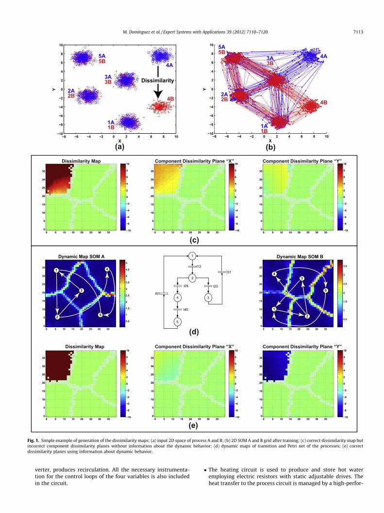
Fig. 1 shows a trivial example to illustrate the previous idea. Thetwo processes involved in this example, A and B, describe 5 clusters(1A,2A, . . . ,5A,1B, . . . ,5B) and only two input variables x and y areconsidered to facilitate the interpretation. Obviously, this ideashould be extrapolated to situations where the dimension is high-er. In the dissimilarity map we can see an area, corresponding toone of the conditions of process B (condition 4), where the behav-ior of the processes is different. Dissimilarity maps are useful forunderstanding the changes in an industrial process or the differ-ences between equivalent industrial processes where each pair ofthe compared neurons represents the same state.

The selection of the BMU using Eq. (5), i.e., the nearest neuronwith a certain distance function, helps to detect anomalies in a sta-tic analysis. However, this selection criterion can lead to erroneousresults in industrial processes that have an implicit dynamicbehavior in the temporal variation of its state. This is especiallytrue regarding the identification of the variables associated withthe fault. The problem arises when the nearest neuron of the refer-ence process is not consistent with the dynamics of the monitoredprocess. In these cases, the dissimilarity assigned to the neuron isnot representative of the deviation between models. This problemcan be seen in the toy example in Fig. 1. Let us assume that bothprocesses, A and B, have a dynamic behavior that describes 5 pro-cess conditions with the sequence 1–2–3–1–2–4–5, as labeled inFig. 1c. The component dissimilarity planes obtained without anyprior knowledge about this sequence show that there has beenan anomaly in the variable x in the condition 4, but the fault is in-deed associated to variable y. This undesired effect has happenedbecause neurons describing state 4B are mapped on neurons ofstate 1A, according to the standard BMU assignment procedure,since cluster 1A is closer than cluster 4A. Obviously, a proper com-parison would require to refer to state 4A. In order to solve thisproblem, it is necessary to incorporate prior information aboutthe dynamic behavior of the process in SOM models and use thisinformation for the selection of BMUs.

3.3. Description of the procedure

Many methods have been proposed in order to extend the SOMto dynamic analysis (Barreto, 2007; Principe, Wang, & Motter,1998). Some techniques are based on post-processing the tradi-tional algorithm. These methods work with temporal relationshipsbetween successive winning neurons for the process data and areusually described as methods based on trajectories (Fuertes et al.,2010; Tryba & Goser, 1991). In particular, the dynamic model oftransitions described in Fuertes et al. (2010) clusters the SOM mod-

el and uses the path that encodes the evolution of successive win-ning neurons to obtain the transition probability matrix betweenthose clusters. Then, neurons are labeled as belonging to a cluster,which represents a process condition, and the transitions amongclusters are computed.

To build the dynamic model of transitions, the transition prob-ability between a given pair of process conditions, i and j, iscomputed, using:

pij ¼nijPnt

k¼1nikð6Þ

where nij is the number of transitions from the process conditions ito j and nt is the total number of conditions determined from theSOM clustering. The resulting model can be interpreted as a Petrinet (Murata, 1989) or a Markov chain (Norris, 1997): the processconditions are the places (represented by a circle) whereas the tran-sitions describe the reachable conditions from a given one. Thesetransitions between clusters encode the process dynamics.

We propose to use this model of transitions to restrict the set ofcandidate neurons from which the dissimilarity function can becomputed in order to overcome the problem presented above.Now, the BMU would not be computed just as the closest one,but as the unit with the minimum distance among those that obeythe dynamic behavior defined by the transition model, i.e., the neu-rons in SOM-A that belong to the same process condition and theones directly accessible from it.

Fig. 1 presents the results of applying this method to the toyexample described above. The results of the basic computationwithout dynamic information (see Fig. 1c) do not provide the cor-rect dissimilarity planes. The reason is that cluster 4B is comparedto 1A. Although the neurons corresponding to the first cluster inprocess A are certainly the closest ones to the faulty condition, theydo not follow the dynamic behavior of the process. This behavior,modeled by the dynamic model of transitions, is shown inFig. 1d. First, a SOM model for process A and its dynamic modelof transitions are calculated. Then, the SOM model for process B(initially without information on the dynamics of transitions) iscalculated and clustered using the u-matrix (Ultsch, 1993). Finally,the clusters in the process B are labeled in order to comply with thedynamic model of transitions obtained for process A. The maps inFig. 1e are obtained by selecting the BMUs only among the acces-sible clusters according to the dynamic model, i.e., the neurons la-beled with the same cluster number, 4A, or the only one that isdirectly reachable, 5A. With this approach, the component dissim-ilarity planes identify correctly that the deviation has been pro-duced exclusively in the variable y of the process B. Therefore,the dynamic behavior implicit in the model of transitions helpsto solve the problem.

4. Monitoring architecture

The experiments designed to test dissimilarity maps for batchprocess monitoring use two real industrial process plants thatimplement the same process. These plants were developed bythe Institute for Automatic Control and Manufacturing at the Uni-versity of León, with research purposes (Domínguez, Fuertes, Reg-uera, González, & Ramón, 2004). They are located in their facilitiesand connected to the Remote Laboratory of Automatic Control(http://lra.unileon.es) of the University of León. Each plant is com-posed of a main circuit and two utility circuits:

� The process circuit is designed to control four physical vari-ables: pressure, flow, level and temperature. It contains twocascade tanks of 5 and 6.5 l each, which are associated to thelevel control loops. A centrifugal pump, driven by an AC con-

0 10

0

10

X

Y

Dissimilarity

−8 −6 −4 −2 0 2 4 6 8 10−10

−8

−6

−4

−2

0

2

4

6

8

10

X

Y

4B

1B

2B

3B

5B4A

1A

2A

3A

5A

Dynamic Map SOM A

0 5 10 15 20 25 30 350

5

10

15

20

25

30

35

0.5

1

1.5

2

2.5

3

3.5

4

4.5

5

3

5

4

2

1

1

2

34

t12

t24 t23

t31

t51

t45

5

Dynamic Map SOM B

0 5 10 15 20 25 30 350

5

10

15

20

25

30

35

0.5

1

1.5

2

2.5

3

3.5

3

1

2

4

5

(a) (b)

(c)

(d)

(e)

Component Dissimilarity Plane “X”

Component Dissimilarity Plane “X” Component Dissimilarity Plane “Y”

Component Dissimilarity Plane “Y”Dissimilarity Map

Dissimilarity Map

Fig. 1. Simple example of generation of the dissimilarity maps; (a) input 2D space of process A and B; (b) 2D SOM A and B grid after training; (c) correct dissimilarity map butincorrect component dissimilarity planes without information about the dynamic behavior; (d) dynamic maps of transition and Petri net of the processes; (e) correctdissimilarity planes using information about dynamic behavior.

M. Domínguez et al. / Expert Systems with Applications 39 (2012) 7110–7120 7113

verter, produces recirculation. All the necessary instrumenta-tion for the control loops of the four variables is also includedin the circuit.

� The heating circuit is used to produce and store hot wateremploying electric resistors with static adjustable drives. Theheat transfer to the process circuit is managed by a high-perfor-

7114 M. Domínguez et al. / Expert Systems with Applications 39 (2012) 7110–7120

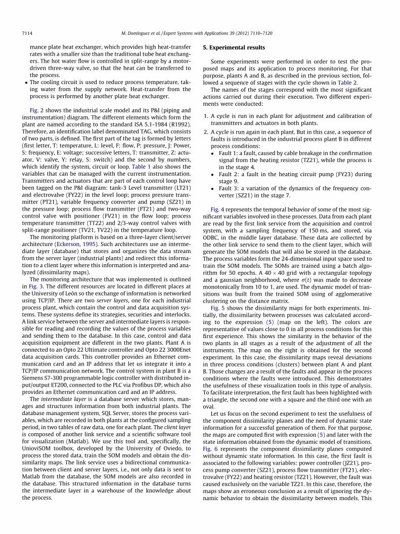
mance plate heat exchanger, which provides high heat-transferrates with a smaller size than the traditional tube heat exchang-ers. The hot water flow is controlled in split-range by a motor-driven three-way valve, so that the heat can be transferred tothe process.� The cooling circuit is used to reduce process temperature, tak-

ing water from the supply network. Heat-transfer from theprocess is performed by another plate heat exchanger.

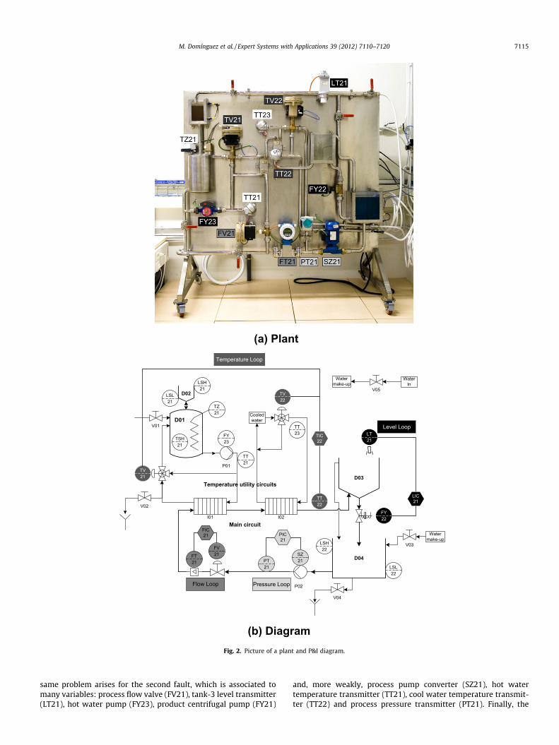
Fig. 2 shows the industrial scale model and its P&I (piping andinstrumentation) diagram. The different elements which form theplant are named according to the standard ISA 5.1-1984 (R1992).Therefore, an identification label denominated TAG, which consistsof two parts, is defined. The first part of the tag is formed by letters(first letter, T: temperature, L: level, F: flow, P: pressure, J: Power,S: frequency, E: voltage; successive letters, T: transmitter, Z: actu-ator, V: valve, Y: relay, S: switch) and the second by numbers,which identify the system, circuit or loop. Table 1 also shows thevariables that can be managed with the current instrumentation.Transmitters and actuators that are part of each control loop havebeen tagged on the P&I diagram: tank-3 Level transmitter (LT21)and electrovalve (FY22) in the level loop; process pressure trans-mitter (PT21), variable frequency converter and pump (SZ21) inthe pressure loop; process flow transmitter (FT21) and two-waycontrol valve with positioner (FV21) in the flow loop; processtemperature transmitter (TT22) and 2/3-way control valves withsplit-range positioner (TV21, TV22) in the temperature loop.

The monitoring platform is based on a three-layer client/serverarchitecture (Eckerson, 1995). Such architectures use an interme-diate layer (database) that stores and organizes the data streamfrom the server layer (industrial plants) and redirect this informa-tion to a client layer where this information is interpreted and ana-lyzed (dissimilarity maps).

The monitoring architecture that was implemented is outlinedin Fig. 3. The different resources are located in different places atthe University of León so the exchange of information is networkedusing TCP/IP. There are two server layers, one for each industrialprocess plant, which contain the control and data acquisition sys-tems. These systems define its strategies, securities and interlocks.A link service between the server and intermediate layers is respon-sible for reading and recording the values of the process variablesand sending them to the database. In this case, control and dataacquisition equipment are different in the two plants. Plant A isconnected to an Opto 22 Ultimate controller and Opto 22 3000Enetdata acquisition cards. This controller provides an Ethernet com-munication card and an IP address that let us integrate it into aTCP/IP communication network. The control system in plant B is aSiemens S7-300 programmable logic controller with distributed in-put/output ET200, connected to the PLC via Profibus DP, which alsoprovides an Ethernet communication card and an IP address.

The intermediate layer is a database server which stores, man-ages and structures information from both industrial plants. Thedatabase management system, SQL Server, stores the process vari-ables, which are recorded in both plants at the configured samplingperiod, in two tables of raw data, one for each plant. The client layeris composed of another link service and a scientific software toolfor visualization (Matlab). We use this tool and, specifically, theUnioviSOM toolbox, developed by the University of Oviedo, toprocess the stored data, train the SOM models and obtain the dis-similarity maps. The link service uses a bidirectional communica-tion between client and server layers, i.e., not only data is sent toMatlab from the database, the SOM models are also recorded inthe database. This structured information in the database turnsthe intermediate layer in a warehouse of the knowledge aboutthe process.

5. Experimental results

Some experiments were performed in order to test the pro-posed maps and its application to process monitoring. For thatpurpose, plants A and B, as described in the previous section, fol-lowed a sequence of stages with the cycle shown in Table 2.

The names of the stages correspond with the most significantactions carried out during their execution. Two different experi-ments were conducted:

1. A cycle is run in each plant for adjustment and calibration oftransmitters and actuators in both plants.

2. A cycle is run again in each plant. But in this case, a sequence offaults is introduced in the industrial process plant B in differentprocess conditions:� Fault 1: a fault, caused by cable breakage in the confirmation

signal from the heating resistor (TZ21), while the process isin the stage 4.

� Fault 2: a fault in the heating circuit pump (FY23) duringstage 9.

� Fault 3: a variation of the dynamics of the frequency con-verter (SZ21) in the stage 7.

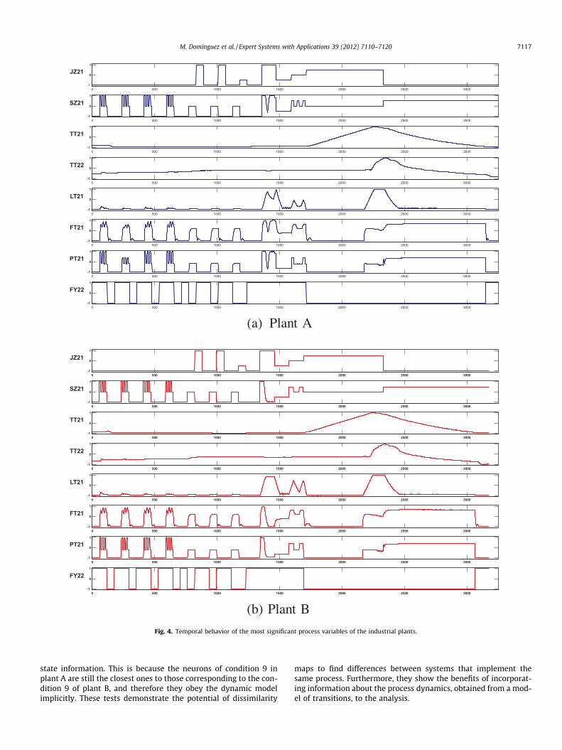
Fig. 4 represents the temporal behavior of some of the most sig-nificant variables involved in these processes. Data from each plantare read by the first link service from the acquisition and controlsystem, with a sampling frequency of 150 ms, and stored, viaODBC, in the middle layer database. These data are collected bythe other link service to send them to the client layer, which willgenerate the SOM models that will also be stored in the database.The process variables form the 24-dimensional input space used totrain the SOM models. The SOMs are trained using a batch algo-rithm for 50 epochs. A 40 � 40 grid with a rectangular topologyand a gaussian neighborhood, where r(t) was made to decreasemonotonically from 10 to 1, are used. The dynamic model of tran-sitions was built from the trained SOM using of agglomerativeclustering on the distance matrix.

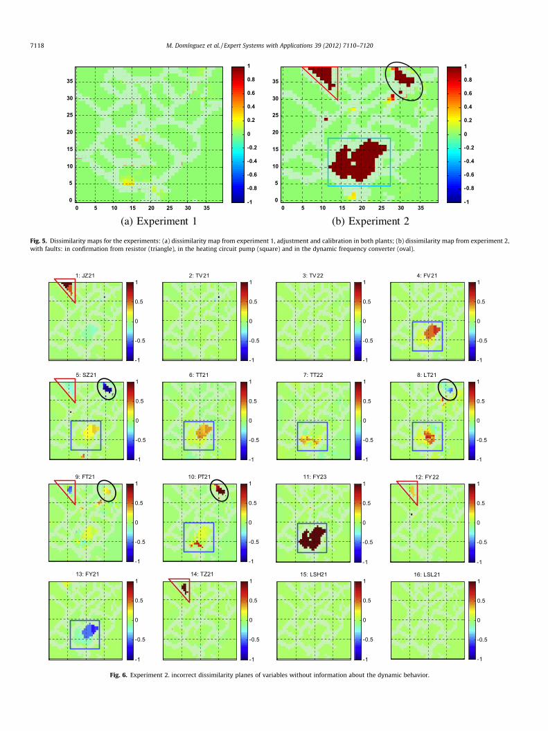
Fig. 5 shows the dissimilarity maps for both experiments. Ini-tially, the dissimilarity between processes was calculated accord-ing to the expression (5) (map on the left). The colors arerepresentative of values close to 0 in all process conditions for thisfirst experience. This shows the similarity in the behavior of thetwo plants in all stages as a result of the adjustment of all theinstruments. The map on the right is obtained for the secondexperiment. In this case, the dissimilarity maps reveal deviationsin three process conditions (clusters) between plant A and plantB. Those changes are a result of the faults and appear in the processconditions where the faults were introduced. This demonstratesthe usefulness of these visualization tools in this type of analysis.To facilitate interpretation, the first fault has been highlighted witha triangle, the second one with a square and the third one with anoval.

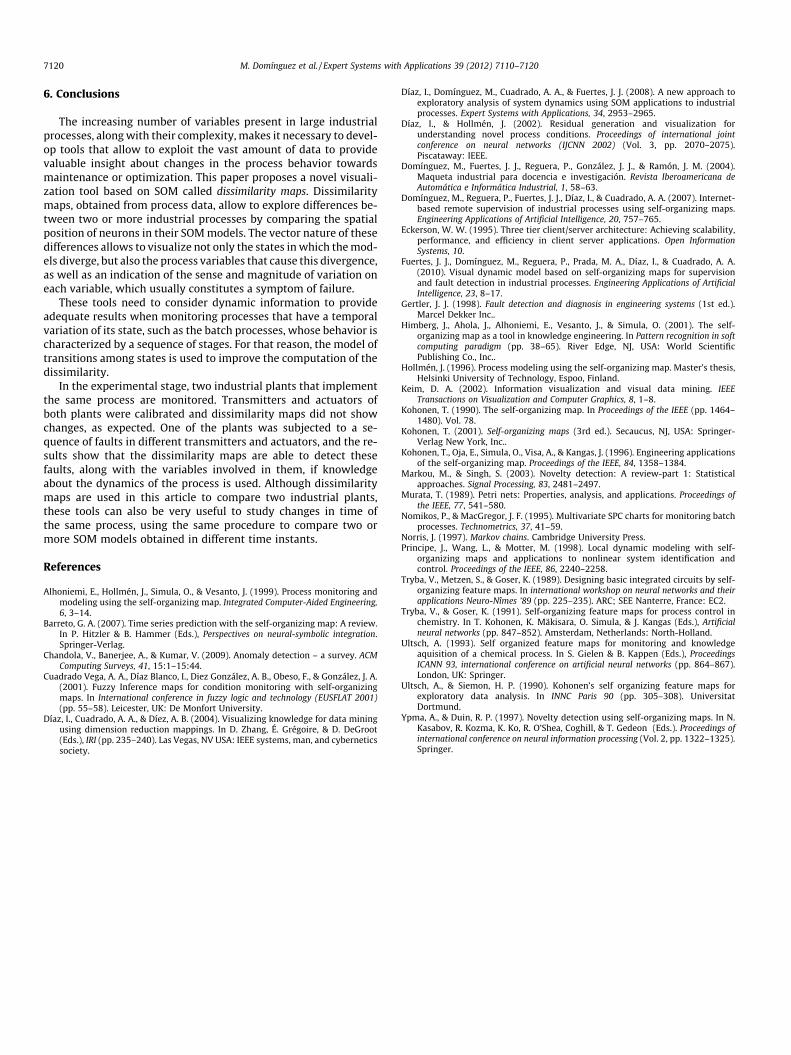
Let us focus on the second experiment to test the usefulness ofthe component dissimilarity planes and the need of dynamic stateinformation for a successful generation of them. For that purpose,the maps are computed first with expression (5) and later with thestate information obtained from the dynamic model of transitions.Fig. 6 represents the component dissimilarity planes computedwithout dynamic state information. In this case, the first fault isassociated to the following variables: power controller (JZ21), pro-cess pump converter (SZ21), process flow transmitter (FT21), elec-trovalve (FY22) and heating resistor (TZ21). However, the fault wascaused exclusively on the variable TZ21. In this case, therefore, themaps show an erroneous conclusion as a result of ignoring the dy-namic behavior to obtain the dissimilarity between models. This

(a) Plant

D01

D02

LSH21

LSL21

V01

TZ21

P01

I01 I02

TV21

TT22

TT21

Cooledwater

D03

D04

P02

PT21

FV21FT

21

SZ21

LSH22

TSH21

V02

V04

Watermake-up

V03

Temperature utility circuits

Main circuit

TV22

LSL22

TT23

FY22

FY23

TIC22

PIC21

FIC21

LIC21

WaterIn

Watermake-up

V05

LT21

Level Loop

Temperature Loop

Pressure LoopFlow Loop

(b) DiagramFig. 2. Picture of a plant and P&I diagram.

M. Domínguez et al. / Expert Systems with Applications 39 (2012) 7110–7120 7115

same problem arises for the second fault, which is associated tomany variables: process flow valve (FV21), tank-3 level transmitter(LT21), hot water pump (FY23), product centrifugal pump (FY21)

and, more weakly, process pump converter (SZ21), hot watertemperature transmitter (TT21), cool water temperature transmit-ter (TT22) and process pressure transmitter (PT21). Finally, the

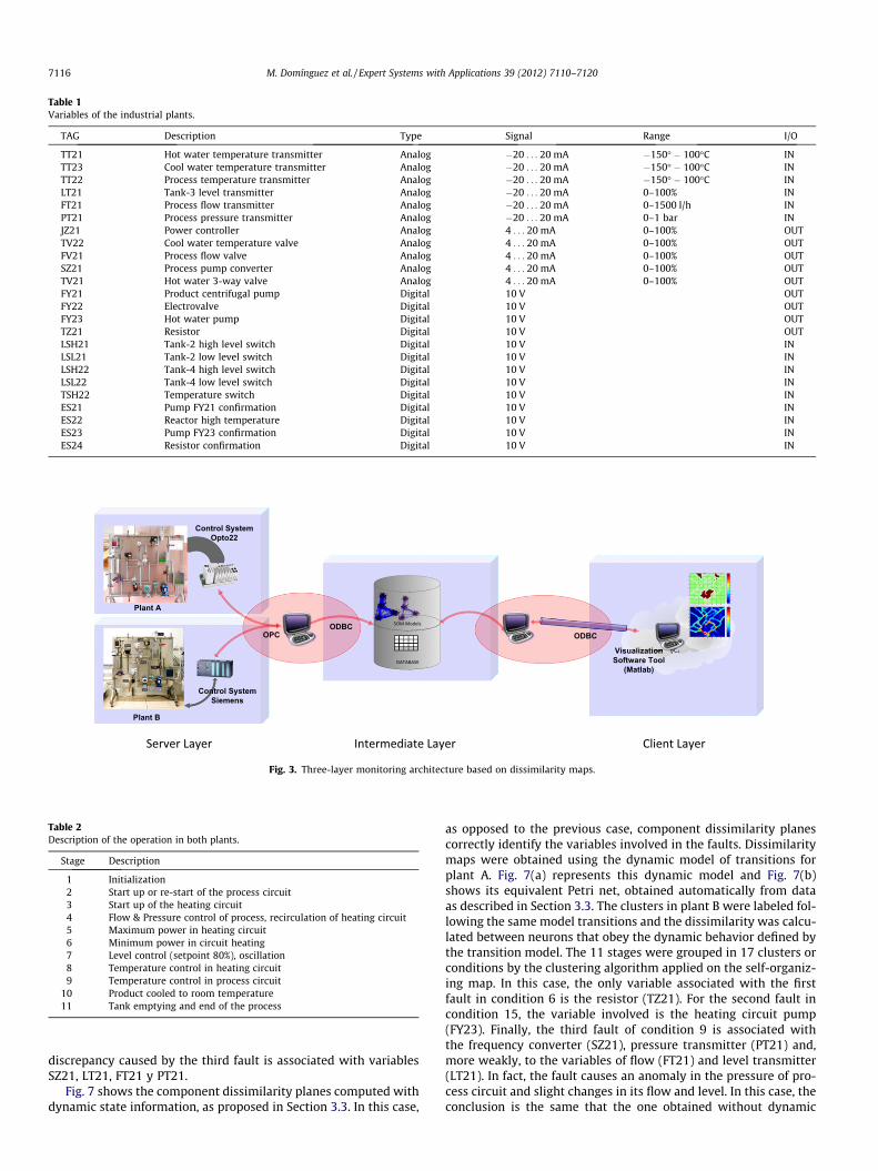
Table 1Variables of the industrial plants.

TAG Description Type Signal Range I/O

TT21 Hot water temperature transmitter Analog �20 . . . 20 mA �150� � 100�C INTT23 Cool water temperature transmitter Analog �20 . . . 20 mA �150� � 100�C INTT22 Process temperature transmitter Analog �20 . . . 20 mA �150� � 100�C INLT21 Tank-3 level transmitter Analog �20 . . . 20 mA 0–100% INFT21 Process flow transmitter Analog �20 . . . 20 mA 0–1500 l/h INPT21 Process pressure transmitter Analog �20 . . . 20 mA 0–1 bar INJZ21 Power controller Analog 4 . . . 20 mA 0–100% OUTTV22 Cool water temperature valve Analog 4 . . . 20 mA 0–100% OUTFV21 Process flow valve Analog 4 . . . 20 mA 0–100% OUTSZ21 Process pump converter Analog 4 . . . 20 mA 0–100% OUTTV21 Hot water 3-way valve Analog 4 . . . 20 mA 0–100% OUTFY21 Product centrifugal pump Digital 10 V OUTFY22 Electrovalve Digital 10 V OUTFY23 Hot water pump Digital 10 V OUTTZ21 Resistor Digital 10 V OUTLSH21 Tank-2 high level switch Digital 10 V INLSL21 Tank-2 low level switch Digital 10 V INLSH22 Tank-4 high level switch Digital 10 V INLSL22 Tank-4 low level switch Digital 10 V INTSH22 Temperature switch Digital 10 V INES21 Pump FY21 confirmation Digital 10 V INES22 Reactor high temperature Digital 10 V INES23 Pump FY23 confirmation Digital 10 V INES24 Resistor confirmation Digital 10 V IN

Fig. 3. Three-layer monitoring architecture based on dissimilarity maps.

Table 2Description of the operation in both plants.

Stage Description

1 Initialization2 Start up or re-start of the process circuit3 Start up of the heating circuit4 Flow & Pressure control of process, recirculation of heating circuit5 Maximum power in heating circuit6 Minimum power in circuit heating7 Level control (setpoint 80%), oscillation8 Temperature control in heating circuit9 Temperature control in process circuit

10 Product cooled to room temperature11 Tank emptying and end of the process

7116 M. Domínguez et al. / Expert Systems with Applications 39 (2012) 7110–7120

discrepancy caused by the third fault is associated with variablesSZ21, LT21, FT21 y PT21.

Fig. 7 shows the component dissimilarity planes computed withdynamic state information, as proposed in Section 3.3. In this case,

as opposed to the previous case, component dissimilarity planescorrectly identify the variables involved in the faults. Dissimilaritymaps were obtained using the dynamic model of transitions forplant A. Fig. 7(a) represents this dynamic model and Fig. 7(b)shows its equivalent Petri net, obtained automatically from dataas described in Section 3.3. The clusters in plant B were labeled fol-lowing the same model transitions and the dissimilarity was calcu-lated between neurons that obey the dynamic behavior defined bythe transition model. The 11 stages were grouped in 17 clusters orconditions by the clustering algorithm applied on the self-organiz-ing map. In this case, the only variable associated with the firstfault in condition 6 is the resistor (TZ21). For the second fault incondition 15, the variable involved is the heating circuit pump(FY23). Finally, the third fault of condition 9 is associated withthe frequency converter (SZ21), pressure transmitter (PT21) and,more weakly, to the variables of flow (FT21) and level transmitter(LT21). In fact, the fault causes an anomaly in the pressure of pro-cess circuit and slight changes in its flow and level. In this case, theconclusion is the same that the one obtained without dynamic

0 500 1000 1500 2000 2500 3000-1

0

1

JZ21

0 500 1000 1500 2000 2500 3000-1

0

1

SZ21

0 500 1000 1500 2000 2500 3000-1

0

1

TT21

0 500 1000 1500 2000 2500 3000-1

0

1

TT22

0 500 1000 1500 2000 2500 3000-1

0

1

LT21

0 500 1000 1500 2000 2500 3000-1

0

1

FT21

0 500 1000 1500 2000 2500 3000-1

0

1

PT21

0 500 1000 1500 2000 2500 3000-1

0

1

FY22

(a) Plant A

0 500 1000 1500 2000 2500 3000-1

0

1

JZ21

0 500 1000 1500 2000 2500 3000-1

0

1

SZ21

0 500 1000 1500 2000 2500 3000-1

0

1

TT21

0 500 1000 1500 2000 2500 3000-1

0

1

TT22

0 500 1000 1500 2000 2500 3000-1

0

1

LT21

0 500 1000 1500 2000 2500 3000-1

0

1

FT21

0 500 1000 1500 2000 2500 3000-1

0

1

PT21

0 500 1000 1500 2000 2500 3000-1

0

1

FY22

(b) Plant B

Fig. 4. Temporal behavior of the most significant process variables of the industrial plants.

M. Domínguez et al. / Expert Systems with Applications 39 (2012) 7110–7120 7117

state information. This is because the neurons of condition 9 inplant A are still the closest ones to those corresponding to the con-dition 9 of plant B, and therefore they obey the dynamic modelimplicitly. These tests demonstrate the potential of dissimilarity

maps to find differences between systems that implement thesame process. Furthermore, they show the benefits of incorporat-ing information about the process dynamics, obtained from a mod-el of transitions, to the analysis.

0 5 10 15 20 25 30 350

5

10

15

20

25

30

35

-1

-0.8

-0.6

-0.4

-0.2

0

0.2

0.4

0.6

0.8

1

(a) Experiment 10 5 10 15 20 25 30 35

0

5

10

15

20

25

30

35

-1

-0.8

-0.6

-0.4

-0.2

0

0.2

0.4

0.6

0.8

1

(b) Experiment 2

Fig. 5. Dissimilarity maps for the experiments: (a) dissimilarity map from experiment 1, adjustment and calibration in both plants; (b) dissimilarity map from experiment 2,with faults: in confirmation from resistor (triangle), in the heating circuit pump (square) and in the dynamic frequency converter (oval).

9: FT21

-1

-0.5

0

0.5

110: PT21

-1

-0.5

0

0.5

1

-1

-0.5

0

0.5

112: FY22

-1

-0.5

0

0.5

1

-1

-0.5

0

0.5

1

-1

-0.5

0

0.5

115: LSH21

-1

-0.5

0

0.5

116: LSL21

-1

-0.5

0

0.5

1

1: JZ21

-1

-0.5

0

0.5

12: TV21

-1

-0.5

0

0.5

13: TV22

-1

-0.5

0

0.5

14: FV21

-1

-0.5

0

0.5

1

5: SZ21

-1

-0.5

0

0.5

16: TT21

-1

-0.5

0

0.5

17: TT22

-1

-0.5

0

0.5

18: LT21

-1

-0.5

0

0.5

1

11: FY23

13: FY21 14: TZ21

Fig. 6. Experiment 2. incorrect dissimilarity planes of variables without information about the dynamic behavior.

7118 M. Domínguez et al. / Expert Systems with Applications 39 (2012) 7110–7120

0 5 10 15 20 25 30 350

5

10

15

20

25

30

35

0.5

1

1.5

2

2.5

17

16

15

6

14

5

3218

7

4

1

10

11

9

13

12

8

(a) Process A

p1

p5p2

p6p3 p7

p4

p8 p9 p10

p11p12

p13 p14

p15p16p17

(b) Petri net0 5 10 15 20 25 30 35

0

5

10

15

20

25

30

35

0.5

1

1.5

2

2.5

17

16

15

6

14

5

3

218

7

4

1

10

11

9

13

12

88

10

15

6

1

(c) Process B

1: JZ21

-1

-0.5

0

0.5

12: TV21

-1

-0.5

0

0.5

13: TV22

-1

-0.5

0

0.5

14: FV21

-1

-0.5

0

0.5

1

16: LSL21

-1

-0.5

0

0.5

113: P02

-1

-0.5

0

0.5

114: R1

-1

-0.5

0

0.5

115: LSH21

-1

-0.5

0

0.5

1

9: FT21

-1

-0.5

0

0.5

110: PT21

-1

-0.5

0

0.5

111: P01

-1

-0.5

0

0.5

112: FY22

-1

-0.5

0

0.5

1

6: TT21

-1

-0.5

0

0.5

17: TT22

-1

-0.5

0

0.5

18: LT21

-1

-0.5

0

0.5

15: SZ21

-1

-0.5

0

0.5

1

11: FY23

14: TZ2113: FY21

(d) Component dissimilarity planes

Fig. 7. Experiment 2. correct dissimilarity planes of variables with information about the dynamic behavior: (a) dynamic map of transitions of process A; (b) petri net ofprocess A obtained from data; (c) dynamic map of transitions of process B labeled in agreement with process A; (d) dissimilarity planes obtained using information aboutdynamic behavior.

M. Domínguez et al. / Expert Systems with Applications 39 (2012) 7110–7120 7119

7120 M. Domínguez et al. / Expert Systems with Applications 39 (2012) 7110–7120

6. Conclusions

The increasing number of variables present in large industrialprocesses, along with their complexity, makes it necessary to devel-op tools that allow to exploit the vast amount of data to providevaluable insight about changes in the process behavior towardsmaintenance or optimization. This paper proposes a novel visuali-zation tool based on SOM called dissimilarity maps. Dissimilaritymaps, obtained from process data, allow to explore differences be-tween two or more industrial processes by comparing the spatialposition of neurons in their SOM models. The vector nature of thesedifferences allows to visualize not only the states in which the mod-els diverge, but also the process variables that cause this divergence,as well as an indication of the sense and magnitude of variation oneach variable, which usually constitutes a symptom of failure.

These tools need to consider dynamic information to provideadequate results when monitoring processes that have a temporalvariation of its state, such as the batch processes, whose behavior ischaracterized by a sequence of stages. For that reason, the model oftransitions among states is used to improve the computation of thedissimilarity.

In the experimental stage, two industrial plants that implementthe same process are monitored. Transmitters and actuators ofboth plants were calibrated and dissimilarity maps did not showchanges, as expected. One of the plants was subjected to a se-quence of faults in different transmitters and actuators, and the re-sults show that the dissimilarity maps are able to detect thesefaults, along with the variables involved in them, if knowledgeabout the dynamics of the process is used. Although dissimilaritymaps are used in this article to compare two industrial plants,these tools can also be very useful to study changes in time ofthe same process, using the same procedure to compare two ormore SOM models obtained in different time instants.

References

Alhoniemi, E., Hollmén, J., Simula, O., & Vesanto, J. (1999). Process monitoring andmodeling using the self-organizing map. Integrated Computer-Aided Engineering,6, 3–14.

Barreto, G. A. (2007). Time series prediction with the self-organizing map: A review.In P. Hitzler & B. Hammer (Eds.), Perspectives on neural-symbolic integration.Springer-Verlag.

Chandola, V., Banerjee, A., & Kumar, V. (2009). Anomaly detection – a survey. ACMComputing Surveys, 41, 15:1–15:44.

Cuadrado Vega, A. A., Díaz Blanco, I., Diez González, A. B., Obeso, F., & González, J. A.(2001). Fuzzy Inference maps for condition monitoring with self-organizingmaps. In International conference in fuzzy logic and technology (EUSFLAT 2001)(pp. 55–58). Leicester, UK: De Monfort University.

Díaz, I., Cuadrado, A. A., & Díez, A. B. (2004). Visualizing knowledge for data miningusing dimension reduction mappings. In D. Zhang, É. Grégoire, & D. DeGroot(Eds.), IRI (pp. 235–240). Las Vegas, NV USA: IEEE systems, man, and cyberneticssociety.

Díaz, I., Domínguez, M., Cuadrado, A. A., & Fuertes, J. J. (2008). A new approach toexploratory analysis of system dynamics using SOM applications to industrialprocesses. Expert Systems with Applications, 34, 2953–2965.

Díaz, I., & Hollmén, J. (2002). Residual generation and visualization forunderstanding novel process conditions. Proceedings of international jointconference on neural networks (IJCNN 2002) (Vol. 3, pp. 2070–2075).Piscataway: IEEE.

Domínguez, M., Fuertes, J. J., Reguera, P., González, J. J., & Ramón, J. M. (2004).Maqueta industrial para docencia e investigación. Revista Iberoamericana deAutomática e Informática Industrial, 1, 58–63.

Domínguez, M., Reguera, P., Fuertes, J. J., Díaz, I., & Cuadrado, A. A. (2007). Internet-based remote supervision of industrial processes using self-organizing maps.Engineering Applications of Artificial Intelligence, 20, 757–765.

Eckerson, W. W. (1995). Three tier client/server architecture: Achieving scalability,performance, and efficiency in client server applications. Open InformationSystems, 10.

Fuertes, J. J., Domínguez, M., Reguera, P., Prada, M. A., Díaz, I., & Cuadrado, A. A.(2010). Visual dynamic model based on self-organizing maps for supervisionand fault detection in industrial processes. Engineering Applications of ArtificialIntelligence, 23, 8–17.

Gertler, J. J. (1998). Fault detection and diagnosis in engineering systems (1st ed.).Marcel Dekker Inc..

Himberg, J., Ahola, J., Alhoniemi, E., Vesanto, J., & Simula, O. (2001). The self-organizing map as a tool in knowledge engineering. In Pattern recognition in softcomputing paradigm (pp. 38–65). River Edge, NJ, USA: World ScientificPublishing Co., Inc..

Hollmén, J. (1996). Process modeling using the self-organizing map. Master’s thesis,Helsinki University of Technology, Espoo, Finland.

Keim, D. A. (2002). Information visualization and visual data mining. IEEETransactions on Visualization and Computer Graphics, 8, 1–8.

Kohonen, T. (1990). The self-organizing map. In Proceedings of the IEEE (pp. 1464–1480). Vol. 78.

Kohonen, T. (2001). Self-organizing maps (3rd ed.). Secaucus, NJ, USA: Springer-Verlag New York, Inc..

Kohonen, T., Oja, E., Simula, O., Visa, A., & Kangas, J. (1996). Engineering applicationsof the self-organizing map. Proceedings of the IEEE, 84, 1358–1384.

Markou, M., & Singh, S. (2003). Novelty detection: A review-part 1: Statisticalapproaches. Signal Processing, 83, 2481–2497.

Murata, T. (1989). Petri nets: Properties, analysis, and applications. Proceedings ofthe IEEE, 77, 541–580.

Nomikos, P., & MacGregor, J. F. (1995). Multivariate SPC charts for monitoring batchprocesses. Technometrics, 37, 41–59.

Norris, J. (1997). Markov chains. Cambridge University Press.Principe, J., Wang, L., & Motter, M. (1998). Local dynamic modeling with self-

organizing maps and applications to nonlinear system identification andcontrol. Proceedings of the IEEE, 86, 2240–2258.

Tryba, V., Metzen, S., & Goser, K. (1989). Designing basic integrated circuits by self-organizing feature maps. In international workshop on neural networks and theirapplications Neuro-Nîmes ’89 (pp. 225–235). ARC; SEE Nanterre, France: EC2.

Tryba, V., & Goser, K. (1991). Self-organizing feature maps for process control inchemistry. In T. Kohonen, K. Mäkisara, O. Simula, & J. Kangas (Eds.), Artificialneural networks (pp. 847–852). Amsterdam, Netherlands: North-Holland.

Ultsch, A. (1993). Self organized feature maps for monitoring and knowledgeaquisition of a chemical process. In S. Gielen & B. Kappen (Eds.), ProceedingsICANN 93, international conference on artificial neural networks (pp. 864–867).London, UK: Springer.

Ultsch, A., & Siemon, H. P. (1990). Kohonen’s self organizing feature maps forexploratory data analysis. In INNC Paris 90 (pp. 305–308). UniversitatDortmund.

Ypma, A., & Duin, R. P. (1997). Novelty detection using self-organizing maps. In N.Kasabov, R. Kozma, K. Ko, R. O’Shea, Coghill, & T. Gedeon (Eds.). Proceedings ofinternational conference on neural information processing (Vol. 2, pp. 1322–1325).Springer.