Self-Organizing Maps (SOMs) - Bioinformatics Graz · 2 4 Self-Organizing Map (SOM) • The...
22
1 2 Self-Organizing Maps (SOMs) • Resources – Mehotra, K., Mohan, C. K., & Ranka, S. (1997). Elements of Artificial Neural Networks. MIT Press • pp. 187-202 – Fausett, L. (1994). Fundamentals of Neural Networks. Prentice Hall. pp. 169-187 – Bibliography of SOM papers • http://citeseer.ist.psu.edu/104693.html • http://www.cis.hut.fi/research/som-bibl/ – Java applet & tutorial information • http://davis.wpi.edu/~matt/courses/soms/ – WEBSOM - Self-Organizing Maps for Internet Exploration • http://websom.hut.fi/websom/ 3 Supervised vs. Unsupervised Learning • An important aspect of an ANN model is whether it needs guidance in learning or not. Based on the way they learn, all artificial neural networks can be divided into two learning categories - supervised and unsupervised. • In supervised learning, a desired output result for each input vector is required when the network is trained. An ANN of the supervised learning type, such as the multi-layer perceptron, uses the target result to guide the formation of the neural parameters. It is thus possible to make the neural network learn the behavior of the process under study. • In unsupervised learning, the training of the network is entirely data-driven and no target results for the input data vectors are provided. An ANN of the unsupervised learning type, such as the self-organizing map, can be used for clustering the input data and find features inherent to the problem.
Transcript of Self-Organizing Maps (SOMs) - Bioinformatics Graz · 2 4 Self-Organizing Map (SOM) • The...

1
2
Self-Organizing Maps (SOMs)
• Resources– Mehotra, K., Mohan, C. K., & Ranka, S. (1997). Elements
of Artificial Neural Networks. MIT Press• pp. 187-202
– Fausett, L. (1994). Fundamentals of Neural Networks. Prentice Hall. pp. 169-187
– Bibliography of SOM papers• http://citeseer.ist.psu.edu/104693.html• http://www.cis.hut.fi/research/som-bibl/
– Java applet & tutorial information• http://davis.wpi.edu/~matt/courses/soms/
– WEBSOM - Self-Organizing Maps for Internet Exploration• http://websom.hut.fi/websom/
3
Supervised vs. Unsupervised Learning
• An important aspect of an ANN model is whether it needs guidance in learning or not. Based on the way they learn, all artificial neural networks can be divided into two learning categories - supervised and unsupervised.
• In supervised learning, a desired output result for each input vector is required when the network is trained. An ANN of the supervised learning type, such as the multi-layer perceptron, uses the target result to guide the formation of the neural parameters. It is thus possible to make the neural network learn the behavior of the process under study.
• In unsupervised learning, the training of the network is entirely data-driven and no target results for the input data vectors are provided. An ANN of the unsupervised learning type, such as the self-organizing map, can be used for clustering the input data and find features inherent to the problem.

2
4
Self-Organizing Map (SOM)
• The Self-Organizing Map was developed by professor Kohonen. The SOM has been proven useful in many applications
• One of the most popular neural network models. It belongs to the category of competitive learning networks.
• Based on unsupervised learning, which means that no human intervention is needed during the learning and that little needsto be known about the characteristics of the input data.
• Use the SOM for clustering data without knowing the class memberships of the input data. The SOM can be used to detect features inherent to the problem and thus has also been called SOFM, the Self-Organizing Feature Map.
5
Self-Organizing Map (cont.)
• Provides a topology preserving mapping from the high dimensional space to map units. Map units, or neurons, usually form a two-dimensional lattice and thus the mapping is a mapping from high dimensional space onto a plane.
• The property of topology preserving means that the mapping preserves the relative distance between the points. Points that are near each other in the input space are mapped to nearby map units in the SOM. The SOM can thus serve as a cluster analyzing tool of high-dimensional data. Also, the SOM has the capability to generalize
• Generalization capability means that the network can recognize or characterize inputs it has never encountered before. A new input is assimilated with the map unit it is mapped to.

3
6
The general problem
• How can an algorithm learn without supervision?– I.e., without a “teacher”
7
Self-Organizing Maps (SOM’s)
• Categorization method• A neural network technique• Unsupervised

4
8
Input & Output• Training data: vectors, X
– Vectors of length n(x1,1, x1,2, ..., x1,i,…, x1,n)(x2,1, x2,2, ..., x2,i,…, x2,n)…(xj,1, xj,2, ..., xj,i,…, xj,n)…(xp,1, xp,2, ..., xp,i,…, xp,n)
– Vector components are real numbers• Outputs
– A vector, Y, of length m: (y1, y2, ..., yi,…, ym)• Sometimes m < n, sometimes m > n, sometimes m = n
– Each of the p vectors in the training data is classified as falling in one of m clusters or categories
– That is: Which category does the training vector fall into?• Generalization
– For a new vector: (xj,1, xj,2, ..., xj,i,…, xj,n) – Which of the m categories (clusters) does it fall into?
p distinct training vectors
9
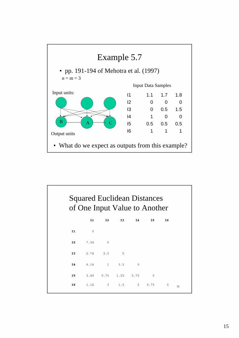
Network Architecture
• Two layers of units– Input: n units (length of training vectors)– Output: m units (number of categories)
• Input units fully connected with weights to output units
• Intra-layer (“lateral”) connections– Within output layer– Defined according to some topology– No weight between these connections, but used in
algorithm for updating weights
5
10
Network Architecture
X1 Xi Xn
Y1 Yi Ym
Inputs:
Outputs:
Note: There is one weight vector of length nassociated with each output unit
… …
… …m output units
n input units
11
Overall SOM Algorithm• Training
– Select output layer topology– Train weights connecting inputs to outputs– Topology is used, in conjunction with current mapping
of inputs to outputs, to define which weights will be updated
– Distance measure using the topology is reduced over time; reduces the number of weights that get updated per iteration
– Learning rate is reduced over time• Testing
– Use weights from training

6
12
Output Layer Topology• Often view output in spatial manner
– E.g., a 1D or 2D arrangement• 1D arrangement
– Topology defines which output layer units are neighbors with which others
– Have a function, D(t), which gives output unit neighborhood as a function of time (iterations) of the training algorithm
• E.g., 3 output units
B A C
D(t) = 1 means update weight B & A if input maps onto B
13
Example: 2D Output Layer Topology
R G B
Fully-connected weights
…50 units
… 50 units
* Function, D(t), can give output unit radius as a function of time (iterations) when training the weights* Usually, initially wide radius, changing to gradually narrower

7
14
Self Organizing Maps
• Often SOM’s are used with 2D topographies connecting the output units
• In this way, the final output can be interpreted spatially, i.e., as a map
15
SOM Algorithm• Select output layer network topology
– Initialize current neighborhood distance, D(0), to a positive value• Initialize weights from inputs to outputs to small random values• Let t = 1• While computational bounds are not exceeded do
1) Select an input sample2) Compute the square of the Euclidean distance offrom weight vectors (wj) associated with each output node
3) Select output node j* that has weight vector with minimum value from step 2)
4) Update weights to all nodes within a topological distance given by D(t) from j*, using the weight update rule:
5) Increment t• Endwhile
From Mehotra et al. (1997), p. 189
2
1 ,, ))((∑ =−
n
k kjkl twi
lili
))()(()()1( twittwtw jljj −+=+ η
1)1()(0 ≤−≤< tt ηηLearning rate generally decreases with time:

8
16
Example Self-Organizing Map
• From Fausett (1994)• n = 4, m = 2
• Training samplesi1: (1, 1, 0, 0)i2: (0, 0, 0, 1)i3: (1, 0, 0, 0)i4: (0, 0, 1, 1)
Input units:
Output units: 1 2
What should we expect as outputs?
Network Architecture
17
What are the Euclidean Distances Between the Data Samples?
• Training samplesi1: (1, 1, 0, 0)i2: (0, 0, 0, 1)i3: (1, 0, 0, 0)i4: (0, 0, 1, 1)
0i40i3
0i20i1
i4i3i2i1

9
Euclidean Distances Between Data Samples
• Training samplesi1: (1, 1, 0, 0)i2: (0, 0, 0, 1)i3: (1, 0, 0, 0)i4: (0, 0, 1, 1)
0314i4021i3
03i20i1
i4i3i2i1
Input units:
Output units: 1 2 What might we expect from the SOM?
19
Example Details• Training samples
i1: (1, 1, 0, 0)i2: (0, 0, 0, 1)i3: (1, 0, 0, 0)i4: (0, 0, 1, 1)
• Let neighborhood = 0– Only update weights associated with winning output unit (cluster) at each
iteration• Learning rate
η(t) = 0.6; 1 <= t <= 4η(t) = 0.5 η(1); 5 <= t <= 8η(t) = 0.5 η(5); 9 <= t <= 12etc.
• Initial weight matrix(random values between 0 and 1)
Input units:
Output units: 1 2
⎥⎦
⎤⎢⎣
⎡3.7.4.8.9.5.6.2.
2
1 ,, ))((∑ =−
n
k kjkl twi
))()(()()1( twittwtw jljj −+=+ η
d2 = (Euclidean distance)2 =
Weight update:
Unit 1:
Unit 2:
Problem: Calculate the weight updates for the first four steps

10
20
First Weight Update
• Training sample: i1– Unit 1 weights
• d2 = (.2-1)2 + (.6-1)2 + (.5-0)2 + (.9-0)2 = 1.86– Unit 2 weights
• d2 = (.8-1)2 + (.4-1)2 + (.7-0)2 + (.3-0)2 = .98– Unit 2 wins– Weights on winning unit are updated
– Giving an updated weight matrix:
⎥⎦
⎤⎢⎣
⎡3.7.4.8.9.5.6.2.Unit 1:
Unit 2:
i1: (1, 1, 0, 0)i2: (0, 0, 0, 1)i3: (1, 0, 0, 0)i4: (0, 0, 1, 1)
])3.7.4.8.[-0] 0 1 [1(6.0]3.7.4.8.[2 =+=−− weightsunitnew
= [.92 .76 .28 .12]
⎥⎦
⎤⎢⎣
⎡12.9.
28.5.
76.6.
92.2.Unit 1:
Unit 2:
21
Second Weight Update
• Training sample: i2– Unit 1 weights
• d2 = (.2-0)2 + (.6-0)2 + (.5-0)2 + (.9-1)2 = .66– Unit 2 weights
• d2 = (.92-0)2 + (.76-0)2 + (.28-0)2 + (.12-1)2 = 2.28– Unit 1 wins– Weights on winning unit are updated
– Giving an updated weight matrix:
Unit 1:
Unit 2:
i1: (1, 1, 0, 0)i2: (0, 0, 0, 1)i3: (1, 0, 0, 0)i4: (0, 0, 1, 1)
])9.5.6.2.[-1] 0 0 [0(6.0]9.5.6.2.[1 =+=−− weightsunitnew
= [.08 .24 .20 .96]
Unit 1:
Unit 2:
⎥⎦
⎤⎢⎣
⎡12.9.
28.5.
76.6.
92.2.
⎥⎦
⎤⎢⎣
⎡12.96.
28.20.
76.24.
92.08.

11
22
Third Weight Update
• Training sample: i3– Unit 1 weights
• d2 = (.08-1)2 + (.24-0)2 + (.2-0)2 + (.96-0)2 = 1.87– Unit 2 weights
• d2 = (.92-1)2 + (.76-0)2 + (.28-0)2 + (.12-0)2 = 0.68– Unit 2 wins– Weights on winning unit are updated
– Giving an updated weight matrix:
Unit 1:
Unit 2:
i1: (1, 1, 0, 0)i2: (0, 0, 0, 1)i3: (1, 0, 0, 0)i4: (0, 0, 1, 1)
])12.28.76.92.[-0] 0 0 [1(6.0]12.28.76.92.[2 =+=−− weightsunitnew
= [.97 .30 .11 .05]
Unit 1:
Unit 2:
⎥⎦
⎤⎢⎣
⎡12.96.
28.20.
76.24.
92.08.
⎥⎦
⎤⎢⎣
⎡05.96.
11.20.
30.24.
97.08.
23
Fourth Weight Update
• Training sample: i4– Unit 1 weights
• d2 = (.08-0)2 + (.24-0)2 + (.2-1)2 + (.96-1)2 = .71– Unit 2 weights
• d2 = (.97-0)2 + (.30-0)2 + (.11-1)2 + (.05-1)2 = 2.74– Unit 1 wins– Weights on winning unit are updated
– Giving an updated weight matrix:
Unit 1:
Unit 2:
i1: (1, 1, 0, 0)i2: (0, 0, 0, 1)i3: (1, 0, 0, 0)i4: (0, 0, 1, 1)
])96.20.24.08.[-1] 1 0 [0(6.0]96.20.24.08.[1 =+=−− weightsunitnew
= [.03 .10 .68 .98]
Unit 1:
Unit 2: ⎥⎦
⎤⎢⎣
⎡05.98.
11.68.
30.10.
97.03.
⎥⎦
⎤⎢⎣
⎡05.96.
11.20.
30.24.
97.08.

12
24
Applying the SOM Algorithm
0.60Unit 14
0.60Unit 23
0.60Unit 12
0.60Unit 21
η(t)D(t)4321time (t)
Data sample utilized
‘winning’ output unit
Unit 1:
Unit 2: ⎥⎦
⎤⎢⎣
⎡00.1
05.
5.0
0.10
After many iterations (epochs) through the data set:
Did we get the clustering that we expected?
25
What clusters do thedata samples fall into?
Unit 1:
Unit 2: ⎥⎦
⎤⎢⎣
⎡00.1
05.
5.0
0.10
WeightsInput units:
Output units: 1 2
Training samplesi1: (1, 1, 0, 0)i2: (0, 0, 0, 1)i3: (1, 0, 0, 0)i4: (0, 0, 1, 1)

13
26
Solution
• Sample: i1– Distance from unit1 weights
• (1-0)2 + (1-0)2 + (0-.5)2 + (0-1.0)2 = 1+1+.25+1=3.25
– Distance from unit2 weights• (1-1)2 + (1-.5)2 + (0-0)2 + (0-0)2 = 0+.25+0+0=.25 (winner)
• Sample: i2– Distance from unit1 weights
• (0-0)2 + (0-0)2 + (0-.5)2 + (1-1.0)2 = 0+0+.25+0 (winner)
– Distance from unit2 weights• (0-1)2 + (0-.5)2 + (0-0)2 + (1-0)2 =1+.25+0+1=2.25
Unit 1:
Unit 2: ⎥⎦
⎤⎢⎣
⎡00.1
05.
5.0
0.10
Weights
Input units:
Output units: 1 2
Training samplesi1: (1, 1, 0, 0)i2: (0, 0, 0, 1)i3: (1, 0, 0, 0)i4: (0, 0, 1, 1)
2
1 ,, ))((∑ =−
n
k kjkl twid2 = (Euclidean distance)2 =
27
Solution
• Sample: i3– Distance from unit1 weights
• (1-0)2 + (0-0)2 + (0-.5)2 + (0-1.0)2 = 1+0+.25+1=2.25
– Distance from unit2 weights• (1-1)2 + (0-.5)2 + (0-0)2 + (0-0)2 = 0+.25+0+0=.25 (winner)
• Sample: i4– Distance from unit1 weights
• (0-0)2 + (0-0)2 + (1-.5)2 + (1-1.0)2 = 0+0+.25+0 (winner)
– Distance from unit2 weights• (0-1)2 + (0-.5)2 + (1-0)2 + (1-0)2 = 1+.25+1+1=3.25
Unit 1:
Unit 2: ⎥⎦
⎤⎢⎣
⎡00.1
05.
5.0
0.10
Weights
Input units:
Output units: 1 2
Training samplesi1: (1, 1, 0, 0)i2: (0, 0, 0, 1)i3: (1, 0, 0, 0)i4: (0, 0, 1, 1)
2
1 ,, ))((∑ =−
n
k kjkl twid2 = (Euclidean distance)2 =
14
28
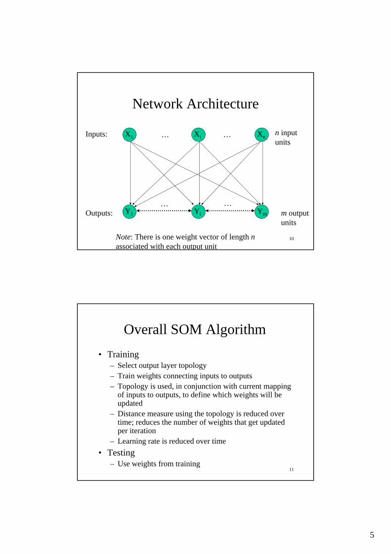
Conclusion
• Samples i1, i3 cluster with unit 2• Samples i2, i4 cluster with unit 1
29
What aboutgeneralization?
• New data samplei5: (1, 1, 1, 0)
• What unit should this cluster with?• What unit does this cluster with?
Training samplesi1: (1, 1, 0, 0)i2: (0, 0, 0, 1)i3: (1, 0, 0, 0)i4: (0, 0, 1, 1)
15
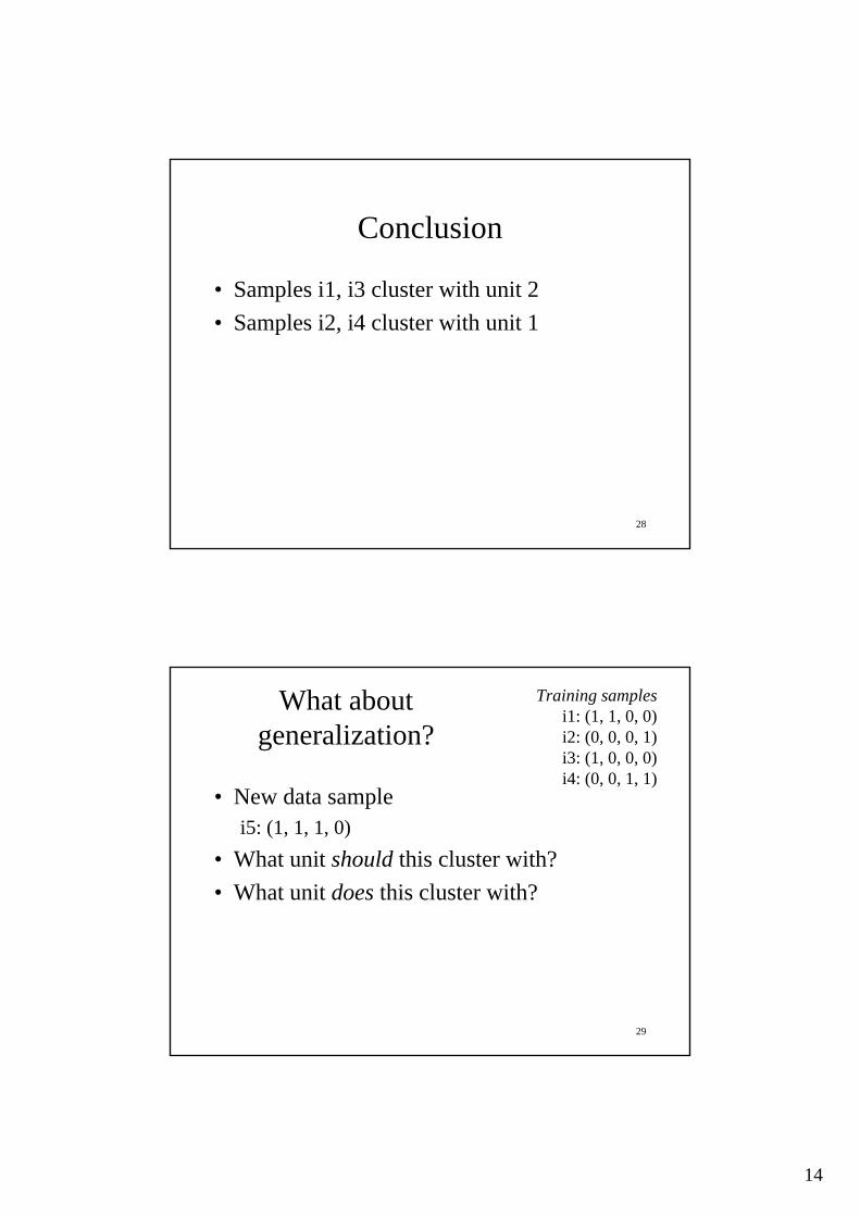
Example 5.7• pp. 191-194 of Mehotra et al. (1997)
111I60.50.50.5I5
001I41.50.50I3
000I21.81.71.1I1
Input Data Samples
• What do we expect as outputs from this example?
n = m = 3
B A C
Input units:
Output units
3100.7521.531.14I6
00.751.250.753.49I5
03.516.14I4
02.52.74I3
07.34I2
0I1
I6I5I4I3I2I1
Squared Euclidean Distancesof One Input Value to Another

16
32
111I6
0.50.50.5I5
001I4
1.50.50I3
000I2
1.81.71.1I1
ZYX
I2
I1I3
I4
I5
I6I1
I2
I3
I4
I5
I6
Data Samples Plotted as X,Y,Z points in 3D Space
33
Example Details:Neighborhood distance &
Learning Rate• Neighborhood distance
D(t) gives output unit neighborhood as a function of time0 <= t <= 6, D(t) = 1t > 6, D(t) = 0
• Learning rate also varies with time0 <= t <= 5, η(t) = 0.66 <= t <= 12, η(t) = .25t > 12, η(t) = 0.1
http://www.cprince.com/courses/cs5541/lectures/SOM/SOM.xls
Initial weightsWa 0.2 0.7 0.3Wb 0.1 0.1 0.9Wc 1 1 1

17
34
First Iteration
• Use input data in order I1, I2, …, I6– Start with I1: 1.1 1.7 1.8
• 1) Compute Euclidean distance of data from current weight vectors for output units
• 2) Compute weight updates
Initial weightsWa 0.2 0.7 0.3Wb 0.1 0.1 0.9Wc 1 1 1
B A C
35
Applying the SOM Algorithm
A0.10A18
B0.10B17
B0.10B16
C0.10C15
B0.10B14
C0.10C13
A0.250A12
B0.250B11
B0.250B10
C0.250C9
B0.250B8
C0.250C7
C, A0.51C6
A, B, C0.51A5
B, A0.51B4
A, B, C0.51A3
B, A0.51B2
C, A0.51C1
Weights Updated
η(t)D(t)654321time (t)
Data sample utilized
‘winning’ output node
B A C

18
Results: Classification & Weights
1, 3C
2, 4, 5B6A
Data sampleOutput node
Classification
1.340.950.61Wc0.30.230.47Wb
0.810.770.83Wa
Weights after 15 time steps
Weights after 21 time steps
1.3861.0250.659Wc0.26370.212670.46863Wb
0.8290.7930.847Wa
37
I1
I2
I3
I4
I5
I6
1.340.950.61Wc
0.30.230.47Wb
0.810.770.83Wa
111I6
0.50.50.5I5
001I4
1.50.50I3
000I2
1.81.71.1I1
ZYX
Data Samples & Weights Plotted as X,Y,Z points in 3D Space
I2
I1I3
I4
I5
I6
Wc
Wb
Wa
Wa
Wb
Wc

19
38
Another SOM example
• More typically, SOM’s are used with 2D topographies connecting the output units
• In this way, the final output can be interpreted spatially, i.e., as a map
39
Self-Organizing Colors• Inputs
– 3 input units: R, G, B– Randomly selected RGB colors
• Outputs– 2500 units– Connected in a 2D matrix– Amount neighbor weights changed
specified by a 2D Gaussian– Width of Gaussian decreases with
iterations of training
http://davis.wpi.edu/~matt/courses/soms/applet.html

20
40
SOM NetworkR G B
Fully-connected weights
50 units
50 units
Input: 3 units
Output: 2500 units
41
Algorithm modifications
• Random selection of winning output if multiple winning outputs
• Weight update modified to include a contribution factor
w j (t +1) = w j (t) +η(t)c(t,il ,w j (t))(il − w j (t))

21
42
Visualization
• Map weights onto colors
http://davis.wpi.edu/~matt/courses/soms/applet.html
43
U-matrix (Unified distance matrix)
• U-matrix representation of the Self-Organizing Map visualizes the distances between the neurons. The distance between the adjacent neuons is calculated and presented with different colorings between the adjacent nodes. A dark coloring between the neurons corresponds to a large distance and thus a gap between the codebook values in the input space. A light coloring between the neurons signifies that the codebook vectors are close to each other in the input space. Light areas can be thought as clusters and dark areas as cluster separators. This can be a helpful presentation when one tries to find clusters in the input data without having any a priori information about the clusters.
Figure: U-matrix representation of the Self-Organizing Map

22
44
U-Matrix Visualization
• Provides a simple way to visualize cluster boundaries on the map
• Simple algorithm:– for each node in the map, compute the average
of the distances between its weight vector and those of its immediate neighbors
• Average distance is a measure of a node’s similarity between it and its neighbors
45
U-Matrix Visualization
• Interpretation– one can encode the U-Matrix measurements as
grayscale values in an image, or as altitudes on a terrain
– landscape that represents the document space: the valleys, or dark areas are the clusters of data, and the mountains, or light areas are the boundaries between the clusters