MONETARY POLICY, INFLATION AND THE LEVEL OF...

149

MONETARY POLICY, INFLATION AND THE LEVEL OF ECONOMIC ACTIVITY IN BRASIL AFTER THE REAL PLAN: STYLIZED FACTS FROM SVAR MODELS

Brisne J. V. CéspedesElcyon C. R. LimaAlexis Maka

Originally published by Ipea in June 2005 as number 1101 of the series Texto para Discussão.

DISCUSSION PAPER

149B r a s í l i a , J a n u a r y 2 0 1 5

Originally published by Ipea in June 2005 as number 1101 of the series Texto para Discussão.

MONETARY POLICY, INFLATION AND THE LEVEL OF ECONOMIC ACTIVITY IN BRAZIL AFTER THE REAL PLAN: STYLIZED FACTS FROM SVAR MODELS

Brisne J. V. Céspedes1 Elcyon C. R. Lima2 Alexis Maka3

1. Ipea/Directorate of Rio de Janeiro.2. Ipea/Directorate of Rio de Janeiro and UERJ.3. Ipea/Directorate of Rio de Janeiro.

DISCUSSION PAPER

A publication to disseminate the findings of research

directly or indirectly conducted by the Institute for

Applied Economic Research (Ipea). Due to their

relevance, they provide information to specialists and

encourage contributions.

© Institute for Applied Economic Research – ipea 2015

Discussion paper / Institute for Applied Economic

Research.- Brasília : Rio de Janeiro : Ipea, 1990-

ISSN 1415-4765

1. Brazil. 2. Economic Aspects. 3. Social Aspects.

I. Institute for Applied Economic Research.

CDD 330.908

The authors are exclusively and entirely responsible for the

opinions expressed in this volume. These do not necessarily

reflect the views of the Institute for Applied Economic

Research or of the Secretariat of Strategic Affairs of the

Presidency of the Republic.

Reproduction of this text and the data it contains is

allowed as long as the source is cited. Reproductions for

commercial purposes are prohibited.

Federal Government of Brazil

Secretariat of Strategic Affairs of the Presidency of the Republic Minister Roberto Mangabeira Unger

A public foundation affiliated to the Secretariat of Strategic Affairs of the Presidency of the Republic, Ipea provides technical and institutional support to government actions – enabling the formulation of numerous public policies and programs for Brazilian development – and makes research and studies conducted by its staff available to society.

PresidentSergei Suarez Dillon Soares

Director of Institutional DevelopmentLuiz Cezar Loureiro de Azeredo

Director of Studies and Policies of the State,Institutions and DemocracyDaniel Ricardo de Castro Cerqueira

Director of Macroeconomic Studies and PoliciesCláudio Hamilton Matos dos Santos

Director of Regional, Urban and EnvironmentalStudies and PoliciesRogério Boueri Miranda

Director of Sectoral Studies and Policies,Innovation, Regulation and InfrastructureFernanda De Negri

Director of Social Studies and Policies, DeputyCarlos Henrique Leite Corseuil

Director of International Studies, Political and Economic RelationsRenato Coelho Baumann das Neves

Chief of StaffRuy Silva Pessoa

Chief Press and Communications OfficerJoão Cláudio Garcia Rodrigues Lima

URL: http://www.ipea.gov.brOmbudsman: http://www.ipea.gov.br/ouvidoria

DISCUSSION PAPER

A publication to disseminate the findings of research

directly or indirectly conducted by the Institute for

Applied Economic Research (Ipea). Due to their

relevance, they provide information to specialists and

encourage contributions.

© Institute for Applied Economic Research – ipea 2015

Discussion paper / Institute for Applied Economic

Research.- Brasília : Rio de Janeiro : Ipea, 1990-

ISSN 1415-4765

1. Brazil. 2. Economic Aspects. 3. Social Aspects.

I. Institute for Applied Economic Research.

CDD 330.908

The authors are exclusively and entirely responsible for the

opinions expressed in this volume. These do not necessarily

reflect the views of the Institute for Applied Economic

Research or of the Secretariat of Strategic Affairs of the

Presidency of the Republic.

Reproduction of this text and the data it contains is

allowed as long as the source is cited. Reproductions for

commercial purposes are prohibited.

JEL: E31; C32.

SUMMARY

SINOPSE

ABSTRACT

1 INTRODUCTION 1

2 BRAZILIAN STYLIZED FACTS AND VARs: A BRIEF REVIEW OF THE LITERATURE 2

3 ESTIMATION PROCEDURE AND DATA 3

4 “CONTEMPORANEOUS CAUSATION” AND THE IDENTIFICATION OF

STRUCTURAL VARs 4

5 CAUSAL INFERENCE AND THE SPIRTES-GLYMOUR-SCHEINES MODEL 6

6 MONETARY POLICY DEVELOPMENTS SINCE THE REAL PLAN 11

7 BENCHMARK MODEL AND RESULTS FOR THE FIRST SUBSAMPLE—1996/07-1998/08 15

8 BENCHMARK MODEL AND RESULTS FOR THE SECOND SUBSAMPLE—1999/03-2004/12 18

9 CONCLUDING REMARKS 20

BIBLIOGRAPHY 21

SINOPSEEste artigo investiga as relações estocásticas e dinâmicas de um grupo de variáveismacroeconômicas brasileiras (índices de preços, produção industrial, taxa de câmbionominal, taxas de juros de curto e médio prazo, e M1) para o período após o PlanoReal (1996-2004). Adota, como é usual na literatura, vários modelos SVARs (VARestruturais) para determinar os fatos estilizados relativos aos impactos de curto prazodas fontes exógenas de flutuação identificadas para esse grupo de variáveis.

O artigo inova ao empregar Grafos Acíclicos Direcionados (DAG) na obtenção dasrelações causais contemporâneas entre as variáveis e ao considerar que as alterações dapolítica monetária, ocorridas após o Plano Real, tornam essencial a divisão da nossaamostra em dois subperíodos (1996/07-1998/08 e 1999/03-2004/12).

Os resultados principais são: a) em resposta a uma inovação positiva na taxa de jurosde curto prazo (Selic), durante o subperíodo 1999-2004, a produção e o nível de preçoscaem — porém, a resposta da produção é mais rápida que a do nível de preços, que sóacontece com uma defasagem de aproximadamente quatro meses; b) para o período1996-1998, o efeito mais provável de uma inovação positiva na taxa de juros de curtoprazo é a redução do nível de preços também com uma defasagem de quatro meses,embora haja uma grande incerteza em relação a essa resposta e da produção; c) asinovações na taxa de juros de curto prazo (Selic) estão entre as fontes mais importantes daflutuação do nível de atividade econômica em ambos os subperíodos; e d) os choquesexógenos na taxa de câmbio e na taxa de juros de médio prazo (Swap Pré x CDI) são,para o período 1999-2004, as fontes mais importantes da flutuação da taxa de inflação.

ABSTRACTThis article investigates the stochastic and dynamic relationship of a group ofBrazilian macroeconomic variables (price and industrial production indexes, nominalexchange rate, short and medium-run nominal interest rates) for the period after theReal Plan (1996-2004). We adopt, as has become usual in the literature, severalSVAR (structural VAR) models to uncover stylized facts for the short-run impacts ofthe identified exogenous sources of fluctuations of this selected set of variables.

A distinctive feature of this article is the employment of Directed Acyclic Graphs(DAG) to obtain the contemporaneous causal order of the variables used to identifythe SVAR models. Another distinguishing characteristic is the careful attention paidto monetary policy developments after the Real Plan when splitting our sample intwo subsamples (1996/07-1998/08 and 1999/03-2004/12).

The main results are: a) in response to a positive short run interest rate innovation,during the 1999-2004 subperiod, the output and the price level decrease—however, theoutput response is faster and the price level responds with a lag of near four months; b)for the 1996-1998 subperiod, the most likely effect of a positive short run interest rateinnovation is the reduction of the price level (also with a four months lag), even thoughthere is a large uncertainty in this response, and the reduction of output; c)short runinterest rate innovations are one of the most important sources of temporary fluctuationsin the level of economic activity for both subsamples; and d) exogenous shocks to theexchange rate and to the medium term interest rate are for the 1999-2004 period, themost important sources of inflation rate fluctuation.

6 1

1 INTRODUCTIONThis article investigates the stochastic and dynamic relationship of a group ofBrazilian macroeconomic variables (price and industrial production indexes, nominalexchange rate, short and medium-run nominal interest rates) for the period after theReal Plan (1996-2004). We adopt, as has become usual in the literature, severalSVARs (structural VARs) models to uncover stylized facts for the short-run impactsof the identified exogenous sources of fluctuations of this selected group of variables.

There are many recent empirical studies about the dynamic relationship of setsof macroeconomic variables in Brazil employing SVARs as the framework of theiranalysis [Fiorencio, Lima and Moreira (1998), Rabanal and Schwartz (2001),Arquete and Jayme Jr. (2003) and Minella (2003), among others]. With theexception of Fiorencio, Lima, and Moreira (1998), all of them use Choleskydecompositions of the covariance of reduced form VAR disturbances to identify themodel. What distinguishes our article from the existing Brazilian literature is theadoption of a data oriented procedure to select over-identifying restrictions toestimate our SVARs. These restrictions follow from directed acyclic graphs (DAG)estimated by the TETRAD software developed by Spirtes, Glymour and Scheines(1993 and 2000) using as input the covariance of reduced form VAR disturbances.Another distinguishing characteristic of our article is the careful attention paid tomonetary policy developments after the Real Plan in the selection of the appropriatesubsamples. The first subsample goes from 1996/07 to 1998/08, the period withexchange rate “mini-bands” combined with the adoption of the TBC rate as aninformal target for the Selic rate. The second subsample goes from 1999/03 to2004/12, the period with free-floating exchange rate and explicit Selic targeting.

Over the last years there has been a growing interest on graphical models and inparticular on those based on DAGs as a general framework to describe and infercausal relations, exploring the connection between causal structure and probabilitydistributions [see, for example, Spirtes, Glymour and Scheines (1993 and 2000),Pearl (2000) and Lauritzen (2001)]. These methods have been used in a variety offields but are unfamiliar to most economists. Swanson and Granger (1997) were thefirst to apply graphical models to identify contemporaneous causal order of a SVAR,although they restrict the admissible structures to causal chains. Bessler and Lee(2002) use error correction and DAGs to study both lagged and contemporaneousrelations in late 19th and early 20th century United States data. Demiralp and Hoover(2003) evaluate the PC algorithm employed by TETRAD in a Monte Carlo studyand conclude that it is an effective tool of selecting the contemporaneous causal orderof SVARs. Awokuse and Bessler (2003) use DAGs to provide over-identifyingrestrictions on the innovations from a VAR and compare their results with the onesof Sims (1986). Moneta (2004) use DAGs and the data set of Bernanke and Mihov(1998) to identify the monetary policy shocks and their macroeconomic effects in theUnited States.

The main results are: a) in response to a positive short run interest rateinnovation, during the 1999-2004 subperiod, the output and the price leveldecrease—however, the output response is faster and the price level responds with alag of near four months; b) for the 1996-1998 subperiod, the most likely effect of a

2

positive short run interest rate innovation is the reduction of the price level (also witha four months lag), even though there is a large uncertainty in this response, and thereduction of output; c)short run interest rate innovations are one of the mostimportant sources of temporary fluctuations in the level of economic activity for bothsubsamples; and d) exogenous shocks to the exchange rate and to the medium terminterest rate are for the 1999-2004 period, the most important sources of inflationrate fluctuation.

The article is organized as follows. Section 2 presents a brief review of theBrazilian literature on macro variables and VARs. Section 3 describes the data andthe estimation procedures used. Section 4 explains how the identification ofcontemporaneous causation allows the identification of VARs. Section 5 presents theSpirtes-Glymour-Scheines Model. Section 6 describes monetary policy developmentsthat followed the Real Plan. Sections 7 and 8 present the benchmark model andresults for the first and the second subsamples, respectively. Finally, we offer someconcluding remarks on Section 9.

2 BRAZILIAN STYLIZED FACTS AND VARs: A BRIEF REVIEW OF THE LITERATUREIn this section we present a brief review of the recent Brazilian literature related toVARs and groups of macroeconomic variables.

Within the classical approach to VARs we have the studies of Rabanal andSchwartz (2001), Arquete and Jayme Jr. (2003), and Minella (2003), whileFiorencio, Lima and Moreira (1998) use a Bayesian VAR (BVAR) in their analysis.

Fiorencio, Lima and Moreira (1998) use BVAR models to analyze the impactsof monetary and exchange rate policies on unemployment and the price level afterthe Real Plan. The benchmark model was estimated for the period between January1991 and May 1997, with and without intervention on July and August 1994, usingas variables the price level (IPCA), the unemployment rate, the exchange rate, theinterest rate over capital financing (capital de giro) and the spread between capitalfinancing and private bonds (CDBs) rates. Employing a non-recursive identificationthey find that exchange rate shocks have significative impacts over the price level andunemployment and that monetary policy shocks do reduce the price level andincrease unemployment (in the model with intervention).1 According to them theresults suggest that there has been a change of regime after the Real Plan and that theeffects of economic policy shocks in the model are sensitive to the way this change ofregime is represented.

Rabanal and Schwartz (2001) use a VAR to analyze the effectiveness ofovernight interest rate (Selic) as a monetary policy instrument in Brazil and its effectson other interest rates, output, and prices for the period between January 1995 andAugust 2000. The variables included in the VAR are real output, inflation (IPCA),Selic rate, lending spreads, and money (M1), used in this order in the recursive

1. The impacts of monetary policy shocks over the price level and unemployment are reversed in the model withoutintervention.

6 3

(Cholesky) decomposition of the variance-covariance matrix of errors.2 Theyconclude that the Selic rate has a significant and persistent effect on output andlending spreads but interest rate shocks seemed to increase inflation “price puzzle”.

Arquete and Jayme Jr. (2003) evaluate the impact of monetary policy oninflation and output, covering the period between July 1994 and December 2002. Asvariables of the model they used inflation (IPCA), Selic rate, and output gap,employed in this order in the recursive decomposition of errors.3 In some of theiranalysis they also included a fifth variable (alternatively the nominal exchange rate,the real exchange rate, and the international reserves at the Central Bank) intended tocapture external constraints in Brazil. According to them monetary policy have realeffects, external restrictions and exchange rate volatility are important to the CentralBank reaction function but interest rate shocks increase inflation.

Minella (2003) investigates the macroeconomic relationships involving output,inflation, interest rate, and money, comparing three different periods: January1975/July 1985, August 1985/June 1994, September 1994/December 2000. Hisbenchmark model includes output, inflation (IGP-DI), nominal interest rate (Selicrate), and money (M1), used in this order in the Cholesky decomposition. His mainresults are that monetary policy shocks have significant effects on output but are notable to induce a reduction of inflation, with evidence suggesting the “price puzzle” inthe second subperiod.

3 ESTIMATION PROCEDURE AND DATAOur VARs reduced forms were estimated equation by equation using ordinary leastsquares (OLS). Following the results of Sims and Uhlig (1991) and Sims, Stock andWatson (1990) we do not performed unit root tests or cointegration analysis.

The models were estimated using monthly data divided into two subsamples:the first goes from 1996/07 to 1998/08 and second from 1999/03 to 2004/12.4 Thefollowing variables were selected to be part of the benchmark model: the Selic interestrate (short run rate fixed by the Brazilian Central Bank (BCB), annualized rate); thenominal exchange rate (end of period buying rate; source: BCB); the IPCA (officialprice index used for targeting inflation—source: IBGE); the 180 days Swap rate(PRE x CDI—annualized rate with 252 working days—basic source BM&F butcollected from http://www.risktech.com.br/); the Industrial Production index, usedas a proxy for output (source: IBGE); net foreign reserves (liquidity concept, asmeasured by the BCB); and a monetary aggregate (M1, working days average).

2. Another ordering is also analyzed: Selic rate, lending spreads, output, inflation, and money, but the results do notchange much.3. An alternative order analyzed was: output gap, inflation, Selic rate.4. The reasons for splitting the sample into two subsamples and the particular choice of dates are based on monetarypolicy developments and are discussed on Section 6.

4

4 “CONTEMPORANEOUS CAUSATION” AND THE IDENTIFICATION OF STRUCTURAL VARs

4.1 THE REDUCED FORM VAR MODEL

Let xt be the data vector—there are 5 variables in the model, therefore xt hasdimension 5x1—for each period t: xt = [ rt ,et pt rst Yt ]´, where: rt = Selic rate; et =exchange rate; pt = IPCA index; rst= swap rate (180 days); and Yt = industrialproduction index.

The reduced form VAR model is given by the following set of equations:

B(L) xt = µ + φ Zt +νt (1)

νt ∼ N (0, Σ) and E(νtν s' ) = 0, ∀ t ≠ s

where: B(L) = I – ∑ 31=i Bi L

i and L is the lag operator; Zt = seasonal dummies vector;

νt = reduced form residuals; and µ = constants’ vector.

This representation of the model does not allow for the identification of theeffects of exogenous independent shocks to the variables since the VAR reduced formresiduals are contemporaneously correlated (the Σ matrix is not diagonal).5 That is,the reduced form residuals (νt) can be interpreted as the result of linear combinationsof exogenous shocks that are not contemporaneously (in the same instant of time)correlated. It is not possible to distinguish whose exogenous shocks affect the residualof which reduced form equation. The residual can be the result, for example, of anexogenous and independent shock to the exchange rate, an exogenous andindependent shock to the interest rate, or a linear combination of both shocks. Inevaluations of the model (and of economic policies) it only makes sense to measureexogenous independent shocks. Therefore, it is necessary to present the model inanother form where the residuals are not contemporaneously correlated. A VARwhere the residuals are not contemporaneously correlated is called a structural VARand some of its equations have, in general, a behavioral interpretation. The same isnot true for reduced form VARs.

4.2 THE STRUCTURAL FORM VAR MODEL

The model in structural form is given by:

A(L) xt = ρ + θ Zt + εt (2)

εt ∼ N (0, D), D (diagonal)

and:

E (εtε s' ) = 0, ∀ t ≠ s

where: ρ = A0 µ, θ = A0 φ, A (L) = A0B(L), εt = A0 νt , A0 is a full rank matrix with eachelement in its main diagonal equal to 1.

5. These shocks are primitive and exogenous forces, with no common causes, that affect the variables of the model.

6 5

The relationships between the residuals εt and νt, and the covariances D and Σ,are given by:

νt = A(0)–1 εt or alternatively, νt = [I – A0 ] νt + εt (3)

A0 ΣA0´= D (4)

Given an estimate of A0 it is possible to estimate structural form parameters fromestimates of reduced form parameters. When the reduced form VAR is estimatedrestricting only the number of lags (chosen as the same in all equations and for allvariables), with no further restrictions, the structural VAR estimation proceeds in twosteps.6 In the first step the reduced form VAR is estimated and this comprise theestimation of the equation’s coefficients and of the covariance matrix of the reduced

form residuals ^Σ . In the second step the matrices A0 and D are estimated using only

the information given by the estimate of the covariance matrix of reduced formresiduals (estimated in the first step).

There are in general a large number of full rank matrices A0 and D (D diagonal)

that allow us to reproduce ^Σ . That is, there are several conditional dependency and

independency contemporaneous relations (“markov kernels”) between the variables—given by different specifications of which parameter in A0 is free and which is equal to0— that allow us to reproduce the partial correlations observed for the reduced formresiduals.7 In order to estimate the structural model it is necessary to identify anumber of conditional independence relations (that is, parameters equal to 0 in A0) tosatisfy the order condition for identification. Therefore, identifying A0 is equivalent toidentifying the conditional distributions (“Markov kernels”) of reduced formresiduals from information about their joint distribution. These conditionaldistributions can be interpreted either distributionally or causally. The causalinterpretation requires the knowledge that the conditional distributions wouldremain invariant under intervention.8 For SVARs to be useful, as we will show below,these conditional distributions must have a causal interpretation.

With A0 it is also estimated the orthogonal innovations of the structural formand identified the linear combinations between them that generate the reduced formresiduals [first version of equation (3)]. Alternatively, the residual of each reducedform equation in period t is modeled as the sum of a single innovation (an exogenous

6. This two step procedure can be adopted because the restrictions imposed to estimate the orthogonal residuals do notimply restrictions on the coefficients of the reduced form equations. They imply restrictions only on the variance of νt.7. The matrices A0 and D cannot have, together, a number of free parameters bigger than the number of free parametersin the symmetric matrix Σ. If n is the number of endogenous variables of the model then, to satisfy the order conditionfor identification of matrices A0 and D, it is necessary that the number of free parameters to be estimated in A0 be nobigger than n (n–1)/2 (matrix D is diagonal with n free parameters to be estimated). When n is smaller than n (n–1)/2the model is over-identified. There exists no simple general condition for local identification of the parameters of A0 andD. However, as has been shown by Rothenberg (1971), a necessary and sufficient condition for local identification of anyregular point in Rn is that the determinant of the information matrix be different from 0. In practice, evaluations of thedeterminant of the information matrix at some points, randomly chosen in the parameter space, is enough to establishthe identification of a certain model.8. For an interesting discussion of this topic, see Freedman (2004), Hausman and Woodward (1999), and Woodward(1997 and 2001).

6

structural shock independent of the other structural shocks),9 in period t, plus a linearcombination of the remaining reduced form shocks in the same period t [secondversion of equation (3)]. In this step it is thus important to establish a set ofcontemporaneous causal relations (conditional dependency and independencyrelations with a causal interpretation) between the reduced form residuals. That is, weneed to determine, for example, whether contemporaneously (within a month, if themodel uses monthly data) a shock to the reduced form residual of the exchange rateequation affects the reduced form residual of the interest rate, or the other wayaround, or whether there is bi-directional causality.

Obtaining stylized facts from VARs requires the identification of the structuralform model. The critical question is: is it possible to obtain these contemporaneouscausality relations, from the data, using just the contemporaneous correlation of thereduced form residuals, as summarized by their covariance matrix? We describe nexthow the methodology developed by Spirtes, Glymour and Scheines (1993 and 2000)[hereafter SGS] can help in the identification of the VAR structural form.

5 CAUSAL INFERENCE AND THE SPIRTES-GLYMOUR- SCHEINES MODEL

5.1 CAUSATION AND ASSOCIATION IN OBSERVATIONAL DATA

Common statistical wisdom dictates that causal effects cannot be consistentlyestimated from observational data (non-experimental data) alone unless one hassubstantial previous knowledge about the data generating mechanism. For this reasonthe contemporaneous causality restrictions, necessary for the identification ofstructural VARs, have been traditionally based on a priori restrictions, some of themarbitrary, others with some help of economic theory. However, SGS and Pearl andVerma (1991) claimed that it is possible to make causal inferences based onassociations observed in non-experimental data without previous knowledge.Moreover, if the causal relations can be represented by DAGs, SGS have shown thatunder some weak conditions—sufficient large sample and distribution of randomvariables “faithful” to the causal graph—there exist methods for identification ofcausal relations that are asymptotically (in sample size) correct. The results of SGS arediscussed in several articles [see, for example, Humphreys and Freedman (1996 and1999), Korb and Wallace (1997), Spirtes, Glymour and Scheines (1997), Robins andWasserman (1999), and Robins et al (2003)].

Robins and Wasserman (1999) use Bayesian methods to show that SGSimplicitly admit that, for the set of studied variables, the probability of nounmeasured common causes is positive and not small relative to the sample size. Ifthis is not true then causal relations cannot be identified using only data. They claimthat in studies with observational data, as those in economics and other areas, theassumption that this probability is small relative to the sample size, better reflects theposition of researchers. Robins et al (2003) use classical methods to analyze carefully

9. The exogenous shocks, in each period t, are represented by the vector εt. The VAR model is a formalization of therelationship between the vector εt and the vector of observed data xt. Employing the terminology adopted in the RealBusiness Cycle literature, the εt are “impulses” (or orthogonal innovations) and the matrices in A (L) [equation (2)],capture the propagation mechanism of the economy.

6 7

the asymptotic properties of SGS methodology. They show that in addition of beingasymptotically consistent, the procedures are pointwise consistent, although notuniform consistent. They also show that there exists no causality test, based onassociations of non-experimental data, which is uniform consistent (that is, for anyfinite sample, it is impossible to guarantee that the results of the proposed tests or anyother causality test will converge to the asymptotic results).10

In this article we abandon the classical criteria of uniform consistency [Robins etal (2003)] and implicitly adopt Bayesian consistency criteria. That is, we assume thatthe probability of no unmeasured common causes, for the set of variables analyzed, ispositive and not small relative to the sample size. This assumption justifies our use ofthe procedures proposed by SGS. Nevertheless, we agree with the view that thishypothesis maybe too strong and that the search for a more robust method, toidentify matrix A0, should continue. We believe the economic theory, in its presentstage, does not establish a set of fully acceptable restrictions that allows for theidentification of A0. One possible extension of the present work would be to developBayesian estimation methods, similar to the ones proposed by Robins andWasserman (1999), that would allow for the combination of prior information andthe information in the data.

The SGS procedures allow us to establish the conditional independence relationsthat are equivalent to determining whose coefficients of matrix A0 are equal to 0. Theframework developed by SGS does not rule out the possibility of finding alternativesets of conditional independence relations for a given data set. In this case we arriveat a set of matrices A0 that are observationally equivalent. It may be the case that thefound conditional independence relations are not enough to allow for theidentification of the matrices. However, in all applications of the methodology wefound at most two alternative matrices A0 and the implied restrictions were enough toarrive at an over-identified model.

5.2 THE SPIRTES-GLYMOUR-SCHEINES MODEL

We present below a brief description of the SGS model taken from Robins et al(2003).

A (causal) directed graph is a picture that represents a causal flow, indicated byarrows (directed edges) between some pair of vertices (variables). An edge in a graphcan be either directed (marked by a single arrowhead on the edge) or undirected(unmarked). If all edges of a graph are directed, we say that it is a directed graph.Arrows represent causal relationships: if there is an arrow pointing from Xi to Xj itmeans that Xi has a direct causal effect on Xj, relative to all vertices. A directed path oflength n between vertices X and Y is a sequence of n vertices starting at X and endingat Y of the form X → V1→ V2 →…→ Vn–2 → Y or of the form X ←V1←V2←…←Vn-2

←Y. A DAG11 is a directed graph with no directed cycle, in that one cannot start at avertex (variable) and follow a directed path back to that vertex. The vertex Xi is in theset of “parents” of a variable Xj in a DAG G, denoted by PAG(Xj), if there is an edge

10. It is important to point out that these negative results apply to any method, not just to SGS methodology. No kind ofsearch, no kind of model selection, no kind of test (like the t-test), can get around these limitations. Nor can any informalmethod based on human judgment or insight escape these limitations.11. References on DAG include Lauritzen (1996) and Pearl (2000).

8

Xi→Xj in G. Xj is a “descendent” of Xi in G if there is a directed path from Xi to Xj orXi = Xj.

The SGS model begins with a triple <G, V, P>, where G is a DAG with a non-empty set of vertices (variables) VV= (X1, X2,…, Xk) is a vector of randomvariablesand P is a joint probability distribution for V. It is also used the CausalMarkov Condition and the assumption that P is “faithful” to G. These two conceptsand some auxiliary concepts are defined below.

Definition (Distribution Markov to G or “compatible” with G): A distributionP with density function p is “Markov” to G if p(x1,....,xk) = ∏

=

k

i 1

p{xi | paG(xi)}, where

p{xi | paG(xi)} = p(xi) when paG(xi)} = ∅. This formula is called the “Markovfactorization” of P according to G.

Let P (G) be all distributions that are Markov to G. If P is in P (G) then P is“compatible” with G.

The next proposition was first stated in Pearl and Verma (1991), but it isimplicit in the works of Kiiveri, Speed and Carlin (1984) and others.

Proposition 1

The Causal Markov Condition: Any Distribution Generated by a Markovian Model G isMarkov to G12

A model is “Markovian” [Pearl (2000)] if it can be represented by a DAG and all theerror terms are jointly independent. The Causal Markov Condition states that if Grepresents the data generating mechanism for P, and G is Markovian, then P ∈ P (G). Asimple proof of Proposition 1 is given in Pearl (2000, p. 30).

Let P ∈ P (G) and let ϕ(P) represent all independence and conditionalindependence relations that hold for the variables in V under P. Let ϕG be allindependence and conditional independence relationships that are common to all thedistributions in P (G).

Definition (faithfulness) P is “faithful” to G if ϕ(P) = ϕG.

Therefore P is faithful if it does not possess extra independence relationships notshared by all the other distributions in P(G). As Spirtes-Glymour-Scheines say: “theFaithfulness Condition can be thought of as the assumption that conditionalindependence relations are due to causal structure rather [than] to accidents ofparameters values”.

A convenient way of characterizing the set of distributions that belongs to P (G)is to list the set of all independence and conditional independence relations thatbelongs to ϕG. These independencies can be read off G using a graphical criterioncalled d-separation [where d stands for directional, Pearl (1988)]. Consider threedisjoint sets of variables X, Y, and Z, which are represented as vertices in G. To testwhether X is independent of Y given Z in any distribution that belongs to P (G), weneed to test whether the vertices corresponding to variables Z “block” all paths fromvertices in X to vertices in Y. Blocking is to be interpreted as stopping the flow of

12. For a discussion of the concept of causality used here (due to Judea Pearl and others) see Woodward (2001).

6 9

information (or of dependency) between the variables that are connected by suchpaths, as defined next.

Definition (d-separation): A path p is said to be d-separated (or blocked) by a setof vertices Z if and only if:

1. p contains a chain jmi →→ or a fork jmi →← such that the middlevertex m is in Z; or

2. p contains an inverted fork (or collider) jmi ←→ such that the middlevertex m is not in Z and such that no descendant of m is in Z.

A set Z is said to d-separate X from Y if and only if Z blocks every path from avertex in X to a vertex in Y.

FIGURE 1

1X

2X 3X

4X

5X

In Figure 1, X={ 2X } and Y={ 3X } are d-separated by Z={ 1X }, because both

paths connecting 2X and 3X are blocked by Z. The path 312 XXX →← isblocked because it is a fork in which the middle vertex 1X is in Z, while the path

342 XXX ←→ is blocked because it is an inverted fork in which the middle vertex

4X and all its descendants are outside Z. However, X and Y are not d-separated by

the set Z´={ 1X , 5X }: the path 342 XXX ←→ (an inverted fork) is not blocked by

Z´, since 5X , a descendant of the middle vertex 4X , is in Z´.

In order to distinguish between the probabilistic notion of conditionalindependence and the graphical notion of d-separation, we will use ( )

PZYX | | to

denote the independence of X and Y given Z in the former notion and ( )G

ZYX | | for the later notion. The following proposition due to Verma and Pearl (1988) andGeiger, Verma and Pearl (1990) shows that there is a one-to-one correspondencebetween the probabilistic and graphical notions of conditional independence:13

13. For a sketch of the proof see Pearl (2000).

10

Proposition 2

For Any Three Disjoint Subsets of Vertices (X, Y, Z) in a DAG G and for allProbability Functions P, we have:

a) ( ) ( )PG

ZYXZYX | | | | ⇒ , whenever P ∈ P(G); and

b) if ( )P

ZYX | | holds in all distributions in P(G) (faithfulness), then it follows

that ( )P

ZYX | | ⇒ ( )G

ZYX | | .

SGS developed algorithms, for inferring causal relations from data, that areembodied in computer program used in this paper, called TETRAD.14 The programtakes as input the joint distribution of the variables and its output is a set of DAGsover these variables that are observationally equivalent.15 TETRAD can handle twokinds of sample data: a) independent, identically distributed multivariate Gaussianobservations, or, b) independent, identically distributed multinomial observations. Inthe identification of SVARs TETRAD uses as input the covariance matrix of reducedform VAR residuals.

In our application TETRAD begins with a “saturated” graph, where any pair ofnodes (variables) are joined by an undirected edge. If the null hypothesis of 0conditional correlation cannot be rejected—at, say, the 5% level, using Fisher’s ztest—the edge is deleted.16 After examining all pair of vertices, TETRAD move on totriples, and so forth. TETRAD also orients the edges left in the graph.

5.3 DAGS AND THE IDENTIFICATION OF STRUCTURAL VARS

Next we show how DAGs can be used to impose restrictions that allows for theidentification of SVARs. In the example below we assume that the VAR has fourendogenous variables.

The relationship between reduced form and structural form residuals in a VARis given by equation (3):

νt = [I – A0 ] νt + εt

where: νt = column vector, with dimension 4x1, with reduced form VAR residuals atperiod t;

εt = column vector, with dimension 4x1, with structural form VAR residual atperiod t; and

A0 = full rank matrix with the relationship between the two types of residuals.

The above equations are a system of linear equations, where each variable(reduced form residual) is a linear function of its direct causes and an error term

14. The program is available for download at www.phil.cmu.edu/projects/tetrad/index.html. We used TETRAD III in thispaper.15. Two linear-normal recursive SEMs are observationally equivalent if and only if they entail the same sets of 0 partialcorrelations.16. Based on simulation tests with random DAGs, SGS suggests setting the significance level at 20% for sample sizesmaller than 100; at 10% for sample size between 100 and 300; and at 0.5% (or smaller) for larger samples. Wefollowed their suggestion and set the significance level at 20%.

6 11

(structural residual), with error terms independent of each other. If the graph G thatrepresents the model has no cycles (is a DAG) then the variables are generated by aMarkovian model. Therefore, the model satisfy the property that guarantees thecompatibility between its distribution function and graph G.17 Because conditionalindependence implies 0 partial correlation, Proposition 2 translates into a graphicaltest for identifying those partial correlations that must vanish in the model.18

Therefore, equations (3) can be structured according to a DAG G, and the partialcorrelation coefficient 3V.2V1Vρ vanishes whenever the vertices corresponding to thevariables in V3 d-separate vertex V1 from vertex V2 in G.

We present below an example of the relationship between a DAG (the graphbelow), equation (3) and the coefficients that are considered different from 0 in A0:

19

FIGURE 2

v1(t) = ε1(t)v2 (t) = ε2(t)v3(t) =-A31v1(t) −Α32v2(t)+ε 3(t)v4(t) =-A43v3(t) +ε4(t)

v1

ε1

v2

v3 v4

ε2

ε3 ε4

=

1000100100001

43

32310

AAA

A

6 MONETARY POLICY DEVELOPMENTS SINCE THE REAL PLAN20

The Real Plan introduced several changes in the rules of monetary policy to achieveinflation stabilization. The Provisional Measure (PM) 566 of July 29th of 1994, whichimplemented these changes, established quarterly limits for money expansion

17. For a sketch of the proof see Pearl (2000).18. The partial correlation coefficient of X and Y, controlling for Z is given

by 2/12/1. )1()1/()( YZXZYZXZXYZXY ρρρρρρ −−−= .

19. εi is the structural error term of equation i (i = 1, 2, 3, 4).20. As source of information this section used Lopes (2003), several issues of the Boletim do Banco Central do Brasil forthe period, the provisional measures cited in the text, Central Bank of Brazil (1999), the IMF Survey (Nov. 1998), theBoletim de Conjuntura IPEA (Jan. 1999), as well as information contained in the homepage of the Central Bank of Brazil(www.bcb.gov.br).

12

in the new currency, the real.21 Starting in the first quarter of 1995 the procedure ofsetting monetary limits was substituted for a monetary programming with quarterlyprojections for the expansion of monetary base (restricted and extended), M1, and M4(the broadest monetary aggregate), formulated by the Central Bank and submitted to theCongress for evaluation, after approval by the National Monetary Council (CMN).

Although the new currency (the Real) was introduced at a rate of one-to-one to theUnited States dollar, there was no official commitment to any exchange rate policy. Atfirst the Central Bank did not intervene in the foreign currency market and the Realappreciated vis-à-vis the dollar. The Central Bank reports that it began intervening in theexchange rate market in the second half of September [see Central Bank of Brazil (1999)]On March 10th of 1995 the Central Bank introduced a formal 0.88-0.93 exchange rateband with the commitment to intervene only on its limits, after an unsuccessful attemptto introduce a narrower band a day before when it lost US$ 4 billion in internationalreserves (see Figure 3). At the same time the Selic interest rate was sharply increased inorder to prevent any speculation against the real (see Figure 4).

On June of 1995 a new 0.91-0.99 exchange rate band was announced togetherwith the introduction of a new mechanism of intervention in the foreign exchangemarket, the “spread-auction”, that in practice resulted in an exchange rate peg (seeFigure 5) through what became know as “mini-bands”.22 There was no official rulefor the speed of the crawling but it was understood that it was being set so as toslowly devaluate the real.

On June 20th of 1996 the Monetary Policy Committee (Copom) was createdwith the objective of setting the stance of monetary policy and the short-term interestrate. The design of monetary policy operational procedure was modified with theintroduction of two new interest rates—the TBC and the TBAN.23 According toLopes (2003), in this setup inspired in the Deutsche Bundesbank the TBC, the rateat which banks could have financial assistance through rediscount window of theCentral Bank, played the role of an interest rate floor, and the TBAN the ceiling. Inprinciple, the Selic rate would be allowed to fluctuate freely inside this interest rateband, with the values of both TBC and TBAN rates being determined by theCopom. However, in practice the Central Bank managed to put the Selic rate closeto the TBC rate most of the time (see Figure 6).

21. The ceilings for monetary base in the third and fourth quarters of 1994 were set at R$ 7,5 billion and R$ 8,5 billion,respectively. However, the same PM allowed the CMN to authorize an extra margin of up to 20% of these limits. Neitherthe PM 566 nor the PM 596 (its update), defined how the monetary ceilings should be measured. This was set asresponsibility of the CMN, who later chose the daily average balance concept. In the July-September quarter themonetary base—measured by average daily balances—reached R$ 8.9 billion, slightly below the R$ 9 billion ceilingonce the 20% extra margin was approved by the CMN on August 24th [the monetary base measured by end of periodbalances reached R$ 12,8 billion at the end of the third quarter of 1994]. The monetary limit for the last quarter of 1994was reviewed twice. The PM 681 of October 27th of 1994 substituted the original limit of R$ 8,5 billion substituted by anew limit that allowed an increase of 13.33% over the balances observed at the end of September, meaning that thenew limit was R$ 14,5 billion. Then, on December 21st the CMN approved a new ceiling of R$ 15,1 billion. The averagedaily balance of the monetary base of the October-December quarter reached R$ 14,8 billion. The PM 681 alsointroduced the concept of extended monetary base together with the establishment of a 0 growth rate for it during thelast quarter of 1994 [the extended base adds federal government securities in the market (except LBC-E) to thetraditional concept of monetary base]. The CMN authorized on December 21st a growth rate of 3.5% for the extendedbase, whose effective growth reached 1.9%.22. Notice that the “mini-bands” are not pictured in Figure 5, only the “regular” bands.23. The TBC was created on July 1st of 1996 and the TBAN on August 28th of 1996.

6 13

FIGURE 3INTERNATIONAL RESERVES, FROM JULY 1994 TO FEBRUARY 1999. (NOTE: THE AMOUNTS PICTUREDABOVE INCLUDE US$ 9.3 BILLION RECEIVED ON DECEMBER 1998 AS PART OF THE FINANCIALPROGRAM COORDINATED BY THE IMF)

0

10

20

30

40

50

60

70

80

july/9

4

sept/

94

nov/9

4jan

/95

mar/95

may/95

july/9

5

sept/

95

nov/9

5jan

/96

mar/96

may/96

july/9

6

sept/

96

nov/9

6jan

/97

mar/97

may/97

july/9

7

sept/

97

nov/9

7jan

/98

mar/98

may/98

july/9

8

sept/

98

nov/9

8jan

/99

US$

bill

ion

FIGURE 4SELIC OVERNIGHT INTEREST RATE, ANNUALIZED

15

25

35

45

55

65

75

85

01/0

8/94

01/1

0/94

01/1

2/94

01/0

2/95

01/0

4/95

01/0

6/95

01/0

8/95

01/1

0/95

01/1

2/95

01/0

2/96

01/0

4/96

01/0

6/96

01/0

8/96

01/1

0/96

01/1

2/96

01/0

2/97

01/0

4/97

01/0

6/97

01/0

8/97

01/1

0/97

01/1

2/97

01/0

2/98

01/0

4/98

01/0

6/98

01/0

8/98

01/1

0/98

01/1

2/98

01/0

2/99

%

FIGURE 5EXCHANGE RATE (R$/US$), FROM JULY 1994 TO JANUARY 1999

��

��

��

��

0,8

0,85

0,9

0,95

1

1,05

1,1

1,15

1,2

1,25

01/0

7/94

01/0

9/94

01/1

1/94

01/0

1/95

01/0

3/95

01/0

5/95

01/0

7/95

01/0

9/95

01/1

1/95

01/0

1/96

01/0

3/96

01/0

5/96

01/0

7/96

01/0

9/96

01/1

1/96

01/0

1/97

01/0

3/97

01/0

5/97

01/0

7/97

01/0

9/97

01/1

1/97

01/0

1/98

01/0

3/98

01/0

5/98

01/0

7/98

01/0

9/98

01/1

1/98

01/0

1/99

Exchange Rate

��Band Lower Limit Band Upper Limit

14

FIGURE 6OVERNIGHT INTEREST RATES, ANNUALIZED – FROM JULY 1996 TO MARCH 1999

��

��

��

��

��

��

��

��

��

��

15

20

25

30

35

40

45

50

55

01/0

7/96

01/0

8/96

01/0

9/96

01/1

0/96

01/1

1/96

01/1

2/96

01/0

1/97

01/0

2/97

01/0

3/97

01/0

4/97

01/0

5/97

01/0

6/97

01/0

7/97

01/0

8/97

01/0

9/97

01/1

0/97

01/1

1/97

01/1

2/97

01/0

1/98

01/0

2/98

01/0

3/98

01/0

4/98

01/0

5/98

01/0

6/98

01/0

7/98

01/0

8/98

01/0

9/98

01/1

0/98

01/1

1/98

01/1

2/98

01/0

1/99

01/0

2/99

01/0

3/99

%

��TBC SELIC TBAN

Note: the TBC rediscount window was closed from September 4th of 1998 to December 16th of 1998.

The Asian Crisis24 and the Russian default25 affected Brazil through the loss ofinternational reserves, which caused sharp interest rate increases on October 1997and September 1998. The monetary policy during these periods was dominated bythe Brazilian government attempt to defend the real. On September 4th, 1998 therewas a change in the operational procedure of the Central Bank: the rediscountwindow at the TBC rate was closed, making the Selic rate jump to the TBAN rate.Despite the government’s efforts, the international reserves kept sliding. OnNovember 13th, 1998 Brazil and the International Monetary Fund (IMF) announcedthe conclusion of negotiations on a financial program that provided support of US$41.5 billion over the next three years, making US$ 37 billion available, if needed,over the next 12 months. The Central Bank gave up defending the exchange rate onJanuary 15th, 1999 and announced the free-floating as the new exchange rate regimeon January 18th, 1999.

On March 4th of 1999 both TBC and TBAN rates were extinguished and theCentral Bank started a new monetary policy operational procedure of targeting theSelic rate, with its value been determined by the Copom. Since 1996, the Copom'scomposition and objectives, and the frequency of its meetings, have undergone anumber of changes. Brazil implemented a formal inflation targeting framework formonetary policy on June 21 of 1999. Under the inflation targeting regime, theCopom's monetary policy decisions have as their main objective the achievement ofthe inflation targets set by the CMN. If inflation breaches the target set by the CMN,

24. In the wake of the Asian Crisis Brazil lost near 15% of its foreign reserves on October 28th of 1997 (see Figure 3). Inresponse, the Central Bank increased sharply interest rates with the Selic overnight rate reaching more than 45% perannum (it was near 20% before, see Figure 6) and started to operate in the dollar futures market in order to defend theexchange rate. Despite the negative effect of the interest rate hike over the public debt, it induced a huge increase ininternational reserves, which moved from US$ 52 billion in November 1997 to near US$ 75 billion in April 1998 (seeFigure 3).25. On August 17th of 1998, the rouble devaluation and the Russian default provoked an international financial crisis.According to Lopes, the Central Bank responded increasing interest rates in four stages (see Figure 6). First, onSeptember 2nd, the TBAN rate was increased from 25.75% to 29.75% per annum. In the second stage, on September 4th,the rediscount window at the TBC rate was closed, making the Selic rate jump to the TBAN rate. In the third stage, onSeptember 4th, the TBAN rate was increased to 49.75%. In the last stage, the Selic rate was gradually increased throughopen market operations, reaching 42.75% on November 4th.

6 15

the Governor of the Central Bank is required to write an open letter to the Ministerof Finance explaining the reasons why the target was missed, as well as the measuresrequired to bring inflation back to the target, and the time period over which thesemeasures are expected to take effect. The Selic target is fixed for the period betweenregular Copom meetings. The Copom can also establish a monetary policy bias at itsregular meetings; a bias (to ease or tighten) authorizes the Central Bank's Governorto alter the Selic interest rate target in the direction of the bias at anytime betweenregular Copom meetings.

As seen above, Brazil experienced several changes in policy regime in the periodafter the Real Plan. Therefore, in order to appropriately conduct an empirical analysisof this period it is important to divide it in subsamples sharing common features.Unfortunately, some of these subsamples are too short to allow for any type ofeconometric analysis. Based on the exchange rate regime and monetary policyoperational procedures, we decided to partition our sample into two subsamples. Thefirst one goes from 1996/07 to 1998/08, the period with exchange rate “mini-bands”combined with the adoption of the TBC rate as an informal target for the Selic rate.The second one goes from 1999/03 to 2004/12, the period with free-floatingexchange rate and explicit Selic targeting.

7 BENCHMARK MODEL AND RESULTS FOR THE FIRST SUBSAMPLE—1996/07-1998/08The variables selected for the Benchmark Model of the first subsample are: Selic,international reserves, price level, money (M1), output, a constant, and seasonaldummies. The chosen lag length of the model is one, following the SchwarzInformation Criterion (SIC).

7.1 CONTEMPORANEOUS CAUSAL ORDERING

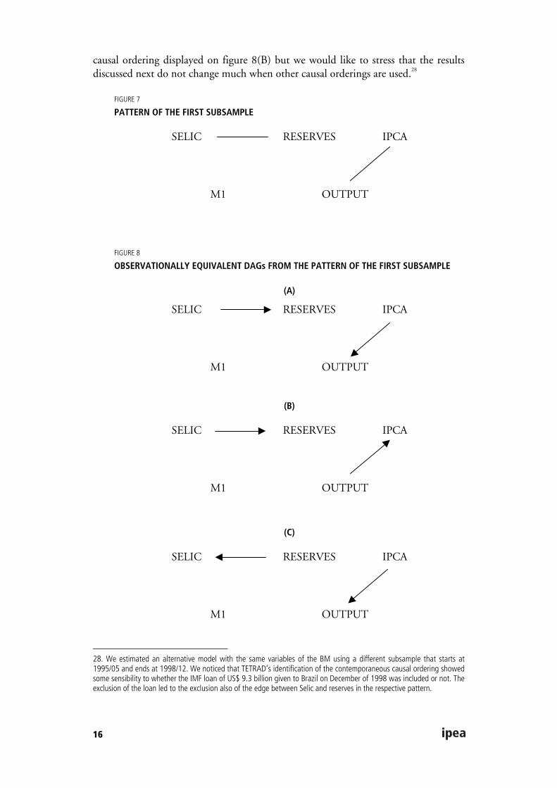
Applying TETRAD at the 20% significance level and assuming that the variablesselected for the model are causally sufficient,26 we obtain what is known as a pattern,27

shown in Figure 7. The pattern is a graphical representation of the set ofobservationally equivalent DAGs containing the contemporaneous causal ordering ofthe variables. According to Figure 7 the Benchmark Model (BM) has fourobservationally equivalent DAGs, displayed on Figure 8. Each of these DAGs is avalid representation of the contemporaneous causal ordering of the BM of the firstperiod according to TETRAD. In what follows we will restrict our attention to the

26. A set of variables V is said to be causally sufficient if every common cause of any two or more variables in V is in V.TETRAD has a bias towards excluding causal relations present in the data, to overcome this problem it is suggested thata 20% significance level be used.27. A pattern is a partially oriented DAG, where the directed edges represent arrows that are common to every memberin the equivalent class, while the undirected edges are directed one way in some DAGs and another way in others.Undirected edges mean that there is causality in one of the two directions but not on both, while double oriented edges(↔) mean causality on both directions.

16

causal ordering displayed on figure 8(B) but we would like to stress that the resultsdiscussed next do not change much when other causal orderings are used.28

FIGURE 7

PATTERN OF THE FIRST SUBSAMPLE

SELIC RESERVES IPCA

M1 OUTPUT

FIGURE 8

OBSERVATIONALLY EQUIVALENT DAGs FROM THE PATTERN OF THE FIRST SUBSAMPLE

(A)

SELIC RESERVES IPCA

M1 OUTPUT

(B)

SELIC RESERVES IPCA

M1 OUTPUT

(C)

SELIC RESERVES IPCA

M1 OUTPUT

28. We estimated an alternative model with the same variables of the BM using a different subsample that starts at1995/05 and ends at 1998/12. We noticed that TETRAD’s identification of the contemporaneous causal ordering showedsome sensibility to whether the IMF loan of US$ 9.3 billion given to Brazil on December of 1998 was included or not. Theexclusion of the loan led to the exclusion also of the edge between Selic and reserves in the respective pattern.

6 17

(D)

SELIC RESERVES IPCA

M1 OUTPUT

7.2 IMPULSE RESPONSE ANALYSIS

Using the contemporaneous causal ordering of Figure 8(B) to identify the BM, wecompute and analyze in this section the impulse response functions of economicvariables to exogenous and independent shocks.29

The impulse response functions (IRF) displayed on Figure 930 show that outputand money fall in response to a Selic shock. The large uncertainty of the response ofthe price level to a Selic shock (reflected in large probability bands) is not surprising,due to the small sample size, and indicates that we should be cautious when inferringwhat is the response of the price level to a Selic shock. However, the most likelyresult (indicated by the solid line between the bands) is that the price level goes downin response to a Selic innovation.31 Money shocks on the other side have a moreimmediate effect over prices but no significant effect on the Selic rate (this is calledliquidity puzzle). International reserves shocks decrease interest rates and stimulateeconomic activity, leading to an increase in inflation. Therefore, in this period theSelic shock is the better candidate for a monetary policy shock.

29. We will not present and discuss the parameters estimates of the model because of the difficulties associated withtheir interpretation, specially the estimates of the Central Bank reaction function. For a discussion of the pitfalls ininterpreting estimated monetary policy rules, see Christiano et al (1999).30. The error bands for impulse responses were constructed following the methodology suggested by Sims and Zha(1999).31. In an alternative model for the 1995/05-1998/12 subperiod, where the exchange rate and the Swap rate were usedinstead of international reserves and M1, we observed an increase in the price level in response to a Selic shock, withouttaking into account the uncertainty of the period.

18

FIGURE 9IRFs OF THE BENCHMARK MODEL 1996/07-1998/08, WITH 50% PROBABILITY BANDS

q¤©¨¢

P R T V ON OPKSNSONOS

³>ONKQq¤©¨¢


³>ONKQp¤®¤�±¤®


³>ONKQgna_F�¨¢¤>¨«£¤³G


³>ONKQkO


³>ONKQ

>g«£°®¯�¨ ©>�¬£°¢¯¨¬«

p¤®¤�±

¤®

P R T V ON OP

KNLNP

N

NLNP

NLNR

P R T V ON OP

KNLNP

N

NLNP

NLNR

P R T V ON OP

KNLNP

N

NLNP

NLNR

P R T V ON OP

KNLNP

N

NLNP

NLNR

P R T V ON OP

KNLNP

N

NLNP

NLNR

>>>>>>>>>>>>gn

a_

>F�¨¢¤>¨«£¤³G

P R T V ON OP

KP

KO

N

O

³>ONKQ

P R T V ON OP

KP

KO

N

O

³>ONKQ

P R T V ON OP

KP

KO

N

O

³>ONKQ

P R T V ON OP

KP

KO

N

O

³>ONKQ

P R T V ON OP

KP

KO

N

O

³>ONKQ

kO

P R T V ON OP

KNLNR

KNLNP

N

P R T V ON OP

KNLNR

KNLNP

N

P R T V ON OP

KNLNR

KNLNP

N

P R T V ON OP

KNLNR

KNLNP

N

P R T V ON OP

KNLNR

KNLNP

N

>>g«

£°®¯�

¨ ©

>�¬

£°¢¯¨¬«

P R T V ON OP

KON

KS

N

³>ONKQ

P R T V ON OP

KON

KS

N

³>ONKQ

P R T V ON OP

KON

KS

N

³>ONKQ

P R T V ON OP

KON

KS

N

³>ONKQ

P R T V ON OP

KON

KS

N

³>ONKQ

p¤®¬«®¤>¬

¥

q§¬¢&>¯¬

8 BENCHMARK MODEL AND RESULTS FOR THE SECOND SUBSAMPLE—1999/03-2004/12The variables selected for the BM of the second subsample are not all the same asthose chosen for the first period. The differences are that we substituted internationalreserves for the exchange rate, given that now there is free floating, and substitutedmoney for medium term interest rate (Swap) because the Central Bank startedtargeting (explicitly) the interest rate. Therefore, the BM is now composed by: Selic,exchange rate, price level, Swap, output, a constant, and seasonal dummies. Thechosen lag length of the model is two, following, as in the first period, the SIC.

8.1 CONTEMPORANEOUS CAUSAL ORDERING

Using TETRAD to find out the contemporaneous causal ordering of the BM of thesecond subsample, we obtain the pattern displayed on Figure 10, containing just oneDAG.32 At this point we assume that monetary policy cannot respondcontemporaneously to disturbances in output, due to the absence of contemporarydata of output at the time policy decisions have to be made.33 Running TETRADagain imposing the assumption that output cannot affect contemporaneously Selic,we get a new pattern shown in Figure 11 displaying the contemporaneous causal

32. Remember that double oriented edges (↔) mean causality in both directions.

33. This assumption is part of the identifying restrictions made, for example, by Sims and Zha (1996).

6 19

ordering used to identify the BM of the second subsample. With this identificationwe obtained the IRFs of the BM of the second subsample, discussed next.34

FIGURE 10INITIAL PATTERN

SELIC EXCHANGE RATE IPCA

SWAP OUTPUT

FIGURE 11PATTERN OBTAINED AFTER IMPOSING THE IDENTIFYING RESTRICTION THAT MONETARY POLICY CANNOTRESPOND CONTEMPORANEOUSLY TO DISTURBANCES IN OUTPUT

SELIC EXCHANGE RATE IPCA

SWAP OUTPUT

8.2 IMPULSE RESPONSE ANALYSIS

As can be seen in Figure 12, the responses to a Selic innovation are in line with theresults that one would expect from monetary policy shocks: the price level goesdown, output decreases, and there is an exchange rate appreciation. It is interesting tonote the lag with which the price level responds to a Selic shock: it takes near fourmonths until the IPCA starts to fall, despite the immediate contraction of economicactivity. Swap shocks have effects similar to monetary policy shocks and one possibleexplanation for this is that the Swap rate is anticipating movements in the Selic ratethat cannot be inferred by the chosen set of variables.

Exchange rate shocks induce an immediate increase in the Swap rate togetherwith a reduction in the level of economic activity. After a period of near five months,inflation starts to increase in response to the persistent exchange rate depreciation,despite the immediate increase in the Swap rate and the increase in the Selic rate fourmonths after the shock. In fact, exogenous shocks to the exchange rate and to theSwap rate are for the 1999-2004 period, the most important exogenous sources ofinflation rate fluctuation.

The increase in the price level in response to output shocks suggests that they areassociated with demand shocks. This inflationary effect together with exchange ratedevaluation explain why interest rates goes up in response to output shocks duringthe second subsample.

34. We would like to point out that the behavior of the IRFs does not change much if the initial pattern (Figure 10) isused to identify the BM.

20

We estimated alternative models using the same variables of the BM employingdifferent lag lengths (lags 1, 3, 4, 5). Using TETRAD to identify each model withoutimposing any additional identifying restriction, we computed the respective IRFs(without error bands). Of these IRFs, only those associated with the model with lag 1didn’t present the price puzzle, that is, an increase in the price level in response to aSelic shock. We also computed the IRFs of each model using the identification thatTETRAD provided to the other lags. Only the IRFs of models with lags 1 and 2didn’t present the price puzzle, irrespective of the identification used.35

9 CONCLUDING REMARKSThis article identifies the dynamic responses of a set of economic variables to policyshocks and establishes some stylized facts for the Brazilian economy. It is importantto have in mind that these stylized facts refer to the response of the variables tounanticipated and unsystematic changes in policy and that any attempt to applythem to project the responses to systematic policy changes is unwarranted.

We found that monetary policy shocks (identified as Selic innovations inSVARs) in the second subsample (1999-2004) have a significant impact on the pricelevel reducing it with a four months lag. For the 1996-1998 subperiod, the mostlikely effect of monetary policy shocks is the reduction of the price level (also with afour months lag), even though there is a large uncertainty in this responsenotsurprising given the small sample size. In addition, monetary policy shocks are one ofthe most important sources of temporary fluctuations in the level of economicactivity for both subsamples. An unexpected monetary policy contraction induces anexchange rate appreciation (in the second period) and a temporary reduction in thelevel of economic activity (in both periods).

As is well known in the literature, the identification of VARs requires theimposition of “a priori” restrictions on the causal contemporaneous relationships thatexist among the variables of the model. This is a critical problem for the VARmethodology and one that so far has not been addressed satisfactorily. In this articlewe explored a new methodology—based on DAGs—for determining from the datathe contemporaneous causal ordering of the variables of the VAR.36 Although werecognize the present limitations involved in this technique, we think that DAGs andthe search of new methods for making causal inference from observational data, whencombined with relevant “a priori” knowledge, can represent an interesting approachin the search for solutions for the problem of identification of SVARs.

35. In this case we employed the initial pattern (Figure 10) as the identification chosen by TETRAD for the model with lag 2.

36. Another interesting approach is the sign restrictions on impulse responses proposed by Uhlig (2005).

6 21

FIGURE 12IRFs OF THE BM 1999/03-2004/12, WITH 68% PROBABILITY BANDS

q¤©¨¢

P R T V ON OP

KRKP

NPR

³>ONKQ

q¤©¨¢

P R T V ON OP

KRKP

NPR

³>ONKQ

c³¢§ «¦¤>� ¯¤

P R T V ON OP

KRKP

NPR

³>ONKQ

gna_>Fn�¨¢¤>¨«£¤³G

P R T V ON OP

KRKP

NPR

³>ONKQ

q²

P R T V ON OP

KRKP

NPR

³>ONKQ

>g«£°®¯�¨ ©

>�¬£°¢¯¨¬«

c³¢§ «¦¤

>� ¯¤

P R T V ON OP

KNLNS

N

NLNS

P R T V ON OP

KNLNS

N

NLNS

P R T V ON OP

KNLNS

N

NLNS

P R T V ON OP

KNLNS

N

NLNS

P R T V ON OP

KNLNS

N

NLNS

>>>>>>>>gn

a_

F�¨

¢¤>¨«£¤³G

P R T V ON OP

KNLNO

N

NLNO

P R T V ON OP

KNLNO

N

NLNO

P R T V ON OP

KNLNO

N

NLNO

P R T V ON OP

KNLNO

N

NLNO

P R T V ON OP

KNLNO

N

NLNO

q²

P R T V ON OP

KS

N

S

³>ONKQ

P R T V ON OP

KS

N

S

³>ONKQ

P R T V ON OP

KS

N

S

³>ONKQ

P R T V ON OP

KS

N

S

³>ONKQ

P R T V ON OP

KS

N

S

³>ONKQ

>g«£°®¯�

¨ ©

>�¬

£°¢¯¨¬«

P R T V ON OP

KS

N

S

ON

³>ONKQ

P R T V ON OP

KS

N

S

ON

³>ONKQ

P R T V ON OP

KS

N

S

ON

³>ONKQ

P R T V ON OP

KS

N

S

ON

³>ONKQ

P R T V ON OP

KS

N

S

ON

³>ONKQ

q§¬¢&>¯¬

p¤®¬«®¤>¬

¥

BIBLIOGRAPHY

ARQUETE, L., JAYME Jr., F. Política monetária, preços e produto no Brasil (1994-2002):uma aplicação de vetores auto-regressivos. Paper presented at the XXXI ANPEC Meeting,2003.

AWOKUSE, T., BESSLER, D. Vector autoregressions, policy analysis, and directed acyclicgraphs: an application to the U.S. economy. Journal of Applied Economics, v. VI, n. 1, p.1-24, 2003.

BACHA, E. Brazil’s Plano Real: a view from the inside. 2001, mimeo.

BERNANKE, B. Alternative explanations of the money-income correlation. Carnegie-Rochester Conference Series on Public Policy, n. 25, p. 49-100, 1986.

BERNANKE, B., MIHOV, I. Measuring monetary policy. Quarterly Journal of Economics, v.113, n. 3, p. 869-902, 1998.

BESSLER, D., LEE, S. Money and prices: U.S. data 1869-1914 (a study with directedgraphs). Empirical Economics, v. 27, p. 427-446, 2002.

BLANCHARD, O., WATSON, M. Are all business cycles alike? In: GORDON, R. (ed.).The American business cycle: continuity and change. NBER and University of ChicagoPress, p. 123-156, 1986.

BROWN, R., DURBIN, J., EVANS, J. Techniques for testing the constancy of regressionrelationships over time. Journal of the Royal Statistical Society, Series B, p. 149-163, 1975.

22

CENTRAL BANK Of BRAZIL. Monetary policy procedures in Brazil. Monetary PolicyOperating Procedures in Emerging Markets Economies, p. 73-81, 1999 (BIS Policy Paper, 5).

CHRISTIANO, L., EICHENBAUM, M., EVANS, C. Monetary policy shocks: what havelearned and to what end? In: TAYLOR, J., WOODFORD, M. (eds.). Handbook ofmacroconomics, v. IA. Elsevier, p. 65-148, 1999.

DEMIRALP, S., HOOVER, K. Searching for the causal structure of a vector autoregression.Oxford Bulletin of Economics and Statistics, n. 65, p. 745-767, 2003 (Supplement).

FACKLER, P. Vector autoregressive techniques for structural analysis. Revista de AnalisisEconomico, v. 3, n. 2 p. 119-134, 1988.

FIORENCIO, A., LIMA, E. C., MOREIRA, A. Os impactos das políticas monetária ecambial no Brasil pós-Plano Real. A economia brasileira em perspectiva — 1998. IPEA, p.27-56, 1998.

FREEDMAN, D. Statistical models for causation. Department of Statistics, University ofCalifornia at Berkeley, 2004 (Technical Report, 651).

GEIGER, D., VERMA, T., PEARL, J. Identifying independence in Bayesian networks.Networks, v. 20, p. 507-534, 1990.

HAUSMAN, D., WOODWARD, J. Independence, invariance and the causal Markovcondition. British Journal for the Philosophy of Science, v. 50, p. 521-583, 1999.

HOOVER, K. Automatic inference of the contemporaneous causal order of a system ofequations. Econometric Theory, v. 21, n. 1, p. 69-77, 2005.

HUMPHREYS, P., FREEDMAN, D. The grand leap. British Journal for the Philosophy ofScience, v. 47, n. 1, p. 113-123, 1996.

__________. Are there algorithms that discover causal structure? Synthese, v. 121, p. 29-54,1999.

HURWICZ, L. On the structural form of interdependent systems. Logic and methodology inthe social sciences. Stanford University Press, p. 232-239, 1962.

IMF SURVEY. Nov., 16-Dec., 14,1998.

IPEA. Boletim de Conjuntura, jan. 1999.

KADILAYA, K. R., KARLSSON, S. Numerical methods for estimation and inference forBayesian vector autoregressions. Journal of Applied Econometrics, v. 12, n. 2, p. 99-132,1997.

KORB, K., WALLACE, C. In search of the philosopher’s stone: remarks to Humphreys andFreedman’s critique of causal discovery. British Journal for the Philosophy of Science, v. 48,n. 4, p. 543-553, 1997.

KIIVERI, H., SPEED, T., CARLIN, J. Recursive causal models. Journal of AustralianMathematical Society, v. 36, p. 30-52, 1984.

KOOPMANS, T., BAUSCH, A. Selected topics in economics involving mathematicalreasoning. SIAM Review, v. 1, p. 138-148, 1959.

LAURITZEN, S. Graphical models. Clarendon Press, 1996.

6 23

__________. Causal inference from graphical models. In: BARNDORFF-NIELSEN, O.,COX, D., KLÜPPELBERG, C. (eds.). Complex stochastic systems. Chapman andHall/CRC, p. 63-107, 2001.

LIMA, E. C. Inflação e ativos financeiros no Brasil: uma análise de auto-regressão vetorial.Pesquisa e Planejamento Econômico, Rio de Janeiro, v. 20, n. 1, p. 21-48, 1990.

LIMA, E. C., SEDLACEK, G. Estabilização da taxa de inflação via uma política monetáriaativa: um exercício de simulação. Pesquisa e Planejamento Econômico, Rio de Janeiro, v.20, n. 2, p. 257-276, 1990.

LITTERMAN, R. The costs of intermediate targeting. Federal Reserve Bank of Minneapolis:Research Department, 1984 (Working Paper, 254).

LOPES, F. Notes on the Brazilian crisis of 1997-99. Revista de Economia Política, v. 23, n. 3p. 35-62, 2003.

MARQUES, M. S. B. A aceleração inflacionária no Brasil: 1973-83. Revista Brasileira deEconomia, v. 39, n. 4, p. 343-384, 1985.

MAZON, C. The impact of government policy on the U.S. steel and cigarette industries.University of Minnesota: Department of Economics, 1985 (Ph.D. Dissertation).

MINELLA, A. Monetary policy and inflation in Brazil (1975-2000): a VAR estimation.Revista Brasileira de Economia, v. 57, n. 3, p. 605-635, 2003.

MONETA, A. Graphical causal models and VAR-based macroeconometrics. Sant’Anna Schoolof Advanced Studies: Laboratory of Economics and Management, 2004 (Ph.D.Dissertation).

MONTIEL, P. Empirical analysis of high-inflation episodes in Argentina, Brazil, and Israel.IMF Staff Papers, v. 36, n. 3, p. 527-549, 1989.

PEARL, J. Probabilistic reasoning in intelligent systems. Morgan and Kaufman, 1988.

__________. Causality: models, reasoning, and inference. Cambridge University Press, 2000.

PEARL, J., VERMA, T. A theory of inferred causation. In: ALLEN, J., FIKES, R.,SANDEWALL, E. (eds.). Principles of knowledge representation and reasoning: proceedingsof the Second International Conference 11. Morgan Kaufman, p. 441-452, 1991.

RABANAL, P., SCHWARTZ, G. Testing the effectiveness of the overnight interest rate as amonetary policy instrument. Brazil: selected issues and statistical appendix. 2001 (IMFCountry Report, 01/10).

ROBINS, J., WASSERMAN, L. On the impossibility of inferring causation from associationwithout background knowledge. In: GLYMOUR, C., COOPER, G. (eds.). Computation,causation, and discovery. MIT Press, 1999.

ROBINS, J. et al. Uniform consistency in causal inference. Biometrika, v. 90, n. 3, p. 491-515, 2003.

ROTHENBERG, T. Identification in parametric models. Econometrica, v. 39, p. 577-591,1971.

SIMS, C. Are forecasting models usable for policy analysis? Federal Reserve Bank ofMinneapolis Quarterly Review, p. 1-16, Winter 1986.

24

SIMS, C., STOCK, J., WATSON, M. Inference in linear time series models with some unitroots. Econometrica, v. 58, n. 1, p. 113-144, 1990.

SIMS, C., UHLIG, H. Understanding unit rooters: a helicopter tour. Econometrica, v. 59, n.6, p. 1.591-1.599, 1991.

SIMS, C., ZHA, T. Does monetary policy generate recessions? 1996 (unpublished manuscript).

__________. Error bands for impulse response. Econometrica, v. 67, n. 5, p. 1.113-1.155,1999.

SPIRTES, P., GLYMOUR, C., SCHEINES, R. Causation, prediction, and search. Springer-Verlag, 1993 (Lecture Notes in Statistics, 81).

__________. Reply to Humphreys and Freedman’s review of causation, prediction, andsearch. British Journal for the Philosophy of Science, v. 48, n. 4, p. 555-568, 1997.

__________. Causation, prediction, and search. 2nd ed. MIT Press, 2000.

STOCK, J., WATSON, M. Vector autoregression. Journal of Economic Perspectives, v. 15, n.4, p. 101-115, Fall 2001.

SWANSON, N., GRANGER, C. Impulse response functions based on a causal approach toresidual orthogonalization in vector autoregressions. Journal of the American StatisticalAssociation, v. 92, n. 437, p. 357-367, 1997.

UHLIG, H. What are the effects of monetary policy on output? Results from an agnosticidentification procedure. Journal of Monetary Economics, v. 52, p. 381-419, 2005.

VERMA, T., PEARL, J. Causal networks: semantics and expressiveness. Proceedings of theFourth Workshop in Artificial Intelligence, p. 352-359, 1988.

WOODWARD, J. Explanation, invariance, and intervention. Philosophy of Science, n. 64, p.S26-S41, 1997 (Supplement).

__________. Causation and manipulability. Stanford Encyclopedia of Philosophy, 2001.

Ipea – Institute for Applied Economic Research

PUBLISHING DEPARTMENT

CoordinationCláudio Passos de Oliveira

SupervisionEverson da Silva MouraReginaldo da Silva Domingos

TypesettingBernar José VieiraCristiano Ferreira de AraújoDaniella Silva NogueiraDanilo Leite de Macedo TavaresDiego André Souza SantosJeovah Herculano Szervinsk JuniorLeonardo Hideki Higa

Cover designLuís Cláudio Cardoso da Silva

Graphic designRenato Rodrigues Buenos

The manuscripts in languages other than Portuguese published herein have not been proofread.

Ipea Bookstore

SBS – Quadra 1 − Bloco J − Ed. BNDES, Térreo 70076-900 − Brasília – DFBrazilTel.: + 55 (61) 3315 5336E-mail: [email protected]

Composed in Adobe Garamond 11/13.2 (text)Frutiger 47 (headings, graphs and tables)

Brasília – DF – Brazil

Ipea’s missionEnhance public policies that are essential to Brazilian development by producing and disseminating knowledge and by advising the state in its strategic decisions.

MONETARY POLICY, INFLATION AND THE LEVEL OF...

Documents

Transcript of MONETARY POLICY, INFLATION AND THE LEVEL OF...