MOMENT MAPS AND GEOMETRIC INVARIANT THEORY - … · 2 CHRISWOODWARD,RUTGERSUNIVERSITY,NEWBRUNSWICK...
75
arXiv:0912.1132v6 [math.SG] 29 Jun 2011 MOMENT MAPS AND GEOMETRIC INVARIANT THEORY CHRIS WOODWARD, RUTGERS UNIVERSITY, NEW BRUNSWICK Contents 1. Introduction 1 2. Actions of Lie groups 2 3. Hamiltonian group actions 5 4. Geometric invariant theory 18 5. The Kempf-Ness theorem 23 6. Schur-Horn convexity and its generalizations 36 7. The stratifications of Hesselink, Kirwan, and Ness 44 8. Moment polytopes 51 9. Multiplicity-free actions 54 10. Localization via sheaf cohomology 60 References 69 1. Introduction These are expanded notes from a set of lectures given at the school “Actions Hamiltoniennes: leurs invariants et classification” at Luminy in April 2009. The topics center around the theorem of Kempf and Ness [60], which describes the equivalence between the notion of quotient in geometric invariant theory introduced by Mumford in the 1960’s [82], and the notion of symplectic quotient introduced by Meyer [81] and Marsden-Weinstein [79] in the 1970’s. Infinite-dimensional generaliza- tions of this equivalence have played an increasingly important role in geometry, starting with the theorem of Narasimhan and Seshadri [83] connecting unitary structures on a bundle with holomorphic stability, which by historical accident preceded the finite-dimensional theorem. The proof of the Kempf-Ness theorem depends on the convexity of certain Kempf-Ness functions whose minima are zeros of the moment map. The convexity also plays an important role in the relation to geometric quantization discovered by Guillemin and Sternberg [40]: it Partially supported by NSF grants DMS060509 and DMS0904358. 1
Transcript of MOMENT MAPS AND GEOMETRIC INVARIANT THEORY - … · 2 CHRISWOODWARD,RUTGERSUNIVERSITY,NEWBRUNSWICK...

arX
iv:0
912.
1132
v6 [
mat
h.SG
] 2
9 Ju
n 20
11
MOMENT MAPS AND GEOMETRIC INVARIANT
THEORY
CHRIS WOODWARD, RUTGERS UNIVERSITY, NEW BRUNSWICK
Contents
1. Introduction 12. Actions of Lie groups 23. Hamiltonian group actions 54. Geometric invariant theory 185. The Kempf-Ness theorem 236. Schur-Horn convexity and its generalizations 367. The stratifications of Hesselink, Kirwan, and Ness 448. Moment polytopes 519. Multiplicity-free actions 5410. Localization via sheaf cohomology 60References 69
1. Introduction
These are expanded notes from a set of lectures given at the school“Actions Hamiltoniennes: leurs invariants et classification” at Luminyin April 2009. The topics center around the theorem of Kempf and Ness[60], which describes the equivalence between the notion of quotient ingeometric invariant theory introduced by Mumford in the 1960’s [82],and the notion of symplectic quotient introduced by Meyer [81] andMarsden-Weinstein [79] in the 1970’s. Infinite-dimensional generaliza-tions of this equivalence have played an increasingly important role ingeometry, starting with the theorem of Narasimhan and Seshadri [83]connecting unitary structures on a bundle with holomorphic stability,which by historical accident preceded the finite-dimensional theorem.The proof of the Kempf-Ness theorem depends on the convexity of
certain Kempf-Ness functions whose minima are zeros of the momentmap. The convexity also plays an important role in the relation togeometric quantization discovered by Guillemin and Sternberg [40]: it
Partially supported by NSF grants DMS060509 and DMS0904358.1

2 CHRIS WOODWARD, RUTGERS UNIVERSITY, NEW BRUNSWICK
corresponds to the fact that “invariant quantum states concentratenear zeros of the moment map”. Roughly speaking these notes werewritten as an exercise in “just how far” one can carry the convexity ofthe Kempf-Ness function. For example, using convexity I give alter-native proofs of some of the results in Kirwan’s book [61] as well asfinite-dimensional versions of Harder-Narasimhan and Jordan-Holderfiltrations; the former appears in the algebraic literature under thename of Hesselink one-parameter subgroups [52] but the latter seemsto have been undeveloped.The text is interspersed with applications to existence of invariants
in representation theory, such as the problem of determining the ex-istence of invariants in tensor products of irreducible representations,and various techniques for computing moment polytopes. For example,the last section describes Teleman’s improved version of quantizationcommutes with reduction [104] which also covers the behavior of thehigher cohomology groups, and the non-abelian localization formulawhich computes the difference between the sheaf cohomology of thequotient and the invariant cohomology of the action. Some of the top-ics not treated are notably: Duistermaat-Heckman theory, symplecticnormal forms, localization theorems in equivariant cohomology, andconnections to classical invariant theory, to name a few.The author is grateful for comments and corrections by Michel Brion,
Gert Heckman, and Reyer Sjamaar, and apologizes for any omissionsof work in what has become a vast literature.
2. Actions of Lie groups
To establish notation we review the basics of Lie group actions.
2.1. Lie groups. A Lie group is a smooth manifold K equipped witha group structure so that group multiplication K×K → K is a smoothmap. The Lie algebra k is the space of left-invariant vector fields onK, and may be identified with the tangent space of K at the identitye ∈ K. The exponential map exp : k → K is defined by evaluating thetime-one flow at the identity.Suppose that K is compact and connected. Let T ⊂ K be a max-
imal torus with Lie algebra t. We denote by Λ := exp−1(e) ∩ t theintegral lattice and by Λ∨ ⊂ t∨ its dual, the weight lattice. Anyelement µ ∈ Λ∨ defines a character T → U(1), t 7→ tµ given forξ ∈ t by exp(ξ)µ := exp(2πiµ(ξ)). The Weyl group of T is denotedW = N(T )/T . The Lie algebra k splits under the action of T intothe direct sum of the Lie algebra t and a finite sum of root spaceskα, α ∈ R(k) where R(k) ⊂ Λ∨/±1 is the set of roots and each kα

MOMENT MAPS AND GEOMETRIC INVARIANT THEORY 3
is identified with a one complex-dimensional representation on whichT acts by exp(ξ)α := exp(2πiα(ξ)). The kernels ker(α) of the rootsα ∈ R(k) divide t into a set of (open) Weyl chambers; given a genericlinear function on t there is a unique open positive Weyl chamber onwhich the function is positive; we denote by t+ its closure and byt∨+ ⊂ t∨ the image of t+ under an identification t → t∨ induced by aninvariant metric on k. Simple K-modules are classified by the set ofdominant weights Λ+ := Λ ∩ t∨+.
2.2. Smooth actions and quotients. Let X be a smooth manifold.A (left) action of K on X is a smooth map K × X → X, (k, x) 7→kx with the properties that k0(k1x) = (k0k1)x and ex = x for allk0, k1 ∈ K and x ∈ X . A K-manifold is a smooth manifold equippedwith a smooth K-action. Let X0, X1 be K-manifolds. A smooth mapϕ : X0 → X1 is K-equivariant if ϕ(kx) = kϕ(x) for all k ∈ K, x ∈ X0.Both the Lie algebra and its dual are naturally K-manifolds: The
adjoint action of an element k ∈ K on the Lie algebra k is denotedAd(k) ∈ End(k). The coadjoint action of k on the dual k∨ is Ad∨(k) :=(Ad(k−1))∨. The groupK itself is aK-manifold in three different ways:the left action, the (inverted) right action, and the adjoint action byconjugation Ad(k0)k1 := k0k1k
−10 . The exponential map exp : k → K
is equivariant with respect to the adjoint action on k and K. If K iscompact, then the dual t∨ of the Lie algebra t of the maximal torus Tadmits a canonical embedding in k∨, whose image is the T -fixed pointset for the coadjoint action of T on k∨, and so k∨ admits a canonicalprojection onto t∨.Let X be K-manifold. Let Diff(X) denote the infinite-dimensional
group of diffeomorphisms of X and Vect(X) the Lie algebra of vectorfields on X . The K-action induces a canonical group homomorphism
K → Diff(X), k 7→ kX , kX(x) = kx
and a Lie algebra homomorphism
k → Vect(X), ξ 7→ ξX , ξX(x) =d
dt t=0exp(−tξ)x.
The sign here arises because the Lie bracket is defined using left-invariant vector fields which are the generating vector fields for the rightaction of the group on itself, whereas our actions are by default fromthe left. The orbit of a point x ∈ X is the set Kx := kx|k ∈ K ⊂ X .The stabilizer of a point x ∈ X is Kx := k ∈ K|kx = x; its Liealgebra is the set kx := ξ ∈ k | ξX(x) = 0. A (co)adjoint orbit is anorbit of the (co)adjoint action of K on k resp. k∨.

4 CHRIS WOODWARD, RUTGERS UNIVERSITY, NEW BRUNSWICK
Let ψ : K0 → K1 be a homomorphism of Lie groups and let X bea K1-manifold. The action of K1 and the homomorphism ψ induce aK0-action on X by k0x := ψ(k0)x. The orbits of the K0 action arethose of the K1-action, while the stabilizers (K0)x = ψ−1((K1)x) areinverse images under ψ.Let X be a K-manifold. A slice at x is a Kx-invariant submanifold
V ⊂ X containing x such that KV is open in X and the naturalsmooth K-equivariant map K ×Kx V → KV is a diffeomorphism ontoits image. It follows from the existence of geodesic flows etc. thatactions of compact groups have slices. A quotient of a K-space is a pair(Y, π) consisting of a space Y and a K-invariant morphism π : X → Ysuch that any other K-invariant morphism factors through π. Theexistence of slices implies that any free action of a compact group Kon a manifold X has a manifold quotient X/K; more generally if theaction is not free then the quotient exists in the category of Hausdorfftopological spaces. (Strictly speaking one should write the quotient onthe left, since our actions are by convention left actions. However, Ifind this rather cumbersome since in English X/K reads “the quotientof X by K”).
2.3. Equivariant differential forms. Recall that a graded derivationof a graded algebra A of degree d is an operator D ∈ End(A)d suchthat D(a0a1) = D(a0)a1 + (−1)d|a0|a0D(a1) for homogeneous elementsa0, a1 ∈ A. The space of graded derivations Der(A) (direct sum overdegrees) forms a graded Lie algebra with bracket given by the gradedcommutator: given graded derivations D0, D1 of degrees |D0|, |D1|, de-fine D0, D1 = D0D1 − (−1)|D0||D1|D1D0.Let X be a smooth manifold of dimension n. We denote by Vect(X)
the Lie algebra of smooth vector fields onX , and by Ω(X) =⊕n
j=0Ωj(X)
the graded algebra of smooth forms on X . For any v ∈ Vect(X) wehave the derivations defined by contraction ιv : Ω
j(X) → Ωj−1(X) andLie derivative Lv : Ωj(X) → Ωj+1(X). Let d denote the de Rhamoperator, the graded derivation d : Ωj(X) → Ωj+1(X) such thatdf(v) = Lvf, ddf = 0 for f ∈ Ω0(X), v ∈ Vect(X). The operatorsιv, Lv, d generate a finite dimensional graded Lie algebra of Der(Ω(X))with graded commutation relations for v, w ∈ Vect(X) given by
, ιv Lv dιw 0 ι[v,w] Lw
Lw ι[w,v] L[w,v] 0d Lv 0 0
.

MOMENT MAPS AND GEOMETRIC INVARIANT THEORY 5
It suffices to check the commutation relations by verifying them ongenerators f ∈ Ω0(X), dg ∈ Ω1(X) of Ω(X). We denote by Zj(X) thespace of closed forms Zj(X) = α ∈ Ωj(X)|dα = 0 by Bj(X) = α ∈Ωj(X)|∃β ∈ Ωj−1(X), dβ = α the space of exact forms and by Hj(X)the de Rham cohomology Hj(X) = Zj(X)/Bj(X).Suppose that X admits a smooth action of a Lie group K. Cartan
(see [42]) introduced a space ΩK(X) of K-equivariant forms
ΩjK(X) =
⊕
2a+b=j
Homa(k,Ωb(X))K , ΩK(X) =∞⊕
j=0
ΩjK(X)
where Homa(·)K denotes equivariant polynomial maps of homogeneousdegree a. The equivariant de Rham operator is defined by
dK : ΩjK(X) → Ωj+1
K (X), (dK(α))(ξ) = (d + ιξX )(α(ξ)).
Let ZjK(X) resp. Bj
K denote the equivariant closed resp. exact forms.The equivariant de Rham cohomology is
HjK(X) = Zj
K(X)/BjK(X), HK(X) =
∞⊕
j=0
HjK(X).
If K action is free, HK(X) is isomorphic to the cohomology H(X/K)of the quotient, see for example [42].
3. Hamiltonian group actions
This section contains a quick review of equivariant symplectic geom-etry. More detailed treatments can be found in Cannas [23], Guillemin-Sternberg [41], Abraham-Marsden [1], or Delzant’s lectures in this vol-ume.
3.1. Symplectic manifolds. Let X be a smooth manifold. A sym-plectic form on X is a closed non-degenerate two-form ω ∈ Ω2(X).A symplectic manifold is a manifold equipped with a symplectic two-form. A symplectomorphism of symplectic manifolds (X0, ω0), (X1, ω1)is a diffeomorphism ϕ : X0 → X1 with ϕ
∗ω1 = ω0. The term symplecticis the Greek translation of the Latin word complex, and was used byWeyl to distinguish the classical groups of linear symplectomorphismsresp. complex linear transformations.The simplest example of a symplectic manifold is R2n equipped with
the standard two-form∑n
j=1 dqj ∧ dpj ; Darboux’s theorem says that
any symplectic manifold is locally symplectomorphic to R2n equippedwith the standard form. There are simple cohomological restrictions on
6 CHRIS WOODWARD, RUTGERS UNIVERSITY, NEW BRUNSWICK
which manifolds admit symplectic forms: Suppose that X has dimen-sion 2n. Non-degeneracy of a two-form ω ∈ Ω2(X) is equivalent to thenon-vanishing of the highest wedge power ωn ∈ Ω2n(X); ifX is compactand ω is symplectic then the cohomology class [ωn] = [ω]n must be non-zero, since its integral is non-vanishing, which implies that the classes[ω], [ω]2, . . . , [ω]n−1 are also non-vanishing. For example this argumentrules out the existence of symplectic structures on spheres except forthe two-sphere, where any area form gives a symplectic structure.Symplectic manifolds provide a natural framework for Hamiltonian
dynamics as follows. For any symplectic manifold (X,ω) let Symp(X,ω) ⊂Diff(X) denote the group of symplectomorphisms and Vects(X) ⊂Vect(X) the Lie subalgebra of symplectic vector fields v ∈ Vect(X), Lvω =0. Any smooth function H ∈ C∞(X) defines a symplectic vector fieldH# ∈ Vects(X) by ιH#ω = dH. In local Darboux coordinates, H# isgiven by
H# =
n∑
j=1
∂H
∂pj
∂
∂qj−∂H
∂qj
∂
∂pj.
The image of C∞(X) in Vects(X) is the space Vecth(X) of Hamilton-ian vector fields. Thus a vector field v ∈ Vect(X) is symplectic resp.Hamiltonian iff the associated closed one-form ιvω is closed resp. ex-act. The Poisson bracket is the Lie bracket on C∞(X) defined by theformula
(1) H0, H1 = ω(H#0 , H
#1 ).
The map H 7→ −H# extends to an exact sequence of Lie algebras
0 → H0(X,R) → C∞(X) → Vects(X) → H1(X,R) → 0
where the Lie bracket on the de Rham cohomology groupsH0, H1(X,R)is taken to be trivial. A Hamiltonian dynamical system is a pair(X,H) consisting of a symplectic manifold X and an energy functionH ∈ C∞(X). Time evolution is given by the flow of H# ∈ Vect(X).If K ∈ C∞(X) is another function, such as a component of angularmomentum, then K,H = −LK#H = LH#K, so H is invariant underthe flow generated by K# iff K is conserved in time. This equivalenceis often called Noether’s theorem: for every symmetry of a Hamiltoniansystem there is a conserved quantity.The cotangent bundle T∨Q of a smooth manifold Q possesses a
canonical symplectic structure: Let π : T∨Q → Q, (q, p) → q be thecanonical projection. The canonical one-form on T∨Q is
α ∈ Ω1(T∨Q), α(q,p)(v) = p(Dπq,p(v)).

MOMENT MAPS AND GEOMETRIC INVARIANT THEORY 7
Local coordinates q1, . . . , qn on Q induce dual coordinates p1, . . . , pn inwhich α =
∑nj=1 pjdqj . It follows that the canonical two-form ω on
T∨Q given by ω = −dα is symplectic. These forms are canonical inthe sense that any diffeomorphism Q0 → Q1 induces an isomorphismT∨Q0 → T∨Q1 preserving the canonical one-forms, which is therefore asymplectomorphism. Physically T∨Q represents the space of states of aclassical particle moving on a manifold Q. However, many Hamiltoniandynamical systems have symplectic manifolds that are not cotangentbundles. For example, the two-sphere is the natural symplectic mani-fold for the study of the evolution of the angular momentum vector ofa rigid body.
Proposition 3.1.1. The following are natural operations on symplecticmanifolds:
(a) (Sums) Let (X0, ω0), (X1, ω1) be symplectic manifolds. Then thedisjoint union (X0 ⊔X1, ω0 ⊔ ω1) is a symplectic manifold.
(b) (Products) Let (Xj, ωj) be symplectic manifolds, j = 0, 1. Thenthe product X0 × X1 equipped with two-form π∗
0ω0 + π∗1ω1 is a
symplectic manifold, where πj : X0 × X1 → Xj , j = 0, 1 is theprojection onto Xj.
(c) (Duals) Let (X,ω) be a symplectic manifold. Then the dual(X,−ω) (or more generally, (X, λω) for any non-zero λ ∈ R)is a symplectic manifold.
Symplectomorphism is a very restrictive notion of morphism, sincein particular the symplectic manifolds must be the same dimension. Amore flexible notion of morphism in the symplectic category is givenby the notion of Lagrangian correspondence [108]. (The discussion ofcorrespondences is only used to formulate the universal property forsymplectic quotients; readers not interested in this can skip all discus-sion of correspondences and the symplectic category.) Let (X,ω) be asymplectic manifold. A Lagrangian submanifold of X is a submanifoldi : L→ X with i∗ω = 0 and dim(L) = dim(X)/2. Let (Xj, ωj), j = 0, 1be symplectic manifolds. A Lagrangian correspondence from X0 to X1
is a Lagrangian submanifold of X−0 × X1. Let L01 ⊂ X−
0 × X1 andL12 ⊂ X−
1 × X2 be Lagrangian correspondences. Let π02 denote theprojection from X−
0 ×X1 ×X−1 ×X2. Then
L01 L12 := π02(L01 ×X1 L12)
is, if smooth and embedded, a Lagrangian correspondence in X−0 ×X2
called the composition of L01 and L12. The graph graph(ψ01) of anysymplectomorphism ψ01 from X0 to X1 is automatically a Lagrangiancorrespondence, and if ψ01, ψ12 are two such symplectomorphisms then

8 CHRIS WOODWARD, RUTGERS UNIVERSITY, NEW BRUNSWICK
graph(ψ01ψ12) = graph(ψ01)graph(ψ12). With this notion of compo-sition, the pair (symplectic manifolds, Lagrangian correspondences) be-comes a partially defined category, with identity given by the diagonalcorrespondence. The partially defined composition leads to an honestcategory, obtained by allowing sequences of morphisms and identifyingsequences if they are related by geometric composition [107].Symplectic geometry can be considered a special case of Poisson ge-
ometry: A Poisson bracket on a manifold X is a Lie bracket , :C∞(X)× C∞(X) → C∞(X) that is a derivation with respect to mul-tiplication of functions, that is, f, gh = f, gh + gf, h. A Pois-son manifold is a manifold equipped with a Poisson bracket. A mor-phism of Poisson manifolds is a smooth map ψ : X0 → X1 such thatψ∗f, ψ∗g = ψ∗f, g. Given any Poisson bracket on a manifold X ,for each H ∈ C∞(X) the derivation H, is equal to LH# for somevector field H#. The span of the vector fields H# defines a decom-position of X into symplectic leaves, each of which is equipped witha symplectic structure so that (1) holds. On the other hand, the no-tion of symplectic geometry as a special case of Poisson geometry is notparticularly compatible with the idea that Lagrangian correspondencesshould serve as morphisms.
3.2. Hamiltonian group actions. LetK be a Lie group acting smoothlyon a manifold X . The action is symplectic if it preserves the sym-plectic form, that is, kX ∈ Symp(X,ω) for all k ∈ K, infinitesimallysymplectic if ξX ∈ Vects(X) for all ξ ∈ k, and weakly Hamiltonian ifξX ∈ Vecth(X) for all ξ ∈ k. A symplectic K-manifold is a symplecticmanifold equipped with a symplectic action of K.Let (X,ω) be a symplectic K-manifold. The action is Hamiltonian
if the map k → Vect(X), ξ 7→ ξX lifts to an equivariant map of Liealgebras k → C∞(X). Such a map is called a comoment map. Amoment map is an equivariant map Φ : X → k∨, satisfying
(2) ιξXω = −d〈Φ, ξ〉, ∀ξ ∈ k
Any comoment map φ : k → C∞(X) defines a moment map by 〈Φ(x), ξ〉 =(φ(ξ))(x).
Example 3.2.1. Let K = V be a vector space acting on X = T∨V bytranslation. After identifying k → V and so k∨ → V ∨, a moment mapfor the action is given by the projection X ∼= V ×V ∨ → V ∨, (q, p) = p,that is, by the ordinary momentum, hence the terminology momentmap.

MOMENT MAPS AND GEOMETRIC INVARIANT THEORY 9
The notion of moment map was introduced in independent work ofKirillov, Kostant, and Souriau, in connection with geometric quantiza-tion and representation theory. See [16] for a discussion of the historyof the moment map and the relationship of the work between theseauthors. Unfortunately there is no standard sign convention for (2);our convention agrees with that of Kirwan [61]. More generally, if X isa smooth manifold equipped with a closed two-form ω and an actionof K leaving ω invariant, then we say that Φ is a moment map if (2)holds.A Hamiltonian resp. degenerate Hamiltonian K-manifold is a datum
(X,ω,Φ) consisting of a symplectic K-manifold (X,ω) resp. smoothK-manifoldX equipped with an invariant closed two-form ω, and a mo-ment map Φ for the action. Let (X0, ω0,Φ0) and (X1, ω1,Φ1) be Hamil-tonian K-manifolds. An isomorphism of Hamiltonian K-manifolds isa K-equivariant symplectomorphism ϕ : (X0, ω0) → (X1, ω1) such thatϕ∗Φ1 = Φ0.
Example 3.2.2. Archimedes’ computation of the area of the two-sphereis essentially a moment map calculation. Let S2 = x2 + y2 + z2 = 1be the unit sphere in R3. Let v = x ∂
∂x+ y ∂
∂y+ z ∂
∂z∈ Vect(R3). The
two-form ω = ιv(dx∧dy∧dz) = xdy∧dz−ydx∧dz+zdx∧dy restrictsto a symplectic form on S2, invariant under rotation on R3. A momentmap for the action of S1 on S2 by rotation clockwise around the z-axisis given by (x, y, z) 7→ z, under the identification of the Lie algebra ofS1 and its dual with R. Indeed, the generating vector field for ξ = 1 isξX = −x ∂
∂y+ y ∂
∂x. A computation shows that ιξXω = −dz.
To relate this to Archimedes’ area formula, note that if r, θ, z arecylindrical coordinates on R3, then ι ∂
∂θω = dz and so ω = dz∧dθ. Thus
the area of the unit two-sphere between any two values z1, z2 ∈ (−1, 1)of z is the same as the area of the cylinder S1 × [−1, 1] between thosetwo values, 2π(z2−z1). In particular (and this is the result reported byCicero to be inscribed on Archimedes’ tombstone) the area of the unittwo-sphere S2 is equal to the area of the cylinder S1 × [−1, 1], namely4π. We can deduce from the moment map for the circle action themoment map for the full rotation group SO(3) as follows. We identifyso(3) → R3 so that the infinitesimal rotation around the j-th basisvector ej maps to ej, and so(3)∨ → R3 using the standard metric onR3. The action of SO(3) on S2 has moment map the inclusion S2 → R3.Indeed, by symmetry, moment maps for the rotation around the othertwo axes are given by (x, y, z) 7→ x resp. y. Hence the inclusion satisfiesthe equation (2). In addition Φ is equivariant and so defines a momentmap. This ends the example.

10 CHRIS WOODWARD, RUTGERS UNIVERSITY, NEW BRUNSWICK
Figure 1. S1 × [−1, 1] has the same area as S2
The following are natural operations on Hamiltonian K-manifolds:
Proposition 3.2.3. (a) (Sums) Let (X0, ω0,Φ0), (X1, ω1,Φ1) be Hamil-tonian K-manifolds. Then the disjoint union X0 ⊔ X1 is aHamiltonian K-manifold, equipped with moment map Φ0 ⊔ Φ1.
(b) (Exterior Products) Let (Xj, ωj,Φj) be Hamiltonian Kj-manifolds,j = 0, 1. Then the product X0 ×X1 is a Hamiltonian K0 ×K1-manifold, equipped with moment map π∗
0Φ0 × π∗1Φ1, where πj :
X0 ×X1 → Xj , j = 0, 1 is the projection onto Xj.(c) (Duals) Let (X,ω,Φ) be a Hamiltonian K-manifold. Then the
dual (X,−ω,−Φ) (or more generally, any rescaling by a non-zero constant) is a Hamiltonian K-manifold.
(d) (Pull-backs) Let ϕ : K0 → K1 be a homomorphism of Lie groups,and (X,ω,Φ) a Hamiltonian K1-manifold. The Lie algebra ho-momorphism Dϕ : k0 → k1 induces a dual map Dϕ∨ : k∨1 → k∨0 .The action of K0 induced by φ has moment map Dϕ∨ Φ.
(e) (Interior products) Let (Xj, ωj,Φj) be HamiltonianK-manifolds,j = 0, 1. Then the product X0 × X1 is a Hamiltonian K-manifold, equipped with moment map π∗
0Φ0 + π∗1Φ1. This is a
combination of the previous two items, using the diagonal em-bedding k → k×k whose adjoint is k∨×k∨ → k∨, (ξ0, ξ1) 7→ ξ0+ξ1.
More generally one can speak of Hamiltonian actions on Poissonmanifolds. The dual k∨ of the Lie algebra k has a canonical Lie-Poissonbracket, C∞(k∨)× C∞(k∨) → C∞(k∨) with the property that ξ, η =[ξ, η] for ξ, η ∈ k. A Poisson moment map for a K-action on a Poissonmanifold X is a Poisson map Φ : X → k∨. A Hamiltonian-PoissonK-manifold is a Poisson K-manifold equipped with a Poisson momentmap.
Proposition 3.2.4. Any HamiltonianK-manifold (X,ω,Φ) is a Hamiltonian-Poisson K-manifold.
Proof. For λ, ξ ∈ k we have Φ∗λ, ξ = Φ∗[λ, ξ] = LλXΦ∗ξ = Φ∗λ,Φ∗ξ.
The case of non-linear functions is similar.

MOMENT MAPS AND GEOMETRIC INVARIANT THEORY 11
Conversely, any Poisson moment map induces an ordinary momentmap on its symplectic leaves. In particular the coadjoint action isPoisson-Hamiltonian with moment map the identity, and the sym-plectic leaves are the coadjoint orbits. Thus as observed by Kirillov,Kostant, and Souriau,
Proposition 3.2.5. Any coadjoint orbit Kλ, λ ∈ k∨ of K has thecanonical structure of a Hamiltonian K-manifolds with moment mapgiven by the inclusion Kλ→ k∨.
Example 3.2.6. Identify R3 ∼= so(3) ∼= so(3)∨. The Proposition givesHamiltonian SO(3)-structures on the orbits of SO(3) on R3, whichare either spheres (for non-zero radii λ) or a point (if λ = 0.) Thisreproduces the moment map in Example 3.2.2.
For any transitive Hamiltonian action, the moment map is a local dif-feomorphism and so gives a covering of the coadjoint orbit that is itsimage, see Kostant [70].The Darboux theorem has various equivariant generalizations that
we will not discuss here; we only mention that as a consequence:
Proposition 3.2.7. (see [61]) Let X be a Hamiltonian K-manifold, Kcompact. For any ξ ∈ k, the function 〈Φ, ξ〉 is a Morse function witheven index.
In the remainder of the section we explain two other ways in whichmoment maps can be naturally interpreted. The first is closely relatedto the notion of equivariantly closed differential form introduced inSection 2.3, see Atiyah and Bott [9]:
Proposition 3.2.8. Let (X,ω) be a symplectic K-manifold. Thereexists a one-to-one correspondence between moment maps for the actionof K, and equivariantly closed extensions of ω ∈ Ω2(X) to Ω2
K(X).
Proof. Since Ω2K(X) ∼= Ω2(X)K ⊕ Hom(k,Ω0(X))K any extension in
Ω2K(X) is equal to ω+Φ for some Φ ∈ MapK(X, k
∨) ∼= Hom(k,Ω0(X))K .The extension if equivariantly closed iff 0 = dK(ω + Φ) = (dω, ιξXω +d〈Φ, ξ〉). Since ω is by assumption closed, dK(ω + Φ) = 0 iff Φ is amoment map.
The second interpretation of a moment map depends on the notionof linearization of an action, as we now explain. Suppose that L → Xis a Hermitian line bundle with unit circle bundle L1 with generat-ing vector fields ξL ∈ Vect(L1), ξ ∈ R. The circle group U(1) actson L1 by scalar multiplication. Let α ∈ Ω1(L1)
U(1), α(ξL) = ξ be aconnection one-form with curvature (2π/i)ω ∈ Ω2(X). (That is, to

12 CHRIS WOODWARD, RUTGERS UNIVERSITY, NEW BRUNSWICK
fix conventions, dα = π∗ω where π : L1 → X is the projection.) Thegroup Aut(L1, α) of unitary automorphisms of L preserving α naturallymaps to the symplectomorphism group Symp(X,ω) of X , defining anexact sequence 1 → U(1) → Aut(L1, α) → Symp(X,ω). A lineariza-tion of the action of K on X is a lift K → Aut(L1, α). An infinitesimallinearization is a lift k → Vect(L1)
U(1).
Proposition 3.2.9. Let X be a K-manifold, ω ∈ Ω2(X)K a closedinvariant two-form, and π : L → X a Hermitian line-bundle withconnection one-form α ∈ Ω1(L1)
K×U(1) whose curvature is equal to(2π/i)ω. The set of moment maps Φ for the K-action is in one-to-onecorrespondence with the set of infinitesimal linearizations of the actionof K.
Proof. Let π1 : L1 → X denote the projection. Given a lift k →Vect(L1)
U(1), define a moment map Φ : X → k∨ by 〈Φ(x), ξ〉 = (α(ξL))(l),for any l ∈ π−1(x), independent of the choice of l. Then
π∗1d〈Φ, ξ〉 = d(α(ξL)) = dιξLα(l) = (LξL − ιξLd)α
= LξLα− ιξLπ∗1ω = −π∗
1ιξXω.
Since α is invariant, Φ is equivariant, and so defines a moment map.Conversely, given a moment map define ξL ∈ Vect(L1)
S1by 〈Φ(x), ξ〉 =
(α(ξL))(l). Then the same computation shows that LξLα = 0. To seethat ξ 7→ ξL defines a lift of k → Vects(X,ω) to Vect(L1)
U(1), notethat given ξ, η ∈ k, the vectors [ξ, η]L and [ξL, ηL] agree up to a verticalvector field. To see that they are equal, note α([ξL, ηL]) = [LξL , ιηL ]α =π∗LξL〈Φ, η〉 = π∗〈Φ, [ξ, η]〉 = α([ξ, η]L).
The following is immediate from the definitions:
Proposition 3.2.10. Suppose that Φ is the moment map induced by alift of the action to a Hermitian line bundle with connection L. Thenexp(ξ), ξ ∈ kx acts on the fiber Lx via l 7→ exp(i〈Φ(x), ξ〉)l.
In other words, the value of the moment map at a fixed point deter-mines the action of the identity component of the group on the fiberover that point.The notion of Lagrangian correspondence generalizes to Hamiltonian
actions as follows. (again, readers not interested in universal propertiesof quotients may skip this discussion):
Definition 3.2.11. Let X be a Hamiltonian K-manifold with momentmap Φ : X → k∨. A K-Lagrangian submanifold is a K-invariant La-grangian submanifold on which Φ vanishes. Let (Xj , ωj,Φj) be Hamil-tonian K-manifolds for j = 0, 1. A K-Lagrangian correspondence is aK-Lagrangian submanifold of X−
0 ×X1.

MOMENT MAPS AND GEOMETRIC INVARIANT THEORY 13
Allowing sequences of K-Lagrangian correspondences and identify-ing sequences related by a geometric composition gives an honest cat-egory as in non-equivariant case.
3.3. Symplectic quotients. Naturally one would like a notion of quo-tient of a Hamiltonian K-manifold, which should be an object in thesymplectic category and satisfy a universal property for morphisms inthe equivariant symplectic category. It is easy to see that the mostnaive definition, of the actual quotient, is unsatisfactory for severalreasons. For example, even if the action is free, then the quotient willnot necessarily have even dimension, and so may not admit a symplec-tic structure. Also the action will not in general be free, and so thequotient will not even have the structure of a manifold.The construction of Meyer [81] and Marsden-Weinstein [79] is free
of these problems, at least under suitable hypotheses: Let (X,ω,Φ) bea Hamiltonian K-manifold with moment map Φ : X → k∨. Define thesymplectic quotient
X//K := Φ−1(0)/K.
Theorem 3.3.1 (Meyer [81], Marsden-Weinstein [79]). Let X be aHamiltonian K-manifold. If K acts freely and properly on Φ−1(0), thenX//K has the structure of a smooth manifold of dimension dim(X) −2 dim(K) with a unique symplectic form ω0 satisfying i
∗ω = p∗ω0, wherei : Φ−1(0) → X and p : Φ−1(0) → X//K are the inclusion and projec-tion respectively.
The double slash in the notation X//K is meant to reflect that thedimension drops by 2 dim(K), in contrast to the ordinary quotientX/K for which dimension drops by dim(K), if the action is free. Theproof depends on the following. Let ann(kx) ⊂ k∨ be the annihilator ofkx.
Lemma 3.3.2. Let X be a Hamiltonian K-manifold. For any x ∈ X,
(a) ImDxΦ = ann(kx).(b) KerDxΦ = ξX(x), ξ ∈ kωx.
Proof. (a) We have 〈DxΦ(v), η〉 = ωx(v, ηX(x)) for v ∈ TxX whichvanishes for all v ∈ TxX iff ηX(x) = 0. (b) The same identity showsωx(ξX(x), v) = 0 for v ∈ KerDxΦ, so the left-hand-side of (b) is con-tained in the right. Equality now follows by a dimension count, using(a).
Proof of Theorem. By part (a) of the Lemma, the pull-back i∗w van-ishes on the orbits of K and is K-invariant, and so descends to a

14 CHRIS WOODWARD, RUTGERS UNIVERSITY, NEW BRUNSWICK
form ω0 on X//K. Part (b) shows that ω0 is non-degenerate. Sincep∗dω0 = di∗ω = i∗dω = 0, ω0 is closed, hence symplectic.
The following is a fundamental example:
Example 3.3.3. (Products of spheres) Let λ1, . . . , λn be positive realnumbers and X = S2
λ1× . . . × S2
λn, where S2
λ denotes the unit two-sphere with invariant area form re-scaled by λ. The group K = SO(3)acts diagonally on X = (S2)n with moment map
Φ : X → k∨ ∼= R3, (x1, . . . , xn) 7→ x1 + . . .+ xn
by 3.2.2 and 3.2.3 (e). The symplectic quotient is the moduli space ofclosed n-gons with lengths λ1, . . . , λn
X//SO(3) = (x1, . . . , xn) ∈ (R3)n | ‖xj‖ = λj, x1+. . .+xn = 0/SO(3).
Its topology depends on the choice of λ1, . . . , λn, see for example Hausmann-Knutson [47]. In general there are a finite number of “chambers” inwhich the topology of X//SO(3) is constant. The chambers in whichX//SO(3) is non-empty are described by the following:
Proposition 3.3.4. X//SO(3) 6= ∅ iff λj ≤∑
i 6=j λi for all j = 1, . . . , n.
Proof. For n = 3, these are the triangle inequalities. For n > 3, weassume without loss of generality that λ1 ≥ . . . ≥ λn. Then the inequal-ities above are equivalent to the single inequality λ1 ≤ λ2+. . .+λn. Onechecks that there exists j so that |λ2+ . . .+λj − λj+1− . . .−λn| < λ1.The general case follows from that for n = 3, which implies that thereexists a triangle with side lengths λ1, λ2 + . . .+ λj, λj+1 + . . .+ λn.
This ends the example.
We end this section with two remarks on the definition of symplec-tic quotient. First, the symplectic quotient of a Hamiltonian actioncan be viewed as a symplectic leaf of the quotient of the correspond-ing Hamiltonian-Poisson action in the following sense. Suppose thatX is a Hamiltonian-Poisson K-manifold such that K acts freely. Therestriction of the Poisson bracket to C∞(X)K defines a canonical Pois-son structure on X/K. Then X//K is a symplectic leaf on the smoothlocus in X/K [6]; the other leaves are symplectic quotients at othercoadjoint orbits, discussed in Section 8.Second, the symplectic quotient satisfies the following universal prop-
erty for quotients. Suppose that (X,ω,Φ) is a Hamiltonian K-manifoldand K acts freely on Φ−1(0). We denote by LΦ ⊂ X− × (X//K) theimage of Φ−1(0) under i × p. Then LΦ is a K-Lagrangian correspon-dence.

MOMENT MAPS AND GEOMETRIC INVARIANT THEORY 15
Theorem 3.3.5. Suppose that X is a Hamiltonian K-manifold. If Yis a symplectic manifold with trivial K-action, then any K-Lagrangiancorrespondence from X to Y factors through LΦ.
Proof. Suppose for simplicity that the morphism consists of a singlecorrespondence L ⊂ X− × Y . By definition of K-Lagrangian corre-spondence, L ⊂ Φ−1(0) × Y . Since K acts freely on Φ−1(0), L/K isa submanifold of X−//K × Y and is easily checked to be Lagrangian.Then L = L/K LΦ.
Unfortunately the generalization of this universal property to arbitrarymorphisms in the symplectic category requires rather complicated free-ness assumptions.
3.4. Fubini-Study actions. Kahler manifolds are complex manifoldswith symplectic structures that are compatible, in a certain sense, withthe complex structure. An almost complex structure on a manifold X isan endomorphism J ∈ End(TX) with J2 = −I, where I ∈ End(TX) isthe identity. An almost complex structure J is compatible with a sym-plectic structure ω if ω(·, J ·) is a Riemannian metric. Any symplecticmanifold admits a compatible almost complex structure; a Kahler man-ifold is a symplectic manifold equipped with an integrable compatiblealmost complex structure.Affine and projective space have natural Fubini-Study Kahler struc-
tures as follows. Any Hermitian structure ( ) : V × V → C defines asymplectic structure on V via its imaginary part,
ωV,v(v1, v2) = Im(v1, v2).
while its real part gives a Riemannian metric on V . Let K be a Liegroup acting on V . If K preserves the Hermitian structure then theaction is symplectic and a canonical moment map is given by
〈ΦV (v), ξ〉 = Im(v, ξv)/2.
Example 3.4.1. Let K = Sp(V, ω) be the group of linear symplectomor-phisms of V then the map ξ 7→ 〈ΦV , ξ〉 defines an isomorphism of theLie algebra sp(V, ω) with Sym2(V ∨), analogous to the isomorphism ofthe orthogonal Lie algebras o(V, g) with Λ2(V ). The Lie algebra struc-ture induced on Sym2(V ∨) is that induced from the Poisson bracket bythe inclusion Sym2(V ∨) ⊂ C∞(V ).
Example 3.4.2. Let K = S1 act on V = Cn with weights a1, . . . , an.If the Hermitian structure on V is the standard one then the moment

16 CHRIS WOODWARD, RUTGERS UNIVERSITY, NEW BRUNSWICK
map on V is Hamiltonian with moment map
Φ(z1, . . . , zn) =n
∑
j=1
−aj |zj |2/2
In particular, if K acts by scalar multiplication then the moment mapis
Φ(z1, . . . , zn) = −n
∑
j=1
|zj |2/2.
The canonical symplectic quotient V//S1 is a point. If we shift themoment map by a scalar, Φc = Φ + c, then the symplectic quotient is
V//S1 =
n∑
j=1
|zj |2/2 = c
/S1
which identifies with the projective space P(V ) of complex lines in Vvia V//S1 → P(V ), [v] 7→ span(v).
It follows that projective space P(V ) naturally has a symplecticstructure, called the Fubini-Study symplectic form ωP(V ). Explicitlythis is given as follows: The tangent space to P(V ) at [v], v ∈ V − 0naturally identifies with the Hermitian orthogonal to [v]. Then
ωP(V ),[v](v1, v2) =Im(v1, v2)
(v, v).
If z1, . . . , zn are coordinates corresponding to a unitary basis then
ωP(V ),[z] =i∑n
j=1 dzj ∧ dzj
2∑n
j=1 zjzj.
If K acts on V preserving the Hermitian structure, then it commuteswith the action of S1. The induced action on P(V ) is also symplectic,and has canonical moment map
〈ΦP(V )([v]), ξ〉 = Im(v, ξv)/(v, v).
Suppose that K = S1, and acts on V with weights a1, . . . , an ∈ Z. Theaction of K on P(V ) is Hamiltonian with moment map
(3) ΦP(V )([z1, . . . , zn]) =
∑nj=1−aj |zj |
2/2∑n
j=1 |zj |2/2
.
Proposition 3.4.3. Let K act on V preserving the Hermitian struc-ture. Any smooth invariant subvariety X ⊂ P(V ) inherits the structureof a Hamiltonian K-manifold from the Fubini-Study Hamiltonian K-manifold structure on P(V ).

MOMENT MAPS AND GEOMETRIC INVARIANT THEORY 17
Proof. It suffices to check that the restriction of ωP(V ) to X is non-degenerate, which holds since ωP(V )(v, Jv) > 0 for v ∈ TxX, Jv ∈ TxXsince TxX is J-invariant.
3.5. Geometric quantization. The philosophy of geometric quan-tization played an important role in the development of equivariantsymplectic geometry. Unfortunately good quantization schemes existonly for certain classes of Hamiltonian actions.Suppose that Q is a manifold and T∨Q its cotangent bundle. One
thinks of T∨Q as the space of classical states for a particle moving onQ, with a vector in T∨
q Q representing the momentum. In quantummechanics the state of the system is given by a quantum wave-functionψ ∈ L2(Q), whose norm-square |ψ(q)|2 represents the probability offinding the particle at position q, if its position is measured. Theconstruction of L2(Q) from T∨Q can be done in two steps: first cutdown the number of directions by half, then pass to functions.One can try to extend this procedure to arbitrary symplectic mani-
folds (X,ω) by axiomatizing this two-step process. A Lagrangian dis-tribution resp. complex Lagrangian distribution is a subbundle P ⊂ TXresp TX⊗RC such that each fiber Px is a Lagrangian subspace of TxXresp. complex Lagrangian subspace of TxX ⊗R C. A polarization isa Hermitian line bundle L with connection ∇ such that the curva-ture of ∇ is curv(∇) = (2π/i)ω. A quantization datum resp. complexquantization datum consists of a Lagrangian distribution resp. com-plex Lagrangian distribution together with a polarization. The originalliterature on geometric quantization uses polarization to refer to theLagrangian distribution. This conflicts with the use of polarization inthe geometric invariant theory literature, which we have adopted. Thegeometric quantization of (X,ω) (depending on the choice of (P, L,∇))is the vector space of smooth sections of L which are covariant constantwith respect to ∇ along P :
H(X,ω) := σ ∈ Γ(L),∇vσ = 0 ∀v ∈ P.
We ignore the problem of defining a Hilbert space structure onH(X,ω),see [40] for more details.A case for which a good quantization procedure exists is the case
that X is a compact Kahler Hamiltonian K-manifold equipped withpolarization OX(1) → X . A Lagrangian distribution is provided bythe antiholomorphic directions on X , that is, P = T 0,1X ⊂ TX ⊗R
C. Then H(X,ω) = H0(X,OX(1)). In other words, in the languageof geometric quantization holomorphic sections of the polarizing linebundle are quantum states.
18 CHRIS WOODWARD, RUTGERS UNIVERSITY, NEW BRUNSWICK
One can now compare the various operations on symplectic manifoldswith those on vector spaces:
Proposition 3.5.1. (a) (Duals) If J is the complex structure forX then −J is a compatible complex structure for X−. If P =T 0,1X then P = T 0,1X−. Furthermore, L with connection −αis naturally a polarization for X−. Thus H(X−) is the space ofcomplex-conjugates of sections of L, which is naturally identifiedwith the dual H(X)∨ of H(X).
(b) (Sums) If X0, X1 are Kahler Hamiltonian K-manifolds with po-larizations, then H(X0 ∪X1) = H(X0)⊕H(X1).
(c) (Products) With the same assumptions as in (b), H(X0×X1) =H(X0)⊗H(X1).
Example 3.5.2. Let X = S2 ∼= P1 and ω the standard symplectic form.The moment map for the action of S1 on (X, dω) is has image [−d, d].The d-th tensor product OX(d) of the hyperplane bundle OX(1) is apolarization of (X, dω), so that H(X,ω) = H0(X,OX(d)) is the spaceof homogeneous polynomials in two variables of degree d. Note thatthe weights of H(X,ω) are d, d − 2, d − 4, . . . ,−d, which are theintersections points of the image Φ(X) with the lattice d + 2Z ⊂ Z.The SU(2)-action on X induces on H(X) the structure of an SU(2)-module with highest weight d. The product of spheres S2
λ1× . . .× S2
λn
has quantization the tensor product of simple SU(2)-modules Vλ1 ⊗. . .⊗ Vλn .
Unfortunately (i) quantizing arbitrary morphisms (i.e. Lagrangian cor-respondences) is quite difficult, even in this case (ii) there is no goodgeometric quantization scheme for arbitrary symplectic manifolds. Theproblem of finding good schemes for say, coadjoint orbits of real Liegroups or moduli spaces of flat connections have vast literatures at-tached to them.The reader may notice that we have not said anything yet about the
behavior of the quantum state spaces under the symplectic quotientconstruction. We take this up in Section 5.
4. Geometric invariant theory
In this section we review Mumford’s geometric invariant theory [82],see also Brion’s review in this volume or the reviews by Newstead [86]or Schmitt [93]. For connections to moduli problems see Newstead [85].
4.1. Algebraic group actions and quotients. Let G be a complexlinear algebraic group. G is called reductive iff every G-module splits

MOMENT MAPS AND GEOMETRIC INVARIANT THEORY 19
into simple G-modules, or equivalently, if G is the complexification ofa compact Lie group K. A Borel subgroup of a reductive group G isa maximal closed connected solvable subgroup B ⊂ G. The set ofBorel subgroups is in bijection with set of right cosets G/B, called thegeneralized flag variety for G, via the map gB 7→ gBg−1. A subgroupP ⊂ G is parabolic iff G/P is complete iff P contains a Borel subgroup.The quotient G/P is called a generalized partial flag variety. Let T bea maximal torus of G (for example, the complexification of a maximaltorus of the maximal compact subgroup, which was also somewhat con-fusingly called T .) We denote by W = N(T )/T the Weyl group of T .The action of T on the Lie algebra g induces a root space decomposition
g = t⊕⊕
α∈R(g)
gα
where T acts trivially on t and on gα by tξ = tαξ, and R(g) ⊂ Λ∨ isthe set of roots of g. Given a choice of positive Weyl chamber let B±
be the Borel subgroups whose Lie algebras contain the positive resp.negative root spaces of g. Each λ ∈ t∨ determines standard parabolicsubgroups P±
λ with Lie algebra p±λ = b± +⊕
〈hα,λ〉=0 gα, where hα ∈ t
is the coroot corresponding to α ∈ t∨. Any parabolic subgroup (inparticular, any Borel) is conjugate to a standard parabolic subgroup.An action of G on a variety X is a morphism G×X → X such that
g1(g2x) = (g1g2)x and ex = x, for all g1, g2 ∈ G, x ∈ X . A varietyX equipped with a G-action is called a G-variety. An (etale) slicefor the action of G at x ∈ X is an affine subvariety V ⊂ X and aG-morphism G×Gx V → X that is an isomorphism (etale morphism)onto a neighborhood of X . In contrast with the case of compact groupactions, reductive group actions do not in general have slices. Luna’sslice theorem [76] asserts that any closed orbit of an action of a reductivegroup on an affine variety has an etale slice. A categorical quotient of XbyG is a pair (Y, π) where Y is a variety and π : X → Y is aG-invariantmorphism that satisfies the universal property for quotients: if f : X →Z is a G-invariant morphism then f factors uniquely through Y . A goodquotient of X is a pair (Y, π) where
(a) π : X → Y is G-invariant, affine, surjective,(b) if U ⊂ Y is open then OY (U) → OX(π
−1(U))G is an isomor-phism
(c) If W1,W2 are disjoint closed G-invariant subsets of X thenπ(W1), π(W2) are disjoint closed subsets of x.
A good quotient is automatically a categorical quotient. A geometricquotient is a good quotient that separates orbits.

20 CHRIS WOODWARD, RUTGERS UNIVERSITY, NEW BRUNSWICK
Example 4.1.1. The generalized flag variety X = G/B− has is a G-variety for the left action. If G is connected reductive then X has acanonical decomposition into Bruhat cells
(4) X =⋃
w∈W
Xw, Xw := BwB−/B−
and opposite Bruhat cells
(5) X =⋃
w∈W
Yw, Yw := B−wB−/B−.
The codimension resp. dimensions are given by
codim(Xw) = l(w), dim(Yw) = l(w)
where l(w) is the minimal number of simple reflections in a decom-position of w. We denote by xw = wB−/B− = Xw ∩ Yw the uniqueT -fixed point in Xw resp. Yw. There is a similar decomposition ofany generalized flag variety X = G/P−
λ into cells X[w] indexed by[w] ∈ W/Wλ. In the special case G = GL(r), the Weyl group W isnaturally identified with the symmetric group and B± are the groupsof invertible upper resp. lower triangular matrices. We identify k → k∨;if λ = diag i(1, . . . , 1, 0, . . . , 0) has rank s then Pλ is the group of ma-trices preserving the subspace Cs ⊕ 0 ⊂ Cr. The quotient X = G/Pλ
is isomorphic to the Grassmannian G(s, r) of s-dimensional subspacesof Cr. The quotient W/Wλ is natural identified with the set of sub-sets I ⊂ 1, . . . , r of size s via the map w 7→ w1, . . . , s. LetF1 ⊂ F2 ⊂ . . . ⊂ Fr = Cr be the standard flag in Cr. Then theopposite Bruhat cell YI has closure the Schubert variety
(6) Y I = E ∈ G(s, r), dim(E ∩ Fij ) ≥ j, j = 1, . . . , s.
This ends the example.
4.2. Stability conditions. Let G be a complex reductive group andX a G-variety. A polarization of X is an ample G-line bundle OX(1) →X . Its d-th tensor power is denoted OX(d). Let
R(X) =⊕
d≥0
H0(X,OX(d)).
The action of X induces an action on R(X) by pull-back. We denoteby R(X)G ⊂ R(X) the subring of invariants, and by R(X)G>0 the partof R(X)G of positive degree.
Definition 4.2.1. A point x ∈ X is
(a) semistable if s(x) 6= 0 for some s ∈ R(X)G>0;(b) polystable if x is semistable and Gx ⊂ Xss is closed;

MOMENT MAPS AND GEOMETRIC INVARIANT THEORY 21
(c) stable if x is polystable and has finite stabilizer;(d) unstable if x is not semistable.
Example 4.2.2. Suppose that G = C∗ acts on P2 by g[z0, z1, z2] =[g−1z0, z1, gz2]. Then R(X)d is spanned by zd00 z
d11 z
d22 with d0+d1+d2 =
d, which has weight d0−d2 under C∗. Thus the invariant sections have
d0 = d2. One sees easily that x is
(a) semistable iff x 6= [1, 0, 0], [0, 0, 1](b) polystable iff x ∈ [0, 1, 0] ∪ [z0, z1, z2]|z0z2 6= 0(c) stable iff x ∈ [z0, z1, z2]|z0z2 6= 0
Let Xss resp. Xps resp Xs resp. Xus denote the semistable resp.polystable resp. stable resp. unstable locus. We will need the followingalternative characterizations of poly resp. semistability, see Mumford[82] or Brion’s lectures in this volume:
Lemma 4.2.3. Let X ⊂ P(V ) be a G-variety. A point x ∈ X ispolystable (resp. semistable) iff the orbit of any lift v in V is closed(resp. 0 does not lie in the closure of Gv).
Define an equivalence relation on orbits as follows:
Definition 4.2.4. Orbit-equivalence is the equivalence relation on Xss
defined by x0 ∼ x1 iff Gx0 ∩Gx1 ∩Xss 6= ∅.
Transitivity of this relation follows from:
Proposition 4.2.5. (see [82]) The closure Gx of any semistable xcontains a unique polystable orbit. Hence two orbits Gx0, Gx1 are orbit-equivalent iff their closures contain the same polystable orbit.
See Theorem 5.5.9 for an analytic proof. The following can be consid-ered the main result of geometric invariant theory [82]:
Theorem 4.2.6 (Mumford). Let X be a projective G-variety equippedwith polarization OX(1).
(a) There exists a categorical quotient π : Xss → X//G.(b) π(Xs) ⊂ X//G is open and π|Xs : Xs → π(Xs) is a geometric
quotient.(c) The topological space underlying X//G is the space of orbits mod-
ulo the orbit-closure relation Xss/ ∼ .(d) X//G is isomorphic to the projective variety with coordinate ring
R(X)G.
Some authors prefer to write Xss//G for the geometric invariant theoryquotient, while we drop the superscript from the notation.

22 CHRIS WOODWARD, RUTGERS UNIVERSITY, NEW BRUNSWICK
4.3. The Hilbert-Mumford criterion. Mumford [82], based on pre-vious work of Hilbert for the case of the special linear group acting onprojective space, gave a method for explicitly identifying the semistableloci:
Theorem 4.3.1. (Hilbert-Mumford criterion) Let X be a polarizedprojective G-variety. x ∈ X is semistable iff x is semistable for allone-parameter subgroups C∗ → G.
One direction of the Hilbert-Mumford criterion is trivial: Let X bea polarized G-variety. Suppose that x is G-semistable, so that thereexists s ∈ R(X)G>0 with s(x) 6= 0. Then s is also invariant for anyone-parameter subgroup, hence x is semistable for any one-parametersubgroup. The other direction is somewhat harder; the proof givenin Mumford [82] uses an algebraic theorem of Iwahori. We will givean alternative analytic proof using the Kempf-Ness function in Section7.2.The following is a fundamental example:
Example 4.3.2. Let X = (P1)n and OX(1) = OP1(1)⊠n the n-fold ex-terior tensor product. The group G = SL(2,C) acts diagonally on X .We wish to show
(a) Xss = (x1, . . . , xn) ∈ (P1)n, at most n/2 points equal.(b) Xs = (x1, . . . , xn) ∈ (P1)n, less than n/2 points equal.(c) Xps − Xs = (x1, . . . , xn) ∈ Xss,#x1, . . . , xn = 2. In other
words, n/2 are equal and the other n/2 are also equal.
Indeed, if zj , wj are the coordinates on the j-factor then H0(OX(d))
is spanned by zd11 wd−d11 . . . zdnn w
d−dnn where dj ∈ [0, d], j = 1, . . . , n.
If C∗ ⊂ G is the standard maximal torus given by g 7→ diag(g, g−1)then H0(OX(d))
C∗
is spanned by the polynomials zd11 wd−d11 . . . zdnn wd−dn
n
with∑n
j=1 dj =∑n
j=1 d − dj, that is,∑
(dj/d) = n/2. Since dj/d ∈[0, 1], this means that at least n/2 of the dj’s are non-zero. Thus([z1, w1], . . . , [zn, wn]) is C
∗-semistable iff at most n/2 zj ’s and at mostn/2 wj’s equal zero. Repeating the same for an arbitrary one-parametersubgroup (or equivalently, basis for C2) proves the claim.
Example 4.3.3. More generally, suppose that X = (P1)n is equippedwith the polarization OX(1) := ⊠
ni=1OP1(λi) for some positive integers
λ1, . . . , λn. Then x = (x1, . . . , xn) is semistable iff for all x ∈ P1,∑
xj=x
λj ≤∑
xj 6=x
λj .
For future use we mention the following equivalent form of the Hilbert-Mumford criterion and Lemma 4.2.3:

MOMENT MAPS AND GEOMETRIC INVARIANT THEORY 23
Corollary 4.3.4. Let G be a reductive group acting linearly on a finitedimensional vector space V . For any v ∈ V , Gv contains 0, if and onlyif C∗v contains 0 for some one-parameter subgroup C∗ ⊂ G.
Remark 4.3.5. The statement of the corollary does not hold for arbi-trary (that is, not linear) actions resp. arbitrary points. An example Ilearned from Brion: Let X = P(S3(C2) ⊕ C) with the action inducedfrom the action of SL(2,C) on C2 and the trivial action on C. Identi-fying S3(C2) with homogeneous polynomials in two variables u, v, onesees that the orbit of [u2v, 1] contains the orbit of [u3, 1] in its closure.The stabilizer of [u3, 1] is a maximal unipotent subgroup of SL(2,C)and so does not contain a copy of C∗. Thus [u3, 1] cannot be containedin the closure of an orbit of a one-parameter subgroup. On the otherhand, the lemma is true for arbitrary actions of abelian groups, asfollows from, for example, Atiyah Theorem’ 8.2.1 below.
5. The Kempf-Ness theorem
The material in this section is contained in the original paper ofKempf-Ness [60], the book of Mumford-Fogarty-Kirwan [82], and thepaper of Guillemin-Sternberg [38]. The notes of Thomas [105] and thethesis of Szekelyhidi [102] also describe the Kempf-Ness theorem withmany examples and generalizations.
5.1. Complexification of Lie groups and their actions. We beginwith some basic remarks on the relation between complex and compactgroup actions. Any compact Lie group K admits a complexification G,a complex reductive Lie group G containing K as a maximal com-pact real subgroup, and whose Lie algebra g is equal to k ⊕ ik. Thecomplexification G satisfies the universal property that any Lie grouphomomorphism from K to a complex Lie group H extends to a com-plex Lie group homomorphism from G. The complexification G admitsa Cartan decomposition: a diffeomorphism (see Helgason [51, VI.1.1])
(7) K × k → G, (k, ξ) 7→ k exp(iξ).
We denote by K\G the quotient by the left action, which is a sym-metric space of non-compact type with non-positive curvature [51], [4].For any point [g] ∈ K\G the geodesics through [g] are of the form[exp(iξ)g] for ξ ∈ k (see [51, Exercise 1]) and ξ 7→ [exp(iξ)] defines adiffeomorphism of k onto K\G.If X is a compact complex manifold then the group Aut(X) of au-
tomorphisms is a complex Lie group, with Lie algebra given by thespace H0(X, TX) of holomorphic vector fields on X , see for example

24 CHRIS WOODWARD, RUTGERS UNIVERSITY, NEW BRUNSWICK
Akhiezer [3]. Any action of a compact group K therefore extends tothe complexification G.By a Kahler Hamiltonian K-manifold we mean a compact Hamil-
tonian K-manifold equipped with an integrable K-invariant complexstructure. If X is compact then the K-action automatically extendsto a G-action preserving the complex structure but not the symplecticstructure. By the Kodaira embedding theorem, if the symplectic formis rational then a compact Kahler Hamiltonian K-manifold is isomor-phic as a complex G-manifold to a smooth complex algebraic G-variety.However, the symplectic form may not be the pull-back of the Fubini-Study form under any holomorphic embedding of X , see for exampleTian [106]. The generating vector fields for ξ ∈ k are the Hamilton-ian flows corresponding to the moment map components 〈Φ, ξ〉, whilethe generating vectors fields for iξ, ξ ∈ k are the gradient flows corre-sponding to 〈Φ, ξ〉. In particular, for any x ∈ X, ξ ∈ k, the trajectoryexp(itξ)x converges to a point x∞ ∈ X with ξX(x∞) = 0. Furthermore,since 〈Φ, ξ〉 is a Morse function by Lemma 3.2.7, this convergence isexponentially fast in t; the exponential nature of convergence will beused later.
Example 5.1.1. The example of flag varieties will be particularly impor-tant later and we briefly describe these actions from the algebraic andsymplectic points of view. Let V be a finite dimensional vector space.A partial flag in V is a filtration F = (F1 ⊂ F2 ⊂ . . . ⊂ Fm ⊂ V ). Thetype of F is the sequence of dimensions dim(F1) < dim(F2) < . . . <dim(Fm). Given a sequence t = (0 < t1 < . . . < tm < dim(V )) ∈ Zm
we let Fl(t, V ) denote the set of partial flags of type t. The gen-eral linear group GL(V ) acts transitively on Fl(t, V ) with stabilizerthe parabolic subgroup of transformations preserving the filtration. AGL(V )-equivariant canonical projective embedding of Fl(t, V ) is givenby choosing a basis v1, . . . , vn so that v1, . . . , vtj is a basis for Fj foreach j = 1, . . . , m, and mapping
Fl(t, V ) →m∏
j=1
P(ΛtjV ), F 7→m∏
j=1
Λtjk=1vk.
Given a Hermitian metric on V , any partial flag induces a Hermitiansplitting
V = F1 ⊕ (F2 ∩ F⊥1 )⊕ (F3 ∩ F
⊥2 ) . . . ∩ (Fm ∩ F⊥
m−1)
and such splittings are in one-to-one correspondence with flags. Givenreal numbers λ1 > . . . > λm the flag defines a skew-Hermitian operatoracting by iλj on Fj ∩ F
⊥j−1. Conversely, any such Hermitian operator
MOMENT MAPS AND GEOMETRIC INVARIANT THEORY 25
determines a splitting via its eigenspace decomposition. The unitarygroup K = U(V ) acts transitively on the space of such matrices, whichform an orbit of the action of K on the Lie algebra k. Now k may beidentified with its dual via any invariant inner product, so one sees thatFl(t, V ) is naturally identified with the coadjoint orbit Kλ of λ, identi-fied with an element of k∨ via the inclusion t → k and an identificationk → k∨. Given a generic ξ ∈ t+, the stable resp. unstable manifolds ofthe Morse function 〈Φ, ξ〉 are the Bruhat resp. opposite Bruhat cellsof (4) resp. (5).
5.2. Statement and proof. The Kempf-Ness theorem states the equiv-alence of the symplectic and geometric invariant theory quotients; theaffine case is treated in [60] and the projective case is similar (Theorem8.3 in [82]).
Theorem 5.2.1. Let K be a compact group and G its complexification.Let V be a G-module equipped with a K-invariant Hermitian structure.Let X ⊂ P(V ) be a smooth projective G-variety, and Φ : X → k∨
the Fubini-Study moment map. Then Φ−1(0) ⊆ Xps and the inclusioninduces a homeomorphism X//K → X//G.
The proof uses the properties of a Kempf-Ness function for each v ∈V − 0:
ψv : K\G→ R, [g] 7→ log ‖gv‖2/2.
We denote by ∂λψv([g]) the derivative of ψv along the geodesic [exp(iλ)g]determined by λ; note that this depends on a choice of representativeg of [g]. The Kempf-Ness function can be viewed as the integral of themoment map in the following sense:
Lemma 5.2.2. For all v ∈ V and λ ∈ k we have ∂λψv([g]) = −〈Φ([gv]), λ〉.
Proof. The proof uses the explicit formula for the Fubini-Study momentmap
∂λψv([g]) =d
dt|t=0 log ‖ exp(itλ)gv)‖
2/2
=(iλgv, gv)
(gv, gv)= −〈Φ([gv]), λ〉.
Corollary 5.2.3. The gradient of ψ is equal to Φ, that is,
gradψ([g]) =d
dt|t=0[exp(−itΦ(gx)g].

26 CHRIS WOODWARD, RUTGERS UNIVERSITY, NEW BRUNSWICK
Proof. By Lemma 5.2.2,
(gradψ([g]), λ) =d
dt|t=0ψ([exp(itλ)g]) = −〈Φ(gx), λ〉.
The basic property of the Kempf-Ness function is its convexity: itsrestriction to any geodesic in K\G is a convex function, or equivalently,its second derivatives along geodesics are non-negative [30, Section 6],[59, Section 2].
Corollary 5.2.4. (a) For any v ∈ V , ψv is a convex function withcritical points given by points [g] ∈ K\G such that Φ([gv]) = 0.
(b) The second derivative ∂2λψv([e]) along the geodesic determinedby λ ∈ k is positive iff λ lies in k− kx.
(c) For ξ ∈ kx we have ψv([exp(iξ)]) = ψv([e]) + 2〈Φ(x), ξ〉.
Proof. The claim on the critical points follows from Lemma 5.2.2:
D[g]ψv = 0 ⇐⇒ ∂λψv([g]) = 0, ∀λ ∈ k
⇐⇒ 〈Φ([gv]), λ〉 = 0, ∀λ ∈ k
⇐⇒ Φ([gv]) = 0.
To prove convexity we compute the second derivatives
(∂λ)2ψv([g]) = −
d
dt|t=0〈Φ([exp(iλt)gv]), λ〉
= −2LJλX〈Φ, λ〉([gv])
= 2ω(λX, JλX)([gv]) ≥ 0
since ω(·, J ·) is a Riemannian metric. The claim on strict convexity andthe formula for ψv([exp(iξ)]), ξ ∈ kx are immediate from the previouslemma.
Note that if ψv is strictly convex (that is, has trivial infinitesimalstabilizer) and has a critical point, then the critical point is the uniqueglobal minimum. The following lemma characterizes for which v min-ima of ψv exist:
Lemma 5.2.5. Let v ∈ V − 0 and x = [v] ∈ P(V ).
(a) ψv attains a minimum iff x is polystable.(b) ψv is bounded from below iff x is semistable.
Proof. (a) Recall from 4.2.3 that x is polystable iff Gv is closed. Sup-pose Gv is closed. Let Kgj ∈ K\G be a minimizing sequence for ψv.Then after passing to a subsequence gjv converges to gv for some g ∈ G,

MOMENT MAPS AND GEOMETRIC INVARIANT THEORY 27
since Gv is closed, and Kg must be a global minimum of ψv, since ψv
is convex.Conversely, suppose that ψv attains a minimum atKg ∈ K\G. After
replacing ψv with ψgv, we may assume that g = e. Clearly ψv isinvariant under the stabilizer Gv of v. We claim that the inducedmap
(8) ψv/Gv : K\G/Gv → R
is proper. Suppose that KgjGv is a sequence of points in K\G suchthat ψ(Kgj) is bounded. Let O be the image of Gv under G → K\G;since this is proper and O is an orbit of Gv, O is a closed submanifold.It follows that there exists a minimal length path connecting Kgj toO. Since any such path is a geodesic, we have
γj(t) = K exp(itξj)hj , t ∈ [0, 1]
for some ξj ∈ k and hj ∈ Gv. The direction of γ(t) at t = 0,
d
dt|t=0γj(t) =
d
dt|t=0K exp(itξj)hj
is perpendicular to the tangent space TKhjO to O at Khj ,
TKhjO =
d
dt|t=0K exp(tµ)hj , µ ∈ gv
since otherwise one could find a shorter path. Thus
d
dt|t=0K exp(itξj)hj ⊥
d
dt|t=0K exp(iµ)hj
for all µ ∈ gv. Since the metric is invariant under the right action ofhj, iξj is perpendicular to the projection of gv on ik. Note that sinceψv is bounded, Φ([v]) vanishes on kx by the last sentence in Corollary5.2.4. Hence ikx is contained in gv by Proposition 3.2.10, thus iξj isperpendicular to ikx. Strict convexity of ψv along any geodesic of theform K exp(itξ) with ξ ∈ k⊥x implies that
ψv(K exp(itξ)) < C0 + C1‖ξ‖, ∀ξ ∈ k⊥x .
where
C0 = sup‖ξ‖≤1
ψv(K exp(iξ)), C1 = sup‖ξ‖=1
d
dt|t=0ψv(K exp(itξ)).
Since ψ(K exp(itξj)hj) = ψ(K exp(itξj)) is bounded, so is ξj. Hence(8) is proper, which completes the proof of the claim.To show that Gv is closed, suppose that gjv is a sequence converging
to some v∞. Then ψv(Kgj) is bounded, so by the claim on properness of(8), the sequence gj converges, after passing to a subsequence, to some

28 CHRIS WOODWARD, RUTGERS UNIVERSITY, NEW BRUNSWICK
g∞. Continuity of the action implies that gjv converges to g∞v = v∞,so v∞ lies in Gv.(b) If ψv is bounded from below, then any minimizing sequence ξj
has exp(iξj)x converging to a critical point of ψv, which is necessarilya zero of Φ. Hence Gx contains a polystable orbit in its closure andis therefore semistable. If ψv is not bounded from below, then Gvcontains 0 and so x is unstable, see Lemma 4.2.3.
Corollary 5.2.6. Xps = GΦ−1(0).
Proof. By Lemmas 5.2.5, 5.2.4, 4.2.3.
Proof of the Kempf-Ness theorem 5.2.1. Consider the inclusion
i/K : Φ−1(0)/K → Xps/G ∼= X//G.
First note that i/K is injective: Suppose that x0, x1 ∈ Φ−1(0) aresuch that x0 = gx1 for some g ∈ G. Choose a lift v of x0. Thenboth [e], [g] are global minimum points of ψv, and since ψv is convexthis implies that the geodesic [exp(itξ)], t ∈ [0, 1] connecting [e], [g]also consists of global minima. But then ξ ∈ kx0 and so Kx0 = Kx1.Next note that i/K is surjective by Corollary 5.2.6. Finally i/K is ahomeomorphism: Any bijection from a Hausdorff space to a compactspace is a homeomorphism. (Alternative, the gradient flow of the norm-square of the moment map discussed in Section 7 defines a continuousinverse to i/K.)
Remark 5.2.7. Let X be a compact Kahler Hamiltonian K-manifold.An analog of the Kempf-Ness function may be obtained by integratingthe one-form given by the moment map: Define α ∈ Ω1(K\G) by
α[g]([d
dt|t=0 exp(itλ)g)]) = 〈Φ(gx), λ〉.
Then anti-symmetry of ω implies that α is closed, hence exact by thePoincare lemma, hence αx = dψx for some ψx : K\G → R. Saythat a point x ∈ X is polystable iff ψx attains a minimum, semistableiff ψx is bounded from below. With these definitions the followingKahler analog of the Kempf-Ness theorem holds, c.f. Mundet [56],Heinzner-Loose [49], Heinzner-Huckleberry [50], Bruasse-Teleman [22],Teleman [103]: Let X//G be the quotient of the semistable locus by theorbit closure equivalence relation. Then the same arguments show thatΦ−1(0) is contained in the semistable locus and the inclusion inducesa homeomorphism X//K → X//G.
We discuss the geometry of the Kempf-Ness function further in Theo-rem 5.4.2.
MOMENT MAPS AND GEOMETRIC INVARIANT THEORY 29
Example 5.2.8. We illustrate the theorem with the Clebsch-Gordan the-ory of existence of invariants in tensor products of representations ofG = SL(2,C). The weight lattice Λ∨ for G is naturally identified withthe set Z/2 of non-negative half-integers and for any λ ∈ Λ∨, λ ≥ 0we denote by Vλ the corresponding simple G-module. Given λ1, . . . , λnwe ask whether Vλ1 ⊗ . . . ⊗ Vλn contains an invariant vector. NowH0(P1,OP1(d)) ∼= Vd/2 and so R(P1) = ⊕λVλ. If we equip X = (P1)n
with the ample line bundle OX(1) := ⊠nj=1OP1(λj) then
R(X) =⊕
d≥0
n⊗
j=1
H0(OP1(dλj)) =⊕
d≥0
n⊗
j=1
Vdλj.
So
R(X//G) = R(X)G = (⊕
d≥0
n⊗
j=1
Vdλj)G.
This is non-zero if and only ifX//G is empty. The Kempf-Ness Theorem5.2.1 gives X//G ∼= X//K ∼= (S2
λ1× . . .×S2
λn)//SU(2) where S2
λ denotesthe two-sphere equipped with re-scaled symplectic form λ and SU(2)acts via the double cover SU(2) → SO(3). By Proposition 3.3.4,
Corollary 5.2.9. (⊗nj=1Vdλj
)G is non-trivial for some d iff
(9) λj ≤∑
i 6=j
λi, j = 1, . . . , n.
This gives a geometric proof of the well-known Clebsch-Gordan rules.A basis for the space of invariants is induced from a choice of parenthe-sization of the tensor product above, see for example [25]. The relationbetween the different invariants is also connected to symplectic geom-etry [92].
5.3. Quantization commutes with reduction. The proof of theKempf-Ness Theorem 5.2.1, which seems otherwise somewhat miracu-lous, has a conceptual interpretation given by Guillemin-Sternberg [38]in terms of geometric quantization (Section 3.5) as follows. Namely,rather than choosing a lift of x ∈ X to V − 0, which is the totalspace of OX(−1), it is more natural from the viewpoint of geometricquantization to choose a lift l in the positive line bundle OX(1) → X .Define the Guillemin-Sternberg stability function
ψ∨l : K\G→ R, g 7→ log ‖gl‖2/2.
The same computation as in the Kempf-Ness case, except for a changeof sign, implies that the gradient of ψ∨
l is minus the moment map, and

30 CHRIS WOODWARD, RUTGERS UNIVERSITY, NEW BRUNSWICK
ψl is concave. In particular, suppose that s ∈ H0(X,OX(1))G is an
invariant section. Then
ψ∨s(x)([g]) = log ‖gs(x)‖2/2 = log ‖s(gx)‖2/2.
Now concavity of ψ∨s(x) implies that any critical point of ‖s‖2 occurs
at Φ−1(0) and is a local maximum, and s is approximately Gaussian.This type of behavior is quite standard for “typical quantum states”,which introductory physics lectures often show as concentrating nearsome submanifold of the corresponding classical state space in Gaussianfashion.Suppose that K acts freely on the zero level set Φ−1(0). The com-
plex structure J on X induces an almost complex structure J//K onX//K by identifying π∗T (X//K) with the subbundle of TX|Φ−1(0)perpendicular to the generating vector fields ξX , ξ ∈ k. This com-plex structure is integrable since the Nijenhuis tensor vanishes. Simi-larly the polarization OX(1) → X naturally descends to a polarizationOX//K(1) → X//K, defined by restricting to Φ−1(0) and quotienting bythe action of K.
Theorem 5.3.1 (Quantization commutes with reduction). Let X be acompact Hamiltonian K-manifold equipped with moment map Φ : X →k∨, polarization OX(1) → X and a compatible K-invariant Kahlerstructure J , such that K acts freely on the zero level set Φ−1(0), andlet R(X)d denote the space of sections of OX(d) as above. For eachd ≥ 0 there is a canonical isomorphism ρ : R(X)Kd → R(X//K)d
Proof. For smooth projective varieties X ⊂ P(V ) this is a combina-tion of Mumford’s Theorem 4.2.6 and the Kempf-Ness Theorem 5.2.1.More generally let X be a compact polarized Kahler Hamiltonian K-manifold. Any section s ∈ H0(X,OX(1))
K naturally defines a sec-tion ρ(s) ∈ H0(X//K,OX//K(1)) by restriction to Φ−1(0) and descentto the quotient. Then ρ is an injection, since any invariant sectionhas maximum norm on Φ−1(0). Proving surjectivity required a some-what complicated argument in the approach of Guillemin-Sternberg,and the following alternative algebraic argument is substantially eas-ier: By Kodaira embedding X is biholomorphic to smooth subvariety ofP(V ), and the polarization OX(1) is isomorphic as a holomorphic linebundle to the pull-back of the hyperplane bundle on P(V ), althoughthe symplectic structure and moment map may not be pull-backs. Bythe extension of Kempf-Ness to Kahler varieties discussed in 5.2.7, thesemistable locus corresponding to the polarization OX(1) has quotientby G diffeomorphic to X//K. Given a section s ∈ H0(X//K,OX//K(1)),s naturally lifts to an invariant section on the semistable locus Xss

MOMENT MAPS AND GEOMETRIC INVARIANT THEORY 31
with maximum on Φ−1(0). Since the norm of this section is bounded,it extends over all of X .
Guillemin-Sternberg also proved “quantization commutes with re-duction” for another of class of Hamiltonian actions for which thereexists a good quantization scheme, namely cotangent bundles [39].Quantization commutes with reduction was generalized to arbitrarycompact Hamiltonian manifolds using “Spin-c” quantization by Mein-renken [80], and further generalized to “non-abelian localization” byTeleman and Paradan, see the last section of these notes.
5.4. Convex functions on K\G. In this section we further inves-tigate the geometry of the Kempf-Ness functional, mostly followingKapovich-Leeb-Millson [59, Section 3.1]. The discussion uses some ge-ometry of K\G for which the reader may refer to [4]. We alreadymentioned that the quotient K\G is a Hadamard manifold, that is, aspace of non-positive sectional curvature. Such a manifold has a natu-ral compactification by adding a boundary at infinity ∂∞(K\G), givenby equivalence classes of unit-speed geodesics where two unit-speedgeodesics are equivalent if they have bounded distance. This boundaryis naturally equipped with a Tits metric defined as the supremum ofangles of formed by a pair of geodesics approaching the given points atinfinity. The topology defined by the Tits metric is discrete iff K\G ishigher rank, and defines the standard topology on (T ∩K)\T ⊂ K\Gfor any complex maximal torus T .Let ψ : K\G → R be a Lipshitz continuous convex function. The
slope at infinity of ψ : K\G→ R is the function
µ : ∂∞(K\G) → R, ξ 7→ limt→∞
ψ(ρ(t))
t
where ρ is any geodesic ray asymptotic to ξ. By [59, Lemma 3.2], µ isLipshitz continuous on ∂∞(K\G) with respect to the Tits metric withthe same Lipshitz constant. The boundary ∂∞(K\G) has curvaturebounded by 1; one says that a function on ∂∞(K\G) is convex if it isconvex along any geodesic of length at most π.
Definition 5.4.1. Let C<0(x) resp. C≤0(x) resp. C0(x) denote thesubset of ∂∞(K\G) with negative resp. non-positive resp. zero slope.
Theorem 5.4.2. (a) C≤0(x) is convex, and the function µ is con-vex on C≤0(x) and strictly convex on C<0(x).
(b) ψ is proper and bounded below iff µ > 0 everywhere on ∂∞(K\G).(c) If C<0(x) 6= ∅, then
(i) µ has a unique minimum µ(ξmin),

32 CHRIS WOODWARD, RUTGERS UNIVERSITY, NEW BRUNSWICK
(ii) C≤0(x) is the closure of C<0(x), and(iii) any gradient trajectory of ψ has asymptotic direction ξmin
and asymptotic slope µ(ξmin).(d) If C0(x) is open, then µ ≥ 0 everywhere.
Proof. Except for the assertion about gradient trajectories, this is Eber-lein [32, 4.1.1’] and Kapovich-Leeb-Millson [59, Section 3.1], and is es-sentially a consequence of convexity of ψ. Indeed convexity of ψ impliesthat if ξ1 ∈ ∂∞(K\G) is the midpoint of a geodesic segment connectingξ0, ξ2 ∈ ∂∞(K\G) with angles less than π then
µ(ξ1) ≤µ(ξ0) + µ(ξ2)
2 cos(d(ξ0, ξ2)/2)
and most of the claims follow from this inequality. Angles of π mustbe dealt with separately; in particular, for example, in the case G =SL(2,C) the Tits metric on G/K assigns distance π to every pair ofdistinct points and so the above argument is not particularly helpful.Suppose that ψ has a direction of negative slope. By Lemma 5.4.3 be-
low, ‖ grad(ψ)‖ is bounded below by a positive constant. By Caprace-Lytchak [24, Proposition 4.2] all gradient trajectories converge to thesame point at infinity and at the same rate of escape. (For the spe-cial case of a Kempf-Ness function the existence of a limiting directionfollows from Duistermaat’s result Lemma 7.1.5 and Corollary 5.2.3.)Hence there exists ξ∞ ∈ k such that any gradient trajectory [gt] of −ψhas limiting direction ξ∞, that is,
(d
dt[gt])g
−1t →
d
dt|t=0[exp(−itξ∞)]
for some ξ∞ ∈ k, then
(10) limt→∞
[gt] = limt→∞
[exp(iξ∞t)] ∈ ∂∞(K\G)
see Kaimanovich [58, Theorem 2.1]. (In fact Chen-Sun [26] show that,in the Kempf-Ness setting, any gradient trajectory is asymptotic to ageodesic ray.) It follows from Lipshitz continuity of ψ that the rateof decay of ψ along [gt] is the same as that along [exp(tiξ∞)], so thatµ(ξmin) ≤ −‖ξ∞‖. If ξ∞ 6= ξmin‖ξ∞‖ then one obtains a contradictionby connecting [gt] to [exp(−itξmin‖ξ∞‖)] by a geodesic [exp(isζt)gt], s ∈[0, 1] and using convexity of ψ: Since ψ([exp(isζt)gt] goes to −∞ atleast as fast for s = 1 as for s = 0 as t→ ∞,
d
ds|s=0ψ([exp(isζt)gt]) < ǫ, ∀ǫ > 0, t≫ 0.
Now grad(ψ) → ξ∞ implies that dds|s=0ψ([exp(isζt)gt]) is approximately
(ξ∞, ζt) for t ≫ 0. On the other hand, by angle comparison the angle

MOMENT MAPS AND GEOMETRIC INVARIANT THEORY 33
formed by ddt|t=0[gt] and
dds|s=0ψ([exp(isζt)gt]) is bounded from below
by π/2 + d(ξmin, ξ∞/‖ξ∞‖)/2 for t≫ 0. This implies that (ξ∞, ζt) > 0,which is a contradiction.
It remains to show
Lemma 5.4.3. Let ψ, µ, ξmin be as in Theorem 5.4.2. Then µ(ξmin) ≥inf [g]∈K\G ‖ grad(ψ([g]))‖.
Proof. Convexity of ψ along [exp(itξ)g] implies that for t ≥ 0,
d
dtψ([exp(itξ)g]) ≥
d
dt|t=0ψ([exp(itξ)g])
= (ξ, grad(ψ)([g])) ≥ −‖ grad(ψ)([g])‖.
Taking the infimum over [g] ∈ K\G and ξ ∈ k of unit norm gives theresult.
Remark 5.4.4. The direction of maximal descent in Theorem 5.4.2 (c)is not necessarily rational. However, if µ is negative somewhere then itnegative on some rational vector, since the Tits metric is the standardone on (T ∩K)\T for any maximal torus T and rational directions aredense in t. That is, non-negativity of µ is equivalent to non-negativityof µ on the rational vectors, i.e., those generating one-parameter sub-groups.
5.5. Polystable points. By Lemma 5.2.6, the polystable orbits arethe orbits of points x ∈ Φ−1(0). In this section we investigate theseand the orbit-closure equivalence relation in more detail. The followingwas observed by Kempf-Ness [60] in the linear case and by Slodowy[101] in general, see also Sjamaar [99].
Proposition 5.5.1. Let X be a Kahler Hamiltonian K-manifold, andx ∈ Φ−1(0). Then Gx is the complexification of Kx; in particular, Gx
is reductive.
Proof. Suppose that x ∈ Φ−1(0) and gx = x. Write g = k exp(iξ) forsome ξ ∈ k, k ∈ K. Let ψx be a Kempf-Ness function for x. Sincex, gx ∈ Φ−1(0), we have
gradψx([k exp(iξ)]) = gradψx([exp(iξ)]) = gradψx([e]) = 0.
By convexity, ψx is constant along the geodesic [exp(itξ)], so ξ ∈ ikxby Corollary 5.2.4. Hence x = kx so k ∈ Kx, which implies g ∈ (Kx)C.The reverse inclusion (Kx)C ⊂ Gx is obvious.
Remark 5.5.2. Stabilizer groups are not in general reductive. For exam-ple let X = SL(2,C)×B P1. Then every stabilizer is either solvable orunipotent, and so no projective embedding of X has semistable points.

34 CHRIS WOODWARD, RUTGERS UNIVERSITY, NEW BRUNSWICK
Second we show that polystable points are “seen by one-parametersubgroups.” For this we need to review some results on existence ofholomorphic slices. Let X be a complex manifold with a holomorphicaction of a groupG. Let x ∈ X . Recall that a slice at x is aGx-invariantsubmanifold S of X containing x such that GS is open in X and thenatural G-equivariant map from G×Gx S → X is an isomorphism ontoGS. Sjamaar [99] has proved the following analog of slice theorems ofLuna [76] and Snow:
Theorem 5.5.3 (Sjamaar). Let G be a connected complex reductivegroup with maximal compact K. Let X be a Kahler Hamiltonian K-manifold such that the action of K extends to a holomorphic action ofG. Suppose that x ∈ Φ−1(0). Then there exists a slice at x.
Corollary 5.5.4. An orbit Gx contains a polystable point y in its clo-sure, iff there exists a one-parameter subgroup C∗ ⊂ G and a pointz ∈ Gx such that C∗z contains a polystable point in its closure.
Proof. Let y be a polystable point. We may assume that Φ(y) = 0. ByTheorem 5.5.3, there exists a slice S at y. Now S is biholomorphic toits tangent space TyS, equivariantly for the action of Kx, in a neigh-borhood U of y. Furthermore, since this map is holomorphic, the mapis equivariant for the infinitesimal G-action. By Lemma 4.3.4, thereexists a one-parameter subgroup C∗ → G and a point v ∈ TyS suchthat the closure of C∗v contains 0 ∈ TyS. By choosing v sufficientlysmall, we ensure that zv, |z| ≤ 1 is in the image of U . Let s ∈ Sbe the pre-image of v. Then zs, |z| ≤ 1 contains y in its closure, asrequired.
Using this corollary we prove a finite-dimensional analog of the Jordan-Holder theory for semistable vector bundles, see for example Seshadri[96].
Definition 5.5.5. For any λ ∈ k, let xλ = limt→∞ exp(−tiλ)x theassociated graded point of x with respect to λ.
Remark 5.5.6. The fact that exp(−tiλ)x is the gradient flow of a Morsefunction (see 3.2.7) implies that the gradient trajectory converges ex-ponentially fast to xλ, that is, dist(exp(−tiλ)x, xλ) ≤ C0e
−C1t for someconstants C0, C1.
Definition 5.5.7. λ ∈ k is Jordan-Holder for x ∈ Xss iff xλ is polystable.
Example 5.5.8. Let X = C2 and G = (C∗)2 acting by (g1, g2)(z1, z2) =(g1z1, g2z2). Then any (λ1, λ2) with λ1, λ2 > 0 is Jordan-Holder.
MOMENT MAPS AND GEOMETRIC INVARIANT THEORY 35
Theorem 5.5.9. Let X be a compact Kahler Hamiltonian K-manifoldand x ∈ X a semistable point.
(a) If x is semistable but not polystable then the set of Jordan-Holdervectors for x is a non-empty Kx-invariant cone in k.
(b) The orbit Gxλ of the associated graded xλ of a Jordan-Holder λis the unique polystable orbit in Gx.
Proof. (a) Suppose x is semistable but not polystable. Since x issemistable, Gx contains a polystable y in its closure. By Corollary5.5.4, any polystable y is in the closure C∗z for some one-parametersubgroup C∗ ⊂ G and z ∈ Gx. Suppose that z = g−1x for someg ∈ G. Then (Ad(g)C∗)x = gC∗z contains gy in its closure, and gy ispolystable as well. Convexity of the set of Jordan-Holder vectors followsfrom Theorem 5.4.2 applied to a Kempf-Ness function ψ : K\G → R.Indeed, by compactness of X the norm ‖Φ‖ is bounded, so by Corol-lary 5.2.3 ψ is Lipshitz continuous. Furthermore, by Lemma 5.2.4, ψis convex. Hence Theorem 5.4.2 applies. (b) Suppose that y0, y1 arepolystable points in the closure of Gx. By Corollary 5.5.4, there existvectors λj, j = 0, 1 and points x0, x1 ∈ Gx such that yj = (xj)λj
. Thedistance between exp(−itλj)xj can be estimated as follows: Supposethat xj = gjx and let hs,t = [exp(iδs,ts) exp(iλ0t)g0 so that [hs,t] is thegeodesic path inK\G between [exp(−itλj)gj], j = 0, 1. Let xs,t = hs,tx.The square of the distance from x0,t to x1,t is given by
(∫ 1
0
‖∂sxs,t‖ds
)2
≤
∫ 1
0
‖∂sxs,t‖2ds =
∫ 1
0
g (∂sxs,t, ∂sxs,t) ds
=
∫ 1
0
∂2sψ([hs,t])ds = ∂sψ([hs,t])|s=1s=0.
Now gradψ converges exponentially to zero along [exp(−itλj)] as t →∞ for j = 0, 1, since exp(−itλj)xj converges exponentially fast to(xj)λj
, see Remark 5.5.6. On the other hand, since hs,t, exp(−itλ0)g0, exp(−itλ1)g1are the sides of a geodesic quadrangle with one side of fixed length,there exist constants C0, C1 such that
‖δt‖ < C0 + tC1‖λ0 + λ1‖
for all t. Hence
dist(xλ0 , xλ1) = limt→∞
dist(x0,t, x1,t) = 0
and the claim follows.
Remark 5.5.10. We have included (b) to emphasize a somewhat con-fusing point: distant points in k may map to near points in X if thegradient of ψ on the path between them is sufficiently small.

36 CHRIS WOODWARD, RUTGERS UNIVERSITY, NEW BRUNSWICK
Remark 5.5.11. In fact, the full strength of Sjamaar’s (or Luna’s) slicetheorem is not needed here; it suffices to find a slice for the infinitesimalaction of G which is substantially easier. Some terminology: If a Liegroup with Lie algebra g acts on a manifold we say that a submanifoldU is g-invariant if the generating vector fields are tangent to U . Aslice for the infinitesimal action of g at x is a gx-invariant holomorphicsubmanifold S containing x, such that the natural map g ×gx TS →TX|S is an isomorphism. Using the implicit function theorem, onesees that any sequence of points converging to x may be translatedby the action of G (which is now only defined in a neighborhood ofthe identity) into a sequence of points in S. Thus if an orbit Gy inX contains x ∈ S in its closure, then Gy ∩ S also contains x in itsclosure, and by Lemma 4.3.4 C∗y∩S contains x in its closure for someone-parameter subgroup C∗ ⊂ G.
6. Schur-Horn convexity and its generalizations
In this section we discuss the generalization of Clebsch-Gordan the-ory to arbitrary groups, in particular, the theory of existence of invari-ants in tensor products of representations of GL(r), the connections(via the Kempf-Ness theorem) with eigenvalue problems, and a combi-natorial answer by Knutson, Tao, and the author [68].
6.1. The Borel-Weil theorem. Let G be a connected complex re-ductive group. Let λ be any dominant weight for G and Vλ a simpleG-module with highest weight λ. Let P−
λ be the opposite standardparabolic corresponding to λ, and G/P−
λ the generalized flag varietycorresponding to λ. We denote by C∨
λ the one-dimensional representa-tion of P−
λ corresponding to −λ, and by OX(λ) = G×P−
λC∨
λ .
Theorem 6.1.1 (Borel-Weil [95] ). Let X = G/P−λ with λ a weight.
Then H0(X,OX(λ)) ∼= Vλ if λ is dominant and vanishes otherwise.
Proof. First consider the case G = SL(2,C). We identify Λ∨ withZ/2. Then H0(OX(λ)) is the set of homogeneous polynomials in twovariables of degree 2λ, if λ is non-negative, and zero otherwise. Inthe first case one checks easily that H0(OX(λ)) is simple with highestweight λ.Next let G be an arbitrary connected complex reductive group. Let
X = G/B− and X1 = BB−/B− ∼= B/T ∼= U the open Bruhatcell, (here U is a maximal unipotent) so that H0(X1,OX(λ)|X1)
U =H0(U,C)U ∼= C. Thus H0(X1,OX(λ)|X1) contains a unique highestweight vector, which we denote by sλ. We wish to determine whether

MOMENT MAPS AND GEOMETRIC INVARIANT THEORY 37
sλ extends over the complement of X1 in X . It suffices to check the or-der of vanishing of sλ on the divisors Xsα, as α ranges over simple roots.For each root α, we let hα ∈ t denote the corresponding coroot, so thatsl(2,C)α := Chα⊕gα is the three-parameter Lie algebra correspondingto α. Let SL(2,C)α → G denote the homomorphism induced by the in-clusion sl(2,C)α → g. The orbit Cα = SL(2,C)αB
−/B− of SL(2,C)αon X is isomorphic to SL(2,C)α/SL(2,C)α ∩B
− ∼= P1. The curve Cα
intersects the Bruhat cellXsα in the unique point xsα = sαB−/B−. The
order of vanishing of sα along Xsα is necessarily the order of vanishingof sα|Cα at xsα . Now OX(λ) restricts to the line bundle OP1(〈λ, hα〉)on Cα, and the section sλ restricts to the highest weight section onCα − xsα . It extends over xα iff 〈λ, hα〉 ≥ 0, by the discussion for theSL(2,C) case.Now G/B− fibers over G/P−
λ with projective fibers and so
H0(G/B−,OG/B−(λ)) = H0(G/Pλ,OG/P−
λ(λ)).
Since the result is proved for G/B−, this completes the proof.
From the point of view of symplectic geometry, the Borel-Weil theo-rem says that the geometric quantization of a coadjoint orbit equippedwith an integral symplectic form (that is, one that is the curvature ofsome line bundle) is a simple K-module. Indeed, let Φ denote the mo-ment map induced by the action of K on OX(λ). Since the weight ofT on the fiber of OX(λ) over B
−/B− is −λ, Φ maps X onto the coad-joint orbit Kλ through λ, see Proposition 3.2.10. Thus in the notationintroduced in Section 3.5, H(Kλ) = Vλ.
6.2. The Schur-Horn-Kostant problem. The Schur-Horn theorem[94], [54] reads:
Theorem 6.2.1. The set of possible diagonal entries of a Hermitianoperator with eigenvalues λ = (λ1, . . . , λn) is the hull of the set ofpermutations of λ.
Example 6.2.2. If K = SO(3) then by Proposition 3.2.2 the coadjointorbit through diag(λ,−λ) may be identified with the sphere of radiusλ via the isomorphism k∨ = so(3)∨ → R3, and the moment map for themaximal torus action is projection onto the z-axis, and so has momentimage [−λ, λ]. The action of the Weyl group W = Z2 on t is identifiedwith the sign representation, and so [−λ, λ] = hull−λ, λ = hull(Wλ)as claimed.
Kostant [71] generalized this result to arbitrary compact connectedgroups:

38 CHRIS WOODWARD, RUTGERS UNIVERSITY, NEW BRUNSWICK
Theorem 6.2.3. Let K be a compact connected group. The projectionof a coadjoint orbit Kλ of an element λ ∈ t∨ is the convex hull of theorbit Wλ of λ under the Weyl group W .
Using the Kempf-Ness and Borel-Weil theorems 5.2.1, 6.1.1, theSchur-Horn-Kostant theorem is equivalent to the following well-knownfact in representation theory:
Theorem 6.2.4. With K as above, let λ be a dominant weight. Theset of µ/d such that the weight space Vdλ,(µ) ⊂ Vdλ is non-trivial forsome d ∈ Z+ is the rational convex hull of Wλ.
Proof. We identify X = Kλ = G/P−λ and Cµ the trivial bundle over
X with T -weight µ so that Vdλ,(µ) = H0(X,C∗µ ⊗ OX(dλ))
T by Borel-Weil 6.1.1, which is the space of sections over the quotient (X//T )C byMumford’s Theorem 4.2.6. We may use the Hilbert-Mumford criterionto determine whether there are any semistable points: Given a one-parameter subgroup generated by some ξ ∈ t+, a point x ∈ X flowsunder exp(tξ) to yw as t → −∞ where x ∈ Yw := B−wB−/B− isthe opposite Bruhat cell, see (4). The weight of T on the fiber overyw is µ − wλ. Thus x ∈ Yw is semistable for ξ iff 〈wλ − µ, ξ〉 ≤ 0iff µ ∈ wλ − t∨+. In particular Y1 is contained in the semistable locusfor the one-parameter subgroup generated by −ξ with ξ dominant iffµ ∈ λ− (t+)
∨. The semistable locus for the torus action is non-emptyiff a generic point is semistable for all one-parameter subgroups iff
(11) µ ∈⋂
w∈W
w(λ− (t+)∨).
The dual cone to hull(wλ,w ∈ W ) at wλ is generated by (sα − 1)wλwhere α ranges over simple roots, which is equal to w(t+)
∨. It followsthat (11) is equivalent to µ ∈ hull(wλ,w ∈ W ) as claimed.
Proof of Theorem 6.2.3. Let X = Kλ be as above. The moment mapcorresponding to the projective embedding Kλ→ P(V ∨
λ ) is the projec-tion π of X onto t∨ by Proposition 3.2.3 (d). Hence the moment mapfor the projective embedding Kλ→ P(V ∨
λ ⊗ Cµ) is π − µ. By Kempf-Ness X//TC ∼= X//T , where TC is the complexification of T . FinallyX//T non-trivial iff 0 is in the image of π − µ iff µ is contained in theimage of π.
6.3. The Horn-Klyachko problem. In the previous section we in-vestigated the existence of semistable points for an action of a torus.Horn [55] deals with the following question, which we will rephrase interms of existence of semistable points for the action of a non-abeliangroup:

MOMENT MAPS AND GEOMETRIC INVARIANT THEORY 39
Question 6.3.1. Given the eigenvalues of Hermitian matricesH1, . . . , Hn−1,what are the possible eigenvalues of H1 + . . .+Hn−1?.
Since the eigenvalues are real, we may order them in non-increasingorder
λ1(Hj) ≥ λ2(Hj) . . . ≥ λr(Hj).
The eigenvalues must satisfy the trace equality∑
i,j
λi(Hj) =∑
i
λi(H1 + . . .+Hn−1).
After that there are a finite set of linear inequalities, for example thewell-known
λ1(H1 +H2) ≤ λ1(H1) + λ1(H2).
We will describe the complete list. Before we give the answer, we notethat this question has a symplectic reformulation as follows. TakingHn = −H1 − . . .−Hn−1, obtain a tuple (H1, . . . , Hn) with H1 + . . . +Hn = 0. Thus the problem is a special case of the generalized Hornproblem:
Question 6.3.2. LetK be a compact Lie group. For which λ1, . . . , λn ∈t∨+ is the symplectic quotient (Kλ1 × . . .×Kλn)//K non-empty?
By the Kempf-Ness and Borel-Weil theorems, this problem is equivalentto the following
Question 6.3.3. Let K be a compact Lie group. For which dominantweights λ1, . . . , λn ∈ t∨+ is space of invariants (Vdλ1 ⊗ . . .⊗Vdλn)
K non-trivial for some d ≥ 0?
In the case K = SU(2) this question was answered in Section 5.2. Theconnection between Questions 6.3.2 and 6.3.3 was investigated in themore general setting of projections of coadjoint orbits by Heckman [48]:
Theorem 6.3.4. Suppose that L is a compact connected group contain-ing a compact connected subgroup K. The projection of any L-coadjointorbit Lµ ⊂ l∨ onto k∨ intersects t∨+ in a convex polytope.
In the case L = Kn−1 containing K via the diagonal embedding, theprojection (k∨)n−1 → k∨ is the sum map and the Theorem 6.3.4 impliesthat the for any given λ1, . . . , λn−1, the set of possible λn in 6.3.2 is aconvex polytope.Next we give a partial answer for which inequalities occur in 6.3.2
in the case K = SU(n) using max-min description of eigenvalues; thisimplies inequalities on the invariant theory problem. Then we give anecessary and sufficient answer using the Hilbert-Mumford criterion,

40 CHRIS WOODWARD, RUTGERS UNIVERSITY, NEW BRUNSWICK
following an argument of Klyachko [63]. Finally we give a brief de-scription of works of Belkale [12], Knutson-Tao [66], and Knutson-Tao-Woodward [68] giving a minimal set of inequalities. Generalizations togroups of arbitrary type and other actions are described in Berenstein-Sjamaar [14], Kapovich-Leeb-Millson [59] and Ressayre [91].We begin with the elementary max-min approach for K = U(n). If
H is a Hermitian matrix with eigenvalues λ1 ≥ λ2 ≥ . . . ≥ λr then
λj = maxV ⊂Cr
dim(V )=j
minv∈V −0
(v,Hv)
(v, v), j ∈ 1, . . . , r.
This has a generalization to partial sums of eigenvalues as follows: Forevery subspace E ⊂ Cr and Hermitian operatorH we denote by HE theoperator on E given by composing H with restriction and projection.Then for any J = j1 < . . . < js ⊂ 1, . . . , r we have
∑
j∈J
λj = maxF1⊂...⊂Fs
dim(Fl)=jl
minE∈G(s,n)
dim(E∩Fl)≥l
Tr(HE).
Suppose that J1, . . . , Jn are such that for every set of flags F1, . . . , Fn,there exists a space E ∈ G(s, r) such that dim(E ∩ Fi,l) ≥ ji,l fori = 1, . . . , n and l = 1, . . . , s. Then
n∑
i=1
∑
j∈Ji
λi,j =n
∑
i=1
maxFi,1⊂...⊂Fi,s
dim(Fi,l)=ji,l
minEi∈G(s,r)
dim(Ei∩Fi,l)≥l
Tr(Hi,Ei)
≤n
∑
i=1
Tr(Hi,E) = Tr(
n∑
i=1
Hi|E) = 0.
Example 6.3.5. Suppose that J1 = 1, J2 = r, J3 = r. Sinceevery subspace of dimension 1 intersects Cr in a subspace of dimension1, namely itself, we obtain the inequality λ1,1+λ2,r+λ3,r ≤ 0. In termsof sums of matrices, this translates to the fact that λr(H1) + λr(H2) ≤λr(H1 +H2) for any Hermitian matrices H1, H2.
The existence of such an E for generic flags is implied by the non-vanishing of the Schubert coefficient#[Y J1]∩. . .∩[Y Jn] in the homologyH(Gr(s, r)) of the Grassmannian Gr(s, r), where Y Ji are the Schubertvarieties of (6). (The singular homology has no torsion and with realcoefficients is isomorphic to the de Rham cohomology, so there is noconflict with notation.) Thus
Theorem 6.3.6. If the Horn problem for λ1, . . . , λn has a solution,then
∑nl=1
∑
j∈Jiλi,j ≤ 0 for all s < r and J1, . . . , Jn of size s such that
#[Y J1 ] ∩ . . . ∩ [Y Jn] > 0 in H(Gr(s, r)).

MOMENT MAPS AND GEOMETRIC INVARIANT THEORY 41
Unfortunately, from this point of view it is very difficult to seewhether the list of all such inequalities is sufficient. Klyachko [63] no-ticed that this follows from the Hilbert-Mumford criterion. (See Fulton[35] for a more detailed discussion.) Let Oλj
= Kλj ∼= G/P−λj
for some
dominant λ1, . . . , λn; for simplicity we assume that λj are generic. Thequotient (Oλ1 × . . . × Oλn)//K is non-empty iff the semistable locusin Oλ1 × . . . Oλn is non-empty, iff a generic point F = (F1, . . . , Fn) inOλ1× . . .×Oλn is semistable for all one-parameter subgroups. Let ξ ∈ k
generate a one-parameter subgroup. Under the action of exp(zξ), z →0, the point Fj ∈ Oλj
flows to a T -fixed point xwjwhere Ywj
containsFj. Thus F is ξ-semistable iff
(12)n
∑
j=1
〈λj, w−1j ξ〉 ≤ 0.
So F is Ad(g)ξ-semistable iff the same inequalities hold for wj such thatFj ∈ gYwj
. Let gj ∈ G be such that Fj = gjB/B. Then Fj lies in gYwj
iff g−1B/B ∈ g−1j Yw−1
j. Hence the semistable locus for the diagonal
action of G is non-empty iff the inequalities (12) hold for dominant ξwhenever (w1, . . . , wn) are such that the intersection of the varietiesg−1j Yw−1
jis non-empty for generic (g1, . . . , gn). This gives a necessary
and sufficient set of inequalities. From now on we drop the inverses onthe Weyl group elements wj, since they appear in both the inequalitiesand the intersection condition.The next step is to reduce to inequalities for which the intersection
number #[Y w1] ∩ . . . ∩ [Y wn] is non-zero. If the intersection is posi-tive dimensional for generic (g1, . . . , gn) then it represents a non-zerohomology class of positive degree, and by Poincare duality there existsan element wn+1 ∈ W such that #[Y w1] ∩ . . . ∩ [Y wn+1] 6= 0. Then
expanding the product of the last two [Y wn] ∩ [Y wn+1] and choosing
w′n so that [Y w′
n] has positive coefficient in [Y wn]∩ [Y wn+1] one obtains
w′n such that #[Y w1] ∩ . . . ∩ [Y wn′
] 6= 0. Then wnλ − w′nλ ∈ t+ and
so the inequality for (w1, . . . , w′n) implies that for (w1, . . . , wn). The
conclusion is that a generic point is semistable iff
#[Y w1 ] ∩ . . . ∩ [Y wn] > 0 =⇒n
∑
l=1
〈λl, wlξ〉 ≤ 0 ∀ξ ∈ t+.
It suffices to check the inequalities for ξ in a set of generators for t+. Inparticular, for K semisimple it suffices to check them for ξ equal to afundamental coweight ω∨
j , that is, for a generator of t+. An argumentsimilar to the one above shows that these inequalities correspond to

42 CHRIS WOODWARD, RUTGERS UNIVERSITY, NEW BRUNSWICK
non-zero intersection numbers in the corresponding generalized partialflag varieties:
Theorem 6.3.7. Let K be a compact connected semisimple group withcomplexification G. A necessary and sufficient set of inequalities forthe Horn-Klyachko problem is given by
#[Y w1 ] ∩ . . . ∩ [Y wn] > 0 =⇒n
∑
l=1
〈λl, wlω∨l 〉 ≤ 0 ∀ξ ∈ t+.
as ω∨l ranges over fundamental coweights, [w1], . . . , [wn] range over ele-
ments of W/Wωj, Yw1, . . . , Ywn ⊂ G/Pωj
are the corresponding oppositeBruhat cells in the partial flag variety G/Pωj
, with the condition that
#[Y w1 ] ∩ . . . ∩ [Y wn] 6= 0 in H(G/Pωj).
For example, suppose that K = U(r) (and Klyachko’s argumentwas restricted to this case) so that t is naturally identified with Rn
and the j-th fundamental weight is identified with ωj = e1 + . . . + ej,where ej is the j-th standard basis vector. In this case one obtainsthat (Oλ1 × . . .×Oλn)//K is non-empty iff for each j ∈ 1, . . . , r andsubsets J1, . . . , Jn ⊂ 1, . . . , r of size k,
#([Y J1] ∩ . . . ∩ [Y Jn ]) > 0 =⇒n
∑
l=1
∑
j∈Jl
λl,j ≤ 0
c.f. Theorem 6.3.6. So the Hilbert-Mumford approach implies thesufficiency as well as the necessity of these inequalities.The cohomology of the Grassmannian G(s, r) has a number of com-
binatorial models, for example, the famous Littlewood-Richardson rule.A recent “puzzles” model introduced by Knutson and Tao, see [68], issimple enough that we give a brief description. The puzzle board is thediagram shown in Figure 2. There are r little triangles along each big
Figure 2. Puzzle board
edge in the board. The puzzle pieces are shown in Figure 3. together
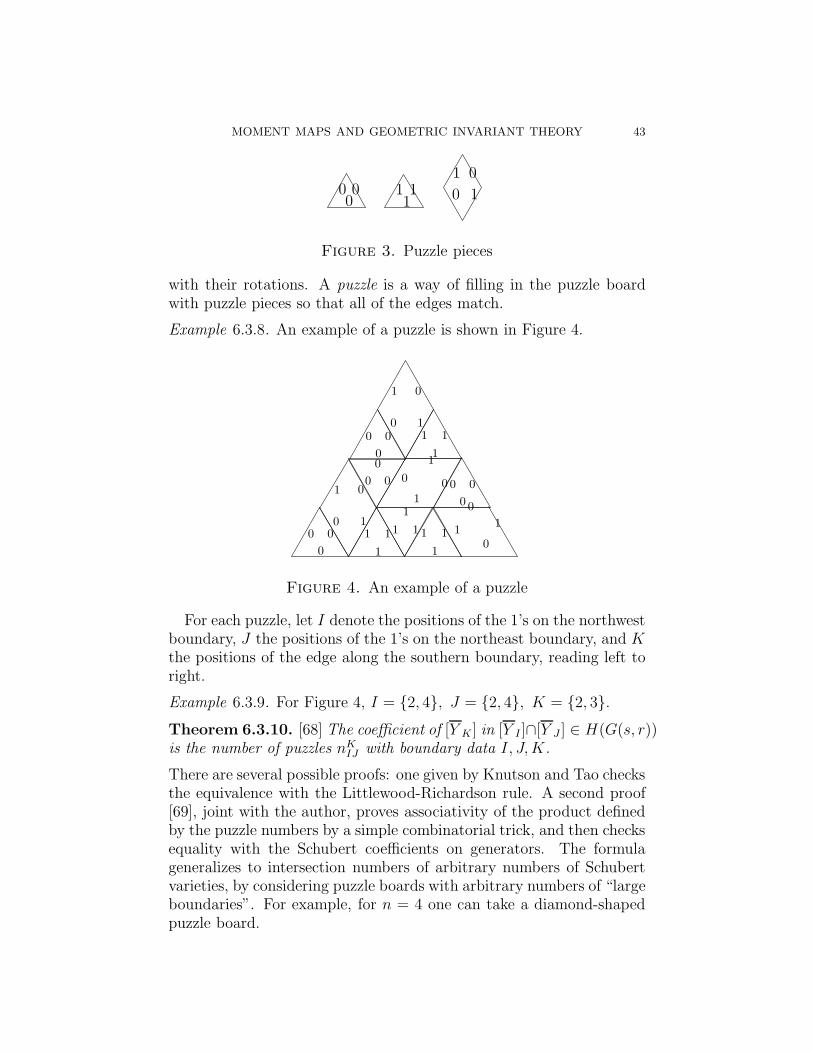
MOMENT MAPS AND GEOMETRIC INVARIANT THEORY 43
000
11 1
1 0
0 1
Figure 3. Puzzle pieces
with their rotations. A puzzle is a way of filling in the puzzle boardwith puzzle pieces so that all of the edges match.
Example 6.3.8. An example of a puzzle is shown in Figure 4.
1 0
0 1
0
0
0
0
0
0
1
1 10
0
0
0
0
01 0
0 1 1
0
0
1
1
00
1
1
1 1
1
1 1
1
1 1
Figure 4. An example of a puzzle
For each puzzle, let I denote the positions of the 1’s on the northwestboundary, J the positions of the 1’s on the northeast boundary, and Kthe positions of the edge along the southern boundary, reading left toright.
Example 6.3.9. For Figure 4, I = 2, 4, J = 2, 4, K = 2, 3.
Theorem 6.3.10. [68] The coefficient of [Y K ] in [Y I ]∩[Y J ] ∈ H(G(s, r))is the number of puzzles nK
IJ with boundary data I, J,K.
There are several possible proofs: one given by Knutson and Tao checksthe equivalence with the Littlewood-Richardson rule. A second proof[69], joint with the author, proves associativity of the product definedby the puzzle numbers by a simple combinatorial trick, and then checksequality with the Schubert coefficients on generators. The formulageneralizes to intersection numbers of arbitrary numbers of Schubertvarieties, by considering puzzle boards with arbitrary numbers of “largeboundaries”. For example, for n = 4 one can take a diamond-shapedpuzzle board.

44 CHRIS WOODWARD, RUTGERS UNIVERSITY, NEW BRUNSWICK
Combining this combinatorial description with Klyachko’s argumentgives the following:
Corollary 6.3.11. If there is a puzzle whose 1’s on the boundary arein positions I, J,K then the inequality
∑
i∈I
λi(H1) +∑
j∈J
λj(H2) ≤∑
k∈K
λk(H1 +H2)
holds for any Hermitian matrices A,B, and these inequalities togetherwith the trace equality
n∑
i=1
λi(H1) +
n∑
j=1
λj(H2) =
n∑
k=1
λk(H1 +H2)
give sufficient conditions for a triple (λ(H1), λ(H2), λ(H1 + H2)) tooccur.
Example 6.3.12. The puzzle in Example 6.3.8 gives the inequality λ2(H1)+λ4(H1) + λ2(H2) + λ4(H2) ≤ λ2(H1 +H2) + λ3(H1 +H2).
The following theorem of Knutson, Tao, and the author [68] (see alsothe review [67]), extending previous work of Belkale [12], describes aminimal set of inequalities:
Theorem 6.3.13. The inequalities corresponding to I, J,K with nKIJ =
1 together with the trace equality form a complete and irredundant setof necessary and sufficient conditions for the Horn problem for the sumof two Hermitian matrices.
Many other problems of this type can be solved in the same way; forexample see Agnihotri-Woodward [2] for a discussion of the possibleeigenvalues of a product of unitary matrices, and relations with theinvariant theory of quantum groups. In this case the existence of agood combinatorial model computing the eigenvalue inequalities is stillopen.
7. The stratifications of Hesselink, Kirwan, and Ness
According to work of Kirwan [61] and Ness [84], the semistable lo-cus of a G-variety X ⊂ P(V ) can be considered the open stratum in aMorse-type stratification ofX . A theorem of Ness describes the equiva-lence of this stratification with one introduced by Hesselink [52], whichmeasures the slope of instability of a point by its maximal Hilbert-Mumford weight.

MOMENT MAPS AND GEOMETRIC INVARIANT THEORY 45
7.1. The Kirwan-Ness stratification. Let X be a Hamiltonian K-manifold with proper moment map Φ : X → k∨. Let ( , ) : k → k → R
be an invariant metric on k inducing an identification k → k∨. Let
φ =1
2(Φ,Φ) : X → R
denote the norm-square of the moment map. The notation Φ(x)X ∈Vect(X) denotes the vector field determined by Φ(x), and Φ(x)X(x) ∈TxX its evaluation at x.
Lemma 7.1.1. crit(φ) = x ∈ X,Φ(x)X(x) = 0.
Proof. We have dφ(x) = (Φ(x), dΦ(x)) = −ιΦ(x)X (x)ωx. Since ω is non-degenerate, dφ(x) vanishes iff Φ(x)X(x) ∈ TxX does.
Example 7.1.2. LetX = P2 andK = U(1)2 acting by (g1, g2)[z0, z1, z2] =[z0, g
−11 z1, g
−12 z2]. Consider the moment map
Φ([z0, z1, z2]) 7→ (|z1|2/2, |z2|
2/2)− (1/4, 1/4),
which has image the convex hull
∆(X) = hull(−1/4,−1/4), (−1/4, 3/4), (3/4,−1/4).
The critical sets are the level sets of Φ at (0, 0), (−1/4, 0), (0,−1/4), (1/4, 1/4),(−1/4,−1/4), (−1/4, 3/4), (3/4,−1/4), see Figure 5.
Figure 5. Critical values for X = P2
Lemma 7.1.3. Φ(crit(φ)) is a discrete union of K-orbits in k∨, calledthe set of types for X.
Proof. Suppose first that K is abelian. Consider the orbit-type decom-position
X =⋃
H⊂K
XH , XH = x ∈ X|Kx = H.
where the union is over subgroups H ⊂ K. It follows from standardslice theorems that each XH is a smooth manifold. Let h denote the Lie

46 CHRIS WOODWARD, RUTGERS UNIVERSITY, NEW BRUNSWICK
algebra of H . By Lemma 3.3.2, Φ(XH) is an open subset of an affinesubspace parallel to ann(h). Thus Φ(XH ∩ crit(φ)) = λ ∈ Φ(XH)|λ ∈h which is the set containing the unique point in Φ(XH) closest to0, if it exists, and empty, otherwise. Since Φ is proper, the pre-imageof any compact set under Φ contains only finitely many orbit-types,which proves the theorem in the abelian case.Suppose that K is possibly non-abelian with maximal torus T . The
action of T onX is also Hamiltonian with moment map ΦT obtained bycomposing Φ with the projection of k∨ onto t∨. Let φT = (ΦT ,ΦT )/2.Since φ is K-invariant, any critical point is conjugate to a point x ∈crit(φ) with Φ(x) ∈ t∨. Then x ∈ crit(φ) iff x ∈ crit(φT ) iff Φ(x) is atype for the action of T . Hence the types for K are locally finite.
Choose a compatible K-invariant metric on X , and let grad(φ) ∈Vect(X) denote the gradient of φ.
Lemma 7.1.4. The gradient of φ is grad(φ)(x) = J(x)Φ(x)X(x).
Proof. Using the proof of Lemma 7.1.1, for v ∈ TxX
gx(grad(φ)(x), v) = Dxφ(v) = −ωx(Φ(x)X(x), v) = gx(J(x)Φ(x)X(x), v).
The claim follows.
Let ϕt : X → X be the flow of − grad(φ); since Φ is proper, so is φand so ϕt exists for all times t ∈ [0,∞).
Proposition 7.1.5 (Duistermaat, see [74], [113]). Any trajectory of ϕt
has a limit.
For the construction of the Kirwan stratification the actual conver-gence of ϕt is not needed. For each type λ, let Cλ = Φ−1(Kλ)∩ crit(φ)denote the corresponding component of the critical set of φ. Since theset of types is discrete, any two limit points are contained in someCλ ⊂ crit(φ), and in fact in the same connected component of crit(φ).Let Xλ denote the set of points x ∈ X flowing to Cλ,
Xλ := ϕt(x), t ∈ [0,∞) ∩ Cλ 6= ∅..
Note that since φ is not Morse-Bott in general, there is no guaranteethatXλ is smooth. The Kirwan-Ness stratification is the decomposition[61], [84]:
X =⋃
λ
Xλ.

MOMENT MAPS AND GEOMETRIC INVARIANT THEORY 47
Theorem 7.1.6 (Kirwan). There exists an invariant metric on X sothat each stratum Xλ is smooth. The spectral sequence for the equivari-ant stratification X = ∪λXλ collapses at the second page, so that
HK(X) ∼=⊕
λ
HK(Xλ).
In particular the canonical map HK(X) → HK(Φ−1(0)) (which is iso-
morphic to H(X//K) if K acts freely on Φ−1(0)) is a surjection andthe equivariant Poincare polynomial of X
pKX(t) =∑
tj rankHjK(X)
is given by
pkX(t) =∑
λ
(−1)codim(Xλ)pKXλ(t).
IfX acts freely on Φ−1(0) this means that the difference pKX(t)−pX//K(t)is a finite sum of contributions from fixed point sets of one-parametersubgroups. We will see a version of this formula for sheaf cohomologyin the last chapter.In the case that X is a Kahler Hamiltonian K-manifold with proper
moment map, the Kirwan-Ness stratification has a more explicit de-scription. For each type λ let ϕλ,t denote the time t flow of− grad〈Φ, λ〉,Zλ the component of the fixed point set Xλ of the action of λ contain-ing Cλ, Yλ the subset of X flowing to Zλ under ϕλ,t, Kλ the centralizerof λ, and U(1)λ the one-parameter subgroup generated by λ. ThenKλ/U(1)λ acts naturally on Zλ in Hamiltonian fashion with momentmap denoted Φλ, obtained by restricting Φ to Zλ and projecting outthe direction generated by λ. We denote by Zss
λ the set of points flow-ing to Φ−1
λ (0) under the flow of minus the gradient of the norm-squareof Φλ. Let Y
ssλ denote the inverse image of Zss
λ in Yλ.
Theorem 7.1.7 (Kirwan [61]). Let X be a compact Kahler Hamilton-ian K-manifold with proper moment map Φ : X → k∨. For the Kahlermetric each Xλ is a G-invariant complex submanifold, each Yλ is a Pλ-invariant complex submanifold, and G×Pλ
Y ssλ → Xλ, [g, y] 7→ gy is an
isomorphism of complex G-manifolds.
We give a proof, and explain the relation with a theorem of Ness[84], in the following section. In the point of view we will present, akey fact is that the gradient flow of the norm-square of the momentmap is essentially equivalent to the gradient flow of the Kempf-Nessfunction, as was pointed out in Donaldson-Kronheimer [30, Section 6].Let X be a Kahler Hamiltonian K-manifold with proper moment map.For any x ∈ X , let xt denote the trajectory of the gradient flow of −φ

48 CHRIS WOODWARD, RUTGERS UNIVERSITY, NEW BRUNSWICK
starting at x. On the other hand, let ψ : K\G → R be the Kempf-Ness function for x. We may also consider the gradient flow of ψ, withrespect to the given metric on k.
Proposition 7.1.8. Let X, x, ψ be as above. The map
K\G→ X/K, [g] 7→ [gx]
maps the gradient trajectories of ψ onto the image of the gradient tra-jectories of φ mod K.
Proof. Using Corollary 5.2.3,
JX((grad(ψ))([g]))X(gx) = JX(Φ(gx))X(gx)
= (grad(φ))(gx).
The vector field on G given by g 7→ i grad(ψ)([g]) has trajectories thatmap to the gradient trajectories of grad(ψ) under G → K\G, and tothe trajectories of grad(φ) under G→ X , which gives the result.
In particular, since the trajectories of ψ exist for all time by the boundon Φ, any trajectory of − grad(φ) is contained in a single G-orbit:xt ∈ Gx, ∀x ∈ X, t ∈ R.
Corollary 7.1.9. ψ is bounded from below iff the gradient flow for −φconverges to Φ−1(0).
Proof. In the algebraic case, this is nothing but a reformulation of 4.3.4.For the Kahler case, note that if ψ is bounded from below then grad(ψ)converges to zero along any gradient trajectory, and by equivalenceof gradient flows 7.1.8 it follows that Φ must converge to zero. Theconverse follows as in the proof of Theorem 5.5.9, using that grad(ψ)converges to zero exponentially fast along any one-parameter subgroupwhose limit corresponds to a polystable point.
One obtains an analytic proof of the Hilbert-Mumford criterion The-orem 4.3.1 by combining Corollary 7.1.9 and Theorem 5.4.2.
Remark 7.1.10. A rather confusing point is that if ψ : K\G → R
is a Kempf-Ness function, then the slope function (K\G)∞ → R ofTheorem 5.4.2 is not continuous in the topology on (K\G)∞ inducedby the identification with the unit sphere in the Lie algebra k, but ratheronly in the topology induced by the Tits metric. This happens alreadyfor the action of SL(2,C) on P1: the asymptotic slope for the Kempf-Ness function for [0, 1] is 1 for every direction except that generated bydiag(i,−i), where it is −1; the topology induced by the Tits metric inthis case is discrete.

MOMENT MAPS AND GEOMETRIC INVARIANT THEORY 49
7.2. The Hesselink stratification. LetX ⊂ P(V ) be a projective G-variety, or more generally a compact Kahler Hamiltonian K-manifold.The Hesselink stratification uses the weights appearing in the Hilbert-Mumford criterion to construct a stratification on X : Define for anynon-zero λ ∈ k the Hilbert-Mumford slope
µλ(x) = 〈Φ(xλ), λ〉/‖λ‖.
By Corollary 5.2.3, the Hilbert-Mumford slope is equal to the asymp-totic slope of the Kempf-Ness function studied in Theorem 5.4.2.
Definition 7.2.1. A point x ∈ X is
(a) slope semistable iff µλ(x) ≤ 0 for all λ,(b) slope stable iff µλ(x) < 0 for all λ,(c) slope unstable iff x is not semistable, and(d) slope polystable iff it is slope semistable and µλ(x) = 0 implies
µ−λ(x) = 0 for all λ.
Slope semistability might also be called Hilbert-Mumford semista-bility, but this seems a little unwieldy. We have already seen in theproof of the Kempf-Ness theorem that slope semistability is equivalentto semistability. The equivalence of slope polystability with polysta-bility is proved in Mundet [56]. It follows from Section 5.5 that a pointx ∈ X is polystable but not stable iff its Jordan-Holder cone containsa line.The set of destabilizing one-parameter subgroups is studied by Hes-
selink in the algebraic case [52], [53], see also Ramanan-Ramanathan[90]. For any λ we denote by Gλ the centralizer of λ and by C∗
λ the one-parameter subgroup generated by λ. Obviously C∗
λ ⊂ Gλ. Let x ∈ Xand Zλ denote the component of Xλ containing xλ. Then the actionof Gλ on Zλ descends to an action of Gλ/C
∗λ. Furthermore, the inner
product on k determines a splitting gλ = Cλ⊕ gλ/Cλ which defines alift of Gλ/C
∗λ to the polarizing line bundle, at least up to finite cover.
So we may consider Zλ as a polarized Gλ/C∗λ-variety, with the caveat
that the polarization depends on the choice of inner product on k.
Theorem 7.2.2. Any unstable x has a unique (up to scalar multiple)maximally destabilizing one-parameter subgroup generated by λ ∈ k
with the property that xλ is a semistable point for the action of Gλ/C∗λ
on Zλ and λ is maximally destabilizing: µν(x) ≤ µλ(x) for all ν ∈k− 0 and equality holds iff R+ν = R+λ.
Proof. We already proved in Theorem 5.4.2 the existence of a maxi-mally destabilizing one-parameter subgroup generated by some λ ∈ k.It remains to show that for any x ∈ X , xλ is semistable for Gλ/C
∗λ,

50 CHRIS WOODWARD, RUTGERS UNIVERSITY, NEW BRUNSWICK
or what is equivalent, Φ((xλ)t) converges to Kλ. Since (Φ(xλ), λ) =(λ, λ), the function ψ goes to −∞ along exp(−iλt)x as fast as xt. Iflim ‖Φ((xλ)t)‖ > λ, then ψ((exp(−iλt1)x)t2) as t1 ≫ t2 → ∞ goes to−∞ faster than ψ(xt), which contradicts convexity of ψ as in the proofof Theorem 5.4.2. Hence ‖Φ((xλ)t)‖ → λ. Now the gradient trajec-tories for exp(−iλt)x converge to a broken gradient trajectory for xλ;since each piece in the broken gradient trajectory must decrease φ, thelimit has only one piece. That is, Φ((xλ)t) → Kλ.
Let Λ denote the set of equivalence classes of one-parameter sub-groups appearing in Hesselink’s theorem (with equivalence given bythe adjoint action) we call the decomposition X = ∪λXλ the Hesselinkstratification of X .
Remark 7.2.3. The Hesselink stratification is the finite-dimensionalanalog of the Shatz stratification [97] of the moduli stack of vectorbundles on a curve by the type of the Harder-Narasimhan filtration.
The following is proved in the algebraic case by Ness [84].
Theorem 7.2.4. The Hesselink and Kirwan-Ness stratifications agree.
Proof. By Theorem 5.4.2 part (c).
Proof of Kirwan’s theorem 7.1.7. Let ψ = ψv be a Kempf-Ness func-tion, and Xλ a Hesselink stratum (or equivalently, a Kirwan-Ness stra-tum.) Let Uλ denote the set of points in x with direction of maximallynegative slope λ. Uniqueness of λ implies that if x ∈ Uλ and g ∈ Gis such that gx ∈ Uλ, then g ∈ Pλ. Indeed, note G = KPλ and Uλ isPλ-stable. Hence it suffices to consider the case g ∈ K, and then gλis also a direction of maximal descent. Hence gλ = λ which impliesthat g ∈ Kλ, hence g ∈ Pλ. This implies Xλ = G ×Pλ
Uλ. To seethat Uλ = Y ss
λ of Section 7.1, note that Uλ ⊂ Y ssλ by Theorem 7.2.2.
On the other hand, Y ssλ is contained in Uλ: any point in Y ss
λ has apoint in Φ−1(λ) in its orbit-closure, and ‖λ‖2 minimizes ‖Φ‖2 on Y ss
λ
which implies that λ is the direction of maximally negative slope. Thiscompletes the proof.
Remark 7.2.5. Suppose ω ∈ Ω2(X) is a closed two form that is notsymplectic, but satisfies ω(ξX, JξX) > 0 for any ξ ∈ k. The proofabove works equally well for moment maps associated to such two-forms. That is, only non-degeneracy of the two-form on the directionsgenerated by the action is used in the proof.

MOMENT MAPS AND GEOMETRIC INVARIANT THEORY 51
8. Moment polytopes
According to work of Atiyah, Guillemin-Sternberg, and Kirwan, thequotient of the image of the moment map is convex. (This sectioncould have been placed before that on Schur-Horn convexity.)
8.1. Convexity theorems for Hamiltonian actions. Let X be aHamiltonian K-manifold with moment map Φ. The moment image ofX is Φ(X) ⊂ k. The quotient
∆(X) := Φ(X)/K ⊂ k∨/K
can be identified with a subset of the convex cone t∨+∼= k∨/K.
Example 8.1.1. If X = Pn−1 and G = U(1)n acts by the standardrepresentation, then the moment image is the standard n-simplex
Φ(X) = (ν1, . . . , νn) ∈ Rn≥0 | ν1 + . . .+ νn = 1,
see (3). The coordinate hyperplane zj = 0 ⊂ X maps to the j-thfacet νj = 0 ⊂ Φ(X).
Another description of the moment polytope ∆(X) involves the shiftedsymplectic quotients: for λ ∈ k∨, the quotient
X//λK := Φ−1(Kλ)/K = (O−λ ×X)//K
is the symplectic quotient of X at λ. The shifted symplectic quotientis the classical analog of the multiplicity space HomK(Vλ, V ) of a rep-resentation V in the following sense:
Proposition 8.1.2. Let X be a polarized projective G-variety and λa dominant weight. Then R(X//λG)d = HomG(Vdλ, R(X)d) for anyd ≥ 0.
Proof. Combining the Borel-Weil and Kempf-Ness theorems gives
R(X//λK)d = R(Kλ− ×X)Kd
= (V ∨dλ ⊗ R(X)d)
K
= HomK(Vdλ, R(X)d)
The following is immediate from the definitions:
Lemma 8.1.3. ∆(X) = λ | X//λK 6= ∅ is the set of λ for which theshifted symplectic quotient X//λK is non-empty.
The set ∆(X) is the “classical analog” of the set of simple modulesappearing in a G-module. Let ∆Q(X) := Λ∨
Q ∩∆(X) denote the set ofrational points in ∆(X); furthermore ∆Q(X) is dense in ∆(X), see forexample [73].

52 CHRIS WOODWARD, RUTGERS UNIVERSITY, NEW BRUNSWICK
Theorem 8.1.4. ∆Q(X) = ∆(X)∩Λ∨Q is equal to the set of points λ/d
such that Vλ ⊂ R(X)d.
Proof. By Lemma 8.1.3 and Proposition 8.1.2.
Recall that a convex polyhedron is the intersection of a finite numberof half spaces, while a convex polytope is the convex hull of a finitenumber of points. The fundamental theorem of convex geometry saysthat any compact convex polyhedron is a convex polytope and vice-versa.
Theorem 8.1.5 (Atiyah [7], Guillemin-Sternberg [37] for the abeliancase, Kirwan [62] for the non-abelian case). Let K be a compact, con-nected Lie group and X a compact connected Hamiltonian K-manifold.Then ∆(X) is a convex polytope. If K is abelian, then ∆(X) is the con-vex hull of the image Φ(XK) of the fixed point set XK of K.
∆(X) is the moment polytope of X . The arguments of Atiyah andGuillemin-Sternberg in [7], [37] are Morse-theoretic. The equivariantversion of Darboux’s theorem implies that the functions 〈Φ, ξ〉 haveonly critical sets of even index, and this implies that the level sets〈Φ, ξ〉−1(c) are connected. Using an inductive procedure one showsthat for any subtorus K1 ⊂ K, the level sets of the moment map forΦ1 are connected as well. Taking K1 of codimension one, this showsthat the intersection of Φ(X) with any rational line is connected andit follows that Φ(X) is convex. The reader is referred to the originalpapers for details. Kirwan’s non-abelian version uses the Morse the-ory of the norm-square of the moment map. See Lerman-Meinrenken-Tolman-Woodward [73] for a derivation of non-abelian convexity fromthe abelian case.Brion [18], following earlier work of Mumford [84, Appendix], pointed
out the following proof of convexity, which in language of geometricquantization would be called a “quantum” proof: Suppose λj/dj ∈∆Q(X), j = 0, 1. Let vj ∈ R(X)dj be corresponding highest weightvectors. Then for any n0, n1 ∈ N, vn0
0 vn11 ∈ R(X)n0d0+n1d1 is a highest
weight vector, so
n0λ0 + n1λ1n0d0 + n1d1
=d0n0
d0n0 + d1n1(λ0/d0) +
d1n1
n0d0 + n1d1(λ1/d1) ∈ ∆Q(X).
This implies that ∆Q(X) is convex.The inequalities of the previous section (for example, the Horn-
Klyachko problem) can now be seen as the inequalities describing themoment polytopes of products of coadjoint orbits.

MOMENT MAPS AND GEOMETRIC INVARIANT THEORY 53
8.2. Convexity theorems for orbit-closures. In the case that Xis Kahler, Atiyah [7] also described the images of orbit-closures underthe moment map, in the case that K is abelian. Of course if theorbit-closure is smooth, then this falls under the assumptions of theprevious convexity theorem, but Atiyah’s theorem also includes thecase of singular orbit-closures:
Theorem 8.2.1. [9, Theorem 2] Let K be a torus, G its complexifi-cation, and X a Kahler Hamiltonian K-manifold. Let Y ⊂ X be aG-orbit. Then
(a) ∆ := Φ(Y ) is a convex polytope with vertices Φ(Y ∩XG);(b) For each open face F ⊂ ∆, Φ−1(F ) ∩ Y is a single G-orbit.(c) Φ induces a homeomorphism of Y /G onto ∆.
We will describe Atiyah’s arguments since they are brief and areclosely related to the one-parameter subgroups of Hesselink as well asthe Jordan-Holder subgroups of Section 5.5.9. The proof depends onthe following
Lemma 8.2.2. Let Y ⊂ X be a G-orbit and y ∈ Y . Then
(a) yλ = limt→∞(exp(itλ)y) exists and lies in the fixed point set Xλ;(b) limt→∞〈Φ(exp(itλ)y), λ〉 exists and is a constant dλ independent
of y.(c) dλ = supy∈Y 〈Φ(y), λ〉 is the asymptotic slope in Theorem 5.4.2.
Suppose that λ is generic so that XG = Xλ. The Lemma implies
supy∈Y
〈Φ(y), λ〉 = supy∈XG∩Y
〈Φ(y), λ〉.
Hence Φ(Y ) is contained in the convex hull of Φ(XG ∩ Y ). To see thatΦ(Y ) = ∆, Atiyah notes that for any y ∈ Y and direction ξ ∈ k of unitlength, there exists a time t(ξ) such that
〈Φ(exp(it(ξ)ξy), ξ〉 =1
2(Φ(y) + d(ξ)).
The set of points exp(iξ)y with ‖ξ‖ ≤ t(ξ/‖ξ‖) defines a neighborhoodU of y in Y with Φ(U) = Φ(y)+ 1
2(∆−Φ(y)); this immediately implies
that Φ(Y ) is both open and closed in ∆ and hence equal to ∆.To prove the third part of the Theorem, Atiyah considers for any
λ ∈ k and fixed point component Z ⊂ Xλ, the unstable manifold Zu
consisting of all points that flow to Z under exp(itλ). By the stablemanifold theorem Zu is a smooth manifold and the limit of the flowdefines a smooth G-equivariant projection Zu → Z. In particular, ifZ is any component of Xλ containing a limit point of Y then Y ⊂ Zu

54 CHRIS WOODWARD, RUTGERS UNIVERSITY, NEW BRUNSWICK
and Y ∩ Z is a single G-orbit. From this it follows that Φ(Z ∩ Y ) is aface of ∆ with fibers the orbits of the compact torus K, see [9, p. 10],and this completes the proof.
Remark 8.2.3. Atiyah’s theorem makes the theory of polystable pointsand Jordan-Holder vector described in Section 5.5 substantially easierin the abelian case. One sees that the “Jordan-Holder” cone of Theorem5.5.9 is the dual cone to the face of the polytope containing 0, in thecase that Y is a semistable orbit.
Atiyah’s convexity theorem for orbit-closures has been generalizedto Borel subgroups by Guillemin and Sjamaar [44].
9. Multiplicity-free actions
In certain cases Hamiltonian or algebraic actions may be classifiedby combinatorial data related to the moment map. In this sectionwe discuss an example of this, the multiplicity-free case, in which thesymplectic and git quotients are points.
9.1. Toric varieties and Delzant’s theorem. A toric variety is anirreducible normal G-variety X such that G is an algebraic torus and Xcontains an open G-orbit. Affine toric varieties are naturally classifiedby monoidsM in the group Λ∨ of weights of G, with the correspondingtoric variety given by Spec(C[M ]). Each such monoid spans a rationalcone in Λ∨
Q, and defines a dual cone in ΛQ. Toric varieties with trivialgeneric stabilizer are classified by fans in ΛQ, that is, collections ofcones such that any intersection of a cone is again a cone in the fan,see Oda [87] or Fulton [34].
Example 9.1.1. Suppose thatX = P2 with action given by (w1, w2)[z0, z1, z2] =[z0, w
−11 z1, w
−12 z2]. There are seven orbits, given by non-vanishing of
various coordinates, and in particular, three closed orbits [1, 0, 0], [0, 1, 0], [0, 0, 1],whose cones are generated by pairs of vectors (1, 1), (−1, 0), (1, 1), (0,−1),and (0,−1), (0,−1). The fan contains these three cones, and their inter-sections; this is the dual fan to the moment polytope hull((0, 0), (1, 0), (0, 1)).
A Hamiltonian torus action is multiplicity free or completely inte-grable if all the symplectic quotients are points, or equivalently, eachfiber of the moment map is an orbit of the torus.
Example 9.1.2. The U(1)n action on Pn is multiplicity-free, since thefibers of the moment map are given by [z0, . . . , zn] with |z1|, . . . |zn|fixed, which are orbits of U(1)n.
Multiplicity-free Hamiltonian torus actions are classified by a theoremof Delzant.

MOMENT MAPS AND GEOMETRIC INVARIANT THEORY 55
Definition 9.1.3. A polytope ∆ ⊂ k∨ is called Delzant if the normalcone at any vertex is generated by a basis of the weight lattice Λ∨ ⊂ k∨.
Theorem 9.1.4 (Delzant [28]). There exists a one-to-one correspon-dence between Delzant polytopes and multiplicity-free torus actions oncompact connected manifolds with trivial stabilizer, given by X 7→Φ(X). Any compact connected multiplicity-free Hamiltonian torus ac-tion has the structure of a smooth projective toric variety.
Note that any compatible complex structure is unique up to isomor-phism, but not up to Kahler isomorphism. That is, any toric varietyhas many non-equivalent Kahler structures, see Guillemin [43].There are “local” and “local-to-global” parts of the proof; the local
part follows from the equivariant Darboux theorem, while the “local-to-global” part uses the vanishing of a certain sheaf cohomology groupover the polytope.Existence of a smooth projective toric variety with a given polytope
follows from, for example, Lerman’s method of symplectic cutting [72]which we now describe. We begin with the simplest case, when X is aHamiltonian S1-manifold with moment map Φ : X → R. The diagonalS1-action on X × C is Hamiltonian with moment map
ΦX×C : (x, z) 7→ Φ(x)− |z|2/2.
Its symplectic quotient at any value λ
X≥λ := (X × C)//λS1
is called the symplectic cut of X at λ admits a decomposition
(X × C)//λS1 ∼= X//λS
1 ∪ (X × C∗)//λS1 ∼= X//λS
1 ∪ Φ−1((λ,∞)).
It follows from the definitions that the inclusion of Φ−1((λ,∞)) in X≥λ
is symplectic and so X≥λ is obtained by removing Φ−1((−∞, λ)) and“closing off” the boundary by quotienting it by S1.More generally, suppose that K is a torus, ξ ∈ k any rational vector,
and λ ∈ R. Let U(1)λ denote the one-parameter subgroup generatedby λ, with moment map 〈Φ, λ〉. Then the symplectic cut X≥λ = (X ×C)//λU(1)λ ∼= X//λU(1)λ ∪ 〈Φ, v〉 > λ admits the structure of aHamiltonian K-manifold with moment polytope Φ(X≥λ) = Φ(X) ∩〈ν, v〉 ≥ λ.
Example 9.1.5. Let X = P2 equipped with U(1)2-action given by withweights (0, 0), (−2, 0), (0,−2). The moment polytope is then the convexhull of (0, 0), (2, 0), (0, 2). Let λ = (0,−1) so that the one-parametersubgroup generated by λ acts with moment map
[z0, z1, z2] 7→ −2|z1|2/(|z0|
2 + |z1|2 + |z2|
2).

56 CHRIS WOODWARD, RUTGERS UNIVERSITY, NEW BRUNSWICK
The symplectic cut at −1 is then a toric variety with polytope theconvex hull of (0, 0), (0, 2), (1, 0), (1, 1), see Figure 6.
Figure 6. Effect of cutting on a moment polytope
Suppose that ∆ is a Delzant polytope defined by inequalities
∆ = ν ∈ k∨ | 〈ν, vj〉 ≥ λj, j = 1, . . . , m
for some vectors vj ∈ k and some constants λj ∈ R, j = 1, . . . , m. LetX = T∨K, with moment image k∨ and the standard Kahler structure.Performing a symplectic cut for each inequality gives a Kahler manifoldwith Hamiltonian K action and moment polytope ∆.Alternatively any smooth projective toric variety is a symplectic or
geometric invariant theory quotient of affine space X = Cm. There isan explicit description of the semistable locus given by Audin [10] andCox [27].
9.2. Multiplicity-free actions and spherical varieties. LetK be acompact connected Lie group. Recall that aK-module V ismultiplicity-free iff HomK(Vλ, V ) is dimension at most one, for any simpleK-moduleVλ iff EndK(V ) is abelian, using Schur’s lemma. The definition in part(a) of the following was introduced in Guillemin-Sternberg [45]:
Theorem 9.2.1. (see [111, Appendix]) The following conditions areequivalent, and if they hold the action is multiplicity-free:
(a) C∞(X)K is an abelian Poisson algebra.(b) The symplectic quotient X//λK := Φ−1(Kλ)/K is a point for
all λ.
Proof. We denote by rλ : C∞(X)K → C∞(X//λK) the map of Poissonalgebras induced by the symplectic quotient construction, if λ is free.In general, we define C∞(X//λK) := C∞(X)K/f, f |Φ−1(λ) = 0. Alemma of Arms, Cushman, and Gotay [6], see Sjamaar-Lerman [100],says that this quotient is a non-degenerate Poisson algebra, that is,the bracket vanishes only on constant functions. Suppose (a). Sincerλ is surjective, C∞(X//λK) is abelian as well, and so X//λK mustbe discrete, hence a point by Kirwan’s results. Conversely, if all the

MOMENT MAPS AND GEOMETRIC INVARIANT THEORY 57
reduced spaces are points and f, g ∈ C∞(X)K then rλ(f, g) = 0 forall λ implies that f, g = 0.
The complex analogs of multiplicity-free Hamiltonian actions arecalled spherical varieties. Let G be a connected complex reductivegroup. For the following, see Brion-Luna-Vust [20], the review [65], orthe second part of Brion’s review in this volume.
Theorem 9.2.2. The following conditions for a normal G-variety Xare equivalent; if they hold X is called spherical:
(a) some (hence any) Borel subgroup B has an open orbit;(b) the space of rational functions C(X) is a multiplicity-free G-
module;(c) some (hence any) Borel subgroup B has finitely many orbits.
Remark 9.2.3. For an arbitrary group action, existence of a dense orbitdoes not imply finitely many orbits. For example, consider the action ofSL(n,C) on the space of n×n matrices on the left: any two invertiblematrices are related by an element of SL(n,C), but there are infinitelymany orbits of degenerate matrices distinguished by their kernels.
The classification of toric varieties is generalized to spherical varietiesas a special case of a theorem of Luna-Vust [77] which gives a classifica-tion of spherical varieties by their generic isotropy group and a coloredfan, see the contribution of Pezzini in this volume or Knop [65]. Eachcolored fan is a collection of colored cones, convex cones in the space ΛX
dual to the space Λ∨X of characters corresponding to B-semiinvariant
functions C(X)(B), together with a finite set of B-stable divisors, sat-isfying certain conditions. The classification of generic isotropy groupsthat appear, which are called spherical subgroups, is the subject of anopen conjecture of Luna, see the contribution of Bravi in this volume.The relation between multiplicity-free Hamiltonian actions and spher-ical varieties is given by the following, which is a consequence of theKempf-Ness theorem:
Proposition 9.2.4. A smooth G-variety X ⊂ P(V ) is spherical if andonly if it is a multiplicity-free Hamiltonian K-manifold.
Proof. By Proposition 8.1.2 X//λK = pt iff HomG(Vλ, H0(X,OX(d)))
is dimension one or zero for all d ≥ 0. This holds for all λ and d ≥ 0 iffC(X)d is a multiplicity-free G-module for all d ≥ 0 iff X is spherical.
In contrast to the toric case, not every multiplicity-free Hamiltonianaction admits the structure of a spherical variety [112].

58 CHRIS WOODWARD, RUTGERS UNIVERSITY, NEW BRUNSWICK
9.3. Moment polytopes of spherical varieties. We have alreadyseen several examples of the following:
Theorem 9.3.1. Let X be a smooth polarized spherical K-variety withmoment polytope ∆ and trivial generic stabilizer. Then H0(X,OX(1))is the multiplicity-free K-module whose weights are the integral points∆ ∩ k∨ of ∆.
Proof. By Proposition 8.1.2 and the fact that the symplectic quotientsare points.
The moment polytope of a spherical variety X is described by a finiteset of linear inequalities corresponding to the B-stable divisors of Xwhich was described by Brion [19] in the non-abelian case. Let X bea spherical G-variety and L → X a G-equivariant line bundle. Firstsome notation: Let C(X) denote the space of rational functions onX , and C(X)(B) the space of B-semiinvariant vectors. Let Λ∨
X ⊂ Λ∨
denote the group of weights appearing in C(X)(B). Let D(X) denotethe set of prime B-stable divisors of X . Each D ∈ D(X) defines avaluation C(X)(B) → Z and so a vector vD in the dual ΛX of Λ∨
X . LetC(X,L) denote the space of rational sections of L, and s ∈ C(X,L)(B)
with weight µ(s). Let nD(s) denote the order of vanishing of s atD. Consider the identification C(X)(B) → C(X,L)(B), f 7→ fs. Thesection fs is global iff fs vanishes to at least zeroth order on eachD ∈ D(X), iff f vanishes at least to order −nD. Thus
Proposition 9.3.2. Let X be a spherical G-variety, and L → X aG-line-bundle. The space of weights for elements of C(X,L)(B) is
∆(X,L) = µ ∈ Λ∨X |vD(µ) ≥ −nD(s)+ µ(s).
Example 9.3.3. Here is a typical application which appears in Brion[19] and seems to be due to Macdonald [78]:
Theorem 9.3.4. Let Vλ be a simple GL(r) module with highest weightλ = (λ1 ≥ . . . ≥ λr). Then Vλ ⊗ Sym(Cr) admits a multiplicity-free decomposition into simple modules Vµ with highest weights µ =(µ1, . . . , µr) satisfying
µ1 ≥ λ1 ≥ µ2 ≥ . . . µr ≥ λr.
Proof. We prove only the case r = 2; the general case is similar. Vλ ⊗Sym(C2) is isomorphic to the space of holomorphic sections of theline bundle π∗
1Lλ over X = P1 × C2 = ([w0, w1], (z0, z1), where π1 :P1 × C2 → P1 is projection on the first factor. We take B to bethe subgroup of upper-triangular invertible matrices. The B-invariantdivisors are given by a single G-invariant divisor D1 = (w, z)|z ∈ w

MOMENT MAPS AND GEOMETRIC INVARIANT THEORY 59
λ
Figure 7. Decomposition of Vλ ⊗ Sym(C2) via Brion’s method
and two B-stable divisors D2 = w = [1, 0] and D3 = z ∈ C ⊕ 0.The space of singular vectors C(X)(B) is generated by z1 − w1z0/w0
and z0 with highest weights (0, 1) resp. (1, 0). The B-stable divisorsare defined by D1 = z1/z0 = w1/w0, D2 = w1 = 0, D3 = z1 = 0respectively. Hence z1−w1z0/w0 vanishes to order 1 resp. −1, 0 on D1
resp. D2, D3; z1 vanishes to order 0 resp. 0, 1 on D1 resp. D2, D3. SovD1 = (0, 1), vD2 = (0,−1), vD3 = (1, 0). Taking s to be the section ofP1 with weight (λ1, λ2), which vanishes to order 0 on D1, λ1−λ2 in D2,and 0 on D3 one obtains nD1 = 0, nD2 = λ1 − λ2, nD3 = 0. This yieldsthe inequalities µ2 ≥ λ2, −µ2 ≥ −λ2 − (λ1 − λ2) = −λ1, µ1 ≥ λ1 asclaimed. See Figure 7.
Remark 9.3.5. Not every B-stable divisor defines a facet of the mo-ment polytope. This is already apparent in the case of the Borel-Weiltheorem, where for a group of rank r there are r B-stable divisors (theSchubert varieties of codimension one) but the moment polytope issimply a point.
Based on his work on the toric case, Delzant asked the question ofwhether compact multiplicity-free actions are classified by their mo-ment polytopes and generic stabilizers, and answered the question af-firmatively in the rank two case [29]. A result of Knop [64] reduces thisto the question of whether affine spherical varieties are classified bytheir moment polytopes and generic stabilizers of the compact groupactions; this conjecture has recently been proved by Losev [75], see alsohis review in this volume.In the torus case we have
Corollary 9.3.6. With X,K,OX(1) as above, if K is a torus then thedimension of H0(X,OX(1)) is the number of integral points ∆ ∩ k∨ of∆.

60 CHRIS WOODWARD, RUTGERS UNIVERSITY, NEW BRUNSWICK
The dimension of H0(X,OX(k)) can be computed by Riemann-Rochfor sufficiently large k, since OX(1) is by assumption positive. This ledto an interesting series of papers on formulas for the number of lat-tice points in a convex polytope which generalize the Euler-Maclaurinformula and were later proved combinatorially, see [21] for references.
10. Localization via sheaf cohomology
In this section we review various “fixed point methods” for com-puting moment polytopes, in the context of sheaf cohomology. Theseinclude not only the “localization” methods which take as input fixedpoint data for a one-parameter subgroup, but also the “non-abelianlocalization” principle which uses the Kirwan-Ness stratification.
10.1. Grothendieck’s local cohomology. A powerful technique forcomputing cohomology groups, and therefore for computing momentpolytopes, is Grothendieck’s local cohomology theory, exposed in [36]and Hartshorne [46]. Let X be a G-variety and Y ⊂ X a G-subvariety.Let E → X be a G-equivariant coherent sheaf. Denote by ΓY (X,E)the group of sections whose support is contained in Y . We denote byH i
Y the i-th derived functor of ΓY , so that the local cohomology groupH i
Y (X,E) is a G-module. These modules have the following properties:
Theorem 10.1.1. (a) (Long Exact Sequence) There is an exact tri-angle
. . .HY (X,E) → H(X,E) → H(X − Y,E|X − Y ) → . . .
(b) (Gysin isomorphism) Suppose Y ⊂ X is smooth. Then
HjY (X,E)
∼= Hj−codim(Y )(Y,E|Y ⊗ Eul(N)−1)
where N is the normal bundle of Y in X and Eul(N)−1 :=det(N)⊗Sym(N) (this is an inverse of the K-theory Euler classEul(N) = Λ(N∨) although we do not discuss K-theory here)
(c) (Spectral sequence associated to a stratification) Let X1 ⊂ X2 ⊂. . . ⊂ Xm = X be a filtration of X. There is a spectral sequence
m⊕
i=1
HXi−Xi−1(Xi, E|Xi) =⇒ H(X,E).
Let χ(X,E) =⊕
(−1)iH i(X,E) be the Euler characteristic, con-sidered as a virtual G-representation, and χY (X,E) the Euler charac-teristic of the local cohomology along Y . These will generally not befinite-dimensional, but rather in our cases of interest the multiplicityof each simple module is finite. Thus the formula below holds in the

MOMENT MAPS AND GEOMETRIC INVARIANT THEORY 61
completion of the representation ring, as an immediate consequence ofthe spectral sequence:
Corollary 10.1.2. Suppose that X1 ⊂ . . . ⊂ Xm = X is a filtration ofX such that the differences Xi −Xi−1 are smooth with normal bundlesNi → Xi −Xi−1. Then(13)
χ(X,E) =∑
i
(−1)codim(Xi−Xi−1)χ(Xi −Xi−1, E|Xi−Xi−1⊗ Eul(Ni)
−1)
if both sides are well-defined in the sense that the multiplicity of anysimple module is finite.
This formula applies to various filtrations associated to group actionsto give “localization” formulae.
Example 10.1.3. (Weyl character formula and Borel-Weil-Bott, c.f. Atiyah-Bott [8]) Let X = G/B− and E = OX(λ) so that if λ is dominantthen H0(X,E) = Vλ by Borel-Weil 6.1.1. The Bruhat decompositionX = ∪w∈WXw gives a filtration Xi = ∪w∈W,l(w)≥iXw. Each cell Xw
fibers over xw = wB/B with fiber Xw∼=Mw := b ∩ Ad(w)b. The nor-
mal bundle Xw has restriction to xw given by Nw = (b/b ∩Ad(w)b)∨.The formula (13) gives
χ(X,OX(λ)) =⊕
w∈W
(−1)l(w)χ(Xw, E|Xw ⊗ Sym(Nw)⊗ det(Nw))
=⊕
w∈W
(−1)l(w)χ(xw, E ⊗ Sym(Nw)⊗ det(Nw)⊗ Sym(M∨w )|xw)
=⊕
w∈W
(−1)l(w)Cwλ ⊗ Sym(b−)⊗ Cwρ−ρ
where ρ is the half-sum of positive roots. Thus its character is
(14)∑
w∈W
(−1)l(w) tw(λ+ρ)−ρ
∏
α>0(1− t−α).
Thus if λ is dominant then
Proposition 10.1.4. (Weyl character formula) The character of the ac-tion of T on Vλ is given by (14).
In general, suppose that w is such that w(λ+ρ)−ρ is dominant. Fromthe spectral sequence we see that the only contribution to χ(X,OX(λ))comes from H l(w)(X,OX(λ)), since l(w) = codim(Xw). This is a sim-ple G-module of highest weight w(λ + ρ) − ρ, since it has the samecharacter as that of Vw(λ+ρ)−ρ by the Weyl character formula. If nosuch w exists, then the Fourier expansion of the character vanishes on
62 CHRIS WOODWARD, RUTGERS UNIVERSITY, NEW BRUNSWICK
dominant weights and is W -invariant and so H(X,OX(λ)) is trivial.Thus:
Proposition 10.1.5. (Borel-Weil-Bott [17]) Let X = G/B−. Hj(X,OX(λ)) ∼=Vw(λ+ρ)−ρ if w(λ + ρ) − ρ is dominant for some (unique) w ∈ W andj = l(w), and is zero otherwise.
10.2. One-parameter localization. The derivation of theWeyl char-acter formula given in the previous section generalizes to varietieswith circle actions as follows. Let X be a compact G × C∗-variety,and XC∗
its C∗-fixed point set. Let F be the set of components ofXC∗
= x ∈ X|zx = x ∀z ∈ C∗. For each F ∈ F , define
XF := x ∈ X| limz→0
zx ∈ F.
Let NF denote the normal bundle of F inX . It admits a decompositionNF = N+
F ⊕ N−F into positive and negative weight spaces for the C∗-
action.
Proposition 10.2.1. (Bialynicki-Birula decomposition [15]) Supposethat X is smooth. Then each XF is a smooth G × C∗-stable subvari-ety, equipped with a morphism πF : XF → F, x 7→ limz→0 zx whichinduces on XF the structure of a vector bundle whose fibers are iso-morphic to the fibers of the normal bundle N+
F → F of F in X.
By filtering by the dimension of N+F , applying the localization formula
(13), and pushing forward with πF one obtains
Theorem 10.2.2 (Localization for one-parameter subgroups). Let E →X be any G× C∗-equivariant coherent sheaf. Then
χ(X,E) =∑
F⊂XC∗
χ(F,E|F ⊗ Sym(N+,∨F )⊗ Sym(N−
F )⊗ det(N−F ))
in the completion of the representation ring of G.
One could equally well choose the stratification for the inverted C∗-action, which would lead to the same formula with N+
F , N−F inverted.
In the equivariant cohomology literature such a choice of direction iscalled a choice of action chamber, see Duistermaat [31].The spectral sequence contains more information than the localiza-
tion formula, namely, information about the individual cohomologygroups. For example,
Example 10.2.3. Let X = P2 equipped with the G = (C∗)2 action by(g1, g2)[z0, z1, z2] = [z0, g
−11 z1, g
−12 z2]. Then H0(X,OX(d)) is spanned

MOMENT MAPS AND GEOMETRIC INVARIANT THEORY 63
by homogeneous polynomials of degree d. Its Euler characteristic hascharacter
(χ(X,OX(d)))(g) =∑
d1+d2≤d,d1,d2≥0
gd11 gd22 .
One can also see this easily from the localization formula, which gives(for the C∗-action induced by the map z 7→ (z, z2)) three fixed pointswith normal weights (1, 0), (0, 1), resp. (−1, 0), (−1, 1) resp. (1,−1), (0,−1)and so
(15)
(χ(X,OX(d)))(g) = (1−g1)−1(1−g2)
−1−gd+11 (1−g1)
−1(1−g−11 g2)
−1
+ gd+12 g−1
1 (1− g−11 g2)
−1(1− g2)−1.
Now suppose that X ′ is the blow-up of X at [1, 0, 0]. Let π : X ′ → Xdenote the projection, OX′(d, e) = π∗OX(d)⊗Ee. The action of C∗ onX ′ has four fixed points (the point at [1, 0, 0] is replaced by two fixedpoints in the exceptional divisor with fiber weights (e, 0), (0, e)). Hence
(16) (χ(X ′,OX′(d, e)))(g) = ge1(1− g1)−1(1− g−1
1 g2)−1
− ge+12 g−1
1 (1− g1g−12 )−1(1− g2)
−1 − gd1(1− g1)−1(1− g−1
1 g2)−1
+ gd2(1− g−11 g2)
−1(1− g2)−1.
Its Fourier transform is shown below in Figure 8. The contributions
Figure 8. Euler characteristic of a line bundle on blow-up of P2
with weights ge1 contributes only to H0, while the contribution withweight ge+1
2 g−11 contributes only to H1. The former is the only term
whose Fourier transform has support in the larger triangle, while thelatter is the only term whose Fourier transform has support in thesmaller. Hence the dots in the smaller triangle correspond to vectors
64 CHRIS WOODWARD, RUTGERS UNIVERSITY, NEW BRUNSWICK
in H1 while those in the larger correspond to H0. Very similar resultsare obtained by a deformation method introduced by Witten [110], andstudied by a number of other authors since then, see for example [114].
10.3. Localization via orbit stratification. Other stratificationslead to interesting but less well-known localization formulae. For ex-ample, suppose that G acts on X with only finitely many orbits Y . Wethen obtain a formula
χ(X,E) =∑
Y⊂X
(−1)codim(Y )χ(Y,E|Y ⊗ Eul(Y )−1)
assuming that each simple module appears with finite multiplicity asbefore. In particular, suppose that X is a toric variety and E = OX(1)a polarization. Indexing the orbits YF by faces F of the moment poly-tope ∆ we see that
χ(Y,E|Y ⊗ Eul(Y )−1) =∑
µ∈Λ∨∩CF
tµ det(NF )
where the sum is over µ is the outward normal cone CF to ∆ at F , anddet(NF ) is the determinant NF of the normal bundle to YF . This isclosely related to the Brianchon-Gram formula: for any convex poly-tope ∆,
χ∆ =∑
(−1)codim(F )χCF
where χCFis the characteristic function of CF [98].
10.4. Non-abelian localization. Let X be a polarized smooth G-variety and E → X a G-equivariant coherent sheaf. Combining theKirwan-Hesselink-Ness stratification with the Euler characteristic for-mula (13) gives
χ(X,E) =∑
λ
χ(Xλ, E|Xλ⊗ Eul(NXλ
)−1)
where the sum is over types λ or equivalently critical sets for the norm-square of the moment map. This is a sheaf cohomology version of a“non-abelian localization principle” suggested by Witten in the settingof equivariant de Rham cohomology [109]. In fact, this terminologyin the sheaf cohomology setting is somewhat confusing: the formula isalready quite interesting in the abelian case (non-abelian should read“not necessarily abelian”) and the formula is not really a localizationformula, since there is a contribution from the (dense) open stratum.Since Xλ = G×Pλ
Y ssλ , we have
χ(Xλ, E|Xλ⊗ Eul(NXλ
)−1) = IndGGλχ(Y ss
λ , E|Y ssλ⊗ Eul(NXλ
|Y ssλ )−1).

MOMENT MAPS AND GEOMETRIC INVARIANT THEORY 65
(Here Ind denotes holomorphic induction, that is, if V is a Gλ-modulethen IndG
Gλ(V ) = χ(G ×P−
λV ). ) Since Y ss
λ fibers over Zssλ with affine
fibers,
(17) χ(Y ssλ , E|Y ss
λ⊗ Eul(NXλ
|Y ssλ )−1)
= χ(Zssλ , E|Y ss
λ⊗Sym(NXλ
X|Y ssλ )⊗det(NXλ
X|Zssλ)⊗Sym(N ss
ZλY ssλ )∨).
This can be put into a more understandable form if we recognize thatNXλ
X|Zssλresp. NZss
λY ssλ is the positive resp. negative part of the normal
bundle of Zssλ in Y ss
λ . One obtains a formula due to Teleman [104] inthe algebraic case and Paradan [89] in the general symplectic setting;the latter proof uses techniques of transversally elliptic operators:
Theorem 10.4.1.
χ(X,E) =∑
λ
IndGGλ
(χ(Zssλ , E|Zss
λ⊗ Eul(NZss
λY ssλ )−1
+ ))
where the + indicates the particular choice of (formal) inverse to theK-theory Euler class given in the previous formula.
Example 10.4.2. Let X = P1 and E = O(d) so χ(X,E) has characterz−d + z−d+2 + . . . + zd. The stratification P1 = 0 ∪ C∗ ∪ ∞ leadsto the formula
z−d + . . .+ zd = (∑
n∈Z
zd+2n)− zd+2/(1− z2)− z−d−2/(1− z−2).
Example 10.4.3. We describe the non-abelian localization formula forthe action of SL(3,C) on a partial flag variety for the exceptional groupof type G2, corresponding to the decomposition of a simple G2-moduleinto SL(3,C)-modules. Let ω1, ω2 denote the fundamental weights forSL(3,C). The dual positive Weyl chamber for G2 is the span of ω1 andω1+ω2. Let Pω1+ω2 denote the maximal parabolic of G2 correspondingto ω1 + ω2, and X = G2/P
−ω1+ω2
, that is, the coadjoint orbit throughω1 + ω2. The action is spherical and moment polytope the convex hullof ω1, ω2, ω1 + ω2. We leave the computation of the moment polytopeto the reader; it can be computed using one-parameter localization. ByBorel-Weil and the computation of the moment polytope,
χ(OX(k)) =∑
λ∈k∆∩Q
χλ = ResG2
SL(3,C)(χk(ω1+ω2))
the character of the irreducible G2-representation with highest weightk(ω1 + ω2), restricted to SL(3,C); here Q is the lattice generated bythe long roots shifted by k(ω1 + ω2).
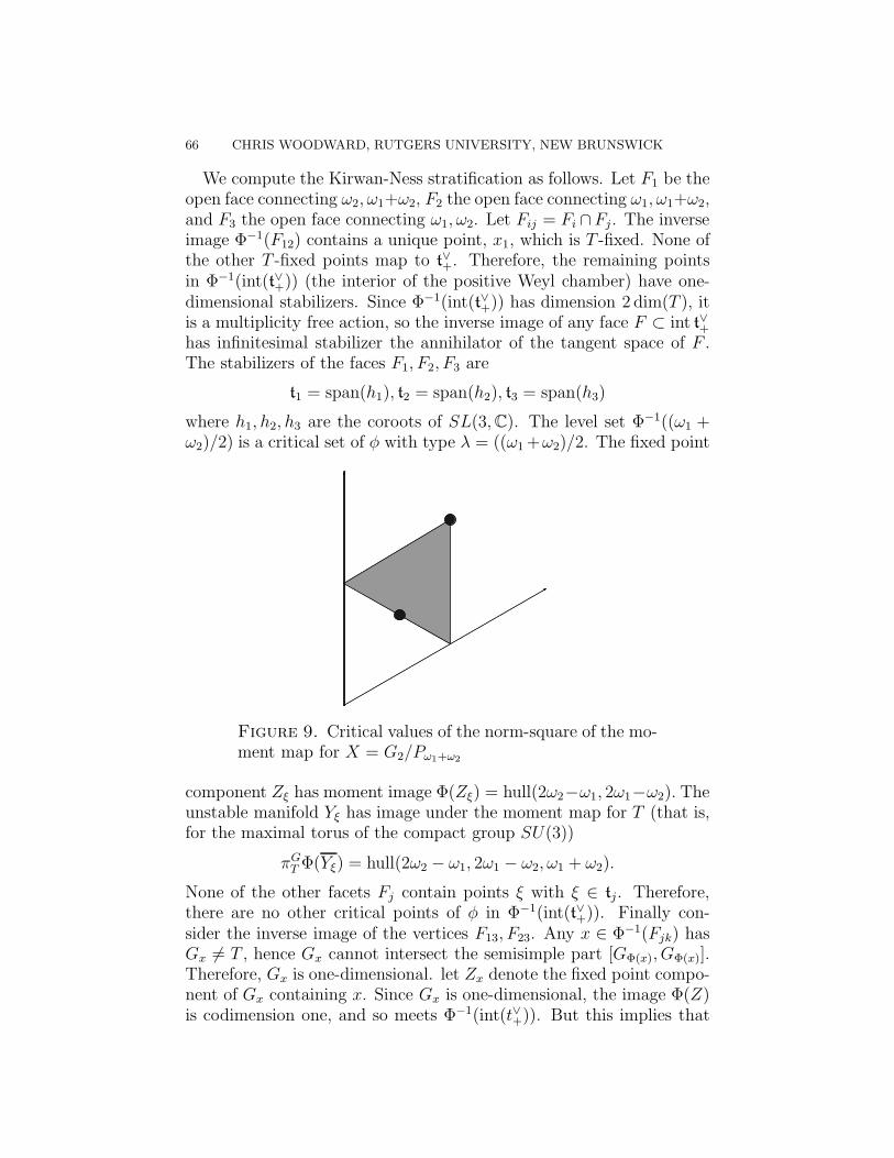
66 CHRIS WOODWARD, RUTGERS UNIVERSITY, NEW BRUNSWICK
We compute the Kirwan-Ness stratification as follows. Let F1 be theopen face connecting ω2, ω1+ω2, F2 the open face connecting ω1, ω1+ω2,and F3 the open face connecting ω1, ω2. Let Fij = Fi ∩Fj. The inverseimage Φ−1(F12) contains a unique point, x1, which is T -fixed. None ofthe other T -fixed points map to t∨+. Therefore, the remaining pointsin Φ−1(int(t∨+)) (the interior of the positive Weyl chamber) have one-dimensional stabilizers. Since Φ−1(int(t∨+)) has dimension 2 dim(T ), itis a multiplicity free action, so the inverse image of any face F ⊂ int t∨+has infinitesimal stabilizer the annihilator of the tangent space of F .The stabilizers of the faces F1, F2, F3 are
t1 = span(h1), t2 = span(h2), t3 = span(h3)
where h1, h2, h3 are the coroots of SL(3,C). The level set Φ−1((ω1 +ω2)/2) is a critical set of φ with type λ = ((ω1+ω2)/2. The fixed point
Figure 9. Critical values of the norm-square of the mo-ment map for X = G2/Pω1+ω2
component Zξ has moment image Φ(Zξ) = hull(2ω2−ω1, 2ω1−ω2). Theunstable manifold Yξ has image under the moment map for T (that is,for the maximal torus of the compact group SU(3))
πGT Φ(Yξ) = hull(2ω2 − ω1, 2ω1 − ω2, ω1 + ω2).
None of the other facets Fj contain points ξ with ξ ∈ tj. Therefore,there are no other critical points of φ in Φ−1(int(t∨+)). Finally con-sider the inverse image of the vertices F13, F23. Any x ∈ Φ−1(Fjk) hasGx 6= T , hence Gx cannot intersect the semisimple part [GΦ(x), GΦ(x)].Therefore, Gx is one-dimensional. let Zx denote the fixed point compo-nent of Gx containing x. Since Gx is one-dimensional, the image Φ(Z)is codimension one, and so meets Φ−1(int(t∨+)). But this implies that

MOMENT MAPS AND GEOMETRIC INVARIANT THEORY 67
the gx is conjugate to either tj or tk, and so gx cannot equal the spanof Fjk. Therefore, set of types for the action is ω1 + ω2,
12(ω1 + ω2).
(In fact the Kirwan-Ness stratification coincides with the orbit strati-fication for GC. That is, X is a two-orbit variety, with one open orbitand one of complex codimension two [33].)We now compute the contributions from the Kirwan-Ness strata.
For ξ = ω1 + ω2, Zssξ is equal to a point, and the bundle Nξ is the
representation with weights β5, β6. Hence
χGξ(Zss
ξ , E ⊗ Eul(Nξ)−1+ ) =
∑
(λ,α1)>k,(λ,α2)>k
zλ.
Its induction to G is
IndGGξχGξ
(Zssξ , E ⊗ Eul(Nξ)
−1+ ) =
∑
(λ,α1)>k,(λ,α2)>k
χλ.
For ξ = (ω1 + ω2)/2, we have Zssξ∼= C∗ and Nξ trivial. Therefore,
χGξ(Zss
ξ , E ⊗ Eul(Nξ)−1+ ) =
∑
(λ,ξ)≥k(ξ,ξ)
zλ
where the sum is over vectors λ such that λ − k(ω1 + ω2) is in somelattice Λ∨
1 , and satisfying the inequality above. Hence
IndGGξ(χGξ
(Zssξ , E ⊗ Eul(Nξ)
−1ξ )) =
∑
λ∈k∆
χλ −∑
(λ,α1)>k,(λ,α2)>k
χλ.
Since the contributions from ξ = (ω1+ω2),12(ω1+ω2) must have finite
sum, the lattice Λ∨1 must be the long root lattice. The contribution
(for k = 6) is shown in Figure 10.The positive contribution of the open stratum is finite (6 repre-
sentations, for k = 6) and the negative contribution infinite, that isdim(Hodd(Mξ, L
k)) = ∞, for any k. One can show that the highercohomology lies in H1, using the spectral sequence. The sum of thecontributions is χ(OX(k)) =
∑
λ∈k∆ χλ as claimed. This completes theexample.
Taking invariants in Theorem 10.4.1 gives a formula expressing thedifference between χ(X,E)G and χ(X//G,E//G):
Theorem 10.4.4.
χ(X,E)G−χ(X//G,E//G) =∑
λ6=0
χ(Zssλ , E|Zss
λ⊗Eul(NZss
λY ssλ )−1
+ ⊗Eul(g/p−λ ))Gλ
The spectral sequence also contains information about the individ-ual cohomology groups. For example, let C∗
λ ⊂ Gλ denote the one-parameter subgroup generated by λ. The weight ofC∗
λ on det(NXλX|Zss
λ)

68 CHRIS WOODWARD, RUTGERS UNIVERSITY, NEW BRUNSWICK
Figure 10. IndGT χZss
(ω1+ω2)/2,T (E)
is positive, if λ is non-trivial. Indeed, NXλX|Zss
λis the negative part of
the tangent bundle. Furthermore, g/p−λ has positive weights under C∗λ.
Thus
Corollary 10.4.5 (Teleman [104]). Suppose that the weights of C∗λ on
E|Zλ are positive for all types λ. (This is automatically the case ifE = OX(d) is the d-th tensor product of a polarization OX(1) of X).Then Hj(X,E)G = Hj(X//G,E//G) for all j.
In particular, if the higher cohomology of E vanishes then so does thatof E//G.The index maps naturally induce a diagram in K-theory
KG(X) K(X//G)
Z
s
which fails to commute by the above explicit sum of fixed point contri-butions for one-parameter subgroups. There are similar results in the

MOMENT MAPS AND GEOMETRIC INVARIANT THEORY 69
equivariant cohomology of X due to Paradan [88] and the author [113],based on earlier work of Witten [109]: a natural diagram of equivariantcohomology groups
HG(X) H(X//G)
R
s
fails to commute by an explicit sum of fixed point contributions fromone-parameter subgroups. The first explicit version of non-abelian lo-calization is due to Jeffrey-Kirwan [57], and expresses the difference asa sum over certain fixed point sets of the maximal torus. The versionsof Paradan, myself [113], and Beasley-Witten [11] express the differ-ence as a sum over critical points of the norm-square of the momentmap. The left hand arrow in the diagram above takes some work todefine: morally speaking it is defined by α 7→
∫
X×gα, but this is not
well-defined for polynomial equivariant classes. Rather, the left-handside must be defined by a suitable limit procedure, either by takingthe leading term in Riemann-Roch, or (in the context of equivariantde Rham cohomology with smooth coefficients) shifting by equivariantLiouville form and taking the zero limit of the shift, see [113]. Fromthis point of view, the K-theory approach is more natural.
References
[1] R. Abraham and J. Marsden. Foundations of Mechanics. Ben-jamin/Cummings, Reading, 1978.
[2] S. Agnihotri and C. Woodward. Eigenvalues of products of unitary matricesand quantum Schubert calculus. Math. Res. Lett., 5(6):817–836, 1998.
[3] D. N. Akhiezer. Lie group actions in complex analysis. Aspects of Mathemat-ics, E27. Friedr. Vieweg & Sohn, Braunschweig, 1995.
[4] Werner Ballmann, Mikhael Gromov, and Viktor Schroeder.Manifolds of non-positive curvature, volume 61 of Progress in Mathematics. Birkhauser BostonInc., Boston, MA, 1985.
[5] B. H. Bowditch. A class of incomplete non-positively curved manifolds. PacificJ. Math., 172(1):1–39, 1996.
[6] J. Arms, R. Cushman, and M. Gotay. A universal reduction procedure forHamiltonian group actions. In T. Ratiu, editor, The Geometry of HamiltonianSystems, volume 22 of Mathematical Sciences Research Institute Publications,Berkeley, 1989, 1991. Springer-Verlag, Berlin-Heidelberg-New York.
[7] M. F. Atiyah. Convexity and commuting Hamiltonians. Bull. London Math.Soc., 14:1–15, 1982.
[8] M. F. Atiyah and R. Bott. A Lefschetz fixed point formula for elliptic com-plexes. II. Applications. Ann. of Math. (2), 88:451–491, 1968.
[9] M. F. Atiyah and R. Bott. The moment map and equivariant cohomology.Topology, 23(1):1–28, 1984.

70 CHRIS WOODWARD, RUTGERS UNIVERSITY, NEW BRUNSWICK
[10] M. Audin. The Topology of Torus Actions on Symplectic Manifolds, volume 93of Progress in Mathematics. Birkhauser, Boston, 1991.
[11] C. Beasley and E. Witten. Non-abelian localization for Chern-Simons theory.J. Differential Geom., 70(2):183–323, 2005.
[12] P. Belkale. Local systems on P1 − S for S a finite set. Compositio Math.,129(1):67–86, 2001.
[13] P. Belkale and S. Kumar. Eigenvalue problem and a new product in cohomol-ogy of flag varieties. Invent. Math., 166(1):185–228, 2006.
[14] A. Berenstein and R. Sjamaar. Coadjoint orbits, moment polytopes, and theHilbert-Mumford criterion. J. Amer. Math. Soc., 13(2):433–466 (electronic),2000.
[15] A. Bialynicki-Birula. Some theorems on actions of algebraic groups. Ann. ofMath. (2), 98:480–497, 1973.
[16] A. M. Bloch and T. S. Ratiu. Convexity and integrability. In Symplectic geom-etry and mathematical physics (Aix-en-Provence, 1990), volume 99 of Progr.Math., pages 48–79. Birkhauser Boston, Boston, MA, 1991.
[17] R. Bott. Homogeneous vector bundles. Ann. of Math. (2), 66:203–248, 1957.[18] M. Brion. Sur l’image de l’application moment. In M.-P. Malliavin, editor,
Seminaire d’algebre Paul Dubreuil et Marie-Paule Malliavin, volume 1296 ofLecture Notes in Mathematics, pages 177–192, Paris, 1986, 1987. Springer-Verlag, Berlin-Heidelberg-New York.
[19] M. Brion. Groupe de Picard et nombres caracteristiques des varietesspheriques. Duke Math. J., 58(2):397–424, 1989.
[20] M. Brion, D. Luna, and Th. Vust. Espaces homogenes spheriques. Invent.Math., 84:617–632, 1986.
[21] M. Brion and M. Vergne. Lattice points in simple polytopes. J. Amer. Math.Soc., 10:371–392, 1997.
[22] L. Bruasse and A. Teleman. Harder-Narasimhan filtrations and optimaldestabilizing vectors in complex geometry. Ann. Inst. Fourier (Grenoble),55(3):1017–1053, 2005.
[23] A. Cannas da Silva. Introduction to symplectic and Hamiltonian geometry.Publicacoes Matematicas do IMPA. [IMPA Mathematical Publications]. In-stituto de Matematica Pura e Aplicada (IMPA), Rio de Janeiro, 2003.
[24] Pierre-Emmanuel Caprace and Alexander Lytchak. At infinity of finite-dimensional CAT(0) spaces. Math. Ann., 346(1):1–21, 2010.
[25] J. S. Carter, D. E. Flath, and M. Saito. The classical and quantum 6j-symbols.Princeton University Press, Princeton, NJ, 1995.
[26] X. Chen and S. Sun. Calabi flow, Geodesic rays, and uniqueness of constantscalar curvature Kahler metrics. arXiv:1004.2012.
[27] D. A. Cox. The homogeneous coordinate ring of a toric variety. J. AlgebraicGeom., 4(1):17–50, 1995.
[28] T. Delzant. Hamiltoniens periodiques et images convexes de l’application mo-ment. Bull. Soc. Math. France, 116:315–339, 1988.
[29] T. Delzant. Classification des actions Hamiltoniennes des groupes de rang 2.Ann. Global Anal. Geom., 8(1):87–112, 1990.
[30] S. K. Donaldson and P. Kronheimer. The geometry of four-manifolds. OxfordMathematical Monographs. Oxford University Press, New York, 1990.

MOMENT MAPS AND GEOMETRIC INVARIANT THEORY 71
[31] J. J. Duistermaat. Equivariant cohomology and stationary phase. In Symplec-tic geometry and quantization, (Sanda and Yokohama, 1993), volume 179 ofContemp. Math., pages 45–62, Providence, RI, 1994. Amer. Math. Soc.
[32] P. B. Eberlein. Geometry of nonpositively curved manifolds. Chicago Lecturesin Mathematics. University of Chicago Press, Chicago, IL, 1996.
[33] D. Feldmuller. Two-orbit varieties with smaller orbit of codimension two.Arch. Math. (Basel), 54(6):582–593, 1990.
[34] W. Fulton. Introduction to Toric Varieties, volume 131 of Annals of Mathe-matics Studies. Princeton University Press, Princeton, 1993.
[35] W. Fulton. Eigenvalues, invariant factors, highest weights, and Schubert cal-culus. Bull. Amer. Math. Soc. (N.S.), 37(3):209–249 (electronic), 2000.
[36] A. Grothendieck. Cohomologie locale des faisceaux coherents et theoremesde Lefschetz locaux et globaux (SGA 2). Documents Mathematiques (Paris)[Mathematical Documents (Paris)], 4. Societe Mathematique de France, Paris,2005. Seminaire de Geometrie Algebrique du Bois Marie, 1962, Augmented’un expose de Michele Raynaud. [With an expose by Michele Raynaud],With a preface and edited by Yves Laszlo, Revised reprint of the 1968 Frenchoriginal.
[37] V. Guillemin and S. Sternberg. Convexity properties of the moment mapping.Invent. Math., 67:491–513, 1982.
[38] V. Guillemin and S. Sternberg. Geometric quantization and multiplicities ofgroup representations. Invent. Math., 67:515–538, 1982.
[39] V. Guillemin and S. Sternberg. Homogeneous quantization and multiplicitiesof group representations. J. Funct. Anal., 47:344–380, 1982.
[40] V. Guillemin and S. Sternberg. Geometric Asymptotics, volume 14 of Mathe-matical Surveys and Monographs. Amer. Math. Soc., Providence, R. I., revisededition, 1990.
[41] V. Guillemin and S. Sternberg. Symplectic Techniques in Physics. CambridgeUniv. Press, Cambridge, 1990.
[42] V. W. Guillemin and S. Sternberg. Supersymmetry and equivariant de Rhamtheory. Springer-Verlag, Berlin, 1999. With an appendix containing tworeprints by Henri Cartan [MR 13,107e; MR 13,107f].
[43] V. Guillemin. Kaehler structures on toric varieties. J. Differential Geom.,40(2):285–309, 1994.
[44] V. Guillemin and R. Sjamaar. Convexity theorems for varieties invariant un-der a Borel subgroup. Pure Appl. Math. Q., 2(3, part 1):637–653, 2006.
[45] V. Guillemin and S. Sternberg. Multiplicity-free spaces. J. Differential Geom.,19(1):31–56, 1984.
[46] R. Hartshorne.Residues and duality. Lecture notes of a seminar on the work ofA. Grothendieck, given at Harvard 1963/64. With an appendix by P. Deligne.Lecture Notes in Mathematics, No. 20. Springer-Verlag, Berlin, 1966.
[47] J.-C. Hausmann and A. Knutson. The cohomology ring of polygon spaces.Ann. Inst. Fourier (Grenoble), 48(1):281–321, 1998.
[48] G. J. Heckman. Projections of orbits and asymptotic behavior of multiplicitiesfor compact Lie groups. Invent. Math., 67:333–356, 1982.
[49] P. Heinzner and F. Loose. Reduction of complex Hamiltonian G-spaces.Geom. Funct. Anal., 4(3):288–297, 1994.

72 CHRIS WOODWARD, RUTGERS UNIVERSITY, NEW BRUNSWICK
[50] P. Heinzner and A. Huckleberry. Kahlerian structures on symplectic reduc-tions. In Complex analysis and algebraic geometry, pages 225–253. de Gruyter,Berlin, 2000.
[51] S. Helgason. Differential geometry, Lie groups, and symmetric spaces. Aca-demic Press, New York, 1978.
[52] Wim H. Hesselink. Uniform instability in reductive groups. J. Reine Angew.Math., 303/304:74–96, 1978.
[53] Wim H. Hesselink. Desingularizations of varieties of nullforms. Invent. Math.,55(2):141–163, 1979.
[54] A. Horn. Doubly stochastic matrices and the diagonal of a rotation matrix.Amer. J. Math., 76:620–630, 1954.
[55] A. Horn. Eigenvalues of sums of Hermitian matrices. Pacific J. Math., 12:225–241, 1962.
[56] Ignasi Mundet i Riera. A Hilbert–Mumford criterion for polystability inKaehler geometry, 2008. arXiv.org:0804.1067.
[57] L. C. Jeffrey and F. C. Kirwan. Localization for nonabelian group actions.Topology, 34:291–327, 1995.
[58] V. A. Kaimanovich. Lyapunov exponents, symmetric spaces and a multiplica-tive ergodic theorem for semisimple Lie groups. Zap. Nauchn. Sem. Leningrad.Otdel. Mat. Inst. Steklov. (LOMI), 164(Differentsialnaya Geom. Gruppy Li iMekh. IX):29–46, 196–197, 1987.
[59] M. Kapovich, B. Leeb, and J. Millson. Convex functions on symmetric spaces,side lengths of polygons and the stability inequalities for weighted configura-tions at infinity. J. Differential Geom., 81(2):297–354, 2009.
[60] G. Kempf and L. Ness. The length of vectors in representation spaces. InK. Lonsted, editor, Algebraic Geometry, volume 732 of Lecture Notes in Math-ematics, pages 233–244, Copenhagen, 1978, 1979. Springer-Verlag, Berlin-Heidelberg-New York.
[61] F. C. Kirwan. Cohomology of Quotients in Symplectic and Algebraic Geom-etry, volume 31 of Mathematical Notes. Princeton Univ. Press, Princeton,1984.
[62] F. C. Kirwan. Convexity properties of the moment mapping, III. Invent.Math., 77:547–552, 1984.
[63] A. A. Klyachko. Equivariant vector bundles on toric varieties and some prob-lems of linear algebra. In Topics in algebra, Part 2 (Warsaw, 1988), pages345–355. PWN, Warsaw, 1990.
[64] F. Knop. Automorphisms of multiplicity free Hamiltonian manifolds.arXiv:1002.4256.
[65] F. Knop. The Luna-Vust theory of spherical embeddings. In Proceedings of theHyderabad Conference on Algebraic Groups (Hyderabad, 1989), pages 225–249, Madras, 1991. Manoj Prakashan.
[66] A. Knutson and T. Tao. The honeycomb model of gln(c) tensor products.
I. Proof of the saturation conjecture. J. Amer. Math. Soc., 12(4):1055–1090,1999.
[67] A. Knutson and T. Tao. Honeycombs and sums of Hermitian matrices.NoticesAmer. Math. Soc., 48(2):175–186, 2001.
MOMENT MAPS AND GEOMETRIC INVARIANT THEORY 73
[68] A. Knutson, T. Tao, and C. Woodward. The honeycomb model of GLn(C)tensor products. II. Puzzles determine facets of the Littlewood-Richardsoncone. J. Amer. Math. Soc., 17(1):19–48 (electronic), 2004.
[69] A. Knutson, T. Tao, and C. Woodward. A positive proof of the Littlewood-Richardson rule using the octahedron recurrence. Electron. J. Combin.,11(1):Research Paper 61, 18 pp. (electronic), 2004.
[70] B. Kostant. Quantization and unitary representations. In C. T. Taam, ed-itor, Lectures in Modern Analysis and Applications III, volume 170 of Lec-ture Notes in Mathematics, pages 87–208, Washington, D.C., 1970. Springer-Verlag, Berlin-Heidelberg-New York.
[71] Bertram Kostant. On convexity, the Weyl group and the Iwasawa decompo-
sition. Ann. Sci. Ecole Norm. Sup. (4), 6:413–455 (1974), 1973.[72] E. Lerman. Symplectic cuts. Math. Res. Letters, 2:247–258, 1995.[73] E. Lerman, E. Meinrenken, S. Tolman, and C. Woodward. Non-abelian con-
vexity by symplectic cuts. Topology, 37:245–259, 1998.[74] E. Lerman. Gradient flow of the norm squared of a moment map. Enseign.
Math. (2), 51(1-2):117–127, 2005.[75] I. V. Losev. Proof of the Knop conjecture. Ann. Inst. Fourier (Grenoble),
59(3):1105–1134, 2009.[76] D. Luna. Slices etales. Sur les groupes algebriques, Mem. Soc. Math. France,
33:81–105, 1973.[77] D. Luna and Th. Vust. Plongements d’espaces homogenes. Comment. Math.
Helv., 58(2):186–245, 1983.[78] I. G. Macdonald. Symmetric functions and Hall polynomials. Oxford Univer-
sity Press, New York, 1995. With contributions by A. Zelevinsky.[79] J. Marsden and A. Weinstein. Reduction of symplectic manifolds with sym-
metry. Rep. Math. Phys., 5:121–130, 1974.[80] E. Meinrenken. Symplectic surgery and the Spinc-Dirac operator. Adv. in
Math., 134:240–277, 1998.[81] K. Meyer. Symmetries and integrals in mathematics. In M. M. Peixoto, editor,
Dynamical Systems, Univ. of Bahia, 1971, 1973. Academic Press, New York.[82] D. Mumford, J. Fogarty, and F. Kirwan. Geometric Invariant Theory, vol-
ume 34 of Ergebnisse der Mathematik und ihrer Grenzgebiete, 2. Folge.Springer-Verlag, Berlin-Heidelberg-New York, third edition, 1994.
[83] M. S. Narasimhan and C. S. Seshadri. Stable and unitary vector bundles ona compact Riemann surface. Ann. of Math. (2), 82:540–567, 1965.
[84] L. Ness. A stratification of the null cone via the moment map. Amer. J. Math.,106(6):1281–1329, 1984. with an appendix by D. Mumford.
[85] P. E. Newstead. Introduction to moduli problems and orbit spaces, volume 51of Tata Institute of Fundamental Research Lectures on Mathematics andPhysics. Tata Institute of Fundamental Research, Bombay, 1978.
[86] P. E. Newstead. Geometric invariant theory. In Moduli spaces and vectorbundles, volume 359 of London Math. Soc. Lecture Note Ser., pages 99–127.Cambridge Univ. Press, Cambridge, 2009.
[87] T. Oda. Convex bodies and algebraic geometry, volume 15 of Ergebnisse derMathematik und ihrer Grenzgebiete (3) [Results in Mathematics and RelatedAreas (3)]. Springer-Verlag, Berlin, 1988. An introduction to the theory oftoric varieties, Translated from the Japanese.

74 CHRIS WOODWARD, RUTGERS UNIVERSITY, NEW BRUNSWICK
[88] P.-E. Paradan. The moment map and equivariant cohomology with general-ized coefficients. Topology, 39(2):401–444, 2000.
[89] P.-E. Paradan. Localization of the Riemann-Roch character. J. Funct. Anal.,187(2):442–509, 2001.
[90] S. Ramanan and A. Ramanathan. Some remarks on the instability flag. To-hoku Math. J. (2), 36(2):269–291, 1984.
[91] N. Ressayre. Geometric invariant theory and generalized eigenvalue problem.arXiv:0704.2127.
[92] J. Roberts. Asymptotics and 6j-symbols. Geom. Topol. Monogr., 4:245–261,2002. math.QA/0201177.
[93] A. H. W. Schmitt. Geometric invariant theory and decorated principal bun-dles. Zurich Lectures in Advanced Mathematics. European Mathematical So-ciety (EMS), Zurich, 2008.
[94] I. Schur. uber eine klasse von mittelbindungen mit anwendungen auf derdeterminanten theorie. S. B. Berlin Math. Ges., 22:9–20, 1923.
[95] J. -P. Serre. Representations lineaires et espaces homogenes kahleriens desgroupes de Lie compacts (d’apres Armand Borel et Andre Weil). In SeminaireBourbaki, Vol. 2, pages Exp. No. 100, 447–454. Soc. Math. France, Paris,1995.
[96] C. S. Seshadri. Fibres vectoriels sur les courbes algebriques, volume 96 ofAsterisque. Societe Mathematique de France, Paris, 1982. Notes written byJ.-M. Drezet from a course at the Ecole Normale Superieure, June 1980.
[97] S. S. Shatz. The decomposition and specialization of algebraic families ofvector bundles. Compositio Math., 35(2):163–187, 1977.
[98] G. C. Shephard. An elementary proof of Gram’s theorem for convex polytopes.Canad. J. Math., 19:1214–1217, 1967.
[99] R. Sjamaar. Holomorphic slices, symplectic reduction and multiplicities ofrepresentations. Ann. of Math. (2), 141:87–129, 1995.
[100] R. Sjamaar and E. Lerman. Stratified symplectic spaces and reduction. Ann.of Math. (2), 134:375–422, 1991.
[101] P. Slodowy. Die Theorie der optimalen Einparameteruntergruppen fur insta-bile Vektoren. In Algebraische Transformationsgruppen und Invariantentheo-rie, volume 13 of DMV Sem., pages 115–131. Birkhauser, Basel, 1989.
[102] G. Szekelyhidi. Extremal metrics and K-stability (PhD thesis).arxiv:math/0611002.
[103] A. Teleman. Symplectic stability, analytic stability in non-algebraic complexgeometry. Internat. J. Math., 15(2):183–209, 2004.
[104] C. Teleman. The quantization conjecture revisited. Ann. of Math. (2),152(1):1–43, 2000.
[105] R. P. Thomas. Notes on GIT and symplectic reduction for bundles and vari-eties. In Surveys in differential geometry. Vol. X, volume 10 of Surv. Differ.Geom., pages 221–273. Int. Press, Somerville, MA, 2006.
[106] G. Tian. On a set of polarized Kahler metrics on algebraic manifolds. J.Differential Geom., 32(1):99–130, 1990.
[107] Katrin Wehrheim and Chris T. Woodward. Functoriality for Lagrangian cor-respondences in Floer theory. Quantum Topol., 1:129–170, 2010.

MOMENT MAPS AND GEOMETRIC INVARIANT THEORY 75
[108] A. Weinstein. The symplectic “category”. In Differential geometric methodsin mathematical physics (Clausthal, 1980), volume 905 of Lecture Notes inMath., pages 45–51. Springer, Berlin, 1982.
[109] E. Witten. Two-dimensional gauge theories revisited. J. Geom. Phys., 9:303–368, 1992.
[110] E. Witten. Holomorphic Morse inequalities. In Algebraic and differentialtopology—global differential geometry, volume 70 of Teubner-Texte Math.,pages 318–333. Teubner, Leipzig, 1984.
[111] C. Woodward. The classification of transversal multiplicity-free group actions.Ann. Global Anal. Geom., 14:3–42, 1996.
[112] C. Woodward. Multiplicity-free Hamiltonian actions need not be Kahler. In-vent. Math., 131(2):311–319, 1998.
[113] C. T. Woodward. Localization via the norm-square of the moment map andthe two-dimensional Yang-Mills integral. J. Symp. Geom., 3(1):17–55, 2006.
[114] S. Wu. Equivariant holomorphic Morse inequalities. II. Torus and non-abeliangroup actions. J. Differential Geom., 51(3):401–429, 1999.
Mathematics-Hill Center, Rutgers University, 110 Frelinghuysen
Road, Piscataway, NJ 08854-8019, U.S.A.
E-mail address : [email protected]