Molecular Dynamics Simulations on High … 2 · M. Chiu and M.C. Herbordt ACM Reference Format:...

23

Molecular Dynamics Simulations onHigh-Performance ReconfigurableComputing Systems

MATT CHIU and MARTIN C. HERBORDTBoston University

The acceleration of molecular dynamics (MD) simulations using high-performance reconfigurablecomputing (HPRC) has been much studied. Given the intense competition from multicore andGPUs, there is now a question whether MD on HPRC can be competitive. We concentrate hereon the MD kernel computation: determining the short-range force between particle pairs. In onepart of the study, we systematically explore the design space of the force pipeline with respect toarithmetic algorithm, arithmetic mode, precision, and various other optimizations. We examinesimplifications and find that some have little effect on simulation quality. In the other part, wepresent the first FPGA study of the filtering of particle pairs with nearly zero mutual force, astandard optimization in MD codes. There are several innovations, including a novel partitioningof the particle space, and new methods for filtering and mapping work onto the pipelines. As aconsequence, highly efficient filtering can be implemented with only a small fraction of the FPGA’sresources. Overall, we find that, for an Altera Stratix-III EP3ES260, 8 force pipelines running atnearly 200 MHz can fit on the FPGA, and that they can perform at 95% efficiency. This resultsin an 80-fold per core speed-up for the short-range force, which is likely to make FPGAs highlycompetitive for MD.

Categories and Subject Descriptors: C.1.3 [Processor Architectures]: Other ArchitectureStyles—styles, heterogeneous (hybrid) systems, pipeline processors; J.3 [Life and MedicalSciences]: biology and genetics

General Terms: Algorithms, Design, Performance

Additional Key Words and Phrases: FPGA-based coprocessors, high performance reconfigurablecomputing, bioinformatics, biological sequence alignment, application acceleration

This work was supported in part by the NIH through award #R01-RR023168-01, by IBM througha Faculty Award and facilitated by donations from Altera Corporation.Preliminary versions of some of this work were presented at the 2nd Workshop on High Perfor-mance Reconfigurable Computing Technology and Applications (parts of Sections 3 and 6) andat the 19th International Conference on Field Programmable Logic and Applications (parts ofSections 4 and 5).Authors’ address: M. Chiu and M. C. Herbordt, Computer Architecture and Automated DesignLaboratory; Department of Electrical and Computer Engineering; Boston University; Boston, MA02215; Web: http://www.bu.edu/caadlab.Permission to make digital or hard copies part or all of this work for personal or classroom useis granted without fee provided that copies are not made or distributed for profit or commercialadvantage and that copies show this notice on the first page or initial screen of a display alongwith the full citation. Copyrights for components of this work owned by others than ACM must behonored. Abstracting with credit is permitted. To copy otherwise, to republish, to post on servers,to redistribute to lists, or to use any component of this work in other works requires prior specificpermission and/or a fee. Permissions may be requested from Publications Dept., ACM, Inc., 2 PennPlaza, Suite 701, New York, NY 10121-0701 USA, fax +1 (212) 869-0481, or [email protected]© 2010 ACM 1936-7406/2010/11-ART23 $10.00 DOI: 10.1145/1862648.1862653.

http://doi.acm.org/10.1145/1862648.1862653.

ACM Transactions on Reconfigurable Technology and Systems, Vol. 3, No. 4, Article 23, Pub. date: November 2010.

23: 2 · M. Chiu and M.C. Herbordt

ACM Reference Format:Chiu, M. and Herbordt, M. C. 2010. Molecular dynamics simulations on high performance recon-figurable computing systems. ACM Trans. Reconfig. Techn. Syst. 3, 4, Article 23 (November2010), 37 pages. DOI: 10.1145/1862648.1862653. http://doi.acm.org/10.1145/1862648.1862653.

1. INTRODUCTION

Molecular dynamics simulation (MD) is a central method in high-performance computing (HPC) with applications throughout engineering andnatural science. Acceleration of MD is a critical problem—there is a manyorder-of-magnitude gap between the largest current simulations and the po-tential physical systems to be studied. As such it has received attention as atarget for supercomputers [Fitch et al. 2006], clusters [Bowers et al. 2006],and dedicated hardware [Komeiji et al. 1997; Shaw et al. 2007; Taiji et al.2003], as well as coprocessing using GPUs [Rodrigues et al. 2008], Cell [Shi andKindratenko 2008], and FPGAs [Alam et al. 2007; Azizi et al. 2004; Gu et al.2006b; Hamada and Nakasato 2005; Kindratenko and Pointer 2006; Scrofanoand Prasanna 2006; Villareal et al. 2007]. The last of these, MD with High Per-formance Reconfigurable Computing (HPRC), is our focus here. In particular,we demonstrate that MD with HPRC is not only cost-effective, but in fact anexcellent fit. This result is surprising given the FPGA’s reputation for havingdifficulty with floating point intensive computations.

In this article we re-examine the short-range force computation which dom-inates MD. Although this problem has been addressed by many groups in thelast few years, much of the design space remains unexplored. In addition, re-cent advances in FPGA hardware and in compiler technology appear to haveshifted some basic trade-offs.

Our study has three parts. The first part considers the force pipeline. Ourgoal here is to maximize throughput—operating frequency and the number ofpipelines that fit on the FPGA—while maintaining simulation quality. To dothis, we explore various ways to perform the arithmetic, the modes in which toexecute the operations, the levels of precision, and other optimizations. Someof the choices are as follows.

—Direct computation (Direct) versus table lookup with interpolation (LookUp)—Interpolation order (for LookUp)—Precision: single, double, custom—Mode: floating point, hybrid fixed/floating point, custom—Implementation: synthesized components, vendor cores, vendor compiler

(e.g., Langhammer [2008])—Various arithmetic reorderings

We find that direct computation, rather than table lookup, is now preferred,and that single precision floating point combined with higher precision fixedpoint leads to both excellent performance and high-quality simulations.

The second part considers filtering particle pairs. This issue emergesfrom the geometric mismatch between two shapes: (i) the cubes (or otherACM Transactions on Reconfigurable Technology and Systems, Vol. 3, No. 4, Article 23, Pub. date: November 2010.

Molecular Dynamics Simulations on HPRCs · 23: 3

polyhedrons) into which it is convenient to partition the simulation space and(ii) the spheres around each particle in which the short-range force is non-zero.If this mismatch is not addressed (e.g., only the standard cell-list method isused), then 85.5% of the particle pairs that are run through the force pipelineswill be superfluous. While filtering is a critical issue, we believe that the onlypreviously published results related to hardware implementations are fromD.E. Shaw; these are with respect to their Anton processor [Larson et al. 2008].

Here, we find filtering implementation on FPGAs to provide a rich designspace. Its primary components are as follows.

—Filter algorithm and precision—Method of partitioning the cell neighborhood to balance load with respect to

the Newton’s-3rd-Law optimization—Method of mapping particle pairs to filter pipelines—Queueing and routing between filter and force pipelines

We present new algorithms or methods for filtering, load balancing, and map-ping, and find that nearly perfect filtering can be achieved with only a fractionof the FPGA’s logic.

The third part considers the integration of the new features specified by theother two parts. The particle mapping to the filter pipelines leads to changesin how cell lists are swapped on/off chip. Also, the filter pipelines generateneighbor lists which must be fed into the force pipelines. And having multipleforce pipelines (8 or more) requires accumulation of forces on the other end.We find solutions to all of these issues that have simple control, match FPGAresources, and add only little overhead.

Our basic result is that for the Stratix-III EP3SE260, and for the best (asyet unoptimized) designs, 8 force pipelines running at nearly 200 MHz can fiton the FPGA. Moreover, the force pipelines can be run at high efficiency with95% of cycles providing payload. As a result, the short-range force for the stan-dard 90K NAMD benchmark can be computed in under 22 ms, or about a fac-tor of 80 faster than its per-core execution time. Contributions are three-fold:(i) demonstrating that FPGAs are highly competitive for MD, (ii) substantiallyexpanding the exploration of the MD force pipeline design space for FPGAs,and (iii) presenting the first study of particle-particle filtering on FPGAs andwith it a number of innovations. The last of these may have implications to MDbeyond HPRC.

The rest of this article is organized as follows: In the next section, we reviewthe applicable parts of MD simulation. There follows the presentations of thethree parts of our study, after which come results and some discussion. Thisarticle builds on work presented at HPRCTA08 [Chiu et al. 2008] and FPL09[Chiu and Herbordt 2009] which concentrated on the force and filter pipelines,respectively. Besides combining and augmenting these pieces, we address herethe substantial issues of their integration, as well as data movement through-out the application: host-accelerator, board-FPGA, and among components onthe FPGA.ACM Transactions on Reconfigurable Technology and Systems, Vol. 3, No. 4, Article 23, Pub. date: November 2010.


2. MD PRELIMINARIES

2.1 MD Review

MD is an iterative application of Newtonian mechanics to ensembles of atomsand molecules (see, e.g., Rapaport [2004] for details). MD simulations generallyproceed in iterations each of which consists of two phases, force computationand motion integration. In general, the forces depend on the physical systembeing simulated and may include LJ, Coulomb, hydrogen bond, and variouscovalent bond terms:

Ftotal = Fbond + Fangle + Ftorsion + FHBond + Fnon−bonded (1)

Because the hydrogen bond and covalent terms (bond, angle, and torsion) af-fect only neighboring atoms, computing their effect is O(N) in the number ofparticles N being simulated. The motion integration computation is also O(N).Although some of these O(N) terms are easily computed on an FPGA, their lowcomplexity makes them likely candidates for host processing, which is what weassume here. The LJ force for particle i can be expressed as:

FL Ji =

∑j�=i

εab

σ 2ab

{12

(σab

|rji|)14

− 6(

σab

|rji|)8

}r ji (2)

where the εab and σab are parameters related to the types of particles, thatis, particle i is type a and particle j is type b . The Coulombic force can beexpressed as:

FCi = qi

∑j�=i

(q j

|r ji|3)

r ji (3)

A standard way of computing the nonbonded forces (LJ and Coulombic) is byapplying a cut-off. Then the force on each particle is the result of only particleswithin the cut-off radius rc. Since this radius is typically less than a tenth ofthe size per dimension of the system under study, the savings are tremendous,even given the more complex bookkeeping required.

The problem with cut-off is that, while it may be sufficiently accurate forthe rapidly decreasing LJ force, the error introduced in the slowly decliningCoulombic force may be unacceptable. A number of methods have been devel-oped to address this issue with some of the most popular being based on EwaldSums (see, e.g., Darden et al. [1993]) and multigrid (see, e.g., Izaguirre et al.[2005] and Skeel et al. [2002]). Here we use the standard convention of callingshort-range the LJ force and the Coulombic force generated within a cut-off ra-dius. We refer to the Coulombic force generated outside the cut-off radius aslong-range. Since the long-range force computation is generally a small frac-tion of the total (see, e.g., Gu and Herbordt [2007] and Scrofano and Prasanna[2006]), we concentrate here on the short-range force.

2.2 Short-Range Force Computation

As just described, the short-range force computation has two parts, the LJ forceand the rapidly converging part of the Coulomb force. The LJ force is oftenACM Transactions on Reconfigurable Technology and Systems, Vol. 3, No. 4, Article 23, Pub. date: November 2010.


computed with the so-called 6-12 approximation given in Eq. (2). This has twoterms, the repulsive Pauli exclusion and the van der Waals attraction. Bothrequire coefficients specific to the component particles of the particle pair whoseinteraction is being evaluated. These can be combined with the other constants(physical and scaling) and stored in coefficient look-up tables. Thus, the LJforce can be expressed as

FL Jji (rji(a, b ))

rji= Aab |rji|−14 + Bab |rji|−8 (4)

where Aab and Bab are distance-independent coefficient look-up tables indexedwith atom types a and b .

Returning now to the Coulomb force computation, we begin by rewritingEq. (3) as

FCLji (rji(a, b ))

rji= QQab |rji|−3, (5)

where QQab is a precomputed parameter (analogous to Aab and Bab ). Be-cause applying a cut-off here often causes unacceptable error, and also becausethe all-to-all direct computation is too expensive for large simulations, variousnumerical methods are applied to solve the Poisson equation that translatescharge distribution to potential distribution. To improve approximation qual-ity and efficiency, these methods split the original Coulomb force curve in twoparts (with a smoothing function ga(r)): a fast declining short range part and aflat long range part. For example:

1r

= (1r

− ga(r)) + ga(r). (6)

The short range component can be computed together with Lennard-Jonesforce using a third look-up table (for QQab ). The entire short range force tobe computed is:

Fshortji

rji= Aabr−14

ji + Babr−8ji + QQab (r−3

ji +g′

a(r)r

). (7)

2.3 Computing Short-Range Forces with Table Look-Up

Since these calculations are in the “inner loop,” considerable care is taken intheir implementation: even in serial codes, the LJ equation is often not evalu-ated directly, but rather with table look-up and interpolation. Previous imple-mentations of HPRC MD have used table look-up for the entire LJ force as afunction of particle separation [Azizi et al. 2004; Gu et al. 2006a]. The indexused is |rji|2 rather than |rji| so as to avoid the costly square-root operation.This method is efficient for uniform gases where only a single table is required[Azizi et al. 2004], but is less likely to be preferred in more general cases.

In more recent work [Gu et al. 2008], we use a different method: Instead ofimplementing the force pipeline with a single table lookup, we use three, oneACM Transactions on Reconfigurable Technology and Systems, Vol. 3, No. 4, Article 23, Pub. date: November 2010.


Fig. 1. Table look-up varies in precision across r−k. Each section has a fixed number of intervals.

each for r−14, r−8 and r−3ji + g′

a(r)r . Equation (7) can be rewritten as a function

of r2ji:

Fshortji (|rji|2(a, b ))

rji= Aab R14(|rji|2) + Bab R8(|rji|2) + QQab R3(|rji|2), (8)

where R14, R8, and R3 are lookup tables indexed with |rji|2.The intervals in the tables are represented in Figure 1. Each curve is divided

into several sections along the X-axis such that the length of each section istwice that of the previous. Each section, however, is cut into the same numberof intervals N. To improve the accuracy, higher order terms can be used. Whenthe interpolation is order M, each interval needs M + 1 coefficients, and eachsection needs N ∗ (M + 1) coefficients:

F(x) = a0 + a1x + a2x2 + a3x3 (9)

shows third order with coefficients ai. Accuracy increases with both the numberof intervals per section and the interpolation order. These issues are discussedin detail in Gu et al. [2008].

2.4 Filtering Particle Pairs

While MD in general involves all-to-all forces among particles, a cut-off is com-monly applied to restrict the extent of the short-range force to a fraction of thesimulation space. Two methods are used to take advantage of this cut-off: celllists and neighbor lists (see Figure 2). With cell lists, the simulation space istypically partitioned into cubes with edge-length equal to rc. Non-zero forces onthe reference particle P can then only be applied by other particles in its homecell and in the 26 neighboring cells (the 3x3x3 cell neighborhood). We refer thesecond particle of the pair as the partner particle. With neighbor lists, P hasassociated with it a list of exactly those partner particles within rc. We nowcompare these methods.

—Efficiency. Neighbor lists are by construction 100% efficient: only those parti-cle pairs with non-zero mutual force are evaluated. Cell lists as just definedare 15.5% efficient with that number being the ratio of the volumes of thecut-off sphere and the 27-cell neighborhood.

—Storage. With cell lists, each particle is stored in a single cell’s list. Withneighbor lists, each particle is typically stored in 400-1000 neighbor lists.



Fig. 2. Shown is part of the simulation space about particle P. Its two dimensional cell neighbor-hood is shown in white; cells have edge size equal to the cut-off radius. The cut-off circle is shown;particles within the circle are in P’s neighbor list.

—List Creation Complexity. Computing the contents of each cell requires onlyone pass through the particle array. Computing the contents of each neighborlist requires, naively, that each particle be examined with respect to everyother particle: the distance between them is then computed and thresholded.In practice, however, it makes sense to first compute cell lists anyway. Then,the neighbor lists can be computed using only the particles in each referenceparticle’s cell neighborhood.

From this last point, it appears that the creation of neighbor lists involvesnot only cell lists, but also a fraction of the force computation itself. At thispoint, why not finish computing the forces of those particles that are withinthe cut-off? Why save the neighbor list?

Most MD codes reuse the neighbor lists for multiple iterations and so amor-tize the work in their creation. But because particles move during each itera-tion, particles can enter and exit the cut-off region leading to potential error.The solution is to make the neighborlist cut-off larger than the force cut-off,for example, 13.5A versus 12A (see Figure 3). There is a trade-off between theincrease in neighborhood size, and thus the number of particle pairs evaluated,and the number of iterations between neighbor list updates.

3. FORCE PIPELINE DESIGN AND OPTIMIZATION

3.1 Overview

In this section, we describe FPGA implementations of Eq. (7). All are pipelinedand, on every cycle, input positions of particle pairs and output correspondingforces. There are numerous design axes as described in Section 1. The onesACM Transactions on Reconfigurable Technology and Systems, Vol. 3, No. 4, Article 23, Pub. date: November 2010.


Fig. 3. Neighborlists are often computed for a larger radius than the cutoff.

that reorder or change the pipeline components are as follows: the method ofcomputation, Direct versus table lookup with interpolation (LookUp); forLookUp, order of interpolation; for Direct, whether the Altera FP Compileris used or the FP cores directly; and whether integer is used for part of thecomputation.

The last two require further explanation. The Altera floating point compileroptimizes floating point datapaths by removing redundancy among operatorsand by making trade-offs in using various component types, for example, usinghard or soft components as available [Langhammer 2008]. What is interest-ing here is that the use of the compiler results in a different datapath beingoptimal.

The second axis requiring explanation is float versus hybrid fixed/float. Theproblem arises in the force accumulation at the end of the pipeline. New forcesare generated every cycle and must be added to the appropriate particles run-ning totals. The floating point addition, however, requires more than a singlecycle, although since it is pipelined it does not necessarily change throughput.But if the same particle’s force is referenced on successive cycles a hazard re-sults. There are at least four solutions: (i) the pipeline can stall, (ii) particleprocessing can be orchestrated so that hazards are avoided, (iii) forces can becombined in a more complex structure, such as a reduction tree, or (iv) theforce can be saved in integer format rather than floating point. In the last al-ternative, addition takes only a single cycle. Integer operations are also moreefficient than floating point, and if done carefully, result in no loss of precision.The GROMACS code and the Protein Explorer, for example, both use mixedfixed/floating point [Taiji et al. 2003; van der Spoel et al. 2005].

In the rest of this section, we show how these alternatives cause the forcepipeline to vary. Results are presented in Section 6.

3.2 Direct Computation

The flow of Direct is shown in Figure 4 with detail given in Figure 5. Notethat the first two computations, adjusting for periodic boundary conditions andACM Transactions on Reconfigurable Technology and Systems, Vol. 3, No. 4, Article 23, Pub. date: November 2010.


Fig. 4. Functional block diagram of the short-range particle-particle datapath.

obtaining r2, can be done in fixed point. In that case, r2 must be convertedto floating point before being combined with the coefficients (on the smoothingside) and divided (on the Coulomb + LJ side). The conversion at the output issimilar.

Figure 6 shows the Coulomb-plus-LJ block that is used with the compiler.An inverse square root replaces the original square root and divide saving logicand improving performance. This works because of the favorable convergenceproperties of the inverse square root.

3.3 Table Lookup with Interpolation

We now describe the interpolation pipeline (see Figure 7). Assuming that theinterpolation function is third order, it necessarily has the format

F(x) = ((C3(x − a) + C2)(x − a) + C1)(x − a) + C0,

where x ≡ r2 = input, a = the index of the interval from the beginningof the section (see Figure 1), and x − a = the offset into the interval. Thecoefficients C0, . . . , C3 are unique to each interval, and are retrieved byACM Transactions on Reconfigurable Technology and Systems, Vol. 3, No. 4, Article 23, Pub. date: November 2010.


Fig. 5. Shown is the detailed datapath for the direct computation. For hybrid integer/floatingpoint, the computation is the same, but with data before the first conversion and after the secondbeing integer.

determining the section and interval. Proper encoding makes trivial the ex-traction of the section, interval, and offset.

Figure 8 contains the replacement in Figure 5 needed to implement LookUp.For lower order interpolation, fewer stages are needed.ACM Transactions on Reconfigurable Technology and Systems, Vol. 3, No. 4, Article 23, Pub. date: November 2010.


Fig. 6. The Coulomb + LJ block (from Figure 5) modified for the FP Compiler optimization.

4. FILTER PIPELINE DESIGN AND OPTIMIZATION

We begin by assuming cell lists with processing concentrating on one home cellat a time. With no filtering or other optimization, forces are computed betweenall pairs of particles i and j, where i must be in the home cell but j can be in anyof the 27 cells of the cell neighborhood, including the home cell. By filtering, wemean the identification of particle pairs where the mutual short-range force iszero. A perfect filter successfully removes all such pairs. The efficiency of thefilter is the fraction of undesirable particle pairs removed. The extra work dueto imperfection is the ratio of undesirable pairs not removed to the desirablepairs.

We evaluate three methods, two existing and one new, which trade off filterefficiency for hardware resources. As motivated in Sections 3 and 6, we storeparticle positions in three Cartesian dimensions, each in 32-bit integer. Filterdesigns have two parameters, precision and geometry.

(1) Full Precision. Precision = full, Geometry = sphere. This filter computesr2 = x2 + y2 + z2 and compares whether r2 < r2

c using full 32-bit precision.Filtering efficiency is nearly 100%. Except for the comparison operation, thisis the same computation that is performed in the force pipeline.

(2) Reduced. Precision = reduced, Geometry = sphere. This filter, used byD.E. Shaw [Larson et al. 2008], also computes r2 = x2 + y2 + z2, r2 < r2

c , butuses fewer bits and so substantially reduces the hardware required. LowerACM Transactions on Reconfigurable Technology and Systems, Vol. 3, No. 4, Article 23, Pub. date: November 2010.


Fig. 7. The interpolation pipeline: the position of the leading 1 determines the operand format inthe interpolation pipeline.

precision, however, means that the cut-off radius must be increased (roundedup to the next bit) so filtering efficiency goes down: for 8 bits of precision, it is99.5% for about 3% extra work.

(3) Planar. Precision = reduced, Geometry = planes. A disadvantage of theprevious method is its use of multipliers, which are the critical resource in theforce pipeline. This issue can be important because there are likely to be 6 to10 filter pipelines per force pipeline. In this method we avoid multiplication bythresholding with planes rather than a sphere (see Figure 9 for the 2D analog).The formulae are as follows:

—|x| < rc, |y| < rc, |z| < rc—|x| + |y| <

√2rc, |x| + |z| <

√2rc, |y| + |z| <

√2rc

—|x| + |y| + |z| <√

3rc

With 8 bits, this method achieves 97.5% efficiency for about 13% extra work.ACM Transactions on Reconfigurable Technology and Systems, Vol. 3, No. 4, Article 23, Pub. date: November 2010.


Fig. 8. The Coulomb + LJ block (from Figure 5) modified for Table Lookup with Interpolation.Interpolation is 3rd order. Represented are three computations being done at once.

Analysis. Table I summarizes the cost (LUTs, registers, and multipliers) andquality (efficiency and extra work) of the three filtering methods. Since multi-pliers are a critical resource, we also show the two “sphere” filters implementedentirely with logic. The cost of a force pipeline (from Section 3) is shown forscale.

The most important result is the relative cost of the filters to the forcepipeline. Depending on implementation and load balancing method (seeSection 5.4), each force pipeline needs between 6 and 9 filters to keep it runningat full utilization. We refer to that set of filters as a filter bank. Table I showsthat a full precision filter bank takes from 80% and 170% of the resources ofits force pipeline. The reduced (logic only) and planar filter banks, however,require only a fraction: between 17% and 40% of the logic of the force pipelineand no multipliers at all. Since the latter is the critical resource, the conclusionis that the filtering logic itself (not including interfaces) has negligible effect onthe number of force pipelines that can fit on the FPGA.

We now compare the reduced and planar filters. The Extra Work column inTable I shows that for a planar filter bank to obtain the same performance aslogic-only-reduced, the overall design must have 13% more throughput. Thistranslates, for example, to having 9 force pipelines when using planar ratherthan 8 for reduced. The total number of filters remains constant. The choice offilter therefore depends on the FPGA’s resource mix.ACM Transactions on Reconfigurable Technology and Systems, Vol. 3, No. 4, Article 23, Pub. date: November 2010.


Fig. 9. Filtering with planes rather than a sphere – 2D analogue.

Table I. Comparison of Three Filtering Schemes with Respect to Quality and Resource Usage

Filtering Method LUTs/Registers Multipliers Filter Eff. Extra WorkFull precision 341/881 0.43% 12 1.6% 100% 0%Full prec. - logic only muls 2577/2696 1.3% 0 0.0% 100% 0%Reduced precision 131/266 0.13% 3 0.4% 99.5% 3%Reduced prec. - logic 303/436 0.21% 0 0.0% 99.5% 3%

only mulsPlanar 164/279 0.14% 0 0.0% 97.5% 13%Force pipe 5695/7678 5.0% 70 9.1% NA NA

A force pipeline is shown for reference. Percent utilization is with respect to the AlteraStratix-III EP3SE260.

5. MD SYSTEM DESIGN

5.1 Architecture of Target Systems

We briefly state our assumptions about the target HPRC architecture: They aretypical for current products; details of appropriate FPGA-based systems can befound, for example, in Hauck and DeHon [2008] and VanCourt and Herbordt[2009].

—The overall system consists of a host PC or workstation with an acceleratorboard plugged into a high-speed socket (e.g., PCI Express). The host runs themain application program and communicates with the accelerator throughfunction calls.

—The accelerator board consists of a high-end FPGA, memory, and a bus inter-face. On-board memory is tightly coupled to the FPGA either through severalinterfaces (e.g., 6 x 32-bit) or a wide bus (128-bit).



—Besides configurable logic, the FPGA has dedicated components such as in-dependently accessible multiport memories (e.g., 1000 x 1 KB) and a simi-lar number of multipliers. FPGAs in HPRC typically run at 200 MHz, al-though with optimization substantially higher operating frequencies can beachieved. We assume that 10%-15% of the FPGA’s logic is dedicated to sys-tem (nonapplication) functions such as memory controllers.

5.2 Host/Accelerator Partitioning

The filtering problem was introduced in Section 2.4 and filter designs given inSection 4. In this section, we present coprocessor-specific considerations andanswer the basic question of why perform filtering on the FPGA at all.

We begin with cell list computation: it is very fast and the data generatedsmall (both O(N)) so it is generally done on the host along with the motionintegration. Cell lists are downloaded to the coprocessor every iteration alongwith the new particle positions. The neighbor list computation, however, ismuch more expensive: if done on the host it could mitigate any advantage ofcoprocessing. Moreover, the size of the aggregate neighbor lists is often hun-dreds of times that of the cell lists, which makes their transfer impractical. Asa consequence, neighbor list computation, if it is done at all, must be done onthe coprocessor. But even on the coprocessor storage is still a concern.

We now look at MD operation starting with cell lists. For reference we ex-amine the NAMD benchmark NAMD2.6 on ApoA1. It has 92,224 particles, abounding box of 108A × 108A × 78A, and a cut-off radius of 12A. This yieldsa simulation space of 9 × 9 × 7 cells with an average of 175 particles per cellwith a uniform distribution. On the FPGA, the working set is typically a single(home) cell and its cell neighborhood for a total of (naively) 27 cells and about4,725 particles.

In actuality, Newton’s 3rd Law (N3L) is used to reduce this number. That is,since each particle-particle interaction is mutual, it is calculated once per par-ticle pair and recorded for both particles. To effect the reduction in work, homecell particles are only matched with particles of part of the cell neighborhood,and with, on average, half of the particles in the home cell. We refer to thesubset of cells in the cell neighborhood that are processed together with (andincluding) the home cell as the cell set. For the 14- and 18-cell sets presented inSection 5.4, the average number of particles to be examined (for each particlein the home cell) is 2,450 and 3,150, respectively. Given current FPGA tech-nology, any of these cell sets (14, 18, or the original 27 cells) easily fits in theon-chip BRAMs.

Neighbor lists for a home cell do not fit on the FPGA. For example, the ag-gregate of the neighbor lists for 175 home cell particles is over 64,000 particles(one half of 732 for each of the 175 particles; 732 rather than 4,725 because ofincreased efficiency of neighbor lists over cell lists).

The memory requirements are therefore very different for the two meth-ods. For cell lists, we swap cells onto and off of the FPGA as needed. Be-cause of the high level of reuse, this is commonly done in the background (seeSection 5.3). In contrast, neighbor list particles must be streamed from off-chip.ACM Transactions on Reconfigurable Technology and Systems, Vol. 3, No. 4, Article 23, Pub. date: November 2010.


This has worked when there are one or two force pipelines operating at 100MHz [Kindratenko and Pointer 2006; Scrofano et al. 2006], but is problematicfor current HPRC systems. For example, the Stratix-III/Virtex-5 generationof FPGAs supports 8 force pipelines operating at 200MHz leading to a band-width requirement of over 20 GB/s. While high-end FPGAs support this easily,memory interfaces in commercial systems generally do not.

From this discussion, it follows that use of neighbor lists calls for an “on-FPGA” solution, but that this itself appears to be impracticable due to memoryand transfer requirements. At the same time, however, the 6x potential in-crease in efficiency cannot be abandoned.

One way to improve efficiency is to reduce the cell size: the smaller the cellsize, the finer the granularity, and the larger the fraction of the cell neigh-borhood volume guaranteed to be useful. With a cell edge of rc/2 and a 53

set, efficiency increases to 26.8%. With more aggressive clipping of the cornercells, efficiency increases a bit more but so does the control complexity. Moreimportant is that reducing cell size also reduces reuse and still leaves muchinefficiency. While reducing cell size is viable, there are better options.

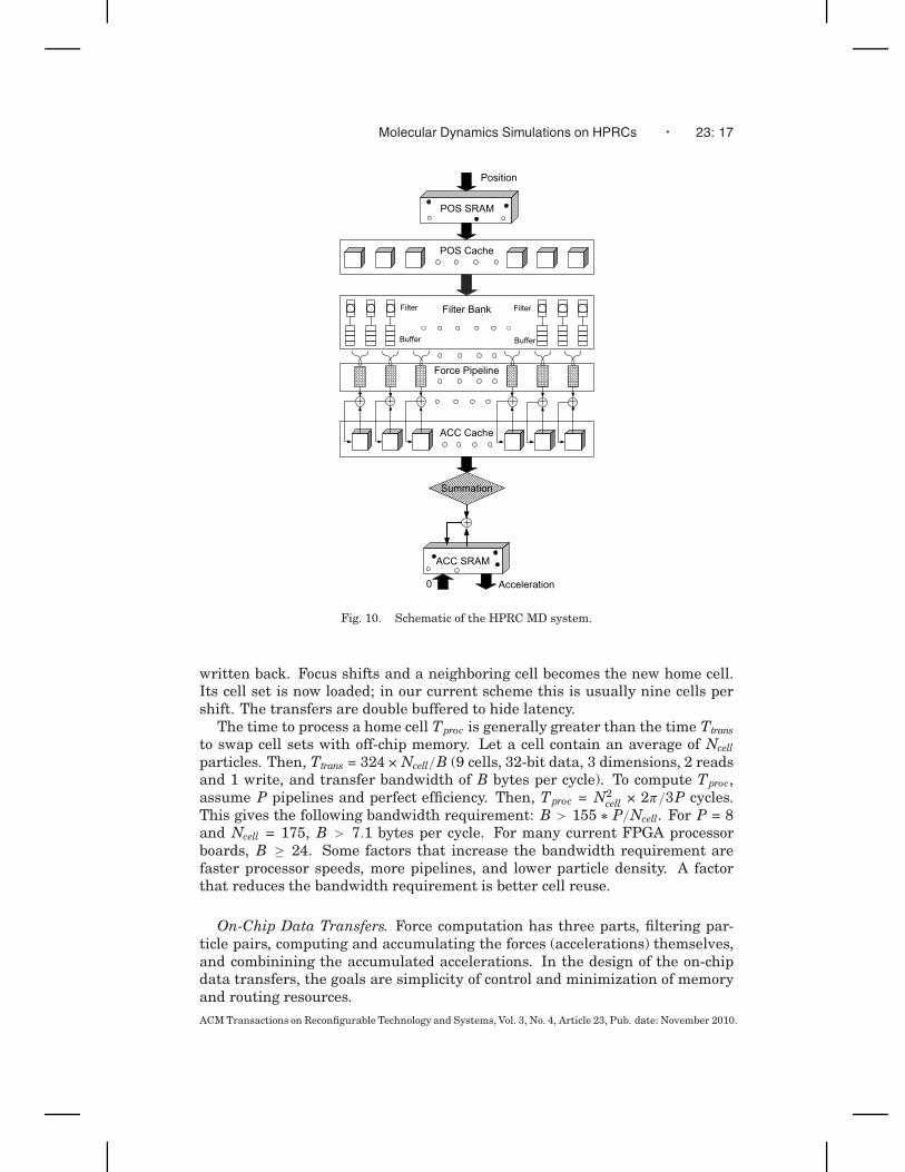
The solution we propose is to use neighbor lists, but to compute them everyiteration, generating them continuously and consuming them almost immedi-ately. In this scenario, the use of neighbor lists can be viewed as filtering outthe zero-force particle pairs: the filter pipelines feed the force pipelines withminimal buffering in between (see Figure 10).

5.3 Overall Design and Board-Level Issues

In this section, we describe the overall design (see Figure 10), especially howdata are transferred between host and accelerator and between off-chip andon-chip memory. Details of transfers from stage to stage are presented in thesucceeding subsections. For reference, we assume our current implementationof 8 force and 72 filter pipelines.

Host-Accelerator Data Transfers. At the highest level, processing is builtaround the timestep iteration and its two phases: force calculation and motionupdate. During each iteration, the host transfers position data to, and accel-eration data from, the coprocessor’s on-board memory (POS SRAM and ACCSRAM, respectively). With 32-bit precision, 12 bytes are transferred per parti-cle. While the phases are necessarily serial, the data transfers require only asmall fraction of the processing time. For example, in Section 6 the short-rangeforce calculation takes about 22 ms for 100-K particles and increases linearlywith particle count through the memory capacity of the board. The combineddata transfers of 2.4 MB take only 2-3ms. Moreover, since simulation proceedsby cell set, processing of the force calculation phase can begin almost immedi-ately as the data begin to arrive.

Board-Level Data Transfers. Force calculation is built around the process-ing of successive home cells. Position and acceleration data of the particles inthe cell set are loaded from board memory into on-chip caches, POS and ACC,respectively. When the processing of a home cell has completed, ACC data isACM Transactions on Reconfigurable Technology and Systems, Vol. 3, No. 4, Article 23, Pub. date: November 2010.


Fig. 10. Schematic of the HPRC MD system.

written back. Focus shifts and a neighboring cell becomes the new home cell.Its cell set is now loaded; in our current scheme this is usually nine cells pershift. The transfers are double buffered to hide latency.

The time to process a home cell Tproc is generally greater than the time Ttransto swap cell sets with off-chip memory. Let a cell contain an average of Ncell

particles. Then, Ttrans = 324× Ncell/B (9 cells, 32-bit data, 3 dimensions, 2 readsand 1 write, and transfer bandwidth of B bytes per cycle). To compute Tproc,assume P pipelines and perfect efficiency. Then, Tproc = N2

cell × 2π/3P cycles.This gives the following bandwidth requirement: B > 155 ∗ P/Ncell. For P = 8and Ncell = 175, B > 7.1 bytes per cycle. For many current FPGA processorboards, B ≥ 24. Some factors that increase the bandwidth requirement arefaster processor speeds, more pipelines, and lower particle density. A factorthat reduces the bandwidth requirement is better cell reuse.

On-Chip Data Transfers. Force computation has three parts, filtering par-ticle pairs, computing and accumulating the forces (accelerations) themselves,and combinining the accumulated accelerations. In the design of the on-chipdata transfers, the goals are simplicity of control and minimization of memoryand routing resources.ACM Transactions on Reconfigurable Technology and Systems, Vol. 3, No. 4, Article 23, Pub. date: November 2010.


Processing of a home cell proceeds in cohorts of reference particles that areprocessed simultaneously, either 8 or 72 at a time (either one per filter or oneper force pipeline, see Section 5.5). This allows a control with a single statemachine, minimizes memory contention, and simplifies accumulation. For thisscheme to run at high efficiency, two types of load-balancing are required: (i)the work done by various filter banks must be similar and (ii) filter banks mustgenerate particle pairs having non-trivial interactions on nearly every cycle.Details are given in the next subsections.

POS Cache to Filter Pipelines. Cell set positions are stored in 54-108BRAMS, that is, 1-2 BRAMs per dimension per cell. This number dependson the BRAM size, cell size, and particle density. Reference particles are al-ways from the home cell, partner particles can come from anywhere in the cellset. Given the flexibility in accessing the BRAMs there are a number of waysto organize these accesses (see, e.g., Figure 13).

Filter Pipelines to Force Pipelines. Various transfer schemes are describedin Section 5.6.

Force Pipelines to ACC Cache. To support N3L, two copies are made of eachcomputed force. One is accumulated with the current reference particle. Theother is stored by index in one of the large BRAMs on the Stratix-III. Accumu-lation is described in Section 5.7.

5.4 Balancing Neighbor List Sizes

For efficient access of particle memory and control, and for smooth interactionbetween filter and force pipelines, it is preferred to have each force pipelinehandle the interactions of a single reference particle at a time. This prefer-ence becomes critical when there are a large number of force pipelines and amuch larger number of filter pipelines. Moreover, it is highly desirable for allof the neighborlists being created at any one time (by the filter banks) to betransferred to the force pipelines simultaneously (buffering mechanisms aredescribed in Section 5.6). It follows that each reference particle should have asimilar number of partner particles (neighbor list size).

The problem addressed in this subsection is that the standard method ofchoosing a reference particle’s partner particles leads to a severe imbalance inneighbor list sizes. How this arises can be seen in Figure 11(a), which illus-trates the standard method of optimizing for N3L. So that a force between aparticle pair is computed only once, only a “half shell” of the surrounding cellsis examined (in 2D, this is cells 1–4 plus Home). For forces between the ref-erence particle and other particles in Home, the particle ID is used to breakthe tie, with, for example, the force being computed only when the ID of thereference particle is the higher. In Figure 11(a), particle B has a much smallerneighborlist than A, especially if B has a low ID and A a high.

In fact neighborlist sizes vary from 0 to 2L, where L is the average neigh-borlist size. The significance is as follows: Let all force pipelines wait for thelast pipeline to finish before starting work on a new reference particle. Then,ACM Transactions on Reconfigurable Technology and Systems, Vol. 3, No. 4, Article 23, Pub. date: November 2010.


Fig. 11. Shown are two partitioning schemes for using Newton’s 3rd Law. In (a), 1-4 plus homeare examined with a full sphere. In (b), 1-5 plus home are examine, but with a hemisphere (shadedpart of circle).

Fig. 12. Distribution of neighborlist sizes for standard partition as derived from Monte Carlosimulations.

if that (last) pipeline’s reference particle has a neighborlist of size 2L, thenthe latency will be double that if all neighbor lists were size L. This dis-tribution has high variance (see Figure 12), meaning that neighbor list sizesgreater than, say, 3

2 L are likely to occur. A similar situation also occurs inother MD implementations, with different architectures calling for differentsolutions [Anderson et al. 2008; Snir 2004].

One way to deal with this load imbalance is to overlap the force pipelinesso that they work independently. While viable, this leads much more complexcontrol.ACM Transactions on Reconfigurable Technology and Systems, Vol. 3, No. 4, Article 23, Pub. date: November 2010.


An alternative is to change the partitioning scheme. Our new N3L partitionis shown in Figure 11(b). There are three new features. The first is that the cellset has been augmented from a half shell to a prism. In 2D, this increases thecell set from 5 cells to 6; in 3D, the increase is from 14 to 18. The second is that,rather than forming a neighbor list based on a cutoff sphere, a hemisphere isused instead (the “half-moons” in Figure 11(b)). The third is that there is nowno need to compare IDs of home cell particles.

We now compare the two partitioning schemes. There are two metrics: theeffect on the load imbalance and the extra resources required to prevent it.

(1) Effect of Load Imbalance. We assume that all of the force pipelines begincomputing forces on their reference particles at the same time, and that eachforce pipeline waits until the last force pipeline has finished before continuingto the next reference particle. We call the set of neighbor lists that are thusprocessed simultaneously a cohort. With perfect load balancing, all neighborlists in a cohort would have the same size, the average L. The effect of thevariation in neighbor list size is in the number of excess cycles—before a newcohort of reference particles can begin processing—over the number of cyclesif each neighborlist were the same size. The performance cost is therefore theaverage number of excess cycles per cohort. This in turn is the average sizeof the biggest neighbor list in a cohort minus the average neighbor list size.We find that, for the standard N3L method, the average excess is nearly 50%,while for the “half-moon” method it is less than 5%.

(2) Extra Resources. The extra work required to achieve load balance is pro-portional to the extra cells in the cell set: 18 versus 14, or an extra 29%. Thisdrops the fraction of neighbor list particles in the cell neighborhood from 15.5%to 11.6%, which in turns increases the number of filters needed to keep theforce pipelines fully utilized (overprovisioned) from 7 to 9. For the reduced andplanar filters, this is not likely to reduce the number of force pipelines.

5.5 Mapping Particle Pairs to Filter Pipelines

From the previous sections, we converge on an efficient design for filteringparticle pairs.

—During execution, the working set (data held on the FPGA) consists of thepositions and accelerations of particles in a cell set; that is, a single homecell and its 17 neighbors (in the “half moon” scheme);

—Particles from each cell are stored in a set of BRAMs: this is currently one ortwo BRAMs per coordinate, depending on the cell size, for a total of 108-216;

—The N3L partition specifies 7-9 filter pipelines per force pipeline;—FPGA resources in the Stratix-III/Virtex-5 generation yield 8-10 force

pipelines; and—Force pipelines handle at most a small number of reference particles at a

time (and their N3L partners).

We now address the mapping of particle pairs to filter pipelines. There area (perhaps surprisingly) large number of ways to do this; finding the optimalACM Transactions on Reconfigurable Technology and Systems, Vol. 3, No. 4, Article 23, Pub. date: November 2010.


Fig. 13. Two mappings of particle pairs onto filters. (a) Particle Mapping: Filters each hold adifferent reference particle. Particles in cell set are broadcast one per cycle. (b) Cell Mapping:Same reference particle held by all filters in a bank. Each filter is responsible for 2-3 cells.

mapping is in some ways analogous to optimizing loop interchanges with re-spect to a cost function. Figure 13 shows two possibilities. In particle mapping(a), each filter is responsible for a different reference particle. Each cycle, a sin-gle partner particle from the cell set is broadcast to all of the filters (in all of thefilter banks). In cell mapping (b), each filter bank is collectively responsible fora different reference particle. Each filter within a bank processes the referenceparticle with respect to partners from its own subset of 2 or 3 cells. The issuesare as follows:

Force Pipeline Efficiency. Overall performance is proportional to the effi-ciency of the force pipelines, that is, the fraction of cycles that they deliver“payload” (pairs with non-zero forces). Since there are no stalls, the efficiencyis thus proportional to the fraction of cycles that they input (are issued) payloadparticle pairs from their filter banks.

Payload Generation Rate. Given sufficient filters, a filter bank will generatepayload pairs at an average rate of greater than one per cycle. The variancemay be high, however, which can substantially degrade efficiency.

Distribution of Payload Particle Pairs. While the number of payload par-ticle pairs from a given cell set—and even from any reference particle (fromSection 5.4)—has a small variance, the number and distribution of payloadpairs generated by any particular filter can vary wildly. For example, inFigure 11(b), let two filters (in a bank) each handle the same reference par-ticle, but let the partner particles be from different cells, say 3 and 5. Eachfilter examines the same number of pairs, but the first filter passes most of itsinput while the second passes almost none.

Queueing Particle Pairs. A simple (but costly) solution is to: (i) append alarge queue to each filter and (ii) implement a flexible router from these queuesACM Transactions on Reconfigurable Technology and Systems, Vol. 3, No. 4, Article 23, Pub. date: November 2010.


to the force pipeline. The two mappings lend themselves to multiple more prac-tical queueing methods, the choice of which depends on the resources availableon the FPGA.

In the next section we present two queueing strategies, whole neighborlistand continuous. We evaluate them with respect to the two particle mappingstrategies for performance (force pipeline efficiency) and hardware cost (queuesize and complexity).

5.6 The Filter Pipeline – Force Pipeline Interface

If there are sufficient BRAMs, then particle mapping can be used to generateneighborlists in their entirety; they are consumed in the same way. Details areas follows.

—A phase begins with a new and distinct reference particle being associatedwith each filter.

—Then, on each cycle, a single particle from the 18-cell set is broadcast to allof the filters.

—Each filter’s output goes to its own set of BRAMs.—The output of each filter is exactly the neighborlist for its associated reference

particle.—Double buffering enables neighborlists to be generated by the filters at the

same time that the previous phase’s neighborlists are being drained by theforce pipelines.

Advantages of this method include:

—Nearly perfect load balance among the filters (from the “half-moon” parti-tion);

—Little overhead: each phase consists of over 3000 cycles before a new set ofreference particles must be loaded;

—Nearly perfect load balancing among the force pipelines: each operates suc-cessively on a single reference particle and its equal-sized neighborlist; and

—Simple queueing and control: neighborlist generation is decoupled from forcecomputation.

One disadvantage of the whole neighborlist method is that it requires hun-dreds of BRAMs. Although there are a thousand or more on some high-endFPGAs, this is still a concern. Another disadvantage is fragmentation. Thenumber of phases necessary to process the particles in a single home cell is�|particles-in-home-cell| / |filters|. For small cells or low-density simulations,the loss of efficiency can become significant. There are, however, several rea-sonable solutions.

—Increase the number of filters and further decouple neighbor list generationfrom consumption. The reasoning is that as long as the force pipelines arebusy, some inefficiency in filtering is acceptable.



—Overlap processing of two home cells. This increases the working set from 18to 27 cells for a modest increase in number of BRAMs required. One way toimplement this is to add a second distribution bus.

—Another way to overlap processing of two home cells is to split the filtersamong them. This halves the phase granularity, and so the expected inef-ficiency, without significantly changing the amount of logic required for thedistribution bus.

For the rest of this section, we examine more direct transfers of data fromfilters to force pipelines. Figure 13 shows the basic queueing used in both map-pings: Some number of filters Nfilters in a filter bank feed a single force pipeline.Each filter has a queue to which it outputs its data. As described in Section 5.3,the force pipelines should be as independent from one another as possible. Thisis to constrain the complexity of the routing between filter and force stages andbetween force stage and ACC Cache.

At a high-level, this is a typical queueing problem with Nfilters servers whereeach has known arrival and departure rates. An arrival is the generation of aparticle pair that has passed the filter criteria; a departure is when a payloadpair is consumed by the force pipeline. Also, the goal is to minimize idle time(when all of the queues are empty) and hardware cost. The latter includesqueue size, but also complexity of the control and of the concentrator logic thatroutes from the filter queues to the force pipeline.

There are also a number of differences, however. These restrict the utility ofstochastic analysis, but also point to implementation methods.

(1) Execution Proceeds in Phases. For particle mapping, the filter bankprocesses a cohort of Nfilters reference particles in a phase. For cell map-ping, it processes a single reference particle.

(2) Uniformity. The total number of arrivals per reference particle varies onlyslightly within a phase (for particle mapping) and among phases (for bothmappings).

(3) Nonuniformities. The Nfilters queues can have highly non-uniform depar-ture rates and/or high variation in departure rates during a phase. De-pending on the position of the reference particle in the home cell and on thecell of its partner, the a priori probability of a departure can be anythingfrom 0 to 1.

Some design considerations are as follows: To minimize queue size, thereare several mechanisms including under provisioning (by keeping Nfilters small)and throttling (when queues are full). Even if these are used, however, perfor-mance is improved by smoothing and balancing the departure rates (arrivalsat the force pipelines). Here are three ways that help do this.

Fetch Order. Especially for particle mapping, departure rates for each filtervary considerably during a phase. For example, in Figure 11(b), the filter (ofthe particle shown) has a departure rate near 0 when cell 4 is processed, butgreater than .5 for cell 3. This variation can be smoothed by randomizing theorder in which the partner particles are fetched from the cell set. A simpleACM Transactions on Reconfigurable Technology and Systems, Vol. 3, No. 4, Article 23, Pub. date: November 2010.


Fig. 14. Concentrator logic between filters and force pipeline.

way to approximate this is to fetch particles from cells round-robin rather thancell-at-a-time.

Mapping Combinations of Cells. For cell mapping, different cells in the cellset vary widely in the probability that their particles will be part of a neighborlist. For example, in Figure 11(b), the Home cell and cell 3 are much more likelyto provide payload partner particles than the corner cells (2 and 4). Pairingcells appropriately, for example, one with much payload potential with one thathas little, helps equalize the arrival rates.

Concentrator Logic. Complex logic can completely smooth non-uniformitiesamong filter queue arrivals (within a cycle) by transferring them to the queueswith the most space. Logic that provides a nearly the same effectiveness butwith minimal hardware cost is shown in Figure 14. Each filter independentlyenqueues particle pairs that have passed the selection criteria. An arbiter de-termines transfer to the force pipeline based on the following logic.

(1) First priority is given to queues that are within one of being full. This issufficient to prevent data from being dropped. If multiple queues are nearlyfull, then priority is rotated round-robin.

(2) Otherwise, priority is given to queues that are not empty. Again, priority isrotated round-robin.

(3) If multiple queues are nearly full, then the filters are throttled. Note thatthrottling by itself does not reduce efficiency; the key performance consid-eration is that the force pipelines always be active.

Another design consideration is whether to over- or under-provision andwhether to throttle filter pipeline input to reduce the queue size needed toprevent overflow. Having a smaller or larger number of filters under- orover-provisions the force pipeline. The advantage of under-provisioning is thatACM Transactions on Reconfigurable Technology and Systems, Vol. 3, No. 4, Article 23, Pub. date: November 2010.


Table II. Queue Size Requirement and Utilization are Shown forVarious Configurations with No Throttling

particle mapped cell mapped# of filters 6 7 8 9 6 9Queue size 10 18 36 80 6 36Utilization 69.7% 81.2% 92.5% 99.3% 69.6% 98.3%

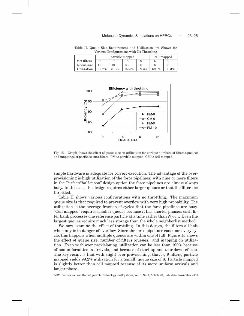
Fig. 15. Graph shows the effect of queue size on utilization for various numbers of filters (queues)and mappings of particles onto filters. PM is particle mapped, CM is cell mapped.

simple hardware is adequate for correct execution. The advantage of the over-provisioning is high utilization of the force pipelines: with nine or more filtersin the Perfect/“half-moon” design option the force pipelines are almost alwaysbusy. In this case the design requires either larger queues or that the filters bethrottled.

Table II shows various configurations with no throttling. The maximumqueue size is that required to prevent overflow with very high probability. Theutilization is the average fraction of cycles that the force pipelines are busy.“Cell mapped” requires smaller queues because it has shorter phases: each fil-ter bank processes one reference particle at a time rather than Nfilters. Even thelargest queues require much less storage than the whole neighborlist method.

We now examine the effect of throttling. In this design, the filters all haltwhen any is in danger of overflow. Since the force pipelines consume every cy-cle, this happens when multiple queues are within one of full. Figure 15 showsthe effect of queue size, number of filters (queues), and mapping on utiliza-tion. Even with over provisioning, utilization can be less than 100% becauseof nonuniformities in arrivals, and because of start-up and tear-down effects.The key result is that with slight over provisioning, that is, 9 filters, particlemapped yields 99.2% utilization for a (small) queue size of 8. Particle mappedis slightly better than cell mapped because of its more uniform arrivals andlonger phase.ACM Transactions on Reconfigurable Technology and Systems, Vol. 3, No. 4, Article 23, Pub. date: November 2010.


Fig. 16. Mechanism for accumulating per particle forces. (a) shows the logic for a single pipelinefor both the reference and partner particles. (b) shows how forces are accumulated across multiplepipelines.

5.7 Accumulating and Combining the Accelerations

The final processing steps are accumulating and combining the accelerationsgenerated by the force pipelines. Unlike position data, which is read only, ac-celeration data is read/write. That is, during the processing of a home cell,each particle’s acceleration accumulates over this and other cells in the cell set;it is not complete until all 27 cells in the neighborhood have taken a turn asthe home cell. Thus for each new home cell, the running total of accumulatedaccelerations of the cell set are read onto the chip in a way analogous to theposition data.

One design constraint is that each force pipeline handles at most a smallnumber of reference particles Pi at a time. This enables the total forces onthe Pis to be accumulated in registers. Accumulating the mutual forces on thePis’ N3L partner particles (Pjs), however, is more complex as their positionsspan the cell set. To prevent BRAM access contention, the following strategyis used. Partner updates are written to BRAMs associated uniquely with eachforce pipeline. When processing of a home cell is completed, the partner datafrom the various pipeline-specific BRAMs are merged.

This method is depicted in Figure 16. In (a), the running accumulation fora single pipeline during cell processing is shown. We describe this for parti-cle mapping, cell mapping is analogous. Recall that each of the Nforce forcepipelines has Nfilters filters and that each filter processes a unique referenceparticle at a time. Also that reference particles are always from the home cell,but that partner particles come from the entire cell set. For each force pipeline,there are Nfilters accumulators for the Nfilters reference particles being processedat a time. There are also Nforce force caches, one for each pipeline. Each forcecache has an accumulator for each particle in the entire cell set.

Processing proceeds as follows: A new home cell and its acompanying cellset (positions and accelerations) are loaded. From the home cell, a cohort ofreference particles is loaded into the filters. Forces are now computed withrespect to all of the cell set particles and sent to the accumulators. Each force(for particle pair i, j) is added to both the register corresponding to referenceparticle i and to the jth slot in that force pipeline’s force cache. The accesses tothe force cache BRAMs are pipelined: the js are sent a few cycles ahead so thatthe current accumulated values are available “just in time.” When the cohort ofACM Transactions on Reconfigurable Technology and Systems, Vol. 3, No. 4, Article 23, Pub. date: November 2010.


reference particles has been processed, the reference particle accumulators inthe force array are combined with those in the force cache. When the home cellhas been processed, the Nforce force caches are combined (see Figure 16(b); thebasic design first appeared in Gu [2008]). This operation is performed duringswapping out, so its latency is completely hidden.

6. RESULTS

6.1 Overview

We use NAMD [Phillips et al. 2002] and ProtoMol [Matthey 2004] as referencecodes, both to determine the number of short-range particle-particle interac-tions computed per iteration as well as the microprocessor time (per iterationper core). NAMD scales well with multiple cores and multiple processors up tohundreds of processors.

We refer to the NAMD benchmark NAMD2.6 on ApoA1. It has 92,224 par-ticles, a bounding box of 108A × 108A × 78A, and a cut-off radius of 12A.By instrumenting the codes, we determine that on average 33.4M non-trivialparticle-particle computations are performed per iteration. This agrees veryclosely with the 33.75M computations expected from the analysis in Section 5.2.According to a study by Stone et al. [2007], this benchmark is executed at 1.78seconds per iteration on a single core of an Intel core 2 quad-core 2.66 GHzprocessor.

The rest of this section is organized as follows: In the next two sections,we evaluate the force pipelines proposed in Section 3. We do this first for re-source utilization and then for simulation quality. In the final subsection, wedescribe current status of the overall implementation and implications for MDon HPRC.

6.2 Performance Comparisons of Force Pipeline Design Alternatives

Results are through post place-and-route (PaR) using the standard Altera toolchain. We assume the Stratix-III EP3SE260. This method is sufficient to giveprecisely the resource usage and the number of pipelines. For operating fre-quency, true implementations are often slightly lower. On the other hand, thefloating point cores (and code compiled using the Altera Floating Point Com-piler or FPC) are specified to run at more than 250 MHz, so with some op-timization higher performance than what we have achieved so far could berealized. We first present the best design; it is characterized as follows.

—Direct computation (no table look-up)—Hybrid fixed and floating point—Single precision except for force accumulation (36 bit)—Generated using FPC

(1) Hybrid versus Single Precision versus Double Precision. Figure 17 showsresource usage for a number of arithmetic modes and force pipeline designs.Hybrid uses 32-bit fixed point for displacement and 36-bit fixed point for forceACM Transactions on Reconfigurable Technology and Systems, Vol. 3, No. 4, Article 23, Pub. date: November 2010.


Fig. 17. Resource utilization in registers and logic for the Stratix-III. LUT3 is LookUp with 3rdorder interpolation. DIR is Direct. HYB refers to Direct with partial fixed point.

accumulation. Single and double refer to use of floating point throughout.SemiFP is described in detail in previous work [Gu et al. 2008]; it has 35 bitsof precision. Not shown here is that LookUp requires significant use of BRAMs(to hold the tables) while Direct does not.

We observe that while Stratix-III FPGAs have substantial floating point sup-port, this does not result in direct scaling from single to double precision. Theincrease in resources required is 2.5× - 3× for logic, but 4× - 4.5× for the mul-tipliers. Also, the operating frequency is reduced, but the quality improves.

(2) Effect of Arithmetic Implementation. Figure 18 shows the resource usageof various implementations but this time emphasizing single precision and thevariation in interpolation order in LookUp.

Direct computation (DC) uses less than 10% of the DSP units and far less ofthe remaining logic. The 3rd order LookUp uses a similar fraction of DSP units,but substantially more logic. Reducing the interpolation order to 2nd and 1stallows the implementation of perhaps another pipeline or two, but may not beworth the decrease in simulation quality. Overall, this is a surprising result.In previous studies we found LookUp to be superior to Direct. We attribute thechange to advances in floating point support in both the FPGA hardware andthe tool chain (cores and floating point compiler).

(3) Floating Point Compiler versus Core Only. The effect of using the AlteraFloating Point Compiler is shown in Figure 19. This computation (short-rangeforce pipeline) does not take advantage of most of the compiler optimizations,but still results in a substantial reduction in non-DSP logic. This is especiallyhelpful for saving logic for the filter pipelines.ACM Transactions on Reconfigurable Technology and Systems, Vol. 3, No. 4, Article 23, Pub. date: November 2010.


Fig. 18. Resource utilization in registers and logic for the Stratix-III. The LUT number refers tothe order of the interpolation. LUT implementations are for single precision FP.

Fig. 19. Effect of using the Altera FPC on logic utilization. For single pipeline, single precision.Same configurations as in Figure 18.

6.3 Quality Comparisons of Design Alternatives

Direct evaluations of MD simulation quality, such as through validation withwet-lab experiments, are often impractical. Thus surrogates are often used.One type measures the errors with respect to a reference computation. Anothertype monitors the simulation output to confirm that a physical invariant, suchas the total energy, actually is so. Here we use two of each type.ACM Transactions on Reconfigurable Technology and Systems, Vol. 3, No. 4, Article 23, Pub. date: November 2010.


Fig. 20. Relative average force error for the particle-particle force computation for various imple-mentations and precisions. DIR is direct computation, LUTn refers to LookUp of various orders.

(1) Error per Individual Particle-Particle Force Computation. Figure 20shows the relative average error for the individual particle-particle force com-putations for the various pipeline implementations. The reference is directcomputation using double precision (DC Double, error = 0). We generate theparticle pairs by randomly selecting particle positions between the cut-off andexclusion radii. For single precision LookUp, error becomes worse for higherorders. This is because of the higher precision required for those tables.

(2) Error per Total Force on a Particle per Iteration. Figure 21 shows therelative rms force error of the total force on a particle (see, e.g., Shan et al.[2005]; Skeel et al. [2002]; Wolff and Rudd [1999]). The reference is directcomputation using double precision (DIR/DP, error = 0). All exceed the qualitycriteria given in Shaw et al. [2007].

(3) Energy Fluctuation. We simulated BPTI with 14K particles and 26 par-ticle types. After 37K time steps (see Figure 22), the energy fluctuations[Amisaki et al. 1995] for direct force computation are 2.48×10−4 and 2.62×10−4

for double precision and single precision, respectively. The ratios of the fluctu-ations between total energy and kinetic energy are 0.0402 and 0.0422; both arebetter than the .05 suggested in van der Spoel [2004].

(4) Energy Drift. The final quality measure we refer to as “energy drift.” Wesimulated 400 Argon atoms (as per the ProtoMol test case); the results areshown in Figure 23. Note that while the double precision direct computationremains stable, both simulations with 1st order LookUp appear to drift. That is,not only is there an envelope within which the energy fluctuates, the envelopeitself fluctuates. This behavior may be less likely to be acceptable.ACM Transactions on Reconfigurable Technology and Systems, Vol. 3, No. 4, Article 23, Pub. date: November 2010.


Fig. 21. Relative average force error for the total force on a particle per iteration for variousimplementations and precisions. DIR is direct computation, LUTn refers to LookUp of variousorders.

Fig. 22. Energy profile of BPTI with 14K particles.

6.4 Current Status

We have investigated designs with respect to two high-end FPGAs from the65nm process generation, the Altera Stratix-III SL340 and the Altera Stratix-III SE260. The two devices differ as follows: The SL340 has 30% more logicelements and 20% more BRAMs while the SE260 has 33% more multipliersACM Transactions on Reconfigurable Technology and Systems, Vol. 3, No. 4, Article 23, Pub. date: November 2010.


Fig. 23. Energy profile of argon with 400 particles.

(see Altera Corporation [2009] for details). For both FPGAs, the best designshave the following characteristics.

—The force pipelines use direct computation, rather than table lookup; hybrid32/36-bit fixed point and single precision floating point; and are assembledand optimized with the Altera Floating Point Compiler.

—The filter pipelines use reduced precision and spherical geometry.—N3L partitioning is done via the augmented 18-cell “half-moon” scheme.—Particle pairs are mapped to filter pipelines via particle mapping

(Figure 13(a)).—Filter banks consist of nine filter pipelines for slight over provisioning.

For other FPGAs, planar filtering may be preferred. For queueing method,the choice depends on the balance between BRAMs on the one hand and logicand DSP units on the other. For the SL340, queueing full neighbor lists workswell; for the SE260, continuous queueing is preferred (queue size = 8 withthrottling). The configurations conservatively fit 7 and 8 force pipelines for theSL340 and the SE260, respectively, while still leaving ample room ancillarylogic. More aggressive designs are possible, for example, by using logic formultipliers; then 9 force pipelines fit on the SE260 and 8 on the SL340. Inall cases the force pipelines run at over 95% efficiency. The efficiency can beimproved by implementing methods proposed in Section 5.6.

PAR results are shown in Table III. For BRAM utilization the percentagesrepresent the numbers of BRAMs of which any part is used; most are usedat less than 40% of capacity. This fraction depends only on particles per cell,not problem size. For multipliers, the SE260 8 pipeline design uses almost allACM Transactions on Reconfigurable Technology and Systems, Vol. 3, No. 4, Article 23, Pub. date: November 2010.


Table III. Resource Utilization for Configurations Optimized Variously for Two AlteraStratix-III FPGAs

Configuration Logic Multipliers Memories MaxALUTs/Registers M9K/M144K Frequency

SE260 – 8 force 78% (43%/71%) 99% 87% (75%/100%) 196 MHzpipelines

SE260 – 9 force 93% (53%/85%) 98% 97% (95%/100%) 190 MHzpipelines

SL340 – 6 force 53% (18%/41%) 85% 97% (94%/100%) 216 MHzpipelines



of them; this is clearly the critical resource. The reason that the 9 pipelineversion uses fewer multipliers is because there some multipliers are built withlogic. All results in Table III are with no optimization below the architecturelevel.

Our implementations are currently running in simulation. They have alsobeen validated with multiple serial reference codes using methods outlined inother work [Gu 2008; Gu et al. 2008].

These results can be interpreted as follows: A system based on the 8 pipelineSE260 design system can execute the short-range force calculation in theApoA1 benchmark in under 22 ms. This performance represents an 80-foldper-core speed-up over the result shown in [Stone et al. 2007]. Since NAMDscales well, this represents a 20-fold speed-up over a quadcore implementa-tion. While the NAMD benchmark report is a little dated, its microprocessoris comparable in process technology to that of the Stratix-III FPGAs used here(65 nm). For other MD simulations having similar particle density, the FPGAperformance scales linearly with the number of particles up to the memory ca-pacity of the FPGA board, or several tens of millions particles. For simulationshaving much lower density, transfer of cell sets on/off chip becomes the bottle-neck (see Section 5.3). This limitation, however, is a function of current HPRCsystems rather than the FPGAs themselves. Most current HPRC board designsuse only a small fraction of the FPGA’s available bandwidth.

7. SUMMARY AND DISCUSSION

We have presented a new implementation of MD for FPGA-based accelerators.We have thoroughly explored the design space of force pipeline implementa-tions with respect to both performance and numerous measures of quality. Wehave presented a study of filtering that is the first for FPGAs and one of onlyvery few for hardware implementations of MD. The results show that FPGAsare highly competitive with respect to the short-range force computation in MDsimulations.

We summarize the results for the force pipeline. From Figure 18, we see thatdirect computation is somewhat favorable to table lookup with interpolation,except when 1st order is used. The reduction in accuracy, however, may notACM Transactions on Reconfigurable Technology and Systems, Vol. 3, No. 4, Article 23, Pub. date: November 2010.


be acceptable (see Figure 23). Moreover, the use of BRAMs is a serious draw-back given the overall multistage design. Other results are a demonstration ofthe Altera floating point compiler, and numerous observations with respect todatapath design parameters. The most important of these is probably that sim-ulation quality of the single precision and hybrid (fixed point/single precision)implementations is comparable to that of full double precision.

In the filtering part of this study, we find that high quality filtering can beachieved with only a small amount of logic. We present a geometric filteringscheme that is preferable for FPGA implementation. We also present a newpartitioning method for optimizing with respect to Newton’s 3rd Law. This isessential for the design presented here, but could also find application in otherhardware implementations of MD. And finally, the scheme of mapping particlepairs to filter pipelines also appears to be new.

An important comparison is with Anton, the ASIC-based MD system fromShaw et al. [2007] that is designed to support hundreds of MD processor chips.The overall performance difference is that Anton runs at four times the clockfrequency and holds four times as many force pipelines per chip. There areseveral design differences. For partitioning, rather than use either the stan-dard “half shell” method or the “half-moon” method proposed here, Anton usesa novel “Neutral Territory” scheme. This especially minimizes interproces-sor communication costs. Another consequence is that fewer filters per forcepipeline are needed (normalized for throughput). For mapping particle pairsonto force pipelines, Anton uses a scheme similar to the “particle mapping”used here.

The design choices in Anton are not all preferred for single chip FPGA ver-sions (in the current FPGA chip architecture). Some of the architectural dif-ferences that lead to different design choices are as follows: single chip versusmultiple chip; limitations of FPGA routing logic and its implications in controlcomplexity; chip density and therefore the acceleration (20x speed-up per chipversus 320x); and the number and type of the FPGA’s hard components, espe-cially BRAMs and multipliers. The effect of the FPGA’s architecture on HPRCMD design choices are described throughout this article.

We now briefly discuss implications of this work for HPRC MD simulationsas a whole. We have addressed here the short-range non-bonded force com-putation and associated overhead. There are typically three other significantcomputations in MD simulations: bonded forces, long-range non-bonded forces,and motion integration. Bonded forces and motion integration are generallycomputed every timestep while the long-range force may be computed everyfourth timestep or even less frequently.

Can the entire MD simulation be performed with the configuration describedin Section 5.1 with no slowdown due to these other computations? All of theforce computations in a timestep can be overlapped with each other immedi-ately; overlapping motion integration with the forces is also possible, but morecomplex as it requires pipelining partial results between phases (force and mo-tion). We have obtained timings with respect to the same 92K ApoA1 bench-mark for a single core of a 3.0 GHz quadcore Xeon processor running ProtoMol2.1.1. Motion integration takes 22 ms per timestep while the bonded force



calculation takes 43 ms. If four cores are used, straightforward partitioningallows most of this latency to be hidden. In the same configuration, the longrange force using PME takes over 200ms (see Phillips [2007] for a similar re-sult). Running with four cores every fourth timestep takes this off the crit-ical path (maintaining agreement with a previous conclusion [Scrofano andPrasanna 2006]). A likely alternative is to also accelerate the long range forcecomputation: Hardy et al. have demonstrated a GPU version with speed-up ofover 20x [Hardy et al. 2009].

ACKNOWLEDGMENTS

We thank Yongfeng Gu for his generous help in answering numerous questions.We thank Martin Langhammer for his help with using the Altera FloatingPoint Compiler and in using it to optimize the force pipeline. We also thankthe anonymous reviewers for their many helpful comments.

REFERENCES

ALAM, S., AGARWAL, P., SMITH, M., VETTER, J., AND CALIGA, D. 2007. Using FPGA devices toaccelerate biomolecular simulations. Computer 40, 3, 66–73.

ALTERA CORPORATION. 2009. Stratix-III Device family overview.www.altera.com/literature/hb/stx3/stx3 iii51001.pdf (accessed 6/09).

AMISAKI, T., FUJIWARA, T., KUSUMI, A., MIYAGAWA, H., AND KITAMURA, K. 1995. Error evalu-ation in the design of a special-purpose processor that calculates nonbonded forces in moleculardynamics simulations. J. Computat. Chem. 16, 9, 1120–1130.

ANDERSON, J., LORENZ, C., AND TRAVESSET, A. 2008. General purpose molecular dynamics sim-ulations fully implemented on graphics processing units. J. Computat. Phys. 227, 5342–5359.

AZIZI, N., KUON, I., EGIER, A., DARABIHA, A., AND CHOW, P. 2004. Reconfigurable moleculardynamics simulator. In Proceedings of the IEEE Symposium on Field-Programmable CustomComputing Machines (FCCM). 197–206.

BOWERS, K. J., CHOW, E., XU, H., DRUR, R. O., EASTWOOD, M. P., GREGERSEN, B. A., KLEPEIS,J. L., KOLOSSVARY, I., MORAES, M. A., SACERDOTI, F. D., SALMON, J. K., SHAN, Y., AND

SHAW, D. E. 2006. Scalable algorithms for molecular dynamics simulations. In Proceeding ofSupercomputing.

CHIU, M. AND HERBORDT, M. 2009. Efficient filtering for molecular dynamics simulations. InProceedings of the IEEE Conference on Field Programmable Logic and Applications.

CHIU, M., HERBORDT, M., AND LANGHAMMER, M. 2008. Performance potential of molecular dy-namics simulations on high performance reconfigurable computing systems. In Proceedings ofHPRCTA.

DARDEN, T., YORK, D., AND PEDERSEN, L. 1993. Particle Mesh Ewald: An N log(N) method forEwald sums in large systems. J. Chem. Phys. 98, 10089–10092.

FITCH, B. G., RAYSHUBSKIY, A., ELEFTHERIOU, M., WARD, T. J. C., GIAMPAPA, M., AND

PITMAN, M. C. 2006. Blue matter: Approaching the limits of concurrency for classical molec-ular dynamics. In Proceedings of Supercomputing.

GU, Y. 2008. FPGA acceleration of molecular dynamics simulations. Ph.D. dissertation, Depart-ment of Electrical and Computer Engineering, Boston Univ.

GU, Y. AND HERBORDT, M. 2007. High performance molecular dynamics simulations with FPGAcoprocessors. In Proceedings of Reconfigurable Systems Summer Institute.

GU, Y., VANCOURT, T., AND HERBORDT, M. 2006a. Accelerating molecular dynamics simulationswith configurable circuits. IEE Proc. Comput. Digital Techn. 153, 3, 189–195.

GU, Y., VANCOURT, T., AND HERBORDT, M. 2006b. Improved interpolation and system integrationfor FPGA-based molecular dynamics simulations. In Proceedings of the IEEE Conference on FieldProgrammable Logic and Applications. 21–28.



GU, Y., VANCOURT, T., AND HERBORDT, M. 2008. Explicit design of FPGA-based coprocessorsfor short-range force computation in molecular dynamics simulations. Paral. Comput. 34, 4–5,261–271.

HAMADA, T. AND NAKASATO, N. 2005. Massively parallel processors generator for reconfigurablesystem. In Proceedings of the IEEE Symposium on Field-Programmable Custom ComputingMachines (FCCM).

HARDY, D., STONE, J., AND SCHULTEN, K. 2009. Multilevel summation of electrostatic potentialsusing graphics processing units. Paral. Comput. 35, 167–187.

HAUCK, S., AND DEHON, A. 2008. Reconfigurable Computing: The Theory and Practice of FPGA-Based Computing. Morgan Kaufmann.

IZAGUIRRE, J., HAMPTON, S., AND MATTHEY, T. 2005. Parallel multigrid summation for then-body problem. J. Paral. Distrib. Comput. 65, 949–962.

KINDRATENKO, V., AND POINTER, D. 2006. A case study in porting a production scientific super-computing application to a reconfigurable computer. In Proceedings of the IEEE Symposium onField-Programmable Custom Computing Machines (FCCM). 13–22.

KOMEIJI, Y., UEBAYASI, M., TAKATA, R., SHIMIZU, A., ITSUKASHI, K., AND TAIJI, M. 1997.Fast and accurate molecular dynamics simulation of a protein using a special-purpose computer.J. Computat. Chem. 18, 12, 1546–1563.

LANGHAMMER, M. 2008. Floating point datapath synthesis for FPGAs. In Proceedings of the IEEEConference on Field Programmable Logic and Applications. 355–360.

LARSON, R., SALMON, J., DENEROFF, M., YOUNG, C., GROSSMAN, J., SHAN, Y., KLEPSEIS, J.,AND SHAW, D. 2008. High-througput pairwise point interactions in Anton, a specialized machinefor molecular dynamics simulation. In Proceedings of High Performance Computer Architecture.331–342.

MATTHEY, T. 2004. ProtoMol, an object-oriented framework for prototyping novel algorithms formolecular dynamics. ACM Trans. Math. Softw. 30, 3, 237–265.

PHILLIPS, J. 2007. Refactoring NAMD for petascale machines and graphics processors. In Proceed-ings of the 5th Annual Workshop on Charm++ and Its Applications.

PHILLIPS, J., ZHENG, G., AND KALE, L. 2002. NAMD: biomolecular simulation on thousands ofprocessors. In Proceedings of Supercomputing.

RAPAPORT, D. 2004. The Art of Molecular Dynamics Simulation. Cambridge University Press.RODRIGUES, C., HARDY, D., STONE, J., SCHULTEN, K., AND HWU, W.-M. 2008. GPU acceleration

of cutoff pair potentials for molecular modeling applications. In Proceedings of the ACM Interna-tional Conference on Computing Frontiers.

SCROFANO, R., GOKHALE, M., TROUW, F., AND PRASANNA, V. 2006. A hardware/software ap-proach to molecular dynamics on reconfigurable computers. In Proceedings of the IEEE Sympo-sium on Field-Programmable Custom Computing Machines (FCCM). 23–32.

SCROFANO, R. AND PRASANNA, V. 2006. Preliminary investigation of advanced electrostatics inmolecular dynamics on reconfigurable computers. In Proceedings of Supercomputing.

SHAN, Y., KLEPEIS, J., EASTWOOD, M., DROR, R., AND SHAW, D. 2005. Gaussian split Ewald: Afast Ewald mesh method for molecular simulation. J. Chem. Phys. 122, 4.

SHAW, D. E., DENEROFF, M. M., DROR, R. O., KUSKIN, J. S., LARSON, R. H., SALMON, J. K.,YOUNG, C., BATSON, B., BOWERS, K. J., CHAO, J. C., EASTWOOD, M. P., GAGLIARDO, J. P.,HO, C. R., IERARDI, D. J., KOLOSSVARY, I., KLEPEIS, J. L., LAYMAN, T., MCLEAVY, C.,MORAES, M. A., MUELLER, R., PRIEST, E. C., SHAN, Y., SPENGLER, J., THEOBALD, M.,TOWLES, B., AND WANG, S. C. 2007. Anton, A special-purpose machine for molecular dynamicssimulation. In Proceedings of the International Conference on Computer Architecture. 1–12.

SHI, G., AND KINDRATENKO, V. 2008. Implementation of NAMD molecular dynamics non-bondedforce-field on the Cell Broadband Engine processor. In Proceedings of the 9th International IEEEWork. Parallel and Distributed Scientific and Engineering Computing.

SKEEL, R., TEZCAN, I., AND HARDY, D. 2002. Multiple grid methods for classical moleculardynamics. J. Computat. Chem. 23, 673–684.

SNIR, M. 2004. A note on N-body computations with cutoffs. Theory Comput. Syst. 37, 295–318.



STONE, J., PHILLIPS, J., FREDDOLINO, P., HARDY, D., TRABUCO, L., AND SCHULTEN, K. 2007.Accelerating molecular modeling applications with graphics processors. J. Computat. Chem. 28,2618–2640.

TAIJI, M., NARUMI, T., OHNO, Y., FUTATSUGI, N., SUENAGA, A., TAKADA, N., AND KONAGAYA,A. 2003. Protein Explorer: A petaflops special-purpose computer system for molecular dynamicssimulations. In Proceedings of Supercomputing.

VAN DER SPOEL, D. 2004. Gromacs exercises. CSC Course, Espo, Finland.VAN DER SPOEL, D., LINDAHL, E., HESS, B., GROENHOF, G., MARK, A., AND BERENDSEN, H.

2005. GROMACS: fast, flexible, and free. J. Computat. Chem. 26, 1701–1718.VANCOURT, T., AND HERBORDT, M. 2009. Elements of high performance reconfigurable comput-

ing. In Advances in Computers, Vol. 75. Elsevier, 113–157.VILLAREAL, J., CORTES, J., AND NAJJAR, W. 2007. Compiled code acceleration of NAMD on

FPGAs. In Proceedings of Reconfigurable Systems Summer Institute.WOLFF, D. AND RUDD, W. 1999. Tabulated potentials in molecular dynamics simulations.

Computer Phys. Commun. 120, 20–32.

Received March 2009; revised June 2009, August 2009; accepted August 2009


Molecular Dynamics Simulations on High … 2 · M. Chiu and M.C. Herbordt ACM Reference Format:...

Documents

Transcript of Molecular Dynamics Simulations on High … 2 · M. Chiu and M.C. Herbordt ACM Reference Format:...