Modular Control Laboratory System with Integrated ...

Missouri University of Science and Technology Missouri University of Science and Technology

Scholars' Mine Scholars' Mine

Mechanical and Aerospace Engineering Faculty Research & Creative Works Mechanical and Aerospace Engineering

01 Jan 2005

Modular Control Laboratory System with Integrated Simulation, Modular Control Laboratory System with Integrated Simulation,

Animation, Emulation, and Experimental Components Animation, Emulation, and Experimental Components

J. Liu

Robert G. Landers Missouri University of Science and Technology, [email protected]

Follow this and additional works at: https://scholarsmine.mst.edu/mec_aereng_facwork

Part of the Aerospace Engineering Commons, and the Mechanical Engineering Commons

Recommended Citation Recommended Citation J. Liu and R. G. Landers, "Modular Control Laboratory System with Integrated Simulation, Animation, Emulation, and Experimental Components," International Journal of Engineering Education, Tempus Publications, Jan 2005.

This Article - Journal is brought to you for free and open access by Scholars' Mine. It has been accepted for inclusion in Mechanical and Aerospace Engineering Faculty Research & Creative Works by an authorized administrator of Scholars' Mine. This work is protected by U. S. Copyright Law. Unauthorized use including reproduction for redistribution requires the permission of the copyright holder. For more information, please contact [email protected].

http://www.mst.edu/

http://www.mst.edu/

https://scholarsmine.mst.edu/

https://scholarsmine.mst.edu/mec_aereng_facwork

https://scholarsmine.mst.edu/mec_aereng_facwork

https://scholarsmine.mst.edu/mec_aereng

https://scholarsmine.mst.edu/mec_aereng_facwork?utm_source=scholarsmine.mst.edu%2Fmec_aereng_facwork%2F3443&utm_medium=PDF&utm_campaign=PDFCoverPages

http://network.bepress.com/hgg/discipline/218?utm_source=scholarsmine.mst.edu%2Fmec_aereng_facwork%2F3443&utm_medium=PDF&utm_campaign=PDFCoverPages

http://network.bepress.com/hgg/discipline/293?utm_source=scholarsmine.mst.edu%2Fmec_aereng_facwork%2F3443&utm_medium=PDF&utm_campaign=PDFCoverPages

mailto:[email protected]

Modular Control Laboratory System with Integrated Simulation,

Animation, Emulation, and Experimental Components

Jinming Liu and Robert G. Landers

University of Missouri at Rolla

Department of Mechanical and Aerospace Engineering and Engineering Mechanics

Rolla, Missouri 65409–0050

{jlm7b, landersr}@umr.edu

Abstract

A typical sequence for the design of a controller, given the desired objectives, is the following:

system modeling, design and mathematical analysis, simulation studies, emulation, and

experimental implementation. Most control courses thoroughly cover design and mathematical

analysis and utilize a simulation or experimental project at the end of the course. However,

animation and emulation are seldom utilized and projects rarely cover the entire controller design

sequence. This paper presents a control laboratory system developed at the University of Missouri

at Rolla that integrates simulation, animation, emulation, and experimental components. The

laboratory system may be applied to a wide variety of controls courses, from undergraduate to

graduate. In addition to the simulation and experimental studies, students utilize animation and

Modular Control Laboratory System with Integrated Simulation, Animation, Emulation, and Experimental Components Jinming Liu and Robert G. Landers

2

emulation components. Animation allows the students to visualize, as well as validate, their

controllers during the simulation design phase, and emulation allows students to debug their

programs on the target processor before experimentally implementing their controllers. Two

experiments are presented to demonstrate the modular control laboratory system.

Keywords

Modular Control Laboratory, Simulation, Animation, Emulation

Introduction

Control theory is difficult for most students to understand if the theory is presented only at an

abstract level and they are unable to apply it to a real system and visualize the results. Completing

the entire controller design cycle and applying the results to a physical system, therefore, helps the

students to better understand the theoretical material. A modular control laboratory system

developed at the University of Missouri at Rolla that integrates simulation, animation, emulation,

and experimental components is introduced in this paper. While control laboratories are typically

designed for a specific experiment, the modular laboratory system presented in this paper consists

of reconfigurable components, providing a flexible platform capable of many different

experiments. Generally, the students conducting control experiments are required to design the

controllers and then simulate their performance before implementing them on the experimental


3

system. A major problem in such a process is that the system performance cannot be visualized

during the early portion of the control design phase. Animation transforms static data into dynamic

data that can be visualized, providing students with a better understanding of the system

performance. Emulation is the step between simulation and experimental implementation where

the control program is executed on the target processor; however, the physical system is replaced

with a digital simulation. This step allows the students to debug their programs before the

experiment.

The laboratories in this paper are conducted on a modular platform. A modular control laboratory

consists of mechanical and software components that can be easily reassembled for different

experiments, thus, providing a cost–effective system. As an example, Hagan and Latino [1993]

built a modular laboratory at Oklahoma State University. New components designed by the

students can be added to the system, providing flexibility for the control experiments. In control

education, more and more modular systems have been utilized [Brusic and LaPorte, 1999].

There has been an abundance of work in developing hardware control laboratories. Traditional

apparatuses include inverted pendulum, tank system, and ball–and–beam [Amira, 2003].

Malmborg and Eker [1997] developed a double tank system, where the objective was to maintain a

constant liquid level, and implemented a PID controller, a time–optimal controller, and a

logic–based switching strategy. Mori et al. [1976] performed one of the first studies that

investigated the stabilization of an inverted pendulum. This has become one of the most popular


4

experiments for control laboratories. This experiment was extended by Yamakita et al. [1995] and

Sasaki et al. [1997] who developed systems of double inverted pendulums and applied robust

control, and by Meier et al. [1990] who studied the stabilization of a triple–inverted pendulum.

Whelan and Ringwood [1994] implemented a ball–and–beam experiment where vision was used

to measure the ball’s position and velocity. Sridharan [2002] extended this experiment by creating

a ball on a beam on a roller. A variety of new devices have also been implemented in control

laboratories. For example, Chapuis [1997] utilized a model helicopter in the laboratory to analyze

flight controller performance, and Zhao et al. [2000] designed and built an electric prototype

vehicle SMARTREV to serve as a platform for research and education in vehicle control. Horacek

[2000] conducted a summary on building control laboratories, concentrating on the equipment,

scale models, and supporting software environment.

The hardware system described in this paper is based on the classical inverted pendulum setup.

With the movement of one cart, Mori et al. [1976] successfully swung–up a pendulum with a

bang–bang controller and balanced it with a LQR controller. Furuta et al. [1999] presented a

computational strategy to obtain the time optimal control for this nonlinear system. Astrom et al.,

[1996] used an energy control method to improve system performance. Other methods include

Lyapunov optimal feedback control [e.g., Anderson and Graham, 1989], sliding mode control

[e.g., Kawashima, 1997], and fuzzy control [e.g., Cipriano et al., 1995; Nakano et al., 1996;

Magana and Holzapfel, 1998; Yi et al., 1999]. In this paper, two isolated inverted pendulum

systems are combined, but can be reconfigured to provide a wide variety of experiments.


5

Improvements in computing power have led to marked advancements in virtual laboratories.

Clement and Knowles [1994] assembled a robotics laboratory station in support of machine vision

courses. Overstreet and Tzes [1999] provided an internet–accessible environment for a real–time

mechatronic laboratory where the controller was implemented from a remote site. Ko et al. [2001]

developed a web–based laboratory, using video and audio conferencing, and Swamy et al. [2002]

presented a solution for the remote control of hardware by using available freeware. Various

computer visualization software packages for evaluating the performance of control systems have

been developed. Real–Time Simulation and Animation (RTSA) software, introduced by Cheok

and Kheir [1993], was very effective for presenting concepts of dynamic control systems in

instructional and research laboratories. Computer–Aided Control Engineering (CACE) was

described by Kheir et al. [1996]. Users expressed ideas to the computer by utilizing a graphical

user interface and icon manipulation instead of programming in scripted codes. The results were

displayed by the computer with color graphics, animation, three–dimensional visualization, etc.

Dixon [2002] discussed the standardization of computer–aided control system design (CACSD)

software tools based on graphical, control system simulation software (e.g., Matlab/Simulink).

The virtual laboratory components described in this paper are the simulation and animation

programs built in Matlab as m–files and the emulation programs constructed in Labview.

The modular control laboratory system developed at the University of Missouri at Rolla is

presented in the following sections. Different experiments for undergraduate and graduate control


6

courses are introduced and the utility of the control laboratory system is illustrated via two

examples.

Modular Control Laboratory System

The modular control laboratory system presented in this paper is designed such that a variety of

experiments, suitable for a wide range of controls courses from introductory undergraduate to

advanced graduate, may be easily constructed. Figure 1 shows the control laboratory system setup.

The physical base is a linear track with a length of 1.2 m. One or two carts may be placed on the

track. A DC motor (24 V, 1.44 A) and an incremental rotational encoder (4096 counts per

revolution with X4 encoding) connected by rotational gears (radii of 0.021 m and 0.0144 m,

respectively) are mounted on each cart. The carts may be connected by a spring (999.4 N/m,

–0.05~0.05 m) and pendulums (0.073 kg, 0.567 m), that are free to rotate 360o, may be connected

to each cart. Encoders (4096 counts per revolution with X4 encoding) are directly attached to each

pendulum to measure angular position and a DC motor (24 V, 1.7 A) may be directly attached to

each pendulum. Connectors such as screws and couplings are used to attach the components and

every laboratory may be easily assembled and disassembled. See Figure 2 for two of the different

configurations of the modular control laboratory.

Simulation and animation programs are built in Matlab as m–files. The simulation programs

numerically simulate the closed–loop system behavior, including nonlinearities such as saturation.


7

The animation programs read the cart and pendulum positions, which can be generated from

simulation, emulation, or experimental data, automatically set the plot scale, and provide a

visualization of the system performance by generating dynamic images of the physical system.

The reference and actual values are simultaneously shown to illustrate the controller behavior.

The emulation and experimental implementation programs are developed in the National

Instruments Labview programming environment. Labview is a graphical programming

environment tailored to measurement and control applications (See Figure 3). Labview was

selected as the programming platform for the control laboratory since it is utilized in several

undergraduate courses at the University of Missouri at Rolla. The control programs are executed

on a Dell OptiPlex GX400 PC with an Intel Pentium 4 CPU 1.7 GHz processor. Encoder signals

are received via a counter–timer board (32 bits, 5 V TTL, 20 MHz) and velocity signals are

constructed by processing the encoder signals. Command voltages are sent via an analog output

board (12 bits, –10 V to 10 V) to pulse width modulators (PWMs) that amplify the control signals.

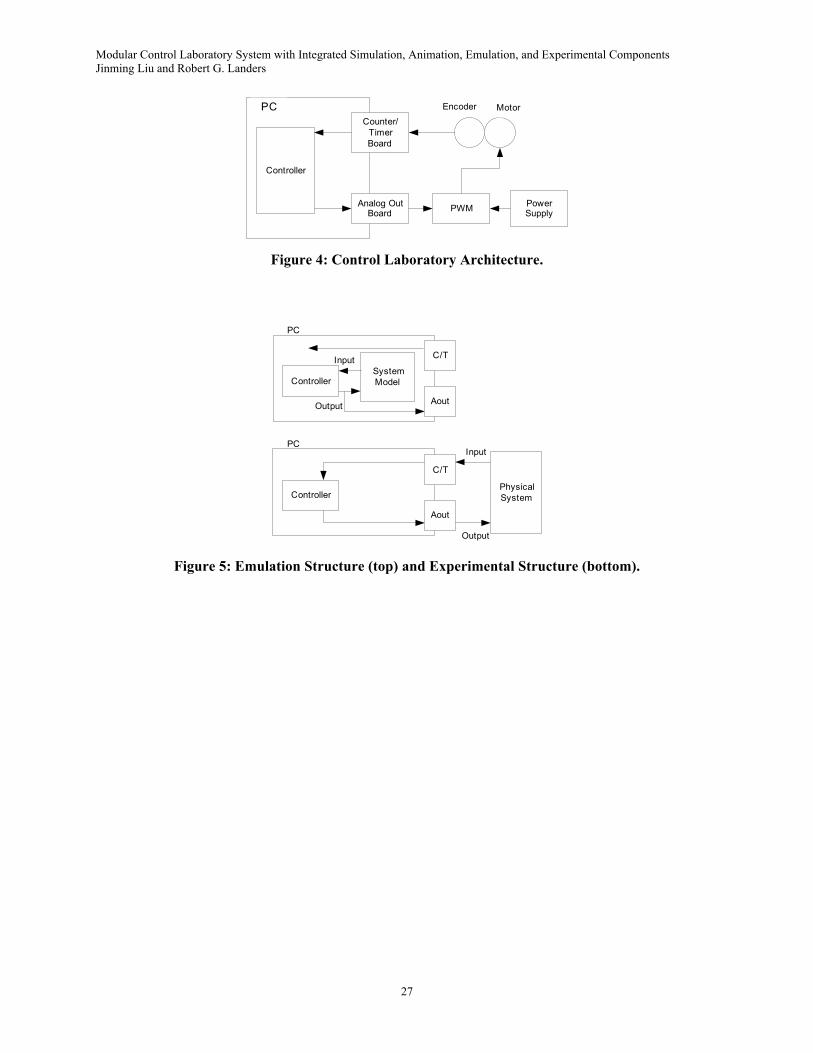
Two power supplies provide the required power for the four PWMs. Figure 4 provides a schematic

of the control laboratory system.

The architectures of the emulation and experimental programs are shown in Figure 5. The input

and output signals are transmitted, via the counter–timer and analog output boards, respectively,

between the computer and the physical system. In emulation, however, the controller receives and

sends signals to a digital system model programmed in Labview, as well as the counter/timer and


8

analog output boards, respectively. This model simulates the physical system performance while

the physical system is disconnected. Therefore, controller performance is validated on the target

processor without the possibility of damaging the physical system.

Description of Control Courses and Example Experiments

The modular control laboratory is utilized in several control courses in the Mechanical and

Aerospace Engineering and Engineering Mechanics Department at the University of Missouri at

Rolla. The courses follow a similar laboratory process. First, the students characterize the physical

system dynamics with a modeling exercise. Differential equations are generated by applying

mechanical and electrical first principles. The theoretical principles presented in the course are

utilized to design controllers. All differential equations (i.e., physical and control) are transformed

into difference equations that are numerically simulated and the results are animated. Nonlinear

effects such as quantization and saturation are included. Both simulation and animation help the

students analyze the controller performance during the design stage, and mistakes may be detected

and corrected. Controllers that are validated via simulation are then implemented in emulation

where the controller program is executed on the target processor; however, the physical system is

replaced with a digital simulation. After this step, the controllers are implemented on the physical

system. A wide variety of experiments may be designed for many different control courses, from

undergraduate to graduate.


9

In the undergraduate control course, concepts from classical control such as Routh arrays,

steady–state error, Root Locus Diagrams, proportional (P), integral (I), derivative (D), lead, and

lag control, Bode Diagrams, and Nyquist Diagrams are introduced. Linear systems and linearized

systems are considered. Several experiments are possible with the modular control laboratory

system. In a cart position tracking laboratory, one motor drives one cart and the students design a

controller to regulate the cart position for ramp inputs. This experiment allows the students to

analyze steady–state error, Root Locus Diagrams, and P controllers, and reinforces the concept of

system type. A pendulum position–tracking laboratory utilizes one motor that directly drives one

pendulum. In this laboratory, the students design a PI controller to regulate the pendulum position

at different set points. This nonlinear system reinforces the concept of linearization. In a third

laboratory, two carts, where only the first cart has a motor, are connected by a spring and the

students design a controller to regulate the position of the second cart. Frequency response, in

addition to the concepts listed above, is reinforced. Many other laboratories are possible with the

modular control laboratory system.

The introductory graduate control course at UMR concentrates on modern control methods: state

space formulation, controllability, observability, pole placement controller design, observer

design, linear quadratic regulator (LQR) controller design, and error state–space method. The

systems are more complex and multiple–input, multiple–output (MIMO) systems are introduced.

In a pendulum–balancing laboratory, a pendulum, which is free to rotate 360o, is mounted on a

cart. The objective is to move the cart to maintain the pendulum in the upward position. This


10

laboratory reinforces the concepts of stability, controllability, and observability, and different

control algorithms, such as pole placement and LQR control, and linear observers are utilized.

Moreover, the students are also required to swing up the pendulum from the downward position to

the upward position and then balance the pendulum in the upward position by moving only the

cart. In another laboratory, two carts, each of which has a motor, are connected via a spring and the

carts move along a prescribed path. This laboratory requires the use of MIMO control techniques.

The modular control laboratory can easily be reconfigured for many other graduate level

experiments. In all graduate laboratories, the students are required to estimate and reject friction

and design observers to estimate velocities.

Undergraduate and a graduate control laboratory experiments are now presented to illustrate the

utility of the modular control laboratory system developed at the University of Missouri at Rolla.

Cart Position Tracking Laboratory

The cart position tracking laboratory was designed for the undergraduate introductory controls

course. The objective of this laboratory is for the students to model, simulate, and control the

position of a cart that moves on a linear track. The reference is a ramp input where the cart moves

a distance of 90 mm at a rate of 30 mm/s and then moves a distance of 90 mm at a rate of –30 mm/s.

The motor data file is provided to the students so they can determine the motor parameters (e.g.,

mechanical inertia, electrical resistance, stall torque).


11

Ignoring the electrical dynamics of the electrical portion of the DC motor, the model of the cart

system is

a vc m

K KI VR R

ω= − (1)

x v= (2)

2 2 2m g g m g g g f g g tJ K mR v B K v K R T K R K I + = − − + (3)

where 19.7s m mg

m s s

TKT

ω ωω ω

≡ = = = , 0.00794sg

s s

T v vR mF ω ω

≡ = = = , and ( )0.0035sgnf mT ω= .

Using a Proportional controller, the control law is

[ ]c p p rV K e K x x= = − (4)

Ignoring Coulomb friction, the open–loop transfer function is

( )( ) { } { }2 2 2 2 2

a g g t

c m g g m g t v g

K K R Kx sV s R J K mR s RB K K K K s

= + + +

(5)

Combining equations (4) and (5), the closed–loop transfer function is

( )( ) tggapgvtgmggm

tggap

r KRKKKsKKKKRBsmRKJRKRKKK

sxsx

++++=

)()( 22222 (6)

Using the Final Value Theorem, the steady–state error is

atggp

gvtgmss KKRKK

KKKKRBe

22 += (7)

For a steady–state error of 0.5 mm, the controller gain is Kp = 962.2 V/m.

The closed–loop system was simulated using equations (1)–(4). Equations (2) and (3) were solved

using the Euler integration method. Note that the current was saturated at +/– 1.44 A and the


12

command voltage was saturated at +/– 10 V. An animation program was provided to the students.

After running the simulation, the reference and actual positions are input to the animation program

so the students can visualize the cart performance. The simulation results and a screen shot of the

animation are shown in Figures 6 and 7, respectively.

Before the controller was experimentally implemented, emulation was conducted to avoid

program conversion mistakes. The system model is the same for both the emulation and simulation

programs, therefore, the results are the same (see Figure 8). The experimental results are shown in

Figure 9. The desired steady–state error was not achieved due to the fact that Coulomb friction was

ignored. As a comparison, a controller with a gain of 4811 V/m, that produces a theoretical

steady–state error of 0.1 mm, was also implemented (see Figure 10). The high gain controller

causes the command voltage to constantly saturate and the system reaches an unwanted limit

cycle. The students were able to see the results and the data was emailed to them. The students

graphed the data and could also run the data through the animation file.

In this laboratory, the students utilized mathematical tools (e.g., modeling via first principles,

transfer functions, Final Value Theorem) they learned in their coursework to model the physical

system and design the controllers. The actual physical system was simulated, animated, and

emulated, and then the controller was implemented experimentally. In this way, the students were

able to go through the entire controller design cycle and understand the physical significance of the

mathematics they learned in their coursework. The integration of the simulation, animation, and


13

emulation components with the experimental portion of the laboratory provided a positive

experience for the students. The match between the simulation, emulation, and experimental

results allowed the students to gain a physical insight into the system dynamic equations. Also, the

animation was very useful in allowing students to understand the physical system and comprehend

the meaning of a ramp input. This laboratory also taught the students about real–world effects that

must be taken into account (i.e., Coulomb friction and control signal saturation). During their

coursework, students are presented with idealized linear systems. In this laboratory, the Coulomb

frictional effects, present in both the simulation and in the experiments, prevented the students

from reaching the desired steady–state error. For the large gain controller, the effects of saturation

became apparent in both the simulation and experiments.

Two Cart–One Pendulum Laboratory

A laboratory utilizing two carts and one pendulum was designed for the introductory graduate

control course. Two carts are connected with a spring and a pendulum, which is free to rotate 360o,

is mounted on one cart (cart 2). A motor and gear are assembled on the other cart (cart 1). The

objective of this laboratory is for the students to move the carts a fixed distance and then bring the

system quickly to rest. The reference position is a ramp with a slope of 0.4 m/s and an end position

of 0.5 m. Two separate coordinate systems are fixed to each cart, respectively. The reference

positions given for cart 1 and cart 2 in their own coordinate systems are the same. In addition, the

pendulum is required to remain down and should come to rest quickly (Figure 11). The students


14

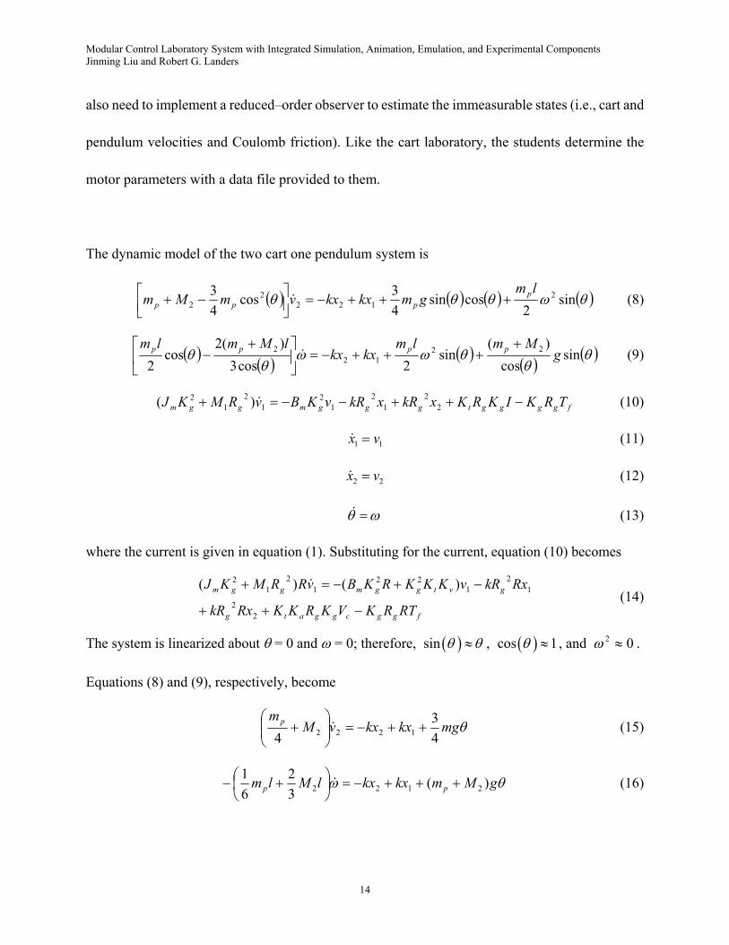
also need to implement a reduced–order observer to estimate the immeasurable states (i.e., cart and

pendulum velocities and Coulomb friction). Like the cart laboratory, the students determine the

motor parameters with a data file provided to them.

The dynamic model of the two cart one pendulum system is

( ) ( ) ( ) ( )θωθθθ sin2

cossin43cos

43 2

1222

2

lmgmkxkxvmMm p

ppp +++−=

−+ (8)

( ) ( ) ( ) ( ) ( )θθ

θωωθ

θ sincos

)(sin

2cos3)(2

cos2

2212

2 gMmlm

kxkxlMmlm pppp +

+++−=

+− (9)

fggggtgggmggm TRKIKRKxkRxkRvKBvRMKJ −++−−=+ 22

12

12

12

12 )( (10)

1 1x v= (11)

2 2x v= (12)

θ ω= (13)

where the current is given in equation (1). Substituting for the current, equation (10) becomes

fggcggatg

gvtggmggm

RTRKVKRKKRxkR

RxkRvKKKRKBvRRMKJ

−++

−+−=+

22

12

122

12

12 )()(

(14)

The system is linearized about θ = 0 and ω = 0; therefore, ( )sin θ θ≈ , ( )cos 1θ ≈ , and 02 ≈ω .

Equations (8) and (9), respectively, become

θmgkxkxvMmp

43

4 1222 ++−=

+ (15)

θω gMmkxkxlMlm pp )(32

61

2122 +++−=

+− (16)


15

In order to use state feedback control to drive the errors to zero, the system states are redefined as

1e , 1v , 2e , 2v , θ, and ω, where iri xxe −= (i = 1, 2), and xr is the same for both carts in their

respective coordinate systems. Rearranging, iri exx −= (i = 1, 2) and iri exx −= (i = 1, 2). Note

that rx is a ramp input, thus, 0≠rx . Substituting iri exx −= (i = 1, 2) into equations (14)–(16)

( ) ( )2 2 2 2 21 1 1 1 2m g g m t v g g g t a g g c g g fJ K M R Rv B R K K K v kRR e kRR e K K R K V K R RT+ = − + + − + − (17)

θgmkekevMm

pp

43

4 1222 +−=

+ (18)

θω gMmkekelMlm pp )(32

61

2122 ++−=

+− (19)

Note the terms with xr are canceled. A control algorithm for exogenous signals (i.e., references and

disturbances) is applied [Friedland, 1986]. The state space description is cz Az BV= + and y = Cz,

where z, A, B, and C, respectively, are

1

2

1

2

r

f

ee

xz

vv

T

θ

ω

=

0 0 0 1 1 0 0 00 0 0 1 0 1 0 00 0 0 0 0 0 1 00 0 0 0 0 0 0 0

253 253 0 43.4 0 0 0 242773 772 0.42 0 0 0 0 0

2040 2040 27.1 0 0 0 0 00 0 0 0 0 0 0 0

A

− − = − − − −

− −

0000

2.65000

B

=

(20)

1 0 0 0 0 0 0 00 1 0 0 0 0 0 00 0 1 0 0 0 0 00 0 0 1 0 0 0 0

C

=

(21)

An LQR controller is designed. The control law is given by

cV Gz= − (22)

The weighting matrices, selected via trial and error, are


16

[ ]5000 1 5000 1 2000 1 1 1 1Q diag R= = (23)

The Matlab function lqr is used to calculate the gain matrix

[ ]292.86 5.76 192.86 13.20 39.85 4.04 35.35 91.29G = − − − − (24)

The closed–loop pole locations are located at 0, 0, –7.6, –38.9, –1.8±4i, and –4.3±30i.

The pendulum and cart positions are measured via three separate encoders and the reference

position is predefined; thus, e1, e2, θ, and rx are measurable. The other states, namely, v1, v2, ω,

and Tf, must be estimated. As a result, a reduced order observer is designed. The unmeasurable

states are estimated by pLyz +=2ˆ , where p is described by

cHVyCALCAzFp +−+= −11111212 )(ˆ (25)

where 2 1 2ˆˆ ˆ ˆˆ

T

fz v v Tω = , 12122 ALCAF −= , 112 BLCBH −= , and the matrices 11A , 12A ,

21A , 22A , 1B , 2B , and 1C (i.e., the corresponding sub–matrices of A, B, and C) are

=

0000000010001000

11A

12

1 0 0 00 1 0 00 0 1 00 0 0 242

A

− − = −

21

253 253 0 0773 773 0.42 0

2040 2040 27.1 00 0 0 0

A

− − = − −

22

43.4 0 0 2420 0 0 00 0 0 00 0 0 0

A

− − =

=

0000

1B

=

00065.2

2B

=

1000010000100001

1C (26)

The desired observer closed–loop pole locations, selected by trial and error, are –6, –6.5, –7, and

–7.5. The Matlab function place is used to calculate the observer gain matrix

28.9 0 0 00 -6 0 00 0 6.5 0

0.22 0 0 0

L

=

(27)


17

When applying the observer to the system, 1v , 2v , ω, and Tf are estimated and the control law

becomes

1 2 1 2ˆˆ ˆ ˆˆ

T

c r fV Gz G e e x v v Tθ ω = − = − (28)

Equation (1), where ωm has been replaced by Kg*v/Rg, and equations (8)–(13) are used to simulate

the closed–loop nonlinear system. The differential equations were solved using a 4th order

Runge–Kutta integration routine. Again, the command voltage was saturated between +/– 10 V

and the current is saturated between +/– 1.44 A. An animation program was developed to provide

the students a means to visualize the system performance given simulation, emulation, or

experimental data. The simulation results are shown in Figure 12, and Figure 13 is a screen shot of

the animation.

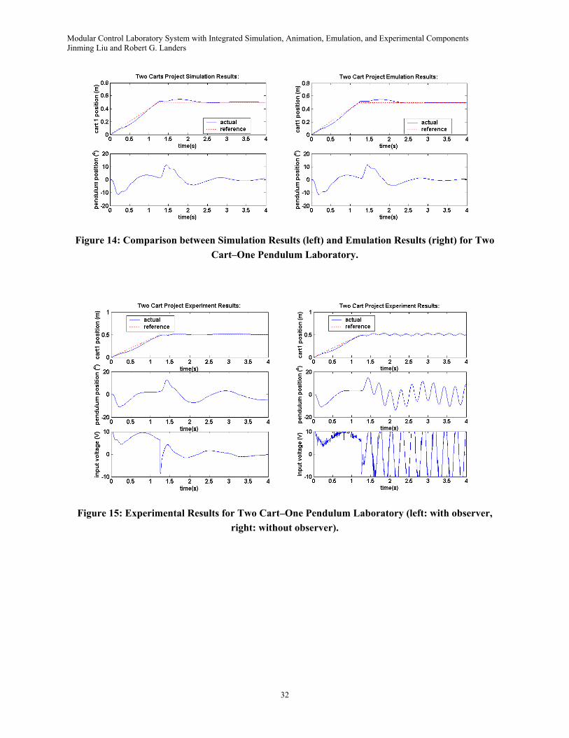
Similar to the cart position project, the controller is implemented in emulation before it is

implemented experimentally. The result is shown in Figure 14. Because both simulation and

emulation use the same system model and the same sample period, the results are identical and,

thus, the controller is verified on the target processor. Next, both the controller and the

reduced–order observer are experimentally implemented on the physical system. The results are

shown in Figure 15 (left) for the experiment with a reduced–order observer. Figure 15 (right)

presents the experimental results when using the same controller where the velocities are estimated

by first order backward difference equations. When the observer was not utilized, the encoder

quantization drove the closed–loop system unstable.


18

In this laboratory, the students utilized mathematical tools and techniques (e.g., state–space

formulation, lqr control, reduced order observer design) they learned in their coursework to model

the physical system and design the controller and observer. This laboratory, as compared to the

cart position tracking laboratory, provides the students with an opportunity to investigate a more

complex physical system using more sophisticated control techniques. The students were required

to linearize the system and they utilized exogenous control techniques, LQR control algorithms,

and observers. Again, the students go through the entire controller design cycle and can understand

the physical significance of the mathematics they learned in their coursework. The students also

learned how encoder quantization can adversely affect velocity estimation and, hence, closed–loop

system performance.

Summary and Conclusions

In this paper, simulation, animation, emulation, and experimental components were integrated to

create a modular control laboratory system. The physical components were designed such that a

wide variety of laboratory setups may be easily constructed that are suitable for control courses,

from undergraduate to graduate. Two laboratories were presented. The animation component

augmented the simulations to provide an increased understanding of the course material. The

animation was particularly useful in the early control design stage as it allowed for visual analysis.

The emulation component eliminated mistakes encountered when uploading control programs to


19

the target processor. These laboratories also introduced the students to real–world effects that, if

not taken into account, can significantly degrade controller performance.

References

Amira Measuring and Control Technology, 2003, http://www.amira.de/.

Anderson, M.J. and Grantham, W.J., 1989, “Lyapunov Optimal Feedback Control of a

Nonlinear Inverted Pendulum,” ASME Journal of Dynamic Systems, Measurement, and Control,

Vol. 111, pp. 554–558.

Astrom, K.J. and Furuta, K., 1996, “Swinging Up a Pendulum by Energy Control,” 13th

Triennial World Congress of IFAC, San Francisco, California, June 30 – July 5, pp. 37–42.

Brusic, S.A. and Laporte, J.E., 1999, “The Status of Modular Technology Education in

Virginia,” International Technology Education Association Conference, Indianapolis, Indiana,

March 28–30.

Chapuis, J., Eck, C., and Geering, H.P., 1997, “Autonomously Flying Helicopter,” 4th IFAC

Symposium on Control Education, Istanbul, Turkey, July 14–16, pp. 119–124.

Cheok, K.C. and Kheir, N.A., 1993, “A Computer Visualizaiton Teachware for Evaluating the

Performance of Control System,” American Control Conference, San Francisco, California, June

2–4, pp. 1244–1245.

Clement, W.I. and Knowles, K.A., 1994, “An Instructional Robotics and Machine Vision

Laboratory,” IEEE Transactions on Education, Vol. 37, No. 1, pp. 87–90.


20

Cipriano, A., Saez, D., and Ramos, M., 1995, “Fuzzy Control on a Laboratory Environment,”

Industrial Electronics, Vol. 2, pp. 500–505.

Dixon, W.E., Dawson, D.M., Costic, B.T., and De Queiroz, M.S., 2002, “A MATLAB–based

Control Systems Laboratory Experience for Undergraduate Students: Toward Standardization and

Shared Resources,” IEEE Transactions on Education, Vol. 45, No. 3, pp. 218–226.

Friedland, B., 1986, Control System Design, McGraw Hill, New York.

Furuta, K., Xu, Y., and Gabasov, R., 1999, “Computation of Time Optimal Swing Up Control

of Single Pendulum,” Industrial Electronics Society, IECON '99 Proceedings, Vol. 3, pp. 1165

–1170.

Hagan, M.T. and Latino, C.D., 1995, “A Modular Control Systems Laboratory,” Computer

Applications in Engineering Education, Vol. 3, No. 2, pp. 89–96.

Horacek, P., 2000, “Laboratory Experiments for Control Theory Courses: a Survey,” Annual

Reviews in Control, Vol. 24, pp. 151–162.

Kawashima, T., 1998, “Swing–up and Stabilization of Inverted Pendulum Using Only One

Sliding Mode Controller with Nonlinear Model Observer,” 4th International Conference on

Motion and Vibration Control, Zurich, Switzerland, August 25–29, Vol. 1, pp. 97–102.

Kheir, N.A., Astrom, K.J., Auslander, D., Cheok, K.C., Franklin, G.F., Masten, M., and

Rabins, M., 1996, “Control System Engineering Education,” Automatica, Vol. 32, No. 2, pp.

147–166.


21

Ko, C.C., Chen, B.M., Chen, J., Zhuang, Y., and Tan, K.C., 2001, “Development of a

Web–based Laboratory for Control Experiments on a Coupled Tank Apparatus,” IEEE

Transactions on Education, Vol. 44, No. 1, pp. 76–86.

Magana, M.E. and Holzapfel, F., 1998, “Fuzzy–logic Control of an Inverted Pendulum with

Vision Feedback,” IEEE Transactions on Education, Vol. 41, No. 2, pp. 165–170.

Malmborg, J. and Eker, J., 1997, “Hybrid Control of a Double Tank System,” IEEE

Conference on Control Applications, Hartford, Connecticut, October 5–7, pp. 137–138.

Meier, H., Farwig, Z., and Unbehauen, H., 1990, “Discrete Computer Control of a Triple

Inverted Pendulum,” Optimal Control Applications and Methods, Vol. 11, pp. 157–171.

Mori, S., Nishinara, H., and Furuta, K., 1976, “Control of Unstable Mechanical System,

Control of Pendulum,” International Journal of Control, Vol. 23, pp. 673–692.

Nakano, K., Kondou, T., Yamaguchi, Y., Matsuo, T., and Choshi, H., 1996, “Robust

Stabilization of an Inverted Pendulum System Via Rule–based Sliding–mode Generation,” 13th

Triennial World Congress of IFAC, San Francisco, California, June 30 – July 5, Vol. F, pp.

223–228.

Overstreet, J.W. and Tzes, A., 1999, “Internet–based Real–time Control Engineering

Laboratory,” IEEE Control Systems Magazine, Vol. 19, No. 5, pp. 19–34.

Sasaki, N., Ohyama, Y., and Ikebe, J., 1997, “Design Exercises for Robust Controller Using a

Double Inverted Pendulum,” 4th IFAC Symposium on Control Education, Istanbul, Turkey, July

14–16, pp. 301–305.


22

Sridharan, S. and Sridharan, G., 2002, “Ball on Beam on Roller: a New Control Laboratory

Device,” Industrial Electronics, Vol. 4, pp. 1318–1321.

Swamy, N., Kuljaca, O., and Lewis, F.L., 2002, “Internet–based Educational Control Systems

Lab Using NetMeeting,” IEEE Transactions on Education, Vol. 45, No. 2, pp. 145–151.

Whelan, J. and Ringwood, J.V., 1994, “A Demonstration Rig For Control Systems Based On

the Ball and Beam with Vision Feedback,” 3rd IFAC Symposium on Control Education, Tokyo,

Japan, August 1–2, pp. 9–15.

Yamakita, M., Iwashiro, M., Sugahara, Y., and Furuta, K., 1995, “Robust Swing Up Control

of a Double Pendulum,” American Control Conference, Seattle, Washington, June 21–23, pp.

290–295.

Yi, J., Yubazaki, N., and Hirota, K., 1999, “Upswing and Stabilization Control of Inverted

Pendulum and Cart System by the SIRMs Dynamically Connected Fuzzy Inference Model,” IEEE

International Fuzzy Systems Conference, Seoul, Korea, August 22–25, Vol. 1, pp. 400–405.

Zhao, Z., Linton, J., and Kanellakopoulos, I., 2000, “SMARTREV: A Control Laboratory on

Wheels,” American Control Conference, Chicago, Illinois, June 28–30, pp. 559–563.

NOMENCLATURE

an : Normal acceleration (m/s2)

at : Tangential acceleration (m/s2)

Bm : Motor viscous damping (Nms)


23

ess : Steady state position error (m)

F : Driving force from motor on cart (N)

Fx : Reaction force in x–direction between cart and pendulum (N)

Fy : Reaction force in y–direction between cart and pendulum (N)

k : Spring force constant (N/m)

Ka : PWM gain

Kg : Motor internal gearbox gain

Kp : Proportional controller gain (V/m)

Kt : Torque constant [Nm/A]

Kv : Voltage constant [V/(rad/s)]

I : Motor current (A)

Jm : Motor inertia (kgm2)

l : Pendulum length (m)

m : Cart mass (kg)

mp : Pendulum mass (kg)

M1 : Cart 1 mass (kg)

M2 : Cart 2 mass (kg)

R : Motor electrical resistance (Ohms)

Rg : Motor gear radius (m)

Tf : Coulomb friction torque (Nm)

Tm : Torque drained from motor (Nm)


24

Ts : Torque applied to shaft (Nm)

v : Cart velocity (m/s)

v1 : Cart 1 velocity (m/s)

v2 : Cart 2 velocity (m/s)

x : Cart position (m)

x1 : Cart 1 position (m)

x2 : Cart 2 position (m)

xr : Reference cart position (m)

θ : Pendulum angular position (rad)

ω : Pendulum angular velocity (rad/s)

ωm : Motor angular velocity (rad/s)

ωs : Shaft angular velocity (rad/s)


25

PowerSupply PWM

Motor

CartLinearTrack

Encoder

Figure 1: Modular Control Laboratory (top view).

Motor

Encoder

Pendulum

Cart Pendulum

Encoders

Motors

Spring

Cart

Figure 2: Two Configurations of the Modular Control Laboratory: SISO cart and pendulum (left), and MIMO cart and pendulum (right).


26

Figure 3: Two Cart–One Pendulum Laboratory Graphical User Interface (top) and Icon–Based Sensing and Control Program (bottom).


27

Controller

Analog OutBoard

Counter/TimerBoard

PWM PowerSupply

PC Encoder Motor

Figure 4: Control Laboratory Architecture.

PC

PC

Output

Input

Output

Input

SystemModel

PhysicalSystemController

Controller

C/T

Aout

C/T

Aout

Figure 5: Emulation Structure (top) and Experimental Structure (bottom).


28

Figure 6: Cart Position Tracking Laboratory Simulation Results.

Figure 7: Cart Position Tracking Laboratory Animation Screenshot with Actual (dot in cart center) and Reference (dot to the right of cart) Positions.


29

Figure 8: Comparison between Simulation Results (left) and Emulation Results (right) for Cart Position Tracking Laboratory.

Figure 9: Cart Position Tracking Laboratory Experimental Results (Kp = 962.2 V/m).


30

Figure 10: Cart Position Tracking Laboratory Experimental Results (Kp = 4811 V/m).

θ

x1 x2 xr

M

Figure 11: Two Cart–One Pendulum Laboratory Schematic.


31

Figure 12: Two Cart–One Pendulum Laboratory Simulation Results.

Figure 13: Two Cart–One Pendulum Laboratory Animation Screenshot.


32

Figure 14: Comparison between Simulation Results (left) and Emulation Results (right) for Two Cart–One Pendulum Laboratory.

Figure 15: Experimental Results for Two Cart–One Pendulum Laboratory (left: with observer,

right: without observer).

Modular Control Laboratory System with Integrated ...

Documents

Transcript of Modular Control Laboratory System with Integrated ...