Modèles macroscopiques de trafic routier et piétonnier · Introduction Phase transition Flux...
72
Introduction Phase transition Flux constraints Pedestrians Conclusion Congrès SMAI 2013 Modèles macroscopiques de trafic routier et piétonnier Paola Goatin EPI OPALE INRIA Sophia Antipolis - Méditerranée [email protected] Seignosse Le Penon, 30 mai, 2013
Transcript of Modèles macroscopiques de trafic routier et piétonnier · Introduction Phase transition Flux...
Introduction Phase transition Flux constraints Pedestrians Conclusion
Congrès SMAI 2013
Modèles macroscopiques de trafic routier et piétonnier
Paola Goatin
EPI OPALE
INRIA Sophia Antipolis - Méditerranée
Seignosse Le Penon, 30 mai, 2013

Introduction Phase transition Flux constraints Pedestrians Conclusion
Outline of the talk
1 Traffic flow models
2 Phase transition models
3 Flux constraints
4 Crowd dynamics
5 Conclusion
P. Goatin (INRIA) Modèles macroscopiques de trafic routier et piétonnier 30 mai, 2013 2 / 50

Introduction Phase transition Flux constraints Pedestrians Conclusion
Traffic flow models
Three possible scales:
Microscopic:ODEs systemnumerical simulationsmany parameters
Kinetic:distribution function of the microscopic statesBoltzmann-like equations
Macroscopic:PDEs from fluid dynamicsanalytical theoryfew parameterssuitable to formulate control and optimization problems
P. Goatin (INRIA) Modèles macroscopiques de trafic routier et piétonnier 30 mai, 2013 3 / 50
Introduction Phase transition Flux constraints Pedestrians Conclusion
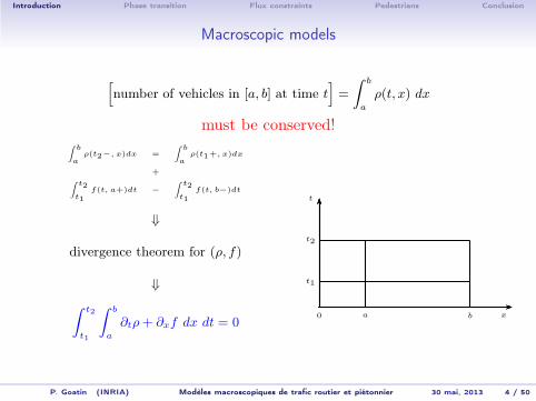
Macroscopic models
[
number of vehicles in [a, b] at time t]
=
∫ b
a
ρ(t, x) dx
must be conserved!
∫b
aρ(t2−, x)dx =
∫b
aρ(t1+, x)dx
+∫ t2
t1
f(t, a+)dt −
∫ t2
t1
f(t, b−)dt
⇓
divergence theorem for (ρ, f)
⇓
∫ t2
t1
∫ b
a
∂tρ+ ∂xf dx dt = 0x
t
t1
t2
0 a b
P. Goatin (INRIA) Modèles macroscopiques de trafic routier et piétonnier 30 mai, 2013 4 / 50

Introduction Phase transition Flux constraints Pedestrians Conclusion
Conservation laws
(System of) PDEs of the form
∂tu(t,x) + divxf(u(t,x)) = 0 t > 0, x ∈ IRD
where u ∈ IRn conserved quantitiesf : IRn×D → IR smooth strictly hyperbolic flux
Basic facts:
No classical smooth solutions =⇒ weak solutions
No uniqueness =⇒ entropy conditions
Well posedness known only if minn,D = 1
P. Goatin (INRIA) Modèles macroscopiques de trafic routier et piétonnier 30 mai, 2013 5 / 50

Introduction Phase transition Flux constraints Pedestrians Conclusion
Requirements
No information propagates faster than vehicles (anisotropy)
Flux-density relation: f(t, x) = ρ(t, x)v(t, x).
Density and mean velocity must be non-negative and bounded:0 ≤ ρ(t, x), v(t, x) < +∞, ∀x, t > 0.
Different from fluid dynamics:preferred directionno conservation of momentum / energyno viscosityAvogadro number for vehicles: 106 vh/lane×km ≪ 6 · 1023
P. Goatin (INRIA) Modèles macroscopiques de trafic routier et piétonnier 30 mai, 2013 6 / 50

Introduction Phase transition Flux constraints Pedestrians Conclusion
Macroscopic models
n≪ 6 · 1023 but ...
P. Goatin (INRIA) Modèles macroscopiques de trafic routier et piétonnier 30 mai, 2013 7 / 50

Introduction Phase transition Flux constraints Pedestrians Conclusion
First order models
Lighthill-Whitham ’55, Richards ’56, Greenshields ’35:
Non-linear transport equation: scalar conservation law
∂tρ+ ∂xf(ρ) = 0, f(ρ) = ρv(ρ)
Empirical flux function: fundamental diagram
with R the maximal or jam density and ρc the critical density:
flux is increasing for ρ ≤ ρc: free-flow phase
flux is decreasing for ρ ≥ ρc: congestion phase
P. Goatin (INRIA) Modèles macroscopiques de trafic routier et piétonnier 30 mai, 2013 8 / 50
Ωf
Ωc
R ρ
f
0 ρcNewell-Daganzo
Ωf Ωc
R ρ
f
0 ρcGreenshields

Introduction Phase transition Flux constraints Pedestrians Conclusion
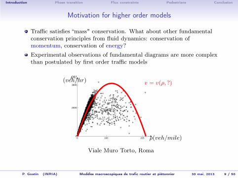
Motivation for higher order models
Traffic satisfies “mass" conservation. What about other fundamentalconservation principles from fluid dynamics: conservation ofmomentum, conservation of energy?
Experimental observations of fundamental diagrams are more complexthan postulated by first order traffic models
P. Goatin (INRIA) Modèles macroscopiques de trafic routier et piétonnier 30 mai, 2013 9 / 50
0 100 2250
2000
3600
ρ(veh/mile)
ρv(veh/hr)
Viale Muro Torto, Roma
Introduction Phase transition Flux constraints Pedestrians Conclusion
Motivation for higher order models
Traffic satisfies “mass" conservation. What about other fundamentalconservation principles from fluid dynamics: conservation ofmomentum, conservation of energy?
Experimental observations of fundamental diagrams are more complexthan postulated by first order traffic models
P. Goatin (INRIA) Modèles macroscopiques de trafic routier et piétonnier 30 mai, 2013 9 / 50
0 100 2250
2000
3600
ρ(veh/mile)
ρv(veh/hr) v = v(ρ, ?)
Viale Muro Torto, Roma

Introduction Phase transition Flux constraints Pedestrians Conclusion
Motivation for higher order models
Traffic satisfies “mass" conservation. What about other fundamentalconservation principles from fluid dynamics: conservation ofmomentum, conservation of energy?
Experimental observations of fundamental diagrams are more complexthan postulated by first order traffic models
P. Goatin (INRIA) Modèles macroscopiques de trafic routier et piétonnier 30 mai, 2013 9 / 50
0 100 2250
2000
3600
ρ(veh/mile)
ρv(veh/hr)
fluid flow
v = vf (ρ)
congestion
v = vc(ρ, ?)
Viale Muro Torto, Roma

Introduction Phase transition Flux constraints Pedestrians Conclusion
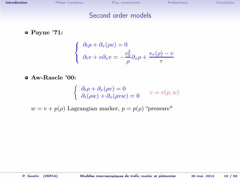
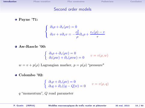
Second order models
Payne ’71:
∂tρ+ ∂x(ρv) = 0
∂tv + v∂xv = −c20ρ∂xρ+
v∗(ρ)− v
τ
Critics (Del Castillo et al. ’94, Daganzo ’95):drivers should have only positive speeds;anisotropy: drivers should react only to stimuli from the front.
P. Goatin (INRIA) Modèles macroscopiques de trafic routier et piétonnier 30 mai, 2013 10 / 50
Introduction Phase transition Flux constraints Pedestrians Conclusion
Second order models
Payne ’71:
∂tρ+ ∂x(ρv) = 0
∂tv + v∂xv = −c20ρ∂xρ+
v∗(ρ)− v
τ
Aw-Rascle ’00:∂tρ+ ∂x(ρv) = 0∂t(ρw) + ∂x(ρvw) = 0
v = v(ρ,w)
w = v + p(ρ) Lagrangian marker, p = p(ρ) “pressure"
Colombo ’02:∂tρ+ ∂x(ρv) = 0∂tq + ∂x((q −Q)v) = 0
v = v(ρ, q)
q “momentum”, Q road parameter
P. Goatin (INRIA) Modèles macroscopiques de trafic routier et piétonnier 30 mai, 2013 10 / 50

Introduction Phase transition Flux constraints Pedestrians Conclusion
Outline of the talk
1 Traffic flow models
2 Phase transition models
3 Flux constraints
4 Crowd dynamics
5 Conclusion
P. Goatin (INRIA) Modèles macroscopiques de trafic routier et piétonnier 30 mai, 2013 11 / 50

Introduction Phase transition Flux constraints Pedestrians Conclusion
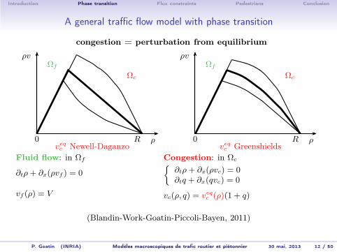
A general traffic flow model with phase transition
Fluid flow: in Ωf
∂tρ+ ∂x(ρvf ) = 0
vf (ρ) = V
Congestion: in Ωc∂tρ+ ∂x(ρvc) = 0
vc(ρ, q) = veqc (ρ)
(Blandin-Work-Goatin-Piccoli-Bayen, 2011)
P. Goatin (INRIA) Modèles macroscopiques de trafic routier et piétonnier 30 mai, 2013 12 / 50
congestion = perturbation from equilibrium
Ωf
Ωc
R ρ
ρv
0veqc Newell-Daganzo
Ωf
Ωc
R ρ
ρv
0veqc Greenshields
Introduction Phase transition Flux constraints Pedestrians Conclusion
A general traffic flow model with phase transition
Fluid flow: in Ωf
∂tρ+ ∂x(ρvf ) = 0
vf (ρ) = V
Congestion: in Ωc∂tρ+ ∂x(ρvc) = 0∂tq + ∂x(qvc) = 0
vc(ρ, q) = veqc (ρ)(1 + q)
(Blandin-Work-Goatin-Piccoli-Bayen, 2011)
P. Goatin (INRIA) Modèles macroscopiques de trafic routier et piétonnier 30 mai, 2013 12 / 50
congestion = perturbation from equilibrium
Ωf
Ωc
R ρ
ρv
0veqc Newell-Daganzo
Ωf
Ωc
R ρ
ρv
0veqc Greenshields

Introduction Phase transition Flux constraints Pedestrians Conclusion
Analytical study
Analysis of congestion phase:
Eigenvalues λ1(ρ, q) = veqc (ρ) (1 + q) +q veqc (ρ) + ρ (1 + q)∂ρ veqc (ρ)
λ2(ρ, q) = veqc (ρ)(1 + q)
Eigenvectors r1 =
(
ρq
)
r2 =
(
veqc (ρ)−(1 + q) ∂ρ veqc (ρ)
)
Nature of theLax-curves
∇λ1.r1 = ρ2 (1 + q)∂2ρρ veqc (ρ) +
2 ρ (1+2 q) ∂ρ veqc (ρ)+2 q veqc (ρ)
∇λ2.r2 = 0
Riemann in-variants
veqc (ρ) (1 + q) q/ρ
Across first family waves (shocks or rarefactions) ρ/q is conserved,which models the average driver aggressiveness
Across second family waves (contact discontinuities) v is conserved(like in free flow)
P. Goatin (INRIA) Modèles macroscopiques de trafic routier et piétonnier 30 mai, 2013 13 / 50
Introduction Phase transition Flux constraints Pedestrians Conclusion
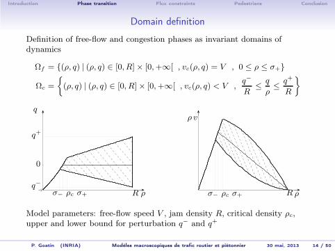
Domain definition
Definition of free-flow and congestion phases as invariant domains ofdynamics
Ωf = (ρ, q) | (ρ, q) ∈ [0, R]× [0,+∞[ , vc(ρ, q) = V , 0 ≤ ρ ≤ σ+
Ωc =
(ρ, q) | (ρ, q) ∈ [0, R]× [0,+∞[ , vc(ρ, q) < V ,q−
R≤q
ρ≤q+
R
−1 σ− ρc σ+ ρ
0
q
R
q+
q−
σ− ρc σ+ R ρ
ρ v
Model parameters: free-flow speed V , jam density R, critical density ρc,upper and lower bound for perturbation q− and q+
P. Goatin (INRIA) Modèles macroscopiques de trafic routier et piétonnier 30 mai, 2013 14 / 50

Introduction Phase transition Flux constraints Pedestrians Conclusion
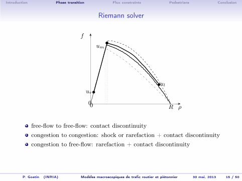
Riemann solver
free-flow to free-flow: contact discontinuity
P. Goatin (INRIA) Modèles macroscopiques de trafic routier et piétonnier 30 mai, 2013 15 / 50
R ρ
f
00
ul
ur

Introduction Phase transition Flux constraints Pedestrians Conclusion
Riemann solver
free-flow to free-flow: contact discontinuity
congestion to congestion: shock or rarefaction + contact discontinuity
P. Goatin (INRIA) Modèles macroscopiques de trafic routier et piétonnier 30 mai, 2013 15 / 50
R ρ
f
00
ul
um
ur
Introduction Phase transition Flux constraints Pedestrians Conclusion
Riemann solver
free-flow to free-flow: contact discontinuity
congestion to congestion: shock or rarefaction + contact discontinuity
congestion to free-flow: rarefaction + contact discontinuity
P. Goatin (INRIA) Modèles macroscopiques de trafic routier et piétonnier 30 mai, 2013 15 / 50
R ρ
f
00
um
ul
ur

Introduction Phase transition Flux constraints Pedestrians Conclusion
Riemann solver
free-flow to free-flow: contact discontinuity
congestion to congestion: shock or rarefaction + contact discontinuity
congestion to free-flow: rarefaction + contact discontinuity
free-flow to congestion: phase transition + contact discontinuity
P. Goatin (INRIA) Modèles macroscopiques de trafic routier et piétonnier 30 mai, 2013 15 / 50
R ρ
f
00
um
ur
ul

Introduction Phase transition Flux constraints Pedestrians Conclusion
Mass conservation across phase transitions
Phase transition speed Λ must satisfy Rankine-Hugoniot conditions
Λ(ρ+ − ρ−) = F+ − F−
with
F− =
ρ− vf (ρ−) if ρ− ∈ Ωf
ρ− vc(ρ−, q−) if ρ− ∈ Ωc
F+ =
ρ+ vf (ρ+) if ρ+ ∈ Ωf
ρ+ vc(ρ+, q+) if ρ+ ∈ Ωc
P. Goatin (INRIA) Modèles macroscopiques de trafic routier et piétonnier 30 mai, 2013 16 / 50

Introduction Phase transition Flux constraints Pedestrians Conclusion
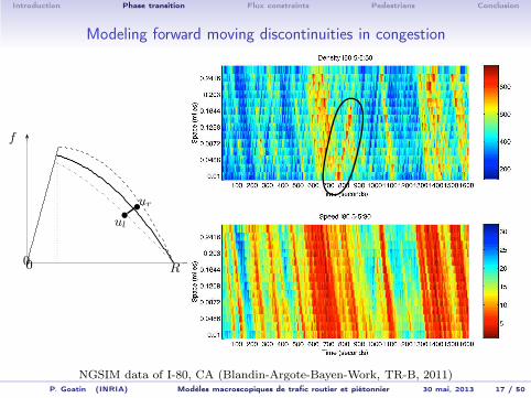
Modeling forward moving discontinuities in congestion
NGSIM data of I-80, CA (Blandin-Argote-Bayen-Work, TR-B, 2011)P. Goatin (INRIA) Modèles macroscopiques de trafic routier et piétonnier 30 mai, 2013 17 / 50
R ρ
f
00
ul
ur
Introduction Phase transition Flux constraints Pedestrians Conclusion
Modeling forward moving discontinuities in congestion
NGSIM data of I-80, CA (Blandin-Argote-Bayen-Work, TR-B, 2011)P. Goatin (INRIA) Modèles macroscopiques de trafic routier et piétonnier 30 mai, 2013 17 / 50
R ρ
f
00
ul
ur
Introduction Phase transition Flux constraints Pedestrians Conclusion
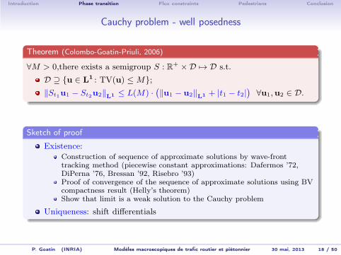
Cauchy problem - well posedness
Theorem (Colombo-Goatin-Priuli, 2006)
∀M > 0,there exists a semigroup S : R+ ×D 7→ D s.t.
D ⊇ u ∈ L1 : TV(u) ≤ M;
‖St1u1 − St2u2‖L1 ≤ L(M) ·(‖u1 − u2‖L1 + |t1 − t2|
)∀u1,u2 ∈ D.
Sketch of proof
Existence:Construction of sequence of approximate solutions by wave-fronttracking method (piecewise constant approximations: Dafermos ’72,DiPerna ’76, Bressan ’92, Risebro ’93)Proof of convergence of the sequence of approximate solutions using BVcompactness result (Helly’s theorem)Show that limit is a weak solution to the Cauchy problem
Uniqueness: shift differentials
P. Goatin (INRIA) Modèles macroscopiques de trafic routier et piétonnier 30 mai, 2013 18 / 50
Introduction Phase transition Flux constraints Pedestrians Conclusion
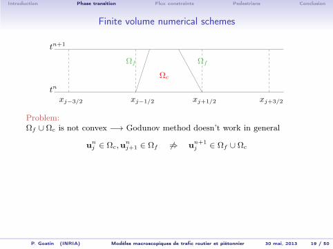
Finite volume numerical schemes
tn+1
tn
xj−3/2 xj−1/2 xj+1/2 xj+3/2
Ωf Ωf
Ωc
Problem:Ωf ∪ Ωc is not convex −→ Godunov method doesn’t work in general
unj ∈ Ωc,u
nj+1 ∈ Ωf 6⇒ u
n+1j ∈ Ωf ∪ Ωc
P. Goatin (INRIA) Modèles macroscopiques de trafic routier et piétonnier 30 mai, 2013 19 / 50

Introduction Phase transition Flux constraints Pedestrians Conclusion
Finite volume numerical schemes
tn+1
tn
xj−3/2 xj−1/2 xj+1/2 xj+3/2
Ωf Ωf
Ωc
Problem:Ωf ∪ Ωc is not convex −→ Godunov method doesn’t work in general
unj ∈ Ωc,u
nj+1 ∈ Ωf 6⇒ u
n+1j ∈ Ωf ∪ Ωc
Solutions
moving meshes for phase transitions:
Zhong - Hou - LeFloch ’96;
transport-equilibrium method: Chalons ’07.
P. Goatin (INRIA) Modèles macroscopiques de trafic routier et piétonnier 30 mai, 2013 19 / 50

Introduction Phase transition Flux constraints Pedestrians Conclusion
Godunov method
tn+1
tn
xj−3/2 xj−1/2 xj+1/2 xj+3/2
Ωf Ωf
Ωc
un+1j =
1
∆x
∫ xj+1/2
xj−1/2
v(∆t, x)dx
P. Goatin (INRIA) Modèles macroscopiques de trafic routier et piétonnier 30 mai, 2013 20 / 50

Introduction Phase transition Flux constraints Pedestrians Conclusion
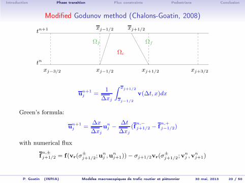
Modified Godunov method (Chalons-Goatin, 2008)
tn+1
tn
xj−3/2 xj−1/2 xj+1/2 xj+3/2
xj−1/2 xj+1/2
Ωf Ωf
Ωc
un+1j =
1
∆xj
∫ xj+1/2
xj−1/2
v(∆t, x)dx
P. Goatin (INRIA) Modèles macroscopiques de trafic routier et piétonnier 30 mai, 2013 20 / 50
Introduction Phase transition Flux constraints Pedestrians Conclusion
Modified Godunov method (Chalons-Goatin, 2008)
tn+1
tn
xj−3/2 xj−1/2 xj+1/2 xj+3/2
xj−1/2 xj+1/2
Ωf Ωf
Ωc
un+1j =
1
∆xj
∫ xj+1/2
xj−1/2
v(∆t, x)dx
Green’s formula:
un+1j =
∆x
∆xjunj −
∆t
∆xj
(fn,−j+1/2 − f
n,+j−1/2)
with numerical flux
fn,±j+1/2 = f(vr(σ
±j+1/2;u
nj ,u
nj+1))− σj+1/2vr(σ
±j+1/2;v
nj ,v
nj+1)
P. Goatin (INRIA) Modèles macroscopiques de trafic routier et piétonnier 30 mai, 2013 20 / 50

Introduction Phase transition Flux constraints Pedestrians Conclusion
Random sampling
tn+1
tn
xj−3/2 xj−1/2 xj+1/2 xj+3/2
un+1j−1 u
n+1j u
n+1j+1
Ωf Ωf
Ωc
(an) equi-distributed random sequence in ]0, 1[ (ex. Van der Corput)
un+1j =
un+1j−1 si an+1 ∈ ]0, ∆t
∆xσ+j−1/2[
un+1j si an+1 ∈ [ ∆t
∆xσ+j−1/2, 1 +
∆t∆xσ−j+1/2[
un+1j+1 si an+1 ∈ [1 + ∆t
∆xσ−j+1/2
, 1[
σj+1/2 = phase transition speed at xj+1/2
σ+j+1/2 = maxσj+1/2, 0, σ
−j+1/2 = minσj+1/2, 0
P. Goatin (INRIA) Modèles macroscopiques de trafic routier et piétonnier 30 mai, 2013 21 / 50

Introduction Phase transition Flux constraints Pedestrians Conclusion
Benchmark test
Newell-Daganzo with V = 45, R = 1000, ρc = 220, σ− = 190, σ+ = 270:
−0.5 0 0.50
100
200
300
400
500
600
700
800
900
1000
ρ
Exact solutionScheme solution
x
Free-flow to congestion: density at T=0.55
−0.5 0 0.50
10
20
30
40
50
60
v
Scheme solutionExact solution
x
Free-flow to congestion: speed at T=0.55
Initial data: ul = (100, 0) ∈ Ωf , ur = (700, 0.5) ∈ Ωc above equilibrium.Gives: phase transition + 2-contact discontinuity linked byum = (474,−0.42) ∈ Ωc.
(Blandin-Work-Goatin-Piccoli-Bayen, 2011)
P. Goatin (INRIA) Modèles macroscopiques de trafic routier et piétonnier 30 mai, 2013 22 / 50

Introduction Phase transition Flux constraints Pedestrians Conclusion
Outline of the talk
1 Traffic flow models
2 Phase transition models
3 Flux constraints
4 Crowd dynamics
5 Conclusion
P. Goatin (INRIA) Modèles macroscopiques de trafic routier et piétonnier 30 mai, 2013 23 / 50
Introduction Phase transition Flux constraints Pedestrians Conclusion
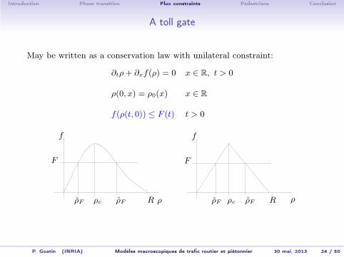
A toll gate
May be written as a conservation law with unilateral constraint:
∂tρ+ ∂xf(ρ) = 0 x ∈ R, t > 0
ρ(0, x) = ρ0(x) x ∈ R
f(ρ(t, 0)) ≤ F (t) t > 0
ρF ρFρc R
F
f
ρ ρF ρFρc R
F
f
ρ
P. Goatin (INRIA) Modèles macroscopiques de trafic routier et piétonnier 30 mai, 2013 24 / 50

Introduction Phase transition Flux constraints Pedestrians Conclusion
The Constrained Riemann Solver RF
(CRP)
∂tρ+ ∂xf(ρ) = 0ρ(0, x) = ρ0(x)f (ρ(t, 0)) ≤ F
ρ0(x) =
ρl if x < 0ρr if x > 0
Definition (Colombo-Goatin, 2007)
If f(R(ρl, ρr))(0)
)≤ F , then RF (ρl, ρr) = R(ρl, ρr).
Otherwise, RF (ρl, ρr)(x) =
R(ρl, ρF )(x) if x < 0 ,R(ρF , ρ
r)(x) if x > 0 .
=⇒ non-classical shock at x = 0
P. Goatin (INRIA) Modèles macroscopiques de trafic routier et piétonnier 30 mai, 2013 25 / 50
ρq ρqρc R
F
f
ρ ρq ρFρc R
F
f
ρ
ρl
ρr

Introduction Phase transition Flux constraints Pedestrians Conclusion
Entropy conditions
Definition (Colombo-Goatin, 2007)
ρ ∈ L∞ is weak entropy solution if
∀φ ∈ C1c , φ ≥ 0, and ∀k ∈ [0, R]
∫ +∞
0
∫
R
(|ρ− κ|∂t + Φ(ρ, κ)∂x) φ dx dt+
∫
R
|ρ0 − κ| φ dx
+ 2
∫ +∞
0
(
1−F (t)
f(ρc)
)
f(κ) φ(t, 0) dt ≥ 0
f(ρ(t, 0−)) = f(ρ(t, 0+)) ≤ F (t) a.e. t > 0
where Φ(a, b) = sgn(a− b)(f(a)− f(b))
(Cfr. conservation laws with discontinuous flux function:Karlsen-Risebro-Towers ’03, Karlsen-Towers ’04, Coclite-Risebro ’05...)
P. Goatin (INRIA) Modèles macroscopiques de trafic routier et piétonnier 30 mai, 2013 26 / 50

Introduction Phase transition Flux constraints Pedestrians Conclusion
Well-posedness in BV
constraint −→ TV(ρ) explosion
ρFρF
ρc ρc
t
x0
We consider the function
Ψ(ρ) = sgn(ρ− ρc)(f(ρc)− f(ρ))
(cfr. Temple ’82, Coclite-Risebro ’05 ...)
P. Goatin (INRIA) Modèles macroscopiques de trafic routier et piétonnier 30 mai, 2013 27 / 50

Introduction Phase transition Flux constraints Pedestrians Conclusion
Well-posedness in BV
Theorem (Colombo-Goatin, 2007)
F ∈ BV. There exists a semigroup SF : R+ ×D 7→ D s.t.
D ⊇ ρ ∈ L1 : Ψ(ρ) ∈ BV;
∥∥SF
t ρ1 − SFt ρ2
∥∥L1
≤ ‖ρ1 − ρ2‖L1 ∀ρ1, ρ2 ∈ D.
Proof
1 Wave-front tracking.
2 Glimm functional ad hoc
Υ(ρn, Fn) =∑
α
|Ψ(ρnα+1)−Ψ(ρnα)|+ 5∑
tβ≥0
∣∣Fn
β+1 − Fnβ
∣∣+ γ(ρn)
3 Doubling of variables method with constraint.
P. Goatin (INRIA) Modèles macroscopiques de trafic routier et piétonnier 30 mai, 2013 28 / 50

Introduction Phase transition Flux constraints Pedestrians Conclusion
Well-posedness in L∞
If F 1, F 2 ∈ L∞, ρ1, ρ2 ∈ L
∞ and ρ1 − ρ2 ∈ L1:
∫
R
|ρ1 − ρ2|(T, x) dx ≤ 2
∫ T
0
|F 1 − F 2|(t) dt +
∫
R
|ρ10 − ρ20|(x) dx
Theorem (Andreianov-Goatin-Seguin, 2010)
∀ρ0 ∈ L∞ and ∀F ∈ L
∞ ∃! weak entropy solution.
Proof
Truncation + regularization + finite propagation speed.
P. Goatin (INRIA) Modèles macroscopiques de trafic routier et piétonnier 30 mai, 2013 29 / 50
Introduction Phase transition Flux constraints Pedestrians Conclusion
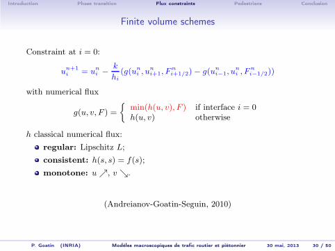
Finite volume schemes
Constraint at i = 0:
un+1i = un
i −k
hi(g(un
i , uni+1, F
ni+1/2)− g(un
i−1, uni , F
ni−1/2))
with numerical flux
g(u, v, F ) =
min(h(u, v), F ) if interface i = 0h(u, v) otherwise
h classical numerical flux:
regular: Lipschitz L;
consistent: h(s, s) = f(s);
monotone: uր, v ց.
(Andreianov-Goatin-Seguin, 2010)
P. Goatin (INRIA) Modèles macroscopiques de trafic routier et piétonnier 30 mai, 2013 30 / 50

Introduction Phase transition Flux constraints Pedestrians Conclusion
Example: toll gate
We consider∂tρ+ ∂x (ρ(1− ρ)) = 0
ρ(0, x) = 0.3χ[0.2,1](x)
f(ρ(t, 1)) ≤ 0.1
P. Goatin (INRIA) Modèles macroscopiques de trafic routier et piétonnier 30 mai, 2013 31 / 50

Introduction Phase transition Flux constraints Pedestrians Conclusion
Extensions
Second order models (Aw-Rascle)(Garavello-Goatin, 2011)
Rigorous study of general fluxes and non-classical problems(Chalons-Goatin-Seguin, 2013)
Improved numerical techniques for non-classical problems(Chalons-Goatin-Seguin, 2013)
Moving bottlenecks(DelleMonache-Goatin, 2012)
P. Goatin (INRIA) Modèles macroscopiques de trafic routier et piétonnier 30 mai, 2013 32 / 50

Introduction Phase transition Flux constraints Pedestrians Conclusion
Outline of the talk
1 Traffic flow models
2 Phase transition models
3 Flux constraints
4 Crowd dynamics
5 Conclusion
P. Goatin (INRIA) Modèles macroscopiques de trafic routier et piétonnier 30 mai, 2013 33 / 50

Introduction Phase transition Flux constraints Pedestrians Conclusion
Crowd dynamics
2D system modeling a crowd in a confined space:
∂tρ(t,x) + divxf(t,x) = 0 t > 0, x ∈ Ω ⊂ R2
+ boundary conditions
+ closure equation for the flux f
to reproduce known pedestrian behavior:
seeking the fastest route
avoiding high densities and borders
lines formation in opposite fluxes
collective auto-organization at intersections
behavior changes in panic situations and becomes irrational
etc ...
P. Goatin (INRIA) Modèles macroscopiques de trafic routier et piétonnier 30 mai, 2013 34 / 50

Introduction Phase transition Flux constraints Pedestrians Conclusion
Hughes’ model (2002)
Mass conservation
∂tρ+ divx
(
ρ~V (ρ))
= 0 in R+ × Ω
where
~V (ρ) = v(ρ) ~N and v(ρ) = vmax
(
1−ρ
ρmax
)
Direction of the motion: ~N = −∇φ
|∇φ|is given by
|∇φ| =1
v(ρ)in Ω
φ(t,x) = 0 for x ∈ ∂Ωexit
pedestrians tend to minimize their estimated travel time to the exit
pedestrians temper their estimated travel time avoiding high densities
CRITICS: instantaneous global information on entire domain
P. Goatin (INRIA) Modèles macroscopiques de trafic routier et piétonnier 30 mai, 2013 35 / 50

Introduction Phase transition Flux constraints Pedestrians Conclusion
Dynamic model with memory effectMass conservation
∂tρ+ divx
(
ρ~V (ρ))
= 0 in R+ × Ω
where
~V (ρ) = v(ρ) ~N and v(ρ) = vmax
(
1−ρ
ρmax
)
Direction of the motion: ~N = −∇x(φ+ ωD)
|∇x(φ+ ωD)|where
|∇xφ| =1
vmaxin Ω, φ(x) = 0 for x ∈ ∂Ωexit,
D = D(ρ) =1
v(ρ)+ βρ2 discomfort
pedestrians seek to minimize their estimated travel time based on theirknowledge of the walking domain
pedestrians temper their behavior locally to avoid high densities
(Xia-Wong-Shu, 2009)
P. Goatin (INRIA) Modèles macroscopiques de trafic routier et piétonnier 30 mai, 2013 36 / 50

Introduction Phase transition Flux constraints Pedestrians Conclusion
Second order model
Euler equations with relaxation
∂tρ+∇ · (ρ~V ) = 0
∂t(ρ~V ) +∇ · (ρ~V ⊗ ~V ) =1
τ(ρve(ρ) ~N − ρ~V )
︸ ︷︷ ︸
relaxationterm
+ ∇P (ρ)︸ ︷︷ ︸
anticipationfactor
where
ve(ρ) = vmax exp
(
−α
(ρ
ρmax
)2)
, P (ρ) = p0ργ
and boundary conditions: ∇xρ · ~n = 0 and ~V · ~n = 0
(Jiang-Zhang-Wong-Liu, 2010)
P. Goatin (INRIA) Modèles macroscopiques de trafic routier et piétonnier 30 mai, 2013 37 / 50
Introduction Phase transition Flux constraints Pedestrians Conclusion
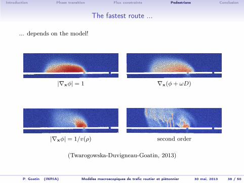
The fastest route ...
... depends on the model!
|∇xφ| = 1 ∇x(φ+ ωD)
|∇xφ| = 1/v(ρ) second order
(Twarogowska-Duvigneau-Goatin, 2013)
P. Goatin (INRIA) Modèles macroscopiques de trafic routier et piétonnier 30 mai, 2013 38 / 50

Introduction Phase transition Flux constraints Pedestrians Conclusion
The fastest route ...
... depends on the model!
|∇xφ| = 1 ∇x(φ+ ωD)
|∇xφ| = 1/v(ρ) second order
(Twarogowska-Duvigneau-Goatin, 2013)
P. Goatin (INRIA) Modèles macroscopiques de trafic routier et piétonnier 30 mai, 2013 38 / 50

Introduction Phase transition Flux constraints Pedestrians Conclusion
The fastest route ...
... depends on the model!
|∇xφ| = 1 ∇x(φ+ ωD)
|∇xφ| = 1/v(ρ) second order
(Twarogowska-Duvigneau-Goatin, 2013)
P. Goatin (INRIA) Modèles macroscopiques de trafic routier et piétonnier 30 mai, 2013 38 / 50

Introduction Phase transition Flux constraints Pedestrians Conclusion
The fastest route ...
... depends on the model!
|∇xφ| = 1 ∇x(φ+ ωD)
|∇xφ| = 1/v(ρ) second order
(Twarogowska-Duvigneau-Goatin, 2013)
P. Goatin (INRIA) Modèles macroscopiques de trafic routier et piétonnier 30 mai, 2013 38 / 50
Introduction Phase transition Flux constraints Pedestrians Conclusion
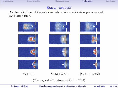
Braess’ paradox?
A column in front of the exit can reduce inter-pedestrians pressure andevacuation time?
|∇xφ| = 1 ∇x(φ+ ωD) |∇xφ| = 1/v(ρ)
(Twarogowska-Duvigneau-Goatin, 2013)
P. Goatin (INRIA) Modèles macroscopiques de trafic routier et piétonnier 30 mai, 2013 39 / 50

Introduction Phase transition Flux constraints Pedestrians Conclusion
Braess’ paradox?
Evacuation time:
(Twarogowska-Duvigneau-Goatin, 2013)
P. Goatin (INRIA) Modèles macroscopiques de trafic routier et piétonnier 30 mai, 2013 40 / 50

Introduction Phase transition Flux constraints Pedestrians Conclusion
Braess’ paradox?
The second order model displays a better behavior:
(Twarogowska-Duvigneau-Goatin, 2013)
P. Goatin (INRIA) Modèles macroscopiques de trafic routier et piétonnier 30 mai, 2013 41 / 50

Introduction Phase transition Flux constraints Pedestrians Conclusion
Braess’ paradox?
Evacuation time:
(Twarogowska-Duvigneau-Goatin, 2013)
P. Goatin (INRIA) Modèles macroscopiques de trafic routier et piétonnier 30 mai, 2013 42 / 50

Introduction Phase transition Flux constraints Pedestrians Conclusion
The 1D case: statement of the problem
Rigorous (preliminary) results:We consider the initial-boundary value problem
ρt −
(
ρ(1− ρ)φx
|φx|
)
x
= 0
|φx| = c(ρ)
x ∈ Ω = ]− 1, 1[, t > 0
with initial density ρ(0, ·) = ρ0 ∈ BV(]0, 1[)and absorbing boundary conditions
ρ(t,−1) = ρ(t, 1) = 0 (weak sense)φ(t,−1) = φ(t, 1) = 0
P. Goatin (INRIA) Modèles macroscopiques de trafic routier et piétonnier 30 mai, 2013 43 / 50

Introduction Phase transition Flux constraints Pedestrians Conclusion
The 1D case: statement of the problem
Rigorous (preliminary) results:We consider the initial-boundary value problem
ρt −
(
ρ(1− ρ)φx
|φx|
)
x
= 0
|φx| = c(ρ)
x ∈ Ω = ]− 1, 1[, t > 0
with initial density ρ(0, ·) = ρ0 ∈ BV(]0, 1[)and absorbing boundary conditions
ρ(t,−1) = ρ(t, 1) = 0 (weak sense)φ(t,−1) = φ(t, 1) = 0
General cost function c : [0, 1[ → [1,+∞[ smooth s.t. c(0) = 1 and c′(ρ) ≥ 0(e.g. c(ρ) = 1/v(ρ))
P. Goatin (INRIA) Modèles macroscopiques de trafic routier et piétonnier 30 mai, 2013 43 / 50
Introduction Phase transition Flux constraints Pedestrians Conclusion
The 1D case: statement of the problem
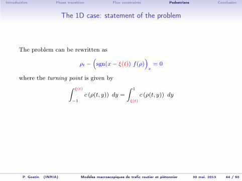
The problem can be rewritten as
ρt −(
sgn(x− ξ(t)) f(ρ))
x= 0
where the turning point is given by
∫ ξ(t)
−1
c (ρ(t, y)) dy =
∫ 1
ξ(t)
c (ρ(t, y)) dy
P. Goatin (INRIA) Modèles macroscopiques de trafic routier et piétonnier 30 mai, 2013 44 / 50

Introduction Phase transition Flux constraints Pedestrians Conclusion
The 1D case: statement of the problem
The problem can be rewritten as
ρt −(
sgn(x− ξ(t)) f(ρ))
x= 0
where the turning point is given by
∫ ξ(t)
−1
c (ρ(t, y)) dy =
∫ 1
ξ(t)
c (ρ(t, y)) dy
−→ the discontinuity point ξ = ξ(t) is not fixed a priori,but depends non-locally on ρ
P. Goatin (INRIA) Modèles macroscopiques de trafic routier et piétonnier 30 mai, 2013 44 / 50

Introduction Phase transition Flux constraints Pedestrians Conclusion
The 1D case: preliminary results
existence and uniqueness of Kruzkov’s solutions for an ellipticregularization of the eikonal equation and c = 1/v(DiFrancesco-Markowich-Pietschmann-Wolfram, 2011)
P. Goatin (INRIA) Modèles macroscopiques de trafic routier et piétonnier 30 mai, 2013 45 / 50

Introduction Phase transition Flux constraints Pedestrians Conclusion
The 1D case: preliminary results
existence and uniqueness of Kruzkov’s solutions for an ellipticregularization of the eikonal equation and c = 1/v(DiFrancesco-Markowich-Pietschmann-Wolfram, 2011)
Riemann solver at the turning point for c = 1/v(Amadori-DiFrancesco, 2012)
entropy condition and maximum principle
(ElKhatib-Goatin-Rosini, 2012)
wave-front tracking algorithm and convergence of finite volumeschemes(Goatin-Mimault, 2013)
P. Goatin (INRIA) Modèles macroscopiques de trafic routier et piétonnier 30 mai, 2013 45 / 50

Introduction Phase transition Flux constraints Pedestrians Conclusion
The 1D case: entropy condition
Definition: entropy weak solution (ElKhatib-Goatin-Rosini, 2012)
ρ ∈ C0(R
+;L1(Ω))∩ BV (R+ × Ω; [0, 1]) s.t. for all k ∈ [0, 1] and
ψ ∈ C∞c (R×Ω;R+):
0 ≤
∫ +∞
0
∫ 1
−1
(|ρ− k|ψt + Φ(t, x, ρ, k)ψx) dx dt+
∫ 1
−1
|ρ0(x)− k|ψ(0, x) dx
+ sgn(k)
∫ +∞
0
(f (ρ(t, 1−))− f(k))ψ(t, 1) dt
+ sgn(k)
∫ +∞
0
(f (ρ(t,−1+))− f(k))ψ(t,−1) dt
+ 2
∫ +∞
0
f(k)ψ (t, ξ(t)) dt.
where Φ(t, x, ρ, k) = sgn(ρ− k) (F (t, x, ρ)− F (t, x, k))
P. Goatin (INRIA) Modèles macroscopiques de trafic routier et piétonnier 30 mai, 2013 46 / 50
Introduction Phase transition Flux constraints Pedestrians Conclusion
The 1D case: maximum principle
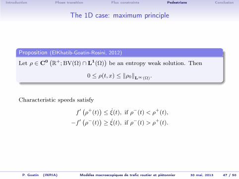
Proposition (ElKhatib-Goatin-Rosini, 2012)
Let ρ ∈ C0(R
+;BV(Ω) ∩ L1(Ω)
)be an entropy weak solution. Then
0 ≤ ρ(t, x) ≤ ‖ρ0‖L∞(Ω).
Characteristic speeds satisfy
f ′(ρ+(t)
)≤ ξ(t), if ρ−(t) < ρ+(t),
−f ′(ρ−(t)
)≥ ξ(t), if ρ−(t) > ρ+(t).
P. Goatin (INRIA) Modèles macroscopiques de trafic routier et piétonnier 30 mai, 2013 47 / 50

Introduction Phase transition Flux constraints Pedestrians Conclusion
Outline of the talk
1 Traffic flow models
2 Phase transition models
3 Flux constraints
4 Crowd dynamics
5 Conclusion
P. Goatin (INRIA) Modèles macroscopiques de trafic routier et piétonnier 30 mai, 2013 48 / 50
Introduction Phase transition Flux constraints Pedestrians Conclusion
Perspectives
Sound analytical basis for practical implementation:
ROAD TRAFFIC :
finite acceleration for pollution models
ramp metering and rerouting models
optimal control techniques for traffic management
(ORESTE Associated Team with UC Berkeley)
PEDESTRIANS :
well-posedness
validation against empirical data
shape optimization for architecture and urban planning
P. Goatin (INRIA) Modèles macroscopiques de trafic routier et piétonnier 30 mai, 2013 49 / 50

Introduction Phase transition Flux constraints Pedestrians Conclusion
Thank you for your attention!
P. Goatin (INRIA) Modèles macroscopiques de trafic routier et piétonnier 30 mai, 2013 50 / 50