KODERP! DEVELOPMENTS I N CHI-SQUARE GOODNESS-OF-FIT TESTING

Dora Hutchinson

B.Sc. Simon Fraser U n i v e r s i t y 1977

A THESIS SUBMITTED I N PARTIAL FULFILLMENT OF

THE REQUIREMENTS FOR THE DEGREE OF

YASTER OF SCIENCE

i n t h e Department

o f

Mathematics

@ Dora Hutchinson 1983

SIMON FRASER UNIVERSITY

May 1983

A l l r i g h t s reserved. Th i s t h e s i s may n o t be reproduced i n whole o r i n p a r t , by photocopy o r o t h e r means, w i t h o u t permiss ion o f t h e author .

APPROVAL

Name: Dora Hutchinson

Degree: Master of Science

Ti t le of thesis : Modern Developments in Chi-square Goodness-of-Fit Testing

Exami ni ng Committee :

Chairman: B.S. Thomson

R . Lockhart Senior Supervi sor

M .A. ~tebhens

P.M. Eaves

R . Routledge External Examiner

Department of Matheli iat ics Simon Fraser University

Date Approved: April 13, 1983

PARTIAL COPYRIGHT LICENSE

I hereby g r a n t t o Simon Fraser U n i v e r s i t y t h e r i g h t t o l end

my t h e s i s o r d i s s e r t a t i o n ( t h e t i t l e o f which i s shown below) t o users

o f t h e Simon Fraser U n i v e r s i t y L i b r a r y , and t o make p a r t i a l o r s i n g l e

cop ies o n l y f o r such users o r i n response t o a reques t f rom t h e l i b r a r y

i t s own

i o n f o r

g ran ted

copy ing

a1 lowed

o f any o t h e r u n i v e r s i t y , o r o t h e r educa t iona l i n s t i t u t i o n ,

b e h a l f o r f o r one o f i t s users . I f u r t h e r agree t h a t perm

m u l t i p l e copy ing o f t h i s t h e s i s f o r s c h o l a r l y purposes may

on

i ss

be

by me o r t h e Dean o f Graduate S tud ies . I t i s understood t h a t

o r p u b l i c a t i o n o f t h i s t h e s i s f o r f i n a n c i a l ga i n s h a l l n o t be

w i t h o u t my w r i t t e n permiss ion.

T i tl e o f Thesi s /Di s s e r t a t i on :

Modern Developments i n Chi-square Goodness-of-Fit Tes t i ng

Author :

Dora Hutch inson

(name)

A p r i l 18, 1983

(da te )

ABSTRACT

MODERN DEVELOPMENTS I N CHI-SQUARE GOODNESS-OF-FIT TESTING

An exam

s t a t i s t i c i s

i n a t i o n o f t h e h i s t o r i c a l deve lopment o f t h e Pearson c h i - s q u a r e

p r e s e n t e d f o l l o w e d b y a r e v i e w o f t h e r e c e n t

n i q u e s i n t h e f i e l d o f c h i - s q u a r e g o o d n e s s - o f - f i t t e s t i n g

s t u d y o f t h e new s t a t i s t i c s ( t h e Rao-Robson s t a t i s t i c and

l y deve loped t e c h -

. I n p a r t i c u l a r , a

t h e Dzhapar idze-

Ni k u l i n s t a t i s t i c ) c l a i m i n g t o o f f e r improvement o v e r Pearson ' s x 2 i s p r o v i d e d ;

Monte C a r l o p o i n t s f o r t h e s e s t a t i s t i c s f o r f i n i t e n a r e de te rm ined , power

s t u d i e s a r e per formed and compar isons drawn between c o m p e t i t o r s , and t e s t

p rocedures a r e a p p l i e d t o r e a l d a t a t o i l l u s t r a t e t h e i r usage. F i n a l l y ,

c o n c l u s i o n s a r e drawn as t o t h e success o f t h e modern c h i - s q u a r e methods and

a summary o f t h e i r c u r r e n t a p p l i c a b i l i t y g i v e n .

ACKNOWLEDGEMENTS

I wish t o extend my s ince re a p p r e c i a t i o n and g r a t i t u d e t o my Senior

Superv isor , Dr. R. Lockhart , f o r making t h e comple t ion o f t h i s paper a

much e a s i e r task . Thanks a l s o go t o D r . M.A. Stephens f o r h i s many h e l p f u l

suggest ions.

My acknowledgements would n o t be complete w i t h o u t recogn iz ing my s i s t e r

Jan f o r her i n v a l u a b l e c o n t r i b u t i o n s t o t h e t y p i n g and o r g a n i z a t i o n o f t h i s

work.

TABLE OF CONTENTS

Approval . . . . . . . . . . . . . . . . . . . . . . . . . . . . ii

A b s t r a c t . . . . . . . . . . . . . . . . . . . . . . . . . . . . i i i

Acknowledgements . . . . . . . . . . . . . . . . . . . . . . . . i v

L i s t o f Tables . . . . . . . . . . . . . . . . . . . . . . . . . v i

I. I n t r o d u c t i o n . . . . . . . . . . . . . . . . . . . . . . . . . . 1

11. The H i s t o r i c a l Development o f t h e Chi-square Goodness-of-Fi t S t a t i s t i c . . . . . . . . . . . . . . . . . . . 3

111. Modern Methods . . . . . . . . . . . . . . . . . . . . . . . . . 17

. . . . . . . . . . . . . . . . . . . . . I V . P r a c t i c a l App l i ca t i ons 57

V. Monte Car lo Po in t s f o r F i n i t e Sample S i ze . . . . . . . . . . . 61

V I . Power Comparisons . . . . . . . . . . . . . . . . . . . . . . . 81 .

. . . . . . . . . . . . . . . . . . . . . . . . . V I I . Conclusions . 8 9

Append ix . . . . . . . . . . . . . . . . . . . . . . . . . . . . 91

Bib1 iography . . . . . . . . . . . . . . . . . . . . . . . . . .I12

LIST OF TABLES

. . . . . . . . . . . . . The Normal D i s t r i b u t i o n . n = 20 k = 4

= . . . . . . . . . . . . . The Normal D i s t r i b u t i o n . n = 50 k 10

. . . . . . . . . . . . . The Normal D j s t r i b u t i o n . n = 100 k = 10

. . . . . . . . . . . The Exponential D i s t r i b u t i o n . n = 20 k = 4

. . . . . . . . . . The Exponential D i s t r i b u t i o n . n = 50 k = 10

. . . . . . . . . . The Exponential D i s t r i b u t i o n . n = 100 k = 10

. . . . . . . The Double Exponential D i s t r i b u t i o n . n = 20 k = 4

. . . . . . . The Double Exponent ia l D i s t r i b u t i o n . n = 53 k = 10

. . . . . . . The Double Exponent ia l D i s t r i b u t i o n . n = 100 k = 10

. . . . . . . The C i r c u l a r B i v a r i a t e D i s t r i b u t i o n . n = 20 k = 4

. . . . . . . The C i r c u l a r B i v a r i a t e D i s t r i b u t i o n . n = 50 k = 8

. . . . . . . The C i r c u l a r B i v a r i a t e D i s t r i b u t i o n . n = 100 k = 10

= . . . . . . . . . . . . The L o g i s t i c D i s t r i b u t i o n . n = 20 k 4

. . . . . . . . . . . . The L o g i s t i c D i s t r i b u t i o n . n = 50 k = 8

. . . . . . . . . . . . The L o g i s t i c D i s t r i b u t i o n . n = 100 k = 10

. . . . . . . . . . The Extreme Value D i s t r i b u t i o n . n = 20 k = 4

The Extreme Value D i s t r i b u t i o n . n = 50 k = 8 . . . . . . . . . . . . . . . . . . . The Extreme Value D i s t r i b u t i o n . n = 100 k = 10

Power Comparisons. Normal D i s t r i b u t i o n . . . . . . . . . . . . . . Power Comparisons. Exponent ia l D i s t r i b u t i o n . . . . . . . . . . .

. . . . . . . . Power Comparisons. Double Exponent ia l D i s t r i b u t i o n

. . . . . . . . Power Comparisons. C i r c u l a r B i v a r i a t e D i s t r i b u t i o n

Power Comparisons. L o g i s t i c D i s t r i b u t i o n . . . . . . . . . . . . . Power Comparisons. Extreme Val ue D i s t r i b u t i o n . . . . . . . . . .

I. INTRODUCTION

Since i t was f i r s t proposed i n 1900, Ka r l Pearson 's ch i -square s t a t i s t i c

has become one o f t h e most popu la r techn iques i n g o o d n e s s - o f - f i t t e s t i n g today.

However, though t h e r e a r e s i t u a t i o n s where t h e ch i - squa re s t a t i s t i c i s i d e a l

and i r r e p l a c e a b l e , i t s f l e x i b i l i t y and ease o f computa t ion a r e o f t e n n o t

s u f f i c i e n t t o w a r r a n t i t s use, and t h e t r e n d i s towards t h e use o f more power-

f u l g o o d n e s s - o f - f i t s t a t i s t i c s . Pearson 's s t a t i s t i c , denoted by x2, has been

unable t o compete w i t h t hese s t a t i s t i c s i n many s i t u a t i o n s due t o t h e f a c t

t h a t i t does n o t use t h e t o t a l i n f o r m a t i o n g i v e n by t h e i n d i v i d u a l da ta p o i n t s ;

i t cons ide rs o n l y t h e number o f obse rva t i ons f a l l i n g w i t h i n s p e c i f i e d c e l l s and

consequent ly l a c k s power.

Recen t l y t h e r e have been a t t emp ts made t o overcome some o f t h e d i f f i c u l -

t i e s h i s t o r i c a l l y a s s o c i a t e d w i t h Pearson 's s t a t i s t i c which have inc reased

ch i - squa re ' s s t a t u r e i n g o o d n e s s - o f - f i t t e s t i n g . Some ques t ions t h a t have

been o f i n t e r e s t i n t h e p a s t such as "How can degrees o f freedom l o s t due t o -

parameter e s t i m a t i o n be recovered?" and "How shou ld t h e unknown parameters be

es t imated?" a r e b e i n g r e - e v a l u a t e d i n t h e 1 i gh t o f new s t a t i s t i c a l approaches.

Th i s paper s e t s o u t t o examine t hese new techn iques w i t h t h e i n t e n t i o n o f

de te rm in i ng how t h e y have improved on Pearson 's ch i - squa re s t a t i s t i c i n

goodness -o f - f i t t e s t i n g and t o a s c e r t a i n how good these improvements a r e i n

terms o f i n c reased power and /o r app l i c a b i l i t y .

Pa r t I 1 dea ls w i t h t h e h i s t o r i c a l development o f t h e ch i - squa re s t a t i s t i c

s i n c e 1900, examin ing t h e t h e o r y beh ind i t , t h e problems encountered, and t h e

e x i s t i n g s o l u t i o n s t o t h e s e problems. A r e v i e w o f t h e o l d method s u f f i c i e n t

t o prepare f o r an exam ina t i on o f t h e new methods i s p rov ided . Desp i t e i t s

l o n g ex is tence , i t i s s t i l l u s e f u l .

Part I11 takes a look a t the l a t e s t developments and provides an i n -

depth study of a selection of the more promising techniques.

Part IV presents some practical applications of the new s t a t i s t i c s , and

Part V provides tabled Monte Carlo points for the new s t a t i s t i c s determined

for f i n i t e n . Part VI examines the comparative power of the new s t a t i s t i c s

against selected al ternat ives .

Finally, in Part VII, conclusions are drawn as t o the success of the

modern chi-square techniques and a summary of t h e i r current appl icabi l i ty

given.

I I . THE HISTORICAL DEVELOPMENT O F THE C H I - S Q U A R E

GOODNESS-OF-FIT STATISTIC

A problem frequently a r i s ing in s t a t i s t i c s i s the goodness-of-fit problem

where we wish to t e s t whether or not a random variable X i s distributed accord-

ing to a par t icular dis t r ibut ion function F o ( x ) F o ( x ) may be a completely

specified function (e.g. F (x) i s the Normal dis t r ibut ion function with mean 0

% and variance 0:) or i t may be only par t ia l ly specified (e.g. F o ( x ) i s in

the normal family of dis t r ibut ions .)

The famous s t a t i s t i c , x2 , tha t Karl Pearson proposed in 1900 i s frequently

used t o tackle t h i s problem. I t i s a favourite due to i t s ease of application

and the abundant ava i l ab i l i t y of tabled values for the Chi-square dis t r ibut ion.

2 Pearson's X was developed on the basis of measuring whether or n o t the

observed frequencies of observations on the variable X f a l l i ng into "cel ls"

were consistent with the "expected" frequencies; tha t i s , the number of

observations we would expect to observe given tha t F ( x ) i s indeed the t rue 0

2 distr ibut ion function. The theory underlying Pearson's X s t a t i s t i c i s

dependent on whether or not the hypothesized dis t r ibut ion function Fo(x) i s

completely specified ( the Simple Hypothesis Case) or only par t ia l ly specified

(the Composite Hypothesis Case) and requires parameter estimation.

1 A . The Simple Hypothesis Case I I i

i Suppose we are in a goodness-of-fit s i tua t ion where we wish t o t e s t the !

1 simple hypothesis H o : F(x) = F ( x ) where F (x) i s completely specified. We 0 0

* 1 assume a random sample of n independent observations on the random variable X

has been gathered, and tha t we have a r b i t r a r i l y divided the range of X into k

: mutually exclusive c e l l s ( the actual selection of these ce l l s will be

considered l a t e r ) . Let - X ' denote the row vector of observations, so that

4

X I = (x , . x, ...... , x ) . We can now ca l cu l a t e N' = (N, . N2 ...... ,N ) where N i - n k

denotes the number of observations f a l l i n g i n to the i t h c e l l , f o r i = l , . .. , k .

These Nils cons t i t u t e a sample of k observations from the blul tinomial d i s t r i -

bution. If we assume tha t the null hypothesis i s t r ue , we can immediately

f ind the probabi l i ty pi t h a t an observation will f a l l i n to the i th c e l l , and

subsequently t he j o i n t probabi l i ty t h a t n, observations f a l l i n to the f i r s t

...... c e l l , n, observations f a l l in to the second c e l l , and n k observations

fa1 1 i n to the k t h c e l l . The mul t ivar ia te form of the Central Limit Theorem s t a t e s t h a t N' wil l

tend, a s n goes t o i n f i n i t y , t o have a Normal d i s t r i bu t i on with mean - p , where

p = ( n p , . np,, ..... ,npk) , and dispersion matrix V , where -

This matrix V i s of dimension k , b u t s ince we have the r e s t r i c t i o n t ha t the

sum of the N i Is i s equal t o n , V i s of rank k - 1 and hence i s not inver t ib le .

Since the theory requires t h a t V be i nve r t i b l e , we overcome t h i s problem by

dele t ing a row and column, say the l a s t row and the 1 a s t column, and will c a l l

t h i s new matrix V*.

The inverse of V* i s then:

The quadratic form Q of the exponent of the Multivariate Normal dis t r ibut ion,

general form, i s then given by:

Q = (N - - ~-)'v*-l(N- -

This can be reduced algebraically as follows:

2 This l a s t expression i s , of course, Pearson's chi-square s t a t i s t i c X . 2

Hence, X i s asymptotically chi-square dis t r ibuted with k - 1 degrees of freedom.

This resu l t follows from the theory of the Multivariate Normal dis t r ibut ion

which s t a t e s tha t the quadratic form in the exponent of t h i s dis t r ibut ion i s

chi-square dis t r ibuted with degrees of freedom equal to the rank of V*, in t h i s

case k - 1 .

An a l te rna t ive proof of the same conclusion tha t avoids any mathematical.

complexities (and i s a popular item in reviews of chi-square theory) i s

Fisher 's famous proof of 1922. For a l l i t s s implici ty , i t proves t o be

extremely enlightening for reasons tha t will l a t e r become obvious when the

Composite Hypothesis Case i s considered.

Suppose we have t h a t x , , x2 , . . . . . , xk are k independent Poisson distributed

variates , the i t h vari a te having parameter npi associated with i t . Then, the

probability t h a t xl=N1, x2=N2 ,. . . . . , X = N i s just k k

The sum of the k independent Poisson var ia tes , denoted here by S , i s k

Poisson distributed with parameter 1 n p i = n . Hence, the probability of S i =l

being equal to n i s :

We can now find the probability tha t x l = n l , x2= n 2 , . . . . . , X = n conditional on k k

This we recognize as the Mul t inomia l d i s t r i b u t i o n . I f we def ine

- - 1,2 ,....., k - Y i - Ni - np f o r i i

b p i 1%

then as n goes t o i n f i n i t y , t he d i s t r

d i s t r i b u t i o n w i t h mean 0 and var iance

i b u t i o n o f yi approaches the Normal

2 1. Since X can be expressed as the sum

o f these k independent s tandard normal v a r i a t e s sub jec t t o the s i n g l e l inear

c o n s t r a i n t S=n, we can now e s t a b l i s h , by q u o t i n g well-known theorems, t h a t i n

2 the l i m i t X f o l l o w s the Chi-square d i s t r i b u t i o n w i t h k -1 degrees o f freedom.

This concl udes F i sher ' s p roo f .

The r e v e a l i n g aspect w i l l be apprec ia ted more f u l l y i n t h e s e c t i o n on

parameter es t imat ion , f o l l o w i n g , where each parameter t o be est imated imposes

an a d d i t i o n a l l i n e a r c o n s t r a i n t .

B. The Composite Hypothesis Case

Suppose now t h a t we a r e i n t h e s i t u a t i o n where we w ish t o t e s t t he

composite hypothesis Ho: F (x ) = Fo(x) where Fo(x) i s a cont inuous d i s t r i b u -

t i o n n o t t o t a l l y s p e c i f i e d b u t having s o f i t s parameters unknown. The

imnediate consequence here versus t h e Simple Hypothesis Case i s t h a t the

requ i red p r o b a b i l i t i e s pi, i = l , ....., k, a r e no l o n g e r ca l cu lab le , a t l e a s t

p r i o r t o observ ing t h e data. I f we denote t h e s unknown parameters o f t he

d i s t r i b u t i o n func t i on Fo(x) as 0, ,0,,. . . . . ,es, then the pi I s a re themselves

funct ions of a' = (0, ,e,,. . . . . , e S ) To emphasize t h i s r e l a t i o n s h i p , the

9

2 unknown p r o b a b i l i t i e s w i l l be denoted by p.(e). To c a l c u l a t e X i n t h i s 1 -

s i t u a t i o n , now o f t h e form

we w i l l r e q u i r e est imates of the unknown parameters, These est imates w i l l

here be denoted c o l l e c t i v e l y by - 6 = ( 6 1 , G 2 ,....., gS) .

This presents a new d i s t r i b u t i o n problem, f o r i t i s n o t obvious t h a t t h e

asymptot ic d i s t r i b u t i o n o f t h i s s t a t i s t i c w i l l be o f t h e same form as i n t he

Simple Hypothesis Case. Pearson h i m s e l f d i d n o t be l i eve t h a t t he es t ima t ion

of unknown parameters us ing t h e sample data would s i g n i f i c a n t l y a1 t e r t he

2 d i s t r i b u t i o n o f h i s s t a t i s t i c . He be l i eved t h a t regard ing X as chi -square

d i s t r i b u t e d w i t h k -1 degrees o f freedom when unknown parameters were est imated

would cause o n l y n e g l i g i b l e e r r o r i n t h e approximat ion and would not ,

there fore , a f f e c t p r a c t i c a l dec is ions . H is conc lus ion was perhaps j u s t i f i e d

f o r some app l i ca t i ons , b u t h i s s t a t i s t i c performed so p o o r l y i n some o f t h e - 2 most common t e s t s employing X t h a t a "degrees-of-freedom b a t t l e " ensued. It

was n o t u n t i l 1924 w i t h t h e appearance o f F i s h e r ' s famous paper on the sub jec t

t h a t t he b a t t l e was resolved.

The Est imat ion o f Parameters

I f we now recons ider F i s h e r ' s p r o o f i n the Simple Hypothesis Case, we can

regard the es t ima t ion o f unknown parameters as s imply the i m p o s i t i o n of a

f u r t h e r s l i n e a r c o n s t r a i n t s . Th i s c l e a r l y has the e f f e c t o f reduc ing the

degrees o f freedom from k-1 t o k-s-1. However, t h i s conc lus ion tu rns o u t t o

be f u r t h e r dependent on the method o f es t ima t ion used.

The common estimators will be considered here, namely the Maximum Yulti-

nomial Likelihood estimators and the ?laximum Density Li kel ihood estimators.

We will discover tha t i f the Maximum Multinomial Likelihood ( M M L ) estimates

are employed (calculated by maximizing the jo in t density of the N i I s ) then a

further s l inear constraints a re imposed as suspected, and the degrees of

freedom are reduced to k-s-1 accordingly. These estimates, however, are

rarely ever used because of the d i f f i c u l t i e s associated with the i r computation.

By far the most popular method of estimation i s that based on maximizing

the joint density of the x i ' s . This method yields the Raximum Density Likeli-

hood (MDL) estimators, and in t h i s s i tua t ion , the reduction in the degrees of

freedom i s considerablv more cnmplicated. We will discover through the

following analysis tha t the degrees of freedom are bounded by k - 1 and k-s-1,

b u t beyond tha t we can draw no fur ther conclusions. If k i s large, then t h i s

difference i s negligible, b u t for small k , e r rors due to the difference between

the c r i t i ca l points for these two dis t r ibut ions will be s igni f icant .

A further investigation into the conditions which lead to a reduction i n -

the degrees of freedom i s provided by Watson in his paper of 1959 where he

gives a general approach t o the problem. A good review of the theory as

applied to Pearson's X' s t a t i s t i c i s presented by Kendall and Stuart (1963),

pages 425-430.

Kendall and Stuart show tha t i f we have estimators with variances and

2 covariances of order n m 2 , then X i s asymptotically chi-square distributed with

k - 1 degrees of freedom. However, t h i s i s n o t the usual case. Generally, we

have that 6 - 0 = ~(n- ' ) , and i t i s in t h i s s i tua t ion tha t they present t h e i r

theory.

I n the Simple Hypothesis Case, with y defined as:

- N i - npi (F) where yi -

they show that the dispersion matrix V ( 1 ) has a trace equal to k-1 so t h a t X 2

i s chi-square distributed with k-1 degrees of freedom in the limit.

I n the Composite Hypothesis Case, the theory i s more complicated, and the

resul t s are gi ven below according t o the particular estimates being considered.

a . The Maximum Mu1 tinomial Likelihood Estimators

The Mu1 tinomial Li kel ihood, L , i s :

To maximize L with respect to the unknown parameters s, the log

computed and then minimized by setting the f i r s t partial derivat

This gives:

likelihood i s

i ves t o zero.

k a i o g ~ = c N~ api 1

-- = 0 for j = 1 , 2 ,...,., s a e j

i=l a e . p 3 i

The roots of these s equations will provide the MML estimators. Note t h a t each

equation i s a homogeneous 1 inear relationship with respect t o the Nils so that

together they impose s additional 1 i near constraints within Fisher's proof

2 Presented ear l ier . Hence, X i s asymptotically chi-square distributed with

k-s-1 degrees of freedom.

Kendall and S t u a r t show t h a t i f these es t imates a r e used, then the

d ispers ion m a t r i x o f y (de f ined on page l l ) , V ( l ) , has a t r a c e equal t o k-s-1

2 imp ly ing t h a t X i s ch i -square d i s t r i b u t e d i n t h e l i m i t w i t h k-s-1 degrees o f

freedom.

The Maximum Mul t inomia l L i k e l i h o o d es t imates determined f rom the grouped

data are d i f f i c u l t t o ob ta in . For t h i s reason, when t h e i n d i v i d u a l data

po in t s a r e a v a i l a b l e , they a r e n o t used i n p r a c t i c e . Rather, t he Maximum

Density L i k e l i h o o d est imates obta ined f rom t h e ungrouped data a r e u t i l i z e d .

The use o f these MDL est imates a l s o i m p l i e s more e f f i c i e n t use o f the informa-

t i o n prov ided by the data g iven t h a t t h e ungrouped observa t ions a r e ava i l ab le .

b. The Maximum Dens i t y L ike1 ihood Est imators

The Dens i t y L i ke l i hood , LD, i s LD = f ( x l ) * - - = f ( x n ) where xi,

i = l , ....., n a r e independent observa t ions on t h e random v a r i a b l e X w i t h

p r o b a b i l i t y d e n s i t y f u n c t i o n f. The Maximum Dens i t y L i k e l i hood es t imators

are obta ined by maximizing LD and a r e g i ven by t h e r o o t s o f t h e equat ions:

Kendall and S t u a r t show t h a t i f these est imates a r e used, then the

d ispers ion m a t r i x o f 1, V(y), has a t r a c e bounded by k-s-1 and k -1 so t h a t i n

2 the l i m i t , t h e d i s t r i b u t i o n o f X i s n o t chi-square, b u t i s bounded between a

Chi-square d i s t r i b u t i o n w i t h k-s-1 degrees of freedom and a Chi-square

d i s t r i b u t i o n w i t h k-1 degrees o f freedom. Hence, f o r l a r g e k , t h e e f fec t of

us ing the Chi-square d i s t r i b u t i o n w i t h k-s-1 degrees o f freedom i n goodness-

o f - f i t t e s t i n g w i l l n o t l e a d t o se r ious e r r o r . However, an examinat ion of a

1 t a b l e o f Chi-square d i s t r i b u t i o n values w i l l show t h a t t h i s i s n o t t h e case

for small k , and t h i s f a c t should be kept i n mind f o r practical applications.

~ ~ p l ication of X* to Goodness-of-Fi t Testing

2 In order to use X in hypothesis t e s t i n g , c e l l s in to which the observa-

tions can be grouped must be selected. There a r e two immediate problems

posed by t h i s task. The f i r s t i s in terms of the subjec t iv i ty involved; the

foregoing theory appl ies independently of the choice of ce l l s actually made.

This subject ivi ty has been an area of c r i t i c i s m f o r the chi-square s t a t i s t i c

because a variety of r e su l t s can be obtained from the same data.

Secondly, the theory applies however the c e l l s a r e chosen as long as they

are selected without reference to the data. In pract ice, of course, the

observations a r e often reviewed to ac tua l ly determine the c lass boundaries.

No consideration i s given in the preceding theory to the case where class

boundaries a re themselves random variables. I t i s therefore pertinent to ask

how the theory i s affected when the c lasses a r e determined in th i s manner.

2 Fortunately, in practice, the l imit ing d i s t r i b u t i o n of X with random c e l l s i s

'ixed c e l l s had been used (see, fo r example, Moore exactly the same as i f the f

(1975) ) . Me look f i r s t a t the se

number of c e l l s , k , has been

lect ion of the c e l l boundaries, assuming that the

fixed. In s i t u a t i o n s where natural groupings

ex is t or i n the case of a d iscre te d i s t r ibu t ion , t h i s problem may take care of

i t s e l f . However, i f fewer ce l l s than a r e provided "natural ly" a re desirable,

or in par t icular , i f the d is t r ibut ion of i n t e r e s t i s continuous, then i t i s

beneficial to choose ce l l boundaries t h a t a r e i n some sense optimal ;

specifically, optimal in terms of maximizing the power of the t e s t .

Unfortunately, t h i s problem has n o t been studied systematically.

The current and generally accepted method appears to be to choose c e l l s

t h a t a r e e q u a l l y probable. The b e n e f i t s o f such a cho ice as g i ven by Moore

(N.D. 1.

(i) The d i s t a n c e sup I Fl(x) - ~ ( x ) I t o t h e f u r t h e s t a l t e r n a t i v e

2 F, i n d i s t i n g u i s h a b l e from F by X i s m in im ized ( t h i s p r o p e r t y appears t o

be m i s s t a t e d i n Moore (M.D.)).

( i i ) The ch i -square t e s t i s unbiased. (Mann and Wald (1942)

proved o n l y l o c a l unbiasedness, b u t t h e t e s t i s i n f a c t unbiased a g a i n s t

a r b i t r a r y a1 t e r n a t i v e s F1 .)

( i ii ) Emp i r i ca l s t u d i e s have shown t h a t t h e Chi-square d i s t r i b u t i o n

2 i s a more accu ra te approx imat ion t o t h e exac t d i s t r i b u t i o n o f X when

equi p robab le c e l l s a r e employed.

S e l e c t i o n i n t h i s way does, h.owever, r e q u i r e t h a t t a b l e s be a v a i l a b l e t o

p rov ide t h e necessary va lues. It a l s o i m p l i e s t h a t t h e da ta must be a v a i l a b l e

ungrouped. Given t h a t e i t h e r o f these requ i rements i s n o t met, i t has been

suggested t h a t c e l l s be chosen as equal i n t e r v a l s on t h e range o f t h e random

v a r i a b l e w i t h hypo thes ized d i s t r i b u t i o n Fo(x ) excep t i n t h e t a i l s which a r e -

a l l owed t o go t o i n f i n i t y (Kenda l l and S t u a r t , 1963, page 431).

Wi th t h e problem o f s e l e c t i n g c l a s s boundar ies removed ( i f n o t i n t h e most

s a t i s f a c t o r y manner) we come t o t h e t a s k o f s e l e c t i n g k . S tud ies have been

conducted t o de te rmine an " o p t i m a l " k based on one o f two c r i t e r i a :

( i ) Max im iza t i on o f t h e power o f t h e t e s t , o r

( i i ) A t t a i nmen t o f a b e t t e r app rox ima t i on o f t h e Chi-square

2 d i s t r i b u t i o n t o t h e d i s t r i b u t i o n o f X . C r i t e r i o n ( i ) was t h e m o t i v a t i o n f o r s t u d i e s performed by Mann and Wald

who, t h rough a s o p h i s t i c a t e d and r i g o r o u s argument n o t d e t a i l e d here, a r r i v e d

a t t h e c o n c l u s i o n t h a t k shou ld be chosen acco rd ing t o

where n = sample s i ze , a = s ign i f icance level of the t e s t , and ~ ( a ) = the

point of the standard Normal d i s t r i b u t i o n t h a t places a-probabi l i ty i n the

t a i l .

This formula i s generally c r i t i c i z e d f o r providing values of k t h a t a r e

much too la rge i n the sense of c r i t e r i o n ( i ) . I t i s a l so c r i t i c i z e d on the

grounds t ha t t h e r e s u l t s a r e accurate only f o r n g rea te r than o r equal to 300.

Dahiya and Gurland (1973) performed a thorough study based on the f i r s t

c r i t e r i on u t i l i z ing the chi-square t e s t w i t h data-dependent c e l l s ( i .e . c e l l s

chosen according t o the da ta ) . They concluded t h a t optimal k was heavily

dependent on the a l t e r n a t e hypothesized d i s t r i bu t i on . For instance, i n t e s t i n g

for normality against the a l t e rna t i ve Logis t ic d i s t r i b u t i o n , k = 3 was the

optimal choice. For a l t e rna t i ve s other than those of o r re la ted t o the normal

family, k of moderate s i z e ( 7 , l ? , e t c . ) proved best .

In terms of the c r i t e r i o n ( i i ) , a t l e a s t two s tud ies have been performed -- I

l

one by Roscoe and 9yars (1971) and one by Good, Gover, and Mitchell (1970).

Moore (1975) s t a t e s the r e s u l t s of t h e Roscoe and Byars study, noting the f a c t I

that current recomnendations a r e i n terms of the average expected c e l l

frequencies as opposed to Cochran (1954) who gave the comnonly accepted r u l e

of thumb in terms of m i n i m u m expected frequencies.

Here a r e t he findings: I ( i ) W i t h equiprobabl e c e l l s , the average expected c e l l frequency

should be a t l e a s t 1 ( t h a t i s , k l e s s than o r equal t o n ) when t e s t i ng f i t

a t the a = 0.05 leve l ; f o r a = 0.01, the average expected frequency should

be a t l e a s t 2 ( t h a t is , 2k l e s s than o r equal t o n ) .

16

( i i ) When c e l l s a r e n o t app rox ima te l y equi probable , these average

expected f requenc ies shou ld be doubled.

(iii ) These recommendations app l y when k i s g r e a t e r t h a n o r equal

t o 3. For k=2 ( 1 degree o f freedom), t h e ch i -square t e s t shou ld be

rep laced by t h e t e s t based on t h e B inomia l d i s t r i b u t i o n .

The fo rmu la c r e d i t e d t o Mann and Wald f a l l s w i t h i n these g u i d e l i n e s , b u t

i t appears t o g i v e t e s t s o f l o w e r t h a n o p t i m a l power. Moore, however,

j u s t i f i e d h i s use o f t h e Yann-Wald e s t i m a t i o n i n h i s work due t o h i s expe r i enc -

i n g g r e a t e r s e n s i t i v i t y w i t h i t t h a n w i t h t h e Dahiya-Gurland c a l c u l a t i o n s .

17

I1 I . MODERN METHODS

This paper was largely motivated by an a r t i c l e written by David Moore (N.D.),

and th i s section takes i t s cue from his publications. In t h i s section that

examines the l a t e s t developments in the f i e ld of chi -square goodness-of-fi t

tes t ing , you will find a review of those areas which Moore has indicated are

worth investigating and omission or brief mention only of those items which he

intimates are a dead end. In a sense, and part icular ly in the remaining two

chapters, t h i s paper i s an extension of his studies. Otherwise, i t may simply

re i te ra te conclusions he has reached without further investigation due e i ther

t o the apparent f u t i l i t y in the face of be t te r a l ternat ives or to the irrelevancy

of the material t o t h i s paper.

This chapter i s divided into three categories. The f i r s t encompasses

actual new s t a t i s t i c s tha t have been developed t o improve on Pearson's X 2

while attempting to retain i t s advantages. Following Moore's example (Moore,

1976), these a re referred to as "standard" s t a t i s t i c s or those s t a t i s t i c s

2 whose large-sample theory resembles tha t of X . The second category includes other "nonstandard" s t a t i s t i c s and techniques

that are related to the subject matter b u t are n o t considered in detail here;

these i tems introduce ideas for potential further study.

The third area looks a t specially designed chi-square t e s t s ; that i s chi-

square goodness-of-fit t e s t s based on the most promising new s t a t i s t i c adapted

t o specif ic cases. A t e s t of f i t for the Mu1 t i va r i a t e Normal dis t r ibut ion and

a t e s t of f i t for data tha t are censored in a particular manner are considered.

Following i s an outline of the material taken from the broad range of new

chi-square techniques tha t i s included in t h i s chapter.

1. Standard S t a t i s t i c s

i . The Rao-Robson S t a t i s t i c i i . The Dzhaparidze-Ni kul in S t a t i s t i c

2. Other Techniques

i . The Kempthorne S t a t i s t i c i i . The Dahiya-Gurl and S t a t i s t i c

i i i . The Effect of Dependence on Chi-square Tests of F i t

3 . Special Appl ications

i . A Chi-square Test for Type I 1 Censored Data i i . A Chi-square Test for Mu1 t iva r i a t e Normality

Standard S t a t i s t i c s

As previously indicated, the chi-square s t a t i s t i c s considered here are

categorized as "standard" due to t h e i r s imi lar i t ies t o Pearson's s t a t i s t i c X 2

in terms of t h e i r large sample theory. These s t a t i s t i c s involve quadratic

forms in the standardized ce l l frequencies N i - n p i other than the sum of

1%

squares used by Pearson. There i s a general approach t o the construction of

such s t a t i s t i c s , called "Wald's Method", a good review of which i s provided by

Moore (1977) . To summarize br ie f ly , l e t - 0 denote the vector of parameters

t h B1, e2 , . . . . . , B s and V ( 9 the vector of standardized frequencies with i entry:

Ni - "pi @I for i = l , 2 , . . . . . , k

(np. 1 (e l)" -

Let Q denote a kxk symmetric, nonnegative def in i te matrix, possibly data-

dependent. The generalized form of the Wald's Yethod s t a t i s t i c W i s then:

For the part icular choice of Q = I , where I denotes tha t kxk ident i ty matrix,

W i s Pearson's x2 s t a t i s t i c . For some a l t e rna te choices, we arr ive a t the

s t a t i s t i c s detailed below.

S ta t i s t i c s of the form discussed in Wald's Method a re , in the l i m i t , a

1 inear combination of independent chi-square random variables. For the ca l -

culation of t h e i r d is t r ibut ions , r e f e r , fo r example, t o Davis (1977).

Given a generalized method fo r the construction of chi-square s t a t i s t i c s ,

2 the advantages of X t ha t should be retained by a new quadratic form a re of

in te res t . The c r i t e r i a tha t a goodness-of-fit chi-square t e s t s t a t i s t i c

should ideal ly sa t i s fy in order to achieve a worthwhile degree of competitive-

ness are summarized helow:

a ) The observed value of the s t a t i s t i c should be eas i ly calculable. The

main determinant of chi-square s t a t i s t i c s ' popularity i s ease of use. The

widespread avail abi 1 i ty of computers has aided considerably in t h i s respect as

the i t e ra t ive solutions t o nonlinear equations and the evaluation of quadratic

forms are simp1 i f ied by computer 1 i brary routines.

b) The limiting null d i s t r ibut ion should be chi-square. This factor

enables immediate access to c r i t i c a l points eliminating the need for the con-

struction of special tables for each newly hypothesized dis t r ibut ion.

i ) The Rao-Robson S t a t i s t i c

The item tha t i s deemed most worthy of fur ther investigation and tha t

which receives the most in-depth study here, par t icu lar ly in terms of

application, i s the s t a t i s t i c credited t o Rao and Robson.

Return ing now t o Wald's Method, d e f i n e Q as:

where I i s aga in t he kxk i d e n t i t y m a t r i x , J t h e sxs i n f o r m a t i o n m a t r i x o f the

d i s t r i b u t i o n func t i on F(x) , and B t h e kxs m a t r i x w i t h i jth e n t r y

For t h i s cho ice o f Q, W = V ' Q V i s t h e Rao-Robson s t a t i s t i c . K.C. Rao and

D.S. Robson ( l 975 ) , however, ob ta ined t h z i r s t a t i s t i c by an a1 t e r n a t e approach

which w i l l n o t be d e t a i l e d here.

Rao and Robson s e t o u t t o overcome t h e problem encountered by Pearson's

s t a t i s t i c i n t h e case where t h e more e f f i c i e n t maximum d e n s i t y 1 i k e l i h o o d

(MDL) es t imators a re used i n i t s c a l c u l a t i o n . To r e i t e r a t e e a r l i e r f i n d i n g s ,

under t h i s c o n d i t i o n and f o r t h e case where c l a s s boundaries have been pre- .

2 determined, t h e s t a t i s t i c X i s a s y m p t o t i c a l l y d i s t r i b u t e d as a 1 i nea r combin-

a t i o n o f ch i -square va r i ab les ; t h a t i s , i n t he l i m i t , as n-:

where t h e yi ls a r e independent s tandard normal va r i ab les , and t h e Ails a re

r e s t r i c t e d t o t he u n i t i n t e r v a l such t h a t O g i < l - f o r i = l , 2, ....., s and

may depend on the unknown parameters e l , ....., 0 s ' I n t he more r e a l i s t i c

case where t h e c l a s s boundaries a r e themselves func t ions o f 2, Watson (1958)

proves t h a t i f the parameters i n v o l v e d a r e those o f l o c a t i o n and scale, t h e

asymptot ic d i s t r i b u t i o n as g i ven above i s independent o f parameters.

Rao and Robson argued t h a t t h e asympto t ic dependence on bo th t h e para-

meters and the functional form of f (x ;g) can be eliminated by adding a correc-

t ion term, denoted by Y

(1

This would enable to t a l

', which converges in law to:

2 recovery of the s degrees of freedom l o s t by X when

the parameter estimates are based on the grouped data, as opposed to only

partial recovery resul t ing from the use of the YDL estimates.

i s a member of

Wald's method,

the s t a t i s t i c

Let u i =

The Rao-Robson s t a t i s t i c , denoted by R R , i s then:

2 2 R R = X + Y

2 2 where, as usual, X denotes Pearson's s t a t i s t i c , and the form of Y remains t o

be determined. Rao and Robson (1975) present the i r derivation of Y and the

development of t h e i r s t a t i s t i c under the assumption tha t the null dis t r ibut ion

the Exponential family. To arr ive a t the same s t a t i s t i c via

t h i s par t icular assumption i s n o t required. In e i ther case,

i s defined as fo l l ows:

where f l denotes the probabili ty density funct

t h l e t U represent the kxs matrix with i j entry u i j and U' i t s transpose;

l e t T represent the ( k - l ) x ( k - 1 matrix with i j t h entry:

pi (1-p i ) for i = j i , j= l ,Z , . . . . , k -1

- p i p j for i f j

l e t - N ' = (N1,.. . . . , N k - l ) denote the vector of ce l l counts;

l e t e' = (p , , . . . . . , P k - 1 ) denote the vector of cel l probabi l i t ies .

n%

C o n s i d e r t h e s t a t i s t i c d e f i n e d by :

I f we deno te by a t h e j k t h e n t r y o f t h e m a t r i x A d e f i n j k

N For l a r g e n, - - has mean n p and c o v a r i a n c e m a t r i x T - UVU'.

led by :

k where J has j k t h e n t r y E 1 uijuik t h e n RR reduces t o :

i = l p i

w i t h & r e p l a c e d b y t h e Y9L e s t i m a t e s . The f i r s t t e r m we r e c o g n i z e as Pearson 's

x2; t h e second t e r m i s y2. P r o v i d e d t h a t t h e a s y m p t o t i c c o n d i t i o n a l d i s t r i b u - ,.

t i o n o f - N - n e g i v e n s i s M u l t i v a r i a t e Normal w i t h mean z e r o and c o v a r i a n c e

m a t r i x T

w i t h k - 1

v i d e t h e

r e f e r i n

The

t i o n s .

- u ~ u ' , t h e n t h e s t a t i s t i c RR i s a s y m p t o t i c a l l y c h i - s q u a r e d i s t r i b u t e d

degrees o f f reedom (Rao & Robson, 1975) . Rao and Robson do n o t p r o -

comp le te s u p p o r t i n g t h e o r y w i t h i n t h e i r paper; f o r t h e o r e t i c a l d e t a i 1s

s t e a d t o D a v i s (1977) .

s p e c i f i c f o r m o f RR w i l l Se d e r i v e d f o r t h e Normal and o t h e r d i s t r i b u -

a ) The Normal D i s t r i b u t i o n

Suppose we w i s h t o t e s t t h a t a random sample o f n o b s e r v a t i o n s , xly.,.,x n '

was t a k e n from a normal p o p u l a t i o n w i t h unknown mean and v a r i a n c e . The p rob -

a b i l i t y d e n s i t y f u n c t i o n i s :

The covariance matrix i s :

2 1 ( x i - i ) L and V̂ = V with a replaced by the estimate s 2 = n- 1 Let denote the MDL estimate of p. Then the natural choice of c lass

intervals i s ( i + Z ~ - ~ S , i + z i s ) , for i=1 ,2 , . . . , k , where the z i Is are chosen

so tha t p i = - 1 for every i . In par t icular , z =-- and z 0 k==O- The values of

k

Z1 Y . . y z k - l may be determined from a standard normal table .

Accordingly, define the boundaries c0 , . . . . . , ck as follows:

Let f l denote the probability density function of the random variable X1.

Then,

- z 2 2 = 1 (exp i -1 - exP -'i . )

2 (2.rrs 1 2 2

will cancel. Substitution i n t o the general form of R R and subsequent

simp1 i f ica t ion y ie lds the Rao-Robson s t a t i s t i c for tes t ing of the Normal

dis t r ibut ion:

This formulation agrees i n every respect t o the derivation given by Rao and

Robson (1975) except with respect t o the def ini t ion of aZ2 which in the i r case

i s :

4 versus a 2 2 = 2s ( 1 - k L vi12)/D

A copy of the Fortran program for the calculation of th i s s t a t i s t i c i s inc1ud;d

in the Appendix.

Rao and Robson performed simulation studies of the power functions of

2 2 three s t a t i s t i c s , namely Pearson's X with MML estimates, X with the M9L - estimates denoted by R , and the Rao-Robson s t a t i s t i c based o n a t e s t for the

Normal d is t r ibut ion . Their resu l t s indicate that R R i s the most powerful

against a1 ternat ives including Double Exponential , mixtures of Double

Exponential and Normal var ia tes , and mixtures of Normal variates with equal

means a n d unequal variances. Equiprobable ce l l s were employed in a l l cases,

Since i t appears t h a t the form of the Rao-Robson s t a t i s t i c derived by Rao

I a n d Robson for t e s t i n g of the Normal dis t r ibut ion employed the defini t ion of

I i following:

when in fact

these simulations a re somewhat questionable; t h i s error resul ts in a discrep-

ancy in a such that ap2 i s one-half of i t s t rue value. I t i s not obvious 2 2

w h a t impact t h i s would have on the power simulations. However, given a

c r i t i ca l point in the upper t a i l of the Chi-square dis t r ibut ion as a basis

for rejecting the nu1 1 hypothesis, RR may appear less powerful than i t really-

i s i f the magnitude of ap2 i s of any significance. Work by the writer

indicates the discrepancy does not resu l t in serious e r ro r .

b ) The Exponential Distribution

If we wish to t e s t tha t a random sample i s exponent

with 8 unknown, then:

- X f (x ; e ) = 1 exp a x 2 0 , 8 > 0 8

i a l l y dis t r ibuted,

2 denotes the probabili ty density function. The variance of 8 i s 0 . - -2

Let x denote the MDL estimate of 8 so tha t V = x . The natura -

class intervals i s ( z i l , x z i ) , for 1 , . . k with z =O and z 0 k

1 choice of

Values of

taking:

- Let ci = xz then i '

- To obtain a l l , and defining v i = x u

i '

Substitution into the general formul a and mi nor simp1 i f ica t ion yields the Rao-

Robson t e s t s t a t i s t i c for the Exponential d i s t r ibut ion:

A copy of the Fortran program for the calculation of t h i s s t a t i s t i c i s con-

tained in the Appendix.

c ) The Logistic Distribution

Suppose we wish to t e s t that a random sample came from the Logistic

d i s t r i bu t i on . Then,

f ( x ; e ) = exp y

~ ( 1 + exp y)'

where 0=(o ,B) and y = - ( x ' a ) B

. The covariance matrix V i s defined a s :

V =

so t h a t

where k denotes the !:DL est imate f o r 6; wi l l denote t he M D L est imate fo r a ,

Transformation of the data in to standard form implies t h a t , f o r equi- 1

I

probable c e l l s , the c e l l boundaries co , . . . . ,c a r e defined as follows : k

Then,

and

1 = - { exp c .. exp ci i -1 B I

( 1 + exp c ( 1 ' + exp ci ) 2

i -1

1 c - e x p 1 c i c exp c = - { + i - 1 i -1 ( 1 + exp ci)

2 (1 + exp ci-1)2

The r e q u i r e d a I s , j,k=1,2, a r e t h e e n t r i e s o f t h e m a t r i x : j k

Us ing t h e s u b s t i t u t i o n 3 + n2 = cl,

~ 2 2 where D = (38 - k Z ui12)(c1i2 - t c uiZ2) - k ( c u u ) 2 il i 2

The Rao-Robson s t a t i s t i c f o r t e s t i n g g o o d n e s s - o f - f i t t o t h e L o g i s t i c d i s t r i b u -

t i o n i s t hen :

A copy o f t h e F o r t r a n program f o r c a l c u l a t i n g t h i s s t a t i s t i c may be found i n

t h e Appendix. Note t h a t t h e parameter es t ima tes f o r t h i s d i s t r i b u t i o n must

be found t h rough numer ica l i t e r a t i o n and sub rou t i nes ( p r o v i d e d b y

D r . M.A. Stephens) a r e i n c l u d e d f o r t h i s purpose.

d ) The Extreme Value D i s t r i b u t i o n

I f we w ish t o t e s t f o r f i t of da ta t o t he Extreme Value D i s t r i b u t i o n ,

then:

where e=(cx.,~) and y = - ( x - a)

B

The covar iance m a t r i x V i s :

Taking t h e i n v e r s e g i ves :

T rans fo rmat ion o f t h e da ta i n t o s tandard form i m p l i e s t h a t , f o r equ ip robab le

c e l l s , t h e c e l l boundar ies co, ...., ck may be de f ined as:

Then,

u C

i 1 = I i af l dxl for i = l , ...., k -

'i-1 aa

and

The required a ' s a re the e n t r i e s of the matrix A defined by: j k

A = (v-l - J ) - l -

2 Substitution of c l = ( l - Y ) and c =n2 + (1-Y) gives: '6

2 2 where D = (1 - kzdil)(c2 - kzdi2) - (cl + k z d i l d i 2 ) 2

The Rao-Robson s t a t i s t i c for t e s t ing goodness-of-fi t to the Extreme Value

dis t r ibut ion i s then:

A copy of the Fortran program for the calculation of t h i s s t a t i s t i c i s

included in the Appendix along with the required subroutines (provided by

Dr. M.A. Stephens) for the calculat ion of the parameter estimates.

e] The Circular Bivariate Normal Distribution

To t e s t the f i t of data to the Circular Bivariate Normal dis t r ibut ion,

f (x,y; - e ) , the probabil i ty density function, i s defined as:

1 exp 7 - 1 ( ( x - ul) 2 f (x ,y ; s ) = - 2 + ( y - ~ 2 ) 1 27ra 2 a

The MDL estimates of the unknown parameters - 0 = (p1,p2,a2) are:

The covariance matrix of th i s dis t r ibut ion i s :

and V-l i s :

i-1 =

For the choice of equal ly probable c e l l s , define the cel l boundaries c o . . . ,C k

as:

Co = 0

c i = {-21og(l - - i)}' for i = l , 2 , . ,. , k - 1 k

The c e l l s a re then annuli centered a t [F,?). If we denote the i th cel l by

I i , then for i = l , . . .. ,k ,

2 2 I = y : c s < (x-i12 + (y-y)2 < ci2s2}

The u i j l s , for j=1, 2 , 3 are:

and

A

where f l = f (x l ,y l ; e ) . When evaluated a t 8, u i l and u i 2 are equal t o zero, -

and u i 3 becomes:

If we define di = su , subst i tut ion into the general form of the Rao-Robson i 3

2

s t a t i s t i c yields the s t a t i s t i c fo r tes t ing f i t t o the Circular Bivariate Nor-

mal dis t r ibut ion:

A copy of the Fortran program fo r the calculation of t h i s s t a t i s t i c i s con-

tained in the h ~ e n d i x .

i i ) The Dzhaparidze-Ni kul i n S t a t i s t i c

Returning once again t o Wald's Method, define

where B i s (as for the s t a t i s t i c R R ) the kxs matrix with i j t h entry

then W = V ' Q V i s the Dzhaparidze-Nikulin s t a t i s t i c .

K . O . Dzhaparidze and M.S. Nikulin (1974) sought t o find a s t a t i s t i c which

would, when the M I L estimators or other nk-consistent estimators are used,

have the same asymptotic dis t r ibut ion as Pearson's X' using the MEL estimators;

that i s , a s t a t i s t i c asymptotically chi-square dis t r ibuted with k-s-1 degrees

of freedom.

2 Analogous t o Rao and Robson's addition t o Pearson's X of a term Y 2

S converging in law to L ( l - ~ ~ ) y ~ - ~ - ~ + ~ , Dzhaparidze and Nikulin derived a

i =l

S term converging to 1 -hiyk-s-l+i. Whereas the Rao-Robson s t a t i s t i c

i =l

recovers the part ia l loss of degrees of freedom resul t ing when the MDL e s t i -

mates are used in the calculation of x 2 , the 9zhaparidze-Flikulin s t a t i s t i c

loses degrees of freedom so that i t s asymptotic d is t r ibut ion i s equivalent t o

2 that of X when the MML method of estimation i s employed.

Their development given in Dzhaparidze and Nikulin i s very brief and i s

essent ial ly contained in a single theorem.

Simulations indicate the Dzhaparidze-Nikul in (DN) s t a t i s t i c i s generally

n o t as powerful as the RR s t a t i s t i c (Moore (N.D.)), and i t i s therefore prefer-

able to employ RR in t e s t s of f i t for best r e su l t s , However, D N i s versa t i le

in tha t i t can be used with any reasonable estimate of e -- D N i s chi-square - distributed with k-s-1 degrees of freedom whenever - 6 approaches - e a t the usual

8 rate . I t i s , fur ther , a useful subs t i tu t e for RR in cases where (I-BJ"B') *

i s n o t inver t ib le , a theoretical requirement of R R . The form of D N i s here

derived for the case of tes t ing f i t t o the Double Exponential dis t r ibut ion

where R R i s not defined for t h i s reason.

a ) The Double Exponential Distribution

Suppose we suspect tha t a random sample of n observations was taken from

a population following the Double Exponential d i s t r ibut ion . Then, the

probability density function f ( x ) i s :

The covariance matrix i s :

The maximum l i k e l i h o o d e s t i m a t e s o f B1 and e 2 a r e :

= median (xl ,.... . ,x ) n

The n a t u r a l c h o i c e o f c e l l boundar ies i s then :

where f o r k=2v, a. = -rn, a = 0, a = and v k

a = a i v + i v- 1 = - 0 g 1 - ) f o r i=1,2 ,....., v-1

R e c a l l t h a t t h e m a t r i x f o r m o f t h e D z h a p a r i d z e - N i k u l i n s t a t i s t i c i s :

The e n t r i e s o f t h e m a t r i x B a r e :

f o r i =1,2,. . . . . ,k

D i f f e r e n t i a t i n g f i r s t w i t h r e s p e c t t o el g i v e s :

LO2 f o r i = v + l , ....., k k

Next d i f f e r e n t i a t i n g w i t h r espec t t o €I2 g ives :

I f we d e f i n e

then B I B becomes:

Hence, t h e Dzhapa rd i ze -N i ku l i n s t a t i s t i c DN, a f t e r some simp1 i f i c a t i o n ,

becomes :

The s t a t i s t i c DN has t h e ch i -square l i m i t i n g n u l l d i s t r i b u t i o n w i t h k-3 degrees

o f freedom. A copy o f t h e F o r t r a n program f o r t h e c a l c u l a t i o n o f t h i s s t a t i s t i c

i s i n c l u d e d i n t h e Appendix.

2 . Other Techniques

In t h i s section several "nonstandardn t e s t s of f i t are considered. The

Rao-Robson and Dzhaparidze-Nikulin s t a t i s t i c s studied e a r l i e r are quadratic

forms in the normal ized cell counts w i t h large-sample theory analogous t o tha t

2 of Pearson's X . The t e s t s reviewed i n t h i s section d i f f e r in one or both of

these aspects and fo r t h i s reason are considered separately here.

i . The Kempthorne S t a t i s t i c

The paper "The Classical Problem of Inference : Goodness-of-Fi t " by

0. Kempthorne (1968) i s reviewed in Yoore ( l976) , b u t t5e s t a t i s t i c presented

by Kernpthorne i s not considered as a serious competitor of the standard chi-

square s t a t i s t i c s . Moore s t a t e s tha t preliminary simulations have shown K t o

be superior in power t o standard chi-square t e s t s only for very short-tailed

alternatives and may be qui te in fe r io r in other cases.

The asymptotic theory underlying standard chi-square s t a t i s t i c s changes

radically i f the number of c e l l s , k , i s allowed to increase with the sample

s ize n a t a r a t e f a s t e r than o(nk) . Such i s the case of Kempthorne's S t a t i s t i c

1 K. K i s simply Pearson's x2 with k = n c e l l s , each equiprobable with pi = R,

for i = l , 2 , . . . .. , k , under the null hypothesis; that i s , the Kernpthorne

s t a t i s t i c i s given by:

K = 1 ( N ~ - 1) 2

For the Simple Hypothesis Case, the N i a re Multinomial and K has a Normal

limiting null d i s t r ibut ion (see, for example, !?orris (1975)). For the Compos-

i t e Hypothesis Case, the 1 imiting nu1 1 d is t r ibut ion has n o t been investi gated,

b u t i t i s suspected t h a t the l imit ing null d i s t r ibut ion of K will remain

unchanged.

i i . Dahiya--Gurl and S t a t i s t i c

John Gurland and Ram Dahiya also developed a t e s t s t a t i s t i c f ree of the

2 complications associated with Pearson's X . In par t icular , the question of

how t o form c lass intervals has been removed in the i r proposed t e s t of f i t .

Further, t he i r s t a t i s t i c i s dis t r ibuted in the l imit exactly as chi-square when

the parameters a re estimated from the ungrouped data. Their s t a t i s t i c i s non-.

standard, however, in that i t does not involve ce l l counts, and hence the

2 large-sample theory i s not associated with tha t of X . The t e s t of f i t tha t

Dahiya and Gurland propose i s for continuous dis t r ibut ions, b u t the authors

indicate i t can be adapted to discrete dis t r ibut ions.

The development of the Dahiya-Gurland s t a t i s t i c i s based on sample

moments, a review of which fol lows.

Let x l , x 2 , . . . . , x represent a random sample from a cer tain dis t r ibut ion n

with probability density function f(x;8) - where 8 i s defined in the usual

manner. Denote the jth raw moment by:

and l e t - m ' =

to be specif

( m l ' , m 2 ' ,.... , m ' ) where q , q s , i s 9

ied (a low value of q i s generally des

a fixed number that remains

i rable due t o the large * * I * *

sampl ing fluctuations of higher order moments). Let - m ' = (ml , m e 1 , . . . . , m ' ) 9

represent the population counterpart of - m ' . Further, 1 e t h i , i = 1, 2 , . . . . , q , *

be functions of m' such tha t t he i r population counterparts h i are d i f fe rent i - * * I able t o the second order with respect t o m l l , m2 ,. . . , , ,,,*I.

q .

Further, l e t Q = JGJ' where J denotes the qxq Jacobian matrix with i j t h entry

t h * a h i and G the matrix w i t h i j entry (m:' - m . 'm?'). - * l+ j 1 J

The vector of moments m ' - i s Multivariate Norma

covariance matrix G ( M V N ( ~ * ' , - G)). A Taylor expans *

resul t that & ( h - - - h ) i s MVN(0, - Q). Hence, by the

of quadratic forms,

* 1 with mean m - ion of n4h yie - theory of the

' and

Ids the

dis t r ibut ion

* DG = n(h - - - h*) 'Q*-'(h - - - h*)

i s asymptotically chi-square dis t r ibuted with q degrees of freedom.

Thus f a r i t has been assumed tha t Q*-' i s known when in fact i t requires *

estimation. However, i f Q i s a consistent estimator of Q (which i s obtained *

from Q on replacing the parameters with maximum 1 ikel ihood or other consis-

tent estimators) then the asymptotic dis t r ibut ion of

* i s the same as the asymptotic d is t r ibut ion of DG (see Gurland (1948) and

Baranki n and Gurl and (1951) ) . *

If the functions h i a r e chosen in such a manner tha t h i , i = 1, 2 , . . . . , q ,

are 1 i near functions of the parameters e l , e 2 , . . . . , OS ' then an estimator of 8

can be found by minimizing the expression for D G . In par t icu lar , l e t t i ng

h = We where W i s a qxs matrix of known constants, then the estimator i s - -

given by:

In t h i s s e t t i n g , we can view the problem of estimating - 8 as the l inear

regression of - h on the parameters 5; the errors are approximately normal so

that the technique of generalized l eas t squares was appl icabl e in determining A

8. -

As a f i n a l s t ep , l e t :

Then

A

Roughly speak ing DG may now be viewed as t h e e r r o r

gene ra l i zed l e a s t squares procedure and t h e conc lus i ons

The asymp to t i c d i s t r i b u t i o n o f n h ' ~ h - - i s t h e same as t h e *

t i o n o f nhlAh, - - where A i s ob ta i ned by r e p l a c i n g Q by Q

o f r ank s, t h e n u l l d i s t r i b u t i o n o f nhtAh - - i s ch i - squa re

sum o f squares i n t h e

f o l l o w immediate ly .

asymp to t i c d i s t r i bu- A

i n A . Assuming W i s

w i t h q-s degrees o f

freedom (Gur land (1948) and Barank in and Gur l and (1951) ) .

For i l l u s t r a t i v e purposes, a t e s t o f f i t f o r t h e Normal d i s t r i b u t i o n i s -

de r i ved : The development p resen ted here i s t h a t g i ven by Gur land and Dahiya

(1972) ; t h e y p r o v i d e a c l ear and e a s y - t o - f o l 1 ow fo rmu l a t i o n :

Suppose we w ish t o t e s t t h e hypo thes is t h a t X has p d f

L e t m2, m and m denote t h e second, t h i r d , and f o u r t h c e n t r a l sample moments 3 ' 4

r e s p e c t i v e l y . The s t a t i s t i c s bl, b2 g i ven by

If we define

* * * h*' = ( m l l , log m 2 , m 3 , log (3)) -

3

* * then the elements of h are l inear functions of the parameters e l and e 2 so

that we can now write

with

The corresponding h i functions are given by

m4 h = m ' , h = log m 2 , h = m3 , h 4 = log (-j-) 1 1 2 3

where m i i s the sample mean, and m 2 , m 3 , and m4 denote the second, t h i r d , and

fourth central sample moments respectively, as previously indicated.

The transformation from sample raw moments to functions h i i s achieved in

two stages, i . e . , from m i , m i , m i , m i t o m i , m 2 , m g , m4 and then f inal ly to

h l , h 2 , h 3 ' h4 .

* * The asymptotic dis t r ibut ion of nli(h - - - h ) i s N(0,Q - ) where

* Q = J2J1GJiJ;

and

- A f t e r simp1 i f i c a t i o n we o b t a i n :

R e p l a c i n g e2 by i t s maximum 1 i k e l ihood e s t i m a t o r m2 A

s t a t i s t i c D G f o r t e s t i n g n o r m a l i t y where:

t o o b t a i n Q , we have t h e

After simp1 i f i ca t ion

so that a simp d form of D G i s given by D G = n v l B v - - where

The s t a t i s t i c D G = n l ' B v - can be eas i ly computed on a desk calculator . I t s

asymptotic dis t r ibut ion i s chi-square with 2 degrees of freedom (here q=4

and s=2) . To carry out a t e s t of f i t for normality a t a particular level of

significance, one merely requires the corresponding c r i t i c a l point of the Chi-

Square dis t r ibut ion.

Dahiya and Gurland go on t o prove tha t the power of the t e s t based on A

D G = n v l B v - - i s invariant with respect t o the location and scale parameters of

the a1 ternative d is t r ibut ion and calculate the power of the s t a t i s t i c for

normal i t y against f ive a1 ternat ives .

i

i i i . The Effect of Dependence on Chi-square Tests of Fi t

David Moore (19776) in his paper en t i t led "The Effect of Dependence on

Chi-square Tests of Fi t" examines the e f fec ts on Pearson's chi-square

s t a t i s t i c when the assumptions of independent, ident ical ly distributed ( i i d )

random variables i s not valid. In par t icu lar , he examines the case where the

data form a Stationary Stochastic Process (SSP).

In practice, i t i s common to assume that the observations on which a t e s t

of f i t will be based a re i i d . This may not alwavs be reasonable as when

observations are from a time s e r i e s . Suppose then tha t X I , X 2 , ....., X are n

observations on a SSP, and tha t a goodness-of-fit t e s t i s t o be performed

. requiring tha t the data be i i d . Moore examines the e f fec t of the dependence -

on such a t e s t when the null hypothesis i s t rue . From the minimal l i t e ra tu re

already exis t ing on the subject (Gasser, 1975), i t was discovered from a small

simulation study including Gaussian autoregressive processes that when i id

2 c r i t i ca l points were used, Pearson's X t e s t rejected normality too often.

addition, the t e s t was more powerful against i i d al ternat ives than against

Gaussian autoregressive processes.

In

non-

Moore undertakes a theoretical study of the e f fec ts of dependence, again

using the Pearson X* t e s t . He shows tha t for a general class of Gaussian

SSP 'S , positive correlation " i s confounded with lack of normality" as implied

by Gasser's study. Since ?loore's formulation makes use of only one property of

the Normal laws, the resu l t s can be extended t o include other dis t r ibut ions as

well .

L s t a t i s t i c f o r g o o d n e s s - o f - f i t c a n be produced t h a t w i l l have a known l i m i t i n g

nu1 1 d i s t r i b u t i o n . T h i s a r e a remains open f o r i n v e s t i g a t i o n .

In the f i e ld of goodness-of-fit tes t ing today, the movement i s more and more

towards the formulation of specially designed t e s t s and t e s t s t a t i s t i c s to meet

the needs of precise conditions ar is ing in r ea l - l i f e se t t ings . I t i s not sur-

prising, therefore, to observe the adaptation of chi-square t e s t s of f i t to

speci a1 conditions as we1 1.

David Moore (1979 t o 1981) has been to

indings tha t have extended the contribu

chi -square techniques to goodness-of-fi t test ing are examined.

Much of the more recent work of

end. In th i s section, some of the f

t h i s

t ion of

i . Chi-square Tests of F i t for Type I1 Censored Data

Type I1 censored data i s data tha t a re "censored on one or b o t h sides a t

sample percentiles". Data of th i s type may re su l t from engineering studies.

A chi-square goodness-of-fit t e s t can be applied t o Type I censored data, or

data tha t are censored a t fixed points, as the censored observations f a l l

into one or more fixed c e l l s . By s imilar ly choosing ce l l s as sample percen-

t i l e s , chi-square t e s t s can also be applied t o Type I 1 censored data. This

i s the objective and goal of Daniel Milhalko and David Moore (1980).

The development Mil ha1 ko and Moore present resu l t s

t e s t s t a t i s t i c s tha t are asymptotically chi-square d i s t r

n , t h i s eliminates the need for separate tabled c r i t i c a l

hypothesized family. Since, in addition, they develop a

in goodness-of-fit

ibuted. For large

points for each

t e s t for the Compo-

s i t e Hypothesis Case (many t e s t s of f i t for completely specified distributions

have already been proposed), they provide a very useful tool . Due t o the

dependence of the Type I1 data , the proofs included in the i r formulation are

analogous t o , b u t qui te different from, the usual large sample theory of chi-

square s t a t i s t i c s provided in Moore and Spruill (1975).

Following i s a review of the i r proposal :

Suppose tha t from a random sample x l , x2, ...., x we observe only the n order s t a t i s t i c s :

X ( t n a ~ + l ) ' X ( { n a ~ + ~ ) < .....

< X ( t n ~ ~ )

where Ola<B5,, - - and Cxl denotes the greatest integer in x . The k ce l l s are

formed by taking the cel l boundaries co, c l ,....., ck to be ci = x ( t n 6 i l L

the tii-quantile from x l , ...., xn with 0=6 <6 < ..... <6k=1 . To accommodate 0 1

nontrivial l e f t censoring ( tha t i s , a>O), r ight censoring ( tha t i s , 8 < l ) , or

both, w i t h a s i n g l e n o t a t i o n , l e t when a>O and o t h e r w i s e a=6 =O. S i m i - 0

l a r l y , B=6k-l when B<1 and o the rw i se B=6k=1. The observed f requenc ies Ni , f o r

i = l , 2,. . . . , k. a re t hen nonrandom w i t h Ni = {nai 1 - {n6i-l}.

Suppose we w i sh t o t e s t t h e composi te n u l l hypo thes i s t h a t t h e d i s t r i b u -

t i o n o f t h e xi i s a member o f t h e f a m i l y o f con t inuous d i s t r i b u t i o n f u n c t i o n s A

F(X;&). The parameter - 0 must be es t ima ted by an e s t i m a t o r - 8 which i s a func-

t i o n o f t h e observed o rdered s t a t i s t i c s .

Chi -square t e s t s o f f i t which employ data-dependent c e l l s a r e cons t ruc -

t e d by " f o r g e t t i n g " t h a t t h e c e l l s a re f u n c t i o n s o f t h e da ta . There fo re , t h e

p r o b a b i l i t y t h a t an o b s e r v a t i o n w i l l f a l l i n t o t h e ith c e l l i s :

S ince t h e pi 's depend on t h e es t ima tes o f t h e parameters - 0, t h e y a r e random

q u a n t i t i e s , u n l i k e t h e Ni ' s .

The d e r i v a t i o n o f t h e asympto t i c normal i t y o f t h e v e c t o r o f s t anda rd i zed

c e l l f r equenc ies i n bo th t h e c e n t r a l and noncen t ra l cases f o r a q u i t e general

c l a s s o f e s t i m a t o r s i s p rov i ded by R i l h a l k o and Moore. It i s , however, a

r a t h e r l e n g t h y procedure and i s n o t d e t a i l e d here . The approach i s t o t r e a t

t h e c e n t r a l case f i r s t and t hen t o use c o n t i g u i t y methods t o o b t a i n co r res -

ponding noncen t ra l r e s u l t s .

Based on t h e r e s u l t s o f t h i s d e r i v a t i o n , t h e la rge-sample behav

seve ra l ch i - squa re s t a t i s t i c s f o r Type I 1 censored da ta i s - d i s c u s s e d

i o u r o f

s t a t i s t i c s a r e Pearson 's xL, t h e Chernoff-Lehmann s t a t i s t i c ( Pearson

. The

u s i n g t h e MDL method o f e s t i m a t i o n ) , t h e Rao-Robson s t a t i s t i c , and t h e Dzhap-

a r i d z e - N i k u l i n s t a t i s t i c .

For i l l u s t r a t i v e purposes, t h e t e s t d e r i v e d f o r t h e Exponen t ia l d i s t r i -

5 1

b u t i o n w i l l be rev iewed. The t e s t s t a t i s t i c employed i s t h e Rao-Robson

s t a t i s t i c RR. The censored sample ana log o f RR i s :

2 where X r ep resen ts Pearson 's s t a t i s t i c , V i s t h e covar iance m a t r i x o f - e,

B i s t h e m a t r i x w i t h ijth e n t r y :

and K i s t h e F i s h e r i n f o r m a t i o n m a t r i x o f t h e o rdered da ta .

Us ing s i m p l i f i c a t i o n s t h a t a r i s e i n t h e case where F(X;e) - i s f rom a

l o c a t i o n - s c a l e fami l y , M i l ha1 ko and Moore show t h a t :

where and

When t h e c e l l boundar ies a r e chosen t o be t h e sample 6 i -quant i les , t hen t h e

form o f t h e Rao-Robson s t a t i s t i c becomes:

where

RR i s a s y m p t o t i c a l l y ch i - squa re d i s t r i b u t e d w i t h k - 1 degrees o f freedom.

Tes t s t a t i s t i c s f o r t h e Normal f a m i l y , t h e two-parameter Uniform f a m i l y ,

ii. Chi-square Tes ts f o r Mu1 t i v a r i a t e N o r m a l i t y

Another spec ia l d i s t r i b u t i o n t h a t David Moore under took t o deve lop a c h i -

square goodness-o f - f i t t e s t f o r was t h e Mu1 t i v a r i a t e Normal d i s t r i b u t i o n .

Together w i t h S tubb leb ine , he a p p l i e s t h e t h e o r y o f ch i -square t e s t s w i t h

2 data-dependent c e l l s t o t h i s f a m i l y . When Pearson's X i s employed, i t has

c r i t i c a l p o i n t s a s y m p t o t i c a l l y bounded between t hose o f t h e ch i - squa re d i s t r i -

b u t i o n w i t h k - 1 degrees o f freedom and k-2 degrees o f freedom. It has proven

s e n s i t i v e i n t h e d e t e c t i o n o f peakedness, broad shou lders , and heavy t a i l s .

Since, as noted by Andrews, Gnanadesikan, and Warner (1973) i n t h e i r summary o f

proposed methods o f assess ing Mu1 t i v a r i a t e No rma l i t y , i t i s d e s i r a b l e t o have a

v a r i e t y o f procedures t h a t a r e s e n s i t i v e t o some o f t h e p o s s i b l e depar tu res

from j o i n t n o r m a l i t y , t h e added f a c t t h a t i t i s n o t s e n s i t i v e t o l a c k o f

symmetry i s n o t a s e r i o u s handicap. I n t h e case where a l a c k o f symmetry i s

suspected, an a'! t e r n a t e t e s t would be a p p r o p r i a t e .

I n b r i e f , :?oore and S tubb leb ine propose a ch i -square t e s t f o r Mu1 t i v a r i a t e

- -1 Normal i t y u s i n g data-dependent c e l l s bounded by hype re l 1 i pses ((x - x-) ' S -

(5 - - x ) = cis f o r i = l , 2, ..., k ) w i t h parameters es t ima ted f rom t h e da ta . The

h y p e r e l l i p ses a r e c e n t r e d a t t h e sample mean 7 - w i t h t h e i r shape be ing determined

by t h e sample cova r i ance m a t r i x S. T h i s t e s t would f a l l i n t o t h e ca tego ry o f

Andrews, e t a1 . , " t e s t s based on d i s t r i b u t i o n a l d e n s i t i e s " .

The advantages o f t h e proposed s t a t i s t i c c i t e d b y Moore and S tubb leb ine

a r e severa l :

1. C e l l s hav ing p r e s p e c i f i e d e s t i m a t e d c e l l p r o b a b i l i t i e s a r e easy t o

choose.

2 . The t e s t s t a t i s t i c i s re la t ive ly easy t o evaluate, and the analysis i s

par t icular ly simple when the ce l l s a re equiprobable.

3. The large sample theory of the t e s t i s nearly standard and allows use

of chi-square c r i t i c a l points to assess the significance of the s t a t i s t i c .

4. The nature of departures from normality i s indicated by the observed

cell frequencies. Common departures exhibited by peakedness, broad shoulders,

and heavy t a i l s are d i rec t ly apparent in the cell counts.

5. Once the boundaries (ci = 1=0, l , . . . , k ) are selected, the estimated

cell probabili t ies p i , i=1 ,2 , . . . ,k are fixed. For the particular choice of ci

i equal t o the point of the appropriate Chi-square d is t r ibut ion , these ce l l s

are equi probable.

6 . The Pearson s t a t i s t i c i s aff ine invariant , that i s , unaffected by

aff ine transformations on the x The relationship between the ce l l s and data j

implies aff ine invariance of V , where x2 = V ' V , and hence of x 2 . Other

s t a t i s t i c s than Pearson's considered by the authors a re also a f f ine invariant.

Typically, chi-square t e s t s are not highly sens i t ive , and in th i s multi- .

2 variate circumstance X must, as in the univariate case, compete for usage on

the basis of i t s ease of application and interpretat ion.

The t e s t that i s investigated i s , as mentioned above, the data-dependent

ce l l version of Pearson's x 2 , which was studied by Chernoff and Lehmann (1954)

and sometimes subsequently referred to as the Chernoff-Lehmann s t a t i s t i c . This

s t a t i s t i c i s defined in the usual manner:

2 k X = V ' V = 1 ( N i - npi)2

i =l nPi

where V i s again the vector of standardized.cel1 frequencies N i - np i with

t h e parameters on wh ich t h e p r o b a b i l i t i e s pi depend es t imated by t h e Maximum

Dens i ty L i k e l i h o o d method f rom t h e ungrouped da ta .

The t h e o r y u n d e r l y i n g t h e Chernoff-Lehmann and o t h e r s t a t i s t i c s i n t h i s

s e t t i n g f o l l o w s from t h a t o f V . The r e s u l t s o f Moore and S tubb leb ine ' s

development a r e g i v e n i n t h e i r Theorem 1 which s t a t e s :

Under t h e nu1 1 hypo thes i s o f normal i t y t h e 1 i m i t i n g d i s t r i b u -

2 t i o n o f t h e Pearson s t a t i s t i c X ( 6 ) - f o r c e l l s de f ined by

- 1 - - < ( - s ( X - Cl) < ci, where = (5, x 2 ...., x ) 'i-1 = v

w i t h parameters es t ima ted by t h e !?DL e s t i m a t o r s x - and S i s d i s -

t r i b u t e d a s y m p t o t i c a l l y as t h e sum o f a ch i -square v a r i a b l e w i t h k-2

degrees o f freedom and a ch i - squa re v a r i a b l e w i t h 1 degree o f freedom

- and c o e f f i c i e n t A where t h e v a r i a b l e s a r e independent ch i -square

random v a r i a b l e s w i t h t h e i n d i c a t e d c o e f f i c i e n t s a t i s f y i n g

1 0 5 .- A < 1. When pi = - t h e n k '

v12 -Ci-1/2 v / 2 -ci/2 where di = (ciel e - c e L i 2

and bv = ( v ( v - 2 ) . . . ( 4 ) ( 2 ) ) - l f o r v even

= ( y O ( v - 2 ) . . . ( 5 ) ( 3 ) r 1 f o r v odd

Th is imp1 i e s t h e p rev ious ly -ment ioned conc l u s i o n t h a t t h e c r i t i c a l p o i n t s o f

2 2 2 X a r e bounded between t hose o f x ~ - ~ and Xk-l. For p r a c t i c a l purposes, un less

k i s v e r y sma l l , t hese bounds a r e s u f f i c i e n t .

Two a l t e r n a t i v e s t h a t a r e suggested f o r t h i s Pearson t e s t , b u t n o t

pursued i n d e t a i l due t o t h e a c c e p t a b i l i t y o f Theorem 1, a r e t h e computat ion

of the exact asymptotic c r i t i c a l points following the methods of Dahiya and

Gurland (1972) and Moore (1971), or the use of the Rao-Robson s t a t i s t i c R R .

Except for small k , the improvement realized from the exact asymptotic c r i t i ca l

points will probably not be s igni f icant , and as f a r as employing the R R

s t a t i s t i c i s concerned, i t i s computational ly complex in most instances .

The resu l t s of Moore and Stubbl ehine's development i s summarized in the i r

Theorem 2:

When ( X i ,Y. ) have density function : 1

the s t a t i s t i c n

2 has the X (k-1) asymptotic dis t r ibut ion.

The final undertaking of the authors i s t o i l l u s t r a t e the use of th i s

adapted Pearson t e s t t o the logarithms of common stock prices usually assumed

to be Multivariate Normal. For comparative purposes, they also apply th i s t e s t

t o simulated Multivariate Normal data.

IY. PRACTICAL APPLICATIONS

To i l l u s t r a t e the use of the Rao-Robson s t a t i s t i c , i t i s used in the

following examples to t e s t f i t to :

1. The Normal Distribution

2 . The Exponential Distribution

3. The Extreme Value Distribution

The real data se t s were chosen t o allow for comparison of the resul ts with

those of other t e s t procedures. The data se t s were drawn from Spinelli (1971)

or iginal ly having been provided by Dr. W . G . Warren in the f i r s t two cases

and van Montfort (1973) in the th i rd . Spinel l i performs several Regression

and EDF t e s t s on each data s e t .

Following i s a summary of the Rao-Robson t e s t s of f i t and a comparison

of the resu l t s with those of Sp ine l l i ' s procedures.

and

The

The

Example 1: A Test for Normal i t y

Sixty-four values of modulus of e l a s t i c i t y were measured on Douglas Fir

Larch two-by-fours; a sample of 50 of these values was tested for normality.

ordered data points are as follows:

number of ce l l s used in the t e s t was k = 10. The value of the Rao-Robson

s t a t i s t i c calculated from the data was 4.75904. Comparison with the exact x2 k- 1

or x 2 percentage points shows a significance level of greater than .80. Hence, 9

the Rao-Robson t e s t f a i l s t o re jec t the hypothesis that the data i s normally

distributed.

This resul t again agrees with the t e s t resul ts obtained by Spinelli where

a l l 10 t e s t procedures accepted the null hypothesis and concluded normality of

the data.

Example 2: A Test for Exponenti a1 i t y

Thirty-two values of modulus of rupture measured on Douglas Fir and Larch

two-by-fours were tested for exponentiality. The ordered data points a re as

follows:

The number of ce l l s used in the t e s t was k = 5 . The value of the Rao-Robson

s t a t i s t i c calculated from one data was 66.1773. Comparison with the exact x2 k- 1

or x2 percentage points shows a significance level of less than .005. Hence, 4

the Rao-Robson t e s t re jec ts the hypothesis that the data came from the

Exponential dis t r ibut ion.

This agrees with the t e s t resul ts obtained by Spinelli where a l l 10 t e s t

procedures also strongly rejected the null hypothesis.

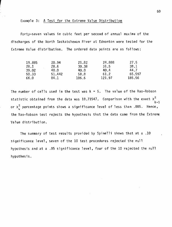
Forty-seven values in cubic fee t per second of annual maxima of the

discharges of the North Saskatchewan River a t Edmonton were tested for the

Extreme Value dis t r ibut ion. The ordered data points are as follows:

The number of c e l l s used in the t e s t was k = 5. The value of the Rao-Robson

s t a t i s t i c obtained from the data was 18.71547. Comparison with the exact x2 k- 1

- or xt percentage points shows a significance level of less than .005. Hence,

the Rao-Robson t e s t re jects the hypothesis tha t the data came from the Extreme

Value dis t r ibut ion.

The summary of t e s t resul ts provided by Spinelli shows tha t a t a .10

significance leve l , seven of the 10 t e s t procedures rejected the nu1 1

hypothesis and a t a .05 significance leve l , four of the 10 rejected the null

hypothesis.

V . MONTE CARL0 POINTS FOR FINITE SAMPLE SIZE

For each of the s i x dis t r ibut ions to which the theory of the Rao-Robson

or Dzhaparidze-Nikulin s t a t i s t i c was applied, Monte Carlo methods were used t o

simulate the percentage points for the t e s t s t a t i s t i c s for f i n i t e sample s izes .

Three different sample s izes were considered, namely n = 20, 50, and 100;

10,000 samples were generated in each case. In a l l instances, equiprobable

ce 1

es t

add

s were formed, and the parameter values were assumed unknown and were

mated by Maximum Density Li kel i hood.

Monte Carlo points for the t e s t s t a t i s t i c s were also simulated for an

tional sample s i ze employing the same number of c e l l s ( fo r example, n=20,

k=4, and n=50, k=4). This generated two points from the same dis t r ibut ion

(namely the Chi-square dis t r ibut ion with k - 1 o r k-s-1 degrees of freedom for

the Rao-Robson and Czhaparidze-Ni kul in s t a t i s t i c s respectively) which together

with the asymptotic dis t r ibut ion point were used f o r the purpose of "smoothing"

the points. The indication in a l l cases was tha t smoothing was not warranted,

and the actual points derived in the main runs were instead l e f t unadjusted. .

For use with the power s tudies , the :Ionte Carlo points were determined

for Pearson's chi-square s t a t i s t i c x2 in the same manner. These points are

included alongside of the associated Rao-Robson or Dzhapardize-Nikulin points

in Tables 1 to 18 following. In addition, the exact asymptotic chi-square

points are provided on the r ight hand s ide of each tab le for comparative

purposes.

In most instances, convergence of the f i n i t e n points to the asymptotic

points appears reasonably rapid. Note, however, t ha t in the case of the

Exponenti a1 d is t r ibut ion , convergence i s comparatively slow with very high

I values s t i l l exis t ing a t n = 100.

You may note tha t there are some c r i t i c a l points tha t do not change from

probability level t o another. This i s due t o the fac t t ha t the Rao-Robson

and Dzhaparidze-Nikulin s t a t i s t i c s are discrete s t a t i s t i c s ; even though the

parameters estimated have continuous d is t r ibut ions , terms in the parameters

cancel out , and the s t a t i s t i c s depend only on the number of observations per

ce l l . Hence, the probability may be concentrated in areas.

TABLE 1

The Normal Distribution

n = 2 0 k = 4

Percentage Points

Pearson Statistic Rao-Robson Statistic

TABLE 2

T h e Normal D i s t r i b u t i o n

P e r c e n t a g e P o i n t s

Pearson S t a t i s t i c Rao-Robson S t a t i s t i c

TABLE 3

The Normal D i s t r i b u t i o n

n = 100 k = 10

Percentage Po in t s

Pearson S t a t i s t i c Rao-Robson S t a t i s t i c

TABLE 4

The E x p o n e n t i a l D i s t r i b u t i o n

n = 2 0 k = 4

Percentage P o i n t s

Pearson S t a t i s t i c Rao-Robson S t a t i s t i c

TABLE 5

The Exponential D i s t r i b u t i o n

Percentage Points

Pearson S t a t i s t i c Rao-Robson S t a t i s t i c

TABLE 6

The Exponential Distribution

Percentage Points

Pearson Statistic Rao-Robson Statistic

TABLE 7

The Double Exponent ia l D i s t r i b u t i o n

n = 2 0 k = . 4

Percentage P o i n t s

Pearson S t a t i s t i c Dzhaparidze-Ni k u l i n S t a t i s t i c

TABLE 8

The Double E x p o n e n t i a l D i s t r i b u t i o n

Percentage P o i n t s

Pearson S t a t i s t i c Dzhapar idze -N i k u l i n S t a t i s t i c

TABLE 9

The Double Exponen t i a l D i s t r i b u t i o n

P e r c e n t a g e P o i n t s

Pearson S t a t i s t i c Dzhaparidze-Ni k u l i n S t a t i s t i c

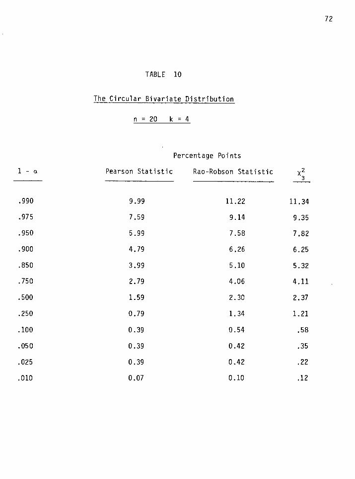
TABLE 10

The Circular Bivariate Distribution

Percentage Poi nts

Pearson S t a t i s t i c Rao-Robson S t a t i s t i c x2 3 -

TABLE 11

The C i r c u l a r B i v a r i a t e D i s t r i b u t i o n

Percentage Po in ts

Pearson S t a t i s t i c Rao-Robson S t a t i s t i c X: -

TABLE 1 2

The C i r c u l a r B i v a r i a t e D i s t r i b u t i o n

n = 100 k = 10

Percen tage Poi n t s

Pearson S t a t i s t i c P.ao-Robson S t a t i s t i c X: -

T A B L E 13

The L o g i s t i c D i s t r i b u t i o n

n = 2 0 k = 4

P e r c e n t a g e P o i n t s

Pearson S t a t i s t i c Rao-Robson S t a t i s t i c

TABLE 14

The Logistic Distribution

Percentage Points

Pearson Statistic Rao-Robson Statistic X; -

TABLE 1 5

The L o g i s t i c D i s t r i b u t i o n

n = 100 k = 10

P e r c e n t a g e P o i n t s

Pearson S t a t i s t i c Rao-Robson S t a t i s t i c

TABLE 16

The Extreme Value Distribution

Percentage Points

Pearson S t a t i s t i c Rao-Robson S t a t i s t i c

TABLE 17

The Extreme Value D i s t r i b u t i o n

Percentage P o i n t s

Pearson S t a t i s t i c Rao-Robson S t a t i s t i c

TABLE 18

The Extreme Value C i s t r i b u t i o n

n = 100 k = 10

Percentage Poi n t s

Pearson S t a t i s t i c Rao-Robson S t a t i s t i c

VI. POWER COMPARISONS

Based on 10,000 samples of s izes 20 and 100, the powers of the Rao-Robson

t e s t s t a t i s t i c (as derived for the f ive dis t r ibut ions previously given) and the

Dzhaparidze-Ni kul in t e s t s t a t i s t i c (as derived for the Double Exponential

dis t r ibut ion) were estimated by Monte Carlo methods. For comparative purposes,

the power of the Pearson t e s t s t a t i s t i c was also simulated. In addition, the

power of t h e Anderson-Darl ing t e s t s t a t i s t i c , A', was detertrined for those

dis t r ibut ions for which the percentage points were avai lahle; reference to some

2 existing power resu l t s for A were also made. The Anderson-Darling s t a t i s t i c

i s based on formulas provided in Stephens (1974, 1977, and 1979). Specifically,

the procedure employed was as follows :

a ) estimate parameters by Maximum Density Likelihood

b) calculate zi = F ( X ~ ; ~ , i=1 ,2 ,...,., n

2 d ) re jec t the null hypothesis i f A exceeds the c r i t i c a l

value for a specified significance leve l .

In a l l cases, a significance level of a = .05 was used. Wherever

possible, the al ternat ive dis t r ibut ions were chosen according t o those

previously employed by others in power simulations (~ormal , Extreme Value,

Exponential). gtherwise, the a l te rna tes were chosen based on the i r general

resemblance to the hypothesized d is t r ibut ion and an attempt t o incorporate a

variety of departures from the nu1 1 dis t r ibut ion (such as skewness, heavy t a i l s ,

broad shoulders , etc . ) .

For a l l sample s izes of n = 20, k = 4 c e l l s were employed; for n = 100,

k = 10 ce l l s were used.

The f i n i t e n c r i t i c a l points for the Rao-Robson and Pearson s t a t i s t i c s

were provided by the Monte Carlo percentage points of the previous chapter.

The f i n i t e n c r i t i c a l points for the Anderson-Darling s t a t i s t i c were

given in Stephens (1974) for the Normal or Exponential d i s t r ibut ions ,

Stephens (1977) for the Extreme Value dis t r ibut ion and Stephens (1979) for the

Logistic dis t r ibut ion. The power comparisons given for in Table 19 were

provided in Stephens (1974).

Dahiya and Gurland produced simulated power resu l t s for the Normal

dis t r ibut ion. For the case where the a l te rna t ive i s the Logistic dis t r ibu-

t ion, t he i r resu l t a t the .05 level of significance a n d for n = 100 i s

direct ly comparable t o tha t obtained for R R . I t i s c lear that the power of the

DG s t a t i s t i c i s f a r superior t o t ha t of the Rao-Robson s t a t i s t i c , a t l eas t in

th i s instance. DG rejected successfully 65.4% of the time versus RR's 10%

success.

In general, fo r small n , the powers of the Rao-Robson a n d Dzhaparidze-

Ni kul in s t a t i s t i c s a re 1 ow, surpassed, where considered, by the EDF Anderson-

Darling s t a t i s t i c . This i s not unexpected given the grouping inherent in chi-

square t e s t s . In cases where the a l te rna t ive dis t r ibut ion i s very close t o the

null dis t r ibut ion (such as in the Normal versus Logistic case above) the

2 improvement of A over RR and x2 i s not s igni f icant , with a l l t e s t s considered

having low power. However, the comparisons performed are relat ively common,

and other, more powerful s t a t i s t i c s (some special ly designed) are readily

appl i cab1 e and therefore preferable.

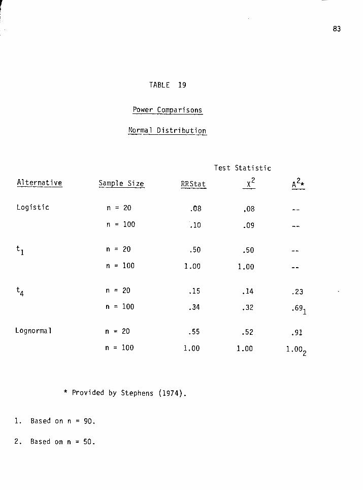
A1 t e r n a t i v -

L o g i s t i c

1

t4

Lognorma 1

TABLE 19

Power Comparisons

Normal D i s t r i b u t i o n

Tes t S t a t i s t i c

Sample S i z e

n = 20

n = 100

n = 20

n = 100

n = 20

n = 100

n = 20

n = 100

RRStat

.08

.10

.50

1 .oo

.15

.34

.55

1.00

* Prov ided by Stephens (1974) .

1. Based on n = 90.

2. Based on n = 50.

A1 t e r n a t i ve

X:

Hal f-Normal

TABLE 20

Power C o m ~ a r i sons

Exponent ia l D i s t r i b u t i o n

T e s t S t a t i s t i c

Sample S i z e RRStat - x2 A --

A1 t e r n a t i v e

L o g i s t i c

TABLE 2 1

Power Comparisons

Doub le E x p o n e n t i a l D i s t r i b u t i o n

Sample S i z e

T e s t S t a t i s t i c

DNStat x -

A 1 ternative

Uniform

Bivariate Normal

TABLE 22

Power Comparisons

Circular Bivariate Distribution

Test Sta t i s t ic

Sample Size RRSta t

TABLE 23

Power Comparisons

L o g i s t i c D i s t r i b u t i o n

T e s t S t a t i s t i c

A1 t e r n a t i v e Sample S i z e RRStat x - A -

Normal

TABLE 24

Power Compar isons

Extreme V a l u e D i s t r i b u t i o n

Sample S i z e RRStat

8 8

A1 t e r n a t i v e

Be ta (1,4)

T e s t S t a t i s t i c

VII. CONCLUSIONS

Clearly, there has been a good deal of attention centred on chi-square

goodness-of-fit techniques, and in t e res t in the area i s continuing. As

long as the ve r sa t i l i t y and ease of computation are retained, developing 2

improvements t o Pearson's t e s t s t a t i s t i c X i s a worthwhile endeavour.

The review of some of the modern methods indicates the areas into

which in teres t has evolved, namely in overcoming the handicaps of Pearson's

t e s t by producing a1 ternate quadratic forms, by adapting a chi -square t e s t

t o other than fu l l sample data where competitive procedures are unavai 1 able,

and by ta i lor ing a chi-square t e s t t o , fo r example, a mu1 t iva r i a t e d i s t r i -

bution where, again, other t e s t s are not applicable. There i s a wide area

open fo r future study.

The resu l t s of the previous sections indicate tha t implementation of

the Rao-Robson (or Dzhaparidze-Nikulin in cases where R R i s undefined) 2 s t a t i s t i c in favour of X i s recommended. The obvious advantage i s tha t the .

asymptotic dis t r ibut ion i s exactly tha t of chi-square, and the convergence

of the f i n i t e n percentage points i s rapid enough to jus t i fy i t s use; par t i -

cularly fo r small values of k , there i s potent ial ly large e r ro r inherent in 2

the X t e s t when the MDL estimates are used. The disadvantage of the new

t e s t procedures i s the necessity of deriving the part icular form of the

s t a t i s t i c for each hypothesized d is t r ibut ion . This, as shown, i s usually

not d i f f i cu l t . For some spec i f ic d is t r ibut ions , such as the Beta dis t r ibut ion,

the integrals involved must be solved numerically for the Rao-Robson s t a t i s t i c ,

b u t in many cases, the derivation i s qui te simple.

As f a r as the general application of chi-square t e s t s i s concerned, i t i s

s t i l l recommended tha t , where the conditions of the t e s t allow, more powerful

s t a t i s t i c s such as the EDF s t a t i s t i c s be used. To emphasize a frequently

made point, the basis for preference of a chi-square t e s t remains to be

i t s wi de-spread appl i cabi 1 i t y and ease of cal cul a t i on.

A P P E N D I X

9 2 i . S u b r o u t i n e f o r Normal D i s t r i b u t i o n I . . . . . . . . . . . . . . . . I

. . . . . . . . . . . . . i i . Subrou t ine f o r Exponent ia l D i s t r i b u t i o n 95

i i i . S u b r o u t i n e f o r Double Exponent ia l D i s t r i b u t i o n . . . . . . . . . . 97

i v . S u b r o u t i n e f o r C i r c u l a r B i v a r i a t e D i s t r i b u t i o n . . . . . . . . . . 100

v. Subrou t ine f o r L o g i s t i c D i s t r i b u t i o n 103 ! . . . . . . . . . . . . . . . I I I

v i . Subrou t ine f o r Extreme Value D i s t r i b u t i o n . . . . . . . . . . . . 108 I

9 2 i . Su h r o u t i ne RRI!ORM

T H I S SUBROUTINE TAKES THE IRPUT DATA X ARD CALCULATES THE RAO ROBSON S T A T I S T I C RRSTAT. ASSUMING WE WISH TO TEST FOR NORMALITY, N I S THE b!O. OF DATA POINTS ARD K I S Tt!E NUHBER OF CELLS.

SUEROUTINE RRI\!ORM(X ,I\!, K,RRSTAT) INTEGEF? OSS(K) ,F.!Ufl(K) D IRENSION C ( K ) ,D(K,2) ,BOUND(K) DIMENSION X(N) ,D IFF(N) ,A(2,2),V(K,2)

REQUIRE ONE X ( 1 ) I N ASCENDING ORDER

CALL VSRTA ( X ,N)

CALCULATE THE PARAMETER ESTIKATES

SUM1 =O .O XN=N DO 1 I = l , N SUM1 =SUH1 +X ( I ) TH l=SUMl /XN SUM2=0 .O DO 2 I = l , N DIFF(I)=X(I)-TH~ SUM~=SU~I~+(DI FF( I ) * D I F F ( I)) T H ~ = s Q R T ( S U ~ I ~ / ( X N - ~ .O))

THE K+I CLASS BOUKDARIES ARE OF THE FORK T H ~ + C ( 1 1 ~ ~ 2 . WE CAN O B T A I N THE C ( 1 ) ' S E A S I L Y FROM THE STANDARD NORHAL TAPLE. THE FOLLOWING ARE GIVEN FOR K=10.

FOR K=4, THE ~ ( 1 ) ' s ARE:

CALCULATE THE BOUNDARIES.

TO DETERMINE THE NUMBER OF OBSERVATIONS PER CELL, FIRST CALCULATE THE NUMBER OF OBSERVATIONS LESS THAN OR EQUAL TO EOUND(1) ,I=l,M

IS=1 DO 4 J=l,K TEMP=BOUMD(J) DO 5 I=IS,N IF(X(I).GT.TEMP) GO TO 50 CONTIRUE IF((I .EQ.N).AND. (X(I).LT.TEMP)) GO TO 51 NUM(J)=I-1 IS=I GO TO 4 NUM(J)=N IS=M CONTINUE

NOk CALCULATE THE KUYBER OF~OBSERVATIOMS PER CELL.

DETERMINE THE D(I)'s, V(I)IS, AND A(I,J)IS REQUIRED TO CALCULATE THE TEST STATISTIC.

XN=N XK=K E(l,l)=0.0 Ql=SQRT(2.0*3 .l4l6) DO 7 I=2,K Q2=-(C(1-l)*C(I-1)/2.0) Q3=- (C(I)*C(I)/Z.O) D(I,l)=(l .O/(TH~*(Q~)))*(EXP(Q~)-EXP(Q3)) CONTINUE D(~,~)=(~.o/(~.o*TH~*TH~*Q~))*(-c(~)*ExP(Q~)) DO 9 I=2,K D(1,2)=(1 .o/(~.o*TH~*TH~*Q~))*(c (I-~)*ExP(Q~)-C(I)*EXP(Q3) CONTINUE DO 10 I=l,K V(IS1)=TH2*D(I,1) v(I,2)=TH2*TH2*D(IY2) CONT I NUE

THE A(1,J)'S ARE THE ENTRIES OF THE !,!ATRIX (v+ - J)+ OHERE + C DENOTES INVERSE.

SUM3=O .O DO 11 I = l , K S U M ~ = S U ~ ! ~ + V ( I , 2 ) * V ( I ,2) SUM4=O .O SUF15 =O . 0 DO 1 2 I = l , K SUM4=SUM4+V(I , 1 ) * V ( I , 2 ) S U M ~ = S U M ~ + V (I , l ) * V ( I ,1) CONTINUE Q ~ = ( X K * S U M ~ - 1 . 0)* (xK*SUY3-2.0) - (XK*X K * S U Y ~ * S U M ~ )

READY TO CALCULATE A ( 1 , J ) ' S.

S'JY6=0 .O SUr47=0 .O SUM8 =O . 0 XNK=XN/XK DO 1 4 I = l , K XOBS=OBS( I ) SU!46=SUM6+(XO!3S-XNK)* (XOES-XNK) SUM~=SUM~+((XOBS-XNK)*V(I ,I)) S U ! ~ ~ = S U K ~ + ( (XOBS-XNK)*V ( I ,2) ) CONTINUE

READY TO CALCULATE THE RAO-ROBSON S T A T I S T I C .

RRSTAT=XKN*SU%~+XKN*XK*Q~*A (1 ,1)+2 .O*XKN*XK*Q~*A (1 , ~ ) + x K ~ ! * X K * Q ~ * A ( ~ ,2) RETURN END

i i . S u b r o u t i n e RREXP

T H I S SUBROUTINE TAKES THE INPUT DATA X AND CALCULATES THE RAO ROBSON S T A T I S T I C RRSTAT. ASSU?!ING WE WISH TO TEST FOR EXPOMENTIALITY, N I S THE NO. OF DATA POINTS AND K I S THE NUMBER O F CELLS.

SUBROUTINE RREXP(X,M ,K,RRSTAT) INTEGER OBS(K ) , NUH(K) D IMENSION C ( K ) .D ( K ) . v ( K ) ,BOuRD(K) D I H E N S I O N X ( N )

WANT X ( 1 ) I N ASCENDING ORDER

CALL VSRTA (X ,N)

CALCULATE THE PARAMETER ESTIMATES

SUM1 =O .O XN=N XK=K DO 1 I = l , N sur.11 =S~l11+:: ( I ) CONTINUE T H l = S U ! f l / X N

THE K+1 CLASS BOUNDARIES ARE OF THE FORK X B , ~ R * C ( I - 1 )

CZERO=O.O C ( K ) = 9 9 9 9 9 9 . 0 KK=K-1 DO 2 I = l , K K X I = I c ( I ) = - A L O G ( ~ .o- (XIIXK)) CONTINUE CALCULATE THE D ( I ) ' S : ~ ( i ) = ( i .OITHI)*~-c(~)*ExP(-~(1))) DO 3 I = 2 , K D(I)=(l.O/T~1)*(C(I-l)*EXP(-C(I-1))-C(I)*EXP(-C(I))) CONTINUE CALCULATE THE V ( I) ' S : DO 4 I = l , K V(I)=THI*D(I) CONTINUE DETERMINE THE BOUNDARIES, BDZERO=O .O DO 5 I = l , K BOUND(I)=TH~*C ( I) CONTINUE DETERMINE THE NUMBER OF OBS. LESS THAN BOUND(J) I S = l DO 6 J = l , K TEMP=BOUND (J)

9 6

DO 7 I = I S , N IF(X(I).GT.TEMP) GO TO 50

7 CONTINUE IF((I.EQ.N).AND.(X(I).LT.TEMP)) GO TO 5 1

50 NUM(J)=I-1

GO TO 6 5 1 NUM(J)=N

6 CONTINUE DETERMINE THE NUMBER OF oes. IN EACH CELL O B S ( ~ ) = N U H ( ~ ) DO 8 I=2 ,K OBS(I)=NUM(I)-NU?:(I-1)

8 CONTINUE READY TO CALCULATE THE RAO-ROBSON S T A T I S T I C SUMZ=O. 0 SUM3=0 .O SUF?4=0.0 XNK=XN/XK DO 9 I = l , K

I- XOBS=OBS ( I ) I SUMZ=SUMZ+(XOBS-XtYK)* (XOBS-XNK)

S U M ~ = S U Y ~ + ( ( X O B S - X N K ) * V ( I))* ((XOBS-XNK)*V (I)) k SUH4=SUPl4+V ( I )*V ( I ) r 9 CONTINUE

XKN=XK/XN C

RRSTAT=XKN*SU?~~+(XK*XKN)* (SUM31 (1.0-XK*SUM4)) RETURF! END

iii. S u b r o u t i n e DNDEXP

T H I S SUBROUTINE TAKES THE INPUT DATA X AND CALCULATES THE DZHAPARIDZE-NIKULIN S T A T I S T I C TO TEST FOR DOUBLE EXPONENTIALITY. N I S THE NO. OF DATA POINTS AND K I S THE NUb?EER OF CELLS.

SUBROUTINE DNDEXP ( X ,PI, K,DNSTAT) DIMENSION D I F F ( N ) ,X(N) ,C(K) ,D(K) ,BOUND(K),XOBS(K) INTEGER OBS(K) ,NUM(K)

K MUST BE CHOSEN AS EVEN FOR THE FOLLOKING:

WANT THE DATA POINTS I N ASCENDING ORDER:

CALL VSkTA ( X ,N)

NON CALCULATE THE PARAMETER ESTIMATES:

I F N I S ODD, T H 1 I S X (N+1) /2 . OTHERWISE, TW1 I S ( x ( N / z ) + x ( N / z + ~ ) ) / ~ .

I F N I S EVEN, USE:

I F N I S ODD, USE:

CELL BOUNDARIES ARE CHOSEN SUCH THAT P ( I ) = l / K . THE I T H BOUNDARY I S TH1+ OR -C(I)THZ. NOK F I N D THE C ( I ) , SETTING CZERO AND C (NU) SEPARATELY.

N U U = N U = l X N U = N U DO 2 I=l,NUU XI=I C(I)=-ALOG(l.0-(XIIXNU)) CONTINUE

NOW CALCULATE THE D(1) 'S:

D ( I ) = - c ( ~ > * E x P ( - c ( ~ ) ) SUtl2=D (l)*D ( 1 ) DO 3 I=2,NU D(I)=c(I-I)*EXP(-C(I-1))-C(I)*EXP(-~(1)) SUFZ=SUM2+D (I)*D( I ) CONTINUE

NOW CALCULATE THE EOUNDARIES:

EDZERO=-999999.0 B O U N C ( N U ) =THI ; DO 4 I=lyNU E O U N D ( N U + I ) = T H ~ + C ( I ) * T H ~ DO 5 I=1 y N U U BOUNC(NU- I)=THI-c (I)*THZ

NO\! CALCULATE THE NO. O F OBSERVATIONS LESS T H A N OR EQUAL TO BOUND ( J) . IS=1 DO 6 J= l ,K TEF?P=EOUND ( J ) DO 7 I=IS,N I F ( X ( I ) .GT.TEMP) GO TO 50 CONTINUE IF ( ( I .EQ.N) . A N D . ( X ( I ) . L T . T E W ) ) GO TO 51 NUN(J)=I-1 IS=I GO TO 6 NUM(J)=N IS=N CONTINUE

NOW CALCULATE THE NUFIEER OF OBSERVATIONS PE!? C E L L :

OBS(~)=NU!I (1 ) DO 8 I=2,K OBS(I )=NUY(I) -NUM(I-1) CONTINUE

R E A D Y TO CALCULATE THE STATISTIC.

SUr:2 IS CALCULATED AEOVE. SUM3 RUMS FROM 1 TO N . BUT SU!I4 FROM 1 TO N U , SO DETERMINED SEPARATELY.

C sur13=0 . 0 SUM4=O. 0 XNK=XN/XK DO 9 I = l , K XOBS ( I ) =OBS ( I ) S U Y ~ = S U M ~ + ( X O B S ( I)-XNK)* (XOBS(1)-XF!K)

9 CONTINUE DO 11 I = l , N U XOBS(I)=OBS(I) S U I I ~ = S U M ~ + D ( I)* (XOBS(NU+I)+XOBS(NU-I+1) )

11 CONTINUE SUM4=SUM4*SUM4 XKN=X K/XN

C C CALCULATE THE D-N S T A T I S T I C . C

DNSTAT=XKNkSUH3- (XKN/ ( 2 .O*SUM2) )*SUM4 RETURN END

i v . S u b r o u t i n e RRCB

T H I S SUBROUTINE TAKES THE I N P U T DATA X AND CALCULATES THE RAO ROESON S T A T I S T I C RRSTAT TO TEST FOR THE CIRCULAR B I V A R I A T E D I S T R I B U T I O N . N I S THE NO. OF DATA POINTS AND K I S THE NO. OF CELLS .

SUBROUTINE RRCB(X,Y ,N,K,RRSTAT) INTEGER O B S ( K ) ,NUM(K) D I R E N S I O N C ( K ) ,C(K) ,V(K) ,BOUND(K) , X ( N ) D IMENSION Y ( N ) , D I F F ( ~ N ) ,RADIUS(N)

PLACE DATA I N ASCENDING ORDER

CALCULATE THE THREE PARAMETER ESTIMATES. XN=N X K=K SUM1 =O . 0 SUM2=O .O SUM3=O .O sut.14=0.0 DO 1 I = l , N S U M ~ = S U M ~ + X ( I ) SuM2=SUMZ+Y ( I ) CONTINUE T H I = S U M l / X N TH2=SUM2/XN DO 2 I = l , N SUM~=SUM~+(X(I)-THl)*(X(I)-TH1) SUI.I~=SU~M+(Y( 11-THZ)*(Y ( I 1-THZ) CONTINUE T H ~ = ( s u ~ ~ ~ + S U N ~ ) / ( 2 .*XN) T H ~ = S Q R T ( T H ~ )

CELLS ARE CENTRED A T (XBAR,YBAR) WITH SUCCESSIVE R A D I I C ( I ) T H 3 , F I R S T REQUIRE THE C ( 1 ) ' S .

CZERO=O .O KK=K-1 DO 3 I = l , K K X 1=1 C ( I ) = S Q R T ( - ~ . O * A L O G ( ~ . 0 - ( X I / X K ) ) ) CONTINUE C ( K ) = 9 9 9 9 9 9 . 0 V ( 1 ) = - (C ( l ) * C ( l ) ) * ( E x P ( - . 5 * ( c ( l ) * c ( l ) ) ) ) DO 4 I = 2 , K K QTYl=(C(I-l)*C(I-l))*(EXP(- . 5 * ( ~ ( 1 - 1 ) * ~ ( 1 - 1 ) ) ) ) QTY2=(C(I)*C(I))*(EXP(-.~*(C(I)*C(~)))) V(I)=QTY~-QTYZ CONTINUE

DO 5 I=l,K D(I)=V (I)/2.0 CONTINUE

FIND THE BOUNDARIES BY DETERMINING THE RADII C(I)TH3.

DO 6 I=l,K BOUND(I)=C(I)*TH~ CONTINUE

IF THE DISTANCE FROM (XBAR,YBAR) TO (~(1) ,Y(I)) IS LESS THAN RADIUS(1) THEN THE NUMBER OF OBS. IN CELL(I) INCREASES BY ONE. ALTERb!ATIVELY, KE CAN CALCULATE ALL THE DISTANCES (XBAR,YBAR) TO (~(1) ,Y(I)) AND THEN FIND THE NUMBER LESS THAN RADIUS(I).

DO 7 I=l,N DIFF(I)=X(I)=TH~ NN=N+I DIFF(NN)=Y(I)-THE IF(DIFF(I) .LT.O.O) DIFF(I)=DIFF(I)*(-1 .o) IF(DIFF(NN) .LT.O.O) DIFF(~!N)=CIFF(NP!)*(-1 .o) CONTINUE NN=2*N DO 8 I=l,N RADIUS(I)=SQRT((DIFF( I)*DIFF(I))+DIFF(N+I)*DIFF(N+~))) CONTINUE CALL VSRTA (RADIUS,N)

FIRST REQUIRE THAT THE DISTANCES FROM XBAR,YBAR BE IN ASCENDING ORDER.

IS=l DO 9 J=l,K TEMP=BOUND (J) DO 1 0 I=IS,N IF (RADIUS(I).GT.TEMP) GO TO 50 CONTINUE IF((I.EQ.N).AND.(RADIUS(I).LT.TEMP)) GO TO 51 NUI"I(J)=I-1

GO TO 9 NUM(J)=N IS=N CONTINUE

NOW CAN F IND THE NUMEER OF OBS. PER CELL.

O B S ( ~ ) = N U M ( ~ ) DO 11 I=2,K OES(I)=NUM(I)-NUM(I-1) CONTINUE FORMAT ( / 2 X , 5 1 1 0 )

READY TO CALCULATE THE RAO-ROBSON S T A T I S T I C .

SUM5 =O .O SUM6=O. 0 SUM7 =O .O XNK=XN/XK DO 1 2 I = l , K XOBS=OBS( I) SU~ . I~=SUY~+(XOBS-XNK) * (XOBS-XNK) SUI:~=SUM~+XOBS*D (I ) S U H ~ = S U F . ~ ~ + ( D ( I ) * D ( I ) ) CONTINUE XKN=XK/XN

RRSTAT=XKN*SUM~+(XK*XKN* (SuN6*Sur46))/ (1 .O-XK*SU!l7) RETURN END

v . S u b r o u t i n e RRLOG

T H I S SUEROUTINE TAKES THE INPUT DATA X AND CALCULATES THE RAO ROBSON S T A T I S T I C RRSTAT. TO TEST FOR THE LOGIST IC D I S T R I E U T I O N N I S THE NO. OF DATA POINTS AND K I S THE NUMBER OF CELLS.

SUBROUTINE RRLOG(X,N.K,RRSTAT) DIMENSION C ( K ) ,D(K,2) ,V(K,Z),A(2,2) ,Q(K) DIMENSION X(N) ,Z(N) INTEGER OBS(K) ,MUM(K)

REQUIRE X ( 1 ) I N ASCENDING ORDER:

CALL VSRTA (X ,N)

CALCULATE THE PARAKETER ESTIMATES:

F IRST CONSIDER THE CASE b!HERE BOTH PARAMETERS ARE UNKNOWN. THE KEAN AKD STAb!DARD DEVIAT ION*P I /SQRT3 W I L L BE THE I N I T I A L USED I N THE I T E R A T I V E NUMERICAL SOLUTION:

XN=N XK=K SUM1 =O .O SUM2=0.0 DO 1 I = l , N SUt41=SU!?l+X(I) CONTINUE THl=SU:41/XM DO 2 I = l , N SU~~I~=SU~I~+(X( I 1-TH~) * ( x ( I 1 - T H ~ ) CONTINUE STD=SQRT (SUN2/XN) P I = 3 . 1 4 1 5 9 2 6 5 T H ~ = ( P I / s Q R T ( ~ . O ) ) * S T D TH2=STD

BEGIN THE I T E R A T I V E PROCESS TO F I N D TH1,THZ:

COUNT=O .O COUNT=COUNT+l .0 CALL FUMS(X ,N,THl ,TH2,FXY ,GXY) CALL DERIV(X ,NYTH1 ,TH2,FPX ,FPY ,GPX ,GPY) XS=( (GXY*FPY) - (FXY'GPY) ) I( (FPX*GPY) - (FPY*GPX) ) YS=((GXY*FPX)- (FXY*FPX) ) / ( (FPY*GPX) - (FPX*GPY)) TH lS=TH l+XS TH2S=TH2+YS DIF~=ABS(XS) DIFZ=AES(YS) I F (COUMT.GT.~O.) GO TO 5 2 IF ((DIF~.LT..OOO~).AND.(DIF~.LT..OOO~)) GO TO 50 T H l = T H l S

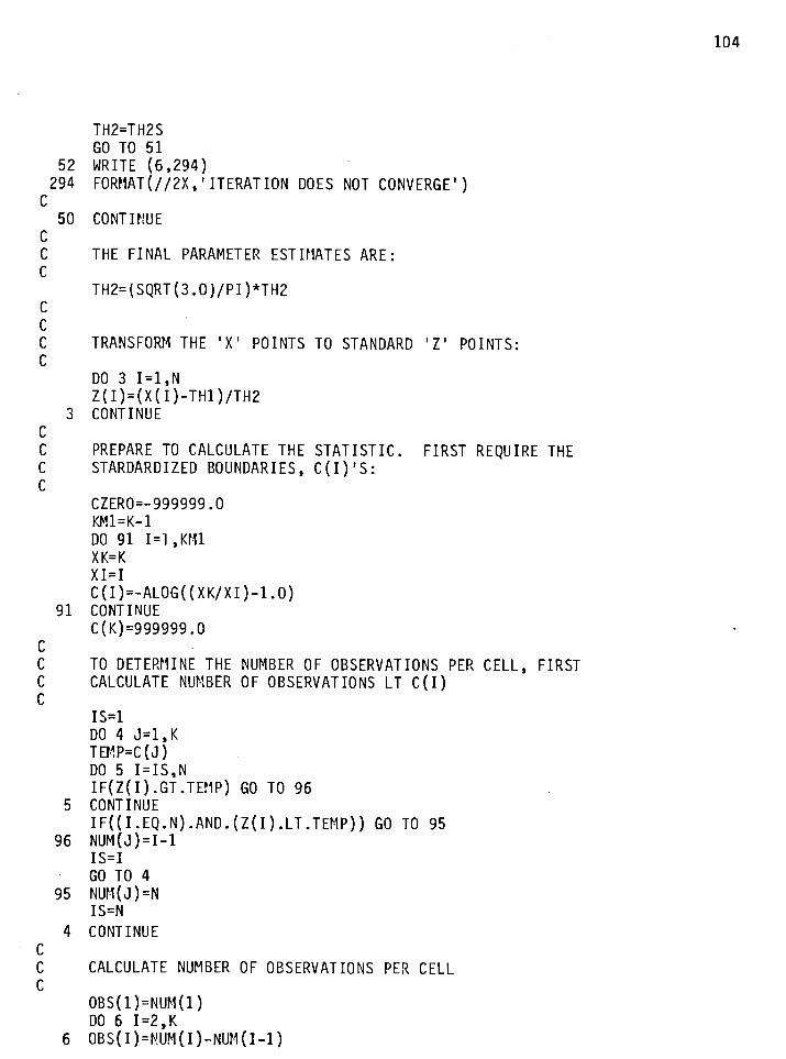
TH2=TH2S GO TO 5 1 WRITE (6 ,294 ) FORHAT(//ZX, ITERATION DOES NOT CONVERGE' )

THE F I N A L PARAMETER EST IHATES ARE :

TRANSFORM THE ' X I POINTS TO STANDARD ' Z ' POINTS:

DO 3 I = l , N z(I)=(x(I)-THI)/THZ CONTINUE

PREPARE TO CALCULATE THE S T A T I S T I C . F I R S T REQUIRE THE STARDARDIZED BOUNDARIES, C (I) ' S :

CZERO=-999999.0 KF-il=K-1 DO 9 1 1=1 ,KM1 XK=K X I = I c(I)=-ALOG((XK/XI)-1.0) CONTINUE C(K)=999999 .0

TO DETERrlINE THE NUMBER OF OBSERVATIONS PER CELL, F IRST CALCULATE NUNBER OF OESERVATIONS L T C (I)

I S = l DO 4 J= l ,K TEt{P=C (J) DO 5 I = I S , N IF(Z(I).GT.TE!IP) GO TO 9 6 CONTINUE IF((I .EQ.N) .AND. (z(I) .LT.TEMP)) GO TO 9 5 NUM(J)=I-1 I S = I GO TO 4 NUM(J)=N IS=N CONTINUE

CALCULATE NUMBER OF OESERVATIONS PER CELL

1

C C DETERMIIJE D(I , J ) ' S (HAVE STANDARD Z POINTS AND PARAYETERS TH1, T H 2 ) C

DO 7 I = l , K M l Q(I)=EXP(-C(I))/((l.O+EXP(-C(I)))**2)

7 CONTINJE H l l = K - 1 D ( l , l ) = - Q ( l ) D ( 1 , 2 ) = - C ( l ) * Q ( l ) D ( K , ~ ) = Q ( K F ? ~ ) D(K,2)=C (W41)*C( ICm~l l ) DO 7 7 I=2,KM1 D ( I , l ) = ( Q ( I - l ) - Q ( I ) ) D(I,2)=-C(I)*Q(I)+C(I-l)*Q(I-1)

7 7 CONTINUE C c DETERMINE A( I , J ) 'S C

SUF? 1 =o . 0 SUM2=O .O SU113=0.0 DO 8 I = l , K S U M ~ = S U M ~ + D ( I , ~ ) * D ( I , ~ ) SUtl2=SUM2 + D ( I , 2 ) * D ( I ,2) SUY3=SUM3 + D ( I , l ) * ~ ( 1 , 2 )

8 CONTINUE P I = 3 . 1 4 1 5 9 2 6 5 3 6 G l = ( 3 .O+P I * *2 ) / 9 .O DDz(G1-XK*SUM2)* (1 .O/3 .O-XK*SUYl ) - ( (XK*SUN3)**2 ) CC=l.ODO/DD

C A ( 1 , l )=cC*(G l -XK 'SuM2) A ( l , ~ ) = C C * X K * S U M ~ A (2 ,1 )=A (1 ,2 ) A(2,2)=CC*(1.0/3.0-XK*SuM1)

C C READY TO CALCULATE RRSTAT C

SUM4=O. 0 SU!15=0.0 SUF16=0.0 XNK=XN/XK XKN=X K/XN DO 9 I = l , K XOBS=OBS ( I ) s u r l 4 = s u n 4 + ( x o ~ s - x NK)* ( x o ~ s - X N K ) S U ~ = S U M ~ + (XOES-XNK)*D(I ,I) SU!?6=SUM6 + (XOBS-XNK)*D ( I ,2)

9 CONTINUE Q5 =SU?l5*SUM5 Q6=SUR6*SU:16 Q7=SU!15*SUM6

SUBROUTINE TO CALCULATE THE VALUES OF F(A,B) AND G(A,B): SUBROUTINE FUNS(X ,N,A,E,FXY ,GXY) DIMENSION x ( N ) XN=N SUM1 =O . 0 su:12=0.0 P I = 3 . 1 4 1 5 9 2 6 5 DO 100 I = l , N C=EXP((PI*(X(I)-A))/(B*SQRT(3.))) D = l . / ( l . + C ) SUMl=SUMl+D E = ( l . - C ) / ( l . + C ) F=(x(I)-A)/B DZ=E*F SUMZ=SUMZ+DZ CONT INUE FXY=SUfl1/XN GXY=SUMZ/XPI FXYzFXY- .5 GXY=FXY+(SQRT(3. ) / P I ) RETURN END

SUBROUTINE TO CALCULATE THE DERIVATIVES OF F(A,B) AND G(A,B) : SUBROUTINE DERIV(X,N,A,B,FPX,FPY,GPX,GPY) D IRENS I O N x (N ) P I = 3 . 1 4 1 5 9 2 6 5 CON=PI/ (SQRT(3. ) * B ) XN=N Su!:1 =o . 0 sur12=0.0 SUMlA=O. 0 SU?;ZA=O. 0 DO 100 I = l , N K=DONf(X ( I ) -A) EW=EXP(W) SUMl=SUMl+EW/ (1 .+EW)**2 DWDE=DON*((A/B)- (X ( I ) / B ) ) SUMlA=SUMlA+(EW/ (1. +EW)**Z)*DWDE Pl=W-W*EW P Z = l . / (1. + E W ) * * ~ P3=1. -K*EW-EW P 4 = l . / (1. +EW) PROD=-1 .*Pl*PZ*EW+P3*P4 SUMZ=SUEZ+PROD SUMZA=SUEZA+(PROD*DWDB) CONTINUE FPX=(CON/XN)*SUMI FPY=SUM~A/XN* ( -1 . ) GPX=SUMZ*(-I. / (B*XN) )

G P Y = S U M ~ A * ( S Q R T ( ~ . ) / ( X N * P I ) ) RETURN END

v i . S u b r o u t i n e RREVD

T H I S SUBROUTINE TAKES THE INPUT DATA X AND CALCULATES THE RAO ROBSON S T A T I S T I C RRSTAT. TO TEST FOR THE EXTREME VALUE D I S T R I B U T I O N N I S THE NO. OF DATA POINTS AND K I S THE NUMBER OF CELLS.

SUBROUTIb!E RREVD ( X ,N, K,RRSTAT ,PEAR ,TH1 ,TH2) DIMENSION X(N) ,xX(N) ,Z(N) DIMENSION C ( K ) , D ( K , ~ ) ,A(2,2) DIMENSION Q ( K ) INTEGER OBS(K) ,NuM(K)

REQUIRE X ( 1 ) I N ASCENDING ORDER

CALL VSRTA (X ,N)

CALCULATE THE PARAMETER ESTIMATES.

VAR=O .O SUM=O .O XN=N DO 3 3 I = l , N SUM=SUF + X ( 1 ) CONT I NU E THl=SUM/XN DO 2 2 I = l , N XX(I)=X(I)-THI VAR=VAR+(XX (I)*XX (I)) CONTINUE STD=SQRT(VAR/ (XN-1 .o) ) TH2=STD/ 1 . 3 CALL THETA(X ,N,TH2) CALL Z I (X ,NYTH2,TH l )

STANDARDIZE THE X VALUES: Z = ( X - T H l ) / T H 2

DO 1 I = l , N Z ( I ) = ( x ( I ) - T H l ) / T H E CONTINUE

REQUIRE STANDARDIZED CELL BOUNDARIES C (I) ' S

CZERO=-999999.0 K r l l = K - 1 DO 2 I = l , K M l X I = I XK=K c(I)+-ALOG(-ALOG(XI/XK)) CONTINUE C(K) = 9 9 9 9 9 9 . 0

TO DETERMINE THE NUMBER OF OBSERVATIONS PER CELL, F IRST TO CALCULATE THE NUYBER OF OBSERVATION L T C ( 1 )

I S = l DO 4 J = l , K TEMP=C (J) DO 5 I = I S , N IF(Z(I).GT.TEMP) GO TO 50 CONTINUE IF((I.EQ.N).AND.(Z(I).LT.TEMP)) GC TO 5 1 NUM(J)=I-1 I S = I GO TO 4 NUH ( J ) =N I S = N CONTINUE

NOW CALCULATE THE NUMBER OF OBSERVATIONS PER CELL

DETERVINE D ( I ,J)' S. HAVE STANDARDIZED DATA POINTS AND PARAMETERS T H 1 AND TH2.

Q(K)=O.O DO 7 I = l , K N l Q ( I )=EXP( -~ (1 ) -EXP( -~ (1 ) ) ) CONTINUE D ( 1 , l ) = - Q ( l ) D ( 1 , 2 ) = - C ( l ) * Q ( l ) D ( K , l ) = Q ( K W D ( K , ~ ) = c ( K M ~ ) * Q ( K M ~ ) DO 7 7 1=2,KM1 D ( I , l ) = Q ( I - l ) - Q ( I ) D(I ,z)=c(I-I)*Q(I-1)-c(I)*Q(I) CONTINUE

PREPARE TO CALCULATE A ( I ,J) ' S :

EC= .577215664 P I = 3 . 1 4 1 5 9 2 6 5 3 6 SUMl=O.O SUM2=O. 0 SUM3=O. 0 DO 8 I = l , K SUMI=SUH~ + D( I ,~ ) *D( I ,~ ) SUM2=SUM2 + D( I , 2 ) * D ( I ,2) SUM3=SUM3 + D ( I , l ) * D ( I , 2 ) CONT I b!U E C l = P I * P I / 6 . 0

PREPARE TO CALCULATE THE IFPUTS FOR RRSTAT

SUF?4=0.0 sut!i5=0 .o SUM6=O. 0 XNK=XN/XK XKN=XK/XN DO 9 I = l , K XOES=OBS ( I) SUM4=SUf44 + (XOBS-XNK)* (XOBS-xNK) SUM5=SUM5 + ( (XOBS-XNK)*D (I ,I)) SUM6=SUM6 + ( (XOBS-XNK)*D( I ,2) ) CONTINUE Q5=SUM5*SUM5 Q6=SUt16*SUt16 Q7=SUM5*SUM6

READY TO CALCULATE RRSTAT:

RRSTAT=XKN*SUM4+XKN*XK*Q5*A(lSl)+2 . O * X K * X K N * Q ~ * A ( ~ ,2) + X K N * X K * Q ~ * A ( ~ ,2) RETURN END

SUBROUTINE THETA ( X ,N ,TI DIMENSION X(N) WRITE(^ ,100) F0RKAT(7X, 'T1 , 1 l X , ' T I ' ,5X, 'COUNT' ) wRITE(6,ZOO) S1=0 .o COUNT=O .O IF (T .GT .1 .8 ) T=T/1 .5 DO 1 0 I = l , N S l = S l + X ( I ) CONTINUE S l = S l / N S2=0 .o S3=0.0

COUNT=COUNT+l .0 DO 2 0 I = l , N E=EXP(-x(I)/T) S2=S2+X ( I )*E S3=S3+E CONTINUE T l = S l - S 2 / S 3 WRITE (6 ,200 ) T , T I ,COUNT T l = ( ~ + T 1 * 2 . 0 ) / 3 . 0 FORMAT (2X , 3 F l 2 . 6 ) Z=ABS(T-TI) T=T1 IF (COUNT.GT.~O.O) GO TO 3 1 I F ( Z . L T . 0 . 0 0 1 ) GO TO 3 0 GO TO 1 5 CONTINUE WRITE ( 6 , 3 0 0 ) T FORMAT(/ZX, IT = ' , ~ 1 2 . 6 ) RETURN T=1.0 WRITE ( 6 , 7 0 0 ) FORRAT ( / 2 X , ' ITERATION D I D NOT CONVERGE' ) RETURN END

SUBROUTINE Z I (X ,N,T,Z) DIMENSION X(N) S=O. 0 DO 1 0 I = l , N S=S+EXP(-X(I )/TI CONTINUE z=-T*ALOG(S/N) WRITE ( 6 , 1 0 0 ) Z FORt IAT(2X, 'Z I= ' ,F12.6) RETURN ENE

BIBLIOGRAPHY

Andrews, D.F., Gnanadesikan, R . and Warner, J.L. (1973) . "Methods f o r A s s e s s i n g Mu1 t i v a r i a t e Normal i ty" i n Mu1 t i v a r i a t e A n a l y s i s I 1 1 (P.R. K r i s h n a i a h , E d i t o r ) . New York: Academic P r e s s , 95-116.

Barankin , E . D . and Gurl a n d , J . (1951) . "On A s y m p t o t i c a l l y Normal E f f i c i e n t E s t i m a t o r s ." Univ. C a l i f . Pub1 . S t a t 1, 89-129.

Chernoff , H . and Lehmann, E .L . ( 1 9 5 4 ) . "The Use o f Maximum-Like1 ihood Es t imates i n Chi-Square T e s t o f Goodness o f F i t . " The Annals of Mathematical S t a t i s t i c s , 25, 579-586.

Cochran, Wil l iam G . (1952) . "The Chi-Square T e s t o f Goodness o f F i t . " The Annals of Mathematical S t a t i s t i c s , 23 , 315-345.

Cochran, Will iam G . ( 1 9 5 4 ) . "Some Methods f o r S t r e n g t h e n i ~ g t h e Common Chi-Square T e s t s . " Biometries, 1 2 , 417-451.

Dahiya, Ram. C . and Gur land , John. (1972a) . "Pearson Chi-Square T e s t o f F i t w i t h Random I n t e r v a l s . " B i o m e t r i k a , 5 9 , 147-153.

Dahiya, Ram. C . and Gur land , John. ( l 9 7 2 b ) . "A T e s t o f F i t f o r Continuous D i s t r i b u t i o n s Based on G e n e r a l i z e d Minimum Chi-Square ." i n S t a t i s t i c a l Papers i n Honor of George W . Snedecor (T.A. B a n c r o f t , e d i t o r ) . The Iowa S t a t e U n i v e r s i t y P r e s s , 115-128.

Dahiya, Ram. C . and Gur land , John. (1973) . "How Many C l a s s e s i n t h e Pearson Chi-Square T e s t ? " J o u r n a l o f t h e American S t a t i s t i c a l A s s o c i a t i o n , 707-712.

Davis , A.W. (1977) . "A D i f f e r e n t i a l Equat ion Approach t o L i n e a r Combinations o f Independent Chi - squares . " J o u r n a l o f t h e American S t a t i s t i c a l Associa- t i o n , 72 , 212-214.

Dzhapar idze , K.O. and N i k u l i n , M.S. (1974) . "On a M o d i f i c a t i o n o f t h e S tandard S t a t i s t i c s o f Pearson ." - Theor . P r o b a b i l i t y Appl. , 1 9 , 851-853.

Gasse r , T. ( 1 9 7 5 ) . "Goodness-of-Fi t T e s t s f o r C o r r e l a t e d Data ." Biometri ka , 6 2 , 563-570.

Gurland, J . (1948) . "Bes t A s y m p t o t i c a l l y Normal E s t i m a t e s ." Unpublished PhD T h e s i s , Univ. C a l i f . , Berke ley .

Johnson, N . L . and Kotz, S. (1970) . D i s t r i b u t i o n s i n S t a t i s t i c s : Continuous U n i v a r i a t e D i s t r i b u t i o n s , Volume I . Boston: Houghton Mi f f l i n.

Johnson, N . L . and Kotz,. $.-- (1970). D i s t r i b u t i o n s i n S t a t i s t i c s : Cont inuous U n i v a r i a t e D i s t r i b u t i o n s , Volume 2. Boston: Houghton M i f f l i n ,

Kempthorne, 0 . (1968) . "The C l a s s i c a l Problem o f I n f e r e n c e : Goodness of Fi t ." P roceed ings of t h e F i f t h Berke ley Symposium on Mathemat ical S t a t i s t i c s and P r o b a b i l i t y . Berke ley : U n i v e r s i t y of C a l i f o r n i a P r e s s .

Kendall , Maurice G . and S t u a r t , Alan. (1969) . The Advanced Theory of S t a t i s t i c s , Volume I , D i s t r i b u t i o n Theory. New York: Hafner P u b l i s h i n g

Kendall , Maurice G . and S t u a r t , A1 a n . (1963) . The Advanced Theory of S t a t i s t i c s , Volume 11, I n f e r e n c e and R e l a t i o n s h i p . . New York: Hafner P u b l i s h i n g Company.

Mann, H . B . and Wald, A. ( 1 9 4 2 ) . "On t h e Choice o f t h e Number o f Class I n t e r v a l s i n t h e A p p l i c a t i o n of t h e Chi-Square T e s t ." Annals o f Mathematical S t a t i s t i c s , 1 3 , 306-317.

Mihal ko, Daniel P. and Moore, David S. ( 1 9 8 0 ) . "Chi - square T e s t s o f F i t f o r Type I 1 Censored Data . " The Annals o f S t a t i s t i c s , Vol , 8 , No. 3 , 635-644.

Moore, David S. ( 1 9 7 1 ) . " A Chi-Square S t a t i s t i c w i t h Random Cel l Boundar ies ." The Annals of Ya themat ica l S t a t i s t i c s , Vol . 42 , No. 1 , 147-256.

Moore, David S. (1976) . "Recent Developments i n Chi -Square T e s t s f o r Goodness o f F i t . " Department o f S t a t i s t i c s , D i v i s i o n o f Mathemat ical S c i e n c e s , Purdue U n i v e r s i t y , Mimeograph S e r i e s 77459.

Moore, David S . ( l 9 7 7 a ) . "Genera l i zed I n v e r s e s , Wal d ' s Method, and t h e C o n s t r u c t i o n o f Chi-Squared T e s t s o f F i t . " J o u r n a l o f t h e American S t a t i s t i c a l A s s o c i a t i o n , Volume 72 , Number 357 , 131-137.

Moore, David S. (1977b) . "The E f f e c t of Dependence on Chi-Square T e s t s of F i t . " Depar tment o f S t a t i s t i c s , D i v i s i o n o f Mathematical S c i e n c e s , Purdue U n i v e r s i t y , Mimeograph S e r i e s #5O5.

Moore, David S. (N . D . ) "Chi -Square Techniques . " Chapte r Three (unpubl i s h e d ) .

Moore, David S. and S p r u i l l , M.C. (1975) . "Uni f i ed Large-Sample Theory o f General Chi-Squared S t a t i s t i c s f o r T e s t s o f F i t . " The Annals o f S t a t i s t i c s , Vol . 3 , No. 3 , 599-616.

Moore, David s . and S t u b b l e b i n e , John D. (1981) . "Chi -Square T e s t s f o r M u l t i v a r i a t e Normal i ty w i t h A p p l i c a t i o n t o Common Stock P r i c e s . " Commun. S t a t i s t . -Theor. Meth., A10(8) , 713-738.

Morr i s , C a r l . ( 1 9 7 5 ) . " C e n t r a l L i m i t Theorems f o r Mult inomial Sums." The Annals o f Mathemat ical S t a t i s t i c s , Vol. 3 , No. 1, 165-188,

Rao, K . C . and Robson, Douglas S. (1974). " A Chi-Square S t a t i s t i c f o r Goodness- of-Fi t T e s t s w i t h t h e Exponent ia l Family." Communications i n S t a t i s t i c s , 3 ( 1 2 ) , 1139-1153.

Roscoe, J .T. and Byars , J.A. (1971) . "The I n v e s t i g a t i o n o f t h e R e s t r a i n t s w i t h Respect t o a Sample S i z e Commonly Imposed on t h e Use o f t h e Chi-Square S t a t i s t i c . " J o u r n a l o f t h e American S t a t i s t i c a l A s s o c i a t i o n , 66 , 755-759.

S p i n e l l i , J . (1981) . "Regress ion and EDF T e s t s o f F i t . " Unpublished M.Sc. T h e s i s , Simon F r a s e r U n i v e r s i t y .

S tephens , M.A. (1974) . "EDF S t a t i s t i c s f o r Goodness o f F i t and Some Comparisons." J o u r n a l o f t h e American S t a t i s t i c a l A s s o c i a t i o n , Volume 69 , Number 347, 730-737.

S t e p h e n s , M . A . (1977) . "Goodness of F i t f o r t h e Extreme Value D i s t r i b u t i o n . " Biomet r ika , 64 , 3 , 583-588.

S tephens , M.A. (1979) . " T e s t s o f F i t f o r t h e L o g i s t i c D i s t r i b u t i o n Based on t h e Empir ical D i s t r i b u t i o n Func t ion . " Biomet r ika , 6 6 , 3 , 591-595.

Watson, Geof f rey S. ( 1 9 5 8 ) . "On Chi-Square Goodness-of-Fi t T e s t s f o r Cont inuous D i s t r i b u t i o n s . " Roy. S t a t i s t . Soc. S e r . B , 20 , 44-61.

Watson, Geof f rey S. (1959) . "Some Recent R e s u l t s i n Chi-Square Goodness-of- F i t T e s t s ." B i o m e t r i c s , 1 5 , 440-468.