Modern Applied Science, ISSN 1913-1844, Vol. 1, No. 3 ...

Contents

Modern Applied Science www.ccsenet.org/mas.html

Vol. 1, No. 3

September 2007

A Study of Document Management System Based on J2EE 2

Jing Ni, Liangwei Zhong, Qingqiang Ma, Guangle Yan

Study on Combined shell Mechanics Analysis 6

Xiangzhong Meng, Xiuhua Shi, Xiangdang Du

Modifying Mg/Al Composite Catalyst for Preparing Narrow-range Distribution Polyether 12

Bing Pan, Xiujun Liu, Shuangheng Ma, Bin Wang

Battling Bitter Coffee: Chemists Identify Roasting as the Main Culprit 15

American Chemical Society

Smart container security: the E-seal with RFID technology 16

Jin Zhang & Cuifen Zhang

Strong Cconvergence Theorems for Strictly Pseudocontractive Mappings by Viscosity Approximation Methods

19

Meijuan Shang & Guoyan Ye

Sewage Tells Tales about Community-wide Drug Abuse 23


A General Projection Method for the System of Relaxed Cocoercive Variational Inequalities in Hilbert Spaces

24

Changqun Wu, Meijuan Shang, Xiaolong Qin

Research on the Method of Modular Design Based on Product Overall Lifecycle 27

Jiangtao Li, Minghua Shi, Na Sun

Global Exponential Stability of a Class of Neural Networks with Finite Distributed Delays 33

Jianzhi Sun & Huaiqin Wu

The Brain Doesn't Like Visual Gaps and Fills Them in 41

Vanderbilt University

Generation of Attractors of Rossler Systems with Feedback 42

Zhihua Huang & Yali Dong

Do Higher Corn Prices Mean Less Adherence to Ecological Principles? 46

University of Illinois at Urbana-Champaign

Research of X-ray Nondestructive Detection System for High-speed running Conveyor Belt with Steel Wire Ropes

47

Junfeng Wang, Changyun Miao, Yue Cui, Wei Wang, Lei Zhou

Intersectant Possibilities of Linguistics and cosmography 55

Xiang Li


2

Vol. 1, No. 3

September 2007

A Study of Document Management System Based on J2EE

Jing Ni, Liangwei Zhong, Qingqiang Ma, Guangle Yan

Business School, University of Shanghai for Science and Technology, Shanghai 200093, China

Tel: 86-21-5527 6487 E-mail: [email protected]

Supported by Shanghai Leading Academic Discipline Project (T0502) and Shanghai Education Committee (05EZ30)

Abstract

The ways to set up document management system are proposed. These ways based on Java B/S adopts N-tier frameworkof MVC Model 2 in J2EE platform and uses EJB, Struts Web Framework and Hibernate technology and so on. The frameworkof this system and its functional modules are studied, which perfect and improve expansibility, robustness, loaded capabil-ity and executive efficiency. A basis for improving the quality of knowledge management and achieving data share andcooperative design based on Internet will be provided by this research for enterprises.

Keywords: J2EE, Document Management, Component, Framework

Along with the rapid development of computer technology and the gradual popularization of information technology, theenterprises adopt many advanced ways to design products, which contributes to improve design efficiency and productionefficiency greatly. Meanwhile, it produces tremendous and various electronic datum and information as well. Originaldocument management methods, which have no perfect solution to cooperate product data management and departments,cannot meet the demand of developing coordinate networked products. The document management system based on J2EE,which is on the basis of Java B/S technology and adopts N-tier framework of MVC Model 2 in J2EE platform and uses EJB,Struts Web Framework and Hibernate technology and so on, will perfect and improve expansibility, robustness, loadedcapability and executive efficiency.

1. J2EE Platform

J2EE, consists of Java, component, service and communication technology, is a calculated platform which can simplify thecomplex problems of development, deployment and management for enterprise solution. Among them, the componenttechnology is widely applied. J2EE platform supports Applets, EJB, JSP, Servlet and the other components. These compo-nents execute their functions in individual container. It has some advantages: 1) Independence of platform. It concernsdocument management information being distributed on various platforms. 2) Reusability. Component reused and pack-aged technology can greatly improve efficiency and quality of system development. 3) Module. It is useful to develop thesystem that is divided into different modules in terms of its function. This system chooses J2EE as basic platform to researchand achieve distributed, object-oriented and web-based system framework.

The system provides working service of life cycle management, safety control, transaction management and thread manage-ment and so on for components. Therefore, the computer engineer can devote his mind to achieve business logic ofenterprise without concerning the complex problems in distribution.

2. Framework Design of Document Management System

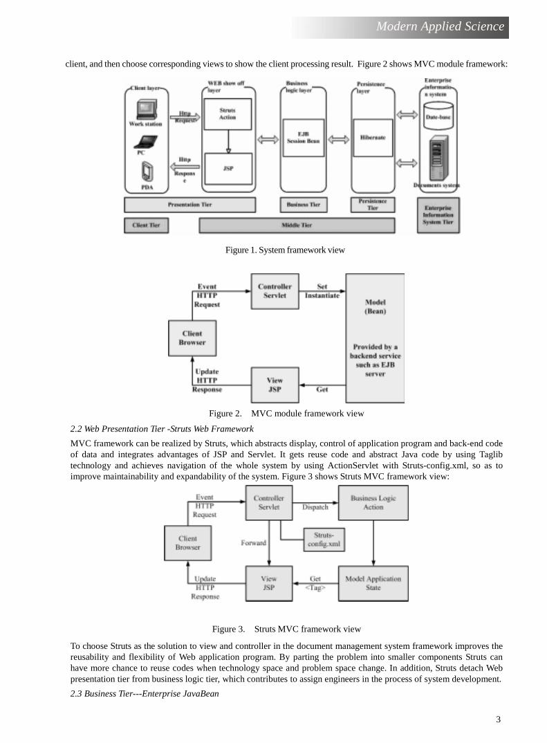
In this project, we choose MVC (Model/View/Controllers) whole framework and Struts Web Framework technology assolution of presentation tier, Enterprise Session Bean technology as solution of business logic tier, Hibernate technologyas solution of persistence tier. See Figure 1.

2.1 MVC Module Framework of Document Management

MVC is a program method and framework which is based on object-oriented design thought. Its core idea is to reduce theinterdependence of all tiers and loose the relation of all modules in order to make best reuse of them. In this MVC framework,application program is divided into three core components: Model, View and Controller. They execute their tasks respec-tively and separate input, processing and output of application program forcibly. To apply MVC framework can detach coredata access function from data presentation and logic control. This detachment will make the whole system form anincompact coupling framework, so that the system design is clear and possesses reusability, expansibility and flexibility.

The document management system framework based on MVC is very flexible. It can connect different modules and viewsto meet clients’ demand with controller. Therefore, the controller can provide forceful means for setting up applicationprogram. Through some reusable modules and views the controller can process the modules according to the demand of

3

Modern Applied Science

client, and then choose corresponding views to show the client processing result. Figure 2 shows MVC module framework:

Figure 1. System framework view

Figure 2. MVC module framework view

2.2 Web Presentation Tier -Struts Web Framework

MVC framework can be realized by Struts, which abstracts display, control of application program and back-end code of data and integrates advantages of JSP and Servlet. It gets reuse code and abstract Java code by using Taglib technology and achieves navigation of the whole system by using ActionServlet with Struts-config.xml, so as to improve maintainability and expandability of the system. Figure 3 shows Struts MVC framework view:

Figure 3. Struts MVC framework view

To choose Struts as the solution to view and controller in the document management system framework improves the reusability and flexibility of Web application program. By parting the problem into smaller components Struts can have more chance to reuse codes when technology space and problem space change. In addition, Struts detach Web presentation tier from business logic tier, which contributes to assign engineers in the process of system development.

2.3 Business Tier---Enterprise JavaBean

4


EJB can meet the demands of enterprise system in versatility, expandability, portability, fast construction and customization.It provides a framework to develop and execute distributed business logic, which simplifies development of expandable andextreme complex application system. In addition, EJB container takes charge of public services, such as JNDI, JTS, safety,resource buffer pool and fault-tolerant processing. This document management, which uses EJB as solution to business tierto achieve module of MVC framework, can meet the demand of enterprise business.

2.4 Persistence Tier--Hibernate

Data persistence is a very important link in the development process of enterprise application program. It means that datain outside storage medium (such as database and flat document system)can be protected for a long time even if applicationserver is broken down.

In J2EE framework, the standard of realizing data persistence is to map from object expressed by object model to relationalmodel data structure by Bean in EJB component model. And in the actual application it appears high consumption, lowperformance, complex configuration and general development efficiency in Entity Bean memory. Hibernate is an excellentlightweight O/R Mapping framework of open source code. It packages JDBC and simplifies program of data persistence. Itmaps from object expressed by object model to relational model database and provides means of inquiring and obtainingdata, which greatly reduces the time to use SQL and JDBC processing data manually. It is convenient to use object-orientedprogramming thought to manipulate database. The application of Hibernate lower the application difficulty in using largeand complex enterprise J2EE framework . In fact, it is so simple and practical that Hibernate is widely applied in the processof enterprise information construction.

2.5 Application Server-JBoss Application Server

JBoss Server is applicable to develop, integrate, deploy and manage large distributed Web application, network applicationand database application. It introduces dynamic function of Java and safety of J2EE into development, integration, deploy-ment and management of large network application. Both webpage cluster and component cluster are critical to expandabilityand usability needed by document management. JBoss Server realizes not only webpage cluster but EJB component cluster.Meanwhile, it needs no support from any special hardware and operation system. The enterprise application system ofdocument management should be developed rapidly. It requires that server components possesses not only good flexibilityand safety, but expandability and strong usability to support key task. JBoss Sever can meet the demand of enterpriseapplication system development of document management. It simplifies the development of portable and extendable appli-cation system and provides rich interoperability for the other application systems.

3 .System Function

Figure 4. Functional configuration of product database management system

3.2 Module of System Function

This system includes five modules: organization structure and access control management, product structure and versionmanagement, design index and part library management, workflow and process management, project management.

3.2.1 Organization structure and access control management

By this module enterprise can control all staff to operate database according to their duties. Its main functions are to set upand maintain enterprise organization structure, carry out access control management of project data in the process ofproduct design, including authorization and verification, and provide the basic support for the operation of the other

5


modules.

3.2.2 Product structure and version management

This module is in charge of setting up and maintaining complete product structure tree model. Its main functions includecreation of product structure tree, dynamic tier view, storage version of parts in design procedure. This system canautomatically get product structure information to set up product structure tree from CAX. Each node of product structuretree contains not only CAD/CAE/CAM/CAPP file but all kinds of files produced in design process. Therefore, it can takeproduct as basic unit to orderly organize the related technology document and management document in terms of the waysof organization structure and forms main model of product information.

3.2.3 Design index and part library management

This module provides support for creating new products by reusing present design to the greatest extent. Its functionsmainly include interface of part data, index based on content but not classification, maintenance system of database,transformation mechanism of technical data obtained from design process.

3.2.4 Workflow and process management

Workflow and process management module is to define, execute, track and monitor all the things and activity in the processof product development and project modification. It consists of definition tool of workflow module, workflow engine whichexecutes workflow, workflow monitor and management tool and so on. It defines workflow module according to businessprocess, instantiates workflow module and submits it to workflow executing. It can track the executing condition of workflowby using workflow monitor and management tool. The workflow management in the system plays emphasis on the manage-ment of data and document life cycle. To generate, audit, publish, change and file data can be realized through workflow. Inaddition, management efficiency and quality will be improved by making best use of auxiliary function in workflow andprocess management (such as triggering, warning , notice mechanism and interface of email and so on).

3.2.5 Project management

The design and manufacture of product is a system project, which involves many aspects of project areas. Project manage-ment module is in charge of dividing data process and workflow task into subtasks and allocates related staff, process andworkflow to product project, so as to reduce the complexity of product object management. This module includes fixedvalue, monitor, audit, feedback and submitting of project. With the help of this module, project supervisor can sendprogress reports to project director, with which director may arrange the whole task easily. To some extent, this documentmanagement system can save tremendous resource.

4. Conclusion

As the above stated, in this paper it programs much more overall function module of document management based onadvanced thought of life cycle management. The successful implementation of this system can effectively improve thequality of enterprise knowledge management and achieve knowledge management of product. With this system the enter-prises can stably develop products and enhance competitive power of enterprise, so as to meet with the challenge ofvariable international market environment. We will continue to perfect and extend its function to meet the demand ofenterprises and go further to strengthen the security of system information.

References

Akitoshi Yoshida. (1997). MOWS: distributed Web and cache server in Java. Computer Networks and ISDN Systems. (9):965-975.Scott M. Baker & Bongki, Moon. (1999). Distributed cooperative Web server. Computer Networks. (3):1215-1229.

(2003). Sun Microsystems. Enterprise JavaBeans Specification. Version 2.1.

Wang ,Tingjin. (2002). .An Investigation on Web-based collaborative product structure management.

Zhong, Shisheng, Zhang, Hongyan and Li, Tao. (2005). Study and application of web based document management in PDM.Journal of Haerbing Industry University. (8):1032-1033.

Zhou, Xin, Cen, Zhiwei and Wang, Xiaoping. (2001). Application in enterprise of web based document management.Computer Application and Software. (3):18-19.


6

Vol. 1, No. 3

September 2007

Study on Combined shell Mechanics Analysis

Xiangzhong Meng

College of Marine, Northwestern Polytechnical University, Xi’an 710072, China

Tel: 86-29-8847-4122 E-mail: [email protected]

Xiuhua Shi & Xiangdang Du

College of Marine, Northwestern Polytechnical University, Xi’an, 710072, China

The research is supported by graduate starting seed foundation of Northwestern Polytechnical University. No. Z200510.

Abstract

The AUV combines mostly in ball shell, cylindrical shell, taper shells and other rotary shells by thread coupling, boltcoupling, wedge coupling and hoop coupling. This paper makes the finite element analysis and research on the mechanics mode of a certain AUV with the analytic method. Based on the basic equation of theory of thin shells, analysed every separated shells, and set up it’s mechanics mathematical model, and analysed the combined shell with the finite element method. At last, the final result validated the mathematical model. The method presented is effective in analysing and dynamical designing of AUV structure.

Keywords: Combined shell, Mathematical model, FEA

During the work progress of AUV, such as torpedo and mine, the shell endures the hydraulic pressure. The research of vibration has important theory value and practical meaning on AUV. The AUV is combines mostly in ball shells,column shells, taper shells and other rotary shells by thread coupling, bolt coupling, wedge coupling and hoop coupling. It is shown in figure 1.

1. The basic theoretical equation of thin shell

A middle surface patch of thin shell and internal forces on the cross section are shown in figure 2. The parameters

1N , 2N , 12N , 1M , 2M , 12M , 1Q , 2Q are the internal forces acted on α plane and β plane, 1k and 2k are the maincurvatures on α direction and β direction, 1R and 2R are the radius of main curvature on the middle surface, and

1 11k R= , 2 21k R= , A and B are the Lame coefficients on α direction and β direction, 1p , 2p , 3p are the component of loads on α direction , β direction and γ direction, u , v and w are the component of displacements on α direction, β direction and γ direction of any point on the middle surface of shell.

The balanceable equations of basic equation in the thin shell theory are:

1 2 12 12 1 1 1

2 1 12 12 2 2 2

12 12 1 2 2

12 12 2 1 1

1 1 2 2 1

( ) ( ) 0

( ) ( ) 0

( ) ( ) 0

( ) ( ) 0

( ) ( )

B ABN N N AN ABk Q ABp

A BAN N N BN ABk Q ABp

B ABM M M AM ABQ

A BAM M M BM ABQ

AB k N k N BQ

α α β β

β β α α

α α β β

β β α α

α

∂ ∂ ∂ ∂− + + + + =∂ ∂ ∂ ∂∂ ∂ ∂ ∂− + + + + =∂ ∂ ∂ ∂∂ ∂ ∂ ∂+ − + − =∂ ∂ ∂ ∂∂ ∂ ∂ ∂+ − + − =∂ ∂ ∂ ∂

∂ ∂− + + +∂ ∂ 2 3

(1.1)

( ) 0AQ ABpβ

+ =

From the geometrical equations (1.2) and the physical equations (1.3) of basic equation in the thin shell theory, we can reason out the elastic equations (1.4).

7


1 1

2 2

12

1 1

1 1(1.2)

( ) ( )

u Av k w

A AB

v Bu k w

B AB

A u B v

B A A B

εα β

εβ α

εβ α

∂ ∂= + +∂ ∂∂ ∂= + +∂ ∂∂ ∂= +∂ ∂

1 1 22

2 2 12

12 21 12

( )1

( ) (1.3)1

2(1 )

EhN

EhN

EhN N

ε μεμ

ε μεμ

εμ

= +−

= +−

= =+

1 21

2 12

12

( )1 1

( )1 1(1.4)

2(1 )( ) ( )

N Nu Av k w

A AB Eh

N Nv Bu k w

B AB Eh

NA u B v

B A A B Eh

μα β

μβ α

μβ α

−∂ ∂+ + =∂ ∂

−∂ ∂+ + =∂ ∂

+∂ ∂+ =∂ ∂

The state of nonmomental theory supposed there are no both flexural moment and torsional moment on the any cross section of the thin shell, that is 1 2 12 21 0M M M M= = = = . Equations (1.1) are simplified (1.5).

1 2 12 12 1

2 1 12 12 2

1 1 2 2 3

( ) ( ) 0

( ) ( ) 0 (1.5)

0

B ABN N N AN ABp

A BAN N N BN ABp

k N k N p

α α β β

β β α α

∂ ∂ ∂ ∂− + + + =∂ ∂ ∂ ∂∂ ∂ ∂ ∂− + + + =∂ ∂ ∂ ∂− − + =

1.1 The Cylindrical Shell

The α -axis point to the generatrix and the β -axis point to the circumference of cylindrical shell, then, 1 0k = ,

2 1k R= and 1A B= = , the Gauss-Codazzi conditions are fulfiled. It is shown in figure 3. The balanceable equationsand elastic equations of cylindrical shell nonmomental theory are:

1 121

2 122

2 3

0

0 (1.6)

0

N Np

N Np

N Rp

α β

β α

∂ ∂+ + =∂ ∂∂ ∂+ + =∂ ∂− + =

1 2

2 1

12

(1.7)

2(1 )

N Nu

EhN Nv w

R Eh

Nu v

Eh

μα

μβ

μβ α

−∂ =∂

−∂ + =∂

+∂ ∂+ =∂ ∂

1.2 The Gyral Shell

The parameter 1C is the curvature center of point M on the gyral shell generatrix. It is shown in figure 4. The curvatures are 1 11k R= ( α direction) and 2 21k R= ( β direction) on the middle surface. At the point M,

1 1ds R dα= , 2 2 sinds R dα β= , 1A R= , 2 sinB R α= .

8


The Gauss-Codazzi conditions 1 2( )A

k A kβ β∂ ∂=∂ ∂

and 2 1( )B

k B kα α∂ ∂=∂ ∂

are fulfiled:

21 1

1

1 sincos

dk BdB dR R

d k d d

α αα α α= = = , then 2

1

( sin )cos

d RR

d

α αα

= . The balanceable equations and elastic equations of gyral

shell nonmomental theory are:

1 121 2 1

1 2 2

12 212 2

1 2 2

1 23

1 2

1 1( ) 0

sin

1 2 10 (1.8)

sin

0

N NctgN N p

R R R

N NctgN p

R R R

N Np

R R

αα α β

αα α β

∂ ∂+ − + + =∂ ∂∂ ∂+ + + =∂ ∂

− − + =

1 2

1 1

2 1

2 1 2

122

2

( )1

( )1 cos 1(1.9)

sin sin

2(1 )1 cossin sin

N Nu w

R R Eh

N Nvu w

R R R Eh

Nu v

R Eh

μα

μαα β α

μαα β α α

−∂ + =∂

−∂ + + =∂

+∂ ∂− =∂ ∂

The ball shell is the special gyral shell, and 1A B= = , 1 2 1k k R= = in the ball shell.

2. The axial symmetrical bending equations of thin shell

2.1 The Axial Symmetrical Bending Equations Of Cylindrical Shell

The internal forces, displacements and strains are axial symmetrical in the cylindrical shell. The internal forces reduceto 1N , 2N , 1M , 2M , 1Q , and the displacements reduce to u , w . The axial symmetrical bending equations of the cylindricalshell are:

43

4 2(2.1)

pd w Ehw

d R D Dα+ =

Dimensionless coordinate is brought in, ξ λα= , where 1

42

( )4

Eh

R Dλ = , then

4 2

34

44 (2.2)

d w Rw p

d Ehξ+ =

The approximate solution of equations (2.2) is made up of the nonmomental theory solution ( *w ) and the edge effectsolution ( 0w ), that is,

* 0 *1 2 3 4( cos sin ) ( cos sin ) (2.3)w w w w e C C e C Cξ ξξ ξ ξ ξ−= + = + + + +

In the equation (2.3), the edge effect solution ( 0w ) is the solution on the effect of the flexural moment ( 0M ) and the lateral shearing force ( 0Q ) that are equally distributed along the boundary at the side of 0α ξ= = ,

0 0 03 42 3

0 00 0

1 42

01 0 1 2

1 0 3 0 2

02 1 2

( ) ( )2 2

( ) ( )2

(2.4)( ) ( )

( ) 2 ( )

,

M Qw f f

D D

Q Mdw dwf f

d d D D

QM M f f

Q Q f M f

EhM M N w

R

ξ ξλ λ

λ ξ ξα ξ λ λ

ξ ξλ

ξ λ ξ

μ

= − −

= = +

= +

= −

= =

Where, 1 2 3 4( ) (cos sin ) , ( ) sin , ( ) (cos sin ) , ( ) cosf e f e f e f eξ ξ ξ ξξ ξ ξ ξ ξ ξ ξ ξ ξ ξ− − − −= + = = − = .

2.2 The Axial Symmetrical Bending Equations Of Gyral Shell

The parameters of the gyral shell, 1 11k R= , 2 21k R= , 1A R= , 2 sinB R α= , and on the condition of axial symmetrical bend, 12 12 2 0N M Q= = = and 2 0p = , the axial symmetrical bending balanceable equations of the gyral shell are:

9


1 21 1

1 1 1

1 21

1 1

1 2 13

1 2 1

10

10 (2.5)

0sin

dN N tgQ tg p

R d R R

dM Mtg Q

R d R

N N dQctgp

R R R d

α αα

αα

αα α

− + + =

+ − =

− − − + =

The approximate solution of equations (2.5) is made up of the general solution of the homogeneous equation and thespecial solution of the unhomogeneous equation. The special solution can be solved from the nonmomental theoryequations, and the general solution , the edge effect solution, can be solved by hybrid method. Then the equations (2.5) simplified to the equations (2.6).

0 01 2

11 1 1

1 21

1 1

0 01 2 1

1 2 1

10

10 (2.6)

0sin

dN N tgQ

R d R R

dM Mtg Q

R d R

N N dQctg

R R R d

αα

αα

αα α

− + =

+ − =

+ + =

The basic functions are supposed,0

0

1

1( )dw

uR d

ωα

= + , 2 1R Qφ = − .

The differential operator is supposed,2

2

1 1 1 2

1[ ] [ ( ) ]

R d d ctg d ctgL

R d R d R d R

α αω ωα α α

= + − .

The basic differential equations that the axial symmetrical bending edge effect of gyral shell are:

1

1

( )

(2.7)( )

LR D

L EhR

μ φω ω

μφ φ ω

− =

+ = −

To ball shell, the curvature radius 1 2R R R= = are constants, and 1RQφ = − , then,

2 22

12

221 1

12

( )(2.8)

( )

d d Rctg ctg Q

d d D

d Q dQctg Q ctg Eh

d d

ω ω α ω α μα α

α α μ ωα α

+ − + =

+ − − = −

The effect of edge effect reduce rapidly with the distance increase to boundary, then the equations (2.8) simplified to theequations (2.9):

2 2

12

21

2

(2.9)

d RQ

d D

d QEh

d

ωα

ωα

=

= −

The basic differential equations that the axial symmetrical bending of ball shell are:

4 21

14 0 (2.10)d Q EhR

Qd Dα

+ =

Dimensionless coordinate is brought in,η ϑα= , where 124( )

4EhR

Dϑ = , then,

441

14 4 0 (2.11)d Q

Qd

ϑα

+ =

The internal forces expressions are:

10


01 3 2

202 4 3

1 2 1

2 1

1 3 2

[ ( ) 2 ( )]

2 ( ) 2 ( )

(2.12)( ) ( )

( ) 2 ( )

N Pf M f ctgR

N P f M fR

M P f MfR

M M

Q Pf M fR

ϑη η α

ϑλ η η

ϑ η η

μϑη η

= +

= −

= − +

=

= − −

Where, 1 2 3 4( ) (cos sin ) , ( ) sin , ( ) (cos sin ) , ( ) cosf e f e f e f eη η η ηη η η η η η η η η η− − − −= + = = − = .

3. The analysisi of torpedo

The shell of torpedo is made up of ball shell, cylindrical shell, taper shells and other rotary shells by thread coupling, bolt coupling, wedge coupling and hoop coupling. All of them are rigid coupling. The radius of ball shell 0.25R = , the length of cylindrical shell 5.50L = , the thickness of shell 0.005h = , the elastic modulus 107.47 10E pa= × , the Poisson’s ratio 0.36μ = , inner pressure 6

3 10p pa= .

It is shown the force analysis of the coupling of the ball shell and the cylindrical shell in figure 5.

From the balanceable equations of ball shell nonmomental theory, and 1 2R R R= = , 1 2N N , obtained the result:

* * 31 2( ) ( )

2

RpN N ;

From the balanceable equations of cylindrical shell nonmomental theory, obtained the result: *2 3( )N Rp , * 3

1( )2

RpN .

Obviously, the circumferential direction internal force is not continuous on the coupling circumference, that

is * *2 2( ) ( )N N≠ , so, there is a direct displacement, and the radial alterations are:

23 (1 )

2B

R pa

Ehδ μ= − ,

23 (1 )

2C

R pa

Eh

μδ = − .

The direct displacement is not continuous, and the difference is2

3

2

R pa

Ehδ = . Thus, there must be 0Q and 0M that are

equally distributed along the circumference, so that the continuousness of the internal force and displacement are

ensured. Based on the theory of Timashenko, the rotations of the ball shell and the cylindrical shell are same along the

circumference, so 0 0M = , and the discontinuousness is avoided enough by 0Q .

The direct displacement of the ball shell brought by 0Q is ' 01 32

Qa

Dδ

λ= − , and the cylindrical shell is ' 0

2 32

Qa

Dδ

λ= .

The difference is ' 03

Qa

Dδ

λ= − ,where

1

42( )

4Eh

R Dλ = ,

3

212(1 )Eh

Dμ

=−

.

According to the displacement continuous condition, ' 0a aδ δ+ = , then,

2 3 3233 3 3 3

0 4

12 2 2 84

R p p p pR DQ D

Eh Eh

λ λλλλ

= = = = .

The parameters are counted, then,

3 10 3

2 2

7.47 10 0.005894

12(1 ) 12(1 0.36 )

EhD

μ× ×= = =

− −,

1 1104 4

2 2

7.47 10 0.005( ) ( ) 364 4 0.25 894

Eh

R Dλ × ×= = =

× ×,

124( ) 9

4EhR

Dϑ = =

When 0ξ = ,then 1 3 4 2( ) ( ) ( ) 1 , ( ) 0f f f fξ ξ ξ ξ= = = = ,

When 0η = ,then 1 3 4 2( ) ( ) ( ) 1 , ( ) 0f f f fη η η η= = = = ,

The results of the cylindrical shell are:

11


5 53 31 2

31 2 2 12

31 3

1.25 10 , 1.875 102 2

( ) 0 , 08

( ) 34728

p R p R EhN N w

Rp

M f M M

pQ f

μ

ξ μλ

ξλ

= = × = + = ×

= = = =

= =

The results of the ball shell are:

5 53 3 31 2 3

31 2 2 1

31 3

1.25 10 , ( ) 1.875 102 2 4

( ) 0 , 08

( ) 34728

p R p R pN N f

p RM f M M

pQ f

ϑ ηλ

η μλϑ

ηλ

= = × = + = ×

= − = = =

= − = −

As a result, the circumferential direction internal force is not continuous on the coupling circumference.

References

P. Smithmaitrie & H.S. Tzou. (2004). Micro-control actions of actuator patches laminated on hemispherical shells. Journal of Sound and Vibration. 277, 157-164.

J.H. Ding & H.S. Tzou. (2004). Micro-electromechanics of sensor patches on free paraboloidal shell structronic systems.Mechanical Systems and Signal Processing. 18. 367-380.

Xu, zhilun. (1982). Elastomechanics. The High Education Press.

Figure 1. AUV shell

M1M12

Q1

N1 N12 N2N21

α β

γ

M21M2

α β

γQ2

(a) (b)Figure 2. Space orthogonal coordinate system

N21

N12

N2

N1

R

XY

Z

α

β

Figure 3. Cylindrical

M

Figure 4. Gyral shell

O

Nα O

β

1C

2C

1R

2R

dα

αr

Figure 5. Force analysis of coupling

0 0M= 0 0M =

0Q

0Q


12

Vol. 1, No. 3

September 2007

Modifying Mg/Al Composite Catalyst for

Preparing Narrow-range Distribution Polyether

Bing Pan, Xiujun Liu, Shuangheng Ma, Bin Wang

Department of Material Science and Chemical Engineering

Tianjin Polytechnic University, Tianjin 300160, China


The research is financed by the science and technology development foundational project of Tianjin higher institute. (Grant number: 20050702).

Abstract

The modifying Mg/Al composite catalyst was prepared by co-precipitation method and it was characterized by FTIRand BET. It was used in the ethoxylation between ethanls and EO, and the narrow-range distribution polyethers which have steady properties were prepared. The product was characterized by FTIR and GC/MS. The molecular weight distribution of the product can arrive to 83.28%.

Keywords: Narrow-range distribution, Ethoxylation, Polyether

1. Introduction

The ethoxylation of aliphatic alcohol depicted in Scheme 1 has been utilized for the commercial production of non-ionic surfactants. Similar types of ethoxylations for other organic compounds having active hydrogens have been also applied in the production of various wetting and emulsifying agents (Daehwan Kima, Chengzhe Huang, & Hongsun Lee, 2003:229).

ROH + n H2C CH2

O

catRO CH2CH2O Hx

Scheme 1. ethoxylation of aliphatic alcohol. R: long-chain alkyl group, n: mole ratio of EO/ROH, x: number of ethoxylene units in product mixture.

It is well known that polyether has the superior properties of nontoxicity, flexibility, hydrophilicity, and biocompatibility.These properties are very useful for a polymer used as a drug delivery system (Shaobing Zhou, Xianmo Deng, & Hua Yang, 2003:3566). In recent years, the synthesis of polyester-polyether type block copolymer has attracted much attention, because they can be used in future medical applications in implantation and wound treatment, and as controlledrelease drug carriers (Suh H, Jeong BM, & Rathi R, 1998:336; Jeong BM, Bae YH, & Lee DS, 1997:860;Choi SW, Choi SY, & Jeong BM, 1999:2305).

A great number of patents have recently been published dealing with catalytic systems promoting narrow-range ethoxylation (NRE), i.e. ethoxylation of fatty alcohols with a narrow distribution of the molecular weights of the ethoxylated oligomers and containing a very low concentration of the residual unreacted alcohol. Products of this type have better properties than those produced with the traditional alkaline catalyst KOH and for low ethylene oxide/substrate molar ratio, can be sulphonated without forming undesired dioxane (M. Di Serio, P. Iengo, & R. Gobetto,1996:240). In the ethoxylations of aliphatic alcohols, homogeneous basic catalysts, such as NaOH, KOH or NaOCH3,are generally used to facilitate EO insertion to the alcohols at relatively low temperature and pressure. In this homogeneous type of alcohol ethoxylation, distributions of oxyethylene units in the ethoxylated product mixture are much broader than the statistical Poisson-type distribution. R. Improta had used Aluminium alkoxide sulphate catalysts to promote ethoxylation of fatty alcohols with a narrow distribution of the molecular weights (R. Improta, M. Di Serio and E. Santacesaria, 1999:170).

Hydrotalcite-type solids have been investigated as one group of catalytic materials for the narrow-range oxyethylation

of aliphatic alcohols and esters (Mckenzite A L, Fishel C T, & Davis R J, 1992:548; Rao K K, Gravelle M, 1998:115).

13


Hydrotalcite-type materials are a class of synthetic mixed metal layered hydroxides, generally described by the formula[M1-x

2+Mx3+ (OH) 2][Ax/m

m- ·nH2O], where x may vary from 0.17 to 0.33 depending on the particular combination of divalent M2+ and trivalent M3+ ions. Am- represents the m-valent anion necessary to compensate the positive charge of brucite-like hydroxide layer and locates between mixed metal hydroxide layers (Daehwan Kima, Chengzhe Huang, & Hongsun Lee, 2003:231).

In this paper, we prepared the modified hydrotalcite-type catalysts and report its catalytic properties in ethanol ethoxylation. Otherwise, we characterized the catalyst and product.

2. Experimental 2.1 Materials

Ethanol, Na2CO3, Mg (NO3)2·6H2O, Al (NO3)3·9H2O and Co (NO3)2·6H2O, were of reagent grade and were purchased from Tianjin Chemistry regent Co. (China). EO of 99.9% was supplied from China Petroleum Chem. Co.

2.2 the preparation of Mg/Al composite catalyst

Hydrotalcit-type material was prepared by co-precipitation method at 60? with water-heating method. Na2CO3

solution in 500 ml beaker was added mixed solution of Mg(NO3)2·6H2O, Al(NO3)3·9H2O and Co(NO3)2·6H2O which with 15:5:1 ratio of Mg/Al/Co components with strong mixing and stirring for 1h; pH 8-9 was maintained during theco-precipitation reaction. The white cake was isolated by filtration of the suspension and washed five times with distilled water. The cake was dried for 12 h in air circulating oven at 100? to give white powder and then heated in the tubular stove at 500? for 5h, at last the catalyst was got.

2.3 ethoxylation

Ethoxylation was performed in membrane reactor. The reactor was equipped with a tubular Al2O3 ceramic membranewhich length is 120mm and diameter is 12mm. The catalyst was 1g which was put in the reactor. Ethanol is 1ml/h which was supplied by a piston pump. EO was supplied to the reactor by opening the needle vavle of the EO storage chamber and its velocity was controlled by a rotameter. The reaction was processed at 110? .

2.4 Product analysis

Liquid product was separated by filtration of crude produce and was analyzed using FTIR and GC/MS.

3. Results and discussion

3.1 Characterization of the catalyst

Adding a third metal ion into the complex was to adjust the pore size of catalysts. There is a three-tier electron out of Co 2 + ions so that its volume is bigger than Mg2 + ions. Co 2 + ions were embedded into hydrotalcite structure to adjust the pore size and lead to the hydrotalcite surface lattice defects. After calcination its surface would form a large number of nano-pores and huge amounts of alkaline center which are helpful to the latter reaction.

Figure1shows power IR patterns of the Mg/Al and Mg/Al/Co composite catalyst. The IR patterns of two samples are almost identical. The position of 885cm-1, 744cm-1 is the absorption proportion of metal-oxygen bond. It shows that the entry of Co 2 + has enter into don’t change the crystalline structure.

The specific surface area of modification Mg/Al composite catalyst is 135.8m2/g. High specific surface area is useful for the touch between reactants and alkaline center of the catalyst surface so that the exthoxylation is accelerated.

3.2 Analysis of polyether

Figure 2 shows the IR curve of the product. From the figure 2 we can see the characteristic absorption band: theposition of 3401cm-1 is hydroxyl; the position of 2925 cm-1, 2858 cm-1, 1458cm-1 are methyl, the stretching vibrationand rocking vibration band of methylene respectively and the position of 1112cm-1 is the C-O-C bond skeleton vibration.

The product has been analyzed by the GC/MS. The results show that the selectivity of object product comes to 83.28% which is high than KOH as the catalyst.

4. Conclusions

The modifying Mg/Al composite catalyst was prepared which is very active for narrow-range ethoxylation of ethanol. The products are narrow-range, high purity and light color which have excellent performance in application. From analysis of the product, the selectivity of object product comes to 83.28%.

References

Choi, SW, Choi, SY, & Jeong, BM. (1999). Thermoreversible gelation of poly(ethylene oxide) biodegradable polyester block copolymers. J Polym Sci A. 37(14), pp. 2305-2317.

14


Daehwan, Kima, Huang, Chengzhe & Hongsun Lee. (2003). Hydrotalcite-type catalysts for narrow-range oxyethylation of 1-dodecanol using ethyleneoxide. Applied catalysis A: General. 249(2), pp. 229-240.

Jeong, BM, Bae, YH, & Lee, DS. (1997). Biodegradable blocks copolymers as injectable druf-delivery system. Nature.338, pp. 860-862.

M. Di Serio, P. Iengo, & R. Gobetto (1996). Ethoxylation of fatty alcohols promoted by an aluminum alkoxide sulphate catalyst. Journal of Molecular Catalysis A: Chemical. 112(2), pp. 235-251.

Mckenzite A L, Fishel C T, & Davis R J. (1992). Investigation of the surface structure and basic properties of calcined hydrotalcites. J Catal. 138(2), pp. 548-560.

R. Improta, M. Di Serio, & E. Santacesaria. (1999). Aluminium alkoxide sulphate catalyst: a computational study. Journal of Molecular Catalysis A: Chemical. 137(1-3), pp. 169-182.

Rao K K, & Gravelle M. (1998). Activation of Mg-A1 hydrotacite catalyst for aldol condensation reaction. J Catal. 173, pp. 115-121.

Suh, H, Jeong, BM, & Rathi, R. (1998). Regulation of smooth muscle cell proliferation using paclitaxel-loaded poly (ethylene oxide)-poly (lactide/glycolide)nanospheres. Biomed J Mater Res. 42(2), pp. 331-338.

Zhou, Shaobing, Deng, Xianmo & Yang, Hua. (2003). Biodegradable poly (e-caprolactone)-poly (ethylene glycol) blocks copolymers: characterization and their use as drug carriers for a controlled delivery system. Biomaterials. 24(3), pp. 3563-3570.

Figure 1. FT-IR adsorption spectra of (1) Mg/Al, (2) Mg/Al/Co

Figure 2. FT-IR spectra of the product

15

Science News

Battling Bitter Coffee: Chemists Identify Roasting as the Main Culprit


Science Daily, August 22, 2007

Science Daily-Bitter taste can ruin a cup of coffee. Now, chemists in Germany and the United States say they have identifiedthe chemicals that appear to be largely responsible for java’s bitterness, a finding that could one day lead to a better tastingbrew. Their study, one of the most detailed chemical analyses of coffee bitterness to date, was presented at the 234thnational meeting of the American Chemical Society.

Research by others over the past few years has identified an estimated 25 to 30 compounds that could contribute to theperceived bitterness of coffee. But the main cause of coffee bitterness has remained largely unexplored until now, theresearchers say.

“Everybody thinks that caffeine is the main bitter compound in coffee, but that’s definitely not the case,” says study leaderThomas Hofmann, Ph.D., a professor of food chemistry and molecular sensory science at the Technical University ofMunich in Germany. Only 15 percent of java’s perceived bitterness is due to caffeine, he estimates, noting that caffeinatedand decaffeinated coffee both have similar bitterness qualities.

“Roasting is the key factor driving bitter taste in coffee beans. So the stronger you roast the coffee, the more harsh it tendsto get,” Hofmann says, adding that prolonged roasting triggers a cascade of chemical reactions that lead to the formationof the most intense bitter compounds.

Using advanced chromatography techniques and a human sensory panel trained to detect coffee bitterness, Hofmann andhis associates found that coffee bitterness is due to two main classes of compounds: chlorogenic acid lactones andphenylindanes, both of which are antioxidants found in roasted coffee beans. The compounds are not present in green (raw)beans, the researchers note.

“We’ve known for some time that the chlorogenic acid lactones are present in coffee, but their role as a source of bitternesswas not known until now,” Hofmann says. Ironically, the lactones as well as the phenylindanes are derived from chloro-genic acid, which is not itself bitter.

Chlorogenic acid lactones, which include about 10 different chemicals in coffee, are the dominant source of bitterness inlight to medium roast brews. Phenylindanes, which are the chemical breakdown products of chlorogenic acid lactones, arefound at higher levels in dark roasted coffee, including espresso. These chemicals exhibit a more lingering, harsh taste thantheir precursors, which helps explain why dark-roasted coffees are generally more bitter, Hofmann says.

The type of brewing method used can also influence the perception of bitterness. Espresso-type coffee, which is madeusing high pressure combined with high temperatures, tends to produce the highest levels of bitter compounds. Whilehome-brewed coffee and standard coffee shop brews are relatively similar in their preparation methods, their perceivedbitterness can vary considerably depending on the roasting degree of the beans, the amount of coffee used, and the varietyof beans used.

Some instant coffees are actually less bitter than regular coffee, Hofmann says. This is because their method of preparation,namely pressure extraction, degrades some of the bitter compounds. In some cases, as much as 30 to 40 percent fewerchlorogenic acid lactones are produced, leading to a reduced perception of bitterness, he says.

“Now that we’ve clarified how the bitter compounds are formed, we’re trying to find ways to reduce them,” Hofmann says.He and his associates are currently exploring ways to specially process the raw beans after harvesting to reduce theirpotential for producing bitterness. They are also experimenting with different bean varieties in an effort to improve taste. Butso far, none of these approaches - details of which are being kept confidential by the researchers - is ready forcommercialization, he notes.

But the researchers are optimistic that a better cup of Joe is just around the corner. Perhaps no one could be happier aboutthe news than Hofmann, who admits that he is an avid coffee-drinker with a passion for the dark-roasted varieties.

Funding for the study was provided by the Technical University of Munich, the University of Muenster, and The Procter

and Gamble Company.


16

Vol. 1, No. 3

September 2007

Smart Container Security: the E-seal with RFID Technology

Jin Zhang & Cuifen Zhang

Institute of Computer Science and Technology, Dalian Maritime University, Dalian 116026,China

E-mail: [email protected]

Abstract

In order to protect cargo from damage, theft, and terrorist threats, business and government turn to wireless sensors and RFID tags, and tradition container is replaced by smart container. In this paper, the basic technical features of RFID systems are described and linked to the practical applications. This paper will also determine how the technologies perform in the real-world operational environments and evaluate the various trade-offs that exist with E-seal design.

Keywords: Smart container, RFID technology, Electronic Container Seal (E-seal)

1. Background

Cargo seals are more common in international trade than for domestic shipments. This reflects the historical and continuing importance of Customs duties and cross-border smuggling. Manual cargo seals have long been part of good security practice. Their principal purpose is to assure carriers, beneficial owners of cargo.

Manual seals vary widely in the degree of protection they offer. Many factors affect protection, including the design, materials, and construction of the locking device, and the design and materials in the hasp, bolt, or cable. The trade abounds with tales of popular manual seal designs that have been copied with cheap materials. There are no international standards for manual seals.

Good seal practices improve the odds but cannot guarantee shipment integrity. Clever miscreants can defeat seals in numerous ways, such as cutting holes in the side or top of a container and then repairing it. However, the effectiveness of seal programs seems more affected by poor practices than by unusually skillful criminals.

2. Smart container

Cargo container with smart systems alters globe network in real time about security beaches. The smart system is open, flexible and modular in design. This will enable users to configure other sensors or automatic identification technologies in combinations applicable to their security or cargo management needs. Other container sensors can include hazardous chemical detection and various physical parameters including temperature, light, vibration, shock, atmospheric pressure and so on.

3. Electronic Container seal (E-seal)

E-seal ensure that ever-increasing cargo loads also have far greater protection. These seals, combining robust mechanical parts with sophisticated sensors, deliver a highly cost-effective solution for the cargo industry. An E-Seal is a radio frequency device that transmits container information as it passes a reader device, and issues alerts and error conditions if the container has been tampered with or damaged. E-Seals serve both commercial and security interests by tracking commercial container shipments from their point of origin, while en route, and to their final destination and point of customs clearance.

3.1E-seal technology

E-seals marry manual seal elements with electronic components to measure seal integrity, store data, and provide communications. Some designs use infrared signals and others use direct contact communications technologies, but radio frequency identification (RFID) is the most common choice. Most e-seal designs automate the essential functions of seal checking and reporting in order to remove human intervention. [a]

RFID has long been touted as the future of logistics for all companies by allowing retailers and suppliers to track goods throughout the supply chain. Global logistics company Schenker is testing the use of radio frequency identification (RFID) technology to track containers used for overseas shipments.

4. RFID Seal

17


RFID is the system technology that recognizes a human or material by radio information communication and writes addi-tional information through the media of a card/tag that is built-in IC chip or resonance material.

44444.....11111SSSSSyyyyysssssttttteeeeemmmmm cccccooooonnnnnfffffiiiiiggggguuuuurrrrraaaaatttttiiiiiooooonnnnnThe purpose of the system is to communicate data between informational medium (that is called “RF tag”, “Transponder”of the shape of the card/tag) and an interrogator (that is called “Reader”, “Interrogator”) by the electric wave.

4.2Features and Classification

Recognizable from a distance; Recognizable through an obstacle; Reading two or more tags simultaneously is possible;Writing additional information is also possible; RF tag is reusable.

There are two main types of RFID tags and seals, passive and active.

Passive seals do not initiate transmissions—they respond when activated by the energy in the signal from a reader.Interrogated by a reader, a passive seal can identify itself by reporting its “license plate” number, analogous to a standardbar code. The tag can also perform processes, such as testing the integrity of a seal. The beauty of a battery-free passiveseal is that it can be a simple, inexpensive, and disposable device. Passive RFID seals can carry batteries for either or bothof two purposes. The first is to aid communication by boosting the strength of the reflective signal back to the reader. Thiscapability need not add much cost. The second purpose is to provide power so functions can be performed out of the rangeof readers.

Active seals can initiate transmissions as well as respond to interrogation. All active tags and seals require on-board power,which generally means a battery.

All active RFID electronic seals on or approaching the market monitor seal integrity on a near-continuous basis, and mostcapture the time of tampering and write it to an on-board log. Some can accept GPS and sensor inputs, and some can providelive “mayday” tampering reports as the events happen, mostly within specially equipped terminals.

Passive vs. Active RFID seals. One may look at the trade-offs between these technologies from theoretical and practicalperspectives. Theoretically, the only difference between passive and active tags and seals is the ability to initiate commu-nications from the tag—distinction that means passive RFID tags could not initiate mayday calls. However, a designercould add on-board power to a passive tag, match other functionality and, setting aside regulatory, safety, and cost issues,increase read range and directional flexibility by increasing power and adding antennas.

4.3Standards and Frequencies

Adoption of RFID in supply chain and security applications is hampered by a lack of standards and by what some call “thefrequency wars.” The two issues are interrelated. Standards for electronic seals address technical protocols, interfaces, andfrequencies. There are three related items.

ISO 10374 is the existing voluntary standard for RFID automatic identification of freight containers. It is a dual frequencypassive read-only standard that includes 850-950 and 2400-2500 MHz. Globally, only two carriers use these tags, oneprimarily on chassis and the other on chassis, ocean containers, and many dray trucks.

ISO 18185 is a Draft International Standard for electronic container seals. It includes passive and active protocols, enablingboth simple low cost and more robust seals. The active protocols have been the focal point for “the frequency wars” interms of freight containers.

ISO 23359 is a New Work Item for read/write RFID for freight containers. Work started on this project in June 2002, and itseems likely to build closely on the draft seal standard.

Frequency choice begins with technical performance but includes political and regulatory issues. In crowded freight-oriented environments such as warehouses and terminals, the most effective frequencies appear to be between 100 and 1000

Figure 1.

18


MHz. Frequencies below 100 MHz lose range rapidly because of inductive coupling or noise from electrical coupling.Frequencies above 1000 MHz, with shorter wavelengths, cannot wrap or diffract around objects such as vehicles andfreight containers-they become more line-of-sight and subject to blind spots.

5. Looking Ahead

Container shipping is a critical component of global trade: about 90% of global trade is transported in cargo containers.Globalization and market deregulation have also led to advances in security devices and instruments and their strategicintegration within the logistics sector. The market for E-seal that may improve both freight transportation security andproductivity is in its early stages. We will become a big winner of market in development through relatively early stages ofuse.

References

Hu, Jianyun, He, Yan & Min, Hao. (2006). Design and Analysis of Analog Front-End of Passive RFID Transponders.Chinese Journal of Semiconductors. Vol.27 No.6 p.999-1005

Jung-Hyun Cho, et. (2005). An analog front-end IP for 13.56MHz RFID interrogators. Proceedings of the 2005 conferenceon Asia South Pacific design automation. p. 1208 – 1211.

Le-Pong Chin & Chia-Lin Wu. (2004). The Role of Electronic Container Seal (E-Seal) with RFID Technology in the Con-tainer Security Initiatives. MEMS, NANO and Smart Systems, 2004. ICMENS 2004. Proceedings. 2004 International Con-ference on Aug. p.116- 120.

(2003). International standard ISO/IEC 14443 -1, -2, -3, International Standardization Organization. April.

Vol. 1, No. 3

September 2007

19


Strong Cconvergence Theorems for Strictly Pseudocontractive

Mappings by Viscosity Approximation Methods

Meijuan Shang

Department of Mathematics, Tianjin Polytechnic University, Tianjin 300160, China

Department of Mathematics, Shijiazhuang University, Shijiazhuang 050035, China


Guoyan Ye


Abstract

In this paper, we introduce a modified Mann iterative process for strictly pseudocontractive mappings and obtain a strong convergence theorem in the framework of Hilbert spaces. Our results improve and extend the recent onesannounced by many others.

Keywords: Strong convergence, Strictly pseudocontractive mappings, Viscosity approximation methods

1. Introduction and Preliminaries

Let H be a real Hilbert space, C a subset of H . Recall that A mapping :T C C→ is said to be a strict pseudo-contraction (Browder & Petryshn, 1967, 197-228) if there exists a constant 0 1k≤ < such that

2 2 2( ) ( ) ,Tx Ty x y k I T x I T y− ≤ − + − − − For all ,x y C∈ . (1.1)

(If (1.1) holds, we also say that T is a k -strict pseudocontraction.) Strict pseudocontractions in Hilbert spaces were

introduced by Browder and Petryshyn (1967, 197-228), which are extension of extensions of nonexpansive mappings

which satisfy the inequality (1.1) with 0k = . That is, :T C C→ is nonexpansive if Tx Ty x y− ≤ − , for all ,x y C∈ .

Mann's iteration process (Mann, 1953, 506-510) which is defined as

n+1 n n n nx = x + (1- )Tx , n 0α α ≥ , (1.2)

where the initial guess 0x is taken in C arbitrarily and the sequence{ } 0n nα ∞

=is in the interval [0,1] is often used to

approximate a fixed point of a nonexpansive mapping. However, Mann's iteration process has no strong convergence

for nonexpansive maps even in Hilbert spaces (Genel & Lindenstrass, 1975, 81-86). If T is a nonexpansive mapping

with a fixed point and if the control sequence { } 0n nα ∞

=is chosen so that

0

(1 )n nn

α α∞

=

− = ∞ , then the

sequence{ }nx generated by Mann's algorithm (1.2) converges weakly to a fixed point ofT . This is also valid in a

uniformly convex Banach space with a Frechet differentiable norm (Reich, 1979, 274-276). Attempts to modify the

Mann iteration method (1.2) so that strong convergence is guaranteed have recently been made. Recently, Kim and Xu

(2005, 51-60) modified Mann iterative process to get a strong convergence theorem for nonexpansive mappings. In

(Moudafi, 2000, 46-55), Moudafi proposed a viscosity approximation method of selecting a particular fixed point of a

given nonexpansive mapping in Hilbert spaces.

Recently Xu (2004, 279-291)

Studied the viscosity approximation methods proposed by Moudafi (2000, 46-55) for nonexpansive mappings in a uniformly smooth Banach space. More precisely, he proved following theorems.

Theorem 1.1 (Xu, 2004, 279-291). Let E be a Hilbert space, C a closed convex subset of E and :T C C→ a

nonexpansive mapping with ( )F T φ≠ and Cf ∈Π . Then the sequence{ }nx defined by ( ) (1 ) ,t t tx tf x t Tx= + −

20


(0,1)t∈ converges strongly to a point in ( )F T . If we define : ( )CQ F TΠ → by0

( ) lim tt

Q f x→

= the ( )Q f solves the variational inequality ( ) ( ), ( ) 0I f Q f Q f x− − ≤ , Cf ∈Π , ( )x F T∈ .

In this paper, we try to modified Mann iterative scheme (1.2) for strictly pseudocontractive mappings to have strong

convergence theorem by using viscosity approximation methods in the framework of Hilbert spaces. More precisely, we

introduce the composite iteration process as follows:

1

(1 ) ,

( ) (1 ) .n n n n n

n n n n n

y x Tx

x f x y

β βα α+

= − += + −

(1.3)

We prove, under certain appropriate assumptions on the sequences { }nα and { }nβ that { }nx defined by (1.3)

converges to some fixed point of T , which solves some variational inequality.

It is our purpose in this paper is to introduce this composite iteration scheme for approximating some fixed point of strictly pseudocontractive mappings by using viscosity methods in the framework of Hilbert spaces. We establish the strong convergence of the sequence{ }nx defined by (1.3). Our results improve and extend the ones announced by Kim and Xu (2005, 51-60), Xu (2004, 279-291) and some others.

We need the following lemmas for the proof of our main results.

Lemma 1.1 (Xu, 2002, 240-256). Let { }nα be a sequence of nonnegative real numbers satisfying the

property 1 (1 )n n n n nα γ α γ σ+ ≤ − + , 0n ≥ , where{ } 0(0,1)n n

γ ∞

=⊂ and{ } 0n n

σ ∞

=such that

(i) lim 0nn

γ→∞

= and0

nn

γ∞

=

= ∞ ,

(ii) limsup 0nn

σ→∞

≤ or0

n nn

γ σ∞

=

< ∞ .

Then lim 0nn

α→∞

= .

2. Main Results

Theorem 2.1 Let C be a closed convex subset of a Hilbert space E and let :T C C→ be a strictly pseudocontractive

mapping with a fixed point in C . The initial guess 0x C∈ is chosen arbitrarily and given sequences{ } 0n nα ∞

=and

{ } 0n nβ ∞

=satisfying the following conditions:

(i) lim 0nn

α→∞

= and0

nn

α∞

=

= ∞ ;

(ii) 0 na β γ< ≤ < for some (0, ]a γ∈ and { }min 1,2kγ = ;

(iii) 10

n nn

α α∞

+=

− < ∞ and 10

n nn

β β∞

+=

− < ∞ .

Let { } 0n nx

∞

=be the composite process defined by (1.3). Then { } 0n n

x∞

=converges strongly to some fixed point

( )p F T∈ which solves the variational inequality

( ) ( ), ( ) 0I f Q f Q f p− − ≤ , Cf ∈Π , ( )p F T∈ . (2.1)

Proof. First we observe that{ } 0n nx

∞

= is bounded. Indeed, taking a fixed point p of ( )F T and using (1.1), we have

21


that2

ny p− =2

( ) ( )n n n nx p Tx xβ− + − 2 222 ,n n n n n n n nx p x Tx x p x Txβ β= − − − − + −

2 2(2 )n n n n nx p k x Txβ β≤ − − − − 2

nx p≤ − . (2.2)

It follows from (2.2) that

1 ( ) (1 )n n n n nx p f x p y pα α+ − ≤ − + − − 1max ( ) ,

1 nf p p x pα

≤ − −−

.

Now, an induction yields

nx p− 0

1max ( ) ,

1f p p x p

α≤ − −

−, 0n ≥ , (2.3)

Which implies that { }nx is bounded, so is{ }ny .

Since condition (i), we obtain 1 ( ) 0n n n n nx y f x yα+ − = − → , as n →∞ . (2.4)

Next, we claim that 1 0n nx x+ − → , as n →∞ . (2.5)

On the other hand, we have

1 1 1 1 1 1(1 ) ( )n n n n n n n n n n n nx x y y y f x x xα α α αα+ − − − − −− ≤ − − + − − + − . (2.6)

Next, we define (1 )n n nA T Iβ β= + − . We have nA is nonexpansive for all n . Indeed, It follows from conditions (ii) and

(iii) that

2

n nA x A y− 2[ ( )]nx y x y Tx Tyβ= − − − − −

2 2(2 )n nx y k x Tx y Tyβ β≤ − − − − − + 2

x y≤ − .

Next, we show ( ) ( )nF T F A= . Notice that ( ) ( )np F A p Tp p F T∈ ⇔ = ⇔ ∈ . That is, ( ) ( )nF T F A= .

Observing n n ny A x= and 1 1 1n n ny A x− − −= , we obtain

1n ny y −− 1 1 1 1n n n n n n n nA x A x A x A x− − − −≤ − + − 1 1 1n n n nx x M β β− −≤ − + − . (2.7)

where 1 0M ≥ is a constant such that { }10

sup n nn

M x Tx≥

= + .

Substitute (2.7) into (2.6) yields that

1n nx x+ − 1 2 1 1[1 (1 ) ] ( )n n n n n n nx x Mα α α α β β− − −≤ − − − + − + − , (2.8)

where 2 0M ≥ is a constant such that { }2 1 1 1max ( ) ,n nM y f x M− −≥ − , for all n . By assumptions (i)-(iii) and Lemma

1.1, we obtain (2.5) holds. Observe that

n n n n nTx x y xβ − = − . (2.9)

On the other hand, we have 1 1n n n n n ny x y x x x+ +− ≤ − + − . (2.10)

It follows from (2.4) and (2.5) that lim 0n nny x

→∞− = , (2.11)

which combines with the condition (ii) and (2.9) yields that lim 0n nnTx x

→∞− = . (2.12)

22


Next, we claim that limsup ( ) , 0nn

f q q x q→∞

− − ≤ , (2.13)

where0

( ) lim tt

q Q f s x→

= = − with tx being the fixed point of the contraction ( ) (1 )x tf x t Ax+ − ,

where (1 )A a I aT= − + is a nonexpansive mapping such that ( ) ( )F T F A= . From tx solves the fixed point

equation ( ) (1 )t t tx tf x t Ax= + − , we have (1 )( ) [ ( ) ]t n t n t nx x t Ax x t f x x− = − − + − .

It follows from Lemma 1.2 that

2 2 22(1 2 ) ( ) 2 ( ) , 2t n t n n t t t n t nx x t t x x f t t f x x x x t x x− ≤ − + − + + − − + − , (2.14)

where ( ) (2 ) 0n t n n n n nf t x x x Ax x Ax= − + − − → , as n →∞ . (2.15)

It follows that2 1

( ), ( )2 2t t t n t n n

tx f x x x x x f t

t− − ≤ − + . (2.16)

Let n →∞ in (2.16) and note (2.15) yields limsupn→∞

( ),2t t t n

tx f x x x M− − ≤ . (2.17)

where 0M ≥ is a constant such that2

t nM x x≥ − for all (0,1)t∈ and 1n ≥ . Taking 0t → , from (2.17), we

have0

limsupt→

limsupn→∞

( ), 0t t t nx f x x x− − ≤ . Since H is a Hilbert space the order of0

limsupt→

and lim supn→∞

is

exchangeable, and hence (2.13) holds.

Finally, we show that nx q→ strongly and this concludes the proof. Indeed, we have

2 2

1 (1 )( ) [ ( ) ]n n n n nx q y q f x qα α+ − = − − + −

221(1 ) 2 ( ) ,n n n n ny q f x q x qα α +≤ − − + − −

≤ 221 1(1 ) 2 ( ) ( ), 2 ( ) ,n n n n n n nx q f x f q x q f q q x qα α α+ +− − + − − + − −

2 2 221 1(1 ) ( ) 2 ( ) ,n n n n n n nx q x q x q f q q x qα αα α+ +≤ − − + − + − + − − .

Therefore, we obtain

2

1nx q+ −2

2

1

1 (2 ) 2( ) ,

1 1n n n

n nn n

x q f q q x qα α α ααα αα +

− − +≤ − + − −

− −

2

1

2(1 ) 2(1 ) 1[1 ] [ ( ) , ]

1 1 2(1 ) 1n n n

n nn n

Mx q f q q x q

α α α α ααα αα α α +− −

≤ − − + + − −− − − −

.

Now we apply Lemma 1.1 to see that 0nx q− → . This completes the proof.

References

Browder, F. E. & Petryshn, W. V. (1967). Construction of fixed points of nonlinear mappings in Hilbert spaces. J. Math.Anal. Appl.. 20:197-228.

Genel, A. & Lindenstrass, J. (1975). An example concerning fixed points. Israel J. Math., 22: 81-86.

Kim, T.H. & Xu, H.K. (2005). Strong convergence of modified Mann iterations. Nonlinear Anal. 61: 51-60.

Mann, W.R. (1953). Mean value methods in iteration. Proc. Amer. Math. Soc. 4: 506-510.

Moudafi, A. (2000). Viscosity approximation methods for fixed points problems. J. Math. Anal Appl. 241: 46-55.

Reich, S. (1979). Weak convergence theorems for nonexpansive mappings in Banach spaces. J. Math. Anal. Appl. 67:274-276.

Xu, H.K. (2002). Iterative algorithms for nonlinear operators. J. London Math. Soc. 66: 240-256.

Xu, H.K. (2004). Viscosity approximation methods for nonexpansive mappings. J. Math. Anal. Appl. 298: 279-291.

23

Science News

Sewage Tells Tales about Community-wide Drug Abuse



Public health officials may soon be able to flush out more accurate estimates on illegal drug use in communities across thecountry thanks to screening test described here today at the 234th national meeting of the American Chemical Society. Thetest doesn’t screen people, it seeks out evidence of illicit drug abuse in drug residues and metabolites excreted in urine andflushed toward municipal sewage treatment plants.

The approach could provide a fast, reliable and inexpensive way to track trends in drug use at the local, regional or statelevels while preserving the anonymity of individuals, says lead researcher Jennifer Field, Ph.D., an environmental chemistat Oregon State University who works with colleagues at Oregon State University and at the University of Washington.

Past estimates of illicit drug abuse in a community were based largely on surveys in which children and adults were askedabout their use of illegal drugs. Researchers knew that some were untruthful, with individuals reluctant to admit breaking thelaw.

Preliminary tests conducted in 10 U.S. cities show the method can simultaneously quantify methamphetamine and metabo-lites of cocaine and marijuana and legal drugs such as methadone, oxycodone, and ephedrine, according to Aurea Chiaia, agraduate student who is working to refine the process and described details at the ACS meeting.

“Because our method can provide data in real time, we anticipate it might be used to help law officials undertaking surveil-lance to make intervention or prevention decisions or to decide where to allocate resources,” Chiaia says.

Recently, scientists have sought ways to gauge illegal drug use by measuring the levels of drugs and their by-productsfound in rivers and wastewater. Last year, Italian scientists found ways to detect metabolites for cocaine in the Po River,giving law enforcement officials more accurate estimates on cocaine use in the area. The U.S. Office of National DrugControl Policy has obtained samples from a dozen different waterways in an effort to assess illegal drug use, as well.

Field says the new screening method under development in her lab improves upon the utility of the laboratory toolscurrently used to identify traces and metabolites of drugs in such studies. Tandem mass spectrometry, for example, is alaboratory method routinely used to identify the unique by-products of various drugs by determining their molecularweight. The problem is, the method frequently requires a time-consuming off-line process to concentrate the samples.

Field and her colleagues have eliminated that step. “By streamlining this process, we can cut back on the use of solventsand bring about a savings in time, therefore saving money,” Field says.

Her lab is now refining the technique to verify its accuracy for extremely low concentrations, on the order of a fewnanograms (billionths of a gram) per liter. Calculations of drug use based solely on byproducts found in water supplies,especially at low levels, can be subject to error, Field says. To address this issue, her lab is working to identify commonindicators, or biomarkers, such as caffeine or nicotine that can be used to sharpen their calculations.

“A lot of things contribute to the flow in wastewater, including agricultural and industrial processes,” Field says. “Bylinking our illicit drug measurements to biomarkers related to measurable human activities, we could compensate for differ-ences in flows that aren’t related to human excretion.”

The method would eliminate the need to rely on surveys, medical records and crime reports to assess the scope of acommunity’s drug abuse problem, she says, and allow drug enforcement officials to monitor drug use through time andacross geographic regions.

“If you’re looking for trends over time or space, this will be a suitable methodology,” she says. “By using rapid screeningmethods on a regular basis, we could follow regional (spatial) trends over time in drug use,” she says.

Collaborating with Field and Chiaia are Daniel Sudakin, Ph.D., associate professor of environmental and molecular toxicol-ogy at Oregon State University and Caleb Banta-Green, M.S., a research scientist at the University of Washington’sAlcohol and Drug Abuse Institute.


24

Vol. 1, No. 3

September 2007

A General Projection Method for the System of Relaxed

Cocoercive Variational Inequalities in Hilbert Spaces

Changqun Wu

School of Business and Administration, Henan University, Kaifeng 475001, China

Meijuan Shang


Xiaolong Qin

Department of Mathematics, Tianjin Polytechnic University, Tianjin 300160, China

The research is financed by Henan University .No. 06YBZR034.

Abstract

In this paper, we consider a new algorithm for a generalized system for relaxed cocoercive nonlinear inequalities inHilbert spaces by the convergence of projection methods. Our results extend and improve the recent ones announced by many others.

Keywords: Relaxed cocoercive nonlinear variational inequality, Projection method, Relaxed cocoercive mapping

1. Introduction and preliminaries

Variational inequalities introduced by Stampacchia in the early sixties have had a great impact and influence in the development of almost all branches of pure and applied sciences and have witnessed an explosive growth in theoretical advances, algorithmic development, see [1-6] and references therein.

Let H be a real Hilbert space, whose inner product and norm are denoted by ⋅⋅, and • respectively. Let C be a closed convex subset of H and let HCA →: be a nonlinear mapping. Let CP be the projection of H onto the convex subset C . The classical variational inequality which denoted by ),( ACVI is to find Cu ∈ such that

)1.1(.,0, CvuvAu ∈∀≥−

Recall that A is said to be relaxed ),( vu -cocoercive if there exist two constants 0, >vu such that

)2.1(.,,)(,22

CyxAyAxvAyAxuyxAyAx ∈∀−+−−≥−−

Consider a system (SNVID) of nonlinear variational inequality problems as follows:

Find Czyx ∈*** ,, such that

)3.1(,0,,0,),,( ******1 >∈∀≥−−+ sCxxxyxzyxsT

)4.1(,0,,0,),,( ******2 >∈∀≥−−+ tCxyxzyzyxtT

)5.1(,0,,0,),,( ******1 >∈∀≥−−+ rCxzxxzzyxrT

One can easily see the SNVID problems (1.3), (1.4) and (1.5) are equivalent to the following projection formulas:

,0)],,,([ ***1

** >−= sxzysTyPx C

,0)],,,([ ***2

** >−= tyxztTzPy C

,0)],,,([ ***3

** >−= rzyxrTxPz C

respectively, where CP is the projection of H onto C .

25


2. Algorithms

In this section, we consider an introduction of the general three-step models for the projection methods and its special form can be applied to the convergence analysis for the projection

methods in the context of the approximation solvability of the SNVID problems (1.3)-(1.5).

Algorithm 2.1. For any ,, 00 Cyx ∈ , compute the sequences }{ nx , }{ ny and }{ nz by the iterative processes:

)],,,([ 11311 nnnnCn zyxrTxPz ++++ −=

)1.2()],,,([ 11211 nnnnCn yxztTzPy ++++ −=

)],,,([)1( 11311 nnnnCnnnn zyxrTxPxx ++++ −+−= αα

where }{ nα is a sequence in [0,1] for all 0nn ≥ .

In order to prove our main results, we need the following lemmas and definitions.

Lemma 2.1. Assume that }{ na is a sequence of nonnegative real numbers such that

,,)1( 01 nncbaa nnnnn ≥∀++−≤+ λ

where 0n is some nonnegative integer, }{ nλ is a sequence in (0,1) with )(,1 nnn n ob λλ =∞=∞= and ∞<∞

=0n nc , then0lim =

∞→ nn

a .

Definition 2.1. A mapping HCCCT →××: is said to be relaxed ),( vu -cocoercive if there exist constants 0, >vusuch that, for all ,', Cxx ∈

CzzyyxxvzyxTzyxTuxxzyxTzyxT ∈∀−+−−≥−− ',,',,')',','(),,()('),',','(),,(22

.

Definition 2.2. A mapping HCCCT →××: is said to be μ -Lipschitz continuous in the first variable if there exists a constant 0>μ such that, for all ,', Cxx ∈

CzzyyxxzyxTzyxT ∈∀−≤− ',,',,')',','(),,( μ

3. Main results

Theorem3.1. Let C be a closed convex subset of a real Hilbert space H . Let HCCCT →××:1 be a relaxed),( 11 vu -cocoerceive and 1μ -Lipschitz continuous mapping in the first variable, HCCCT →××:2 be a relaxed ),( 22 vu -cocoerceive and 2μ -Lipschitz continuous mapping in the first variable, HCCCT →××:3 be a relaxed ),( 33 vu -cocoerceive and 3μ -Lipschitz continuous mapping in the first variable. Suppose that Czyx ∈*** ,, are

solutions of the SNVID problems (1.3)-(1.5) and }{},{},{ nnn zyx are the sequences generated by Algorithm 2.1. If }{ nαis a sequence in [0,1] satisfying the following conditions:

;)( 0 ∞=∞=n ni α

};,,min{,,0)( 23

2333

22

2222

21

2111 )(2)(2)(2

μ

μ

μ

μ

μ

μ uvuvuvrtsii −−−<<

};,,)( 2

333

2

222

2

111 μμμ uvuvuviii −−−

then the sequences }{},{ nn yx and }{ nz converges strongly to **, yx and *z , respectively.

Proof. Since ),,( *** zyx is the solution to the SNVID problems (1.3)-(1.5), we have

,0)],,,([ ***1

** >−= sxzysTyPx C

,0)],,,([ ***2

** >−= tyxztTzPy C

,0)],,,([ ***3

** >−= rzyxrTxPz C

Observing (2.1), we obtain

]),,([)1( *

1

*

1 xxzysTyPxxx nnnnCnnnn −−+−=−+ αα )1.3(.)],,(),,([)1( ***

11

** xzyTxzyTsyyxx nnnnnnn −−−+−−≤ αα

By the assumption that 1T is relaxed ),( 11 vu -cocoercive and 1μ -Lipschitz continuous in the first variable, we obtain 2***

11* )],,(),,([ xzyTxzyTsyy nnnn −−−

2***

11

2***

11

** ),,(),,(),,(),,(,2 xzyTxzyTsxzyTxzyTyysyy nnnnnnnn −+−−−−=

)2.3(222*2

1

2*2

122*

1

2*2

11* yyyysyysvyysuyy nnnnn −=−+−−−+−≤ θμμ

Where 2

1

2

1

2

11

2

1 221 μμθ ssvsu +−+= .From the conditions (ii) and (iii), we know 11 <θ .

Substitute (3.2) into (3.1) yields that

)3.3()1( *

1

**

1 yyxxxx nnnnn −+−−≤−+ θαα

Now, we estimate

)4.3(],,(),,([)],,([ ***

2112

*

1

*

1121

*

1 yxzTyxzTtzzyyxztTzPyy nnnnnnnnCn −−−≤−−=− +++++++

26


By the assumption that 2T is relaxed ),( 22 vu -cocoercive and 2μ -Lipschitz continuous in the first variable, we obtain2***

2112*

1 )],,(),,([ yxzTyxzTtzz nnnn −−− +++2***

212

2***

2112

*

1

2*

1 ),,(),,(),,(),,(,2 yxzTyxzTtyxzTyxzTzztzz nnnnnnnn −+−−−−= +++++

)5.3(222*

1

2

2

2*

1

2

2

22*

12

2*

1

2

22

2*

1 zzzztzztvzztuzz nnnnn −=−+−−−+−≤ +++++ θμμ

where 2

22

2

2

22

2

2 221 μμθ ttvtu +−+= . From the conditions (ii) and (iii), we know 12 <θ . Substituting (3.5) into (3.4) yields that *

12

*

1 zzyy nn −≤− ++ θ , which implies that )6.3(*

2

* zzyy nn −≤− θ

Similarly, Substituting (3.6) into (3.3), we have

)7.3()1( *21

**1 zzxxxx nnnnn −+−−≤−+ θθαα

Next, we show that

)8.3(],,(),,([)],,([ ***

3113

*

1

*

1131

*

1 zyxTzyxTrxxzzyxrTxPzz nnnnnnnnCn −−−≤−−=− +++++++

By the assumption that 3T is relaxed ),( 33 vu -cocoercive and 3μ -Lipschitz continuous in the first variable, we obtain 2***

3113

*

1 )],,(),,([ zyxTzyxTrxx nnnn −−− +++2***

3113

2***

2113

*

1

2*

1 ),,(),,(),,(),,(,2 zyxTzyxTrzyxTzyxTxxrxx nnnnnnnn −+−−−−= ++++++

)9.3(222*

1

2

3

2*1

2

322*

13

2*1

2

33

2*1 xxxxrxxrvxxruxx nnnnn −=−+−−−+−≤ +++++ θμμ

where 2

3

2

3

2

33

2

3 221 μμθ rrvru +−+= .From the conditions (ii) and (iii), we know 13 <θ . Substituting (3.9) into (3.8), we obtain *

13

*

1 xxzz nn −≤− ++ θ , which implies )10.3(*

3

* xxzz nn −≤− θ

Similarly, substituting (3.10) into (3.7) yields that

)11.3()]1(1[)1( *

321

*

321

**

1 xxxxxxxx nnnnnnn −−−≤−+−−≤−+ θθθαθθθαα

Noticing that ∞=−∞=0 321 )1(n n θθθα and Applying Lemma 2.1 into (3.11), we can get

the desired conclusion easily. This completes the proof.

References

G. Stampacchia. (1964). Formes bilineaires coercivites surles ensembles convexes. Comptes rendus de I'Academie des Sciences. Paris 258. 4413-4416.

R.U. Verma. (2002). Generalized Partial Relaxed Monotonicity and Nonlinear Variational Inequalities. Int. J. Appl.Math. 9, 355-363.

R.U. Verma. (2004). Generalized System for Relaxed Cocoercive Variational Inequalities and Projection Methods. J. Optim. Theory Appl. 121, 203-210.

R.U. Verma. (2004).Generalized system for relaxed cocoercive variational inequalities and its projection methods. J. Optim. Theory Appl. 121, 203-210.

R.U. Verma. (2007). A -monotone nonlinear relaxed cocoercive variational inclusions. Central European J. Math. 5 (2)386-396.

S.S. Chang, H.W. Joseph Lee & C.K. Chan, (2007). Generalized system for relaxed cocoercive variational inequalitiesin Hilbert spaces. Appl. Math. Lett. 20, 329-334.

Vol. 1, No. 3

September 2007

27


Research on the Method of Modular

Design Based on Product Overall Lifecycle

Jiangtao Li & Minghua Shi

School of Mechanical and Electronic Engineering, Tianjin Polytechnic University, Tianjin 300160, China


Na Sun

Electronic and Communication Engineering Department, North China Electric Power University

Baoding 071003, China

Abstract

All stages in product total lifecycle are a correlative whole which contains the whole closed loop process including acquisition of users’ requirements, acquisition of custom-built product and after service. The traditional modular design takes the modular and function analysis as its main characteristics. This article puts forward the method of modular design based on the product overall lifecycle which is the modular design based on the function partition of the modulesto fulfill the demands of product development. This method is validated and analyzed through the example of the doubling machine in the article.

Keywords: Overall lifecycle, Modular design, Modular optimization

1. Introduction

The modular design takes the module-oriented and function analysis as its main characteristics, and can quickly createproduct series through the selection and combination of the modules. The module partition is one important part of modular design. Its result would directly influence the performance and appearance of the modular products and generaldegree and cost of the modules. In recent years, many foreign and domestic scholars have done much researches in the field of modular technique one after the other. Jianghui and her colleagues of Tianjin University put forward the method which established the full modular matrix to design the modules from the view of the whole, and they also brought forward the method which used the correlation degrees among computational sub-functions to partition the modules(Jiang, 1998, pp.7-9). Du Taojun and his colleagues of Beijing institute of technology put forward the partition method of function modules and structure modules and introduced the relative evaluation method (Du, 2003, pp.50-53). Kusiak and his colleagues applied the heuristic modular recognition-graphic approach and put forward three modular structure forms (Kusiak, 1996, pp.523-528). The above methods of module partition all start from the product function. Though it can resolve the modular structures of one sort or several sorts product, but it rarely relates to the problems of modular assemblage, servicing and recycle and can not fulfill the demands of the whole lifecycle. This article puts forward the method of module partition based on the overall lifecycle, which can optimize the modules for the product overall lifecycle on the basis of function partition and fulfill the demand of product development.

2. Introduction of modular design based on product overall lifecycle

2.1 Concept of modular design

The modular design is the design method which partitions and designs a series of function modules and constitutes different products through the selection and combination of modules on the basis of function analysis to the products with different functions or the products with same functions but different performances and specifications in certain range to fulfill the different demands of the market (Jia, 1993).

2.2 Basic concept of product overall lifecycle design

The product overall lifecycle includes the gestation stage (including the formation of the demands of product market,

product layout and design), the production stage (including material selection, making equipment, product making and

assemblage), the storage and distribution stage (including storage, packaging, transport, distribution, installation and

debugging), the service stage (including product running, examining and repairing), the recycle stage (including

scraping, components reoccupied, regeneration of scrap, recycle of raw and processed materials, disposal of scrap etc.)

28


a

2

TTspm

3

Tt

t

t

3

Wdbsu

3

Goaf

TtIt

3

W

29


Where, ija represents the interaction value of weighted average between the ith and the jth component, and iaaa jijij =≤≤ ,100 .

From the upper triangular matrix of the symmetrical matrix A, we can get the matrix 'A ,

=

nn

ij

n

n

n

a

a

aa

aaa

aaaa

A

...

...0

...

...

...

334

22322

1131211

' .

Then, set down the interaction thresholdλ and cut it, partition the component which threshold is bigger than or equals toλ into one module. The concrete method can be described that: to the ith line, partition all components which interaction value aij fulfills the condition of )1( njaij ≤≤≥ λ into the same module, at the same time, these

components would not participate in the partition of the follow lines, in the same way, until to the nth line, when the partitions are completed, we can get the requested module partition project.

4. Optimization of modular design based on product overall lifecycle

As viewed from the product lifecycle, we must consider the design, manufacturing, assemblage, usage, maintenanceand recycle in the process of module partition. Therefore, on the premise of ensuring the function, we need further optimize the modules according to this partition method.

From the module partition above, we can obtain the module M1, M2, M3… Mn. Now on the basis of that, we partition these modules based on the product overall lifecycle. First we should confirm the factors influencing the interaction among components. The factors in different stages are not independent, and the interventions exist in each other. When analyzing the interaction relation of one certain component to other components, we should synthetically consider the factors in various stages which influence the interactions among components, and deal with the interactive factors through the quantitative ways to satisfy this demand, as Table 1 shows.

4.1 Establishing the interaction matrix taking the module as the unit

When optimizing the modules of the product, we can distribute corresponding weighted factors to the module according to different objects in the product overall lifecycle, [ ]nwwwwW '...'''' 321= under the condition

of 0',1'1

≥==

i

n

i

i ww . Aiming at the hth lifecycle object, according to the interactive relation in Table 1, we set down the

comparison matrix Th (h = 1, 2, 3…n) taking the module as the unit,

=

.....................

...),(),(...),(),(

...),(),(...),(),(

.....................

...),(),(...),(),(

...),(),(...),(),(

......

222221221222112222

222121211221112121

221221121212111212

221121111211111111

22211211

CCTCCTCCTCCTC

CCTCCTCCTCCTC

CCTCCTCCTCCTC

CCTCCTCCTCCTC

CCCC

T

hhhh

hhhh

hhhh

hhhh

h

.

Where, n represents that there are n lifecycle objects, Cij represents the jth component in the ith module, Th(Cij,Cmn) is the interaction value of the hth lifecycle object between component Cij and component Cmn. From the weighted sum of N comparison matrixes, we can get the interaction matrix T among components based on product overall lifecycle.

[ ][ ] ==•= Tnnh wwwwTTTTWTT '...'''...' 321321

),(...),(),(...),(),(

...),(...............

),(...),(),(...),(),(

),(...),(),(...),(),(

.....................

),(...),(),(),(),(

),(...),(),(...),(),(

2111211

22212212212221122

21212112112211121

12211211212121112

11211111112111111

nnnnnnnnnnnnn

mnij

nnn

nnn

nnn

nnn

MMTMMTMMTMMTMMT

MMT

MMTMMTMMTMMTMMT

MMTMMTMMTMMTMMT

MMTMMTMMTMMTMMT

MMTMMTMMTMMTMMT

.

30


Where, T(Mij, Mmn) represents the interaction value of weighted average between the jth component in the ith module and the mth component in the nth module.

4.2 Modular optimization based on product overall lifecycle

According to the interaction matrix T, the quantitative optimization function of the module can be described as the follows:

fJMMTUIM

f

IfIJI ≠==

,),()(

1

(1),

LIMMTULM

f

LfIJL ≠==

,),()(

1

(2).

Where, M(I) represents the amount of component in the module including that component, M(L) represents the amount of component in a certain module which doesn’t include that component, UI is the sum of the interaction values between the component MIJ and the components in the module, UL represents the sum of the interaction values between the component MIJ and the components in other module. If UI >UL, so the result shows the component belongs to the original module. And if UI <UL, so the component will be partitioned into the new module. When UI is close to UL, we should consider partitioning the component into the module with complex interface according to the interfaces of the component with the two modules. If the two interfaces can be easily implemented, we can also consider taking the component as an independent module. The product module structure through the balance of various factors can fulfill the various demands in the lifecycle and is a relatively optimum structure.

5. Applied example

This article selects the doubling machine produced by a certain Textile Machinery Company as the example. The doubling machine is suitable for the subsequent process after winding for doubling the yarn of cotton ,wood staple fibre and their blends with various counts into cone and supplied to two-for-one twister or twisting machine. According to the function analysis method, every function unit will be designed and we will obtain the original component series.

5.1 Module partition based on the rule of function

First, we confirm the weighted values of five functional rules: w1 = 0.5, w2 = 0.15, w3 = 0.2, w4 = 0.1, w5 = 0.05.Aiming at the interactive relations between every functional rule and component as Table 1 shows, we can set down five comparison matrixes. From the weighted sum of the five comparison matrixes, we can get the interaction matrix based on function, and produce the module partition project by means of threshold. Because different thresholds can produce different module partitions, so the threshold must be reasonable. Because the components in the doubling machine are numerous, so this article only shows the results limiting to the length. Finally, the module partition can be divided into five modules including the creel module M1, the winder module M2, the frame module M3, the head module M4 and the assistant module M5. So we can get the product components corresponding to the function module as Table 2 shows.

5.2 Modular optimization based on product overall lifecycle

The module which has been partitioned according to the function structure needs to be further disposed by means of quantitative method to obtain the maximal object of lifecycle. To achieve the intention of using quantitative method, we need establish weighted values for the aggregate factors influencing the components of the doubling machine in the product overall lifecycle, as Table 3 shows. According to the interaction relations (seen in Table 1) among components and the weighted values (seen in Table 3) influencing the factors of the product overall lifecycle, we can educe the interaction matrix of components taking the module as the unit over again (Similarly, because the components in the doubling machine are numerous, here we can not give the interaction matrix table any longer limiting to the length).Through the formula (1), we can respectively compute the intensive degree between the component and the original module that the component locates. And through the formula (2), we can respectively compute the intensive degree between the component and other modules. After the comparison and adjustment to the present module structure, we will finally get an optimized product module structure based on the lifecycle. Through the computation and comparison, the component of electric case in the frame module should be adjusted to the head module. The component of grooved roll and the component of grooved roll bracket in the winder unit should be taken as two independent modules.

6. Conclusions

This article first partitions the modules as viewed from the function, then adjust and optimize the divided modules from

the aspect basing on the product lifecycle, and discusses the reasonable partition of the modules of mechanical product.

This article not only considers the independency on the function, but also considers the independency in the stages of

manufacturing, assemblage, maintenance and recycles. The design example of the doubling machine indicates this

method possesses certain practical values. But as a systematical method instructing the product design, it still has many

problems to be further discussed, for example, we should establish and improve the comprehensive evaluation system to

31


testify the rationality and practicability of the module partition, and we also should establish and improve the evaluationsystem of overall lifecycle and implement it in the computer.

References

Du, Taojun & Huanghong. (2003). Hierarchical division approach. Development & Innovation of Machinery & ElectricalProducts. No.2. pp.50-53.

Guo, Wanlin. (2002). The total lifecycle design of engineering products. China Mechanical Engineering. 13 (13). pp.1153-1158.

Huang, Haihong, Liu, Zhifeng, Wang, Shuwang, Liu, Guangfu & Guo, Weixiang. (2006). Research on methodology ofmodular design for recycling. Transactions of the Chinese Society for Agricultural Machinery. 37 (12). pp.144-149.

Jianghui, Xu, Yanshen & Xieyan. (1998). Function module partition method research in Mechanical product modular.Manufacturing Technology & Machine Tool. No.3. pp.7-9.

Jia, Yanlin. (1993). Modular Design. China Machine Press. September, 1993.

Kusiak A, Huang C. (1996). Developments of modular products. IEEE Transactions on Components Packaging andManufacturing Technology-Part A. 19 (4). pp.523-528.

Tangtao, Liu, Zhifeng, Liu, Guangfu & Liulei. (2003). Research on the methodology of green modular design. ChineseJournal of Mechanical Engineering. 39 (11). pp.149-154.

Wang, Aimin & Xiao, Tianyuan. (2005). Research on mass customization production pattern based on total-life-cycle.Chinese High Technology Letters. 15 (1).

Wang, Haijun, Sun, Baoyuan & Wang, Jijun. (2004). Methods supporting product modularization process design for masscustomization. Computer Integrated Manufacturing Systems.Vol.10 No.10. pp.1171-1175.

Table 1. Fuzzy relation definition of function among components

No. Types of Relation Value of Relation Description of Relation

1 very strong 1.0 Various components can not be partitioned.

2 close 0.8 Various components have close connections and strong relationships.

3 middling 0.6 Various components have some interaction and degree of association.

4 general 0.4 Various components have loosing relations and weak interaction.

5 weak 0.2 The relations among various components are basically independent.

6 nothing 0 Various components have no relations.

Table 2. Corresponding table of function modules and components of the doubling machine

Components

Component 1

Component 2

Component 3

Component 4

Component 5

Component N

creel module (M1)

guiding plate

guiding hook

tension plate location

electrical cutter bracket

cutter support plate

…

winder module (M2)

grooved roll grooved roll bracket

left hand-to-arm grip

right hand-to-arm grip

friction buffer

…

frame module (M3)

surface bottom transverse bracing

foot-treadle electric case joint plate …

head module (M4)

machine head set

…

Modules

assistant module (M5)

assist blow and inhale air set

…

32


Table 3. Weighted values of object factors of overall lifecycle

Factors Weighted values

Acquisition of demand 0.10

Design and development 0.10

Custom-built collocation 0.20

Outside stock 0.10

Production and manufacture 0.20

Assembling and logistics supplying 0.10

Servicing 0.05

Recycle of products 0.15

Vol. 1, No. 3

September 2007

33


Global Exponential Stability of a Class of

Neural Networks with Finite Distributed Delays

Jianzhi Sun

Department of Mathematics and Physics, Yanshan University, Qinhuangdao 066004, China


Huaiqin Wu

Department of Mathematics and Physics, Yanshan University, Qinhuangdao 066004, China

Department of Mathematics, Harbin Institute of Technology, Harbin 150001, China

Abstract

In this paper, global exponential stability of a class of neural networks with finite distributed delays is investigated bymatrix measure technique and Halanay inequality. Several sufficient conditions are given to guarantee globalexponential stability of the neural networks without assuming the differentiability of delay. At last, two examples aregiven to illustrate the applicability of our results.

Keywords: Neural networks, Global exponential stability, Matrix measure, Halanay inequality

1. Introduction

In recent years, various neural networks models such as Hopfield neural networks, cellular neural networks, and bi-directional associative memory networks have been extensively investigated and successfully applied to signal processing, pattern recognition, and associative memory and optimization problems. In such applications, due to finite switching speed of the amplifiers and communication time, time delays are actually unavoidable in the electronic implementation. It is known that the delays are a potential cause of the loss of stability to a system. On the other hand, it has also been shown that the process of moving images requires the introduction of delay in the signal transmitted through the networks. Therefore, it is of importance to investigate stability of neural networks with delays. In the literature, a lot of results have been established on global stability and global exponential stability of the equilibrium point for delayed neural networks (see, e.g., and references therein). To the best of our knowledge, few results on the global exponential stability of a class of neural networks with finite distributed delays have been reported in literatures. In this paper, the global exponential stability of this network were discussed, some sufficient conditions ensuring the global exponential stability of neural networks are derived, two examples are given to illustrate the effectiveness of our results.

The paper is organized as follows. In Section 2, the new network model is formulated; some preliminaries such as Halanay inequality, matrix measure are presented. In Section 3, some sufficient conditions ensuring the globalexponential stability neural networks are given. In Section 4, two illustrative examples are provided to show the effectiveness of our results. Some conclusions are drawn in Section 5.

2. Preliminaries

In this paper, we consider the neural network model with distributed delays as

( ) ( ) ( )( ) ( )( )( ) ( ) ( )( )1 1 1 0

,n n n

i i i ij j j ij j j j ij j j ij j j

x t d x t a g x t b g x t t c s g x t s ds uτ

τ= = =

= − + + − + − + 1,...,i n= (2.1)

Here, n is the number of neurons in the indicated neural network, ( ) ( ) ( )( )Tn txtxtx ,...,1= is the state vector of the

network at time t , ( )( ) ( )( ) ( )( )( )Tnn txgtxgtxg ,...,11= is the output vector of the network at time t , ( ) 0,...1 >= ndddiagD ,

( )nnijaA

×= is the feedback matrix, ( )

nnijbB×

= is the delayed feedback matrix and ( ) ( )( )nnij scsC×

= , ( )τ

0

dsscij is

existent for nji ,...,1, = , ( )nn

ij dsscC×

=τ

0

, ( )TnuuU ,...1= is the stimulus from outside of the network at time t , the

34


d

T

n

35


(2) Let nnRP ×∈ is nonsingular, for any ∈x nR ,m

m

PPxx = ,

m⋅ denotes m -norm of nR , then m

P⋅ is a vector

norm of nR , the matrix measure ( )AmPμ and the norm m

PA induced by m

P⋅ satisfies respectively

( ) ( )1−= PAPA mmP μμ

m

m

PPAPA 1−=

(3) For the 1-norm, 2-norm and ∞ - norm of nR , the induced matrix measure are given by

( ) +=≠

n

jiijjj

jaaA max1μ

( ) ( )+=

2max2

Tj

j

AAA

λμ

( ) maxn

ii iji

j i

A a aμ∞≠

= +

(4) ( ) ( ) ( ) AAAAA ≤≤≤−−≤− μλμ Re

3. Global exponential stability of equilibrium of the system (2.1)

In this section, we will derive sufficient conditions for the existence of equilibrium of the system (2.1). Furthermore, we will use lemma 1 and matrix measure to establish the exponential stability of system (2.1).

An equilibrium point of the system (2.1) is a constant vector ( )Tnxx **1 ,..., nR∈ which satisfies the following equation

( ) ( ) ( ) ( ) niudsxgscxgbxgaxd i

n

jjjij

n

jjjijj

n

jjijii ,...,1,

1 0

*

1

**

1

* =+++====

τ (3.1) Theorem 3.1 Assume that

( ) −<+11

CBl ( )LAD *1 +−μ (3.2)

where ( )nlldiagL ,...,1= , { }nill i ,...,1,max == . Then there exists a unique solution of the equation (3.1), i.e., the system (2.1)

has a unique equilibrium point.

Proof. It follows from (3.2) that

−−<+

≠= =

n

jijijjjjj

j

n

i

n

iij

jij

jlaladcbl *

1 1

minmaxmax

i.e., 1maxmax

1 *

1 1

<+++≠= =

n

jijijjjj

n

i

n

iij

jij

jj

lalacbld

nj ,...,1=

Define α as

+++=≠= =

n

jijijjjj

n

i

n

iij

jij

jj

jlalacbl

d*

1 1

maxmax1

maxα

It is obvious that 10 <<α .

Let **iii vxd = , ni ,...,1= in (3.1), then we have

( ) niudsd

vgsc

d

vgb

d

vgav i

n

j j

jjij

n

j j

jjij

j

jn

jjiji ,...,1,

1 0

*

1

**

1

* =+++====

τ (3.3)

To finish the proof, it suffices to show that (3.3) has a unique solution. Consider a mapping Φ: nn RR → defined by

36


( )

( )

( ) +++

⋅⋅⋅

+++

=Φ

===

===

n

n

j j

jjnj

n

j j

jjnj

j

jn

jjnj

n

j j

jjj

n

j j

jjj

j

jn

jjj

n

udsd

vgsc

d

vgb

d

vga

udsd

vgsc

d

vgb

d

vga

vv

1 011

11 0

11

11

1

1,...,

τ

τ

For ( )nvvv ,...,1= , ( )nvvv ,...,1= nR∈ , we have

( ) ( ) ( )= =

−++=Φ−Φn

i

n

j j

jj

j

jjijijijnn d

vg

d

vgdsscbavvvv

1 1 0111 ,...,,...,

τ

= = ==

−++≤n

jjj

j

jn

i

n

iij

n

iijij vv

d

lacb

1 1 11

= = ==

−++≤n

jjj

n

i

n

iij

n

iij

jij

jj

j vvacbd

l

1 1 11

maxmax

= ≠= =

−+++≤n

jjj

n

jiijjjj

n

i

n

iij

jij

jj

vvaalcbld1

*

1 1

maxmax1

=

−≤n

jjj vv

1

α 1vv −=α

this implies that Φ: nn RR → is a global contraction on nR endowed with the 1⋅ .Hence by contraction mapping

principle, there exists a unique fixed point of the map Φ : nn RR → which is a unique solution of the equation (3.3) from which the existence of a unique solution of (3.1) will follow. The proof is completed.

Consider two solutions ( )tx and ( )tz of system (2.1) corresponding to any initial values ( ) ( )ttx φ= and ( ) ( )ttz ϕ=for [ ]0,τ−∈t , Let ( ) ( ) ( )tztxty −= , then we have

( ) ( ) ( )( ) ( )( )( ) ( ) ( )( )1 1 1 0

n n n

i i i ij j j ij j j j ij j jj j j

y t d y t a f y t b f y t t c s f y t s dsτ

τ= = =

= − + + − + −

1,...,i n=

or ( ) ( ) ( )( ) ( )( )( ) ( ) ( )( )−+−++−=τ

τ0

dsstyfsCttyBftyAftDyty

where ( )( ) =tyf jj ( ) ( )( ) ( )( )tzgtztyg jjjjj −+ , ( ) ( ) ( )( )ttt nτττ ,...,1= , the functions jf satisfy the hypothesis

iH (i=1,2)

and ( ) 00 =jf , nj ,...,1= .

let ( )( ) ( )( ) ( )tytyftyF jjjjj = , ( )( ) ( )( ) ( )( )( )tyFtyFdiagtyF nn,...,11= , then ( )( ) jjj ltyF ≤≤0 , nj ,...,1= .

Theorem 3.2. Assume that ( )tx and ( )tz are two solutions of system (2.1) corresponding to any initial values ( ) ( )ttx φ=

and ( ) ( )ttz ϕ= for [ ]0,τ−∈t , if the condition (3.2) is satisfied then ( ) ( ) ( ) ( ) ( )0

0011

sup tt

tst

eszsxtztx −−

≤≤−−≤− λ

τ

0tt ≥

where λ is unique positive solution of the following equation

( ) ( ) λτμλ eCBlLAD11

*1 +−+−−=

Proof. Consider the rate of change of the 1-norm of ( )ty

( ) ( ) ( ) ( ) ( ) ( ) ( )s

tysotysty

s

tysty

dt

tyd

ss

11

0

11

0

1 limlim−+′+

=−+

=++ →→

+

( )( )[ ]{ } ( ) ( )( )( ) ( ) ( )( ) ( )

s

tydsstyfsCsttysBftytyAFDsI

s

1

10

0lim

−−+−++−+

=+→

τ

τ

37


( )( )[ ] ( ) ( )( )( ) ( ) ( )( ) dsstyfsCttyfBtys

tyAFDsI

s−+−+

−+−+≤

+→

τ

τ0

11111

0

1lim

≤ ( ) ( )1

*1 tyLAD +−μ + ( ) ( )

111sup syCBl

tst ≤≤−+

τ

By lemma 1, if ( ) −<+11

CBl ( )LAD *1 +−μ , then we have

( ) ( ) ( )tt

tst

esyty−−

≤≤−≤ λ

τ11

00

sup 0tt ≥



*1 +−+−−=

This completes the proof.

By using Theorem 3.2, we can easily derive the following Corollaries.

Corollary 3.1. Assume that ∗x is the equilibrium point of system (2.1), if the condition (3.2) is satisfied, then ∗x is globally exponential stable.

Proof. Assume that ( )tx is a solution of the system (2.1) holding the initial condition (2.2), then

( ) ( ) ( )=

∗

≤≤−

−−∗

≤≤−

∗ −=−≤−n

iii

s

tt

sxseexsxxtx

1001001supsup φτ

λλ

τ

0≥t

( ) tn

iii

sexs λ

τφ −

=

∗

≤≤−−≤

10

max ( ) texs λφ −∗−=



*1 +−+−−=

This implies ∗x is globally exponential stable. The proof is completed.

Corollary 3.2. The equilibrium point of system (2.1) ∗x is globally exponential stable if there exist a positive diagonal

matrixes ( )npppdiagP ,..., 21= such that

+= =

n

i

n

iij

j

i

jij

j

i

jc

p

pb

p

pl

1 1

maxmax −−<≠

n

jiij

j

jijjjj

ja

p

lpald *min (3.4)

Proof. Using lemma 2, we have

( ) ( ){ } { }1 * * 1 * 11 1P D A L P D A L P D PA LPμ μ μ− −− + = − + = − + ++−=

≠

n

jiij

j

jijjjj

ja

p

lpald *max

( )=+ 11

PPCBl ( ) +=+

= =

−−n

i

n

iij

j

i

jij

j

i

jc

p

pb

p

plPCPPBPl

1 1

1

1

1 maxmax1

Hence, if the condition (3.4) holds, then we can conclude that

( )<+ 11

PPCBl ( )LADP

*1 +−− μ

Similar to the proof theorem 1, we have that if ( )tx and ( )tz denote two solutions of system (2.1) corresponding to any

initial values ( ) ( )ttx φ= and ( ) ( )ttz ϕ= for [ ]0,τ−∈t , then

( ) ( ) ( ) ( ) ( )0 0

1 1sup

t

P Pt s t

x t z t x s z s eλ τ

τ

− −

− ≤ ≤− ≤ −

0tt ≥

where, λ is unique positive solution of the following equation

( ) ( ) λτμλ eCBlLADPPP

11*1 +−+−−=

38


Using the method of the proof Corollary 3.1, we have

( ) ( ) ( )( )=

∗

≤≤−

−−∗

≤≤−

∗ −=−≤−n

iiii

s

tt

PsPxspeexsxxtx

100

1

00

1supsup φτ

λλ

τ

0≥t

( ) ( ) tn

iii

si

iexsp λ

τφ −

=

∗

≤≤−−≤

10

maxmax

( ) ( ) ( )max t ti

ip s x e M s x eλ λφ φ∗ − ∗ −= − = −

where, ( )tx denotes a solution of the system (2.1) holding the initial condition (2.2)

This implies ∗x is globally exponential stable. The proof is completed.

Corollary 3.3. The equilibrium point ∗x of system (2.1) is globally exponential stable if.

= =

+n

i

n

iij

jij

jcb

1 1

maxmax ( )ii

dl

min1< +−

=

n

iijjj

jaa

1

*max (3.5) Proof. Using lemma 2, we

have

( )LAD *1 +−μ ( ) ( ) ( )* *

1 1 11max i

iD A L d A Lμ μ≤ − + = − + ( )min i

id l≤ − + +

=

n

iijjj

jaa

1

*max

(3.6)

From (3.5) - (3.6), we get that

( ) −<+11

CBl ( )LAD *1 +−μ

Applying Corollary 3.1, we can complete the proof.

4. Illustrative examples

Example 1. Consider the following system

( )( )

( )( )

( )( )( )( )

( )( )( )( )( )( )−

−++

−−

=ttx

ttx

tx

tx

tx

tx

tx

tx

22

11

2

1

2

1

2

1

tanh

tanh

04.006.0

03.005.0

tanh

tanh

3.03.0

2.01.0

10

01

ττ

( ) ( )( ) ( )

( )( )( )( ) +−−

−−−−

+1

1

tanh

tanh

13.012.0

13.011.01

0 2

1 dsstx

stx

ss

ss (4.1)

where ( ) ( ) ( )xxgxg tanh21 == , clearly satisfy hypothesis 1H , 121 == ll . ( ) ( ) ( )ttt

2sin21

πττ == , 1=τ .

It is obvious that the delay is not differentiable,

=10

01D =

3.03.0

2.01.0A =

04.006.0

03.005.0B

( ) ( )( ) ( ) =

−−−−

=15.010.0

15.005.0

13.012.0

13.011.01

0

dsss

ssC

We can easily check that

( ) −=<=+ 50.045.011


It then follows from Corollary 3.1 that the equilibrium point of the system (4.1) is globally exponential stable.

Example 2. Consider the following system

( )( )( )

( )( )( )

( )( )( )( )( )( )

11 1

2 2 2

3 3 3

tanh2 0 0 0.1 0.1 0.6

0 2 0 0.2 0.1 0.4 tanh

0 0 2 0.2 0.9 0.4 tanh

x tx t x t

x t x t x t

x t x t x t

−= − +

−

( )( )( )( )( )( )( )( )( )

1 1

1 2

1 3

tanh0.02 0.02 0.03

0.01 0.04 0.05 tanh

0.01 0.07 0.08 tanh

x t t

x t t

x t t

τ

τ

τ

−

+ −

−

39


( )

( )

( )

( )( )( )( )( )( )

11

20

3

1 10.3 1 0.3 1 sin 0.2 1 cos

2 2 tanh1 1

0.1 1 0.2 1 sin 0.3 1 cos tanh2 2

tanh1 1

0.2 1 0.2 1 sin 0.4 1 cos2 2

s s sx t s

s s s x t s ds

x t ss s s

π ππ π

π ππ π

π ππ π

− − −−

+ − − − −

−− − −

1

1

1

+

(4.2)

where ( ) ( ) ( ) ( )xxgxgxg tanh321 == , 1321 === lll , ( ) ( ) ( )ttt2

cos321

πτττ === , 1=τ .

=

200

020

002

D

=4.09.02.0

4.01.02.0

6.01.01.0

A

=08.007.001.0

05.004.001.0

03.002.002.0

B

( )

( )

( )

=

−−−

−−−

−−−

=20.010.010.0

15.010.050.0

10.015.015.0

2cos

114.0

2sin

112.012.0

2cos

113.0

2sin

112.011.0

2cos

112.0

2sin

113.013.0

1

0

ds

sss

sss

sss

C

ππ

ππ

ππ

ππ

ππ

ππ

We can check that

( ) −=>=+ 60.061.011


we cannot determine that the system (4.2) is globally exponential stable, if we use Corollary 1. However, let

( )2,2,1diagP = , we have

595.0maxmax3

1

3

1

=+= =i i

ijj

i

jij

j

i

jc

p

pb

p

pl −−=<

≠

3*min90.0

jiij

j

jijjjj

ja

p

lpald

So, it follows from Corollary 3.2 that the equilibrium point of the system (4.2) is globally exponential stable.

5. Conclusions

In this paper, several sufficient criterions have been derived to guarantee global exponential stability of the neuralnetworks with distributed delays without assuming the differentiability of delay. Different from the normal method, i.e., constructing suitable Lyapunov function, these results are obtained based on matrix measure and Halanay inequality approach. Our results are easily checkable and valuable in the design of global exponential stability of neural networks.

Acknowledgment

The authors would like to thank the Associate Editor and the reviewers for their detailed comments,which considerably improved the presentation of this paper.

References

A., Cichocki & R., Unbehauen. (1993). Neural Networks for Optimization and Signal Processing. Chichester, U.K.: Wiley.

B., Yuhas & N., Ansari, Eds. (1993). Neural Networks in Telecommunications.Norwell. MA: Kluwer.

Cao, J, Huang, DS, & Qu, Y. (2005). Global robust stability of delayed recurrent neural networks. Chaos, Solitons &Fractals. 23(1):221-9.

Cao, J. & Wang, J. (2004). Absolute exponential stability of recurrent neural networks with time delays and Lipschitz-continuous activation functions. Neural Networks. 17(3):379-90.

Cao, J & Wang L. (2002). Exponential stability and periodic oscillatory solution in BAM networks with delays. IEEETrans Neural Networks. 13(2):457-63.

Civalleri, PP, Gilli, LM & Pabdolfi, L. (1993). On stability of cellular neural networks with delay. IEEE Trans Circ Syst I. 40:157-65.

E. K. P. Chong, S. Hui, & S. H. Zak. (1999). An analysis of a class of neural networks for solving linear programming problems. IEEE Trans. Automat.Control. vol. 44, Nov. pp. 1095-2006.

40


Gopalsamy K and He XZ. (1994). Stability in asymmtric Hopfield nets with transmission delays. Physica D. 76:344-58.

Gopalsamy K, He X. (1994). Stability in asymmetric Hopfield nets with transmission delays. Phys D. 76:344-58.

Gopalsamy. (1992). Stability and oscillations in delay differential equations of population dynamics. Kluwer, Dordrecht.

Hasan SMR & Siong NK. (1995). A VLSI BAM neural network chip for pattern recognition application. Proc IEEE Int Conf Neural Networks. 1:164-8.

Kosko B. (1992). A dynamical system approach machine intelligence. In: Neural Networks and Fuzzy Systems. Englewood Cliffs, NJ: Prentice-Hall. p. 38-108.

M. Forti and A. Tesi. (1995). New conditions for global stability of neural networks with application to linear and quadratic programming problems. IEEE Trans. Circuits Syst. I. vol. 42, July, pp. 354-366.

M. P. Kennedy and L. O. Chua. (1988). Neural networks for nonlinear programming, IEEE Trans. Circuits Syst. I. vol. 35, May, pp. 554-562.

M.Forti, S. Manetti and A.Tesi. (2001). A New method to analyze complete stability of PWL cellular neural networks.Int. J. Bifurc.Chaos. vol. 11, Mar. J, pp.655-676.

R. Fantacci, M. Forti, M. Marini, and L. Pancani. (1999). Cellular neural network approach to a class of communication problems. IEEE Trans. Circuits Syst. I. vol. 45, Dec.,pp. 1457-1467.

Roska T and Chua LO. (1992). Cellular neural networks with delay type template elements and nonuniform grids. Int J Circ Theory. Appl; 20(4):469-81.

Wei, JJ, Ruan SG. (1999). Stability and bifurcation in a neural network model with two delays. Phys D. 130:255-72.

41

Science News

The Brain Doesn’t Like Visual Gaps and Fills Them in

Vanderbilt University


Science Daily-When in doubt about what we see, our brains fill in the gaps for us by first drawing the borders and then‘coloring’ in the surface area, new research has found. The research is the first to pinpoint the areas in the brain, and thetiming of their activity, responsible for how we see borders and surfaces.

When you look at objects, they can be defined as either the contour of the object or surface features, like color andbrightness. There’s been a debate in neuroscience about how this occurs-do you first see the contour and then fill it in likea coloring book, or do you see the surface and from there grow it out to build the contour?,” Anna Roe, Vanderbilt Universityassociate professor of psychology and one of the study’s authors, said. “Our examination of individual neurons in thevisual cortex revealed that the former is true-our brains process the border information first and fill in the surface informationsecond, causing us to perceive something that is in fact not really there.”

The authors open the paper with the example of vases from China’s Song dynasty that use very faint contrast borders tocreate the illusion of shading on a one-color background. The phenomenon is known as edge induction, and is believed tohelp us distinguish objects in dim light or through fog, or when we see objects through dappled light, such as would befound in a forest. In these conditions, the authors hypothesized that our brain seizes upon the edge and then fills in the restof the object. In the case of the vase, we see the contrasting border and perceive that the areas within the border also are ofthat contrasting color, even though in fact they are the same color as the rest of the background.

The authors set out to understand what is happening at the neural level in these situations by examining activity inindividual neurons in the visual cortex of cats while the cats were looking at an illusion much like the one presented by thevase. The illusion, called the Craik-O’Brien-Cornsweet illusion, is a rectangular field of gray divided in half by a shadedmiddle border. The area to the left of the border appears brighter than that to the right. In reality, the brighter and darker areasexist only at the border—the surrounding areas to the left and the right are the exact same brightness. The illusion causesthe brain to apply the brightness and darkness it sees at the border to the areas to the left and the right.

“The Cornsweet illusion is a very good example of edge induction-taking information from the edge of an object andapplying it to the rest of the object,” Roe said. “It demonstrates that a lot of what you perceive is actually a construction inyour brain of border information plus surface information-in other words, a lot of what you see is not accurate. We wereinterested in understanding how the border and surface information combine to achieve what you end up seeing.”

Roe and her colleagues found that when presented with the illusion, the neurons that respond to edges fired first and theneurons that respond to texture responded second. This firing delay was only seen when the subjects perceived a bright-ness difference-when presented with an image that did not appear different in brightness, the neurons fired at the same time.

“We found that the timing of neuronal firings is not a fixed thing in the brain, it depends on what you are looking at,” Roesaid. “This is a great example of neuronal activity being dependent on a stimulus that is directly correlated to how weperceive objects. It is not hardwired-neural activity and relationships between neurons change depending upon the stimulus.”

The authors also discovered that the neuronal response to the illusion took place by neurons residing in two separate areasof the visual cortex.

“It seems like this kind of border to surface delay was really prevalent in cell pairs in the two different areas of the visualcortex,” Roe said. “This is the first example of interaction between two areas underlying border-surface perception. Itemphasizes in a way that hasn’t been emphasized before how important inter-area relations are in visual perception.

An important implication of this study is that it emphasizes the key role of neuronal interactions in the brain, rather thansimply neuronal activity level, in visual perception,” Roe said. “Thus, methods that are good at detecting activity levels,such as fMRI, may miss some of these basic mechanisms. So, it’s important to have different tools to assess differentaspects of brain response.”

Roe’s co-authors were Chou P. Hung, National Yang Ming University, Taipei, Taiwan and Benjamin M. Ramsden, WestVirginia University School of Medicine.

Roe is an investigator in the Vanderbilt Kennedy Center for Research on Human Development, a member of the VanderbiltCenter for Integrative and Cognitive Neuroscience and a member of the Vanderbilt Vision Research Center. The NationalInstitutes of Health, the Whitehall Foundation, Packard Foundation, Yale Brown-Coxe Postdoctoral Fellowship, TaiwanMinistry of Education, and the Taiwan National Science Council funded the research.


42

Vol. 1, No. 3

September 2007

Generation of Attractors of Rossler Systems with Feedback

Zhihua Huang & Yali Dong

School of Science, Tianjin Polytechnic University, Tianjin 300160, China


Abstract

In this paper, the problem of attractors is investigated, which are generated by controlled Rossler systems with periodic and bounded feedback functions. These attractors have overlapped “rectangular” form. And the shapes and sizes of generated attractors can be adjusted easily by changing specific system parameters.

Keywords: Attractors, Controlled Rossler System, Chaos generation

1. Introduction

During the last several decades, nonlinear dynamics and chaos have been taken much attention and various methods have been introduced to investigate the problems (Brown & Chua, 1996, p.219-249.Gubckenheimer & Holmes, 1983).After getting the knowledge of underlying mechanism of some complex behaviors such as chaos, people began to consider the control and synchronization to reduce the complexity if possible (Chen & Yu, 2003. Chen, Zhan & Hong,2006), and consider the generation and employment of complex behaviors. Recently, many effective methods have been proposed to generate specific chaotic attractors (Heagy, Platt & Hammel, 1994, p. 1140-1150), such as multi-scroll attractors (Hwang, Gao & Liu, 2000, p. 5162-5170), and striped attractors (Chen, Hong, Chen & Zhong, 2006, p.195-200).

The objective of this paper is to generate a special attractor so that it could meet something special in industry. Rossler attractors are generated by the following Rossler systems:

( )

x y z

y x ay

z z x b c

′ = − −′ = +′ = − +

(1)

Where , ,a b c are constant. In (Chen, Hong, Chen & Zhong, 2006, p.195-200), a new striped chaotic orbit is generated by Rossler systems with additive noise. But the feedback functions in (Chen, Hong, Chen & Zhong, 2006,p.195-200) are not continuous functions.

In this paper, we will investigate a new Rossler system, which could generate striped chaotic orbits. In contrast to (Chen, Hong, Chen & Zhong, 2006, p.195-200), the feedback functions can be extend to continuous functions.

2. Attractors

Considering the following Rossler system:

1 1 1 1

2 2 2 2

3 3 3 3

( ( ))

( ( ))

( ) ( ( ))

x y z l f e x

y x ay l f e y

z z x b c l f e z

αα

α

′ = − − + +′ = + + +′ = − + + +

(2)

where 1 1( )f e x , 2 2( )f e y , 3 3( )f e z are bounded and periodical functions. 0, ( 1,2,3)ie i> = is the frequency

of 1 1( )f e x , 2 2( )f e y , 3 3( )f e z . , ( 1, 2,3)i iα = is some given constant. Suppose

1 1 1 1( )m f e x n≤ ≤ , 2 2 2 2( )m f e y n≤ ≤ , 3 3 3 3( )m f e z n≤ ≤ . Apparently, ))(( 1111 xefl +α is in )](),([ 111111 nlml ++ αα .

))(( 2212 yefl +α is in )](),([ 222222 nlml ++ αα , and ))(( 3333 zefl +α is in )](),([ 333333 nlml ++ αα . When

43


, ,x y z are big enough, the three feedback functions cannot influence the chaotic nature of Rossler systems.

Let 0.05, 10, 0.2a b c= = = ;1 2 340, 1l l l= = = ;

1 2 3 0.4α α α= = = ;1 2 3 1e e e= = = ,

1 1 1( ) arccos(cos( ))f e x e x= , 2 2 2( ) arccos(cos( ))f e y e y= , 3 3 3( ) arccos(cos( ))f e z e z= . Then the attractors generated by

system (2) are shown in figure 1.

Through the calculation, the Max Lyapunov Exponential (MLE) is 0.00657 0> , which means it is chaos. And from figure 3 we know that ( )z t has different positive levels.

3. Dynamics analysis

In this section, we will show that how the system behaviors change based on , , , ( 1, 2,3)i i il e iα = .

From figure 3 we know that when the attractor moves to the left orbit of the striped attractor, the value of z is almost zero. To be simple, we let 0, 0z z′≈ ≈ , and system (2) could be changed as:

1 1 1 1

2 2 2 2

( ( ))

( ( ))

x y l f e x

y x ay l f e y

αα

′ = − + +′ = + + +

. (3)

and the stripe almost parallels to the axis y at the left of attractor, then 0x′ ≈ . So (3) can be replaced by

1 1 1 1( ( ))y l f e xα≈ + . (4)

Noting that 1 1 1( ( )l f e xα + is in

1 1 1 1 1 1[ ( ), ( )]l m l nα α+ + , we have

1 1 1 1 1 1[ ( ), ( )]y l m l nα α∈ + + . (5)

Similar to the above analysis, we can get that x is roughly in 2 2 2 2 2 2[ ( ), ( )]l n l mα α− + − + , since a is relatively

small. Take 0.216α = and 0.4α = ,1 1 1( ) arccos(cos( ))f e x e x= ,

2 2 2( ) arccos(cos( ))f e y e y= ,3 3( ) arccos(cos( ))f e z e z= . When 0.216α = , the length paralleled with axis x is roughly

in [-139, -13], and the length paralleled with axis y is roughly in [13, 139]. When 0.4α = , they are roughly in

[-155, -29] and [29, 155], respectively.

When1 2 0l l= = , we can get that the length and the width of the rectangle are both zeros. In this case, we have figure

4. And figure 5 and 6 show the case of 1 20, 0l l> = and

1 20, 0l l= > respectively.

Now we turn to consider the connection between the shape and the parameter ie . Let the period of 1 ( )f x ,

2 ( )f y be

1T , 2T respectively. Note that 1 1( )f e x is a function with period

1 1/T e , which will keep the right-hand side of the first

equation in system (2) unchanged when x moves to 1 1/x kT e± with some positive integer k . Similar discussion to

2 2( )f e y can be done. As a result, if there are these parallel stripes, we have

2above below

2

TD D

e= = , 1

left1

TD

e= . (6)

The result is shown in figure 7 when we take 1 1( ) arccos(cos( ))f e x x= ,

2 2( ) arccos(cos(2 ))f e y y= . This may show the

reason why f needs to be selected as a periodic function.

4. Conclusion

This paper is studying some attractors and its property with continuous feedbacks, and finding some connections among the shapes, sizes, and parameters. After we get some connections among the shapes, sizes, and parameters, we validate them through some concrete data. The investigation for Rossler system has practical significance. However, nonlinear systems with noise are hard to be analyzed in a strict way; they deserve more attention in the future research on nonlinear dynamics.

References

Brown R, and Chua L O. (1996).Clarifying chaos: examples and counterexamples. J. of Bifurcation and Chaos. vol. 6,219-249.

Chen G, and Yu, eds. (2003). Chaos Control: Theory and Applications. Springer-Verlag.

Chen Q, Hong Y, Chen G, and Zhong Q. (2006). Chaotic attractors in striped rectangular shapes generated by a Rossler-like systems. Physics Letters A. vol. 348, 195-200.

44


Chen Q, Zhang Y, and Hong Y. (2006). Generation and control of striped attractors of Rssler systems with feedback, Chaos, Solitons, and Fractals.

Gubckenheimer J and Holmes P. (1983). Nonlinear Oscillations, Dynamical Systems, and Bifurcations of Vector Fields. Springer-Verlag, New York.

Heagy J F, Platt N and Hammel S M. (1994). Characterization of on-off intermittency. Phys. Rev. E. 49(2), 1140-1150.

Hwang S, Gao J, and Liu J. (2000). Noise-induced chaos in an optically injected semiconductor laser model. Physical Review E. Vol. 61, 5162-5170.

Figure 1. the attractor generated by system (2) Figure 2. x y− projections of the attractor

Figure 3. t z− projections of the attractor Figure 4.1 2 0l l= = , x y− projections of the attractor

45


Figure 5. 1 20, 0l l> = , x y− projections of the attractor

Figure 6. 1 20, 0l l= > , x y− projections of the attractor

Figure 7. The x y− projection with 1 2,e e

Science News

46

Do Higher Corn Prices Mean Less Adherence to Ecological Principles?

University of Illinois at Urbana-Champaign


Expectations of higher corn prices are leading some farmers to neglect or ignore integrated pest management strategies, andtheir behavior could undermine the very technologies that sustain them, University of Illinois researchers reported at theAmerican Chemical Society meeting in Boston.

Integrated pest management (IPM) is a set of principles developed to minimize the ecological impacts of pesticides, transgeniccrops and other pest management technologies. A primary goal is to slow the emergence of “resistant” insects that haveadapted or evolved to evade management strategies that work. Traditional approaches for slowing the development ofinsect resistance include crop rotation and scouting for pests to determine whether and when to use chemicals to limitdamage. Newer strategies include planting non-transgenic corn “refuges” alongside crops of transgenic corn.

(Transgenic corn hybrids, such as Bt corn, are engineered to produce toxins that target specific insect pests. Plantingrefuges of non-Bt corn near Bt crops slows the development of Bt-resistance in insects.)

The use of corn for biofuels production has pushed corn prices higher this year than they have been for a long time, saidKevin Steffey, a U. of I. Extension specialist in entomology and professor of crop sciences. Steffey is one of three research-ers at Illinois to present at the ACS meeting.

The higher return on the corn crop is encouraging some growers to use multiple pest management techniques on their crops– without first determining whether they are needed, Steffey said.

“Some people are using chemical inputs when they’re not necessary,” he said. “If transgenic corn kills a percentage of cornrootworms, then some growers will put an insecticide with it to push the percentage higher.”

“They’re willing to spend money without challenging why they’re spending money, simply because they can afford it,” hesaid.

Other important strategies are also being neglected or abandoned. Because non-Bt corn hybrids sometimes yield less thanBt hybrids, some farmers are doing away with refuges altogether – a violation of federal law. These practices will increasethe rate at which target insects become resistant, Steffey said.

“Some corn growers are looking at short-term gains and ignoring long-term consequences. This is a mistake repeating itselffrom the 1960s,” he said.

Steffey emphasized that most corn growers do follow IPM practices to control insect pests. But a few are abandoning thesepractices to boost profits, he said.

He noted that many growers are too young to remember the crop losses that occurred after insects became resistant to thepowerful, and environmentally damaging, chlorinated hydrocarbons used in the mid-20th century. Some growers take thenew technologies, such as transgenic corn, for granted, believing that the problems of resistance will not arise with thesenew products.

But resistance is a normal, ecological adaptation to any selective stress, Steffey said.

“We have an insect, the western corn rootworm, that became resistant to crop rotation,” Steffey said. “That made us awareof what we’re dealing with: This insect is plastic, genetically, and can adapt to a lot of things.”

Implementing IPM strategies is never a simple task. For example, the most productive hybrid corn varieties on the marketinclude Bt genes that are effective against two different insects. Growers want higher yields and so will buy these “double-stack” varieties even though one of the insects the corn is designed to kill may not be a problem in their region, Steffey said.And since non-Bt corn hybrids often yield less corn than the Bt hybrids, the growers must be prepared for lower yields fromtheir refuge corn.

Other factors add to the complexity of the task. In some instances, a Bt corn that kills one pest can be used as a refuge plantfor a Bt corn that kills another pest. However, the use of “triple stack” hybrids (which contain traits for control of cornrootworms and corn borers plus herbicide resistance) complicates the planning of refuges.

Despite these difficulties, Steffey said, the potential rewards for corn growers are higher now than ever. And the conse-quences of ignoring the hard lessons learned over decades of trial and error could be dire, he said.

This work was funded in part by the U.S. Department of Agriculture, Smith-Lever and Hatch Funds. The research is alsosupported by the U. of I. and by several companies that develop and market agricultural products.

47


Vol. 1, No. 3

September 2007

Research of X-ray Nondestructive Detection System for High-speed running Conveyor Belt with Steel Wire Ropes

Junfeng Wang, Changyun Miao, Yue Cui, Wei Wang

School of Information and Communication Engineering, Tianjin Polytechnic University

Tianjin 300160, China


Lei Zhou

School of Electrical and Computer Engineering, University of Alberta

Alberta t6g92e1, Edmonton, Canada

The research is financed by the National Natural Science Foundation of Tianjin. No.07JCZDJC06300.

Abstract

The principle of X-ray nondestructive testing (NDT) is analyzed, and the general scheme of the X-ray nondestructive testing system is proposed. The hardware of the system is designed with Xilinx’s VIRTEX-4 FPGA in which PowerPC and MAC IP core are embedded, and its peripheral circuits. The network communication software based on TCP/IP protocol, which runs on the hardware platform, is programmed by loading LwIP to PowerPC in XilKernal system. On the basis of analysing image processing algorithm, the image processing software running on the PC is programmed. The NDT of high-speed conveyor belt with steel wire ropes and network transfer function are implemented. It is a strong real-time system with rapid scanning speed, high reliability and remotely nondestructive testing function. The nondestructive detector can be applied to the detection of product line in industry.

Keywords: X-ray, NDT, Conveyor belt, PowerPC405, Image processing

1. Introduction

Conveyor belt with steel wire ropes, which is one of primary transfer equipments in modern production at home and abroad, is extensively applied in various realms, such as mine mountains, ports and wharfs, etc. As a result of increased load capacity, conveyor belt scratched by barriers and aging, the steel wire rope comes into being tarnishing and cracking steel core or the joint is elongated. Where goes wrong, it can bring into grave worksite/serious accidents, huge economic losses and casualties, and put back safe production badly. (Cheng ,1997). Therefore, detection of conveyor belt with steel wire ropes is a significant research subject at home and abroad.

By the last 1970s, Harrison, Australian scholar, provided a detection method of the conveyor belt with steel wire ropesaccording to electromagnetic induction principle. In application and practice, our country has developed conveyor beltdetection equipment by this principle. However, this method can just detect resultant curve, substantially detect fracture place and degree of steel wire ropes of conveyor belt, can not directly display inner image of steel wire ropes. Therefore,this method is lack of accuracy and visualizability. Further more, when the steel wire ropes equips with inner protective screen, this technique cannot be used to detect. By contrast, X-ray nondestructive detector has simple and feasible principle of imaging and great penetrating force, and has widely applied to industry, medical treatment and transportation, and so on. In industry domain, by using high energy X-ray CT, 1mm2 pore can be found at 100mm2 iron absorption board, also oil and water in container interior can be differentiated. In medical treatment domain, human body can be examined by X-ray detection technique, and this technique is developed to micromation, high precision andlow radiation. In transportation domain, it can be used to inspect luggage in bus stations and aircrafts.

Recently, as modern industry development, nondestructive detector should have high speed, precision, resolution and

reliability. Moreover, the present detection systems are mostly at light running, low speed and high cost state,

particularly radiant is harmful to human body, so labor protection will be main problem. Against this background above,

in this paper network and communication technique is imported to nondestructive detection system. X-ray

nondestructive detector for high-speed running conveyor belt with steel wire ropes, which has space resolution of

48


1.5mm×1.5mm and maximum scanning velocity of 4.3m/s, is designed. Through loading LwIP to VIRTEX-4 FPGAthat embedded PowerPC and MAC in nondestructive detector, a kind of architecture for the remote access and control networks is constructed based on TCP/IP .This system realizes the purpose of inspecting conveyor belt with steel wireropes far from radiant source, and is more feasible to radiant protection and human safety.

2. Principle of X-ray nondestructive detection

X-ray has a continuous spectrum, and travels in straight lines as visible light. The relationship between its frequency, wavelength and energy is: (Klug, 1974).

hceV h

λε = = ν = (1)

where ε is photon energy, unit is J; eV is energy that electron beats to plate target, unit is J; h is Planck’s constant, h =6.63×10-34J·s; ν is X-ray frequency, unit is Hz; c is the speed at which light travels in a vacuum, c =3.0×108m·s-1; λ is X-ray wavelength, unit is m.

2.1 X-ray attenuation characteristic

When X-ray mutually effects with substance, different and difficult processes will appear. For its energy transformation, when X-ray passes substance, its energy will be separated to three parts: one will be scattered, another will be absorbed, and the last one will transmit in the original direction. After that, the X-ray intensity will be attenuated due to scattering and absorption.

Experiments indicated that the degree of X-ray attenuation varies directly with the distance of traveling substance, as shown in Figure 1. Assuming that intensity of incidence ray beam is 0I , after passing the substance with thickness H, the intensity is attenuated to HI . A thin layer with thickness dx is at depth X distance from incidence panel. When X-ray pass dx , relative change of the intensity is

x dxIx I dIxdx

Ix Ixμ+− = = − (2)

X

Hdx

0I Ixx dxI +

HI

Figure 1. X-ray attenuation Principle

After passing the substance with thickness H, the total attenuation of the light intensity is

0 0

HI Hx

Ix

dIdx

Iμ= − , that is ( / )

0 0m HH

HI I e I e μ ρμ ρ ρ −−= = (3)

where μ is line attenuation coefficient; ρ is density of the substance; mμ = μ / ρ is mass attenuation coefficient that denotes the attenuation degree of unit weight substance against X-ray intensity, unit is cm2/g. mμ is irrelevant with substance status, but relevant with wavelength and atomic number Z, that is 3 3

m K Zμ λ≈ , where K is coefficient.

Provided that absorber is mixture or compound that consists with more than two elements, its total attenuation coefficient can be calculated by the expressions

1 1 2 2m m m p mpw w wμ μ μ μ= + + ⋅⋅⋅+ (4)

where 1w , 2w ⋅ ⋅ ⋅ pw is weight percentage of each constituent; 1mμ , 2mμ ⋅⋅⋅ mpμ is mass attenuation coefficient of each constituent. The attenuation of X-ray intensity is processed by scattering and absorption, so mass attenuation coefficient mμ should be equal to the sum of scattering coefficient mσ and absorption coefficient mτ , that is

m m mμ σ τ= + . In most cases, scattering coefficient is further smaller than absorption coefficient. 01 ( / ) /Hn I I Hμ = −

expresses the intensity attenuation degree that X-ray spread in substance at unit length. For different mμ , μ and HIare different. Therefore, the X-ray nondestructive detection of different substance can be accomplished. This is the starting point that in our design sensing technique is adopted to implement nondestructive detection for conveyor belt.

2.2 Photoelectric conversion theory for X-ray pixel

49


Distinct types of photo-electricity detectors have different concrete work principles, but they have electro-response to incidence light information and output photocurrent. (Gao, 1991). The ratio of output photocurrent and electron current of incidence light is quantum efficient. For consecutive X-ray spectrum, the quantum efficient is

/

/pI q

P hvη = (5)

where pI is root mean square of electron current; P is root-mean-square power of incidence light; q is electron quantity; v is frequency of incidence light.

The factor which influences the spectrum response of photo-electricity diode is material absorption coefficient ( )α λ .Usually the absorption coefficient of shortwave α is great, so X-ray is absorbed at surface. However, composite action of surface against carries is highly strong, Photo-production carries can be compounded before cleaning out, so the quantum efficient is low. The cut-off wavelength

0λ at light wave domain is decided by energy gap of semiconductor material, and

0λ of Si photo-diode is 1.1 mμ .

The wavelength of X-ray is 610 cmλ −≈ ~ 1010 cm− . To photo-diode, the absorption coefficient α is great and the quantum efficient is low. For increasing the quantum efficient of Si photo-diode, radiation luminescence technique is adopted, and X-ray bombard luminescent substance to cause luminescence. In detector card used in this detector, structure matching of ( ),sC I TI GOS and Si photo-diode is adopted.

3. X-ray nondestructive detection system for conveyor belt with steel wire ropes

This detection system is composed of X-ray source, X-ray detector card, image pixel processing board, PC for running image detection system, power and so on. X-ray source emits cone-shaped beam of ray that change to fan-shaped after passing cross collimator; this fan-shaped beam of ray penetrates conveyor belt; and then it is received by one-dimensional X-ray detector card and becomes image pixel electrical signal, after collecting, conversing, transmitting and processing, the two-dimensional projection image of the conveyor belt can be achieved. These imagescan be dynamically displayed on screen of any PC at real-time that runs image detection program in network. If necessary, image can be saved, reappeared, zoomed out and system can alarm when super-standard. The systemstructure block diagram is shown in Figure 2.

X-ray source

X-ray detector card

Image pixel processing

board

DC voltage regulator

Ethernet

PC

PC

PC

220VAC Conveyor belt

X-ray nondestructive detector

Figure 2. Nondestructive detection system structure block diagram

This design consists of hardware and software. The hardware is namely design of nondestructive detector; and software separates into the software running on hardware platform and the software running on PC.

4.1 Design of nondestructive detector

Traditional nondestructive detection systems are mostly at single computer application moment, which can not connect to network. With the development of internet technique, SOPC technique and X-ray detection technique, network controlling and real-time remote image transmission of X-ray nondestructive detection system for conveyor belt with steel wire ropes become developing tendency. Therefore, we use VIRTEX-4 FPGA that built in PowerPC and MAC core of Xilinx Company and design a suit of high-speed, high-resolution and remote control X-ray nondestructive detection system for conveyor belt with steel wire ropes.

4.1.1 X-ray detector card

X-ray detector card consists of Si photodiode arrays coated with a scintillator, integrating circuit and charge-sensitiveamplifying circuit and so on. (Jussi, 2004). In application, the X-ray signals are absorbed by the scintillator array and converted to visible light. The visible light signals are detected by photodiode array. The electrical current from photodiode array is integrated in the read out integrating circuit by charge-sensitive amplifying circuit (one for each pixel). When triggered by ST, all pixel voltage signals can be read by serial module from X-ray detector card.

According to design requirement of nondestructive detection, X-CARD-32+32 is chosen to be the detection card. In this

card, Pixel pitch of each Si photodiode is 1.5mm×1.5mm. For inspecting all sections of conveyor belt once and the

4. Design of X-ray nondestructive detection system for conveyor belt with steel wire ropes

50


convenience of microcomputer image processing, this design uses 32 detection cards to place side by side in our design, which form about one dimensional array of 1.6m and cover all sections of conveyor belt. The line scan frequency of this system is calculated by / 0.0015h df v= , where dv is the speed of conveyor belt. For the detector card array, integration time is 0.2~10ms. It is suitable for the high speed design requirement of 4.3m/s.

4.1.2 Image pixel processing boardImage pixel processing board consists of processor, ADC, and PHY and so on. In the design, A processor VIRTEX-4,working at frequency of 300MHz, is selected for this system. According to the out-put voltage frequency of detection cardand the high-speed, high-resolution and wide dynamic range of the detector, the ADS1610 with 10MSPS and 16-bit resolu-tion operating from a 5V analog and a 3V digital supply is used as analog-to-digital converter (ADC). According torequirement of network data high-speed transmission, we choose Ethernet physical layer chip (88E1111) of Marvell Alaska.This chip is suitable for the usage of IEEE802.3 physical layer.

4.1.2.1 Organization of PowerPC405The PowerPC405 is a 32-bit implementation of the PowerPC® embedded-environment architecture that is derived from thePowerPC architecture. Specifically, the PPC405 is an embedded PowerPC 405F6 (for VIRTEX-4) processor core. RISCprocessor of IBM PowerPC405 Harvard construction uses IP embedded technique to integrate to VIRTEX-E of Xilinx andgathers with other peripheral IP cores, which is realized system on chip (SOC). In Figure 3, its organization is shown.

I-C a c h eC o n tr o l l e r

D a ta -C a c h eU n i t

In s tr u c ti o nS h a d o w-

T L B

D a taS h a d o w-

T L B

U n i fi e d T L B

D e b u gL o g ic

T im e rs

3 -E le m e n tF e tc h

Q u e u e

E x e c u te U n i t

3 2x 3 2G P R A L U M A C

In s tr u c tio n - C a c h eU n i t

I-C a c h eA r r a y

D - C a c h eA r r a y

D - C a c h eC o n t r o lle r

F e tc ha n d

D e c o d eL o g i c

P L B M a s te rR e a d

In te r fa c e

P L B M a s te rW r i te

In te r fa c eD a taO C M

E x te rn a l- In te r ru p tC o n tr o l le r In te r fa c e J T A G In s tru c tio n

T ra c e

P L B M a s te rR e a d

In te r fa c eIn s tru c ti o n

O C M

Figure 3. PPC405 organization diagram

The PowerPC 405 central-processing unit (CPU) implements a 5-stage instruction pipeline consisting of fetch, decode, execute, write-back, and load write-back stages. The PowerPC 405 processor has a thirty-two 32-bit registers that are accessed by the execute unit using three read ports and two write ports. The PowerPC 405 processor implements separate instruction-cache and data-cache arrays. Each is 16KB in size, is two-way set-associative, and operates using 8 word (32 byte) cache lines. MMU is composed of variable pages sizes (1KB~16MB). The PowerPC 405 processor contains a 64-bit time base and three timers.

PowerPC405 processor is technically supposed by IBM Core-Connect that runs at 64 bits bus of 100~133MHz. For getting the maximally flexible system design, Core-Connect structure is implemented as soft IP core in VIRTEX-4FPGA. Core-Connect bus structure has two main buses, which are processor local bus (PLB) and on-chip peripheral bus (OPB). These buses can be used to respectively connect high-speed and low-speed peripherals to PowerPC processor. Moreover, device control register bus managers and controls general peripheral equipment register.

PowerPC405 processor can response to the interrupt of software and hardware, and doing exception handling. (XILINX,2003). As well, the processor can debug processor system by using internal debugging module, external debugging module, debugging waiting module, real-time tracking module.

4.1.2.2 Development process of PowerPC405The Xilinx Company provides Embedded Development Kit (EDK) for developing a complete embedded processor systembased on the Xilinx® PowerPC™ and MicroBlaze™ which is implementation in a Xilinx FPGA device. (XILINX, 2003).Moreover, EDK provides the ability of software and hardware coordinated design, so that the design period can be greatlyreduced. EDK supplies an integrated developed environment XPS (Xilinx platform studio) in order to use all tools suppliedby system and accomplish the entire process of the embedded system development, which march ISE and FPGA objectiveboard can implemented full-function development.

(1) Hardware development process

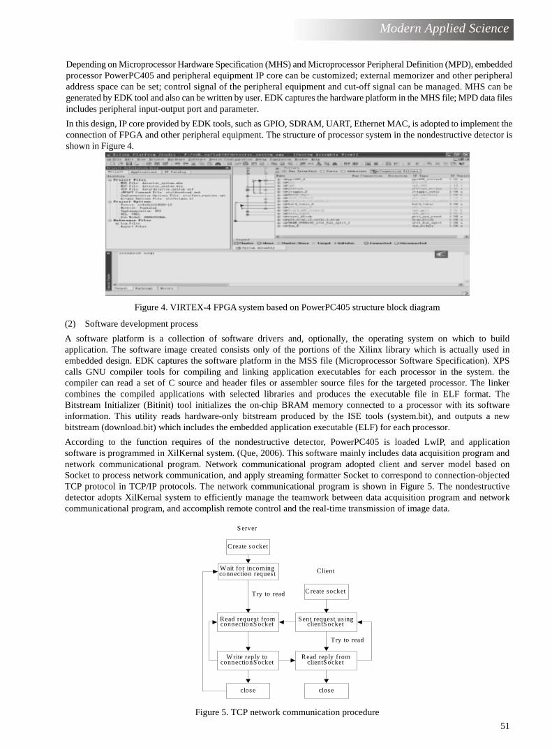
51


Depending on Microprocessor Hardware Specification (MHS) and Microprocessor Peripheral Definition (MPD), embeddedprocessor PowerPC405 and peripheral equipment IP core can be customized; external memorizer and other peripheraladdress space can be set; control signal of the peripheral equipment and cut-off signal can be managed. MHS can begenerated by EDK tool and also can be written by user. EDK captures the hardware platform in the MHS file; MPD data filesincludes peripheral input-output port and parameter.

In this design, IP core provided by EDK tools, such as GPIO, SDRAM, UART, Ethernet MAC, is adopted to implement theconnection of FPGA and other peripheral equipment. The structure of processor system in the nondestructive detector isshown in Figure 4.

Figure 4. VIRTEX-4 FPGA system based on PowerPC405 structure block diagram

(2) Software development process

A software platform is a collection of software drivers and, optionally, the operating system on which to build application. The software image created consists only of the portions of the Xilinx library which is actually used in embedded design. EDK captures the software platform in the MSS file (Microprocessor Software Specification). XPS calls GNU compiler tools for compiling and linking application executables for each processor in the system. the compiler can read a set of C source and header files or assembler source files for the targeted processor. The linker combines the compiled applications with selected libraries and produces the executable file in ELF format. The Bitstream Initializer (Bitinit) tool initializes the on-chip BRAM memory connected to a processor with its software information. This utility reads hardware-only bitstream produced by the ISE tools (system.bit), and outputs a new bitstream (download.bit) which includes the embedded application executable (ELF) for each processor.

According to the function requires of the nondestructive detector, PowerPC405 is loaded LwIP, and application software is programmed in XilKernal system. (Que, 2006). This software mainly includes data acquisition program andnetwork communicational program. Network communicational program adopted client and server model based on Socket to process network communication, and apply streaming formatter Socket to correspond to connection-objected TCP protocol in TCP/IP protocols. The network communicational program is shown in Figure 5. The nondestructive detector adopts XilKernal system to efficiently manage the teamwork between data acquisition program and network communicational program, and accomplish remote control and the real-time transmission of image data.

Create socket

W ait for incoming connection request

Read request from connectionS ocket

Write reply to connectionS ocket

close

C reate socket

Sent request us ing clientSocket

Read reply from clientSocket

close

Try to read

Try to read

Client

S erver

Figure 5. TCP network communication procedure

52


4.1.3 Implementation of Nondestructive detectorX-ray projection light signals are received by photodiode array of X-ray detector card, and a series of electric image signalsare formed. After the electrical signals which are collected and converted by ADC are processed in VIRTEX-4 FPGA, a two-dimensional projection image of the conveyer belt is obtained. The image data are transmitted to network. In Ethernet accesspart, image data are encapsulated according to IP protocol, and then data link layer protocol is used to accomplish theencapsulation of Ethernet frame to this protocol package. Eventually, image data are sent into Ethernet via net interface.

Nondestructive detector includes X-ray detector card, image pixel processor board and DC(digital current) voltage regulator.Image pixel processor board is the key part of the detector, which is composed of ADC, VIRTEX-4 FPGA, reset circuit,system clock circuit, memory circuit, PROM circuit, Ethernet PHY circuit and RS-232 interface, JTAG interface, LVPECL levelinterface circuit. Nondestructive detector structure is shown in Figure 6.

PPC 405

D C M

Systemrese t

JTAGPPCcontroller

PLBSD R AM

OPBGPIO

U AR Tcontroller

EM AC

C rysta l oscilla to r

R ese t circu it

JTAG

SD R AM

I/O

R S232

PH Y

AD C

X-C AR D

Figure 6. Nondestructive detector structure block diagram

(1) System clock

Reference clock is created by external crystal oscillator, and is connected with FPGA internal digital clock management module (DCM) and clock tree by global clock pin of FPGA. DCM supports more than 400MHz clock-out, and supplies a zero delay clock buffer that has 50/50 precision duty ratio. Meanwhile, DCM can accurately control 90, 180, 270 phase-shift ability, accomplishes synthesis of clock signal, and supports to create precise frequency of 24~420MHz. In FPGA interior, DCM centrally distributes the clock signal. The clock output of DCM is set up to system clock of PowerPC, and supplied to PLB, OPB bus arbiter.

(2) External memorizer

PLB bus of PPC405 supports high-speed memory, such as DDR RAM, SDAM etc. OPB bus supports general storage circuit, such as EPROM, SRAM, FALSH and external register etc. In this design, 2 of high-speed synchronous SDRAM (MT48V8M16) are used to be external data memory area of PowerPC405 processor, which have 32 bits data bus width and 32 MB capacity. When compiling MHS document, PLBSDRAM core, where memorizer address bus and data bus width are configured and initial address of memory area is appointed, is chosen to be add. Other setup of the program memorizer is similar as data memorizer besides linking to OPB bus.

(3) Ethernet interface

In FPGA, 10/100/1000M Ethernet MAC core is integrated and externally connected with Marvell Alaska Ethernet PHY(88E1111), which is suitable for the application of IEEE802.3 physical layer. And then it is connected to Ethernet after passing network isolation transformer. When MHS is compiled, Ethernet MAC core is chosen to be added.

(4) RS232 interface

As required, UART controller is integrated in FPGA interior, and is externally connected with RS232. Simultaneously, it links to computer serial that is used to be debugging information output of application program. In MHS, baud rate of serial, data bit width and parity check can be configured.

(5) On-line programmable PROM

FPGA, which is based on gate array, provides programmable recourse to users. Its logic structure is decided by configuration data. The configuration data are loaded to SRAM of FPGA interior by external control circuit or micro-processor. Due to the information stored in SRAM will lose when power-down, FPGA must be reconfigured when power-up. In practical application, 2 of PROM (XC18V04) are used to store configured data stream. FPGA is set to Master Serial mode via jumper. When power-up every time, the configuration data is automatically read from PROM to SRAM, and internal structure mapping is came true.

(6) JTAG port

The FPGA and PROM can be configured though JTAG port. When PowerPC is embedded in VIRTEX-4 FPGA,

application code can be also downloaded and debugged. For the convenience of software code debugging, 4 of general

I/O pins can also be appointed on FPGA besides special configured pins TCK, TMS, TDO and TDI in the FPGA. In

53


addition, JTAG interface internally connected with PowerPC kernel is to configure and debug PowerPC kernel, and tracedebug software code. In this module, software code can be singly downloaded to PowerPC kernel and debug software inkernel. When FPGA is configured via JTAG pins, the notice is that JTAG configuration pin would better connect with pull-up resistor and INIT pin would better connect to earth as configuration period.

4.2 PC software designGeneral frame of developing image process software is set up in WINXP/WIN2000 platform by applying C#.NET. Imageprocess algorithm of conveyor belt is researched, and image processing software of conveyor belt is programmed.

4.2.1Image processing algorithm of conveying belt

Image processing algorithm of conveyor belt is used in the software development of image processing. (Roziere, 1989).Image processing algorithm of nondestructive detection system includes:

(1) Standardization method

Each pixel is adjusted in order to reduce noise adding of channel, and gain difference is eliminated that is caused byunevenness of crystal, coupling between crystal and photodiode or photodiode itself. Each pixel is adjusted by reapplyingthe equation:

Iiout=Gic (Iiraw-Oic+Ob/Gic) (6)

Some variables and constants are listed as follows:Iiout: standardization output signal of pixel i;Gic: gain corrected value;Iiraw: actual pixel value;Oic: bias corrected value;Ob: bias line value.

(2) Grey enhancement

Grey enhancement processing is to use grey transform technique to improve image quality by improving grey change ofimage. In some cases, grey distribution range of image just centralized in narrower area that causes worse contrast andvague outline of image. At that time, the image grey distribution can be extended to 256 grey degree (0~255) by lineartransform in order to improve entire contrast and resolution of image. Assumed that grey distribution arrange of originalimage is A1-A2, the equation of transformation is g(x, y)=255/(A2-A1)[f(x,y)-A1]. In addition, due to proper nonlinear greytransform (such as logarithm, exponent), a target of grey arrange in image can be excel.

(3) Edge sharpening

Sharpening is to emphasize image contour and make image clear and legible. Essence of sharpening is high-pass filteringtechnique. Image sharpening can be implemented by template operation (operator). Choosing property template can accom-plish edge sharpening, boundary detection, feature extraction and smoothed filter and so on.

(4) Image inversion

According to the detection theory of X-ray, X-ray passing steel wire are less than surrounding colloid matter, so imagesignal is relatively weak and image is relatively dark. Image hue of X-ray is inversed to make shown image fit observationhabit of detection personnel. Assumed that grey values of pixel point before and after inversion are respectively f (x, y), g(x, y), the inversion equation is: g(x,y)=255-f(x,y).

In development of software, a lot of methods will be used, such as nonlinear median filtering, edge detection, discreteFourier transform and inverse transform, fast Fourier transform (FFT) and inverse transform etc.

4.2.2Image processing software of conveyor belt

The development of conveyor belt image processing software consists of dynamic display module, defect detectionmodule, data management module, and image processing module and so on.

Dynamic display module mainly completes initialization of detector and show-card, and accomplishes detection imagesdynamic display, capture, reconstruction, Zoom-in and roaming and so on.

Defect detection module completes fuzzy recognition algorithm based on image space character (space contrast and spacevariance), which is to be defect detection algorithm. Initially, advanced image processing method is adopted to make placeand defect more extrusive and striking, and then depending on automatic identification system of computer, quantitativeevaluation, hierarchical classification and qualified judgment system of defect is constructed. Artificial Intelligence algo-rithm is introduced.

Data management module manages detected image data, and reasonably sets database and stores according to differentjoint control numbers or failure numbers and different collective times. Simultaneously, inquire, browsing and modificationof database is supplied.

54


Image processing module uses digital image processing technique to enhance contrast and definition of image, aiming atdefinition enhancement algorithm, such as internal geometric rectification, grey transform, pseudo color. Diagnostic areaprefabricates plot functions toolbox, measurement toolbox and text editor. By using it, users can increase necessaryassistant information on the images; simultaneously, users are allowed to store data and share dynamic data stream throughinternet.

6.Conclusion

In this paper, X-ray detection theory is used to design nondestructive detection system for high-speed running conveyor belt with steel wire ropes. At the case that the speed of conveyor belt is 4.3m/s, nondestructive detection system implements high-speed detection and static running, which is eligible for design requirement. This detection system accomplishes remote control and network transmission of image data, and improves automatically degree of nondestructive detection system. Furthermore, staff can be far from radiant source environment, and it is easy to achieve radiant protection and personnel safety.

References

Cheng, Hong, Gao, yulin & Zhao, Shujing. (1997). A X-ray Non-destructive Test System for Mine Conveyer Belt. HighTechnology Letters. Vol.3, No.1, June, 26~29.

Gao, Zhonglin & Wang, Kaiyuan. (1991). Photoelectric Devices. Nanking: Publishing House of Southeast university.

Getting Started with EDK. (2003). XILINX.

Jussi Koskinen. (2004). LDA Technology Today Possibilities in the Future. Proc. CT & 3D Imaging Conference.132~137.

Klug, H.P. & Alexander, L.E.. (1974). X-ray Diffraction Procedures for Polycrystalline and Amorphous Materials.

PowerPC Processor Reference Guide. (2003). XILINX.

Que, Dashun & Wang, Jintao. (2006). Implementation of LwIP in the μ c/OS-II. Ship Electronic Engineering. Vol.26,No.4, 89~91.

Roziere B M et al. (1989). High Resolution Solid State Linear Detector for X-ray Digital Imaging, Non-Destructive Testing, Proc. 12th World Conference. 705.

Figure 7. The image collected by nondestructive detector

Figure 8. The image processed by image processing software

Vol. 1, No. 3

September 2007

55


Intersectant Possibilities of Linguistics and cosmography

Xiang Li

The First Senior High School of He Gang City, Heilongjiang 154101, China


Abstract

In this article, you will see an attempt about intercrossing of linguistics and cosmography bsaed on the following hypothesis: all the letters (symbols) information can be regarded as elements in the same set.

Keywords: Letters, Exhaustion method, Cosmography, Extending, Educational system

We can suppose that the people had assumed the idea that every letter or symbol has different concepts. The word is composed of letters, and the sentence is composed of words, and the article is composed of sentences, and the information expresses the article. If we arrange letters or symbols in arrangements as more as possible (that is the exhaustion method), so, what would associations exist among them? What would characteristics exist in this set? How would people deal with so much information if necessary? What would all these things imply?

1. Structure

The probability of any element in this set we get should be same, and there are some of these elements which express the idea and opinion. Therefore, the probability of all ideas and opinions that people can receive is same, though this sort of probability is very small. That probability is based on the following description: if one sort of idea or opinion can “be described by the letters” and “can be understood by people in the limited time (which is the hypothesis in the following text)”, so “these letters can not be limitless”, and the premise is that the purpose must be pure. So how to judge these opinions are correct? The perfect opinion is that there must have conclusive evidences and correct logic reasoning and reasonable hypothesis.

The elements in this set are associated, and this relation is multifarious. So all elements will form a network with complex structure and the complex degree of the network is decided by the imagination. Therefore, whatever is correct, whether we can say that “all things people had create since the letters where born are only the part nodes and the associations among nodes?”

Here, according the above thinking method, except for the elements what the thinking method possesses by itself, all the surplus elements can be discarded, and the obvious reason is that we can obtain everything by this method. So, if we suppose that all problems have the corresponding answers which can be described by language, whatever there are so complex relations between problems and answers, this is an automatic system. The probabilities which exceed the range can only be described. We can obtain those existing answers because they are reasonable.

In fact, this article utilizes the thinking method of the anthropic principle. It is obvious that there are many such similar examples. For example, “…a similar situation is the thinking science, and people must use the thinking when they study the thinking science. It is very difficult to separate the principal part and the object, and this is the sign of mature science. Naturally, scientists should shoulder heavy responsibilities (Du, 2006, p19).” The other situation is about the time. When people discuss the time, we must admit that the background of the affair of “discussing the time” is just the time itself. And one of these similar examples is the origin of this article with 1320words.

Whether this sort of thinking method can be extended to those information carriers such as picture and voice? Thisarticle only takes the picture as the example which meaning is just same as the description in the following picture.

(If this Paragraph can be regard as a illustration)

It is hard to say what the illustration is? Picture? Or words? If we regard this illustration as a picture.Pictures are formed of pixels but tis picture have some featwes. Such as, the patterns are formed of pixels is seems like a kind of symbol called English word. But in the view of words, all of these symbols are not the real words.(in the strict sense there are some Syntax mistakes)it can be discemed by readers. The active in your mind of you "from you seen this picture to have been read this sentence" is the best demonstration.

56

Science News

(The contents of the above picture:

It is difficult to explain what the picture is. Is it picture or letter?

As viewed from picture, picture is composed of pels, but this picture has some characters. For example, the picture which is composed of pels resembles one kind of symbol, which called Chinese characters.

As viewed from letter, all this doesn’t comply with strict writing standards, so it can not be called the formal letters.

But as viewed from readers, they can identify this as Chinese characters. The thinking activity since your first sight seeing this picture to completing this paragraph is the best explanation.)

Therefore we can get the conclusions: part picture can be identified as letters, but these pictures seem to accord with some certain special rule which is not clear at present. The only point which can be assured is that if this rule “can be described by letters”, and “can be understood in the limited times by people”, and “is in the purest purpose”, it must be in the “network” and has “various associations” with other elements (it can help to search faster and conform the position in “network”). The similar method seems to can be used in other information transfer (if people don’t doubt the self ability of the language).

As a special example, whether the theory which describes everything in the universe takes the coequal probability?

“Any physical theory is only a sort of hypothesis and is only temporary, and you can not prove it forever (Stephen, 2006,pp.10-11)”. So we can suppose that: there are final truths which restrict everything in faith, and what people can do is to approach it as illimitably as possible. And it must not fulfill any one request of hypothesis mentioned in the above paragraphs, thus we can think the cumulation of complex degrees since science come forth can be regarded as the increase of the word count of papers and this sort of increase will be continued.

2. Computation

The recent new development of quantum informatics seems to support the opinion that “the Moore’s Law is not the strict physical law, it is the law about human creativity and faith, and it must comply with the physical law (Zhang, 2007, pp.10-11)”. That is to say, the operation velocity of every processor is limited such as the velocity of light.

To reduce the work of computation, we can look for the “symbol” which is embodied in the topic and is not visual and can be deleted, affixed or copied. Except for the effective computer, there seems to have no other methods to process so hugeness data. For the sake of achieving the effectiveness and the computer can identify the “symbol” embodied by the topic, we need the technology familiar to the artificial intelligence. The point which needs explanation is that the technology which this work needs be discussed more or less, because the result of this work is unknown, and people are not likely to exactly know what suddenness will happen before the computer achieve the result, thus it is most possibleto endow wisdom with the moral concept (if it is necessary).

3. Conclusions

The affair of “Babel” seems not bad to people (most interpretations thought this at least), anyway, there is one point can be confirmed: Yahveh had indelible contribution to the linguistics (whatever His first thought is). But there is one fact ignored, i.e. people have ceaseless impetus to discover the truths and innovate to opinions of the world (including the language), and He becomes aware of this and conceal the final answer in some certain corner. I think there must be the following words in that corner:

“We define the education as that the human wisdom will not deviate the aim, and the so-called education is the surplus skills after you forget what all the contents you have learned in the school”, said by Albert Einstein.

References

Du, Xinxin & Wu, Zhongchao. (2006). Create Something Out of Nothing: Stephen Hawking and “A Briefer History of Time”. Hunan Science and Technology Press. p.19.

Stephen Hawking & Leonard Mlodinow, interpreted by Wu, Zhongchao. (2006). A Briefer History of Time(tradeedition). Hunan Science and Technology Press. pp.10-11.

Zhangjian. (2007). The quantum technology saves the Moore’s Law: our scientists renovate the world’s record in this area. Computer Fans Magazine. July, 2007. pp.10-11.

Modern Applied Science, ISSN 1913-1844, Vol. 1, No. 3 ...

Documents

Transcript of Modern Applied Science, ISSN 1913-1844, Vol. 1, No. 3 ...