![NERC€¦Translate this page%PDF-1.6 %âãÏÓ 8997 0 obj > endobj 9160 0 obj >/Filter/FlateDecode/ID[1BDAB6F71BBECC41B6339286B8577871>7EDA50638D48DB43AC7B19395C6599EC>]/Index[8997](https://static.fdocuments.in/doc/165x107/5adab2a17f8b9a6d7e8d0990/translate-this-pagepdf-16-8997-0-obj-endobj-9160-0-obj-filterflatedecodeid1bdab6f71bbecc41b6339286b85778717eda50638d48db43ac7b19395c6599ecindex8997.jpg)
Collision Detection in Wireless Sensor Networks … and Information Science; Vol. 8, No. 3; 2015...
38
Computer and Information Science; Vol. 8, No. 3; 2015 ISSN 1913-8989 E-ISSN 1913-8997 Published by Canadian Center of Science and Education 13 Collision Detection in Wireless Sensor Networks Through Pseudo-Coded ON-OFF Pilot Periods per Packet: A Novel Low-Complexity and Low-Power Design Technique Fawaz Alassery 1 , Walid Ahmed 1 , Mohsen Sarraf 1 & Victor Lawrence 1 1 Electrical and Computer Engineering Department, Stevens Institute of Technology, Hoboken, New Jersey, USA Correspondence: Fawaz Alassery, Electrical and Computer Engineering Department, Stevens Institute of Technology, Hoboken, New Jersey, 07030, USA. Tel: 120-1912-7162. E-mail: [email protected] Received: May 1, 2015 Accepted: May 17, 2015 Online Published: May 21, 2015 doi:10.5539/cis.v8n3p13 URL: http://dx.doi.org/10.5539/cis.v8n3p13 The research is financed by Electrical and Computer Engineering Department, Stevens Institute of Technology, Hoboken, NJ, USA and College of Computers and Information Technology, Taif University, Saudi Arabia. Abstract Sensor nodes in Wireless Sensor Networks (WSNs) operate with limited power resources such as small batteries which are difficult to be either recharged or replaced in some environments when depleted. Power consumption represents one of the most constraints impact the design of WSNs, leading to various protocols and algorithms aimed at minimizing the power consumption and extending batteries' lifetime. Sensor nodes in WSNs transmit their periodic packets continuously to central nodes (receivers) which are responsible for decoding packets and transmitting them to other communication networks. In addition, sensors usually follow various MAC strategies which allow accessing to wireless communication channels. However, sensors may attempt to access the wireless channels at the same time, potentially, leading to collisions among multiple nodes. In fact, central nodes in WSNs most often consume a large amount of power due to the necessity to decode every received packet regardless of the fact that the transmission may suffer from packets collision which impede the network performance. Therefore, in the receiver side of WSNs current collision detection mechanisms have largely been revolving around direct demodulation and decoding of received packets and deciding on a collision based on some form of parity bits in each packet for error control. From information theoretic prospective full decoding of received packets with error control bits at central nodes can achieve an efficient usage of network capacity, however, such an approach represents a major burden on power-constrained sensors. This drawback comes from the need to expend a significant amount of energy and processing complexity at sink nodes in order to fully-decode a packet, only to discover the packet is illegible due to a collision. In this paper, we propose a more practical power saving approaches which achieve a significant power saving with low-complexity at the expense of low throughput losses. Based on studying the statistics of received packets, central nodes can make a fast decision to detect a collision without the need for full-decoding of the whole received packets. Our novel approaches not only reduces processing complexity and hence power consumption, but it also reduces the delay incurred to detect a collision since it operates on only a small number of IQ samples in the beginning of a received packet. In such a paradigm, our approaches operate directly at the output of the receiver’s Analog-to-Digital-Converter (ADC) and eliminate the need to pass the corrupted packets through the entire demodulator/decoder line-up. The performance gain of our proposed approach is illustrated through the comparison between the computational complexity of our Statistical Discrimination (SD) approaches and some existing Full Decoding (FD) algorithms (note 1). Our results show that the SD approaches has significant power savings and low computational complexities over existing FD algorithms with low False-Alarm and Miss probabilities, which qualify our SD approaches to be considered as reliable collision detection mechanisms in WSNs. We also show how to tune various design parameters in order to allow a system designer multiple degrees of freedom for design trade-offs and optimization. Keywords: low computational complexity, collisions detection algorithm, pseudo-coded pilot periods, WSN’s protocols, low power WSN’s protocols
Transcript of Collision Detection in Wireless Sensor Networks … and Information Science; Vol. 8, No. 3; 2015...

Computer and Information Science; Vol. 8, No. 3; 2015 ISSN 1913-8989 E-ISSN 1913-8997
Published by Canadian Center of Science and Education
13
Collision Detection in Wireless Sensor Networks Through Pseudo-Coded ON-OFF Pilot Periods per Packet: A Novel
Low-Complexity and Low-Power Design Technique
Fawaz Alassery1, Walid Ahmed1, Mohsen Sarraf1 & Victor Lawrence1 1 Electrical and Computer Engineering Department, Stevens Institute of Technology, Hoboken, New Jersey, USA
Correspondence: Fawaz Alassery, Electrical and Computer Engineering Department, Stevens Institute of Technology, Hoboken, New Jersey, 07030, USA. Tel: 120-1912-7162. E-mail: [email protected]
Received: May 1, 2015 Accepted: May 17, 2015 Online Published: May 21, 2015
doi:10.5539/cis.v8n3p13 URL: http://dx.doi.org/10.5539/cis.v8n3p13
The research is financed by Electrical and Computer Engineering Department, Stevens Institute of Technology, Hoboken, NJ, USA and College of Computers and Information Technology, Taif University, Saudi Arabia.
Abstract
Sensor nodes in Wireless Sensor Networks (WSNs) operate with limited power resources such as small batteries which are difficult to be either recharged or replaced in some environments when depleted. Power consumption represents one of the most constraints impact the design of WSNs, leading to various protocols and algorithms aimed at minimizing the power consumption and extending batteries' lifetime. Sensor nodes in WSNs transmit their periodic packets continuously to central nodes (receivers) which are responsible for decoding packets and transmitting them to other communication networks. In addition, sensors usually follow various MAC strategies which allow accessing to wireless communication channels. However, sensors may attempt to access the wireless channels at the same time, potentially, leading to collisions among multiple nodes. In fact, central nodes in WSNs most often consume a large amount of power due to the necessity to decode every received packet regardless of the fact that the transmission may suffer from packets collision which impede the network performance. Therefore, in the receiver side of WSNs current collision detection mechanisms have largely been revolving around direct demodulation and decoding of received packets and deciding on a collision based on some form of parity bits in each packet for error control. From information theoretic prospective full decoding of received packets with error control bits at central nodes can achieve an efficient usage of network capacity, however, such an approach represents a major burden on power-constrained sensors. This drawback comes from the need to expend a significant amount of energy and processing complexity at sink nodes in order to fully-decode a packet, only to discover the packet is illegible due to a collision. In this paper, we propose a more practical power saving approaches which achieve a significant power saving with low-complexity at the expense of low throughput losses. Based on studying the statistics of received packets, central nodes can make a fast decision to detect a collision without the need for full-decoding of the whole received packets. Our novel approaches not only reduces processing complexity and hence power consumption, but it also reduces the delay incurred to detect a collision since it operates on only a small number of IQ samples in the beginning of a received packet. In such a paradigm, our approaches operate directly at the output of the receiver’s Analog-to-Digital-Converter (ADC) and eliminate the need to pass the corrupted packets through the entire demodulator/decoder line-up. The performance gain of our proposed approach is illustrated through the comparison between the computational complexity of our Statistical Discrimination (SD) approaches and some existing Full Decoding (FD) algorithms (note 1). Our results show that the SD approaches has significant power savings and low computational complexities over existing FD algorithms with low False-Alarm and Miss probabilities, which qualify our SD approaches to be considered as reliable collision detection mechanisms in WSNs. We also show how to tune various design parameters in order to allow a system designer multiple degrees of freedom for design trade-offs and optimization.
Keywords: low computational complexity, collisions detection algorithm, pseudo-coded pilot periods, WSN’s protocols, low power WSN’s protocols
www.ccsenet.org/cis Computer and Information Science Vol. 8, No. 3; 2015
14
1. Introduction
Wireless Sensor Networks (WSNs) have become increasingly popular due to their various applications. WSNs nodes are usually deployed in remote areas to perform their functions. They mainly use broadcast communication and the network topology can change due to the fact that some nodes may be prone to fail. One of the key challenges in wireless sensor design is power consumption, since the nodes have limited power resources as they typically operate off of batteries that are difficult to replace or recharge (Kori, Angadi, Hiremath and Iddalagi,2009) (Y. Shang, 2014). Therefore, a considerable amount of research in WSNs has focused on power saving techniques including the proposal of various power-efficient designs of electronic transceiver circuitry (Zorzi and Rao,2004) and power-efficient Medium Access Control (MAC) protocols (Karapistoli, Stratogiannis,Tsiropoulos and Pavlidou,2012).
The need to extend the lifetime of sensors is a key challenge in designing current WSNs. In the literature, power conservation algorithms play very important role in order to extend the lifetime of WSN nodes, where typically such algorithms attempt at saving power by applying the power saving technique at either the transmitter or the receiver side. For example, using a strong error Correcting Code (ECC) at the transmitter results in more reliable receptions with low Signal-to-Interference-plus-Noise Ratio (SINR). However, this comes at the price of increasing the processing overhead (hence, also translating into increased power consumption) due to having to decode collision corrupted transmissions before knowing that such transmissions are corrupt, in addition to the high computational complexity that is required for using a strong ECC (Akyildiz,2002). Consequently, in WSNs it is necessary to select appropriate channel coding schemes which simultaneously maintain low complexity and low power consumption for the sensor nodes. In (Chen and Abedi,2011), authors proposed a distributed algorithm for turbo coding/decoding in WSNs. The algorithm is based on using parallel concatenation convolutional codes over a noisy channel. In (Hua,2005), the decoding computational complexity at the receiver in WSNs can be decreased via a proposed Viterbi Algorithm for Distributed Source Coding (VA-DSC). Authors in (Cam,2006) proposed an energy-efficient Multiple Input Turbo (MIT) code for WSNs, the code can be used to reduce the amount of bit transmitted from sensor nodes, leading to power saving and better bandwidth utilization. In addition, in order to save power at the receiver in WSNs, it is necessary to avoid decoding of packets which involve in collisions.
Current decoding algorithms used in WSNs may suffer from high computational complexities and power consumptions which affect the network performance. In addition, one of the main sources of overhead power consumption in WSNs is collision detection. When multiple sensors transmit at the same time, their transmitted packets collide at the central node (the receiver) (Miranda, Gomes, Abrishambaf, Loureiro, Mendes, Cabral and Monteiro,2014). Authors in (Jun Peng et al,2007) use out of band control channel to indicate the transmission status (i.e. active state) for sensors which have packets ready to be transmitted. Sensors sense the control channel to detect collision. However, such technique is not accurate to detect collisions that may occur at the receiver. In addition, current collision detection mechanisms have largely been revolving around direct demodulation and decoding of received packets and deciding on a collision based on some form of a frame error detection mechanism, such as a CRC check. The obvious drawback of full decoding of a received packet is the need to expend a significant amount of energy and processing complexity in order to fully-decode a packet, only to discover the packet is invalid and corrupted due to collision. So, decoding of corrupted packets becomes useless and provides the main cause of unnecessary power consumption. In this paper we pose the following questions: Can we propose power-efficient techniquse to detect packets’ collisions at the receiver side of WSNs without the need for full-decoding of the received packet? Further, can we eliminate the need to pass the corrupted packets through the entire demodulator/decoder? To answer these questions we propose suite of novel, yet simple and power-efficient approaches to detect a collision without the need for full-decoding of the received packet. Our novel approach aims at detecting collision through fast examination of the signal statistics of a short snippet of the received packet via a relatively small number of computations over a small number of received IQ samples. Hence, operating directly at the output of the receiver’s analog-to-digital-converter (ADC) and eliminating the need to pass the signal through the entire demodulator/decoder line-up. Figure 1 illustrates where we apply our proposed approaches. In addition, we present a complexity and power-saving comparison between our novel Statistical Discrimination (SD) approach and conventional Full-Decoding (FD) approaches (i.e. for select coding schemes) to demonstrate the significant power and complexity saving advantage of our approaches. Accordingly, our novel SD approaches have the following advantages:
1. The SD approach not only reduces processing complexity and hence power consumption, but it also reduces the latency incurred to detect a collision since it operates on only a small number of samples - that may be chosen to be in the beginning of a received packet - instead of having to buffer and process the
www.ccsenet.org/cis Computer and Information Science Vol. 8, No. 3; 2015
15
entire packet as is the case with a Full-Decoding (FD) approaches.
2. The SD approaches operate directly on the (random) data, i.e., the received packet as is.
3. With a relatively short measurement period, the SD approach can achieve low False-Alarm and Miss probabilities, which qualify it to be considered as a reliable collision detection mechanism at the receiver side of WSNs.
4. The SD approaches can be tuned over various design parameters in order to allow a system designer multiple degrees of freedom for design trade-offs and optimization.
The remainder of this paper is organized as follows. Section 2 describes our system. In section 3, we explain our proposed SD approaches. In section 4, we evaluate the power saving and system throughput based on our SD proposed approaches. In addition, we compare the computational complexity of our SD approaches against commonly used FD algorithms. In section 5, we provided analysis and numerical empirical characterization to provide some quantitative theoretical framework and shed some light on the behavior of the various system factors and parameters involved in our proposed approaches. In section 6, we present performance results, and finally in section 7 we provide the conclusion for this paper.
Figure 1. Block diagram for a receiver’s line-up
2. System Description
Figure 2 depicts an example of a WSN where N interferer sensors and a single desirable sensor are deployed arbitrarily to perform certain functionalities including sensing and/or collecting data and then communicating such information to an access node (a receiver) (note 2). The central node may process and relay the aggregate information to a backbone network or any other communications networks.
At any point in time, multiple packets may accidentally arrive simultaneously and cause a collision. Upon the anticipated time of arrival of packets, the central node will receive packets from a desirable sensor and interferers. A commonly accepted model for packet arrivals, i.e., a packet is available at a sensor and ready to be transmitted, is the well-known Bernoulli-trial-based arrival model, where at any point in time, the probability that a sensor has a packet ready to transmit is .
Upon the receipt of a packet, the central node processes and evaluates the received packet and makes a decision on whether the packet is a collision-free (good) or has suffered a collision (bad). In this paper, we propose suite of fast collision detection techniques where the central node evaluates the statistics of the received signal’s IQ samples at the output of the receiver’s ADC directly using simple discrimination techniques, as will be explained in more detail in the following sections, saving the need to expend power and time on the complex modem line-up processing (e.g., demodulation and decoding). If the packet passes the SD test, it is deemed collision-free and

www.ccsenet.org/cis Computer and Information Science Vol. 8, No. 3; 2015
16
undergoes all the necessary modem processing to demodulate and decode the data. Otherwise, the packet is deemed to have suffered a collision, which in turn triggers the sink node to issue a NACK message per the mechanism and rules mandated by the specific multiple-access scheme employed in the network.
Note that the actual design details and choice of the multiple access mechanism, e.g., slotted or un-slotted Aloha, are beyond the scope of this paper and irrelevant to the specifics of the technique proposed herein.
3. Statistical Discrimination Techniques Description
As mentioned earlier, our proposed approaches are based upon evaluating the statistics of the received signal at the receiver ADC output via the use of simple calculations that are performed on a relatively small portion of the received IQ packet samples. The resulting approaches values are then compared with pre-specified thresholds to determine if the statistics of the received samples reflect an acceptable Signal-to-Interference-plus-Noise Ratio (SINR) from the decoding mechanism perspective. If so, the packed is deemed collision-free and qualifies for further decoding. Otherwise, the packet is deemed to have suffered a collision with other interferer(s) and is rejected without expending any further processing/decoding energy. A repeat request may then be issued so the transmitting sensors to re-try depending on the MAC scheme. In other words, the idea is to use fast and simple
Figure 2. Wireless Sensor Network (WSN) with one desirable sensor, multiple interferer sensors and a central sensor (a receiver)
calculations to determine if the received signal strength (RSS) is indeed due to a single transmitting sensor that is strong enough to achieve an acceptable SINR at the central node’s receiver, or the RSS is rather due to the superposition of the powers of multiple colliding packets, hence the associated SINR is less than acceptable to the decoding mechanism.
Let’s define the kth received signal (complex-valued) IQ sample at the access node as:
k
N
mkmkk nxxy ++=
−
=
1
1,,0
where
QkIkk jyyy ,, += , 1−=j ,
QkIkk jxxx ,,0,,0,0 +=
is a complex-valued quantity that represents the kth IQ sample component contributed by the desired sensor,while
1,...,1 ;,,,,, −=+= Nmjxxx QkmIkmkm
Desirable Sensor
Interferer Sensors
Central Sensor
(Receiver)

www.ccsenet.org/cis Computer and Information Science Vol. 8, No. 3; 2015
17
is the kth IQ sample component contributed by the mth interfering (colliding) sensor. Finally, QkIkk jnnn ,, += is
a complex-valued Additive-White-Gaussian Noise (AWGN) quantity (e.g., thermal noise).
We propose three statistical discrimination (SD) approaches that are applied to the envelope value,
QkIkk yyy ,2
,2 += , of the received IQ samples at the central node as detailed in the following subsections.
3.1 Zero-Power Periods Transmission
The approach is based on zero-power periods transmission per packet as it will be explained further below. For the sake of case study we assume the following:
• Let the transmitted packet be divided into U periods (i.e. slots) where each packet has Z zero-power periods (i.e. power-off slots which carry neither information nor power) and D actual data periods (i.e. power-on slots).
• We form C(U,Z)≥N possible (distinct) zero-power periods combination (i.e. each sensor transmitted packet has its own zero-power periods in locations that can be overlapped with some zero-power periods for packets transmitted from other sensors).
• let is the maximum possible size (or length) of the transmitted packet; = 1,2,…,K. Also, let is the length of the zero power period (note 3); = 1,2,…G, and is the length of the actual data period; =1,2,…,S.
• We assume and represent the lth and hth zero power period and actual data period respectively; l= 1,2,...Z and h= 1,2,...D.
• The absolute power is assumed to be the minimum average power over all packet's slots which have been checked by the central node. It can be defined as:
= min ∑ ∑ , ∑ ∑ | | (1)
where
= , ; i =1,2,…,G
= , ; j=1,2,…,S
Figure 3 shows an example for packets which are transmitted from different sensors where zero-power periods may overlap in their locations.
Figure3. Example of a packet structure for the zero-power periods scheme

www.ccsenet.org/cis Computer and Information Science Vol. 8, No. 3; 2015
18
Upon the receipt of a packet, the central node sweeps all possible zero-power and actual data periods for a packet in order to find the absolute power ( ) and hence compares it with a pre-specified threshold level ( ) that is set based on a desired Signal to Interference plus Noise Ratio (SINR) cut-off assumption ( _ ) (note 4) as will be described in more detail later in subsection 3.4. That is a system designer pre-evaluates the appropriate threshold value that corresponds to the desired _ . If is higher than the threshold value, then the SD approach value reflects a SINR that is less than _ and the packet is deemed not usable, and vice-versa. Accordingly, a “False-Alarm” event occurs if the received SINR is higher than _ but the SD approach erroneously deems the received SINR to be less than
_ . On the other hand, if the SD approach deems the SINR to be higher than _ while it is actually less than
_ , a “Miss” event is encountered.
3.2 Single Pseudo-Coded ON-OFF Pilot Period Transmission
This approach is based on a single pseudo-coded ON-OFF pilot period per packet. Figure 4 depicts a pictorial illustration of the packet structure for the single pilot period scheme.
In the single pilot scheme we assume the following:
• A distinct sequence per sensor. That is, ≠ ; ≠ .
• must have the same duty-cycle (D) for all 1≤ j ≤ N.
• The length of the actual data block is , and the length of the pilot period ( ) is L.
• L is divided into slots which include all zeros slots and all ones slots, i.e., we assume the same ratio of to as well as different ratio (e.g. 30%,40%, etc.). Also, each slot has the same number of samples ( ). Accordingly, we evaluate different length of L based how many and (i.e. L= × ). In our design we try to minimize L as much as possible and ensure the SD approach would still work reliably. For example, we assume =8 slots and =2 samples, so L= 16 samples (It can be tuned as required by a designer).
• The central node is aware of what transmitted period to expect for each sensor.
• We evaluate various "soft" decision percentages (i.e.ℵ) when decoding the pilot period at the central node. We quantify the effect and performance versus different ℵ such as 60%,70% and 90% (It can be tuned as required by a designer).
• The relative power is assumed to be the average power for the actual data block to the average power for the pseudo-coded ON-OFF pilot period. It can be defined as:
= ∑ ∑ (2)
where
= , ; i =L+1,L+2,…, and = , ; j =1,2,…,L
In the single pilot period approach, the central node needs to decode (i.e. through ML detection) the pilot sequence for each received packet and compare it with the pre-stored look-up table (code-book) of all the valid sequences. If the sequence of the decoded pseudo-coded ON-OFF pilot period matchℵ (or more) of any pre-stored sequence, then the received packet is a collision-free packet, and vice versa.
For a collision-free packet and similar to the previous approach, the relative power( ) is compared with a pre-specified threshold value that is set based on _ . If is higher than the threshold value, then the SD approach value reflects a SINR that is less than _ and the packet is deemed not usable, and vice-versa. Accordingly, a “False-Alarm” event occurs if the received SINR is higher than _ but the SD approach erroneously deems the received SINR to be less than
_ . On the other hand, if the SD approach deems the SINR to be higher than _ while it is actually less than
_ , a “Miss” event is encountered.
In the following we show how to decode the single pseudo-coded ON-OFF pilot period through the Maximum Likelihood (ML) detection (note 5). Let the transmitted block be ; k=1,2,…, , +1,…, and the received block be ; k=1,2,…, , +1,…, . As mentioned earlier, the kth received signal (complex-valued) IQ sample at the central node is:

www.ccsenet.org/cis Computer and Information Science Vol. 8, No. 3; 2015
19
k
N
mkmkk nxxy ++=
−
=
1
1,,0
where , is a complex-valued quantity that represents the kth IQ sample component contributed by the desired sensor, while , is the kth IQ sample component contributed by the mth interfering (colliding) sensor. Finally, is a complex-valued Additive White Gaussian Noise (AWGN) quantity. Accordingly, the channel transition probability density function (pdf) P( | ) is:
P( | )= ( . ) exp − , ∑ | | (3)
Hence, ML detection algorithm needs to maximize P( │ ) ,i.e., similar to (3) for all received packets, where
in this case is the vector for the received pilot period, and is the vector for the transmitted pilot period.
Equivalently, ML detector can maximize the log-likelihood function for the pilot period as follows: ∝ P │ = −∑ −
The following procedures implement the ML detection for our proposed single pseudo-coded ON-OFF pilot period approach:
1. Start with k =1.
2. Calculate:
= −∑ −
3. Store . 4. Increment k by one. 5. If k=L+1 go to step 7. 6. Go to step 2. 7. Find the sequence that correspond to the largest and declare it as the detected sequence ( ).
If the sequence matchℵ (or more) of any pre-stored sequence, then the corresponding received packet is declared as a collision free packet. For the collision free packet, is compared with a pre-specified threshold level (i.e. set based on _ ) in order to analyze packet's statistics (i.e. False-Alarm and Miss probabilities).
Figure 4. Example of a packet structure for the single pseudo-coded ON-OFF pilot period

www.ccsenet.org/cis Computer and Information Science Vol. 8, No. 3; 2015
20
3.3 Double Pseudo-Coded ON-OFF Pilot Periods Transmission
In order to improve the system performance as will be described in the following sections, in this approach we propose double pseudo-coded ON-OFF pilot periods per packet. Figure 5 depicts a pictorial illustration of the packet structure for the double pilot period appoach. The approach has the following assumption:
• A distinct sequence per sensor. That is, , ≠ , and , ≠ , ; i ≠ j.
• , and , must have the same duty-cycles (i.e. and respectively) for all 1≤ j ≤ N.
• The length of the actual data block is , the length of the first pilot period ( , ) is , and the length of the second pilot period ( , ) is .
• is divided into slots which include all zeros slots and all ones slots, i.e., we assume the same ratio of to as well as different ratio, e.g., 30%,40%,etc.
• is divided into slots which include all zeros slots and all ones slots, i.e., we assume the same ratio of to as well as different ratio, e.g., 60%,70%,etc.
• Each slot in the first and second pilot period has the same number of samples, i.e., and respectively. Accordingly, we evaluate different length of and based how many , d, and (i.e. = × and = × ). In our design we try to minimize and as much as possible and ensure the SD approach would still work reliably (i.e. short pilot periods). For example, we assume
=8 slots/period, d=7 slots/period, = 2 samples/slot and =3 samples/slot, so =16 samples/period and =21 samples/period. (It can be tuned as required by a designer).
• The central node is aware of what transmitted , and , periods to expect for each sensor.
• We evaluate various "soft" decision percentages when decoding the pilot periods at the central node (i.e. ℵ and ℵ for the first and second pilot periods respectively). We quantify the effect and performance versus different ℵ and ℵ such as 60%,70% and 90% (It can be tuned as required by a designer).
• The relative power is assumed to be the average power for the actual data block to the average power for the pseudo-coded ON-OFF pilot periods. It can be defined as:
= ∑ ∑ ∑ (4)
Where = ; i = +1, +2,…, +
= ; =1,2,…,
= ; = + +1, + +2,…, + +
In the double pilot periods approach, the central node needs to decode (i.e. through Maximum Likelihood (ML) detection) both pilot sequences for each received packet and compare them with the pre-stored look-up table (code-book) of all the valid sequences (i.e. and for the first and second pilot periods respectively). If the sequence of the first decoded pilot period matchℵ (or more) of any pre-stored sequence ( ) and the second decoded pilot period match ℵ (or more) of any pre-stored sequence ( ), then the received packet is a collision-free packet, and vice versa.
For a collision-free packet and as mentioned in previous techniques, the relative power ( ) is compared with the _ . If is higher than the threshold value, then the SD approach value reflects a SINR that is less than _ and the packet is deemed not usable, and vice-versa. Accordingly, a “False-Alarm” event occurs if the received SINR is higher than _ but the SD approach erroneously deems the received SINR to be less than
_ . On the other hand, if the SD approach deems the SINR to be higher than _ while it is actually less than
_ , a “Miss” event is encountered. Miss and False-Alarm probabilities directly impact the overall system performance as will be discussed in the following sections. Therefore, it is desired to minimize such probabilities as much as possible.
www.ccsenet.org/cis Computer and Information Science Vol. 8, No. 3; 2015
21
Figure 5. Example of a packet structure for the double pseudo-coded ON-OFF pilot periods
In the following we show how to decode the double pseudo-coded ON-OFF pilot periods through the Maximum Likelihood (ML) detection. Let the transmitted block be ; k= (1,2,.…, ),( +1,…., + ),( + +1,…., + + ) and the received block be ; k=(1,2,.…, ),( +1,…., + ),( + +1,…., + + ). Hence, ML detection algorithm needs to maximize P( │ ) and P( │ ) for the first and second pilot periods respectively similar to that defined in (3) for all received packets, where in this case is the vector for the first pilot period received by the central node, and is the vector for the first pilot period transmitted by a sensor, is the vector for the second pilot period received by the central node, and is the vector for the second pilot period transmitted by a sensor. Equivalently, ML detector can maximize the log-likelihood function for both pilot periods as follows: ∝ P │ = −∑ −
∝ P │ = −∑ −
The following procedures implement the ML detection for our proposed double pseudo-coded ON-OFF pilot periods approach:
1. Start with =1 and =1.
2. Calculate:
= −∑ − and = −∑ −
3. Store and .
4. Increment and by one.
5. If = +1 and = +1 go to step 7.
6. Go to step 2.
7. Find the sequences that correspond to the largest and and declare them as the detected sequences
(i.e. , and , ). If the sequences , and , match ℵ and ℵ (or more) of any pre-stored sequences and

www.ccsenet.org/cis Computer and Information Science Vol. 8, No. 3; 2015
22
respectively, then the corresponding received packet is declared as a collision free packet. For the collision free packet, is compared with a pre-specified threshold level (i.e. set based on _ ) in order to calculate the False-Alarm and Miss probabilities.
3.4 Threshold Selection
The decision threshold is chosen based on evaluating the False-Alarm and Miss probabilities and choosing the threshold values that satisfy the designer’s requirements of such quantities. For example, we generate, say, a 100,000 Monte-Carlo simulated snapshots of interfering sensors (e.g., 1~30 sensors with random received powers to simulate various path loss amounts) where for each snapshot we compute the SD approach’s value (i.e. ) for the received SINR and compare it with various threshold levels, determine if there is a corresponding False-Alarm or Miss event and record the counts of such events. At the end of the simulations the False-Alarm and Miss probabilities are computed and plotted versus the range of evaluated threshold values, which in-turn, enables the designer to determine a satisfactory set point for the threshold.
4. Power Saving and System Throughput Analysis
To analyze the power saving of our proposed SD system we introduce the following computational complexity metrics:
= S + (5)
= S + (1 − ) (6) In above formulas, S is the number of computational operations incurred in our proposed approaches (anyone of the three proposed approaches), while F is the number of computational operations incurred in a Full-Decoding approaches (FD), and are the probabilities of Miss and False-Alarm events respectively. Hence, represents the computational complexity for the case where the central node makes a wrong decision to fully-decode the received packet (i.e., declared as a collision-free packets) while the packet should has been rejected (i.e., due to collision). On the other hand, is the computational complexity for the case where the central node makes a correct decision to fully decode received packet (note 6).
In addition, and for the comparison purposes, we introduce the following formulae in order to compare the computational complexity saving achieved by the proposed SD approach (i.e. ) over the FD approach (i.e.
):
= + _ (7)
= F (8) In above formulae, and _ are the probabilities of collision and no-collision events respectively. and _ have been obtained via Monte-Carlo simulation as follows: A random number of interfering sensors (maximum of 30 sensors) is generated per a simulation snapshot, where each sensor is assumed to have a randomly received power level at the access node (to reflect a random path loss/location effect). The generation of the interfering sensors is based on a Bernoulli trial model where it is assume that the probability of a packet available for transmission at a sensor (hence the existence/generation of the sensor for the snapshot at hand) is equal to . If the total SINR is found to be worse than the cut-off limit, a collision is assumed and vice-versa. For our numerical example in this section we used = 0.3and _ = 5dB. Also, we typically generate more than 100,000 snapshots in order to achieve a reliable estimate of the collision probabilities. For the aforementioned choices of and
_ , we found the collision probabilities to be = 0.3649 and _ = 0.6351.
4.1 Comparing with Full-Decoding
In order to assess the computational complexity of our SD approaches, we first quantize the SD calculations in order to define fixed-point and bit-manipulation requirements of such calculations. We also assume a look-up table (LUT) approach for the complexity analysis calculation. Note that the number of times the SD approaches need to access the LUT equals the number of IQ samples involved in the complexity calculation. Thus, our SD approaches only need to perform addition operations as many times as the number of samples. Hence, if the number of bits per LUT word/entry is equal to M at the output of the LUT, our SD approaches need as many M-bit addition operations as the number of IQ samples.
As a case-study, we compare the complexity of the three proposed SD approaches with the complexity of FD algorithms assuming a log-MAP algorithm, a Max-log-MAP algorithm and a Soft Output Viterbi Algorithm (SOVA), respectively. These algorithms have been attractive choices for WSNs (Li, Maunder, Al-Hashimi and Hanzo,2013). Authors in (Robertson, Villebrun and Hoeher,1995) measure the computational complexity of
www.ccsenet.org/cis Computer and Information Science Vol. 8, No. 3; 2015
23
log-MAP, Max-log-MAP and SOVA (per information bit of the decoded codeword) based on the size of the encoder memory. It has been shown that for a memory length of , the total computational complexity per information bit for log-MAP, Max-log-MAP and SOVA can be estimated respectively as:
13225MAP-Log +×= λF (9)
17215MAP-Log-Max +×= λF (10)
( ) 161923SOVA +++×= λλF (11)
In contrast, our SD system does not incur such complexity related to the size of the encoder memory. In addition, our SD system avoids other complexities required by a full decoding such as time and frequency synchronization, Doppler shift correction, fading and channel estimation, etc., since our SD scheme operates directly at the IQ samples at the output of the ADC “as is”. Finally, the FD approaches require buffering and processing of the entire packet/codeword while our SD scheme needs only to operate on a short portion of the received packet.
Now let’s compute the computational complexity for our SD approaches. Let’s assume that the IQ ADCs each is D bits. Also, let’s assume a ( )2⋅ operation is done through a LUT approach to save multiplication operations. In addition, let’s also assume that the square-root, ⋅ , is also done through a LUT approach. Hence, each of the 2I and 2Q operations consume of the order of D bit-comparison operations to address the ( )2⋅ LUT. Then, if the output of the LUT is G bits, it follows that we need about G bit additions for an 22 QI + operation. Let’s assume that the ⋅ LUT has G bits for input addressing and K output bits. Then, we need about G+1 bit-comparison operations to address the ⋅ LUT.
Finally, for simplicity, let’s assume that a bit comparison operation costs as
much as a bit addition operation (note 7). Accordingly, the total number of operations needed to computethe ( )22 QI + for one IQ sample is:
( ) 12212 ++=+++ GDGGD (12)
However, our approach is based on calculating the power for the pilot period and the actual data period. So, the total number of operations needed to compute the ( + ) for one IQ sample (E) is:
GDE += 2 (13)
If we assume the IQ over-sampling rate (OSR) to be Z (i.e., we have Z samples per information symbol), then we need about GZ × bit additions to add the Z( + ) values for every information symbol. Hence, for one information symbol, we need a total of:
( ) GZZGD ×+×+2 = ( )ZGD 22 + (14)
Now if we assume an M-ary modulation (i.e., ( )M2log information bits are mapped to one symbol), then the
computational complexity per information bit can be computed as:
( )( )M
ZGDS
2log
22InfoBit/
+= (15)
For example, in order to show the complexity saving of our SD schemes, let’s assume a QPSK modulation scheme (M=4). Also, let’s assume Z=2 (2 samples per symbol), and D = G = 10 bits, which represents a good bit resolution. Also, let’s assume a memory size of 5=λ for the Log-MAP, Max-Log-MAP and SOVA decoders. Using the formulae (9),(10) and (11), it follows the Log-MAP FD algorithm costs 813 operations per an information bit, the MAX-Log-MAP FD algorithm costs 497 operations per an information bit, and the SOVA FD algorithm costs 166 operations per an information bit while our SD approaches based on formula (15) costs only 40 operations per an information bit, which represents an 95%, a 91% and 75% saving on the computational complexity over log-MAP, Max-log-MAP and SOVA algorithms respectively.
In addition, in a no-collision event, the SD approaches check would represent a processing overhead. Nonetheless, our SD approaches still provid a significant complexity saving over the FD approaches as demonstrated by the following example (note 8). Tables 3 in Appendix A shows the probability of Miss and False-Alarm to be 0.0926 and 0.0921, respectively, for the zero-power periods technique, QPSK and a 50 bits measurement period. In addition, table 6 in the in Appendix A shows the probability of Miss and False-Alarm to be 0.0712 and0.0718, respectively, for the single pilot period technique, QPSK, ℵ=70%, and a 50 bits measurement period. Moreover, table 9 in the in Appendix A shows the probability of Miss and False-Alarm to
www.ccsenet.org/cis Computer and Information Science Vol. 8, No. 3; 2015
24
be 0.0313 and0.0315, respectively, for the double pilot periods technique, QPSK, ℵ =ℵ =70%, and a 50 bits measurement period. Now, based on formulae (5) and (6), and (per information bit) for our SD approaches against log-MAP, Max-log-MAP and SOVA algorithms respectively are equal: , = S + = 40 + 0.0926 × 813= 115 Operations per Info Bit , = S + (1− ) = 40 + (1−0.0921) × 813= 778 Operations per Info Bit , = S + = 40 + 0.0712 × 497= 75 Operations per Info Bit , = S + (1− ) = 40 + (1−0.0718) × 497= 501 Operations per Info Bit , = S + = 40 + 0.0313 × 166= 45 Operations per Info Bit , = S + (1− ) = 40 + (1−0.0315) × 166 = 200 Operations per Info Bit
For the comparison purposes between our SD approach and FD algorithms (i.e. the Log-MAP, the Max-Log-MAP and the SOVA respectively), formulae (7) and (8) are used to find the computational complexity when no-collision is detected: , = , + , _ = 115 × 36.49% + 778 × 63.51% = 536 Operations per Info Bit , = = 813 Operations per Info Bit , = , + , _ = 75 × 36.49% + 501 × 63.51% = 345 Operations per Info Bit , = = 497 Operations per Info Bit , = , + , _ = 45 × 36.49% + 200 × 63.51% = 143 Operations per Info Bit , = = 166 Operations per Info Bit
Hence, the complexity savings (in number of operations per information bit) against the Log-MAP, Max-Log-MAP and SOVA becomes respectively as: ∆ , % = ( , − , )/ , = (813 – 536) / 813 = 34.07 % ∆ , % = ( , − , )/ , = (497 – 345) / 497= 30.58 % ∆ , % = ( , − , )/ , = (166 – 143) / 166= 13.85 %
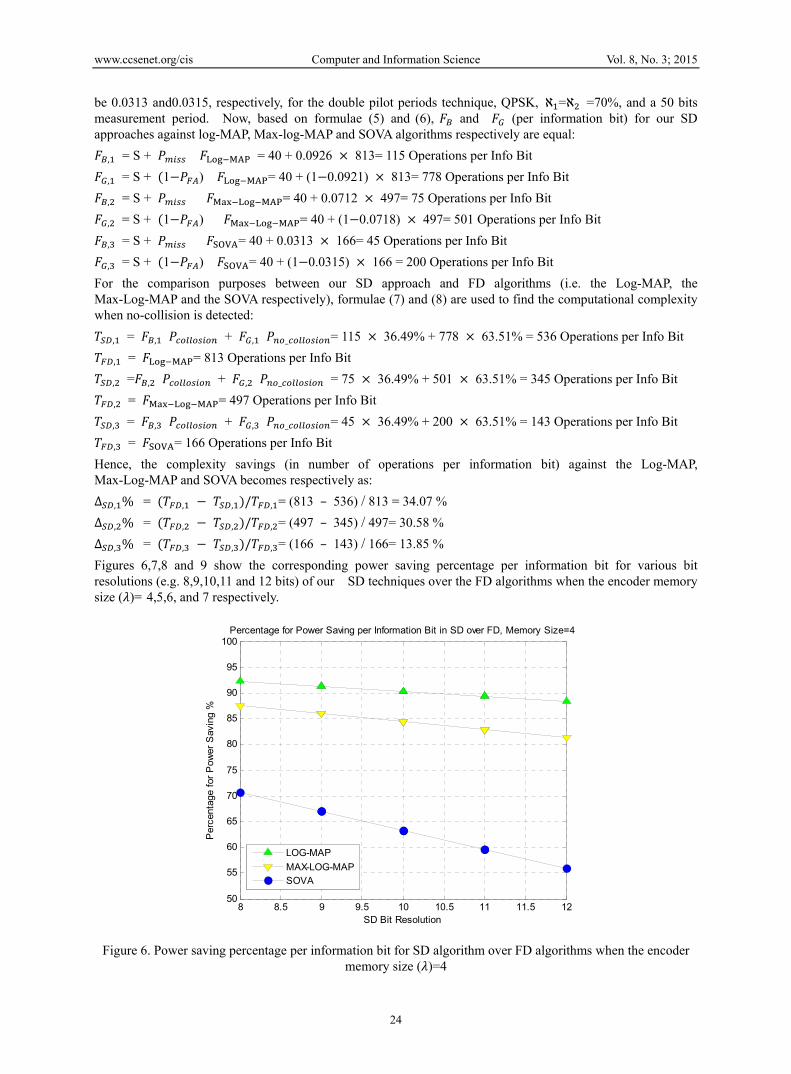
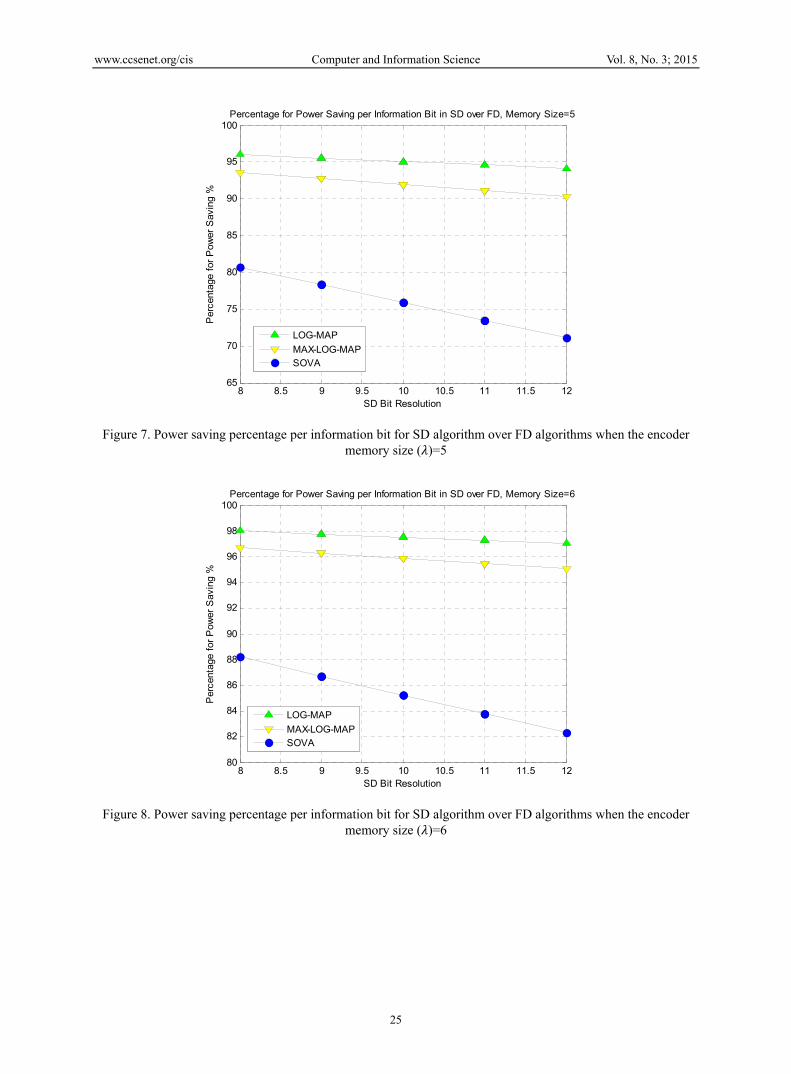
Figures 6,7,8 and 9 show the corresponding power saving percentage per information bit for various bit resolutions (e.g. 8,9,10,11 and 12 bits) of our SD techniques over the FD algorithms when the encoder memory size ( )= 4,5,6, and 7 respectively.
Figure 6. Power saving percentage per information bit for SD algorithm over FD algorithms when the encoder memory size ( )=4
8 8.5 9 9.5 10 10.5 11 11.5 1250
55
60
65
70
75
80
85
90
95
100Percentage for Power Saving per Information Bit in SD over FD, Memory Size=4
SD Bit Resolution
Per
cent
age
for
Pow
er S
avin
g %
LOG-MAP
MAX-LOG-MAPSOVA
www.ccsenet.org/cis Computer and Information Science Vol. 8, No. 3; 2015
25
Figure 7. Power saving percentage per information bit for SD algorithm over FD algorithms when the encoder memory size ( )=5
Figure 8. Power saving percentage per information bit for SD algorithm over FD algorithms when the encoder memory size ( )=6
8 8.5 9 9.5 10 10.5 11 11.5 1265
70
75
80
85
90
95
100Percentage for Power Saving per Information Bit in SD over FD, Memory Size=5
SD Bit Resolution
Per
cent
age
for
Pow
er S
avin
g %
LOG-MAP
MAX-LOG-MAPSOVA
8 8.5 9 9.5 10 10.5 11 11.5 1280
82
84
86
88
90
92
94
96
98
100Percentage for Power Saving per Information Bit in SD over FD, Memory Size=6
SD Bit Resolution
Per
cent
age
for
Pow
er S
avin
g %
LOG-MAP
MAX-LOG-MAPSOVA

www.ccsenet.org/cis Computer and Information Science Vol. 8, No. 3; 2015
26
Figure 9. Power saving percentage per information bit for SD algorithm over FD algorithms when the encoder memory size ( )=7
Note that the above complexity saving calculations, in fact, represent a lower bound on the saving since the above calculations did not take into account the modem line-up operational complexity in order to demodulate and receive the bits in their final binary format properly (i.e., synchronization, channels estimation, etc.).
The performance of our technique can be tuned as desired by a system designer. Appendix A provides performance comparisons for various examples where the system designer may have multiple degrees of freedom for design trade-offs and optimization.
5. Empirical Characterization
In this section, we attempt at empirically characterizing the statistics of various key quantities considered and encountered in this work, in an attempt to shed some light onto the behavior of such quantities and pave the way for some analytic mathematical tractability.
5.1 Statistics of the IQ Signal Envelope
In order to obtain reliable statistics, we have simulated different scenarios that reflect reasonably realistic assumptions (note 9). For example, in our simulations, we assume that packets are generated at the various sensors using a Bernoulli trial model. That is, the probability of a packet available for transmission at a sensor is equal to
. We also generate random number of sensors per a network snapshot that are placed at random locations and distances from the central node in order to reflect various path loss situations (note 12). The individual received sensor and noise components at the access node, as well as the total received signal (the superposition of the sensor received signals plus AWGN) are always normalized properly to reflect the correct SINR assumption.
In general, the parameters covered in this investigation include:
• Number of sensors (note 10).
• level. For our simulations, we typically assumed
= 5dB (note 11).
• Sensitivity (tolerance) around the . That is, if the received SINR is within, for example, 1dB, 1.5dB, −2dB, −10dB or etc. around (5dB), we denote such SINR tolerance level as ∆ .
• Probability of transmission per sensor ( )
• Modulation scheme.
• Measurement duration.
• SD technique choice.
8 8.5 9 9.5 10 10.5 11 11.5 1288
90
92
94
96
98
100Percentage for Power Saving per Information Bit in SD over FD, Memory Size=7
SD Bit Resolution
Per
cent
age
for
Pow
er S
avin
g %
LOG-MAP
MAX-LOG-MAPSOVA

www.ccsenet.org/cis Computer and Information Science Vol. 8, No. 3; 2015
27
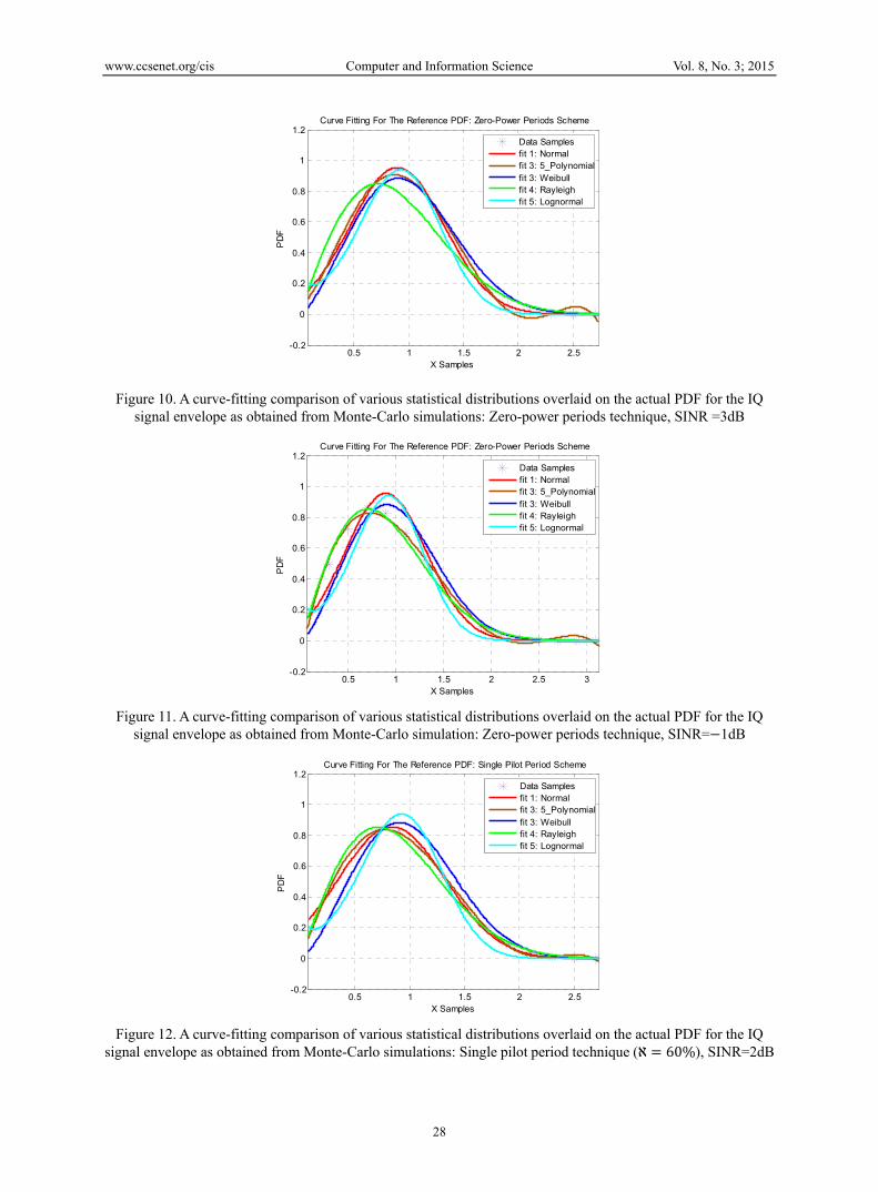
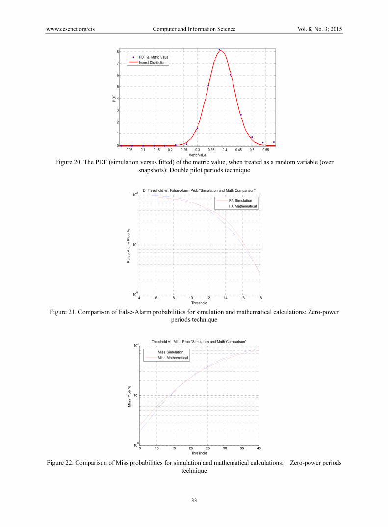
In general, we have found that the Normal (Gaussian) distribution has the closest fit to the actual (simulated) PDF of received signal envelope when SINR ≥ 0dB. For SINR<0dB, however, the Rayleigh distribution seems to be a better fit. We qualify the fitting accuracy of a distribution using the least-mean-square error (LMSE) criterion. Accordingly, the Normal and Rayleigh distributions have exhibited the minimum LMSE in comparison with other distributions as seen in Figures 10 and 11 (such as 5th degree polynomial fit, the Weibull distribution and the Log-normal distribution).
For example, in Figure 10, the normal distribution with mean ( = 0.9525), variance ( = 1.210) resulted in a LMSE = 0.0027 and exhibited the closest fit to the actual (simulated) PDF of the received signal envelope. The choice of parameters for this example has been as follows:
• Maximum number of sensors is 30 (i.e., the number of simultaneous sensors existing in the network per a simulation snapshot is between 2 and 30 sensors).
• = 5dB, SINR= 3dB (∆ = −2dB). • Probability of a packet available for transmission at a sensor is 0.3 (i.e., the Bernoulli trial model
probability is = 0.3). • Modulation scheme is QPSK. • Measurement period is equal to 200 information bits. • Zero-power periods technique.
In Figure 11, the Rayleigh distribution achieved a LMSE = 0.0041 and exhibited the closest fit to the PDF of received signal envelope. Again, the choice of parameters in this figure is assumed as follows:
• Maximum number of sensors is 30.
• = 5dB, SINR= −1dB (∆ = −6dB).
• = 0.3
• Modulation scheme is QPSK.
• Measurement period is equal to 200 information bits.
• Zero-power periods technique.
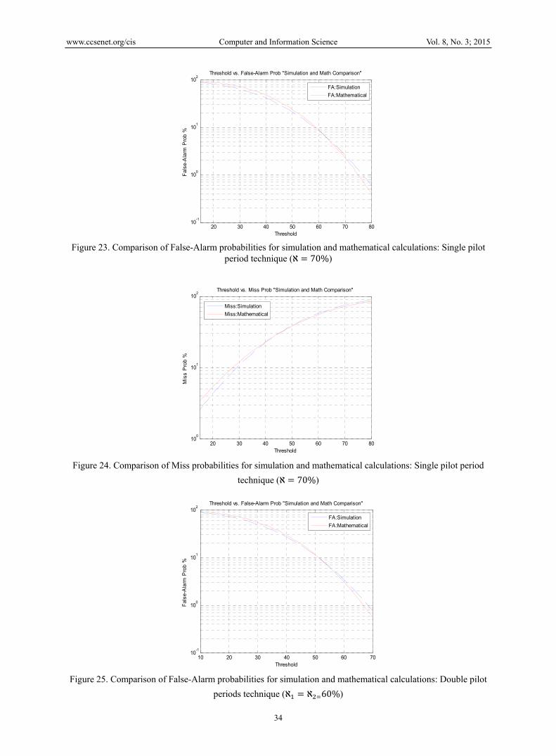
Figures 12 and 13 show similar examples for the single pilot period technique. As shown in Figure 12, the Normal distribution has the closest fit and achieves an LMSE = 0.0134, while in Figure 13 the Rayleigh distribution shows the best fit with LMSE= 0.0521. The parameters are as shown below:
• Maximum number of sensors is 30.
• = 5dB, SINR= 2dB (∆ = −3dB) for Figure 12, while = 5dB, SINR= −3dB (∆ = −8dB) for Figure 13.
• = 0.4.
• Modulation scheme is 8PSK and the measurement period is 100 information bits.
• Single pilot period technique (ℵ = 60%).
Finally, Figures 14 and 15 show corresponding examples for the double pilot periods technique. Again, the Normal and Rayleigh distributions have best fits with LMSE= 0.0030 and LMSE= 0.010, respectively. Our choice of parameters is as follows:
• Maximum number of sensors is 30.
• = 5dB, SINR= 7dB (∆ =2dB) for Figure 14, while = 5dB, SINR= −5dB (∆ = −10dB) for Figure 15.
• = 0.2.
• Modulation scheme is 16PSK.
• Measurement period is 500 information bits.
• Double pilot periods technique (ℵ = ℵ = 70%).
www.ccsenet.org/cis Computer and Information Science Vol. 8, No. 3; 2015
28
Figure 10. A curve-fitting comparison of various statistical distributions overlaid on the actual PDF for the IQ signal envelope as obtained from Monte-Carlo simulations: Zero-power periods technique, SINR =3dB
Figure 11. A curve-fitting comparison of various statistical distributions overlaid on the actual PDF for the IQ signal envelope as obtained from Monte-Carlo simulation: Zero-power periods technique, SINR=−1dB
Figure 12. A curve-fitting comparison of various statistical distributions overlaid on the actual PDF for the IQ signal envelope as obtained from Monte-Carlo simulations: Single pilot period technique (ℵ = 60%), SINR=2dB
0.5 1 1.5 2 2.5-0.2
0
0.2
0.4
0.6
0.8
1
1.2
X Samples
PD
F
Curve Fitting For The Reference PDF: Zero-Power Periods Scheme
Data Samplesfit 1: Normalfit 3: 5_Polynomialfit 3: Weibullfit 4: Rayleighfit 5: Lognormal
0.5 1 1.5 2 2.5 3-0.2
0
0.2
0.4
0.6
0.8
1
1.2
X Samples
PD
F
Curve Fitting For The Reference PDF: Zero-Power Periods Scheme
Data Samplesfit 1: Normalfit 3: 5_Polynomialfit 3: Weibullfit 4: Rayleighfit 5: Lognormal
0.5 1 1.5 2 2.5-0.2
0
0.2
0.4
0.6
0.8
1
1.2
X Samples
PD
F
Curve Fitting For The Reference PDF: Single Pilot Period Scheme
Data Samplesfit 1: Normalfit 3: 5_Polynomialfit 3: Weibullfit 4: Rayleighfit 5: Lognormal

www.ccsenet.org/cis Computer and Information Science Vol. 8, No. 3; 2015
29
Figure 13. A curve-fitting comparison of various statistical distributions overlaid on the actual PDF for the IQ
signal envelope as obtained from Monte-Carlo simulations: Single pilot period technique (ℵ = 60%),
SINR= −3dB.
Figure 14. A curve-fitting comparison of various statistical distributions overlaid on the actual PDF for the IQ
signal envelope as obtained from Monte-Carlo simulations: Double pilot periods technique (ℵ = ℵ = 70%),
SINR =7dB.
Figure 15. A curve-fitting comparison of various statistical distributions overlaid on the actual PDF for the IQ signal envelope as obtained from Monte-Carlo simulations: Double pilot periods technique (ℵ = ℵ = 70%),
SINR= −5dB
0.5 1 1.5 2 2.5 3-0.2
0
0.2
0.4
0.6
0.8
1
1.2
X Samples
PD
F
Curve Fitting For The Reference PDF: Single Pilot Period Scheme
Data Samplesfit 1: Normalfit 3: 5_Polynomialfit 3: Weibullfit 4: Rayleighfit 5: Lognormal
0.5 1 1.5 2 2.5-0.2
0
0.2
0.4
0.6
0.8
1
1.2
X Samples
PD
F
Curve Fitting For The Reference PDF: Double Pilot Periods Scheme
Data Samplesfit 1: Normalfit 3: 5_Polynomialfit 3: Weibullfit 4: Rayleighfit 5: Lognormal
0.5 1 1.5 2 2.5 3-0.2
0
0.2
0.4
0.6
0.8
1
1.2
X Samples
PD
F
Curve Fitting For The Reference PDF: Double Pilot Periods Scheme
Data Samplesfit 1: Normalfit 3: 5_Polynomialfit 3: Weibullfit 4: Rayleighfit 5: Lognormal
www.ccsenet.org/cis Computer and Information Science Vol. 8, No. 3; 2015
30
5.2 Statistics of the SD Metrics
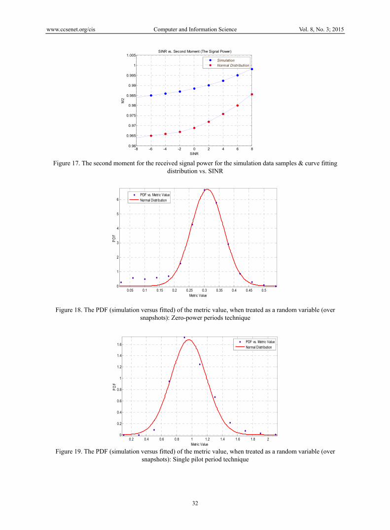
In general, the ensemble (overall) averages (mean) of the first moment of the IQ envelope of the received signals, as well as the second moment (i.e., the power of received signals) are functions of the received SINR. In the following, we plot the ensemble averages of the first and second moments (in Figures 16 and 17 respectively) of the IQ envelope quantity viruses the corresponding first and second moment values that correspond to the best fitting distribution (i.e., Normal and Rayleigh PDFs as pointed out above). The parameters in Figures 16 and 17 are assumed as follows:
• Maximum number of sensors is 30. • = 5dB, SINR= [−8dB, 8dB]. • = 0.2. • Modulation scheme is QPSK. • Measurement period is 100 information bits. • Single pilot period technique.
In addition, we have found that the normal distribution has the best fit to the simulated PDFs for the zero-power periods, the single pilot period and the double pilot periods techniques. The corresponding normal curve fittings are shown in Figures 18, 19 and 20 for the zero-power periods, the single pilot period and the double pilot periods techniques respectively. These figures have the same parameters of figures 10, 12 and 14 respectively.
Based on the normal PDF fit (LeBlance,2004), one can calculate the False-Alarm and Miss probabilities as follows. If we assume a pre-defined threshold level( ), then it can be shown that:
= ( > |( = ; > )
= ( )√ ( ( ))( ) dx (16)
= ( < |( = ; < )
= ( )√ ( ( ))( ) dx (17)
It should be noted that direction of the SD approaches threshold-crossing versus SINR, i.e., whether the SD approaches values ( ) being greater than or less than the threshold are an indicative of SINR being greater than or less than the cut-off SINR (i.e., a collision or not event) is easily seen by inspecting the numerical behavior of the the SD approaches, which has been strictly consistent. Also, it should be noted that as indicated by Equations (16) and (17) above, the means (and variances) of the curve-fitting Gaussian PDFs used in approximating the False-Alarm probability versus the Miss probability are of generally different values since these PDFs are computed under disjoint conditions (i.e., SINR greater than or less than the cut-off), as demonstrated, for example, in Figures (16) and (17). Clearly, and are not complimentary (i.e., do not necessarily add up to unity).
Figures 21 to 26 compare the simulated versus the empirically derived mathematical results for the False-Alarm and the Miss probabilities, for the zero-power periods, the single pilot period and the double pilot periods techniques. Our choice of parameters in these figures is as follows:
For Figure 21:
• Maximum number of sensors is 30.
• = 5dB, SINR= 7dB (∆ =2dB).
• = 0.2.
• Modulation scheme is QPSK.
• Measurement period is 200 information bits.
• Zero-power periods technique.
For Figure 22:
• Maximum number of sensors is 30.
• = 5dB, SINR= 3dB (∆ = −2dB).
• = 0.4.
• Modulation scheme is QPSK.

www.ccsenet.org/cis Computer and Information Science Vol. 8, No. 3; 2015
31
• Measurement period is 100 information bits
• Zero-power periods technique.
For Figure 23:
• Maximum number of sensors is 30.
• = 5dB, SINR= 6dB (∆ = 1dB).
• = 0.2.
• Modulation scheme is 8PSK.
• Measurement period is 200 information bits.
• Single pilot period metric (ℵ = 70%).
For Figure 24:
• Maximum number of sensors is 30.
• = 5dB, SINR= 4dB (∆ = −1dB).
• = 0.2.
• Modulation scheme is 8PSK.
• Measurement period is 500 information bits.
• Single pilot period technique (ℵ = 70%).
For Figure 25:
• Maximum number of sensors is 30.
• = 5dB, SINR= 6.5dB (∆ =1.5dB).
• = 0.4.
• Modulation scheme is 16PSK.
• Measurement period is 500 information bits.
• Double pilot periods technique (ℵ = ℵ 60%).
For Figure 26:
• Maximum number of sensors is 30.
• = 5dB, SINR= 3.5dB (∆ = −1.5dB).
• = 0.3.
• Modulation scheme is 16PSK.
• Measurement period is 1000 information bits.
• Double pilot periods technique (ℵ = ℵ 60%).
Figure 16. The mean for the received signal envelope for the simulation data samples & curve fitting
distribution vs. SINR
-8 -6 -4 -2 0 2 4 6 80.89
0.895
0.9
0.905
0.91
0.915
0.92
0.925SINR vs. First Moment (The Signal Envelop)
SINR
M1
SimulationNormal Distribution
www.ccsenet.org/cis Computer and Information Science Vol. 8, No. 3; 2015
32
Figure 17. The second moment for the received signal power for the simulation data samples & curve fitting
distribution vs. SINR
Figure 18. The PDF (simulation versus fitted) of the metric value, when treated as a random variable (over snapshots): Zero-power periods technique
Figure 19. The PDF (simulation versus fitted) of the metric value, when treated as a random variable (over
snapshots): Single pilot period technique
-8 -6 -4 -2 0 2 4 6 80.96
0.965
0.97
0.975
0.98
0.985
0.99
0.995
1
1.005SINR vs. Second Moment (The Signal Power)
SINR
M2
SimulationNormal Distribution
0.05 0.1 0.15 0.2 0.25 0.3 0.35 0.4 0.45 0.50
1
2
3
4
5
6
Metric Value
PD
F
PDF vs. Metric ValueNormal Distribution
0.2 0.4 0.6 0.8 1 1.2 1.4 1.6 1.8 20
0.2
0.4
0.6
0.8
1
1.2
1.4
1.6
Metric Value
PD
F
PDF vs. Metric ValueNormal Distribution
www.ccsenet.org/cis Computer and Information Science Vol. 8, No. 3; 2015
33
Figure 20. The PDF (simulation versus fitted) of the metric value, when treated as a random variable (over
snapshots): Double pilot periods technique
Figure 21. Comparison of False-Alarm probabilities for simulation and mathematical calculations: Zero-power
periods technique
Figure 22. Comparison of Miss probabilities for simulation and mathematical calculations: Zero-power periods
technique
0.05 0.1 0.15 0.2 0.25 0.3 0.35 0.4 0.45 0.5 0.550
1
2
3
4
5
6
7
8
Metric Value
PD
F
PDF vs. Metric ValueNormal Distribution
4 6 8 10 12 14 16 1810
0
101
102
D: Threshold vs. False-Alarm Prob "Simulation and Math Comparison"
Threshold
Fal
se-A
larm
Pro
b %
FA:Simulation
FA:Mathematical
5 10 15 20 25 30 35 4010
0
101
102
Threshold vs. Miss Prob "Simulation and Math Comparison"
Threshold
Mis
s P
rob
%
Miss:Simulation
Miss:Mathematical
www.ccsenet.org/cis Computer and Information Science Vol. 8, No. 3; 2015
34
Figure 23. Comparison of False-Alarm probabilities for simulation and mathematical calculations: Single pilot
period technique (ℵ = 70%)
Figure 24. Comparison of Miss probabilities for simulation and mathematical calculations: Single pilot period
technique (ℵ = 70%)
Figure 25. Comparison of False-Alarm probabilities for simulation and mathematical calculations: Double pilot
periods technique (ℵ = ℵ 60%)
20 30 40 50 60 70 8010
-1
100
101
102
Threshold vs. False-Alarm Prob "Simulation and Math Comparison"
Threshold
Fal
se-A
larm
Pro
b %
FA:Simulation
FA:Mathematical
20 30 40 50 60 70 8010
0
101
102
Threshold vs. Miss Prob "Simulation and Math Comparison"
Threshold
Mis
s P
rob
%
Miss:Simulation
Miss:Mathematical
10 20 30 40 50 60 7010
-1
100
101
102
Threshold vs. False-Alarm Prob "Simulation and Math Comparison"
Threshold
Fal
se-A
larm
Pro
b %
FA:Simulation
FA:Mathematical

www.ccsenet.org/cis Computer and Information Science Vol. 8, No. 3; 2015
35
Figure 26. Comparison of Miss probabilities for simulation and mathematical calculations: Double pilot
periods technique (ℵ = ℵ 60%)
6. Performance Evaluation
In this section we provide numerical performance evaluation of our proposed statistical discrimination techniques for various system design scenarios and parameter choices. We also consider three modulation schemes, namely, QPSK, 8PSK and 16PSK.
As pointed out in previous sections, without loss of generality and for the sake of a case study, we assume that a typical error correcting decoding scheme can successfully decode a packet with a satisfactory bit-error rate (BER) as long as the received signal-to-interference-plus-noise ratio (SINR) is higher than 5dB (i.e., =5dB), since a 5dB SINR seems a reasonable assumption based on typical coding requirements in wireless systems [5]. Although the majority of the numerical results presented in this section are focused on the example of = 5dB, we also show some example results for = 10dB (Figure 31) and
= 7dB (Figure 32) to demonstrate the ability of our technique to work reliably with various SINR requirements.
We also evaluate the sensitivity of our proposed discriminators to the SINR deviation from the 5dB cut-off point. That is, since the thresholds designed for the discriminators are pre-set based on studying (e.g., simulating) the statistics of the IQ signal envelope assuming “cut-off” SINR of 5dB, it is important to investigate if the algorithm would still work reliably if the signal’s SINR is offset by a dBΔ± (e.g. ∆ = ±1.5dB means the SINR = 6.5dB for calculating False-Alarm probabilities, and the SINR = 3.5dB for calculating Miss probabilities when is 5 dB). In addition, we evaluate various measurement periods (number of information bits and number of samples per symbol, i.e., over-sampling rate), as well as various levels of quantization of the SD metric computation to evaluate the performance of our algorithms in fixed-point implementation.
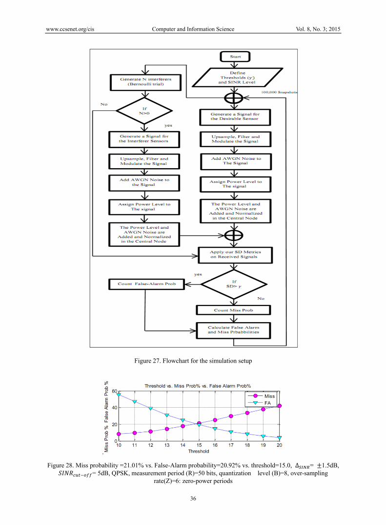
We typically generate 100,000 simulation snapshots where each snapshot generates a random number of interferers up to 30 sensors with random power assignments. Figure 27 shows a flowchart for our simulation setup and procedure.
Figures 28, 29 and 30 show the Miss (purple points) and False-Alarm (cyan points) probabilities versus the choice of the technique comparison threshold level (i.e., above which we decide the packet is valid (collision-free) and vice-versa) for the zero-power periods, the single pilot period, and the double pilot periods techniques respectively, and for QPSK, 8PSK and 16PSK modulation schemes (The choice of system parameters is defined in the caption of the corresponding figure). As shown in the figures, the intersection point of the purple and cyan curves, can be a reasonable point to choose the threshold level in order to have a reasonable (or balanced) consideration of the Miss and False-Alarm probabilities, but certainly a designer can refer to Appendix A to choose an arbitrarily different point for a different criterion of choice.
25 30 35 40 45 50 55 60 65 70 75 8010
0
101
102
Threshold vs. False-Alarm Prob "Simulation and Math Comparison"
Threshold
Fal
se-A
larm
Pro
b %
FA:Simulation
FA:Mathematical
www.ccsenet.org/cis Computer and Information Science Vol. 8, No. 3; 2015
36
Figure 27. Flowchart for the simulation setup
.
Figure 28. Miss probability =21.01% vs. False-Alarm probability=20.92% vs. threshold=15.0, ∆ = ±1.5dB, = 5dB, QPSK, measurement period (R)=50 bits, quantization level (B)=8, over-sampling
rate(Z)=6: zero-power periods

www.ccsenet.org/cis Computer and Information Science Vol. 8, No. 3; 2015
37
Figure 29. Miss probability =6.98% vs. False-Alarm probability=6.95% vs. threshold=79.0, ∆ = ±1dB, = 5dB, QPSK, measurement period= 500 bits, ⁄ = 50%, ℵ= 70%: single-pilot period
Figure 30. Miss probability = 8.25% vs. False Alarm probability=8.25% vs. threshold=40.0, ∆ = ±1dB, = 5dB, 8PSK, measurement period= 1000 bits, = =14 samples, ⁄ = ⁄ = 40%, ℵ =ℵ = 60%: double-pilot periods
Figure 31. Miss probability =36.82% vs. False-Alarm probability=37.02% vs. threshold=15.0, ∆ = ±1dB, = 10dB, 8PSK, measurement period (R)=50 bits, quantization level (B)=4, over-sampling
rate(Z)=2: zero-power periods
Figure 32. Miss probability = 9.88% vs. False Alarm probability=9.96% vs. threshold=46.0, ∆ = ±1.5dB, = 7dB, 16PSK, measurement period= 500 bits, = =16 samples, ⁄ = ⁄ = 50%, ℵ =ℵ = 60%: double-pilot periods

www.ccsenet.org/cis Computer and Information Science Vol. 8, No. 3; 2015
38
8. Conclusion
In this paper we propose novel simple power-efficient low-latency collision detection techniques for WSNs and analyze its performance. We propose three simple statistical discrimination techniques which are applied directly at the receiver’s IQ ADC output to determine if the received signal represents a valid collision-free packet. Hence, saving a significant amount of processing power and collision detection processing time delay, compared to conventional full-decoding mechanisms, which also requires going through the entire complex receiver and modem processing. We also analyze and demonstrate the amount of power saving achieved by our SD approaches compared to the conventional full-decoding approaches. As demonstrated by the numerical results and performance analysis, our novel approaches offer much lower computational complexity (in term of the number of operations per bit) and shorter measurement period compared to full-decoding approaches. The SD approaches allow a system designer multiple degrees of freedom for design trade-offs and optimization through various design parameters.
Despite these encouraging results, we need to perform more experiments to understand the impact of our design techniques when the network has some mobile nodes spread over an infinite area in the presence of Rayleigh fading. For example, we will apply our design techniques in specific applications such as vehicle to vehicle communications.
Acknowledgments
This work has been partially sponsored by Stevens Institute of Technology, Hoboken, NJ, USA and the Taif University of the Kingdom of Saudi Arabia.
References
Kori, R. H., Angadi, A. S., Hiremath, M. K., & Iddalagi, S. M. (2009). Efficient Power Utilization of Wireless Sensor Networks: A Survey. Advances in Recent Technologies in Communication and Computing Conference, ARTCom '09. International Conference on , 571(575), 27-28
Jamieson, K., Balakrishnan, H., & Tay, Y. C. (2003). Sift: A MAC Protocol for Event-Driven Wireless Sensor Networks. MIT Laboratory for Computer Science, Tech. Rep.894
Zorzi, M., & Rao, R. R. (2004). Coding tradeoffs for reduced energy consumption in sensor networks. Personal, Indoor and Mobile Radio Communications, PIMRC 2004. 15th IEEE International Symposium on, 1, 206-210.
Harry, L., & Trees, V. (1968). Detection, Estimation, and Modulation Theory: Part I: John Wiley and Sons.
Chen, J., & Abedi, A. (2011). Distributed Turbo Coding and Decoding for Wireless Sensor Networks. Communications Letters, IEEE, 15(2), 166-168.
Chanchal, K. D., & Sumit, K. (2012). Hybrid Forwarding for General Cooperative Wireless Relaying in m-Nakagami Fading Channel. International Journal of Future Generation Communication and Networking, 5(1).
Hua, G. G., & Chen, C. W. (2005). Distributed source coding in wireless sensor networks. Quality of Service in Heterogeneous Wired/Wireless Networks. Second International Conference on, 7(6), 24-24.
Robertson, P., Villebrun, E., & Hoeher, P. (1995). A comparison of optimal and sub-optimal MAP decoding algorithms operating in the log domain. ICC '95 Seattle, 'Gateway to Globalization. IEEE International Conference on , 2, 18-22.
Cam, H. (2006). Multiple-Input Turbo Code for Joint Data Aggregation,Source and Channel Coding in Wireless Sensor Networks. ICC'06. IEEE International Conference on, 8, 3530-3535
Dam, T. V., & Langendoen, K. (2003). An Adaptive Energy-Efficient MAC Protocol for Wireless Sensor Network. The First ACM Conference on Embedded Networked Sensor Systems (Sensys‘03), Los Angeles, CA, USA
Peng, J., Cheng, L., & Sikdar, B. (2007). A Wireless MAC Protocol with Collision Detection. Mobile Computing, IEEE Transactions on , 6(12), 1357-1369
Tobagi, F. A., & Kleinrock, L. (1975). Packet switching in radio channels: Part II - the hidden terminal problem in carrier sense multiple access and the busy tone solution. IEEE Transactions on Communications, 23, 1417–1433
Akyildiz, I. F. et al. (2002). Wireless sensor networks: a survey. Computer Networks, 38, 393-422.
Lu, G., Krishnamachari, B., & Raghavendra, C. S. (2004). An adaptive energy efficient and low-latency MAC for

www.ccsenet.org/cis Computer and Information Science Vol. 8, No. 3; 2015
39
data gathering in wireless sensor networks. Proceedings of 18th International Parallel and Distributed Processing Symposium, 224, 26-30.
Lin, P., Qiao, C., & Wang, X. (2004). Medium access control with a dynamic duty cycle for sensor networks. IEEE Wireless Communications and Networking Conference, 3, 21-25.
Sandra, S., Jaime, L., Miguel, G., & Jose, F. T. (2011). Power Saving and Energy Optimization Techniques for Wireless Sensor Networks (Invited Paper). Journal of Communications, 6(6), 439-459.
Sungoh, K., & Shroff, N. B. (2006). "Energy-Efficient Interference-Based Routing for Multi-Hop Wireless Networks. INFOCOM 2006. 25th IEEE International Conference on Computer Communications., 1-12.
HolandaFilho, R., da S Araújo, H., & Filho, R. H. (2010). WSN Routing: An Geocast Approach for Reducing Consumption Energy. Wireless Communications and Networking Conference (WCNC), 2010 IEEE, 1(6), 18-21.
El-Aaasser, M., & Ashour, M. (2013). Energy aware classification for wireless sensor networks routing. International Conference Advanced Communication Technology (ICACT), 66(71), 27-30.
Cardei, M., Thai, M. T., Li, Y. S., & Wu, W. L. (2005). Energy-efficient target coverage in wireless sensor networks. INFOCOM 2005. 24th Annual Joint Conference of the IEEE Computer and Communications Societies. Proceedings IEEE, 3, 13-17.
Ma, J. C., Lou, W., Wu, Y. W., Li, M., & Chen, G. H. (2009). Energy Efficient TDMA Sleep Scheduling in Wireless Sensor Networks. INFOCOM 2009, IEEE, 19-25.
Ingelrest, F., Simplot-Ryl, D., Stojmenovic, I. (2007).Smaller Connected Dominating Sets in Ad Hoc and Sensor Networks based on Coverage by Two-Hop Neighbors. Communication Systems Software and Middleware. COMSWARE, 1(8), 7-12.
Heinzelman, W. R., Chandrakasan, A., & Balakrishnan, H. (2000). Energy-efficient communication protocol for wireless microsensor networks. System Sciences. Proceedings of the 33rd Annual Hawaii International Conference on , 10(2), 4-7.
Li, N., Hou, J. C., Sha, L. (2005). Design and analysis of an MST-based topology control algorithm. Wireless Communications, IEEE Transactions on , 4(3). 1195-1206.
David, C. L. (2004).Statistics Concepts and Applications for Science: Jones & Bartlett Pub, second edition.
Li, L., Maunder, R. G., Al-Hashimi, B. M., & Hanzo, L. (2013). A Low-Complexity Turbo Decoder Architecture for Energy-Efficient Wireless Sensor Networks. Very Large Scale Integration (VLSI) Systems, IEEE Transactions on, 21(1), 14-22.
Ye, W., Heidemann, J., & Estrin, D. (2004). Medium Access Control With Coordinated Adaptive Sleeping for Wireless Sensor Networks. IEEE/ACM Transactions on Networking, 12(3), 493-506.
Karapistoli, E., Stratogiannis, D. G., Tsiropoulos, G. I., & Pavlidou, F. (2012).MAC protocols for ultra-wideband ad hoc and sensor networking: A survey. Ultra-Modern Telecommunications and Control Systems and Workshops (ICUMT), 2012 4th International Congress on , 834(841), 3-5.
Miranda, J., Gomes, T., Abrishambaf, R., Loureiro, F., Mendes, J., Cabral, J., & Monteiro, J. L. (2014). A Wireless Sensor Network for collision detection on guardrails. Industrial Electronics (ISIE), 2014 IEEE 23rd International Symposium on , 1430-1435.
Peng, J. et al. (2007). A Wireless MAC Protocol with Collision Detection. IEEE Transactions on Mobile Computing, 6(12).
Y. Shang (2014). Vulnerability of networks: Fractional percolation on random graphs, Physical Review E, 89, 012813.
Appendix
Tables for Simulation Results
In this appendix, we provide more detailed performance results for our proposed techniques for various probability of transmissions per sensor ( ) such as 0.4, 0.3 and 0.2, and for QPSK, 8PSK and 16PSK modulation schemes.We assume = 5dB. In addition, for the single pilot period and the double pilot periods techniques we assume the number of samples per slot ( ) is 2 samples. The simulation parameters are demonstrated in table 2.

www.ccsenet.org/cis Computer and Information Science Vol. 8, No. 3; 2015
40
Table 2. Simulation parameters
Simulation Parameter
Description
R The measurement period in bits
B The number of quantization levels for the received signal envelop
Z The oversampling rate
G The number of slots per pilot period
L The length of the pilot period in single pilot period technique. L = L = L for the double pilot periods technique.
The ratio of zeros slots to ones slots in single pilot period
technique. ,, = ,, = for double pilot periods technique.
V The number of samples per measurement period (i.e. Z×+L; is the number of information bits which are
to one symbol, e.g., M=3 for 8PSK modulation scheme) ℵ The soft decision percentage when decoding the received pilot sequence at the central node in single pilot period technique. ℵ = ℵ = ℵ for double pilot periods technique. ∆ The tolerance level for the SINR (e.g. ∆ = ±1dB means the SINR = 6dB for calculating False-Alarm probabilities and the SINR = 3dB for calculating Miss probabilities when the
is 5 dB). The probability of False-Alarm.
The probability of Miss.
The threshold level (in section IV we explained how to select the threshold level).
Table 3. QPSK, Zero-Power periods scheme, = 0.3.
V ∆ Z B R
56 11.0039.77%39.72%±1dB 2 4 50
156 15.0026.08%26.16%±1dB 6 8 50
206 16.0024.53%24.57%±1dB 8 10 50
56 10.0036.16%36.14%±1.5dB2 4 50
156 15.0021.01%20.92%±1.5dB6 8 50
206 16.0019.12%19.04%±1.5dB8 10 50
110 15.0026.53%26.50%±1dB 2 4 100
310 17.0020.17%20.21%±1dB 6 8 100
410 17.0018.32%18.30%±1dB 8 10 100

www.ccsenet.org/cis Computer and Information Science Vol. 8, No. 3; 2015
41
110 15.0021.02%21.08%±1.5dB2 4 100
310 17.0014.90%14.90%±1.5dB6 8 100
410 17.0012.22%12.20%±1.5dB8 10 100
220 17.0020.01%20.00%±1dB 2 4 200
620 18.0015.84%15.83%±1dB 6 8 200
820 19.0014.06%14.08%±1dB 8 10 200
220 17.0015.00%15.00%±1.5dB2 4 200
620 18.0010.22%10.18%±1.5dB6 8 200
820 18.009.99% 9.90% ±1.5dB8 10 200
550 19.0014.11%14.10%±1dB 2 4 500
1550 19.0011.16%11.10%±1dB 6 8 500
2050 19.0010.15%10.10%±1dB 8 10 500
550 18.0012.19%12.11%±1.5dB2 4 500
1550 18.0010.20%10.15%±1.5dB6 8 500
2050 18.009.22% 9.20% ±1.5dB8 10 500
1100 20.0010.02%10.05%±1dB 2 4 1000
3100 20.008.30% 8.36% ±1dB 6 8 1000
4100 20.007.60% 7.56% ±1dB 8 10 1000
1100 19.009.26% 9.21% ±1.5dB2 4 1000
3100 19.007.41% 7.43% ±1.5dB6 8 1000
4100 19.006.18% 6.20% ±1.5dB8 10 1000
Table 4. 8PSK, Zero-Power periods scheme, = 0.3.
V ∆ ZBR
38 6.0044.45%43.76%±1dB 2 4 50
10213.003819%38.11%±1dB 6 8 50
13415.0028.40%28.44%±1dB 8 10 50
38 6.0038.06%38.04%±1.5dB2 4 50
10213.0029.61%29.60%±1.5dB6 8 50
13414.0026.33%26.32%±1.5dB8 10 50
74 13.0031.10%31.13%±1dB 2 4 100
20217.0023.34%23.33%±1dB 6 8 100
26617.0019.20%19.25%±1dB 8 10 100

www.ccsenet.org/cis Computer and Information Science Vol. 8, No. 3; 2015
42
74 13.0025.10%25.11%±1.5dB2 4 100
20216.0019.10%19.13%±1.5dB6 8 100
26616.0017.13%17.12%±1.5dB8 10 100
15216.0023.12%23.15%±1dB 2 4 200
41618.0016.60%16.65%±1dB 6 8 200
64718.0015.17%15.14%±1dB 8 10 200
15215.0019.00%19.03%±1.5dB2 4 200
41618.0011.92%11.94%±1.5dB6 8 200
64717.0010.24%10.20%±1.5dB8 10 200
38218.0018.40%18.40%±1dB 2 4 500
1046 18.0013.10%13.20%±1dB 6 8 500
1378 18.0017.33%17.32%±1dB 8 10 500
38218.0013.09%13.01%±1.5dB2 4 500
1046 18.0011.00%11.03%±1.5dB6 8 500
1378 17.0010.11%10.11%±1.5dB8 10 500
76618.0013.12%13.12%±1dB 2 4 1000
2098 19.0010.02%10.01%±1dB 6 8 1000
2764 20.008.21%8.22% ±1dB 8 10 1000
76620.0010.24%10.21%±1.5dB2 4 1000
2098 20.008.12%8.11%±1.5dB6 8 1000
2764 20.007.65%7.64%±1.5dB8 10 1000
Table 5. 16PSK, Zero-Power periods scheme, α=0.3.
V ∆ ZBR
30 6.0046.21%46.22%±1dB 2 4 50
78 12.0039.33%39.21%±1dB 6 8 50
10213.0033.77%33.76%±1dB 8 10 50
30 6.0039.13%39.11%±1.5dB2 4 50
78 11.0032.10%32.12%±1.5dB6 8 50
10213.0029.51%29.54%±1.5dB8 10 50
60 11.0033.30%33.23%±1dB 2 4 100
16015.0025.22%25.21%±1dB 6 8 100
21016.0022.32%22.32%±1dB 8 10 100
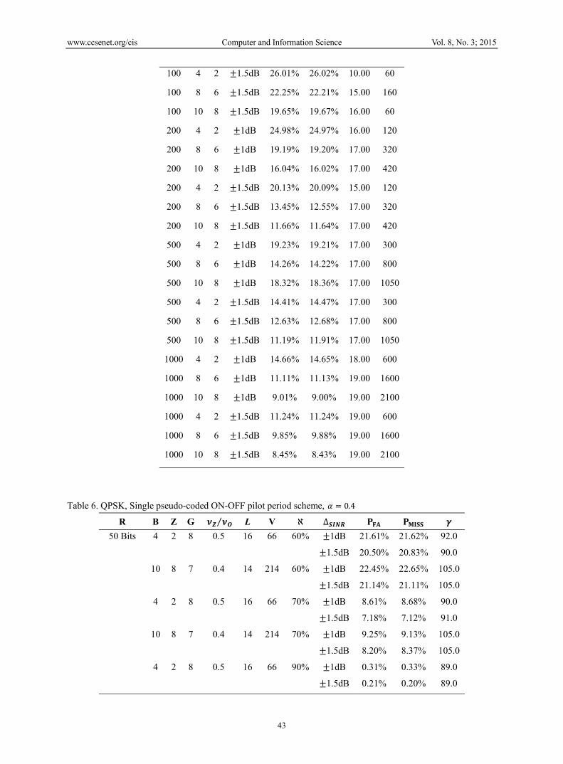
www.ccsenet.org/cis Computer and Information Science Vol. 8, No. 3; 2015
43
60 10.0026.02%26.01%±1.5dB2 4 100
16015.0022.21%22.25%±1.5dB6 8 100
60 16.0019.67%19.65%±1.5dB8 10 100
12016.0024.97%24.98%±1dB 2 4 200
32017.0019.20%19.19%±1dB 6 8 200
42017.0016.02%16.04%±1dB 8 10 200
12015.0020.09%20.13%±1.5dB2 4 200
32017.0012.55%13.45%±1.5dB6 8 200
42017.0011.64%11.66%±1.5dB8 10 200
30017.0019.21%19.23%±1dB 2 4 500
80017.0014.22%14.26%±1dB 6 8 500
1050 17.0018.36%18.32%±1dB 8 10 500
30017.0014.47%14.41%±1.5dB2 4 500
80017.0012.68%12.63%±1.5dB6 8 500
1050 17.0011.91%11.19%±1.5dB8 10 500
60018.0014.65%14.66%±1dB 2 4 1000
1600 19.0011.13%11.11%±1dB 6 8 1000
2100 19.009.00%9.01% ±1dB 8 10 1000
60019.0011.24%11.24%±1.5dB2 4 1000
1600 19.009.88% 9.85%±1.5dB6 8 1000
2100 19.008.43%8.45%±1.5dB8 10 1000
Table 6. QPSK, Single pseudo-coded ON-OFF pilot period scheme, = 0.4
∆ℵ V L ⁄ GZ BR
92.021.62%21.61%±1dB 60%66 160.5 824 50 Bits .09020.83%20.50%±1.5dB
105.022.65%22.45% ±1dB 60%214140.4 7810
.0105 21.11% 21.14%±1.5dB
90.08.68% 8.61% ±1dB 70%66 160.5 824
.0917.12% 7.18%±1.5dB
105.09.13%9.25%±1dB 70%214140.4 7810
.01058.37%8.20%±1.5dB
89.0 0.33%0.31% ±1dB 90%66 160.5 824
.089 0.20%0.21%±1.5dB
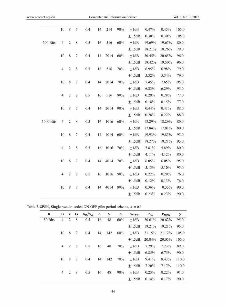
www.ccsenet.org/cis Computer and Information Science Vol. 8, No. 3; 2015
44
105.00.45%0.47%±1dB 90%214 140.4 7810
105.00.30%0.30%±1.5dB
80.019.65% 19.69% ±1dB 60% 516160.5 824 500 Bits 79.018.26%18.21%±1.5dB
96.020.65%20.45%±1dB 60%2014 140.4 7810
96.019.50% 19.42%±1.5dB
79.0 6.98%6.95%±1dB 70%516160.5 824
79.05.34%5.32%±1.5dB
95.07.65%7.45%±1dB 70%2014140.4 7810
95.0 6.29%6.23%±1.5dB
77.00.28%0.29%±1dB 90%516160.5 824
.0770.15%0.18% ±1.5dB
88.00.41%0.44% ±1dB 90%2014140.4 7810
88.00.22%0.28%±1.5dB
80.018.29%18.29%±1dB 60%1016160.5 824 1000 Bits .08017.81%17.84%±1.5dB
95.019.85%19.93%±1dB 60%4014140.4 7810
95.018.21%18.27%±1.5dB
80.05.89% 5.81%±1dB 70%1016160.5 824
.080 4.12%4.11%±1.5dB
95.06.05% 6.05%±1dB 70%4014140.4 7810
95.05.10%5.13%±1.5dB
76.00.20%0.22%±1dB 90%101616 0.5 824
76.00.13% 0.12%±1.5dB
90.00.35% 0.36%±1dB 90%4014140.4 7810
90.00.23%0.23%±1.5dB
Table 7. 8PSK, Single pseudo-coded ON-OFF pilot period scheme, = 0.3
∆ℵ V L ⁄ GZ BR
95.020.62%20.61%±1dB 60%48 160.5 824 50 Bits .09519.21%19.21%±1.5dB
105.021.12%21.15% ±1dB 60%142 140.4 7810
.0105 20.05% 20.04%±1.5dB
89.07.23% 7.29% ±1dB 70%48 160.5 82 4
.0906.75% 6.85%±1.5dB
110.08.43%9.41%±1dB 70%142140.4 7810
.01107.17%7.20%±1.5dB
91.0 0.22%0.23% ±1dB 90% 48 160.5 824
.090 0.17%0.14%±1.5dB

www.ccsenet.org/cis Computer and Information Science Vol. 8, No. 3; 2015
45
104.00.32%0.37%±1dB 90%142 140.4 7810
104.00.23%0.21%±1.5dB
80.018.15% 18.19% ±1dB 60% 348160.5 824 500 Bits 79.017.20%17.13%±1.5dB
99.018.95%18.97%±1dB 60%1342 140.4 7810
98.017.10% 17.12%±1.5dB
80.0 6.01%6.05%±1dB 70%348160.5 824
80.05.14% 5.12%±1.5dB
99.06.97%6.95%±1dB 70%1342140.4 7810
99.0 5.50%5.43%±1.5dB
77.00.20%0.19%±1dB 90%348160.5 824
.0770.13%0.14% ±1.5dB
90.00.35%034% ±1dB 90%1342140.4 7810
90.00.19%0.18%±1.5dB
80.0 17.91%17.98%±1dB 60%682160.5 824 1000 Bits .08016.31%16.34%±1.5dB
99.017.15%17.13%±1dB 60%2678140.4 7810
98.016.51%16.56%±1.5dB
80.05.09% 5.01%±1dB 70% 682160.5 824
.080 4.02%4.01%±1.5dB
99.05.85% 5.95%±1dB 70% 2678140.4 7810
99.04.50%4.53%±1.5dB
76.00.19%0.20%±1dB 90%682 16 0.5 824
76.00.09% 0.08%±1.5dB
98.00.28% 0.26%±1dB 90%2678140.4 7810
98.00.13%0.14%±1.5dB
Table 8. 16PSK, Single pseudo-coded ON-OFF pilot period scheme, = 0.2
∆ℵ V L ⁄ GZ BR
96.019.17%19.11%±1dB 60%40 160.5 82 4 50 Bits 6.09 18.73%18.77%±1.5dB
106.0 20.13%20.16% ±1dB 60%110140.4 7810
.0106 19.15% 19.14%±1.5dB
92.06.63% 6.69% ±1dB 70%40 160.5 82 4
.0925.79% 5.86%±1.5dB
113.07.73%7.71%±1dB 70%110140.4 7810
.01136.03%6.09%±1.5dB
92.0 0.16%0.17% ±1dB 90% 40 160.5 824
.092 0.08%0.06%±1.5dB
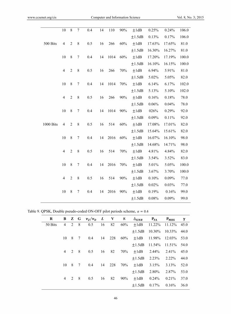
www.ccsenet.org/cis Computer and Information Science Vol. 8, No. 3; 2015
46
106.00.24%0.25%±1dB 90%110 140.4 7810
106.00.17%0.13%±1.5dB
81.017.65% 17.63% ±1dB 60% 266160.5 824 500 Bits 81.016.27%16.30%±1.5dB
100.017.19%17.20%±1dB 60%1014 140.4 7810
100.016.15% 16.10%±1.5dB
81.0 5.91%6.94%±1dB 70%266160.5 824
82.05.05% 5.02%±1.5dB
102.06.17%6.14%±1dB 70%1014140.4 7810
102.0 5.10%5.13%±1.5dB
78.00.18%0.16%±1dB 90%266160.5 824
.0780.04%0.06% ±1.5dB
92.00.29%026% ±1dB 90%1014 140.4 7810
92.00.11%0.09%±1.5dB
82.0 17.01%17.08%±1dB 60%514160.5 824 1000 Bits .08215.61%15.64%±1.5dB
98.016.10%16.07%±1dB 60%2016140.4 7810
98.014.71%14.68%±1.5dB
82.04.84% 4.81%±1dB 70% 514160.5 824
.083 3.52%3.54%±1.5dB
100.05.05% 5.01%±1dB 70% 2016140.4 7810
100.0 3.70%3.67%±1.5dB
77.00.09%0.10%±1dB 90%51416 0.5 824
77.00.03% 0.02%±1.5dB
99.00.16% 0.19%±1dB 90%2016 140.4 7810
99.00.09%0.08%±1.5dB
Table 9. QPSK, Double pseudo-coded ON-OFF pilot periods scheme, = 0.4
∆ℵ V L ⁄GZBR
45.011.12%11.22%±1dB 60%82 160.5 82450 Bits
.04410.33%10.30%±1.5dB
53.012.03%11.98%±1dB 60%228140.4 7810
.05411.51%11.54%±1.5dB
45.02.41%2.44%±1dB 70%82 160.5 824
.0442.22%2.23%±1.5dB
52.03.13%3.15%±1dB 70%228140.4 7810
.0532.87%2.80%±1.5dB
37.00.21%0.24%±1dB 90%82 160.5 824
.036 0.16%0.17%±1.5dB

www.ccsenet.org/cis Computer and Information Science Vol. 8, No. 3; 2015
47
48.00.15%0.14%±1dB 90%228140.4 7810
50.00.09%0.09%±1.5dB
40.010.20%10.12%±1dB 60%532160.5 824500 Bits
40.09.91%9.94%±1.5dB
54.011.45%11.44%±1dB 60%2028140.4 7810
54.010.20%10.22%±1.5dB
39.0 2.25% 2.25% ±1dB 70%532160.5 824
39.0 2.04%2.02%±1.5dB
49.03.02% 3.04%±1dB 70%2028140.4 7810
49.02.39%2.33%±1.5dB
37.00.10%0.10%±1dB 90%532160.5 824
.0390.05%0.04%±1.5dB
48.00.13%0.12%±1dB 90%2028140.4 7810
48.00.08%0.08%±1.5dB
39.09.95%9.90%±1dB 60%1032160.5 8241000 Bits
.0398.71%8.77%±1.5dB
40.010.15%10.13%±1dB 60%4028140.4 7810
40.09.11%9.17%±1.5dB
39.02.02%2.01%±1dB 70%1032160.5 824
.0391.84%1.87% ±1.5dB
50.01.75%1.77%±1dB 70%4028140.4 7810
50.01.01%1.03%±1.5dB
36.00.06%0.07%±1dB 90%1032160.5 824
40.00.01%0.01% ±1.5dB
48.00.08%0.08%±1dB 90% 4028140.4 7810
48.00.02%0.03%±1.5dB
Table 10. 8PSK, Double pseudo-coded ON-OFF pilot periods scheme, = 0.3
∆ℵ V L⁄GZBR
48.010.31%10.32%±1dB60%64 160.5 82450 Bits
.0489.13%9.13%±1.5dB
59.011.33%11.38%±1dB60%156140.4 7810
.05910.11%10.12%±1.5dB
47.0 1.91%1.92%±1dB70%64 160.5 824
.0481.31%1.32%±1.5dB
58.03.01%3.05%±1dB70%156140.4 7810
.0582.51%2.50%±1.5dB
43.00.16% 0.15%±1dB90%64 160.5 824
.043 0.10%0.09%±1.5dB
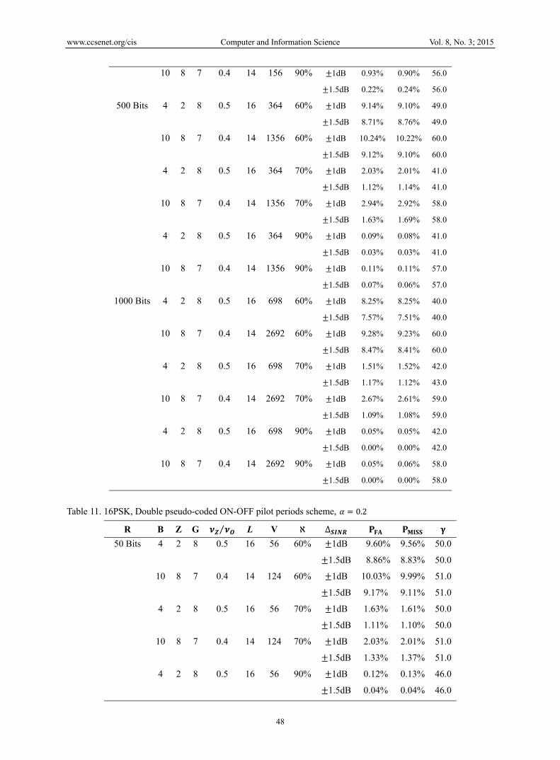
www.ccsenet.org/cis Computer and Information Science Vol. 8, No. 3; 2015
48
56.00.90%0.93% ±1dB90%156140.4 7810
56.00.24%0.22%±1.5dB
49.09.10%9.14%±1dB60%364160.5 824500 Bits
49.08.76%8.71%±1.5dB
60.010.22%10.24%±1dB60%1356140.4 7810
60.09.10%9.12%±1.5dB
41.0 2.01% 2.03% ±1dB 70%364160.5 824
41.0 1.14%1.12%±1.5dB
58.0 2.92% 2.94%±1dB70%1356140.4 7810
58.01.69%1.63%±1.5dB
41.00.08%0.09% ±1dB90%364160.5 824
.0410.03%0.03%±1.5dB
57.00.11%0.11%±1dB90%1356140.4 7810
57.00.06%0.07%±1.5dB
40.08.25% 8.25%±1dB60%698160.5 8241000 Bits
40.07.51%7.57%±1.5dB
60.09.23%9.28%±1dB60%2692140.4 7810
60.08.41%8.47%±1.5dB
42.01.52%1.51%±1dB70%698160.5 824
.0431.12%1.17% ±1.5dB
59.02.61%2.67%±1dB70%2692140.4 7810
59.01.08%1.09%±1.5dB
42.00.05%0.05%±1dB 90%698160.5 824
42.00.00%0.00% ±1.5dB
58.00.06%0.05%±1dB90%2692140.4 7810
58.00.00%0.00%±1.5dB
Table 11. 16PSK, Double pseudo-coded ON-OFF pilot periods scheme, = 0.2
∆ℵ V L⁄GZBR
50.09.56%9.60% ±1dB 60%56 160.5 82450 Bits
.0508.83%8.86% ±1.5dB
51.09.99%10.03%±1dB 60%124140.4 7810
51.0 9.11%9.17%±1.5dB
50.0 1.61%1.63%±1dB 70%56 160.5 824
.0501.10%1.11%±1.5dB
51.02.01%2.03%±1dB 70%124140.4 7810
.0511.37% 1.33%±1.5dB
46.00.13% 0.12%±1dB 90%56 160.5 824
.046 0.04%0.04%±1.5dB

www.ccsenet.org/cis Computer and Information Science Vol. 8, No. 3; 2015
49
49.00.60%0.63%±1dB 90%124140.4 7810
49.00.09%0.08%±1.5dB
40.0 8.53% 8.54%±1dB 60%282160.5 824500 Bits
40.07.86%7.84%±1.5dB
41.09.33%9.32%±1dB 60%1028140.4 7810
41.08.91%9.92%±1.5dB
40.0 1.98% 1.98% ±1dB 70%282160.5 824
40.0 1.10%1.09%±1.5dB
40.0 2.22% 2.22%±1dB 70%1028140.4 7810
40.01.18%1.12%±1.5dB
39.00.07%0.07% ±1dB 90%282160.5 824
.0390.00%0.00%±1.5dB
40.00.10%0.10%±1dB 90%1028140.4 7810
40.00.02%0.03%±1.5dB
39.07.85% 7.84%±1dB 60%530160.5 8241000 Bits
39.06.82%6.87%±1.5dB
40.09.03%9.01%±1dB 60%2030140.4 7810
40.08.20%8.16%±1.5dB
39.01.41%1.40%±1dB 70%530160.5 824
.0391.08%1.07% ±1.5dB
40.02.01%2.07%±1dB 70%2030140.4 7810
40.00.07%0.08%±1.5dB
38.00.03%0.03%±1dB 90%530160.5 824
38.00.00%0.00% ±1.5dB
39.00.05%0.04%±1dB 90%2030140.4 7810
39.00.00%0.00%±1.5dB
Notes
Note 1 In this paper, we shall refer to our proposed approach as the “Statistical Discriminator, or SD” method. We shall also refer to the traditional full-decoding methods as “FD” methods.
Note 2 We assume the maximum number of sensors i.e. W= 30. This number can be tuned as required is order to
meet designers' requirements.
Note 3 We assume the length of the zero-power period ( ) is 5% of the total number of samples. In our design we try to minimize as much as possible without degradation in the system performance. However, a designer may select = 3% or 4%.
Note 4 In order to have a threshold setting that is independent of the absolute level of the received signal power
(hence independent of path loss, receiver gain …etc.) the collected IQ samples of the measurement period may
first be normalized to unity power.
Note 5 For Maximum Likelihood Estimation (MLE), see for example, (Trees,1968)
Note 6 Our system throughput is defined as Throughput =(1− ); Where denotes the False-Alarm probability.

www.ccsenet.org/cis Computer and Information Science Vol. 8, No. 3; 2015
50
Note 7 Similar assumptions were made in (Robertson, Villebrun and Hoeher,1995).
Note 8 In this example we assume the single pseudo-coded ON-OFF pilot period technique is used.
Note 9 We simulate 100,000~1,000,000 snapshots per case.
Note 10 We simulate the random path-loss effect by simply generating random received power levels from the
various sensors at the access node.
Note 11 In our analysis, we limit the maximum number of sensors in a simulation snapshot to 30 sensors.
Note 12 A 5dB SINR seems a reasonable assumption based on typical coding requirements in wireless systems
(Dey and Kundu,2012).
Copyrights
Copyright for this article is retained by the author(s), with first publication rights granted to the journal.
This is an open-access article distributed under the terms and conditions of the Creative Commons Attribution license (http://creativecommons.org/licenses/by/3.0/).


![[1913] #2.12 Armour's Monthly Cook Book - October 1913](https://static.fdocuments.in/doc/165x107/577d2da61a28ab4e1eae0102/1913-212-armours-monthly-cook-book-october-1913.jpg)


