Models of simple animal tissues

Author: Meta Kokalj

Advisor: doc. dr. Primož Ziherl

Ljubljana, February 2011

Summary

Animals are biological entities but their structure and dynamics depends on the mechanical

properties of eukaryotic cells as their basic units and on cell-cell interactions. In this seminar, the

basic physical models of simple cell aggregates are presented. We review the microscopic origin of

the main physical mechanisms and forces in question, and we present selected examples of cell

aggregates and structures that can be described in terms of physical model.

2

Table of contents:

1. Introduction ....................................................................................................................................2

1.1. Why are animal tissue models useful? ......................................................................................2

1.2. Biological point of view.............................................................................................................2

1.3. Physical point of view ...............................................................................................................3

2. Minimal energy models ...................................................................................................................4

2.1. Small cell agregates..................................................................................................................5

2.2. Bulk cell aggregate ...................................................................................................................7

2.3. Anisotropy ................................................................................................................................9

2.4. Tissue surface tension ............................................................................................................. 10

2.5. Differential adhesion hypotheses ............................................................................................ 11

3. Kinetic models .............................................................................................................................. 13

4. Conclusion .................................................................................................................................... 15

References ........................................................................................................................................ 15

1. Introduction

1.1. Why are animal tissue models useful?

Understanding the tissue formation and cell migration is very important. This knowledge could be applied to in vitro and in vivo systems to improve their functionality. The in vitro systems can be used to produce a chemical compound, which is then used for example as a medicine (antibiotics). This kind of systems can also be used for tissue growth for transplantation. In the first case, the knowledge about cell shape and tissue formation is important because sometimes the desired compound is synthesized only under specific conditions which may involve cell-cell adhesion. By understanding what triggers this adhesion one could control the synthesis by adding the stimulants for the desired process. The in vitro growth of organs and tissues for transplantation is an even more complex process to control and the understanding of how the cell shape and cell packing affect it one could improve its applicability. More optimistic and complex application is in vivo, in the living organisms. The medicines for the diseases that are caused by irregularities in growth and formation of organs could be developed [1].

1.2. Biological point of view

By exploring the tissue formation one must first understand the basic unit of the system, which is the cell. For better understanding it is important to know the cell from different points of view. Let us summarize the biologist’s point of view (Figure 1a). The cell is surrounded by a cell membrane (Figure 1b). The base of a cell membrane is a lipid bilayer in which many proteins are embedded. These proteins play many different roles. Some of those proteins are connected to the intracellular matrix. Others enable adhesion of the cell to other cells. This can be mediated by tight junctions (the membranes of neighboring cells are fused, thus forming a continuous belt) (Figure 1c), desmosomes (junctions mediated by protein molecules that are also attached to the intracellular matrix

3

constituted from actin and miosin) (Figure 1d) and gap junctions (cytoplasmic channels, point junctions mediated by transmembrane proteins of both cells) (Figure 1e). In this seminar adherens junctions will often be discussed. These are a type of desmosome cell-cell junctures that are mediated by cadherin molecules and are located as a thin belt. The main elements of the the biological image of a cell are the lipid bilayer, the proteins that allow adhesion to neighboring cells, and the inner matrix that has its own elastic and contractile properties [2].

Figure 1: (a) Animal cell and its basic organelles [3], (b) the cell membrane and its components [4]. Different types of cell-cell junctions: (c) tight junction [2], (d) desmosome [2], (e) gap junction [2].

1.3. Physical point of view

Experimentally, the full 3D shape of cells is not easily accessible. Most studies are restricted to layered (or even single-layer) tissues where cells are assumed to have a prismatic shape of fixed height (Figure 2). In this case, each cell is represented by its cross-section area instead of the volume and a 2D surface which is the perimeter.

Figure 2: Prismatic cells. (a) an aggregate of prismatic cells, (b) prismatic cell with cross-section area A and perimeter P [5].

Let us assume that the shape of cells in an aggregate corresponds to a minimum of an energy functional and let us try to understand the main phenomenological terms in this functional.

Firstly, cell volume is known not to vary too much. When looking at the cross-section of cells in fairly monodisperse tissues, the area variation is typically restricted to about 10 % [6]. So it is reasonable to assume that there must be a term that penalizes any deviation from a preferred cross-section area, and the simplest form is

, (1)

where A0i is the preferred cross-section cell area and is the area modulus; is the actual cell cross-section.

4

Surface energy

Cell shape and form in tissues are shaped by mechanisms following physical principles. One of the possible approaches is that cells organize themselves within structures that minimize their total surface area [7]. The 2D surface energy is

, (2)

where is linear energy density (surface tension in 2D) which is always positive and is the

2D surface area which is the perimeter [7]. It is well-known that the least perimeter 2D shapes are circles.

Adhesion energy

Cadherin adhesion molecules are the most widespread molecules that mediate adhesion among animal cells, and their role has been demonstrated in cell sorting, migration, tumor invasibility, cell intercalation, packing of epithelial cells, axon outgrowth etc. [7]. A suitable model for cell-cell adhesion is similar to the one for the surface energy except for the sign. The consequence of the surface energy is perimeter minimization, because of the adhesion energy the perimeter spreads and this makes the cell unstable [8]. In the 2D model the adhesion energy reads

, (3)

where is a positive constant depending on the type and density of adhesion molecules and is the total perimeter of cell-cell contacts.

Cortical tension

The actin and myosin form a network under the cell membrane which has elastic properties. This network is contractile and generates tension, this tension depends on the surface area of the cell, the size of which depends on the cell’s shape, which in turn depends on the tension; there is a feedback between tension and shape and thus between each cell and its neighbors [8]. This energy can be modeled by

, (4)

and are the cell perimeter and the cell preferred perimeter. is positive line tension constant that is a consequence of cortical network. is a positive constant which depends on elastic properties of the network. Line tension describes

forces resulting from cell-cell interactions along the junctional regions of specific cell boundaries. Several mechanisms might influence line tension, which could vary from edge to edge. As the cell boundary between two vertices i and j increases, this term in the energy function decreases if the

combined line tension is negative. Conversely, the energy increase with if is positive [9].

2. Minimal energy models

Many cell aggregates resemble clumps of soap bubbles. Thus one could conclude that the cell packing is derived by the surface energy minimization. The soap films between bubbles are always under a positive tension, . This surface tension describes the energy cost of a unit of interface between bubbles and drives their packing. In equilibrium soap bubbles in a 2D foam layer meet by three at each vertex, because four-bubble vertices are unstable. Because is constant and the same for all interfaces, bubble walls meet at equal 120° angles. The 2D foam reaches equilibrium when it minimizes P (the overall perimeter of bubbles), balanced by another constraint fixing each bubble's

5

area [8]. On the other hand there are also important differences between soap bubbles and cell aggregates. In an aggregate of bubbles, interfaces between neighbouring bubbles become single membranes, thus reducing the total surface area and the surface free energy. In an aggregate of cells, adhesion molecules link cell membranes together, contributing to their surface free energy. When the area of adhesion spreads (increasing the cell-cell interface), this surface free energy is reduced [7].

2.1. Small cell agregates

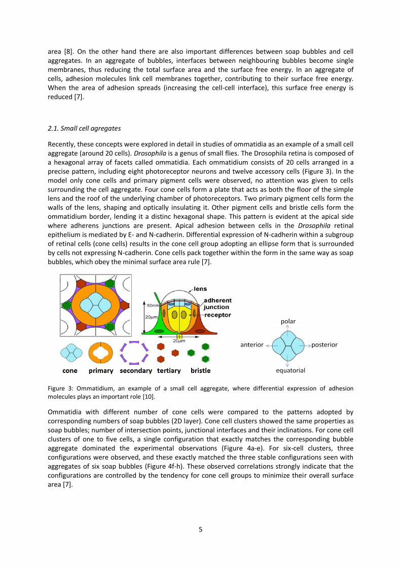
Recently, these concepts were explored in detail in studies of ommatidia as an example of a small cell aggregate (around 20 cells). Drosophila is a genus of small flies. The Drosophila retina is composed of a hexagonal array of facets called ommatidia. Each ommatidium consists of 20 cells arranged in a precise pattern, including eight photoreceptor neurons and twelve accessory cells (Figure 3). In the model only cone cells and primary pigment cells were observed, no attention was given to cells surrounding the cell aggregate. Four cone cells form a plate that acts as both the floor of the simple lens and the roof of the underlying chamber of photoreceptors. Two primary pigment cells form the walls of the lens, shaping and optically insulating it. Other pigment cells and bristle cells form the ommatidium border, lending it a distinc hexagonal shape. This pattern is evident at the apical side where adherens junctions are present. Apical adhesion between cells in the Drosophila retinal epithelium is mediated by E- and N-cadherin. Differential expression of N-cadherin within a subgroup of retinal cells (cone cells) results in the cone cell group adopting an ellipse form that is surrounded by cells not expressing N-cadherin. Cone cells pack together within the form in the same way as soap bubbles, which obey the minimal surface area rule [7].

Figure 3: Ommatidium, an example of a small cell aggregate, where differential expression of adhesion molecules plays an important role [10].

Ommatidia with different number of cone cells were compared to the patterns adopted by corresponding numbers of soap bubbles (2D layer). Cone cell clusters showed the same properties as soap bubbles; number of intersection points, junctional interfaces and their inclinations. For cone cell clusters of one to five cells, a single configuration that exactly matches the corresponding bubble aggregate dominated the experimental observations (Figure 4a-e). For six-cell clusters, three configurations were observed, and these exactly matched the three stable configurations seen with aggregates of six soap bubbles (Figure 4f-h). These observed correlations strongly indicate that the configurations are controlled by the tendency for cone cell groups to minimize their overall surface area [7].

6

Figure 4: Similarity between soap bubbles (leftmost column) and cell aggregates in ommatidia (rightmost column) is obvious [7].

Cells, however, differ greatly from bubbles, in both their membrane and internal composition. Adhesive cells have a tendency to increase their contact interfaces rather than minimize them. In addition cortical cytoskeleton has been shown to determine surface tension to a large extent. Therefore the cell surface tension results from the opposite actions of adhesion and cytoskeletal contraction [8].

Calculating the equilibrium shape of a cluster of more than four bubbles is difficult; for this purpose a numerical method is used to test whether cell patterning is based on surface minimization. In the model proposed in Ref. [8], simulations started from unstable initial conditions designed to favor the random search of final stable topologies. With simulation a local equilibrium was found where the simulated shape no longer changed. This shape was then compared with the experimental results. For each model, parameters that influence the shape of C cells were determined [8].

The assumptions in the model described by Eq. (5) is: (i) adhesion strength is determined by the presence of E- and N-cadherins (when the two of them are present the adhesion is stronger); (ii) to model Roi-mutants only the number of cone cells needs to be changed [8]. The model includes differential adhesion in , a prefered cell area and an elastic cell cortex term,

, where

is the perimeter modulus, and is the preferred perimeter of cell i. The cell perimeter is the sum of its interfaces, . The energy in this model is:

(5)

The interfacial tension between cells i and j is the energy change associated with a

change in membrane length:

(6)

The target perimeter is always smaller than the perimeter; therefore the interfacial tension is

always positive, otherwise the cell would be unstable and fall apart [8].

Wild type

The cells relax either into the correct topology where the polar and equatorial cells touch or into the incorrect one where anterior and posterior cells touch. In the correct topology also the contact angles measured in simulations and experiments agree quite well [8].

Roi mutants

With no additional parameters, simulations with different numbers of C cells were run. For one, two, three, five C cells only one topology is observed in experiments and the same one is observed in simulations (Figure 5a-c). For six cells, three topologies are observed experimentally (Figure 5d-f).

7

Theoretically there are two more possible equilibrium topologies for six cell aggregates, which are never observed. Also with simulation those were the only three topologies found. In two of these cases the entire ommatidium is elongated, to include this in the simulation more free parameters should be added [8].

Figure 5: Experimental and simulation topologies for (a) two, (b) three, (c) five and (d,e,f) six C cells for equation (6) model [8].

In this model, the perimeter modulus λP and the target perimeter P0i reflect the role of the cortical cytoskeleton. The simulated ommatidia and the experimental observations agree very well, therefore it can be concluded that the cytoskeleton play an important role in this cell aggregate[8].

2.2. Bulk cell aggregate

Let us now explore the same mechanical model in an infinite, bulk system, which can be considered a model of single-cell thick tissues such as epithelia. The energy to be minimized includes cell elasticity, and junctional forces arising from cortical contractility and adhesion [9]:

(7)

Line tension describes forces resulting from cell-cell interactions along the junctional regions of

specific cell boundaries. Various mechanisms might influence line tension, which could vary from edge to edge. For example, adhesive interactions between cells could favor cell-boundary expansion, whereas, the subcortical actin skeleton might oppose it. As the cell boundary between cells i and j

increases, this term in the energy function decreases if the line tension is negative and increases if

is positive, depending on which of those two has a bigger effect. Many epithelial cells also have an

actin-myosin belt at the level of apical junctions. Actin-myosin contractility tends to reduce the perimeter of each cell therefore it does not only contribute to the line tension but also generates the

parameter , describing the dependence of contractile tension on cell perimeter [9].

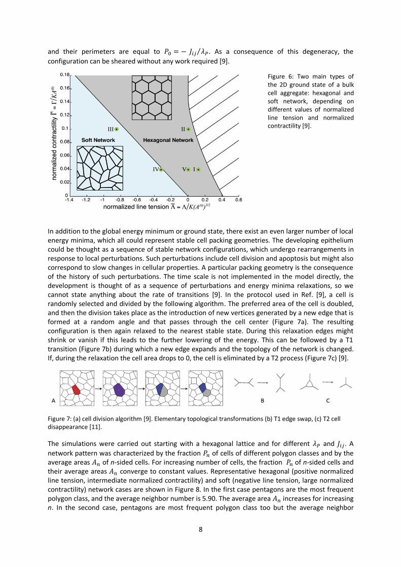
In a tissue of cells of identical and identical two main types of ground state exist as a

function of model parameters. The geometry of the ground state is determined by two normalized parameters; normalized contractility and normalized line tension. When normalized contractility is small, it implies that contractile forces ( are small compared to those of area elasticity ( . Similarly, when normalized line tension is negative, cell boundaries tend to expand; when it is positive, they tend to shrink. Two main types of ground state are hexagonal network and soft network (Figure 6). For the hexagonal type only one ground state exists, this is regular hexagonal packing. This network configuration has both a bulk modulus and a shear modulus; this means that work is required to compress or expand the tissue and also to shear it. For the soft network the ground state is degenerate, there exist many packing geometries all with the same minimal energy. These geometries share a common feature that the area of all cells is equal to the preferred area A0,

8

and their perimeters are equal to . As a consequence of this degeneracy, the

configuration can be sheared without any work required [9].

Figure 6: Two main types of the 2D ground state of a bulk cell aggregate: hexagonal and soft network, depending on different values of normalized line tension and normalized contractility [9].

In addition to the global energy minimum or ground state, there exist an even larger number of local energy minima, which all could represent stable cell packing geometries. The developing epithelium could be thought as a sequence of stable network configurations, which undergo rearrangements in response to local perturbations. Such perturbations include cell division and apoptosis but might also correspond to slow changes in cellular properties. A particular packing geometry is the consequence of the history of such perturbations. The time scale is not implemented in the model directly, the development is thought of as a sequence of perturbations and energy minima relaxations, so we cannot state anything about the rate of transitions [9]. In the protocol used in Ref. [9], a cell is randomly selected and divided by the following algorithm. The preferred area of the cell is doubled, and then the division takes place as the introduction of new vertices generated by a new edge that is formed at a random angle and that passes through the cell center (Figure 7a). The resulting configuration is then again relaxed to the nearest stable state. During this relaxation edges might shrink or vanish if this leads to the further lowering of the energy. This can be followed by a T1 transition (Figure 7b) during which a new edge expands and the topology of the network is changed. If, during the relaxation the cell area drops to 0, the cell is eliminated by a T2 process (Figure 7c) [9].

Figure 7: (a) cell division algorithm [9]. Elementary topological transformations (b) T1 edge swap, (c) T2 cell disappearance [11].

The simulations were carried out starting with a hexagonal lattice and for different and . A

network pattern was characterized by the fraction of cells of different polygon classes and by the average areas of n-sided cells. For increasing number of cells, the fraction of n-sided cells and their average areas converge to constant values. Representative hexagonal (positive normalized line tension, intermediate normalized contractility) and soft (negative line tension, large normalized contractility) network cases are shown in Figure 8. In the first case pentagons are the most frequent polygon class, and the average neighbor number is 5.90. The average area increases for increasing n. In the second case, pentagons are most frequent polygon class too but the average neighbor

9

number is smaller than in the first case, 5.46. All polygons have the same area and the same perimeter . As a consequence, the cell area does not depend on neighbor number.

Results show that for the wing disc tissue best agreement is achieved with parameters that are characteristic for hexagonal network. It is expected that polygon area sizes of soft network do not agree with experiment, since in the model a constant cell area was imposed which is not observed experimentally (Figure 8) [9].

Figure 8: Results for hexagonal and soft network model parameters. Most left column: Stationary network patterns generated by repeated cell division, different colors represent cells with different neighbor number. Middle column: Stationary distribution of neighbor numbers (red bars) and experimental distribution (green). Most right column: Average areas of different polygon glasses for simulation (red line) and experimental (green line). Both networks agree well with experimental data according to the polygon distribution. The size of a certain polygon agrees much better in the hexagonal network [9].

2.3. Anisotropy

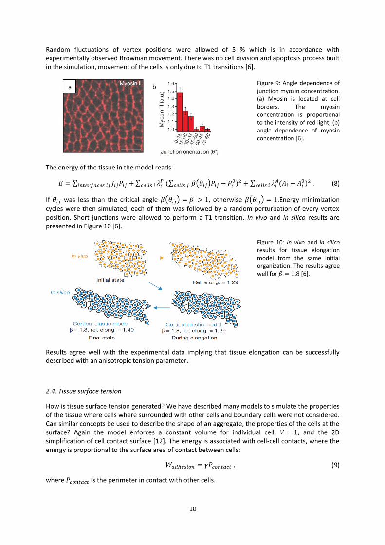
So far only steady states were addressed. What about mechanical properties during tissue morphogenesis? During this process local junction remodeling occurs. Cells lose and form contacts with neighboring cells. This process is irreversible and can be polarized in the direction of tissue. Vertical junctions shrink and bring together two adjacent vertices, which is followed by the formation of a new horizontal junction. This two step process is called T1 transition (Figure 7b) and is dependent on non-muscle myosin II which is enriched in vertical junctions and is irreversible, thereby producing oriented neighbor exchange [6]. Two types of tension were predicted in the model for anisotropy [Eq. (8)]. A line tension independent of cell deformation and an elastic tension, which is dependent of cell deformation, for example, stretching. Local changes in the contractility of the actin-myosin network along the junction, such as those resulting from the increase in myosin II concentration, cause the line tension value or elastic tension along this junction to change. In both cases, if tensions at cell junctions are unbalanced, the network reconfigures until a new mechanical equilibrium is reached. During energy minimization, some junctions shrink and vanish, local neighbors change and new junctions may appear and expand if this lowers the energy [6]. In the simulation [Eq. (8)] initial organization of around 400 cells was taken from the experiment at the onset of intercalation. In silico predictions were compared to those in vivo. Before intercalation began, all junctions had similar lengths. Then myosin II was rapidly enriched along vertical junctions (Figure 9). Enrichment of myosin II produces an increase in tension at vertical junctions. The tension at cell interfaces becomes anisotropic, it depends on angle in the studied two dimensional plane.

10

Random fluctuations of vertex positions were allowed of 5 % which is in accordance with experimentally observed Brownian movement. There was no cell division and apoptosis process built in the simulation, movement of the cells is only due to T1 transitions [6].

Figure 9: Angle dependence of junction myosin concentration. (a) Myosin is located at cell borders. The myosin concentration is proportional to the intensity of red light; (b) angle dependence of myosin concentration [6].

The energy of the tissue in the model reads:

. (8)

If was less than the critical angle , otherwise .Energy minimization

cycles were then simulated, each of them was followed by a random perturbation of every vertex position. Short junctions were allowed to perform a T1 transition. In vivo and in silico results are presented in Figure 10 [6].

Figure 10: In vivo and in silico results for tissue elongation model from the same initial organization. The results agree well for [6].

Results agree well with the experimental data implying that tissue elongation can be successfully described with an anisotropic tension parameter.

2.4. Tissue surface tension

How is tissue surface tension generated? We have described many models to simulate the properties of the tissue where cells where surrounded with other cells and boundary cells were not considered. Can similar concepts be used to describe the shape of an aggregate, the properties of the cells at the surface? Again the model enforces a constant volume for individual cell, , and the 2D simplification of cell contact surface [12]. The energy is associated with cell-cell contacts, where the energy is proportional to the surface area of contact between cells:

, (9)

where is the perimeter in contact with other cells.

a b

11

The energy associated with cortical tension is

, (10)

where is the total perimeter of a cell. Feedbacks between adhesion molecules and cytoskeletal dynamics are abundant, which suggests that the cortical tension along contacting interfaces ( ) can be different from that along noncontacting interfaces ( ). The cortical tension energy and adhesive energy both scale linearly with the perimeter. Therefore is simply the cortical tension of a cell in the absence of any cell-cell contacts. And the effective adhesion is introduced, which is the total energetic contribution of contacting surfaces [12]. The mechanical energy for each cell in a cell aggregate is therefore given by:

. (11)

It is always true that: . This equation is valid only if (the condition for hexagonal matrix). In this case the cortical elasticity is a small contribution to the energy [12]. Aggregate surface tension is defined as

, (12)

Where and are the energy of the cell on the surface and a cell in the bulk and

is the projected area of the cell onto the surface of the aggregate. Agregate surface

tension is a function of . Minimum energy cell configurations were generated at two different values of . For small values of , surface cells are rounded because they minimize their total perimeter at the expense of cell-cell contacts (Figure 11a). For large values of , surface cells are flat, because they maximize neighbor contacts (Figure 11b) [12].

Figure 11: Surface of cell aggregates with different values of values; (a) small - surface cells are rounded because they minimize their total perimeter at the expense of cell-cell contacts and (b) large- surface cells are flat, because they maximize neighbor contacts [12].

This model agrees well with an experimental tissue of mouse fibroblasts (P-cadherin-transfected L-cell line). In figure 12 SEM images of mouse fibroblasts cell lines are shown, both not treated (Figure 12a) and treated with two different actin-depolymerizing drugs (Figure 12b,c). Also shown are the measured aggregate surface tensions (Figure 12d). With actin-depolmerizing drugs cortical tension as well as cell-cell adhesion is reduced. As expected, the macroscopic surface tension is significantly lower [12].

Figure 12: Mouse fibroblast cell aggregates (a) not treated, (b,c) treated with two different actin-depolymerizing drugs and (d) their measured aggregate surface tensions [12].

2.5. Differential adhesion hypothese

The interaction between two cells involves an adhesion surface energy which varies according to the cell type. This is incorporated in the differential adhesion hypothesis (DAH), which states that cells can ergodically explore various configurations and arrive at the lowest-energy configuration when

12

barriers of local minima are not to large [13]. In this DAH model only the effects of differential adhesion are explored. The failure of the simulations to reproduce biologically observed effects would give strong evidence that cell rearrangement requires the cooperation of a mechanism besides differential adhesion [13]. In the DAH model the energy of cell aggregate is

, (13)

where is the energy of a unit of cell membrane as a function of a membrane type, that is of the neighboring cells types and . In addition to their surface energy, biological cells have generally a fixed range of sizes, which we include in the form of an elastic term with elastic constant and a fixed target area , which may depend on cell type, is the actual cell area

and the is introduced to account for the absence of this term for the medium [13].

In the study reported in Ref. [13], the simulated cells are of two types, low surface energy or dark cells (d) and high surface energy or light cells (l). To simulate a fluid medium an additional cell type M is defined with negative target area, to suppress the area constraint. At each time step in the simulation the lattice side is selected at random [13]. The cell type value is converted to the value of one of its 8 neighboring sites, chosen at random, with the following success probability

, (14)

where ΔE is the gain in pattern energy produced by the change [13]. Negative surface tension: Checkerboard

The first example of a pattern that can be observed in eukaryotic tissues is checkerboard. It was simulated with , , , , and (Figure 13). After the first rapid reorganization, cells continue to diffuse locally. Thus heterotypic cells gradually invade homotypic clusters. However even at long times, many defects remain in the pattern, since it is difficult for the cells to migrate long distances to overcome initial inhomogeneities in the distribution of light and dark cells. These defects are also observed in experimental tissues. Defect suppression is an activated process, since there are energy barriers to transporting oppositely charged defects across large regions of perfect checkerboard so that they can meet and annihilate. This activation energy causes these inhomogeneities to persist in the pattern while local discrepancies disappear [13].

Figure 13: Checkerboard simulation results after (a) 10, (b) 100, (c) 1000 and (d) 2000 simulation steps which correspond to relative time scale in experimental tissues [13].

Cell sorting

Cell sorting is the classic behavior of mixed heterotypic aggregates. An experimental observation of cell sorting of neural (light) and pigmented (dark) retinal cells from chicken embryos are shown in Figure 14. Initially, the dark cells are dispersed throughout the aggregate with some in contact with the medium. At a later time they have formed large clusters and are surrounded by a light cell monolayer. Latter still they form a single rounded mass inside each aggregate which may or may not

13

be well centered. The light cell monolayer forms long before the bulk cells sort completely. The experimental observation conclusions are Jdd< Jld< Jll <JlM, JdM [13].

Figure 14: An experimental observation of cell sorting of neural (light) and pigmented (dark) retinal cells from chicken embryos. Initially, the dark cells are dispersed throughout the aggregate with some in contact with the medium. At a later time they form large clusters surrounded by a light cell monolayer. Latter still they form a single rounded mass inside each aggregate [13].

The cell sorting process can be simulated using the DAH model [Eq. (13)] with energies , , , , and (Figure 15), which are in agreement with conclusions from experimental observations. The initial sorting into small clusters happens very

rapidly over the first few simulation steps, driven by the large energy difference – acting on isolated dark cells. These clusters then merge, resulting in a slow increase of their average length scale. The light cells rapidly replace dark cells in the boundary due to the energy difference

– versus – [13].

Figure 15: Cell sorting simulation results after (a) 0, (b) 100, (c) 1000, (d) 5000 and (e) 13 500 simulation steps. Initially quick boundary-driven phase results in monolayer formation, followed by a very slow bulk rearrangement [13]. In the simulations we see a quick boundary-driven phase resulting in monolayer formation, followed by very slow bulk rearrangement. The time scale was not included in the model, so we can only talk about relative time scale if we compare different transitions in units of simulation steps and compare it to experimental data. This could explain why in some biological systems the monolayers forms relatively fast while the bulk rearrangement does not occur at all. Other tissue rearrangement processes take place instead [13].

3. Topological model

Let us explore another view of epithelia as an example of a bulk tissue. This way of exploring the cell sorting in epithelial tissue is strictly mathematical. Cells do not die and grow, only polygons divide. The distribution of polygonal cell types is not a result of cell packing which can be driven by energy minimization but rather a direct mathematical consequence of cell proliferation [14]. Proliferating epithelia rarely exhibit a honeycomb pattern. More often it forms an irregular polygon array due to the effect of cell division. The wing primordium (imaginal disc) of the Drosophila for example is an epithelial sheet that grows from 20 to 50 000 cells during 4 days of larva development. At the level of the adhesive junctions that bind cells to their neighbors, the wing epithelium is a heterogeneous lattice dominated by hexagons, but also featuring significant numbers of four- to ninesided cells [14]. The dynamic process that generates the heterogeneous cell pattern in Drosophila wing does not involve large-scale sorting or migration within the epithelium. The only significant cellular movements occur during mitosis, as initially polygonal prophase cells round up and divide into two

14

daughter polygons, during which process cell-neighbor relationships are maintained, indicating that cells tightly adhere to their immediate neighbors [14]. If epithelial cells adhere to their neighbors and do not resort, then cell division should be sufficient to account for the heterogeneous topology of monolayer epithelia, including the predominance of hexagons. To test this hypothesis mathematically, six logical conditions are defined: (i) cells are polygons with a minimum of four sides; (ii) cells do not resort; (iii) mitotic siblings retain a common junctional interface; (iv) cells have asynchronous but roughly uniform cell cycle times; (v) cleavage planes always cut a side rather than a vertex of the mother polygon; (vi) mitotic cleavage orientation randomly distributes existing tricellular junctions to both daughter cells [14]. In topological terms, each tricellular junction is a vertex, each cell side is an undirected edge, and each apical cell surface is a polygonal face. Let , , denote the number of vertices, edges and faces after t divisions. If we assume that cells divide at a uniform rate, the number of faces (cells) will double after each round of division. Thus . Each cell division result is two vertices and three edges: and . Boundary effects become negligible for large t therefore the average number of sides per cell

( ) at division t is expressed as – which shows that the average number of cell sides exponentially approaches 6. This behavior is independent of cleavage plane orientation, and is a result of the formation of tricellular junctions. Importantly, an average 6 does not necessitate a prevalence (or even existence) of hexagons [14]. State of a cell is defined as its number of sides , the relative frequency of s-sided cells in the population is defined as , and the state of the population at generation t as an infinite row vector

. The state dynamics is described by , where and are probabilistic transition matrices. The entries represent the probability that an i-sided cell will

become j-sided after mitosis. Topological arguments indicate that a cell will gain an average of one new side per cycle due to neighbor divisions, and the matrix accounts for this effect. Thus, given

the distribution of polygonal cell types , we can compute the new distribution of polygonal cell types after a single round of division. A strong quantitative prediction of this model is that a stable equilibrium distribution of polygons should emerge in proliferating epithelia, irrespective of the initial conditions. The equilibrium calculated directly from the is to be 28.9 % pentagons, 46.4 % hexagons, 20.8 % heptagons and lesser frequencies of other polygon types. The model also predicts that the population of cells should approach this distribution at an exponential rate. Consequently, the topology converges to in less than 8 generations, even for initial conditions where every cell is quadrilateral, hexagonal, or nonagonal (Figure 16) [14].

Figure 16: The topology converges to E (28.9 % pentagons, 46.4 % hexagons, 20.8 % heptagons, 3.6 % octagons, 0.3 % nonagons) for 3 different initial conditions: Where all cells are quadrilateral, hexagonal or nonagonal, respectively [14].

The computed equilibrium distribution E was compared with in vivo data (Figure 17), the actual polygon distribution in the developing Drosophila wing was determined. Notably, empirical counts closely matched E for every major polygon class to within few per cent. The theoretical results were also compared to other in vivo data, such as the tail epidermis of frog Xenopus and the outer epidermis of cnidarian Hydra [14]. The model can explain the global topology in epithelium, including the predominance of hexagons, based on the mechanisms of cell division alone. The model also predicts that each cell in the population must gain an average of one side per cell cycle. Confirming this, it was found that the average mitotic cell at the end of the cell cycle possessed not six but seven

15

sides. This indicates that epithelial cells accumulate additional sides until mitosis, at which time they divide into two daughters of lesser sidedness [14].

Figure 17: Comparison of computed equilibrium distribution E (yellow bars) with in vivo data of the developing Drosophila wing (red bars), tail epidermis of frog Xenopus (green bars) and the outer epidermis of cnidarian Hydra (blue bars) [14].

4. Conclusion

Understanding of tissue packing and morphogenesis is an important aspect in biological sciences. However it is difficult to explore these systems without taking into consideration mechanical properties of the basic unit – the cell. Therefore it is not surprising that the approach where physical models are used is successful. Results of different models are shown and they reveal how different experimental data can be approached. For fly ommatidia cell differentiation has to be built in the model, when the anisotropy is described an angle dependent parameter is used. For tissue surface tension, the edge conditions, which are usually negligible, have to be taken into account. In cell aggregates of two types of cells many experimentally observed patterns can be reproduced with the differential adhesion hypothesis model. All these models are based on energy minimization. Another approach is strictly topological. It is used to explain the topology of proliferating epithelia where cells are simply polygons that divide and therefore gain and loose sites. Exploring all these different approaches may seem as there is a different model for each experimental tissue, which is not in physics delight. Still it has to be taken into account that the experimental system is very complex therefore it is questionable if a universal model can ever be developed.

References:

[1] D. J. Montel, Science 322, 1502 (2008). [2] N. A. Campbell and J.B. Reece, Biology (Pearson Education, Inc., San Francisco, 2002). [3] Le pics, new search engine for images. http://bellespics.eu/domain/imb-jena.de/, (21. 02. 2011). [4] K. Simmons, Cells and cellular processes. http://kentsimmons.uwinnipeg.ca/cm1504/plasmamembrane.htm, (21. 02. 2011). [5] A. Hočevar and P. Ziher, Phys. Rev. E 80, 011904 (2009). [6] M. Rauzi, P. Verant, T. Lecuit and P. F. Lenne, Nat. Cell Biol. 10, 1401 (2008). [7] T. Hayashi and R. W. Carthew, Nature 431, 647 (2004). [8] J. Käfer, T. Hayashi, A. F. M. Mareé, R. W. Carthew and F. Graner, Proc. Natl. Acad. Sci. 104, 18549 (2007). [9] R. Farhadihar, J. C. Röper, B. Aigouy, S. Eaton and F. Jülicher, Curr. Biol. 17, 2095 (2007). [10] S. Hilgenfeldt, S. Erisken and R. W. Carthew, Proc. Natl. Acad. Sci. 105, 907 (2008). [11] J. Stavans, Rep. Prop. Phys. 56, 733 (1993). [12] M. L. Manning, R. A. Foty, M. S. Steinberg and E. M. Schoetz, Proc. Natl. Acad. Sci. 107, 12517 (2010). [13] J. A. Glazier and F. Graner, Phys. Rev. E 47, 2128 (1993). [14] M. C. Gibson, A. B. Patel, R. Nagpal and N. Perrimon, Nature 442, 1038 (2006).