To be published in H. Pashler & D. Medin (Eds.), Stevens’ Handbook of ExperimentalPsychology, Third Edition, Volume 2: Memory and Cognitive Processes. New York: John Wiley& Sons, Inc..

MODELS OF MEMORY

Jeroen G.W. RaaijmakersUniversity of Amsterdam

Richard M. ShiffrinIndiana University

Introduction

Sciences tend to evolve in a direction that introduces greater emphasis on formal theorizing.Psychology generally, and the study of memory in particular, have followed this prescription:The memory field has seen a continuing introduction of mathematical and formal computersimulation models, today reaching the point where modeling is an integral part of the field ratherthan an esoteric newcomer. Thus anything resembling a comprehensive treatment of memorymodels would in effect turn into a review of the field of memory research, and considerablyexceed the scope of this chapter. We shall deal with this problem by covering selectedapproaches that introduce some of the main themes that have characterized model development.This selective coverage will emphasize our own work perhaps somewhat more than would havebeen the case for other authors, but we are far more familiar with our models than some of thealternatives, and we believe they provide good examples of the themes that we wish to highlight.

The earliest attempts to apply mathematical modeling to memory probably date back to the late19th century when pioneers such as Ebbinghaus and Thorndike started to collect empirical dataon learning and memory. Given the obvious regularities of learning and forgetting curves, it isnot surprising that the question was asked whether these regularities could be captured bymathematical functions. Ebbinghaus (1885) for example applied the following equation to hisdata on savings as a function of the retention interval:

( )S

k

t kc

=+

100

log(1)

where S is the percentage saving, t is the retention interval in minutes, and k and c are constants.Since no mechanisms were described that would lead to such an equation, these early attempts atmathematical modeling can best be described by the terms curve fitting or data descriptions. Amajor drawback of such quantification lies in the limitations upon generalization to other aspectsof the data or to data from different experimental paradigms: Generalization is limited topredictions that the new data should match the previously seen function, perhaps with differentparameter values. Notwithstanding the many instances where this approach provides reasonableaccounts, theorists generally prefer accounts that provide cognitive mechanisms from which thepattern of results emerge, mechanisms that allow better understanding and the potential fordifferent patterns of predictions in new situations.

Models of Memory 2

This difference between data fitting and mechanism based models is illustrated by comparingolder approaches and current models for memory. Models such as ACT (Anderson, 1976, 1983b,1990), SAM (Raaijmakers & Shiffrin, 1980, 1981; Gillund & Shiffrin, 1984), CHARM (MetcalfeEich, 1982, 1985), and TODAM (Murdock, 1982, 1993) are not models for one particularexperimental task (such as the recall of paired associates) but are general theoretical frameworksthat can be applied to a variety of paradigms (although any such application does require quite abit of additional work). In SAM for example, the general framework or theory specifies the typeof memory representation assumed and the way in which cues activate specific traces frommemory. In a particular application, say free recall, task-specific assumptions have to made thatdo not follow directly from the general framework, such as assumptions about the rehearsal andretrieval strategies. The general framework and the task-specific assumptions together lead to amodel for free recall.1 This chapter of course focuses on such newer modeling approaches.However, understanding the present state of modeling is facilitated by a brief look at the models’origins. Hence, in the next section we will review some key theoretical approaches of the past 50years.

Brief historical background: From learning models to memory models

Modern memory models have their roots in the models developed in the 1950’s by mathematicalpsychologists such as Estes, Bush, Mosteller, Restle, and others.2 Initially these models weremainly models of learning, describing the changes in the probability of a particular response as afunction of the event that occurs on a certain trial. A typical example is the linear operator modelproposed by Bush and Mosteller (1951). In this model, the probability of a correct response ontrial n+1 was assumed to be equal to:

p Q p pn j n j n j+ = = +1 ( ) α β (2)

The "operator" Qj could depend on the outcome of trial n (e.g. reward or punishment in aconditioning experiment). Such a model describes the gradual change in probability correct aslearning proceeds. Note that if the same operator applies on every trial, this is a simple differenceequation that leads to a negatively accelerated learning curve. Although this might seem to be avery general model, it is in fact based on fairly strong assumptions, the most important one beingthat the probability of a particular response depends only on its probability on the preceding trialand the event that occurred on that trial (and so does not depend on how it got there). Thus, thestate of the organism is completely determined by a single quantity, the probability pn. Note thatin comparison to more modern models, such operator models have little to say about what islearned, and how this is stored and retrieved from memory. As with other, more verbal theoriesof that era, they are behavioristic in that no reference is made to anything other than the currentresponse probabilities.

1Although it might be preferable to make a distinction along these lines between a theory and a model, we will usethese terms interchangeably, following current conventions.2 An excellent review of these early models is given in Sternberg (1963) and Atkinson and Estes (1963).

Models of Memory 3

A closely related theory was proposed by Estes (1950, 1955). Estes however did make a numberof assumptions (albeit quite abstract ones) about the nature of what was stored and the conditionsunder which that would be retrieved. This Stimulus-Sampling Theory assumed that the currentstimulus situation could be represented as a set of elements. Each of these elements could eitherbe conditioned (associated) or not-conditioned to a particular response. Conditioning ofindividual elements was considered to be all-or-none. On a given trial, a subset of these elementsis sampled and the proportion of conditioned elements determines the probability of thatresponse. Following reinforcement, the sampled not-yet-conditioned elements have someprobability of becoming conditioned to the correct response. If the number of elements is largeand if the same reinforcement applies on every trial, this Stimulus-Sampling model leads to thesame equation for the expected learning curve as Bush and Mosteller’s linear operator model.

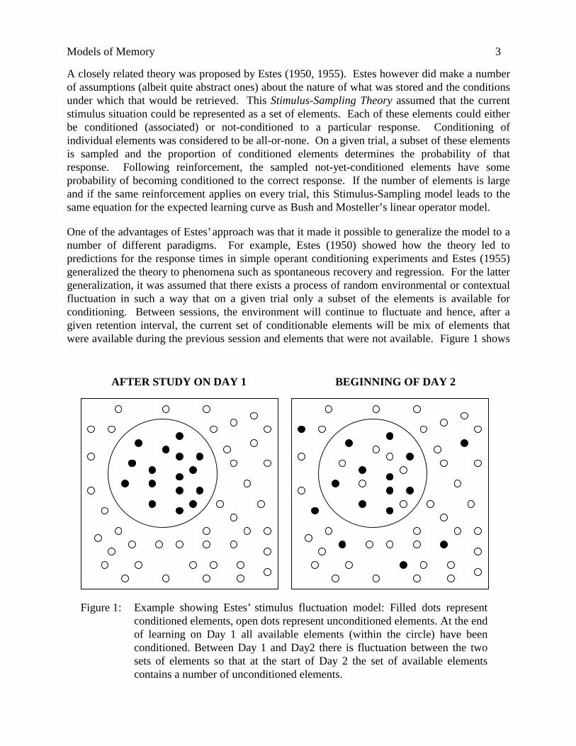
One of the advantages of Estes’ approach was that it made it possible to generalize the model to anumber of different paradigms. For example, Estes (1950) showed how the theory led topredictions for the response times in simple operant conditioning experiments and Estes (1955)generalized the theory to phenomena such as spontaneous recovery and regression. For the lattergeneralization, it was assumed that there exists a process of random environmental or contextualfluctuation in such a way that on a given trial only a subset of the elements is available forconditioning. Between sessions, the environment will continue to fluctuate and hence, after agiven retention interval, the current set of conditionable elements will be mix of elements thatwere available during the previous session and elements that were not available. Figure 1 shows

Figure 1: Example showing Estes’ stimulus fluctuation model: Filled dots representconditioned elements, open dots represent unconditioned elements. At the endof learning on Day 1 all available elements (within the circle) have beenconditioned. Between Day 1 and Day2 there is fluctuation between the twosets of elements so that at the start of Day 2 the set of available elementscontains a number of unconditioned elements.

AFTER STUDY ON DAY 1 BEGINNING OF DAY 2

Models of Memory 4

an example of such a fluctuation process. In this example, training takes place on Day 1 until allavailable elements (those within the circle) have been conditioned (left panel of Fig 1). Howeverbetween Day 1 and Day 2, there is fluctuation between the sets of available and unavailableelements so that at the start of Day 2 (right panel) some conditioned elements in the set ofavailable elements have been replaced by unconditioned elements. It is easy to see that this willlead to a decrease between sessions in the probability of a conditioned response.3 In this example,the probability of a response would decrease from 1.0 (=16/16) at the end of Day 1 to 0.625(=10/16) at the start of Day 2. In this way, spontaneous regression could be explained.Spontaneous recovery would be just the opposite, such that the available elements would all beunconditioned at the end of Day 1 but would be replaced by conditioned elements due tofluctuation during the retention interval; in this way the probability of a response on Day 2 wouldshow a recovery of the conditioned response.

The important point here is that such predictions are possible because the theory provides amechanism (in this case a very simple one) that determines how the system generates a response,rather than just a function that transforms one response probability into another. AlthoughStimulus-Sampling Theory is rarely used these days, the theory has been very influential and maybe viewed as the starting point of modern mathematical modeling of learning and memoryprocesses.

One of the significant modeling developments that came out of the Stimulus Sampling approachwas the use of simple Markov models to describe learning processes. The first (and indeedsimplest of these) was the one-element model proposed by Bower (1961). In this model it wasassumed that there is only a single element for each stimulus that is present on each presentationof that item. On each presentation there is a probability c that the item will be conditioned (orlearned). Since the element will be either conditioned or unconditioned, learning of a single itemwill be an all-or-none event, which is why the model is also known as the all-or-none model. Themodel still predicts a gradual learning curve because such a curve will represent the average of anumber of items and subjects, each with a different moment at which conditioning takes place.The learning process in the all-or-none model may be represented by a simple Markov chain withtwo states, the conditioned or "learned" state in which the probability correct is equal to 1, and theunconditioned state in which the probability correct is at chance level (denoted by g). Thefollowing matrix gives the transition probabilities, the probabilities of going from state X (L or U)on trial n to state Y on trial n+1.

state on trial n+1 P(Correct)L U

state on trial nL

U c c

1 0

1−

1

g

(3)

3 This same model of contextual fluctuation was later incorporated by Mensink and Raaijmakers (1988) in theirapplication of the SAM model to interference and forgetting.

Models of Memory 5

Bower (1961) applied this model to a simple learning experiment in which subjects werepresented lists of 10 paired associate items in which the stimuli were pairs of consonants and theresponses were the integers 1 and 2 (hence this experiment might perhaps be better described as aclassification learning experiment since the subjects have to learn the correct category for eachpair of consonants). The interesting aspect of this application was that Bower did not just look atthe learning curve (which would not be very informative or discriminative) but derived a largenumber of predictions for many statistics that may be computed from the data of such a learningexperiment, including the distribution for the total number of errors, the distribution of the trial oflast error, and the frequencies of error runs. The model fitted Bower’s data remarkably well (seeFigure 2 for an example) and this set a new standard for mathematical modelers.

One of the key predictions of the model was what became known as presolution stationarity: Theprobability of responding correctly prior to learning (or prior to the last error) was constant. Oneof way of formulating this is in terms of the probability of an error being followed by anothererror:

P e en n( )+1 = constant for all n (4)

It may be shown that this presolution stationarity property coupled with one other assumption(such as the distribution of the trial of last error) is a sufficient condition for the all-or-nonemodel. Thus, the crucial property of the all-or-none model is that errors are (uncertain) recurrentevents (Feller, 1957). Batchelder (1975) showed that for this stationarity property to hold, it isnecessary that there are no subject differences in the learning parameter c. To see this, note that ifsubjects do differ, it will be the case that for larger n, only the slower subjects will be included inthe data (the faster subjects will already have learned and will not make an error). That is, theprobability

0.00

0.10

0.20

0.30

0.40

0.50

0 1 2 3 4 5 6 7

k

Pr(

T=

k)

Data

All-or-none model

Figure 2: Observed andpredicted distributions ofthe total number of errorsper subject-item sequence(After Bower, 1961).

Models of Memory 6

P e e c gn n( ) ( )( )+ = − −1 1 1 , (5)

will be based on a different, lower, mean value of c for later trials. Hence, the assumption ofpresolution stationarity is not just crucial, but also quite restrictive. One of the reasons whyBower’s data fitted the model so well (despite its restrictiveness) may have been the relativesimplicity of the experimental task. In the years that followed it became evident that morecomplicated designs would not conform to the predictions of the simple all-or-none model(Bjork, 1966; Rumelhart, 1967).

Notwithstanding the facts that the model was quite simple, that it was rather sparse in itsassumptions concerning cognitive mechanisms, and that it was eventually rejected, it did fulfill animportant function in the "coming of age" of mathematical models for learning and memory: Thedetailed level at which the data were analyzed, and for which predictions were derived, set astandard for future modeling efforts.

In the next ten years, various Markov models were proposed that built upon the all-or-nonemodel. Greeno and Scandura (1966), Batchelder (1970) and Polson (1972) generalized the all-or-none model to transfer-of-training and the learning of conceptual categories (several lists in whicha stimulus item from a specific category is always paired with same response). The basic ideaheld that when consecutive lists are conceptually related, there might be all-or-none learning ontwo levels: the individual item level and the category level. Atkinson and Crothers (1964)extended the model to include the notion of a short-term memory state, a rather importantconceptual/modeling advance as subsequent events demonstrated. Various versions of such amodel have been proposed by a number of researchers, but the basic notion always was that anitem could move from the unlearned state to the short-term state when that item was presented forstudy but could move back to the unlearned state on trials in which other items were studied. Thelearning process can then be described using two transition matrices, one that applies when thetarget item is presented (T1) and one that applies when another item is presented (T2):

L S U

T1 =

L

S

U

d d

wc w c w

1 0 0

1 0

1 1

−− −

( ) ( )

(6a)

L S U

T2 =

L

S

U

f r f r f

1 0 0

1 1 1

0 0 1

( ) ( )( )− − −

(6b)

where L is the state in which the item has been learned, S is an intermediate or short-term state,and U is the state in which the item is not learned.

Models of Memory 7

Although these LS-models still assume that learning eventually results in a state (L) from whichno forgetting would occur (obviously a simplifying assumption), they also introduced a number ofelements that would become important in the following years. For example, the models explicitlydeal with the events between successive study trials and incorporate the notion that additionalstorage (as well as forgetting) may occur on those intervening trials (see T2). Based on thisgeneral approach, Bjork (1966), Rumelhart (1967) and Young (1971) developed (increasinglycomplex) models to account for spacing effects in paired-associate recall, leading to a model thatbecame known as the General Forgetting Theory. Thus, the Markov models shifted from anemphasis on learning to an emphasis on (intertrial) forgetting.

In 1968 Atkinson and Shiffrin produced a model and a model framework that can be thought ofas a natural culmination of these various developments. Their model became known as the’modal model of memory’, partly because it used principles extracted from the rapidly developingstudies of short-term memories to produce a model specifying the relations of short-term to long-term memory. In modeling circles, their theory broke new ground for a different reason: It wentmuch farther than previous theories in quantifying assumed underlying processes of cognition,including rehearsal strategies for short term memory, and retrieval strategies for long-termmemory (Atkinson & Shiffrin, 1968). An important advance was the shift of emphasis from aninexorable march through a limited number of states of memory to a final and permanent learnedstate (as in the Markov models) to an emphasis upon search and retrieval processes from long-term memory (see Shiffrin, 1968, 1970; Shiffrin & Atkinson, 1969; Atkinson & Juola, 1974).Although this model retained an assumption that long-term memory was a (relatively) permanentstate, its addition of retrieval failure as an explanatory mechanism allowed it to handle a far widerrange of phenomena. Another distinguishing characteristic of the Atkinson-Shiffrin theory wasthe fact that it provided both a general framework for analyzing memory processes and also anumber of detailed mathematical models for specific experimental tasks. In all these senses, theAtkinson-Shiffrin model may indeed be said to be the first modern model for human memory.

The Atkinson-Shiffrin model

Although this theory is probably best known as the major representative of what is often referredto as the Modal Model for Memory (Murdock, 1967; see also Izawa, 1999), the distinctionbetween a Short-Term Store (STS) and a Long-Term Store (LTS) was perhaps not the mostimportant or original contribution made by Atkinson and Shiffrin’s model. The frameworkproposed by Atkinson and Shiffrin was based on a distinction between permanent structuralfeatures of the memory system and control processes. The permanent structural features includethe various memory stores: the sensory registers (e.g., iconic and echoic memory), STS and LTS.The other aspect discussed by Atkinson and Shiffrin were the control processes, the operationsthat are carried out to operate on and control memory, such as rehearsal, coding, and retrievalstrategies. Although this is often overlooked in introductory textbooks (see also Raaijmakers,1993) the concept of control processes and how these relate to memory storage and retrieval,made it possible for this Two-Store model to explain the effects of the nature of the study

Models of Memory 8

activities and what subsequently became known as "levels-of-processing" effects (Craik &Lockhart, 1972).4

Atkinson and Shiffrin (see Shiffrin and Atkinson, 1969) assumed that LTS was permanent: onceinformation is stored in LTS is remains there, there is no process that leads to a decay or adecrease in the strengths of the traces in LTS. Although there are exceptions (see e.g.,Wickelgren, 1974) such an assumption is quite common in current models of models of memory.At first sight, this might seem to be strange since one would expect theories of memory to dealwith the essentially universal phenomenon of forgetting. Current theories of memory, however,assume that most forgetting is the result of retrieval failure, either because other information inmemory competes during retrieval with the target information or because the available retrievalcues have changed since the original encoding (e.g., when the retrieval context has changed).Although it is hardly possible to prove such an assumption, it has proved useful and durable, andmost theorists have seen no compelling reason to introduce additional and alternative long-termforgetting assumptions.

In addition to presenting a general framework for human memory, Atkinson and Shiffrin alsoshowed how specific models could be derived within that framework for specific experimentaltasks. In most of these tasks, the situation was such that the usefulness of using a simplemaintenance rehearsal strategy was maximized and more elaborative rehearsal strategies wereless likely to be useful. For example, in one task the participants were presented long series ofpaired associates consisting of a two-digit number and letters from the alphabet (23-H, 47-K).During a particular experimental session only a small set of stimuli was used. The response term(the letter) for a given stimulus term (the number) was varied. The task was to remember whichletter was last paired with a particular 2-digit stimulus. Using such tasks made it possible toinvestigate in detail the workings of simple rehearsal processes in STS.

In sum, the Atkinson-Shiffrin theory may be seen as a prime example of the ’modern’ approach inthis area: the combination of a general theoretical framework and detailed mathematical modelsfor specific experimental tasks. In the next sections we will describe some of the seminaltheoretical frameworks that have been presented in the past 25 years.

Search models

SAM

The SAM theory (Raaijmakers & Shiffrin, 1980, 1981), based on earlier work by Shiffrin (1970),was initially developed as a model for free recall (Raaijmakers, 1979) but was quicklygeneralized to other recall paradigms and to recognition (Gillund & Shiffrin, 1984). The basicframework of SAM assumes that during storage, information is represented in "memory images",

4 Note that the original Atkinson and Shiffrin model already included the notion that rehearsal processes in STSmight be conceptualized as lying on a continuum, with simple or maintenance rehearsal (without the intention toremember) on one end and coding rehearsal (where the intention to remember is most important) at the other end(see Raaijmakers, 1993).

Models of Memory 9

which contain item, associative and contextual information. The amount and type of informationstored is determined by coding processes in STS (elaborative rehearsal). For the usual,intentional study procedures, the amount of information stored in LTS was assumed to be afunction of the length of time that the item or the pair of items is studied in STS.

According to SAM, retrieval from LTS is a cue-dependent process. These cues may be wordsfrom the studied list, category cues, contextual cues, or any other type of information that thesubject uses in attempting to retrieve information from LTS (or that happens to be present in STSat the time of retrieval). Whether an image is retrieved or not, depends on the associativestrengths of the retrieval cues to that image. SAM incorporates a rule to compute the overallstrength of a set of probe cues to a particular image: let S(Qj,Ii) be the strength of association

between cue Qj and image Ii. Then the combined strength or activation of image Ii, A(i), for a

probe set consisting of Q1, Q2, ..., Qm is given by5

A i S Q Ij ij

m

( ) ( , )==∏

1

(7)

The key feature of Eq. 7 is that the individual cue strengths are combined multiplicatively into asingle activation measure. This multiplicative feature focuses the search process on those imagesthat are strongly associated to all cues, the intersection of the sets of images activated by each cueseparately. For episodic memory paradigms, the cue set will always contain a context cue(representing the list context) that enables the search process to focus on the particular list that isbeing tested.

In recall tasks, the search process of the SAM model is based on a series of elementary retrievalattempts (see the flowchart in Figure 3). Each attempt involves selecting or sampling one imagebased on the activation strengths Ai. The probability of sampling image Ii equals the relative

strength of that image compared to all images in LTS:

P IA i

A kS i( )( )( )

=∑

(8)

Sampling an image allows recovery of some of the information from it. Note that the systemdoes not simply retrieve a copy of the item. Rather, it is assumed that a set of features orfragments are activated and that the system has to reconstruct the item based on the activatedfeatures. Hence, there is a constructive element in recall. For simple recall tasks where a singleword has to be recalled, the probability of successfully recovering the name of the encoded wordafter sampling the image Ii is assumed to be an exponential function of the sum of the strengths of

the probe set to the sampled image:

5 For simplicity we ignore the assumptions regarding weighting of cues (in effect we are assuming, as in many SAMapplications, that these weights are all equal to 1).

Models of Memory 10

P I S Q IR i j ij

m

( ) exp ( , )= − −

=

∑11

(9)

In the simplest variant of this model, the probability of recall, assuming Lmax retrieval attempts

with the same set of cues, is given by the probability that the item was sampled at least once,times the probability that recovery was successful:

( )[ ]P I P I P Irecall i s i

L

R i( ) ( ) ( )max= − −1 1 (10)

Assuming that each cycle takes the same amount of time T, the latency distribution for correctresponses is equal to:

P RT l TP P

Ps

ls

sL( )

( )

( ) max= ⋅ =

−− −

−1

1 1

1

for l=1, .... Lmax (11)

Special assumptions are necessary when an image has previously been sampled using one or moreof the present cues but its recovery did not lead to successful recall. In that case, recovery isbased only on the "new" components of the sum in Eq. (9), corresponding to cues that were notinvolved in the earlier unsuccessful retrieval attempts (see Gronlund & Shiffrin, 1986).

Start

Sample image

Recoverysuccessful?

Correctitem?

Give up?

Stop Output

Yes

No

No

No

Yes

Figure 3: Flowchart representing theSAM retrieval process in a cuedrecall task.

Models of Memory 11

The above equations apply directly to cued recall. More complicated recall paradigm such as freerecall can be handled in a similar way, by making assumptions about the retrieval strategy that isused. In the standard SAM model for free recall, it was assumed that the search starts using onlythe context cue (the only information available). As the search proceeds any item that is retrievedis used as an additional cue (for a maximum of Lmax retrieval attempts). If this item+context

search is not successful, the system will revert to using only the context cue.

If the retrieval attempt is successful, the associative connections between the probe cues and thesampled image are strengthened. Thus, SAM assumes that learning occurs during retrieval aswell as during study. This assumption leads to a kind of retrieval inhibition, because it decreasesthe probability of sampling other images. If the retrieval attempt is not successful, a decision ismade about whether to continue, either with the same set of cues or with some other set of cues.The decision to terminate the search process is usually based on the number of unsuccessfulsearches, although other types of stopping rules are also possible.

Although the SAM model assumes that the process of activating information is basically the samein recall and recognition, there are some important differences between these two processes.Search models are not generally proposed as a primary basis for recognition because they havedifficulty predicting similar response times for ’old’ and new’ recognition decisions. Thus Gillundand Shiffrin (1984) proposed that recognition is based on the overall activation induced by theprobe cues. That is, the overall activation, ∑ A(k), defines a familiarity value that is used in themanner of signal-detection theory to determine the probability of recognition. This notion of"global familiarity" introduced by Gillund and Shiffrin has become a general property of mostcurrent recognition models (often termed "global memory models" for that reason). In order toderive predictions, some assumption is also needed about the variance of the strengthdistributions. Typically, the standard deviation is assumed to be proportional to the meanstrength value (Gillund & Shiffrin, 1984; Shiffrin, Ratcliff, & Clark, 1990).

Of course, alternative and more complex models for recognition might be constructed within theSAM framework. One obvious approach (much explored in recent years) assumes recall is usedin tandem with familiarity to determine recognition. An early form of this approach was a two-stage model (as in Atkinson & Juola, 1974): Two criteria are used such that a fast ’new’ responseis given if the familiarity is below the lower criterion and a fast ’old’ response is given if thefamiliarity is above the upper criterion. If the familiarity lies between these two criteria, a moreextended search process (as in recall) is undertaken. Alternatively, it might be assumed that thereare two parallel routes in which one route would be based on familiarity and one on a recall-likeprocess. In general (especially when dealing only with accuracy data), dual-route models makepredictions similar to those from single-route models to the degree that familiarity is abovecriterion for items that are successfully recalled.6

According to SAM, contextual information is always encoded in the memory image, and forepisodic-memory tasks, context is one of the retrieval cues. Changes of context between study

6 This seems to be in conflict with the recognition failure of recallable words phenomenon (Flexser & Tulving, 1978).However this effect depends on the use of a specific paradigm and does not necessarily generalize to a task in whichrecall is a subprocess within a recognition task.

Models of Memory 12

and test play an important role in the prediction of forgetting phenomena. Such changes may bediscrete or occur in a more gradual way. Discrete changes are typical for studies that explicitlymanipulate the test context (e.g., Godden & Baddeley, 1975; Smith, 1979).7 On the other hand,gradual changes may occur when the experimental paradigm is homogeneous (as in continuouspaired-associate learning). In such cases, context similarity between study and test will be adecreasing function of delay.

Mensink and Raaijmakers (1988, 1989) proposed an extension of the SAM model to handle time-dependent changes in context. The basic idea, adapted from Stimulus Sampling Theory (Estes,1955), is that a random fluctuation of elements occurs between two sets, a set of available contextelements and a set of (temporarily) unavailable context elements. The contextual strengths at testare a function of the relationship between the sets of available elements at study and test.Mensink and Raaijmakers (1989) showed how some simple assumptions concerning thefluctuation process yield equations for computing the probability that any given element is activeboth at the time of storage and at the time of retrieval. A more elaborate analysis of contextualfluctuation processes and its application to free recall was recently proposed by Howard andKahana (1999, see also Kahana, 1996). They showed how such a notion could be used within aSAM-like model to explain a number of effects (such as long-term recency) that would bedifficult to explain under the constant context assumption that was used in Raaijmakers andShiffrin (1980).

The SAM theory has been quite successful. The SAM approach to recall and recognition hasbeen shown to provide relatively straightforward explanations for a number of standard findings(such as the effects of list length, presentation time, serial position effects) as well as a number offindings that previously were considered quite problematic (e.g., the part-list cuing effect [seeRaaijmakers & Phaf, 1999], spacing effects [see Raaijmakers, 1993], the differential effects ofnatural language frequency and of context changes on recall and recognition [see Gillund &Shiffrin, 1984] and the set of results that had caused problems for the traditional InterferenceTheory of Forgetting [see Mensink & Raaijmakers, 1989]).

Ratcliff, Clark and Shiffrin (1990), however, discovered a phenomenon, called the "list-strengtheffect", that could not be explained within SAM without making additional assumptions. Thisrefers to the effects of strengthening some list items on memory for the other list items. Ratcliffet al. (1990) showed in a series of experiments that strengthening some items on the list has anegative effect on free recall of the remaining list items (as one would expect for any modelbased on relative strengths) but has no effect on cued recall or even a positive effect onrecognition performance. This stands in contrast to the list-length effect: adding items to a listdecreases both recall and recognition performance.

In a prototypical experiment on the list-strength effect, three conditions are compared: a pure listof weak items (e.g. brief presentation time, single presentation), a pure list of strong items, and amixed list consisting of both weak and strong items. Of course strong items do better than weakitems, both in pure and mixed lists, and for free recall, cued recall, and recognition. However,

7 The effect upon memory of a discrete context change appears to depend on the degree to which context informationis integrated with content information, as explicated in the ICE theory (e.g. Murnane, Phelps, & Malmberg, 1999).

Models of Memory 13

the critical aspect is that strong items in mixed lists are not recognized better than in pure lists (infact they are a little worse). Similarly, weak items in mixed lists are not recognized worse thanon pure lists (in fact they are a little better). Since the relative strength of a strong item in amixed list is larger than in a pure list (and similarly for a weak item on a pure weak list comparedto a weak item in a mixed list), a model like SAM would have predicted a difference inrecognition performance. Because adding items to a list does harm performance, one mightexpect a similar effect if one strengthens other items.

Shiffrin et al. (1990) showed that a variant of the SAM model could handle the results if onemakes a differentiation assumption: The better an item is encoded, the more clear are thedifferences between the item information in its image and the item information in the test item.Conversely, the better an item is encoded, the stronger will be the match between the contextinformation encoded in its image and the context information used in the test probe. Becausestrength of activation in SAM is determined by the product of context and item strength, the neteffect of these two opposing factors is to cancel, approximately. Because both cued recall andrecognition use both item and context cues at test, differentiation produces the observed null list-strength effect for these paradigms. On the other hand, because many test probes during freerecall use context cuing only, a list strength effect is predicted for this case, as observed.Although this differentiation assumption may have seemed a bit ad-hoc when first introduced, theyears since have shown the difficulty of finding any alternative account of the list-strengthfindings, and the differentiation assumption is generally accepted, whatever the modelframework.

Although the differentiation assumption was an important and helpful addition to SAM, a numberof other problems remained. One of these concerned the so-called "mirror effect" in recognition.This effect refers to the finding that many factors that increase the probability of a ’hit’ (saying’yes’ to a target item) also decrease the probability of a ’false alarm’ (saying ’yes’ to a distractoritem), as documented extensively by Glanzer and his colleagues (e.g., Glanzer & Adams, 1985;Glanzer, Adams, Iverson, & Kim, 1993). Thus, the order of the conditions for the probability ofsaying ’yes’ to distractors is the mirror image of the order for these same conditions for theprobability of saying ’yes’ to target items. For example, although low-frequency items are morelikely to be correctly rejected than high-frequency items, LF target items are also more likely tobe correctly recognized than HF targets. Such mirror effects are difficult to explain for any modelthat bases the probability of saying ’yes’ on a "strength"-like measure. Although mirror effectsmight be handled by assuming different criteria for HF and LF items, such a solution is inelegant,and it has been difficult to find coherent explanations for the posited movement of the criteriaacross conditions.

Recently, Shiffrin and his co-workers have developed a new model, REM, that retains many ofthe best elements of SAM, but provides a principled solution for the mirror effect, and for anumber of other previously unexplained memory phenomena.

Models of Memory 14

REM

The REM (Retrieving Effectively from Memory) model started out as a model for recognitionmemory (Shiffrin & Steyvers, 1997). Because global familiarity models faced problemsexplaining the mirror effect, a solution had to be found that would provide a more rational basisfor criterion placement. Shiffrin and Steyvers (1997) realized that the assumption that thememory system behaves as an optimal decision making system might produce a model capable ofsolving this problem.

In REM, memory images are represented as vectors of feature values, e.g. <3,1,3,7,3,2,1,....>.The numbers represent the frequency of a particular feature value. The probability that a featureV has value j is assumed to be given by the geometric distribution8:

P V j g g jj( ) ( ) ,= = − = ∞−1 11 � (12)

That is, not all feature values are equally likely. Now, suppose an item is studied. As a result ofstudy, an episodic image (of item and context features) is stored in memory. This episodic imagewill be error prone, i.e. some features will not be stored correctly, and some will not be stored atall. The better or the longer an item is studied, the higher the probability that a given feature willbe stored.

On a recognition test, old and new items are presented and the subject is asked to indicatewhether the test item is old (from the list) or new. It is assumed that the system compares theretrieval probe features to those stored in episodic memory images, noting the matches andmismatches to the features in each image. The system then uses a rational basis for generating aresponse: It chooses whichever response has the higher probability given the observed featurematches and mismatches in all the memory images. Thus, if there is an episodic image inmemory that is quite similar to the test item, producing many matching features, the probabilitythat the test item is old will be high. Mathematically, the decision criterion is given by theposterior odds ratio which according to Bayes’ rule may be written as the product of the priorodds and the likelihood ratio:

( )( )

( )( )

( )( )Φ = = ×

P old data

P new data

P old

P new

P data old

P data new

|

|

|

|(13)

(when the prior probabilities of old and new items are equal, as is the case in most studies, theposterior odds is simply the likelihood ratio itself). It can be shown (see Shiffrin & Steyvers,1997) that in REM, the likelihood ratio is given by the average likelihood ratio for the individuallist traces (assume L episodic images are compared to the test probe): :

8 It should be noted that this assumption is not essential for the REM model. Most predictions do not depend on thenature of this distribution.

Models of Memory 15

( )( )Φ = =∑ ∑1 1

L L

P D old

P D new

j

jjj

j

|

|λ (14)

Hence, an "old" response would be given if Φ > 1. This result is of course quite similar to theSAM recognition model if one substitutes the likelihoods in REM for the SAM activation values.A critical difference concerns response criteria: In SAM the familiarity values are on an arbitraryscale that changes with conditions, and a response criterion must be chosen differently for eachcondition. In REM the odds have a natural criterion at 1.0. Although the participant couldchoose a response criterion different from 1.0 if conditions warrant, the default criterion of 1.0produces a mirror effect. This prediction and others suggested that the REM model forrecognition was indeed qualitatively better than SAM, despite the many similarities.

The similar role played by likelihood ratios in REM and retrieval strengths in SAM suggested thatthe SAM recall model could be ported to REM by substituting likelihood ratios for strengths.Such an approach has the desirable feature that most (if not all) of the SAM recall predictionshold for REM as well. In carrying out this procedure, it was discovered that the distributions ofthe likelihood ratios were much more severely skewed than the retrieval strengths in SAM. Oneundesired result of this fact was a tendency to sample the highest strength image with too high aprobability. For this reason, sampling in recall in REM is assumed to be based on a powerfunction of the likelihoods (see Diller, Nobel, & Shiffrin, 2001):

P IS ii

k

( ) =∑

γ

γλλ

(15)

Diller et al. (2001) show that such a model accurately describes the response time distributions incued recall. More generally, these authors show that an appropriately tailored REM model givesa good simultaneous fit to the accuracy and response time data in both cued recall andrecognition.

It is worth highlighting one major difference between the SAM activation values and the REMlikelihood ratios. In REM, the likelihood ratio for an individual trace is a function of the numbersof both matching features and mismatching features (see Shiffrin & Steyvers, 1997):

λ αβ

αβj

m qj j

=

−−

1

1 , (16)

where α is the probability of a match given storage for the correct trace, β is the probability ofmatch given storage for an incorrect trace (α must obviously be larger than β), and mj and qj arethe number of matches and mismatches respectively for trace j. Thus, the higher the number ofmatching features, the higher the likelihood,and the higher the number of mismatching features,the lower the likelihood. Consider what this implies for the likelihood ratio for a strengthenedimage when a different item is tested. More features will be stored in the ’stronger’ image, but

Models of Memory 16

these will generally mismatch the test probe (because the image and test probe do not match).The likelihood ratio for the stronger image therefore tends to be lower. This mechanism may beseen as an implementation of the differentiation hypothesis: Stronger traces are more easilydiscriminated from the test item than weak items. Shiffrin and Steyvers (1997) showed that theREM model could indeed account for the list-strength results.

The comparison of SAM to REM in the domain of episodic recognition provides a mostilluminating look at two rather different approaches to modeling. The SAM model was generatedin much the way that most psychology models have been developed over the past 50 years:knowing the data patterns to be predicted, plausible cognitive mechanisms were hypothesized,and implemented with functional forms that intuition suggested would produce the observed datapatterns. A certain period of tuning of the model then ensued, as is usually the case, becauseintuitive predictions are notoriously error prone. In the case of SAM, the functional formsincluded, as an example, the assumption that cues would combine multiplicatively, enabling thesystem to converge upon images in the intersection of the items similar to each cue separately.The REM model was developed somewhat differently: A few structural limitations wereassumed at the outset, chiefly the assumption that images are stored incompletely and with error.Then the model was derived rather than assumed, under the assumption that the structure of thetask was known, and that all the information in images was available for optimal decisionmaking. The functional form of the equations governing REM were therefore derived rather thanassumed. It should be emphasized that there is no necessary reason why this approach should besuperior, or that the cognitive system should necessarily be designed in optimal fashion to carryout any given task. The fact that it seemed to work well in the present instance does point out thepotential utility of the approach, and gives the modeler another weapon in his or her theoreticalarsenal.

Although the REM model was developed initially in the domain of episodic recognition memory,and represented an improvement upon SAM in that domain, its primary contributions lay indifferent spheres: generic (or semantic) and implicit memory. The model provided a mechanismthrough which episodic images could be accumulated into lexical/semantic images, over manyrepetitions across developmental time, and enabled retrieval from such memories with the samebasic processes that operate in episodic tasks. It is assumed (see Schooler, Shiffrin &Raaijmakers, 2001) that when an event is first stored, a noisy and incomplete (episodic) image isstored in memory. When that event is repeated, a new episodic image will be stored. However, ifthe new image is sufficiently similar to the previous stored image, information may also be addedto that previous image. Thus, repetitions will gradually lead to an increasingly complete image,that may be termed a lexical/semantic image. This accumulated image will contain perceptual,semantic, and contextual features. However, since the contextual information will come frommany different contexts, the activation of the lexical/semantic image will not depend on anyparticular test context, and sampling of such an image will not produce a sense of any oneepisodic event. Tthe lexical/semantic images will in effect become context-independent, notbecause they fail to encode context, but because they encode too many contexts. Thus, althoughREM incorporates a distinction between episodic and semantic memory, both have a commonorigin and follow the same basic rules.

Models of Memory 17

The retrieval processes assumed to operate in explicit memory can in turn be used to describeretrieval from lexical-semantic memory: A probe vector of features is compared to the set oflexical-semantic images, and likelihood ratios calculated for each. These likelihood ratios canthen be summed, for example to make a lexical decision (word/nonword decision), or used as abasis for sampling for a variety of recall-based tasks such as naming or fragment completion.

It is only a minor extension to use these same processes to model implicit memory effects.Implicit memory refers to findings that recent study of a word enhances (or at least alters)performance on a subsequent generic memory test, where the subsequent test may beaccomplished without reference to episodic memory (and even without explicit realization thatthe previously studied words are relevant). For example, a lexical decision given to the word’table’ may be speeded by study of table in a prior list. Such effects are often termed ’repetitionpriming’. In order to explain repetition priming effects, REM borrows the previously stated ideathat study produces storage not only of an episodic image but also additional storage in apreviously stored similar image, in this case, the lexical/semantic image of the studied word. Onerefinement of this idea is needed: The added information is restricted to information not alreadystored in the lexical/semantic image. Thus item information in the lexical/semantic image suchas its core meaning, which is already stored, is unaffected by a recent study event. However,perceptual (e.g. font) and context information which is unique to the current study episode isadded to the lexical/semantic image.

These storage assumptions lead naturally to the prediction of repetition priming, as long as thetest probe utilizes any of the information that had been added to the lexical/semantic image. Thusif current context is used as part of the test probe, which may be inevitable even in tasks that donot require context cuing, then the match of this information to that stored in the lexical/semanticimage of the studied word will increase the likelihood ratio for that image, and produce priming.One example is presented in Schooler et al. (2001). They present a REM-based model to accountfor priming effects in perceptual identification and in particular the results obtained by Ratcliffand McKoon (1997). Ratcliff and McKoon had participants study a list of words. Subsequentlythe participants saw a briefly flashed and masked word, and then received two choice words, oneof which had been the one flashed (the target) and one not (the foil). If a choice word had beenstudied in the earlier list, it is said to have been primed. The target, the foil, both, or neitherchoice could have been primed, in different trials. For example, during study the word LIEDmight be presented. At test, the word LIED is briefly flashed and then two alternatives, say LIEDand DIED, are presented for a choice. When the choices are perceptually similar (such as LIEDand DIED) priming the target increases its choice probability, but priming the foil does so as well.If the choices are dissimilar (say LIED and SOFA), there is little effect of priming.9

Ratcliff and McKoon (1997) argued that this pattern of results poses a challenge for existingmodels of word identification because these models assume that "prior exposure to a wordchanges some property of the representation of the word itself" (Ratcliff & McKoon, 1997, p.339). They proposed a Counter Model in which the system assigns perceptual evidence to each

9 With slightly different instructions, Bowers (1999) was able to obtain priming for dissimilar alternatives as well.The difference may depend on differential tendencies for the subjects to use episodic memory access to help carry outthe identification task.

Models of Memory 18

of the two choice words. Prior study leads to bias in the system in such a way that a countercorresponding a studied word tends to "steal" counts from neighboring counters (for similarwords). Schooler et al. (2001) however showed that this pattern of results can be also explainedin REM if one assumes that prior study leads to the storage of a small amount of new contextualinformation (i.e., prior study does change "some property of the representation"). The idea issimple: The extra matching context features for the studied item increase the likelihood ratio forchoice of its lexical/semantic image over that for the alternative word. For similar alternatives,only a few visual features are diagnostic since most letters areshared between the choices (e.g. theIED part of the choices are not relevant when choosing between LIED AND DIED); in this casethe extra likelihood due to prior study has a large effect. For dissimilar alternatives many or allvisual features are diagnostic so the same extra likelihood has a smaller relative effect.

At this moment, work on the application of REM to other implicit and semantic memoryparadigms (such as lexical decision [Wagenmakers et al., 2001]) is still in progress. However, itseems likely that the REM model will be able to use the mechanisms outlined above to explainseveral of the most basic findings in implicit memory. For example, the finding that perceptualimplicit memory tasks (word identification, lexical decision) are usually unaffected by levels-of-processing variations in the study task that do have a clear effect on explicit memory, can beexplained by pointing out that such variations mostly affect the number and nature of thesemantic features that are stored in episodic traces, and these features are not the ones added tothe lexical/semantic traces since they will usually already be present in those traces. In addition,since whatever semantic or associative information is present in STS when the target item ispresented, will be unrelated to the semantic/associative features of the lexical/semantic trace, aprior semantic study task will not affect the match between the presented item and the targetlexical trace. As another example, amnesic patients that have a very deficient explicit memoryoften show relatively normal implicit memory performance; in REM the implicit benefit is basedon altered activation of lexical-semantic traces, and these patients are known to exhibit fewdeficits in semantic memory tasks requiring access to those traces (e.g., standard wordidentification tasks).

Only time will tell whether REM, or alternative models, will be successful in their attempt tointegrate explicit memory, semantic memory, and implicit memory within a single theoreticalframework. However, this goal is a major goal of current research , and in this respect, thesemodels have come a long way from the simple Markovian models of the 1960s.

The MINERVA 2 Model

Hintzman (1986, 1988) developed a memory model that is based on global familiarity, somewhatlike the SAM and REM models for episodic recognition. This model, MINERVA 2, has beenapplied primarily to category learning and recognition memory. A basic goal of the model is toprovide an explanation for memory for individual experiences (episodic memory) and moregeneric or semantic memory within a single system. The model assumes that memory consists ofa large set of episodic traces. It is assumed that each experience produces a separate memorytrace. Memory traces are represented as lists of features or vectors. When an item is studied, anew memory vector for that item is formed. Each feature is independently encoded withprobability L, a learning rate parameter. Features are encoded as +1 or -1. If a feature is not

Models of Memory 19

encoded it is set to 0. When a probe cue is presented, it is compared in parallel to all memorytraces. The amount of activation of any particular trace is a nonlinear function of the similarity tothe probe cue, where similarity is determined by numbers of matching and mismatching features.Overall activation is given by the summed similarity, and is used to make a recognition decision.

In MINERVA 2, a generic or semantic memory is produced by combining or summing a largenumber of individual episodic traces. The basic difference between such an approach to semanticmemory and the one represented, say, by the REM model, is the representation oflexical/semantic memory. REM assumes a separate set of lexical/semantic images, but inMINERVA 2 the semantic traces are computed at the time of retrieval and not stored separately.

For recognition, a test item’s vector is compared with each vector in memory and a similarityvalue is computed using the following equation:

S PT Ni j ijj

N

r==∑

1

(17)

where Pj is the value of feature j of the probe, Tij is the value of the corresponding feature in tracei and Nr is equal to the number of relevant features (i.e., those that are encoded is both the probeand the trace). Thus, the similarity is based on the inner product of the two vectors (also termedthe dot product). The inner product is just the sum across vector positions of the product of thecorresponding entries, and is a single real number. The activation value for trace i is given by

A Si i= 3 . (18)

Thus, the activation rapidly declines as the similarity to the probe decreases. Next, all activationvalues are summed to provide an overall measure of match called "echo intensity". If this value isgreater than a criterion value, an "old" response is produced; if it is less, a "new" response isproduced. Hence, MINERVA 2 is another example of a global familiarity model. MINERVA 2has also been successfully applied to confidence data, and frequency judgment data, by assumingthat such judgments are determined by the value of summed activation obtained on a trial:Appropriate criteria are set that determine the desired responses.

In order to allow recall to be carried out, the model assumes that a specific vector is constructedfrom the activated traces. To be precise, the retrieved vector (called the echo) is the sum of alltrace vectors, each weighted by its activation value:

C ATj i iji

M

==∑

1

(19)

where Cj is the value for feature j in the echo. Because Ai rapidly declines as the similaritydecreases, the echo will be mostly determined by those traces that are similar to the probe cue.How is this echo used to carry out recall? Consider cued recall as an example. Suppose the twowords studied together (say, A and B) are stored in a single concatenated vector, back to back(A,B). MINERVA 2 has a property that might be called pattern completion: Whenever part of atrace is used as a probe (say the test word, A), the echo will also contain retrieved values for the

Models of Memory 20

features that are missing in the probe. These filled in features will tend to be determined by thetraces with the highest activation, i.e. those similar to the test word, A. Chief among these will ofcourse be the trace encoding the test word (A,B). Hence the echo will tend to have featuressimilar to the response word in the test word’s trace (i.e. B). This is a standard mechanism forrecall that also figures prominently in several connectionist models for memory (see below). Ofcourse, the retrieved trace is actually a composite of many traces, so some mechanism is neededto extract some particular item from the composite. That is, some way is needed to ’clean up’ thecomposite. This might be done in several ways (see Hintzman, 1986, 1988). Under somecircumstances, the retrieved vector can be recycled as a new retrieval cue, and a series of suchcycles can produce a cleaned up and interpretable response word. In other cases, it wouldprobably be necessary to compare the response vector to words in a separately stored lexicon.

For recognition, the model makes many of the same predictions as other global familiaritymodels. It predicts many of the standard experimental results such as the effects of repetition andstudy time. However, as is the case for most of the other global familiarity models, it does notaccount for the list-strength results and mirror effects that were the primary motivation behind thereplacement of the SAM model for recognition by the REM model. To handle list-strength whatwould be needed is some kind of mechanism similar to the differentiation assumption. Also, themodel has not been tested in a thorough way in recall paradigms. On the other hand, the modelwas the first explicit mathematical model that incorporated the assumption that semantic memorytraces might not be stored separately from episodic traces, but instead computed at the time ofretrieval. This is in many ways an attractive proposal whose power in explainingsemantic/implicit memory findings should be explored further.

It should be mentioned that the first application of MINERVA 2 was to categorization (1986),rather than recognition (1988). It is noteworthy that this model can handle significant findings inboth domains, and indeed a good deal of recent effort by a number of investigators has beendevoted to linking memory and categorization models in a common framework (e.g. Nosofsky,1988). It is natural to link the two because summing activation across the exemplar traces from agiven category can be viewed as providing evidence for that category. Unfortunately, anydiscussion of categorization models takes us well beyond the coverage of this chapter.

Associative Network Models

The idea that activation in memory is based on spreading of activation over a network ofinterconnected nodes and that this is the principal mechanism of associative memory, becamepopular in the 1970s when it was introduced as a framework for semantic memory. Collins andLoftus (1975) and Anderson and Bower (1973) used this idea to explain findings in sentenceverification tasks. Following these initial proposals, the spreading activation notion becamewidely used by researchers in semantic memory to explain findings such as associative orsemantic priming (i.e., the finding that performance on a target item is faster or more accuratewhen that item is preceded by an associatively or semantically related item).10 However, in most

10 Recent years have also seen the introduction of the related concept of spreading inhibition (e.g. Anderson &Spellman, 1995).

Models of Memory 21

of these uses of the spreading activation concept, predictions were derived only very loosely. Inorder to enable exact predictions the general notion of spreading activation has to be incorporatedin a quantitative framework. Several of these frameworks have been developed over the past 30years. In this section we will focus on one well-known example of a spreading activation model,Anderson’s ACT model (Anderson, 1976, 1983b, 1993). The ACT theory (Adaptive Control ofThought) is really a very general cognitive architecture that is not just a framework for memorybut a system in which models may be constructed for all cognitive tasks, including problemsolving, acquisition of cognitive skills (including the acquisition of skills in physics, geometry,computer programming, etc.), learning, language and semantic memory. The architectureconsists of a working memory, a declarative memory system and a procedural memory system.The latter is modeled as a production system, consisting of a large set of both generic as well asspecific production rules that act on the contents of the working memory. However, in thissection we will restrict our discussion to the models that have been derived within ACT for (long-term) memory.

The ACT model (1976-1983)

In the original ACT model (Anderson, 1976), long-term memory was assumed to consist of alarge set of nodes and links connecting these nodes. The nodes represented basic concepts orcognitive units and the links represent semantic or episodic relations. Whenever two items arestudied together in a memory task, a link between the corresponding nodes may be formed. Insuch a model, retrieval of a target item B from a cue item A is accomplished if the activation fromthe node representing A spreads to item B and activates the node representing B (or sends enoughactivation to B to pass an activation threshold). In such a model, nodes are either active orinactive.

In the 1976 version of ACT, the spreading of activation is determined by the (relative) strength ofthe links. For example, suppose that after study of A-B a link connecting these is formed withstrength s. If A is later presented as cue, the probability of activating B in the next unit of time isa function of s/S, the relative strength of the A-B link compared to all other links emanating fromA. Once any node (say, B) does become active, it begins in turn to activate nodes to which it islinked. Of course, some decay of activation has to occur in such a model to prevent eventualactivation of all nodes in memory. In the present model this is prevented by assuming that after Dunits of time, all activated nodes are deactivated (unless they are placed in a kind of buffer orshort-term store).

Because nodes and links are activated in an all-or-none manner, the response latency isdetermined by the time it takes to activate the target node. The larger the distance between thecue and the target (in terms of the number of links in the path from cue to target) the longer theresponse time will be. However, Ratcliff and McKoon (1981) showed in a primed lexicaldecision task that this is not the case. They demonstrated that the semantic distance between theprime and the target does not affect the time at which the facilitation due to priming begins tohave its effect although it does affect the magnitude of the facilitation. In response to suchfindings, Anderson (1983a,b) developed a continuous activation model as an alternative to the all-or-none model.

Models of Memory 22

In the continuous model, the activation values for the nodes vary continuously. Further, the levelof activation is used to determine whether a memory trace has been successfully retrieved. Thatis, the amount of activation that spreads from A to B is determined by the relative strength ofnode B (compared to all other nodes connected to A), and the probability and latency of retrievingtrace B are a function of B’s activation. To explain the Ratcliff and McKoon (1981) data (andother data), the spread of initial activation occurs extremely rapidly, even to distant nodes. Thus,the notion of spreading activation changed from gradually activating connected nodes (i.e., distantnodes take longer to activate) to a dynamic model in which the activation spreads rapidly over thenetwork but in varying degrees (i.e., distant nodes have a lower level of activation).

Anderson (1981, 1983a) applied this model (also referred to as ACT*) to a number of memoryphenomena. It is assumed that during storage memory traces are formed in an all-or-nonemanner. In addition, each trace (once formed) has a strength associated to it. The strength ofthese traces is determined by such factors as the number of presentations and the retentioninterval. More specifically, the trace strength (S) for a trace that has been strengthened n times isgiven by

S tib

i

n

= −

=∑

1

(20)

where ti is the time since the i-th strengthening and b is a decay parameter (between 0 and 1).This assumption agrees with the power law of forgetting (for n=1).

These strengths determine the amount of activation that converges on the trace from associatednodes. Thus, in a paired-associate recall situation, where the subject learns a list of pairs A-B, itis assumed that the trace encodes the information that this pair was presented in this context. Attest, the response will be retrieved if (a) such a trace has indeed been formed, and (b) it can beretrieved within a particular cutoff time. Retrieval time is assumed to follow an exponentialdistribution with a rate parameter that depends on the activation of the target trace. Thisactivation is assumed to be equal to the sum of the relative strength of the target trace (relative toother traces associated to the cue item) and the relative strength of the association between thecurrent context and the target trace (this strength is a function of the number of study trials on thelist).

One prediction of ACT that has received a lot of attention is the so-called fan-effect. This effectrefers to the prediction that the amount of activation that spreads from A to B is a function of thenumber of links emanating from A (or the fan of A). Similarly, in order to verify a sentence suchas "The hippie is in the park" (i.e., to decide whether this sentence is ’true’, is one of the sentencesstudied previously), the response latency is a function of the "fans" of "hippie" and "park": themore sentences have been studied with "hippie" as the subject, the more time it takes to recognizesuch a sentence. Similarly, the more sentences have been studied with "park" as the location, themore time it takes to recognize such the sentence. These predictions were verified in severalexperiments (see e.g. Anderson, 1974). Note that this fan effect is similar to the list length effectthat has been tested extensively in cued recall and recognition.

Models of Memory 23

Anderson (1981, 1983a) also showed that the ACT* model accurately explains a number ofinterference results. One interesting result that follows from the ACT* model is that probabilityof correct recall and latency are differentially affected by interference manipulations. Probabilityof correct recall is determined by two factors, the probability that a link has been formed betweenthe cue item and the target trace (basically a function of the number of study trials, i.e. theabsolute strength of the trace), and the number of other traces associated with the cue item (i.e.,the relative strength of the trace). The latency of correct responses, however, does not depend onthe absolute strength but only on the relative strength. Anderson (1981) showed that this impliesthat even if the probabilities of correct recall are matched between an interference condition andthe control condition, there will still be an interference effect on the latency. This prediction wasindeed verified. Using similar reasoning it may be shown that the ACT* model makes thecounterintuitive prediction that in an unpaced proactive interference paradigm (A-B, A-Dcompared to an C-B, A-D control condition) in which the second list is learned to a fixedcriterion, proactive facilitation should be observed. This prediction follows from the fact that atthe end of second-list learning the absolute strength for the interference condition should behigher if both lists are learned to the same criterion (in order to compensate for the lower relativestrength). It can be shown (see Anderson, 1983a, p. 269) that this implies that after a delay, thetotal activation for the target trace will be higher in the interference condition than in the controlcondition. Anderson (1983a) reports results from his laboratory that confirm this counterintuitiveprediction.

Despite its successes, there are still a number of problems in ACT* that have yet to be resolved.One of the most important ones is that the model does not really have a mechanism to predict thelatencies of negative responses. For example, in the sentence verification experiment, the latencyto determine that a sentence of the form "the A is in the B" was not presented on the study list,seems to be equally affected by the fans of A and B even though there obviously is no path thatlinks A and B (after all, A and B were not presented together). Anderson makes the ad hocassumption that the latency of a negative response is given by the latency of a positive responsefor the same experimental condition plus some constant. Although this fits the pattern of theresults, such an assumption is hard to defend within ACT*.

As mentioned previously, the notion of spreading activation has been very popular inexplanations of associative priming. McNamara (1992a,b, 1994) has made a detailedinvestigation of the application of ACT* to a variety of results from associative priming tasksincluding the prediction of mediated priming: the finding that there is also a priming effect fromLION to STRIPES. Such a result can be explained as being due to the activation spreading fromLION to TIGER and from TIGER to STRIPES. Such a result seems to be strong evidence for thenotion of spreading activation. However, McKoon and Ratcliff (1992) showed that this resultmight also be explained within their compound cue model for lexical decision (see Ratcliff &McKoon, 1988), a model that is based on the global familiarity mechanism used in the SAMmodel for recognition. In the 1990s, the issue of whether associative priming is best explained byspreading activation or by compound cue mechanisms was heavily debated in a large number ofpapers by McNamara and Ratcliff and McKoon. However, there does not seem to have been aclear resolution.

Models of Memory 24

The ACT-R model

In the early 1990s, Anderson (1993) developed a new version of ACT, called ACT-R (ACT-Rational). In many ways, the ACT-R model is similar in spirit to the previous ACT models. Asin the previous version, the cognitive architecture consists of a declarative and a proceduralmemory system. Information is stored in chunks and retrieval of information from memory is afunction of the activation level of a chunk. The major difference is that the ACT-R model isbased on the assumption that the cognitive system is based on rational principles, i.e., theactivation of information is determined by rules that optimize the fit to the environmentaldemands. Anderson and Schooler (1991) showed that many of the functional relations thatcharacterize learning and memory (such as the power law of learning, spacing and retentionfunctions) can also be observed in the outside environment. For example, they showed that theprobability of particular words appearing in newspaper headlines has many of the same propertiesas the recall of words from a memorized list. Thus, the basic idea of ACT-R is that the cognitivesystem has developed in such a way as to provide an optimal or rational response to theinformation demands of the environment.

In the application of ACT-R to memory (see Anderson, Bothell, Lebiere, & Matessa, 1998) it isassumed that the activation of a chunk i depends both on its base-level activation (Bi) a functionof its previous use) and on the activation that it receives from the elements currently in the focusof attention:

A B W Si i j jij

= +∑ (21)

where Sji is the strength of the association from element j to chunk i and Wj is the sourceactivation (salience) of element j. One important difference between ACT-R and previousversions of ACT is that ACT-R no longer assumes that activation spreads over a network of links:activation of a chunk is directly related to its association to the source elements. In this respectthe ACT-R model is more similar to the SAM model than to earlier spreading activation models.

The activation of a chunk may be seen as a representation of the odds that the information will beneeded in the current context. That is, following Bayes’ rule, the posterior probability of aparticular chunk being needed is determined by its prior probability (the base-level activation)and the available evidence (the activation it receives from current cognitive context). Each time achunk is retrieved, its activation value is increased. However, activation is subject to decay sothat the longer ago the chunk was activated, the less the contribution of that activation to thecurrent base-level activation. The equation for the base-level activation is thus given by:

B t Bi jd

j

n

= +−

=∑log

1

. (22)

In this equation, n is the number of times the chunk has been retrieved from memory and tj

indicates the length of time since the j-th presentation and d and B are constants. According toAnderson et al. (1998) this equation predicts that forgetting of individual experiences and

Models of Memory 25

learning will both be power functions (in accordance with the Power Law of Forgetting and thePower Law of Learning). One problem with such an assertion is that within ACT-R the aboveequation may not be linearly related to the dependent variable of interest, hence it is unclearwhether the same prediction would be made for the full implemented model.

This base-level activation combines with the activation that the target trace receives fromassociated chunks that are currently active. According to ACT-R,

( )S S P i jji = + log ( , ) (23)

where P(i, j) is the probability that chunk will be needed when element j is present or active. Thisis of course similar to the standard assumption that the association between two elements is afunction of their co-occurrence but now couched in a rational or Bayesian framework.

If the combined activation of the target chunk exceeds a retrieval threshold, a correct responsewill be given. Finally, it is assumed that the latency of a response is an exponentially decreasingfunction of the activation level of the corresponding chunk.11 It is assumed that the system willalways retrieve the chunk with the highest activation (provided it is above the threshold). Due tothe presence of noise in the system, the activation values will have a probability distribution (alogistic distribution is assumed). The probability that a chunk with a mean activation value of Ai

(and variance σ2) is above a threshold τ is then equal to:

( )[ ]Prexp /

(i)A si

=+ −

1

1 τ where s = ( )σ π3 . (24)

In this equation it is assumed that there is only one chunk above threshold. If there are morechunks above threshold, the system will choose the one with the largest activation. The

11 For simplicity, we disregard the assumption (introduced by Anderson, Reder and Lebiere (1996)) about mismatchpenalties. This assumption was introduced in order to enable ACT-R to predict that when the goal is to retrieve thesum of 3+4, the chunk 3+4=7 should receive a larger activation value than the chunk 3+1=4.

List-Token

B

implyList-3SL SW

Figure 4: ACT-R representation of a chunk encoding theoccurrence of the word "imply" on List-3 in arecognition memory experiment (After Anderson,Bothell, Lebiere & Matessa, 1998).

Models of Memory 26

probability that the target chunk has the largest activation is given by an equation similar to theLuce choice rule (as in the sampling equation used in SAM):

( )( )P choose iA t

A t

i

jj

( )exp

exp=∑

where t = ( )σ π6 . (25)

Anderson et al. (1998) show that such a model can explain a number of finding from episodicmemory paradigms such as serial recall, recognition memory, memory search in the Sternbergparadigm, the Tulving-Wiseman law, and free recall. We will discuss one representative examplehere, the application of ACT-R to recognition. In this ACT-R model it is assumed that duringstudy chunks are formed in memory that encode the occurrence of the words on a givenexperimental list (see Figure 4). It is further assumed that the system sets up production rulessuch as:

Recognize-A-Word

IF the goal is to judge whether the word occurred in a context

and there is a trace of seeing the word in that context

THEN respond yes

In order to be able to give ’no’ responses the model assumes that there is a similar rule that fireswhen there is no trace of seeing the word in that context that is above threshold, i.e. when the"Recognize-A-Word" rule times out. This is obviously not a satisfactory solution since it makes itimpossible to generate fast negative responses. In addition, since such a time-out criterion ispresumably fixed, the model incorrectly predicts that the latencies for negative responses will beunaffected by factors such as frequency, list length, etc.

According to ACT-R, the activation of the chunk representing the tested item can be written as:

A B W S W SW W L L= + + (26)

where WW is the weighting given to the word, SW is the strength of the association from the wordto the trace, WL is the weight of the list context and SL is the strength of the context association.Anderson et al. (1998) show that this may be approximated by

A B n d T W LL= + − −’ log( ) log( ) log( ) (27)

where B’ combines all the constant effects, n equals the number of presentations/rehearsals, T isthe time since presentation, L is the list length, d is the decay rate, and WL is the attentionalweighting of the list context.

This model for recognition (that is quite similar to a model presented by Anderson and Bower,1972, 1974) assumes that recognition is based on a search-like process and as such is quitedifferent from the global familiarity recognition models such as SAM, MINERVA 2 and

Models of Memory 27

TODAM (the latter will be discussed below). Of particular interest is the fact that the modelpredicts the absence of a list-strength effect in the presence of list-length effects which has been amajor problem for most recognition models. ACT-R predicts these results because list strengthand list length affect do not affect activation in the same way: increasing the strength (byincreasing the study time) has an effect on the base-level activations whereas list length results ingreater fan. Increasing the number of other list items increases the fan and hence decreases theactivation of the target trace. Increasing the strength of the other list items (other than the testeditem) has no effect on the base-level activation for the target trace and hence will not affect theactivation of that trace.

It should be clear that such a general framework should be easily generalized to implicit andsemantic memory paradigms. In fact, there is no distinction within ACT between episodic andsemantic memory systems. Presumably the semantic chunks would be much stronger and morecomplete (as in the REM model for implicit memory). Anderson et al. (1998) present a numberof simulation results that demonstrate that it may indeed be able handle implicit memory data.Implicit memory effects are predicted because prior study increases the base-level activation. Forexample, in a word identification task (naming, perceptual identification) ACT-R assumes thatthe letters are the sources of activation and that these activate the word trace. The activation of agiven word trace is equal to the base-level activation of that trace plus the activation it receivesfrom the letter nodes. The model accounts for the independence between implicit memory andexplicit memory since only explicit memory depends on context. It is not clear however whetheror how the model accounts for the dependence of repetition priming in such tasks on the modalityin which the word is presented during study.

In sum, despite its great potential as a unified theory of cognition, it is difficult to evaluate ACT-R’s standing as a model for memory since detailed comparisons with other models have not beenmade. Also, systematic comparisons with the data within particular paradigms have not beenmade. In addition, as mentioned above, ACT-R has problems with the explanation of negativelatencies that are reminiscent of the problems that the older ACT models had. However, ACT-Ris certainly an excellent example of the general trend towards more and more general theories thatwe have observed in the nature of the mathematical modeling entrerprise in the past 30 years.

Neural network models and distributed models

In the 1980s and 1990s a class of models became popular that at first sight seemed to differgreatly from the memory models we have been describing. In these models (known as neuralnetwork, connectionist or parallel distributed models), information was not represented inseparate traces or chunks (as in SAM and ACT) but was assumed to be distributed over a large setof nodes. In these distributed models, it is the pattern of activation over a set of nodes thatdefines a particular item. As in spreading activation models, the activation that is due to the input(the cues) is propagated through a network of links and it is the structure of these links (theorganization of the connections, and the weights on the connections) that determine which outputwill result from a particular input. These models became popular, in part, because at leastsuperficially they appeared to embody a neurally plausible architecture.

Models of Memory 28

It should be mentioned at the outset that there are innumerable variants of these models. Thevarious approaches differ considerably in the degree to which different memories aresuperimposed. In some neural net models, such as ART (Grossberg, 1987; Grossberg & Stone,1986), the system represents memories as vectors at one level, but assigns a single node to such avector at another level. These systems are probably best thought of as representing memoriesseparately. Other architectures use a distributed representation but one that is very sparse(relatively few of the vector positions are used to encode a memory; e.g. Kanerva, 1988). In thesesparse systems the overlap in vector positions of any two memories can be very low, so that therepresentations are effectively separate. We shall begin discussion with models that use denselyoverlapping representations.

Although naive observers usually find it hard to imagine how memories could be retrieved withany degree of accuracy if large numbers of them are stored in densely superimposed anddistributed fashion, each such model incorporates appropriate storage and retrieval mechanismsthat make such retrieval effective. Perhaps the earliest simple example comes from the modelproposed by Anderson, Silverstein, Ritz, and Jones (1977; also known as the ’brain state in a box’model, or BSB). In this model, items are represented as vectors of feature values. Learning isrepresented by changes in synaptic strengths. Assume that the system is presented a list of pairedassociates. Each pair of items is represented as two vectors (say fi and gi). If the two items arestudied together the synaptic strengths are modified in such a way that the connection strengthbetween node r in the input layer and node s in the output layer is modified by an amount equal tothe product of the r-th value in the input vector (fi(r)) and the s-th value in the output vector(gi(s)). Using vector notation, this is equivalent to the assumption that the changes in the synapticstrengths are modified according to the matrix Ai:

A f g ’i i i= (28)

Thus, if a list of such pairs is studied, the strengths are modified according to the matrix M withM =∑ Ai. The trick of such models is that despite the fact that there does not seem to be arepresentation for the individual items or pairs, the system does have a surprising capability togenerate the appropriate response vector from a given input vector. If we make the assumptionthat all vectors are orthonormal (mutually independent and of unit length) then when we presentthe memory system with fi (via matrix multiplication as follows) then it will generate gi:

( ) ( )Mf A f g f ’ f g f ’ f gi j i j jj i

i i i i i= = + =≠∑∑ (29)

The assumption of orthonormality is of course unreasonable, but much research has shown thatrelaxing this assumption does not harm the approach irreparably. If the vectors are notorthonormal, noise is added to the system, such that gi in the above equation has noise added to it.In other words, retrieval with the stimulus term as input produces the response term plus noise.How much noise is added depends on the number of memories that are concatenated relative tothe size of the vectors. However, large vectors allow the system to degrade gracefully, and quitea large number of paired associates can be encoded and retrieved with some degree of accuracy.

Models of Memory 29

A variant of such a model may be used to explain recognition performance. In this case thecomposite memory vector consists of the sum of all item vectors. Postmultiplication with the testitem (i.e., taking the dot product with that vector) will result in a familiarity value that may beused to determine a recognition decision.

Although we have discussed the BSB model as a memory model, most of its applications havebeen to categorization and classification. Indeed many of the distributed, composite models havea natural application to categorization phenomena because the superimposition of similarmemories produces a composite that sometimes may be akin to a prototype. In this chapter,however, we discuss the application of such models to memory.

Relatives of the BSB model are the TODAM model (Murdock, 1982), the CHARM model(Metcalfe Eich, 1982) and the Matrix model (Pike, 1984; Humphreys, Bain, & Pike, 1989). Eachof these has been applied extensively to episodic recognition and recall. However before turningto a discussion of such models, we will briefly discuss a class of neural network models that hasreceived a great deal of attention and has had considerable success in other areas of cognitivepsychology but has had some problems when applied to human memory. In this type of model itis assumed that learning may be represented as changes in the strengths of the links connectingthe nodes in a network. A representative example, the back-propagation model, was studied byMcCloskey and Cohen (1989), and Ratcliff (1990).

In one back-propagation model (Ackley, Hinton, & Sejnowski, 1985; Rumelhart, Hinton, &Williams, 1986) a 3-layer representation is assumed: a layer of input nodes, a middle layer of so-called ’hidden units’ and a layer of output units. If an item is presented for study, a particularvector is created in the input layer. The input units then send activation forward to the hiddenunits (in a nonlinear fashion) and these in turn send the activation to the output units. How muchactivation is sent forward from a particular node to some other node is determined by the strengthof the connection between these two nodes. Learning consists of modifications of theseconnection strengths in such a way as to increase the match between the output vector generatedby the network at a given layer and the desired or correct output vector at that layer (thisadjustment is known as the Delta rule). At the final layer, the desired output is obvious. Atearlier layers, the desired output is computed by ’back-propagating’ the error signals at the finallayer. The magnitude of the change in the strength of a given link is a function of the error in theoutput: If there is no error, the weights will remain unchanged, but if the error is large, thechange will also be large. In essence the back-propagation model performs a kind of least-squares fitting procedure. It can be shown that such a 3-layer network can be taught any type ofmapping between the input vectors and the output vectors. However, such a model has someproblems when applied to standard memory paradigms.

The most basic problem is usually referred to as "catastrophic forgetting", and was highlighted byMcCloskey and Cohen (1989) and Ratcliff (1990). When items or lists of items are learnedsequentially, the model shows almost complete forgetting of the prior items or lists. In the basicmodel there is nothing that protects the weights that encode earlier memories from adjustment asnew items are learned. The better learned are the new items, the more forgetting occurs for theprevious items. Now, forgetting is of course a basic property of human memory. However,contrary to the back-propagation model, such forgetting is almost never complete, and the ’decay’of old memories occurs increasingly slowly as time between study and test increases. For

Models of Memory 30

example, consider the phenomenon of retroactive interference (this is the task discussed byMcCloskey and Cohen, 1989). In such tasks, two lists (say A-B and A-C) are studied insuccession. In typical experiments with human subjects, the learning of A-C will decrease theprobability of recall for the A-B items. However, even after extensive training on A-C, there isstill fairly good recall of A-B (see Figure 5, left panel). McCloskey and Cohen (1989) simulatedsuch a retroactive interference paradigm with a 3-layer back-propagation network. It was shownthat the network and the human subjects differed radically: Reasonable good performance on theA-C list required almost complete forgetting of the A-B list (see Figure 5, right panel). Theadjustment of the weights to allow A-C learning eliminated the prior weight patterns. Similarproblems for recognition memory performance were demonstrated by Ratcliff (1990), whoshowed in addition that this model fails to predict a positive effect of amount of learning on the d’measure for recognition.

Thus, such ’feedforward’ network models require modification in order to handle even the mostbasic results in human memory. A number of investigators have constructed more complicatedvariants that do not suffer from catastrophic forgetting (see e.g. French, 1992, Chappell &Humphreys, 1994, or McClelland, McNaughton & O’Reilly, 1995), although such variants arequite different from the simple connectionist approaches discussed here. For example, theMcClelland et al. (1995) model assumes that a back-propagation-like system is used but only forsemantic and procedural memory (represented in the neocortex). Episodic memory (representedin medial temporal lobe structures such as the hippocampus) would store information in a waythat minimizes the overlap of distinct memories. The latter type of representation is of coursequite different from the composite and distributed representations that characterize traditionalconnectionist models.

0.0

0.2

0.4

0.6

0.8

1.0

0 5 10 15 20

Trials on A-C

Pro

port

ion

Cor

rect

A-BA-C

0.0

0.2

0.4

0.6

0.8

1.0

0 5 10 15 20

Trials on A-C

Pro

port

ion

Cor

rect

A-BA-C

Figure 5: Left panel: Observed proportions of correct recall of A-B and A-C pairs as afunction of the number of study trials on the A-C list. (Adapted from Barnes &Underwood, 1959).Right panel: Predicted proportions of correct recall of A-B and A-C pairs for a 3-layer back-propagation model (Adapted from Lewandowsky, 1991).

Models of Memory 31

More subtle but even more difficult findings for such networks to handle are the list-strengthfindings. Strengthening some list items doesn’t harm recognition or cued recall of other list items(Ratcliff et al., 1990). Shiffrin et al. (1990) showed that a large class of network models cannotpredict both list-length and list-strength effects. Extra items harm performance by changingweights, but strengthening other items also changes weights and should cause similar harm.Finding ways to allow strongly composite and distributed models to handle this pattern offindings has proved remarkably difficult.

A cautionary note should be inserted here, however. One must be very careful not to generalizetoo far when discussing neural network models as a group. This class of models is in principalbroad enough to include virtually every other model yet developed, or to be developed. Onewould no more want to draw a conclusion about ’neural network’ models as a group than about’mathematical’ models or ’computer simulation’ models as a group. In the above discussion wehave mentioned some problems that arise for certain back-propagation models that assume adensely composite and distributed structure. Other neural network models have been developedwith quite different structures and properties. For example, the ART models developed byGrossberg (e.g. Grossberg, 1987; Grossberg & Stone, 1986) incorporate mechanisms that ineffect produce separate storage for different memories. In the simplest version, there are twolayers with bidirectional connections. An input pattern of activations at the first layer causeswhat initially might be a distributed pattern of activation at the second layer, but inhibitoryconnections within the second layer cause a ’winner take all’ phenomenon, and typically just onenode at that layer comes to represent the input pattern. Rules of operation insure that sufficientlydifferent input patterns get assigned to different nodes at the second layer. Such a system, witheach memory pattern encoded by a different node and the connections to that node, is markedlydifferent in character from a system in which each memory is encoded (in part) by all nodes andtheir various connections.

TODAM and CHARM

The TODAM model (Theory Of Distributed Associative Memory) was developed in a series ofpapers by Murdock (e.g. 1982, 1983, 1993, 1995). A related model, CHARM (CompositeHolographic Associative Recall Model) was developed by Metcalfe Eich (e.g. 1982, 1985). Inboth TODAM and CHARM individual memory traces are represented as vectors that are thenadded together and stored in a single composite vector, M. In both, a pair of items (say vectorsrepresented by A and B) is stored by the operation of convolution (say, the vector A*B), and inboth, cued recall occurs with the presentation of the vector representing the probe item (say, A),and use of the operation of correlation (the inverse of convolution, say A#M). These twomathematical operations are related in such a way that the correlation of a vector x with the vectorobtained by convoluting x and y will generate the vector y (and the application of the twooperations in practice produces noise that is also part of the output): In short, A#(A*B) = B +noise, so that the correlation operation enables the system to retrieve the B item from A (andvice versa). An even more important source of noise is produced by the fact that all the storedpairs are added together in a single composite vector, M. In this case, using x to correlate withthe memory vector M will produce as output y plus an amount of noise that grows with thenumber of pairs that have been added to M.

Models of Memory 32

TODAM and CHARM differ in their representation of single item information. TODAM storesthe vector representing a single item by adding it to M directly; in fact if a pair A-B is studied, A,B, and A*B are all added to M. CHARM represents a single item by convoluting it with itself(e.g. A*A), so that presentation of A-B results in addition of A*A, B*B, and A*B to M. Thisdifference produces a different approach to single item recognition: In TODAM, the test item iscompared directly to M. In CHARM, the test item is first convoluted with itself and thencompared to M.

Consider TODAM first. If we denote the memory vector prior to the study of A-B as Mj-1, thememory vector after study is given by

M M A B A Bj j 1= + + + ∗−α γ γ ω (30)

That is, there is some forgetting (represented by α), storage of item information for both A and B(with a weight equal to γ) as well as storage of associative information (weighted by ω). Hence,in TODAM both single and pair information is added to a single memory vector that contains allof episodic memory. A good measure for recognition is the match between the test item vectorand the memory vector, M, defined by the inner or dot product. Hence, this model is similar toSAM and MINERVA 2 in that the familiarity value that is used in recognition involves all of theitems in memory. In fact, these various recognition models are surprisingly similar, because themain difference concerns whether the sum across memories occurs at storage or retrieval, adifference that for many situations doesn’t produce differential predictions.

CHARM has been applied much more extensively to cued recall than to recognition. Therecognition approach is mentioned in Metcalfe Eich (1985). The test item is correlated with M,producing an output vector. This output vector is then compared to the test item itself, via aninner product. Mathematically this is essentially the same as taking the convolution of the testitem with itself and then taking the inner product of the result with M. As with TODAM, the endresult is to compare the test item with all stored items; as with TODAM, the summing occurs atstorage rather than retrieval.

Both TODAM and CHARM ought to predict many of the basic phenomena of recognitionmemory. However, both have the same problem when applied to list-strength. They cannotpredict the pattern of list-length, strength, and list-strength effects, for the case when items arestrengthened with spaced repetitions. List-length effects are predicted because the extra itemsadded to M produce increasing noise. A spaced repetition of an item must act much like apresentation of a new item, in terms of producing extra noise, and hence list-strength should harmmemory for reasons analogous to those holding for list-length.

Both CHARM and TODAM have similar approaches to cued recall: The test item is correlatedwith the memory vector, producing a noisy version of the response term as output. Because theresponse vector is quite noisy, an actual output requires comparison to a separate lexicon ofseparately stored items, a comparison process that may or may not succeed in producing anoutput. The need for a comparison to a lexicon, in order to clean up the noisy output, is in itselfnot a problem, but some have noted the mixed nature of the assumptions: Episodic memory isrepresented as a composite, but lexical memory as separate traces. If separate storage is assumed

Models of Memory 33

(and required) for the one, why not for the other? These caveats aside, both TODAM andCHARM have been applied to a wide variety of findings in cued recall, and with good success.CHARM for example dealt with various forms of similarity among stimuli and responses, whencues are both within list and extra list, and also a variety of depth-of-processing findings. Thereader is referred to the above cited references for details.

One interesting and almost unique aspect of TODAM is that it is the only recent model ofmemory that has been applied in detail to serial order memory. In this application it is assumedthat successive items are chained: Context is associated to Item 1, item 2 is associated to item 1,item 3 to item 2, etc., each pair encoded as a convolution. At recall, the system starts by using acontext cue to generate the first item, and then this item is used as a cue to generate the seconditem, and so on. One problem that has plagued such chaining models, is that recall reaches adeadlock when a given item is not recalled. In TODAM this is not necessarily a problem: Eventhough the retrieved vector may not enable the recall of a given item (the process of cleaning upthe output vector via comparison to a lexicon may not succeed), the retrieved vector may still beused as a further cue. Lewandowsky and Murdock (1989) showed that this produces a viablemodel for serial recall.

One interesting extension of TODAM involves the representation of higher-order associativeunits as chunks, where chunks are made up of sums of n-grams. The basic idea is to combinesome items say, a, b, and c, into a chunk. This is done by first combining a, b, and c intosubgroups of different sizes, called n-grams. Thus a, b and c would be 1-grams; (a+b)*2 and(b+c)*2 would be two 2-grams; (a+b+c)*3 would be a 3-gram. The part in parentheses is asimple sum of the vectors, and the * notation indicates the n-fold convolution of the vector inparentheses with itself (e.g. (b+c)*2 stands for (b+c)*(b+c)). The sum of these n-grams wouldrepresent a particular kind of chunk. Murdock (1993) introduced the TODAM2 model with thesemany additions in order to better model many varieties of serial-order tasks within a singletheoretical framework. We will not discuss this (rather complicated) model in detail except tonote that the basic approach has remained the same: All information that is required to dorecognition, cued recall, and serial-order tasks is stored in a single memory vector, and retrievingparticular types of information from this memory vector involves applying task-specific filters(such as the correlation operation discussed above).

Conclusions: the future of mathematical modeling of memory

The above discussion has focused only on a few of the best known examples of mathematicalmodels for human memory. We have emphasized those models that seem to be the most general,models that have been applied not just to one type of memory task but to both recognition as wellas recall tasks. Even for these few examples we have not tried to present a full discussion of allthe results that have been explained by these models, or how the models actually predict thefindings. Furthermore, we have for the most part focused on just a few measures of performance,in the accuracy domain, ignoring a growing body of research and modeling concerningconfidence ratings, response time, and other response measures. What we have tried to convey isa sense of the broad approaches that characterize the various frameworks. In doing so, we hopeto have made it clear that there has been a major evolution in the mathematical modeling ofmemory from the middle of the past century to the present. This evolution may be summarized

Models of Memory 34

by noting that the current models are models for memory processes rather than models forparticular experimental paradigms. Models such as SAM/REM, ACT-R and TODAM/CHARMhave come a long way from the simple Markovian models of the 1960s. There is every reason toexpect that this trend will continue in the coming years. In fact, both the REM and the ACT-Rapproaches are moving from the area of episodic memory to the areas of implicit and semanticmemory, opening up a whole new range of problems to be handled.

In addition to becoming more and more general, there has also been a development to put anincreasing emphasis on the processes of memory and retrieval rather than the processes oflearning. Most current models (ACT-R is an exception) make very simple assumptions regardinglearning processes and put most of the explanatory burden on retrieval processes. This stands insharp contrast to the models of the 1950s (e.g., Estes’ Stimulus-Sampling Theory). However, it isclear that a large part of the variation in real-life memory performance is due to encodingstrategies. Hence, a complete theory of human memory should perhaps pay more than simple lip-service to such strategies and provide a framework in which such strategies may be derived fromgeneric principles that relate such strategies to the task demands and the goals that the learnertries to achieve. A first step in this direction was set by Atkinson and Shiffrin (1968). Morerecently, the ACT-R framework has been applied to a variety of skill acquisition problems. Thus,a more complete theory of human memory would provide a set of rules or principles that wouldmake it possible to predict the nature of the information stored in memory given a particularlearning strategy.

It should be emphasized that the success of the current generation of memory models has in noway precluded continuing advances in the development of more descriptive (and sometimessimpler) models (e.g. Riefer & Batchelder, 1995; Jacoby, 1998; Brainerd, Reyna, & Mojardin,1999), verbally stated models (e.g., the levels-of-processing framework of Craik andLockhart,1972, or the multiple systems theory advocated by Schacter and Tulving, 1994), andlarge advances in empirical investigations of memory. Rather, the formal modeling approachesand the other approaches have developed hand-in-hand, each gaining ideas and momentum fromthe others. Although a number of the more experimentally oriented researchers prefer the moresimple verbal models, most do not see any one of these approaches as more ’right’ than the others.Of course, there are always a few complaints heard about modeling efforts. One often voicedcomplaint asks whether mathematical models really explain the observed target phenomena,given that they always require the estimation of a number of parameters (sometimes a largenumber). Such objections are occasionally well taken, but not typically so: Parameter estimatesare required to make quantitative or numerical predictions of the data, but it is often possible toobtain qualitative predictions without estimating any parameters. More importantly, using anexplicit model makes it possible to verify that a given verbal explanation indeed suffices toexplain the data. Most researchers in this area have had the experience of being astonished by thefact that a model made a particular prediction although they would have bet on just the opposite.Even verbal models with two or more interacting processes have the potential of generatingpredictions unanticipated by the theorist/modeler, so that the apparent simplicity of many verbalmodels is due more to the failures of intuition than a true elegance of expression. A majoradvantage of the modeling approach to memory is that it makes it possible to discover the failuresof intuition, the actual structure of the model, and the correct set of predictions, all of which caneasily be missed by theorists using less formal approaches.

Models of Memory 35

References

Ackley, D.H., Hinton, G.E., & Sejnowski, T.J. (1985). A learning algorithm for Boltzmann machines.Cognitive Science, 9, 147-169.

Anderson, J.A., Silverstein, J.W., Ritz, S.A., & Jones, R.S. (1977). Distinctive features, categoricalperception, and probability learning: Some applications of a neural model. Psychological Review,84, 413-451.

Anderson, J.R. (1974). Retrieval of propositional information from long-term memory. CognitivePsychology, 6, 451-474.

Anderson, J.R. (1976). Language, memory, and thought. Hillsdale, N.J. Erlbaum.Anderson, J.R. (1981). Interference: the relationship between response latency and response accuracy.

Journal of Experimental Psychology: Human Learning and Memory, 7, 326-343.Anderson, J.R. (1983a). A spreading activation theory of memory. Journal of Verbal Learning and

Verbal Behavior, 22, 261-295.Anderson, J.R. (1983b). The architecture of cognition. Cambridge, MA: Harvard University Press.Anderson, J. R. (1990). The adaptive character of thought. Hillsdale, NJ: Erlbaum.Anderson, J.R. & Bower, G.H. (1972). Recognition and retrieval processes in free recall. Psychological

Review, 79, 97-123.Anderson, J.R. & Bower, G.H. (1973). Human associative memory. Washington, D.C.: Winston.Anderson, J.R. & Bower, G.H. (1974). Interference in memory for multiple contexts. Memory &

Cognition, 2, 509-514.Anderson, J. R., Bothell, D., Lebiere, C. & Matessa, M. (1998). An integrated theory of list memory.

Journal of Memory and Language, 38, 341-380.Anderson, J.R., Reder, L.M., & Lebiere, C. (1996). Working memory: Activation limitations on retrieval.

Cognitive Psychology, 30, 221-256.Anderson, J. R., & Schooler, L. J. (1991). Reflections of the environment in memory. Psychological

Science, 2, 396-408.Anderson, M. C., & Spellman, B. A. (1995). On the status of inhibitory mechanisms in cognition:

Memory retrieval as a model case. Psychological Review, 102, 68-100.Atkinson, R.C. & Crothers, E.J. (1964). A comparison of paired associate learning models having

different acquisition and retension axioms. Journal of Mathematical Psychology, 1, 285-315.Atkinson, R.C. & Estes, W.K. (1963). Stimulus Sampling Theory. In R.D. Luce, R.R. Bush, & E.

Galanter (Eds.), Handbook of mathematical psychology. Vol. II. (Pp. 121-268). New York: Wiley.Atkinson, R.C. & Juola, J.F. (1974). Search and decision processes in recognition memory. In D.H.

Krantz, R.C. Atkinson, R.D. Luce, & P. Suppes (Eds.), Contemporary developments inmathematical psychology. Vol. 1. Learning, memory and thinking. San Francisco: Freeman.

Atkinson, R.C. & Shiffrin, R.M. (1968). Human memory: a proposed system and its control processes. InK.W. Spence & J.T. Spence (Eds.), The psychology of learning and motivation: Advances inresearch and theory. (Vol. 2). New York: Academic Press. Pp. 89-195.

Barnes, J.M. & Underwood, B.J. (1959). "Fate" of first-list associations in transfer theory. Journal ofExperimental Psychology, 58, 97-105.

Batchelder, W.H. (1970). An all-or-none theory for learning on both the paired-associate and conceptlevels. Journal of Mathematical Psychology, 7, 97-117.

Batchelder, W.H. (1975). Individual differences and the all-or-none vs incremental learning controversy.Journal of Mathematical Psychology, 12, 53-74.

Bjork, R.A. (1966). Learning and short-term retention of paired associates in relation to specificsequences of interpresentation intervals. Technical Report no. 106. Institute for mathematicalstudies in social sciences, Stanford University, California.

Bower, G.H. (1961). Application of a model to paired-associate learning. Psychometrika, 26, 255-280.

Models of Memory 36

Bowers, J. S. (1999). Priming is not all bias: Commentary on Ratcliff and McKoon (1997). PsychologicalReview, 106, 582-596.

Brainerd, C. J., Reyna, V. F., & Mojardin, A. H. (1999). Conjoint recognition. Psychological Review,106, 160-179.

Bush, R.R. & Mosteller, F. (1951). A mathematical model for simple learning. Psychological Review, 58,313-323.

Chappell, M. & Humphreys, M.S. (1994). An autoassociative neural network for sparse representations:Analysis and application to models of recognition and cued recall. Psychological Review, 101, 103-128.

Collins, A.M. & Loftus, E.F. (1975). A spreading-activation theory of semantic processing.Psychological Review, 82, 407-428.

Craik, F.I.M. & Lockhart, R.S. (1972). Levels of processing: A framework for memory research. Journalof Verbal Learning and Verbal Behavior, 11, 671-684.

Diller, D. E., Nobel, P.A., & Shiffrin, R. M. (2001). An ARC-REM model for accuracy and response timein recognition and cued recall. Journal of Experimental Psychology: Learning, Memory, andCognition, 27, 414-435.

Ebbinghaus, H. (1885). Über das Gedächtniss: Untersuchungen zur experimentellen Psychologie.Leipzig: Duncker & Humblot.

Eich, J. Metcalfe (1982). A composite holographic associative recall model. Psychological Review, 89,627-661.

Eich, J. Metcalfe (1985). Levels of processing, encoding specificity, elaboration, and CHARM.Psychological Review, 92, 1-38.

Estes, W.K. (1950). Toward a statistical theory of learning. Psychological Review, 57, 97-107.Estes, W.K. (1955). Statistical theory of spontaneous recovery and regression. Psychological Review, 62,

145-154.Feller, W. (1957). An introduction to probability theory and its applications . 2nd Ed. New York: Wiley.Flexser, A.J. & Tulving, E. (1978). Retrieval independence in recognition and recall. Psychological

Review, 85, 153-171.French, R.M. (1992). Semi-distributed representations and catastrophic forgetting in connectionist

networks. Connection Science, 4, 365-377.Gillund, G. & Shiffrin, R.M. (1984). A retrieval model for both recognition and recall. Psychological

Review, 91, 1-67.Glanzer, M., & Adams, J.K. (1985). The mirror effect in recognition memory. Memory and Cognition,

13, 8-20.Glanzer, M., Adams, J.K., Iverson, G.J., & Kim, K. (1993). The regularities of recognition memory.

Psychological Review, 100, 546-567.Godden, D.R. & Baddeley, A.D. (1975). Context-dependent memory in two natural environments: On

land and underwater. British Journal of Psychology, 66, 325-331.Greeno, J.G. & Scandura, J.M. (1966). All-or-none transfer based on verbally mediated concepts. Journal

of Mathematical Psychology, 3, 388-411.Gronlund, S.D. & Shiffrin, R.M. (1986). Retrieval strategies in recall of natural categories and

categorized lists. Journal of Experimental Psychology: Learning, Memory, and Cognition, 12, 550-561.

Grossberg, S. (1987). Competitive learning: From interactive activation to adaptive resonance. CognitiveScience, 11, 23-63.

Grossberg, S. & Stone, G. (1986). Neural dynamics of word recognition and recall: Attentional priming,learning, and resonance. Psychological Review, 93, 46-74.

Hintzman, D.L. (1986). "Schema abstraction" in a multiple-trace memory model. Psychological Review,93, 411-428.

Models of Memory 37

Hintzman, D.L. (1988). Judgments of frequency and recognition memory in a multiple-trace memorymodel. Psychological Review, 95, 528-551.

Howard, M.W., & Kahana, M.J. (1999). Contextual variability and serial position effects in free recall.Journal of Experimental Psychology: Learning, Memory, and Cognition, 25, 923-941.

Humphreys, M.S., Bain, J.D. & Pike, R. (1989). Different ways to cue a coherent memory system: Atheory for episodic, semantic, and procedural tasks. Psychological Review, 96, 208-233.

Izawa, C. (Ed.) (1999). On human memory: Evolution, progress, and reflections on the 30th anniversaryof the Atkinson-Shiffrin model. Mahwah, N.J.: Lawrence Erlbaum Associates.

Jacoby, L. J. (1998). Invariance in automatic influences of memory: Toward a user’s guide for theprocess-dissociation procedure. Journal of Experimental Psychology: Learning, Memory, andCognition, 24, 3-26.

Kahana, M.J. (1996). Associative retrieval processes in free recall. Memory & Cognition, 24, 103-109.Kanerva, P. (1988). Sparse distributed memory. Cambridge, MA: MIT Press.Lewandowsky, S. (1991). Gradual unlearning and catastrophic interference: A comparison of distributed

architectures. In W.E. Hockley & S. Lewandowsky (Eds.), Relating theory and data: Essays onhuman memory in honor of Bennet B. Murdock. (Pp. 445-476). Hillsdale, N.J.: Lawrence ErlbaumAssociates.

Lewandowsky, S. & Murdock, B.B. (1989). Memory for serial order. Psychological Review, 96, 25-57.McClelland, J.L., McNaughton, B.L., & O’Reilly, R.C. (1995). Why there are complementary learning

systems in the hippocampus and neocortex: Insights from the successes and failures ofconnectionist models of learning and memory. Psychological Review, 102, 419-457.

McCloskey, M. & Cohen, N.J. (1989). Catastrophic interference in connectionist networks: Thesequential learning problem. In G.H. Bower (Ed.), The psychology of learning and motivation. Vol24. (Pp. 109-165). San Diego, CA: Academic Press.

McKoon, G., & Ratcliff, R. (1992). Spreading activation versus compound cue accounts of priming:Mediated priming revisited. Journal of Experimental Psychology: Learning, Memory, andCognition, 18, 1155-1172.

McNamara, T.P. (1992a). Priming and constraints it places on theories of memory and retrieval.Psychological Review, 99, 650-662.

McNamara, T.P. (1992b). Theories of Priming: I. Associative distance and lag. Journal of ExperimentalPsychology: Learning, Memory, and Cognition, 18, 1173-1190.

McNamara, T.P. (1994). Theories of priming: II. Types of primes. Journal of Experimental Psychology:Learning, Memory, and Cognition, 20, 507-520.

Mensink, G.J. & Raaijmakers, J.G.W. (1988). A model for interference and forgetting. PsychologicalReview, 95, 434-455.

Mensink, G.J.M. & Raaijmakers, J.G.W. (1989). A model of contextual fluctuation. Journal ofMathematical Psychology, 33, 172-186.

Murdock, B.B. (1967). Recent developments in short-term memory. British Journal of Psychology, 58,4212-433.

Murdock, B.B. (1982). A theory for the storage and retrieval of item and associative information.Psychological Review, 89, 609-626.

Murdock, B.B. (1983). A distributed memory model for serial-order information. Psychological Review,90, 316-338.

Murdock, B.B. (1993). TODAM2: A model for the storage and retrieval of item, associative, and serial-order information. Psychological Review, 100, 183-203.

Murdock, B.B. (1995). Developing TODAM: Three models for serial-order information. Memory &Cognition, 23, 631-645.

Murnane, K., Phelps, M. P., & Malmberg, K. (1999). Context-dependent recognition memory: The ICEtheory. Journal of Experimental Psychology: General, 128, 403-415.

Models of Memory 38

Nosofsky, R.M. (1988). Exemplar-based accounts of relations between classification, recognition, andtypicality. Journal of Experimental Psychology: Learning, Memory, and Cognition, 14, 700-708.

Pike, R. (1984). A comparison of convolution and matrix distributed memory systems. PsychologicalReview, 91, 281-294.

Polson, P.G. (1972). A quantitative theory of the concept identification processes in the Hull paradigm.Journal of Mathematical Psychology, 9, 141-167.

Raaijmakers, J.G.W. (1979). Retrieval from long-term store: A general theory and mathematical models.Unpublished PhD Dissertation, University of Nijmegen, Nijmegen, The Netherlands.

Raaijmakers, J.G.W. (1993). The story of the two-store model: Past criticisms, current status, and futuredirections. In Meyer, D.E. & Kornblum, S. (Eds.), Attention and Performance XIV: Synergies in

Experimental Psychology, Artifical Intelligence, and Cognitive Neuroscience. Cambridge, M.A.:MIT Press. (Pp. 467-488).

Raaijmakers, J.G.W & Phaf, R.H. (1999). Part-list cuing revisited: A test of the SAM explanation. In C.Izawa (Ed.), On memory: Evolution, progress and reflection on the 30th anniversary of theAtkinson-Shiffrin model. (Pp 87-104). Mahwah, N.J.: Lawrence Erlbaum Associates.

Raaijmakers, J.G.W. & Shiffrin, R.M. (1980). SAM: A theory of probabilistic search of associativememory. In G.H. Bower (Ed.), The psychology of learning and motivation: Advances in researchand theory. (Vol. 14). (pp. 207-262). New York: Academic Press.

Raaijmakers, J.G.W. & Shiffrin, R.M. (1981). Search of associative memory. Psychological Review, 88,93-134.

Ratcliff, R. (1990). Connectionist models of recognition memory: Constraints imposed by learning andforgetting functions. Psychological Review, 97, 285-308.

Ratcliff, R., Clark, S. & Shiffrin, R.M. (1990). The list-strength effect: I. Data and discussion. Journal ofExperimental Psychology: Learning, Memory, and Cognition, 16, 163-178.

Ratcliff, R. & McKoon, G. (1981). Does activation really spread? Psychological Review, 88, 454-457.Ratcliff, R., & McKoon, G. (1988). A retrieval theory of priming in memory. Psychological Review, 95,

385-408.Ratcliff, R., & McKoon, G. (1997). A counter model for implicit priming in perceptual word

identification. Psychological Review, 104, 319-343.Riefer, D.M. & Batchelder, W.H. (1995). A multinomial modeling analysis of the recognition-failure

paradigm. Memory & Cognition, 23, 611-630.Rumelhart, D.E. (1967). The effects of interpresentation intervals on performance in a continuous paired-

associate task. Technical report 16. Institute for mathematical studies in social sciences, StanfordUniversity.

Rumelhart, D.E., Hinton, G.E., & Williams, R.J. (1986). Learning internal representations by errorpropagation. In D.E. Rumelhart & J.L. McClelland (Eds.), Parallel distributed processing:Explorations in the microstructures of cognition. Vol. 1: Foundations. (Pp. 318-362). Cambridge,MA: MIT Press.

Schacter, D.L. & Tulving, E. (1994). Memory systems 1994. Cambridge, MA: The MIT Press.Schooler, L .J., Shiffrin, R. M., & Raaijmakers, J. G. W. (2001). A Bayesian model for implicit effects in

perceptual identification. Psychological Review, 108, 257-272.Shiffrin. R.M. (1968). Search and retrieval processes in long-term memory. Technical Report, 137.

California: Institute for mathematical studies in the social sciences, Stanford University.Shiffrin, R.M. (1970). Memory search. In D.A. Norman (Ed.), Models of human memory. (Pp. 375-447).

New York: Academic Press.Shiffrin, R.M. & Atkinson, R.C. (1969). Storage and retrieval processes in long-term memory.

Psychological Review, 76, 179-193.Shiffrin, R.M., Ratcliff, R. & Clark, S. (1990). The list-strength effect: II. Theoretical mechanisms.

Journal of Experimental Psychology: Learning, Memory, and Cognition, 16, 179-195.

Models of Memory 39

Shiffrin, R.M., & Steyvers, M. (1997). A model for recognition memory: REM: Retrieving effectivelyfrom memory. Psychonomic Bulletin and Review, 4, 145-166.

Smith, S.M. (1979). Remembering in and out of context. Journal of Experimental Psychology: HumanLearning and Memory, 5, 460-471.

Sternberg, S. (1963). Stochastic learning theory. In R.D. Luce, R.R. Bush, & E. Galanter (Eds.),Handbook of mathematical psychology. Vol. II. (Pp. 1-120). New York: Wiley.

Wagenmakers, E.J.M., Steyvers, M., Raaijmakers, J.G.W., Shiffrin, R.M., van Rijn, H., & Zeelenberg, R.(2001). A Bayesian model for lexical decision. Manuscript to be submitted.

Wickelgren, W.A. (1974). Strength/resistance theory of the dynamics of memory storage. in D.H. Krantz,R.C. Atkinson, R.D. Luce & P. Suppes (Eds.), Contemporary developments in mathematicalpsychology. Vol. 1. New York: Freeman.

Young, J.L. (1971). Reinforcement-test intervals in paired-associate learning. Journal of MathematicalPsychology, 8, 58-81.