Models and Games - math.helsinki.fi · Models and Games Jouko Va¨an¨ anen ... duction of the...
124
Models and Games Jouko V¨ a¨ an¨ anen
-
Upload
truongdang -
Category
Documents
-
view
217 -
download
0
Transcript of Models and Games - math.helsinki.fi · Models and Games Jouko Va¨an¨ anen ... duction of the...
Models and Games
Jouko Vaananen
Contents
Preface page 1
1 Introduction 2
2 Preliminaries and Notation 42.1 Axiom of Choice 112.2 Historical Remarks and References 12Exercises 12
3 Games 153.1 Introduction 153.2 Two-Person Games of Perfect Information 153.3 The Mathematical Concept of Game 213.4 Game Positions 223.5 Infinite Games 253.6 Historical Remarks and References 29Exercises 29
4 Graphs 364.1 Introduction 364.2 First Order Language of Graphs 364.3 The Ehrenfeucht-Fraısse Game on Graphs 394.4 Ehrenfeucht-Fraısse Games and Elementary Equivalence 444.5 Historical Remarks and References 49Exercises 50
5 Models 545.1 Introduction 545.2 Basic Concepts 555.3 Substructures 635.4 Back-and-Forth Sets 64
VI Contents
5.5 The Ehrenfeucht-Fraısse Game 665.6 Back-and-Forth Sequences 695.7 Historical Remarks and References 72Exercises 72
6 First Order Logic 806.1 Introduction 806.2 Basic Concepts 806.3 Characterizing Elementary Equivalence 826.4 The Lowenheim-Skolem Theorem 866.5 The Semantic Game 946.6 The Model Existence Game 986.7 Applications 1036.8 Interpolation 1086.9 Uncountable Vocabularies 1146.10 Ultraproducts 1216.11 Historical Remarks and References 127Exercises 128
7 Infinitary Logic 1407.1 Introduction 1407.2 Preliminary Examples 1407.3 The Dynamic Ehrenfeucht-Fraısse Game 1457.4 Syntax and Semantics of Infinitary Logic 1587.5 Historical Remarks and References 171Exercises 172
8 Model Theory of Infinitary Logic 1778.1 Introduction 1778.2 Lowenheim-Skolem Theorem for L∞ω 1778.3 Model Theory of Lω1ω 1808.4 Large Models 1858.5 Model Theory of Lκ+ω 1928.6 Game Logic 2028.7 Historical Remarks and References 223Exercises 224
9 Stronger Infinitary Logics 2289.1 Introduction 2289.2 Infinite Quantifier Logic 2289.3 The Transfinite Ehrenfeucht-Fraısse Game 2499.4 A Quasi-order of Partially Ordered Sets 2549.5 The Transfinite Dynamic Ehrenfeucht-Fraısse Game 258

Contents VII
9.6 Topology of Uncountable Models 2709.7 Historical Remarks and References 275Exercises 277
10 Generalized Quantifiers 28310.1 Introduction 28310.2 Generalized Quantifiers 28410.3 The Ehrenfeucht-Fraısse Game of Q 29610.4 First Order Logic with a Generalized Quantifier 30710.5 Ultraproducts and Generalized Quantifiers 31210.6 Axioms for Generalized Quantifiers 31410.7 The Cofinality Quantifier 33210.8 Historical Remarks and References 342Exercises 343References 353Index 363
Preface
When I was a beginning mathematics student a friend gave me a set of lecturenotes for a course on infinitary logic given by Ronald Jensen. On the first pagewas the definition of a partial isomorphism: a set of partial mappings betweentwo structures with the back-and-forth property. I became immediately inter-ested and now—37 years later—I have written a book on this very concept.
This book can be used as a text for a course in model theory with a game-and set-theoretic bent.
I am indebted to the students who have given numerous comments and cor-rections during the courses I have given on the material of this book both inAmsterdam and in Helsinki. I am also indebted to members of the HelsinkiLogic Group, especially Tapani Hyttinen and Juha Oikkonen, for discussions,criticisms and new ideas over the years on Ehrenfeucht-Fraısse Games in un-countable structures. I am grateful to Fan Yang for reading and commentingon parts of the manuscript.
I am extremely grateful to my wife Juliette Kennedy for encouraging me tofinish this book, for reading and commenting on the manuscript pointing outnecessary corrections, and for supporting me in every possible way during thewriting process.
The preparation of this book has been supported by grant 40734 of theAcademy of Finland and by the EUROCORES LogICCC LINT programme.I am grateful to the Institute for Advanced Study, the Mittag-Leffler Instituteand the Philosophy Department of Princeton University for providing hospi-tality during the preparation of this book.
1Introduction
A recurrent theme in this book is the concept of a game. There are essentiallythree kinds of games in logic. One is the Semantic Game, also called the Eval-uation Game, where the truth of a given sentence in a given model is at issue.Another is the Model Existence Game, where the consistency in the sense ofhaving a model, or equivalently in the sense of impossibility to derive a con-tradiction, is at issue. Finally there is the Ehrenfeucht-Fraısse Game, whereseparation of a model from another by finding a property that is true in onegiven model but false in another is the goal. The three games are closely linkedto each other and one can even say they are essentially variants of just one basicgame. This basic game arises from our understanding of the quantifiers. Thepurpose of this book is to make this strategic aspect of logic perfectly transpar-ent and to show that it underlies not only first order logic but infinitary logicand logic with generalized quantifiers alike.
We call the close link between the three games the Strategic Balance ofLogic (Figure 1.1). This balance is perfectly commutative, in the sense thatwinning strategies can be transferred from one game to another. This mere factis testimony to the close connection between logic and games, or, thinking se-mantically, between games and models. This connection arises from the natureof quantifiers. Introducing infinite disjunctions and conjunctions does not upsetthe balance, barring some set theoretic issues that may surface. In the last chap-ter of this book we consider generalized quantifiers and show that the StrategicBalance of Logic persists even in the presence of generalized quantifiers.
The purpose of this book is to present the Strategic Balance of Logic in allits glory.

Introduction 3
Figure 1.1 The Strategic Balance of Logic.

Pages deleted for copyright reasons
1
3Games
3.1 Introduction
In this first part we march through the mathematical details of zero-sum two-person games of perfect information in order to be well prepared for the intro-duction of the three games of the Strategic Balance of Logic (see Figure 1.1)in the subsequent parts of the book. Games are useful as intuitive guides inproofs and constructions but it is also important to know how to make the in-tuitive arguments and concepts mathematically exact.
3.2 Two-Person Games of Perfect Information
Two-person games of perfect information are like chess: two players set theirwits against each other with no role for chance. One wins and the other loses.Everything is out in the open, and the winner wins simply by having a betterstrategy than the loser.
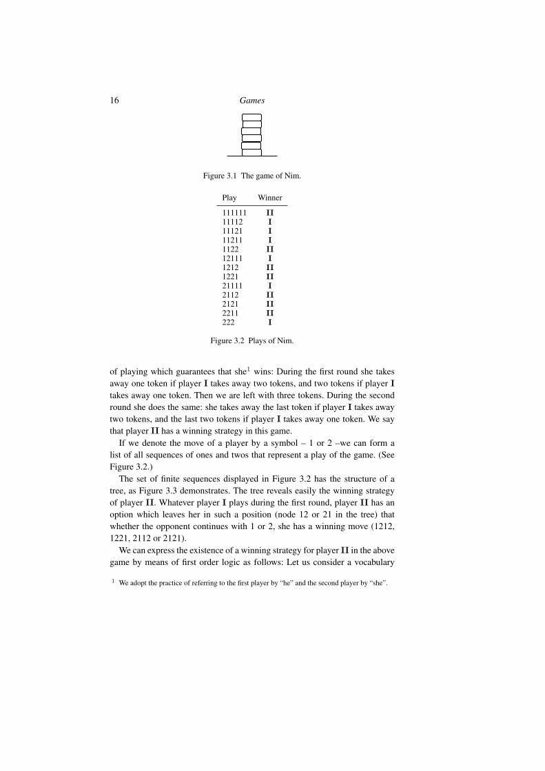
A Preliminary Example: NimIn the game of Nim, if it is simplified to the extreme, there are two players Iand II and a pile of six identical tokens. During each round of the game playerI first removes one or two tokens from the top of the pile and then player IIdoes the same, if any tokens are left. Obviously there can be at most threerounds. The player who removes the last token wins and the other one loses.
The game of Figure 3.1 is an example of a zero-sum two-person game ofperfect information. It is zero-sum because the victory of one player is the lossof the other. It is of perfect information because both players know what theother player has played. A moment’s reflection reveals that player II has a way
16 Games
Figure 3.1 The game of Nim.
Play Winner
111111 II11112 I11121 I11211 I1122 II12111 I1212 II1221 II21111 I2112 II2121 II2211 II222 I
Figure 3.2 Plays of Nim.
of playing which guarantees that she1 wins: During the first round she takesaway one token if player I takes away two tokens, and two tokens if player Itakes away one token. Then we are left with three tokens. During the secondround she does the same: she takes away the last token if player I takes awaytwo tokens, and the last two tokens if player I takes away one token. We saythat player II has a winning strategy in this game.
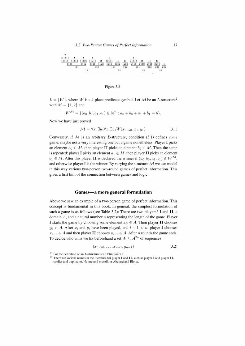
If we denote the move of a player by a symbol – 1 or 2 –we can form alist of all sequences of ones and twos that represent a play of the game. (SeeFigure 3.2.)
The set of finite sequences displayed in Figure 3.2 has the structure of atree, as Figure 3.3 demonstrates. The tree reveals easily the winning strategyof player II. Whatever player I plays during the first round, player II has anoption which leaves her in such a position (node 12 or 21 in the tree) thatwhether the opponent continues with 1 or 2, she has a winning move (1212,1221, 2112 or 2121).
We can express the existence of a winning strategy for player II in the abovegame by means of first order logic as follows: Let us consider a vocabulary
1 We adopt the practice of referring to the first player by “he” and the second player by “she”.
3.2 Two-Person Games of Perfect Information 17
II
11111111111
I
111121111
I
111211112
111
I
112111121
II
1122112
11
I
121111211
II
1212121
II
1221122
121
I
211112111
II
2112211
II
2121212
21
II
2211221
I
22222
2
Figure 3.3
L = {W}, where W is a 4-place predicate symbol. Let M be an L-structure2
with M = {1, 2} and
WM = {(a0, b0, a1, b1) ∈ M4 : a0 + b0 + a1 + b1 = 6}.
Now we have just proved
M |= ∀x0∃y0∀x1∃y1W (x0, y0, x1, y1). (3.1)
Conversely, if M is an arbitrary L-structure, condition (3.1) defines somegame, maybe not a very interesting one but a game nonetheless: Player I picksan element a0 ∈ M , then player II picks an element b0 ∈ M . Then the sameis repeated: player I picks an element a1 ∈ M , then player II picks an elementb1 ∈ M . After this player II is declared the winner if (a0, b0, a1, b1) ∈ WM,and otherwise player I is the winner. By varying the structureMwe can modelin this way various two-person two-round games of perfect information. Thisgives a first hint of the connection between games and logic.
Games—a more general formulation
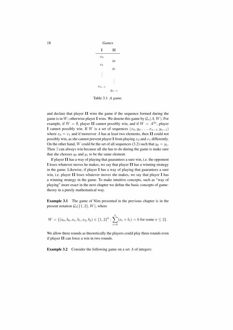
Above we saw an example of a two-person game of perfect information. Thisconcept is fundamental in this book. In general, the simplest formulation ofsuch a game is as follows (see Table 3.2): There are two players3 I and II, adomain A, and a natural number n representing the length of the game. PlayerI starts the game by choosing some element x0 ∈ A. Then player II choosesy0 ∈ A. After xi and yi have been played, and i + 1 < n, player I choosesxi+1 ∈ A and then player II chooses yi+1 ∈ A. After n rounds the game ends.To decide who wins we fix beforehand a set W ⊆ A2n of sequences
(x0, y0, . . . , xn−1, yn−1) (3.2)2 For the definition of an L-structure see Definition 5.1.3 There are various names in the literature for player I and II, such as player I and player II,
spoiler and duplicator, Nature and myself, or Abelard and Eloise.
18 Games
I II
x0
y0
x1
y1
......
xn−1
yn−1
Table 3.1 A game.
and declare that player II wins the game if the sequence formed during thegame is in W ; otherwise player I wins. We denote this game by Gn(A, W ). Forexample, if W = ∅, player II cannot possibly win, and if W = A2n, playerI cannot possibly win. If W is a set of sequences (x0, y0, . . . , xn−1, yn−1)where x0 = x1 and if moreover A has at least two elements, then II could notpossibly win, as she cannot prevent player I from playing x0 and x1 differently.On the other hand, W could be the set of all sequences (3.2) such that y0 = y1.Then ∃ can always win because all she has to do during the game is make surethat she chooses y0 and y1 to be the same element.
If player II has a way of playing that guarantees a sure win, i.e. the opponentI loses whatever moves he makes, we say that player II has a winning strategyin the game. Likewise, if player I has a way of playing that guarantees a surewin, i.e. player II loses whatever moves she makes, we say that player I hasa winning strategy in the game. To make intuitive concepts, such as “way ofplaying” more exact in the next chapter we define the basic concepts of game-theory in a purely mathematical way.
Example 3.1 The game of Nim presented in the previous chapter is in thepresent notation G3({1, 2}, W ), where
W = {(a0, b0, a1, b1, a2, b2) ∈ {1, 2}6 :n�
i=0
(ai + bi) = 6 for some n ≤ 2}.
We allow three rounds as theoretically the players could play three rounds evenif player II can force a win in two rounds.
Example 3.2 Consider the following game on a set A of integers:

Pages deleted for copyright reasons
1
5Models
5.1 Introduction
The concept of a model (or structure) is one of the most fundamental in logic.In brief, while the meaning of logical symbols ∧,∨,∃, ... is always fixed, mod-els give meaning to non-logical symbols such as constant, predicate and func-tion symbols. When we have agreed about the meaning of the logical and non-logical symbols of logic, we can then define the meaning of arbitrary formulas.
Depending on context and preference, models appear in logic in two roles.They can serve the auxiliary role of clarifying logical derivation. For example,one quick way to tell what it means for ϕ to be a logical consequence of ψ isto say that in every model where ψ is true also ϕ is true. It is then an almosttrivial matter to understand why for example ∀x∃yϕ is a logical consequenceof ∃y∀xϕ but ∀y∃xϕ is in general not.
Alternatively models can be the prime objects of investigation and it is thelogical derivation that is in an auxiliary role of throwing light on properties ofmodels. This is manifestly demonstrated by the Completeness Theorem whichsays that any set T of first order sentences has a model unless a contradictioncan be logically derived from T , which entails that the two alternative perspec-tives of models are really equivalent. Since derivations are finite, this impliesthe important Compactness Theorem: If a set of first order sentences is suchthat each of its finite subsets has a model it itself has a model. The Compact-ness Theorem has led to an abundance of non-isomorphic models of first ordertheories, and constitutes the origin of the whole subject of Model Theory. Inthis chapter models are indeed the prime objects of investigation and we in-troduce auxiliary concepts such as the Ehrenfeucht-Fraısse Game that help usunderstand models.
We use the words “model” and “structure” as synonyms. We have a slightpreference for the word “structure” in a context where absolute generality pre-

5.2 Basic Concepts 55
vails and the structures are not assumed to satisfy any particular axioms. Re-spectively, our preference is to call a structure that satisfies some given axiomsa model, so a structure satisfying a theory is called a model of the theory.
5.2 Basic Concepts
A vocabulary is any set L of predicate symbols P,Q, R, . . ., function sym-bols f, g, h, . . ., and constant symbols c, d, e, . . .. Each vocabulary has an arity-function
#L : L → N
which tells the arity of each symbol. Thus if P ∈ L, then P is a #L(P )-arypredicate symbol. If f ∈ L, then f is a #L(f)-ary function symbol. Finally,#L(c) is assumed to be 0 for constants c ∈ L. Predicate or function symbolsof arity 1 are called unary or monadic, and those of arity 2 are called binary.A vocabulary is called unary (or binary) if it contains only unary (respectively,binary) symbols. A vocabulary is called relational if it contains no function orconstant symbols.
Definition 5.1 An L-structure (or L-model) is a pair M = (M, ValM),where M is a non-empty set called the universe (or the domain) of M, andValM is a function defined on L with the following properties:
1. If R ∈ L is a relation symbol and #L(R) = n, then ValM(R) ⊆ Mn.2. If f ∈ L is a function symbol and #L(f) = n, then ValM(f) : Mn → M .3. If c ∈ L is a constant symbol, then ValM(c) ∈ M .
We use Str(L) to denote the class of all L-structures.
We usually shorten ValM(R) to RM, ValM(f) to fM and ValM(c) to cM.If no confusion arises, we use the notation
M = (M,RM1 , . . . , RM
n, fM1 , . . . , fM
m, cM1 , . . . , cM
k)
for an L-structure M, where L = {R1, . . . , Rn, f1, . . . , fm, c1 . . . , ck}.
Example 5.2 Graphs are L-structures for the relational vocabulary L = {E},where E is a predicate symbol with #L(E) = 2. Groups are L-structures forL = {◦}, where ◦ is a binary function symbol. Fields are L-structures forL = {+, ·, 0, 1}, where +, · are binary function symbols and 0, 1 are constantsymbols. Ordered sets (i.e. linear orders) are L-structures for the relationalvocabulary L = {<}, where < is a binary predicate symbol. If L = ∅, anL-structure (M) is a structure with just the universe and no structure in it.
56 Models
If M is a structure and π maps M bijectively onto another set M �, we canuse π to copy the relations, functions and constants of M on M �. In this waywe get a perfect copy M� of M which differs from M only in the respect thatthe underlying elements are different. We then say that M� is an isomorphiccopy of M. For all practical purposes we consider the structures M and M�
as one and the same structure. However, they are not the same structure, justisomorphic. This may sound as if isomorphism was a rather trivial matter, butthis is not true. In many cases it is a highly non-trivial enterprise to investigatewhether two structures are isomorphic or not. In the realm of finite structuresthe question of deciding whether two given structures are isomorphic or not isa famous case of a complexity question which is between P (polynomial time)and NP (non-deterministic polynomial time) and about which we do not knowwhether it is NP-complete. In the light of present knowledge it is conceivablethat this question is strictly between P and NP.
Definition 5.3 L–structures M and M� are isomorphic if there is a bijection
π : M → M �
such that
1. For all a1, . . . , a#L(R) ∈ M :
(a1, . . . , a#L(R)) ∈ RM ⇐⇒ (π(a1), . . . ,π(a#L(R))) ∈ RM�.
2. For all a1, . . . , a#L(f) ∈ M :
fM�(π(a1), . . . ,π(a#L(f))) = π(fM(a1, . . . , a#L(f))).
3. For all c ∈ L: π(cM) = cM�.
In this case we say that π is an isomorphism M→M�, denoted
π : M ∼= M�.
If also M = M�, we say that π an automorphism of M.
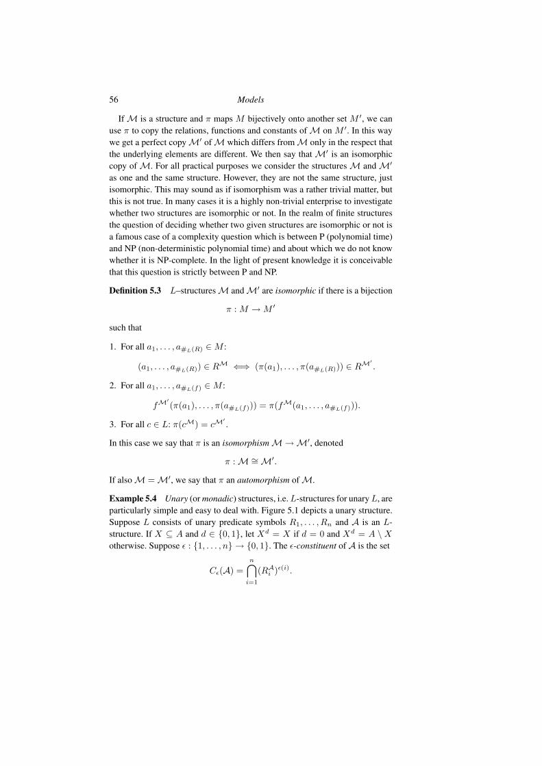
Example 5.4 Unary (or monadic) structures, i.e. L-structures for unary L, areparticularly simple and easy to deal with. Figure 5.1 depicts a unary structure.Suppose L consists of unary predicate symbols R1, . . . , Rn and A is an L-structure. If X ⊆ A and d ∈ {0, 1}, let Xd = X if d = 0 and Xd = A \ Xotherwise. Suppose � : {1, . . . , n}→ {0, 1}. The �-constituent of A is the set
C�(A) =n�
i=1
(RAi
)�(i).
5.2 Basic Concepts 57
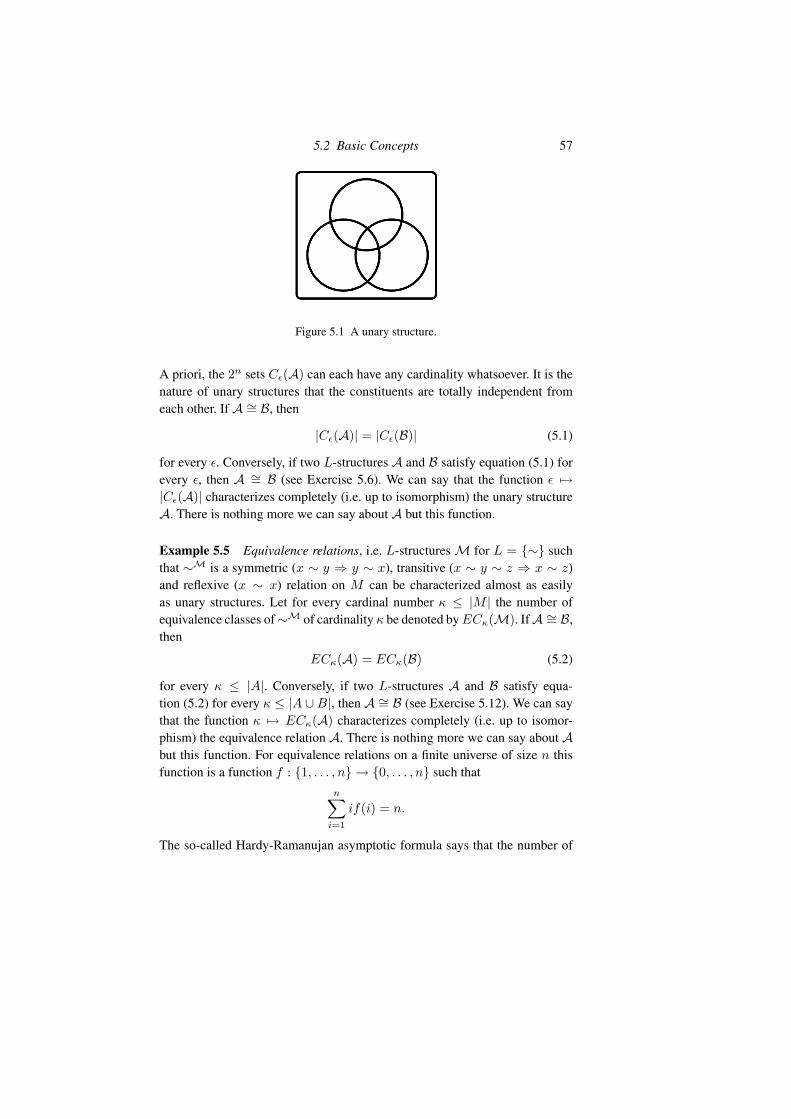
Figure 5.1 A unary structure.
A priori, the 2n sets C�(A) can each have any cardinality whatsoever. It is thenature of unary structures that the constituents are totally independent fromeach other. If A ∼= B, then
|C�(A)| = |C�(B)| (5.1)
for every �. Conversely, if two L-structures A and B satisfy equation (5.1) forevery �, then A ∼= B (see Exercise 5.6). We can say that the function � �→|C�(A)| characterizes completely (i.e. up to isomorphism) the unary structureA. There is nothing more we can say about A but this function.
Example 5.5 Equivalence relations, i.e. L-structures M for L = {∼} suchthat ∼M is a symmetric (x ∼ y ⇒ y ∼ x), transitive (x ∼ y ∼ z ⇒ x ∼ z)and reflexive (x ∼ x) relation on M can be characterized almost as easilyas unary structures. Let for every cardinal number κ ≤ |M | the number ofequivalence classes of∼M of cardinality κ be denoted by ECκ(M). IfA ∼= B,then
ECκ(A) = ECκ(B) (5.2)
for every κ ≤ |A|. Conversely, if two L-structures A and B satisfy equa-tion (5.2) for every κ ≤ |A ∪B|, then A ∼= B (see Exercise 5.12). We can saythat the function κ �→ ECκ(A) characterizes completely (i.e. up to isomor-phism) the equivalence relation A. There is nothing more we can say about Abut this function. For equivalence relations on a finite universe of size n thisfunction is a function f : {1, . . . , n}→ {0, . . . , n} such that
n�
i=1
if(i) = n.
The so-called Hardy-Ramanujan asymptotic formula says that the number of
66 Models
Proof Let P = {f ∈ Part(A,B) : dom(f) is finite}. It turns out that thisstraightforward choice works. Clearly, P �= ∅. Suppose then f ∈ P and a ∈ A.Let us enumerate f as {(a1, b1), . . . , (an, bn)} where a1 < . . . < an. Since fis a partial isomorphism, also b1 < . . . < bn. Now we consider different cases.If a < a1, we choose b < b1 and then f ∪ {(a, b)} ∈ P . If ai < a < ai+1, wechoose b ∈ B so that bi < b < bi+1 and then f ∪ {(a, b)} ∈ P . If an < a, wechoose b > bn and again f ∪{(a, b)} ∈ P . Finally, if a = ai, we let b = bi andthen f ∪ {(a, b)} = f ∈ P . We have proved (5.8). Condition (5.9) is provedsimilarly.
Putting Proposition 5.16 and Proposition 5.17 together yields the famous re-sult of Georg Cantor [Can95]: countable dense linear orders without endpointsare isomorphic. See Exercise 6.29 for a more general result.
5.5 The Ehrenfeucht-Fraısse Game
In Section 4.3 we introduced the Ehrenfeucht-Fraısse Game played on twographs. This game was used to measure to what extent two graphs have sim-ilar properties, especially properties expressible in the first order language ofgraphs limited to a fixed quantifier rank. In this section we extend this game tothe context of arbitrary structures, not just graphs.
Let us recall the basic idea behind the Ehrenfeucht-Fraısse Game. SupposeA and B are L-structures for some relational L. We imagine a situation inwhich two mathematicians argue about whether A and B are isomorphic ornot. The mathematician that we denote by II claims that they are isomorphic,while the other mathematician whom we call I claims the models have anintrinsic structural difference and they cannot possibly be isomorphic.
The matter would be quickly resolved if II was required to show the claimedisomorphism. But the rules of the game are different. The rules are such thatII is required to show only small pieces of the claimed isomorphism.
More exactly, I asks what is the image of an element a1 of A that he choosesat will. Then II is required to respond with some element b1 of B so that
{(a1, b1)} ∈ Part(A,B). (5.10)
Alternatively, I might have chosen an element b1 of B and then II would havebeen required to produce an element a1 of A such that (5.10) holds. The one-element mapping {(a1, b1)} is called the position in the game after the firstmove.
Now the game goes on. Again I asks what is the image of an element a2 of

5.5 The Ehrenfeucht-Fraısse Game 67
Figure 5.5 The Ehrenfeucht-Fraısse Game
A (or alternatively he can ask what is the pre-image of an element b2 of B).Then II produces an element b2 of B (or in the alternative case an element a2
of A). In either case the choice of II has to satisfy
{(a1, b1), (a2, b2)} ∈ Part(A,B). (5.11)
Again, {(a1, b1), (a2, b2)} is called the position after the second move.We continue until the position
{(a1, b1), . . . , (an, bn)} ∈ Part(A,B)
after the nth move has been produced. If II has been able to play all themoves according to the rules she is declared the winner. Let us call this gameEFn(A,B). Figure 5.5 pictures the situation after four moves. If II can winrepeatedly whatever moves I plays, we say that II has a winning strategy.
Example 5.18 Suppose A and B are two L-structures and L = ∅. Thus thestructures A and B consist merely of a universe with no structure on it. Inthis singular case any one-to-one mapping is a partial isomorphism. The onlything player II has to worry about, say in (5.11), is that a1 = a2 if and only ifb1 = b2. Thus II has a winning strategy in EFn(A,B) if A and B both haveat least n elements. So II can have a winning strategy even if A and B havedifferent cardinality and there could be no isomorphism between them for thetrivial reason that there is no bijection. The intuition here is that by playing afinite number of elements, or even ℵ0 many, it is not possible to get hold of thecardinality of the universe if it is infinite.
Example 5.19 Let A be a linear order of length 3 and B a linear order oflength 4. How many moves does I need to beat II? Suppose A = {a1, a2, a3}in increasing order and B = {b1, b2, b3, b4} in increasing order. Clearly, if Iplays at any point the smallest element, also II has to play the smallest elementor face defeat on the next move. Also, if I plays at any point the smallest but

68 Models
one element, also II has to play the smallest but one element or face defeat intwo moves. Now in A the smallest but one element is the same as the largestbut one element, while in B they are different. So if I starts with a2, II has toplay b2 or b3, or else she loses in one move. Suppose she plays b2. Now I playsb3 and II has no good moves left. To obey the rules, she must play a3. That ishow long she can play, for now when I plays b4, II cannot make a legal moveanymore. In fact II has a winning strategy in EF2(A,B) but I has a winningstrategy in EF3(A,B).
We now proceed to a more exact definition of the Ehrenfeucht-Fraısse Game.
Definition 5.20 Suppose L is a vocabulary andM,M� are L-structures suchthat M ∩M � = ∅. The Ehrenfeucht-Fraısse Game EFn(M,M�) is the gameGn(M ∪M �, Wn(M,M�)), where Wn(M,M�) ⊆ (M ∪M �)2n is the set ofp = (x0, y0, . . . , xn−1, yn−1) such that:
(G1) For all i < n: xi ∈ M ⇐⇒ yi ∈ M �.(G2) If we denote
vi =�
xi if xi ∈ Myi if yi ∈ M
v�i=
�xi if xi ∈ M �
yi if yi ∈ M �,
then
fp = {(v0, v�0), . . . , (vn−1, v
�n−1)}
is a partial isomorphism M→M�.
We call vi and v�i
corresponding elements. The infinite game EFω(M,M�)is defined quite similarly, that is, it is the game Gω(M ∪ M �, Wω(M,M�)),where Wω(M,M�) is the set of p = (x0, y0, x1, y1, . . .) such that for alln ∈ N we have (x0, y0, . . . , xn−1, yn−1) ∈ Wn(M,M�).
Note that the game EFω is a closed game.
Proposition 5.21 Suppose L is a vocabulary and A and B are L-structures.the following are equivalent:
1. A �p B.2. II has a winning strategy in EFω(A,B).
Proof Assume A ∩ B = ∅. Let P be first a back-and-forth set for A and B.We define a winning strategy τ = (τi : i < ω) for II. Since P �= ∅ we canfix an element f of P . Condition (5.8) tells us that if a1 ∈ A, then there areb1 ∈ B and g such that
f ∪ {(a1, b1)} ⊆ g ∈ P. (5.12)
5.6 Back-and-Forth Sequences 69
Let τ0(a1) be one such b1. Likewise, if b1 ∈ B, then there are a1 ∈ A such that(5.12) holds and we can let τ0(b1) be some such a1. We have defined τ0(c1)whatever c1 is. To define τ1(c1, c2), let us assume I played c1 = a1 ∈ A. Thus(5.12) holds with b1 = τ0(a1). If c2 = a2 ∈ A we can use (5.8) again to findb2 = τ1(a1, a2) ∈ B and h such that
f ∪ {(a1, b1), (a2, b2)} ⊆ h ∈ P.
The pattern should now be clear. The back-and-forth set P guides II to alwaysfind a valid move. Let us then write the proof in more detail: Suppose we havedefined τi for i < j and we want to define τj . Suppose player I has playedx0, . . . , xj−1 and player II has followed τi during round i < j. During theinductive construction of τi we took care to define also a partial isomorphismfi ∈ P such that {v0, . . . , vi−1} ⊆ dom(fi−1). Now player I plays xj . Byassumption there is fj ∈ P extending fj−1 such that if xj ∈ A, then xj ∈dom(fj) and if xj ∈ B, then xj ∈ rng(fj). We let τj(x0, . . . , xj) = fj(xj)if xj ∈ A and τj(x0, . . . , xj) = f−1
j(xj) otherwise. This ends the construc-
tion of τj . This is a winning strategy because every fp extends to a partialisomorphism M→ N .
For the converse, suppose τ = (τn : n < ω) is a winning strategy of II.Let Q consist of all plays of EFω(A,B) in which player II has used τ . Let Pconsist of all possible fp where p is a position in the game EFω(A,B) with anextension in Q. It is clear that P is non-void and has the properties (5.8) and(5.9).
To prove partial isomorphism of two structures we now have two alternativemethods:
1. Construct a back-and-forth set.2. Show that player II has a winning strategy in EFω.
By Proposition 5.21 these methods are equivalent. In practice one uses thegame as a guide to intuition and then for a formal proof one usually uses aback-and-forth set.
5.6 Back-and-Forth Sequences
Back-and-forth sets and winning strategies of player II in the Ehrenfeucht-Fraısse Game EFω correspond to each other. There is a more refined concept,called back-and-forth sequence, which corresponds to a winning strategy ofplayer II in the finite game EFn.
70 Models
Definition 5.22 A back-and-forth sequence (Pi : i ≤ n) is defined by theconditions
∅ �= Pn ⊆ . . . ⊆ P0 ⊆ Part(A,B). (5.13)
∀f ∈ Pi+1∀a ∈ A∃b ∈ B∃g ∈ Pi(f ∪ {(a, b)} ⊆ g) for i < n. (5.14)
∀f ∈ Pi+1∀b ∈ B∃a ∈ A∃g ∈ Pi(f ∪ {(a, b)} ⊆ g) for i < n. (5.15)
If P is a back-and-forth set, we can get back-and-forth sequences (Pi : i ≤n) of any length by choosing Pi = P for all i ≤ n. But the converse is not true:the sets Pi need by no means be themselves back-and-forth sets. Indeed, pairsof countable models may have long back-and-forth sequences without havingany back-and-forth sets. Let us write
A �n
pB
if there is a back-and-forth sequence of length n for A and B.
Lemma 5.23 The relation �n
pis an equivalence relation on Str(L).
Proof Exactly as Lemma 5.15.
Example 5.24 We use (N + N, <) to denote the linear order obtained byputting two copies of (N, <) one after the other. (The ordinal of this order isω + ω.) Now (N, <) �2
p(N + N, <), for we may take
P2 = {∅}.P1 = {{(a, b)} : 0 < a ∈ N, 0 < b ∈ N + N} ∪ {(0, 0)} ∪ P2.
P0 = {{(a0, b0), (a1, b1)} : a0 < a1 ∈ N, b0 < b1 ∈ N + N} ∪ P1.
Note that (N, <) ��3p
(N + N, <).
Proposition 5.25 Suppose A and B are discrete linear orders (i.e. every el-ement with a successor has an immediate successor and every element witha predecessor has an immediate predecessor) with no endpoints, and n ∈ N.Then A �n
pB.
Proof Let Pi consist of f ∈ Part(A,B) with the following property: f ={(a0, b0), . . . , (an−i−1, bn−i−1)} where
a0 ≤ . . . ≤ an−i−1,
b0 ≤ . . . ≤ bn−i−1,
and for all 0 ≤ j < n − i − 1 if |(aj , aj+1)| < 2i or |(bj , bj+1)| < 2i, then|(aj , aj+1)| = |(bj , bj+1)|.

Pages deleted for copyright reasons
1

76 Models
5.37 Show that there is a complete separable metric space (Polish space)M = (M,d, R, <R) and a non-complete separable metric space M� =(M �, d�, R, <R) such that M �p M�.
5.38 Suppose A and B are structures of the same relational vocabulary L andA ∩B = ∅. The disjoint sum of A and B is the L-structure
(A ∪B, (RA ∪RB)R∈L).
Show that partial isomorphism is preserved by disjoint sums of models.5.39 Suppose A and B are structures of the same vocabulary L. The direct
product of A and B is the L-structure
(A×B, (RA ×RB)R∈L,
(((a0, b0)..., (an, bn)) �→ (fA(a0, ..., an), fB(b0, ..., bn)))f∈L,
((cA, cB))c∈L).
Show that partial isomorphism is preserved by direct products of models.5.40 Show that if two structures are partially isomorphic, then they are po-
tentially isomorphic2 i.e. there is a forcing extension in which they areisomorphic. Conversely, show that if two structures are potentially iso-morphic, then they are partially isomorphic.
5.41 Consider EF2(M,N ), where M = (R × {0}, f), f(x, 0) = (x2, 0)and N = (R× {1}, g), g(x, 1) = (x3, 1). Player I can win even withoutlooking at the moves of II. How?
5.42 Consider EFω(M,N ), where M = (R × {0}, f), f(x, 0) = (x3, 0)and N = (R × {1}, g), g(x, 1) = (x5, 1). After a few moves player Iresigns. Can you explain why?
5.43 Consider EF2(M,N ), where M = (Z, {(a, b) : a−b = 10}) and N =(Q, {(a, b) : a− b = 2/3}). Suppose we are in position (−8,−1/4) (i.e.x0 = −8 and y0 = −1/4). Then I plays x1 = 11/12. What would be agood move for II?
5.44 Consider EFω(M,N ), where M and N are as in the previous exercise.Player I resigns before the game even starts. Can you explain why?
5.45 Suppose M and N are disjoint sets with 10 elements each. Let c ∈ Mand d ∈ N . Who has a winning strategy in EFω(M,N ) in the followingcases:
1. M = (M, {(a, b, c) : a = b}),N = (N, {(a, b, d) : a = b}),2. M = (M, {(a, b, e) : a = b}),N = (N, {(a, b, e) : b = e}).
2 Some authors use the term potential isomorphism for partial isomorphism.

Pages deleted for copyright reasons
1

6First Order Logic
6.1 Introduction
We have already discussed the first order language of graphs. We now definethe basic concepts of a more general first order language, denoted FO, onewhich applies to any vocabulary, not just the vocabulary of graphs. First or-der logic fits the Strategic Balance of Logic better than any other logic. It isarguably the most important of all logics. It has enough power to express inter-esting and important concept and facts, and still it is weak and flexible enoughto permit powerful constructions as demonstrated e.g. by the Model ExistenceTheorem below.
6.2 Basic Concepts
Suppose L is a vocabulary. The logical symbols of the first order language (orlogic) of the vocabulary L are ≈,¬,∧,∨,∀,∃, (, ), x0, x1, . . .. Terms are de-fined as follows: Constant symbols c ∈ L are L-terms. Variables x0, x1, ... areL-terms. If f ∈ L, #(f) = n and t1, . . . , tn are L-terms, then so is ft1 . . . tn.L-equations are of the form ≈tt� where t and t� are L-terms. L-atomic formu-las are either L-equations or of the form Rt1 . . . tn, where R ∈ L, #(R) = nand t1, ..., tn are L-terms. A basic formula is an atomic formula or the negationof an atomic formula. L-formulas are of the form
≈tt�
Rt1 . . . tn¬ϕ(ϕ ∧ ψ), (ϕ ∨ ψ)∀xnϕ,∃xnϕ

6.2 Basic Concepts 81
where t, t�, t1, ..., tn are L-terms, R ∈ L with #(R) = n, and ϕ and ψ areL-formulas.
Definition 6.1 An assignment for a set M is any function s with dom(s) a setof variables and rng(s) ⊆M. The value tM(s) of an L-term t inM under theassignment s is defined as follows: cM(s) = ValM(c), xM
n(s) = s(xn) and
(ft1 . . . tn)M(s) = ValM(f)(tM1 (s), . . . , tMn
(s)). The truth of L-formulas inM under s is defined as follows:
M �s Rt1 . . . tn iff (tM1 (s), . . . , tMn
(s)) ∈ ValM(R)M �s ≈t1t2 iff tM1 (s) = tM2 (s)M �s ¬ϕ iff M �s ϕM �s (ϕ ∧ ψ) iff M �s ϕ and M �s ψM �s (ϕ ∨ ψ) iff M �s ϕ or M �s ψM �s ∀xnϕ iff M �s[a/xn] ϕ for all a ∈MM �s ∃xnϕ iff M �s[a/xn] ϕ for some a ∈M,
where s[a/xn](y) =�
a if y = xn
s(y) otherwise.
We assume the reader is familiar with such basic concepts as free variable,sentence, substitution of terms for variables etc. A standard property of firstorder (or any other) logic is that M |=s ϕ depends only on M and the valuesof s on the variables that are free in ϕ. A sentence is a formula ϕ without freevariables. Then M |= ϕ means M |=∅ ϕ. In this case we say that ϕ is true inM.
Convention: If ϕ is an L-formula with the free variables x1, . . . , xn, we in-dicate this by writing ϕ as ϕ(x1, . . . , xn). If M is an L-structure and s is anassignment for M such that M |=s ϕ, we write M |= ϕ(a1, . . . , an), whereai = s(xi) for i = 1, . . . , n.
Definition 6.2 The quantifier rank of a formula ϕ, denoted qr(ϕ), is definedas follows: qr(≈tt�) = qr(Rt1 . . . tn) = 0, qr(¬ϕ) = qr(ϕ), qr((ϕ ∧ ψ)) =qr((ϕ ∨ ψ)) = max{qr(ϕ), qr(ψ)}, qr(∃xϕ) = qr(∀xϕ) = qr(ϕ) + 1. Aformula ϕ is quantifier free if qr(ϕ) = 0.
The quantifier rank is a measure of the longest sequence of “nested” quan-tifiers. In the first three of the following formulas the quantifiers ∀xn and ∃xn
are nested but in the last unnested:
∀x0(P (x0) ∨ ∃x1R(x0, x1)) (6.1)
∃x0(P (x0) ∧ ∀x1R(x0, x1)) (6.2)
∀x0(P (x0) ∨ ∃x1Q(x1)) (6.3)
82 First Order Logic
(∀x0P (x0) ∨ ∃x1Q(x1)) (6.4)
Note that formula (6.3) of quantifier rank 2 is logically equivalent to the for-mula (6.4) which has quantifier rank 1. So the nesting can sometimes be elim-inated. In formulas (6.1) and (6.2) nesting cannot be so eliminated.
Proposition 6.3 Suppose L is a finite vocabulary without function symbols.For every n and for every set {x1, . . . , xn} of variables, there are only finitelymany logically non-equivalent first order L-formulas of quantifier rank < nwith the free variables {x1, . . . , xn}.
Proof The proof is exactly like that of Proposition 4.15.
Note that Proposition 6.3 is not true for infinite vocabularies, as there wouldbe infinitely many logically non-equivalent atomic formulas, and also not truefor vocabularies with function symbols, as there would be infinitely many log-ically non-equivalent equations obtained by iterating the function symbols.
6.3 Characterizing Elementary Equivalence
We now show that the concept of a back-and-forth sequence provides an alter-native characterization of elementary equivalence
A ≡ B i.e. ∀ϕ ∈ FO(A |= ϕ ⇐⇒ B |= ϕ).
This is the original motivation for the concepts of a back-and-forth set, back-and-forth sequence and Ehrenfeucht-Fraısse Game. To this end, let
A ≡n B
mean that A and B satisfy the same sentences of FO of quantifier rank ≤ n.We now prove an important leg of the Strategic Balance of Logic, namely
the marriage of truth and separation:
Proposition 6.4 Suppose L is an arbitrary vocabulary. Suppose A and B areL-structures and n ∈ N. Consider the conditions:
(i) A ≡n B.(ii) A�
L� �n
pB�
L� for all finite L� ⊆ L.
We have always (ii) → (i) and if L has no function symbols, then (ii) ↔ (i).
Proof (ii)→(i). If A �≡n B, then there is a sentence ϕ of quantifier rank ≤ nsuch that A |= ϕ and B �|= ϕ. Since ϕ has only finitely many symbols, there

6.3 Characterizing Elementary Equivalence 83
is a finite L� ⊆ L such that A�L� �≡n B�
L� . Suppose (Pi : i ≤ n) is a back-and-forth sequence for A�
L� and B�L� . We use induction on i ≤ n to prove the
following
Claim If f ∈ Pi and a1, . . . , ak ∈ dom(f), then
(A�L� , a1, . . . , ak) ≡i (B�
L� , fa1, . . . , fak).
If i = 0, the claim follows from P0 ⊆ Part(A�L� ,B�
L�). Suppose thenf ∈ Pi+1 and a1, . . . , ak ∈ dom(f). Let ϕ(x0, x1, . . . , xk) be an L�-formulaof FO of quantifier rank ≤ i such that
A�L� |= ∃x0ϕ(x0, a1, . . . , ak).
Let a ∈ A so that A�L� |= ϕ(a, a1, . . . , ak) and g ∈ Pi such that a ∈ dom(g)
and f ⊆ g. By the induction hypothesis, B�L� |= ϕ(ga, ga1, . . . , gak). Hence
B�L� |= ∃x0ϕ(x0, fa1, . . . , fak).
The claim is proved. Putting i = n and using the assumption Pn �= ∅, gives acontradiction with A�
L� �≡n B�L� .
(i) → (ii). Assume L has no function symbols. Fix L� ⊆ L finite. Let Pi
consist of f : A → B such that dom(f) = {a0, . . . , an−i−1} and
(A�L� , a0, . . . , an−i−1) ≡i (B�
L� , fa0, . . . , fan−i−1).
We show that (Pi : i ≤ n) is a back-and-forth sequence for A�L� and B�
L� .By (i), ∅ ∈ Pn so Pn �= ∅. Suppose f ∈ Pi, i > 0, as above, and a ∈ A.By Proposition 6.3 there are only finitely many pairwise non-equivalent L�-formulas of quantifier rank i− 1 of the form ϕ(x, x0, . . . , xn−i−1) in FO. Letthem be ϕj(x, x0, . . . , xn−i−1), j ∈ J . Let
J0 = {j ∈ J : A�L� |= ϕj(a, a0, . . . , an−i−1)}.
Let
ψ(x, x0, . . . , xn−i−1) =�
j∈J0
ϕj(x, x0, . . . , xn−i−1) ∧
�
j∈J\J0
¬ϕj(x, x0, . . . , xn−i−1).
Now A�L� |= ∃xψ(x, a0, . . . , an−i−1), so as we have assumed f ∈ Pi, we
have B�L� |= ∃xψ(x, fa0, . . . , fan−i−1). Thus there is some b ∈ B with
B�L� |= ψ(b, fa0, . . . , fan−i−1). Now f ∪ {(a, b)} ∈ Pi−1. The other condi-
tion (5.15) is proved similarly.
84 First Order Logic
The above Proposition is the standard method for proving models elemen-tary equivalent in FO. For example, Proposition 6.4 and Example 5.26 togethergive (Z, <) ≡ (Z + Z, <). The exercises give more examples of partially iso-morphic pairs—and hence elementary equivalent—structures. The restrictionon function symbols can be circumvented by first using quantifiers to elim-inate nesting of function symbols and then replacing the unnested equationsf(x1, ..., xn−1) = xn by new predicate symbols R(x1, ..., xn).
Let Str(L) denote the class of all L-structures. We can draw the followingimportant conclusion from Proposition 6.4 (see Figure 6.1):
Corollary Suppose L is a vocabulary without function symbols. Then for alln ∈ N the equivalence relation
A ≡n B
divides Str(L) into finitely many equivalence classes Cn
i, i = 1, . . . ,mn, such
that for each Cn
ithere is a sentence ϕn
iof FO with the properties:
1. For all L-structures A: A ∈ Cn
i⇐⇒ A |= ϕn
i.
2. If ϕ is an L-sentence of quantifier rank ≤ n, then there are i1, . . . , ik suchthat |= ϕ ↔ (ϕn
i1∨ . . . ∨ ϕn
ik)
Proof Let ϕn
ibe the conjunction of all the finitely many L-sentences of quan-
tifier rank ≤ n that are true in some (every) model in Cn
i(to make the con-
junction finite we do not repeat logically equivalent formulas). For the secondclaim, let ϕn
i1, . . . ,ϕn
ikbe the finite set of all L-sentences of quantifier rank
≤ n that are consistent with ϕ. If now A |= ϕ, and A ∈ Cn
i, then A |= ϕn
i.
On the other hand, if A |= ϕn
iand there is B |= ϕn
isuch that B |= ϕ, then
A ≡n B, whence A |= ϕ.
We can actually read from the proof of Proposition 6.4 a more accuratedescription for the sentences ϕi. This leads to the theory of so-called Scottformulas (see Section 7.4).
Theorem 6.5 Suppose K is a class of L-structures. Then the following areequivalent (see Figure 6.2):
1. K is FO-definable, i.e. there is an L-sentence ϕ of FO such that for allLstructures M we have M ∈ K ⇐⇒ M |= ϕ.
2. There is n ∈ N such that K is closed under �n
p.
As in the case of graphs, Theorem 6.5 can be used to demonstrate that certainproperties of models are not definable in FO:

6.3 Characterizing Elementary Equivalence 85
Figure 6.1 First order definable model class K
Figure 6.2 Not first order definable model class K
Example 6.6 Let L = ∅. The following properties of L-structures M are notexpressible in FO:
1. M is infinite.2. M is finite and even.
In both cases it is easy to find, for each n ∈ N, two models Mn and Nn suchthat Mn �n
pNn, M has the property, but N does not.
Example 6.7 Let L = {P} be a unary vocabulary. The following propertiesof L-structures (M,A) are not expressible in FO:
1. |A| = |M |.2. |A| = |M \A|.
86 First Order Logic
3. |A| ≤ |M \A|.
This is demonstrated by the models (N, {1, . . . , n}), (N, N \ {1, . . . , n}) and({1, . . . , 2n}, {1, . . . , n}).
Example 6.8 Let L = {<} be a binary vocabulary. The following propertiesof L-structures M = (M,<) are not expressible in FO:
1. M ∼= (Z, <).2. All closed intervals of M are finite.3. Every bounded subset of M has a supremum.
This is demonstrated in the first two cases by the models Mn = (Z, <) andNn = (Z + Z, <) (see Example 5.26), and in the third case by the partiallyisomorphic models: M = (R, <) and N = (R \ {0}, <).
6.4 The Lowenheim-Skolem Theorem
In this section we show that if a first order sentence ϕ is true in a structure M,it is true in a countable substructure of M, and even more, there are countablesubstructures of M in a sense “everywhere” satisfying ϕ. To make this state-ment precise we introduce a new game due to D. Kueker [Kue77] called thecub game.
Definition 6.9 Suppose A is an arbitrary set. Pω(A) is defined as the set ofall countable subsets of A.
The set Pω(A) is an auxiliary concept useful for the general investigation ofcountable substructures of a model with universe A. One should note that if Ais infinite, the setPω(A) is uncountable1. For example, |Pω(N)| = |R|. The setPω(A) is closed under intersections and countable unions but not necessarilyunder complements, so it is a (distributive) lattice under the partial order ⊆,but not a Boolean algebra. The sets in Pω(A) cover the set A entirely, but sodo many proper subsets of Pω(A) such as the set of all singletons in Pω(A)and the set of all finite sets in Pω(A).
Definition 6.10 Suppose A is an arbitrary set and C a subset of Pω(A). Thecub game of C is the game Gcub(C) = Gω(A, W ), where W consists of se-quences (a1, a2, . . .) with the property that {a1, a2, . . .} ∈ C.
1 Its cardinality is |A|ω .
6.4 The Lowenheim-Skolem Theorem 87
I II
a0
a1
a2
a3
......
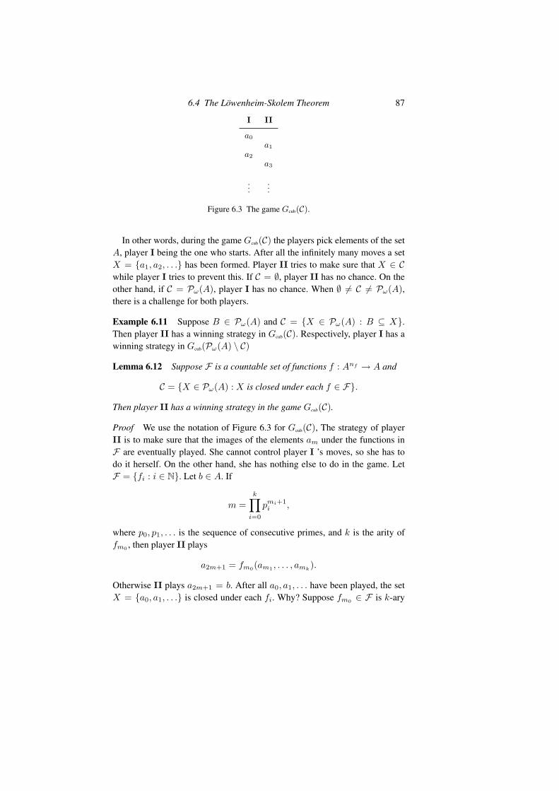
Figure 6.3 The game Gcub(C).
In other words, during the game Gcub(C) the players pick elements of the setA, player I being the one who starts. After all the infinitely many moves a setX = {a1, a2, . . .} has been formed. Player II tries to make sure that X ∈ Cwhile player I tries to prevent this. If C = ∅, player II has no chance. On theother hand, if C = Pω(A), player I has no chance. When ∅ �= C �= Pω(A),there is a challenge for both players.
Example 6.11 Suppose B ∈ Pω(A) and C = {X ∈ Pω(A) : B ⊆ X}.Then player II has a winning strategy in Gcub(C). Respectively, player I has awinning strategy in Gcub(Pω(A) \ C)
Lemma 6.12 Suppose F is a countable set of functions f : Anf → A and
C = {X ∈ Pω(A) : X is closed under each f ∈ F}.
Then player II has a winning strategy in the game Gcub(C).
Proof We use the notation of Figure 6.3 for Gcub(C), The strategy of playerII is to make sure that the images of the elements am under the functions inF are eventually played. She cannot control player I ’s moves, so she has todo it herself. On the other hand, she has nothing else to do in the game. LetF = {fi : i ∈ N}. Let b ∈ A. If
m =k�
i=0
pmi+1i
,
where p0, p1, . . . is the sequence of consecutive primes, and k is the arity offm0 , then player II plays
a2m+1 = fm0(am1 , . . . , amk).
Otherwise II plays a2m+1 = b. After all a0, a1, . . . have been played, the setX = {a0, a1, . . .} is closed under each fi. Why? Suppose fm0 ∈ F is k-ary
88 First Order Logic
I II
a00
b00
a01
b01
......
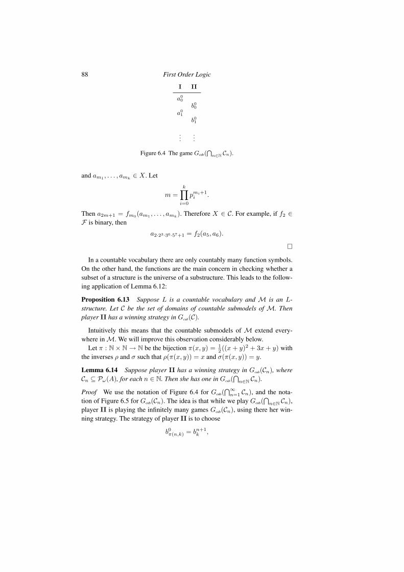
Figure 6.4 The game Gcub(T
n∈N Cn).
and am1 , . . . , amk ∈ X . Let
m =k�
i=0
pmi+1i
.
Then a2m+1 = fm0(am1 , . . . , amk). Therefore X ∈ C. For example, if f2 ∈F is binary, then
a2·23·36·57+1 = f2(a5, a6).
In a countable vocabulary there are only countably many function symbols.On the other hand, the functions are the main concern in checking whether asubset of a structure is the universe of a substructure. This leads to the follow-ing application of Lemma 6.12:
Proposition 6.13 Suppose L is a countable vocabulary and M is an L-structure. Let C be the set of domains of countable submodels of M. Thenplayer II has a winning strategy in Gcub(C).
Intuitively this means that the countable submodels of M extend every-where in M. We will improve this observation considerably below.
Let π : N× N → N be the bijection π(x, y) = 12 ((x + y)2 + 3x + y) with
the inverses ρ and σ such that ρ(π(x, y)) = x and σ(π(x, y)) = y.
Lemma 6.14 Suppose player II has a winning strategy in Gcub(Cn), whereCn ⊆ Pω(A), for each n ∈ N. Then she has one in Gcub(
�n∈N Cn).
Proof We use the notation of Figure 6.4 for Gcub(�∞
n=1 Cn), and the nota-tion of Figure 6.5 for Gcub(Cn). The idea is that while we play Gcub(
�n∈N Cn),
player II is playing the infinitely many games Gcub(Cn), using there her win-ning strategy. The strategy of player II is to choose
b0π(n,k) = bn+1
k,
6.4 The Lowenheim-Skolem Theorem 89
I II
an0
bn0
an1
bn1
......
Figure 6.5 The game Gcub(Cn).
I II
a0
b0
a1
b1
......
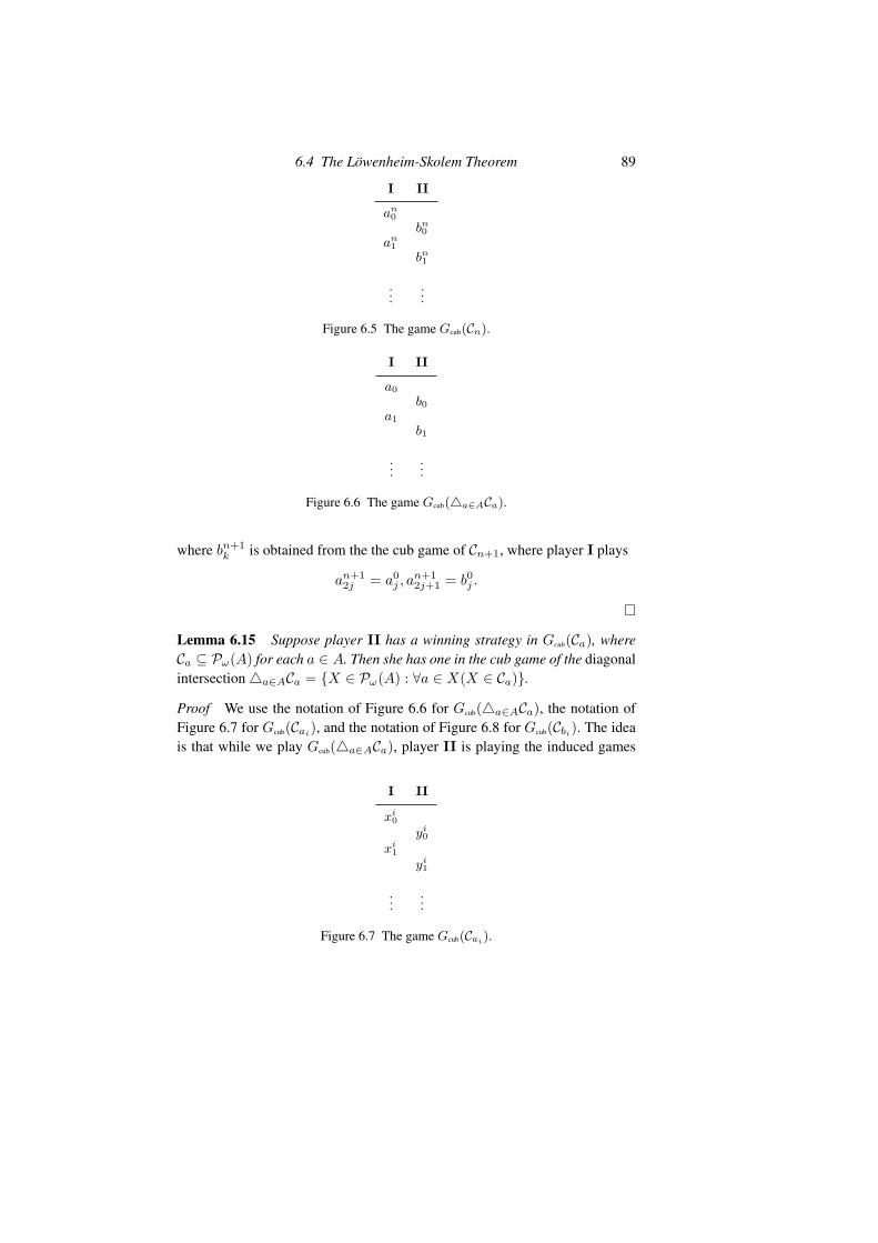
Figure 6.6 The game Gcub(�a∈ACa).
where bn+1k
is obtained from the the cub game of Cn+1, where player I plays
an+12j
= a0j, an+1
2j+1 = b0j.
Lemma 6.15 Suppose player II has a winning strategy in Gcub(Ca), whereCa ⊆ Pω(A) for each a ∈ A. Then she has one in the cub game of the diagonalintersection �a∈ACa = {X ∈ Pω(A) : ∀a ∈ X(X ∈ Ca)}.
Proof We use the notation of Figure 6.6 for Gcub(�a∈ACa), the notation ofFigure 6.7 for Gcub(Cai), and the notation of Figure 6.8 for Gcub(Cbi). The ideais that while we play Gcub(�a∈ACa), player II is playing the induced games
I II
xi0
yi0
xi1
yi1
......
Figure 6.7 The game Gcub(Cai).
90 First Order Logic
I II
ui0
vi0
ui1
vi1
......
Figure 6.8 The game Gcub(Cbi).
I II
a0
b0
a1
b1
......
Figure 6.9 The game Gcub(�a∈ACa).
Gcub(Cai) and Gcub(Cbi), using there her winning strategy. The strategy of playerII is to choose
b2π(n,k) = yn
k, b2π(n,k)+1 = vn
k,
where bn+1k
is obtained from Gcub(Cai), where player I plays
xi+12j
= aj , xi+12j+1 = bj ,
and from Gcub(Cbi), where player I plays
ui+12j
= aj , ui+12j+1 = bj .
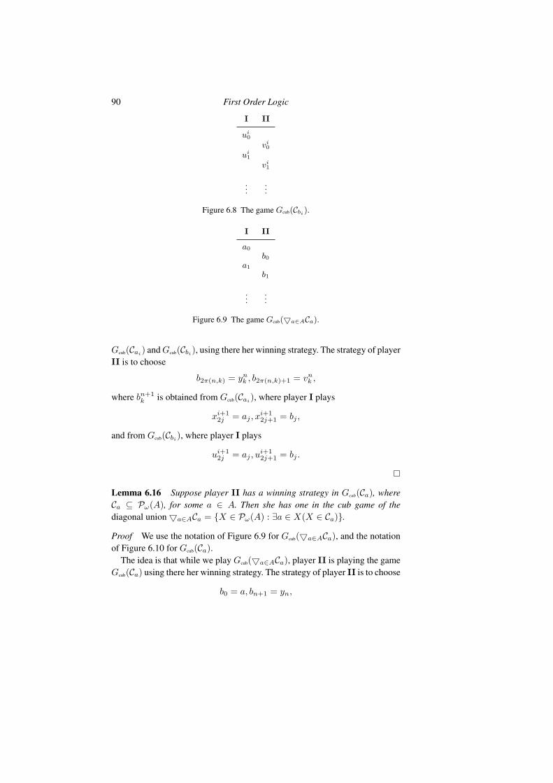
Lemma 6.16 Suppose player II has a winning strategy in Gcub(Ca), whereCa ⊆ Pω(A), for some a ∈ A. Then she has one in the cub game of thediagonal union �a∈ACa = {X ∈ Pω(A) : ∃a ∈ X(X ∈ Ca)}.
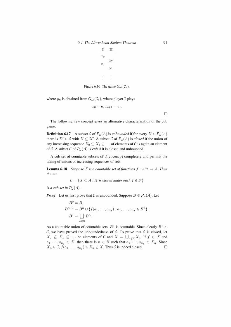
Proof We use the notation of Figure 6.9 for Gcub(�a∈ACa), and the notationof Figure 6.10 for Gcub(Ca).
The idea is that while we play Gcub(�a∈ACa), player II is playing the gameGcub(Ca) using there her winning strategy. The strategy of player II is to choose
b0 = a, bn+1 = yn,
6.4 The Lowenheim-Skolem Theorem 91
I II
x0
y0
x1
y1
......
Figure 6.10 The game Gcub(Ca).
where yn is obtained from Gcub(Ca), where player I plays
x0 = a, xi+1 = ai.
The following new concept gives an alternative characterization of the cubgame:
Definition 6.17 A subset C of Pω(A) is unbounded if for every X ∈ Pω(A)there is X � ∈ C with X ⊆ X �. A subset C of Pω(A) is closed if the union ofany increasing sequence X0 ⊆ X1 ⊆ . . . of elements of C is again an elementof C. A subset C of Pω(A) is cub if it is closed and unbounded.
A cub set of countable subsets of A covers A completely and permits thetaking of unions of increasing sequences of sets.
Lemma 6.18 Suppose F is a countable set of functions f : Anf → A. Thenthe set
C = {X ⊆ A : X is closed under each f ∈ F}
is a cub set in Pω(A).
Proof Let us first prove that C is unbounded. Suppose B ∈ Pω(A). Let
B0 = B,
Bn+1 = Bn ∪ {f(a1, . . . , anf ) : a1, . . . , anf ∈ Bn},
B∗ =�
n∈NBn.
As a countable union of countable sets, B∗ is countable. Since clearly B∗ ∈C, we have proved the unboundedness of C. To prove that C is closed, letX0 ⊆ X1 ⊆ . . . be elements of C and X =
�n∈N Xn. If f ∈ F and
a1, . . . , anf ∈ X , then there is n ∈ N such that a1, . . . , anf ∈ Xn. SinceXn ∈ C, f(a1, . . . , anf ) ∈ Xn ⊆ X . Thus C is indeed closed.
92 First Order Logic
Now we can prove a characterization of the cub game in terms of cub sets:
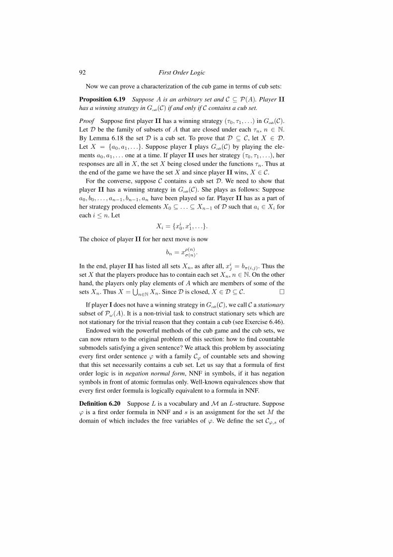
Proposition 6.19 Suppose A is an arbitrary set and C ⊆ P(A). Player IIhas a winning strategy in Gcub(C) if and only if C contains a cub set.
Proof Suppose first player II has a winning strategy (τ0, τ1, . . .) in Gcub(C).Let D be the family of subsets of A that are closed under each τn, n ∈ N.By Lemma 6.18 the set D is a cub set. To prove that D ⊆ C, let X ∈ D.Let X = {a0, a1, . . .}. Suppose player I plays Gcub(C) by playing the ele-ments a0, a1, . . . one at a time. If player II uses her strategy (τ0, τ1, . . .), herresponses are all in X , the set X being closed under the functions τn. Thus atthe end of the game we have the set X and since player II wins, X ∈ C.
For the converse, suppose C contains a cub set D. We need to show thatplayer II has a winning strategy in Gcub(C). She plays as follows: Supposea0, b0, . . . , an−1, bn−1, an have been played so far. Player II has as a part ofher strategy produced elements X0 ⊆ . . . ⊆ Xn−1 of D such that ai ∈ Xi foreach i ≤ n. Let
Xi = {xi
0, xi
1, . . .}.
The choice of player II for her next move is now
bn = xρ(n)σ(n).
In the end, player II has listed all sets Xn, as after all, xi
j= bπ(i,j). Thus the
set X that the players produce has to contain each set Xn, n ∈ N. On the otherhand, the players only play elements of A which are members of some of thesets Xn. Thus X =
�n∈N Xn. Since D is closed, X ∈ D ⊆ C.
If player I does not have a winning strategy in Gcub(C), we call C a stationarysubset of Pω(A). It is a non-trivial task to construct stationary sets which arenot stationary for the trivial reason that they contain a cub (see Exercise 6.46).
Endowed with the powerful methods of the cub game and the cub sets, wecan now return to the original problem of this section: how to find countablesubmodels satisfying a given sentence? We attack this problem by associatingevery first order sentence ϕ with a family Cϕ of countable sets and showingthat this set necessarily contains a cub set. Let us say that a formula of firstorder logic is in negation normal form, NNF in symbols, if it has negationsymbols in front of atomic formulas only. Well-known equivalences show thatevery first order formula is logically equivalent to a formula in NNF.
Definition 6.20 Suppose L is a vocabulary and M an L-structure. Supposeϕ is a first order formula in NNF and s is an assignment for the set M thedomain of which includes the free variables of ϕ. We define the set Cϕ,s of
6.4 The Lowenheim-Skolem Theorem 93
countable subsets of M as follows: If ϕ is atomic, Cϕ,s contains as an elementthe domain A of a countable submodel A of M such that rng(s) ⊆ A and:
• If ϕ is ≈tt�, then tA(s) = t�A(s).• If ϕ is ¬≈tt�, then tA(s) �= t�A(s).• If ϕ is Rt1 . . . tn, then (tA1 (s), . . . , tnA(s)) ∈ RA.• If ϕ is ¬Rt1 . . . tn, then (tA1 (s), . . . , tnA(s)) /∈ RA.
For non-basic ϕ we define
• Cϕ∧ψ,s = Cϕ,s ∩ Cψ,s.• Cϕ∨ψ,s = Cϕ,s ∪ Cψ,s.• C∃xϕ,s = �a∈MCϕ,s(a/x).• C∀xϕ,s = �a∈MCϕ,s[a/x].
If ϕ is a sentence, we denote Cϕ,s by Cϕ. If ϕ is not in NNF, we define Cϕ,s
and Cϕ by first translating ϕ into a logically equivalent NNF formula.
The sets Cϕ were defined with the following fact in mind:
Proposition 6.21 Suppose A is an L-structure such that A ∈ Cϕ,s. ThenA |=s ϕ.
Proof This is trivial for atomic ϕ. The induction step is clear for ϕ ∧ ψ andϕ ∨ ψ. Suppose A ∈ C∃xϕ,s. Thus A ∈ �a∈MCϕ,s[a/x]. By the definition ofdiagonal union A ∈ Cϕ,s[a/x] for some a ∈ A. By the induction hypothesis,A |=s[a/x] ϕ for some a ∈ A. Thus A |=s ∃xϕ. Finally, suppose A ∈ C∀xϕ,s.Thus A ∈ �a∈MCϕ,s[a/x]. By the definition of diagonal intersection A ∈Cϕ,s[a/x] for all a ∈ A. By the induction hypothesis, A |=s[a/x] ϕ for alla ∈ A. Thus A |=s ∀xϕ.
Proposition 6.22 Suppose L is countable and M an L-structure such thatM |= ϕ. Then player II has a winning strategy in Gcub(Cϕ).
Proof We use induction on ϕ to prove that if M |=s ϕ, then II has awinning strategy in Gcub(Cϕ). For atomic formulas the claim follows fromProposition 6.13. The induction step is clear for ϕ ∨ ψ. The induction stepfor ϕ ∧ ψ follows from Lemma 6.14. The induction step for ∀xϕ and ∃xϕfollows from Lemma 6.16. Finally, the induction step for ∀xϕ follows fromLemma 6.15.
Theorem 6.23 (Lowenheim-Skolem Theorem) Suppose L is a countable vo-cabulary and T is a set of L-sentences. If M is a model of T , then player IIhas a winning strategy in
Gcub({X ∈ Pω(M) : [X]M |= T}).
94 First Order Logic
In particular, for every countable X ⊆ M there is a countable submodel N ofM such that X ⊆ N and N |= T .
Proof Let T = {ϕ0, ϕ1, . . .}. By Proposition 6.22 player II has a winningstrategy in Gcub(Cϕn). By Lemma 6.14, player II has a winning strategy inGcub(
�∞n=0 Cϕn). If X ∈
�∞n=0 Cϕn , then [X]M |= T .
6.5 The Semantic Game
The truth of a first order sentence in a structure can be defined by means of asimple game called the Semantic Game. We examine this game in detail andgive some applications of it.
Definition 6.24 Suppose L is a vocabulary, M is an L-structure, ϕ∗ is anL-formula and s∗ is an assignment for M . The game SGsym(M, ϕ∗) is definedas follows. In the beginning player II holds (ϕ∗, s∗). The rules of the game areas follows:
1. If ϕ is atomic, and s satisfies it in M, then the player who holds (ϕ, s) winsthe game, otherwise the other player wins.
2. If ϕ = ¬ψ, then the player who holds (ϕ, s), gives (ψ, s) to the other player.3. If ϕ = ψ ∧ θ, then the player who holds (ϕ, s), switches to hold (ψ, s) or
(θ, s), and the other player decides which.4. If ϕ = ψ ∨ θ, then the player who holds (ϕ, s), switches to hold (ψ, s) or
(θ, s), and can himself or herself decide which.5. If ϕ = ∀xψ, then the player who holds (ϕ, s), switches to hold (ψ, s[a/x])
for some a, and the other player decides for which.6. If ϕ = ∃xψ, then the player who holds (ϕ, s), switches to hold (ψ, s[a/x])
for some a, and can himself or herself decide for which.
As was pointed out in Section 4.2, M |=s ϕ if and only if player II has awinning strategy in the above game, starting with (ϕ, s). Why? If M |=s ϕ,then the winning strategy of player II is to play so that if she holds (ϕ�, s�),then M |=s� ϕ�, and if player I holds (ϕ�, s�), then M �|=s� ϕ�.
For practical purposes it is useful to consider a simpler game which pre-supposes that the formula is in negation normal form. In this game, as in theEhrenfeucht-Fraısse Game, player I assumes the role of a doubter and playerII the role of confirmer. This makes the game easier to use than the full gameSGsym(M, ϕ).

6.5 The Semantic Game 95
I IIx0 y0x1 y1
......
Figure 6.11 The game Gω(W ).
xn yn Explanation Rule
(ϕ, ∅) I enquires about ϕ ∈ T .
(ϕ, ∅) II confirms. Axiom rule
(ϕi, s) I tests a played (ϕ0 ∧ ϕ1, s)by choosing i ∈ {0, 1}.
(ϕi, s) II confirms. ∧-rule
(ϕ0 ∨ ϕ1, s) I enquires abouta played disjunction.
(ϕi, s) II makes a choice of i ∈ {0, 1}. ∨-rule
(ϕ, s[a/x]) I tests a played (∀xϕ, s)by choosing a ∈ M .
(ϕ, s[a/x]) II confirms. ∀-rule
(∃xϕ, s) I enquires abouta played existential statement.
(ϕ, s[a/x]) II makes a choice of a ∈ M . ∃-rule
Figure 6.12 The game SG(M, T ).
Definition 6.25 The Semantic Game SG(M, T ) of the set T of L-sentencesin NNF is the game (see Figure 6.11) Gω(W ), where W consists of sequences(x0, y0, x1, y1, . . .) where player II has followed the rules of Figure 6.12 andif player II plays the pair (ϕ, s), where ϕ is a basic formula, then M |=s ϕ.
In the game SG(M, T ) player II claims that every sentence of T is true in
96 First Order Logic
M. Player I doubts this and challenges player II. He may doubt whether acertain ϕ ∈ T is true in M, so he plays x0 = (ϕ, ∅). In this round, as in someother rounds too, player II just confirms and plays the same pair as player I.This may seem odd and unnecessary, but it is for book-keeping purposes only.Player I in a sense gathers a finite set of formulas confirmed by player II andtries to end up with a basic formula which cannot be true.
Theorem 6.26 Suppose L is a vocabulary, T is a set of L-sentences, and Mis an L-structure. Then the following are equivalent:
1. M |= T .2. Player II has a winning strategy in SG(M, T ).
Proof Suppose M |= T . The winning strategy of player II in SG(M, T ) isto maintain the condition M |=si ψi for all yi = (ψi, si), i ∈ N, played byher. It is easy to see that this is possible. On the other hand, suppose M �|= T ,say M �|= ϕ, where ϕ ∈ T . The winning strategy of player I in SG(M, T ) isto start with x0 = (ϕ, ∅), and then maintain the condition M �|=si ψi for allyi = (ψi, si), i ∈ N, played by II:
1. If yi = (ψi, si), where ψi is basic, then player I has won the game, becauseM �|=si ψi.
2. If yi = (ψi, si), where ψi = θ0 ∧ θ1, then player I can use the assumptionM �|=si ψi to find k < 2 such that M �|=si θk. Then he plays xi+1 =(θk, si).
3. If yi = (ψi, si), where ψi = θ0 ∨ θ1, then player I knows from the as-sumption M �|=si ψi that whether II plays (θk, si) for k = 0 or k = 1, thecondition M �|=si θk still holds. So player I can play xi+1 = (ψi, si) andkeep his winning criterion in force.
4. If yi = (ψi, si), where ψi = ∀xϕ, then player I can use the assumptionM �|=si ψi to find a ∈ M such that M �|=si[a/x] ϕ. Then he plays xi+1 =(ϕ, si[a/x]).
5. If yi = (ψi, si), where ψi = ∃xϕ, then player I knows from the assumptionM �|=si ψi that whatever (ϕ, si[a/x]) player II chooses to play, the condi-tion M �|=si[a/x] ϕ still holds. So player I can play (∃xϕ, si) and keep hiswinning criterion in force.
Example 6.27 Let L = {f} and M = (N, fM), where f(n) = n + 1. Let
ϕ = ∀x∃y≈fxy.

6.5 The Semantic Game 97
I II Rule
(∀x∃y≈fxy, ∅)(∀x∃y≈fxy, ∅) Axiom rule
(∃y≈fxy, {(x, 25)})(∃y≈fxy, {(x, 25)}) ∀-rule
(∃y≈fxy, {(x, 25)})(≈fxy, {(x, 25), (y, 26)}) ∃-rule
......
Figure 6.13 Player II has a winning strategy in SG(M, {ϕ}).
I II Rule
(∀x∃y≈fyx, ∅)(∀x∃y≈fyx, ∅) Axiom rule
(∃y≈fyx, {(x, 0)})(∃y≈fyx, {(x, 0)}) ∀-rule
(∃y≈fyx, {(x, 0)})(≈fyx, {(x, 0), (y, 2)}) ∃-rule(II has no good move)
Figure 6.14 Player I wins the game SG(M, {ψ}).
Clearly, M |= ϕ. Thus player II has, by Theorem 6.26, a winning strategy inthe game SG(M, {ϕ}). Figure 6.13 shows how the game might proceed.On the other hand, suppose
ψ = ∀x∃y≈fyx.
Clearly, M �|= ϕ. Thus player I has, by Theorem 6.26 and Theorem 3.12, awinning strategy in the game SG(M, {ϕ}). Figure 6.14 shows how the gamemight proceed:
Example 6.28 Let M be the graph of Figure 6.15.and
ϕ = ∀x(∃y¬xEy ∧ ∃yxEy).
Clearly, M |= ϕ. Thus player II has, by Theorem 6.26, a winning strategy inthe game SG(M, {ϕ}). Figure 6.16 shows how the game might proceed.On the other hand, suppose
ψ = ∃x(∀y¬xEy ∨ ∀yxEy).
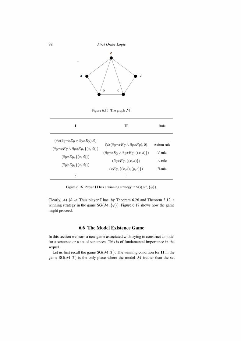
98 First Order Logic
Figure 6.15 The graph M.
I II Rule
(∀x(∃y¬xEy ∧ ∃yxEy), ∅)(∀x(∃y¬xEy ∧ ∃yxEy), ∅) Axiom rule
(∃y¬xEy ∧ ∃yxEy, {(x, d)})(∃y¬xEy ∧ ∃yxEy, {(x, d)}) ∀-rule
(∃yxEy, {(x, d)})(∃yxEy, {(x, d)}) ∧-rule
(∃yxEy, {(x, d)})(xEy, {(x, d), (y, c)}) ∃-rule
......
Figure 6.16 Player II has a winning strategy in SG(M, {ϕ}).
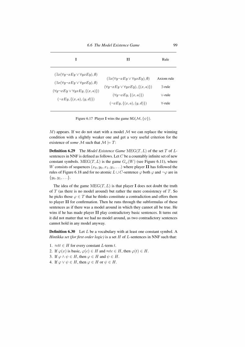
Clearly, M �|= ϕ. Thus player I has, by Theorem 6.26 and Theorem 3.12, awinning strategy in the game SG(M, {ϕ}). Figure 6.17 shows how the gamemight proceed.
6.6 The Model Existence Game
In this section we learn a new game associated with trying to construct a modelfor a sentence or a set of sentences. This is of fundamental importance in thesequel.
Let us first recall the game SG(M, T ): The winning condition for II in thegame SG(M, T ) is the only place where the model M (rather than the set
6.6 The Model Existence Game 99
I II Rule
(∃x(∀y¬xEy ∨ ∀yxEy), ∅)(∃x(∀y¬xEy ∨ ∀yxEy), ∅) Axiom rule
(∃x(∀y¬xEy ∨ ∀yxEy), ∅)(∀y¬xEy ∨ ∀yxEy), {(x, a)}) ∃-rule
(∀y¬xEy ∨ ∀yxEy, {(x, a)})(∀y¬xEy, {(x, a)}) ∨-rule
(¬xEy, {(x, a), (y, d)})(¬xEy, {(x, a), (y, d)}) ∀-rule
Figure 6.17 Player I wins the game SG(M, {ψ}).
M ) appears. If we do not start with a model M we can replace the winningcondition with a slightly weaker one and get a very useful criterion for theexistence of some M such that M |= T :
Definition 6.29 The Model Existence Game MEG(T,L) of the set T of L-sentences in NNF is defined as follows. Let C be a countably infinite set of newconstant symbols. MEG(T,L) is the game Gω(W ) (see Figure 6.11), whereW consists of sequences (x0, y0, x1, y1, . . .) where player II has followed therules of Figure 6.18 and for no atomic L∪C-sentence ϕ both ϕ and ¬ϕ are in{y0, y1, . . .}.
The idea of the game MEG(T,L) is that player I does not doubt the truthof T (as there is no model around) but rather the mere consistency of T . Sohe picks those ϕ ∈ T that he thinks constitute a contradiction and offers themto player II for confirmation. Then he runs through the subformulas of thesesentences as if there was a model around in which they cannot all be true. Hewins if he has made player II play contradictory basic sentences. It turns outit did not matter that we had no model around, as two contradictory sentencescannot hold in any model anyway.
Definition 6.30 Let L be a vocabulary with at least one constant symbol. AHintikka set (for first order logic) is a set H of L-sentences in NNF such that:
1. ≈tt ∈ H for every constant L-term t.2. If ϕ(x) is basic, ϕ(c) ∈ H and ≈tc ∈ H , then ϕ(t) ∈ H .3. If ϕ ∧ ψ ∈ H , then ϕ ∈ H and ψ ∈ H .4. If ϕ ∨ ψ ∈ H , then ϕ ∈ H or ψ ∈ H .

100 First Order Logic
xn yn Explanation
ϕ I enquires about ϕ ∈ T .
ϕ II confirms.
≈tt I enquires about an equation.
≈tt II confirms.
ϕ(t�) I chooses played ϕ(t) and ≈tt� with ϕ basicand enquires about substituting t� for t in ϕ.
ϕ(t�) II confirms.
ϕi I tests a played ϕ0 ∧ ϕ1 by choosing i ∈ {0, 1}.
ϕi II confirms.
ϕ0 ∨ ϕ1 I enquires about a played disjunction.
ϕi II makes a choice of i ∈ {0, 1}
ϕ(c) I tests a played ∀xϕ(x) by choosing c ∈ C.
ϕ(c) II confirms.
∃xϕ(x) I enquires about a played existential statement.
ϕ(c) II makes a choice of c ∈ C
t I enquires about a constant L ∪ C-term t.
≈ct II makes a choice of c ∈ C
Figure 6.18 The game MEG(T, L).
5. If ∀xϕ(x) ∈ H , then ϕ(c) ∈ H for all c ∈ L
6. If ∃xϕ(x) ∈ H , then ϕ(c) ∈ H for some c ∈ L.7. For every constant L-term t there is c ∈ L such that ≈ct ∈ H .8. There is no atomic sentence ϕ such that ϕ ∈ H and ¬ϕ ∈ H .
6.6 The Model Existence Game 101
Lemma 6.31 Suppose L is a vocabulary and T is a set of L-sentences. If Thas a model, then T can be extended to a Hintikka set.
Proof Let us assume M |= T . Let L� ⊇ L such that L� has a constantsymbol ca /∈ L for each a ∈ M . Let M∗ be an expansion of M obtained byinterpreting ca by a for each a ∈ M . Let H be the set of all L�-sentences truein M. It is easy to verify that H is a Hintikka set.
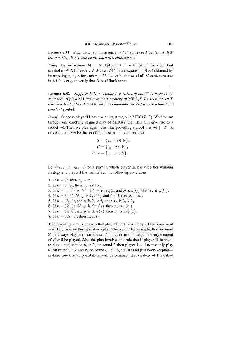
Lemma 6.32 Suppose L is a countable vocabulary and T is a set of L-sentences. If player II has a winning strategy in MEG(T,L), then the set Tcan be extended to a Hintikka set in a countable vocabulary extending L byconstant symbols.
Proof Suppose player II has a winning strategy in MEG(T,L). We first runthrough one carefully planned play of MEG(T,L). This will give rise to amodel M. Then we play again, this time providing a proof that M |= T . Tothis end, let Trm be the set of all constant L ∪ C-terms. Let
T = {ϕn : n ∈ N},C = {cn : n ∈ N},
T rm = {tn : n ∈ N}.
Let (x0, y0, x1, y1, . . .) be a play in which player II has used her winningstrategy and player I has maintained the following conditions:
1. If n = 3i, then xn = ϕi.2. If n = 2 · 3i, then xn is ≈cici.3. If n = 4 · 3i · 5j · 7k · 11l, yi is ≈tjtk, and yl is ϕ(tj), then xn is ϕ(tk).4. If n = 8 · 3i · 5j , yi is θ0 ∧ θ1, and j < 2, then xn is θj .5. If n = 16 · 3i, and yi is θ0 ∨ θ1, then xn is θ0 ∨ θ1.6. If n = 32 · 3i · 5j , yi is ∀xϕ(x), then xn is ϕ(cj).7. If n = 64 · 3i, and yi is ∃xϕ(x), then xn is ∃xϕ(x).8. If n = 128 · 3i, then xn is ti.
The idea of these conditions is that player I challenges player II in a maximalway. To guarantee this he makes a plan. The plan is, for example, that on round3i he always plays ϕi from the set T . Thus in an infinite game every elementof T will be played. Also the plan involves the rule that if player II happensto play a conjunction θ0 ∧ θ1 on round i, then player I will necessarily playθ0 on round 8 · 3i and θ1 on round 8 · 3i · 5, etc. It is all just book-keeping—making sure that all possibilities will be scanned. This strategy of I is called
102 First Order Logic
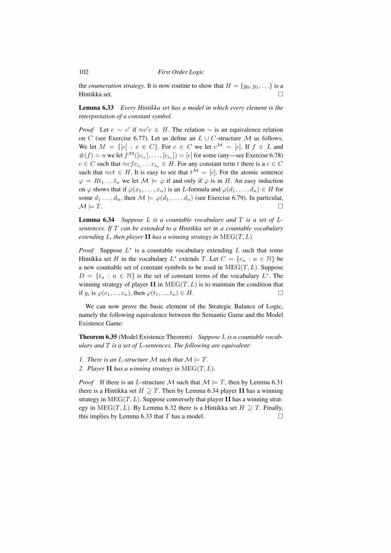
the enumeration strategy. It is now routine to show that H = {y0, y1, . . .} is aHintikka set.
Lemma 6.33 Every Hintikka set has a model in which every element is theinterpretation of a constant symbol.
Proof Let c ∼ c� if ≈c�c ∈ H . The relation ∼ is an equivalence relationon C (see Exercise 6.77). Let us define an L ∪ C-structure M as follows.We let M = {[c] : c ∈ C}. For c ∈ C we let cM = [c]. If f ∈ L and#(f) = n we let fM([ci1 ], . . . , [cin ]) = [c] for some (any—see Exercise 6.78)c ∈ C such that ≈cfci1 . . . cin ∈ H . For any constant term t there is a c ∈ Csuch that ≈ct ∈ H . It is easy to see that tM = [c]. For the atomic sentenceϕ = Rt1 . . . tn we let M |= ϕ if and only if ϕ is in H . An easy inductionon ϕ shows that if ϕ(x1, . . . , xn) is an L-formula and ϕ(d1, . . . , dn) ∈ H forsome d1 . . . , dn, then M |= ϕ(d1, . . . , dn) (see Exercise 6.79). In particular,M |= T .
Lemma 6.34 Suppose L is a countable vocabulary and T is a set of L-sentences. If T can be extended to a Hintikka set in a countable vocabularyextending L, then player II has a winning strategy in MEG(T,L)
Proof Suppose L∗ is a countable vocabulary extending L such that someHintikka set H in the vocabulary L∗ extends T . Let C = {cn : n ∈ N} bea new countable set of constant symbols to be used in MEG(T,L). SupposeD = {tn : n ∈ N} is the set of constant terms of the vocabulary L∗. Thewinning strategy of player II in MEG(T,L) is to maintain the condition thatif yi is ϕ(c1, ..., cn), then ϕ(t1, ..., tn) ∈ H .
We can now prove the basic element of the Strategic Balance of Logic,namely the following equivalence between the Semantic Game and the ModelExistence Game:
Theorem 6.35 (Model Existence Theorem) Suppose L is a countable vocab-ulary and T is a set of L-sentences. The following are equivalent:
1. There is an L-structure M such that M |= T .2. Player II has a winning strategy in MEG(T,L).
Proof If there is an L-structure M such that M |= T , then by Lemma 6.31there is a Hintikka set H ⊇ T . Then by Lemma 6.34 player II has a winningstrategy in MEG(T,L). Suppose conversely that player II has a winning strat-egy in MEG(T,L). By Lemma 6.32 there is a Hintikka set H ⊇ T . Finally,this implies by Lemma 6.33 that T has a model.

Pages deleted for copyright reasons
1
132 First Order Logic
set Cn ⊆ Dn. Let C =�Cn and show that C can have only one element,
which contradicts the fact that C is cub.)6.47 Use the previous exercise to conclude that CUBA is not an ultrafilter (i.e.
a maximal filter) if A is infinite.6.48 Show that the set NSA of sets C ⊆ Pω(A) which are non-stationary is a
σ-ideal (i.e. (1) If D ∈ NSA and C ⊆ D ⊆ Pω(A), then C ∈ NSA. (2)If Dn ∈ NSA for all n ∈ N, then
�n∈N Dn ∈ NSA). In fact, NSA is a
normal ideal (i.e. if Da ∈ NSA for all a ∈ A, then �a∈ADa ∈ NSA).6.49 Show that if a sentence is true in a stationary set of countable submodels
of a model then it is true in the model itself. More exactly: Let L bea countable vocabulary, M an L-model and ϕ an L-sentence. Suppose{X ∈ Pω(M) : [X]M |= ϕ} is stationary. Show that M |= ϕ.
6.50 In this and the following exercises we develop the theory of cub andstationary subsets of a regular cardinal κ > ω. A set C ⊆ κ is closed if itcontains every non-zero limit ordinal δ < κ such that C∩δ is unboundedin δ, and unbounded if it is unbounded as a subset of κ. We call C ⊆ κa closed unbounded (cub) set if C is both closed and unbounded. Showthat the following sets are cub
(i) κ(ii) {α < κ : α is a limit ordinal}(iii) {α < κ : α = ωβ for some β}(iv) {α < κ : if β < α and γ < α, then β + γ < α}(v) {α < κ : if α = β · γ, then α = β or α = γ}.
6.51 Show that he following sets are not cub:
(i) ∅(ii) {α < ω1 : α = β + 1 for some β}(iii) {α < ω1 : α = ωβ + ω for some β}(iv) {α < ω2 : cf(α) = ω}.
6.52 Show that a set C contains a cub subset of ω1 if and only if player IIwins the game Gω(WC), where
WC = {(x0, x1, x2, . . .) : supn
xn ∈ C}.
6.53 A filter F on M is λ-closed if Aα ∈ F for α < β, where β < λ, implies�α
Aα ∈ F . A filter F on κ is normal if Aα ∈ F for α < κ implies�αAα ∈ F , where
�αAα = {α < κ : α ∈ Aβ for all β < α}.
Note that normality implies κ-closure. Show that if κ > ω is regular,

Exercises 133
then the set F of subsets of κ that contain a cub set is a proper normalfilter on κ. The filter F is called the cub-filter on κ.
6.54 A subset of κ which meets every cub set is called stationary. Equiva-lently, a subset S of κ is stationary if its complement is not in the cub-filter. A set which is not stationary, is non-stationary. Show that all setsin the cub-filter are stationary. Show that
{α < ω2 : cof(α) = ω}
is a stationary set which is not in the cub-filter on ω2.6.55 (Fodor’s lemma, second formulation) Suppose κ > ω is a regular car-
dinal. If S ⊆ κ is stationary and f : S → κ satisfies f(α) < α for allα ∈ S, then there is a stationary S� ⊆ S such that f is constant on S�.(Hint: For each α < κ let Sα = {β < κ : f(β) = α}. Show that one ofthe sets Sα has to be stationary. )
6.56 Suppose κ is a regular cardinal > ω. Show that there is a bistationaryset S ⊆ κ (i.e. both S and κ \ S are stationary). (Hint: Note that S ={α < κ : cf(α) = ω} is always stationary. For α ∈ S let δα : ω → α bestrictly increasing with sup
nδα(n) = α. By the previous exercise there
is for each n < ω a stationary An ⊆ S such that the regressive functionfn(α) = δα(n) is constant δn on An. Argue that some κ \ An must bestationary.)
6.57 Suppose κ is a regular cardinal > ω. Show that κ =�
α<κSα where the
sets Sα are disjoint stationary sets. (Hint: Proceed as in Exercise 6.56.Find n < ω such that for all β < κ the set Sβ = {α < κ : δα(n) ≥ β}is stationary. Find stationary S�
β⊆ Sβ such that δα(n) is constant for
α ∈ S�β
. Argue that there are κ different sets S�β
.)6.58 Show that S ⊆ ω1 is bistationary if and only if the game Gω(WS) is
non-determined.6.59 Suppose κ is regular > ω. Show that S ⊆ κ is stationary if and only if
every regressive f : S → κ is constant on an unbounded set.6.60 Prove that C ⊆ ω1 is in the cub filter if and only if almost all countable
subsets of ω1 have their sup in C.6.61 Suppose S ⊆ ω1 is stationary. Show that for all α < ω1 there is a closed
subset of S of order-type≥ α. (Hint: Prove a stronger claim by inductionon α.)
6.62 Decide first which of the following are true and then show how the win-ner should play the game SG(M, T ):
1. (R, <, 0) |= ∃x∀y(y < x ∨ 0 < y)2. (N, <) |= ∀x∀y(¬y < x ∨ ∀z(z < y ∨ ¬z < x)).

134 First Order Logic
6.63 Prove directly that if II has a winning strategy in SG(M, T ) and M �p
N , then II has a winning strategy in SG(N , T ).6.64 The Existential Semantic Game SG∃(M, T ) differs from SG(M, T )
only in that the ∀-rule is omitted. Show that if II has a winning strat-egy in SG∃(M, T ) and M ⊆ N , then II has a winning strategy inSG∃(N , T ).
6.65 A formula in NNF is existential if it contains no universal quantifiers.(Then it is logically equivalent to one of the form ∃x1 . . .∃xnϕ, where ϕis quantifier free.) Show that if L is countable and T is a set of existentialL-sentences, thenM |= T if and only if player II has a winning strategyin the game SG∃(M, T ).
6.66 The Universal-Existential Semantic Game SG∀∃(M, T ) differs from thegame SG(M, T ) only in that player I has to make all applications of the∀-rule before all applications of the ∃-rule. Show that if M0 ⊆ M1 ⊆. . . and II has a winning strategy in each SG∀∃(Mn, T ), then II has awinning strategy in SG∀∃(∪∞n=0Mn, T ).
6.67 A formula in NNF is universal-existential if it is of the form
∀y1 . . .∀yn∃x1 . . .∃xmϕ,
where ϕ is quantifier free. Show that if L is countable and T is a set ofuniversal-existential L-sentences, then M |= T if and only if player IIhas a winning strategy in the game SG∀∃(M, T ).
6.68 The Positive Semantic Game SGpos(M, T ) differs from SG(M, T ) onlyin that the winning condition “If player II plays the pair (ϕ, s), whereϕ is basic, then M |=s ϕ” is weakened to “If player II plays the pair(ϕ, s), where ϕ is atomic, then M |=s ϕ”. Suppose M and N are L-structures. A surjection h : M → N is a homomorphism M → Nif
M |= ϕ(a1, . . . , an) ⇒ N |= ϕ(f(a1), . . . , f(an))
for all atomic L-formulas ϕ and all a1, . . . , an ∈ M . Show that if IIhas a winning strategy in SGpos(M, T ) and h : M → N is a surjectivehomomorphism, then II has a winning strategy in SGpos(N , T ).
6.69 A formula in NNF is positive if it contains no negations. Show that if Lis countable and T is a set of positive L-sentences, then M |= T if andonly if player II has a winning strategy in the game SGpos(M, T ).
6.70 The game MEG(T,L) is played with
T = {Pc,¬Qfc,∀x0(¬Px0 ∨Qx0),∀x0(¬Px0 ∨ Pfx0)}.
The game starts as in Figure 6.22. How does I play now and win?
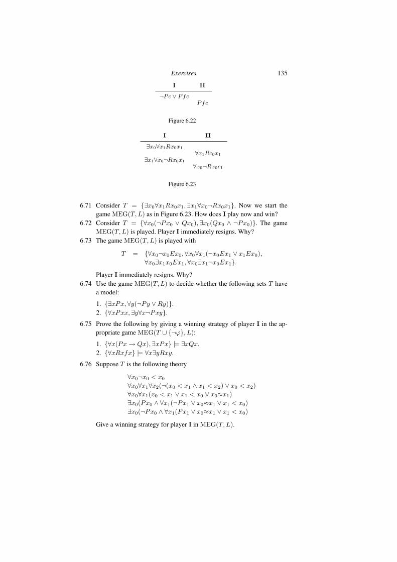
Exercises 135
I II
¬Pc ∨ PfcPfc
Figure 6.22
I II
∃x0∀x1Rx0x1
∀x1Rc0x1
∃x1∀x0¬Rx0x1
∀x0¬Rx0c1
Figure 6.23
6.71 Consider T = {∃x0∀x1Rx0x1,∃x1∀x0¬Rx0x1}. Now we start thegame MEG(T,L) as in Figure 6.23. How does I play now and win?
6.72 Consider T = {∀x0(¬Px0 ∨ Qx0),∃x0(Qx0 ∧ ¬Px0)}. The gameMEG(T,L) is played. Player I immediately resigns. Why?
6.73 The game MEG(T,L) is played with
T = {∀x0¬x0Ex0,∀x0∀x1(¬x0Ex1 ∨ x1Ex0),∀x0∃x1x0Ex1,∀x0∃x1¬x0Ex1}.
Player I immediately resigns. Why?6.74 Use the game MEG(T,L) to decide whether the following sets T have
a model:
1. {∃xPx,∀y(¬Py ∨Ry)}.2. {∀xPxx,∃y∀x¬Pxy}.
6.75 Prove the following by giving a winning strategy of player I in the ap-propriate game MEG(T ∪ {¬ϕ}, L):
1. {∀x(Px → Qx),∃xPx} |= ∃xQx.2. {∀xRxfx} |= ∀x∃yRxy.
6.76 Suppose T is the following theory
∀x0¬x0 < x0
∀x0∀x1∀x2(¬(x0 < x1 ∧ x1 < x2) ∨ x0 < x2)∀x0∀x1(x0 < x1 ∨ x1 < x0 ∨ x0≈x1)∃x0(Px0 ∧ ∀x1(¬Px1 ∨ x0≈x1 ∨ x1 < x0)∃x0(¬Px0 ∧ ∀x1(Px1 ∨ x0≈x1 ∨ x1 < x0)
Give a winning strategy for player I in MEG(T,L).

Pages deleted for copyright reasons
1
7Infinitary Logic
7.1 Introduction
As the name indicates, infinitary logic has infinite formulas. The oldest use ofinfinitary formulas is the elimination of quantifiers in number theory:
∃xϕ(x) ↔�
n∈Nϕ(n)
∀xϕ(x) ↔�
n∈Nϕ(n).
Here we leave behind logic as a study of sentences humans can write downon paper. Infinitary formulas are merely mathematical objects used to studyproperties of structures and proofs. It turns out that games are particularly suit-able for the study of infinitary logic. In a sense games replace the use of theCompactness Theorem which fails badly in infinitary logic.
7.2 Preliminary Examples
The games we have encountered so far have had a fixed length, which hasbeen either a natural number or ω (an infinite game). Now we introduce agame which is “dynamic” in the sense that it is possible for player I to changethe length of the game during the game. He may first claim he can win in fivemoves, but seeing what the first move of II is, he may decide he needs tenmoves. In these games player I is not allowed to declare he will need infinitelymany moves, although we shall study such games, too, later.
Before giving a rigorous definition of the Dynamic Ehrenfeucht-Fraısse gamewe discuss some simple versions of it.

7.2 Preliminary Examples 141
Definition 7.1 (Preliminary) Suppose M,M� are L-structures such that L isa relational vocabulary and M ∩M � = ∅. The Dynamic Ehrenfeucht-Fraıssegame, denoted EFDω(M,M�) is defined as follows: First player I chooses anatural number n and then the game EFn(M,M�) is played.
Note that EFDω(M,M�) is not a game of length ω. Player II has a winningstrategy in EFDω(M,M�) if she has one in each EFn(M,M�). On the otherhand, player I has a winning strategy in EFDω(M,M�) if he can envisage anumber n so that he has a winning strategy in EFn(M,M�).
Example 7.2 If M and M� are L-structures such that M is finite and M �
is infinite, then player I has a winning strategy in EFDω(M,M�). Suppose|M | = n. Player I has a winning strategy in EFn+1(M,M�). He first playsall n elements of M and then any unplayed element of M �. Player II is out ofgood moves, and loses the game.
Example 7.3 IfM andM� are equivalence relations such thatM has finitelymany equivalence classes and M� infinitely many, then player I has a win-ning strategy in EFDω(M,M�). Suppose the equivalence classes of M are[a1], . . . , [an]. The strategy of I is to play first the elements a1, . . . , an. Thenhe plays an element from M � which is not equivalent to any element played sofar. Player II is at a loss. She has to play an element of M equivalent to one ofa1, . . . , an. She loses.
Definition 7.4 (Preliminary) Suppose n ∈ N. The game EFDω+n(M,M�)is played as follows. First the game EFω(M,M�) is played for n moves. Thenplayer I declares a natural number m and the game EFω(M,M�) is continuedfor m more moves. If II has not lost yet, she has won EFDω+n(M,M�).Otherwise player I has won.
Example 7.5 Suppose G and G� are graphs so that in G every vertex has afinite degree while in G� some vertex has infinite degree. Then player I hasa winning strategy in EFDω+1(G,G�). Suppose a ∈ G � has infinite degree.Player I plays first the element a. Let b ∈ G be the response of player II. Weknow that every element of G has finite degree. Let the degree of b be n. PlayerI declares that we play n+1 more moves. Accordingly, he plays n+1 differentneighbors of a. Player II cannot play n+1 different neighbors of b since b hasdegree n. She loses.
Example 7.6 Suppose G is a connected graph and G� a disconnected graph.Then player I has a winning strategy in EFDω+2(G,G�). Suppose a and b areelements of G � that are not connected by a path. Player I plays first elementsa and b. Suppose the responses of player II are c and d. Since G is connected,
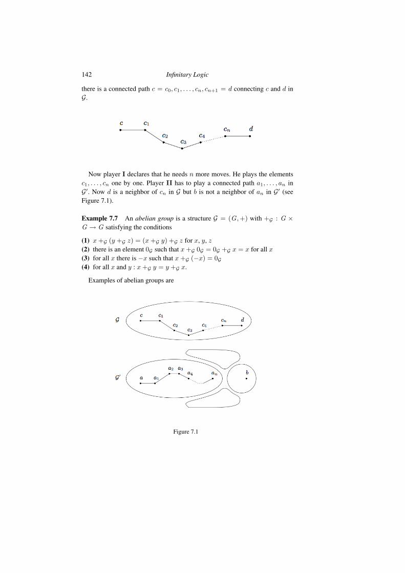
142 Infinitary Logic
there is a connected path c = c0, c1, . . . , cn, cn+1 = d connecting c and d inG.
Now player I declares that he needs n more moves. He plays the elementsc1, . . . , cn one by one. Player II has to play a connected path a1, . . . , an inG�. Now d is a neighbor of cn in G but b is not a neighbor of an in G� (seeFigure 7.1).
Example 7.7 An abelian group is a structure G = (G ,+) with +G : G ×G → G satisfying the conditions
(1) x +G (y +G z) = (x +G y) +G z for x, y, z(2) there is an element 0G such that x +G 0G = 0G +G x = x for all x(3) for all x there is −x such that x +G (−x) = 0G(4) for all x and y : x +G y = y +G x.
Examples of abelian groups are
Figure 7.1

Pages deleted for copyright reasons
1

8Model Theory of Infinitary Logic
8.1 Introduction
The model theory of Lω1ω is dominated by the Model Existence Theorem. Itmore or less takes the role of the Compactness Theorem which can be right-fully called the cornerstone of model theory of first order logic. The ModelExistence Theorem is used to prove the Craig Interpolation Theorem and theimportant undefinability of the concept of well-order. When we move to thestronger logics Lκ+ω, κ > ω, the Model Existence Theorem in general fails.However, we use a union of chains argument to prove the undefinability ofwell-order. In the final section we introduce game quantifiers. Here we crossthe line to logics in which well-order is definable. Game quantifiers permit anapproximation process which leads to the Covering Theorem, a kind of Inter-polation Theorem.
8.2 Lowenheim-Skolem Theorem for L∞ω
In Section 6.4 we saw that if a first order sentence is true in a model it is true in“almost” every countable approximation of that model. We now extend this toL∞ω but of course with some modification because L∞ω has consistent sen-tences without any countable models. We show that if a sentence ϕ of L∞ω istrue in a structure M, a countable ”approximation” of ϕ is true in a countable”approximation” of M, and even more, there are this kind of approximationsof ϕ and M in a sense “everywhere”. To make this statement precise we em-ploy the cub game introduced in Definition 6.10. We say
...X... for almost all X ∈ Pω(A)
178 Model Theory of Infinitary Logic
if
player II has a winning strategy in Gcub(Pω(A)).
Recall the following facts:
1. If X0 ∈ Pω(A), then X0 ⊆ X for almost all X ∈ Pω(A).2. If X ∈ C for almost all X ∈ Pω(A) and C ⊆ C�, then X ∈ C� for almost
all X ∈ Pω(A).3. If for all n ∈ N we have X ∈ Cn for almost all X ∈ Pω(A), then X ∈�
n∈N Cn for almost all X ∈ Pω(A).4. If for all a ∈ A we have X ∈ Ca for almost all X ∈ Pω(A), then X ∈�a∈ACa for almost all X ∈ Pω(A).
In other words, the set of subsets of Pω(A) which contain almost all X ∈Pω(A) is a countably complete filter.
Now that approximations extend not only to models but also to formulaswe assume that models and formulas have a common universe V , which issupposed to be a transitive1 set. As the following lemma demonstrates, theexact choice of this set V is not relevant:
Lemma 8.1 Suppose ∅ �= A ⊆ V and C ⊆ Pω(A). Then the following areequivalent:
1. X ∈ C for almost all X ∈ Pω(A).2. X ∩A ∈ C for almost all X ∈ Pω(V ).
Proof (1) implies (2): Let a ∈ A. Player II applies her winning strategy inGcub(C) in the game Gcub({X ∈ Pω(V ) : X ∩ A ∈ C}) as follows: If I playshis element in A, player II interprets it as a move in Gcub(C), where she has awinning strategy. If I plays xn outside A, player II plays yn = a. (2) implies(1): player II interprets all moves of I in A as his moves in V and then usesher winning strategy in Gcub({X ∈ Pω(V ) : X ∩A ∈ C}).
Definition 8.2 Suppose ϕ ∈ L∞ω and X is a countable set. The approxima-tion ϕX of ϕ is defined by induction as follows:
(1) (≈tt�)X = ≈tt�
(2) (Rt1 . . . tn)X = Rt1 . . . tn(3) (¬ϕ)X = ¬ϕX
(4) (�
Φ)X =�{ϕX : ϕ ∈ Φ ∩X}
(5) (�
Φ)X =�{ϕX : ϕ ∈ Φ ∩X}
(6) (∀xnϕ)X = ∀xn(ϕX)1 A set A is transitive if y ∈ x ∈ A implies y ∈ A for all x and y.
8.2 Lowenheim-Skolem Theorem for L∞ω 179
(7) (∃xnϕ)X = ∃xn(ϕX).
Note that ϕX is always in Lω1ω, whatever countable set X is.
Example 8.3 Suppose X ∩ {ϕα : α < ω1} = {ϕα0 , ϕα1 , . . .}. Then
(∀x0
�
α<ω1
ϕα(x0))X = ∀x0
�
n
ϕX
αn(x0)
Example 8.4 Suppose X,M, θδ ∈ V , V transitive, and δ is the order typeof X ∩On. Then for all α ≥ δ we have M |= ∀x0(θX
α↔ θδ) (Exercise 8.4).
Lemma 8.5 If ϕ ∈ Lω1ω, then player II has a winning strategy in the gameGcub({X ∈ Pω(V ) : ϕX = ϕ}). That is, almost all approximations of ϕ ∈Lω1ω are equal to ϕ.
Proof We use induction on ϕ. If ϕ is atomic, the claim is trivial since ϕX = ϕholds for all X . Also negation and the cases of ∀xnϕ and ∃xnϕ are immediate.Let us then assume ϕ =
�n∈N ϕn and the claim holds for each ϕn, that is,
player II has a winning strategy in Gcub({X ∈ Pω(V ) : ϕX
n= ϕn}) for each
n. By Lemma 6.14 player II has a winning strategy in the cub game for the set�
n∈N{X : ϕX
n= ϕn} ∩ {X : ϕn ∈ X for all n ∈ N}.
Definition 8.6 Suppose L is a vocabulary and M an L-structure. Suppose ϕis a first order formula in NNF and s an assignment for the set M the domainof which includes the free variables of ϕ. We define the set Dϕ,s of countablesubsets of M as follows: If ϕ is basic, Dϕ,s contains as an element any count-able X ⊆ V such that X ∩M is the domain of a countable submodel A of Msuch that rng(s) ⊆ A and:
• If ϕ is ≈tt�, then tA(s) = t�A(t).• If ϕ is ¬≈tt�, then tA(s) �= t�A(t).• If ϕ is Rt1 . . . tn, then (tA1 (s), . . . , tnA(t)) ∈ RA.• If ϕ is ¬Rt1 . . . tn, then (tA1 (s), . . . , tnA(t)) /∈ RA.
For non-basic ϕ we define
• DVΦ,s = �ϕ∈ΦDϕ,s.
• DWΦ,s = �ϕ∈ΦDϕ,s
• D∀xϕ,s = �a∈MDϕ,s[a/x].• D∃xϕ,s = �a∈MDϕ,s(a/x).

180 Model Theory of Infinitary Logic
If ϕ is a sentence, we denote Dϕ,s by Dϕ. If ϕ is not in NNF, we define Dϕ,s
and Dϕ by first translating ϕ into a logically equivalent NNF formula.
Intuitively, Dϕ is the collection of countable sets X , which simultaneouslygive an Lω1ω-approximation ϕX of ϕ and a countable approximation MX ofM such that MX |= ϕX .
Proposition 8.7 Suppose A is an L-structure and X ∈ Dϕ,s. Then [X ∩A]A |=t ϕX .
Proof This is trivial for basic ϕ. For the induction step for�
Φ suppose X ∈DV
Φ,s. Suppose ϕ ∈ X ∩ Φ. Then X ∈ Dϕ,s. By induction hypothesis [X ∩A]A |=t ϕX . Thus [X]A |=t (
�Φ)X . The other cases are as in the proof of
Proposition 6.21.
Proposition 8.8 Suppose L is a countable vocabulary andM an L-structuresuch that M |= ϕ. Then player II has a winning strategy in Gcub(Dϕ).
Proof We use induction on ϕ to prove that if M |=s ϕ, then II has a winningstrategy in Gcub(Dϕ,s). Most steps are as in the proof of Proposition 6.22. Letus look at the induction step for
�Φ. We assume M |=s
�ϕ. It suffices to
prove that II has a winning strategy in Gcub(Dϕ,s) for each ϕ ∈ Φ. But thisfollows from the induction hypothesis.
Theorem 8.9 (Lowenheim-Skolem Theorem) Suppose L is a countable vo-cabulary, M an arbitrary L-structure, and ϕ an L∞ω-sentence of vocabularyL, and V a transitive set containing M and ϕ such that M ∩ TC(ϕ) = ∅.Suppose M |= ϕ. Let
C = {X ∈ Pω(V ) : [X ∩M ]M |= ϕX}.
Then player II has a winning strategy in the game Gcub(C).
Proof The claim follows from Propositions 8.7 and 8.8.
Theorem 8.10 1. M ≡∞ω N if and only if MX ∼= NX for almost all X .2. M �≡∞ω N if and only if MX �∼= NX for almost all X .
8.3 Model Theory of Lω1ω
The Model Existence Game MEG(T,L) of first order logic (Definition 6.35)can be easily modified to Lω1ω.
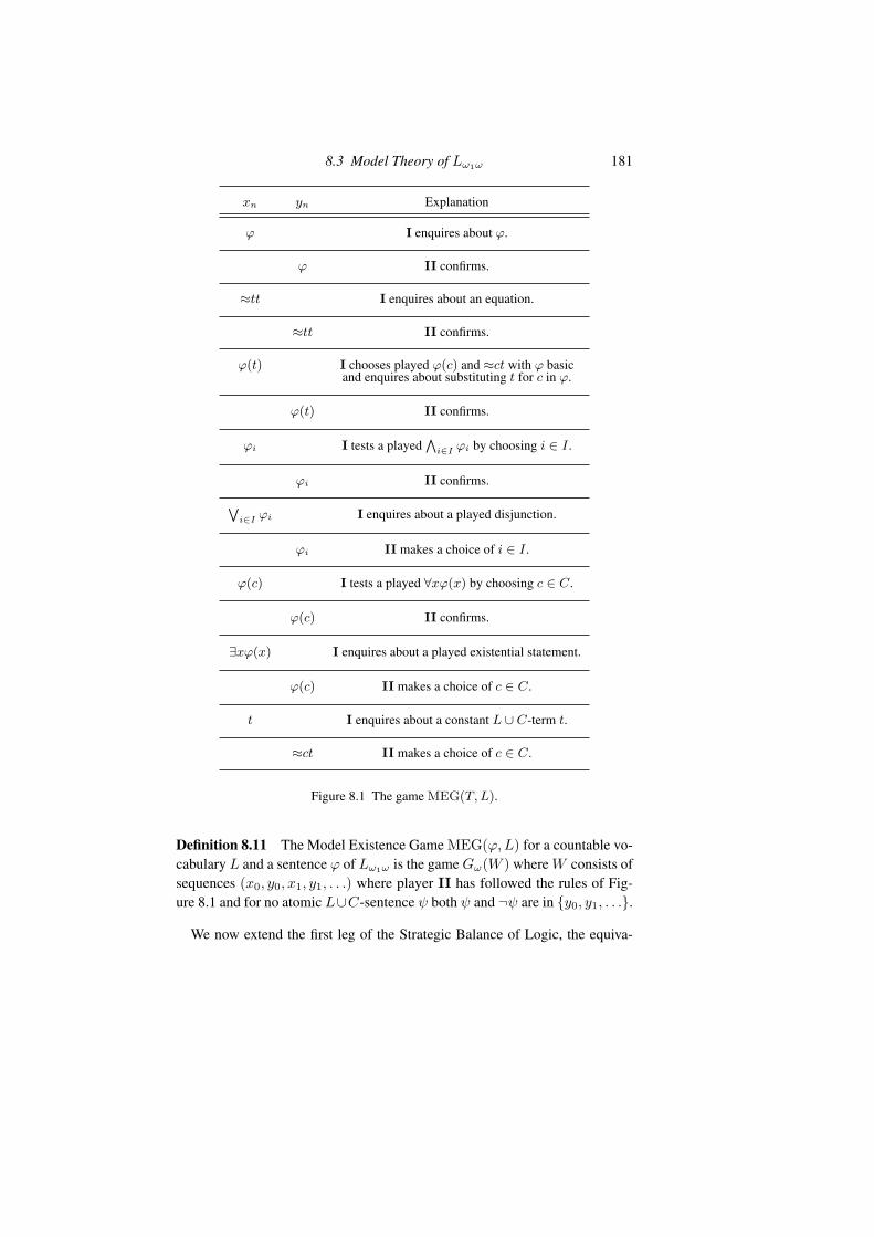
8.3 Model Theory of Lω1ω 181
xn yn Explanation
ϕ I enquires about ϕ.
ϕ II confirms.
≈tt I enquires about an equation.
≈tt II confirms.
ϕ(t) I chooses played ϕ(c) and ≈ct with ϕ basicand enquires about substituting t for c in ϕ.
ϕ(t) II confirms.
ϕi I tests a playedV
i∈I ϕi by choosing i ∈ I .
ϕi II confirms.
Wi∈I ϕi I enquires about a played disjunction.
ϕi II makes a choice of i ∈ I .
ϕ(c) I tests a played ∀xϕ(x) by choosing c ∈ C.
ϕ(c) II confirms.
∃xϕ(x) I enquires about a played existential statement.
ϕ(c) II makes a choice of c ∈ C.
t I enquires about a constant L ∪ C-term t.
≈ct II makes a choice of c ∈ C.
Figure 8.1 The game MEG(T, L).
Definition 8.11 The Model Existence Game MEG(ϕ, L) for a countable vo-cabulary L and a sentence ϕ of Lω1ω is the game Gω(W ) where W consists ofsequences (x0, y0, x1, y1, . . .) where player II has followed the rules of Fig-ure 8.1 and for no atomic L∪C-sentence ψ both ψ and ¬ψ are in {y0, y1, . . .}.
We now extend the first leg of the Strategic Balance of Logic, the equiva-

182 Model Theory of Infinitary Logic
lence between the Semantic Game and the Model Existence Game, from firstorder logic to infinitary logic:
Theorem 8.12 (Model Existence Theorem for Lω1ω) Suppose L is a count-able vocabulary and ϕ is an L-sentence of Lω1ω. the following are equivalent:
(1) There is an L-structure M such that M |= ϕ.(2) Player II has a winning strategy in MEG(ϕ, L).
Proof The implication (1) → (2) is clear as II can keep playing sentencesthat are true in M. For the other implication we proceed as in the proof ofTheorem 6.35. Let C = {cn : n ∈ N} and Trm = {tn : n ∈ N}. Let(x0, y0, x1, y1, . . .) be a play in which player II has used her winning strategyand player I has maintained the following conditions:
1. If n = 0, then xn = ϕ.2. If n = 2 · 3i, then xn is ≈cici.3. If n = 4 · 3i · 5j · 7k · 11l, yi is ≈cjtk, and yl is ϕ(cj), then xn is ϕ(ci).4. If n = 8 · 3i · 5j and yi is
�m∈N ϕm, then xn is ϕj .
5. If n = 16 · 3i and yi is�
m∈N ϕm, then xn is�
m∈N ϕm.6. If n = 32 · 3i · 5j , yi is ∀xϕ(x), then xn is ϕ(cj).7. etc.
The rest of the proof is exactly as in the proof of 6.35.
Our success in the above proof is based on the fact that even if we dealwith infinitary formulas we can still manage to let player I list all possibleformulas that are relevant for the consistency of the starting formula. If evenone uncountable conjunction popped up, we would be in trouble.
It suffices to consider in MEG(ϕ, L) such constant terms t that are eitherconstants or contain no other constants than those of C. Moreover, we mayassume that if player I enquires about ≈tt, then t = cn for some n ∈ N.
Corollary Let L be a countable vocabulary. Suppose ϕ and ψ are sentencesof Lω1ω. the following are equivalent:
(1) ϕ |= ψ(2) Player I has a winning strategy in MEG(ϕ ∧ ¬ψ, L).
The proof of Compactness Theorem does not go through, and should not,because there are obvious counter-examples to compactness in Lω1ω. In manyproofs where one would like to use the Compactness Theorem one can insteaduse the Model Existence Theorem. The non-definability of well-order in L∞ω
was proved already in Theorem 7.26 but we will now prove a stronger versionfor Lω1ω:
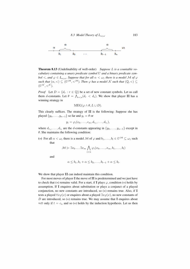
8.3 Model Theory of Lω1ω 183
Theorem 8.13 (Undefinability of well-order) Suppose L is a countable vo-cabulary containing a unary predicate symbol U and a binary predicate sym-bol <, and ϕ ∈ Lω1ω. Suppose that for all α < ω1 there is a model M of ϕsuch that (α, <) ⊆ (UM, <M). Then ϕ has a model N such that (Q, <) ⊆(UN , <N ).
Proof Let D = {dr : r ∈ Q} be a set of new constant symbols. Let us callthem d-constants. Let θ =
�r<s
(dr < ds). We show that player II has awinning strategy in
MEG(ϕ ∧ θ, L ∪D).
This clearly suffices. The strategy of II is the following: Suppose she hasplayed {y0, . . . , yn−1} so far and yi = θ or
yi = ϕi(c0, . . . , cm, dr1 , . . . , drl),
where dr1 , . . . , drl are the d-constants appearing in {y0, . . . , yn−1} except inθ. She maintains the following condition:
(�) For all α < ω1 there is a model M of ϕ and b1, . . . , bl ∈ UM ⊆ ω1 suchthat
M |= ∃x0 . . .∃xm
�
i<n
ϕi(x0, . . . , xm, b1, . . . , bl)
and
α ≤ b1, b1 + α ≤ b2, . . . , bl−1 + α ≤ bl.
We show that player II can indeed maintain this condition.For most moves of player I the move of II is predetermined and we just have
to check that (�) remains valid. For a start, if I plays ϕ, condition (�) holds byassumption. If I enquires about substitution or plays a conjunct of a playedconjunction, no new constants are introduced, so (�) remains true. Also, if Itests a played ∀xϕ(x) or enquires about a played ∃xϕ(x), no new constants ofD are introduced, so (�) remains true. We may assume that I enquires about≈tt only if t = cn and so (�) holds by the induction hypothesis. Let us then

184 Model Theory of Infinitary Logic
Figure 8.2
assume (�) holds and I enquires about a played disjunction�
i∈Iψi. For each
α < ω1 we have a model Mα as in (�) and some iα ∈ I such that Mα |= ψiα .Since I is countable, there is a fixed i ∈ I such that for uncountably manyα < ω1: Mα |= ψi. If II plays this ψi, condition (�) is still true.
The remaining case is that I enquires about a constant term t. We may as-sume t = dr as otherwise there is nothing to prove. The constants of D oc-curring so far in the game are dr1 , . . . , drl . Let us assume ri < r < ri+1. Toprove (�), assume α < ω1 and let β = α · 2. By the induction hypothesis thereis M as in (�) such that bi + β ≤ bi+1. Let dr be interpreted in M as bi + α.Now M satisfies the condition (�) (see Figure 8.3).
The following Corollary is due to Lopez-Escobar [LE66b].
Corollary If ϕ is a sentence of Lω1ω in a vocabulary which contains theunary predicate U and the binary predicate <, and (UM, <M) is well-orderedin every model of ϕ, then there is α < ω1 such that the order type of (UM, <M
) is < α for every model M of ϕ.
Corollary The class of well-orderings is not a PC-class of Lω1ω.
The undefinability of well-ordering as a PC-class of L∞ω will be estab-lished later. We now prove the Craig Interpolation Theorem for Lω1ω. Thereare several different proofs of this theorem, some of which employ the aboveCorollary directly. Our proof is like the original proof by Lopez-Escobar, ex-cept that we operate with model existence games instead of Gentzen systems.
Theorem 8.14 (Separation Theorem) Suppose L1 and L2 are vocabularies.Suppose ϕ is an L1-sentence of Lω1ω and ψ is an L2-sentence of Lω1ω such

Pages deleted for copyright reasons
1

202 Model Theory of Infinitary Logic
I II Winning condition
a0 ∈ Ab0 ∈ A ϕ0(a0, b0)
a1 ∈ Ab1 ∈ A ϕ1(a0, b0, a1, b1)
......
Figure 8.7 The game quantifier.
8.6 Game Logic
In this section we sketch the basic properties and applications of the so-calledclosed game quantifier of length ω
∀x0∃y0∀x1∃y1 . . .�
n<ω
ϕn(x0, y0 . . . , xn, yn) (8.18)
and its generalization, the so-called closed Vaught-formula of length ω
∀x0
�
i0∈I0
�
j0∈J0
∃y0∀x1
�
i1∈I1
�
j1∈J1
∃y1 . . .�
n<ω
ϕi0j0...injn(x0, y0 . . . , xn, yn)
(8.19)as well as their open counterparts. We use the general term game quantificationto cover expressions of the above type. The semantics of these expressions isdefined below by reference to a proper version of a Semantic Game.
The first application of game quantifiers in model theory was Svenonius’sTheorem [Sve65] to the effect that every PC-definable class of models isrecursively axiomatizable in countable models. Moschovakis [Mos72] intro-duced the game quantifier to descriptive set theory showing that inductive re-lations on countable acceptable structures are definable by the game quantifier.Vaught [Vau73] applied game expressions to develop a general definability the-ory for Lω1ω including a Covering Theorem. Subsequently game quantifiershave become a standard tool in model theory.
Closed game formulasWe shall first discuss the simpler case (8.18) and show how it can be used astechnical tool for an analysis of PC-definability in first order logic.
Definition 8.36 (Game quantifier) The truth of a game expression (8.18) ina model A means the existence of a winning strategy of player II in the gameof length ω of Figure 8.7. Player II wins this game if
8.6 Game Logic 203
A |= ϕn(a0, b0, . . . , an, bn)
for all n ∈ N. A winning strategy of II is a sequence {τn : n < ω} of functionson A such that
A |= ϕn(a0, τ0(a0), a1, τ1(a0, a1), . . . , an, τn(a0, . . . , an))
for all a0, a1, . . . in A.
Example 8.37 Examples of formulas of the form (8.18) are
1. ∃x0∃x1∃x2 . . .�
nxn+1 < xn, which in a linearly ordered model (A, <)
says that the linear order is not a well-order.2. ∃y∃z∀x0∀x1∀x2 . . .
�n((yEx0 ∧ x0Ex1 ∧ . . . xn−1Exn) → ¬≈xnz),
which in a graph says that the graph is not connected.3. ∀x0∀x1∀x2 . . .
�n>2((x0Ex1 ∧ . . .∧xn−1Exn ∧
�0≤i<j<n
¬≈xixj) →¬≈x0xn), which in a graph says that the graph is cycle-free.
As the above examples show, game expressions are more powerful thanL∞ω. In fact, we shall see below that they can express even things that gobeyond L∞∞. Therefore we cannot expect the model theory of game expres-sions to be as nice as that of Lω1ω. However, the game expressions permit onevery useful technique. This is the method of approximations, originally duein model theory to Keisler and then extensively used by Makkai, Vaught andothers.
We use xi, yi or just x, y, when the length of the sequences is clear from thecontext, to denote x0, y0, . . . , xi−1, yi−1.
Definition 8.38 Suppose Φ is the closed game formula (8.18). We shall asso-ciate Φ with a sequence Φn
γ,γ ∈ On, of L∞ω-formulas, called approximations,
as follows:
Φn
0 (xn, yn) =�
j<nϕj−1(xj , yj)
Φn
γ+1(xn, yn) = ∀xn∃ynΦn+1γ
(xn+1, yn+1)Φn
ν(x, y) =
�γ<ν
Φn
γ(x, y) for limit ν.
The trivial properties of these approximations are proved easily by transfi-nite induction:
• Φn
γ(x, y) ∈ Lκω for γ < κ
• qr(Φn
ν(x, y)) = ν for limit ν > 0
• |= Φ → Φ0γ
for all γ• |= Φn
γ(x, y) → Φn
β(x, y) for β ≤ γ.
Less trivial is the following important and characteristic property of the ap-proximations:
204 Model Theory of Infinitary Logic
Proposition 8.39 If |A| = κ and A |= Φ0α
for all α < κ+, then A |= Φ.
Proof We define a winning strategy {τn : n ∈ N} of II in the game (8.7) asfollows: Suppose a0, b0, ..., an−1, bn−1 have been played. The strategy of II isto maintain the property
For all α < κ+: A |= Φn
α(a0, b0, ..., an−1, bn−1). (8.20)
In the beginning this condition holds by assumption. Suppose the conditionholds after a0, b0, ..., an−1, bn−1 have been played. Now I plays an. If there isno bn such that
for all α < κ+ : A |= Φn+1α
(a0, b0, ..., an, bn), (8.21)
then for every bn ∈ A there is α(bn) < κ+ such that
A �|= Φn+1α(bn)(a0, b0, ..., an, bn).
Let δ = supbn∈A
α(bn). Note that δ < κ+. Hence by assumption A |=Φn
δ+1(a0, b0, ..., an−1, bn−1). We obtain immediately a contradiction. Thus theremust be a bn such that (8.21).
Corollary In countable models the game formula Φ and the Lω2ω-sentence�α<ω1
Φ0α
are logically equivalent.
Thus as far as countable models are concerned, the only thing that the closedgame formulas (8.18) add to Lω1ω is an uncountable conjunction. When wemove to bigger models, longer and longer conjunctions are needed, but that isall.
Definition 8.40 A structure in a countable recursive vocabulary is recursivelysaturated if it satisfies
∀x1...xn((�
n<ω
∃y�
m<n
ϕm(x1, ..., xn, y)) → ∃y�
n<ω
ϕn(x1, ..., xn, y))
for all recursive sequences {ϕm(x1, ..., xn, y) : m < ω} of first order formu-las.
Examples of recursively saturated structures are the dense linear order (Q, <), and the field (C,+, ·) of complex numbers. Every infinite model of a re-cursive vocabulary has a countable recursively saturated elementary extension(see [CK90, Section 2.4]).
Proposition 8.41 Suppose A is recursively saturated. Then A |= Φ ↔�n<ω
Φ0n
.
8.6 Game Logic 205
Proof We proceed as in the proof of Proposition 8.39. SupposeA |=�
n<ωΦ0
n.
We define a winning strategy {τn : n ∈ N} of II in the game (8.7) as follows.Suppose a0, b0, ..., an−1, bn−1 have been played. The strategy of II is to main-tain the property
For all m < ω: A |= Φn
m(a0, b0, ..., an−1, bn−1). (8.22)
In the beginning this condition holds by assumption. Suppose the conditionholds after a0, b0, ..., an−1, bn−1 have been played. Now I plays an. We lookfor bn such that
A |=�
m<ω
Φn+1m
(a0, b0, ..., an, bn), (8.23)
i.e. we want to show
A |= ∃yn
�
m<ω
Φn+1m
(a0, b0, ..., an, yn). (8.24)
Since A is ω-saturated, it suffices to prove
A |=�
m<ω
∃yn
�
k<m
Φn+1k
(a0, b0, ..., an, yn). (8.25)
Suppose m < ω is given. By (8.22) we have
A |= ∀xn∃ynΦn+1k
(a0, b0, ..., xn, yn).
By choosing the value of xn to be an we get b such that
A |= Φn+1k
(a0, b0, ..., an, b).
We have proved (8.25).
What about structures that are not recursively saturated? To conclude A |=Φ we have to assume A |= Φ0
αfor some infinite ordinals α, too. We refer to
Barwise [Bar75] for details.Barwise [Bar76] observed that game formulas can be used to “straighten”
partially ordered quantifiers. Consider the so called Henkin quantifier�∀x ∃y∀u ∃v
�ϕ(x, y, u, v, z) (8.26)
the meaning of which is
There are f and g such that for all a and b ϕ(a, f(a), b, g(b), z). (8.27)
We call formulas of the form (8.26), with ϕ(x, y, u, v) first order, Henkin-formulas. Indeed, they were introduced by Henkin [Hen61]. An alternative

206 Model Theory of Infinitary Logic
notation for Henkin-formulas is offered by dependence logic [Vaa07]:
∀x∃y∀u∃v(=(u, z, v) ∧ ϕ(x, y, u, v, z)),
where the intuitive interpretation of =(u, z, v) is “v depends only on u and z”.Let us compare (8.26) with the game formula
∀x0∃y0∀u0∃v0∀x1∃y1∀u1∃v1 . . .�i,j,k,l
((≈xixj ∧ ≈ukul) → (≈yiyj ∧ ≈vkvl ∧ ϕ(xi, yi, ui, vi, z))).(8.28)
Clearly, (8.26), or rather (8.27), implies (8.28) as II can let yn = f(xn)and vn = g(un). In a countable model the converse is true: Suppose A is acountable model and s is an assignment. Let (an, bn), n ∈ N, list all pairs ofelements of A. Let us play the game associated with the formula (8.28) in Aso that I plays xn = an and un = bn. Let the responses of II be yn = a∗
n
and vn = b∗n
. Let f(an) = a∗n
and g(bn) = b∗n
. It is easy to see that A |=s
ϕ(an, f(an), bm, g(bm), z) for all n and m. Thus (8.26) holds in A under theassignment s. We have proved:
Proposition 8.42 The formulas (8.26) and (8.28) are equivalent in all count-able models.
In consequence, in a countable recursively saturated model (8.26) is, byProposition 8.41, equivalent to
�n<ω
Φ0n
.Let us say that {ϕn : n < ω} is a first order axiomatization of a class K of
models, if the following are equivalent for all first order ψ:
1. ψ is true in all models in K.2. {ϕn : n < ω} |= ψ.
Proposition 8.43 {Φ0n
: n < ω} is a first order axiomatization of the classof models of (8.26).
Proof Suppose a first order sentence ψ follows from (8.26). We show that itfollows from {Φ0
n: n < ω}. If not, then there is a model A of {Φ0
n: n < ω}
which satisfies ¬ψ. Take a countable recursively saturated model of the firstorder theory {Φ0
n: n < ω} ∪ {¬ψ}. We get a contradiction.
Example 8.44 (Models with an involution) Suppose L is the vocabulary {R},where R is (for simplicity) binary. The class of L-models with an involution(non-trivial automorphism of order two) can be axiomatized by the Henkin-sentence
Φ = ∃z�∀x ∃y∀u ∃v
�ϕ(x, y, u, v, z),
8.6 Game Logic 207
where ϕ(x, y, u, v, z) is the conjunction of (≈xu → ≈yv), (≈xv → ≈yu),(Rxu ↔ Ryv), and≈xz → ¬≈xy. In countable models this Henkin-sentenceis equivalent to
∃z∀x0∃y0∀u0∃v0∀x1∃y1∀u1∃v1 . . .�i,j,k,l
((≈xixj ∧ ≈ukul) → (≈yiyj ∧ ≈vlvk ∧ ϕ(xi, yi, ui, vi, z))).
By inspecting the approximations Φ0n
of Φ we see that a first order sentencehas a model with an involution if and only if it is consistent with the set of thefirst order sentences
∃z∀x0∃y0∀x1∃y1 . . .∀xm∃ym�i,j,k,l≤m
((≈xixj → ≈yiyj) ∧ (≈xiyj → ≈xjyi)∧(≈xiz → ¬≈xiyi) ∧ (Rxixj ↔ Ryiyj)),
where m ∈ N.
The above result about Henkin-formulas are not limited to the particularform of (8.26). The meaning of the more general formula
0
B@
∀xi11. . . ∀xi1m1
∃y1
......
...∀xin
1. . . ∀xin
mn∃yn
1
CA ϕ(xi11, . . . , xi1m1
, y1, . . . , xin1, . . . , xin
mn, yn, z) (8.29)
is simply: There are f1, ..., fn such that for all ai11, . . . , ai1m1
(i = 1, ..., n),
ϕ(ai11, . . . , ai1m1
, b1, . . . , ain1, . . . , ain
mn, bn, z),
where
bj = fj(aij1, . . . , a
ijmj
), for j = 1, ..., n.
Note that (8.29) makes perfect sense even if the rows of the quantifier prefixare of different lengths, as in
�∀x1∀x2 ∃y∀u ∃v
�ϕ(x1, x2, y, u, v, z). (8.30)
We call all formulas of the form (8.29) Henkin-formulas. Let Φ be obtainedfrom (8.29) as (8.28) was obtained from (8.26). The following proposition isproved mutatis mutandis as in Proposition 8.42:
Proposition 8.45 The formulas (8.29) and Φ are equivalent in all countablemodels.

208 Model Theory of Infinitary Logic
In consequence, in a countable recursively saturated model (8.29) is, byProposition 8.41, equivalent to
�n<ω
Φ0n
.Enderton [End70] and Walkoe [Wal70] observed that any PC-class can be
defined by a Henkin-formula:
Theorem 8.46 For every PC-class K there is a Henkin-sentence Φ such thatfor all M:
M ∈ K ⇐⇒ M |= Φ.
Proof Suppose K is the class of reducts of a first order sentence ϕ. We mayassume that ϕ is of the form
∀x1 . . .∀xmψ, (8.31)
where ψ is quantifier free but contains new function symbols f1, ..., fn. (Thisis the so called Skolem Normal Form of ϕ). We will perform some reductionson (8.31) in order to make it more suitable for the construction of ϕ.
Step 1: If ψ contains nesting of the function symbols f1, . . . , fn or of the func-tion symbols of the vocabulary, we can remove them one by one by using theequivalence of
|= θ(fi(t1, . . . , tm))
and
∀x1 . . .∀xm((t1 = x1 ∧ . . . ∧ tm = xm) → θ(fi(x1, . . . , xm)))
for any first order θ. Thus we may assume that all terms occurring in ψ are ofthe form xi or fi(xi1 , . . . , xik).
Step 2: If ψ contains an occurrence of a function symbol fi(xi1 , . . . , xik) withthe same variable occurring twice, e.g. is = ir, 1 < r < k, we can removesuch by means of a new variable xl and the equivalence
|= ∀x1 . . .∀xmθ(fi(xi1 , . . . , xik)) ↔∀x1 . . .∀xm∀xl(xl = xr → θ(fi(xi1 , . . . , xir−1 , xl, xir+1 , . . . , xik)))
for any first order θ. Thus we may assume that if a term such as fi(xi1 , . . . , xik)occurs in ψ, its variables are all distinct.
Step 3: If ψ contains two occurrences of the same function symbol but withdifferent variables or with the same variables in different order, we can removesuch by using appropriate equivalences. If {i1, ..., ik} ∩ {j1, ..., jk} = ∅, wehave the equivalence
|= ∀x1 . . .∀xmθ(fi(xi1 , . . . , xik), fi(xj1 , . . . , xjk)) ↔
8.6 Game Logic 209
∃f �i∀x1 . . .∀xm(θ(fi(xi1 , . . . , xik), f �
i(xj1 , . . . , xjk)) ∧
((xi1 = xj1 ∧ . . . ∧ xik = xjk) →fi(xi1 , . . . , xik) = f �
i(xj1 , . . . , xjk)))
for any first order θ. We can reduce the more general case, where {i1, ..., ik}∩{j1, ..., jk} �= ∅, to this case by introducing new variables, as in Step 2. Thuswe may assume that for each function symbol fi occurring in ψ there areji
1, . . . , ji
nisuch that all occurrences of fi are of the form fi(xj
i1, . . . , xji
mi)
and ji
1, . . . , ji
miare all different from each other.
In sum we may assume the function terms that occur in ψ are of the formfi(xj
i1, . . . , xji
mi) and for each i the variables xj
i1, . . . , xji
miand their order is
the same. Let N be greater than all the xjik. Let Φ be the Henkin-sentence
∀xj11
. . . ∀xj1m1
∃xN+1
......
...∀xj
n1
. . . ∀xjnmn
∃xN+n
ψ�
where ψ� is obtained from ψ by replacing fi(xji1, . . . , xji
mi) everywhere by
xN+i. This is clearly the desired Henkin-sentence. In the notation of depen-dence logic ([Vaa07]) this would look like:
∀x1 . . .∀xm∃xN+1 . . .∃xN+n (=(xj11, . . . , xj1
m1, xN+1) ∧
. . .
=(xjn1, . . . , xjn
mn, xN+n) ∧ ψ�).
By combining the above observations we get the following result of Sveno-nius [Sve65]:
Theorem 8.47 For every PC-class K there is a closed game sentence Φ anda sequence ϕn of first order sentences such that for all structures M:
1. If M ∈ K, then M |= Φ and M |= ϕn for all n ∈ N.2. If M |= Φ and M is countable, then M ∈ K.3. If M |=
�n
ϕn and M is countable recursively saturated, then M ∈ K.4. If ψ is any first order sentence, then ψ has a model in K if and only if ψ is
consistent with {ϕn : n < ω}.
Moreover, the sequence {ϕn : n ∈ N} (or rather the set of Godel-numbers ofthe ϕn) is recursive.

Pages deleted for copyright reasons
1
9Stronger Infinitary Logics
9.1 Introduction
The infinitary logics Lκω, L∞ω and L∞G of the previous chapter had one im-portant feature in common with first order logic: the truth predicate of theselogics is absolute1 in set theory. We now move on to logics which do not havethis property. We lose something but we also gain something else. For example,we lose the last remnants of the Completeness Theorem of first order logic. Onthe other hand, we can express deeper properties of models, such as uncount-ability, completeness of a separable order, and other properties, too. Perhapssurprisingly, some methods, such as the method of Ehrenfeucht-Fraısse games,still work perfectly even with these strong logics.
9.2 Infinite Quantifier Logic
First order logic and the infinitary logic L∞ω are able to express
∃V ϕ and ∀V ϕ
when V is any finite set of variables. In the infinite quantifier logics of thissection we can express this even when V is an infinite set of variables.
Before actually defining the infinite quantifier logics, we first define the ap-propriate version of the Ehrenfeucht-Fraısse game. In this game the playersplay sequences of a given length. Each round consists of a choice of a sequenceby I followed by a choice of a sequence by II. The goal of II is to make surethe played sequences form, element by element, a partial isomorphism. Thus
1 More exactly, if M is a transitive model of ZFC containing A and ϕ as elements, then A is amodel of ϕ if and only if the set-theoretical statement “A |= ϕ” holds in the model M .

9.2 Infinite Quantifier Logic 229
if I plays a sequence
x0 = (x0(0), . . . , x0(n), . . .)
which is a descending sequence relative to a linear order < in one of the mod-els, player II tries to play likewise a sequence
y0 = (y0(0), . . . , y0(n), . . .)
which constitutes a descending sequence relative to < in the other model. Ifthat other model is well-ordered by <, she loses right away. Note that play-ers have made so far just one move each, albeit a move with infinitely manycomponents.
For another example, suppose one of the models is countable while the otheris uncountable. If player I is allowed to play countable sequences he can imme-diately let x0 enumerate the countable model. Whichever countable sequenceII plays, I wins during the next round by playing an element from the uncount-able model which is different from all the elements played by II.
To define the new game more exactly, we fix some notation. A functions : α → M is called a sequence of length len(s) = α. The set of all sequencesof length α of elements of M is denoted by Mα. We define
M<α =�
β<α
Mβ
and
Partκ(A,B) = {p ∈ Part(A,B) : |p| < κ}.
Now we can define the new Ehrenfeucht-Fraısse Game:
Definition 9.1 Suppose κ is a cardinal. The Ehrenfeucht-Fraısse game withmoves of size < κ onM andM�, denoted EFκ
ω(M,M�), is the game in which
player I plays
xn ∈ M<κ ∪ (M �)<κ
and II responds with
yn ∈ M<κ ∪ (M �)<κ
for all n ∈ N. Player II wins if for all n,
(1) len(xn) = len(yn)(2) xn ∈ M<κ ↔ yn ∈ (M �)<κ

Pages deleted for copyright reasons
1
9.3 The Transfinite Ehrenfeucht-Fraısse Game 249
9.3 The Transfinite Ehrenfeucht-Fraısse Game
All our games up to now have had at most ω rounds. There is no difficultyin imagining what a game of, say, length ω + ω would look like: it would belike playing two games of length ω one after the other. For example, it is bynow well known to the reader that the second player has a winning strategy inthe Ehrenfeucht-Fraısse game of length ω on (R, <) and (R \ {0}, <). But ifplayer I is allowed one more move after the ω moves, he wins.
For a more enlightening example, suppose M and N are equivalence re-lations such that M has ℵ1 countable classes and ℵ0 uncountable classeswhile N has ℵ1 countable classes and ℵ1 uncountable classes. Does II have awinning strategy in EFω. Yes! She just keeps matching different equivalenceclasses with different equivalence classes. But she can actually win the gameof length ω + ω, too! During the first ω moves she matches countable equiv-alence classes with countable ones and uncountable equivalence classes withuncountable ones. After the first ω moves she may have to match a countableequivalence class with an uncountable class, but I will not be able to call II’sbluff. It is only when I has ω + ω + 1 moves that he has a winning strategy:During the first ω moves I plays one element from each uncountable class ofM. Then I plays one element b from an unused uncountable equivalence classof N . Player II will match this element with an element c from a countableequivalence class of M. During the next ω rounds player I enumerates thecountable equivalence class of c. Finally he plays an unplayed element equiv-alence to b. Player II loses as all elements equivalent to c have been playedalready.
Let L be a vocabulary and A0 and A1 two L-structures. We give a rigorousdefinition of a transfinite version of the Ehrenfeucht-Fraısse Game on the twomodels A0 and A1. We let the number of rounds of this game be an arbitraryordinal δ.
In the sequel we allow the domains of M0 and M1 to intersect and incor-porate a mechanism to account for this..
We shall all the time refer to sequences
z = �zα : α < δ�, where zα = (cα, xα),
of elements of {0, 1} × (A0 ∪ A1). If y = �yα : α < δ� is a sequence ofelements of A0 ∪A1, the relation
pz,y ⊆ (A0 ∪A1)2
is defined as follows:
pz,y = {(aα, bα) : α < δ}

250 Stronger Infinitary Logics
I z0 z1 . . . zα . . . (α < δ)
II y0 y1 . . . yα . . . (α < δ)
Figure 9.6 The Ehrenfeucht-Fraısse Game
where
aα =�
xα if cα = 0yα if cα = 1
bα =�
yα if cα = 0xα if cα = 1.
Remark We shall often use the fact that pz,y = ∪σ<δpz�σ,y�σif δ is a limit
ordinal.
We are interested in the question whether
pz,y ∈ Part(A0,A1) (9.5)
or not. In the Ehrenfeucht-Fraısse Game one player chooses z trying to make(9.5) false, and the other player chooses y trying to make (9.5) true. Let
Seqδ(A0, A1)
be the set of all sequences �(cα, xα) : α < δ� where cα ∈ {0, 1} and xα ∈Acα .
Definition 9.46 Let δ ∈ On. The Ehrenfeucht-Fraısse game of length δ onA0 and A1, in symbols
EFδ(A0,A1)
is defined as follows. There are two players I and II . During one round of thegame player I chooses an element cα of {0, 1} and an element xα of Acα , andthen player II chooses an element yα of A1−cα . Let zα = (cα, xα). There areδ rounds and in the end we have z = �zα : α < δ� and y = �yα : α < δ�.We say that player II wins this sequence of rounds, if pz,y ∈ Part(A0,B1).Otherwise player I wins this sequence of rounds.
The above definition is useful as an intuitive model of the game. However,it is not mathematically precise because we have not defined what choosing anelement means. The idea is that a player is free to choose any element. Also,we are really interested in the existence of a winning strategy for a player bymeans of which he can win every sequence of rounds. The following exactdefinition of a winning strategy is our mathematical model for the intuitiveconcept of a game.

9.3 The Transfinite Ehrenfeucht-Fraısse Game 251
Definition 9.47 A strategy of II in EFδ(A0,A1) is a sequence
τ = �τα : α < δ�
of functions such that
dom(τα) = Seqα+1(A0, A1)
and
rng(τα) ⊆ A0 ∪A1
for each α < δ. If z ∈ Seqδ(A0, A1) and y = �yα : α < δ�, where
yα = τα(z�α+1)
for all α < δ, then we denote pz,y by pz,τ . The strategy τ of II is a winningstrategy if pz,τ ∈ Part(A0,A1) for all z ∈ Seq
δ(A0, A1). A strategy of I in
EFδ(A0,A1) is a sequence
ρ = �ρα : α < δ�
of functions such that
rng(ρα) ⊆ {0, 1}× (A0 ∪A1)
and dom(ρα) is defined inductively as follows: dom(ρα) is the set of se-quences y = �yβ : β < α� such that for all β < α,
yβ ∈�
A1, if ρβ(y�β) = (0, x) for some x
A0, if ρβ(y�β) = (1, x) for some x.
If y = �yα : α < δ� ∈ dom(ρ) (i.e �yα : α < β� ∈ dom(ρβ) for all β < δ)and z = �zα : α < δ� satisfy
ρα(y�α) = zα,
then pz,y is denoted by pρ,y . The strategy ρ is a winning strategy of I if thereis no y ∈ dom(ρ) such that pρ,y ∈ Part(A,B). We say that a player winsEFδ(A0,A1) if he has a winning strategy in it.
Remark If τ = �τα : α < δ� is a strategy of II in EFδ(A0,A1) and σ < δ,then τ�
σ= �τα : α < σ� is a strategy of II in EFσ(A0,A1). If τ is winning,
then so is τ�σ
. Moreover, if z ∈ Seqδ(A0 ∪ A1), then pz�σ,τ�σ
⊆ pz,τ . If δ isa limit ordinal, we have pz,τ = ∪σ<δpz�σ,τ�σ
and τ is winning if and only ifτ�
σis winning for all σ < δ.
252 Stronger Infinitary Logics
Example 9.48 Let L = ∅. Let A0 and A1 be two L-structures of cardi-nalities κ and λ respectively. Let us first assume δ ≤ κ ≤ λ. Then II winsEFδ(A0,A1). Her winning strategy τ = �τα : α < δ� is defined as follows.Let F (X) ∈ X for every non-empty X ⊆ A0 ∪ A1. Suppose τα is definedfor α < σ, where σ < δ. We define τσ . For any z = �(cα, xα) : α < σ�, letYz = {xζ : ζ < σ} ∪ {τζ(z�
ζ+1) : ζ + 1 < σ}. Let now
τσ(z�σ+1) =
τζ(z�ζ+1) if xσ = xζ , ζ < σ
xζ if xσ = τζ(z�ζ+1), ζ < σ
F (A1−ci \ Yz�σ) otherwise.
It is clear that for all z the relation pz,τ is a partial isomorphism. In fact itsuffices that pz,τ is a one-one function, since L = ∅.
Let us then assume κ < λ and κ < δ. Then I wins EFδ(A0,B1). Hiswinning strategy ρ = �ρα : α < δ� is defined as follows. Let A0 = {uη : η <κ}.
ρα(�yη : η < α�) =�
uα if α < κF (A1 \ {ρζ(�yη : η < ζ�) : ζ < α}) if κ ≤ α < δ.
The intuitive argument behind Example 9.48 based on Definition 9.46 canbe described very succinctly: If δ ≤ κ ≤ λ, the strategy of II is to copy theold moves if I plays an old element and choose some new element if I playsa new element. The assumption δ ≤ κ < λ guarantees that there are enoughelements to choose from. If κ < δ, the strategy of I is to first enumerate A0
during the first κ rounds of the game and then pick an element xκ ∈ A1, whichhas not been played yet by II. Then II has no elements in A0 left to play andhe loses the game.
Lemma 9.49 (i) If II wins the game EFα(A0,A1) and β < α, then II winsthe game EFβ(A0,A1).
(ii) If I wins the game EFα(A0,A1) and α < β, then I wins the gameEFβ(A0,A1).
(iii) There is no α such that both II and I win EFα(A0,A1).
Proof (i) If �τξ : ξ < α� is a winning strategy of II in EFα(A0,A1), then�τξ : ξ < β� is a winning strategy of II in EFβ(A0,A1).
(ii) If �ρξ : ξ < α� is a winning strategy of I in EFα(A0,A1), then �ρξ :ξ < β� is a winning strategy of I in EFβ(A0,A1), where
ρξ(�yη : η < ξ�) = ρα(�yη : η < α�)
for α ≤ ξ < β.

9.3 The Transfinite Ehrenfeucht-Fraısse Game 253
(iii) Suppose �τξ : ξ < α� is a winning strategy of II and �ρξ : ξ < α� awinning strategy of I in EFα(A0,A1). Define inductively
xξ = ρξ(�yη : η < ξ�)yξ = τξ(�xη : η ≤ ξ�).
If z = �xξ : ξ < α� and y = �yξ : ξ < α�, then pz,y is a partial isomorphismbecause II wins, and not a partial isomorphism because I wins, a contradiction.
Lemma 9.50 (i) If A0∼= A1, then II wins EFα(A0,A1) for all α.
(ii) If A0 �∼= A1, then I wins EFα(A0,A1) for all α ≥ |A0|+ |A1|.
Proof (i) Suppose f : A0∼= A1. Let
τξ(�(cη, xη) : η ≤ ξ�) =�
f(xξ) if cξ = 0f−1(xξ) if cξ = 1.
Then �τξ : ξ < α� is a winning strategy of II in EFα(A0,A1).(ii) Let {0, 1}× (A0 ∪A1) = {zξ : ξ < α} and ρ = �ρξ : ξ < α�, where
ρξ(�yη : η < ξ�) = zξ
for ξ < α. For any y = �yξ : ξ < α� the relation pρ,y is a partial isomorphismbetween A0 and A1. Since no isomorphism exists, ρ is a winning strategy ofI.
Corollary (i) If I wins EFα(A0,A1), then A0 �∼= A1.(ii) If II wins EFα(A0,A1), where α ≥ |A0|+ |A1|, then A0
∼= A1.
There is always at least one α for which II wins EFα(A0,A1), namelyα = 0. If A0
∼= A1, then by Lemma 9.49 and 9.50 there cannot be any α forwhich I wins EFα(A0,A1). But if A0 �∼= A1, then I wins EFα(A0,A1) fromsome α onwards.
There may be ordinals α for which neither player has a winning strategy(Exercises 9.29 and 9.30 below). Then the game is non-determined. The gameof length ω1 may also be non-determined, see [MSV93]. There may also bea limit ordinal α such that II wins EFβ(A0,A1) for each β < α but notEFα(A0,A1). We already know that this can happen if α = ω.
Lemma 9.51 Let L be a vocabulary and α an ordinal. The relation
A0 ∼α A1 ⇔ ∃ wins EFα(A0,A1)
is an equivalence relation on Str(L).

254 Stronger Infinitary Logics
Proof Reflexivity of ∼α follows from Lemma 9.50(i). In fact, II wins thegame EFα(A0,A0) with the trivial strategy τξ(�(cη, xη) : η ≤ ξ�) = xξ. Sym-metry is also trivial: Suppose II wins EFα(A0,A1) with τ = �τξ : ξ < α�.The following strategy τ � = �τ �
ξ: ξ < α� is winning for II in EFα(A1,A0):
τ �((cη, xη) : η ≤ ξ) = τ((1− cη, xη) : η ≤ ξ).
To see this, suppose z = �zξ : ξ < α� is given. Then pz,τ is a partial isomor-phism between A0 and A1, and the relation
p�z,τ
= {(b, a) : (a, b) ∈ pz,τ}
is a partial isomorphism between A1 and A0, witnessing the victory of II inEFα(A1,A0). To prove transitivity of ∼α, suppose τ = �τα : ξ < α� is awinning strategy of II in EFα(A0,A1) and τ � = �τ �
ξ: ξ < α� is a win-
ning strategy of II in EFα(A1,A2). We describe a winning strategy τ �� =�τ ��
ξ: ξ < α� of II in EFα(A0,A2). The idea is that II plays EFα(A0,A1)
and EFα(A1,A2) simultaneously. Suppose z�� = �(c��η, x��
η) : η ≤ ξ� ∈
Seqξ+1(A0, A1). We define by induction over η ≤ ξ the sequences z =
�(cη, xη) : η ≤ ξ�, z� = �(c�η, x�
η) : η ≤ ξ�, and τ �� = �τ ��
ξ: ξ < α� as
follows:
If c��η
= 0 1
Then (cη, xη) = (0, x��η) (1, τ �
η(z��
η))
(c�η, x�
η) = (0, τη(z�
η)) (1, x��
η)
τ ��η(z���
η) = τ �
η(z��
η) τη(z�
η)
Now �τ ��ξ
: ξ < α� is a winning strategy of II in EFα(A0,A2).
The relations ∼α form a sequence of finer and finer partitions of Str(L),starting from the one-class partition ∼0 and eventually approaching the ulti-mate refinement ∼= of every ∼α.
9.4 A Quasi-order of Partially Ordered Sets
Before we define the dynamic version of the transfinite game EFα we developsome useful theory of po-sets.
Definition 9.52 Suppose P and P � are po-sets. We define
P ≤ P �
if there is a mapping f : P → P � such that for all x, y ∈ P :
x <P y → f(x) <P� f(y).

9.4 A Quasi-order of Partially Ordered Sets 255
We write P < P �, if P ≤ P � and P � �≤ P , and we write P ≡ P �, if P ≤ P �and P � ≤ P.
Note that≤ is a transitive relation among po-sets. The≡-classes of≤ form aquasi-ordered class. This quasi-order is the topic of this section. It is not a totalorder, for there are incomparable po-sets, for example (ω, <) and its inverseordering (ω, >). For simplicity, we call ≤ itself the quasi-order of po-sets,without recourse to the ≡-classes.
Definition 9.53 Suppose P is a po-set. The tree σP is defined as follows. Itsdomain is the set of functions s with dom(s) ∈ On such that for all α,β ∈dom(s)
α < β → s(α) <P s(β).
The order is
s ≤ s� ↔ s = s��dom(s).
σ�P is the suborder of σP consisting of sequences s ∈ σP of successor length.
The σ-operation was introduced by Kurepa [Kur56] and studied further e.g.in [HV90] and [TV99].
Example 9.54 For any ordinal α let Bα be the tree of descending sequencesβ0 > . . . > βn of elements of α ordered by end-extension. Show that α ≤ β(as ordinals) if and only if Bα ≤ Bβ as po-sets. Every well-founded tree is≡-equivalent to some Bα. (See Exercise 9.36.)
Lemma 9.55 (i) σ�P ≤ P .(ii) σP �≤ P .(iii) σ�P < σP .(iv) If T is a tree, then T ≡ σ�T .
Proof (i) If s ∈ σ�P , let f(s) = s(dom(s) − 1). Then f : σ�P → P isorder-preserving.
(ii) Suppose f : σP → P were order-preserving. Define inductively s :On → P by s(α) = f(s�
α). Since α < β implies s(α) <P s(β), we get the
result that P is a proper class, a contradiction.(iii) σ�P ≤ σP trivially. On the other hand, if σP ≤ σ�P , then σP ≤ P
contrary to (ii),(iv) We know already σ�T ≤ T . Suppose t ∈ T and �tα : α ≤ β� is the
set of t� ∈ T with t� ≤T t in ascending order. Let dom(s) = β + 1 andst(α) = tα. then st ∈ σ�T and t �→ st is order-preserving.
256 Stronger Infinitary Logics
Example 9.56 Q �≤ σQ since σQ is well-founded while Q is not. In partic-ular Q �≤ σ�Q. Hence σ�Q < Q. Note that σ�Q is a special tree while σQ isnon-special. (See Exercise 9.40.)
Lemma 9.57 There is no sequence P0,P1, . . . so that σPn+1 ≤ Pn for alln < ω.
Proof Suppose fn : σPn+1 → Pn is order-preserving. For each fixed α, letsn
α∈ Pn so that
fn(�sn+1β
: β < α�) = sn
α.
Then each Pn is a proper class, a contradiction.
Definition 9.58 SupposeP andP � are po-sets. The game G(P,P �) is definedas follows. Player I plays p0 ∈ P , then player II plays p�0 ∈ P �. After thisI plays p1 ∈ P with p0 <P p1, and then player II plays p�1 ∈ P � withp�0 <P� p�1, and so on. At limits player I moves first pν ∈ P with pα <P pν forall α < ν. Then II moves p�
ν∈ P � with p�
α<P p�
νfor all α < ν. If a player
cannot move, he loses and the other player wins. Since P and P � are sets, oneof the players eventually wins.
Lemma 9.59 (i) σ�P ≤ P � if and only if II wins G(P,P �).(ii) If P is a tree, then P ≤ P � if and only if II wins G(P,P �).
Proof (i) Suppose f : σ�P → P � is order-preserving. If I has played p0 <. . . < pα in G(P,P �), II plays p�
α= f((p0, . . . , pα)). In this way she ends
up the winner. Conversely, suppose II wins G(P,P �) and s ∈ σ�P withdom(s) = α + 1. Let us play G(P,P �) so that I plays pβ = s(β) for β ≤ αand II uses her winning strategy. After I plays pα, II plays p�
α. If we define
f(s) = p�α
, we get an order-preserving mapping σ�P → P . This ends theproof of (i). (ii) follows from (i) and Lemma 9.55 (iv).
Lemma 9.60 σP � ≤ P if and only if I wins G(P,P �).
Proof Suppose f : σP � → P is order-preserving. If II has played
p�0 < . . . < p�β
< . . . (β < α) (9.6)
in G(P,P �), I plays pα = f((p�0, . . . , p�β , . . .)) in P �. In this way I winsG(P,P �). On the other hand, if I wins G(P,P �) and (9.6) is an ascend-ing chain in P �, we can let I play against the moves p�0, . . . , p
�β, . . . of II in
G(P,P �). Finally I plays pα according to his winning strategy. We let
f((p�0, . . . , p�β, . . .)) = pα.
Now f : σP � → P is order-preserving.

9.4 A Quasi-order of Partially Ordered Sets 257
Example 9.61 Suppose S ⊆ ω1. Let T (S) be the tree of closed ascend-ing sequences of elements of S. Choose disjoint stationary sets S1 and S2.Then T (S1) �≤ T (S2) and T (S2) �≤ T (S1) (Exercise 9.35). Thus the gameG(T (S1), T (S2)) is non-determined.
Definition 9.62 We use Tλ,κ to denote the class of trees of cardinality ≤ λwithout branches of length κ.
The simplest uncountable tree in Tκ,κ is the κ-fan which consists of branchesof all lengths < κ joined at the root, or in symbols,
Fκ = {sα : 0 < α < κ}, sα = �aα
β: β < α�,
aα
0 = 0, aα
β= (α,β) for β > 0,
ordered by end-extension. Aronszajn trees are in Tℵ1,ℵ1 . The trees T (S) ofExample 9.61 are in T2ω,ℵ1 .
Definition 9.63 A tree T is a persistent if for all t ∈ T and all α < ht(T )there is t� ∈ T such that t <T t� and ht(t�) ≥ α.
Persistency is a kind of non-triviality assumption for a tree. It means thatfrom any node you can go as high as you like. The κ-fan is certainly non-persistent. On the other hand, the tree
Tκ
p= (Fκ)<ω, (sα0 , ..., sαn−1) ≤ (sβ0 , ..., sβm−1) ⇐⇒
n ≤ m and αi = βi for i < n
is persistent and indeed the ≤-smallest persistent tree in Tκ,κ (Exercise 9.41).
Definition 9.64 A po-set P is a bottleneck in a class K of po-sets if P � ≤ Por P ≤ P � for all P � in the class K. A tree T is a strong bottleneck for a classK if the game G(T,P) is determined for all P ∈ K.
Every well-founded tree is a strong bottleneck in the class of all trees. IfS ⊆ ω1 is bistationary, then T (S) is by Example 9.61 not a bottleneck inthe class of all trees. The smallest persistent tree Tκ
pis a strong bottleneck in
the class Tκ,κ (Exercise 9.42). It is an interesting problem whether there arebottlenecks in the class Tκ,κ above Tκ
p. The following partial result is known:
Theorem 9.65 Suppose κ is a regular cardinal and and P is the forcingnotion for adding κ+ Cohen subsets to κ, then P forces that there are nobottlenecks in the class Tκ,κ above Tκ
p.
258 Stronger Infinitary Logics
Proof Suppose T is a bottleneck. Let α < κ+ such that T ∈ V [Gα]. LetAα be the Cohen subset of κ added at stage α. Note that Aα is a bistationarysubset of κ. We first show that � T �≤ T (Aα). Suppose
p � f : T (Aα) → T is strictly increasing.
When we force with Aα, calling the forcing notion P �, an uncountable branchappears in T (Aα), hence also in T . The product forcing Pα � P � contains aκ-closed dense set (Exercise 9.45). Hence it cannot add a branch of lengthκ to T . We have shown that T (Aα) �≤ T in V [G]. Since T is a bottleneck,T ≤ T (Aα). By repeating the same with −Aα we get T ≤ T (−Aα). Insum, T ≤ T (Aα) ⊗ T (−Aα) (see Exercise 9.44 for the definition of ⊗). ButT (Aα)⊗ T (−Aα) ≤ Tκ
p(Exercise 9.46). Hence T ≤ Tκ
p.
It is also known ([TV99]) that if V = L, then there are no bottlenecks in theclass Tℵ1,ℵ1 above Tℵ1
p.
9.5 The Transfinite Dynamic Ehrenfeucht-Fraısse Game
In this section we introduce a more general form of the Ehrenfeucht-FraısseGame. The new game generalizes both the usual Ehrenfeucht-Fraısse Gameand the dynamic version of it. In this game player I makes moves not only inthe models in question but also moves up a po-set, move by move. The gamegoes on as long as I can move. This game generalizes at the same time thegames EFα(A0,A1) and EFDδ(A0,A1). Therefore we denote it EFP ratherthan by EFDP .
If P is a po-set, let b(P) denote the least ordinal δ so that P does not havean ascending chain of length δ.
Definition 9.66 Suppose A0 and A1 are L-structures and P is a po-set. TheTransfinite Dynamic Ehrenfeucht-Fraısse Game EFP(A0,A1) is like the gameEFδ(A0,A1) except that on each round I chooses an element cα ∈ {0, 1}, anelement xα ∈ Acα and an element pα ∈ P . It is required that
p0 <P . . . <P pα <P . . . .
Finally I cannot play a new pα anymore because P is a set. Suppose I hasplayed z = �(cβ , xβ) : β < α� and II has played y = �yβ : β < α�. If pz,y isa partial isomorphism between A0 and A1, II has won the game, otherwise Ihas won.

9.5 The Transfinite Dynamic Ehrenfeucht-Fraısse Game 259
Thus a winning strategy of I in EFP(A0,A1) is a sequence ρ = �ρα : α <b(P)� and a strategy of II is a sequence τ = �τα : α < b(P)�. Note that
EFα(A0,A1) is the same game as EF(α,<)(A0,A1),
and
EFDα(A0,A1) is the same game as EF(α,>)(A0,A1).
Naturally, if α is finite, the games EF(α,<)(A0,A1) and EF(α,>)(A0,A1)are one and the same game. But if α happens to be infinite, there is a bigdifference: The first is a transfinite game while the second can only go on fora finite number of moves.
The ordering P ≤ P � of po-sets has a close connection to the question whowins the game EFP(A0,A1), as the following two results manifest:
Lemma 9.67 If II wins the game EFP�(A0,A1) and P ≤ P �, then II winsthe game EFP(A0,A1). If I wins the game EFP(A0,A1) and P ≤ P �, thenI wins the game EFP�(A0,A1).
Proof Exercise 9.50.
Proposition 9.68 Suppose II wins EFP(A0,A1) and I wins EFP�(A0,A1).Then σP ≤ P �.
Proof Suppose II wins EFP(A0,A1) with τ and I wins EFP�(A0,A1) withρ. We describe a winning strategy of I in G(P �,P), and then the claim followsfrom Lemma 9.60. Suppose ρ0(∅) = (c0, x0, p�0). The element p�0 is the firstmove of I in G(P �,P). Suppose II plays p0 ∈ P . Let
y0 = τ0(((c0, x0, p0))),(c1, x1, p
�1) = ρ1((y0)).
The element p�1 is the second move of I in G(P �,P). More generally the equa-tions
yβ = τβ(�(cγ , xγ , pγ) : γ ≤ β�)(cα, xα, p�
α) = ρα(�yβ : β < α�)
define the move p�α
of I in G(P �,P) after II has played �pβ : β < α�. Thegame can only end if II cannot move pα at some point, so I wins.
Suppose A0 �∼= A1. Then there is a least ordinal
δ ≤ Card(A0) + Card(A1)
such that II does not win EFδ(A0,A1). Thus for all α + 1 < δ there is a
260 Stronger Infinitary Logics
winning strategy for II in EFα+1(A0,A1). Let K(= K(A0,A1)) be the setof all winning strategies of II in EFα+1(A0,A1) for α + 1 < δ. We can makeK a tree by letting
�τξ : ξ ≤ α� ≤ �τ �ξ
: ξ ≤ α��
if and only if α ≤ α� and ∀ξ ≤ α(τξ = τ �ξ).
Definition 9.69 We call K, as defined above, the canonical Karp tree of thepair (A0,A1).
Note that even when δ is a limit ordinal K does not have a branch of lengthδ, for otherwise II would win EFδ(A0,A1).
Lemma 9.70 Suppose P is a po-set. Then
∃ wins EFP(A0,A1) ⇐⇒ σ�P ≤ K.
Proof ⇒ Suppose II wins EFP(A0,A1) with τ . If s = �sξ : ξ ≤ α� ∈ σ�P ,we can define a strategy τ � of II in EFα+1(A0,A1) as follows
τ �ξ(�(cη, xη) : η ≤ ξ�) = τξ(�(cη, xη, sη) : η ≤ ξ�).
Since K does not have a branch of length δ, α < δ, and hence τ � ∈ K. Themapping s �→ τ � is an order-preserving mapping σ�P → K.⇐ Suppose f : σ�P → K is order-preserving. We can define a winning
strategy of II in EFP(A0,A1) by the equation
τα(�(cξ, xξ, sξ) : η ≤ ξ�) = f(�sξ : ξ ≤ α�)(�(cξ, xξ, sη) : ξ ≤ α�).
Proposition 9.71 Suppose δ is a limit ordinal and II wins EFα(A0,A1) forall α < δ. the following are equivalent:
(i) II wins EFδ(A0,A1).(ii) II wins EFP(A0,A1) for every po-set P with no branches of length δ.
Proof To prove (ii)→(i), suppose II does not win EFδ(A0,A1). Let P =K(A0,A1). Then σP does not have branches of length δ, hence by (ii) IIwins EFσP(A0,A1) and we get σP ≤ P from Lemma 9.70, a contradictionwith Lemma 9.55. The other direction (i)→(ii) is trivial.
Note Suppose κ = Card(A0)+Card(A1). Then we can compute Card(K) ≤sup
α<δ(κκ
α)α = sup
α<δκκ
α. If GCH and κ is regular, then Card(K) ≤ κ+.
Furthermore, if we assume GCH, we can assume Card(P) ≤ κ in (ii) above(Hyttinen). For δ = ω this does not depend on GCH. II wins EFP(A0,A1) if
9.5 The Transfinite Dynamic Ehrenfeucht-Fraısse Game 261
and only if II wins EFσ�P(A0,A1). So from the point of view of the existenceof a winning strategy for II we could always assume that P is a tree.
Corollary II never wins EFσK(A0,A1).
Definition 9.72 A po-set P is a Karp po-set of the pair (A0,A1) if II winsEFP(A0,A1) but not EFσP(A0,A1). If a Karp po-set is a tree, we call it aKarp tree.
By Lemma 9.70 and the above corollary, there are always Karp trees forevery pair of non-isomorphic structures.
Suppose I wins EFP(A0,A1) with the strategy ρ. Let Sρ be the set of se-quences y = �yξ : ξ ≤ α� ∈ dom(ρ) such that
pρ�α+1,y ∈ Part(A0,A1).
Thus Sρ is the set of sequences of moves of II before she loses EFP(A0,A1),when I plays ρ. We can make Sρ a tree by ordering it as follows
�yξ : ξ ≤ α� ≤ �y�ξ
: ξ ≤ α��
if and only if α ≤ α� and ∀ξ ≤ α(yξ = y�ξ).
Lemma 9.73 I wins EFσSρ(A0,A1).
Proof The following equation defines a winning strategy ρ� of I in the gameEFσSρ(A0,A1):
ρ�α�yξ : ξ < α�) = �cα, xα, �(yξ : ξ ≤ β� : β < α�,
where
ρα(�yξ : ξ < α�) = (cα, xα, pα).
Lemma 9.74 σSρ ≤ P .
Proof Suppose s = ��yξ : ξ ≤ β� : β < α� ∈ σSρ, where
β0 < β1 < . . . < βη < . . . (η < α).
Let δ = supη<α
βη and
ρδ(�yξ : ξ < δ�) = (cδ, xδ, pδ).
We define f(s) = pδ . Then f : σSρ → P is order-preserving.
262 Stronger Infinitary Logics
Note that Lemma 9.74 impliesP �≤ Sρ. In particular, if I wins EFδ(A0,A1)with ρ, then Sρ is a tree with no branches of length δ.
Suppose P0 is such that σP0 ≤ P and I wins EFσP0 . So P0 could beSρ. Suppose furthermore that there is no P1 such that σP1 ≤ P0 and I winsEFσP1 . Lemma 9.57 implies that this assumption can always be satisfied.
Lemma 9.75 I does not win EFP0(A0,A1).
Proof Suppose I wins EFP0(A0,A1) with ρ�. Then I wins EFσSρ� (A0,A1)and σSρ� ≤ P0, contrary to the choice of P0.
Definition 9.76 A po-set P is a Scott po-set of (A0,A1) if I wins the gameEFσP(A0,A1) but not the game EFP(A0,A1). If a Scott po-set is a tree,we call is a Scott tree. If P is both a Scott and a Karp po-set, it is called adetermined Scott po-set.
By Lemma 9.73 and Lemma 9.75, Sρ is always a Scott tree of (A0,A1), soScott trees always exist. Note that
Card(Sρ) ≤ supα<b(P)
(Card(A0) + Card(A1))α.
Lemma 9.77 Suppose I wins EFP(A0,A1) with ρ and K = K(A0,A1).Then K ≤ Sρ.
Proof Suppose τ ∈ K. Let II play τ against ρ in EFP(A0,A1). The result-ing sequence y of moves of II is an element of Sρ. The mapping τ �→ y isorder-preserving.
Suppose II wins EFP0(A0,A1) and I wins EFP1(A0,A1) with ρ. Fig-ure 9.7 shows the resulting picture.
In summary, we have proved:
Theorem 9.78 Suppose II wins EFP0(A0,A1) and I wins EFP1(A0,A1).Then there are trees T0 and T1 such that
(i) σ�P0 ≤ T0 ≤ T1 ≤ P1.(ii) II wins EFT0(A0,A1) but not EFσT0(A0,A1).(iii) I wins EFσT1(A0,A1) but not EFT1(A0,A1).
Example 9.79 Suppose I wins EFω(A0,A1). By Proposition 7.19 thereis a unique δ = δ(A0,A1) such that II wins EF(δ,>)(A0,A1) and I winsEF(δ+1,>)(A0,A1). Then (δ, >) is both a Karp and a Scott po-set for A0 andA1.
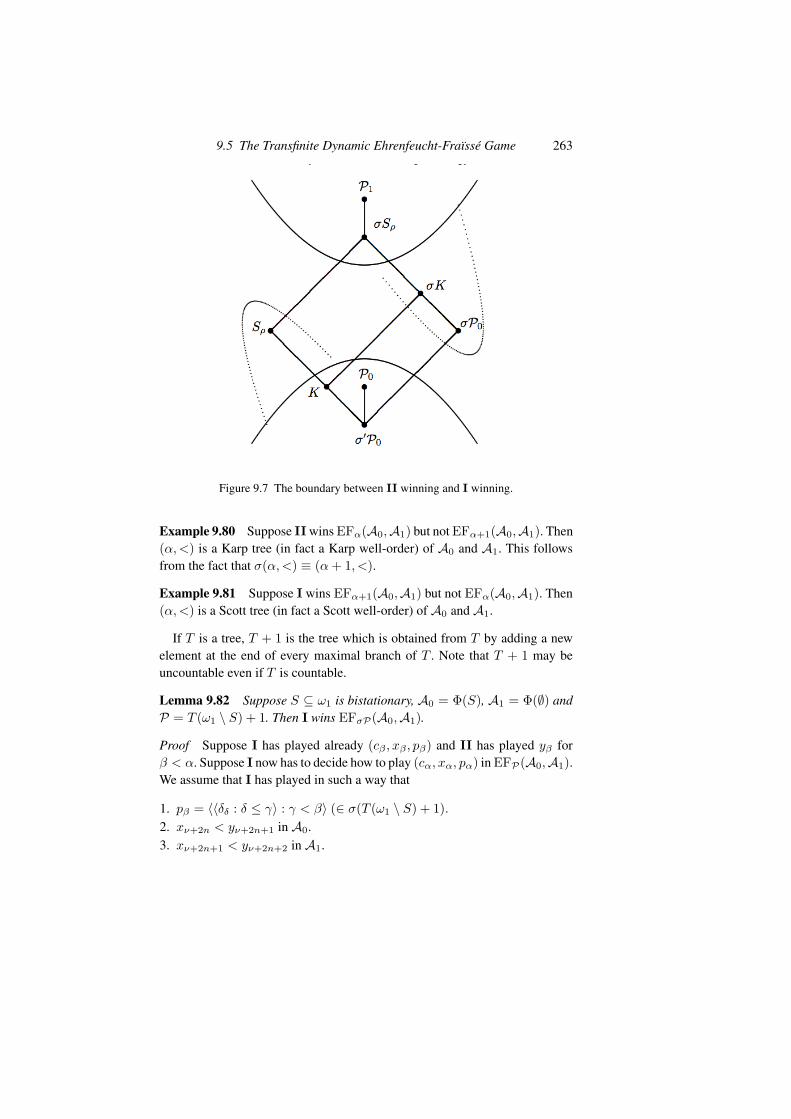
9.5 The Transfinite Dynamic Ehrenfeucht-Fraısse Game 263
Figure 9.7 The boundary between II winning and I winning.
Example 9.80 Suppose II wins EFα(A0,A1) but not EFα+1(A0,A1). Then(α, <) is a Karp tree (in fact a Karp well-order) of A0 and A1. This followsfrom the fact that σ(α, <) ≡ (α + 1, <).
Example 9.81 Suppose I wins EFα+1(A0,A1) but not EFα(A0,A1). Then(α, <) is a Scott tree (in fact a Scott well-order) of A0 and A1.
If T is a tree, T + 1 is the tree which is obtained from T by adding a newelement at the end of every maximal branch of T . Note that T + 1 may beuncountable even if T is countable.
Lemma 9.82 Suppose S ⊆ ω1 is bistationary, A0 = Φ(S), A1 = Φ(∅) andP = T (ω1 \ S) + 1. Then I wins EFσP(A0,A1).
Proof Suppose I has played already (cβ , xβ , pβ) and II has played yβ forβ < α. Suppose I now has to decide how to play (cα, xα, pα) in EFP(A0,A1).We assume that I has played in such a way that
1. pβ = ��δδ : δ ≤ γ� : γ < β� (∈ σ(T (ω1 \ S) + 1).2. xν+2n < yν+2n+1 in A0.3. xν+2n+1 < yν+2n+2 in A1.

Pages deleted for copyright reasons
1

270 Stronger Infinitary Logics
9.6 Topology of Uncountable Models
Countable models with countable vocabulary can be thought of as points inthe Baire space ωω. Likewise, models M of cardinality κ with vocabulary ofcardinality κ can be thought of as points fM in the set κκ. We can make κκ atopological space by letting the sets
N(f, α) = {g ∈ ωκ : f � α = g � α},
where α < κ, form the basis of the topology. Let us denote this general-ized Baire space κκ by Nκ. Now properties of models of size κ correspondto subsets of Nκ. In particular, modulo coding, isomorphism of structures ofcardinality κ becomes an “analytic” property in this space.
One of the basic questions about models of size κ that we can try to attackwith methods of logic is the question which of those models can be identifiedup to isomorphism by means of a set of invariants. Shelah’s Main Gap Theoremgives one answer: If M is any structure of cardinality κ ≥ ω1 in a countablevocabulary, then the first order theory of M is either of the two types:
Structure Case All uncountable models elementary equivalent to M can becharacterized in terms of dimension-like invariants.
Non-structure Case In every uncountable cardinality there are non-isomorphicmodels elementary equivalent toM that are extremely difficult to dis-tinguish from each other by means of invariants.
The game-theoretic methods we have developed in this book help us to an-alyze further the non-structure case. For this we need to develop some basictopology of Nκ. A set A ⊆ Nκ is dense if A meets every non-empty open set.The space Nκ has a dense subset of size κ<κ consisting of all eventually con-stant functions. If the Generalized Continuum Hypothesis GCH is assumed,then κ<κ = κ for all regular κ and κ<κ = κ+ for singular κ.
Theorem 9.87 (Baire Category Theorem) Suppose Aα, α < κ, are denseopen subsets of Nκ. Then
�α
Aα is dense.
Proof Let f0 ∈ Nκ and α0 < κ be arbitrary. If fξ and αξ for ξ < β havebeen defined so that
αζ < αξ and fξ ∈ N(fζ , αζ)
for ζ < ξ < β, then we define fβ and αβ as follows: Choose some g ∈ Nκ
such that g ∈ N(fξ, αξ) for all ξ < β and let αβ = supξ<β
αξ. Since Aβ
is dense, there is fβ ∈ Aβ ∩ N(g,αβ). When all fξ and αξ for ξ < κ have

9.6 Topology of Uncountable Models 271
been defined, we let f be such that f ∈ N(fξ, αξ) for all ξ < κ. Then f ∈�α
Aα ∩N(f0, α0).
Definition 9.88 A subset A of Nκ is said to be Σ11 (or analytic) if it is a
projection of a closed subset of Nκ × Nκ. A set is Π11 (or co-analytic) if its
complement is analytic. Finally, a set is ∆11 if it is both Σ1
1 and Π11.
Example 9.89 Examples of analytic sets relevant if κ is a regular cardinal> ω, are
CUBκ = {f ∈ Nκ : {α < κ : f(α) = 0} contains a club}
and
NSκ = {f ∈ Nκ : {α < κ : f(α) �= 0} contains a club}.
The set of α-sequences of elements of κ for various α < κ form a tree N<κ
under the subsequence relation. Any subset T of N<κ which is closed undersubsequences is called a tree in this section. A κ-branch of such a tree is anylinear subtree (branch) of height κ. Let us denote �g(β) : β < α� by g(α).
Lemma 9.90 A set A ⊆ Nκ is analytic iff there is a tree T ⊆ N<κ ×N<κ
such that for all f :
f ∈ A ⇐⇒ T (f) has a κ-branch, (9.7)
where T (f) = {g(α) : (g(α), f(α)) ∈ T}. Such a tree is called a tree repre-sentation of A.
Proof Suppose first A is analytic and B ⊆ κκ × κκ is a closed set such that
f ∈ A ⇐⇒ ∃g((f, g) ∈ B).
Let
T = {(f(α), g(α)) : (f, g) ∈ B,α < κ}.
Clearly now f ∈ A if and only if T (f) has a κ-branch. Conversely, supposesuch a T exists. Let B be the set of (f, g) such that (f(α), g(α)) ∈ T for allα < κ. The set B is closed and its projection is A.
Respectively, a set is co-analytic if and only if there is a tree T ⊆ N<κ ×N<κ such that for all f :
f ∈ A ⇐⇒ T (f) has no κ-branches, (9.8)
Let Tκ denote the class of all trees without κ-branches. Let Tλ,κ denote theset of subtrees of λ<κ of cardinality ≤ λ without any κ-branches.
272 Stronger Infinitary Logics
Proposition 9.91 Suppose B is a co-analytic subset of Nκ and T is as in(9.8). For any tree S ∈ Tκ let
BS = {f ∈ B : T (f) ≤ S}.
Then
B =�
S∈Tλ,κ
BS ,
where λ = κ<κ.
Proof Clearly BS ⊆ B if S ∈ Tκ. Conversely, suppose f ∈ B. Then ofcourse f ∈ BT (f). It remains to observe that |T (f)| ≤ κ<κ.
Suppose A ⊆ B is analytic and S is a tree as in (9.7). Let
T � = {(f(α), g(α), h(α)) : g(α) ∈ T (f), h(α) ∈ S(f)}. (9.9)
Note that |T �| ≤ κ<κ and T � has no κ-branches, for such a branch would giverise to a triple (f, g, h) which would satisfy f ∈ A\B. Note also that if f ∈ A,then there is a κ-branch {h(α) : α < κ} in S(f), and hence the mapping
g(α) �→ (f(α), g(α), h(α))
witnesses
T (f) ≤ T �.
We have proved:
Proposition 9.92 (Covering Theorem for Nκ) Suppose B is a co-analyticsubset of Nκ and S is as in (9.8). Suppose A ⊆ B is analytic. Then
A ⊆ BT
for some T ∈ Tλ,κ, where λ = κ<κ.
The idea is that the sets BT , T ∈ Tλ,κ cover the co-analytic set B com-pletely, and moreover any analytic subset of B can be already covered by asingle BT . Especially if B happens to be ∆1
1, then there is T ∈ Tλ,κ such thatB = BT .
Corollary (Souslin-Kleene Theorem for Nκ) Suppose B is a ∆11 subset of
Nκ. Then
B = BT
for some T ∈ Tλ,κ, where λ = κ<κ.
9.6 Topology of Uncountable Models 273
Corollary (Luzin Separation Theorem forNκ) Suppose A and B are disjointanalytic subsets of Nκ. Then there is a set of the form CT for some co-analyticset C and some T ∈ Tλ,κ, where λ = κ<κ, that separates A and B, i.e. A ⊆ Cand C ∩B = ∅.
In the case of classical descriptive set theory, which corresponds to assumingκ = ω, the sets BT are Borel sets. If we assume CH, then CUB and NS cannotbe separated by a Borel set.
Proposition 9.93 If κ<κ = κ, then the sets BT are analytic. If in addition Tis a strong bottleneck, then BT is ∆1
1.
Let us call a family B of elements of Tλ,κ universal if for every T ∈ Tthere is some S ∈ B such that T ≤ S. If Tλ,κ has a universal family of sizeµ, and κ<κ = κ, then by the above results every co-analytic set in Nκ is theunion of µ analytic sets. By results in [MV93] it is consistent relative to theconsistency of ZFC that Tκ+ , 2κ = κ+, has a universal family of size κ++
while 2κ+
= κ+++.
Definition 9.94 The class of Borel subsets of Nκ is the smallest class con-taining the open sets and the closed sets which is closed under unions andintersections of length κ.
Note that every closed set in Nκ is the union of κ<κ open sets (Exer-cise 9.57). So if κ<κ = κ, then the definition of Borelness can be simplified.
Theorem 9.95 Assume κ<κ = κ > ω. Then Nκ has two disjoint analyticsets that cannot be separated by Borel sets.
Proof Note that κ is a regular cardinal. Every Borel set A has a “Borel code”c such that A = Bc. Let us suppose A = Bc separates the disjoint analyticsets CUBκ and NSκ defined in Example 9.89. For example, CUB ⊆ A andA ∩ NSκ = ∅. Let P = (2<κ,≤) be the Cohen forcing for adding a genericsubset for κ. Let G be P-generic and g =
�P . Now either g ∈ A or g /∈ A.
Let us assume, w.l.o.g., that g ∈ A. Let p � g ∈ Bc. Let M ≺ (H(µ),∈, <∗)for a large µ such that κ, p,P, TC(c) ∈ M , M<κ ⊆ M , and <∗ is a well-order of H(µ). Since κ<κ = κ > ω, we may also assume |M | = κ. Since Pis < κ-closed, it is easy to construct a P-generic G� over M in V such that
{α < κ : M |= “(g)G�(α) �= 0”} contains a club. (9.10)
It is easy to show that Bc = (Bc)G� . Since
M |= “p � g ∈ Bc”,
whence (g)G� ∈ Bc and therefore (g)G� /∈ NSκ. This contradicts (9.10).
274 Stronger Infinitary Logics
Example 9.96 Suppose M is a structure with M = κ. We call the analyticset
{N : N = κ and N ∼= M}
the orbit of M. Let N �∼= M. Now player I has an obvious winning strategyρ in EFκ(M,N ): he simply makes sure that all elements of both models areplayed. Obviously there are many ways to play all the elements but any ofthem will do. Let us consider the co-anaytic set B = {fN : N = κ and N �∼=M}. Let S(N ) be the Scott tree Sρ of the pair (M,N ). Let us choose a treerepresentation T of B in such a way that for all N with N = κ, T (fN ) =S(N ). If now fN ∈ BT � , then player I wins EFT �(M,N ).
Recall that ifM is a countable structure and α is the Scott height ofM, thenI wins EFDα+ω(M,N ) wheneverM �∼= N and N is countable. Equivalently,using the notation of Example 9.54, player I wins EFBα+ω (M,N ) wheneverM �∼= N and N is countable. We now generalize this property of Bα+ω touncountable structures.
Definition 9.97 Suppose κ is an infinite cardinal and M is a structure ofcardinality κ. A tree T is a universal Scott tree of a structure M if T has nobranches of length κ and player I wins EFσT (M,N ) whenever M �∼= N and|N | = |M |.
The idea of the universal Scott tree is that the tree T alone suffices as a clockfor player I to win all the 2κ different games EFT (M,N ) where M �∼= N and|N | = |M |. Universal Scott trees exist: there is always a universal Scott treeof cardinality ≤ 2κ as we can put the various Scott trees of the pairs (M,N ),M �∼= N , |M | = |N |, each of them of the size ≤ κ<κ, together into one tree.So the question is: How small universal Scott trees does a given structure have?
If κ<κ = λ and Tλ,κ has a universal family of size µ, then every structureof size κ has a universal Scott tree of size µ.
If we allowed T to have a branch of length κ, any such tree would be auniversal Scott tree of any structure of cardinality κ.
We ask whether I wins EFσT (M,N ) rather than in EFT (M,N ) in orderto preserve the analogy with the concept of a Scott tree. A universal Scott treeT in our sense would give rise to a universal Scott tree σT in the latter sense.Note that |σT | = |T |<κ, so this is the order of magnitude of a difference in thesize of universal Scott trees in the two possible definitions.
Proposition 9.98 Suppose κ<κ = κ and M is a structure with M = κ. thefollowing are equivalent:
(1) The orbit of M is ∆11.

9.7 Historical Remarks and References 275
(2) M has a universal Scott tree of cardinality κ.
Proof Suppose first (2) is true. Then
M �∼= N ⇐⇒ player I wins EFσT (M,N ).
The existence of a winning strategy of I can be written in Π11 form since we as-
sume κ<κ = κ. Assume then (1). Let ρ be a strategy of player I in EFκ(M,N )in which he simply enumerates the universes. Note that this is independent ofN . Let S(N ) be the Scott tree Sρ of the pair (M,N ). Let us consider theco-anaytic set B = {fN : N = κ and N �∼= M}. Let us choose a tree rep-resentation T of B as in Example 9.96. If now fN ∈ BT � , then player I winsEFT �(M,N ). By the above Souslin-Kleene theorem, (1) implies the existenceof a tree T � such that B = B�
T. Thus for any N with N = κ, M �∼= N im-
plies that player I wins EFT �(M,N ). Thus T � is a universal Scott tree of M.Moreover, |T �| = κ<κ = κ.
The question whether the orbit of M is ∆11 is actually highly connected
to stability-theoretic properties of the first order theory of M, see [HT91] formore on this.
9.7 Historical Remarks and References
Excellent sources for stronger infinitary languages are the textbook [Dic75],the handbook chapter [Dic85] and the book chapter [Kue75]. The Ehrenfucht-Fraısse game for the logics L∞λ appeared in [Ben69] and [Cal72]. Propo-sition 9.32, Proposition 9.45 and the corollary of Proposition 9.45 are dueto Chang [Cha68]. The concept of Definition 9.40 and its basic propertieswere isolated independently by Dickmann [Dic75] and Kueker [Kue75]. The-orem 9.31 is from [She78].
Looking at the origins of the transfinite Ehrenfeucht-Fraısse Game, one canobserve that the game plays a role in [She78], and is then systematically stud-ied, first in the framework of back-and-forth sets in [Kar84], and then explicitlyas a game in [Hyt87], [Hyt90], [HV90] and [Oik90].
The importance of trees in the study of the transfinite Ehrenfeucht-FraısseGame was first recognized in [Kar84] and [Hyt87]. The crucial property oftrees, or more generally partial orders, is Lemma 9.55 part (ii), which goesback to Kurepa [Kur56]. A more systematic study of the quasi-order P ≤ P �of partial orders, with applications to games in mind, was started in [HV90],where Lemma 9.57, Definition 9.58, Lemma 9.59 and Lemma 9.60 originate.The important role of the concept of persistency (Definition 9.63) gradually
276 Stronger Infinitary Logics
emerged and was explicitly isolated and exploited in [Huu95]. Once it be-came clear that trees may be incomparable by ≤, the concept of bottleneckarose quite naturally. Definition 9.64 is from [TV99]. The relative consistencyof the non-existence of non-trivial bottlenecks (Theorem 9.65) was proved in[MV93]. For more on the structure of trees see [TV99] and [DV04].
The point of studying trees in connection with the transfinite Ehrenfeucht-Fraısse Game is that there are two very natural tree structures behind the game.The first tree that arises from the game is the tree of sequences of moves, as inLemma 9.73. This tree originates in [Kar84]. The second, and in a sense morepowerful tree is the tree of strategies of a player, as in Definition 9.69 and thesubsequent Proposition 9.71. This idea originates from [Hyt87].
The “transfinite” analogues of Scott ranks are the Scott and Karp trees, in-troduced in [HV90]. Because of problems of incomparability of some trees,the picture of the “Scott watershed” is much more complicated than in the caseof games of length ω, as one can see by comparing Figure 7.4 and Figure 9.7.Proposition 9.85 and Theorem 9.86 are from [Tuu90].
There is a form of infinitary logic the elementary equivalence of which cor-responds exactly to the existence of winning strategy for II in EFα, in thespirit of the Strategic Balance of Logic. These infinitary logics are called in-finitely deep languages. Their formulas are like formulas of Lκλ but there areinfinite descending chains of subformulas. Thus, if we think of the syntax ofa formula as a tree, the tree may have transfinite rank. These languages wereintroduced in [HR76] and studied in [Kar79], [Ran81], [Kar84], [Hyt90] and[Tuu92]. See [Vaa95] for a survey on the topic.
There is also a transfinite version of the Model Existence Game, the otherleg of the Strategic Balance of Logic, with applications to undefinability of(generalized) well-order and Separation Theorems, see [Tuu92] and [Oik97].
It was recognized already in [She78] that the roots of the problem of extend-ing the Scott Isomorphism Theorem to uncountable cardinalities lie in stabilitytheoretic properties of the models in question. This was made explicit in thecontext of transfinite Ehrenfeucht-Fraısse Games in [HT91]. It turns out thatthere is indeed a close connection between the structure of Scott and Karptrees of elementary equivalent uncountable models and the stability theoreticproperties such as superstability, DOP and OTOP, of the (common) first ordertheory. For more on this, see [Hyt92], [HST93], and [HS99].
A good testing field for the power of long Ehrenfeucht-Fraısse games turnedout to be the area of almost free groups, where it seemed that the applicabilityof the infinitary languages Lκλ had been exhausted. For results in this direc-tion, see [MO93], [EFS95], [SV02] and [Vai03].
An alternative to considering transfinite Ehrenfeucht-Fraısse Games is to

Exercises 277
study isomorphism in a forcing extension. Isomorphism in a forcing exten-sion is called potential isomorphism. The basic reference is [NS78]. See also[HHR04].
Early on it was recognized that the trees T (S) (see Example 9.61) are veryuseful and in some sense fundamental in the area of transfinite Ehrenfeucht-Fraısse Games. The question arose, whether there is a largest such tree forS ⊆ ω1 bistationary. Quite unexpectedly the existence of a largest such treeturned out to be consistent relative to the consistency of ZF. The name “Canarytrees” was coined for them, because such a tree would indicate whether somestationary set was killed. See [MS93] and [HR01] for results on the Canarytree.
While the Ehrenfeucht-Fraısse game of length ω is almost trivially deter-mined, the Ehrenfeucht-Fraısse game of length ω1 (and also of length ω + 1)can be non-determined, see [Hyt92], [MSV93] and [HSV02]. This has devas-tating consequences for attempts to use transfinite Ehrenfeucht-Fraısse gamesto classify uncountable models. It is a phenomenon closely related to the in-comparability of non-well-founded trees by the relation≤. This non-determin-ism is ultimately also the reason why the simple picture Figure 7.4 becomesFigure 9.7.
Some of the complexities of uncountable models can be located alreadyon the topological level, as is revealed by the study of the spaces Nκ. Thesespaces were studied under the name of κ-metric spaces in [Sik50], [JW78]and [Tod81b]. Their role as spaces of models, in the spirit of [Vau73], wasemphasized in [MV93]. For more on the topology of uncountable models, see[Vaa91], [Vaa95] and [SV00]. See [Vaa08] for an informal exposition of somebasic ideas. Theorem 9.95 is from [SV00].
Exercise 9.22 is from [NS78]. Exercises 9.29 and 9.30 are from [Hyt87].Exercise 9.35 is from [HV90]. Exercise 9.40 is from [Kur56]. Exercise 9.41 isfrom [Huu95]. Exercise 9.47 is from [Tod81a]. Exercise 9.56 is due to LauriHella.
Exercises
9.1 Show that player II wins EFℵ0ω
(M,M�) if and only if she has a winningstrategy in EFω(M,M�).
9.2 Show that I wins EFDω12 (M,N ) if M = (Q, <) and N = (R, <).
9.3 Show that in Example 9.2 player I has a winning strategy already inEFDω1
2 (M,M�).9.4 Show that M �p N , where M and N are as in Example 9.4.

Pages deleted for copyright reasons
1
10Generalized Quantifiers
10.1 Introduction
First order logic is not able to express “there exists infinitely many x such that...” nor “there exists uncountably many x such that ...”. Also, if we restrict our-selves to finite models, first order logic is not able to express “there exists aneven number of x such that ...”. These are examples of new logical operationscalled generalized quantifiers. There are many others, such as the Magidor-Malitz quantifiers, cofinality quantifiers, stationary logic, and so on. We canextend first order logic by adding such new quantifiers. In the case of “thereexists infinitely many x such that ...” the resulting logic is not axiomatizable,but in the case of “there exists uncountably many x such that ...” the new logicis indeed axiomatizable. The proof of the completeness theorem for this quan-tifier is non-trivial going well beyond the Completeness Theorem of first orderlogic.

284 Generalized Quantifiers
10.2 Generalized Quantifiers
Generalized quantifiers occur everywhere in our language. Here are some ex-amples:
Two thirds voted for JohnExactly half remains.Most wanted to leave.Some but not all liked it.Between 10% and 20% were students.Hardly anybody touched the cake.The number of white balls is even.There are infinitely many primes.There are uncountably many reals.
These are instances of generalized quantifiers in natural language1. The math-ematical study of quantifiers provides an exact framework in which such quan-tifiers can be investigated. An overall goal is to find invariants for such objects,that is, to classify them and find the characteristic properties of quantifiers ineach class. Typical questions that we study are: which quantifier is “definable”in terms of another given quantifier, which quantifiers can be axiomatized,which satisfy the Compactness Theorem, etc. We start with a very generalconcept of a quantifier and then later we impose restrictions. Usually in theliterature the generalized quantifiers are assumed to be what we call bijectionclosed (see Definition 10.16).
Definition 10.1 A weak (generalized) quantifier is a mapping Q which mapsevery non-empty set A to a subset of P(A). A weak (generalized) quantifieron a domain A is any subset of P(A).
Virtually all quantifiers we consider are quantifiers in the first sense, i.e.mappings A �−→ Q(A). However, most actual results and examples are abouta fixed given domain A, whence the concept of a quantifier on a domain. Thedomain is assumed to be a set.
The set-theoretic nature of a quantifier (as a mapping) is somewhat problem-atic. We cannot call a quantifier a function in the set-theoretical sense since itsdomain consists of all possible non-empty sets. However, this problem does notarise in practice. Our quantifiers are in general definable so we can treat themas classes. If we have to talk about all quantifiers, definable or not, we haveto restrict ourselves to considering domains A contained in one sufficiently1 Quantifiers occurring in natural language are usually of a slightly more complex form, such as
“Two thirds of the people voted for John”, “Exactly half of the cake remains”, “Most studentswanted to leave”, “Some but not all viewers liked it”.
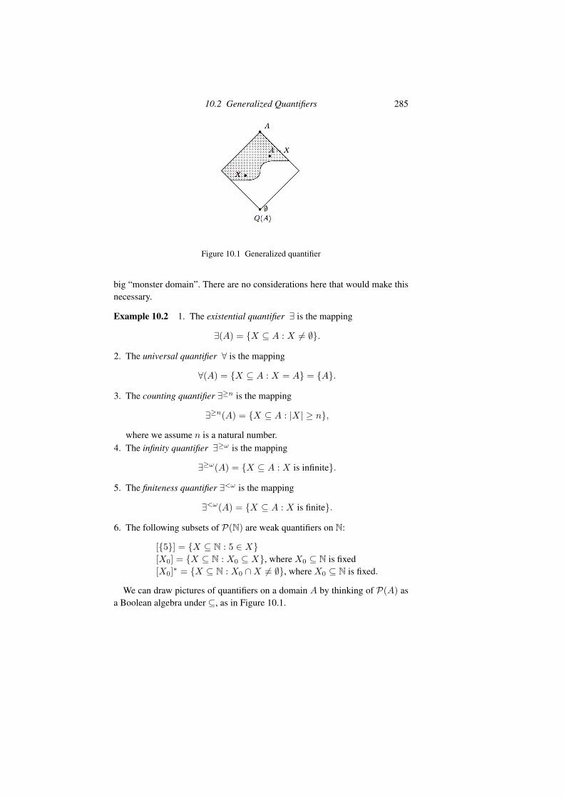
10.2 Generalized Quantifiers 285
Figure 10.1 Generalized quantifier
big “monster domain”. There are no considerations here that would make thisnecessary.
Example 10.2 1. The existential quantifier ∃ is the mapping
∃(A) = {X ⊆ A : X �= ∅}.
2. The universal quantifier ∀ is the mapping
∀(A) = {X ⊆ A : X = A} = {A}.
3. The counting quantifier ∃≥n is the mapping
∃≥n(A) = {X ⊆ A : |X| ≥ n},
where we assume n is a natural number.4. The infinity quantifier ∃≥ω is the mapping
∃≥ω(A) = {X ⊆ A : X is infinite}.
5. The finiteness quantifier ∃<ω is the mapping
∃<ω(A) = {X ⊆ A : X is finite}.
6. The following subsets of P(N) are weak quantifiers on N:
[{5}] = {X ⊆ N : 5 ∈ X}[X0] = {X ⊆ N : X0 ⊆ X}, where X0 ⊆ N is fixed[X0]∗ = {X ⊆ N : X0 ∩X �= ∅}, where X0 ⊆ N is fixed.
We can draw pictures of quantifiers on a domain A by thinking of P(A) asa Boolean algebra under ⊆, as in Figure 10.1.
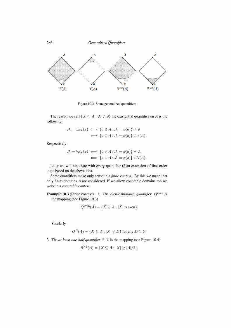
286 Generalized Quantifiers
Figure 10.2 Some generalized quantifiers
The reason we call {X ⊆ A : X �= ∅} the existential quantifier on A is thefollowing:
A |= ∃xϕ(x) ⇐⇒ {a ∈ A : A |= ϕ(a)} �= ∅⇐⇒ {a ∈ A : A |= ϕ(a)} ∈ ∃(A).
Respectively
A |= ∀xϕ(x) ⇐⇒ {a ∈ A : A |= ϕ(a)} = A
⇐⇒ {a ∈ A : A |= ϕ(a)} ∈ ∀(A).
Later we will associate with every quantifier Q an extension of first orderlogic based on the above idea.
Some quantifiers make only sense in a finite context. By this we mean thatonly finite domains A are considered. If we allow countable domains too wework in a countable context.
Example 10.3 (Finite context) 1. The even-cardinality quantifier Qeven isthe mapping (see Figure 10.3)
Qeven(A) = {X ⊆ A : |X| is even}.
Similarly
QD(A) = {X ⊆ A : |X| ∈ D} for any D ⊆ N.
2. The at-least-one-half quantifier ∃≥ 12 is the mapping (see Figure 10.4)
∃≥ 12 (A) = {X ⊆ A : |X| ≥ |A|/2}.
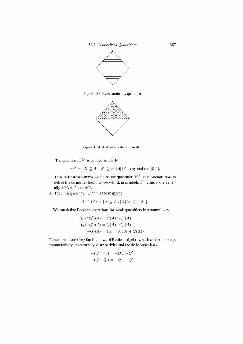
10.2 Generalized Quantifiers 287
Figure 10.3 Even cardinality quantifier
Figure 10.4 At-least-one-half quantifier
The quantifier ∃≥r is defined similarly
∃≥r = {X ⊆ A : |X| ≥ r · |A|} for any real r ∈ [0, 1].
Thus at-least-two-thirds would be the quantifier ∃≥ 23 . It is obvious how to
define the quantifier less-than-two-third, in symbols ∃<23 , and more gener-
ally ∃<r, ∃≤r and ∃>r.3. The most quantifier ∃most is the mapping
∃most(A) = {X ⊆ A : |X| > |A−X|}.
We can define Boolean operations for weak quantifiers in a natural way:
(Q ∩Q�)(A) = Q(A) ∩Q�(A)(Q ∪Q�)(A) = Q(A) ∪Q�(A)
(−Q)(A) = {X ⊆ A : X /∈ Q(A)}.
These operations obey familiar laws of Boolean algebras, such as idempotency,commutativity, associativity, distributivity and the de Morgan laws:
−(Q ∩Q�) = −Q ∪ −Q�
−(Q ∪Q�) = −Q ∩ −Q�.
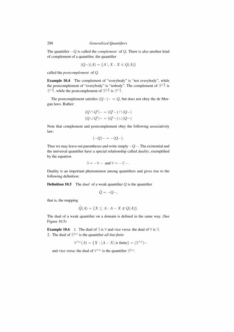
288 Generalized Quantifiers
The quantifier −Q is called the complement of Q. There is also another kindof complement of a quantifier, the quantifier
(Q−)(A) = {A \X : X ∈ Q(A)}
called the postcomplement of Q.
Example 10.4 The complement of “everybody” is “not everybody”, whilethe postcomplement of “everybody” is “nobody”. The complement of ∃≥ 2
3 is∃<
23 , while the postcomplement of ∃≥ 2
3 is ∃<13 .
The postcomplement satisfies (Q−)− = Q, but does not obey the de Mor-gan laws. Rather:
(Q ∩Q�)− = (Q�−) ∩ (Q−)(Q ∪Q�)− = (Q�−) ∪ (Q−)
Note that complement and postcomplement obey the following associativitylaw:
(−Q)− = −(Q−).
Thus we may leave out parentheses and write simply−Q−. The existential andthe universal quantifier have a special relationship called duality, exemplifiedby the equation
∃ = −∀ − and ∀ = −∃ − .
Duality is an important phenomenon among quantifiers and gives rise to thefollowing definition:
Definition 10.5 The dual of a weak quantifier Q is the quantifier
Q = −Q−,
that is, the mapping
Q(A) = {X ⊆ A : A−X �∈ Q(A)}.
The dual of a weak quantifier on a domain is defined in the same way. (SeeFigure 10.5)
Example 10.6 1. The dual of ∃ is ∀ and vice versa: the dual of ∀ is ∃.2. The dual of ∃≥ω is the quantifier all-but-finite
∀<ω(A) = {X : |A−X| is finite} = (∃<ω)−
and vice versa: the dual of ∀<ω is the quantifier ∃≥ω.

Pages deleted for copyright reasons
1
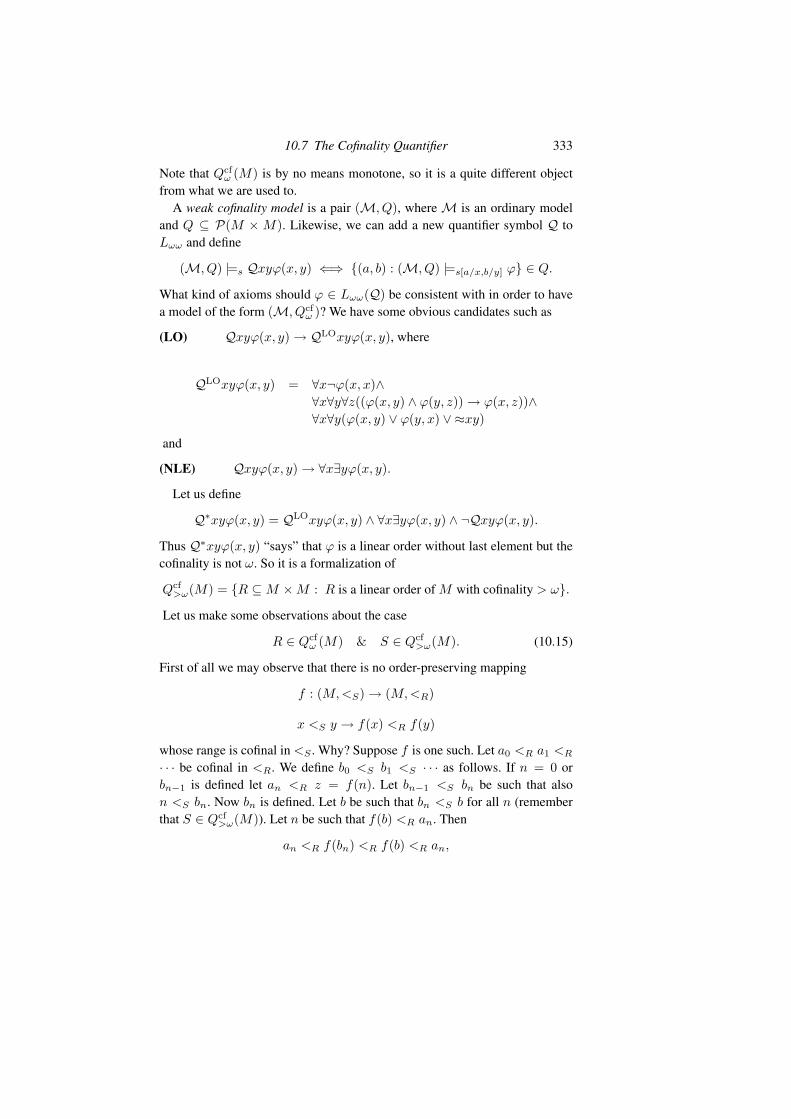
10.7 The Cofinality Quantifier 333
Note that Qcfω
(M) is by no means monotone, so it is a quite different objectfrom what we are used to.
A weak cofinality model is a pair (M, Q), where M is an ordinary modeland Q ⊆ P(M × M). Likewise, we can add a new quantifier symbol Q toLωω and define
(M, Q) |=s Qxyϕ(x, y) ⇐⇒ {(a, b) : (M, Q) |=s[a/x,b/y] ϕ} ∈ Q.
What kind of axioms should ϕ ∈ Lωω(Q) be consistent with in order to havea model of the form (M, Qcf
ω)? We have some obvious candidates such as
(LO) Qxyϕ(x, y) → QLOxyϕ(x, y), where
QLOxyϕ(x, y) = ∀x¬ϕ(x, x)∧∀x∀y∀z((ϕ(x, y) ∧ ϕ(y, z)) → ϕ(x, z))∧∀x∀y(ϕ(x, y) ∨ ϕ(y, x) ∨ ≈xy)
and
(NLE) Qxyϕ(x, y) → ∀x∃yϕ(x, y).
Let us define
Q∗xyϕ(x, y) = QLOxyϕ(x, y) ∧ ∀x∃yϕ(x, y) ∧ ¬Qxyϕ(x, y).
Thus Q∗xyϕ(x, y) “says” that ϕ is a linear order without last element but thecofinality is not ω. So it is a formalization of
Qcf>ω
(M) = {R ⊆ M ×M : R is a linear order of M with cofinality > ω}.
Let us make some observations about the case
R ∈ Qcfω
(M) & S ∈ Qcf>ω
(M). (10.15)
First of all we may observe that there is no order-preserving mapping
f : (M, <S) → (M, <R)
x <S y → f(x) <R f(y)
whose range is cofinal in <S . Why? Suppose f is one such. Let a0 <R a1 <R
· · · be cofinal in <R. We define b0 <S b1 <S · · · as follows. If n = 0 orbn−1 is defined let an <R z = f(n). Let bn−1 <S bn be such that alson <S bn. Now bn is defined. Let b be such that bn <S b for all n (rememberthat S ∈ Qcf
>ω(M)). Let n be such that f(b) <R an. Then
an <R f(bn) <R f(b) <R an,
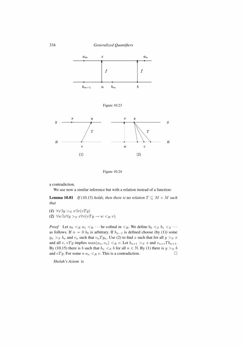
334 Generalized Quantifiers
Figure 10.23
Figure 10.24
a contradiction.We use now a similar inference but with a relation instead of a function:
Lemma 10.81 If (10.15) holds, then there is no relation T ⊆ M ×M suchthat
(1) ∀x∃y >S x∃v(vTy)(2) ∀w∃x∀y >S x∀v(vTy → w <R v).
Proof Let a0 <R a1 <R · · · be cofinal in <R. We define b0 <S b1 <S · · ·as follows. If n = 0 b0 is arbitrary. If bn−1 is defined choose (by (1)) someyn >S bn and vn such that vnTyn. Use (2) to find x such that for all y >S xand all v, vTy implies max(an, vn) <R v. Let bn+1 >S x and vn+1Tbn+1.By (10.15) there is b such that bn <S b for all n ∈ N. By (1) there is y >S band vTy. For some n an <R v. This is a contradiction.
Shelah’s Axiom is
336 Generalized Quantifiers
I II Explanation
Qxyϕ(x, y) a played formula
QLOxyϕ(x, y)∧∀x∃yϕ(x, y)
Q∗xyϕ(x, y) a played formula
QLOxyϕ(x, y)∧∀x∃yϕ(x, y)
Qxyϕ(x, y) playedQ∗xyψ(x, y) formulas
ϕ(c, d)¬ψ(c, d)
or¬ϕ(c, d)ψ(c, d)
ϕ ∨ ¬ϕ ϕ any sentence
ϕ or¬ϕ
Theorem 10.83 (Model Existence Theorem for Cofinality Logic) Suppose Lis a vocabulary of cardinality ≤ κ and T is a set of L-sentences of Lωω(Q).TFAE
(1) T has a model (M, Q) satisfying (LO)+(NLE).(2) Player II has a winning strategy in MEGQ,cf
κ(T,L).
Proof If (M, Q) |= (T) + (LO) +(NLE), then clearly (2) holds. Conversely,suppose (2) holds. We let Player I play the obvious enumeration strategy. LetH be the set of responses of II, using her winning strategy. By construction,H gives rise to a model of (T) + (LO) +(NLE). Now the details: Let H be theset of responses of II, using her winning strategy, to a maximal play of I. LetM be defined from H as before. We define a weak cofinality quantifier Q onM as follows:
Q = {{([c], [d]) : ϕ(c, d) ∈ H} : Qxyϕ(x, y) ∈ H}.
Now we show (M, Q) |= T by proving the following claim. By our previouswork we have

10.7 The Cofinality Quantifier 337
1. ≈tt ∈ H2. If ϕ(c) ∈ H and ≈ct ∈ H then ϕ(t) ∈ H3. If ϕ ∧ ψ ∈ H , then ϕ ∈ H and ψ ∈ H4. If ϕ ∨ ψ ∈ H , then ϕ ∈ H and ψ ∈ H5. If ∀xϕ(x) ∈ H , then ϕ(c) ∈ H for all c ∈ C6. If ∃xϕ(x) ∈ H , then ϕ(c) ∈ H for some c ∈ C.
Now we can note further
7. If ϕ �∈ H , then ¬ϕ ∈ H (¬ϕ has to be written in NNF).
The reason for 7 is simply that I can play ϕ ∨ ¬ϕ whenever he wants.
Claim
ϕ ∈ H ⇐⇒ M |= ϕ
Proof Note that:
• If ϕ ∈ H and ψ ∈ H , then ϕ ∧ ψ ∈ H for otherwise ¬(ϕ ∧ ψ) ∈ Hwhence ¬ϕ ∈ H or ¬ψ ∈ H . This is not possible as then M |= ϕ ∧ ¬ϕ orM |= ψ ∧ ¬ψ.
• If ϕ ∈ H or ψ ∈ H , then ϕ ∨ ψ ∈ H for otherwise ¬ϕ ∈ H and ¬ψ ∈ H .• If ϕ(c) ∈ H for all c ∈ C, then ∀xϕ(x) ∈ H for otherwise ¬∀xϕ(x),
which in NNF is ∃x¬ϕ(x) is in H , leading to the conclusion that M |=ϕ(c) ∧ ¬ϕ(c) for some c.
• If ϕ(c) ∈ H for some c ∈ C, then ∃xϕ(x) ∈ H for otherwise ¬∃xϕ(x) ∈H , leading to a contradiction.
• If Qxyϕ(x, y) ∈ H , then M |= Qxyϕ(x, y), for let R = {([c], [d]) : M |=ϕ(c, d)}. By the induction hypothesis
R = {([c], [d]) : ϕ(c, d) ∈ H}.
By construction, R ∈ Q(M).• If Q∗xyϕ(x, y) ∈ H , then M |= Q∗xyϕ(x, y), for let R = {([c], [d]) :
M |= ϕ(c, d)}. As above, R = {([c], [d]) : ϕ(c, d) ∈ H}. By construction,R is a linear order without last element. If M |= Qxyϕ(x, y), then R ={([c], [d]) : ψ(c, d) ∈ H} for some ψ such that Qxyψ(x, y) ∈ H . By therules of the game, there are c and d such that ϕ(c, d) ∈ H � ψ(c, d) ∈ H ,contrary to the choice of ψ.
• If M |= Qxyϕ(x, y) then Qxyϕ(x, y) ∈ H , for otherwise ¬Qxyϕ(x, y) ∈H . By induction hypothesis, M |= Qxyϕ(x, y) implies
R = {([c], [d]) : ϕ(c, d) ∈ H}= {([c], [d]) : M |= ϕ(c, d)}

338 Generalized Quantifiers
is a linear order without last element and QLOxyϕ(x, y) ∧ ∀x∃yϕ(x, y) ∈H . IfQ∗xyϕ(x, y) ∈ H , 9 leads to a contradiction. Hence ¬Q∗xyϕ(x, y) ∈H , whence Qxyϕ(x, y) ∈ H .
• If M |= Q∗xyϕ(x, y), thenQ∗xyϕ(x, y) ∈ H , for otherwise¬Q∗xyϕ(x, y) ∈H . Since QLOxyϕ(x, y) ∧ ∀x∃yϕ(x, y) ∈ H , we have Qxyϕ(x, y) ∈ H .By 8, M |= Qxyϕ(x, y), a contradiction.
Theorem 10.84 (Weak Compactness of Cofinality Logic) If T is a set of sen-tences of Lωω(Q) and every finite subset has a weak cofinality model satisfying(LO) + (NLE), then so does the whole T .
Proof As in Theorem 10.63.
Theorem 10.85 (Weak Omitting Types Theorem of Cofinality Logic) As-sume κ is an infinite cardinal. Let L be a vocabulary of cardinality ≤ κ, Tan Lωω(Q)-theory and for each ξ < κ, Γξ is a set {ϕξ
α(x) : α < κ} of
Lωω(Q)-formulas in the vocabulary L. Assume that
1. If α ≤ β < κ, then T � ϕξ
β(x) → ϕξ
α(x).
2. For every Lωω(Q)-formula ψ(x), for which T ∪ {ψ(x)} is consistent, andfor every ξ < κ, there is an α < κ such that T ∪ {ψ(x)} ∪ {¬ϕξ
α(x)} is
consistent.
Then T has a weak cofinality model which omits Γ.
Proof As in Theorem 6.62.
Definition 10.86 The union of an elementary chain (Mα, Qα) of weak cofi-nality models of (LO) + (NLE) is (M, Q), where M =
�αMα and
Q = {R ⊆ M ×M : R is a linear order without last element andthere is α < κ such that R ∩ (Mβ ×Mβ) ∈ Qβ for all β ≥ α}.
Lemma 10.87 (Union Lemma) The union of an elementary chain is an ele-mentary extension of each member of the chain.
Proof We will do only the case of Qxyϕ(x, y). Suppose first (M, Q) |=s
Qxyψ(x, y), where s is an assignment into Mα. Then R ∈ Q where for a, b ∈M
aRb ←→ (M, Q) |=s[a/x,b/y] ψ(x, y).
By definition there is β ≥ α such that R ∩ (Mγ ×Mγ) ∈ Qγ for γ ≥ β. Bythe induction hypothesis, for a, b ∈ Mγ
aRb ←→ (Mγ , Qγ) |=s[a/x,b/y] ψ(x, y).

10.7 The Cofinality Quantifier 339
i.e.
(Mγ , Qγ) |=s Qxyψ(x, y).
By assumption (Mα, Qα) |=s Qxyψ(x, y). Conversely, suppose (M, Q) �|=s
Qxyψ(x, y). Then for all β ≥ α: R ∩ (Mβ ×Mβ) /∈ Qβ where for a, b ∈ M
aRb ⇐⇒ (M, Q) |=s[a/x,b/y] ψ(x, y).
By the induction hypothesis for a, b ∈ Mβ
aRb ⇐⇒ (Mβ , Qβ) |=s[a/x,b/y] ψ(x, y)
i.e.
(Mβ , Qβ) �|=s Qxyϕ(x, y)
and hence (Mα, Qα) �|=s Qxyϕ(x, y).
Lemma 10.88 For every infinite weak cofinality model (M, Q) and everyκ ≥ |M | there is (M�, Q�) such that (M, Q) ≺ (M�, Q�) and every linearorder on M, which has no last element and which is Lωω(Q)-definable on Mwith parameters, has cofinality κ.
Proof See Exercise 10.109.
Lemma 10.89 (Main Lemma) Suppose (M, Q) is an infinite weak cofinalitymodel of (SA) and ϕ(x, y) is a formula of Lωω(Q) such that (M∗, Q) |=Qxyϕ(x, y). Then there is a weak cofinality model (M�, Q�) such that
(1) (M, Q) ≺ (M�, Q�)(2) For some b ∈ M � \M we have (M�, Q�) |= ϕ(a, b) for all a ∈ M(3) For every ψ(x, y) such that (M, Q) |= Q∗xyψ(x, y) and every d ∈ M �
we have (M�, Q�) |= ψ(d, a) for some a ∈ M .
Proof In the light of Lemma 10.88 may assume, without loss of generality,that the modelM and the vocabulary L have an infinite cardinality κ, and everylinear order on M which has no last element and which is Lωω(Q)-definableon M with parameters, has cofinality κ. Let c be a new constant symbol andT the theory
{θ : (M∗, Q) |= θ} ∪ {ϕ(a, c) : a ∈ M}.
The useful criterion, familiar from the proof of Lemma 10.78, is in this casevery simple:
T ∪ {θ(c)} is consistent iff (M∗, Q) |= ∀x∃y(ϕ(x, y) ∧ θ(y)). (10.16)
Proof of (10.16). Suppose (M∗, Q) |= ∀x∃y(ϕ(x, y) ∧ θ(y)). Let T0 ⊆ T
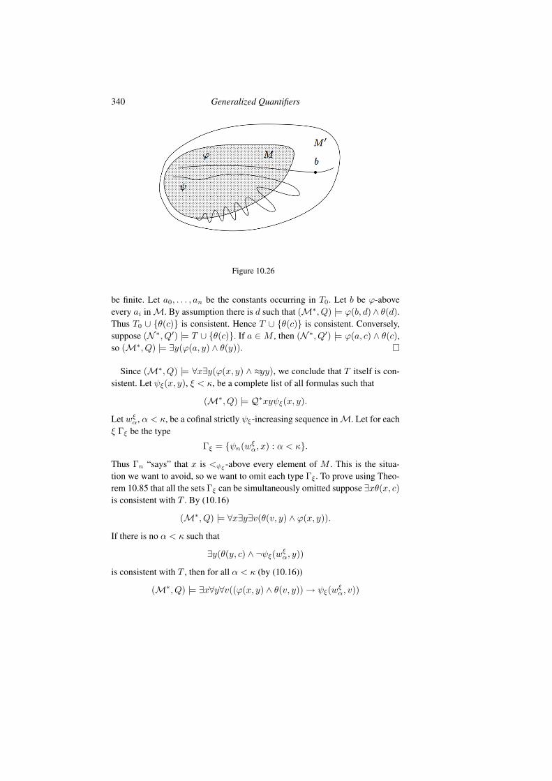
340 Generalized Quantifiers
Figure 10.26
be finite. Let a0, . . . , an be the constants occurring in T0. Let b be ϕ-aboveevery ai in M. By assumption there is d such that (M∗, Q) |= ϕ(b, d)∧ θ(d).Thus T0 ∪ {θ(c)} is consistent. Hence T ∪ {θ(c)} is consistent. Conversely,suppose (N ∗, Q�) |= T ∪ {θ(c)}. If a ∈ M , then (N ∗, Q�) |= ϕ(a, c) ∧ θ(c),so (M∗, Q) |= ∃y(ϕ(a, y) ∧ θ(y)).
Since (M∗, Q) |= ∀x∃y(ϕ(x, y) ∧ ≈yy), we conclude that T itself is con-sistent. Let ψξ(x, y), ξ < κ, be a complete list of all formulas such that
(M∗, Q) |= Q∗xyψξ(x, y).
Let wξ
α, α < κ, be a cofinal strictly ψξ-increasing sequence in M. Let for each
ξ Γξ be the type
Γξ = {ψn(wξ
α, x) : α < κ}.
Thus Γn “says” that x is <ψξ -above every element of M . This is the situa-tion we want to avoid, so we want to omit each type Γξ. To prove using Theo-rem 10.85 that all the sets Γξ can be simultaneously omitted suppose ∃xθ(x, c)is consistent with T . By (10.16)
(M∗, Q) |= ∀x∃y∃v(θ(v, y) ∧ ϕ(x, y)).
If there is no α < κ such that
∃y(θ(y, c) ∧ ¬ψξ(wξ
α, y))
is consistent with T , then for all α < κ (by (10.16))
(M∗, Q) |= ∃x∀y∀v((ϕ(x, y) ∧ θ(v, y)) → ψξ(wξ
α, v))

10.7 The Cofinality Quantifier 341
i.e.
(M∗, Q) |= ∀w∃x∀y∀v((ϕ(x, y) ∧ θ(v, y)) → ψξ(w, v))
contrary to (M∗, Q) |= (SA).By the Omitting Types Theorem there is a countable weak cofinality model
(M�, Q�) of T which omits each Γξ. This is clearly as required.
Lemma 10.90 (Precise Extension Lemma) Suppose (M, Q) is an infiniteweak cofinality model satisfying (SA). There is an elementary extension (N , R)of (M, Q) such that for all formulas ϕ(x, y) of Lωω(Q) of the vocabulary ofM∗ the following are equivalent:
(1) (M∗, Q) |= Qxyϕ(x, y)(2) (M∗, Q) |= QLOxyϕ(x, y) ∧ ∀x∃yϕ(x, y) and there is b ∈ N \M such
that (N ∗, R) |= ϕ(a, b) for all a ∈ M .
Such (N , R) is called a precise extension of (M, Q).
Proof Let ϕ0(x, y), ϕ1(x, y) list all ϕ(x, y) with (M∗, Q) |= Qxyϕ(x, y).By the Main Lemma there is an elementary chain
(M0, Q0) ≺ (M1, Q1) ≺ · · ·
such that
(3) (M0, Q0) = (M, Q)(4) There is bn ∈ Mn+1 \ Mn such that (M∗
n+1, Qn+1) |= ϕn(a, bn) for alla ∈ Mn
(5) If (M∗n, Qn) |= Q∗xyϕ(x, y), then for all b ∈ Mn+1 there is a ∈ Mn
such that (M∗n+1, Qn+1) |= ψ(b, a).
Let (N , R) be the union of this chain. Then by the Union Lemma (M, Q) ≺(N , R). Conditions (1) and (2) clearly hold.
Theorem 10.91 (Completeness Theorem for Cofinality Logic) Suppose T isa theory in Lωω(Q). Then the following conditions are equivalent:
(1) T has a model (M, Qcfω
)(2) T has a weak cofinality model satisfying (SA)(3) T ∪ {(LO)} ∪ {(NLE)} ∪ {(SA)} is consistent.
Proof To prove (3) → (1) we start with an ℵ1-saturated model (M, Q) ofT ∪{(LO)}∪{(NLE)}∪{(SA)}. Thus in (M, Q) every definable linear order
Pages deleted for copyright reasons
1

References
[Acz77] Peter Aczel. An introduction to inductive definitions. In Jon Barwise,editor, Handbook of mathematical logic, pages 739–783. North-HollandPublishing Co., Amsterdam, 1977. Cited on page 127.
[Bar69] Jon Barwise. Remarks on universal sentences of Lω1,ω . Duke Math. J.,36:631–637, 1969. Cited on page 223.
[Bar75] Jon Barwise. Admissible sets and structures. Springer-Verlag, Berlin,1975. An approach to definability theory, Perspectives in MathematicalLogic. Cited on pages 72, 77, 171, and 205.
[Bar76] Jon Barwise. Some applications of Henkin quantifiers. Israel J. Math.,25(1-2):47–63, 1976. Cited on page 205.
[BC81] J. Barwise and R. Cooper. Generalized quantifiers and natural language.Linguistics and Philosophy, (4):159–219, 1981. Cited on page 343.
[Ben69] Miroslav Benda. Reduced products and nonstandard logics. J. SymbolicLogic, 34:424–436, 1969. Cited on pages 126, 127, 238, and 275.
[Bet53] E. W. Beth. On Padoa’s method in the theory of definition. Nederl. Akad.Wetensch. Proc. Ser. A. 56 = Indagationes Math., 15:330–339, 1953. Citedon page 127.
[Bet55a] E. W. Beth. Remarks on natural deduction. Nederl. Akad. Wetensch. Proc.Ser. A. 58 = Indag. Math., 17:322–325, 1955. Cited on page 127.
[Bet55b] E. W. Beth. Semantic entailment and formal derivability. Mededelin-gen der koninklijke Nederlandse Akademie van Wetenschappen, afd. Let-terkunde. Nieuwe Reeks, Deel 18, No. 13. N. V. Noord-Hollandsche Uit-gevers Maatschappij, Amsterdam, 1955. Cited on page 127.
[BF85] J. Barwise and S. Feferman, editors. Model-theoretic logics. Perspectivesin Mathematical Logic. Springer-Verlag, New York, 1985. Cited on pages119, 127, 342, and 343.
[BH07] J. Brown and R. Hoshino. The Ehrenfeucht-Fraısse game for paths andcycles. Ars Combin., 83:193–212, 2007. Cited on page 127.
[BKM78] J. Barwise, M. Kaufmann, and M. Makkai. Stationary logic. Ann. Math.Logic, 13(2):171–224, 1978. Cited on page 343.
[BS69] J. L. Bell and A. B. Slomson. Models and ultraproducts: An introduction.North-Holland Publishing Co., Amsterdam, 1969. Cited on page 127.

Pages deleted for copyright reasons
1

Index 367
partially ordered, see setpath, 50Pebble Game, see gameperfect, see setperfect information , see gamepermutation closed, see generalized quantifierpersistent, see treeplay, see gamePLU, see generalized quantifierposition, see gamepositive formula, see formulapositive occurrence, 137Positive Semantic Game, see gamepostcomplement, see generalized quantifierpotential isomorphism, 76, 277, 279, 280power set, see setprecise extension, 330, 341predecessor, 59principal, see filter, 105product, 153quantifier free, see formulaquantifier rank, 38, 81, 309rank, 61rational number, see numberreal number, see numberrealizes, 105recursively saturated, see structurereduced product, see structurereduct, see structurereflexive, see relationregular, see number, see filterrelation
anti-symmetric, 59equivalence relation, 57reflexive, 57, 59symmetric, 57transitive, 57, 59
relational, see structurerelativization, see structure, see formularoot, see treeSA, see axiomscattered, 153Scott height, 150Scott Isomorphism Theorem, 168, 276Scott po-set, 262
determined, 262Scott sentence, 167Scott spectrum, 152Scott tree, see treeScott watershed, 148, 276self-dual, see generalized quantifierSemantic Game, see gamesemantic proof, 103sentence, see formulaSeparation Theorem, 113, 184, 276set
∆11
, 271Π1
1, 271
Σ11
, 271analytic, 271bistationary, 131, 277Borel, 273closed, 91, 132co-analytic, 271countable, 7cub, 91, 132dense, 270finite, 5infinite, 5partially ordered, 59perfect, 35power set, 4stationary, 92, 133transitive, 178unbounded, 91, 132uncountable, 7
Shelah’s axiom, see axiomsingular, see numberSkolem expansion, 115Skolem function, 114Skolem Hull, 115Skolem Normal Form, 208smooth, see generalized quantifierSouslin-formula, see formulaSouslin-Kleene Theorem, 272special, see treestability theory, 242, 275, 276standard component, see componentstandard model, see modelstationary, see setstationary logic, 343Strategic Balance of Logic, 2, 3, 15, 80, 82,
102, 164, 181, 238, 276, 309strategy
in a position, 23of player I, 22, 26, 251of player II, 22, 27, 251used, 22, 26, 27used after a position, 23winning, 16, 22, 27, 67, 251winning in a position, 23
strong λ-back-and-forth set, seeback-and-forth set
strong bottleneck, 257structure, 55
λ-homogeneous, 246λ-saturated, 247ω-saturated, 130expansion, 111generated, 64monadic, 56recursively saturated, 204reduced product, 123
368 Index
reduct, 111relational, 55relativization, 111substructure, 63ultraproduct, 123unary, 56vector space, 175, 186, 231
sub-formula property, 108substructure, see structuresuccessor, 59successor cardinal, see numbersuccessor ordinal, see numbersuccessor structure, 62successor type, 61sum, see linear orderSurvival Lemma, 23symmetric, see relationTarski-Vaught criterion, 114threshold function, 294Transfinite Dynamic, see gametransitive, see relation, see settree, 60, 271, 275
Aronszajn, 62Canary, 277universal Scott, 274branch, 61canonical Karp, 260chain, 61fan, 257Karp, 261, 276persistent, 257, 275root, 60Scott, 262, 276special, 62well-founded, 61
tree represenation, 271true, see formulatype, 105ultrafilter, see filterultraproduct, see structureunary, see vocabulary, see structureunbounded, see set, see generalized quantifieruncountable, see setuncountable ordinal, see numberUnion Lemma, 325, 338union of a chain, 324, 338universal, 273universal quantifier, see generalized quantifieruniversal Scott tree, see treeuniversal-existential formula, see formulaUniversal-Existential Semantic Game, see
gameUpward Lowenheim-Skolem Theorem, 118Vaught’s Conjecture, 152vector space, see structurevertex, see graph
vocabulary, 55binary, 55unary, 55
Weak Compactness Theorem, 338Weak Omitting Types Theorem, 338weak quantifier, see generalized quantifierwell-founded, see treewell-order, see linear orderwin, 21, 22, 26, 27, 251winning strategy, see strategyZermelo-Fraenkel axioms, 11zero-dimensional, 282zero-sum, see gameZorn’s Lemma, 13