Models and Algorithms for Vision through the Atmosphere

Models and Algorithms for

Vision through the Atmosphere

Srinivasa G. Narasimhan

Submitted in partial fulfillment of the

requirements for the degree

of Doctor of Philosophy

in the Graduate School of Arts and Sciences

COLUMBIA UNIVERSITY

2003

Models and Algorithms for

Vision through the Atmosphere


Abstract

Current vision systems are designed to perform in clear weather. Needless to say,

in any outdoor application, there is no escape from bad weather. Ultimately, com-

puter vision systems must include mechanisms that enable them to function (even

if somewhat less reliably) in the presence of haze, fog, rain, hail and snow. We

begin by studying the visual manifestations of different weather conditions. For

this, we draw on what is already known about atmospheric optics, and identify

effects caused by bad weather that can be turned to our advantage; we are not only

interested in what bad weather does to vision but also what it can do for vision.

This thesis presents a novel and comprehensive set of models, algorithms

and image datasets for better image understanding in bad weather. The models

presented here can be broadly classified into single scattering and multiple scat-

tering models. Existing single scattering models like attenuation and airlight form

the basis of three new models viz., the contrast model, the dichromatic model and

the polarization model. Each of these models is suited to different types of at-

mospheric and illumination conditions as well as different sensor types. Based on

these models, we develop algorithms to recover pertinent scene properties, such as

3D structure, and clear day scene contrasts and colors, from one or more images

taken under poor weather conditions.

Next, we present an analytic model for multiple scattering of light in a scat-

tering medium. From a single image of a light source immersed in a medium,

interesting properties of the medium can be estimated. If the medium is the atmo-

sphere, the weather condition and the visibility of the atmosphere can be estimated.

These quantities can in turn be used to remove the glows around sources obtaining

a clear picture of the scene. Based on these results, the camera serves as a “visual

weather meter”. Our analytic model can be used to analyze scattering in virtually

any scattering medium, including fluids and tissues. Therefore, in addition to vision

in bad weather, our work has implications for real-time rendering of participating

media in computer graphics, medical imaging and underwater imaging.

Apart from the models and algorithms, we have acquired an extensive database

of images of an outdoor scene almost every hour for 9 months. This dataset is the

first of its kind and includes high quality calibrated images captured under a wide

variety of weather and illumination conditions and all four seasons. Such a dataset

could not only be used as a testbed for validating existing appearance models (in-

cluding the ones presented in this work) but also inspire new data driven models.

In addition to computer vision, this dataset could be useful for researchers in other

fields like graphics, image processing, remote sensing and atmospheric sciences. The

database is freely distributed for research purposes and can be requested through

our web site http://www.cs.columbia.edu/∼wild. We believe that this thesis opens

new research directions needed for computer vision to be successful in the outdoors.

Contents

List of Figures vii

List of Tables xi

Acknowledgments xii

Chapter 1 Introduction 1

1.1 Vision and the Weather . . . . . . . . . . . . . . . . . . . . . . . . 2

1.2 Work in Related Fields . . . . . . . . . . . . . . . . . . . . . . . . . 4

1.3 Organization of Thesis . . . . . . . . . . . . . . . . . . . . . . . . . 6

I Image Formation in Bad Weather 9

Chapter 2 Models for Single Scattering in the Atmosphere 11

2.1 Bad Weather: Particles in Space . . . . . . . . . . . . . . . . . . . . 12

2.2 Mechanisms of Atmospheric Scattering . . . . . . . . . . . . . . . . 14

2.2.1 Attenuation or Direct Transmission . . . . . . . . . . . . . . 17

2.2.2 Overcast Sky Illumination . . . . . . . . . . . . . . . . . . . 19

2.2.3 Airlight . . . . . . . . . . . . . . . . . . . . . . . . . . . . . 20

i

2.2.4 Wavelength Dependence of Scattering . . . . . . . . . . . . . 23

2.3 Contrast Degradation in Bad Weather . . . . . . . . . . . . . . . . 25

2.4 Dichromatic Atmospheric Scattering . . . . . . . . . . . . . . . . . 26

2.5 Polarization of Scattered Light . . . . . . . . . . . . . . . . . . . . . 31

2.5.1 Airlight Polarization . . . . . . . . . . . . . . . . . . . . . . 31

2.5.2 Direct Transmission Polarization . . . . . . . . . . . . . . . 33

2.5.3 Image formation through a Polarizer . . . . . . . . . . . . . 34

2.6 Summary . . . . . . . . . . . . . . . . . . . . . . . . . . . . . . . . 36

II Scene Interpretation in Bad Weather 38

Chapter 3 Scene Structure from Bad Weather 40

3.1 Depths of Light Sources from Attenuation . . . . . . . . . . . . . . 42

3.2 Structure from Airlight . . . . . . . . . . . . . . . . . . . . . . . . . 46

3.3 Depth Edges using the Contrast Model . . . . . . . . . . . . . . . . 47

3.4 Scaled Depth from Contrast changes in Bad Weather . . . . . . . . 53

3.5 Structure from Chromatic Decomposition . . . . . . . . . . . . . . . 58

3.6 Structure from Dichromatic Color Constraints . . . . . . . . . . . . 60

3.6.1 Computing the Direction of Airlight Color . . . . . . . . . . 60

3.6.2 Dichromatic Constraints for Iso-depth Scene Points . . . . . 62

3.6.3 Scene Structure using Color Constraints . . . . . . . . . . . 65

3.7 Range Map using Polarization Model . . . . . . . . . . . . . . . . . 69

3.8 Summary and Comparison . . . . . . . . . . . . . . . . . . . . . . . 74

Chapter 4 Removing Weather Effects from Images and Videos 76

ii

4.1 Clear Day Contrast Restoration . . . . . . . . . . . . . . . . . . . . 78

4.2 Clear Day Scene Colors using Dichromatic Model . . . . . . . . . . 84

4.3 Instant Dehazing using Polarization . . . . . . . . . . . . . . . . . . 88

4.4 Interactive Deweathering . . . . . . . . . . . . . . . . . . . . . . . . 91

4.4.1 Dichromatic Color Transfer . . . . . . . . . . . . . . . . . . 92

4.4.2 Deweathering using Depth Heuristics . . . . . . . . . . . . . 94

4.5 Summary . . . . . . . . . . . . . . . . . . . . . . . . . . . . . . . . 99

III Multiple Scattering in Participating Media 100

Chapter 5 A Multiple Scattering Model and its Applications 102

5.1 Introduction to Radiative Transfer . . . . . . . . . . . . . . . . . . 104

5.1.1 Forward Problem . . . . . . . . . . . . . . . . . . . . . . . . 106

5.1.2 Inverse Problem . . . . . . . . . . . . . . . . . . . . . . . . . 107

5.2 Spherical Radiative Transfer . . . . . . . . . . . . . . . . . . . . . . 109

5.2.1 Medium and Source Geometry . . . . . . . . . . . . . . . . . 109

5.2.2 Phase Function of Medium . . . . . . . . . . . . . . . . . . . 109

5.2.3 Spherically Symmetric RTE . . . . . . . . . . . . . . . . . . 111

5.3 The Forward Problem in Spherical Radiative Transfer . . . . . . . . 112

5.3.1 Eliminating Partial Derivative ∂I∂µ

. . . . . . . . . . . . . . . 112

5.3.2 Legendre Polynomials for I(T, µ) and P (0) . . . . . . . . . . 113

5.3.3 Superposing Individual Solutions . . . . . . . . . . . . . . . 117

5.4 Highlights of the Analytic Model . . . . . . . . . . . . . . . . . . . 118

5.4.1 Isotropic and Anisotropic Multiple Scattering . . . . . . . . 118

5.4.2 Absorbing and Purely Scattering Media . . . . . . . . . . . . 119

iii

5.4.3 Number of terms in Point Source Model . . . . . . . . . . . 119

5.4.4 Angular Point Spread Function (APSF) and Weather Condition119

5.4.5 Relation to Diffusion . . . . . . . . . . . . . . . . . . . . . . 121

5.4.6 Wavelength Dependence . . . . . . . . . . . . . . . . . . . . 121

5.5 Model Validation . . . . . . . . . . . . . . . . . . . . . . . . . . . . 122

5.5.1 Comparison with Monte Carlo Simulations . . . . . . . . . . 122

5.5.2 Accuracy of Model with Real Outdoor Light Source . . . . . 123

5.5.3 Validation using Experiments with Milk . . . . . . . . . . . 124

5.6 Effect of Source Visibility on Multiple Scattering . . . . . . . . . . . 128

5.7 Analytic versus Monte Carlo Rendering of Glows . . . . . . . . . . 131

5.8 Issues Relevant to Rendering . . . . . . . . . . . . . . . . . . . . . . 133

5.8.1 Visibility Issues in Real Scenes . . . . . . . . . . . . . . . . . 133

5.8.2 Sources with Complex Shapes and Radiances . . . . . . . . 134

5.8.3 Efficient Algorithm to Simulate Glows . . . . . . . . . . . . 135

5.8.4 General Implications for Rendering . . . . . . . . . . . . . . 136

5.9 Adding Weather to Photographs . . . . . . . . . . . . . . . . . . . . 137

5.9.1 Simple Convolution . . . . . . . . . . . . . . . . . . . . . . . 138

5.9.2 Depth Dependent Convolution with Attenuation . . . . . . . 139

5.9.3 Depth Dependent Convolution with Attenuation and Airlight 140

5.10 Inverse Problem in Spherical Radiative Transfer . . . . . . . . . . . 143

5.10.1 Recovering Source Shape and Atmospheric PSF . . . . . . . 143

5.10.2 From APSF to Weather . . . . . . . . . . . . . . . . . . . . 145

5.10.3 A Visual Weather Meter . . . . . . . . . . . . . . . . . . . . 146

5.11 Summary . . . . . . . . . . . . . . . . . . . . . . . . . . . . . . . . 147

iv

IV Weather and Illumination Database 149

Chapter 6 WILD: Weather and ILlumination Database 151

6.1 Variability in Scene Appearance . . . . . . . . . . . . . . . . . . . . 151

6.2 Data Acquisition . . . . . . . . . . . . . . . . . . . . . . . . . . . . 154

6.2.1 Scene and Sensor . . . . . . . . . . . . . . . . . . . . . . . . 154

6.2.2 Acquisition Setup . . . . . . . . . . . . . . . . . . . . . . . . 154

6.2.3 Image Quality and Quantity . . . . . . . . . . . . . . . . . . 155

6.3 Sensor Radiometric Calibration . . . . . . . . . . . . . . . . . . . . 156

6.4 Ground Truth Data . . . . . . . . . . . . . . . . . . . . . . . . . . . 157

6.5 Images of WILD . . . . . . . . . . . . . . . . . . . . . . . . . . . . 158

6.5.1 Variation in Illumination . . . . . . . . . . . . . . . . . . . . 158

6.5.2 Variation in Weather Conditions . . . . . . . . . . . . . . . . 161

6.5.3 Seasonal Variations . . . . . . . . . . . . . . . . . . . . . . . 163

6.5.4 Surface Weathering . . . . . . . . . . . . . . . . . . . . . . . 163

6.6 Summary . . . . . . . . . . . . . . . . . . . . . . . . . . . . . . . . 164

Chapter 7 Conclusions and Future Work 165

7.1 Summary of Contributions . . . . . . . . . . . . . . . . . . . . . . . 165

7.1.1 Single Scattering Models for Stable Weather . . . . . . . . . 167

7.1.2 Structure from Weather . . . . . . . . . . . . . . . . . . . . 167

7.1.3 Removing Weather Effects from Images and Videos . . . . . 168

7.1.4 Weather and Illumination Database (WILD) . . . . . . . . . 168

7.1.5 Multiple Scattering around Light Sources . . . . . . . . . . . 169

7.1.6 Publications . . . . . . . . . . . . . . . . . . . . . . . . . . . 169

v

7.2 Future Work . . . . . . . . . . . . . . . . . . . . . . . . . . . . . . . 169

7.2.1 Modeling Dynamic Weather Conditions . . . . . . . . . . . . 169

7.2.2 Handling Non-Homogeneous Weather . . . . . . . . . . . . . 170

7.2.3 What can be known from a Single image? . . . . . . . . . . 171

7.2.4 Implicit approach to overcome weather effects . . . . . . . . 171

7.2.5 Analytic Volumetric Rendering in General Settings . . . . . 172

V Appendices 175

Appendix A Direct Transmission under Overcast Skies 177

Appendix B Illumination Occlusion Problem 180

Appendix C Sensing with a Monochrome Camera 183

Appendix D Computing I‖ and I⊥ 186

Appendix E Dehazing using Two Arbitrary Images 188

vi

List of Figures

2.1 Particle Size and Forward Scattering . . . . . . . . . . . . . . . . . 14

2.2 A unit volume illuminated and observed . . . . . . . . . . . . . . . 16

2.3 Attenuation of a collimated beam of light . . . . . . . . . . . . . . . 17

2.4 Airlight Model . . . . . . . . . . . . . . . . . . . . . . . . . . . . . . 21

2.5 MODTRAN Simulations . . . . . . . . . . . . . . . . . . . . . . . . 24

2.6 Dichromatic model and its evaluation . . . . . . . . . . . . . . . . . 30

2.7 Intensity measured through a polarizer . . . . . . . . . . . . . . . . 34

2.8 Comparison of single scattering models . . . . . . . . . . . . . . . . 37

3.1 Depth from Attenuation . . . . . . . . . . . . . . . . . . . . . . . . 42

3.2 Experiment: Relative Depths of Sources . . . . . . . . . . . . . . . 44

3.3 Structure from airlight . . . . . . . . . . . . . . . . . . . . . . . . . 48

3.4 Iso-depth Neighborhood . . . . . . . . . . . . . . . . . . . . . . . . 51

3.5 Neighborhood with a depth edge . . . . . . . . . . . . . . . . . . . 51

3.6 Classifying depth edges versus reflectance edges . . . . . . . . . . . 52

3.7 Computing I∞ brightness-weather constraint . . . . . . . . . . . . . 55

3.8 Simulations: Structure from Contrast Model . . . . . . . . . . . . . 56

3.9 Structure from contrast changes . . . . . . . . . . . . . . . . . . . . 57

vii

3.10 Structure from chromatic decomposition . . . . . . . . . . . . . . . 59

3.11 Airlight constraint . . . . . . . . . . . . . . . . . . . . . . . . . . . 61

3.12 First iso-depth color constraint . . . . . . . . . . . . . . . . . . . . 63

3.13 Second iso-depth color constraint . . . . . . . . . . . . . . . . . . . 64

3.14 Simulations: Structure of synthetic scene . . . . . . . . . . . . . . . 68

3.15 Experiment 1: Structure using Dichromatic color constraints . . . . 70

3.16 Experiment 2: Structure using Dichromatic color constraints . . . . 71

3.17 Perpendicular and parallel polarization components . . . . . . . . . 72

3.18 Experiment 1: Range map of a scene . . . . . . . . . . . . . . . . . 73

3.19 Comparison of algorithms for structure from weather . . . . . . . . 75

4.1 Experiment 1: Contrast Restoration . . . . . . . . . . . . . . . . . . 80

4.2 Experiment 2: Videos of a traffic scene . . . . . . . . . . . . . . . . 82

4.3 Experiment 2: Zoomed in regions . . . . . . . . . . . . . . . . . . . 83

4.4 Histogram Equalization . . . . . . . . . . . . . . . . . . . . . . . . . 83

4.5 Color cube boundary algorithm . . . . . . . . . . . . . . . . . . . . 85

4.6 Experiment 1: Restoring clear day colors . . . . . . . . . . . . . . . 86

4.7 Experiment 1: Rotations of the depth map . . . . . . . . . . . . . . 87

4.8 Experiment 1: Instant dehazing using polarization . . . . . . . . . . 89

4.9 Experiment 1: Instant dehazing using polarization . . . . . . . . . . 90

4.10 Experiment: Dichromatic color transfer . . . . . . . . . . . . . . . . 93

4.11 Depth heuristics used to deweather images . . . . . . . . . . . . . . 95

4.12 Experiment 1: Deweathering using depth heuristics . . . . . . . . . 96



viii

5.1 Example Mist . . . . . . . . . . . . . . . . . . . . . . . . . . . . . . 103

5.2 Multiply scattered light rays . . . . . . . . . . . . . . . . . . . . . . 103

5.3 Infinitesimal volume illuminated from all directions . . . . . . . . . 105

5.4 Plane parallel RTE model . . . . . . . . . . . . . . . . . . . . . . . 106

5.5 Schematic of isotropic source in a spherical medium . . . . . . . . . 109

5.6 Phase Function . . . . . . . . . . . . . . . . . . . . . . . . . . . . . 110

5.7 Energy in back hemisphere . . . . . . . . . . . . . . . . . . . . . . . 117

5.8 Number of coefficients in APSF . . . . . . . . . . . . . . . . . . . . 120

5.9 Example APSFs . . . . . . . . . . . . . . . . . . . . . . . . . . . . . 120

5.10 Comparison with Monte Carlo simulations . . . . . . . . . . . . . . 123

5.11 Verification of model using a distant light source . . . . . . . . . . . 124

5.12 Apparatus for measuring scattering in milk . . . . . . . . . . . . . . 126

5.13 Validation using experiments with milk . . . . . . . . . . . . . . . . 127

5.14 Effect of Source Visibility on Multiple Scattering . . . . . . . . . . . 129

5.15 PSFs showing the effect of source visibility . . . . . . . . . . . . . . 130

5.16 Projection of 3D PSF . . . . . . . . . . . . . . . . . . . . . . . . . . 134

5.17 Experiment 1: Glows using simple convolution . . . . . . . . . . . . 138

5.18 Experiment 2: Depth dependent convolution . . . . . . . . . . . . . 141

5.19 Experiment 2: Gaussian Blurring and Depth map . . . . . . . . . . 141

5.20 Experiment 3: Depth dependent convolution with Attenuation and

Airlight . . . . . . . . . . . . . . . . . . . . . . . . . . . . . . . . . 142

5.21 When can source shapes be detected? . . . . . . . . . . . . . . . . . 144

5.22 Shape detection, APSF computation, and glow removal . . . . . . . 145

5.23 Weather Meter . . . . . . . . . . . . . . . . . . . . . . . . . . . . . 148

ix

6.1 Acquisition setup . . . . . . . . . . . . . . . . . . . . . . . . . . . . 155

6.2 Radiometric Self-Calibration . . . . . . . . . . . . . . . . . . . . . . 156

6.3 Ground Truth . . . . . . . . . . . . . . . . . . . . . . . . . . . . . . 158

6.4 Shadow configurations in WILD . . . . . . . . . . . . . . . . . . . . 160

6.5 Illumination spectra in WILD . . . . . . . . . . . . . . . . . . . . . 160

6.6 Cloud cover in WILD . . . . . . . . . . . . . . . . . . . . . . . . . . 161

6.7 BTF in WILD . . . . . . . . . . . . . . . . . . . . . . . . . . . . . . 161

6.8 Weather effects in WILD . . . . . . . . . . . . . . . . . . . . . . . . 162

6.9 Multiple scattering around light sources in WILD . . . . . . . . . . 162

6.10 Seasonal effects in WILD . . . . . . . . . . . . . . . . . . . . . . . . 163

6.11 Wet surfaces in WILD . . . . . . . . . . . . . . . . . . . . . . . . . 164

7.1 Visual Snapshot of Thesis . . . . . . . . . . . . . . . . . . . . . . . 166

7.2 Visual Snapshot of Thesis . . . . . . . . . . . . . . . . . . . . . . . 167

A.1 Sky Aperture . . . . . . . . . . . . . . . . . . . . . . . . . . . . . . 178

B.1 Illumination occlusion problem . . . . . . . . . . . . . . . . . . . . 181

x

List of Tables

2.1 Weather conditions and Particle sizes . . . . . . . . . . . . . . . . . 12

3.1 Simulations: Structure using color constraints . . . . . . . . . . . . 69

xi

xii

Acknowledgments

I express my sincere thanks to my advisor Shree K. Nayar for his constant and

dedicated support, advice and inspiration throughout the past five years. He not

only advised me on the technical aspects of my research but also taught me the

art of writing and presenting research. My research would not have been possible

without him. I am indeed fortunate to have such an excellent advisor.

I was also fortunate to obtain advice from and to collaborate with several

prominent researchers in computer vision. I express my thanks to my collaborator

Yoav Y. Schechner whose energy and enthusiasm for research inspired me. I also

express my thanks to Jan J. Koenderink for several email and personal discussions

on atmospheric optics over the past few years. I express my sincere thanks to Vis-

vanathan Ramesh who has advised me and collaborated with me on several research

projects over the past two years. I thank my collaborator Ravi Ramamoorthi for

the exciting and long discussions on Chandrasekhar and the theory of Radiative

Transfer. I also thank Peter N. Belhumeur, Kristin J. Dana, Visvanathan Ramesh,

Ravi Ramamoorthi and Shree K. Nayar for being on my Dissertation committee

and for their constructive and critical feedback on my thesis and on many of my

research presentations.

My special thanks to our group administrative coordinator Anne Fleming

who helped me on many occasions during my stay at Columbia. Thanks also to

Estuardo Rodas who helped build the various devices for my experiments. Thanks

also to the Electrical Engineering department at Columbia for generously providing

office space for the collection of the Weather and Illumination Database (WILD).

Special thanks also to Henrik Wan Jensen for providing his Monte Carlo based

rendering software (Dali). And special thanks to my friend Atanas Georgiev for

translating an old Russian paper into English.

Finally, my experience at Columbia could never be as enriching and as enter-

taining without my friends - Rahul Swaminathan, Kshitiz Garg, Joshua Gluckman,

Ioannis Stamos, Ko Nishino, Tomoo Mitsunaga, Moshe Ben-Ezra, Michael Gross-

berg, Ralf Mekle, Sujit Kuthirummal, Harish Peri, Sylvia Pont, Efstathios Had-

jidemetriou, Assaf Zomet, Amruta Karmarkar, Sinem Guven, Sonya Allin, Maryam

Kamvar, Vlad Branzoi, Simon Lok, Blaine Bell, Andrew Miller and Nikos Paragios.

Thank you all!

xiii

To my parents and my brothers

whose support and love I shall treasure forever.

xiv

1

Chapter 1

Introduction

Computer vision is all about acquiring and interpreting the rich visual world around

us. This is an exciting multi-disciplinary field of research with a wide spectrum of

applications that can impact our daily lives. Today cameras are ubiquitous and

the amount of visual information (images and videos) generated is overwhelming.

Automatic visual information processing has never been more important.

Although computer vision systems have enjoyed great success in controlled

and structured indoor environments, success has been limited when the same sys-

tems have been deployed outdoors. The interactions of light in nature can produce

the most magnificent visual experiences known to man, such as the colors of sunrise

and sunset, rainbows, light streaming through clouds or even the gloomy fog and

mist. Clearly, the types of lighting and the environment seen outdoors [43] greatly

differ from those seen indoors. Therefore, it is simply not possible to deploy vision

systems outdoors and expect consistent success without studying and modeling the

light and color in the outdoors [77]1.

1“Light and Color in the Outdoors” is an inspiring book about the physics of nature writtenby the widely renowned Dutch astronomer, Marcel Minnaert.

2

1.1 Vision and the Weather

Virtually all work in computer vision is based on the premise that the observer is

immersed in a transparent medium (air). It is assumed that light rays reflected by

scene objects travel to the observer without attenuation or alteration. Under this

assumption, the brightness of an image point depends solely on the brightness of a

single point in the scene. Quite simply, existing vision sensors and algorithms have

been created only to function on “clear” days. A dependable vision system however

must reckon with the entire spectrum of weather conditions, including, haze, fog,

rain, hail and snow.

For centuries artists have rendered their paintings with an “atmospheric or

aerial perspective” [34]. They illustrate in their paintings optical phenomena such

as the bluish haze of distant mountains and reduced visibility under adverse weather

conditions such as mist, fog, rain and snow. Leonardo da Vinci’s paintings often

contain an atmospheric perspective of the background scene [101] where farther

scene points were painted brighter and bluer. While these optical phenomena can

be argued to be aesthetically pleasing to humans, they are often hindrances to the

satisfactory working of a computer vision system.

Most outdoor vision applications such as surveillance, terrain classification

and autonomous navigation require robust detection of image features. Under bad

weather conditions, however, the contrasts and colors of images are drastically al-

tered or degraded and it is imperative to include mechanisms that overcome weather

effects from images in order to make vision systems more reliable. Unfortunately, it

turns out that the effects of weather cannot be overcome by using simple image pro-

cessing techniques. Hence, it is critical to understand the optical phenomena that

3

cause these effects and to use them to overcome the effects of weather in images.

The study of the interaction of light with the atmosphere (and hence weather)

is widely known as atmospheric optics. The literature on this topic has been written

over the past two centuries. A summary of where the subject as a whole stands

would be too ambitious a pursuit. Instead, our objective will be to sieve out of

this vast body of work, models of atmospheric optics that are of direct relevance to

computational vision. Our most prominent sources of background material are the

works of McCartney [73], Middleton [75], Chandrasekhar [17] and Hulst [47] whose

books, though dated, serve as excellent reviews of prior work.

The key characteristics of light, such as its intensity and color, are altered by

its interactions with the atmosphere. These interactions can be broadly classified

into three categories, namely, scattering, absorption and emission. Of these, scat-

tering due to suspended particles is the most pertinent to us. As can be expected,

this phenomenon leads to complex visual effects. So, at first glance, atmospheric

scattering may be viewed as no more than a hindrance to an observer. However, it

turns out that bad weather can be put to good use. The farther light has to travel

from its source (say, a surface) to its destination (say, a camera), the greater it will

be effected by the weather. Hence, bad weather could serve as a powerful means

for coding and conveying scene structure. This observation lies at the core of our

investigation; we wish to understand not only what bad weather does to vision but

also what it can do for vision.

4

1.2 Work in Related Fields

Surprisingly, little work has been done in computer vision on weather related

issues. An exception is the work of Cozman and Krotkov [22] which uses the

scattering models in [73] to compute depth cues. Their algorithm assumes that all

scene points used for depth estimation have the same intensity on a clear day. Since

scene points can have their own reflectances and illuminations, this assumption is

hard to satisfy in practice.

Research in image processing has been geared towards restoring contrasts of

images degraded by bad weather. Oakley et. al., [100] use separately measured

range data and describe an algorithm to restore contrast of atmospherically de-

graded images based on the principles of scattering. However, they assume scene

reflectances to be Lambertian and smoothly varying. Kopeika [60] and Yitzhaky et.

al., [138] restore image contrast using a weather predicted atmospheric modulation

transfer function and an a priori estimate of the distance from which the scene was

imaged. Grewe and Brooks [39] derive a wavelet based fusion of several images of

the scene acquired in fog to produce a contrast enhanced image. However, as in

[138], the scene is assumed to be at the same depth from the observer.

In communications and remote sensing, the emphasis is again on undo-

ing the effects of weather on (possibly non-imaging) signals, transmitted, for ex-

ample, by antennas (microwaves, LIDAR, RADAR). The signal strength drops

significantly while traversing through weather and thus the signal-to-noise ratio

must be increased. Other methods for image enhancement are based on special-

ized radiation sources (laser) and detection hardware (range-gated camera) [105;

128].

5

In astronomy, research is focused on the theoretical analysis of radiative

transfer in not only the atmosphere, but also in media around other celestial objects

(planets and stars) [16]. In telescopic imaging (which typically involves capturing

light traversing through extremely long ranges using long exposure times), progress

has been made in handling turbulence blur [60]. Turbulence occurs when there are

rapid changes in temperature, humidity and pressure in the atmosphere, causing

random perturbations in the refractive indices of the atmospheric particles[48]. This

results in wavefront tilt (phase, but not amplitude) of the light entering a telescope,

causing severe image blurring. Turbulence blur is hard to correct but is prevented

by using expensive adaptive optics [131].

Polarization has been used as a cue to reduce haze in images based on the

effects of scattering on light polarization [15; 21; 108]. In many works [18; 111], the

radiation from the object of interest is assumed to be polarized, whereas the natural

illumination scattered towards the observer (airlight) is assumed to be unpolarized.

In other works [24; 135], the radiation from the scene of interest is assumed to

unpolarized, whereas airlight is assumed to be partially polarized. Polarizing filters

are therefore used widely by photographers to reduce haziness in landscape images,

where the radiance from the landscapes is generally unpolarized. However, it turns

out that polarization filtering alone does not ensure complete removal of haze and

that further processing is required.

In computer graphics, the emphasis is on accurate simulation of scattering

effects through participating media. Volumetric Monte Carlo or finite element

simulations, equivalent to volume ray tracing and radiosity, can give accurate results

for general conditions and have been applied by a number of researchers [104;

6

10; 65; 71; 112; 6]. These methods are based on numerically solving an integro-

differential equation known as the radiative transfer equation, analogous in some

ways to the rendering equation for surfaces. However, these simulations are very

time consuming, and it is near impossible to solve inverse problems using Monte

Carlo, leading us to look for alternative simple and efficient analytic models or

approximations.

1.3 Organization of Thesis

This thesis presents a novel and comprehensive set of models, algorithms and image

datasets for better image understanding in bad weather. To our knowledge, this is

the first comprehensive analysis of the subject in computer vision literature. We

develop both single scattering and multiple scattering models that are valid for a

variety of steady weather conditions such as fog, mist, haze and other aerosols.

Based on these models, we demonstrate recovery of pertinent scene properties,

such as 3D structure, and clear day scene contrasts and colors, from images taken

in poor weather. In addition, we recover useful information about the atmosphere,

such as the type of weather (fog, haze, mist), and the meteorological visibility.

Unlike previous work, we do not require precise knowledge about the atmosphere

(or the weather). We require no prior knowledge about the reflectances, depths and

illuminations of scene points. In addition, we do not require specialized detectors

or precision optics. All our methods need are accurate measurements of image

irradiance in bad weather. Most of our algorithms are fast (linear in image size)

and hence are suitable for real-time applications.

The thesis is organized as follows. In Chapter 2, we discuss various types

of weather conditions and their formation processes. We will restrict ourselves to

7

conditions arising due to steady weather such as fog, haze, mist and other aerosols.

Dynamic weather conditions such as rain, hail and snow as well as turbulence are

not handled in this thesis. Then, we discuss the fundamental mechanisms of atmo-

spheric scattering. We focus on single scattering models and first summarize two

existing models of atmospheric scattering - attenuation and airlight - that are most

pertinent to us. Then, we derive three new models that describe contrasts, colors

and polarizations of scene points in bad weather. We also characterize the types of

weather and illumination conditions for which these models are most effective.

In Chapter 3, we exploit the single scattering models described in Chapter

2, and develop algorithms that recover complete depth maps of scenes without re-

quiring any prior information about the reflectances or illuminations of the scene

points. We will also assume that the atmosphere is more or less homogeneous in the

field of view of interest. This is valid for short ranges (a few kilometers) that are of

most relevance to computer vision applications. All but the polarization-based al-

gorithm require two images taken under different but unknown weather conditions.

The polarization-based algorithm requires only two images taken through different

orientations of the polarizer and does not require changes in weather conditions.

In Chapter 4, we describe algorithms that use the structure computation methods

described in Chapter 3, to restore clear day scene contrasts and colors from images

captured in poor weather.

Thus far, we described single scattering models and algorithms for scene in-

terpretation. In Chapter 5, we describe a new analytic model for multiple scattering

of light from a source in a participating medium. Our model enables us to recover

from a single image the shapes and depths of sources in the scene. In addition, the

8

weather condition and the visibility of the atmosphere can be estimated. These

quantities can, in turn, be used to remove the glows of sources to obtain a clear

picture of the scene. The model and techniques described in this chapter can also

be used to analyze scattering in other media, such as fluids and tissues. Therefore,

in addition to vision in bad weather, our work has implications for medical as well

as underwater imaging.

In Chapter 6, we describe an extensive database of high quality calibrated

images of a static scene acquired over 9 months under a wide variety of weather

and illumination conditions. This database serves as a rigorous testbed for our

models and algorithms. In addition, we believe this database also has potential

implications for graphics (image based rendering and modeling), image processing

and atmospheric sciences. Chapter 7 summarizes the contributions of the thesis

and describes future work.

In addition to computer vision, we believe that the models and techniques

proposed in this thesis will have implications for other fields such as computer

graphics, remote sensing and atmospheric sciences.

Part I

Image Formation in Bad Weather

9

11

Chapter 2

Models for Single Scattering in

the Atmosphere

Images captured in bad weather have poor contrast and colors. The first step in

removing the effects of bad weather is to understand the physical processes that

cause these effects. As light propagates from a scene point to a sensor, its key

characteristics (intensity, color, polarization, coherence) are altered due to scatter-

ing by atmospheric particles. Scattering of light by physical media has been one

of the main topics of research in the atmospheric optics and astronomy communi-

ties. In general, the exact nature of scattering is highly complex and depends on

the types, orientations, sizes and distributions of particles constituting the media,

as well as wavelengths, polarization states and directions of the incident light [17;

47]. This chapter focuses on the fundamental mechanisms of scattering and de-

scribes two existing models of atmospheric scattering that are fundamental to this

work. Depending on the sensor type (grayscale, RGB color) or the imaging cue

used (contrast, color and polarization), we combine these two models in three dif-

12

CONDITION PARTICLE TYPE RADIUS CONCENTRATION ( µm ) ( cm ) -3

AIR

HAZE

FOG

CLOUD

RAIN

Molecule

Aerosol

Water Droplet

Water Droplet

Water Drop

10

10 - 1

1 - 10

1 - 10

10 - 10

10

10 - 10

100 - 10

300 - 10

10 - 10

- 4

- 2

2 4

19

3

- 2 - 5

Table 2.1: Weather conditions and associated particle types, sizes and concentrations(adapted from McCartney [73]).

ferent ways to describe image formation in bad weather. These 5 models together

form the basis of a set of algorithms we develop in subsequent chapters for scene

interpretation in bad weather. We also describe the validity of the models under

different weather and illumination conditions.

2.1 Bad Weather: Particles in Space

Weather conditions differ mainly in the types and sizes of the particles involved

and their concentrations in space. A great deal of effort has gone into measuring

particle sizes and concentrations for a variety of conditions (see Table 2.1). Given

the small size of air molecules, relative to the wavelength of visible light, scattering

due to air is rather minimal. We will refer to the event of pure air scattering as a

clear day (or night). Larger particles produce a variety of weather conditions which

we will briefly describe below.

Haze: Haze is constituted of aerosol which is a dispersed system of small

particles suspended in gas. Haze has a diverse set of sources including volcanic

ashes, foliage exudation, combustion products and sea salt (see [45]). The particles

produced by these sources respond quickly to changes in relative humidity and act

13

as nuclei (centers) of small water droplets when the humidity is high. Haze particles

are larger than air molecules but smaller than fog droplets. Haze tends to produce

a distinctive gray or bluish hue and is certain to effect visibility.

Fog: Fog evolves when the relative humidity of an air parcel reaches satu-

ration. Then, some of the nuclei grow by condensation into water droplets. Hence,

fog and certain types of haze have similar origins and an increase in humidity is

sufficient to turn haze into fog. This transition is quite gradual and an intermediate

state is referred to as mist. While perceptible haze extends to an altitude of several

kilometers, fog is typically just a few hundred feet thick. A practical distinction

between fog and haze lies in the greatly reduced visibility induced by the former.

There are many types of fog (for example, radiation fog, advection fog, etc.) which

differ from each other in their formation processes [81].

Cloud: A cloud differs from fog only in existing at higher altitudes rather

than sitting at ground level. While most clouds are made of water droplets like fog,

some are composed of long ice crystals and ice-coated dust grains. Details on the

physics of clouds and precipitation can be found in [70]. For now, clouds are of less

relevance to us as we restrict ourselves to vision at ground level rather than high

altitudes.

Rain and Snow: The process by which cloud droplets turn to rain is a

complex one [70]. When viewed up close, rain causes random spatial and temporal

variations in images and hence must be dealt with differently from the more static

or stable weather conditions mentioned above. Similar arguments apply to snow,

where the flakes are rough and have more complex shapes and optical properties [57;

102]. Snow too, we will set aside for now.

14

INCIDENT BEAM

(a) SIZE : 0.01 µm (b) SIZE : 0.1 µm (c) SIZE : 1 µm

Figure 2.1: A particle (shown as a black dot) in the path of an incident light waveabstracts and reradiates incident energy (shown in gray). It therefore behaves like apoint source of light. The exact scattering function is closely related to the ratio ofparticle size to wavelength of incident light. (Adapted from [77]).

This thesis focuses on stable or steady weather conditions such as fog, mist,

haze and other aerosols. We will not handle dynamic weather conditions such as

rain, hail and snow as well as turbulence.

2.2 Mechanisms of Atmospheric Scattering

The manner in which a particle scatters incident light depends on its material

properties, shape and size. We will describe the types of scattering and the pertinent

mechanisms of atmospheric scattering in this section. Most of this discussion is

adapted from McCartney’s text [73] and is presented here for completeness.

The exact form and intensity of the scattering pattern varies dramatically

with particle size [77]. As seen in Figure 2.1, a small particle (about 1/10 λ, where

λ is the wavelength of light) scatters almost equally in the forward (incidence) and

backward directions, a medium size particle (about 1/4 λ) scatters more in the

forward direction, and a large particle (larger than λ) scatters almost entirely in

the forward direction. Substantial theory has been developed to derive scatter-

ing functions and their relations to particle size distributions [76; 47; 17; 19; 110;

97]. Scattering by particles of sizes less than the wavelength is termed as Rayleigh

15

scattering and scattering functions by particles of a wide range of sizes (small as

well as large sizes compared to wavelength) is termed as Mie scattering1.

Both Rayleigh and Mie scattering occur without a change in frequency (wave-

length). However, when incident light has line spectra, certain frequency shifts

occur in Rayleigh scatters. This phenomenon is termed as Raman scattering. Since

the illuminations in the atmosphere generally have smooth spectra, we can safely

ignore Raman scattering.

Figure 2.1 illustrates scattering by a single particle. Clearly, particles are

accompanied in close proximity by numerous other particles. However, the average

separation between atmospheric particles is several times the particle size. Fur-

thermore, in the atmosphere, the particles are randomly arranged and randomly

moving. Hence, the particles can be viewed as independent scatterers whose scat-

tered intensities do not interfere with each other. Independent scattering is also

termed as incoherent scattering. Note that this type of scattering is not valid for

high pressure gases, liquids and solids.

Independent scattering does not imply that the incident light is scattered

only by a single particle. Multiple scatterings take place and any given particle is

exposed not only to the incident light but also light scattered by other particles.

A simple analogy is the inter-reflections between scene points. In effect, multiple

scattering causes the single scattering functions in Figure 2.1 to get smoother and

less directional.

Now, consider the simple illumination and detection geometry shown in Fig-

ure 2.2. A unit volume of scattering medium with suspended particles is illuminated

1For particles of very large size (say, rain drops), Mie theory can be closely approximated bythe principles of reflection, refraction and diffraction.

16

INCIDENT LIGHT

OBSERVER

UNIT VOLUME

θ

Figure 2.2: A unit volume of randomly oriented suspended particles illuminated andobserved.

with spectral irradiance E (λ) per cross section area. The radiant intensity I (θ, λ)

of the unit volume in the direction θ of the observer is (see McCartney[73]):

I (θ, λ) = β(θ, λ)E (λ) , (2.1)

where, β(θ, λ) is the angular scattering coefficient. The radiant intensity I (θ, λ)

is the flux radiated per unit solid angle, per unit volume of the medium. The

irradiance E (λ) is, as always, the flux incident on the volume per unit cross-section

area. The total flux scattered (in all directions) by this volume is obtained by

integrating over the entire sphere:

φ(λ) = β(λ)E (λ) , (2.2)

where, β(λ) is the total scattering coefficient. It represents the ability of the volume

to scatter flux of a given wavelength in all directions.

17

SCATTERING MEDIUM

COLLIMATEDINCIDENT BEAM

ATTENUATEDEXITING BEAM

x = 0dx

UNIT CROSS

SECTION

x = d

Figure 2.3: Attenuation of a collimated beam of light by suspended particles. Theattenuation can be derived by viewing the medium as a continuum of thin sheets.

2.2.1 Attenuation or Direct Transmission

The first mechanism that is relevant to us is the attenuation of a beam of light as it

travels through the atmosphere. This causes the radiance of a scene point to fall as

its depth from the observer increases. Here, we will summarize the derivation of the

attenuation model given in [73]. Consider a collimated beam of light incident on the

atmospheric medium, as shown in Figure 2.3. The beam is assumed to have unit

cross-sectional area. Consider the beam passing through an infinitesimally small

sheet (lamina) of thickness dx. The fractional change in irradiance at location x

can be written as:

dE(x , λ)

E (x , λ)= −β(λ) dx . (2.3)

18

By integrating both sides between the limits x = 0 and x = d we get:

E (d , λ) = Eo(λ) e−

d∫0

β(λ)dx, (2.4)

where, Eo(λ) is the irradiance at the source (x = 0). This is Bouguer’s exponential

law of attenuation [12]. At times, attenuation due to scattering is expressed in terms

of optical thickness, T =d∫0

β(λ)dx. It is generally assumed that the coefficient β(λ)

is constant (homogeneous medium) over horizontal paths. To satisfy this constraint,

we will restrict ourselves to the case where the observer is at (or close to) ground

level and is interested not in the sky but other objects on (or close to) ground level.

Also, we will assume that the atmosphere is more or less homogeneous in the scene

of interest. To satisfy this, we will restrict ourselves to a short range of distances (of

the order of a few kilometers). In this case, the scattering coefficient is independent

of distance and attenuation law can be simplified as,

E (d , λ) = Eo(λ) e−β(λ)d , (2.5)

and optical thickness, T = β(λ) d , is simply scaled depth. The utility of Bouguer’s

law is somewhat limited as it assumes a collimated source of incident energy. This

is easily remedied by incorporating the inverse-square law for diverging beams from

point sources:

E (d , λ) =Io(λ) e−β(λ)d

d2 , (2.6)

where, Io(λ) is the radiant intensity of the point source. This is Allard’s law [4].

See [40] for an analysis of the applicability of the inverse square criterion for sources

of various sizes.

In deriving Allard’s law, we have assumed that all scattered flux is removed

from the incident energy. The fraction of energy that remains is called direct trans-

19

mission and is given by expression (2.6). We have ignored the flux scattered in the

forward direction (towards the observer) by each particle. Fortunately, this compo-

nent is small in vision applications since the solid angles subtended by the source

and the observer with respect to each other are small (see [74]). In the remainder of

the thesis, we refer to the terms direct transmission model and attenuation model

interchangeably.

In some situations such as heavy fog, the exponential law may not hold due

to significant multiple scattering of light by atmospheric particles. We will assume

here that once light flux is scattered out of a column of atmosphere (seen by a

pixel, say), it does not re-enter the same column (or only an insignificant amount

does). Multiple scattering can also cause blurring in the image of a scene. In other

words, the flux scattered out of an atmospheric column (visible to a pixel) enters

another column (seen by a neighboring pixel). In a later chapter, we will analyze

multiple scattering in the atmosphere and the situations when it can be significant.

However, when the density of particles is not very high, the attenuation model is

valid [73]. All the models of image formation in this chapter will assume that the

blurring due to multiple scattering is negligible.

2.2.2 Overcast Sky Illumination

Allard’s attenuation model in (2.6) is in terms of the radiant intensity of

a point source. This formulation does not take into account the sky illumination

and its reflection by scene points. We make two simplifying assumptions regarding

the illumination received by a scene point. Then, we reformulate the attenuation

model in terms of sky illumination and the BRDF of scene points.

Usually, the sky is overcast under foggy or misty conditions. In such cases,

20

the overcast sky model [37; 79] may be used for environmental illumination. We

also assume that the irradiance at each scene point is dominated by the radiance

of the sky, and that the irradiance due to other scene points is not significant. In

Appendix A, we show that the attenuated irradiance at the observer is given by,

E(d, λ) = gL∞(λ) η(λ) e−β(λ)d

d2. (2.7)

where L∞(λ) is the horizon radiance. η(λ) represents the sky aperture (the cone of

sky visible to a scene point), and the reflectance of the scene point in the direction of

the viewer. The quantity g represents the optical settings of the camera (aperture,

for instance). In further analysis, we combine g and horizon radiance L∞ using

E∞(λ) = gL∞(λ) and rewrite the above model as

E(d, λ) =E∞(λ) η(λ) e−β(λ)d

d2. (2.8)

Note that we refer to (2.6) as the direct transmission model while dealing with

images of light sources taken at night. However, while dealing with images of

scenes taken during daylight, we refer to (2.8) as the direct transmission model.

2.2.3 Airlight

A second mechanism causes the atmosphere to behave like a source of light. This

phenomenon is called airlight [61] and it is caused by the scattering of environmental

illumination by particles in the atmosphere. The environmental illumination can

have several sources, including, direct sunlight, diffuse skylight and light reflected by

the ground. While attenuation causes scene radiance to decrease with pathlength,

airlight increases with pathlength. It therefore causes the apparent brightness of a

scene point to increase with depth. We now build upon McCartney’s [73] derivation

of airlight as a function of pathlength.

21

d

x dx

dω

dV

DIFFUSE SKYLIGHT

SUNLIGHT

DIFFUSEGROUND LIGHT

OBJECT

OBSERVER

Figure 2.4: The cone of atmosphere between an observer and an object scatters envi-ronmental illumination in the direction of the observer. It therefore acts like a source oflight, called airlight, whose brightness increases with pathlength.

Consider the illumination and observation geometry shown in Figure 2.4.

The environmental illumination along the observer’s line of sight is assumed to be

constant but unknown in direction, intensity and spectrum. In effect, the cone of

solid angle dω subtended by a single receptor at the observer’s end, and truncated

by a physical object at distance d , can be viewed as a source of airlight. The

infinitesimal volume dV at distance x from the observer may be written as the

product of the cross section area, dω x 2, and thickness dx:

dV = dω x 2 dx. (2.9)

Irrespective of the exact type of environmental illumination incident upon dV , its

intensity due to scattering in the direction of the observer is:

dI(x , λ) = dV k β(λ) = dω x 2 dx k β(λ) , (2.10)

22

where, β(λ) is the total scattering coefficient and the proportionality constant k

accounts for the exact nature of the illumination and the form of the scattering

function.

If we view element dV as a source with intensity dI(x , λ), the irradiance it

produces at the observer’s end, after attenuation due to the medium, is given by

(2.6):

dE(x , λ) =dI(x , λ) e−β(λ)x

x 2. (2.11)

We can find the radiance of dV from its irradiance as:

dL(x , λ) =dE(x , λ)

dω=

dI(x , λ) e−β(λ)x

dω x 2. (2.12)

By substituting (2.10) we get dL(x , λ) = k β(λ) e−β(λ)x dx. Now, the total ra-

diance of the pathlength d from the observer to the object is found by integrating

this expression between x = 0 and x = d :

L(d , λ) = k ( 1 − e−β(λ)d ) . (2.13)

If the object is at an infinite distance (at the horizon), the radiance of airlight is

maximum and is found by setting d = ∞ to get L∞(λ) = k . Therefore, the

radiance of airlight for any given pathlength d is:

L(d , λ) = L∞(λ) ( 1 − e−β(λ)d ) . (2.14)

As expected, the radiance of airlight for an object right in front of the observer

(d = 0) equals zero. Of great significance to us is the fact that the above expression

no longer includes the unknown factor k . Instead, we have the airlight radiance

L∞(λ) at the horizon, which is an observable.

23

The irradiance due to airlight at a camera is proportional to the radiance of

airlight can be written as:

E (d , λ) = E∞(λ) ( 1 − e−β(λ)d ) , (2.15)

where E∞(λ) = gL∞(λ) and g accounts for camera parameters (say, exposure). We

will call the above equation as the airlight model.

2.2.4 Wavelength Dependence of Scattering

Generally, different wavelengths of light are scattered differently by atmospheric

particles. Interesting atmospheric phenomena such as the blueness of the sky and

the bluish haze of distant mountains are examples of the wavelength selective be-

havior of atmospheric scattering [59; 77]. In these cases, the blue wavelengths are

scattered more compared to other visible wavelengths. On the other hand, fog and

dense haze scatter all visible wavelengths more or less the same way.

Over the visible spectrum, Rayleigh’s law of atmospheric scattering provides

the relationship between the scattering coefficient β and the wavelength λ [73] :

β(λ) ∝ 1

λγ, (2.16)

where, 0 ≤ γ ≤ 4 depending on the exact particle size distribution in the at-

mosphere. For pure air, the constituent particle (molecule) sizes are very small

compared to the wavelength of light and hence there is a strong wavelength depen-

dence of scattering. In this case, γ = 4; short (blue) wavelengths dominate and we

see the clear blue sky. For fog, the constituent particle (water droplets) sizes are

large compared to the wavelength of light and hence the scattering coefficient does

not depend on wavelength. So, for fog, γ ≈ 0; all wavelengths are scattered equally

and we see grayish (or white) fog. A wide gamut of atmospheric conditions arise

24

0.4 0.45 0.5 0.55 0.6 0.65 0.7 0.75 0.8

1.8

2.0

2.2

2.4

2.6

2.8

3.0

3.2

3.4

3.6

3.8

Haze

Fog

Wavelength (Micron)

Tra

nsm

itta

nce

*1

0-1

Figure 2.5: For fog and haze, the transmittance (e(−β(λ)d)) does not vary appreciably withwavelength within the visible spectrum. The plots were generated using the atmospherictransmission software MODTRAN 4.0, with a fixed viewing geometry (distance, d andviewing directions are fixed).

from aerosols whose particle sizes range between minute air molecules (10−4µm)

and large fog droplets (1 − 10µm). Such aerosols (eg., mild haze and mist) show a

significant wavelength selectivity (0 < γ < 4).

We performed simulations using the atmospheric transmission software MOD-

TRAN 4.0 [1] to verify that the scattering coefficient does not vary with wavelength

within the visible spectrum [0.4µ − 0.7µ]. Figure 2.5 shows plots of transmittance

(e−β(λ)d) for a particular viewing geometry in fog and haze respectively. The dis-

tance from the observer to the scene was fixed at d = 0.2 km and the viewing

direction was fixed at 5 degrees off the ground plane. The plots show that the

variation in β is very small within the visible spectrum.

25

2.3 Contrast Degradation in Bad Weather

Thus far, we have described attenuation and airlight separately. However, in most

situations the effects of both attenuation and airlight coexist. In this section, we

combine the effects of attenuation and airlight and show how contrast degrades

in poor visibility conditions as a function of both the scattering coefficient of the

atmosphere and the distance of the scene from the sensor.

Consider an image taken in bad weather. The total irradiance E received

by the sensor is the sum of irradiances due to direct transmission (or attenuation)

and airlight respectively :

E(d, λ) = Edt(d, λ) + Ea(d, λ) , (2.17)

where,

Edt(d, λ) =E∞(λ) η(λ) e−β(λ)d

d2, Ea(d, λ) = E∞(λ) (1 − e−β(λ)d) . (2.18)

The brightness at any pixel recorded by a monochrome camera is derived in the

appendix C:

E = I∞ ρ e−βd + I∞ (1 − e−βd) , (2.19)

where, I∞ is termed as sky intensity. We call ρ the normalized radiance of a

scene point; it is a function of the scene point reflectance (BRDF), normalized sky

illumination spectrum, and the spectral response of the camera, but not the weather

condition defined by (β, I∞) (see appendix C).

Using the expression (2.19), we formulate the image contrast between two

adjacent scene points as a function of the amount of scattering and their distance

from the observer. Consider two adjacent scene points Pi and Pj at the same depth

26

d from a sensor. Their pixel intensities are given by,

E(i) = I∞ ρ(i) e−βd + I∞ (1 − e−βd) ,

E(j) = I∞ ρ(j) e−βd + I∞ (1 − e−βd) . (2.20)

The observed contrast between Pi and Pj can be defined as,

E(i) − E(j)

E(i) + E(j)=

ρ(i) − ρ(j)

ρ(i) + ρ(j) + 2(eβd − 1). (2.21)

This shows that the contrast degrades exponentially with the the scattering coeffi-

cient β and the depths of scene points in bad weather. As a result, conventional

space-invariant image processing techniques cannot be used to completely remove

weather effects. Note that other formulations for image contrast (eg., MTF, log

intensity) [60] also can be used to illustrate the exponential contrast decay.

2.4 Dichromatic Atmospheric Scattering

Previously, we analyzed how contrast degrades in bad weather. In this section,

we present a model that describes the appearance of scene colors in poor visibility

conditions. As we know, attenuation causes the radiance of the surface to decay as

it travels to the observer. In addition, if the particle sizes are comparable to the

wavelengths of the reflected light, the spectral composition of the reflected light

can be expected to vary as it passes through the medium. For fog and dense haze,

these shifts in the spectral composition are minimal (see [75] and Section 2.2.4), and

hence we may assume the hue of direct transmission to be independent of the depth

of the reflecting surface. The hue of airlight depends on the particle size distribution

and tends to be gray or light blue in the case of haze and fog. Therefore, the final

spectral distribution E (d , λ) received by the observer is a sum of the distributions

27

D(d, λ) of directly transmitted light and A(d, λ) of airlight, which are determined

by the attenuation model (2.8) and the airlight model (2.14) respectively:

E (d , λ) = D(d, λ) + A(d, λ) , (2.22)

D(d, λ) =e−β(λ)d

d2 E∞(λ) η(λ) ,

A(d, λ) = ( 1 − e−β(λ)d ) E∞(λ) .

Here, E∞(λ) is the irradiance due to the horizon (d = ∞). η(λ) represents the

reflectance properties and sky aperture of the scene point. We refer to this expres-

sion as the dichromatic atmospheric scattering model. It is similar in its spirit to

the dichromatic reflectance model [118] that describes the spectral effects of diffuse

and specular surface reflections. A fundamental difference here is that one of our

color components is due to surface and volume scattering (transmission of reflected

light) while the other is due to pure volume scattering (airlight). If a chromatic

filter with a spectral response f (λ) is incorporated into the imaging system, image

irradiance is obtained by multiplying (2.22) by f (λ) and integrating over λ:

E (f)(d) = D(f)(d) + A(f)(d) . (2.23)

In the case of a color image detector several such filters (say, red, green and blue)

with different sensitivities are used to obtain a color measurement vector. The

dichromatic model can then be written as :

E(d) = D(d) + A(d) (2.24)

where, E = [E (f1),E (f2), ....E (fn)]T and D and A are defined similarly. As we

mentioned earlier (see (2.16)), for fog and haze, the dependence of the scattering

coefficient β(λ) on the wavelength (within the small bandwidth of the camera) of

28

light tends to be rather small. Therefore, except in the case of certain types of

metropolitan haze, we may assume the scattering coefficient to be constant with

respect to wavelength (β(λ)= β). Then, expression (2.23) may be simplified as:

E (f)(d) = p′(d) D(f) + q′(d) A(f) ,

D(f) =∫

f (λ)E∞(λ) η(λ)dλ , A(f) =∫

f (λ)E∞(λ)dλ ,

p′(d) =e−βd

d2 , q′(d) = (1 − e−βd ) . (2.25)

Here, D(f) is the image irradiance due to the scene point without atmospheric

attenuation and A(f) is the image irradiance at the horizon in the presence of bad

weather. We are assuming here that the clear and bad weather have illuminations

with similar spectral distributions. Hence, the color measurement given by (2.24)

can be rewritten as: E(d) = p′(d)D + q′(d)A. Since the intensity of illumination

(or magnitude of the illumination spectrum) at a scene point is expected to vary

between clear and bad weather, it is more convenient to write:

E(d) = m |E∞(λ)| p′(d) D + n |E∞(λ)| q′(d) A (2.26)

where D and A are unit vectors and m and n are scalars. |E∞(λ)| is the magnitude

of the illumination spectrum. The dichromatic model is compactly written as:

E = p D + q A , (2.27)

where p is the magnitude of direct transmission, and q is the magnitude of airlight

(see Figure 2.6). From (2.26) we have,

p =E∞ r e−β d

d2, q = E∞(1 − e−β d) . (2.28)

29

where E∞ = n |E∞(λ)|, is termed as the sky intensity and r = m/n 2 is a function

that depends on the properties of the scene point (reflectance and sky aperture).

For our analysis, the exact nature of r is not important; it suffices to note that r does

not depend 3 on the weather condition β. This simplified dichromatic scattering

model will prove useful in the coming sections when we attempt to recover scene

structure and remove weather effects from images.

It is easy to see that the simplified dichromatic model (2.27) is linear in

color space. In other words, D, A and E lie on the same dichromatic plane in color

space. As stated earlier, we impose the restriction that the hue of illumination

under various weather conditions remains the same although its intensity can vary.

It follows that the unit vectors D and A do not change due to different atmospheric

conditions (say, mild fog and dense fog). Therefore, the colors of any scene point,

observed under different atmospheric conditions, lie on a single dichromatic plane

(see Figure 2.6(a)).

The validity of this model for several weather conditions such as fog, haze,

mist and rain is demonstrated using real images in Figure 2.6. The images used

contained about 1.5 million pixels. The dichromatic plane for each pixel was com-

puted by fitting a plane to the colors of that pixel, observed under the different

atmospheric conditions. The error of the plane-fit was computed in terms of the

angle between the observed color vectors and the estimated plane. The average

absolute error (in degrees) for all the pixels is shown in Figure 2.6. The small error

values indicate that the dichromatic model indeed works well fog, mist, rain and

2There is a slight difference between r (magnitude of color vector) used in this model versus ρ(normalized radiance) used in the previous section on contrast.

3We do not handle situations where wet materials may appear darker than dry materials.

30

D∧

A∧

E1

E 2

O

Dichromatic Plane

R

G

B

O

D∧

A∧

E

p

q

(a) (b)Weather Sky Avg Err Err < 3

Fog

Mist

Rain

Mild Haze

Dense Haze

Overcast

Overcast

Overcast

Overcast

Sunny

0.581.25

1.132.273.61o

o

o

o

o 95

88

91

76

44

o

%

%

%

%

%

(c)Figure 2.6: Dichromatic atmospheric scattering model and its evaluation. (a) Dichro-matic atmospheric scattering model. The color E of a scene point on a foggy or hazy day,is a linear combination of the direction D of direct transmission color, and the directionA of airlight color. (b) The observed color vectors Ei of a scene point under different(two in this case) weather conditions (mild and dense fog) lie on a plane called the dichro-matic plane. (c) Experimental verification with a scene imaged 5 times under each of thedifferent foggy, misty, rainy and hazy conditions. The third column is the mean angulardeviation of the observed scene color vectors from the estimated dichromatic planes, over1.5 million pixels in the images. The fourth column provides the percentage of pixelswhose color vectors were within 3 degrees of the estimated dichromatic plane. Note thatthe dichromatic model works well for fog, mist, rain and dense haze under overcast skies.For mild haze conditions under sunny skies, the model does not perform well.

dense haze under overcast skies. For mild haze conditions under sunny skies, the

model does not perform well. Hence, this model is useful for weather conditions

under predominantly cloudy skies.

31

2.5 Polarization of Scattered Light

Polarization filtering has long been used in photography through haze [119]. In

this section, we mathematically model the image formation process by taking into

account polarization effects of atmospheric scattering in haze. This approach is

based on analyzing images taken through a polarizer.

2.5.1 Airlight Polarization

Usually, airlight is partially polarized in haze. Assume for the purposes of explana-

tion that the illumination of any scattering particle comes from one direction (one

illumination source). The light ray from the source to a scatterer and the line of

sight from the camera to the scatterer define a plane of incidence. We divide the

airlight intensity into two components4, that are parallel and perpendicular to this

plane, A‖ and A⊥, respectively. The scattered light is partially linearly polarized

perpendicular to this plane [42; 54]. The airlight degree of polarization is

P ≡ A⊥ − A‖

A, (2.29)

where,

A = A⊥ + A‖ = E∞(1 − e−βd) , (2.30)

where A is the total airlight intensity. The degree of polarization greatly varies

as a function of the size of the scattering particles, their density and the viewing

direction. We now explain the effectiveness of polarization in various haze and

illumination conditions.

The Trivial Case

The strongest polarization effect is observed when the scattering is caused by in-

dependent air molecules and very small dust particles (Rayleigh scattering) [17;4In terms of the electric field vector associated with the airlight radiation: these are the

expectation values of the squared projections of this vector, parallel and perpendicular to theplane of incidence.

32

54; 119; 137]. Only when the light source is normal to the viewing direction, the

airlight is totally polarized (P = 1) perpendicular to the plane of incidence. Thus,

it can be eliminated if the image is captured through a polarizing filter oriented

parallel to this plane. Dehazing in this case is thus trivial, because it is achieved by

optical filtering alone. Note that this situation is very restricted. In contrast, our

model is applicable to more general situations.

The General Case

In general, the airlight will not be completely polarized. Thus, the polarizing filter,

on its own, cannot remove the airlight. For example, in Rayleigh scattering P

decreases as the direction of illumination deviates from 90o (relative to the viewing

direction). The degree of polarization P is also decreased by depolarization. This

is caused by multiple scatterings: an illuminant of a scattering particle may be

another particle. Thus, light may undergo multiple scatterings in the atmosphere,

in random directions, before hitting the particle that ultimately scatters part of

this light towards the viewer. Each direction of scattering creates a different plane

of incidence. Because the camera senses the sum of these scatterings, the overall

degree of polarization is reduced [11]. Multiple scatterings [17; 42; 54; 119], are

more probable when the particle size is large or when the density of scatterers is

high (poorer visibility). To make matters more complicated, the depolarization

depends on the wavelength [54; 119].

Fortunately, this does not require explicit modeling of the precise mechanisms

of scattering. The model is based on the fact that even a partial polarization of

the airlight can be exploited as long as this degree of polarization is significant

enough to be detected. There are some weather conditions under which the model

33

will not be effective. For instance, in situations of fog, mist or very dense haze the

degree of polarization could be very low. In addition, under an overcast sky the

scene illumination comes from the entire hemisphere and hence the airlight could be

completely depolarized. Significant polarization can be observed under mild hazy

(or other small aerosols) weather under sunny skies.

2.5.2 Direct Transmission Polarization

Let the scene radiance be R in the absence of haze (scattering) between the scene

and the viewer. As a function of the distance d and scattering coefficient β, the

direct transmission is

D = Re−βd . (2.31)

In this case, we do not use the overcast sky model. Instead, we represent scene

radiance R in the attenuation model. The scattering of the directly transmitted

light does not change the polarization state [17; 42] of the incident light5, although

the overall intensity is attenuated. Therefore, the degree of polarization and the

polarization direction of the transmitted light do not change along the line of sight.

The assumption we make in this model is that light emanating from scene

objects has insignificant polarization. It follows that the polarization of the direct

transmission is also insignificant. This assumption is invalid for specular surfaces.

Nevertheless, the polarization associated with specular objects becomes negligible

when they are far enough. The reason is that the direct transmission decreases

(Eq. 2.31) while airlight increases (Eq. 2.30) with distance. Thus, the polarization

of the airlight dominates the measured light. Hence, the model becomes more

accurate where it is needed most - for distant objects that are most affected by

5In some kinds of high altitude clouds, anisotropic particles may have a macroscopic preferreddirectionality [54]. There, this statement may not hold, and a different analysis may be needed.

34

T/2

T/2"best state"

I = +A= =A

0

+

T/2I = +A"worst state"

I

=A2

PA

I

2A =

Airlight

Atotal/2

A − ==

Direct transmission

θα

Figure 2.7: At each pixel, the minimum measured intensity as a function of α is I‖.The maximum is I⊥. The difference between these measurements is due to the differencebetween the airlight components A‖, A⊥. It is related to the unknown airlight intensity Aby the parameter P , which is the airlight degree of polarization. Without a polarizer theintensity is Itotal. This intensity is comprised of the airlight intensity and the unknowndirect transmission.

haze.

Note that airlight is just the aggregation of light scattered by particles at

various distances along the line of sight. Since the degree of polarization of this

light does not change along the line of sight, P (Eq. 2.29) does not depend on the

distance.

2.5.3 Image formation through a Polarizer

The overall intensity we measure is the sum of the airlight and the direct transmis-

sion. Without mounting a polarizer on the camera, the intensity is

Itotal = D + A . (2.32)

When a polarizer is mounted, the intensity changes as a function of the polarizer

orientation angle α. Figure 2.7 describes the intensity at a single pixel. The

intensity is a cosine function of α (See details in Appendix D). On average, the

35

measured intensity is Itotal/2.

Consider images of an outdoor scene acquired through a polarizer placed in

different orientations. One of our goals is to decouple the airlight from the direct

transmission. Since we assume that direct transmission is not polarized, its energy

is evenly distributed between the polarization components. The variations due to

the polarizer rotation are assumed to be mainly due to the airlight.

As seen in Figure 2.7, when the polarizing filter is oriented parallel to the

plane of incidence (α = θ‖), we measure

I‖ = D/2 + A‖ , (2.33)

where (from Eqs. 2.29,2.30)

A‖ = A(1 − P )/2 . (2.34)

Thus

I‖ = D/2 + A(1 − P )/2 . (2.35)

This is the “best state” of the polarizer, because the measured intensity is the closest

to the direct transmission (except for a factor of 1/2). Still, there is a difference

between I‖ and D/2, because the airlight is not completely polarized (A‖ = 0).

Similarly, we measure

I⊥ = D/2 + A⊥ (2.36)

when the filter is oriented perpendicular to θ‖. From equations (2.29,2.30)

A⊥ = A(1 + P )/2 . (2.37)

Thus

I⊥ = D/2 + A(1 + P )/2 . (2.38)

36

Note that I⊥ is the “worst state” of the polarizer, because the airlight is enhanced

relative to the direct transmission. From equations (2.30,2.33,2.36),

Itotal = I‖ + I⊥ . (2.39)

The above equations establish the image formation through a polarizing filter.

2.6 Summary

In this chapter, we discussed the fundamental scattering mechanisms, airlight and

attenuation. Based on these models, we developed three new models for image

formation through the atmosphere. All the above models do not take into account

multiple scattering effects in the atmosphere. However, we argued that for most

situations this assumption is valid. In the third part of this thesis, we will present an

analytic model for multiple scattering that can be useful when bright light sources

are present in the scene.

The contrast model describes the intensity of a scene point as seen by a

monochrome camera. The scattering coefficient is assumed to be constant with

respect to wavelength in the measurable bandwidth of the spectral filter of the

camera. The dichromatic atmospheric model describes the colors of scene points

observed by a color (say, RGB) camera. Here, the model assumes that the scattering

coefficient is constant with respect to wavelength in all 3 color channels (R, G,

and B). The polarization model describes the intensities of scene points as imaged

through a polarizer. The model assumes that the scene points are unpolarized

whereas the airlight is partially polarized. While the contrast and color models

are more accurate under overcast skies, the polarization model is accurate under

sunny skies (see Figure 2.8 for a comparison). In summary, we now have a set of

37

Model Sky Illumination Weather Sensor

Monochrome(or Contrast)

Mostly Cloudy,Overcast

Mostly Cloudy,Overcast

Haze, Mist,Aerosols, Fog

Mild HazeAerosols

Mist, Fog,Some types

of Haze

Partly Cloudy,Sunny

Grayscale,Color

Color

Grayscale,Color with Polarizer

Dichromatic

Polarization

Figure 2.8: A qualitative comparison of the three single scattering models and theweather, sky illumination and sensor type for which they are effective.

models that is valid for a variety of weather conditions and in the next part of the

thesis, we will focus on using these models for effective scene interpretation in bad

weather.

Part II

Scene Interpretation in Bad

Weather

38

40

Chapter 3

Scene Structure from Bad

Weather

Bad weather can produce complex visual effects in images. So, at first glance,

atmospheric scattering may be viewed as no more than a hindrance to an observer.

However, it turns out that bad weather can be put to good use. The farther light

has to travel from its source (say, a surface) to its destination (say, a camera), the

greater it will be effected by the weather. Hence, bad weather could serve as a

powerful means for coding and conveying scene structure. This observation lies at

the core of our investigation and we shall describe several algorithms based on the

single scattering models developed in the previous chapter.

We begin by presenting an algorithm to compute relative depths of light

sources at night using the attenuation model. Then, the airlight model is used to

develop an algorithm to compute complete structure of a scene imaged under dense

weather. These algorithms are valid in restrictive situations (night, dense weather).

In the latter half of this chapter, we develop three different algorithms to infer scene

41

structure under general conditions, based on the color, contrast and polarization

models respectively. All these algorithms that infer depth information only require

(possibly, one or more) images of the scene acquired under different but unknown

weather conditions or acquired by varying sensor optics.

We assume that the atmosphere is more or less homogeneous within the

field of view1. In the color-based and contrast-based algorithms where multiple

images under different weather conditions are used, we further assume that the

illumination distributions in the two weather conditions remain the same although

the illumination strengths can vary. This is usually true under overcast skies.

Note, however, that we do not make any assumptions on scene reflectances or the

exact nature of the weather condition. On the other hand, the polarization-based

algorithm does not require changes in weather.

All the experiments in this chapter are based on images acquired using high

quality cameras. In some experiments, a Nikon N90s SLR 35mm film camera and a

Nikon LS-2000 slide scanner was used. In other experiments, a KODAK DCS 760

(or 315) professional digital camera was used. In all cases, the images are linearized

using the radiometric response curve of the imaging system that is computed off-

line using a color chart. In every experiment, multiple images of the scene are

acquired with different exposures (or shutter speeds) and are combined to obtain a

high dynamic range maps of the image irradiances [78].

1If the atmosphere is non-homogeneous, then the optical thickness we compute is not scaleddepth.

42

3.1 Depths of Light Sources from Attenuation

Consider the image of an urban setting taken at night (see Figure 3.1). Environ-

mental illumination of the scene due to sunlight, skylight and reflected ground light

are minimal and hence airlight can be safely ignored. The bright points in the im-

age are mainly sources of light such as street lamps and windows of lit rooms. On

a clear night, these sources are visible to a distant observer in their brightest and

clearest forms. As haze or fog sets in, the radiant intensities of the sources diminish

due to attenuation. Our goal here is to recover the relative depths of the sources in

the scene from two images taken under different (unknown) atmospheric conditions.

Pi

d i

Figure 3.1: The relative depths of sources of unknown intensities can be recovered fromtwo images taken under different but unknown atmospheric conditions.

Since environmental illumination is negligible at night, the image irradiance

of a light source in the scene can be expressed using the attenuation model (2.6)

as:

E (d , λ) = gIo(λ) e−β(λ)d

d 2 , (3.1)

where, Io(λ) is the radiant intensity of the source, d is the distance between the

43

source and the camera and the constant gain g accounts for the optical parameters

(aperture, for instance) of the camera. It is important to note that β(λ) is the

total scattering coefficient and not the angular one. We are assuming here that

the lines of sight are not too inclined and hence all lines of sight pass through the

same atmospheric conditions. This removes all dependence on the exact form of

the scattering function; the attenuation is determined by a single coefficient β(λ)

that is independent of viewing direction.

If the detector of the camera has spectral response s(λ), the final image

brightness recorded is determined as:

E ′ =∫

s(λ) E (d , λ) dλ =∫

g s(λ)Io(λ) e−β(λ)d

d2 dλ . (3.2)

As discussed in Section 2.2.4, β does not change appreciably with wavelength (in

the visible spectrum) for fog and haze. Furthermore, since the spectral bandwidth

of the camera is rather limited (visible light range for a gray-scale camera, and even

narrower spectral bands when the camera is color), we will assume the scattering

coefficient β(λ) to be constant over this bandwidth. Then, we have:

E ′ = ge−β d

d2

∫s(λ) I (λ) dλ = g

e−β d

d2 I ′ . (3.3)

Now consider two different weather conditions, say, mild and dense fog. Or, one

of the conditions could be clear with β = 0. In either case we have two different

attenuation coefficients, β1 and β2. If we take the ratio of the two resulting image

brightness values, we get:

R =E ′

1

E ′2

= e−(β1−β2)d . (3.4)

Using the natural log, we obtain: R′ = lnR = −(β1 − β2) d . This quantity

44

(a)

(b) (c)

(d)

Figure 3.2: Relative depth from brightness decay of point sources at night. (a) A scenewith five light sources (street lamps). This image is shown only to convey the relativelocations of the sources to the reader. (b) An image of the scene taken on a clear night. (c)An image of the scene taken on a foggy night. The three-dimensional coordinates of thefive sources were computed from images (b) and (c). (d) Rotated graphical illustrationsused to demonstrate the computed lamp coordinates (small bright spheres). The lamppoles and the ground plane are added only to aid visualization.

45

is independent of the sensor gain and the radiant intensity of the source. In fact,

it is nothing but the difference in optical thicknesses (DOT) of the source for two

weather conditions. In the atmospheric optics literature, the term DOT is used as

a quantitative measure of the “change” in weather conditions. Now, if we compute

the DOTs of two different light sources in the scene (see Figure 3.1) and take their

ratio, we determine the relative depths of the two source locations:

R′i

R′j

=di

dj(3.5)

Hence, the relative depths of all sources (with unknown radiant intensities) in the

scene can be computed from two images taken under unknown but different haze or

fog conditions. Since we may not entirely trust the DOT computed for any single

source, the above calculation may be made more robust by using:

R′i∑j=N

j=0 R′j

=di∑j=N

j=0 dj

(3.6)

By setting the denominator on the right hand side to an arbitrary constant we have

computed the depths of all sources in the scene up to a scale factor.

Figure 3.2 shows experimental results on the recovery of light sources from

night images. Figure 3.2(a) shows a clear day image of a scene with five lamps. This

image is provided only to give the reader an idea of where the lamps are located

in the scene. Figures 3.2(b) and (c) are clear night and foggy night images of the

same scene. The above algorithm for depth estimation was used to recover the

locations of all five light sources up to a scale factor. Figure 3.2(d) shows different

perspectives of the recovered coordinates of the lamps in three-dimensional space.

The poles and the ground plane are added only to aid visualization of the results.

46

3.2 Structure from Airlight

Under dense fog and close by objects or mild fog and distant objects, attenuation

of object brightness is severe and airlight is the main cause of image irradiance.

Also, in the case of dense haze around noon, airlight dominates. In such cases,

airlight causes object brightness to increase with distance from the observer. Here,

we present a simple method for computing scene structure from a single airlight

image.

Let a scene point at depth d produce airlight radiance L(d , λ). If our camera

has a spectral response s(λ), the final brightness value recorded for the scene point

is:

E ′(d) =∫

g s(λ) L(d , λ) dλ , (3.7)

where, g accounts for the constant of proportionality between scene radiance and

image irradiance [46]. Substituting the model for airlight given by (2.14) we get:

E ′(d) =∫

g s(λ)L∞(λ) ( 1 − e−β(λ)d ) dλ (3.8)

where, L∞(λ) is again the radiance of airlight at the horizon. As before, we will

assume that the scattering coefficient β(λ) is more or less constant over the spectral

band of the camera. This allows us to write:

E ′(d) = E∞ ( 1 − e−β d ) . (3.9)

Let us define:

S =E∞ − E ′(d)

E∞. (3.10)

By substituting (3.9) in the above expression and taking the natural logarithm, we

get:

S ′ = ln S = −β d . (3.11)

47

Hence, the three-dimensional structure of the scene can be recovered up to a scale

factor (the scattering coefficient β) from a single image. Clearly, at least a small part

of the horizon must be visible to obtain E∞. If so, this part is easily identified as the

brightest region of the image. If there is a strong (directional) sunlight component

to the illumination, scattering would be greater in some directions and airlight

could be dependent on viewing direction. This problem can be alleviated by using

the horizon brightness E∞ that lies closest to the scene point under consideration.

Figure 3.3 shows the structure of an urban setting computed from a hazy image

taken around noon, and the structure of a mountain range computed using a foggy

image. Given that some of the objects are miles away from the camera, such

scene structures are hard to compute using stereo or structure from motion. An

interesting study of the visibility of distant mountains taking into account earth’s

curvature can be found in [107].

3.3 Depth Edges using the Contrast Model

Hitherto, we analyzed attenuation and airlight separately and described algorithms

to compute scaled depth of scenes in restrictive settings (night, dense weather or

distant scenes). However, in most situations, both attenuation and airlight effects

co-exist. In this section and the subsequent ones of this chapter, we will describe

algorithms that take into account both attenuation and airlight to compute scene

depth information.

We now present a simple cue to automatically locate the depth edges (dis-

continuities) present in a scene from two monochrome images taken under different

but unknown weather conditions. In other words, we present a method to label im-

age edges as reflectance edges or as depth edges. Several researchers have pursued

48

(a) (d)

(b) (e)

(c) (f)

Figure 3.3: Structure from one image taken under dense fog/haze. (a) Image of anurban scene taken under noon haze. (b) Depth map of the scene computed using theimage in (a). (c) A three-dimensional rendering of the scene. (d) Image of a mountainrange taken under foggy conditions. (e) Depth map computed from the image in (d).(f) A three-dimensional rendering of the scene. Some of the objects in these scenes areseveral kilometers away from the camera.

49

the problem of classifying different types of edges (diffuse, specular and occluding)

based on image intensity or color cues [118; 132] and polarization cues [13]. As we

shall show, changes in weather conditions can be exploited as a cue to differentiate

depth edges from reflectance edges.

Note that closed contours of depth edges can be used for depth segmentation.

In outdoor surveillance applications, video cameras capture the same scene (albeit

with moving objects) over long periods of time during which the weather may

change. Also, depth edges in the static portion of any scene have to be computed

just once and not for every video frame.

Consider a small image neighborhood corresponding to scene points that are

at the same depth from an observer (i.e., no depth edges present). We call such a

neighborhood as an iso-depth neighborhood. From (2.19), the average brightness of

an iso-depth neighborhood is,

E =[I∞ e−βd

]ρ +

[I∞ (1 − e−βd)

], (3.12)

and the standard deviation of the neighborhood is,

σE =

√√√√1

n

n∑i=1

(E(i) − E)2 . (3.13)

Using (2.19), we simplify to obtain,

σE = I∞e−βd

√√√√1

n

n∑i=1

(ρ(i) − ρ)2 . (3.14)

Normalizing the pixel values in the neighborhood, we get,

E(i) − E

σE

=(ρ(i) − ρ)√

1n

∑ni=1 (ρ(i) − ρ)2

. (3.15)

50

For iso-depth neighborhoods, clearly the above equation is invariant to the weather

condition (β, I∞). More importantly, the invariance does not hold for a neighbor-

hood that contains depth edges. This is easily explained as follows. The airlight

does not remain constant across a neighborhood with depth discontinuities. Hence,

subtracting the mean (as in (3.15)) will not remove the airlight completely.

Now let us consider two images captured under different weather conditions.

We assume that the two images are taken under similar daylight distributions.

However, the magnitudes of the distributions (I∞) may vary. In other words, the

shadow edges (if any) appear at the same pixel location in both the images. Figures

3.4(a) and (b) illustrate the brightnesses within an iso-depth neighborhood under

two weather conditions. Figures 3.4(c) and (d) show that the normalized signals

under the two weather conditions match perfectly. On the other hand, Figure 3.5

illustrates that normalized signals of scene neighborhoods that contain depth edges,

do not match. Normalized Sum of Squared Differences (SSD) can be used to de-

termine the quality of the match. Note that the normalization (3.15) still holds if

we apply a more robust estimate of mean and standard deviation (for eg., median

of absolute deviations from the neighborhood median).

It is interesting to note what happens if we treat the entire image as a single

neighborhood. Applying normalized SSD to two images of a scene, a poor match

implies that the weather condition changed between the two images, and a good

match implies otherwise. For this, the scene should have at least two different

depths and the images should be linearized using the radiometric response function

of the camera. This cue is helpful in deciding which frames can be used to compute

depth edges in a video sequence.

51

E1 E

2

x x

E - E 1

x

1σ1

2 2

2

E - E σ

x

(a) (b)

(c) (d)

0 0

0 0

Figure 3.4: Invariance of iso-depth neighborhoods to weather conditions. (a) − (b)Signals representing the intensities of a neighborhood of iso-depth scene points intwo weather conditions. Airlight (dashed lines) is constant for the entire neighbor-hood. (c) − (d) Normalized signals in the two weather conditions match exactly.

E1 E

2

x x

x x

(a) (b)

(c) (d)

DepthDiscontinuity

0 0

0 0

E - E 1 1σ1

2 2

2

E - E σ

Figure 3.5: Illustration of scene intensities of a neighborhood that has a depth edge.(a) − (b) Signals representing the intensities of the neighborhood under two weatherconditions. Airlight (dashed lines) varies across the neighborhood. (c) − (d) Normalizedsignals in the two weather conditions do not match.

52

( b )( a )

( d )( c )

Figure 3.6: Classification of images edges into reflectance edges and depth edges. (a)−(b)Images of the same scene captured under different fog conditions (half an hour apart).(c) The image in (a) is histogram equalized to aid visualization of depth edges (shownusing arrows). (d) White pixels denote depth edges and black pixels denote reflectanceedges. Note that the edge detector was applied to the original image in (a) and not thehistogram equalized image in (c).

53

Figure 3.6 shows the experimental results of classifying image edges into

reflectance edges and depth edges for a real scene captured under two different foggy

conditions. The time between the capture of the images was about half an hour.

The edge map of one of the images was computed using the Canny edge detector.

For each edge pixel, we considered 15×15 neighborhoods around the pixel in the two

images. We applied normalized SSD to match these neighborhoods. For the depth

edges, the normalized SSD value was high; for the reflectance edges, the value was

low. The depth edges are shown in white and reflectance edges are shown in black

(Figure 3.6(d)). Note if both reflectance edges and depth edges are within the same

neighborhood, this method may misclassify the reflectance edges as depth edges.

Also, note that shadow edges (if any) will not be distinguished from reflectance

edges. Finally, this method to classify edges can be sensitive to noise, especially

under poor weather conditions. Under poor weather conditions, due to the limited

dynamic range of the sensor (typically 8 bits), the direct transmission (signal) to

airlight (noise) ratio can be so low that the direct transmission magnitude can be

compared to the sensor noise level. In this case, the results produced by the method

may not be trusted.

3.4 Scaled Depth from Contrast changes in Bad Weather

In the previous section, we described a method to locate depth discontinuities

from two bad weather images. Note, however, that normalized SSD is effective

only in textured neighborhoods (reflectance edges and depth discontinuities). In

other words, normalized SSD is not reliable for “flat” intensity regions and regions

where depth changes are gradual. Moreover, due to the blurring seen in images

taken under poor visibility conditions, the edge maps may not be reliable enough

54

to create closed contours of depth discontinuities (needed for depth segmentation).

In this section, we present a method to compute complete structure of an arbitrary

scene, from two images taken under different weather conditions.

Consider the observed pixel values E1 and E2 of a scene point under two

weather conditions (β1, I∞1) and (β2, I∞2). Let us examine how the brightness of

this scene point changes from the first weather condition to the second. From

(2.19):

E1 = I∞1 ρ e−β1d + I∞1 (1 − e−β1d)

E2 = I∞2 ρ e−β2d + I∞2 (1 − e−β2d) (3.16)

Eliminating ρ from (3.16) we get,

E2 =

[I∞2

I∞1

e−(β2−β1)d

]E1 +

[I∞2(1 − e−(β2−β1)d)

], (3.17)

which is linear in E1 and E2. Also, for the two weather conditions, the coefficients

of the linear equation depend only on scene depth. In other words, for iso-depth

scene points, the plot of E1 versus E2 is a straight line. We term this the Brightness-

weather constraint.

Another significant constraint results from our physical model that suggests

a means of estimating sky intensities. Interestingly, if we substitute E1 = I∞1

in (3.17), we get E2 = I∞2 , irrespective of the depth d. Therefore, the point

(I∞2, I∞1) lies on the straight lines corresponding to different depths in the scene

(see Figure 3.7). In other words, the intersection of straight lines corresponding to

different depths yields the sky intensities I∞1 and I∞2 .

The iso-depth lines in the plot of E1 versus E2 can be detected using the

Hough transform. Then the intersection (sky intensities) of the iso-depth lines can

55

E

E

1

2

I∞1

I∞2

dd

d3

12

Figure 3.7: Plot of the pixel values E1 observed under one weather condition versusthe corresponding pixel values E2 observed under another weather condition. Each linerepresents all the scene points at the same depth from the sensor. All iso-depth linesintersect at the horizon brightnesses (I∞1 , I∞2) of the two weather conditions.

be computed using a least squares line-fitting algorithm. A problem arises if the

iso-depth lines are not detected correctly in the plot of E1 versus E2. In other

words, scene depths can change smoothly and the iso-depth lines could “bunch

up”. In order to compute sky intensities, we just divide the two images into blocks

and within each block we fit lines to the (E2, E1) pairs of scene points. If the fit is

good, we decide that the scene points in the block are at the same depth. Finally,

we use at least two such iso-depth blocks to estimate sky the intensities.

Substituting the values of I∞1 and I∞2 in (3.17), we obtain the scaled depth

of each scene point:

(β2 − β1)d = − lnI∞2 − E2

I∞1 − E1

− lnI∞1

I∞2

. (3.18)

Thus, we have computed the depth map of a scene from two images taken under

different weather conditions. Figure 3.8(a) shows experiments with a synthetic

56

(a)

(b)

(c) (d)

Figure 3.8: Experiments on a synthetic scene - a stack of discs textured with randomgray dots. (a) On the left is the 3D structure and on the right is an image of the top viewof the scene. The gray levels on the structure are used only to illustrate the disks better.(b) Two different amounts of fog are added to the image in (a). (c) Iso-depth lines shownin the plot of pixel values under the first weather condition versus the corresponding pixelvalues under the second weather condition. X mark shows the intersection (I∞2, I∞1) ofall the iso-depth lines. (d) The recovered structure and contrast restored image.

57

(a) Input : Two images captured under misty conditions

(b) Output: Depthmap

Figure 3.9: Structure computation from two images taken under poor visibility condi-tions. The depth map is median filtered and averaged to reduce noise. Contrast stretchingis applied to all the images for display.

scene consisting of a stack of cylinders with random brightness values. To this

image, two different amounts of fog are added according to the model described

in (2.19). Figure 3.8(c) shows the results of applying the structure computation

algorithm to the images of the synthetic scene. A result on a real scene is shown

in Figure 3.9.

58

3.5 Structure from Chromatic Decomposition

We now turn our attention towards obtaining scene structure from color images

using the dichromatic model. Consider color images of a scene taken under clear

weather and foggy or hazy weather. Assume that the clear day image is taken

under environmental illumination with similar spectral characteristics as the bad

weather image. If not, a white patch in the scene may be used to apply the needed

color corrections. The sky in the bad weather image reveals the direction of the

airlight color A. The direction of the color D of each scene point is revealed by

the clear weather image. Therefore, the dichromatic model (2.27) can be used to

decompose the bad weather color E at each pixel into its two components and

determine the airlight magnitude q(d). The resulting airlight image is then used to

compute a depth map as described in section 3.2. Figure 3.10 shows experimental

results obtained using the above decomposition method.

In computing depth from the airlight component, we have assumed that the

atmosphere itself is uniformly illuminated. Consider a pathlength that extends

from a point on a building to an observer. Clearly, atmospheric points closer to the

building see less of the sky due to occlusion by the building. This effect increases

towards the foot of the building. Some of the errors in the computed structure

can be attributed to this illumination occlusion effect (see appendix B for a more

detailed treatment).

Finally, there are certain limitations to this type of decomposition. First, we

cannot decompose (2.27) if both the airlight and scene points have the same color.

Also, this algorithm for chromatic decomposition is restrictive since it requires a

clear day image of the scene.

59

(a) (b)

(c) (d)

(e)

Figure 3.10: Structure from chromatic decomposition. (a) Clear day image of build-ings. (b) Foggy day image of the same scene. (c) The direct transmission component(brightened) estimated by the chromatic decomposition algorithm. Black and gray points(windows) are discarded due to lack of color. (d) Depth map of the scene computed fromthe airlight component (depths of window areas are interpolated). (e) A three-dimensionalrendering of the computed depth map.

60

3.6 Structure from Dichromatic Color Constraints

In this section, we present an algorithm to compute scene structure without re-

quiring a clear day image of the scene. We build upon the dichromatic model and

derive several constraints in color (RGB) space. Using these constraints, we show

how to compute scene structure from two or more images of a scene acquired under

different but unknown weather conditions.

3.6.1 Computing the Direction of Airlight Color

Consider the dichromatic model described in Section 2.4. The direction of airlight

(fog or haze) color can be simply computed by averaging a patch of the sky on a

foggy or hazy day (as was done in Section 3.5), or from scene points whose direct

transmission color is black2. However, these methods necessitate either (a) the

inclusion of a part of the sky (which is more prone to color saturation or clipping)

in the image or (b) a clear day image of the scene with sufficient black points to

yield a robust estimate of the direction of airlight color. Here, we present a method

that does not require either the sky or a clear day image, to compute the direction

of airlight color.

Figure 3.11 illustrates the dichromatic planes for two scene points Pi and Pj,

with different direct transmission colors D(i) and D(j). The dichromatic planes Qi

and Qj are given by their normals,

Ni = E(i)1 ×E

(i)2 ,

Nj = E(j)1 × E

(j)2 . (3.19)

Since the direction A of the airlight color is the same for the entire scene, it must lie

on the dichromatic planes of all scene points. Hence, A is given by the intersection

2Sky and black points take on the color of airlight on a bad weather day.

61

O

E(i)

1

E(i)

2

E(j)

1

(j)E

2

D∧ (i)

D∧ (j)

A∧

Plane Qi

Plane Qj

Figure 3.11: Intersection of two different dichromatic planes yields the direction A ofairlight color.

of the two planes Qi and Qj,

A =Ni × Nj

‖Ni × Nj‖ . (3.20)

In practice, scenes have several points with different colors. Therefore, we

can compute a robust intersection of several dichromatic planes by minimizing the

objective function

ε =∑

i

(Ni.A)2 . (3.21)

Thus, we are able to compute the color of fog or haze using only the observed colors

of the scene points under two atmospheric conditions, and not relying on a patch

of the sky being visible in the image.

We verified the above method for the the scene described in the experiments

shown in the first four rows of Figure 2.6(c) of Section 2.4. First, the direction of

airlight color was computed using (3.21). Then, we compared it with the direction

of the airlight color obtained by averaging an unsaturated patch of the sky. The

angular deviations were found to be between 1.2 and 1.6 for the images taken un-

62

der the various weather conditions (first four rows) depicted in Figure 2.6(c). These

small errors in the computed directions of airlight color indicate the robustness of

the method.

3.6.2 Dichromatic Constraints for Iso-depth Scene Points

In this section, we derive a simple constraint for scene points that are at the same

depth from the observer. This constraint can then be used to segment the scene

based on depth, without knowing the actual reflectances of the scene points and

their sky apertures. For this, we first prove the following lemma.

Lemma : Ratios of the direct transmission magnitudes for points under two different

weather conditions are equal, if and only if the scene points are at equal depths from

the observer.

Proof : Let β1 and β2 be two unknown weather conditions with horizon brightness

values E∞1 and E∞2. Let Pi and Pj be two scene points at depths di and dj , from

the observer. Also, let r(i) and r(j) represent sky apertures and reflectances of these

points.

From (2.28), the direct transmission magnitudes of Pi under β1 and β2, can

be written as

p(i)1 =

E∞1r(i)e−β1di

d2i

, p(i)2 =

E∞2r(i)e−β2di

d2i

.

Similarly, the direct transmission magnitudes of Pj under β1 and β2, are

p(j)1 =

E∞1r(j)e−β1dj

d2j

, p(j)2 =

E∞2r(j)e−β2dj

d2j

.

Then, we immediately see that the relation:

p(i)2

p(i)1

=p

(j)2

p(j)1

=

(E∞2

E∞1

)e−(β2−β1)d , (3.22)

63

O

E1

E2

D∧

A1

2A

A∧

At

Q(P)

pp

12

q1 q

2

Figure 3.12: Geometric constraint for Iso-Depth scene points. The ratio p2 / p1 of thedirect transmissions for a scene point under two different atmospheric conditions is equalto the ratio |E2At|/|E1O| of the parallel sides. Shaded triangles are similar.

holds if and only if di = dj = d. So, if we have the ratio of direct transmissions for

each pixel in the image, we can group the scene points according to their depths

from the observer. But how do we compute this ratio for any scene point without

knowing the actual direct transmission magnitudes?

Consider the dichromatic plane geometry for a scene point P , as shown in

Figure (3.12). Here, we denote a vector by the line segment between its end points.

Let p1 and p2 be the unknown direct transmission magnitudes of P under β1 and

β2, respectively. Similarly, let q1 and q2 be the unknown airlight magnitudes for P

under β1 and β2.

We define a magnitude |OAt| on the airlight vector such that E2At ‖ E1O .

Also, since the direction of direct transmission color for a scene point does not vary

due to different atmospheric conditions, E1A1 ‖ E2A2 . Here A1 and A2 correspond

to the end points of the airlight magnitudes of P under β1 and β2, as shown in

64

O

E(1)

1E

(1)

2

E(2)

1

E(2)

2

(1)D∧

(2)D∧

A1

2A

A∧

Q(P )1

Q(P )2

p

p

1

2(1)

(2)

(1)

(2)

p

p

1

2

Figure 3.13: Another geometric constraint for two scene points to be equidistant fromthe observer. The dichromatic planes for the two points P1 and P2 are shown. Note thatsuperscripts denote scene points while subscripts denote weather conditions. Shadedtriangles are similar if and only if P1 and P2 are equidistant from the observer. Hence

the iso-depth constraint is E(1)1 E

(2)1 ‖ E

(1)2 E

(2)2 .

Figure (3.12). Thus, E1OA1 ∼ E2AtA2 . This implies,

p2

p1=

q2 − |OAt|q1

=|E2At||E1O| . (3.23)

Since the right hand side of (3.23) can be computed using the observed color vectors

of the scene point P , we can compute the ratio (p2 / p1) of direct transmission

magnitudes for P under two atmospheric conditions. Therefore, from (3.22), we

have a simple method to find points at the same depth, without having to know

their reflectances and sky apertures.

Let us now consider the numerical stability of the direct transmission ratio

(3.23). Under heavy fog/haze (or when the dynamic range of the sensor is low),

the direct transmission magnitudes are low and their ratio could be unstable. In

65

such cases, the ratio constraint can be supported by another constraint for depth

segmentation we describe briefly. Consider the dichromatic planes of two different

scene points as illustrated in Figure 3.13. It can be shown (using the geometric

analysis in Figure 3.12) that the shaded triangles are similar if and only if the two

scene points are at equal depths from the observer. Therefore, the constraint for

two scene points to be iso-depth is given in terms of observables,

E(1)1 E

(2)1 ‖ E

(1)2 E

(2)2 . (3.24)

Using the constraints in (3.22) and (3.24) a sequential labeling like algorithm can

be used to efficiently segment scenes into regions of equal depth.

3.6.3 Scene Structure using Color Constraints

We extend the direct transmission ratio constraint given in (3.22) one step further

and present a method to construct the complete structure of an arbitrary scene,

from two images taken under poor weather conditions.

From (3.22), the ratio of direct transmissions of a scene point P under two

atmospheric conditions, is given by

p2

p1=

E∞2

E∞1

e−(β2−β1)d . (3.25)

Note that we have already computed the left hand side of the above equation using

(3.23). Taking natural logarithms on both sides, we get

(β2 − β1)d = ln

(E∞2

E∞1

)− ln

(p2

p1

). (3.26)

So, if we know the horizon brightness values, E∞1 and E∞2 , then we can compute

the scaled depth (β2 − β1)d at P . As before, (β2 − β1)d is just the difference in

optical thicknesses (DOT) for the pathlength d, under the two weather conditions.

66

Estimation of E∞1 and E∞2

The expression for scaled depth given in (3.26), includes the horizon brightness

values, E∞1 and E∞2. These two terms are observables only if some part of the

sky is visible in the image. However, the brightness values within the region of the

image corresponding to the sky, cannot be trusted since they are prone to intensity

saturation and color clipping. Here, we estimate E∞1 and E∞2 using only points

in the “non-sky” region of the scene.

Let q1 and q2 denote the magnitudes of airlight for a scene point P under

atmospheric conditions β1 and β2. Using (2.28), we have

q1 = E∞1(1 − e−β1d) , q2 = E∞2(1 − e−β2d) . (3.27)

Therefore,

E∞2 − q2

E∞1 − q1=

E∞2

E∞1

e−(β2−β1)d. (3.28)

Substituting (3.25), we can rewrite the previous equation as(p2

p1

)=

q2 − c

q1, where , c = E∞2 −

(p2

p1

)E∞1 . (3.29)

Comparing (3.29) and (3.23), we get c = |OAt| (see Figure (3.12)). Hence, the

expression for c in (3.29) represents a straight line equation in the unknown param-

eters, E∞1 and E∞2 . Now consider several pairs of c(i), (p(i)2 / p

(i)1 ) corresponding

to scene points Pi, at different depths. Then, the estimation of E∞1 and E∞2 is

reduced to a line fitting problem. Quite simply, we have shown that the horizon

brightnesses under different weather conditions can be computed using only non-

sky scene points. This is very similar in spirit to the method proposed in the

contrast-based algorithm in Section 3.4.

67

Since both the terms on the right hand side of (3.26) can be computed for

every scene point, we have a simple algorithm for computing the scaled depth at

each scene point, and hence the complete scene structure, from two images taken

under different atmospheric conditions.

We now present results showing scene structure recovered from both synthetic

and real color images. The synthetic scene we used is shown on the left side of

Figure 3.14(a) as a 200 × 200 image with 16 color patches. The colors in this

image represent the direct transmission or “clear day” colors of the scene. We as-

signed a random depth value to each color patch. The rotated 3D structure of the

scene is shown on the right side of Figure 3.14(a). Then, two different levels of

fog (β1/β2 = 0.67) were added to the synthetic scene according to the dichromatic

model. To test robustness, we added noise to the foggy images. The noise was

randomly selected from a uniformly distributed color cube of dimension 10. The

resulting two foggy (and noisy) images are shown in Figure 3.14(b). The structure

shown in 3.14(c) is recovered from the two foggy images using the above technique.

Simulations were repeated for the scene in Figure 3.14(a) for two relative

scattering coefficient values (β1/β2), and three different noise levels. Once again, the

noise was randomly selected from a uniformly distributed color cube of dimension η.

Table 3.1 shows results of simulations for two parameter sets β1/β2, E∞1, E∞2 =

0.5, 100, 255 and 0.67, 200, 400 . The computed values for E∞1 , E∞2 , and the

percentage RMS error in the recovered scaled depths, computed over all 200× 200

pixels are given. These results show that our method for recovering structure is

robust for reasonable amounts of noise.

Experiments with two real scenes imaged under foggy conditions and the

68

(a)

(b)

(c)

Figure 3.14: Experiments with a synthetic scene. (a) On the left, a 200 × 200 pixelimage representing a synthetic scene with 16 color patches, and on the right, its rotated 3Dstructure. (b) Two levels of fog (β1/β2 = 0.67) are added to the synthetic image accordingto the dichromatic model. To test robustness, noise is added by random selection froma uniformly distributed color cube of dimension 10. (c) The recovered structure (3 × 3median filtered).

69

Noise (η) 0 5 10 15Estimated E∞1 100 108.7 109.2 119.0Estimated E∞2 255 262.7 263.6 274.0

Depth Error (%) 0.0 7.14 11.7 15.3

(a) Actual Values β1/β2, E∞1, E∞2 = 0.5, 100, 255

Noise (η) 0 5 10 15Estimated E∞1 200 204.3 223.7 249.5Estimated E∞2 400 403.8 417.5 444.2

Depth Error (%) 0.0 12.3 15.3 17.8

(b) Actual Values β1/β2, E∞1, E∞2 = 0.67, 200, 400Table 3.1: Simulations were repeated for the scene in Figure 3.14(a), for two sets ofparameter values, and three different noise levels. Noise was randomly selected from auniformly distributed color cube of dimension η.

depth maps computed are shown in Figures 3.6.3 and 3.16. The table in Figure 3.16

compares the computed relative depths with ground truth relative depths (obtained

using satellite orthophotos) of 5 different regions, d1−d5, in the scene. The relative

depths are averaged over small neighborhoods. The window regions do not remain

constant and thus produce erroneous depth values. Note that scaled depth can

be computed only approximately due to the illumination occlusion problem (see

Appendix B for more details).

3.7 Range Map using Polarization Model

We will now describe an algorithm to compute scaled depth using our polarization

model. In this algorithm, we take two images in quick succession through different

orientations of the polarizer without waiting for the weather condition to change.

The orientation change of the polarizer induces an “artificial weather change” al-

lowing us to compute structure almost instantaneously. In this case, we however,

70

(a)

(b)

Figure 3.15: Structure using Dichromatic color constraints. (a) A scene imaged undertwo different foggy conditions. These images were captured under overcast sky conditions.(b) Depth map computed from images in (a).

assume that the scene radiance is not polarized.

To compute the depth map, we need to first estimate the global parameter P

in the polarization model (2.29). The degree of polarization of the measured scene

(i.e., the direct transmission combined with airlight) is

p =I⊥ − I‖

I⊥ + I‖ . (3.30)

As d → ∞ ,

p → E⊥∞ − E‖

∞E⊥∞ + E

‖∞

= P . (3.31)

We measure the parameters E⊥∞, E‖

∞ directly from a part of the sky visible in the

images and hence compute the global parameter P (see [116] for more details).

Then, from equations 2.30, 2.38 and 2.35, we can compute the optical thickness as:

βd = − log [1 − A/E∞] = − log

[1 − I⊥ − I‖

PE∞

]. (3.32)

71

dd

d

d d d

11

4 532

5 PM, Fog 6 PM, Fog

Computed Depth Map(Brightened)

Relative Depth Verificationusing Satellite Orthophoto Data

d3 / d1

d2 / d1

d4 / d1

d5 / d1

9.55 10.457

6.98 7.72

6.41 6.49

8.82 9.30

RelativeDepth

GroundTruth

ComputedValue

Figure 3.16: Computing structure from two foggy images using color constraints. Tablecomparing the computed relative depths with ground truth relative depths (obtainedusing satellite orthophotos) of 5 different regions, d1−d5, in the scene. The relative depthsare averaged over small neighborhoods. The window regions do not remain constantand thus produce erroneous depth values. Note that scaled depth can be computedonly approximately due to the illumination occlusion problem (see Appendix B for moredetails). All the images are contrast stretched for display purposes.

72

I

IWorst polarization state

Best polarization state

Figure 3.17: Images of the perpendicular and parallel polarization components. Theparallel component has the best image contrast that optics alone can give, but in thiscase it is only slightly better than the contrast in the image of the worst polarization state.The raw images were acquired instantly, without waiting for changes in the visibility.

Note that the estimated distance d is known up to a scale factor, which is the

unknown scattering coefficient β.

We took images of a distant scene at different orientations of a polarizer.

Figure 3.17 shows the perpendicular and the parallel polarization components of

the scene. The acquisition of the raw images was not conducted in the trivial

situation described in Section 2.5.1: the haze was rather dense (visibility of a few

kilometers), indicating the abundance of depolarizing multiple scatterings. For this

reason, the parallel component has only a slight improvement of image contrast

relative to the contrast in the perpendicular component. We note that due to the

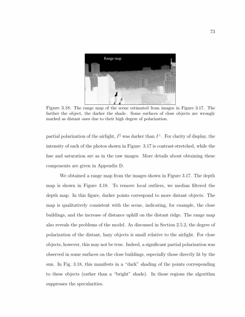
73

Range map

Figure 3.18: The range map of the scene estimated from images in Figure 3.17. Thefarther the object, the darker the shade. Some surfaces of close objects are wronglymarked as distant ones due to their high degree of polarization.

partial polarization of the airlight, I‖ was darker than I⊥. For clarity of display, the

intensity of each of the photos shown in Figure 3.17 is contrast-stretched, while the

hue and saturation are as in the raw images. More details about obtaining these

components are given in Appendix D.

We obtained a range map from the images shown in Figure 3.17. The depth

map is shown in Figure 3.18. To remove local outliers, we median filtered the

depth map. In this figure, darker points correspond to more distant objects. The

map is qualitatively consistent with the scene, indicating, for example, the close

buildings, and the increase of distance uphill on the distant ridge. The range map

also reveals the problems of the model. As discussed in Section 2.5.2, the degree of

polarization of the distant, hazy objects is small relative to the airlight. For close

objects, however, this may not be true. Indeed, a significant partial polarization was

observed in some surfaces on the close buildings, especially those directly lit by the

sun. In Fig. 3.18, this manifests in a “dark” shading of the points corresponding

to these objects (rather than a “bright” shade). In those regions the algorithm

suppresses the specularities.

74

3.8 Summary and Comparison

In this chapter, we presented several algorithms to compute depth information from

one or more images taken in poor visibility conditions. Even though bad weather

is a hindrance to a vision system, it can be put to good use. We showed that

all the single scattering models - attenuation, airlight, contrast (or monochrome),

dichromatic polarization models can be used in various weather and illumination

conditions to compute scaled depth. In all cases, we assumed that the atmosphere

is more or less homogeneous within the field of view.

The attenuation and airlight models were used to compute depth information

separately in special situations of illumination and weather conditions (Sections 3.1,

and 3.2 respectively). Then, several algorithms that took into account the com-

bined effects of attenuation and airlight, were developed. Most of these algorithms

(Sections 3.3,3.4, and 3.6) required multiple images taken under different visibility

conditions. The illumination distribution was assumed to be constant (for example,

overcast sky) between image acquisitions although the global illumination intensi-

ties varied. However, we made no assumption on or used no knowledge of the exact

nature of scene reflectances or the sky apertures of the scene points. On the other

hand, the polarization based algorithm of Section 3.7, did not require weather con-

ditions to change and can be used to compute depth maps of scenes instantaneously.

However, the scene radiances are assumed to be non-polarized. See Figure 3.19 for

a quick comparison of all algorithms presented in this chapter.

How do such scene recovery methods compare with existing ones in com-

puter vision? Unlike binocular stereo, they do not suffer from the problems of

correspondence and discontinuities. Nor do they require tracking of image features

75

ModelAlgorithm ComputedInformation

Input Images Scene

Light Sources

No Restriction

No Restriction

No Restriction

No Restriction

No Restriction

Unpolarized



Section 3.1

Section 3.2

Section 3.3

Section 3.4

Section 3.5

Section 3.6

Section 3.7

Depth Edges

Complete3D Structure

Relative depthsof light sources





Two images ofsources in differentweather at night

Two images indifferent weather



One image indense weather

Two images, onein clear and otherin bad weather

Two images throughdifferent polarizer

orientations.

Dichromatic

Dichromatic

Attenuation

Airlight

Polarization

Figure 3.19: A qualitative comparison of the algorithms for computing depth informationfrom poor weather images.

as in structure from motion. Furthermore, they are particularly useful for scenes

with distant objects (even miles away) which pose problems for stereo and motion.

In the next chapter, we will focus on using the structure information to remove

weather effects from images and video.

76

Chapter 4

Removing Weather Effects from

Images and Videos

Bad weather can severely impact the performance of vision systems. Ultimately, any

vision system must overcome weather effects in order to perform more robustly in

bad weather. Mechanisms can be explicitly or implicitly included in a vision system

to make it robust to weather. In the explicit approach, we may first remove weather

effects from input images/videos using physics-based algorithms to obtain clear day

images. Further tasks (say, tracking, identification, etc) may be then performed

using the deweathered images. In other words, explicit methods preprocess the

images before the images are further analyzed by a vision system. Such methods

allow us to use existing vision systems unchanged. This approach is also useful

when the goal is only to remove weather effects to obtain “good-looking” clear day

pictures for humans to view.

On the other hand, implicit methods simultaneously use physics-based mod-

els and constraints for image understanding in bad weather, as well as the task that

77

a particular vision system does normally. This approach can be task dependent and

hence can be more involved when compared to the explicit approach. However, it

can provide significant flexibility in designing robust measures to overcome weather

effects and at the same time perform the required task. Furthermore, in real-time

tasks, where applying an explicit method is computationally expensive, faster im-

plicit methods may be necessary. Design of implicit methods for a variety of vision

tasks (say, tracking, identification, etc) is set aside for future work.

It is clear that the weather effects depend on the depths of scene points from

the observer. Hence, restoring clear day scene colors and contrasts (deweathering)

from a single image of the scene, without knowing scene structure, is inherently

under-constrained. In this chapter, we will describe a variety of algorithms for

restoring contrasts and colors of the scene irrespective of scene reflectances and

scene structure.

If the scene is at constant depth from the observer (d is same for all pix-

els), weather effects are constant in the entire scene. In this case, simple image

processing algorithms (for example, contrast stretching) can be used to remove the

weather effects. However, for scenes with significant depth variations, traditional

space-invariant image processing techniques will not suffice. We develop three algo-

rithms that are based on the contrast, dichromatic and polarization models. These

algorithms use scene structure computed from poor weather images (as demon-

strated in the previous chapter) to deweather images and videos captured in poor

weather conditions. The algorithms are fast and are linear in image size.

In several situations, structure cannot be computed since multiple images

(captured under different weather conditions or polarizer orientations) may not

78

be available. In such cases, we propose deweathering a single image using simple

additional information provided interactively by the user. Our interactive method

for deweathering can serve as an easy-to-use plug-in for a variety of image processing

software.

In all of our experiments, the images are linearized using the radiometric

response curve of the imaging system that is computed off-line using a color chart.

In addition, multiple images of the scene are acquired with different exposures (or

shutter speeds) and are combined to obtain a high dynamic range maps of the

image irradiances [78].

4.1 Clear Day Contrast Restoration

In this section, we present a method to restore contrast of an arbitrary scene using

scaled depths (3.18) of scene points. We assume that there exists a patch Ezero

in the scene whose direct transmission is zero. This can happen in two instances.

First, Ezero can be a black patch with its scene radiance equal to zero. Note that

the black scene patch will not appear black in the image due to the addition of

airlight. Second, Ezero could be a distant scene patch that is completely invisible

due to strong airlight. In other words, this distant scene patch has zero direct

transmission and its contrast cannot be restored from a bad weather image.

We can either mark such a patch manually or detect one automatically from

the image. An algorithm to detect zero direct transmission patches automatically

in weather degraded images is presented in the next section. Since the apparent

brightness of the patch Ezero is solely due to airlight, its optical depth can be

computed as,

β dzero = − ln (1 − Ezero/I∞) . (4.1)

79

Then, the optical depth of any other scene point Pi is obtained using,

β di = (β dzero)

(di

dzero

), (4.2)

where, the second term can be computed using the ratio of scaled depths (see

(3.18)). Then, the normalized radiance ρi of the scene point Pi is estimated using

(2.19). Recall that ρ does not depend on the weather condition (β, I∞). Thus, by

computing ρ for each scene point, we restore contrast of the entire scene.

Note that structure computation requires two images to be taken under

different weather conditions but under similar daylight spectra. However, once

scene structure is computed, contrast can be restored from a single image of the

scene taken under arbitrary weather and illumination conditions.

Experimental Results

Results of experiments performed on images of a real scene are shown in Figures 4.1.

Figures 4.1(a,b) show two high dynamic range images of the same scene captured

under different conditions of mist (light and moderate). The depth map computed

is shown in Figure 4.1(c). Notice the windows of the farther buildings that are

clearly visible in (d) as compared to the images in (a). In general, removing the

spatio-temporal effects of rain is a much harder problem compared to more stable

weather conditions such as fog, mist, and haze. The brightnesses due to rain drops

in the scene cannot be modeled using the simple direct transmission and airlight

models used in this thesis. However, for faraway scenes with no significant spatio-

temporal effects, we could apply our technique for rain images as well.

Experiments with Video : Moving Objects

Consider an outdoor surveillance video camera capturing a scene (with moving

objects) over an extended period of time. We would like to process this video in

80

(a), (b) Images taken at 3pm and 4pm under poor visibility conditions (mist)

(c) Computed depth map (d) Contrast restored Image (from (b) and (c))

(f) Computed contrast restored image (from (e) and (c))(e) Image taken in rainy conditions

Figure 4.1: [a - d] Structure computation and restoration of image contrast from twoimages taken under poor visibility conditions. The depth map is median filtered andaveraged to reduce noise. Notice the significant increase in contrast in the farther build-ings. Contrast stretching is applied to all the images for display purposes. [e-f ] Contrastrestoration from one bad weather (in this case, rain) image and pre-computed scenestructure. The depth map computed from two misty images (in (c)) was used to restorecontrast from just one image of the same scene under rain. The rainy image shown in (e)and the misty images shown in (a) and (b) were captured on different days. (f) Contrastrestoration using the algorithm proposed.

81

real-time to obtain a weather-free video. Note that our algorithms cannot remove

temporal effects of rain from a video of a rainy scene. For the purposes of discussion,

we define the static part of the scene as the background, and the moving objects

in the scene as the foreground. The foreground objects can be separated from the

background using any background subtraction method (for instance, [127]). Then,

weather-free video is obtained using an algorithm that has the following two stages:

• Initialization stage : We first detect any change in weather condition us-

ing normalized SSD (section 3.3). Then, the two frames that correspond to

the different weather conditions are used to compute scaled depths of the

background scene (section 3.4).

• Contrast Restoration : Note that the methods we described hitherto can-

not be used to restore contrast of moving objects since their depths are un-

known. Therefore, heuristics are needed to assign depths to foreground ob-

jects. One conservative heuristic is to examine the depths in a neighborhood

around each moving object and assign the minimum depth to it. The algo-

rithm presented in section 4.1 can then applied to the entire frame to restore

scene contrast.

Experimental results with a video of a traffic scene taken under foggy condi-

tions are shown in Figure 4.2. We used an off-the-shelf 8-bit digital video camera

and captured two short video clips half an hour apart. As described in previous

experiments, we linearized the frames with the radiometric response function of the

video camera. We averaged 100 frames in each video clip to reduce noise and used

the resulting images to compute structure of the background scene (buildings). The

82

1 2

4

3

(a) Scene imaged at 5 : 00pm. (b) Scene imaged at 5 : 30pm

(c) Depth map computed from (a) and (b) (d) Contrast restored using (b)

Figure 4.2: Experiments with videos of a traffic scene on a foggy day. (a)−(b) Two shortvideo clips were captured half an hour apart using an 8-bit video camera. 100 frameswere averaged to reduce noise. Note that the vehicles on the road in the two images aredifferent. (c) The depth map was computed for the background image using the algorithmpresented in section 5. The scaled depths of the region corresponding to the road werelinearly interpolated using scaled depth values at pixels on the left and right corners ofthe road. (d) The de-fogged (contrast restored) image obtained from the frame in (b).Compare the contrast restored image with the histogram equalized image in Figure 4.4.

83

After

Before 1 2 3 4

Figure 4.3: Zoomed in regions of the frame (see the marked rectangles in Figure 4.2(b))demonstrate the significant increase in contrast at various depths of the scene. Note thatdifferent amounts of fog were removed at different depths. Also, notice the better contrastof moving objects (vehicles).

Figure 4.4: Artificial contrast enhancement (not contrast restoration) of a foggy imageby histogram equalization does not remove fog completely at all depths in the scene. Inthis example, farther depths have poorer contrast when compared to the nearer depths.

scaled depths in the road region were linearly interpolated using scaled depth values

at pixels on the left and right corners of the road. Then, contrasts of buildings,

the road and moving vehicles were restored for each frame of the video. Notice the

significant increase in contrast at various depths in the scene (Figures 4.2(d) and

4.3). In our current implementation, contrast restoration was applied to the video

off-line.

84

4.2 Clear Day Scene Colors using Dichromatic Model

In this section, we compute the scene colors as they would appear on a clear (but

overcast day) from two bad weather images. More precisely, we compute the direct

transmission colors of the entire scene using minimal a priori scene information.

For this, we first show that, given additional scene information (airlight or direct

transmission vector) at a single point in the scene, we can compute the clear day

colors of the entire scene from two bad weather images.

Consider the dichromatic model given in (2.27). The color of a scene point

Pi under weather condition β is,

E(i) = p(i) D(i) + q(i) A , (4.3)

where p(i) is the direct transmission magnitude, and q(i) is the airlight magnitude

of Pi. Suppose that the direction D(i) of direct transmission color for a single point

Pi is given. Besides, the direction A of airlight color for the entire scene can be

estimated using (3.21). Therefore, the coefficients p(i) and q(i) can be computed

using (4.3). Furthermore, the optical thickness βdi of Pi can be computed from

(2.28).

Since we have already shown how to compute the scaled depth of every scene

point (see (3.26)), the relative depth dj / di of any other scene point Pj with respect

to Pi can be computed using the ratio of scaled depths. Hence, the optical thickness

and airlight for the scene point Pj, under the same atmospheric condition are given

by,

βdj = βdi (dj / di) ,

q(j) = E∞(1 − e−βdj ) . (4.4)

85

R

GB q

D∧

~q

O

E∧-A

Figure 4.5: The observed color E of a scene point, its airlight direction A and clearday color direction D are shown in the R-G-B color cube. q is the distance from E to asurface of the cube along negative A. For scene points whose clear day colors do not lieon the cube surface, q is greater than the true airlight magnitude q.

Finally, the direct transmission color vector of Pj can be computed as

p(j) D(j) = E(j) − q(j) A . (4.5)

Thus, given a single measurement (in this case, the direction of direct transmission

color of a single scene point), we have shown that the direct transmission and airlight

color vectors of any other point, and hence the entire scene can be computed. But

how do we specify the clear day color of any scene point without actually capturing

the clear day image?

For this, we assume that there exists at least one scene point whose direct

transmission color D lies on the surface of the color cube (including origin or black)

and we wish to identify such point(s) in the scene automatically. Consider the R-

G-B color cube in Figure 4.5. If the clear day color of a scene point lies on the

surface of the color cube, then the computed q is equal to the airlight magnitude q

of that point. However, if it lies within the color cube, then clearly q > q.

86

(b) Output: Dehazed 3D views

(a) Input : Images taken with Mild and Dense haze

Figure 4.6: Effective structure computation and color restoration in haze. The inputimages acquired under different hazy conditions are used to compute the scene structureby applying the dichromatic color constraints based algorithm in Section 3.6. Then, thealgorithm proposed in this section is used to deweather the images. The rotated three-dimensional illustrations are texture mapped with the dehazed result. The depth mapwas smoothed using median filtering. Two more views of the depth map are shown inFigure 4.7.

87

Figure 4.7: Two additional views of the rotated depth maps obtained from the inputhazy images in Figure 4.6.

For each point Pi, we compute q(i) and optical thickness β1di. Note that

β1di may or may not be the correct optical thickness. We normalize the optical

thicknesses of the scene points by their scaled depths (DOTs) to get

αi =β1di

(β2 − β1)di. (4.6)

For scene points that do not lie on the color cube surface, αi is greater than what

it should be. Since we have assumed that there exists at least one scene point

whose clear day color is on the surface of the cube, it must be the point that has

the minimum αi. So, q(i) of that point is its true airlight. Hence, from (4.4), the

airlights and direct transmission colors of the entire scene can be computed without

using a clear day image. For robustness, we use k least αi′s. We call this the Color

Cube Boundary Algorithm.

Figure 4.6 illustrates experiments with a real scene. Usually in urban scenes,

window interiors have very little color of their own. Their intensities are solely

due to airlight and not due to direct transmission. In other words, their direct

88

transmission color is black (the origin of the color cube). We detected such points

in the scene using the above technique and recovered the clear day colors of the

hazy scene.

4.3 Instant Dehazing using Polarization

In this section, we present a simple algorithm to remove effects of haze using po-

larization filtering. Two images, I‖ and I⊥, are acquired by varying the polarizer

orientation. From equations 2.35 and 2.38, the airlight can be computed from the

polarization components, I‖ and I⊥ as:

A =I⊥ − I‖

P, (4.7)

Then, the direct transmission is computed as

D = Itotal − A = I‖ + I⊥ − A . (4.8)

In this image the additive effect of the airlight is removed. Recall that beside

the addition of airlight, the haze attenuates the light coming from the object. By

compensating for the attenuation of the transmitted light, we obtain an estimate

for the scene radiance that would have been measured in the absence of atmospheric

scattering:

R =Itotal − A

e−βd=

Itotal − A

1 − A/E∞. (4.9)

R is hence the dehazed image. We measure the values for E∞ and P from the sky

as described in Section 3.7. For mild haze under sunny skies, note that E∞, P and

β are functions of the light wavelength λ. For this reason the airlight in moderate

haze is typically bluish. In order to account for the wavelength dependence, it is

best to analyze the images with high spectral resolution. Since we only have RGB

channels in our camera, we performed the analysis for each channel independently.

89

(c) Computed Depthmap (d) Computed De-hazed Image

(b) Input : Maximum polarization(a) Input : Minimum polarization

Figure 4.8: Instant dehazing of images using polarization. Two images acquired byvarying the polarizer orientation are used to compute the range map as well as a dehazedview of the scene. Notice the significant improvement in contrast and color in the dehazedimage.

We applied this algorithm to the images shown in Figures 4.9 and 4.8. The dehazed

image has much better contrast and color than what optical filtering alone yields,

especially in the distant regions of the scenes. Moreover, the algorithm removed the

blue color bias, which existed in the raw images. Thus the green forest is clearly

visible in the distant scene, while in the raw images that area looks like grayish-blue

noise (Figure 4.9). The colors of the red bricks and roofs of the distant buildings

are also restored. The improvement of color is also seen in the closer objects, like

the orange building on the right, where the blue airlight was weaker.

90

Before

After

(d) Zoomed in regions showing color restoration

(c) Computed De-hazed Image

(b) Input : Maximum polarization(a) Input : Minimum polarization

Figure 4.9: Instant dehazing of images using polarization. Two images acquired byvarying the polarizer orientation are used to compute a dehazed view of the scene. Noticethe significant improvement in contrast and color in the output image. In the magnifiedimage portions, note the green forest and lawns, the red roofs of the houses and the whitebuildings on the ridge.

91

4.4 Interactive Deweathering

In this section, we address the question of how to deweather a single image of a

scene without using precise depth information. In the previous sections, we showed

that multiple images of the same scene are necessary to compute scene structure

which can then be used for deweathering. However, in many cases, it may not

be possible to acquire multiple images. For instance, today there are millions of

pictures corrupted by weather, that are taken by amateur and professional photog-

raphers, with virtually no information about the depths or the atmosphere tagged

to them. Very often, all we may have is a single photograph of a scene that we

wish to deweather. In such cases, we will show that using minimal additional input

from the user can successfully break the ambiguities in deweathering an image.

Based on the contrast and color models, we present two algorithms to in-

teractively deweather a single image. In both these cases, the user provides sim-

ple inputs through a visual interface to our physics-based algorithms for restoring

contrasts and colors of the scene. The types of input (for instance, approximate

direction in which scene depths increase, or a rough depth segmentation or a region

of good color fidelity) may vary from scene to scene, but are easy to provide for a

human user. We show several results that illustrate effective deweathering of both

color and gray-scale images captured under harsh weather conditions. Since the

algorithms do not require precise information about scene structure or atmospheric

condition, they serve as easy-to-use plug-ins for existing image processing software,

such as Adobe PhotoshopTM . We believe that our interactive methods will make

deweathering widely applicable.

92

4.4.1 Dichromatic Color Transfer

Consider a scene with points at different depths but with similar clear day colors.

For instance, trees at different distances, or buildings at different depths, may have

similar color directions (although their magnitudes may vary) on a clear day. In

this scenario, the colors of near scene points are less corrupted by bad weather as

compared to the distant scene points. We now describe an algorithm to transfer

colors from nearby regions to replace colors of regions that are most effected by bad

weather, in a physically consistent manner. In other words, we impose constraints

based on the dichromatic model (2.27,2.28) to select colors of near scene points to

replace colors of far scene points.

Interactive Step: Only two manual inputs are necessary for the color transfer

algorithm. First, we select a nearby “good” region in the image, where colors D

are not corrupted (or, minimally altered) by bad weather, as shown by the white

rectangle in Figure 4.10(a). Then, we mark a region (say, sky) that most resembles

the color of airlight, as shown by the black rectangle in Figure 4.10(a)1. The average

color within this region is computed to estimate the direction A of airlight color.

Automated Step: For each pixel, with color Ei, in the weather effected region,

we search for the best matching color in the “good” region. The search is restricted

to a set of pixels in the “good” region that satisfy the dichromatic planarity (2.27),

Ei.(D × A) = 0 .

From this set, we choose a pixel whose color Di is farthest (in terms of angle) from

1If such a region does not exist in the image, then the user may provide the hue of the sky andassume the sky intensity to be the maximum intensity in the image. Another way of computingthe color of airlight is by intersecting dichromatic planes of two different user provided scene colors(Section 3.6).

93

(a) Input : Misty image (b) Output : Color corrected image

User selectedGood color region

User selectedAirlight color

Figure 4.10: Color correction by dichromatic color transfer. (a) Input misty imageconsisting of green bushes at different distances. A region of “good” color is marked inthe white rectangle. A region that most resembles the color of mist is marked in theblack rectangle. (b) Colors from the near “good” region are transfered to farther regions.Notice the bluish colors of the farther bushes replaced by greenish colors.

the fog color A, using

min D.A .

In order to compute the magnitude of the color used to replace the pixel Ei, we use

the dichromatic model (2.27) to decompose the scene color Ei into two components

:

Ei = p Di + q A .

Finally, we replace the color Ei of the pixel by the deweathered color, p Di. Note

that the ambiguities in the dichromatic model are broken due to the presence of

similar colored scene points at different distances. This algorithm does not require

any information regarding scene depths or atmospheric conditions. Further, it does

not assume homogeneity of the atmosphere over the entire field of view. The result

of applying this method is shown in Figure 4.10 (b). Notice the significant change

in the colors of the far bushes.

94

4.4.2 Deweathering using Depth Heuristics

A limitation of the color transfer method is that all colors in the weather effected

region may not have corresponding colors in the “good” color region. In this sec-

tion, we describe deweathering using heuristics on scene depths. Note that subtle

weather effects within small depth ranges are not captured by a camera with lim-

ited dynamic range (say, 8 bits). Therefore, precise distances are not required for

effective deweathering. Moreover, in many cases, it may be possible to input ap-

proximate “trends” in the depths of scene points (say, the direction of increasing

depths). For instance, a scene with a street along the viewing direction is common

in surveillance or tracking scenarios (see Figure 4.14). The deweathering algorithm

is detailed below.

Interactive Step: We select a region of the sky to obtain the sky intensity E∞

(and sky color direction A, if the input is a color image). Then, the “depth trend”

is interactively specified in the following manner. First, we input the approximate

location of a vanishing point along the direction of increasing distance in the image

(see red circle in Figure 4.12). The distances of the scene points are inversely related

to their image distances to the vanishing point. Next, we input the approximate

minimum and maximum distances and interpolate distances (say, using a linear or

quadratic function) for points in between. For illustration purposes, we used

d = dmin + α (dmax − dmin) , (4.10)

where, α ∈ (0, 1) is the fractional image distance from a pixel to the vanishing

point. For d = dmax , α = 1 and for d = dmin , α = 0 . The resulting depth trend is

shown in Figure 4.11 (a).

Automated Step: The contrast or monochrome model (Section 2.3) for the

95

0.5

1

1.5

2

2.5

Sky region

0.5

1

1.5

2

2.5

3Sky region

0.5

1

1.5

2

2.5

3Sky region

(a) (b) (c)

Figure 4.11: Depth heuristics used to deweather images shown in Figures 4.12, 4.13and 4.14 respectively. The vanishing point corresponding to the direction of increasingdistances is marked. Approximate minimum and maximum distances are input to thealgorithm and the intermediate distances are interpolated. The depths are not used forsky regions (empty spaces).

intensity E of a scene point in bad weather, recorded by a monochrome camera,

can be rewritten as:

E = Re−βd + E∞(1 − e−βd) , (4.11)

where R is radiance of the scene point on a clear day. At every pixel, the depth

estimate d is known, and the sky brightness E∞ is measured. Generally, the at-

mosphere condition remains constant (or varies slowly) over small distance ranges

and fields of view that are relevant to computer vision applications. If we assume

homogeneity of the atmosphere, then the scattering coefficient β is constant for all

pixels in the image. Then, note that different values of the scattering coefficient

β produce the effects of different densities of bad weather (moderate, heavy, etc.).

Thus, by continuously changing β (imagine a slider in Adobe PhotoshopTM), we

can progressively estimate the clear day radiances R at each pixel as,

R = [E − E∞(1 − e−βd)] eβd . (4.12)

Similarly, note that the dichromatic model (equation 2.27) can be used to restore

colors in an RGB image. Therefore, while the color transfer method can be applied

96

(a) Input : Misty image

(c) Zoomed-in regions of (a)

(b) Output : Deweathering to different extents(by choosing different values for )

(d) Contrast and color restoration in zoomed-in regions.

User selectedVanishing Point

User selectedSky Brightness

Figure 4.12: Restoring clear day scene colors using depth heuristics. (a) Input imagecaptured in mist. The colors and contrasts of scene points, especially in farther regions,are corrupted severely. (b) Two images illustrating different amounts of mist removedfrom the image in (a). These images were computed using the depth “trend” shownin Figure 4.11(a). (c) Zoomed in regions selected from (a) at different depths showingdifferent amounts of mist. (d) Corresponding zoomed in regions of the deweatheredimages. Notice the significant contrast enhancement.

only to color images, this method can be applied to both color and gray-scale

images. In this case, the homogeneity of the atmosphere breaks the ambiguity in

deweathering an image. The results shown in Figures 4.12, 4.13 and 4.14 illustrate

that approximate depth information can be used effectively for image deweathering.

97

(a) Input : Misty image



(d) Contrast and color restoration in zoomed-in regions.



Figure 4.13: Restoring clear day scene colors using depth heuristics. (a) Input imagecaptured in mist. The colors and contrasts of scene points, especially in farther regions,are corrupted severely. (b) Two images illustrating different amounts of mist removedfrom the image in (a). These images were computed using the depth “trend” shownin Figure 4.11(b). (c) Zoomed in regions selected from (a) at different depths showingdifferent amounts of mist. (d) Corresponding zoomed in regions of the deweatheredimages. Notice the significant quality improvement.

98

(a) Input : Foggy image



(d) Contrast restoration in zoomed-in regions.



Figure 4.14: Restoring clear day scene contrasts using depth heuristics. (a) Input gray-scale image captured in fog. The contrasts of scene points, especially in farther regions,are degraded severely. (b) Two images illustrating different amounts of fog removed fromthe image in (a). These images were computed using the depth “trend” shown in Figure4.11(c). (c) Zoomed in regions selected from (a) at different depths showing differentamounts of fog. (d) Corresponding zoomed in regions of the deweathered images. Noticethe significant contrast enhancement.

99

4.5 Summary

Images captured in bad weather have poor contrasts and colors. These weather

effects must be removed in order to reliably perform further vision-based analysis

on the images. However, since weather effects depend on the depths of scene points,

simple image processing will not suffice. In this chapter, we presented a set of

algorithms to restore clear day contrasts and colors of scene points using scene

structure computed using the algorithms described in Chapter 3. We demonstrated

the effectiveness of the algorithms using experiments on several scenes captured

in poor weather conditions. Finally, we presented a set of interactive tools to

approximately deweather images when precise relative depth information is not

available.

Chapters 3 and 4 illustrated the usefulness of single scattering models for

scene interpretation. In the next part of the thesis, we present a multiple scattering

model and present applications in scenarios where multiple scattering is significant

and cannot be neglected.

Part III

Multiple Scattering in

Participating Media

100

102

Chapter 5

A Multiple Scattering Model and

its Applications

Virtually all methods in image processing and computer vision, for removing weather

effects from images, assume single scattering of light by particles in the atmosphere.

It is assumed that the irradiance at any pixel is solely due to scattering within a

small column of the atmosphere along the pixel’s line of sight. The previous parts

of this thesis demonstrated the validity of this assumption in a variety of weather

conditions, using several experiments. In these cases, single scattering dominates

multiple scattering in the measured image irradiance. However, there are situations

when multiple scattering can be significant and cannot be therefore neglected. A

common manifestation of multiple scattering is the appearance of glows around

light sources in bad weather. Figure 5.1 shows glows around light sources on a

misty night. Light from the sources gets scattered multiple times and reaches the

observer from different directions (Figure 5.2). Modeling multiple scattering is crit-

ical to completely understand the complex effects of weather on images, and hence

103

Figure 5.1: Night image of light sources in mist. The glows around sources reveal theweather condition, as well as the relative depths and shapes of sources.

Light Source

Glow in Image Plane

Pinhole

AtmosphereMultiple Scattered Light

Unscattered Light

Figure 5.2: Multiple scattering of light from a source to a sensor results in an imagewith a glow around the source.

essential for improving the performance of outdoor vision systems.

The complexity of modeling the traversal of light rays through the atmo-

sphere is well known. One approach to solve this problem is to assume the paths of

light traversal to be random and then to apply numerical Monte-Carlo techniques

for ray tracing [6]. Computer graphics researchers [82; 112] have followed this ap-

proach (as well as approximations [50] like diffusion and single scattering) to render

scenes in scattering media. However, millions of rays must be traced through the

atmosphere to accurately model multiple scattering. Clearly, the computational

complexity of this approach is too high to be suitable for most vision (or even

graphics) applications.

In this chapter, we develop a new physics-based and analytic model for the

multiple scattering of light rays as they travel from a light source to an observer.

104

This model is derived using the theory of light or radiative transport. The model

is valid for various weather conditions including fog, haze, mist and rain. We

demonstrate two applications that are relevant to the fields of Computer Graphics

and Computer Vision. From the perspective of Computer Graphics, we demonstrate

rendering of multiple scattering effects that is orders of magnitude faster than

the existing Monte Carlo approaches. This is referred to as the forward problem.

From the perspective of Computer Vision, the inverse problem is more interesting.

Our model enables us to recover from a single image the shapes and depths of

sources in the scene. In addition, the weather condition and the visibility of the

atmosphere can be estimated. These quantities can, in turn, be used to remove

the glows of sources to obtain a clear picture of the scene. Based on these results,

we demonstrate that a camera observing a distant source can serve as a “visual

weather meter”. Although we have concentrated mostly on scattering within the

atmosphere, our model is applicable to other scattering media such as fluids and

tissues.

We begin by giving a brief description on the theory of Radiative Transfer.

Then, we present a detailed derivation of the model for multiple scattering. The

model is extensively validated and two applications of this model are presented.

5.1 Introduction to Radiative Transfer

The study of propagation of radiation through particulate media is commonly re-

ferred to as Radiative Transfer [17; 48]. Radiative transfer has been a major area of

research in several fields including atmospheric optics, thermodynamics, astronomy,

nuclear physics, oceanography, medical imaging and remote sensing. Although the

applications of interest vary greatly among these areas, the theory of radiative trans-

105

Light Incidentfrom all Directions

Exiting Light Radiance

Infinitesimal Element of the Atmosphere

Figure 5.3: An infinitesimal volume of a medium illuminated from all directions. Theradiative transfer equation (RTE) describes the relationship between scattered light ra-diance (in a particular direction) and the irradiance incident (from all directions) for theinfinitesimal volume.

fer provides a common mathematical framework for analyzing problems related to

propagation of radiation that arise in these applications.

The basic idea in radiative transfer is to investigate the difference between

light incident on, and exiting from, an infinitesimal volume of the medium, as shown

in Figure 5.3. Mathematically, the change in flux through a small volume is given

by an integro-differential equation, called the Radiative Transfer Equation (RTE).

The directional intensity at any location (light field) in the medium is then obtained

by solving this equation. The forward problem in radiative transfer is defined as

the computation of the scattered light field in the medium given the properties of

the medium and the sources. Similarly, the inverse problem can then be defined

as the estimation of the properties of the medium and sources, given the scattered

light field. The exact form of the RTE depends on the locations and types of the

radiation sources and the types and distributions of particles within the medium.

Although their exact mathematical forms can be complex, the RTEs present a clean

framework for describing multiple scattering within media.

106

T = 0

T

Incident Illumination

Homogenous Medium

I (T, µ)

Figure 5.4: Plane parallel model used by most previous works to describe multiplescattering and diffusion. The source is generally collimated and is outside (infinitely faraway from) the medium. Such a model can be used for scattering in clouds, for instance,but not for cases where the source is divergent and is within the scattering medium.

5.1.1 Forward Problem

Research focusing on solving the forward problem in radiative transfer has been

pursued for the past several decades. At a high level, we can classify the literature

in radiative transfer into the three categories - (a) methods that use computationally

intensive numerical techniques to simulate transfer through media [6], (b) analytic

approximations to radiative transfer such as diffusion [48] and single scattering [12;

4; 61] and (c) analytic solutions to specific radiative transfer equations [17].

While it is desirable to obtain analytic solutions to the transfer equation, it is

generally hard. Several works [123; 17] on deriving analytic solutions have focused

on the plane parallel RTE (see Figure 5.4) and its variations, where usually the

radiation source is outside the medium. For instance, this has been an important

RTE for researchers in atmospheric optics and astronomy where the medium (say,

atmosphere around the earth or a star) is illuminated by a distant source (say, sun

or the deep core of the star).

For applications where the sources are within media, the plane parallel ge-

ometry is not necessarily the most intuitive geometry for the scattering medium.

Consider for example the glow around an outdoor lamp in fog. In this case, it is

107

better to approximate the medium surrounding the lamp by a sphere rather than

a plane parallel medium and hence light transport should be analyzed using the

spherical RTE rather than the plane parallel RTE. Similarly, other scenarios where

light sources are within media are seen in medical imaging (endoscopy) or under-

water imaging. As compared to the plane parallel RTE, very little work has been

done on the analytic solution of a spherical RTE. Exceptions have been the works

where the RTE has been solved either (a) by assuming isotropic scattering [17;

69], or (b) by solving for the average (total) intensity at any spatial location in the

medium [5; 28], instead of the directional intensities required to solve the forward

problem.

In this chapter, we present an analytic series solution to the radiative transfer

from an isotropic source present in a homogeneous spherical medium (described by

the spherical RTE). This solution accounts for both isotropic and anisotropic phase

functions as well as absorbing and purely scattering media. The series solution

is compact and can be used to compute the scattered light field almost instanta-

neously.

5.1.2 Inverse Problem

While there has been considerable success in solving the forward RTE, the in-

verse RTE is generally ill-posed [6]. However, in special cases, several studies

have attempted to solve the inverse RTE. It has been shown that light sources

as seen through a medium (say, atmosphere), provide cues about the medium

as well as the sources themselves. For instance, in astronomy, telescopic images

of stars have been used to extract the shapes of the stars as well as informa-

tion about the atmospheres surrounding the stars [16]. In atmospheric optics,

108

the fuzzy appearance of the sun (or moon) behind a cloud [67] has been used

to recover scattering properties of particles in the cloud [6; 60]. The aureole

seen around the moon during a solar eclipse provides information about the sun’s

corona and atmospheric aerosols [30]. The above works take into account multi-

ple light scattering but the plane parallel RTE used in these cases (plane parallel

model for radiative transfer shown in Figure 5.4) is not applicable to our setting

where the source is inside a scattering medium. Exceptions are the works of [96;

14] which use the single scattering approximation to respectively estimate optical

thickness and the properties of rainfall from observed peaks in multiple scattered

intensities. In this work, for the case of purely scattering media, we will show that

a simple two-parameter non-linear optimization can be used to solve the inverse

RTE.

We begin by describing the spherical RTE and then derive an analytic solu-

tion to the forward problem. Then, we validate the solution using extensive simula-

tions as well as real experiments in two media - atmosphere and milk. Although the

work focuses on the atmosphere and milk, the results can be used analyze radia-

tive transfer from sources through virtually any particulate medium such as smoke,

tissue and blood. The most prominent resources for our work will be the classical

textbooks of Chandrasekhar [17], Ishimaru [48], and Sobolev [123] on the theory of

radiative transport.

109

IsotropicPoint Source

0I

Homogeneous Medium

RadiusR

θI (T, )µ

Light Field

Figure 5.5: Illustration of an isotropic point source illuminating a homogeneous sphericalscattering medium. The multiple scattered light field in the medium depends on radialoptical distance T = σR and the direction θ from the radial direction.

5.2 Spherical Radiative Transfer

In this section, we describe the type of medium and the source and hence write the

equation of transfer for this setting.

5.2.1 Medium and Source Geometry

Consider a homogeneous scattering medium as shown in Figure 5.5. The isotropic

point source at the center illuminates the medium. The light field due to this

source is said to exhibit spherical symmetry. In other words, the light field I in the

medium only depends on the radial optical distance T = σR (σ is the extinction

coefficient) and angle θ = cos−1 µ from the radial direction and is expressed in

terms of a Legendre polynomial series. We call the multiple scattered light field as

just the point spread function (PSF).

5.2.2 Phase Function of Medium

When light is incident on a particle, it gets scattered in different directions. This

directional distribution of light is called the phase function of the particle. The

phase function is denoted by P (θ, φ; θ′, φ′) and it specifies the scattered radiance

110

P( cos α )

Scatterer

Incident Light α( , )θ’ φ’

( , )θ φ

(a)

q0.0 1.00.2 0.4 0.7 0.8

Air Haze Fog RainMist Small Aerosols

0.9

(b)Figure 5.6: (a) The phase function P (cos α) is the angular scattering distribution ofa particle. For most atmospheric conditions, P is symmetric about the incident lightdirection. The exact shape of P depends on the size of the scatterer, and hence theweather condition. Often the phase function can be written using a Legendre polynomialseries. (b) The approximate forward scattering parameter q of the Henyey-Greensteinphase function for various weather conditions. Note that the boundaries between theweather conditions are not clearly defined.

in the direction (θ, φ) for the incident irradiance from (θ′, φ′). For most media, the

phase function is known to be symmetric about the direction of incident light [17].

So, P depends only on the angle α between the directions of incident and scattered

radiation (Figure 5.6), which is determined as:

cos α = µµ′ +√

(1 − µ2)(1 − µ′2) cos(φ − φ′) , (5.1)

where, µ = cos θ and µ′ = cos θ′.

The exact shape of the phase function depends on the size of the scattering

particle, and hence the type of weather condition [47]. For instance, phase functions

of small particles (say, air molecules) have a small peak in the direction of incidence.

Isotropic [P (cosα) = constant] and Rayleigh [P (cosα) = 3/4(1 + cos2 α)] phase

functions describe the scattering from air molecules. On the other hand, phase

functions of large particles (say, water droplets in fog) have a strong peak in the

111

direction of light incidence. A more general phase function that holds for particles

of various sizes is the Henyey-Greenstein phase function [44]:

P (cosα) =1 − q2

(1 + q2 − 2q cos α)3/2, (5.2)

where, q ∈ [0, 1] is the called the forward scattering parameter. If q = 0, then the

scattering is isotropic, and if q = 1, then all the light is scattered by the particles in

the forward (incident or α = 0) direction. Values for q between 0 and 1 can generate

phase functions of most weather conditions. In general, the phase function can be

written using a Legendre polynomial series [48]:

P (cosα) =∞∑

k=0

Wk Lk(cos α) . (5.3)

where, Wks represent the shape of the phase function. Equation 5.3 holds for both

isotropic as well as anisotropic phase functions and thus is valid for most scattering

media. For the Henyey-Greenstein phase function (5.2), Wk = (2k + 1) qk [48].

5.2.3 Spherically Symmetric RTE

Given the above descriptions for the medium and source illuminating the medium,

the RTE for a spherically symmetric atmosphere [17] is mathematically written as,

µ∂I

∂T+

1 − µ2

T

∂I

∂µ= −I(T, µ) +

1

4π

2π∫0

+1∫−1

P (µ, φ; µ′φ′) I(T, µ′)dµ′ dφ′ , (5.4)

Here, P (µ, φ; µ′φ′) is the phase function of the particles in the medium. cos α is the

angle between incoming irradiance in the direction (θ′, φ′), and outgoing scattered

radiance in the direction (θ, φ). The angles (θ, θ′) are written in terms of their

cosines as µ = cos θ.

112

5.3 The Forward Problem in Spherical Radiative Transfer

The forward problem in radiative transfer is defined as the computation of the

radiation (light) field in a medium given the scattering properties (say, extinction

cross section and phase function) of the medium. In this section, we present the

derivation of an analytic form for I(T, µ). The derivation is divided into four major

steps and the details of each step are described below.

5.3.1 Eliminating Partial Derivative ∂I∂µ

In the first step, we eliminate the partial derivative of I with respect to µ by

integrating the RTE with respect to µ over the range [−1, +1]. Most of the details

of this step are adapted from [17]. However, a key difference in our approach to

eliminating the partial derivative is to use exact integrals instead of approximating

the integrals by linear summations [17].

By integrating the phase function P over the azimuth angle φ′, Ishimaru [48]

and Chandrasekhar [17] define a function that does not depend on the azimuth

angle as,

P (0)(µ, µ′) =1

2π

2π∫0

P (cosα)dφ′ , (5.5)

where,

cos α = µµ′ +√

(1 − µ2)(1 − µ′2) cos(φ − φ′) , (5.6)

and, µ = cos θ and µ′ = cos θ′. As we shall see, the use of P (0) simplifies the

mathematics involved in modeling the multiple scattering around a point light

source. Substituting into equation 5.4 we get,

µ∂I

∂T+

1 − µ2

T

∂I

∂µ= −I(T, µ) +

1

2

+1∫−1

P (0)(µ, µ′) I(T, µ′)dµ′ . (5.7)

113

Chandrasekhar [17] defines a function Qm(µ), for some m > 0, such that

Lm(µ) = −d((1 − µ2)Qm(µ))

dµ⇐⇒ Qm(µ) =

L′m(µ)

m(m + 1)(5.8)

Consider the integral+1∫

−1

(1 − µ2) Qm

(∂I

∂µ

)dµ . (5.9)

Integrating by parts and using 5.8, it has been shown that we can eliminate the

partial derivative with respect to µ (see [17]),

+1∫−1

(1 − µ2) Qm

(∂I

∂µ

)dµ =

+1∫−1

I(T, µ)Lmdµ . (5.10)

When there is no confusion, we drop the parameters µ and T for brevity. Multi-

plying 5.7 by Qm and integrating with respect to µ over [−1, +1], we get,

+1∫−1

µQm∂I

∂Tdµ +

+1∫−1

1 − µ2

TQm

∂I

∂µdµ =

−+1∫

−1

QmI dµ +1

2

+1∫−1

Qmdµ

+1∫−1

P (0)(µ, µ′) I(T, µ′)dµ′ , (5.11)

Substituting equation 5.10, we can rewrite the RTE as,

+1∫−1

µQm∂I

∂Tdµ +

1

T

+1∫−1

LmI dµ =

−+1∫

−1

QmIdµ +1

2

+1∫−1

Qm(µ)dµ

+1∫−1

P (0)(µ, µ′) I(T, µ′)dµ′ , (5.12)

Thus, the partial derivative with respect to µ is eliminated from the RTE leaving

only the derivative with respect to the optical thickness T .

5.3.2 Legendre Polynomials for I(T, µ) and P (0)

This is the key section in the derivation of our model. We assume that a solution

Im(T, µ) to (5.12) is a product of two functions - g(T ) depending only on the optical

114

thickness T , and f(µ) expressing the angular dependence. This approach has also

been taken for other RTEs in previous work. Mathematically,

Im(T, µ) = gm(T )fm(µ) . (5.13)

Substituting into 5.12, we get,

g′m

+1∫−1

µQmfmdµ +gm

T

+1∫−1

Lmfmdµ + gm

+1∫−1

Qmfmdµ −

gm

2

+1∫−1

Qmdµ

+1∫−1

P (0)(µ, µ′) fm(µ′)dµ′ = 0 . (5.14)

Since the RTE is spherically symmetric (does not depend on the azimuth angle

φ), we know that a Legendre polynomial expansion (and not a spherical harmonic

expansion) of I is possible. Therefore, suppose

fm(µ) = Lm−1 + Lm , (5.15)

for some m > 0. As we shall show, the above form is key to get a non-trivial

solution to the RTE ensuring none of the terms of the RTE go to zero. Since the

phase function P is symmetric about the direction of the incident light, P can be

expanded using Legendre polynomials as

P (cosα) =∞∑

k=0

Wk Lk(cos α) . (5.16)

Then, by using (5.1), and the identity [49]

Lk(cos Θ) = Lk(µ)Lk(µ′) + 2

k∑n=1

Lnk(µ)Ln

k(µ′) cos n(φ − φ′) , (5.17)

it has been shown that [48; 49]

P (0)(µ, µ′) =∞∑

k=0

WkLk(µ)Lk(µ′) . (5.18)

115

Similarly, we shall expand L′k(µ) and µL′

k(µ) using Legendre polynomial series [68]:

L′k(µ) = (2k − 1)Lk−1(µ) + (2k − 5)Lk−3(µ) + . . .

µL′k(µ) = kLk(µ) + (2k − 3)Lk−2(µ) + . . . . (5.19)

We substitute equations 5.8, 5.15, 5.18 and 5.19, into equation 5.14 and simplify

each term using the orthogonality of Legendre polynomials:

+1∫−1

LiLjdµ =

2

2n+1, if i = j = n;

0, otherwise.

The above property can be used to greatly simplify the mathematics as detailed

below.

• Term 1 in Equation (5.14):

g′m

+1∫−1

µQmfmdµ =g′m

m(m + 1)

+1∫−1

µL′m (Lm−1 + Lm) dµ

=g′m

m(m + 1)

+1∫−1

mLm + (2m − 3)Lm−2 + . . . (Lm−1 + Lm) dµ

=g′m

m(m + 1)

+1∫−1

mLm(Lm) dµ

= g′m(

2(m + 1)(2m + 1)

). (5.20)

• Term 2 in Equation (5.14)

gm

T

+1∫−1

Lmfmdµ =gm

T

+1∫−1

Lm(Lm−1 + Lm) dµ =gm

T

(2

2m + 1

). (5.21)


gm

+1∫−1

Qmfmdµ =gm

m(m + 1)

+1∫−1

L′m (Lm−1 + Lm)dµ

116

=gm

m(m + 1)

+1∫−1

(2m − 1)Lm−1 + . . . (Lm−1 + Lm)dµ

=2gm

m(m + 1). (5.22)


gm

2

+1∫−1

Qmdµ

+1∫−1

P (0)(µ, µ′) fm(µ′)dµ′

=gm

2m(m + 1)

+1∫−1

L′m(µ)dµ

+1∫−1

(∑k

WkLk(µ)Lk(µ′)

)(Lm−1(µ′) + Lm(µ′)) dµ′

=gm

2m(m + 1)

+1∫−1

L′m(µ)

(2Wm

2m + 1Lm(µ) +

2Wm−1

2m − 1Lm−1(µ)

)dµ

=gm

2m(m + 1)

+1∫−1

(2m − 1)Lm−1(µ) + . . .(

2Wm

2m + 1Lm(µ) +

2Wm−1

2m − 1Lm−1(µ)

)dµ

=gm

2m(m + 1)

(2Wm−1

2m − 1

)(2m − 1)

22m − 1

=2gm

m(m + 1)

(Wm−1

2m − 1

).(5.23)

The fact that P (0) can be expressed as products of Legendre polynomials is

clearly a considerable advantage in simplifying the terms of equation 5.14. Substi-

tuting the 4 terms from equations (5.20, 5.21, 5.22, 5.23) into equation (5.14), we

obtain

g′m(

2(m + 1)(2m + 1)

)+

gm

T

(2

2m + 1

)+

2gm

m(m + 1)− 2gm

m(m + 1)

(Wm−1

2m − 1

)= 0 .(5.24)

The above equation can be simplified and written in a concise manner as :

g′m +

gm

Tαm + gm βm = 0

αm = m + 1 βm =(

2m + 1

m

)(1 − Wm−1

2m − 1

). (5.25)

For the Henyey-Greenstein phase function,

βm =(

2m + 1

m

) (1 − qm−1

). (5.26)

117

02

46

810 0

0.20.4

0.60.8

105

1015202530354045

Optical Thickness, T Phase Function Parameter, q

Energy in Back Hemisphere

Figure 5.7: Plot showing the total energy in the back hemisphere (µ <= 0) of the multiplescattered intensity for a range of optical thicknesses and phase function parameter values.Theoretically, the backscattered diffuse energy goes to zero at infinity. However, the plotshows that the model can be used for media with finite extent if the optical thicknessis reasonably large. A common boundary condition enforced is that there be no inwardflux at the boundary of the medium. Since the back hemisphere energy is low for largeoptical thicknesses, this boundary condition is accurately satisfied by the model.

The solution to (5.25) is,

gm(T ) = I0e−βmT−αm log T , (5.27)

where the constant of integration I0 is the radiant intensity of the point source. Note

that the above equation automatically satisfies the boundary condition: gm(∞) = 0.

5.3.3 Superposing Individual Solutions

In the previous step, we derived a particular solution to the RTE. In general,

by multiplying the RTE by Qm for m = 1 . . .∞, we can superpose the individual

solutions to get the final solution :

I(T, µ) =∞∑

m=1

cmgm(T ) (Lm−1(µ) + Lm(µ)) . (5.28)

One way to compute the constants cm is by knowing the light field I(T, µ) for

a known T and q. Then, the above equation for different µ is a linear system

in the unknowns cm. Therefore, the constants cm can be computed by a simple

118

matrix inversion. However, it is hard to measure the light field and know the

parameters accurately. Instead, we have shown that the choice of cm = 1 is accurate

through real experiments as well as numerical Monte Carlo simulations. Also, a

desirable boundary condition that diffuse intensity is zero for inward directions is

approximately satisfied since the energy in the PSF, I(T, µ) for µ <= 0 is low.

The plot in Figure 5.7 shows the decay of the total energy in the back hemisphere

(µ <= 0) with distance. Theoretically, the backscattered diffuse energy goes to

zero at infinity. However, the plot shows that the model can be used for media

with finite extent if the optical thickness is reasonably large and is also evidenced

by our real experiments (see next section). Note also that I(T,−1) = 0 giving a

realistic PSF that is maximum for µ = 1, stays positive and decreases rapidly to

0 at µ = −1. Finally, to satisfy flux conservation in the case of purely scattering

media, we divide the PSF by I0/T2 such that the coefficient of the L1 = µ term is

constant and normalized to unity. Note that this series solution is valid (converges)

only for T > 1. However, multiple scattering is minimal for T ≤ 1, and we can

simply use a single scattering approximation in that domain1.

5.4 Highlights of the Analytic Model

In this section, we describe some of our observations regarding the model.

5.4.1 Isotropic and Anisotropic Multiple Scattering

The model is valid for both isotropic and anisotropic scattering and thus

describes multiple scattering within several scattering media. For instance, in the

Henyey Greenstein phase function, the parameter q = 0 corresponds to isotropic

scattering, and 0 < q ≤ 1 corresponds to anisotropic scattering.

1It has also been reasoned in [5] that the separable form of I(T, µ) in equation (5.13) becomesmore accurate with increasing optical thickness.

119

5.4.2 Absorbing and Purely Scattering Media

The model is valid for both absorbing and purely scattering media. The zeroth

coefficient of the phase function, W0, called the single scattering albedo, denotes

the ratio of the scattering coefficient to the extinction (scattering + absorption)

coefficient. When W0 = 1, there is no absorption of light and the medium is said to

be purely scattering. Note that Monte-Carlo or other numerical simulation methods

for scattering do not converge for the case of purely scattering media.

5.4.3 Number of terms in Point Source Model

We now discuss the number of terms required in the summation for our model to be

sufficiently accurate. Note that gm decreases rapidly for large optical thickness T

and hence only a few terms (m < 10) are required. Higher order terms (m ≈ 200) of

our model will be useful when the optical thickness T is relatively small but greater

than 1, and the medium exhibits significant anisotropy, i.e. q is large (meaning the

1− qm decays in the exponentials are small). Figure 5.8 gives the number of terms

for an accurate approximation for different values of T . Here we assume the Henyey

Greenstein phase function (equation (5.2)).

5.4.4 Angular Point Spread Function (APSF) and Weather Condition

Here we plot the model (angular point spread function) for different weather con-

ditions. We use a simpler one parameter Henyey-Greenstein model for the phase

function as given in equation 5.2. Figure 5.9(a) shows cross-sections of the Atmo-

spheric PSFs (normalized to [0 − 1]) for various weather conditions. The actual

three-dimensional APSFs are obtained by rotating the cross-sections about the an-

gle θ = 0 . Recall from section 5.2.2 that larger the particles, greater the forward

scattering parameter q, and hence narrower or more pointed the spread. For in-

120

1.02 1.2 1.4 1.6 1.80

1030

60

80

120

160 Model Terms

T Optical Thickness −150−100 −50 0 50 100 1500

0.2

0.4

0.6

0.8

1 PSF

10 Terms

200 Terms

θ(a) (b)

Figure 5.8: Number of coefficients needed in the multiple scattering model. Sharplypeaked PSFs (small T ) require a large number of terms in the series expansion (5.28),whereas less than 10 terms are needed for wide PSFs (large T ). (b) Using small numberof terms for narrow or peaked PSFs (q = 0.9 , T = 1.02) produces ringing effects.

−150−100−50 0 50 100 1500

0.2

0.4

0.6

0.8

1APSF

θ

Fog, q ~ 0.9

Haze, q ~ 0.75

Small Aerosols q ~ 0.2

Angle from Radial Direction−150−100−50 0 50 100 150

0

0.2

0.4

0.6

0.8

1 Aerosols, q ~ 0.2

Haze, q ~ 0.75

Fog, q ~ 0.9

APSF

θAngle from Radial Direction

(a) (b)

Figure 5.9: APSF cross-sections normalized to [0-1] for different weather conditions. (a)Haze produces a wider glow than fog but narrower than small aerosols (T = 1.2). (b) Forhighly dense atmospheres (T = 4), the glows are wide and different weather conditionsproduce similar APSFs.

121

stance, fog produces narrower glows around light sources than haze. Thus, the

spread of the glow can be used for discriminating weather conditions. In this chap-

ter, we will use the terms PSF and APSF interchangeably.

5.4.5 Relation to Diffusion

The popular diffusion model [126; 58; 50] for highly dense media is simply a 2

term approximation to the full solution of the RTE. In other words, the angular

distribution of diffusion is linear, i.e., aL0(µ) + bL1(µ) = a + bµ. We will show

that diffusion is inherently incapable of representing multiple scattering in media

of various densities and that our model with higher order terms is much more

accurate. An important distinction to be made between our model and the diffusion

approximation is that our model is derived using the RTE for spherically symmetric

media (Figure 5.5(a)) whereas the popular diffusion model is derived from the

RTE for plane parallel media (Figure 5.5(b)). Hence, the forms and the boundary

conditions are somewhat different from our model.

5.4.6 Wavelength Dependence

Note that in general the parameters q, T and W0 of our model will vary with the

wavelength of light radiated by the source. Therefore, if we are interested in multiple

wavelengths (typically, 3 in the case of color images), then the light field due to

multiple scattering must be computed from our model using the corresponding sets

of values for the parameters q, T and W0.

122

5.5 Model Validation

In this section, we describe the simulations and real experiments we performed to

validate our model. We validate using two different scattering media (milk and

atmosphere) by fitting our model to the observed data from real experiments and

numerical simulations.

5.5.1 Comparison with Monte Carlo Simulations

In this section, we compare our model to the results obtained using the standard

Monte Carlo technique for simulating scattering. We use a brute force Monte Carlo

simulator (Dali) [51]. As expected, the Monte Carlo technique is very slow. In our

experience, the simulations took anywhere between a few hours to days to obtain

accurate results. The simulations were run in parallel on a 32 machine Pentium

III PC cluster each with 256MB RAM. The large variation in the timing is due

to the fact that monte Carlo simulations are strongly effected by the parameters

used to describe the scattering medium (W0, T, q). For instance, consider the single

scattering albedo W0. Note that monte Carlo does not converge for pure scattering

media (W0 = 1). For W0 < 1, smaller the single scattering albedo faster the

convergence. Similarly, the larger the optical thickness (T ), the longer monte Carlo

takes to converge.

In Figure 5.10, we show two plots obtained using monte Carlo simulations

of scattering and the corresponding PSFs obtained using our analytic model. Both

the model as well as the corresponding Monte Carlo simulation were run on the

same set of input parameters (W0, T, q). The number of photon samples used in

the Monte Carlo simulation was 250,000 with a maximum of 150 scattering events

(bounces) simulated for each photon. Due to the large simulation time required

123

0.1 0.2 0.3 0.4 0.5 0.6 0.7 0.8 0.9 10

0.1

0.2

0.3

0.4

0.5

0.6

0.7

0.8

0.9

1PSF

- Analytic Model- Monte Carlo

µ0.1 0.2 0.3 0.4 0.5 0.6 0.7 0.8 0.9 10

0.1

0.2

0.3

0.4

0.5

0.6

0.7

0.8

0.9

1PSF

- Analytic Model- Monte Carlo

µ

Figure 5.10: Comparison with Monte Carlo Simulations. Two plots show the PSFsobtained using a brute force Monte Carlo renderer (Dali) and our analytic model. WhileMonte Carlo takes a long time to converge (8 hrs on a 32 PC cluster), our model can becomputed in real-time.

for the Monte Carlo technique, we validate our model more extensively using real

experiments with outdoor sources and with milk described in the next sections.

5.5.2 Accuracy of Model with Real Outdoor Light Source

Imagine an outdoor light source in foggy conditions. The commonly appearing

glow around the source is due to multiple scattering. Our model can be used to

describe the glow around a light source in bad weather. We verified this model using

images of distant sources and their glows with a high dynamic range (12-bits per

pixel) Kodak digital camera. Weather data from a weather website was obtained

at the time of image acquisition (rain, q ≈ 0.95 , 2.25 miles visibility). The source

was about 1 km away from the sensor. The PSF measured from the image of the

glow of one of the sources, and the PSF computed using our model are shown in

Figure 5.11. The comparison between the measured and computed PSFs shows the

accuracy of our model in spite of the lamp cover on the source. Our claim is that

as long as we have direct line-of-sight to the source, the visibility cut-off due to the

lamp cover does not pose a significant problem. This claim is supported by the fact

124

0 36 720

0.2

0.4

0.6

0.8

1

Measured APSFModel

-36-72

APSF

θAngle from Radial Direction

(a) (b) (c)Figure 5.11: Verification of the analytic model using a distant light source as seen on arainy night. (a) Image of a distant point source and its glow. (b) Iso-brightness contoursof the image showing roughly concentric rings. (c) Comparison between measured PSFand PSF computed using the model.

that the energy in the back hemisphere of the model decays rapidly with optical

thickness.

5.5.3 Validation using Experiments with Milk

We describe the extensive experiments we performed with an in-lab experimental

setup to validate our model. The main challenge here is to carefully design the

experiments under controlled settings that conform to the theory as closely as

possible. We chose the scattering medium to be milk since it strongly scatters

light and hence the multiple scattering effects are pronounced. Furthermore, we

can dilute milk with water to create different optical thicknesses. To accurately

simulate a spherical medium, we constructed a 40 cm diameter spherical container

made of transparent plastic (Lucite) and filled it with milk. The apparatus used for

the experiments is shown in Figure 5.12. At the center of the container is a small

spherical frosted glass bulb. We acquired images of the bulb from various angles and

found that the bulb emits light more or less uniformly in all directions (except the

narrow back region of the bulb holder) making it essentially isotropic. At the top

125

of the container is a flat opening used to fill milk, to insert the light source and also

to clean the bowl. Note that this is a fundamentally different experiment from that

done by [50; 58]. We have the source inside a large spherical container, while [50;

58] have the source and observer outside a semi-infinite plane-parallel medium. We

acquired images of the apparatus with a radiometrically calibrated high dynamic

range (12 bits per pixel) Kodak DCS 760 camera. Fifteen different concentrations

of milk obtained by diluting milk with different amounts of water were used in our

experiments.

A mapping between the observed intensities in the image domain and the

3D scattering PSF is achieved using the geometry of Figure 5.12(b). The mapping

between the angle γ and µ is obtained by using simple trigonometry:

D

sin(π − cos−1 µ)=

R

sin γ, ⇒ µ =

√1 − D2

R2sin2 γ , (5.29)

where, R is the radius of the spherical bowl and D is the distance from the pinhole

to the center of the bowl. Then, we verified the accuracy of our model by fitting

the best PSF to the observed PSF (radial profile) for each image. The PSF model

in eq. 5.28 has only three parameters W0, T and q. We fit the observed PSF using

a simple non-linear search tool in Matlab. The parameters of the PSF generally

depend on wavelength of incident light. Ideally, we must constrain the model

parameters according to their wavelength dependencies. However, since we lack

this information in this experiment, we fit the model separately for each color

channel.

A small representative set of 4 images (out of 15 milk concentrations) with

the corresponding measured PSFs and the computed model fits is shown in Fig-

ure 5.13. We see that in all cases, our model produces very accurate results (to

126

(a) Experimental Setup

Scattering Medium (Milk)

Isotropic SourceImaging Plane

Image of Glow

Pinhole

θ = cos µ-1

γD

R

(b) Measurement Geometry

Figure 5.12: (a) Apparatus for measuring scattering within milk. On the left, a smallbulb is positioned at the center of a spherical container made out of Lucite plastic. Duringexperimentation, this container was filled with milk and placed in a black enclosure toavoid reflections from outside the container. The white background is shown only forclarity. The inter-reflections visible in the image were negligible when the containerwas filled with milk (see Figure 5.13(a)). The small glass bulb is frosted which makesit roughly diffuse/isotropic. (b) The geometry shown on the right is used to measuremultiple scattered intensities in different directions. The mapping between the image ray(angle γ) and the scattered ray (angle θ) is given in eq. 5.29.

127

(a) High dynamic range photographs captured with different milk concentrations (in-creasing from left to right).

0.1 0.2 0.3 0.4 0.5 0.6 0.7 0.8 0.9 10

0.2

0.4

0.6

0.8

1 PSF

µ = cos θ

2 Term Diffusion

Real Data

Our Model

0.1 0.2 0.3 0.4 0.5 0.6 0.7 0.8 0.9 1

0.2

0.4

0.6

0.8

1 PSF

2 Term Diffusion

Real DataOur Model

µ = cos θ0.1 0.2 0.3 0.4 0.5 0.6 0.7 0.8 0.9 1

0.3

0.5

0.7

0.9

1 PSF

2 Term Diffusion Real Data

Our Model

µ = cos θ0.1 0.2 0.3 0.4 0.5 0.6 0.7 0.8 0.9 1

0.4

0.6

0.8

1 PSF

µ = cos θ

2 Term Diffusion

Our Model

Real Data

(b) Fits to the real data (red) with a 2-term diffusion like model (blue) and our model(green).

Figure 5.13: Validation with real data. (a) 4 out of 15 images of different concentrationsof milk in the spherical container. Note that the definition of the source decreases asmilk concentration increases (from left to right), showing that the PSFs are wider. Thetop parts of the images are flat since the container has a flat opening large enough to fillmilk, insert the light source and also to clean the bowl. (b) Plots of real radial angularprofiles for selected experiments as well as fits with our model and an empirical 2-termdiffusion-like model. The fits were performed for each color channel independently (forbrevity, only the red channel fits are shown). Note that µ = cos θ (Figure 5.12(b)). It isclear that our model is accurate while the 2-term fit fails to capture multiple scatteringeffects.

within 3%). For comparison, we also empirically fit a 2-term diffusion-type angular

dependence, i.e. a+ bµ. This model gives large errors (20%−50%) in the left three

plots. In fact, the real data is concave, while a function of the form a + bµ is only

linear in µ. This clearly shows that we need higher order terms, and a diffusion-like

model does not have the flexibility to capture the shapes of the angular distribu-

tions of interest. For dense media (large T ), shown in the rightmost image, it is

conceivable that a diffusion-type model could be fit to the data, although we again

128

emphasize that our analytic formula is different from diffusion as we are solving a

different problem (spherical RTE and not plane parallel RTE). These results clearly

show that our model works over a range of densities. Note also that the model fits

are good despite the finite size of the container. This experimentally demonstrates

that the model can be used in finite sized spherical media.

5.6 Effect of Source Visibility on Multiple Scattering

In section 5.3, the model was derived for an isotropic point source in open space

without any occluders in the medium. In the previous section, we validated our

model under controlled settings (spherical container, isotropic source, no visibility

issues) that suited the theory. In this section, we describe the effect of blocking out

different parts of the light source, on the observed scattering PSF.

If we have a direct line-of-sight to the source, occluders at large angles to the

line-of-sight (including back covers of lamps) cause little problem since the scat-

tering PSF falls off rapidly at large angles. To validate this claim, we conducted

several carefully designed experiments using the setup in Figure 5.12 to demonstrate

the effect of source visibility on our model. In other words, we block different solid

angles of the source and measure the scattered light field for several milk concentra-

tions. The top row in Figure 5.14 shows the various visibility configurations used in

our experiments. To block different solid angles of the light bulb, we constructed a

tube made of several filter adapter rings threaded together. The more the number

of rings used, the more the blockage. The threading in the black rings are designed

to trap incident light. Using the radii of the rings and the bulb, we analytically

computed the solid angle that is blocked. A schematic representation of the visible

solid angle of the source is shown in the second row of Figure 5.14. For each source

129

Decreasing Visibility

Incr

easi

ng

Mil

kC

on

cen

trat

ion

315o oo o o

240 180 90 30

Different Solid Angles of Source Radiant Intensity are Blocked

Figure 5.14: Effect of Light Source Visibility on Multiple Scattering. The first twoimages (on each row corresponding to the blocked angles of up to 120 degrees) are verysimilar, while we see only small differences in the image pertinent to the 180 degree case.This shows that our model (which is derived for 360 degree visibility) can reasonablyapproximate up to a back-hemisphere of light being blocked.

130

0.2 0.3 0.4 0.5 0.6 0.7 0.8 0.9 10

0.1

0.2

0.3

0.4

0.5

0.6

0.7

0.8

0.9

1Measured PSF

µ

315 Degree Visibility270 Degree Visibility240 Degree Visibility180 Degree Visibility 90 Degree Visibility 60 Degree Visibility 30 Degree Visibility

0.2 0.3 0.4 0.5 0.6 0.7 0.8 0.9 10

0.1

0.2

0.3

0.4

0.5

0.6

0.7

0.8

0.9

1Measured PSF

µ

(a) (b)

0.2 0.3 0.4 0.5 0.6 0.7 0.8 0.9 1

0.1

0.2

0.3

0.4

0.5

0.6

0.7

0.8

0.9

1

Measured PSF

µ0.2 0.3 0.4 0.5 0.6 0.7 0.8 0.9 1

0.1

0.2

0.3

0.4

0.5

0.6

0.7

0.8

0.9

1

Measured PSF

µ

(c) (d)

Figure 5.15: PSFs showing the effect of Light Source Visibility on Multiple Scattering.(a) - (d) PSFs measured using 4 increasing milk concentrations. In each plot, the observedPSFs for 7 different source visibility solid angles are shown. Notice that the Red, Greenand Blue curves corresponding to partial occlusions of the back hemisphere are verysimilar. From this we conclude that occlusions of up to 120o do not show appreciabledifferences in the scattered intensities. Hence our model can be applied accurately evenfor these cases source occlusion. The bumps in the curves are measurement artifacts dueto air bubbles touching the wall of the bowl.

131

visibility configuration, we measured the scattered light field (PSF) for different

milk concentrations.

In total, we conducted experiments using seven different visibility configu-

rations with each of five milk concentrations. A subset of these experiments are

shown in Figure 5.14. In these experiments, we observed that blocking parts of

the back hemisphere of the light source did not significantly impact the angular

distribution of the scattered light field. This can also be explained by noting that

forward scattering is much greater than backward scattering (as predicted by our

model too). The PSF curves for all the visibility configurations for each milk con-

centration is shown in Figure 5.15. We observe that the PSFs for visibility angles

315o, 270o and 240o are almost identical. Only as more and more of the solid angle

is blocked (visibility angles 180o, 90o, 60o, 30o), do we see a significant change in the

observed PSFs. Since we fit our model to the visibility configuration of 315o in the

previous section, we conclude that partial occlusion of the back hemisphere of light

sources does not effect our model appreciably.

5.7 Analytic versus Monte Carlo Rendering of Glows

Real-world imagery often includes weather effects like haze, fog and mist. However,

most computer graphics images are rendered under clear atmospheric conditions,

and simulation of weather effects has not received much attention. As discussed

before, an important feature of images in bad weather is the glow around bright light

sources, caused by multiple scattering in the atmosphere. The shape and extent

of the glow depends on the particular type and density of particles constituting

the weather condition. For instance, minute molecules in pure air do not produce

glows, whereas larger particles such as aerosols, water droplets and impurities in

132

haze, fog and mist can produce significant glows. While these effects are important

in creating realistic images in bad weather, they are difficult to accurately and

efficiently simulate using current computer graphics methods.

Volumetric Monte Carlo or finite element simulations, equivalent to volume

ray tracing and radiosity, can give accurate results for general conditions and have

been applied by a number of researchers [104; 10; 65; 71; 112; 6]. These methods are

based on numerically solving an integro-differential equation known as the radiative

transfer equation [17; 48], analogous in some ways to the rendering equation for

surfaces. However, these simulations are very time consuming, leading us to look

for alternative simple and efficient analytic models or approximations.

The closest previous analytic work in computer graphics is the application

of the diffusion approximation for optically dense media by [126]. Earlier, [53]

simulated clouds by deriving an analytic formula in terms of spherical harmonics,

but truncated the expansion after the first order harmonic, essentially obtaining a

diffusion equation. Diffusion theory is based on the idea that multiple scattering

within a dense medium eventually makes the angular radiance distribution almost

uniform. Diffusion has been applied in plane parallel media such as clouds [53;

58] and subsurfaces of translucent materials [50], where sources are outside the

medium. However, it is not suitable for scattering in bad weather, because it

cannot capture highly directional effects, where the sources and observer are both

within the medium. Indeed, if applied to our problem, the glows around the light

sources in Figure 5.18 would fill the entire image, instead of having a finite extent

with a rapid decay of intensity at large angles.

In the next few sections, we efficiently apply our analysis to light sources

133

of complex shapes and radiance distributions. We show that the glows can be

computed by a depth-dependent image convolution. This makes implementation

simple, requiring less than 25 lines of Matlab code. As a result, we have an in-

teractive method to add physically correct glows to light sources seen through any

participating medium. We demonstrate using three examples how our model can

be applied to efficiently simulate weather effects in photographs. Further, we show

that other approximations like single scattering [27; 114; 72; 26; 98] qualitatively

cannot capture the glows around light sources that are critical to hazy, foggy or

misty appearances of the resulting images.

5.8 Issues Relevant to Rendering

So far, we described multiple scattering from a point light source. In practice, how-

ever, there are three obstacles for rendering general sources and scenes by directly

using eq. 5.28: (a) visibility issues in real scenes, (b) sources of complex shapes

and radiances and (c) efficiency of the algorithm. We address these issues in this

section.

5.8.1 Visibility Issues in Real Scenes

Previously we presented experiments with varying occlusions of the source

when the source and the observer have a direct line of sight and observed that

partial occlusions of the back hemisphere do not effect the PSF appreciably. Thus

our model can be directly applied in these cases. In practice, however, real sources

are blocked by complex scene geometry, say adjacent scene objects. It is not clear

how to enforce these complex boundary conditions using our model. In this paper,

we will not deal with these complex visibility issues. In future work, we wish to

understand the precise limitations of our model under complex visibility conditions.

134

Pinhole Camera Orthographic Camera

Entry Pupil

Source Source

Imaging Plane Imaging Planeµ

µ

Medium

Figure 5.16: Measuring the 3D multiple scattering PSF in the image domain with apinhole and an orthographic camera. The projection of the 3D PSF onto the imageyields the 2D PSF.

However, our experiments on real light sources have shown that eq. 5.28 is usually

accurate and suffices to produce visually compelling results as long as the occluders

are far away from the source.

5.8.2 Sources with Complex Shapes and Radiances

First, we discuss how to apply the 3D PSF to simulate the glow around a point

source in the image domain. Two schematics are shown in Figure 5.16 to measure

multiple scattered rays from different directions depending on whether the camera

is a pinhole or an orthographic camera. Similarly, to simulate multiple scattering

measurements in lens-based cameras with finite aperture, the appropriate incoming

rays and their angles need to be considered. The 3D PSF is converted to a 2D PSF

in the image domain using the projection angles (cos−1 µ) shown in Figure 5.16.

Similarly, for a camera that is placed outside the medium, we may use the inverse of

the mapping function given in eq. 5.29. Since the 3D PSF is rotationally symmetric,

so is the 2D PSF. Hitherto, we discussed the glow (APSF) of a point source seen

through the atmosphere. However, sources in the real world such as street lamps,

can have various shapes and sizes. We now extend the APSF to model the glows

around sources of arbitrary shapes and sizes.

Sources of arbitrary shapes and sizes can be assumed to be made up of several

135

isotropic source elements with varying radiant intensities I0(x, y). Then, by the

principle of superposition of light (we assume the source elements are incoherent),

the intensities due to different source elements can be added to yield the total

intensity due to the light source. Note that the PSF depends on the distance of

each source element. If the entire area of the source is at the same depth from the

observer (as is usually the case), then the PSFs corresponding to different source

elements will be the same. Then, the multiple scattering from an area source is

simply a convolution of the image of the source with the 2D PSF:

I = (I0 S) ∗ PSF . (5.30)

S is a characteristic shape function that is constant over the extent of the light

source (not including the glow). Since the APSF is rotationally symmetric, the

above 2D convolution can be replaced by two 1D convolutions making it faster to

render sources in bad weather.

5.8.3 Efficient Algorithm to Simulate Glows

We described that the glows around a single light source can be implemented as a

convolution. For rendering glows around multiple sources at different depths, the

method essentially reduces to a spatially varying (depth dependent) convolution.

This allows the use of a range of fast spatially varying filtering tools in image

processing to simulate glows. To summarize, a step-by-step algorithm to add glows

to light sources of arbitrary shapes and radiance distributions in an image is given

below.

1. Segment the image into regions (sources) of equal depths. For synthetic

scenes, the depths come from computer models. For real scenes, depths may

136

be estimated using computer vision techniques or range sensors. Note that we

require only coarse depth information as opposed to a Monte Carlo simulation

that requires precise depth information. This makes it simple to manually as-

sign depths to real photographs and this is the approach we have taken in our

experiments.

2. For each image region at the same depth R, perform the following steps:

(a) Input the model (PSF) parameters T = σR and q (or in general, any

other phase function parameters). The PSF parameters can be specified

interactively, or come from computer models.

(b) Compute the 3D PSF using eq. 5.28. Then, compute the 2D PSF in the

image domain using the image projection shown in Figure 5.16, or using

the geometry of Figure 5.12(b) when the sensor is outside the medium.

(c) Convolve the image region for a given depth with the 2D PSF obtained

in the previous step.

The algorithm suggests that although the mathematical derivation of the analytic

formula is complicated, implementation is straightforward and efficient. Our cur-

rent implementation is about 25 lines of Matlab code.

5.8.4 General Implications for Rendering

Our model has broad applicability for efficient volume rendering of synthetic or

real scenes and sources, as seen through any participating medium. For instance,

consider the rendering of a computer generated 3D model of a scene illuminated

by various light sources. To generate a foggy or hazy appearance of the scene, we

need to simulate physically-based 3D glows around the sources and their brightness

137

contributions at the scene points. Given the 3D geometry of the scene, we can

assume that any scene point is at the edge of a spherical medium of radius equal to

the distance of the scene point from the source. We can then compute the irradiance

at the scene point due to the source using eq. 5.28. Since all of these computations

are analytical, the implementation can be made very efficient for simulating realistic

weather effects. Similarly, the model can be used for rendering in other application

domains such as medical endoscopy or for underwater imaging.

The model can also be used in the context of adding multiple scattering

effects (glows) to images using only rough depth estimates, which, in most cases,

can be easily provided by manual segmentations of the photographs. While this

is conceptually similar to the works of [83; 125; 8], those methods consider glare

effects and diffraction in the cornea, a very different problem. Also, brute-force

Monte Carlo simulation of glows is too computationally intensive to be tractable.

In contrast, our method is efficient allowing us to interactively create images that

appear hazy, foggy or misty. Potentially, this can be used in image-based rendering

applications or simply as a photoshop-like tool to add weather effects to images.

5.9 Adding Weather to Photographs

We demonstrate the addition of weather effects to a single photograph using a

manually provided rough depth map and some extensions like the attenuation and

airlight models. We show results obtained using photographs of three different

scenes in Figures 5.17(a), 5.18(a) and 5.20(a). All the photographs were acquired

using a 12 bits per pixel Kodak DCS 760 color camera. The camera was radiomet-

rically calibrated (linear response function). Multiple exposures of the scene were

captured and combined to obtain a high dynamic range photograph of the scene.

138

(a) Original Photograph (b) Mild Fog (q = 0.9, T = 1.05)

(c) Dense Mist (q = 0.8, T = 1.8) (d) Highly Dense Haze (q = 0.5, T = 3.0)

Figure 5.17: Light sources glowing under different atmospheric conditions. (a) Orig-inal image of a cluster of lamps. (b) - (d) Appearances under different atmosphericconditions and densities (or optical thickness values, T) using a simple convolutionof the original photograph with the corresponding scattering PSF.

5.9.1 Simple Convolution

In our first example, we added 3 different weather conditions (q = [0.9, 0.8, 0.5]

and T = [1.05, 1.8, 3.0] respectively) to the cluster of light sources shown in Figure

5.17(a) at roughly the same depth from the observer. In this case, a single convo-

lution of the original image with the 2D PSF was computed. Note that although

the light sources occlude each other, this method still produces visually pleasing

results.

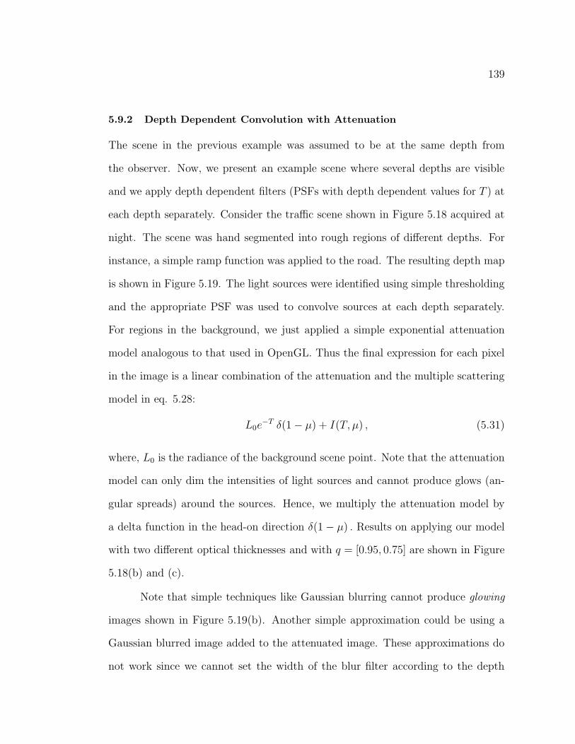
139

5.9.2 Depth Dependent Convolution with Attenuation

The scene in the previous example was assumed to be at the same depth from

the observer. Now, we present an example scene where several depths are visible

and we apply depth dependent filters (PSFs with depth dependent values for T ) at

each depth separately. Consider the traffic scene shown in Figure 5.18 acquired at

night. The scene was hand segmented into rough regions of different depths. For

instance, a simple ramp function was applied to the road. The resulting depth map

is shown in Figure 5.19. The light sources were identified using simple thresholding

and the appropriate PSF was used to convolve sources at each depth separately.

For regions in the background, we just applied a simple exponential attenuation

model analogous to that used in OpenGL. Thus the final expression for each pixel

in the image is a linear combination of the attenuation and the multiple scattering

model in eq. 5.28:

L0e−T δ(1 − µ) + I(T, µ) , (5.31)

where, L0 is the radiance of the background scene point. Note that the attenuation

model can only dim the intensities of light sources and cannot produce glows (an-

gular spreads) around the sources. Hence, we multiply the attenuation model by

a delta function in the head-on direction δ(1 − µ) . Results on applying our model

with two different optical thicknesses and with q = [0.95, 0.75] are shown in Figure

5.18(b) and (c).

Note that simple techniques like Gaussian blurring cannot produce glowing

images shown in Figure 5.19(b). Another simple approximation could be using a

Gaussian blurred image added to the attenuated image. These approximations do

not work since we cannot set the width of the blur filter according to the depth

140

of scene point in a physically consistent manner. Ad hoc methods could be tried

requiring time consuming human intervention, but note here that our method pro-

vides an accurate physics-based way of setting parameters of the model taking into

account the depths of light sources.

5.9.3 Depth Dependent Convolution with Attenuation and Airlight

The third scene we demonstrate is a scene photographed in the evening with deco-

rative lights on trees. In this case, we took into account environmental illumination

(due to the sky) in addition to the attenuation model and the multiple scattering

model mentioned above. The sky was assumed to be overcast. The scattering due

to skylight, called airlight [61], was assumed to be mainly single scattered. The

simple attenuation plus airlight model was then applied to the original photograph

according to a rough depth segmentation of the scene. The final expression used

to render these images is as follows:

[L0e−T + Lsky(1 − e−T )] δ(1 − µ) + I(T, µ) , (5.32)

where Lsky is the horizon brightness [86]. As in the second example, we multiply

attenuation and airlight by a delta function in the head-on direction.

Two different amounts of mist and fog (q = [0.8, 0.9], minimum T = [1.05, 2.0])

were added to the image in Figure 5.20(a). These results are illustrated in Figures

5.20(c) and (d). Note the glowing appearance of the trees and also that the extent

of the glows vary with the distance of the trees from the observer. Further, compare

our technique with only single scattering shown in Figure 5.20(b). The results in

Figure 5.18 and Figure 5.17 indicate that our technique suffices to produce high

quality images without noticeable artifacts, and that single scattering on its own

cannot produce any glows. Each simulation took less than a minute using Matlab

141

Figure 5.18: On the left is a real photograph of a traffic scene on a clear night. Thenext images show the effects of mist and fog (with different atmospheric visibilities)added interactively using our analytic model for multiple scattering from light sources.Notice the glows around the sources (street lamps, car headlights and advertisementsigns) and that the brightnesses and extents of these glows depend on the depths of scenepoints. Simple approximations like Gaussian blurs, single scattering or diffusion cannotaccurately model these complex multiple scattering effects. The slight reddish tinge seenin the images are due to the reddish response of the CCD in the sensor we used.

Figure 5.19: On the left, roughly segmented depth map of the scene in Figure 5.18. Theroad is modeled using a simple ramp (linear) function. Brighter values denote fartherscene points. On the right, Gaussian blurring with different widths (proportional toscene depth) applied to each depth separately. Note that such operations cannot producerealistic glows around light sources in photographs. Compare the Gaussian blurred imageto the more realistic images in Figures 5.18(b) and (c) generated using our model.

142

(a) Original Photograph (f) Airlight + Attenuation model (min T = 1.05)

(c) Mild Mist (q = 0.8, min T = 1.05) (d) Dense Fog (q = 0.9, min T = 2.0)

Figure 5.20: Decorative lights on trees glowing in fog and mist. (a) Original Photograph.(b) Foggy image rendered using single scattering (airlight + attenuation models). (c) and(d) Glows are added to lights on the trees. Note that multiple scattering effects due tolight sources are significant as compared to single scattering effects.

potentially making the method interactive.

In summary, our method for adding weather effects to images is physically-

based, fast (near real-time), produces much better results than current approxi-

mations like diffusion, blurring and single scattering, and at the same time, the

implementation is very simple.

143

5.10 Inverse Problem in Spherical Radiative Transfer

Consider purely scattering media (W0 = 1). For example, light absorption is min-

imal in atmospheric conditions in the visible wavelength range. In this scenario,

our solution reduces to a 2 parameter (T, q) function. Then, the estimation of the

medium parameters (T, q) from the observed scattered light field I(T, µ), at a sin-

gle optical thickness T along various directions µ, can be posed as a 2 parameter

non-linear optimization problem. In this section, we describe what the appearance

of a light source in the atmosphere reveals about the scene, the sources and the

atmosphere itself.

5.10.1 Recovering Source Shape and Atmospheric PSF

Consider an image of an area source in bad weather. From (5.30), we see that

the simultaneous recovery of the APSF and the clear night view of the source

(I0S) is ill-defined. However, under certain conditions, the shape of the source S

can be roughly detected despite the glow around it. Note that any APSF has a

peak at the center that is mainly due to the light scattered in the direction of the

camera (θ = 0). If this peak has much higher value than the values of neighboring

directions, the actual source location in the image can be roughly detected using

thresholding or high pass filtering. Figure 5.21 shows simulations of an actual coil

shaped lamp under mild weather conditions. We conclude that it is easier to detect

shapes in rain than in fog, haze or weather conditions arising due to small aerosols.

An approach for recovering source shape, and hence for removing the glow

around the source, is to use the APSF computed from real data. Images of two

sources with different radiant intensities, shown in Figure 5.22(a) and (d), were

captured on the same night. These sources were adjacent to one another (same

144

(a) Clear image (b) Rainy image (c) Foggy image

(d) Hazy image (e) Image through small aerosolsFigure 5.21: When can source shapes be detected? (a) Clear image of a coil shapedsource. APSFs of different weather conditions with the same optical thickness, are appliedto this source to obtain their glow appearances. (b) Shape can be roughly detected. (c)-(e) Hard to detect source shape.

depth from the camera), and hence they share the same APSF, normalized to [0−1].

We applied a simple thresholding operator to the image in Figure 5.22(a) to obtain

the shape S. We assumed that the radiant intensities I0 of the source elements are

constant across the area of the source and then recovered the normalized APSF

using:

APSF = I ∗ (I0S)−1 . (5.33)

The normalized APSF was used to deconvolve the image of the second source (an

electronic billboard) and remove the glow around the second source.

In the above discussion, it was assumed that the sensor PSF is a delta func-

tion. However, limitations of the sensor optics introduces a non-delta PSF. In all

cases, therefore, the images must be deconvolved by the sensor PSF. The sensor

PSF can be obtained either by capturing an image of a distant source (or speck)

that projects to a single pixel or by using resolution charts. The sensor optics must

145

−100 −50 0 50 1000

0.2

0.4

0.6

0.8

1APSF

Pixel

(a) (b) (c)

(d) (e)Figure 5.22: Shape detection, APSF computation, and glow removal. Two adjacentsources (a) and (d) of different shapes and intensities imaged under rainy and mistyconditions. (b) The shape of the source in (a) is detected using simple thresholding. (c)The APSF of the source in (a) is computed using (5.33). (e) The APSF shown in (c) isused to remove the glow around the electronic billboard (d).

be such that the PSF of the sensor does not kill the frequencies in the atmospheric

PSF. Fortunately, since multiple scattering is a smoothing phenomenon, several

good lenses PSFs do not block any APSF frequencies. In our experiments, we used

a high quality Nikon AF Nikkor Zoom Lens.

5.10.2 From APSF to Weather

In this section, we explore how our model for the APSF can be used to recover the

depth of the source as well as information about the atmosphere. The APSF (5.28)

depends on two quantities: (a) optical thickness T , which is scaled depth, and (b)

forward scattering parameter q of the weather condition. The optical thickness T

is related to the visibility V in the atmosphere and distance R to the source as [75]:

T = σR ≈ 3.912

VR . (5.34)

146

Furthermore, the value of the forward scattering parameter q can be used to find the

type of weather condition (see Figure 5.6). Given an APSF, it is therefore desirable

to estimate the model parameters T and q. The APSF can either (a) be directly

measured from the image (as in Figure 5.11) when the source image lies within a

pixel, or (b) be computed from the image as described in section 5.10.1, when the

image of the source is greater than a pixel. We then use a standard optimization

tool to estimate the APSF model parameters, T and q, that best fit the measured

or computed APSF.

5.10.3 A Visual Weather Meter

The ability to compute the type of weather and the visibility of the atmosphere

from one image of a distant source turns a camera into a “Remote Visual Weather

Meter”. We performed extensive experiments to test the accuracy of our tech-

niques. We used images (Figure 5.23(a)) of a real light source acquired under 45

different atmospheric conditions. These light source images were obtained from the

Columbia University Weather and Illumination Database (WILD) [89]. We also

obtained the ground truth weather data (type and visibility) as well as the actual

depth of the source from the sensor, from the database.

The APSF and its parameters - optical thickness T and forward scattering

parameter q were computed as described before, for each of the 45 conditions. Using

the estimated T and the ground truth depth R, the visibility V was computed from

(5.34). The estimated visibilities follow the trend of the actual visibility curve

(Figure 5.23(b)). Similarly, we used the estimates of T and the ground truth

visibilities V to compute the depth R from (5.34). The resulting depths obtained

in the 45 trials are shown in Figure 5.23(c). The plots are normalized so that the

147

ground truth depth is 1 unit.

The range of estimates for q in the 45 images were between 0.75 and 1.0.

These conformed to the prevalent weather conditions: haze, mist and rain (Figure

5.23(d)). The ground truth weather data from the WILD database was collected

at an observatory three miles away from the location of the source. Hence, some

of the errors in the plots can be attributed to the possible incorrect ground truth

data.

5.11 Summary

We derived an analytic series solution to the radiative transfer from an isotropic

point source immersed in a homogeneous spherical medium. The solution is valid for

both isotropic and non-isotropic scatterers and for both absorbing and purely scat-

tering media. We validated the model extensively using Monte Carlo simulations as

well as real experiments with light sources immersed in milk and the atmosphere.

Unlike computationally intensive numerical simulations, our model can be used to

estimate the radiation field in the medium accurately and instantaneously.

We presented two applications of our model that are relevant to computer

vision and computer graphics. The model we developed can be used for real-

time rendering of sources in various participating media. The model was further

exploited to compute scaled depth, visibility, and the type of weather condition,

from a single image of a source at night. This allowed a camera to serve as a

“visual weather meter”. In future work, we wish to extend our analysis to radiative

transfer from non-isotropic sources and apply the model to several problems in

medical imaging, underwater imaging and remote sensing.

148

(a) A real light source viewed under 45 different atmospheric conditions.

5 10 15 20 25 30 35 40

1

2

3

4

5 Ground Truth Visibilities Computed VisibilitiesMiles

Time

45

(b) The accuracy of computed visibilities.

5 10 15 20 25 30 35 40 45

0.5

1

1.5

2 Ground Truth Depth Estimated Depth

Time

Error

0

(b) The accuracy of computed depth.

0 5 10 15 20 25 30 35 40 45Snow

Haze

Mist

Rain

Time

GroundtruthEstimated

(b) The accuracy of the computed weather condition.

Figure 5.23: A Visual Weather Meter: (a) A light source of known shape is observedunder a variety of weather conditions (rain, mist, haze, snow) and visibilities (1 mile to5 miles). Optical thickness T and forward scattering parameter q are computed fromthe glow observed in each image. (b) Actual ground truth depth is used to compute thevisibility (see (5.34)). (c) To calculate depth, we used the ground truth visibilities and thecomputed T (see (5.34)). (d) Weather conditions recovered from all images. Empty circledenotes a mismatch between estimated and ground truth weather condition. The imagesof the sources and ground truth data were taken from the Columbia WILD database [89].

Part IV

Weather and Illumination

Database

149

151

Chapter 6

WILD: Weather and ILlumination

Database

6.1 Variability in Scene Appearance

The appearance of a fixed scene depends on several factors - the viewing geometry,

illumination geometry and spectrum, scene structure and reflectance (BRDF or

BTF) and the medium (for example, atmosphere) in which the scene is immersed.

The estimation of one or more of these appearance parameters from one or more im-

ages of the scene has been an important part of research in computer vision. Several

researchers have focused on solving this inverse problem under specific conditions

of illumination (constant or smoothly varying), scene structure (no discontinuities),

BRDF (lambertian) and transparent media (pure air). Images captured to evaluate

their methods adhere to the specific conditions. While understanding each of these

specific cases is important, modeling scene appearance in the most general setting

is ultimately the goal of a vision system.

152

To model, develop and evaluate such a general vision system, it is critical to

collect a comprehensive set of images that describes the complete variability in the

appearance of a scene. The light field [35] or the plenoptic function [2] is a function

of all the appearance parameters mentioned above and thus, fully describes scene

appearance. Levoy and Hanrahan [66] and Gortler et al., [38] have measured the

light fields around toy objects, as a coarse 4D sampling. Sampling the entire light

field over a substantial period of time, however, is extremely costly.

Several research groups have collected images of a scene (for example, faces,

textures, objects) under varying lighting conditions and/or viewpoints in controlled

lab environments. The CMU-PIE database [121] has 40000 facial images under

different poses, illumination directions and facial expressions. The FERET [106]

database consists of 1196 images of faces with varying facial expressions. Similarly,

the Yale Face database [9] has around 165 images taken under different lighting,

pose and occlusion configurations. The SLAM database [80] provides a set of 1500

images of toy objects under different poses. The color constancy dataset collected

by Funt et al. [31] provides a large set of images of objects (boxes, books and

so on) acquired under different poses and with different illuminants (fluorescent,

halogen, etc). The CURET database [23] provides a set of 12000 images of real

world textures under 200 illumination and viewing configurations. It also provides

an additional set of 14000 Bi-directional Texture Function (BTF) measurements of

61 real world surfaces.

Several databases of images of outdoor scenes have also been collected. The

“natural stimuli collection” [134] has around 4000 images of natural scenes taken on

clear, foggy and hazy days. Parraga et al. [103] provide a hyper-spectral dataset of

153

29 natural scenes. The MIT city scanning project [130] provides a set of 10000 geo-

referenced calibrated images acquired over a wide area of the MIT campus. These

databases, however, do not cover the complete appearance variability (due to all

outdoor illumination and weather conditions) in any one particular scene. Finally,

web-cams [41] used for surveillance capture images regularly over long periods of

time. However, they are usually low quality, non-calibrated, not tagged with ground

truth data and focus only on activity in the scene. Note that the references we have

provided for various databases are by no means complete. We refer the reader to

[20] for a more comprehensive listing.

In this chapter, we present a set of very high quality registered images of

an outdoor scene, captured regularly for a period of 9 months. The viewpoint (or

sensor) and the scene are fixed over time. Such a dataset is a comprehensive collec-

tion of images under a wide variety of seasons, weather and illumination conditions.

This database serves a dual purpose; it provides an extensive testbed for the eval-

uation of existing appearance models, and at the same time can provide insight

needed to develop new appearance models. To our knowledge, this is the first effort

to collect such data in a principled manner, for an extended time period.

We begin by describing the image acquisition method, the sensor calibra-

tion procedures, and the ground truth data collected with each image. Next, we

illustrate the various factors that effect scene appearance using images from our

database captured over 9 months. Several experiments and evaluations in the pre-

vious chapters have been performed on the images of this dataset. In addition

to computer vision, this database has potential implications for graphics, image

processing as well as atmospheric sciences.

154

6.2 Data Acquisition

In this section, we describe the camera we used to acquire images, the collection

setup and the quality and quantity of images we capture.

6.2.1 Scene and Sensor

The scene we image is an urban scene with buildings, trees and sky. The distances

of these buildings range from about 20 meters to about 5 kilometers. The large

distance range facilitates the observation of weather effects on scene appearance.

See Figure 6.4 for the entire field of view. The digital camera we use for image

capture is a single CCD KODAK Professional DCS 315 (see Figure 6.1) [56]. As

usual, irradiance is measured using 3 broadband R, G, and B color filters. An AF

Nikkor 24 mm - 70 mm zoom lens is attached to the camera.

6.2.2 Acquisition Setup

The setup for acquiring images is shown in Figure 6.1. The camera is rigidly

mounted over a pan-tilt head which is fixed rigidly to a weather-proof box (see

black box in Figure 6.1). The weather-proof box is coated on the inside with two

coats of black paint to prevent inter-reflections within the box. An anti-reflection

glass plate is attached to the front of this box through which the camera views

the scene. Between the camera and the anti-reflection plate, is a filter holder (for,

say, narrow band spectral filters). This box has two side doors and a back door

for access to within the box (say, for cleaning purposes or to change filters). The

entire box with the camera and the anti-reflection glass plate is mounted on a panel

rigidly attached to a window. The camera is connected to a 450 MHz Pentium III

computer through the standard IEEE 1394 firewire interface. The images captured

by the camera are directly stored in the computer hard drive.

155

Anti-reflection Glass

Kodak DCS315

10-bit Camera

24 -70 mm Zoom LensPan/Tilt Stage

Weather Proof

Enclosure

FireWire (IEEE 1394)

Figure 6.1: Acquisition Setup

6.2.3 Image Quality and Quantity

Images are captured automatically every hour for 20 hours each day (on an average).

The spatial resolution of each image is 1520×1008 pixels and the intensity resolution

is 10 bits per pixel per color channel. Currently, we have acquired images for over

150 days. In total, the database has around 3000 images. Due to maintenance issues

that arise from prolonged camera usage (camera power failures and mechanical

problems in controlling camera shutter), we have had to remove the camera twice

from the enclosure. We believe the resulting loss of few days in the database can

be tolerated since the dataset has enormous redundancy. The new image sets are

registered with existing ones using the Matlab image registration utility.

To capture both subtle and large changes in illumination and weather, high

dynamic range images are required. So, we acquire images with multiple exposures

(by changing the camera shutter speed while keeping the aperture constant) and

apply prior techniques to compute a high dynamic range image (≈ 12 bits per pixel)

of the scene. Since the illumination intensity is expected to vary with time, the set

of exposures are chosen adaptively. First, an auto-exposure image is taken and its

shutter speed is noted. Then 4 more images are captured with exposures around

this auto-exposure value. This type of adaptive exposure selection is commonly

used by photographers and is called exposure bracketing.

156

(a) High Exposure (b) Auto Exposure ( c) Low Exposure

(d) Radiometric Response (e) Computed High Dynamic Range Image (Histogram Equalized)

RG

B

I

M

0

1

0.5

0 10.5

ImageIrradiance

MeasuredIntensity

1 2

3

1 2

3 1

Figure 6.2: Radiometric Self-Calibration. (a) - (c) Three images (10 bits per pixelper RGB channel) captured with different camera exposures. (d) Computed radiometricresponse functions of the 3 RGB channels. The response functions are linear with slopes1.5923, 1.005 and 0.982 for R, G, and B respectively. The colors can be balanced bynormalizing the slope of each response function. (e) Histogram equalized high dynamicrange image irradiance map obtained by combining images taken with multiple exposures.Insets indicate that the dynamic range in this image is much higher than the dynamicrange in any image captured using a single exposure.

6.3 Sensor Radiometric Calibration

Analysis of image irradiance using measured pixel brightness requires the radiomet-

ric response of the sensor. The radiometric response of a sensor is the mapping, g,

from image irradiance, I, to measured pixel brightness, M : M = g(I) . Then, the

process of obtaining I from M : I = g−1(M) , up to a global scale factor, is termed

as radiometric calibration.

The response functions of CCD cameras (without considering the gamma or

color corrections applied to the CCD readouts) are close to linear. We computed

the response functions of the 3 RGB channels separately using Mitsunaga and

Nayar’s [78] radiometric self-calibration method. In this method, images captured

with multiple exposures and the their relative exposure values are used to estimate

the inverse response function in polynomial form. The results of the calibration

157

are shown in the plots of Figure 6.2(d). Notice that the response functions of

R, G, and B are linear and they have different slopes - 1.5923, 1.005 and 0.982

respectively. To balance the colors, we normalize the response functions by the

respective slopes. The images taken with different exposures are linearized using

the computed response function. A high dynamic range image irradiance map (see

Figure 6.2) is obtained by using a weighted combination of the linearized images.

This image has significantly more dynamic range then any of the original images

taken with single exposures [95]. The high dynamic range can prove very useful

when analyzing both subtle and large changes in weather and illumination.

6.4 Ground Truth Data

Any database is incomplete without the accompanying ground truth. We have

tagged our images with a variety of ground truth information. Most important

categories of the ground truth we collected are scene depth and weather information.

The depths of scene points are mainly obtained using satellite digital orthophotos

supplied by the United States Geological Survey [133]. Arcview [29] is a mapping

software that is used to measure the orthographic distance between two scene points

(visible in the orthophotos) up to an accuracy of 1 meter. See Figure 6.3 for an

example of a satellite orthophoto. Note that accurate depth is not available at all

pixels. However, since the field of view consists of mainly vertical buildings, rough

planar models can be used.

The position (longitude, latitude and altitude) of the sensor is included in

the database. This information along with the date and time of day, can be used

to accurately compute sun and moon orientation relative to the sensor. For exact

equations, see [7; 93].

158

Conditions at 2001.03.06 11:51am

Wind NNW (340 ) 10 MPH

Visibility 1 1/4 mile(s)

Sky conditions Overcast

Weather Light snow, Mist

Precipitation last hour A trace

Temperature 32.0 F (0.0 C)

Dew Point 32.0 F (0.0 C)

Relative Humidity 100%

O

FOV

Figure 6.3: Sample ground truth data. [Left] A satellite digital orthophoto of a portionof the scene. The red spot indicates the position of the sensor and bright region indicatesthe field of view. Arcview [29] is used to measure the orthographic distance between anytwo scene points (seen in top view) with an accuracy of 1 meter. [Right] The weatherdata obtained from National Weather Service websites [99].

Every hour we automatically collect standard weather information from the

National Weather Service web sites [99]. This includes information about sky con-

dition (sunny, cloudy), weather condition (clear, fog, haze, rain), visibility, temper-

ature, pressure, humidity and wind (see Figure 6.3). Such information can be used

to estimate the scattering coefficient of the atmosphere [1].

6.5 Images of WILD

We illustrate the variability in scene appearance due to weather, illumination, sea-

son changes, and surface weathering using images from our dataset captured over

five months.

6.5.1 Variation in Illumination

The distribution of environmental illumination on a scene produces a wide variety

of scene appearances. Commonly noticed effects include shadows, colors of sunrise

and sunset, and illumination from stars and moon at night. The human visual

system relies on illumination in the scene to perceive scene reflectance (retinex and

color constancy [63]) and shape [109] correctly. As a result, rendering a scene with

159

consistent illumination is critical for realism in graphics.

Considerable amount of effort has been put into modeling outdoor illumina-

tion. The book “Daylight and its Spectrum” [43] provides a compendium of color

and intensity distributions of skylight for many years of the 20th century. Daylight

spectrum has also been represented using a set of linear bases [122]. Works that

model clouds and their effect on the ambient illumination also exist in literature [79;

37]. In graphics, scenes have been rendered under different daylight [129] and night

illuminations [52]. Shadows are a powerful cue for shape and illumination per-

ception. Rendering shadows and extracting shape information from shadows [55;

62] are also important problems.

Let us consider the various sources of illumination in any outdoor scene.

The primary sources (self-luminous) include the sun during the day, the stars and

lamps during night. There are numerous other secondary illumination sources such

as skylight, ground light, moonlight, airlight [61] (due to scattering of light by the

atmosphere), and scene points themselves (inter-reflections [94]). Our goal is to

include the effects of all these sources in one comprehensive database. Figure 6.4

shows 6 images from our database illustrating the various shadow configurations on

a sunny day. Figure 6.5 shows different illumination colors and intensities at sunrise,

noon, sunset and night. Figure 6.6 depicts the variations in ambient lighting due

to varying cloud covers.

When viewed up-close, rough surfaces appear to have 3D textures (due to

surface height variations) rather than 2D textures. The appearance of 3D textures

has been modeled in [23]. Figure 6.7 shows the appearance of a rooftop with ridges

at different times of the day. Notice the change in appearance of cast shadows due

160

09/07/2001, 3 PMClear and Sunny

09/07/2001, 10 AMClear and Sunny

09/07/2001, 12 NoonClear and Sunny

09/07/2001, 11 AMClear and Sunny



Figure 6.4: Images illustrating different shadow configurations on a clear and sunnyday. Shadows provide cues for illumination direction and the scene structure. Notice thepositions of the sharp shadows on the buildings.

09/05/2001, 6 AMSun Rise

09 / 05/2001, 10 PMNight

09/05/2001, 7 PMSun Set

09/05/2001, 12 noonNoon

Figure 6.5: Images illustrating the various colors and intensities of illumination at sun-rise, noon, sunset and night. Notice the significant change in the colors of the sky.

to surface height variations.

The above variability in a single database facilitates research groups to study

the illumination effects individually as well as simultaneously. For instance, one

may use just sunny day images at one particular time of day, when the sun position

remains constant and shadows do not change. In another instance, one can consider

images captured only on cloudy days to model scenes under ambient lighting.

161

7 AM, Partly Cloudy, Partly Sunny 7 AM, Increased Cloud Cover 7 AM, Overcast Sky

Figure 6.6: Images showing various levels of cloud cover. The image on the left shows theappearance of the scene with a few scattered clouds. The two images on the right weretaken under mostly cloudy and completely overcast conditions. Notice the soft shadowsdue to predominant ambient lighting.

9 AM 12 Noon 3 PM

Figure 6.7: When viewed at close proximity (fine scale), the appearances of surfacesshould be modeled using the bi-directional texture function (BTF) instead of the BRDF.Notice the change in cast shadows due to the ridges on the rooftop. All images arehistogram equalized to aid visualization.

6.5.2 Variation in Weather Conditions

Since the collection was done for over 9 months, the images of the dataset contain

a wide variety of weather and visibility effects. In this section, we describe some of

the effects seen in the images.

How can the models for weather analysis be evaluated? Under what condi-

tions do these models fail or perform well? To satisfactorily answer such questions,

we must evaluate the performance of such models and algorithms on images of a

scene captured under a wide variety of illumination and weather conditions. Our

database includes images of the scene under many atmospheric conditions including

clear and sunny, fog, haze, mist, rain and snow. Indeed several of our experiments

and evaluations are performed on the images in this database. Figure 6.8 shows 4

images of the same scene captured under different weather conditions. Notice the

162


09/14/2001, 1 PMFoggy

06/14/2001, 1 PMHazy

06/02/2001, 1 PMLight Mist and Rain

Figure 6.8: Images taken at the same time of day but under different weather conditions.Notice the degradation in visibility, especially, of far away scene points in bad weather.

05/28/01, 11 PMClear Night

05/26/01, 11 PMMisty Night

Figure 6.9: Night images showing light sources under clear and misty conditions. Thesources appear like specks of light on a clear night. Notice the light spreading due tomultiple scatterings on a misty night.

significant reduction in contrast (and increase in blurring) in far away buildings.

Broadening of light beams due to multiple scatterings in the atmosphere is clearly

illustrated by the lamps imaged at night (see Figure 6.9).

Consider the event of mild fog setting in before sunrise, becoming dense as

time progresses and finally clearing by noon. We believe that such lengthy, time

varying processes can be studied better using our database. Study of such processes

have potential implications for image based rendering.

163

Summer Season, 06/15/2001, 11 AM Fall Season, 09/15/2001, 11 AM

Figure 6.10: Images taken at the same time of day but on days in summer and fall. Boththe images were taken on clear and sunny days. Notice the subtle differences in colorsand the positions of shadows.

6.5.3 Seasonal Variations

The types of outdoor illumination and weather conditions change with seasons. For

instance, the intensity distribution of sunlight and skylight differ from summer to

winter [43]. Similarly, the atmospheric conditions that manifest in fall are signif-

icantly different from those that occur in winter. Models of the atmosphere and

climate in different seasons can be found in [1] and other related papers [3].

Since we acquire the images for over 9 months, changes in scene appearance

due to changes in seasons can be studied. For instance, one might easily compare

the images taken on a clear day in spring with images taken on a clear day in winter

under identical sensor settings. Figure 6.10 shows 2 images taken at the same time

of day in summer and fall.

6.5.4 Surface Weathering

Over substantial periods of time, we commonly see oxidation of materials (rusting),

deposition of dirt on materials and materials becoming wet or dry. These effects

are important for realistic scene rendering and have been modeled by Dorsey and

Hanrahan [25]. Since our images have high spatial resolution, portions of the image

corresponding to small regions in the scene (say, a portion of a wall) can be analyzed.

Figure 6.11 shows a small patch in the scene when it is dry and wet.

164

Figure 6.11: Portions of a rooftop in the scene when it is dry, partly and completely wet.

6.6 Summary

The general appearance of a scene depends on a variety of factors such as illu-

mination, scene reflectance and structure, and the medium in which the scene is

immersed. Several research groups have collected and analyzed images of scenes

under different configurations of illuminations (both spectrum and direction), and

viewpoints, in controlled lab environments. However, the processes that effect out-

door scene appearance such as climate, weather and illumination are very different

from indoor situations. Ultimately, vision algorithms are expected to work robustly

in outdoor environments. This necessitates a principled collection and study of im-

ages of an outdoor scene under all illumination and weather conditions. We have

collected a large set of high quality registered images of an outdoor urban scene cap-

tured periodically for five months. We described the acquisition process, calibration

processes and ground truth data collected. Several experiments and evaluations in

this thesis are performed on the images from this dataset. We believe that this

dataset has potential implications in vision, graphics and atmospheric sciences.

165

Chapter 7

Conclusions and Future Work

Ultimately, vision systems must be able to handle problems posed by bad weather.

This thesis lays the foundation for scene interpretation in a variety of stable weather

conditions such as fog, mist, haze and other aerosols. We summarized existing

models in atmospheric optics and proposed several new ones, keeping in mind the

constraints faced by most vision applications. In addition, we presented several

algorithms for recovering pertinent scene properties, such as 3D structure, and

clear day scene contrasts and colors, from images taken in poor weather, without

requiring prior knowledge of atmospheric conditions. We also developed algorithms

for recovering useful information about the atmosphere, such as the type of weather

(fog, haze, mist), and the meteorological visibility. In the remainder of this chapter,

we list the contributions of this thesis and describe several areas of future work.

7.1 Summary of Contributions

We now present a summary of the contributions of this thesis. Figures 7.1 and 7.2

show a visual snapshot of the contributions.

166

(b) Output: Dehazed 3D views

I. Color Restoration and 3D Structure

II. Contrast Restoration Irrespective of Scene Distances

(a) Input : Mild haze and Dense haze

(c) Input : Zoomed-in Regions of a Street Scene at Different Depths

(d) Output : Different Amounts of Fog Removed Automatically from Different Distances

(f) Output: Dehazed Image

III. Dehazing Using Polarization

IV. WILD : Weather and Illumination Database

(e) Input : Minimum and Maximum Polarization Images

(g) Clear and Sunny (h) OvercastSky, Mist (i) Night, Dense Fog (j) Overcast Sky, Heavy Rain

Figure 7.1: Visual Snapshot of Thesis Contributions.

167

VI. Rendering Multiple Scattering using Convolution

(b) Two different densities of fog added to image on the left

V. Multple Scattering Model Validated using Experiments with Milk

(b) Apparatus and Images showing glows for different milk concentrations.

Figure 7.2: Visual Snapshot of Thesis Contributions (continued).

7.1.1 Single Scattering Models for Stable Weather

To understand the interaction of light with the atmosphere and its effect on imaging,

we have developed a comprehensive set of physics-based single scattering models

that describe the appearances of scenes under stable weather conditions such as

fog, haze, and mist. These models describe the colors, contrasts and polarizations

of observed scene points under different stable weather conditions.

7.1.2 Structure from Weather

At first glance, bad weather may be viewed as no more than a hindrance to an

observer. However, it turns out that bad weather can be put to good use. The

farther light has to travel from its source (say, a surface) to its destination (say,

a camera), the greater it will be effected by the weather. Hence, bad weather

could serve as a powerful means for coding and conveying scene structure. This

observation lies at the core of our investigation. We have developed 5 algorithms

168

to compute three dimensional scene structure from one or more images of a scene

captured under poor but unknown weather conditions. An example result is shown

in Figure 7.1(a).

7.1.3 Removing Weather Effects from Images and Videos

Bad weather can severely impact the performance of any outdoor vision system.

One approach to overcome bad weather effects is to explicitly remove them from

the images before performing further analysis. We have developed 3 algorithms to

restore clear day contrasts and colors of scene points from images taken under poor

weather conditions. In all these methods, we make no assumption on the types of

reflectances or illuminations on the scene, or the exact types of weather conditions.

Example experimental results are shown in Figures 7.1(a,b,c).

7.1.4 Weather and Illumination Database (WILD)

We have acquired an extensive set of high quality (12 bits per pixel), high resolution

(1520 x 1008) images of a static outdoor scene every hour for over nine months.

This database is the first of its kind and contains images taken under a wide variety

of weather (clear, fog, mist, haze, snow, rain) and illumination (sunny, cloudy, day,

night) conditions as well as all four seasons (fall, winter, spring, summer). Each

image is tagged with a variety of ground truth data about the weather and sky

condition, as well as scene depths obtained from satellite orthophotos. A subset

of images is shown in Figure 7.1(d). We have used the images from the WILD

database for several of our experiments and evaluations. Our WILD database has

been distributed to 50 research groups in North America, Europe and Asia, since

August 2002. We believe this database itself can spawn new research in the fields

of computer graphics, vision, remote sensing and atmospheric sciences.

169

7.1.5 Multiple Scattering around Light Sources

We have developed an analytic model for multiple scattering of light from a light

source immersed in virtually any scattering medium. Using this model, we have

demonstrated fast and accurate rendering of volumetric effects in graphics, and

computation of weather information (meteorological visibility and type of weather

condition) from a single image of a light source and its surrounding glow. We

believe that this model has implications also for medical imaging, underwater and

satellite imaging. We intend to use these results as building blocks for developing

more advanced weather-tolerant vision techniques.

7.1.6 Publications

Parts of the research conducted towards this thesis have been published in various

conferences [96; 90; 85; 84; 116; 89; 88; 87] and journals [91; 117; 92].

7.2 Future Work

This thesis mostly focused on stable or steady weather conditions such as fog, haze,

mist and other aerosols. We believe that a major area of future work could be in

developing models and algorithms for dynamic weather conditions such as rain, hail

and snow and turbulence. The other area where there is a wide scope for future

work is on the fast and accurate rendering of volumetric effects in participating

media in general settings. We describe these areas (along with other smaller areas)

of future work and propose possible (albeit speculative) research directions in these

areas.

7.2.1 Modeling Dynamic Weather Conditions

In steady weather (fog, haze, mist), the individual water droplets that constitute

the weather are too small (1 − 10 µm) to be individually detected by a camera.

170

The intensity at a pixel in stable weather is due to the aggregate effect of a large

number of these drops within the pixel’s solid angle. Hence, volumetric (aggregate)

models of atmospheric scattering, such as attenuation and airlight, can be used to

adequately describe the effects of stable weather.

On the other hand, dynamic weather conditions, such as rain and snow,

produce much more complex visual effects. Rain drops are large enough (1 −10 mm) to be individually detected by the camera. Furthermore, their motions

produce randomly varying spatial and temporal intensities in an image. Aggregate

scattering models will not suffice to model the random spatio-temporal fluctuations

caused by dynamic weather conditions. Thus, stochastic models may be more

effective for handling dynamic weather. Most of this discussion was adapted from

[33; 32].

7.2.2 Handling Non-Homogeneous Weather

One of the assumptions made in this thesis is that the atmosphere (or the scattering

medium) is homogeneous. This approximation is valid for short distance ranges (a

few kilometers) and more or less horizontal lines of sight. However, for large distance

ranges (for example, as in remote sensing) or near vertical lines of sight (for example,

as in satellite and telescopic imaging), this assumption is violated. In general, we

expect that it may be possible to compute optical thickness but it will be hard

to compute scene structure under arbitrary (and unknown) homogeneities. The

optical thicknesses so computed need to be used to remove weather effects. As an

example, consider a simpler type of non-homogeneity (homogeneous in X-Y plane

but non-homogeneous along the Z axis (line of sight)). In this case, it is possible to

compute optical thickness and remove weather effects using the polarization-based

171

model and algorithms. Future work includes generalizing this to more interesting

non-homogeneities.

7.2.3 What can be known from a Single image?

Most of our algorithms to compute structure required two images taken under vary-

ing atmospheric conditions or taken by varying optical settings of the camera. The

structure computed then was used to remove weather effects from an image. Fur-

thermore, we presented depth heuristics to interactively deweather a single image.

Along these lines, it will be interesting to investigate the possibility of deweath-

ering a single image using other types of heuristics or priors on scene colors (for

instance, priors obtained from natural image statistics literature) and sky colors

(for instance, priors obtained from daylight spectral distributions).

7.2.4 Implicit approach to overcome weather effects

Ultimately, any vision system must overcome weather effects in order to perform

more robustly in bad weather. In the explicit approach discussed in this thesis,

we first remove weather effects from input images/videos using physics-based algo-

rithms to obtain clear day images. Further tasks (say, tracking, identification, etc)

may be then performed using the deweathered images. On the other hand, implicit

methods simultaneously use physics-based models and constraints for image under-

standing in bad weather, as well as the task that a particular vision system does

normally. This approach can be task dependent and hence can be more involved

when compared to the explicit approach. However, it can provide significant flex-

ibility in designing robust measures to overcome weather effects and at the same

time perform the required task. Furthermore, in real-time tasks, where applying

an explicit method is computationally expensive, faster implicit methods may be

172

necessary. Design of implicit methods for a variety of vision tasks (say, tracking,

identification, etc) is an important direction for future work.

7.2.5 Analytic Volumetric Rendering in General Settings

Our analytic model for multiple scattering was developed for somewhat restrictive

situations. We now present a series of research problems that we feel are necessary

to achieve rendering volumetric effects due a variety of media in general situations.

At a high level, these research problems can be categorized into (a) new analytic

models and approximations; and (b) new algorithms for fast rendering of volumetric

effects.

Analytic Bases for Variations of the Spherical RTE: In this thesis, we de-

veloped analytic bases (Legendre polynomials) for multiple scattering from a point

light source placed at the center of a spherical medium. Future work includes the

derivation of similar analytic bases for simple variations on the spherical RTE con-

figurations of medium and source geometry. For instance, what happens when the

source is not at the center of the medium but rather at a different location inside

or outside the medium? Then, the light field also depends on the azimuthal angle

from the radius vector. In this case, we believe that using spherical harmonics

enables us to capture the multiple scattering within this volume.

Analytic approximation for Visibility of Sources: In our analytic model, we

assumed that an isotropic point source is immersed in a spherical medium with no

other objects or occluders. In reality, the source could be occluded by nearby objects

or could be non-isotropic. Areas of darkening may be seen in the medium where

the occluders cast shadows. This is a hard problem to solve analytically. However,

we believe that certain analytic approximations can be obtained. For instance, to

173

darken the areas in the shadow region, we may place negative isotropic sources in

the interior of the occluder so as to create the right area of darkening. To handle

non-isotropic sources, we need to consider only a source obtained by blocking a

finite solid angle of an isotropic source. Note that an arbitrary non-isotropic source

could be constructed from smaller solid angles of isotropic sources.

Guiding Monte Carlo Ray Tracers using Analytic Models: One of the

main problems of Monte Carlo approaches to rendering volumetric effects is that

they are computationally very expensive. Their computation cost depends on the

parameters of the medium (say, the volume of the medium and the density of

particles in the medium). In other words, the time required to render an image

of a scene in dense fog could be several orders of magnitude greater than the time

required to render the same scene in mild fog. Also, the time required to render

a larger (scaled) version of the same scene with the same particle density could

be orders of magnitude higher. Thus, rendering scenes by interactively changing

parameters of the scene (be it parameters of the medium or the objects in the scene

itself) can be more or less ruled out. On the positive side, Monte Carlo methods can

accurately take into account arbitrary source and medium configurations, complex

visibility effects as well as arbitrary source radiance distributions.

We propose the use of our analytic models and approximations to guide

Monte Carlo techniques to faster and more accurate convergence. Note that, at

a basic level, the monte carlo method is a randomized technique that numerically

computes complex integrals. Millions of function evaluations are needed for accu-

rate results. We believe that our analytic models will provide starting estimates

that are very close to the final solution in most cases. Thus, the hard dependence

174

of Monte Carlo on the parameters of the scene is alleviated. Also, we can take

advantage of the flexibility in Monte Carlo to render subtle effects due to complex

scenes, that are not captured using the analytic models. This hybrid method enjoys

the advantages of both the techniques.

Using the above set of models and algorithms, it may be possible to ren-

der a wide variety of volumetric effects (atmospheric, underwater, subsurface, etc)

efficiently as well as accurately in general settings.

Part V

Appendices

175

177

Appendix A

Direct Transmission under

Overcast Skies

We present an analysis of the effect of sky illumination and its reflection by a scene

point, on the direct transmission from the scene point. For this, we make two

simplifying assumptions on the illumination received by scene points. Usually, the

sky is overcast under foggy conditions. So we use the overcast sky model[37][136] for

environmental illumination. We also assume that the irradiance of each scene point

is dominated by the radiance of the sky, and that the irradiance due to other scene

points is not significant. See Langer and Zucker’s work[64] for a related analysis.

Consider the illumination geometry shown in figure (A.1). Let P be a point

on a surface and n be its normal. We define the sky aperture Ω of point P , as the

cone of sky visible from P . Consider an infinitesimal patch of the sky, of size δθ

in polar angle and δφ in azimuth as shown in figure (A.1). Let this patch subtend

a solid angle δω at P . For overcast skies, Moon[79] and Gordon[37] have shown

that the radiance of the infinitesimal cone δΩ, in the direction (θ, φ) is given by

178

δθ δφ

P

n

δω

Ω

Sky

Figure A.1: The illumination geometry of a scene point P with surface normal n. Theirradiance of P is due to the airlight radiance of its sky aperture Ω.

L(θ, φ) = L∞(λ)(1 + 2cosθ)δω, where δω = sinθ δθ δφ. Hence, the irradiance at P

due to the entire aperture Ω, is given by

E(λ) =∫ ∫

ΩL∞(λ) (1 + 2cosθ) cosθ sinθ dθ dφ , (A.1)

where cosθ accounts for foreshortening[46]. If R is the BRDF of P , then the

radiance from P toward the observer can be written as

L0(λ) =∫ ∫

ΩL∞(λ) f(θ) R(θ, φ, λ) dθ dφ , (A.2)

where f(θ) = (1 + 2cosθ) cosθ sinθ. Let σ be the projection of a unit patch around

P , on a plane perpendicular to the viewing direction. Then, the radiant intensity

of P is given by I0(λ) = σ L0(λ) . Since L∞(λ) is a constant with respect to θ and

φ, we can factor it out of the integral and write concisely as

I0(λ) = L∞(λ) η(λ) , (A.3)

where

η(λ) = σ∫ ∫

Ωf(θ) R(θ, φ, λ) dθ dφ . (A.4)

179

The term η(λ) represents the sky aperture and the reflectance in the direction of

the viewer. Substituting for I0(λ) in the direct transmission model in (2.6), we

obtain

E(d, λ) = gL∞(λ) η(λ) e−β(λ)d

d2, (A.5)

where g represents the optical setting of the camera (exposure, for instance). We

have thus formulated the direct transmission model in terms of overcast sky illu-

mination and the reflectance of the scene points.

180

Appendix B

Illumination Occlusion Problem

In deriving the expression for the radiance due to airlight in section 2.2.3, we as-

sumed that the atmosphere is illuminated uniformly regardless of the type of illumi-

nation. This is not always true since not all points in the atmosphere “see” the same

solid angle of the sky. In fact, the scene itself occludes part of the sky hemisphere

visible to a point in the atmosphere. For explanation purposes, consider a scene

with a single building. The solid angle subtended at any point in the atmosphere

by the sky is called its sky aperture. As seen in figure B.1, this solid angle decreases

as the distance increases from the observer for any given pathlength. Similarly, the

solid angle is smaller for points near the bottom of the building.

We now present a simplified analysis of this effect. We assume that the

atmosphere is illuminated mainly by overcast skylight (ground light is ignored here).

Then, the irradiance received by any point in the atmosphere is given by (see

equation (A.1)),

E = E(hemisphere) − E(occluded) ,

181

Decreasing Sky Aperture

Dec

reas

ing

Sk

yA

per

ture

Skylight

Sky Aperture

Observer

OccludingScene

Atmosphericparticle

Figure B.1: The scene occludes the sky aperture of points in the atmosphere. As a resultpoints in the atmosphere are not uniformly illuminated by the sky.

E(occluded) =∫ φ

−φ

∫ θ

0L∞ (1 + 2cosθ) cosθ sinθ dθ dφ ,

E(hemisphere) =∫ π

−π

∫ π/2

0L∞ (1 + 2cosθ) cosθ sinθ dθ dφ , (B.1)

where E(hemisphere) is the irradiance the point would receive from the entire sky

hemisphere (as if there were no occlusions). Eoccluded is the irradiance the point

would have received from the occluded part. θ and φ denote the polar and azimuth

of the occluded region. The above equation simplifies to

E = L∞7 π − 7 φ cos2θ (3 + 4cosθ)

3. (B.2)

To correct for the radiance of airlight in section 2.2.3, we multiply by the fraction

of irradiance received by each point and rewrite the airlight radiance (2.13) of a

182

pathlength d as

L(d , λ) = k( 1 − e−β(λ)d ) −∫ d

0k

(φ cos2θ (3 + 4cosθ)

π

)β(λ) e−β(λ)x dx .

(B.3)

Note here that both θ and φ depend on the depth from the observer x (see

figure B.1). In other words, the integral in the previous equation depends on the

exact extent of occlusion by the scene. In our experiments, we have assumed uni-

form illumination of the atmosphere and thus some of the errors in the depth maps

can be attributed to this effect.

183

Appendix C

Sensing with a Monochrome

Camera

In this section, we derive an expression for the intensity E, of a scene point under

bad weather, recorded by a camera within a narrow wavelength band (λ, λ + δλ).

From (2.17) we write,

E =∫ λ+δλ

λs(λ) (Edt(d, λ) + Ea(d, λ)) dλ (C.1)

where s(λ) is the spectral response of the camera. We assume that the scattering

coefficient β does not change appreciably over the narrow spectral band and write,

E =e−βd

d2

∫ λ+δλ

λE∞(λ)s(λ)r(λ)dλ . . .

+ (1 − e−βd)∫ λ+δλ

λE∞(λ)s(λ)dλ (C.2)

The sky illumination spectrum can be written as,

E∞(λ) = I ′∞E∞(λ) , (C.3)

184

where, I ′∞ is the magnitude of the sky illumination spectrum and E∞(λ) is the

normalized sky illumination spectrum. Letting

g =∫ λ+δλ

λE∞(λ)s(λ)dλ ,

ρ =1

gd2

∫ λ+δλ

λE∞(λ)s(λ)r(λ)dλ ,

I∞ = I ′∞ g (C.4)

we rewrite the final brightness at any pixel as,

E = I∞ ρ e−βd + I∞ (1 − e−βd) , (C.5)

where, I∞ is termed as sky intensity. Note that ρ is a function of normalized

sky illumination spectrum, scene point reflectance and the spectral response of the

camera, but not the weather condition β. The algorithm we present in the paper

recovers ρ for each pixel to restore scene contrast.

We now discuss under what weather conditions can this model be applied

to various sensors. Let us now examine the wavelength range in which this model

can be applied. By changing the limits of integration to [λ1, λ2], and assuming the

scattering coefficient to be constant over this wavelength band, we can use the same

model for a black and white camera (entire visible range), or smaller color bands

(R,G,B) for a color camera, or narrow band multi-spectral cameras.

Recall that the scattering coefficient for fog and dense haze remains more

or less constant over the visible spectrum. Accordingly, a broad band RGB or

gray-scale camera suffices to analyze images taken in fog and dense haze. For other

aerosols such as mild haze, multi-spectral cameras or cameras fitted with narrow

band filters should be used in order to apply our methods satisfactorily. Finally,

185

scattering coefficients of most weather conditions vary significantly in the near-

IR spectrum [136] and hence, narrow-band IR cameras have to be used for the

analysis beyond the visible wavelengths. In other words, the greater the variation

in the scattering coefficient with respect to wavelength, the narrower the spectral

bandwidth needed for effective results.

186

Appendix D

Computing I‖ and I⊥

By rotating the polarizer to achieve an extremum of the intensity or contrast (I‖ and

I⊥), it is often easy to visually detect the states corresponding to these components.

However, it is easier and more accurate to estimate these components using three

or more images taken through different general orientations of the polarizer. This

is a common practice in polarization imaging [113; 115; 120; 124; 137].

Let θ‖ be the orientation of the polarizer for best transmission of the com-

ponent parallel to the plane of incidence (see figure 2.7). For a general orientation

α, the observed intensity at each pixel is

I(α) = (1/2)Itotal − a cos[2(α − θ‖)] (D.1)

where a is the amplitude of the modulation caused by changing the filter’s orienta-

tion.

We can write equation (D.1) for an angle αk as

187

[1/2 − cos(2αk) − sin(2αk)]

Itotal

acos

asin

= Ik , (D.2)

where acos = a cos(2θ‖) and asin = a sin(2θ‖). To obtain the estimates Itotal, acos

and asin, three linearly independent measurements are sufficient. If we have more

than 3 measurements, we derive the least squares estimates. Then, we find the

image components as

I‖ = (1/2)Itotal − a (D.3)

and

I⊥ = (1/2)Itotal + a , (D.4)

where a =√

a2cos + a2

sin . These equations also yield an estimate of θ‖ at each

pixel:

θ‖ = (1/2) arctan(asin/acos) . (D.5)

The images shown in figure 3.17 were actually estimated this way, based

on photographs taken at 4 different polarizer orientations. The photographs were

linearized to compensate for the detector’s radiometric response. The response

was estimated from images of the Macbeth ColorChecker [36]. We obtained high

dynamic range images by weighted averaging of multiple exposures.

188

Appendix E

Dehazing using Two Arbitrary

Images

In dehazing images, we used estimates of I‖ and I⊥ in the dehazing algorithm. We

now show that in theory the method can work based on two images taken at almost

any different polarization orientations. Let θ‖ be the orientation of the polarizer

for best transmission of the component parallel to the plane of incidence. For a

general orientation α, the observed airlight is

A(α) = A1 − P cos[2(α − θ‖)]

/2 , (E.1)

which coincides with equations (2.34,2.37) if α = θ‖, θ‖ +90o. Suppose we take two

images of the scene with arbitrary orientations of the polarizer, α1 = α2. Because

the direct transmission is unaffected by the polarizer orientation, the images are

I1 = T/2 + A(α1) (E.2)

and

I2 = T/2 + A(α2) . (E.3)

189

Let us define an effective airlight

Aeffective ≡ A(α1) + A(α2), (E.4)

with an effective degree of polarization

Peffective ≡ A(α2) − A(α1)

Aeffective, (E.5)

where we set A(α2) ≥ A(α1), without loss of generality. We also define an effective

unfiltered image

Itotaleffective ≡ I1 + I2 = T + Aeffective. (E.6)

It can easily be shown that Aeffective is proportional to the actual airlight,

Aeffective = fA = fA∞(1 − e−βz) = Aeffective∞ (1 − e−βz) , (E.7)

where Aeffective∞ is the effective airlight at infinity (the horizon). The proportion

factor f is

f = 1 − P cos(α1 + α2 − 2θ‖) cos(α1 − α2) . (E.8)

Because we do not know θ‖ based on two arbitrary polarizer angles, f is unknown.

Suppose now that we have estimates of the parameters Peffective and Aeffective∞ .

These parameters can be estimated by measuring the sky intensities of I1 and I2,

similar to the way described before. Then, we estimate the effective airlight at each

point

Aeffective =I2 − I1

Peffective. (E.9)

From Eq. (E.6), the estimated direct transmission based on the raw images I1 and

I2 is

T = Itotaleffective − Aeffective . (E.10)

From Eq. (E.7) the estimated attenuation is

190

e−βz = 1 − Aeffective

Aeffective∞, (E.11)

thus the dehazed image is

R =Itotaleffective − Aeffective

1 − Aeffective/Aeffective∞. (E.12)

We can check the stability of using an arbitrary pair of images. It is easy to

show that

Peffective =AP

Aeffectivesin(α1 + α2 − 2θ‖) sin(α2 − α1) . (E.13)

Eq. (E.9) becomes unstable when Peffective → 0. Beside the obvious case in which

P = 0, this happens when

α1 + α2

2= θ‖, θ‖ + 90o . (E.14)

This is expected because the acquired images are equal if taken on symmetric angles

relative to the extrema of the cosine in equation (E.1). Therefore, changing the

orientation from α1 to α2 is degenerate. Except for these singular cases, dehazing

is possible using two images. The best stability of dehazing is achieved when Peffective

is maximum, that is, when α = θ‖, θ‖ + 90o. Therefore, our the paper focuses on

dehazing based on I‖ and I⊥. The estimation of these images is discussed in the

next section.

191

Bibliography

[1] P. K. Acharya, A. Berk, G. P. Anderson, N. F. Larsen, S. C. Tsay, and K. H.

Stamnes. Modtran4: Multiple scattering and BRDF upgrades to modtran.

SPIE Proc. Optical Spectroscopic Techniques and Instrumentation for Atmo-

spheric and Space Research III, 3756, 1999.

[2] E.H. Adelson and J. R. Bergen. The plenoptic function and the elements of

early vision. In Computational Models of Visual Processing, ch 1, MIT Press

Cambridge, MA, 1991.

[3] AFRL/VSBM. Modtran. In http://www.vsbm.plh.af.mil/soft/modtran.html.

[4] E. Allard. Memoire sur l’intensite’ et la portee des phares. paris, dunod. 1876.

[5] V. Ambartsumian. A point source of light within in a scattering medium.

Bulletin of the Erevan Astronomical Observatory, 6(3), 1945.

[6] S. Antyufeev. Monte Carlo Method for Solving Inverse Problems of Radiative

Transfer. Inverse and Ill-Posed Problems Series, VSP Publishers, 2000.

[7] Aurora. Sun angle basics. In http://aurora.crest.org/basics/solar/angle/.

192

[8] C. Beckman, O. Nilsson, and L. Paulsson. Intraocular light scattering in

vision, artistic painting, and photography. volume 33, 1994.

[9] P. N. Belhumeur, J. P. Hespanha, and D. J. Kriegman. Eigenfaces vs. Fisher-

faces: Recognition using class specific linear projection. PAMI, 19(7):711–720,

1997.

[10] P. Blasi, B. Le Saec, and C. Schlick. A rendering algorithm for discrete volume

density objects. Computer Graphics Forum, 12(3):201–210, 1993.

[11] C. F. Bohren. Maximum degree of polarization of the resultant of two partially

polarized incoherent beams. Applied Optics, 26:606–607, 1987.

[12] P. Bouguer. Traite’ d’optique sur la gradation de la lumiere. 1729.

[13] T.E. Boult and L.B Wolff. Physically-based edge labelling. Proceedings of the

IEEE Conference on Computer Vision and Pattern Recognition, 1991.

[14] S. G. Bradley, C. D. Stow, and C. A. Lynch-Blosse. Measurements of rain-

fall properties using long optical path imaging. Journal of Atmospheric and

Oceanic Technology, 17, 2000.

[15] B. Cairns, B.E. Carlson, A.A. Lacis, and E.E. Russell. An analysis of ground-

based polarimetric sky radiance measurements. In Proc. SPIE Visual Data

Exploration and Analysis II, 3121, 1997.

[16] S. Chandrasekhar. Introduction to the study of stellar structure. Dover Pub-

lications, Inc., 1957.

[17] S. Chandrasekhar. Radiative Transfer. Dover Publications, Inc., 1960.

193

[18] D. B. Chenault and J. L. Pezzaniti. Polarization imaging through scattering

media. In Proc. SPIE Visual Data Exploration and Analysis II, 4133, 2000.

[19] T. S. Chu and D. C. Hogg. Effects of precipitation on propagation at 0.63,

3.5 and 10.6 microns. The Bell System Technical Journal, May-June 1968.

[20] CMUPage. The computer vision home page. In http://www.cs.cmu.edu/

cil/vision.html.

[21] K. L. Coulson. Polarization of light in the natural environment. In Proc.

SPIE Visual Data Exploration and Analysis II, 1166, 1989.

[22] F. Cozman and E. Krotkov. Depth from scattering. In Proc CVPR, 31:801–

806, 1997.

[23] K.J. Dana, S.K. Nayar, B. van Ginneken, and J.J. Koenderink. Reflectance

and texture of real-world surfaces. In Proc CVPR, pages 151–157, 1997.

[24] L. J. Denes, M. Gottlieb, B. Kaminsky, and P. Metes. Aotf polarization

difference imaging. In Proc. SPIE Visual Data Exploration and Analysis II,

3584, 1998.

[25] J. Dorsey and P. Hanrahan. Digital materials and virtual weathering. Scien-

tific American, 282(2), February 2000.

[26] T. Ishizaki E. Nakamae, K. Harada and T. Nishita. Montage : The overlaying

of the computer generated image onto a background photograph. In Computer

Graphics, volume 20, pages 207–214, 1986.

194

[27] D. Ebert and R. Parent. Rendering and animation of gaseous phenomena by

combining fast volume and scanline a-buffer techniques. In SIGGRAPH 90,

pages 357–366, 1990.

[28] J. P. Elliott. Milne’s problem with a point-source. In Proc. Royal Soc. of

London. Series A, Mathematical and Physical Sciences, 228(1174), 1955.

[29] ESRI. The ESRI home page. In http://www.esri.com.

[30] Y. Fang, P. L. Lamy, and A. Llebaria. The coronal aureole. Astronomy and

Astrophysics, 293, 1995.

[31] B.V. Funt, K. Barnard, and L. Martin. Is machine colour constancy good

enough? In Proc ECCV, 1998.

[32] K. Garg and S.K. Nayar. Detection and removal of rain from videos. Technical

report, Dept. of Computer Science, Columbia University, New York, 2003.

[33] K. Garg and S.K. Nayar. The visual appearance of a raindrop. Technical

report, Dept. of Computer Science, Columbia University, New York, 2003.

[34] S. D. Gedzelman. Atmospheric optics in art. Applied Optics, 30, 1991.

[35] A. Gershun. The light field. Translated by P. Moon and G. Timoshenko in

Journal of Mathematics and Physics, XVII:51–151, 1939.

[36] A. S. Glassner. Principles of digital image synthesis. Morgan-Kaufmann,

1995.

195

[37] J. Gordon and P. Church. Overcast sky luminances and directional luminous

reflectances of objects and backgrounds under overcast skies. App. Optics, 5,

1966.

[38] S. J. Gortler, R. Grzeszczuk, R. Szeliski, and M. F. Cohen. The lumigraph.

In Proc SIGGRAPH, 1996.

[39] L. L. Grewe and R. R. Brooks. Atmospheric attenuation reduction through

multisensor fusion. Sensor Fusion: Architectures, Algorithms, and Applica-

tions II, Proceedings of SPIE, 3376, April 1998.

[40] A. C. Hardy. How large is a point source? Journal of Optical Society of

America, 57(1), 1967.

[41] Hazecam. A live webcam. In http://www.hazecam.net.

[42] E. Hecht. Optics, 3rd Ed. Addison-Wesley, New-York, 1998.

[43] S. T. Henderson. Daylight and its Spectrum. New York : Wiley, 1977.

[44] L. Henyey and J. Greenstein. Diffuse radiation in the galaxy. Astrophysics

Journal, 93:70–83, 1941.

[45] G. M. Hidy. Aerosols and Atmospheric Chemistry. Academic Press, New

York, 1972.

[46] B.K.P. Horn. Robot Vision. The MIT Press, 1986.

[47] Van De Hulst. Light Scattering by small Particles. John Wiley and Sons,

1957.

196

[48] A. Ishimaru. Wave Propagation and Scattering in Random Media. IEEE

Press, 1997.

[49] E. Janke, F. Emde, and F. Losch. Tables of Higher Functions. McGraw-Hill,

New York, 1960.

[50] H. Jensen, S. Marschner, M. Levoy, and P. Hanrahan. A practical model for

subsurface light transport. In SIGGRAPH 01, pages 511–518, 2001.

[51] H. W. Jensen. Dali rendering software, http://graphics.ucsd.edu/∼henrik.

2002.

[52] H. W. Jensen, F. Durand, M. M. Stark, S. Premoze, J. Dorsey, and P. Shirley.

A physically-based night sky model. In Proc. SIGGRAPH, 2001.

[53] J. Kajiya and B. Herzen. Ray tracing volume densities. In SIGGRAPH 84,

pages 165–174, 1984.

[54] G. P. Konnen. Polarized light in nature. Cambridge University Press, Cam-

bridge, 1985.

[55] J.R. Kender and E.M. Smith. Shape from darkness. In Proc. ICCV, pages

539–546, 1987.

[56] KodakPage. Eastman kodak home page. In http://www.kodak.com.

[57] J. J. Koenderink and W. A. Richards. Why is snow so bright? Journal of

Optical Society of America, 9(5):643–648, 1992.

197

[58] J. J. Koenderink and A.J. van Doorn. Shading in the case of translucent

objects. In Human Vision and Electronic Imaging VI, B.E. Rogowitz, T.N.

Pappas (eds.), SPIE, pages 312–320, 2001.

[59] N.S. Kopeika. General wavelength dependence of imaging through the atmo-

sphere. Applied Optics, 20(9), May 1981.

[60] N.S. Kopeika. A System Engineering Approach to Imaging. SPIE Press, 1998.

[61] H. Koschmieder. Theorie der horizontalen sichtweite. Beitr. Phys. freien

Atm.,, 12:33–53,171–181, 1924.

[62] D.J. Kriegman and P.N. Belhumeur. What shadows reveal about object

structure. JOSA-A, 18(8):1804–1813, August 2001.

[63] E.H. Land and J.J. McCann. Lightness and retinex theory. JOSA, 61(1),

1971.

[64] M.S. Langer and S.W. Zucker. Shape from shading on a cloudy day. JOSA-A,

11(2):467–478, 1994.

[65] E. Languenou, K. Bouatouch, and M. Chelle. Global illumination in presence

of participation media with general properties. In Eurographics Rendering

Workshop, pages 69–85, 1994.

[66] M. Levoy and P. Hanrahan. Light field rendering. In Proc SIGGRAPH, 1996.

[67] J. R. Linskens and C. F. Bohren. Appearance of the sun and the moon seen

through clouds. Applied Optics, 33(21), 1994.

198

[68] T.M. MacRobert. Spherical Harmonics: An Elementary Treatise on Har-

monic Functions with Applications. Pergamon Press, 1967.

[69] R. E. Marshak. Note on the spherical harmonic method as applied to the

milne problem for a sphere. Physical Review, 71(7), 1947.

[70] B. J. Mason. Clouds, Rain, and Rainmaking. Cambridge University Press,

Cambridge, 1975.

[71] N. Max. Efficient light propagation for multiple anisotropic volume scattering.

In Eurographics Rendering Workshop, pages 87–104, 1994.

[72] Nelson L. Max. Atmospheric illumination and shadows. In SIGGRAPH 86,

pages 117–124, 1986.

[73] E.J. McCartney. Optics of the Atmosphere: Scattering by molecules and par-

ticles. John Wiley and Sons, 1975.

[74] W. E. K. Middleton. The effect of the angular aperture of a telephotometer

on the telephotometry of collimated and non-collimated beams. Journal of

Optical Society of America, 39:576–581, 1949.

[75] W.E.K. Middleton. Vision through the Atmosphere. Univ. of Toronto Press,

1952.

[76] G. Mie. A contribution to the optics of turbid media, especially colloidal

metallic suspensions. Ann. of Physics, 25(4):377–445, 1908.

[77] M. Minnaert. The Nature of Light and Color in the Open Air. Dover Publi-

cations, Inc., 1954.

199

[78] T. Mitsunaga and S.K. Nayar. Radiometric self calibration. In CVPR, pages

I:374–380, 1999.

[79] P. Moon and D.E. Spencer. Illumination from a non-uniform sky. Illum Engg,

37:707–726, 1942.

[80] H. Murase, S.K. Nayar, and S.A. Nene. Software library for appearance

matching (slam). In ARPA94, pages I:733–737, 1994.

[81] J. N. Myers. Fog. Scientific American, pages 75–82, December 1968.

[82] E. Nakamae, K. Kaneda, T. Okamoto, and T. Nishita. A lighting model

aiming at drive simulators. SIGGRAPH 90.

[83] E. Nakamae, K. Kaneda, T. Okamoto, and T. Nishita. A lighting model

aiming at drive simulators. In SIGGRAPH 90, pages 395–404, 1990.

[84] S. G. Narasimhan and S. K. Nayar. Removing weather effects from

monochrome images. In Proc. CVPR, 2001.

[85] S. G. Narasimhan and S. K. Nayar. Vision and the weather. Proceedings of

SPIE Conference on Human Vision and Electronic Imaging VI, 4299, 2001.

[86] S. G. Narasimhan and S. K. Nayar. Vision and the atmosphere. 28(3), August

2002.

[87] S. G. Narasimhan and S. K. Nayar. Interactive (de)weathering of a single

image using physical models. In Proc. IEEE Workshop on Color and Pho-

tometry in Computer Vision (in conjunction with ICCV), 2003.

200

[88] S. G. Narasimhan and S. K. Nayar. Shedding light on the weather. In Proc.

CVPR, 2003.

[89] S. G. Narasimhan, C. Wang, and S. K. Nayar. All the images of an outdoor

scene. In Proc. ECCV, 2002.

[90] S.G. Narasimhan and S.K. Nayar. Chromatic framework for vision in bad

weather. In Proc. CVPR, 2000.

[91] S.G. Narasimhan and S.K. Nayar. Vision and the atmosphere. IJCV,

48(3):233–254, August 2002.

[92] S.G. Narasimhan and S.K. Nayar. Contrast restoration of weather degraded

images. IEEE Trans. on PAMI, 25(6), June 2003.

[93] Naval-Observatory. The Astronomical Alamanac for the Year 2001. US R.

G. O Government Printing Office, 2001.

[94] S.K. Nayar, K. Ikeuchi, and T. Kanade. Shape from interreflections. IJCV,

6(3):173–195, August 1991.

[95] S.K. Nayar and T. Mitsunaga. High dynamic range imaging: Spatially varying

pixel exposures. In Proc. CVPR, pages I:472–479, 2000.

[96] S.K. Nayar and S.G. Narasimhan. Vision in bad weather. In Proc. ICCV,

1999.

[97] M. Nieto-Vesperinas and J. C. Dainty. Scattering in volumes and surfaces.

North-Holland, New York, 1990.

201

[98] T. Nishita and E. Nakamae. A shading model for atmosphere scattering

considering luminous intensity distribution of light sources. In Computer

Graphics, volume 21, pages 303–310, 1987.

[99] NWS. The national weather service home page. In http://www.nws.noaa.gov.

[100] J.P. Oakley and B.L. Satherley. Improving image quality in poor visibility

conditions using a physical model for degradation. IEEE Trans. on Image

Processing, 7, February 1998.

[101] Museum of Science. Leonardo’s perspective.

http://www.mos.org/sln/Leonardo/ InvestigatingAerialP.html, 1997.

[102] T. Ohtake. Factors affecting the size distribution of raindrops and snowflakes.

Journal of Atmospheric Science, 27:804–813, 1970.

[103] C. A. Parraga, G. J. Brelstaff, T. Troscianko, and I. Moorhead. Color and

illumination information in natural scenes. JOSA A, 15:563–569, March 1998.

[104] S. Pattanaik and S. Mudur. Computation of global illumination in a par-

ticipating medium by monte carlo simulation. Journal of Visualization and

Computer Animation, 4(3):133–152, 1993.

[105] P. Pencipowski. A low cost vehicle-mounted enhanced vision system com-

prised of a laser illuminator and range-gated camera. In Proc. SPIE Enhanced

and synthetic vision, 2736:222–227, 1996.

[106] P.J. Phillips, H. Wechsler, J. Huang, and P.J. Rauss. The feret database

and evaluation procedure for face-recognition algorithms. Image and Vision

Computing, 16(5), April 1998.

202

[107] W. M. Porch. Visibility of distant mountains as a measure of background

aerosol pollution. Applied Optics, 14, 1975.

[108] M. J. Rakovic, G. W. Kattawar, M. Mehrubeoglu, B. D. Cameron, L. V.

Wang, S. Rastegar, and G. L. Cote. Light backscattering polarization patterns

from turbid media: theory and experiment. Applied Optics, 38, 1999.

[109] V.I. Ramachandran. Perceiving shape from shading. SciAmer, 259(2):76–83,

1988.

[110] D. B. Rensch and R. K. Long. Comparative studies of extinction and

backscattering by aerosols, fog, and rain at 10.6 and 0.63 microns. Applied

Optics, 9(7), July 1970.

[111] M. P. Rowe, E. N. Pugh Jr., J. S. Tyo, and N. Engheta. Polarization-difference

imaging: a biologically inspired technique for observation through scattering

media. Opt. Lett., 20, 1995.

[112] H. Rushmeier and K. Torrance. The zonal method for calculating light inten-

sities in the presence of a participating medium. In SIGGRAPH 87, pages

293–302, 1987.

[113] X. S. Fang S. K. Nayar and T. Boult. Separation of reflection components

using color and polarization. IJCV, 21:163–186, 1997.

[114] G. Sakas. Fast rendering of arbitrary distributed volume densities. In Euro-

graphics 90, pages 519–530, 1990.

[115] Y. Y. Schechner, J. Shamir, and N. Kiryati. Polarization and statistical

analysis of scenes containing a semi-reflector. JOSA-A, 17:276–284, 2000.

203

[116] Y.Y. Schechner, S.G. Narasimhan, and S.K. Nayar. Instant dehazing of im-

ages using polarization. In Proc. CVPR, 2001.

[117] Y.Y. Schechner, S.G. Narasimhan, and S.K. Nayar. Polarization based vision

through haze. Applied Optics, Special Issue : Light and Color in the Open

Air, 42(3), January 2003.

[118] S. Shafer. Using color to separate reflection components. Color Research and

Applications, pages 210–218, 1985.

[119] W. A. Shurcliff and S. S. Ballard. Polarized light. Van Nostrand Co., Prince-

ton, 1964.

[120] A. M. Shutov. Videopolarimeters. Sov. J. Opt. Technol., 60:295–301, 1993.

[121] T. Sim, S. Baker, and M. Bsat. The CMU pose, illumination and expression

(PIE) database of faces. Tech Report CMU-RI-TR-01-02, January 2001.

[122] D.A. Slater and G. Healey. What is the spectral dimensionality of illumination

functions in outdoor scenes? In Proc. CVPR, pages 105–110, 1998.

[123] V. V. Sobolev. A Treatise on Radiative Transfer. D. Van Nostrand Company,

Inc., 1963.

[124] J. E. Solomon. Polarization imaging. Applied Optics, 20:1537–1544, 1981.

[125] G. Spencer, P. S. Shirley, K. Zimmerman, and D. P. Greenberg. Physically-

based glare effects for digital images. In SIGGRAPH 95, pages 325–334,

1995.

204

[126] J. Stam. Multiple scattering as a diffusion process. In Eurographics Rendering

Workshop, pages 41–50, 1995.

[127] C. Stauffer and W.E.L. Grimson. Adaptive background mixture models for

real-time tracking. Proceedings of the IEEE Conference on Computer Vision

and Pattern Recognition, 1999.

[128] B. T. Sweet and C. Tiana. Image processing and fusion for landing guidance.

In In Proc. SPIE Enhanced and synthetic vision, volume 2736, pages 84–95,

1996.

[129] K. Tadamura, E. Nakamae, K. Kaneda, M. Baba, H. Yamashita, and

T. Nishita. Modeling of skylight and rendering of outdoor scenes. In Eu-

rographics, 1993.

[130] S. Teller, M. Antone, Z. Bodnar, M. Bosse, S. Coorg, M. Jethwa, and N. Mas-

ter. Calibrated registered images of an extended urban area. In Proc. CVPR,

2001.

[131] R. K. Tyson. Principles of Adaptive Optics. Academic Press, New York,

1991.

[132] S. Ullman. On the visual detection of light sources. Biological Cybernetics,

pages 205–212, 1976.

[133] USGS. U.S. Geological Survey Mapping home page. In

http://mapping.usgs.gov.

205

[134] J. H. van Hateren and A. van der Schaaf. Independent component filters of

natural images compared with simple cells in primary visual cortex. In Proc.

Royal Society of London, B 265:359 – 366, 1998.

[135] J. G. Walker, P. C. Y. Chang, and K. I. Hopcraft. Visibility depth improve-

ment in active polarization imaging in scattering media. Applied Optics, 39,

1995.

[136] W.L. Wolfe and G.J. Zissis. The Infrared Handbook. Prepared for Office of

Naval Research, Department of Navy, 1978.

[137] L. B. Wolff. Polarization vision: a new sensory approach to image under-

standing. In Image and Vision Computing, volume 15, pages 81–93, 1997.

[138] Y. Yitzhaky, I. Dror, and N.S. Kopeika. Restoration of altmospherically

blurred images according to weather-predicted atmospheric modulation trans-

fer function. Optical Engineering, 36, November 1998.

Models and Algorithms for Vision through the Atmosphere

Documents

Transcript of Models and Algorithms for Vision through the Atmosphere