
Models and Algorithms for Optimization Problems in Digital Circuits ...
252
UNIVERSIDADE T ´ ECNICA DE LISBOA INSTITUTO SUPERIOR T ´ ECNICO Models and Algorithms for Optimization Problems in Digital Circuits Testing Paulo Ferreira Godinho Flores (Mestre) Dissertac ¸˜ ao para obtenc ¸˜ ao do Grau de Doutor em Engenharia Electrot ´ ecnica e de Computadores Orientador: Doutor Hor ´ acio Cl ´ audio Campos Neto Co-Orientador: Doutor Jo ˜ ao Paulo Marques da Silva J´ uri: Presidente: Reitor da Universidade T ´ ecnica de Lisboa Vogais: Doutor Jos ´ e Alfredo Ribeiro da Silva Matos Doutor Jo ˜ ao Paulo Cacho Teixeira Doutor Guilherme Diniz Moreno da Silva Arroz Doutor Carlos Francisco Beltran Tavares de Almeida Doutor Hor ´ acio Cl ´ audio Campos Neto Doutor Jo ˜ ao Paulo Marques da Silva Doutor Jos ´ e Miguel Lopes Vieira dos Santos Maio 2001
Transcript of Models and Algorithms for Optimization Problems in Digital Circuits ...

UNIVERSIDADE TECNICA DE LISBOA
INSTITUTO SUPERIOR TECNICO
Models and Algorithms for
Optimization Problems in
Digital Circuits Testing
Paulo Ferreira Godinho Flores(Mestre)
Dissertacao para obtencao do Grau de Doutor em
Engenharia Electrotecnica e de Computadores
Orientador: Doutor Horacio Claudio Campos NetoCo-Orientador: Doutor Joao Paulo Marques da SilvaJuri:
Presidente: Reitor da Universidade Tecnica de LisboaVogais: Doutor Jose Alfredo Ribeiro da Silva Matos
Doutor Joao Paulo Cacho TeixeiraDoutor Guilherme Diniz Moreno da Silva ArrozDoutor Carlos Francisco Beltran Tavares de AlmeidaDoutor Horacio Claudio Campos NetoDoutor Joao Paulo Marques da SilvaDoutor Jose Miguel Lopes Vieira dos Santos
Maio 2001


To Luisa and Candy,
with all my love.


Resumo
A geracao automatica de padroes de teste (ATPG) apresenta muitos problemas de optimizacao
que tem influencia directa no tempo de teste de circuitos digitais, no auto-teste integrado
(BIST) e na dissipacao da potencia, entre outros. Infelizmente, a maioria destes problemas
sao geralmente resolvidos usando aproximacoes heurısticas que nao garantem uma solucao
optima. Os algoritmos discretos, em particular os algoritmos de procura para satisfacao
(SAT), sao uma tecnica promissora para resolver problemas de optimizacao representados
como problemas de programacao linear inteira (ILP). No entanto, para a maioria dos proble-
mas de ATPG nao existia, ate a data, qualquer modelo formal do optimizacao.
Nesta tese apresentamos modelos de optimizacao para problemas de ATPG relaciona-
dos com a compactacao de vectores de teste, BIST e dissipacao de potencia. Apresentamos
modelos para compactacao que minimizam o numero total de padroes de teste necessarios
para detectar todas as faltas detectaveis de um circuito combinatorio. Definimos um novo
modelo de optimizacao para calcular padroes de teste com entradas indefinidas, que iden-
tifica padroes de teste com o numero mınimo de entradas especificadas para detectar uma
dada falta. Propomos um modelo para identificar o menor circuito gerador de testes para
BIST, que detecta todas as faltas detectaveis, assumindo que durante o teste algumas en-
tradas primarias do circuito sao equivalentes. Finalmente, desenvolvemos um modelo para
determinar a melhor sequencia dos padroes de teste e as atribuicoes as entradas indefinidas
que influencia a potencia dissipada durante o teste.
Implementamos todos os modelos e algoritmos que tem tamanho razoavel de representacao
e apresentamos resultados para os circuitos padrao do ISCAS e do IWLS confirmando a apli-
cabilidade pratica dos nossos modelos.
Palavras-chave: Modelos de optimizacao para geracao automatica de padroes
de teste (ATPG), satisfacao (SAT), programacao linear inteira
(ILP), compactacao/compressao do teste, auto-teste integrado (BIST),
reducao de potencia.
i

ii

Abstract
The field of automatic test pattern generation (ATPG) presents a large number of chal-
lenging optimization problems of key significance that impact testing time, built-in self-test
(BIST), power dissipation, among others. Unfortunately, the vast majority of these problems
are most often solved using heuristic approaches that do not guarantee an optimum solution.
Discrete algorithms, in particular satisfiability search algorithms (SAT), are a promising tech-
nique for solving optimization problems cast as integer linear programming (ILP) instances,
however, for most ATPG problems no formal optimization models existed, so far.
In this dissertation we derive several optimization models for ATPG problems concerning
test set compaction, BIST and power dissipation. We present models for test set compaction
which minimize the total number of test patterns that detect all detectable faults in a combi-
national circuit. We define a new optimization model for computing test patterns with don’t
cares, that identifies test patterns with the least number of specified input assignments that
detect a target fault. We propose a model to identify a minimal BIST test generator circuit,
which detects all detectable faults, assuming that some primary circuit inputs can be declared
equivalent for testing purposes. Finally, we develop a model for optimum pattern sequence
reordering and don’t care assignment that impacts directly the power dissipation during test
set application.
We have implemented all the models and algorithms that have reasonable representation
size and present results using the ISCAS and IWLS benchmark circuits which confirm the
practical applicability of our models.
Keywords: Automatic test pattern generation (ATPG) optimization models, satisfiabil-
ity (SAT), integer linear programming (ILP), test compaction/compression,
built-in self-test (BIST), power reduction.
iii

iv

AcknowledgmentsAfter all these years, many people have contributed in many ways to this thesis, for which I would
like to express my gratitude. First and foremost to my advisers: Prof. Horacio Neto, for his support and to have always believed in me as a researcher. As a
group leader he always showed full respect for each individual choice and tried to guarantee
the best working environment. Prof. Joao Marques Silva for all constant research support throughout this work, without
whom this thesis would not exist. His dedication, reviews, suggestions and constant encour-
agement are gratefully acknowledged, as well as his friendship.
This thesis would not appear in its present form without the kind assistance and support of the
following individuals and organizations: Eng. Vasco Manquinho and Eng. Jose Carlos Costa, for their contribution in the development
of relevant software that supported some of the work presented in this thesis; Professors Luis Miguel Silveira, Jose Carlos Monteiro, Fernando Goncalves, Jose T. de Sousa
and Joao Cardoso, and Engineers Ana Teresa, Marcelino Santos and Edgar Albuquerque, for
their conviviality, goodwill and friendship; Prof. Manuel Medeiros Silva, also for the support and the wisdom advisements; IST, for the granted license which gave me time away from teaching in order to accomplish
this thesis; INESC, for supporting all these years with the necessary working conditions; MCT, for the financial support given to some projects in which this work was developed.
I would especially like to thank Prof. Jorge Fernandes for the pleasant conversations we had, the
continual encouragement he gave me to complete this work, and above all, for his friendship.
To my family, for their encouragement, support and help with all those small issues of daily life.
To my daughter Luisa that in the last two years have inspired me with her innocent and beautiful
smile after each working day.
And last, but not least, to my wife Candy not only for the very special person she is, but also for
all the love, dedication, support and encouragement she gave me during all these years. In particular,
the incredible amount of patience she had has with me in the last months. It is now time to start on
that list of things that we postponed to “after the thesis is finished”.
v

vi

Contents
Resumo i
Abstract iii
Acknowledgments v
Contents vii
List of Figures x
List of Tables xii
List of Acronyms xv
1 Introduction 1
1.1 Motivation and Objectives . . . . . . . . . . . . . . . . . . . . . . . . . . 3
1.2 Original Contributions . . . . . . . . . . . . . . . . . . . . . . . . . . . . 8
1.3 Thesis Organization . . . . . . . . . . . . . . . . . . . . . . . . . . . . . . 10
2 Digital Circuit Testing 13
2.1 Introduction . . . . . . . . . . . . . . . . . . . . . . . . . . . . . . . . . . 15
2.2 Basic Definitions . . . . . . . . . . . . . . . . . . . . . . . . . . . . . . . 16
2.3 Automatic Test Pattern Generation . . . . . . . . . . . . . . . . . . . . . . 33
2.3.1 Structural/Traditional Algorithms . . . . . . . . . . . . . . . . . . 34
2.3.2 Satisfiability-Based Algorithms . . . . . . . . . . . . . . . . . . . 40
2.4 Heuristic Test Set Compaction Algorithms . . . . . . . . . . . . . . . . . . 44
vii
2.5 Conclusions . . . . . . . . . . . . . . . . . . . . . . . . . . . . . . . . . . 48
3 Optimization Models and Algorithms 51
3.1 Introduction . . . . . . . . . . . . . . . . . . . . . . . . . . . . . . . . . . 53
3.2 Integer Linear Programming Methods . . . . . . . . . . . . . . . . . . . . 56
3.2.1 Branch-and-Bound Methods . . . . . . . . . . . . . . . . . . . . . 57
3.2.2 Cutting Plane Methods . . . . . . . . . . . . . . . . . . . . . . . . 60
3.2.3 Other Approachs . . . . . . . . . . . . . . . . . . . . . . . . . . . 62
3.3 Methods for Zero-One ILPs . . . . . . . . . . . . . . . . . . . . . . . . . 62
3.3.1 SAT-Based Linear Search Algorithm . . . . . . . . . . . . . . . . . 68
3.3.2 SAT-Based Branch-and-Bound Algorithm . . . . . . . . . . . . . . 70
3.4 Experimental Results – Tool Selection . . . . . . . . . . . . . . . . . . . . 76
3.5 Conclusions . . . . . . . . . . . . . . . . . . . . . . . . . . . . . . . . . . 80
4 Test Set Compaction Models 81
4.1 Introduction . . . . . . . . . . . . . . . . . . . . . . . . . . . . . . . . . . 83
4.2 Minimum Size Test Set – Reference Model . . . . . . . . . . . . . . . . . 85
4.2.1 Irredundant Combinational Circuits . . . . . . . . . . . . . . . . . 85
4.2.2 Arbitrary Combinational Circuits . . . . . . . . . . . . . . . . . . 89
4.2.3 Practical Considerations . . . . . . . . . . . . . . . . . . . . . . . 90
4.3 Minimum Size Test Set – Proposed Model . . . . . . . . . . . . . . . . . . 92
4.3.1 Irredundant Combinational Circuits . . . . . . . . . . . . . . . . . 92
4.3.2 Arbitrary Combinational Circuits . . . . . . . . . . . . . . . . . . 102
4.3.3 Practical Considerations and Other Improvements . . . . . . . . . . 105
4.4 Maximum Test Set Compaction . . . . . . . . . . . . . . . . . . . . . . . 106
4.4.1 Set Covering Model for Test Compaction . . . . . . . . . . . . . . 106
4.4.2 Experimental Results . . . . . . . . . . . . . . . . . . . . . . . . . 109
4.5 Conclusions . . . . . . . . . . . . . . . . . . . . . . . . . . . . . . . . . . 112
5 Minimum Size Test Patterns 115
5.1 Introduction . . . . . . . . . . . . . . . . . . . . . . . . . . . . . . . . . . 117
viii
5.2 Test Generation With Unspecified Variable Assignments . . . . . . . . . . 118
5.2.1 Modeling Unspecified Variable Assignments . . . . . . . . . . . . 119
5.2.2 Test Pattern Generation with Unspecified Input Assignments . . . . 123
5.3 Computing Minimum Size Test Patterns . . . . . . . . . . . . . . . . . . . 128
5.3.1 The Complete Optimization Model . . . . . . . . . . . . . . . . . 128
5.4 Limitations of the Model . . . . . . . . . . . . . . . . . . . . . . . . . . . 131
5.5 Experimental Results . . . . . . . . . . . . . . . . . . . . . . . . . . . . . 132
5.6 Conclusions . . . . . . . . . . . . . . . . . . . . . . . . . . . . . . . . . . 137
6 Maximum Test Width Compression 139
6.1 Introduction . . . . . . . . . . . . . . . . . . . . . . . . . . . . . . . . . . 141
6.2 BIST Circuit Generator . . . . . . . . . . . . . . . . . . . . . . . . . . . . 142
6.3 Test Generation With Unspecified Variable Assignments . . . . . . . . . . 148
6.4 Computing Test Patterns for Width Compression . . . . . . . . . . . . . . 149
6.4.1 Forcing Compatibility Classes . . . . . . . . . . . . . . . . . . . . 149
6.4.2 The Complete Optimization Model . . . . . . . . . . . . . . . . . 156
6.5 Model/Solver Limitations . . . . . . . . . . . . . . . . . . . . . . . . . . . 159
6.6 Experimental Results . . . . . . . . . . . . . . . . . . . . . . . . . . . . . 160
6.7 Conclusions . . . . . . . . . . . . . . . . . . . . . . . . . . . . . . . . . . 162
7 Power Reduction During Testing 165
7.1 Introduction . . . . . . . . . . . . . . . . . . . . . . . . . . . . . . . . . . 167
7.2 Power Dissipation Model . . . . . . . . . . . . . . . . . . . . . . . . . . . 168
7.3 Reordering Test Patterns for Power Reduction . . . . . . . . . . . . . . . . 170
7.3.1 Model for Completely Specified Test Patterns . . . . . . . . . . . . 170
7.3.2 Reordering Test Patterns with Don’t Cares . . . . . . . . . . . . . . 171
7.4 A Formal Model for Pattern Sequence Reordering Using Don’t Cares . . . 173
7.4.1 A 0-1 ILP Model for the TSP . . . . . . . . . . . . . . . . . . . . 173
7.4.2 An ILP Model for Pattern Reordering Using Don’t Cares . . . . . . 174
7.5 Power Reduction Algorithms . . . . . . . . . . . . . . . . . . . . . . . . . 177
7.6 Experimental Results . . . . . . . . . . . . . . . . . . . . . . . . . . . . . 180
ix

7.6.1 IWLS Benchmarks . . . . . . . . . . . . . . . . . . . . . . . . . . 181
7.6.2 ISCAS Benchmarks . . . . . . . . . . . . . . . . . . . . . . . . . 186
7.7 Conclusions . . . . . . . . . . . . . . . . . . . . . . . . . . . . . . . . . . 188
8 Conclusions and Future Research Work 191
8.1 Contributions and Conclusions . . . . . . . . . . . . . . . . . . . . . . . . 193
8.2 Future Research Work . . . . . . . . . . . . . . . . . . . . . . . . . . . . 197
A Model Validation and Limitations 201
B Subtours Elimination Proof 209
C The Christofides Algorithm 211
Bibliography 213
x

List of Figures
2.1 Using the stuck-at fault model to model shorts and open defects. . . . . . . 18
2.2 (a) NAND and OR gates with uncollapsed fault set. (b) Equivalence fault
collapsing. . . . . . . . . . . . . . . . . . . . . . . . . . . . . . . . . . . . 23
2.3 Using fault equivalence and fault dominance to collapsed the fault set to a
minimum. . . . . . . . . . . . . . . . . . . . . . . . . . . . . . . . . . . . 24
2.4 (a) Example circuit, C17, (b) graph representation (c) and topological data
for node x11. . . . . . . . . . . . . . . . . . . . . . . . . . . . . . . . . . . 26
2.5 An CNF formula with 3 clauses and 7 literals. . . . . . . . . . . . . . . . . 27
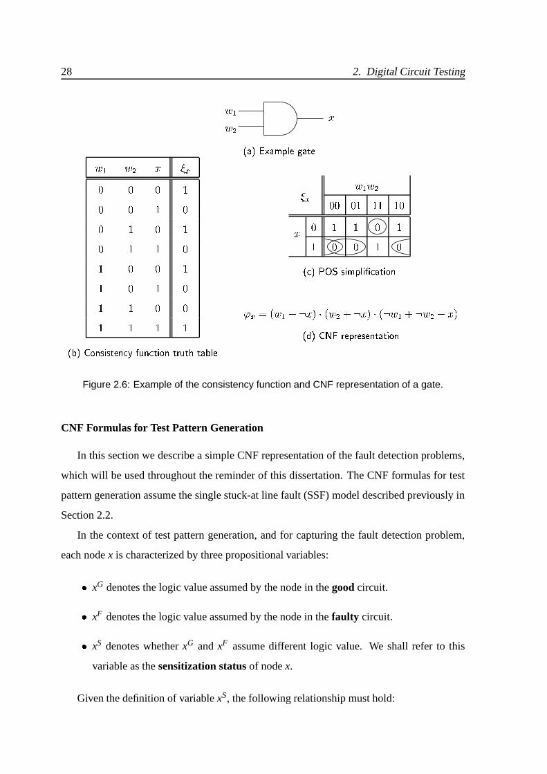
2.6 Example of the consistency function and CNF representation of a gate. . . . 28
2.7 Definition of the composite logic values and the D-calculus. . . . . . . . . 35
2.8 Justification on a NAND gate by the (a) D-algorithm and (b) 9-V algorithm. 36
2.9 Example of (a) static and (b) dynamic learning. . . . . . . . . . . . . . . . 39
3.1 Branch-and-bound example for problem (3.3). . . . . . . . . . . . . . . . . 59
3.2 Cutting plane example for problem (3.3). . . . . . . . . . . . . . . . . . . 61
3.3 SAT-based linear search algorithm. . . . . . . . . . . . . . . . . . . . . . . 70
3.4 Heuristic algorithmic to compute Dw. . . . . . . . . . . . . . . . . . . . . 71
3.5 Using bounding in the ILP algorithm. . . . . . . . . . . . . . . . . . . . . 72
3.6 SAT-based branch-and-bound algorithm. . . . . . . . . . . . . . . . . . . . 74
4.1 Global formula organization for detecting all faults. . . . . . . . . . . . . . 86
4.2 Proposed formula organization for detecting all faults. . . . . . . . . . . . . 94
4.3 Internal structure representation of an input multiplexer µIj. . . . . . . . . . 96
4.4 The internal structure of the miter circuit, λ j. . . . . . . . . . . . . . . . . 98
xi
5.1 Simple circuit for which we want to force output e 1. . . . . . . . . . . . 119
5.2 Abstract view of a generalized 2-inputs AND gate (UAND). . . . . . . . . 121
5.3 Example of unspecified assignments for a simple circuit. . . . . . . . . . . 123
5.4 Node variables for (a) good and (b) faulty circuit when w1 is stuck-at-1. . . 126
5.5 Minimum-size test pattern for which no propagation path exists. . . . . . . 131
5.6 MTP Block Diagram (dash processes/data are optional). . . . . . . . . . . . 133
6.1 Generic test pattern generator model [Chakrabarty 97]. . . . . . . . . . . . 143
6.2 Example of two a Linear Feed Back Register (LFSR). (a) “Exhaustive” and
(b) non-exhaustive test generators for any initial vector. . . . . . . . . . . . 144
6.3 (a) The C17 benchmark circuit. (b) A set of test vectors for C17. . . . . . . 146
6.4 Test pattern generators for the C17 circuit using: (a) 3 bits; (b) 2 bits with
inverted outputs [Chakrabarty 97, Chen 95]. . . . . . . . . . . . . . . . . . 147
6.5 Test sequences that show the use of Ci j, Ui j and Si j variables and the evo-
lution of the compatibility graph. . . . . . . . . . . . . . . . . . . . . . . . 155
7.1 Graph representation of completely specified test patterns. . . . . . . . . . 170
7.2 Graph representation of a incompletely specified test patterns. . . . . . . . 171
7.3 Block diagram of power reduction algorithm. . . . . . . . . . . . . . . . . 178
7.4 A 2-Opt move: (a) orginal tour and (b) resulting tour. . . . . . . . . . . . . 180
A.1 The C17 circuit with a test pattern for fault x11 stuck-at-0 that imposes
s-irrelevancy. . . . . . . . . . . . . . . . . . . . . . . . . . . . . . . . . . 202
A.2 The C17 circuit with a test pattern for fault x11 stuck-at-0 that imposes
j-irrelevancy. . . . . . . . . . . . . . . . . . . . . . . . . . . . . . . . . . 203
A.3 Minimum-size test pattern for which no justification path is needed. . . . . 205
xii

List of Tables
2.1 CNF formulas for simple gates. . . . . . . . . . . . . . . . . . . . . . . . . 29
2.2 Definition of the fault detection problem for the stem fault z stuck-a-v. . . . 31
2.3 Fault specific formula and fault detection requirements for fault x11 stuck-a-1. 32
3.1 CPU times on selected benchmarks. . . . . . . . . . . . . . . . . . . . . . 77
3.2 Computed upper bounds. . . . . . . . . . . . . . . . . . . . . . . . . . . . 78
4.1 Upper bounds on the ILP formulation for the C17 benchmark circuit. . . . . 89
4.2 ILP for the minimum test set problem. . . . . . . . . . . . . . . . . . . . . 91
4.3 Upper bounds using the new formulation model for the C17 benchmark circuit.100
4.4 Estimated ILP size for some benchmark circuits. . . . . . . . . . . . . . . 103
4.5 The proposed ILP model for the minimum test set problem. . . . . . . . . . 104
4.6 Covering table for a set of faults. . . . . . . . . . . . . . . . . . . . . . . . 108
4.7 Test set compaction results for the IWLS circuits. . . . . . . . . . . . . . . 110
4.8 Test set compaction results for the ISCAS’85 circuits. . . . . . . . . . . . . 111
5.1 Interpretation of the new variables modeling unspecified assignments. . . . 120
5.2 Truth table of a generalized AND (UAND) using the new variables. . . . . 120
5.3 Generalized CNF formulas for simple gates. . . . . . . . . . . . . . . . . . 124
5.4 Truth table for the sensitization status. . . . . . . . . . . . . . . . . . . . . 128
5.5 Definition of the fault detection problem for the stem fault z stuck-at-v. . . . 129
5.6 Experimental results for the IWLS benchmarks (allowing 1000 conflicts per
faults). . . . . . . . . . . . . . . . . . . . . . . . . . . . . . . . . . . . . . 135
xiii

5.7 Experimental results for the ISCAS’85 benchmarks (allowing 100 conflicts
per fault). . . . . . . . . . . . . . . . . . . . . . . . . . . . . . . . . . . . 136
5.8 Experimental results for some of the ISCAS’85 benchmarks (allowing 1000
conflicts per fault). . . . . . . . . . . . . . . . . . . . . . . . . . . . . . . 136
6.1 Definition of variables Ci j, Ui j and Si j. . . . . . . . . . . . . . . . . . . . 152
6.2 Experimental results for IWLS benchmarks. . . . . . . . . . . . . . . . . . 161
6.3 Experimental results for ISCAS’85 benchmarks. . . . . . . . . . . . . . . . 162
7.1 Hamming cost reduction and CPU times for the IWLS benchmark circuits. . 182
7.2 Power reduction results for the IWLS benchmarks with vectors generated by
ATALANTA. . . . . . . . . . . . . . . . . . . . . . . . . . . . . . . . . . . . 184
7.3 Power reduction results for the IWLS benchmarks with vectors generated by
MTP. . . . . . . . . . . . . . . . . . . . . . . . . . . . . . . . . . . . . . . 185
7.4 Power reduction results for the ISCAS’85 benchmarks. . . . . . . . . . . . 187
7.5 Power reduction results for the ISCAS’85 benchmarks with the restricted
2-Opt algorithm (500 links examined). . . . . . . . . . . . . . . . . . . . . 188
xiv

List of Acronyms
ATPG - Automatic Test Pattern Generation (see page 33 in Section 2.3).
BCP - Binary Cover Problem.
BDD - Binary Decision Diagrams.
BIST - Built-In Self-Test (see pages 141 and 142 in Sections 6.1 and 6.2, respectively).
CAD - Computer-Aided Design.
CMOS - Complementary Metal-Oxide Semiconductor.
CNF - Conjunctive Normal Form (see page 25 in Section 2.2).
CPU - Central Processing Unit.
CUT - Circuit Under Test (see page 142 in Section 6.2).
DD - Double Detection (see page 46 in Section 2.4).
DFT - Design for Testability.
DIMACS - Center for Discrete Mathematics and Theoretical Computer Science.
EDA - Electronic Design Automation.
EFP - Essential Fault Pruning (see page 46 in Section 2.4).
EFR - Essential Fault Reduction (see page 47 in Section 2.4).
FPGA - Field Programmable Gate Array.
FPM - Force Pair-Merging (see page 46 in Section 2.4).
FSM - Finite State Machine.
IC - Integrated Circuit.
xv

ILP - Integer Linear Programming (see pages 53 and 56 in Sections 3.1 and 3.2, respec-
tively).
INESC - Instituto de Engenharia de Sistemas e Computadores.
INLP - Integer Nonlinear Programming (see page 53 in Section 3.1).
ISCAS - International Symposium on Circuits and Systems.
IST - Instituto Superior Tecnico.
IWLS - International Workshop on Logical Synthesis.
LFSR - Linear Feedback Shift Register (see page 142 in Section 6.2).
LP - Linear Programming (see page 53 in Section 3.1).
MCT - Ministerio da Ciencia e Tecnologia.
MILP - Mixed-Integer Linear Programming (see page 53 in Section 3.1).
MOS - Metal-Oxide Semiconductor.
MTFTG - Multiple Target Fault Test Generation (see page 46 in Section 2.4).
NLP - Nonlinear Programming (see page 53 in Section 3.1).
ORA - Output Response Analyzer (see page 141 in Section 6.1).
POS - Product of Sums.
ROFS - Reverse Order Fault Simulation (see page 39 in Section 2.3.1).
ROM - Read Only Memory.
RTL - Register Transfer Level.
RVE - Redundant Vector Elimination (see page 47 in Section 2.4).
SAT - Propositional Satisfiability (see page 40 in Section 2.3.2).
xvi

SSF - Single Stuck-at Fault (see page 15 in Section 2.1).
TBO - Two-by-One (see page 46 in Section 2.4).
TPG - Test Pattern Generator (see page 141 in Section 6.1).
TSP - Traveling Salesperson Problem (see page 170 in Section 7.3.1).
USP - Unique Sensitization Point (see page 37 in Section 2.3.1).
VHDL - VHSIC Hardware Description Language.
VHSIC - Very High Speed Integrated Circuit.
VLSI - Very Large Scale Integration.
ZOILP - Zero-One Integer Linear Programming (see pages 53 and 62 in Sections 3.1
and 3.3, respectively).
xvii

xviii

Chapter 1
Introduction
Contents
1.1 Motivation and Objectives
1.2 Original Contributions
1.3 Thesis Organization
1

2 1. Introduction
1.1 Motivation and Objectives 3
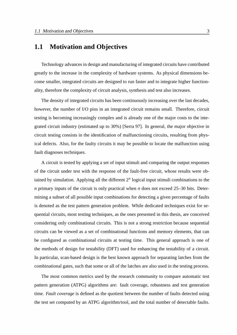
1.1 Motivation and Objectives
Technology advances in design and manufacturing of integrated circuits have contributed
greatly to the increase in the complexity of hardware systems. As physical dimensions be-
come smaller, integrated circuits are designed to run faster and to integrate higher function-
ality, therefore the complexity of circuit analysis, synthesis and test also increases.
The density of integrated circuits has been continuously increasing over the last decades,
however, the number of I/O pins in an integrated circuit remains small. Therefore, circuit
testing is becoming increasingly complex and is already one of the major costs to the inte-
grated circuit industry (estimated up to 30%) [Serra 97]. In general, the major objective in
circuit testing consists in the identification of malfunctioning circuits, resulting from phys-
ical defects. Also, for the faulty circuits it may be possible to locate the malfunction using
fault diagnoses techniques.
A circuit is tested by applying a set of input stimuli and comparing the output responses
of the circuit under test with the response of the fault-free circuit, whose results were ob-
tained by simulation. Applying all the different 2n logical input stimuli combinations to the
n primary inputs of the circuit is only practical when n does not exceed 25–30 bits. Deter-
mining a subset of all possible input combinations for detecting a given percentage of faults
is denoted as the test pattern generation problem. While dedicated techniques exist for se-
quential circuits, most testing techniques, as the ones presented in this thesis, are conceived
considering only combinational circuits. This is not a strong restriction because sequential
circuits can be viewed as a set of combinational functions and memory elements, that can
be configured as combinational circuits at testing time. This general approach is one of
the methods of design for testability (DFT) used for enhancing the testability of a circuit.
In particular, scan-based design is the best known approach for separating latches from the
combinational gates, such that some or all of the latches are also used in the testing process.
The most common metrics used by the research community to compare automatic test
pattern generation (ATPG) algorithms are: fault coverage, robustness and test generation
time. Fault coverage is defined as the quotient between the number of faults detected using
the test set computed by an ATPG algorithm/tool, and the total number of detectable faults.

4 1. Introduction
The goal of all ATPGs is to achieve 100% of fault coverage, i.e. to compute a test set that
detects all detectable faults in the circuit, for the selected fault model. Robustness refers to
the capability of the algorithm to identify all the non-detectable faults i.e. faults for which
no test pattern can be computed. Test generation time indicates how fast an ATPG algorithm
can compute a test set. Deterministic test generation is very complex, but ATPG algorithms
should be fast and the CPU time should scale well for large designs.
However, one might want to relax the test generation time constraint in favor of getting
an improved test set regarding some purposed metric, because the test pattern generation is
done once per design, but the testing of the circuit, using the computed test set, may be done
millions of times (in the production line and/or on the system). Therefore, the test generation
time may be not a key issue when the test set is generated with some optimization goal.
Besides the above metrics, that existing ATPG algorithms try to optimize, the field of
ATPG presents a large number of other challenging optimization problems of key signif-
icance that impact testing time, buit-in self-test (BIST), power dissipation, among others.
Unfortunately, the vast majority of these problems, when addressed, are most often solved
using heuristic approaches that do not guarantee an optimum solution.
The main objective of this thesis is to define formal optimization models for ATPG prob-
lems. We propose different models for problems concerning test set compaction, BIST, and
power dissipation. Moreover, for some of these problems we also present alternative heuris-
tic models/algorithms.
Discrete algorithms, in particular satisfiability search algorithms (SAT), for which test
pattern generation models exist, are also a promising technique for solving optimization
problems cast as integer linear programming (ILP) instances. An ILP instance is a mathe-
matical model to compute a set of integer values which optimize a given cost (or objective)
function subject to a set of linear constraints. Using a matrix notation a generic ILP problem

1.1 Motivation and Objectives 5
can be represented in the following general form:
minimize c xsubject to A x b (1.1)
and x
0
x is integer
where x is the vector of integer values to be determined, A is the matrix of constraints, and b
and c are generic vectors of coefficients. The discrete nature of this generic problem formu-
lation (1.1) makes it computationally hard. One approximated solution for these problems
can be computed by relaxing the restriction of x being integer, and then using well known
linear programming general methods (e.g. the Simplex algorithm). However, rounding the
computed real solution does not guarantee an optimal value of the cost function. This is
particularly significant in the case where the variables of the problem (the x vector) are con-
strained to binary values (0 or 1), i.e. we have a zero-one integer linear programming problem
(ZOILP).
Various techniques and algorithms exist for solving ILP problems. We study the use of
satisfiability algorithms for solving zero-one ILP1 problems using two different approaches:
the more well known linear search method [Barth 95], and a recent branch and bound method.
Implementations of both methods, based on the same SAT solver, and other generic, com-
mercial and academic, ILP solvers are evaluated. Given this evaluation we select the ade-
quate tool that will be used to solve the zero-one ILP optimization models proposed in the
remainder of the thesis.
The use of satisfiability algorithms also proved to be an effective approach for generic
ATPG. Satisfiability-based ATPG algorithms do not search the circuit structure directly to
identify a test pattern, as done by traditional algorithms like the D-algorithm [Roth 66], PO-
DEM [Goel 81] or FAN [Fujiwara 83]. Instead, satisfiability-based approaches construct an
algebraic formula that is subsequently used to compute the test pattern, by searching for one
1Sometimes, for a matter of simplicity we refer to generic ILP problems/models with the meaning of zero-
one ILP (ZOILP).
6 1. Introduction
of its solutions. Transforming the algebraic formula into a zero-one ILP problem is crucial
to establish formal optimization models for ATPG problems regarding some cost function.
However, these models are specific for each optimization test problem we are solving, and
must be tuned accordingly.
Determining the minimum number of test vectors that detect all detectable faults in a
circuit is a key issue in testing, because the size of the test set has a great impact on the
total testing time, especially in scan-based design testing. The size of the test has also great
influence on the resources needed to store the test patterns and the correct circuit outputs,
on the external testing machine or in the circuit itself. We propose a new exact model to
find the minimum test set for an arbitrary combinational circuit. The proposed ILP model
has a representation size that is polynomial in the size of the circuit description and which
is smaller than other existing solutions. Moreover, we describe several practical techniques
to further reduce the size of the proposed model. To determine the influence of different
strategies used by test pattern generators in the final test set size, a study is performed on test
set compaction obtained by using a set cover model over the generated test set.
The existence of unspecified inputs (or bits) in test patterns has several applications in
test optimization. However, the existing satisfiability-based test pattern generation models
use a logic of two values (0 and 1) where the don’t care value (X ) is not considered. There-
fore, in general, they are unable to compute test patterns which minimized the number of
specified inputs. We present a new model for test pattern generation for single stuck-at faults
in combinational circuits, where don’t cares are taken in consideration by using a logic of
three values (0, 1 and X ). The proposed solution is based on an ILP formulation which builds
on existing propositional satisfiability models for test pattern generation. The resulting ILP
formulation is linear on the size of the original SAT model for test generation, which is lin-
ear on the size of the circuit. The resulting algebraic formula is casted into a zero-one ILP
optimization model for computing test patterns with the maximum number of don’t cares,
i.e. the minimum number of specified inputs.
One important application of test generation with unspecified inputs is in BIST. The
main objectives of BIST are the design of test pattern generators circuits which achieve the
highest fault coverage, require the shortest sequence of test vectors and utilize the minimum

1.1 Motivation and Objectives 7
circuit area. Traditional BIST test generators are implemented with Linear Shift Feedback
Registers (LFSR) which generate pseudo-random sequences for the circuit under test. In
a simple BIST architecture the fault coverage depends on the testing time (i.e. number of
patterns in the sequence applied) and the initial seed of the pseudo-random generator (i.e. the
initial value of the LFSR). Many solutions have been proposed in order to reduce testing time
without reducing fault coverage, which, in general, result in some added circuitry causing an
area penalty. We propose a model to identify a minimal BIST test generator circuit, which
detects all detectable faults, assuming that some primary inputs can be declared equivalent
for testing purposes. The zero-one ILP model for test pattern generation with don’t cares is
then extended to identify compatibility relations between the primary inputs of the circuit
under test. The proposed model targets a specific built-in self-test architecture which is able
to reduce simultaneously the testing time and the test generator area overhead and still assure
100% fault coverage.
Other application of test set generation with a minimum number of specified inputs is
in the reduction of power dissipation during test set application. For a significant num-
ber of electronic systems used in safety-critical and/or mobile applications circuit testing is
performed periodically. For those systems, power dissipation during built-in self test can
represent a significant percentage of the overall power dissipation. One possible solution
to address this problem consists in reordering the test pattern sequence with the purpose of
reducing the amount of power dissipated during circuit testing. By reordering test pattern
sequences, one is able to reduce the circuit activity and consequently to minimize power
dissipation. Moreover, if the test patterns exhibit a large number of don’t cares the power
dissipated during test application can be further reduced because don’t cares can be spec-
ified with the appropriate logic value during test pattern sequence reordering. We propose
a zero-one ILP model for optimum pattern sequence reordering and don’t care assignment
that targets minimization of power dissipation during test set application. However, given the
complexity of the proposed model we also present an efficient heuristic-based approximation
algorithm, that reorders pattern sequences and assigns values to don’t care bits to minimize
the power dissipation during the test set application.
The work in this thesis was developed within the following research groups at INESC in

8 1. Introduction
Lisbon: ESDA – ELECTRONIC SYSTEM DESIGNS AND AUTOMATION group (http://esda.inesc.pt),
and SAT – SOFTWARE ALGORITHMS AND TOOLS FOR CONSTRAINT SOLVING group2
(http://sat.inesc.pt). Moreover, the present work was partially supported by two projects
from the Portuguese Ministry of Science and Technology (http://www.fct.mct.pt): GRASP
– Satisfiability algorithms for digital circuit analysis (PRAXIS 2/2.1/TIT/1597/95) and OPTI-
TEST – Models and algorithms for optimization problems in the digital system testing
(PRAXIS C/EEI/11266/98).
1.2 Original Contributions
The main original contributions in this thesis are: Development of a new formal model to compute the minimum size test set – To
our best knowledge, only two other approaches [Matsunaga 93, Silva 98] have pro-
posed non-heuristic solutions to the minimum test set problem for arbitrary combi-
national circuits. While the former has a worst-case exponential representation size,
the latter has a worst-case polynomial representation size, O n3 . The new model
has also a worst-case polynomial representation size, O n3 , but, for typical circuits
the size of the resulting ILP model is significantly smaller. For the selected bench-
mark circuits the size reduction can go up to 47% when comparing to the solution
in [Silva 98]. Extension of existing satisfiability-based ATPG models to compute test patterns
with don’t cares – Most satisfiability-based ATPG models use a two-value logic sys-
tem to map the circuit representation into an algebraic formula. Therefore, they can
not represent the existence of don’t care values in the circuit. These models have
been extended to use a three-value logic that efficiently supports don’t care represen-
tation. We developed the MTP ATPG tool by casting this model to an ILP problem
2The members of SAT group were part of the ALGOS – ALGORITHMS FOR OPTIMIZATION AND SIMU-
LATION group (http://algos.inesc.pt), until November 2000.

1.2 Original Contributions 9
that identifies, for a given fault, a test pattern with the minimum number of specified
inputs [Flores 98a, Flores 98b, Flores 98c]. Proposal of a new ATPG model targeting a minimal BIST circuit generator –
Most common BIST test patterns generators use LFSRs within some architectures
to reduce testing time without compromising fault coverage. [Chen 95] proposed a
counter-based test generator circuit with a reduced number of bits, that ensures 100%
fault coverage and requires less testing time, and smaller area, than traditional archi-
tectures. The number of bits in the counter depends on the number of primary inputs
that can be declared equivalent or compatible for testing purposes. We propose a new
ATPG model that computes test patterns maximizing the number of compatible in-
puts, thus minimizing the number of bits in the counter. This model was implemented
in the MTP-C ATPG tool [Flores 99b]. Development of new model for optimum test pattern reordering, and bit as-
signment targeting low-power testing – The minimization of the power dissipated
during testing became more important with the advent of mobile computation. Re-
ordering sequences of completely specified test patterns [Chakravarty 94] is a known
solution to reduce power dissipation during testing. However, the existence of don’t
cares in the test set can be used to further reduce power dissipation, but no model ex-
isted so far that supported it. We propose an ILP optimization model for assignment
and reordering of incompletely specified test sequences targeting minimum power
dissipation during testing. We also present heuristic algorithms for this problem and
show that the existence of don’t cares has a direct impact in the reduction of power
dissipation during testing [Flores 99a, Costa 98a, Costa 98b].
Other relevant contributions of this thesis are: Proposal of a optimization satisfiability-based algorithm – The use of satisfia-
bility algorithms to solve zero-one ILPs was proposed in [Barth 95]. However, the
algorithm described was shown to be particularly inefficient for a large number of
optimization instances [Silva 96a]. We propose the utilization and evaluate an algo-
rithm based on a branch and bound procedure, which is faster and solves more SAT
10 1. Introduction
based instances that other optimization tools (commercial and academic). The bsolo
algorithm was first described in [Manquinho 97]. Study of the effect of fault simulation in test set compaction – The use of set
covering algorithms for test set compaction was already proposed in [Hochbaum 96],
but only very preliminary experiments were conducted. We present a generic set
cover based compaction tool, MTSC, and study the impact of fault simulation in the
final test set size [Flores 99c].
1.3 Thesis Organization
This thesis is organized in 8 chapters which describe most of the research work devel-
oped. Each chapter was written to be, as much as possible, self-contained. Therefore some
subjects may be referred several times in different chapters.
After this introduction, we present in Chapter 2 some basic definitions used in the digital
circuit testing area and overview the most significant test pattern generator algorithms. We
group test pattern generation algorithms in two classes: structural or traditional algorithms,
that directly use the structure of the circuit to compute the test patterns; and satisfiability-
based algorithms, that use an algebraic formula generated from the circuit description, whose
solution, i.e. identifying a test pattern, is computed using “generic” satisfiability algorithms.
We give special attention to the generation of the algebraic formulas in Conjunctive Nor-
mal Formula (CNF) notation and describe in some detail existing propositional satisfiability
models for ATPG. We also describe heuristic techniques used during and/or after test pattern
generation to reduce the test set size, i.e. to obtain a compacted final test set.
In Chapter 3 we present an overview of the most common optimization models and algo-
rithms. We give particular emphasis to satisfiability-based algorithms for solving zero-one
ILPs and describe in some detail two approaches: linear search and branch and bound. We
evaluate several implementations of ILP solvers on different problems in order to select the
adequate solver for the instances that we will encounter in the remainder of the thesis.
In Chapter 4 we address the problem of determining the minimum size test set for a
circuit, a fundamental problem in digital system testing. However, unlike many competitive

1.3 Thesis Organization 11
solutions that have been proposed, which are based on heuristics, we focus our attention
on exact models. We describe a minimum test set reference model in which the size of the
zero-one ILP formulation is polynomial in the size of the circuit, O n3 . Then, we propose
a new model for minimum test set computation whose zero-one ILP formulation has, for
typical circuits, a representation size that is significantly smaller than previously existing
solutions. We present, for both models, some practical simplification techniques which are
able to significantly reduce the final size of the ILP formulation. However, as in the reference
model, the proposed model still grows cubically with the circuit size. Therefore, we consider
an alternative approach for computing a minimal test set size: we use a set covering model
to compact test sets that were obtained by an ATPG tool or any heuristic test set compaction
procedure. With this objective, recent and highly effective set covering algorithms are used
to compact the test sets of several benchmark circuits. We study the relationship between
the application of fault simulation and the ability of reducing the test set size and conclude
that by not using fault simulation and targeting all faults, we are able to compute a more
compacted test set.
In Chapter 5 we address the problem of test pattern generation for single stuck-at faults
in combinational circuits, under the additional constraint that the number of specified pri-
mary input assignments is minimized. We first extend the existing propositional satisfiability
model for test pattern generation to represent logic gates in which the don’t care value is
modeled. Then, we present the ILP formulation for computing test patterns with the mini-
mum number of specified inputs, whose size complexity is linear on the size of the circuit.
Some limitations of the proposed model are discussed in order to identify the conditions
when the optimum solution of the model does not correspond to the minimum unspecified
vector that detects a given fault. Results on benchmark circuits are presented which val-
idate the practical applicability of the test pattern minimization model and associated ILP
algorithm.
In Chapter 6 we derive a model for test generation with maximum width compression in
order to identify minimal BIST test generators. We present a brief overview of BIST circuit
generators and of the most used techniques to achieve high fault coverages with: short test-
ing times and minimum circuit area overhead. The notion of compatibility relations between

12 1. Introduction
primary inputs of the circuit under test is formally introduced. The proposed algorithmic
solution is based on an ILP formulation that builds on the previously proposed propositional
satisfiability model for test pattern generation with don’t cares. Extra constraints are intro-
duced to identify the maximum number of compatibility classes that determine which inputs
are equivalent for testing purposes. Due to a limitation of the available optimizer, we had to
relax the objective function of the model. Even though, we are able to illustrate the practical
applicability of our approach for a wide range of benchmark circuits.
In Chapter 7 we address the problem of power reduction during test set application.
We present the power dissipation model for generic CMOS circuits and use an estimation
model based on the Hamming distance, to evaluate the power dissipated by any test pattern
sequence. Hence, by reordering test pattern sequences we are able to minimize power dissi-
pation. This problem can be modeled as an instance of the traveling sales-person problem,
provided the test sequence does not exhibit don’t cares. For test sequences with don’t cares a
new ILP model is developed. The proposed model makes possible the identification of both
the optimum test pattern sequence and the values to be assigned to each don’t care bit in
order to minimize the total “power dissipation” during testing. Due to the complexity of the
proposed “exact” optimization model, we developed a heuristic-based algorithm for comput-
ing approximated solutions for this problem. We present results showing that the proposed
heuristics effectively reduce the power dissipated during the application of a test set, and
that the Hamming distance between consecutive test vectors has good correlation with the
computed power dissipation.
Finally in Chapter 8, we present the conclusions of this thesis and provide directions for
future research.
The three appendixes included at the end of the document contain two proofs and an
algorithm description that were removed from the main document to improve its readability:
(1) establish the accuracy of the model proposed in Chapter 5 to compute test patterns with
don’t cares; (2) prove that the set of constraints used in Chapter 7 eliminates all partial
sequences of test patterns without excluding any complete sequence and (3) describe the
Christofides algorithm used in Chapter 7 to define an initial solution for the test pattern
sequence.

Chapter 2
Digital Circuit Testing
Contents
2.1 Introduction
2.2 Basic Definitions
2.3 Automatic Test Pattern Generation
2.3.1 Structural/Traditional Algorithms
2.3.2 Satisfiability-Based Algorithms
2.4 Heuristic Test Set Compaction Algorithms
2.5 Conclusions
13

14 2. Digital Circuit Testing

2.1 Introduction 15
2.1 Introduction
Circuit testing can be performed at several abstraction levels: at the circuit level, at the
board level and at the system level. While testing at the latter two levels emphasizes fault
location for repair purposes, testing at the circuit level has, in most cases, a single purpose:
to distinguish between good and faulty circuits.
Faulty circuits occur when physical causes, called defects, change the layout of the cir-
cuit during fabrication. These defects are translated into electrical faults and, thereafter, are
translated into logical faults such that they can be tested with logical signals. This mapping
of defects into electrical, and thereafter into logical faults is called fault modeling. Various
fault models exist for digital circuits which consider not only permanent failures but also
temporary failures [Mourad 87, Abramovici 90]. The most common fault model assumes
single stuck-at faults (SSF) even though it is clear that this model does not accurately rep-
resent all actual physical defects. Moreover, as we will see, the advantages of the single
stuck-at fault model assures its usage in the most recent technologies [Aitken 99].
For a given fault model, the problem of test pattern generation consists of finding logical
input stimuli, which, in the presence of the targeted faults, will produce a response on circuit
outputs that differs from the expected response. The test generation process for different
fault models is computational hard, and it has already been proven to be NP-complete for
SSF [Fujiwara 82, Krishnamurthy 84]. The challenge of automated test pattern generation
(ATPG) consists of designing algorithms and heuristics which generate test sets in minimal
time but with a maximal fault coverage and with a minimal test set application time. This
latter goal is, in general, achieved by reducing (compact) the size (i.e. the number of vectors)
of the final test set.
In this chapter we introduce basic definitions used in the digital circuit testing area and
the major automatic test pattern generation algorithms along with some techniques to reduce
test set size. The chapter is organized in three main sections. In the first section we present
some basic test definitions, most of them based on [Abramovici 90]. We address the problem
of fault modeling concentrating our attention on the single stuck-at fault model. Using this
model we present the formal definition of fault detection and fault redundancy, and study

16 2. Digital Circuit Testing
the relation of faults that must be targeted to generate a complete test set. Since most of
the models proposed in this dissertation use the satisfiability framework, we describe, also
in this section, how an algebraic formula for test pattern generation is derived from a circuit
description.
In the second section, we describe the most popular ATPG algorithms. Chronologically,
we briefly discuss the techniques introduced by each algorithm to improve the overall perfor-
mance of test pattern generation. However, we distinguish two classes of ATPG algorithms,
structural algorithms, where the search process is directly based on the structure of the cir-
cuit, and satisfiability algorithms, where the search process is done over an algebraic formula
generated from the circuit description.
In the third section, we study some heuristic-based algorithms for test set compaction.
Most algorithms use a combination of methods that can be classified into compaction dur-
ing test generation or post-generation compaction [Chang 95], also referred to as dynamic
compaction or static compaction, respectively [Kajihara 95].
2.2 Basic Definitions
Fault modeling
Faults represent the effect, on the behavior of the modeled system, of physical defects
that occur during circuit manufacturing or during circuit operation. For systems described
at the logic level it is common to separate the logic function from the temporal attributes.
Therefore we also distinguish between logical faults that affect the logic function and delay
faults that affect the operating speed of the circuit. We will focus our attention in the former
category, the logical faults, because they are widely accepted in IC industry since they are
easier to test in production than the delay faults.
Fault modeling is closely related to the type of model/description used for the circuit.
Faults defined based on a structural description of the circuit are referred to as structural
faults; their effect is to modify the interconnection among components (e.g. gates, transistors,
etc). Faults defined using a functional model are denoted as functional faults; their effect is
to modify the behavior of functional blocks (e.g. changing a truth table of a component or

2.2 Basic Definitions 17
inhibit an RTL operation). For both types of faults we should be able to determine the output
of the circuit in the presence of the fault.
We assume that we have at most one logical fault in the circuit we are testing. However,
if multiple faults are present in the circuit we can still use the single-fault assumption for test
pattern generation, because, in most cases, a multiple fault can also be detected by the tests
generated for individual single faults that compose the multiple one. But, for those small
number of circuits in which fault masking occurs, i.e. the presence of multiple faults are not
detected by the test set, then a multiple stuck-at fault model should be used [Abramovici 90].
Structural faults consider only that two types of defects affect the interconnections be-
tween components: shorts and opens. A short results from the connection of two points
not intended to be connected, while an open results from the breaking of a connection. For
CMOS circuits, and other technologies, a short between an electrical node and the ground or
the power supply corresponds to fix that node to a predefined voltage level. From the logical
point of view this fault corresponds to have the signal of that node stuck at a fixed logic
value. These faults are denoted as stuck-at-0 or stuck-at-1, respectively. A short between
two signal lines usually creates a new logic function. This type of short represents a new
logical fault referred to as a bridging fault.
In many technologies, an open on a unidirectional signal line with only one fanout is
equivalent to assume that the line has a constant value. Therefore the line appears to be
stuck-at some logic value and the logical stuck-at fault model can be used. This model can
be also used if the line assumes a constant value resulting from a physical fault internal to
the component that drives the line. An open in a signal line with fanout may result in a fault
that is associated only with some fanout branches. To use the single-fault stuck-at model we
have to consider all the fanout branches faults separately and the stuck-at fault of the whole
line, the stem fault. Figure 2.1 shows a circuit with several physical defects that result in
two shorts (line d shorted to power and line f shorted to ground) and an open in line c (line
c was broken in two path, c and c ). The short defects are modeled by simple stuck-at-1
and stuck-at-0 faults, respectively. The open defect can be modeled by a stuck-at-0 fault in
the fanout branch c (assuming that we are using a technology in which dangling inputs are
interpret as logic level 0).

18 2. Digital Circuit Testing
i
a
b
cd
e
f
g
h
c’
stuck-at-1
stuck-at-0
stuck-at-0
Figure 2.1: Using the stuck-at fault model to model shorts and open defects.
There are other fault models. For example, we can assume that faults are located in the
transistors using the stuck-on fault model, in which a MOS transistor is always on, or stuck-
open fault model, in which a transistor in the pull-up or pull-down path is open introducing
some memory in the circuit [Mourad 87]. Fault models like this are more realistic because
they model more closely the actual physical defects. However, in practice the simple stuck-at
fault model has been found to work well and we concentrate on this model [Abramovici 90,
Smith 97].
The single stuck fault model is also denoted as classical or standard model because it
was the first model and it has been widely studied and used. Despite being known that the
model validity is limited, the single stuck model has a set of attributes that makes its usage
very attractive [Abramovici 90]: As we noted, it may represent different physical defects. The model is independent of the technology. Since the model deals only with inter-

2.2 Basic Definitions 19
connection lines being stuck-at a given logic value, it can be used for the implemen-
tation of the circuit in different technologies. Experience has shown that the test vectors used to detect single stuck-at faults in
general detect many other non-classical faults. The number of single stuck-at faults is small compared to the number of faults in
other fault models. Moreover, as we will show, the number of faults considered for
test pattern generation can be reduced by fault collapsing techniques. The single stuck fault model can be used to model other types of faults by introducing
“virtual logic” in the circuit that changes the behavior of some lines [Abramovici 90].
Fault Detection and Redundancy
Let us consider a circuit C that implements a combinational logic function denoted as
gC x , where x represents the input vector. We refer to a test vector (or test pattern) as a input
vector (primary input assignments) with the main purpose of detecting the existence a given
fault or faults in the circuit.
Definition 2.1 (Test pattern) We define a test pattern (or test vector) t as an assignment to
the primary inputs, such that some assignments may be unspecified, i.e. t x1 v1 xn vn
for all xi PI and with vi 0 1 X .Definition 2.2 (Test pattern specification) A test pattern t is completely specified when-
ever t x1 v1 xn vn
for all xi PI and with vi 0 1 . Otherwise, t is said to be
incompletely specified.
The output response of the circuit to a test vector t is denoted as gC t . Note that, if the
circuit has multiple outputs the resulting output gC t is a vector. The existence of fault f
in the circuit modifies its functionality and a new combinational function is defined by the
circuit, g fC x . Note that we are only considering faults that do not change the combinational
characteristic of the circuit (i.e. faults that do not introduce memory and sequential behavior).

20 2. Digital Circuit Testing
Definition 2.3 (Fault detection) A test vector t detects a fault f if and only if t distinguishes
the outputs from the good and faulty circuit:
gC t g fC t
A circuit is tested by applying a test sequence t1 t2 tm denoted as test set T . For
a combinational circuit this sequence of vectors can be applied in any order and if any test
vector reveals the existence of a fault then the circuit is marked as defective and the test can
stop.
A test vector detects a stuck-at-v fault f if two conditions are satisfied:
1. The test vector activates the fault f , i.e. distinguishes the good and the faulty circuits
by forcing the site of the fault to assume the opposite value of v.
2. The test vector propagates the error to a primary output, i.e. there is at least one path
between the fault site and a primary output for which the lines on the good and the
faulty circuits along that path, assume opposite values1.
Definition 2.4 (Sensitized path) A line whose value for test vector t changes in the presence
of a fault f is said to be sensitized to fault f by test t. A path composed of sensitized lines is
called a sensitized path.
In a circuit with a gate whose output is sensitized has at least one input sensitized, with
the obvious exception of the fault site. Moreover, all other inputs of that gate that are not
sensitized must assume a the non-controlling value (nc) of the gate, i.e. the logic value that
forces the gate to go into transparent mode (when the output follows the input), if such value
exists. For example, in a 2-input AND gate if the output is sensitized then one input must
also be sensitized and the other input must assume the logic value 1, the non-controlling
value of an AND gate.
Definition 2.5 (Detectable/undetectable fault) A fault f is said to be detectable if exists a
test t that detects f . If such a test vector does not exist then the fault f is an undetectable
fault (also referred as redundant fault).
1Sometimes it is used the term “fault propagation” with the meaning of “error propagation” or “fault effect
propagation”.

2.2 Basic Definitions 21
A circuit in a presence of an undetectable fault f does not alter its logical function,
therefore g fC x gC x and no test exists that can simultaneous activate f and create a
sensitized path to a primary input.
In general, a test set that is able to detect all detectable faults in the circuit is referred to as
a complete test set. However, the existence of undetectable faults may prevent a test set to
detect some detectable faults because, an undetectable fault may masquerade the erroneous
behavior of a detectable fault [Abramovici 90].
Definition 2.6 (Redundant/irredundant circuit) A combinational circuit that contains un-
detectable stuck-at faults is said to be redundant. A combinational circuit in which all stuck-
at faults are detectable is said to be irredundant.
A redundant circuit can always be simplified by removing at least one gate or gate input.
For example, if the undetectable fault is a stuck-at-0 on an input of an AND gate then the
gate could be removed and its output line connected to logic level 0. Note that, because the
fault is redundant, its existence does not change the behavior of the circuit therefore, we can
assume that the fault site is always connected to logic 0, in this case, and then simplify the
logic. Observe, however, that redundancy can be useful for reducing circuit delay or to avoid
circuit hazards [Keutzer 90, Abramovici 90].
Test pattern generation for large combinational circuits is computationally hard. In gen-
eral, most test pattern generators stop test generation for a target fault when the process
becomes too costly (in terms of time, memory, etc). Therefore the resulting test set may not
be a complete one, because some detectable faults are not detected. Consequently, it is usual
to distinguish between undetectable faults and faults that are detectable but for which no
vector could be computed during test pattern generation for the available CPU time and/or
memory resources.
Definition 2.7 (Aborted fault) A non-redundant fault for which no vector is computed dur-
ing test pattern generation, due to computational resource limitations, is referred to as an
aborted fault.
The existence of aborted faults in a test set conditions the effectiveness, or quality, of the
test set. Quality test evaluation is done in the context of a fault model, e.g. stuck-at fault

22 2. Digital Circuit Testing
model, and is related with the total number of detectable faults identified by the model and
the effective number of faults detected by the test set.
Definition 2.8 (Fault coverage) For a given fault model, the ratio between the number of
faults detected by a test set and the total number of faults in the assumed fault universe is
referred as fault coverage [Abramovici 90].
The fault universe is composed only of detectable faults, and excludes the redundant
faults which should be identified by the test pattern generator algorithm. In some cases,
the final test set quality is evaluated via fault simulation, where the circuit is simulated to
determine/confirm the faults that are effectively detected.
Fault Equivalence and Dominance
The number of single stuck-at faults in a combinational circuit with n signal lines is 2 n,
where the value of n is calculated considering that every fanout branch is a distinct signal
line. The number of faults to be considered for test pattern generation can be reduced by
grouping faults according to their effect on the circuit.
Definition 2.9 (Equivalent faults) Two faults f and f are equivalent in a circuit C if and
only if g fC x g f
C x .Since the combinational function of a circuit is the same in the presence of each equiv-
alent fault, then the equivalent faults are detected by the same set of test patterns. All the
single stuck-at faults of a circuit can be grouped into equivalence classes where all the faults
are equivalent among themselves. For test set computation we need only to consider one
representative fault from each equivalence class. Figure 2.2 shows an example of equivalent
fault collapsing for a 2-input NAND and OR gate. In general for a simple n-input gate with
a controlling value we need only to consider n 2 single stuck-at faults: one stuck-at-0 and
one stuck-at-1 on the output and one stuck-at to the non-controlling value of the gate in each
input.
The number of faults that must be considered to compute a complete test set can be
further reduced using another fault relation.

2.2 Basic Definitions 23
PSfrag replacements
a
bc
x
yz
stuck-at-0 fault
stuck-at-1 fault(a) (b)
Figure 2.2: (a) NAND and OR gates with uncollapsed fault set. (b) Equivalence fault col-
lapsing.
Definition 2.10 (Dominating fault) A fault f is said to dominate another fault f if all the
tests that detect f include all the tests for detecting f .If Tf and Tf are the sets of all test patterns that detect faults f and f , respectively, then
fault f dominates f provided Tf Tf . Therefore, it is only necessary to compute a test
pattern for f because the same pattern will also detect the dominating fault f .
In general, fanout stem stuck-at faults dominate fanout branches faults and, in simple
gates with a controlling value c and an inversion i, the output stuck-at- c i fault dominates
any input stuck-at-c fault. In these cases the stem stuck-at faults and output faults can be
removed from the set of faults we consider for test generation. The reduction of the set of
faults using the dominance relation is called dominance fault collapsing.
Using both equivalence fault collapsing and dominance fault collapsing, we can reduce
the target fault set of a circuit to a minimum that is sufficient to compute a complete test set.
Figure 2.3 shows a simple circuit where the number of target faults is reduced form 14 faults
to 6 faults using the two collapsing techniques.
Combinational Circuits Definitions
We start by introducing a unified representation for combinational circuits that will be
used throughout the dissertation. A combinational circuit C with N nodes is represented as

24 2. Digital Circuit Testing
PSfrag replacementsaa
bbcc
yyzz
stuck-at-0 fault
stuck-at-1 fault
Figure 2.3: Using fault equivalence and fault dominance to collapsed the fault set to a mini-
mum.
a directed acyclic graph C VC EC , where the elements of VC, i.e. the circuit nodes, are
either primary inputs or gate outputs, and with VC ! N. The set of edges EC VC " VC
identifies gate input-output connections. We shall assume gates with bounded fanin, and so EC # O $ N . For every circuit node x in VC, the following definitions apply: O x denotes the fanout nodes of node x, i.e. nodes y in VC such that x y EC. O %! x denotes the transitive fanout of node x, i.e. the set of all nodes y such that
there is a path connecting x to y. I x denotes the fanin nodes of node x, i.e. nodes y in VC such that y x EC. I %& x denotes the transitive fanin of node x, i.e. the set of all nodes y such that there
is a path connecting y to x. KO x denotes immediate fanout cone of influence of x, being defined as follows:
KO x y y O % x (' y I w () w O % x (2.1)
KI x denotes immediate fanin cone of influence of x, being defined as follows:

2.2 Basic Definitions 25
KI x *+-,y . O /10 x 2 I % y 43576 O % x 98 x (2.2)
The set of primary inputs can also be referred to as PI, and the set of primary outputs
as PO. Simple gates are assumed: AND, NAND, OR, NOR, NOT and BUFF. Finally, the
number of stuck-at faults in the circuit is M, with M O N , since we assume EC O $ N ,and are numbered 1 M. The example in Figure 2.4 illustrates the previous definitions for
the ISCAS’85 [Brglez 85] benchmark circuit C17.
Conjunctive Normal Form Formulas
The representation of the circuit function can be described using any type of Boolean
functions or formulas. However, we will use the conjunctive normal form (CNF) formulas
because they are easily manipulated programmatically [Larrabee 92]. A CNF formula ϕ
on n binary variables x1 xn is the conjunction (AND) of m clauses ω1 ωm each of
which is the disjunction (OR) of one or more literals, and where a literal is the occurrence
of a variable xi or its complement : xi. A formula ϕ denotes a unique n-variable Boolean
function f x1 xn and each of its clauses corresponds to an implicate of f . Figure 2.5
shows a CNF formula that contains 3 clauses and 7 literals using 3 variables (x y and z).
An assignment for a formula ϕ is a set of variables and their corresponding Boolean values,
represented as variable/value pairs; for example A x1 0 x7 1 x13 0 which can also
be denoted as A x1 0 x7 1 x13 0 . The value assumed by a formula ϕ given
an assignment A is denoted by ϕ A and can yield three possible outcomes: ϕ A 1 and we say
that ϕ is satisfied and A is referred to as an satisfying assignment; ϕ A 0 in which case ϕ is
unsatisfied and A is referred to as an unsatisfying assignment; and ϕ A X indicating that the
value of ϕ cannot be resolved by the assignment A. The last case can only happen when A
is a partial assignment, i.e. not all variables are involved in the assignment. For example, the
assignment A x 1 y 1 to the formula of Figure 2.5 will result in ϕ X because
the value for the third clause can not be determined, it is an unresolved clause.
The CNF formula of a gate denotes the consistent input-output assignments to the gate.

26 2. Digital Circuit Testing
x16
x10x1
x3
x6
x7
x2
x19
x22
x23
x11
(a)
;=<>=?@A
B=CDFE
G=HJIK=LJLMNPO
QRPSTUPV
WX!Y
Z[\[ Node x x11
O x x16 x19 O %! x x16 x19 x22 x23 I x x3 x6 I % x x3 x6 KO x x2 x7 x10 x16 x19 x22 x23 KI x x10 x2 x7 x1 x3 x6
(c)
Figure 2.4: (a) Example circuit, C17, (b) graph representation (c) and topological data for
node x11.

2.2 Basic Definitions 27
]_^`badcfehgji(`lknmocpehgji(`Pkqarcfmocsktehguwvyxz|h~
#h #Figure 2.5: An CNF formula with 3 clauses and 7 literals.
Therefore, the CNF formula of a circuit is the conjunction of the CNF formulas for each
gate output, because each individual gate have to have consistent assignments in its inputs-
output. Figure 2.6 shows the consistency function, ξx, for a 2-input AND gate, which models
the consistent assignments on the gate inputs and output. Figure 2.6 also shows the resulting
CNF formula of the AND gate obtained as the product of sums (POS) representation of ξx.
For a j-input AND gate, x AND w1 w j the resulting CNF formula is [Larrabee 92,
Stephan 96, Silva 97b],
ϕx j
∏i 1
wi _: x 4 j
∑i 1
: wi x (2.3)
A complete list of the CNF formulas for simple gates with an arbitrary number of inputs
is reproduced in Table 2.1 [Silva 97b]. If we view a CNF formula as a set of clauses, the
CNF formula for the circuit is defined by the set union of the CNF formulas for each gate
with output x, ϕx:
ϕ ,x . VC
ϕx (2.4)
Given the CNF formula ϕ for a circuit and an assignment API to the primary inputs, then
the assignment AC denotes the values on the circuit nodes obtained from API by implying the
assignments on all gate outputs [Abramovici 90].
28 2. Digital Circuit Testing
¡ ¡ ¡ ¡ ¡ ¡ ¡ ¡¡ ¡ ¡ ¡ ¡ ¡ ¡ ¡¢4£¥¤¦¨§ª©$«¬ «44®©#¯°±4²&©#¯¬ §y©³´w²$µ³4¶£!· ®
¸³¹º» ¼½b¾À¿ÂÁ&ÃÀ¾!ÄÅ!Æ ÇÉÈ&¾$Ê4Ç
ËwÌ$ÍΨÏÑÐ|ÒÓÕÔÖ!×ØÓ ÙyÌ\Ú$ÛÓ ÜyÝÞ#ß à³áàâãªã ãåä äªä äÀãæ ã ä ä ã ää ã ã ä ã
çéèëêíìbî³ïjðòñtóôöõ÷ìbîøtðsñqóôqõ(ìPñtî³ïjðòñöîøtðùóôúwûªüýÿþ Figure 2.6: Example of the consistency function and CNF representation of a gate.
CNF Formulas for Test Pattern Generation
In this section we describe a simple CNF representation of the fault detection problems,
which will be used throughout the reminder of this dissertation. The CNF formulas for test
pattern generation assume the single stuck-at line fault (SSF) model described previously in
Section 2.2.
In the context of test pattern generation, and for capturing the fault detection problem,
each node x is characterized by three propositional variables: xG denotes the logic value assumed by the node in the good circuit. xF denotes the logic value assumed by the node in the faulty circuit. xS denotes whether xG and xF assume different logic value. We shall refer to this
variable as the sensitization status of node x.
Given the definition of variable xS, the following relationship must hold:

2.2 Basic Definitions 29
Gate type Gate function ϕx
AND x AND w1 w j j
∏i 1
wi _: x j
∑i 1
: wi x NAND x NAND w1 w j
j
∏i 1
wi x j
∑i 1
: wi _: x OR x OR w1 w j
j
∏i 1
4: wi x j
∑i 1
wi _: x NOR x NOR w1 w j
j
∏i 1
4: wi _: x j
∑i 1
wi x NOT x NOR w1
x w1 4: x _: w1
BUFFER x BUFFER w1
4: x w1 x _: w1
Table 2.1: CNF formulas for simple gates.
xG xF xS xG : xF xS 4: xG xF xS (2.5) xG xF _: xS 4: xG _: xF _: xS
which basically states that the logic values of xG and xF differ if and only if xS assumes logic
value 1.
Let ϕx denote the CNF formula associated with gate output x. The notation ϕGx denotes
the CNF formula for x in the good circuit, i.e. using xG variables, whereas ϕFx denotes the
CNF formula for x in the faulty circuit, i.e. using xF variables. For a stem fault z stuck-a-

30 2. Digital Circuit Testing
v, the CNF representation of the associated fault detection problem contains the following
components: CNF formula denoting the good circuit, ϕG. CNF formula denoting the faulty circuit, ϕF . This formula only needs to contain the
CNF formulas for the nodes that are relevant for detecting the given fault, i.e. nodes
in the transitive fanout of node z. CNF formulas for defining the sensitization status of every node in the transitive
fanout of the fault site, i.e. node z. Hence, for each of these nodes, ϕSx , is given
by (2.5) which requires xS 1 if and only if xG xF . Clauses requiring xG xF on each node x such that x is not in the transitive fanout of
z but at least one fanout node of x is in the transitive fanout of z, i.e. x is in KO z F6O % z . Observe that this condition permits restricting the number of clauses and the
number of xF and xS variables that must actually be used. Clauses capturing conditions for activating the fault on node z, i.e. by requiring zG zF and by forcing a suitable logic value on zG. Finally, we guarantee that the fault effect is observed at a primary output by requiring
that for at least one primary output x, xS 1.
The formula for detecting a fault z stuck-a-v is summarized in Table 2.2 and will hence-
forth be referred to as the fault detection formula, ϕD. Similarly, we defined the fault
specific formula, ϕFS , as follows,
ϕFS ϕD 6 ϕG 8 ϕR ϕF 8 ϕS 8 ϕE 8 ϕA (2.6)
which contains only the clauses associated with the propagation of the error signal to the
primary inputs. The fault specific CNF formula for fault x11 stuck-a-1 on the example circuit
C17 (see page 26) is given in Table 2.3.

2.2 Basic Definitions 31
Sub-formula/Condition Clause Set
Good Circuit ϕG ,x . VC
ϕGx
Faulty Circuit ϕF ,x . O /0 z 2 ϕF
x
Node Sensitization ϕS ,x . O / 0 z 2 ϕS
x
Side Input Equivalence ϕE 4: xG xF ¥ xG : xF x KO z ¨6 O % z Fault Activation Conditions ϕA ! zS 4: zG zF if v 1
zS zG 4: zF if v 0
Fault Detection Requirement ϕR ∑x . PO " x . O / 0 z 2 xS
Detection of Fault z stuck-a-v ϕD ϕG 8 ϕF 8 ϕS 8 ϕE 8 ϕA 8 ϕR
Table 2.2: Definition of the fault detection problem for the stem fault z stuck-a-v.
The CNF formula for fanout-branch faults requires additional information for dealing
with setting specific values on the fanout branch. For a given fanout branch fault z y stuck-
a-v 2, the CNF formula of Table 2.2 needs to be modified as follows:
2The fanout branch from node z to y is denoted by edge # z $ y % that in ISCAS’85 notation is represented as
z &(' y.

32 2. Digital Circuit Testing
Sub-formula/Condition Clause Set
Fault Circuit ϕF *) ϕFx168 ϕF
x198 ϕF
x228 ϕF
x23 +Node Sensitization ϕS -, ϕS
x168 ϕS
x198 ϕS
x228 ϕS
x23 .Side Input Equivalence
ϕE P: xG2 xF
2 xG
2 _: xF2 P: xG
7 xF7 xG
7 _: xF7 P: xG
10 xF10 ¥ xG
10 _: xF10
Fault Activation Conditions ϕA xS11 ¥4: xG
11 xF
11
Fault Detection Requirement ϕR xS22 xS
23
Table 2.3: Fault specific formula and fault detection requirements for fault x11 stuck-a-1.
For all sub-formulas in Table 2.2, replace node z by node y. Replace the fault activation formula ϕA as follows:
– Add a clause requiring yG yF which causes the creation of the fault effect:
yG yF yG yF : yG : yF (2.7)
– Require zG 1 or zG 0 depending on whether the fault is stuck at 0 or 1,
respectively. If the gate with output y has a non-controlling value [Abramovici 90], nc y , require
that the side inputs of y with respect to z to assume the non-controlling value of y,
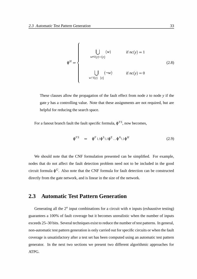
2.3 Automatic Test Pattern Generation 33
ϕH !
,w . I 0 y 20/21 z 3 w if nc y 1,
w . I 0 y 20/41 z 3 P: w if nc y 0
(2.8)
These clauses allow the propagation of the fault effect from node z to node y if the
gate y has a controlling value. Note that these assignments are not required, but are
helpful for reducing the search space.
For a fanout branch fault the fault specific formula, ϕFS, now becomes,
ϕFS ϕF 8 ϕS 8 ϕE 8 ϕA 8 ϕH (2.9)
We should note that the CNF formulation presented can be simplified. For example,
nodes that do not affect the fault detection problem need not to be included in the good
circuit formula ϕG. Also note that the CNF formula for fault detection can be constructed
directly from the gate network, and is linear in the size of the network.
2.3 Automatic Test Pattern Generation
Generating all the 2n input combinations for a circuit with n inputs (exhaustive testing)
guarantees a 100% of fault coverage but it becomes unrealistic when the number of inputs
exceeds 25–30 bits. Several techniques exist to reduce the number of test patterns. In general,
non-automatic test pattern generation is only carried out for specific circuits or when the fault
coverage is unsatisfactory after a test set has been computed using an automatic test pattern
generator. In the next two sections we present two different algorithmic approaches for
ATPG.

34 2. Digital Circuit Testing
2.3.1 Structural/Traditional Algorithms
Structural algorithms for ATPG are implemented using information from the structural
model of the circuit, and therefore, they are often characterized as topological. We also
denote this type of ATPGs as traditional because they were the first to appear, and because
they are extensively studied, documented and still used in many tools.
We will focus our attention only on algorithms that generate a test set for a specific target
fault, i.e. fault-oriented algorithms, as opposed to fault-independent algorithms whose goal
is to derive a test set which detects a large number of faults without targeting any individual
fault [Abramovici 90].
Most of the structural algorithmic solution for ATPG are based on the D-calculus [Roth 66]
or on its algebraic variations [Akers 78, Cha 78]. The D-calculus represents the value of a
line considering the logic value v, on the correct circuit (or good circuit), and the logic value
v f , on the faulty circuit. The composite logic value v 5 v f represents an error when v and v f
assume opposite logic values, v 5 v f 1 5 0 or v 5 v f 0 5 1 and are denoted as D and D, re-
spectively. The lines where v and v f assume the same logic value, v 5 v f 0 5 0 or v 5 v f 1 5 1
are denoted as 0 and 1, meaning that they are not affected by the presence of the fault f in
the circuit. The D-calculus has been shown to be a suitable framework for the fault detection
problem. A test pattern t detects a stuck-at fault f if at least one circuit output assumes the
value D or D under the D-calculus. The algebraic definition of the D-calculus is given in
Figure 2.7 where the X value denotes an unspecified composite value.
The D-algorithm [Roth 66] was the first algorithm to use the D-calculus for test patterns
generation. It starts by assigning the error D (D) to the faulty line that is stuck-at-0 (stuck-
at-1) and then proceeds with two objectives: propagate any error value, D or D, to a circuit output, so that the fault effect is ob-
servable; justify the internal line assignments, including the error value at the faulty line, by
identifying consistent assignments to the circuit primary inputs. The justification pro-
cess identifies consistent input assignments for each gate that has an assigned value
on the output but which is not implied by the current input values.

2.3 Automatic Test Pattern Generation 35
v 5 v f 0/0 1/1 1/0 0/1
Composite logic value 0 1 D D
NOT Out AND 0 1 D D X OR 0 1 D D X
0 1 0 0 0 0 0 0 0 0 1 D D X
1 0 1 0 1 D D X 1 1 1 1 1 1
D D D 0 D D 0 X D D 1 D 1 X
D D D 0 D 0 D X D D 1 1 D X
X X X 0 X X X X X X 1 X X X
Figure 2.7: Definition of the composite logic values and the D-calculus.
These objectives are achieved implementing a decision procedure that assign values to
the gates in one of the two frontiers:
D-frontier: consists of all the gates whose current output value is X but have one or more
error values (D or D) on their input lines.
J-frontier: consists of all gates whose output value is known but it is not implied (or
justified) by its current input values.
Therefore, at each decision step the D-frontier represents the gates which can be selected
to create one or more sensitized paths to one or more primary outputs, and the J-frontier
represents the gates whose inputs need to be justified. For some practical circuits, the orga-
nization of the D-algorithm may lead to large decisions trees, since a large number of internal
lines may be involved in the decision process.
The 9-V [Cha 78] algorithm is similar to the D-algorithm but uses a logic of nine val-
ues [Muth 76]. These nine values result from the combinations assignment of three logic
values 0 1 X to v 5 v f which results in four new partially specified composite logic values.
Using these new composite logic values the propagation of the error through multiple paths
is considered also during gate justification. For example, Figure 2.8 shows an NAND gate
sensitized with a single D input value and a D output value. While in the D-algorithm the

36 2. Digital Circuit Testing
687:9 ;=<?>
@ ABDCFE
GDHIGKJ-G LDMONQPSRTFUWVYXOZ\[^]_8`ab:cdegf a`h:iXOa`\]^j
k lmKnoOprq^s^t8u\vwgxyzg vu|:oOvu\s^~
Figure 2.8: Justification on a NAND gate by the (a) D-algorithm and (b) 9-V algorithm.
other input of this gate is set to 1 during justification, in the 9-V algorithm the input is set to
1 5 x. This assignment serve to justify “simultaneously” the logic value 1 or the error value
D, allowing in this situation a multiple path sensitization. Therefore, the flexibility provided
by the new composite logic values allows reducing the amount of search done for multiple
path sensitization. In a situation where k paths exist for error propagation, the D-algorithm
may eventually try all 2k 6 1 possible combinations while the 9-V algorithm will enumerate
at most k paths. However the advantages of using the 9-V algorithm are limited because
multiple path sensitization are rare in practical circuits [Cha 78].
PODEM (Path-Oriented Decision Making) [Goel 81] was the first ATPG algorithm that
restricted the search process to the primary inputs. This direct implicit enumeration of the
circuit inputs was shown an efficient technique to reduce the complexity of the D-algorithm.
Each step of the algorithm identifies an assignment objective, based on the D-frontier, and
maps it into the primary inputs by a simple backtrace procedure. This procedure identifies
each primary input, not yet assigned, that will contribute to satisfy the objective by “back-
ward justifying” at most one unspecified line per gate until a primary input is reached with
a logic value. Finally, this value on the primary input is propagated through the circuit.
This whole process continues until an error signal propagates to a primary output. The main
advantages of the PODEM algorithm over the D-algorithm are: inexistence of justification conflicts, since all values are assigned by forward impli-
cations;

2.3 Automatic Test Pattern Generation 37 no need to maintain a J-frontier, since there is no need for justification; no backward implication process, because all values are propagated forward; no backtrack procedure is required to manipulate the D-frontier and J-frontier and
restore a previous state; any change in the state is easily computed by propagating the
new values from the primary inputs (as also shown in [Snethen 77]).
The FAN (FAN-out-oriented test generation) algorithm [Fujiwara 83] has several im-
provements with respect to PODEM by changing the backtracing strategy in two distinct
ways. First, the backtrace procedure of FAN may stop at specific internal lines rather than
have to reach a primary input. These lines, denoted as head lines, are statically identified
as the outputs of fanout-free subcircuits. Observe that, the justification of the head lines
cannot cause conflicts and therefore is postponed to a final stage. Second, FAN uses a
multiple-backtrace procedure which attempts to satisfy a set of objectives simultaneously
rather than one objective at a time. For some set of objectives a multiple-backtrace proce-
dure can detect conflicting assignments, in particular, in fanout branches lines. Stopping
the multiple-backtrace procedure immediately and assigning the most requested value to the
fanout branches line avoids fruitless computation and leads to the early detection of incon-
sistency which would decrease the number of backtracks. FAN also introduced the notion
of unique sensitization points (USPs), unique lines that should always be sensitized for the
propagation of an error to a primary output. Upon the identification of USPs, which in FAN
occurs when the associated D-frontier has only one gate, the algorithm immediately gener-
ates all the necessary assignments to propagate the error on the identified lines. Since FAN
assigns values also to internal lines, the authors have implemented a backward implication
procedure that justifies those assignments as much as possible in order to improve the over-
all performance of the algorithm. The lines left unjustified after backward implication are
marked as the next set of objectives for justification using the multiple-backtrace procedure.
The ATALANTA [Lee 93] is an example ATPG tool that implements the FAN algorithm and
which will be extensively used in this dissertation.
TOPS (TOPological Search) [Kirkland 87] and SOCRATES [Schulz 88, Schulz 89] rep-
resent evolutions of FAN. The TOPS algorithm extended the concept of head lines of FAN to

38 2. Digital Circuit Testing
include sub-circuits that might have fanout, but all such fanout must completely re-converge
before the lines where the backtrace procedure stops. These lines, denoted as basis-nodes,
are also justified in the final stage of the algorithm, as the head lines are, even though such
justification may require some backtracking. TOPS formalized the notion of unique sensiti-
zation points (USPs), denoted as absolute dominators, and proposed processing algorithms
for their identification. The algorithms to identify either the basis-nodes or the absolute
dominators are based on graph analysis and use set operations (union and intersection), thus
having time complexity O N2 . TOPS also extended the PODEM algorithm to use nine
composite values [Muth 76] instead of five values. The SOCRATES algorithm uses the
same techniques of TOPS but using the “traditional” five logic values. The new concepts
introduced by SOCRATES were the static [Schulz 88] and dynamic learning [Schulz 89].
The learning process consists in the identification of global implications (sometimes also
referred as non-local implications) by assigning temporary logic values to “arbitrary” lines
in the circuit with the objective of examining their logical consequences. The static learn-
ing procedure is performed in a pre-processing stage based on the following logical identity
called contrapositive:
i f i vi j v j
then j v j i vi
(2.10)
where vi is the logical value assigned to line i and v j is the value assigned to line j by a impli-
cation procedure. A learning criterion is used to identify the implications (the ‘then’ clause
of (2.10)) that are worthwhile to be saved. Dynamic learning is identical to static learn-
ing but, performed during the search process, when some lines already have values assigned
from earlier stages of the deterministic ATPG process. Figure 2.9 shows two examples where
global implications are learned. In the static learning example (Figure 2.9(a)) the temporary
assignment b 0 implicates f 1, therefore we can learn that f 0 is necessary to obtain
b 1. In the dynamic learning example (Figure 2.9(b)) the current assignment, a 1, en-
ables us to learn other implication: in order to get g 1 we have to have b 1. Note that,
in dynamic learning, besides learning global implications, it is also possible to determine
logic values to be assigned or to recognize the necessity of backtracking. However, the use

2.3 Automatic Test Pattern Generation 39
2
2 ¡ ¢£¤¥2¦§
¨ª©W«¬=¯®
°²±=³
´µ¶·¸¹º»
¼2½¾¿ÀÁÂÃÄÅ
Æ¡ÇÈÉÊË2ÌÍÎÐÏ
Ñ\ÒÔÓ?Õ×Ö=Ø\ÙÚØÜÛÙWÝÜÝÞ ß=Ó4ÒáàÑâáÖWà8ÝÒáãä8Òáà8âáÒÔÝ4åçæèKé=êìëíåªîèðïÚêß=ñ Ö=òÙWñóÞ Ó4Õ8ñôÞ âõÙÚÑÞ Ö=à8ÝFñ ÒõÙWØÜà8Òáö÷åøî¡èé=êìëíåçæèùï0ê
úWûÜûü ý=þ8ÿ=ú8ÿ ÿ\úúWûÜûü ý4ÿáþ Wþ8ûÿ8ÿáþ ÿÔû !#"$&%'(!ý )ú*óü +ôü ú ü =þ8û, ÿõú*Üþ8ÿ-%'!."$/!Figure 2.9: Example of (a) static and (b) dynamic learning.
of dynamic learning makes the management of the decision tree more complex because the
dynamically learned implications must be associated to the current node of the decision tree
and they have to be eliminated if that node is deleted by backtracking.
SOCRATES [Schulz 89] also introduced for the first time the concept of dynamic USPs
(that considers the effects of current logic assignments) and proposed a procedure for their
identification which is also based on set manipulation and therefore has time complexity
O N2 . Fault simulation and reverse order fault simulation (ROFS) was also introduced to
speedup test generation and reduce the number of test patterns in the test set.
The EST (Equivalent STate Hashing) [Giraldi 90, Giraldi 91] algorithm was the first al-
gorithm to use the search space information generated for a fault to accelerate test generation

40 2. Digital Circuit Testing
for all subsequent faults. The information is recorded at each stage of the search process and
consists on the identification of an E-frontier. The E-frontier consists of the gates and their
assigned logic values (0, 1, D or D) implied by primary inputs, that drive other gates which
outputs still have the logic values X . Equivalent E-frontiers indicate repeated operations in
the search process that can be eliminated by checking if the previously explored search state
has led to a valid test pattern or to an inconsistency. The EST algorithm has been used to
improve TOPS in [Giraldi 90] and SOCRATES in [Giraldi 91] with promising experimental
results.
TG-LEAP (Test Generation – LEvel dependent Analysis in Path sensitization) [Silva 94,
Silva 95] introduces several non-heuristic search-space pruning techniques, based on the dy-
namic analysis of the search process. The failure-driven assertion technique, that can be
viewed as a form of learning while searching, identifies nodes that must assume certain
values to eliminate inconsistencies which occur during search. These inconsistencies take
place when the logic values of the inputs and outputs of a gate are not consistent, or when
there exists no path (X-path) to propagate the error signal to a primary output. The anal-
ysis of the implication graph associated with the decision that originates the inconsistency
is sufficient to learn new implications that reduce the search space. The dependency-direct
backtracking technique potentially avoids backtracking to the previous node in the decision
tree (chronological backtracking). This technique records the decision levels that constrain
D-propagation and when a backtrack is identified the decision tree is analyzed to see if
the search can immediately backtrack several decisions rather than one (non-chronological
backtracking). TG-LEAP also introduces a linear time algorithm for dynamic identifica-
tion (during the search process) of unique sensitization points (USPs) and head lines, which
also contributes to pruning the search space. Results produced with TG-LEAP showed an
effective algorithm to prove redundancy and to find tests for hard to detect faults.
2.3.2 Satisfiability-Based Algorithms
Satisfiability-based ATPG algorithms belong to the generic class of algebraic algorithms.
These algorithms do not search directly the circuit structure to determine a test pattern but,
instead, they construct an algebraic formula that subsequently is used to encounter the test

2.3 Automatic Test Pattern Generation 41
pattern.
A well-known purely algebraic method for ATPG is the Boolean difference method
[Sellers 68]. It generates a formula based on the Boolean difference of the circuit func-
tion that is simplified using basic laws of Boolean algebra or by using identities specific to
the Boolean difference [Akers 58]. The boolean difference of any function f with respect to
its variable xi is equal to:
∂ f∂xi
f x1 xi / 1 0 xi / 1 xn f x1 xi / 1 1 xi / 1 xn
(2.11)
The set of test vectors for a fault on node xi is determined by:
ti ! fxi ∂ f∂xi
for xi stuck-at 0
fxi ∂ f∂xi
for xi stuck-at 1
(2.12)
where fxi is the function representing the output of the subcircuit with output at xi. How-
ever, the simplification process of these formulas has been shown to be not competitive for
implantation in a practical test patterns generation tool [Larrabee 92].
Satisfiability-based ATPG methods build on the algebraic methods, in the sense that an
algebraic formula is generated from the circuit but, instead of performing symbol manipula-
tion, they run a Boolean satisfiability (SAT) algorithm on the formula. Thus, after deriving
the formula, the test generation problem then becomes a satisfiability problem [Garey 79]:
finding a set of variables assignment that makes the formula true, if one exists.
The Nemesis [Larrabee 90, Larrabee 92] system was the first test pattern generator based
on Boolean satisfiability. The circuit and the test generation problem formulation of each
fault is based on expressing the characteristic function of the Boolean difference method
directly in CNF. In order to reduce the search space, and thus solving the CNF formula ef-
ficiently, several heuristics were proposed. These heuristics include adding additional CNF
formulas based on particular structural information of the circuit (global implications, re-
quired non-controlling values, determined USPs, etc), and deciding which variable and value
to assign when solving the resulting formula. Nemesis also introduced the notion of active
42 2. Digital Circuit Testing
variables as extra variables3 that relate the values of a node in the good and faulty circuit,
and add clauses with these variables that capture the notion of X-path to propagate the fault
effect to an output. These additional clauses prune the search space because contradictions
can be detected much before than values on the outputs of the circuit are derived. Although
the results are much better than for other algebraic techniques (less aborted faults), the time
performance is still worse than existing structural algorithms.
The TEGUS (TEst Generation Using Satisfiability) [Stephan 92, Stephan 96] ATPG sys-
tem focused on implementing SAT heuristics which solve the basic CNF formula as effi-
ciently as possible, instead of applying structural search heuristics to add extra clauses to
the formula, as in Nemesis. TEGUS presented a technique to reduce the size of the global
formula necessary to detect a given fault. The number of variables is also reduced by using
variables of the good circuit (good variables) in the description of the faulty circuit for the
lines that can not be affected by the fault.
The main SAT heuristic included in the TEGUS system is the use of greedy search. The
greedy search uses dynamic variable selection based on the clauses with three or more literals
that are not satisfied yet. Therefore, the greedy heuristic depends on the clause ordering, but
since TEGUS generates clauses in depth first search order, in general preference is given to
primary input variables and all other assignments are derived from implications (this mimics
the PODEM heuristic). Another technique introduced in TEGUS for redundant and hard
faults, i.e. difficult to detect, was the iterated global implications. This technique is based on
the tautologies introduced by the SOCRATES algorithm [Schulz 89]: A B () A B 10 A (2.13) A B 20 B A (2.14)
The main difference is that while in SOCRATES the learning process is applied once per
line in the TEGUS algorithm the learning process is iterated until no more implications
are produced, which eliminates the dependency on the order of the variables selected for
3The active variables are similar to the sensitization status variables defined in Section2.2 (see page 28).
Both are used to identify the sensitized path from the fault site to a PI, but active variables are also used to
check the existence of this path during search.
2.3 Automatic Test Pattern Generation 43
learning. Experimental results of TEGUS show that test pattern generation satisfiability-
based algorithms outperform existing structural algorithms in terms of running time and
number of aborted faults.
The TG-GRASP (Test Generation using Generic seaRch Algorithm for Satisfiability
Problems) [Silva 97b] system attempts to reduce the amount of heuristic knowledge to a
minimum by relying almost exclusively on pruning techniques that effectively reduce the
amount of search. TG-GRASP uses the generic satisfiability algorithm GRASP [Silva 96b,
GRASP ], which implements the following search pruning techniques: A non-chronological backtracking search strategy, that permits jumping over parts of
the decision tree where no solution can be found. Early identification of equivalent conflicting conditions that prevent the occurrence of
the same conflict further in the search process by dynamically adding new clauses to
the formula. Identification of unique implication points that permits finding necessary assignments
to prevent the occurrence of known conflicting conditions.
Moreover, since TG-GRASP is an ATPG tool, some extra testing techniques were introduced
in the sat algorithm that prune the amount of search for each fault, which include: Adding structural information by including extra CNF formulas to reduce the amount
of search. These formulas result from the static identification of USPs, identified
while generating the global CNF formula using a linear-time algorithm [Silva 94],
and from the inclusion of implied assignments for all possible occurrences of dy-
namic USPs. Increasing the pruning ability by recording “all” the conflict induced clauses that
are not fault dependent and re-use them to prevent similar conflicts when targeting
other faults. We refer to such clauses as pervasive clauses. Reducing test pattern over-specification by identifying in each step of the search
process the clauses that are required to be satisfied for the fault detection problem.

44 2. Digital Circuit Testing
Therefore, the search process can terminate before all clauses are satisfied if the fault
is justified to the primary inputs and the fault effect is observed in a primary output.
This modified termination condition for SAT is referred to as syntactic satisfiability. Changing the decision making procedures to reorder the variables so that decisions
will be first made with respect to primary inputs close to the site of the fault. This re-
ordering is done statically for each fault and is not necessarily as effective as dynamic
decision making procedures used by structural algorithms.
The CGRASP (Circuit GRASP) [Silva 99] algorithm implements a “generic SAT al-
gorithm”, based on GRASP [Silva 96b], that takes into account the circuit structure when
solving instances derived from combinational circuits, in particular for testing instances. In
CGRASP each variable of the algebraic formula, that also represents a circuit node, has as-
sociated some structural information such as a list of fanin and fanout nodes, among others.
Using this structural information one is able to keep the notion of justification frontier, i.e.
set of variables/nodes that require justification. The SAT algorithm can then be modified to
implement structural-based heuristic decisions, e.g. using simple or multi-backtracing pro-
cedures, and to stop the search process when the fault is detected and the justification frontier
is empty, even if not all clauses are satisfied. Using these techniques with the specific tech-
niques of GRASP, which are the basis for CGRASP and TG-GRASP, the SAT-based ATPG
algorithms have shown to be more effective than structural algorithms.
2.4 Heuristic Test Set Compaction Algorithms
The main objective in test set compaction is to compute a test set that is complete, i.e.
that detects all the detectable faults, of minimal size. In this section we present some test
set compaction algorithms to generate (or just process) test patterns using heuristics that
minimize the test set size. Non-heuristic test set compaction algorithms will be addressed in
Chapter 4.
The COMPACTEST [Pomeranz 91, Pomeranz 93b] algorithm introduces a set of heuris-
tics that allow a simple PODEM algorithm to effectively reduce the number of test pat-

2.4 Heuristic Test Set Compaction Algorithms 45
terns generated, without compromising the fault coverage. In a pre-processing phase, COM-
PACTEST orders the fault list such that test vectors for the faults at the top also detect poten-
tial faults appearing later in the fault list. The final order of the faults will be determined by
the size of independent fault sets [Akers 87], which are sets of faults that have no common
test vectors, i.e. they can not be detected with the same test vector. The maximal independent
fault sets in fan-out free regions are computed using a new polynomial time algorithm, and
then, the faults are ordered by selecting first faults from larger maximal independent fault
sets. During the test generation phase two heuristics are used to reduce the test set size. The
maximal compaction heuristic complements individually each input bit bi of a computed test
vector to determine whether that bit is not essential by itself for detecting the target fault
(primary target fault), i.e. the fault is detected for both logic values, 0 and 1, assigned to the
bit bi. All bits that are not essential are made unspecified and the resulting partial specified
vector is used to detect other target faults (secondary target faults) by selecting assignments
to the unspecified bits. When the test pattern is fully specified, deterministically or randomly
for the bits left unspecified, it is used for fault simulation, and all the detected faults are re-
moved from the fault list. The rotating backtrace heuristic changes the backtrace procedure
of PODEM algorithm with the aim of sensitizing different paths every time a value on a line
needs to be justified. This way it is expected that other faults may be potentially detected
because different paths are selected for backtrace.
The ROTCO (Reverse Order Test COmpaction) [Reddy 92] introduces techniques that
try to remove as many unnecessary test patterns as possible by heuristically re-assigning
those bits which during test generation were unspecified and have been randomly assigned
for detecting additional faults. The modifications in the test patterns are done in reverse order
of the original test generation phase in order to reduce the dependency of the compaction
results on the test set. However, because the modifications to the test patterns are limited to
the originally unspecified bits, the resulting compaction efficiency is restrict.
The TSC (Test Set Compaction) [Chang 95] algorithm is a post-generation technique that
introduces two compaction methods based on the notion of essential faults. The essential
faults of test vector, ti, in a test set, are the faults which are only detected by test vector ti
in the entire test set, i.e. no other test vector in the test set detects the essential faults of ti.
46 2. Digital Circuit Testing
The force pair-merging (FPM) method modifies an incompatible pair of vectors, by turning
certain unspecified bits, until they become compatible for merging, i.e. the test vectors do
not have a specified opposite values for the same PI. The resulting vector has to detect both
the essential faults of each vector and the faults detected only by the original pair of vectors
(these are called potential essential faults). The essential fault pruning (EFP) method is more
general and more effective than FPM but also more time consuming. Essential fault pruning
of a test vector, ti, tries to modify other test vectors, in the test set, so that all the essential
faults of ti are detected by those new modified vectors. If all the essential faults of ti are
pruned then the test vector does not detect any essential faults and thus can be removed from
the test set. If at least one essential fault is not pruned then ti can not be removed. In this
situation the vectors of the test set are restored to their previous values before attempting
the EFP of another test vector. To support the EFP method a new multiple target fault test
generation (MTFTG) procedure is proposed that is based on pattern-rising, and that attempts
to rise each bit of the test pattern to X . For this, a modified fault simulator is presented that
observes the consequences of each bit raised to X on the detected faults, without executing a
complete fault simulation cycle over the whole circuit.
[Kajihara 95] proposes some improvements to the fault ordering and rotating backtrace
heuristics of COMPACTEST [Pomeranz 93b] and describes two other compaction tech-
niques. The dynamic compaction technique double detection (DD), performed during test
set generation, determines the order of secondary target faults for which detection will be at-
tempted, when extending the coverage of the test vector generated for a primary target fault.
So, for secondary target faults are first selected undetected faults and then faults already
detected by other test vectors. This allows previously generated test vectors to be dropped
when all the faults they detect are detected by other vectors. Finally, a fault simulation is
carried out where the order of the test vectors is also heuristically determined by the DD
algorithm. The two-by-one (TBO) static/post-generation technique can be seen as a special
case of the EFP method. In both cases a vector might be dropped from the test set, but while
in EFP the essential faults of that vector could be distributed over several test vectors which
were modified, in TBO those essential faults are confined to the new and single generated
vector. EFP achieves better performance than TBO but is computationally more expansive.

2.4 Heuristic Test Set Compaction Algorithms 47
Moreover, TBO implementation has several heuristics to identify good pairs of vectors and
to speed-up the pruning process.
The MinTest [Hamzaoglu 98] system introduces two new algorithms for generating com-
pact test sets for combinational circuits. The redundant vector elimination (RVE) algorithm
is applied after each test pattern is generated with the objective of dropping redundant test
vectors, i.e. vectors that can be removed from the test set without changing the fault cover-
age. RVE fault simulates each new test vector to determine the faults covered by that vector
and then, updates the list of essential faults of each vector. When a computed test vector
does not detect any essential faults it is immediately dropped. The essential fault reduction
(EFR) algorithm iterates over the test set trying to reduce the number of essential faults of
each test vector, until it becomes redundant to be dropped from the test set. An essential
fault e fk is removed from a test vector ti if a test vector t j ti in the test set is replaced by a
new test vector t j which detects the essential fault e fk, the essential faults of t j and the faults
detected only by ti and t j. Therefore, EFR attempts to reduce the number of essential faults
of a test vector as much as possible, even if the vector does not become a redundant vector
to be immediately dropped. However, reducing the number of essential faults of a test vector
increases the probability of its elimination in the next iteration of the EFR. Consequently,
the EFR approach differs from TBO and EFP because it does not carry out a localized greedy
search by trying to remove only one test vector at a time from the test set (by pruning all its
essential faults). This way EFR explores a larger portion of the search space and can produce
smaller test sets than the ones produced by TBO and EFP.
The authors of MinTest also present a minimum test set size estimation heuristic that
presents better results than previous solutions [Kajihara 93, Matsunaga 93, Chang 95, Kajihara 95].
They determine a lower bound of the minimum test size by finding the maximal independent
fault set, which can be computed by finding the maximal clique4 in the incompatibility graph
of the single stuck-at fault set [Akers 87, Tromp 91]. The proposed heuristic determines the
order in which faults are selected to be added to the clique based on the number of essential
4A clique is a complete graph in which there is an edge between any two vertices of that graph. A clique
of size k is a clique with k vertices. The clique problem is the optimization problem of finding a clique of
maximum size in a graph [Cormen 90].
48 2. Digital Circuit Testing
faults of each vector in the final test set.
2.5 Conclusions
In this chapter we addressed the fault modeling problem and adopted the well known
single stuck-at fault model because it is the most used fault model and, in practice, it is able
to detect most circuit defects. We also introduced some basic test definitions for the single
stuck-at fault model that will be used in the remaining chapters of this dissertation.
We described in some detail the CNF formulation that represents a circuit and the spe-
cific clauses needed for test pattern generation which, together, are the groundwork of most
models presented in this dissertation. We also presented some pruning techniques, that are
directly implemented on the SAT solver or add extra CNF clauses to an original formulation,
to improve the overall robustness of the ATPG algorithm.
The most popular ATPG algorithms and some heuristic compaction techniques were
briefly discussed. We classified the test patterns generation algorithms in two classes: structural-
based algorithms and satisfiability-based algorithms. While the former use the structural in-
formation of the circuit, often of crucial importance for test generation, the latter generate
a CNF formula and use Propositional Satisfiability (SAT) techniques to determine the test
patterns. Satisfiability-based algorithms have shown to be faster and more robust, since they
identify all redundant faults and do not abort any hard to detected faults on existing problem
instances.
The test set compaction algorithms presented are based on heuristics that reduce the
minimum number of test patterns needed for a complete test set. These heuristics are divided
in two phases. First, during the test pattern generation phase, integrated with the ATPG, and
then, in a post-processing phase to further reduce the test set size. In general, the existing
algorithms are able to compute in a reasonable amount of time good test sets, in terms of
fault coverage and test set size. Nevertheless, these algorithms are based on heuristics which
do not guarantee that the minimum complete test set is computed. In Chapter 4 we address
again the problem of identifying a complete minimum test set for arbitrary combinational
circuits but using non-heuristic approaches.

2.5 Conclusions 49
In the next chapter, and before proposing the optimization models for circuit testing
problems, we will overview the most common optimization models and algorithms.

50

Chapter 3
Optimization Models and Algorithms
Contents
3.1 Introduction
3.2 Integer Linear Programming Methods
3.2.1 Branch-and-Bound Methods
3.2.2 Cutting Plane Methods
3.2.3 Other Approachs
3.3 Methods for Zero-One ILPs
3.3.1 SAT-Based Linear Search Algorithm
3.3.2 SAT-Based Branch-and-Bound Algorithm
3.4 Experimental Results – Tool Selection
3.5 Conclusions
51

52 3. Optimization Models and Algorithms

3.1 Introduction 53
3.1 Introduction
Optimization problems are a general class of mathematical problems which seek to min-
imize, or maximize, a numerical cost function of a set of variables, with those variables sub-
ject to some type of constraints. If the optimization problem is modeled using a linear objec-
tive function and the constraints are represented by linear functions of the decision variables,
then it is referred to as a linear programming1 (LP) problem. When the objective function or
any of the constraints is not a linear function of the decision variables, the model is called a
nonlinear programming (NLP) problem. If the problem variables are constrained to assume
only integer values, then the problem is called an integer linear programming (ILP) prob-
lem or integer nonlinear programming (INLP) problem, respectively. A linear programming
problem with some regular (continuous) decision variables, and some variables which are
constrained to integer values, is called a mixed-integer linear programming (MILP) problem.
An integer linear programming problem in which all variables are constrained to be 0 or 1
(all variables are binary) is called a zero-one integer linear programming (ZOILP) problem.
Linear programming problems are intrinsically easier to solve than nonlinear problems [Luenberger 65].
In nonlinear programming problems there may be more than one feasible region (region
where all the constraints are satisfied) and the optimal solution may be found at any point
within any such region. In contrast, linear programming problems have at most one feasible
region which has the convexity property, i.e. the feasible region has no “holes” and there are
no “indentations” on the outer surface [Hadley 63]. Observe that the fact that a region is
convex can be expressed simply by saying that a line joining any two points in the region
also lies in the region [Hadley 63]. Moreover, for linear programming problems the feasible
region has flat faces (i.e. no curves) in its outer surface, and the optimal solution will always
be found at an extreme point, i.e. in a point resulting from the intersection of the hyperplanes
defined by the constraints [Hadley 63, Luenberger 65]. In some linear problems there may
be multiple optimal solutions, all of them lying along an edge between extreme points, with
the same objective function value.
1The term programming dates back to the 1940s from the discipline of “planning and programming” where
these solution methods were first used; originally it had nothing to do with computer programming [Fourer 00].

54 3. Optimization Models and Algorithms
Since there is a finite number of extreme points, which are solution candidates, a LP
solver needs to consider only this finite number of points to find a solution, while a NLP
solver needs to consider an infinity of points. Thus, for LP problems it is always possible to
determine (subject to the limitations of finite precision computer arithmetic) whether a linear
programming problem has no feasible solution, has an unbounded objective function, or has
an optimal solution (either a single point or multiple equivalent points along an edge).
The mathematical representation of any linear programming problem can be transformed
in the following generic form called canonical form [Papadimitriou 83]:
minimize c xsubject to A x b (3.1)
and x
0
where c x represents the value of the cost or objective function which we want to minimize
– a linear combination (represented by c, an n-dimensional row vector) on the variables of
the problem (represented by the n-dimensional x vector). The m " n matrix A and the m-
dimensional vector b are part of the equation which represents the set of linear constraints of
x, imposed by the given problem.
Solving a linear programming problem consists of finding the n values for the x vari-
ables such that: they are non-negative, satisfy a set of constraints and optimize some linear
cost function. The classical algorithm for solving linear programming problems is the Sim-
plex Algorithm. This algorithm, introduced by George Dantzing in 1947 [Dantzing 51],
is an algebraic iterative procedure which will solve exactly (i.e. does not compute an ap-
proximated solution) any feasible linear programming problem, as represented by equa-
tion (3.1), in a finite number of steps, or will give an indication that there is an unbounded
solution [Hadley 63].
As referred above, it can be shown that for a set of linear constraints, such as the ones in
equation (3.1), the region for possible solutions is a convex set [Luenberger 65]. Moreover,
the optimal solution for the linear programming problem is in one of the extreme points of the

3.1 Introduction 55
convex region. Thus, the simplex algorithm is a procedure for moving along an edge, at each
step, from one extreme point to an adjacent one. The next adjacent extreme point is selected
such that the largest decrease in the value of the cost function is achieved. At each extreme
point the simplex algorithm identifies if the optimal solution has been reached, and if not,
selects the next extreme point. Since the number of extreme points is finite, it is guaranteed
that the optimal solution is found in a finite number of steps. If the algorithm reaches an
extreme point, which has an edge leading to infinity and for which the cost function can
always decrease by moving along that edge, the simplex algorithm has detected that there is
an unbounded solution and stops.
Simplex-based algorithms are used to solve many linear programming problems in prac-
tice. However, it is known that, in its worst case, the algorithm’s complexity is exponential
in the size of the problem [Schrijver 86]. In 1979, L. Khachian developed the ellipsoid
algorithm which can solve the linear programming problem in a polynomial number of op-
erations [Khachian 79]. The main idea of the ellipsoid algorithm is to proceed in iterations,
always maintaining an ellipsoid which contains the solution to the problem, if such solution
exists. Each iteration consists of replacing the current ellipsoid with a smaller one which
also contains the solution (if one exists). The algorithm ends when the solution is discovered
or the ellipsoid has become so small to contain a solution, up to a given precision, that it can
be reported that no solution exists [Papadimitriou 83].
Unfortunately, the ellipsoid algorithm is not useful in practice, and the most obvious ob-
stacle, among others, is the large precision apparently required [Papadimitriou 83]. In 1984,
Karmarkar proposed a new method that enjoyed both polynomial complexity and practical
efficiency [Karmarkar 84]. This was the first algorithm of a class of algorithms referred to as
interior point methods [Roos 96]. Interior point methods start with a “interior point”, i.e. a
point that satisfies the bounds of the variables, and then proceeds with a series of iterations.
Each iteration determines a direction and a distance (a vector) that identify the next point.
The vector is determined in such a way that the new point is still an “interior point” and there
is a progress towards an optimal objective value.
Various different algorithms have been proposed for solving linear programming prob-
lems, some of them based on the simplex algorithm, others based on interior point methods

56 3. Optimization Models and Algorithms
and still others developed only for specific types of problems. Further information about lin-
ear programming can be found in [Hadley 63, Luenberger 65, Nemhauser 88, Schrijver 86,
Beasley 96, Tavares 96].
In many situations the variables of a linear programming problem must only assume
integer values. For example in EDA, finding the optimal number of registers to allocate
for a data-path of a circuit, using linear programming, requires that the problem variables,
and consequently the solution, be integer values. Clearly, we can not build a circuit with
3.47 registers in the data-path [Micheli 94, Landwehr 94]. And, rounding this solution to the
closer integer solution may not always identify an optimum solution or even a solution to the
corresponding integer linear programming problem [Papadimitriou 83].
In the remainder of this chapter we present an overview of the most common algo-
rithms to solve integer linear programming problems. We will give particular emphasis to
satisfiability-based algorithms for solving zero-one integer linear programming problems,
which will be extensively used in the optimization models proposed in this thesis. The chap-
ter is organized as follows. In the next section we briefly overview common methods for
solving generic ILP problems. In Section 3.3 we describe two satisfiability-based algorithms
(linear search and branch and bound search) for solving zero-one ILP problems, in particular
for the minimum-size prime implicant problem, in to which most of the optimization prob-
lems of this thesis can be mapped. Finally in Section 3.4 we present experimental results for
various algorithms, based on different methods, which will support the selection of the ILP
solver that will be used in the remainder of this thesis.
3.2 Integer Linear Programming Methods
In general, we can formalize the integer linear programming model using matrix notation
as follows:

3.2 Integer Linear Programming Methods 57
minimize c xsubject to A x b (3.2)
and x
0
x is integer
where A, b, c, and x, have the same meaning as in (3.1), except that the problem variables x
are now constrained to integer values (by the last constraint of (3.2)).
Several methods exist for solving integer linear programming problems [Salkin 75]. The
main approaches for solving these problems can be grouped in two classes: branch-and-
bound methods and cutting plane methods. We briefly describe these and other approaches in
the next subsections. Further details on the algorithms and a comprehensive related list of ref-
erences can be found in [Salkin 75, Papadimitriou 83, Schrijver 86, Mitchell 94, Beasley 96].
3.2.1 Branch-and-Bound Methods
In branch-and-bound search an algorithm either explicitly or implicitly enumerates all
possible integer solutions [Salkin 75]. The feasible solution which minimizes the objective
function is the optimum solution. The enumeration of solutions is achieved by iteratively
partitioning the initial problem (branching), into subproblems of the original integer pro-
gram. Each subproblem is solved (either exactly or approximately) to obtain a lower bound
on the subproblem objective value, i.e. a value computed in such a way that is for sure less
or equal than the exact (optimum) objective function value.
The main idea behind branch-and-bound methods lies in the following fact: for the min-
imization problem (3.2), if we have a lower bound for the objective function (LBe) of a
given subproblem that is greater than the objective value of a known integer feasible solu-
tion (Solint , previously obtained by solving some other subproblem), then the optimal inte-
ger solution (Optint) cannot be found in the solution space of that subproblem (SPi), i.e. if
LBe
Solint then Optint 5 SPi. As a result, a set of possible non-optimal integer solutions

58 3. Optimization Models and Algorithms
are implicitly enumerated. Hence, lower bounds on the subproblems are used to speed-up
finding the optimum solution without exhaustive search.
The branch-and-bound method for solving integer programming problems starts first by
solving the linear programming relaxation of the integer problem, i.e. computes a relaxed
solution, with the integrality constraints dropped, to determine a lower bound. Using lin-
ear programming relaxation is the most common approach to compute lower bounds but,
as we will see latter on in this chapter, other techniques can be used. Note that the relaxed
solution to an integer linear programming problem is a lower bound for all feasible inte-
ger solutions [Papadimitriou 83]. Therefore , if the optimum solution to the LP relaxation
problem yields an integer solution then the integer programming problem is solved. Other-
wise, the relaxation problem is split into two subproblems, usually by introducing a mutually
exclusive integer constraint on some variable. This creates a node in the search tree that rep-
resents the set of subproblems of the original integer programming problem. For each integer
subproblem a linear programming relaxation is solved, with four possible outcomes: the linear programming relaxation is infeasible. In this case the integer subproblem
is also infeasible, and the tree can be pruned at this node. the optimal solution to the linear programming relaxation is feasible in the integer
subproblem. If this solution is worse (has a greater value) than the better known
integer solution, then the tree can be pruned at this node (a better solution has already
been found). If this is the best known solution, then it is marked as the best solution,
and the tree can also be pruned at this node. the optimal solution of the LP relaxation subproblem has a worse objective function
value than a known integer solution to the original problem. In this case any solution
to the integer subproblem is also worse than the known solution, and the tree can be
pruned at this node. none of the previous situations occurs: a non-integer solution is found to the linear
programming relaxation with a better objective value than previous solutions. In this
case it is necessary to split the node into two further subproblems.
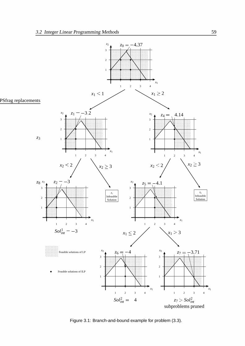
3.2 Integer Linear Programming Methods 59
1
2
3
1 2 3 4
1
2
3
1 2 3 4
1
2
3
1 2 3 4
1
2
3
1 2 3 4
1
2
3
1 2 3 4
1
2
3
1 2 3 4
z8
InfeasibleSolution
1
2
3
1 2 3 4
z3
InfeasibleSolution
Feasible solutions of LP
Feasible solutions of ILP
PSfrag replacements
z0 6 4 37
z1 6 3 2
z2 6 3
z3
z4 6 4 14
z5 6 4 1
z6 6 4 z7 6 3 71
z8
x1x1
x1 x1
x1x1
x1
x2x2
x2 x2
x2x2
x2
x1 3 1
x2 3 2 x2
3
x1
2
x2 3 2
x1 3 2 x1
3
x2
3
Sol1int 6 3
Sol2int 6 4 z7 4 Sol2
intsubproblems pruned
Figure 3.1: Branch-and-bound example for problem (3.3).

60 3. Optimization Models and Algorithms
The solution to the integer programming problem is determined when the whole tree has
been traversed, and implicitly (or explicitly) all solutions have been enumerated. The optimal
solution is the best solution found during the tree traversal. Figure 3.1 shows the search tree
resulting from the branch-and-bound method for the following ILP problem:
minimize z 6 x16 x2
subject to 1 20 x16 x2
6 16 1 43 x16 x2
6 5 (3.3)
and x
0
x is integer
For each subproblem it is indicated the feasible region (shadowed areas for the linear pro-
gramming relaxation of (3.3) and black dots for the ILP problem), and the cost function
value, zi, obtained by the Simplex method. This solution is used as an estimated lower
bound for the objective function of the ILP problem. The first solution of the linear program-
ming relaxation of (3.3) is non-integer (x1 1 52 and x2 2 85 that imply z0 6 4 37).
Considering that we select x1 to split the original problem, the search space can be divided
in two areas, one for x1 3 1 and another for x1
2, which start a tree of subproblems. This
process is repeated until the whole search space becomes implicitly or explicitly enumerated.
The first integer solution found, Sol1int z2 6 3, is saved until a better solution is found,
Sol2int z6 6 4. Note that since the lower bound estimated for z7 6 3 71 is greater than
the previous computed integer solution (Sol2int 6 4) there is no need to search for a solution
in the feasible region of that subproblem, thus the search is pruned at this node. Moreover,
a depth-first search is used in this example but other search approaches can be used, such as
breadth-first search or best-bound search [Russell 94].
3.2.2 Cutting Plane Methods
Cutting planes methods for general integer programming problems were first proposed
by Gomory [Gomory 58, Gomory 63]. These methods find exact solutions for integer pro-

3.2 Integer Linear Programming Methods 61
Feasible solutions of ILPFeasible solutions of LP
1
2
3
1 2 3 4
1
2
3
1 2 3 4
1
2
3
1 2 3 4
PSfrag replacements
z0 6 4 37 z1 6 4 10 z2 6 4
x1x1x1
x2x2x2
Initial problem Constraints added:Constraints added:
x2 3 2 x2 3 2 and x1 3 2
Figure 3.2: Cutting plane example for problem (3.3).
gramming problems by solving a sequence of linear programming relaxations of the original
problem. As noted before, the optimum solution to the LP relaxation problem, where the
integer constraints are dropped, is a lower bound on the optimum integer solution. So, if the
optimal solution to the LP relaxation problem is feasible (all the constraints are satisfied by
the solution) for the integer programming problem, the original integer linear programming
problem is solved. But, while an integer solution is not found, each iteration of cutting plane
algorithms deduces a set of new inequalities, from the original constraint requirements, to
create a new linear programming problem. These extra constraints are inferred in such a
way that no feasible integer solutions are excluded, the feasible solution region is actually
reduced and the optimum solution for the linear programming problem will contribute to an
integer solution. Using these methods it is possible to solve an integer linear program in a
finite number of iterations. However, for hard instances this finite convergence is known to
be slow, because an exponential number of cutting planes must be added [Mitchell 98b]. For
these hard integer programming instances that can not be solved to an optimum solution,
cutting planes algorithms can produce approximations to the optimum solution in moderate
computation time, with guarantees on the distance to the optimum [Mitchell 98b].
Figure 3.2 shows an example of using cutting plane methods for computing the solution
to the ILP problem described by (3.3). In each iteration of the algorithm new constraints

62 3. Optimization Models and Algorithms
are added in order to reduce the feasible solution of the LP relaxation problem but without
excluding any integer solution. The solution to the ILP problem is obtained when the solution
to the LP relaxation problem respects the integrality constraints, i.e. all xi are integers.
3.2.3 Other Approachs
Integer linear programming problems can also be solved using a combination of cutting
plane methods with branch-and-bound methods [Mitchell 94, Beasley 96]. These methods,
called branch-and-cut, work by solving a sequence of linear programming relaxations of
the integer programming problem. Cutting plane methods improve the solution of the LP
relaxation problem, introducing additional constraints which will approximate the relaxed
solution to the solution of the ILP problem, and the branch-and-bound methods proceed
using a wise divide-and-conquer approach to solve ILP problems [Mitchell 98a].
Another class of algorithms for solving integer linear programming problems are the
group theoretic. A detailed description of these algorithms, which are based on group theory,
can be found in [Salkin 75]. However, due to the complexity of these algorithms, only small
problems can be solved using these approaches [Salkin 75].
3.3 Methods for Zero-One ILPs
As noted before, an integer linear programming problem in which all variables are con-
strained to be 0 or 1 (binary variables where each xi 0 1 ) is called a zero-one integer
linear programming (ZOILP) problem. The zero-one ILP problem can be formalized using
the following matrix notation:
minimize c xsubject to A x b (3.4)
and xi 7 0 1 i 1 n

3.3 Methods for Zero-One ILPs 63
where A, b, c, and x, have the same meaning as in (3.1), except that the n problem variables
xi are now constrained to assume binary values (0,1) by the last constraint in (3.4).
A significant number of combinatorial and logical constraints can be modeled
through the use of zero-one variables. In particular, it is possible to map any integer lin-
ear programming problem, in which the variables are bounded above, as an zero-one integer
linear programming problem [Papadimitriou 83].
Any algorithm for solving ILP problems can also be used for solving zero-one ILP prob-
lems. Observe that, using a generic ILP solver for zero-one ILP problem requires that for
each variable two additional constraints be included in the formulation i.e. xi
0 and xi 3 1
for i 1 n, which guarantee that each variable value is limited to 0 or 1. However,
due to the special characteristics of zero-one integer linear programming problems (binary
variables, finite number of possible solutions), they are more suitable to be solved using
dedicated search algorithms than using general ILP algorithms. In particular, propositional
satisfiability (SAT) search algorithms can be adopted for solving zero-one ILP problems, as
will be illustrated later on.
In [Barth 95], Peter Barth described how to solve zero-one integer linear programming
problems using a propositional satisfiability (SAT) search algorithm. However, the algorithm
described in [Barth 95] is based on the Davis-Putnam search procedure [Davis 60], which has
been shown to be particularly inefficient for a large number of instances of SAT [Silva 96b].
In this section we describe two different algorithms for solving zero-one integer linear
programming problems. Both algorithms are based on SAT algorithms that solve proposi-
tional formulas generally represented in Conjunctive Normal Form (CNF). As explained in
Chapter 2 (see section 2.2 on page 25), a conjunctive normal formula ϕ denotes a boolean
function f : 0 1 n 0 1 , which is composed exclusively by a conjunction of clauses
where each clause ω is a disjunction of literals, and a literal l is either a variable xi (positive
literal) or its complement : xi (negative literal). For example, the following formula
ϕ x1 x2 _: x3 4: x1 _: x3
4: x2 _: x3 (3.5)
has 3 clauses and uses 5 literals, x1 x2 : x1 : x2 : x3 , from a set of 3 variables, x1 x2 x3 .
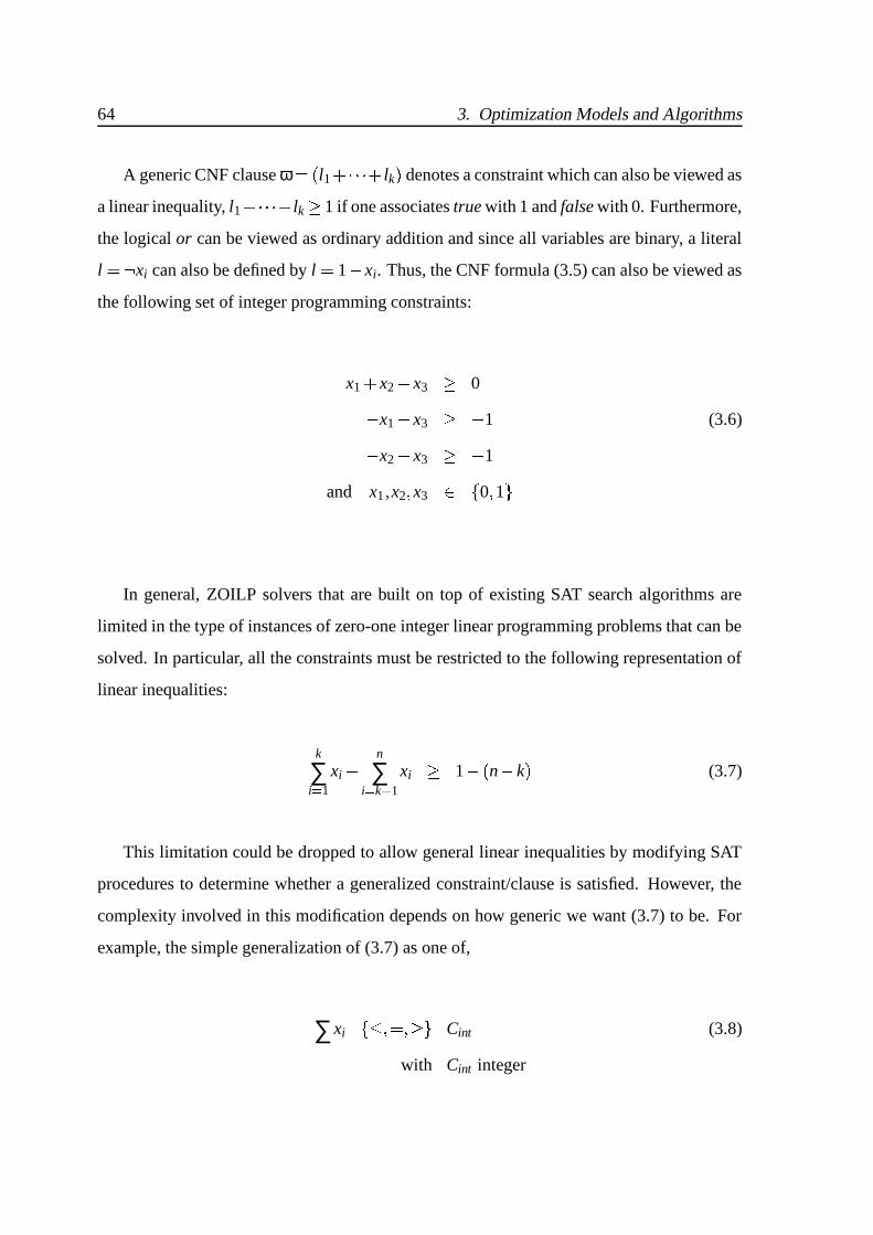
64 3. Optimization Models and Algorithms
A generic CNF clause ω l1 P lk denotes a constraint which can also be viewed as
a linear inequality, l1 P lk
1 if one associates true with 1 and false with 0. Furthermore,
the logical or can be viewed as ordinary addition and since all variables are binary, a literal
l : xi can also be defined by l 1 6 xi. Thus, the CNF formula (3.5) can also be viewed as
the following set of integer programming constraints:
x1 x26 x3
06 x1
6 x3 6 1 (3.6)6 x2
6 x3 6 1
and x1 x2 x3 0 1 In general, ZOILP solvers that are built on top of existing SAT search algorithms are
limited in the type of instances of zero-one integer linear programming problems that can be
solved. In particular, all the constraints must be restricted to the following representation of
linear inequalities:
k
∑i 1
xi6 n
∑i k 5 1
xi
1 6 n 6 k (3.7)
This limitation could be dropped to allow general linear inequalities by modifying SAT
procedures to determine whether a generalized constraint/clause is satisfied. However, the
complexity involved in this modification depends on how generic we want (3.7) to be. For
example, the simple generalization of (3.7) as one of,
∑xi 63 Cint (3.8)
with Cint integer

3.3 Methods for Zero-One ILPs 65
is conceptually straightforward to implement, but the generalization of (3.7) as a generic
zero-one integer linear programming constraint, represented by
∑ai xi 63 Creal (3.9)
with ai Creal R
is complex because it implies the re-implementation of most procedures of SAT algorithms
to handle constraints with generic coefficients. However, as we will see in the remaining
chapters of this thesis, the proposed test optimization models proposed in this work are not
limited by the restriction imposed by (3.7), because most of the models are derived from
constraints described as CNF formulas.
The first zero-one ILP solver algorithm presented in this section follows Peter Barth’s ap-
proach [Barth 95], whereas the second builds a branch-and-bound procedure on top of a SAT
engine. As we will see, by the results presented in Section 3.4, the SAT algorithm impacts di-
rectly the performance of the zero-one ILP solver. Therefore, it is crucial to use a state-of-art
SAT algorithm which includes efficient pruning techniques. For this reason, both zero-one
ILP algorithms use the GRASP SAT algorithm described in [Silva 96b], which includes sev-
eral pruning techniques for reducing the amount of search associated with instances of SAT.
Among the pruning techniques included in GRASP, the following have been shown to be
particularly significant: GRASP implements a non-chronological backtracking search strategy2.
This backtracking strategy potentially permits skipping over large portions of the de-
cision tree for some instances of SAT. GRASP utilizes selective clause recording techniques. During the search process,
and as conflicts are diagnosed (i.e. due to an assignment a clause becomes false or
2Some variations of this strategy are also commonly referred to as dependency-directed backtracking and
back-jumping [Russell 94].

66 3. Optimization Models and Algorithms
unsatisfied), new clauses are created from the causes of conflicts. These clauses rep-
resent implicates of the boolean function associated with the CNF formula, and are of-
ten referred to as nogoods [Stallman 77, Schiex 96]. Newly recorded clauses are then
used for pruning the subsequent search. Moreover, bounds on the size of recorded
clauses can be imposed, thus preventing an excessive growth of the resulting CNF
formula. In most practical situations, instances of SAT can have highly structured CNF rep-
resentations. The intrinsic structure of these representations can be exploited by
GRASP, after diagnosing the causes of conflicts, by identifying necessary assign-
ments required for preventing conflicts from being identified during the subsequent
search. In addition, other pruning techniques can be straightforwardly applied to SAT algo-
rithms. In particular, and as described in [Silva 97a], several techniques commonly
used in algorithms for different variations of the set covering problem [Coudert 96],
such as dominance relations and dynamic partitioning, can be applied. Dominance
relations between clauses identify which clauses can be deleted because they are
dominated by other clauses. A clause ω2 dominates another clause ω1 if the set
of all assignments that satisfy ω1 include the set of all assignments that satisfy ω2.
Consider for example the following two clauses ω1 x1 ò: x2 x3 s: x4 and
ω2 x1 f: x4 . Clause ω2 dominates ω1, which can be deleted because, when-
ever ω2 is satisfied, ω1 is also satisfied. Dynamic partitioning identifies disjoint
sub-formulas during the search process, that correspond to subproblems whose so-
lution can be computed separately. For example in the following CNF formula,
ϕ x0 x1 x6 ! x1 p: x2
!4: x1 x3 ! x4 x5 p: x6
!4: x4 x6 , for the as-
signment x0 1 the set of clauses involving the variables x1, x2 and x3 becomes
disjoint from the set of clauses involving the variables x4, x5 and x6. Hence, the two
sub-formulas can be solved independently.
The SAT-based algorithms presented in the next sub-sections solve zero-one ILPs as-

3.3 Methods for Zero-One ILPs 67
sociated with instances of the minimum-size prime implicant problem3. The minimum-size
prime implicant problem is defined as the problem of computing a minimum-size assignment
(in the number of literals) that satisfies a given boolean function f ; in our case f is described
in CNF format. Note that solving this problem corresponds to identifying a maximum-size
cube for function f . Minimum-size prime implicants find applications in many areas in-
cluding Electronic Design Automation (EDA). As we will see in Chapter 4, the computation
of the minimum-size test patterns, in automatic test pattern generation, can be viewed as
a particular case of computing a minimum-size prime implicant of a boolean function. In
other areas, the interest on computing minimum-size prime implicants of a boolean func-
tion has motivated extensive research work, as illustrated by the bibliographic references of
[Ngair 93, Pizzuti 96].
We used the zero-one ILP formulation described in [Silva 97c] to generate instances for
computing the minimum-size prime implicants of a Boolean function described in CNF.
Given a CNF formula ϕ, which is defined on a set of variables x1 xn , with p clauses ω1 ωp , and which denotes a Boolean function f : 0 1 n 0 1 , apply the following
transformation:
1. Create a new set of boolean variables y1 y2n , where y2i / 1 is associated with
literal xi, and y2i is associated with literal : xi.
2. For each clause ωk l1 J lm , replace each literal l j with y2i / 1 if l j xi, or with
y2i if l j : xi.
3. For each pair of variables, y2i / 1 and y2i, require that at most one is set to one. Hence,
y2i / 1 y2i 3 1.
4. The set of inequalities obtained from steps 2 and 3 can be viewed as a single set of
inequalities A y b. Furthermore, define the cost function to be,
minimize2n
∑i 1
yi (3.10)
3Note that the minimum-size prime implicant problem can be view as a specific application of the generic
binary cover problem (BCP) [Coudert 96].

68 3. Optimization Models and Algorithms
The complete ILP formulation for the minimum-size prime implicant is thus defined as
follows:
minimize2n
∑i 1
yi
subject to A y b (3.11)
and yi 7 0 1 i 1 2n
3.3.1 SAT-Based Linear Search Algorithm
The min-prime SAT-based linear search algorithm for solving ILP problems follows P.
Barth’s ILP algorithm [Barth 95] and was first described in [Silva 97c]. Let us consider the
following zero-one ILP problem:
minimizen
∑i 1
xi
subject to A x b (3.12)
and xi 0 1 i 1 nThe possible values assumed by the cost function for the different assignments to the
variables in the set x1 xn range from 0, when all variables are assigned value 0, to n,
when all variables are assigned value 1. P. Barth’s [Barth 95] approach consists of applying
the following sequence of steps, starting from an upper bound of k n on the value of the
cost function:
1. Create a new inequality ∑ni 1 xi 3 k. This inequality basically requires that a computed
solution must have no more than k literals assigned value 1.
2. Solve the resulting instance of satisfiability. (Note that this instance is defined on
linear inequalities, but as we already mentioned, modifying most SAT algorithms for
handling this generalization is straightforward.)

3.3 Methods for Zero-One ILPs 69
3. If the instance of SAT is satisfiable decrement k (i.e. specify a new value for the cost
function) and go back to step 1. Otherwise, report that the solution to the zero-one
ILP is k 1. In those cases where the initial SAT instance is not satisfied, then the
problem does not have a solution.
Note that this ILP algorithm allows for any SAT algorithm to be used as the underlying
SAT testing engine, provided the algorithm is modified to handle linear inequalities. The
proposed ILP algorithm is illustrated in Figure 3.3. For our particular case, the solve sat
function call invokes the GRASP SAT algorithm [Silva 96b].
As noted before, one distinct feature of the GRASP algorithm is non-chronological back-
tracking. However, by appending the constraint ∑ni 1 xi 3 k, involving all the variables, we
are limiting non-chronological backtracking solely to the conflicts occurring on the original
constraints of the problem, i.e. logical conflicts. Note that a conflict in the appended con-
straint will always result in a chronological backtrack because all variables are involved, and
so the analysis of the conflict will necessarily point to the last assignment. However, as we
will see in Section 3.4, the results obtained by the min-prime algorithm outperform other
non-SAT ILP solvers for most instances evaluated.

70 3. Optimization Models and Algorithms
int min prime(ϕ)
k n;
while k 0 do
ϕ ϕ 8 ∑xi 3 k ;status solve sat ϕ ;ϕ ϕ 6 ∑xi 3 k ;if (status SATISFIABLE) then
k ∑xi;
k 6 6 ;
else
k ;
break;
end if
end while
return k;
Figure 3.3: SAT-based linear search algorithm.
3.3.2 SAT-Based Branch-and-Bound Algorithm
A different algorithmic organization consists of using a variation of the branch-and-
bound procedure [Nemhauser 88], where upper bounds to the cost function of (3.12) are
identified and lower bounds to the current set of variable assignments are estimated.
The implementation of [Manquinho 97], uses the independent set based lower bound
estimation procedure described in [Coudert 96]. This technique, widely used for computing
lower bounds, consists in finding a maximum set of disjoint clauses (Dω), i.e. the maximum
number of clauses (ωk) with no literals (l j) in common between them4. The minimum cost
4If we consider a graph whose vertices are the clauses, and such that there is an edge between two
clauses if and only if they have one common literal, then the set Dω is the maximal independent set on this
graph [Coudert 96].
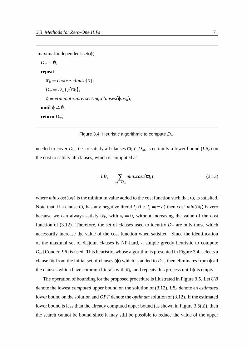
3.3 Methods for Zero-One ILPs 71
maximal independent set(ϕ)
Dw /0;
repeat
ωk choose clause ϕ ;Dw Dw 7r ωk ;ϕ eliminate intersecting clauses ϕ wk
;until ϕ /0;
return Dw;
Figure 3.4: Heuristic algorithmic to compute Dw.
needed to cover Dω, i.e. to satisfy all clauses ωk Dω, is certainly a lower bound (LBe) on
the cost to satisfy all clauses, which is computed as:
LBe ∑ωk . Dω
min cost ωk (3.13)
where min cost ωk is the minimum value added to the cost function such that ωk is satisfied.
Note that, if a clause ωk has any negative literal l j (i.e. l j : xi) then cost min ωk is zero
because we can always satisfy ωk, with xi 0, without increasing the value of the cost
function of (3.12). Therefore, the set of clauses used to identify Dω are only those which
necessarily increase the value of the cost function when satisfied. Since the identification
of the maximal set of disjoint clauses is NP-hard, a simple greedy heuristic to compute
Dω [Coudert 96] is used. This heuristic, whose algorithm is presented in Figure 3.4, selects a
clause ωk from the initial set of clauses (ϕ) which is added to Dω, then eliminates from ϕ all
the clauses which have common literals with ωk, and repeats this process until ϕ is empty.
The operation of bounding for the proposed procedure is illustrated in Figure 3.5. Let UB
denote the lowest computed upper bound on the solution of (3.12), LBe denote an estimated
lower bound on the solution and OPT denote the optimum solution of (3.12). If the estimated
lower bound is less than the already computed upper bound (as shown in Figure 3.5(a)), then
the search cannot be bound since it may still be possible to reduce the value of the upper
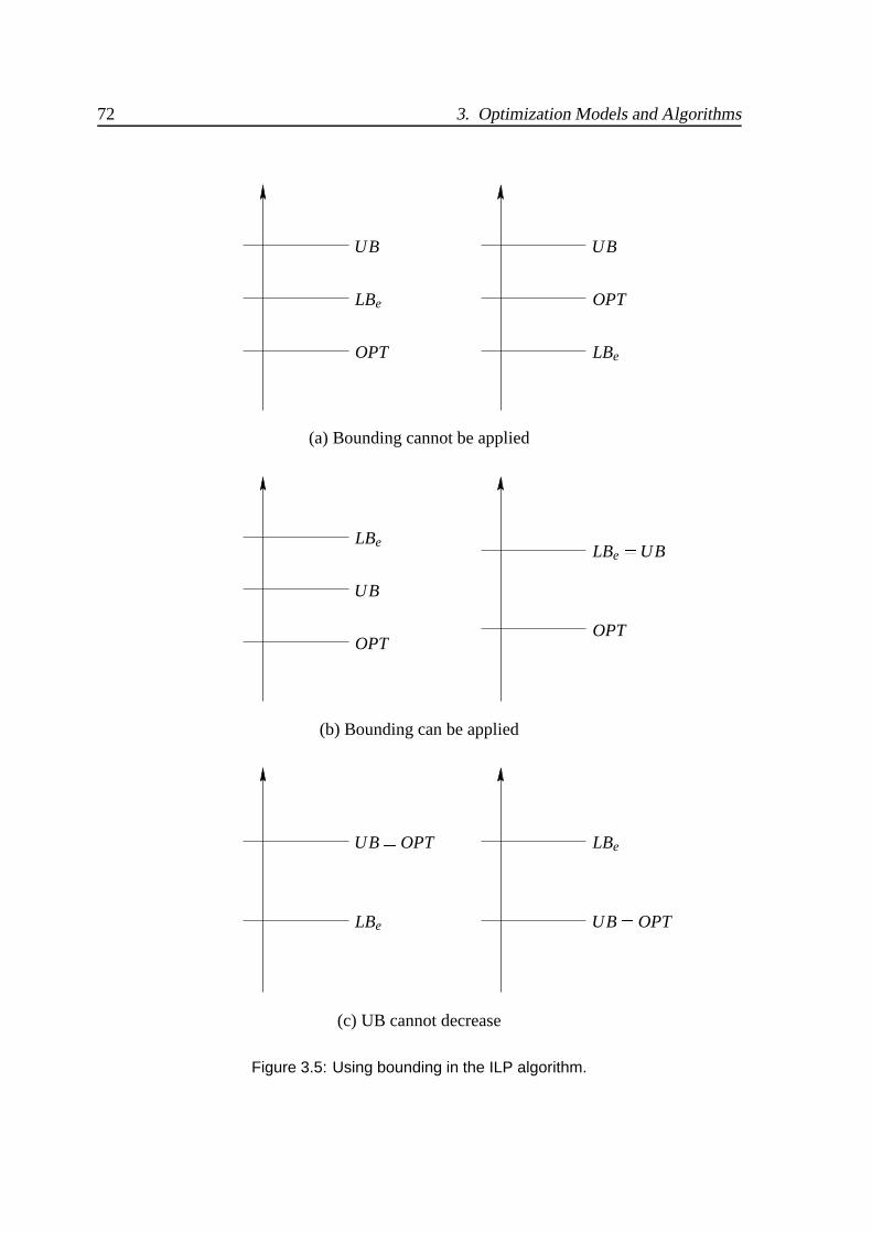
72 3. Optimization Models and Algorithms
UB
LBe
OPT
UB
OPT
LBe
(a) Bounding cannot be applied
OPT
LBe
UB
LBe UB
OPT
(b) Bounding can be applied
LBe
UB OPTLBe
UB OPT
(c) UB cannot decrease
Figure 3.5: Using bounding in the ILP algorithm.

3.3 Methods for Zero-One ILPs 73
bound. Clearly, the search can be bound whenever the estimated lower bound of the objective
function of (3.12) is larger than or equal to the existing upper bound to the solution of (3.12),
as illustrated in Figure 3.5(b). Finally, observe that Figure 3.5(c) denotes the conditions after
which the upper bound will no longer be updated during the search.
Moreover, since the branch-and-bound procedure is embedded in the SAT algorithm,
every pruning technique used by the SAT algorithm can also be used in solving the ILP.
This is particularly useful whenever a constraint of (3.12) becomes unsatisfied. The branch-
and-bound procedure, that was implemented in the bsolo solver and whose pseudo-code is
shown in Figure 3.6, consists of the following steps:
1. Initialize the upper bound to the highest possible value ( ∞).
2. If a solution to the constraints has been identified, then determine the new minimum
value of the cost function of the ILP formulation. Update the current upper bound
and issue a conflict to guarantee that the search is bound (Issue UB based con f lict).
Otherwise, branch on a given decision variable (i.e. make decision assignment).
3. Apply boolean constraint propagation [Zabih 88]. If a conflict is reached, then diag-
nose conflict, record relevant clauses, and proceed with the search process or back-
track if required.
4. Estimate lower bound. If this value is larger than or equal to the current upper bound,
then issue a conflict (Issue LB based con f lict), diagnose the conflict, backtrack, and
continue the search from step 2.
Observe that the proposed branch and bound SAT-based ILP algorithm has the following
main differences with respect to the linear search ILP algorithm: No clauses involving the cost function are created. The exception occurs when a
solution to the constraints is found or the estimated lower bound is no less than the
computed upper bound. In this situation a clause involving a subset of variables in the
cost function is temporarily created, thus causing the search procedure to backtrack.

74 3. Optimization Models and Algorithms
int bsolo(ϕ)
UB ∞;
while (TRUE) do
if Solution f ound T RUE) then
UB Cost f unction value ;Issue UB based con f lict ;
else
Decide ;end if
while (Deduce CONFLICT) do
if Diagnose CONFLICT) then
return UB;
end if
end while
while (Estimate LB UB) do
Issue LB based con f lict ;if (Diagnose CONFLICT) then
return UB;
end if
end while
end while
Figure 3.6: SAT-based branch-and-bound algorithm. Lower bounding procedures are required. As mentioned earlier, the lower bounding
procedures of [Coudert 96] are used, but lower bounding procedures based on linear
programming relaxations or lagrangian relaxation can also be used [Berkelaar 92,
Nemhauser 88]. Clearly, the tightness of the lower bounding procedure is crucial for
the efficiency of the branch-and-bound procedure.
As described, in the SAT-based branch-and-bound algorithm bsolo (Figure 3.6) there are

3.3 Methods for Zero-One ILPs 75
three types of conflicts which can arise: logical conflicts, upper bound conflicts and lower
bound conflicts. Logical conflicts, that occur when the one of the constraints of the problem
is unsatisfiable, are solved by the usual conflict analysis procedure of GRASP that determines
to which decision level the search should backtrack and if possible in a non-chronological
manner (see [Silva 96a, Silva 96b] for details of the non-chronological backtrack search SAT
algorithm). Upper bound conflicts and lower bound conflicts occur when a solution to the
constraints is found, and when the estimated lower bound is higher than or equal to the upper
bound, respectively. These bounding conflicts are treated differently than logical conflicts.
In both situations, a new clause must be added to the problem in order for a logical conflict
to be issued and, consequently, to bound the search.
The new clause, added to bound the search when a bound conflict arises, is built us-
ing the assignments that are deemed responsible for the conflict to arise. In the approach
of [Manquinho 97], the new clause is built to bound the search by including all the decision
variables in the search tree, i.e. every variable assignment xi 1 (or xi 0) will contribute
to the new clause with the literal : xi (or xi, respectively). Clearly, by construction, after
the clause is built its state is unsatisfied. Therefore, the conflict analysis procedure has to
be called to determine to which decision level the algorithm must backtrack to. This was
also the case with the SAT-based linear search algorithm (min-prime), the problem with
this approach is that backtracking is always chronological, since it depends on all decisions
made.
New ways of building these bounding clauses which enable non-chronological backtrack-
ing due to upper and lower bound conflicts are presented in [Manquinho 99, Manquinho 00b].
However, the results presented in next section show that the simple approach used in [Manquinho 97]
for building the upper and lower bound conflicts clauses have resulted in an algorithm that
has a good performance when compared to other ILP solvers, in particular, bsolo outper-
forms the min-prime algorithm in most instances. Moreover, new versions of the bsolo
algorithm (which enable non-chronological backtracking on the bounding clauses among
other pruning techniques) have been proposed and evaluated by Manquinho [Manquinho 99,
Manquinho 00b]. The results obtained with these new versions, improved our results and fur-
ther indicate that bsolo is particular efficient for solving instances of some models proposed

76 3. Optimization Models and Algorithms
in this thesis.
3.4 Experimental Results – Tool Selection
In this section we include experimental results of several integer linear programming
tools (which implement different algorithms) used for solving instances of zero-one ILPs
associated with the minimum-size prime implicant problem.
The algorithms selected for solving the resulting zero-one integer programming problem
instances include three SAT based algorithms opbdp, min-prime and bsolo. opbdp uses the
implicit enumeration algorithm described in [Barth 95], min-prime is based on linear search
through the possible values of the cost function as described in Section 3.3.1, whereas bsolo
uses the SAT based branch-and-bound algorithm described in Section 3.3.2. We also com-
pare these SAT-based ILP algorithms with other generic ILP solvers, lp-solve [Berkelaar 92],
and the commercial optimization tool CPLEX. Moreover, the binate covering tool scherzo [Coudert 96]
is also evaluated, since minimum-size prime implicant computation can also be viewed as a
restricted form of the binate covering problem. The function f for which we want to iden-
tify the minimum-size prime implicants was selected from the set of satisfiable instances of
the DIMACS benchmarks [Johnson 93]. The aim instances were randomly generated with
exactly one satisfying assignment. The ii8 instances are obtained from inductive inference
problems [Kamath 92]. The jnh instances were randomly generated to be computationally
hard to solve and the ssa are instances from circuit fault analysis (a single stuck-at fault). The
CPU times, obtained on a SUN 5/85 machine with 64 MByte of physical memory, are shown
in Table 3.1. For each benchmark and for each tool 3000 seconds of CPU time were allowed.
Table 3.2 includes the upper bound on the minimum-size prime implicant computed by each
algorithm for each benchmark. Column min indicates the size of the minimum-size prime
implicant, when this size is known. (Observe that for some of the benchmarks the minimum-
size prime implicant is still unknown.) When a tool finishes, it reports the minimum-size
prime implicant if it was identified, otherwise the lowest computed upper bound is reported
provided at least one upper bound was identified. For the results shown, whenever a tool
quits earlier than 3000 seconds, it is because the tool exceeded the limit imposed on the

3.4 Experimental Results – Tool Selection 77
Generic ILP algorithms SAT based algorithms
Benchmark CPLEX lp-solve scherzo opbdp min-prime bsolo
aim-50-1 6-y1-1 116.50 8 3000 2.33 0.09 0.05 0.07
aim-50-2 0-y1-2 109.50 8 3000 5.65 0.64 0.02 0.04
aim-50-3 4-y1-3 62.90 377.10 0.57 0.40 0.08 0.18
aim-50-6 0-y1-4 26.90 96.80 0.73 0.48 0.07 0.17
aim-100-1 6-y1-2 8 3000 8 3000 8 1000 8 3000 0.09 0.22
aim-100-2 0-y1-3 8 3000 8 3000 691.57 42.45 0.17 0.45
aim-100-3 4-y1-4 8 3000 8 3000 35.47 0.81 0.47 1.08
aim-100-6 0-y1-1 294.30 8 3000 2.78 0.18 0.32 0.52
aim-200-1 6-y1-3 8 3000 8 3000 8 345 8 3000 0.22 0.76
aim-200-2 0-y1-4 8 3000 8 3000 8 1705 8 3000 0.83 2.60
aim-200-3 4-y1-1 8 3000 8 3000 8 3000 41.84 4.32 2.31
aim-200-6 0-y1-2 8 3000 8 3000 619.38 4.59 3.58 2.76
ii8a1 63.30 786.90 0.98 1.93 861.53 3.51
ii8b2 8 3000 8 3000 8 3000 8 3000 8 3000 8 3000
ii8c2 8 3000 8 3000 8 3000 8 3000 8 3000 8 3000
ii8d2 8 3000 8 3000 8 3000 8 3000 8 3000 8 3000
ii8e2 8 3000 8 3000 8 3000 8 3000 8 3000 8 3000
jnh1 8 3000 8 3000 70.00 2.24 17.96 11.39
jnh7 8 3000 8 3000 5.35 0.45 9.06 2.88
jnh12 2529 8 3000 3.07 0.12 0.58 1.10
jnh17 873.90 8 3000 17.28 0.30 2.53 2.13
ssa7552-038 8 3000 8 3000 8 223 8 3000 8 1205 8 500
Table 3.1: CPU times on selected benchmarks.
virtual memory allowed to solve each instance (i.e. 64 MByte).
As can be concluded, general-purpose ILP solvers, such as CPLEX and lp-solve, may
be inadequate for computing minimum-size prime implicants. Similarly, despite the very
promising results as an algorithm for solving binate covering problems [Coudert 96], scherzo
performs particularly poorly when computing minimum-size prime implicants. The three
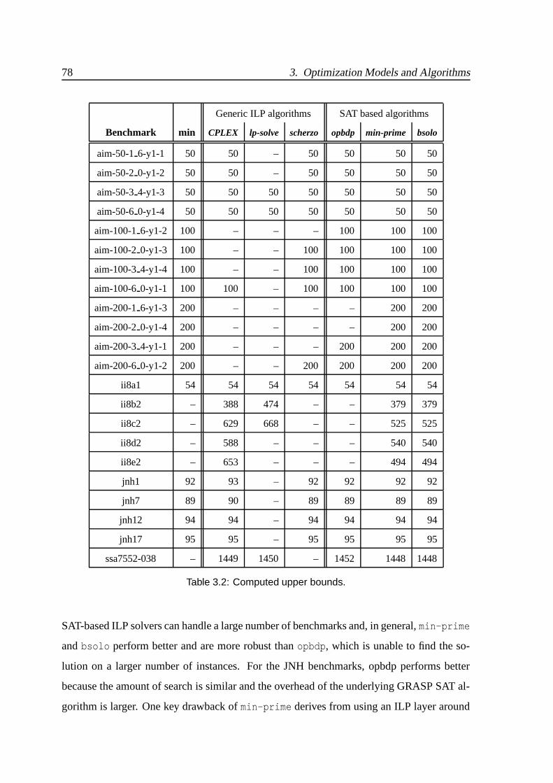
78 3. Optimization Models and Algorithms
Generic ILP algorithms SAT based algorithms
Benchmark min CPLEX lp-solve scherzo opbdp min-prime bsolo
aim-50-1 6-y1-1 50 50 – 50 50 50 50
aim-50-2 0-y1-2 50 50 – 50 50 50 50
aim-50-3 4-y1-3 50 50 50 50 50 50 50
aim-50-6 0-y1-4 50 50 50 50 50 50 50
aim-100-1 6-y1-2 100 – – – 100 100 100
aim-100-2 0-y1-3 100 – – 100 100 100 100
aim-100-3 4-y1-4 100 – – 100 100 100 100
aim-100-6 0-y1-1 100 100 – 100 100 100 100
aim-200-1 6-y1-3 200 – – – – 200 200
aim-200-2 0-y1-4 200 – – – – 200 200
aim-200-3 4-y1-1 200 – – – 200 200 200
aim-200-6 0-y1-2 200 – – 200 200 200 200
ii8a1 54 54 54 54 54 54 54
ii8b2 – 388 474 – – 379 379
ii8c2 – 629 668 – – 525 525
ii8d2 – 588 – – – 540 540
ii8e2 – 653 – – – 494 494
jnh1 92 93 – 92 92 92 92
jnh7 89 90 – 89 89 89 89
jnh12 94 94 – 94 94 94 94
jnh17 95 95 – 95 95 95 95
ssa7552-038 – 1449 1450 – 1452 1448 1448
Table 3.2: Computed upper bounds.
SAT-based ILP solvers can handle a large number of benchmarks and, in general, min-prime
and bsolo perform better and are more robust than opbdp, which is unable to find the so-
lution on a larger number of instances. For the JNH benchmarks, opbdp performs better
because the amount of search is similar and the overhead of the underlying GRASP SAT al-
gorithm is larger. One key drawback of min-prime derives from using an ILP layer around

3.4 Experimental Results – Tool Selection 79
the SAT algorithm which creates large additional clauses. For the minimum-size prime im-
plicant problem, these additional clauses involve all variables in the problem representation.
Hence, conflicts involving this clause necessarily lead to chronological backtracking to the
most recent decision assignment [Silva 96a, Silva 96b], and so the most useful features of
GRASP cannot be exploited. Finally, we note that bsolo tends to be a more efficient search
algorithm than min-prime, as the experimental results suggest. For this reason we choose
the bsolo ILP solver for solving the ILP optimization models proposed in the remainder of
this thesis.

80 3. Optimization Models and Algorithms
3.5 Conclusions
In this chapter we briefly presented the main approaches for solving the integer linear
programming problem. In particular, we concentrated on satisfiability-based algorithms for
solving zero-one ILP problem instances. We described algorithms for computing the mini-
mum size prime implicant of boolean functions. The model is based on an ILP formulation
and the proposed algorithms are built on top of existing SAT solvers, in our case GRASP.
The algorithms, min-prime and bsolo, are based on the well known linear search algo-
rithm and the branch-and-bound method, respectively. To our best knowledge min-prime
and bsolo are the first SAT-based ILP algorithms that incorporate conflict diagnosis tech-
niques [Silva 96b] in solving optimization problems. Both algorithms incorporate several
powerful search-pruning techniques which are known to be particularly useful for SAT algo-
rithms, in particular the non-chronological backtracking strategy, the clause (nogood) record-
ing procedures, and the identification of necessary assignments.
As the results given in the previous section clearly show, the proposed algorithms are
the most competitive for the set of benchmarks considered. Moreover, those results also
show that, for these classes of benchmarks, the branch and bound SAT-based ILP algorithm
bsolo is in general more efficient than the SAT-based linear search algorithm, min-prime.
Therefore, we selected the bsolo ILP solver for solving the ILP optimization models pro-
posed in the remainder of this thesis. Recent research [Manquinho 99, Manquinho 00a,
Manquinho 00b] confirms this choice: new versions of the bsolo SAT-based linear search
algorithm outperform the other solvers (presented in Table 3.2) for the test optimization in-
stances that result from the models proposed in this thesis, in particular, for the minimum
size test pattern generation model proposed in Chapter 5.
Having described the optimization models and algorithms for solving them, which will
be used in the remainder of this thesis, we are now in condition to present the proposed
optimization models for testing problems. In the next chapter, we will describe an ILP
optimization model that identifies a complete minimum test set for arbitrary combinational
circuits.
Chapter 4
Test Set Compaction Models
Contents
4.1 Introduction
4.2 Minimum Size Test Set – Reference Model
4.2.1 Irredundant Combinational Circuits
4.2.2 Arbitrary Combinational Circuits
4.2.3 Practical Considerations
4.3 Minimum Size Test Set – Proposed Model
4.3.1 Irredundant Combinational Circuits
4.3.2 Arbitrary Combinational Circuits
4.3.3 Practical Considerations and Other Improvements
4.4 Maximum Test Set Compaction
4.4.1 Set Covering Model for Test Compaction
4.4.2 Experimental Results
4.5 Conclusions
81

82 4. Test Set Compaction Models

4.1 Introduction 83
4.1 Introduction
Test set compaction is a fundamental problem in digital system testing. The test size
(number of vectors) is directly related with the time and cost of test application during the
production phase. For economical reasons a compact test set is highly desirable, even if it
is necessary to use a heavily computational effort during the test generation process or in an
additional test set reduction process, or both.
As seen in the previous chpater, the ATPG process for digital circuits has been extensively
investigated and most of the algorithms are able to generate a complete test set for a given cir-
cuit [Goel 81, Fujiwara 83, Kirkland 87, Schulz 88, Silva 94, Stephan 96, Silva 97b]. How-
ever, only during the last decade did the problem of deriving small test sets gain key impor-
tance due to the increasing complexity of the circuits and large scale production. The ideal
goal is to obtain the minimum number of test vectors that detect all the detectable faults in
an arbitrary combinational circuit. This problem is computationally hard and its restriction
to the subset of irredundant circuits is known to be NP-hard [Krishnamurthy 84]. Neverthe-
less, many competitive solutions have been proposed, most of which based on heuristic ap-
proaches [Pomeranz 91, Reddy 92, Pomeranz 93b, Chang 95, Kajihara 95, Hamzaoglu 98].
In this chapter we propose an integer linear program (ILP) model for solving the min-
imum test set problem. The proposed formulation is polynomial in the size of the circuit.
To our best knowledge, only two other approaches [Matsunaga 93, Silva 98] have proposed
non-heuristic solutions to the minimum test set problem for arbitrary combinational circuits.
In [Matsunaga 93] the problem is formalized as a minimum set cover problem, and then im-
plicit manipulations techniques using binary decision diagrams (BDDs) are applied. Given
that this approach is based on implicitly representing all test patterns for each fault, it re-
quires worst-case exponential space, and so it is impractical except for very small circuits.
[Silva 98] proposes an integer linear programming model in which the size of representation
is polynomial in the size of the circuit representation. Our proposed model is closely related
with the techniques proposed in [Silva 98], henceforth referred to as the reference model,
which are based on the SAT model presented in Section 2.3.2. Although our model has the
same worst-case polynomial size representation of the reference model, it significantly im-

84 4. Test Set Compaction Models
proves on its representation size. Moreover, we propose additional techniques for reducing
the size of the proposed ILP formulation for practical circuits. These techniques include the
identification of fault independence relations, removal of redundant faults by preprocessing,
using empirical upper bounds, and limiting the model to the nodes related with each fault.
Using these techniques the new model can be used to obtain optimal solutions for small-size
circuits. Hence, besides its theoretical interest, the proposed model can be used to validating
new and existing test set compaction heuristics.
However, for larger circuits this model becomes impractical. Therefore, we developed
a practical alternative approach using a post-generation compaction method, and studied
the effect of fault simulation in the test set compaction. The existing heuristic approaches,
which do not guarantee to compute a test set of minimum size, perform in practice extremely
well [Hamzaoglu 98, Pomeranz 93b]. For heuristic approaches, and given a pre-computed
test set which is not known to be optimum, one can potentially remove redundant test pat-
terns, thus obtaining a reduced test set. Clearly, this reduced test set need not be the minimum
size test set for the circuit. The existence of redundant tests is intrinsic to any heuristic ATPG
tool, since in general any fault simulation strategy is unable to guarantee the complete elim-
ination of redundant test patterns. One approach for minimizing a pre-computed test set has
been proposed by D. Hochbaum in [Hochbaum 96], and consists of casting the problem of
removing redundant test patterns from a test set as an instance of the set covering problem.
Since the set covering problem can naturally be formulated as a 0-1 integer linear program,
an integer programming approach based on linear programming relaxations was proposed
and evaluated in [Hochbaum 96]. Nevertheless, only very preliminary experiments were
conducted. In particular, the effect of fault simulation on the ability of reducing the size of
a test set was not evaluated. Therefore in this chapter we also study the application of set
covering models to the compaction of test sets, which can be used over any heuristic test set
compaction procedure. For this purpose, recent and highly effective set covering algorithms
are used [Coudert 96]. Experimental evidence suggests that the size of the computed test sets
can often be reduced by using set covering models and algorithms. Moreover, a noteworthy
empirical conclusion is that it may be preferable not to use fault simulation when the final
objective is test set compaction.

4.2 Minimum Size Test Set – Reference Model 85
This chapter is organized as follows. In the next section we present the reference model
for computing the minimum size test set. In the Section 4.3 we describe in detail the proposed
ILP model and present results showing that our model has a smaller size representation.
Finally in Section 4.4 we describe the set covering model for test set compaction and present
some experimental results of the test set compaction model.
4.2 Minimum Size Test Set – Reference Model
In this section we introduce the reference model for the computation of the minimum
number of test patterns which detects all detectable faults in a combinational circuit [Silva 98].
First, we provide an ILP formulation for computing the minimum number of test patterns
which detect all faults in an irredundant circuit. Afterwards, we extend this formulation to
arbitrary combinational circuits, which may include redundant faults.
4.2.1 Irredundant Combinational Circuits
The first problem we address is to identify the minimum number of test patterns that
detect all faults in an irredundant combinational circuit. Let us consider a circuit where
there are M stuck-at faults to be detected. So, we need at least to specify M fault detection
formulas, one for each fault. Moreover, M tests suffice for detecting all M faults. As a result,
we can create M copies of each circuit formula, and for each such formula we can create
M associated fault-specific formulas, one for each fault. A set of tests that detects all faults
will do so in such a composed formula. Figure 4.1 shows the global organization of this
approach for detecting all stuck-at faults. In each copy of the good circuit ϕGi , each node
variable x will be represented as xGi . Accordingly, in each copy a fault-specific formula ϕFS
i j ,
the variables associated with fault detection problems and with node x will be represented as
xFi j, for the faulty node, and xS
i j, for the sensitization node. Given the above, the problem of
minimizing the number of tests is now reduced to finding a set of test patterns that detects all
faults and that minimizes the number of copies ϕGi that are required. Note that the values on
the primary inputs of each used copy ϕGi are the minimum size test set.
Let us associate a Boolean variable di j with each fault-specific formula ϕFSi j which as-

86 4. Test Set Compaction Models
9;:< = >@?+>@A@?+B(C#?EDGFHBI?(J KLC,MONP?QB
R;ST U V@W+V@X@W+Y(Z#WE[G\HYIW(] ^LZ,_O`PWQY
a;bc d e@f+e@g@f+h(i#fEjGkHhIf(l mLi,nOoPfQh
prqtsuv u
wrxtyz |
r~t
rt
rt
rt
rt
rt ¡
¢r£t¤¥ ¦ ¥
Figure 4.1: Global formula organization for detecting all faults.

4.2 Minimum Size Test Set – Reference Model 87
sumes value true whenever fault j is detected with copy i of the circuit formula and associ-
ated fault-specific formula. This leads to the following conditions for all i, j:,x . PO
xSi j di j ,
x . PO
: xSi j di j ,
x . PO
di j 6 xSi j 0 (4.1)
and,
di j ∑x . PO
xSi j : di j ∑
x . PO
xSi j ∑
x . PO
xSi j 6 di j 0 (4.2)
Hence, fault j is detected with ϕFSi j , if at least one sensitization xS
i j variable (with x PO)
evaluates to true. In addition, either di j assumes value 0, or the error signal must reach at
least one primary output; hence condition (4.2). Clearly, since each fault j is detectable and
must be detected by a test set, then the following conditions must hold,
M
∑i 1
di j M
∑i 1
di j 1 (4.3)
for j 1 M . Let us now introduce a variable si j, for each variable di j, such that,
§di j si j ¨ § : di j si j ¨ si j 6 di j 0 (4.4)
and, for all i 2 M j 1 M §si / 1 j si j ¨ § : si / 1 j si j ¨ si j 6 si / 1 j 0 (4.5)
Variable si j evaluates to true whenever di j 1. In such a situation, for all k 4 i, sk j 1.
Thus, each variable si j permits selecting the least i for which fault j is detected. Notice that
the least i for which fault j is detected is such that si / 1 j 0 and si j 1.

88 4. Test Set Compaction Models
In addition to the previous variables, we need to associate a Boolean variable ui that is
assigned value true whenever copy i of the circuit formula is used to detect at least one fault
which had not been detected with a smaller i. Hence, we must have,
§s1 j u1 ¨ § : s1 j u1 ¨ u1
6 s1 j 0 (4.6)
for j 1 M , and
§ si / 1 j ) si j ui ¨ § :P: si / 1 j si j ui ¨ si / 1 j 6 si j ui
0 (4.7)
for i _ 2 M and j _ 1 M . This condition basically states that the first copy i,
for which fault j is detected, is declared to be used for detecting fault j. Hence, from the
definition of ui we have the following result,
Proposition 4.1 Given the definition of ui in (4.6) and (4.7), each fault j can set exactly one
variable ui to true. Moreover, more than one fault j can set the same variable ui.
Finally, we must define the cost function that we want to minimize. Clearly, this cost
function should minimize the number of copies of the circuit formula that are used for de-
tecting all faults, and so we get,
minM
∑i 1
ui (4.8)
The M replicas of the clausal representation of the circuit, each with its M copies of the
fault detection problems, as well as (4.1) through (4.8) capture the problem of computing
the minimum number of tests for a given irredundant circuit. For the C17 benchmark circuit
(see Figure 2.4 on page 26), which have 34 non-collapsed stuck-at fault, the data for the
associated ILP formulation is summarized in Table 4.1. Finally, in [Silva 98] and [MS 97]
the following formal results have been established and proven.

4.2 Minimum Size Test Set – Reference Model 89
# Clauses # Formulas
Circuit formula ϕG 34
Fault-specific formula ϕFS 342 1156
Fault detection (4.1) (4.2) 342 1156
Detection requirement (4.3) 34
Fault detection selection (4.4) 342 2312
Propagation of selection (4.5) 33 " 34 1122
Usage of replica i (4.6) (4.7) 34 33 " 34 1156
Cost function (4.8) 1
Table 4.1: Upper bounds on the ILP formulation for the C17 benchmark circuit.
Proposition 4.2 The size of the ILP for the minimum test set problem (described above) is
O M2 N O N3 .Proposition 4.3 The minimum value of (4.8) denotes the minimum number of tests that de-
tect all faults in the irredundant combinational circuit C. Furthermore, each of the assign-
ments to the primary inputs of each circuit copy ϕGi , for which ui 1, denote a test pattern.
4.2.2 Arbitrary Combinational Circuits
The next problem addressed is the identification of the minimum number of test patterns
which detect all detectable faults in a given arbitrary combinational circuit, as well as the
identification of all the redundant faults in that circuit. This problem is quite similar to the
problem of the previous section, with the added difficulty that some faults are now redundant.
One simple solution to this problem is to introduce additional variables and modify some
of the equations of the ILP of the previous section. First, let us define a variable r j, with
j 1 M , that is true when fault j is declared redundant. Given that some faults are
indeed redundant, constraint (4.3) must be modified to capture this fact:
M
∑i 1
di j r j M
∑i 1
di j r j
1 (4.9)

90 4. Test Set Compaction Models
for j 1 M . This condition requires that either the fault is detected by at least one
copy of the circuit formula or otherwise it must be declared redundant. The next step is to
modify the cost function so as to penalize the existence of redundant faults. This can be
done by giving a sufficiently large weight to variables declared redundant, such that the cost
of declaring a fault redundant is larger than the sum of all ui variables. Hence, the minimum
value is achieved only when the actual redundant variables are declared redundant, since
these faults cannot be detected. Consequently, we obtain the following cost function:
min M
∑i 1
ui M M
∑j 1
r j (4.10)
This cost function splits the range of possible values into disjoint sets according to the
number of variables r j set to true. Valid ranges are (1 to M) for no redundant faults, (M 1
to 2 M 6 1) for one redundant fault, (2 M 1 to 3 M 6 2) for two redundant faults, etc.
The size of these ranges is, respectively, M, M 6 1, M 6 2, etc. Intuitively, the minimum
value will be achieved when all detectable faults are indeed detected and in the least number
of copies of the circuit formula. The ILP formulation for this problem is summarized in
Table 4.2.
Proposition 4.4 The minimum value of (4.10), assuming (4.9) instead of (4.3), denotes the
minimum number of tests that detect all detectable faults and identify all redundant faults in
a combinational circuit C. In addition, the assignments to the primary inputs of each circuit
copy ϕGi , for which ui 1, denote a test pattern. Finally, each variable r j set to true indicates
that fault j is redundant.
4.2.3 Practical Considerations
In practice the size of the model can be reduced because we do not need to consider all
possible circuit faults nor to assume that one vector detects at least only one fault. Different
techniques for reducing the size of the ILPs associated with minimum test set computation
are described in [MS 97, Silva 98]. These techniques involve removing redundant faults from

4.2 Minimum Size Test Set – Reference Model 91
Clauses Ranges of indices
Circuit representation ϕGi 1 3 i 3 M
Fault-specific representation ϕFSi j 1 3 i 3 M, 1 3 j 3 M
Fault detection
,x . PO
di j 6 xSi j 0 1 3 i 3 M, 1 3 j 3 M
∑x . PO
xSi j 6 di j 0 1 3 i 3 M, 1 3 j 3 M
Detection requirementM
∑i 1
di j r j
1 1 3 j 3 M
Fault detection selection si j 6 di j 0 1 3 i 3 M, 1 3 j 3 M
Propagation of selection si j 6 si / 1 j 0 2 3 i 3 M, 1 3 j 3 M
Usage of replica iu16 s1 j 0 1 3 j 3 M
si / 1 j 6 si j ui
0 2 3 i 3 M, 1 3 j 3 M
Cost function to minimizeM
∑i / 1
ui M M
∑j 1
r j
Table 4.2: ILP for the minimum test set problem.
the fault set, applying fault dominance and independence relationships, and using empirical
upper bounds. Applying to the model such techniques we are reducing the values of the
M, which limit the range of indices i and j. For example, in the benchmark circuit C17,
there are a total of 34 stuck-at faults. This leads to the ILP model described in Table 4.1. In
contrast, by running the ATPG algorithm ATALANTA [Lee 93], four test patterns are identified.
Thus, instead of an ILP model that contains 342 1156 fault-specific formulas, using the
empirical upper bound of 4 tests the number of fault-specific formulas is guaranteed to be at
most 4 " 34 136. Moreover, by taking into account dominance relations, the set of faults
can be collapsed into 17 faults [Brglez 85]. Thus, only 17 " 4 68 fault-specific formulas
need to be considered. Similarly, the number of fault detection formulas is also reduced to
17 " 4 68. Likewise, the number of all other clauses used in the ILP formulation are also
reduced once the range of i and j indices are narrowed to 1 3 i 3 4 and 1 3 j 3 17, because
we need at most 4 vectors and there are only 17 collapsed faults, respectively.

92 4. Test Set Compaction Models
4.3 Minimum Size Test Set – Proposed Model
In this section we propose a new model for the computation of the minimum number of
test patterns which detects all detectable faults in a combinational circuit. The new model
also has size complexity O N3 , but, as we will see, for most circuits the effective size of its
ILP formulation is significantly smaller than the size of the ILP used in the reference model.
In fact, this is true for all circuits where the number of nodes is much bigger than the number
of primary inputs and outputs, a condition which is verified by most practical circuits. As
in the previous section, first we provide an ILP formulation for computing the minimum
number of test patterns which detect all faults in an irredundant circuit. Afterwards, we
extend this formulation to arbitrary combinational circuits, which may include redundant
faults.
4.3.1 Irredundant Combinational Circuits
Let us consider a circuit with M irredundant stuck-at target faults. We need at most M
representations of the circuit (ϕi) and M fault-specific detection formulas (ϕFSj ), one pair
for each fault, to detect all faults in the circuit. Therefore, instead of the M 0 ϕi 2 M 0 ϕFSj 2
M 0 ϕFSj 2 formulas1 required by the reference model, we need only to consider M 0 ϕi 2 M 0 ϕFS
j 2formulas. This reduced set of formulas, together with the associated fault detection formulas,
provide the sufficient conditions to detect all the faults in a circuit, but they are not adequate
to minimize the test set. For that, we have to share the inputs of one circuit formula with
different fault-specific formulas and thus detect several faults simultaneous with one test
vector. We use multiplexers (two for each fault) to share the inputs/outputs requiring in fact
only M replicas of the fault-specific formulas for the entire model.
In the reference model (described earlier in Section 4.2) M replicas of the fault-specific
formulas were used for each circuit formula, thus using a total of M2 fault-specific formulas,
which make the size complexity of the model as O M2 N O N3 . In this new model the
reduction in the size complexity of the formulation to detect the faults is, at some extent,
1We denote the M representations of the circuit as M © ϕi ª and the M fault-specific detection formulas as
M © ϕFSj ª .
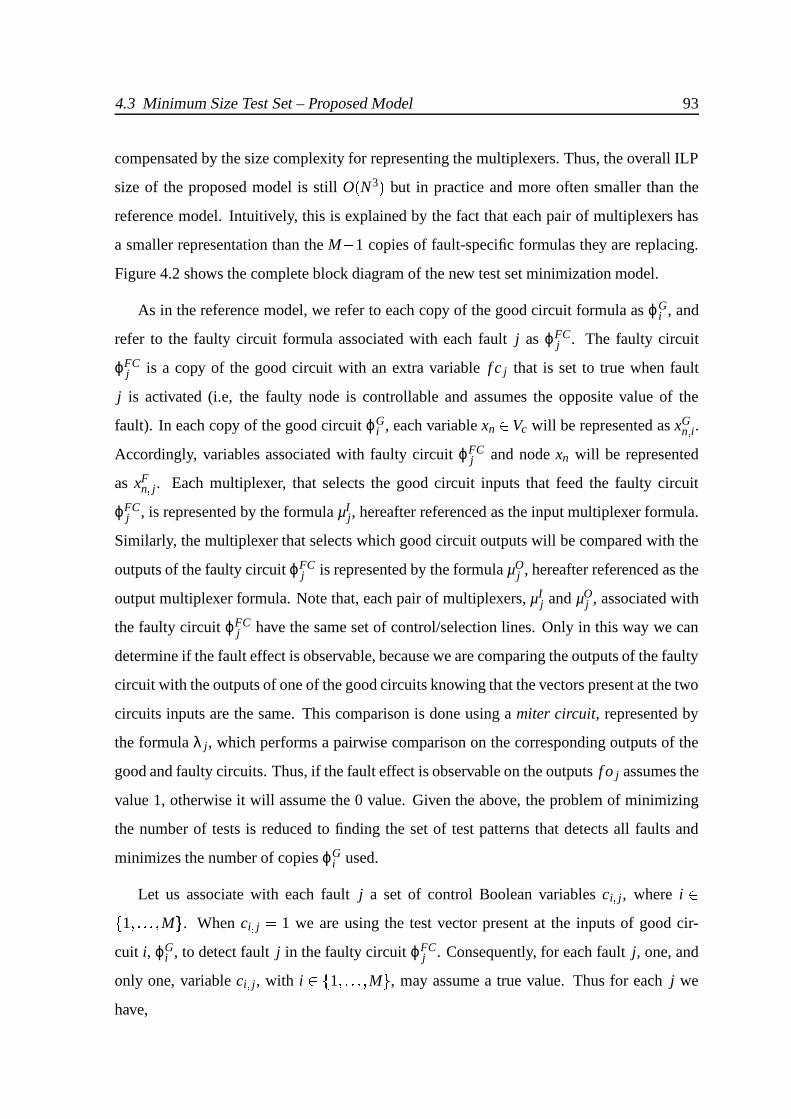
4.3 Minimum Size Test Set – Proposed Model 93
compensated by the size complexity for representing the multiplexers. Thus, the overall ILP
size of the proposed model is still O N3 but in practice and more often smaller than the
reference model. Intuitively, this is explained by the fact that each pair of multiplexers has
a smaller representation than the M 6 1 copies of fault-specific formulas they are replacing.
Figure 4.2 shows the complete block diagram of the new test set minimization model.
As in the reference model, we refer to each copy of the good circuit formula as ϕGi , and
refer to the faulty circuit formula associated with each fault j as ϕFCj . The faulty circuit
ϕFCj is a copy of the good circuit with an extra variable f c j that is set to true when fault
j is activated (i.e, the faulty node is controllable and assumes the opposite value of the
fault). In each copy of the good circuit ϕGi , each variable xn Vc will be represented as xG
n i.Accordingly, variables associated with faulty circuit ϕFC
j and node xn will be represented
as xFn j. Each multiplexer, that selects the good circuit inputs that feed the faulty circuit
ϕFCj , is represented by the formula µI
j, hereafter referenced as the input multiplexer formula.
Similarly, the multiplexer that selects which good circuit outputs will be compared with the
outputs of the faulty circuit ϕFCj is represented by the formula µO
j , hereafter referenced as the
output multiplexer formula. Note that, each pair of multiplexers, µIj and µO
j , associated with
the faulty circuit ϕFCj have the same set of control/selection lines. Only in this way we can
determine if the fault effect is observable, because we are comparing the outputs of the faulty
circuit with the outputs of one of the good circuits knowing that the vectors present at the two
circuits inputs are the same. This comparison is done using a miter circuit, represented by
the formula λ j, which performs a pairwise comparison on the corresponding outputs of the
good and faulty circuits. Thus, if the fault effect is observable on the outputs f o j assumes the
value 1, otherwise it will assume the 0 value. Given the above, the problem of minimizing
the number of tests is reduced to finding the set of test patterns that detects all faults and
minimizes the number of copies ϕGi used.
Let us associate with each fault j a set of control Boolean variables ci j, where i 1 M . When ci j 1 we are using the test vector present at the inputs of good cir-
cuit i, ϕGi , to detect fault j in the faulty circuit ϕFC
j . Consequently, for each fault j, one, and
only one, variable ci j, with i _ 1 M , may assume a true value. Thus for each j we
have,

94 4. Test Set Compaction Models
Input buses(width = #PI)
Output buses(width = #PO)
Control variables
PSfrag replacements
ϕG1
ϕGi
ϕGM
ϕFC1
ϕFCj
ϕFCM
µI1
µIj
µIM
µO1
µOj
µOM
c1 1c1 1
ci 1ci 1
cM 1cM 1
c1 jc1 j
ci jci j
cM jcM j
c1 Mc1 M
ci Mci M
cM McM M
X1 Xi XM Z1 Zi ZM
λ1
λ j
λM
f o1
f c1
f o j
f c j
f oM
f cM
Figure 4.2: Proposed formula organization for detecting all faults.
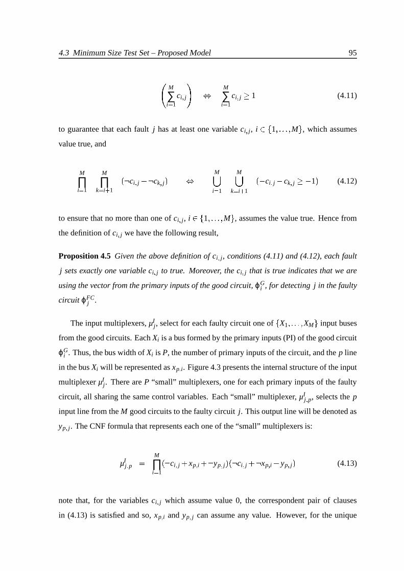
4.3 Minimum Size Test Set – Proposed Model 95
M
∑i 1
ci j M
∑i 1
ci j 1 (4.11)
to guarantee that each fault j has at least one variable ci j, i 1 M , which assumes
value true, and
M
∏i 1
M
∏k i 5 1
4: ci j _: ck j M,i 1
M,
k i 5 1
6 ci j 6 ck j 6 1 (4.12)
to ensure that no more than one of ci j, i 1 M , assumes the value true. Hence from
the definition of ci j we have the following result,
Proposition 4.5 Given the above definition of ci j, conditions (4.11) and (4.12), each fault
j sets exactly one variable ci j to true. Moreover, the ci j that is true indicates that we are
using the vector from the primary inputs of the good circuit, ϕGi , for detecting j in the faulty
circuit ϕFCj .
The input multiplexers, µIj, select for each faulty circuit one of X1 XM input buses
from the good circuits. Each Xi is a bus formed by the primary inputs (PI) of the good circuit
ϕGi . Thus, the bus width of Xi is P, the number of primary inputs of the circuit, and the p line
in the bus Xi will be represented as xp i. Figure 4.3 presents the internal structure of the input
multiplexer µIj. There are P “small” multiplexers, one for each primary inputs of the faulty
circuit, all sharing the same control variables. Each “small” multiplexer, µIj p, selects the p
input line from the M good circuits to the faulty circuit j. This output line will be denoted as
yp j. The CNF formula that represents each one of the “small” multiplexers is:
µIj p M
∏i 1
P: ci j xp i _: yp j 4: ci j _: xp i yp j (4.13)
note that, for the variables ci j which assume value 0, the correspondent pair of clauses
in (4.13) is satisfied and so, xp i and yp j can assume any value. However, for the unique

96 4. Test Set Compaction Models
PSfrag replacements x1 1x1 1xp 1
xp 1
xP 1
xP 1
x1 i
x1 i
xp i xp ixP i
xP ix1 M
x1 M
xp M
xp M
xPMxPM
y1 jy1 j
yp jyp jyP jyP j
µIj 1
µIj p
µIj P
µIj
c1 jc1 j
ci jci j
cM jcM j
X1
Xi
XM
Yj
Figure 4.3: Internal structure representation of an input multiplexer µIj.
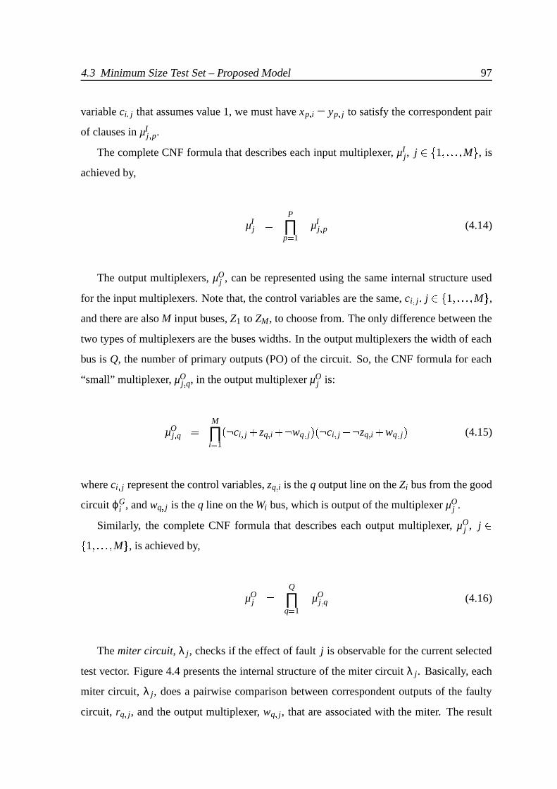
4.3 Minimum Size Test Set – Proposed Model 97
variable ci j that assumes value 1, we must have xp i yp j to satisfy the correspondent pair
of clauses in µIj p.
The complete CNF formula that describes each input multiplexer, µIj, j 1 M , is
achieved by,
µIj P
∏p 1
µIj p (4.14)
The output multiplexers, µOj , can be represented using the same internal structure used
for the input multiplexers. Note that, the control variables are the same, ci j j 1 M ,and there are also M input buses, Z1 to ZM, to choose from. The only difference between the
two types of multiplexers are the buses widths. In the output multiplexers the width of each
bus is Q, the number of primary outputs (PO) of the circuit. So, the CNF formula for each
“small” multiplexer, µOj q, in the output multiplexer µO
j is:
µOj q M
∏i 1
4: ci j zq i _: wq j P: ci j _: zq i wq j (4.15)
where ci j represent the control variables, zq i is the q output line on the Zi bus from the good
circuit ϕGi , and wq j is the q line on the Wi bus, which is output of the multiplexer µO
j .
Similarly, the complete CNF formula that describes each output multiplexer, µOj , j 1 M , is achieved by,
µOj Q
∏q 1
µOj q (4.16)
The miter circuit, λ j, checks if the effect of fault j is observable for the current selected
test vector. Figure 4.4 presents the internal structure of the miter circuit λ j. Basically, each
miter circuit, λ j, does a pairwise comparison between correspondent outputs of the faulty
circuit, rq j, and the output multiplexer, wq j, that are associated with the miter. The result
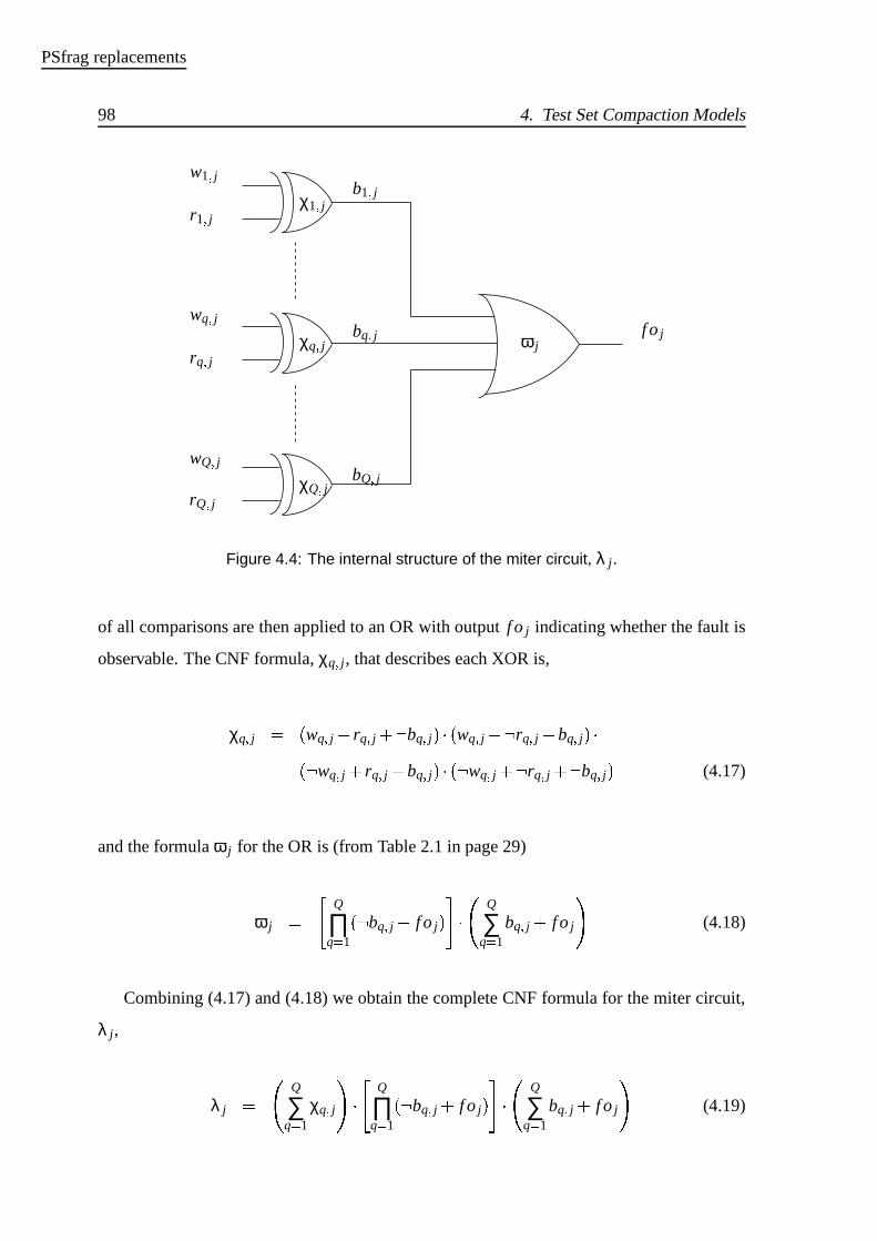
98 4. Test Set Compaction Models
PSfrag replacements
w1 jr1 jwq jrq jwQ jrQ j
b1 jbq jbQ j
χ1 jχq jχQ j
ω jf o j
Figure 4.4: The internal structure of the miter circuit, λ j.
of all comparisons are then applied to an OR with output f o j indicating whether the fault is
observable. The CNF formula, χq j, that describes each XOR is,
χq j wq j rq j _: bq j ¥ wq j : rq j bq j 4: wq j rq j bq j ¥P: wq j _: rq j _: bq j (4.17)
and the formula ω j for the OR is (from Table 2.1 in page 29)
ω j Q
∏q 1
4: bq j f o j Q
∑q 1
bq j f o j (4.18)
Combining (4.17) and (4.18) we obtain the complete CNF formula for the miter circuit,
λ j,
λ j Q
∑q 1
χq j Q
∏q 1
4: bq j f o j Q
∑q 1
bq j f o j (4.19)

4.3 Minimum Size Test Set – Proposed Model 99
To determine whether the faulty node is controllable from the primary inputs, i.e. whether
the fault is activated, we associate a Boolean variable f c j to each faulty circuit. Therefore,
the value of f c j depends on the value of the faulty node (xFCn j ) and the stuck-at value of the
fault. Thus, f c j must satisfy one of the following constraints:
λ j ! P: f c j xFCn j f c j : xFC
n j for fault xFCn j stuck-at-0 f c j xFC
n j 4: f c j : xFCn j for fault xFC
n j stuck-at-1(4.20)
Let us associate a Boolean variable vi with each good circuit formula ϕGi which assumes
value true whenever the primary inputs of the circuit formula i are used to detect any fault.
Moreover, each vi can be determined by all the multiplexers control variables that are asso-
ciated with each good circuit formula, ci j with j 1 M . Note that, if one of these
control variables is assigned value 1 we are using the inputs of ϕGi to detect fault j and then
vi must be true. Therefore, vi is obtained using an OR function,
vi OR ci 1 é ci j ci M (4.21)
which leads to the following constraint for all i 1 M , M
∏j 1
4: ci j vi M
∑j 1
ci j vi (4.22)
Observe that the variables vi are similar to the variables ui in the reference model, as both
indicate whether replica i of the good circuit is used to detect any target fault.
Finding the minimum size test set for irredundant combinational circuits implies that each
fault is controllable and observable. Therefore, we must assure that the following clauses
hold true,
M
∏j 1
f c j f o j
(4.23)

100 4. Test Set Compaction Models
# Clauses # Formulas
Circuit formula ϕG 34
Faulty circuit formula ϕFC 34
Fault detection (4.19) (4.20) 34
Detection requirement (4.23) 2 " 34 68
Control variables (4.11) (4.12) 34 " 1 f 34 « 332
19108
Input multiplexers (4.13) (4.14) 34 " 5 " 64 10880
Output multiplexers (4.15) (4.16) 34 " 2 " 64 4352
Usage of replica i (4.22) 34 " 34 1 1190
Cost function (4.24) 1
Table 4.3: Upper bounds using the new formulation model for the C17 benchmark circuit.
Finally, we must define the cost function that we want to minimize. Clearly, this cost
function should minimize the number of good circuits (which implies the number of vectors)
used for detecting all the faults, and so we get,
minM
∑i 1
vi (4.24)
The M replicas of the good circuit and the M representations of the faulty circuits with
the constraints represented by (4.11) through (4.24), capture the problem of computing min-
imum size test sets for irredundant circuits, using a linear number of circuit representations.
Table 4.3 summarizes the data associated with the new ILP formulation for the C17 bench-
mark circuit. Remember that, this benchmark circuit has 34 non-collapsed faults, 5 primary
inputs and 2 primary outputs.
Proposition 4.6 The size of the ILP for the minimum test set problem (described above) is
O M 12 M M 6 1 O N3 .
Proof. According to the structure of the model presented in Figure 4.2 we can associate

4.3 Minimum Size Test Set – Proposed Model 101
for each of the M copies of the good circuit formula, one faulty circuit formula, one set of
control variables, two multiplexers and one miter. For circuits with bounded fanin gates2,
each copy of the good and faulty circuits have representation size O N . The formulas
for each input and output multiplexer have its size bounded by O M PI and O M PO ,respectively. All the formulas for the usage of replicas and fault detection have size O M2 and O M PO , respectively, and all the detection requirement formulas have size O M . The
control variables formulas for each fault have size O 12 M M 6 1 . Since M O N , then
the size of the proposed ILP model becomes O N3 .We should note that, even though both models (reference and proposed) have size com-
plexity O N3 , the model described in this section exhibits in general a size smaller than the
reference model. Table 4.4 shows the estimated value of the number of clauses in the refer-
ence model and in the new model for the IWLS [IWLS 89] and for ISCAS’85 [Brglez 85]
benchmark circuits. The estimated values were determined considering that N is the total
number of nodes in each circuit, PI and PO are the number of primary inputs and outputs,
respectively, and M is the number of all the possible stuck-at faults in the circuit (no fault
collapsing was performed). For the ILP representation of the good and faulty circuits, and as
motivated below, we consider an average of 3 5 clauses for each node. Note, that a 2-input
basic gate uses 3 clauses, an XOR uses 4 clauses and a BUFFER or INVERTER just uses 2
clauses. We also consider for this estimate that the fault-specific representation (ϕFSi j in the
reference model) and the faulty circuit representation (ϕFCj in the proposed model) have the
same size, which may not necessarily be true. Note that, due to space reasons, the number
of literals for each model was omitted from the table, but they can be easily estimated by
determining the average number of literals per clause in each model (about 2.4 literals per
clause).
From these results we can conclude that the proposed model presents a size reduction in
the ILP formulation up to 47.85%, with an average value of 32%. This size reduction results
form the fact that for common circuits we have PI ¬ N and PO ¬ N. Therefore, the total
size of the multiplexers in the proposed model is significantly smaller than the size of the
2Circuits in which any gate in the circuit have at most k inputs.

102 4. Test Set Compaction Models
M ! M 6 1 extra faulty-specific circuits used in the reference model. In Section 4.3.3 we
will consider some practical considerations to further reduce the size of the proposed model.
4.3.2 Arbitrary Combinational Circuits
In this section we extend the previous model to identify a minimum test set that detects
all detectable faults in a given combinational circuit. As noted before, this problem is quite
similar to the one presented in the previous section, with the added difficulty that some faults
are now redundant.
The simple solution used in the reference model, will be followed. We will introduce
additional variables and modify some of the constraints of the previous section to support
circuits with redundant faults. First, let us define a variable r j, with j 1 M , that is
true when fault j is declared redundant. Given that some faults are indeed redundant, because
they are not observable and/or controllable, (4.23) must be modified to capture this fact:
M
∏j 1
f c j r j f o j r j
(4.25)
This constraint requires that each fault j is either detectable ( f c j 1 and f o j 1), in the
faulty circuit ϕFCj , or otherwise it must be declared redundant (r j 1). The next step is to
modify the cost function to minimize so it penalizes the existence of redundant faults,
min M
∑i 1
vi M M
∑j 1
r j (4.26)
This cost function is identical to the cost function (4.10) presented on the reference model
in Section 4.2.2. Giving a sufficiently large weight to the r j variables, bigger than the sum
of all vi, we are penalizing the existence of redundant faults. Hence, the minimum value of
the cost function is achieved only when all faults declared as redundant cannot actually be
detected. The ILP formulation for this problem using the proposed model is summarized in
Table 4.5.

4.3 Minimum Size Test Set – Proposed Model 103
Benchmark Nodes Inputs Outputs Faults Ref. Model New Model Reduction
circuit # N % # PI % # PO % # M % (# of clauses) (# of clauses) (%)
9symml 167 9 1 752 3.38E+08 2.27E+08 32.80
alu4 606 14 8 2704 1.57E+10 1.05E+10 33.06
cht 292 47 36 820 7.46E+08 5.10E+08 31.67
cm138a 40 6 8 124 2.43E+06 2.03E+06 16.65
cm150a 84 21 1 232 1.72E+07 8.99E+06 47.84
cm163a 75 16 5 220 1.39E+07 8.66E+06 37.81
cmb 74 16 4 248 1.74E+07 1.14E+07 34.42
comp 140 32 3 480 1.22E+08 7.52E+07 38.27
comp16 259 35 3 960 8.74E+08 5.28E+08 39.65
cordic 99 23 2 342 4.39E+07 2.72E+07 38.07
cu 76 14 11 254 1.90E+07 1.51E+07 20.82
dalu 918 75 16 3742 4.63E+10 2.99E+10 35.48
majority 18 5 1 54 2.13E+05 1.34E+05 37.20
misex1 67 8 7 220 1.23E+07 8.55E+06 30.33
misex2 127 25 18 414 8.43E+07 6.59E+07 21.75
misex3 561 14 14 2574 1.32E+10 9.37E+09 29.13
mux 69 21 1 202 1.09E+07 6.20E+06 43.25
pcle 104 19 9 328 4.26E+07 2.87E+07 32.66
pcler8 138 27 17 396 8.33E+07 5.85E+07 29.79
term1 199 34 10 704 3.69E+08 2.44E+08 33.98
too large 275 38 3 1132 1.29E+09 8.51E+08 34.06
unreg 155 36 16 448 1.20E+08 8.23E+07 31.53
C17 13 5 2 34 6.57E+04 5.02E+04 23.71
C432 203 36 7 864 5.65E+08 4.14E+08 26.83
C499 275 41 32 998 1.04E+09 8.03E+08 22.42
C880 469 60 26 1760 5.36E+09 3.67E+09 31.65
C1355 619 41 32 2710 1.65E+10 1.22E+10 25.91
C1908 938 33 25 3816 4.87E+10 3.13E+10 35.72
C2670 1566 233 140 5340 1.67E+11 1.17E+11 29.71
C3540 1741 50 22 7080 3.09E+11 1.90E+11 38.48
C5315 2608 178 123 10630 1.07E+12 7.38E+11 30.74
C6288 2480 32 32 12576 1.38E+12 1.04E+12 24.82
C7552 3827 207 108 15104 3.13E+12 1.99E+12 36.39
Table 4.4: Estimated ILP size for some benchmark circuits.
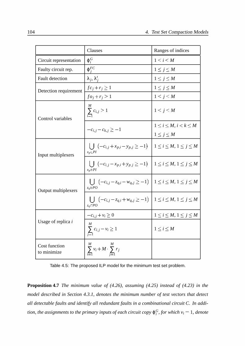
104 4. Test Set Compaction Models
Clauses Ranges of indices
Circuit representation ϕGi 1 3 i 3 M
Faulty circuit rep. ϕFCj 1 3 j 3 M
Fault detection λ j, λ j 1 3 j 3 M
Detection requirementf c j r j
1 1 3 j 3 M
f o j r j
1 1 3 j 3 M
Control variables
M
∑i 1
ci j 1 1 3 j 3 M
6 ci j 6 ck j 6 11 3 i 3 M, i k 3 M
1 3 j 3 M
Input multiplexers
,xp . PI
§ 6 ci j xp i 6 yp j 6 1 ¨ 1 3 i 3 M, 1 3 j 3 M,xp . PI
§ 6 ci j 6 xp i yp j 6 1 ¨ 1 3 i 3 M, 1 3 j 3 M
Output multiplexers
,zq . PO
§ 6 ci j zq i 6 wq j 6 1 ¨ 1 3 i 3 M, 1 3 j 3 M,zq . PO
§ 6 ci j 6 zq i wq j 6 1 ¨ 1 3 i 3 M, 1 3 j 3 M
Usage of replica i
6 ci j vi
0 1 3 i 3 M, 1 3 j 3 M
M
∑j 1
ci j vi
1 1 3 i 3 M
Cost functionto minimize
M
∑i 1
vi M M
∑j 1
r j
Table 4.5: The proposed ILP model for the minimum test set problem.
Proposition 4.7 The minimum value of (4.26), assuming (4.25) instead of (4.23) in the
model described in Section 4.3.1, denotes the minimum number of test vectors that detect
all detectable faults and identify all redundant faults in a combinational circuit C. In addi-
tion, the assignments to the primary inputs of each circuit copy ϕGi , for which vi 1, denote

4.3 Minimum Size Test Set – Proposed Model 105
a test pattern. Finally, each variable r j set to true indicates that fault j is redundant.
4.3.3 Practical Considerations and Other Improvements
In practice the size of the model can be reduced if we consider the techniques presented
for the reference model in Section 4.2.3, which can also be used in the new model. Therefore,
in practice we will remove the redundant faults from the fault set, apply fault dominance and
independence relationships, and use empirical upper bounds to reduce the size of the ILP
model. Table 4.3 shows an upper bound on the size of the ILP model for the C17 bench-
mark circuit considering all the of 34 stuck-at faults present in the circuit. But, considering
fault dominance relations the set of faults could be collapsed into 17 faults [Brglez 85]. So,
only 17 faulty circuit representations ϕFCj , need to be considered. Moreover, by running the
ATPG algorithm ATALANTA [Lee 93] only 4 test patterns are identified. Thus, only 4 circuit
representations are needed at most to detected all faults. Likewise, the number of all other
clauses used in the ILP formulation are also reduced once the range of i and j indices are
narrowed to 1 3 i 3 4 and 1 3 j 3 17, because we need at most 4 vectors and there are only
17 collapsed faults, respectively.
Two other type of improvements can be implemented in the model itself to further re-
duce the size of the resulting ILP. First, in each miter circuit we just need to compare the
outputs that are in the transitive fan-out of the fault (i.e. the outputs of the circuit in which
the fault effect could be observed). Therefore, in the output multiplexers it is not necessary
to multiplex the outputs that will not be used by the miter. This will reduce the bus width
of each output multiplexer to the number of primary outputs that are in the transitive fan-out
of the corresponding fault, which in general are significantly fewer than Q (the total number
of primary outputs). This improvement to the model can significantly reduce the number of
clauses in the fault detection formulas (by reducing the size of the miter circuits) and in the
output multiplexers. Second, the bus width on the input multiplexers can also be reduced.
Each input multiplexer does not need to multiplex all the primary inputs of the circuit, but
only those that can be involved in the fault activation and the fault propagation to the outputs
(primary inputs in the transitive fan-in of the primary outputs that are in the transitive fan-out
of the faulty node). This improvement to the model will reduce the number clauses in the

106 4. Test Set Compaction Models
input multiplexers.
Moreover, the size of the input multiplexers can be further reduced (by reducing its bus
width), if we directly multiplex some internal nodes of the circuit instead of the primary
inputs. The nodes selected for multiplexing should form a cut, with the minimum number of
nodes, in the sub-circuit composed by the nodes of the immediate fanin cone of influence of
the faulty node. Naturally, the total number of selected nodes for multiplexing is less or equal
than the number of primary inputs involved in the fault activation and propagation. Observe
that by selecting internal nodes for multiplexing we are also reducing the representation size
of each faulty circuit, because the nodes in the transitive fanin of the selected nodes do not
need to be in the faulty circuit representation anymore.
4.4 Maximum Test Set Compaction
As illustrated by Table 4.4, the previous models for computing the minimum size test
set for larger circuits are (currently) impractical. Therefore, in this section we will consider
a practical alternative approach for computing minimized test sets. First, we review the set
covering model for test set compaction. Then, we use a highly effective algorithm for the
unate covering problem [Coudert 96] and evaluate the application of the model in the sim-
plification of test sets. Moreover, we study the relationship between the application of fault
simulation and the ability of reducing the test set size. Experimental evidence, obtained on a
large number of benchmark circuits, clearly indicates that the utilization of fault simulation
in general reduces the ability for computing smaller test sets.
4.4.1 Set Covering Model for Test Compaction
Let F f1 fm be the set of stuck-at faults of a combinational circuit C, and let
T t1 tn be a pre-computed test set. Furthermore, let the faults detected by test pattern
t j be F t j f j1 f jk . Consequently, the objective of the test set compaction problem
is to find a set of test patterns U T , such that,

4.4 Maximum Test Set Compaction 107
F ,t j . U
F t j (4.27)
and such that the size of U is minimum. This problem can naturally be mapped into an
instance of the set covering problem. Indeed, define a matrix D where di j 1 provided test
pattern t j detects fault fi. Further, define a vector x of Boolean variables, with size 1 " n ,such that x j 1 provided test pattern t j is selected for inclusion in U . Consequently, our goal
is to solve the following integer optimization problem,
minimize ∑x j
subject to D x 1 (4.28)
x j 0 1 j 7 1 ö n which can also be viewed as an instance of the set covering (or unate covering) problem.
This model was first described in [Hochbaum 96] and some results were obtained with a
set covering algorithm based on linear programming relaxations. Nevertheless, other more
efficient set covering algorithms can be used [Coudert 96], which allow for larger test sets
to be considered. This solution in turn allows considering different test pattern generation
strategies which, in a preliminary phase, may generate a larger number of test patterns that
are later minimized with a set covering algorithm.
It should be noted that, only in the case the test set contains all possible input patterns then
the solution of (4.28) is guaranteed to obtain the minimum size test set for the given circuit.
In practice, the test set that is considered is provided by an ATPG tool, and hence denotes a
small subset of the set of all test patterns. However, as we will see, the experimental results
obtained with these reduced subsets produce satisfactory results when compared other test
set compaction tools.

108 4. Test Set Compaction Models
t1 t2 t3 t4
f1 1 0 0 1
f2 1 1 0 0
f3 0 0 1 1
f4 0 1 0 1
f5 1 0 1 0
Table 4.6: Covering table for a set of faults.
An Example
As an application example of the model presented in the previous section, let us con-
sider a combinational circuit with fault set f1 f2 f3 f4 f5 such that the set of test patterns t1 t2 t3 t4 detects all faults. Let us assume further that the relation between test patterns
and detected faults is as shown in Table 4.6, where an entry i j with value 1 indicates that
test pattern t j detects fault fi, and an entry with value 0 indicates that the fault is not detected
with t j. Using this information, the resulting covering problem can be formulated as follows:
minimize x1 x2 x3 x4 (4.29)
subject to the constraints, *®®®®®®®®®+
1 0 0 1
1 1 0 0
0 0 1 1
0 1 0 1
1 0 1 0
3°¯¯¯¯¯¯¯¯¯5 *®®®®®®+
x1
x2
x3
x4
3 ¯¯¯¯¯¯5 *®®®®®®+
1
1
1
1
3 ¯¯¯¯¯¯5 (4.30)
where each xi, 1 3 i 3 4, is a Boolean variable.
The minimum solution to this covering problem is x1 1 and x4 1, which indicates
that t1 and t4 can be selected as a reduced set of test patterns for detecting all faults in the

4.4 Maximum Test Set Compaction 109
circuit.
4.4.2 Experimental Results
The model described in the previous section has been applied to test sets computed by
ATALANTA [Lee 93], under different operating conditions, and by COMPACTEST [Pomeranz 93b].
The unate covering algorithm, scherzo [Coudert 96], has been applied to the different
test sets, with the objective of minimizing those test sets. The experimental results are
shown in Table 4.7 and in Table 4.8, respectively for the IWLS [IWLS 89] and for the IS-
CAS’85 [Brglez 85] benchmark circuits. In these tables, FS indicates the utilization of fault
simulation and CPT denotes the application of test compaction using simple dominance re-
lations on the test vectors. NoFS indicates that fault simulation is not applied, which means
that all faults were targeted. Note that ATALANTA computes test patterns with don’t cares,
which enhance dominance relations between test patterns. However, before applying the
unate covering algorithm, the test set compaction tool (MTSC) assigns random 0 5 1 values to
the don’t care bits, in order to increase the number of faults detected by each pattern. We
also observed that the simple dominance-based test compaction is very ineffective when-
ever fault simulation is applied during test generation. Thus, the experimental results from
FS+CPT are identical to the FS+NoCPT and, for simplicity, they are omitted form the tables.
For each experiment the total number of test patterns (#T) is shown, either obtained by the
ATALANTA tool (Atalanta), COMPACTEST tool (Ctest), or after applying the test set compaction
tool (MTSC) that runsscherzo. The CPU time allowed for scherzo was 4,000 seconds on a
SUN Sparc Ultra I/170 workstation with 384 Meg. of physical memory. Table entries with
‘—’ indicate that the CPU time was exceeded.
As can be concluded from the tables of results, test set compaction can in general yield
significant savings in the number of test patterns, even when fault simulation is applied.
Moreover, by not applying fault simulation, and thus by having a significantly larger initial
test set, the test set compaction procedure is able, in the vast majority of cases, to com-
pute test sets smaller than those obtained with fault simulation. Nevertheless, for the larger
circuits, the non-utilization of fault simulation yields a very large number of test patterns,
which the set covering algorithm may then be unable to simplify. One solution to overcome
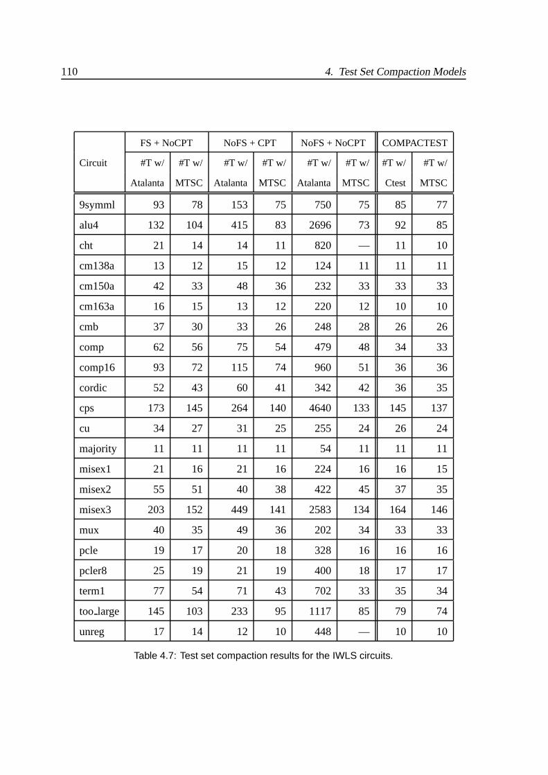
110 4. Test Set Compaction Models
FS + NoCPT NoFS + CPT NoFS + NoCPT COMPACTEST
Circuit #T w/ #T w/ #T w/ #T w/ #T w/ #T w/ #T w/ #T w/
Atalanta MTSC Atalanta MTSC Atalanta MTSC Ctest MTSC
9symml 93 78 153 75 750 75 85 77
alu4 132 104 415 83 2696 73 92 85
cht 21 14 14 11 820 — 11 10
cm138a 13 12 15 12 124 11 11 11
cm150a 42 33 48 36 232 33 33 33
cm163a 16 15 13 12 220 12 10 10
cmb 37 30 33 26 248 28 26 26
comp 62 56 75 54 479 48 34 33
comp16 93 72 115 74 960 51 36 36
cordic 52 43 60 41 342 42 36 35
cps 173 145 264 140 4640 133 145 137
cu 34 27 31 25 255 24 26 24
majority 11 11 11 11 54 11 11 11
misex1 21 16 21 16 224 16 16 15
misex2 55 51 40 38 422 45 37 35
misex3 203 152 449 141 2583 134 164 146
mux 40 35 49 36 202 34 33 33
pcle 19 17 20 18 328 16 16 16
pcler8 25 19 21 19 400 18 17 17
term1 77 54 71 43 702 33 35 34
too large 145 103 233 95 1117 85 79 74
unreg 17 14 12 10 448 — 10 10
Table 4.7: Test set compaction results for the IWLS circuits.

4.4 Maximum Test Set Compaction 111
FS + NoCPT NoFS + CPT NoFS + NoCPT COMPACTEST
Circuit #T w/ #T w/ #T w/ #T w/ #T w/ #T w/ #T w/ #T w/
Atlanta MTSC Atalanta MTSC Atalanta MTSC Ctest MTSC
C432 78 60 184 44 520 41 50 44
C499 93 58 276 57 750 52 63 56
C880 69 50 116 44 942 — 30 29
C1355 131 93 523 87 1566 84 96 85
C1908 179 128 520 116 1870 — 137 122
C2670 159 111 300 106 2621 — 69 67
C3540 211 145 137 126 3291 — 113 110
C5315 1781 109 619 — 5291 — 55 55
C6288 36 24 714 — 7114 — 16 16
C7552 288 215 572 149 7292 — 87 86
Table 4.8: Test set compaction results for the ISCAS’85 circuits.
this problem is to compact test patterns by using dominance relations (columns NoFS+CPT
in the tables). In this case, the set covering algorithm is able to optimally solve a larger
number of problem instances. Nevertheless, in the same example the number of test patterns
may still be too large for the set covering algorithm to handle. One additional simplification
technique that was implemented consists in the partition of the test set into k subsets and
simplifying each subset separately. Afterwards, the process is repeated for a selected pair of
subsets. The process is repeated until the minimum (for the given set of vectors) is reached
or a satisfactory reduced test set is obtained.
As one final remark, we should note that the improvements obtained with the test set
compaction procedure also result from the ATPG tool computing test sets that are signifi-
cantly larger than the optimum. Nevertheless, the set covering procedure of Section 4.4.1
can be applied to test sets computed by any ATPG tool (e.g. COMPACTEST [Pomeranz 93b] or
MinTest [Hamzaoglu 98]) whenever these test sets are known not to be optimum. As showed
in Table 4.7 and Table 4.8 the test set compaction tool (MSTC) is able to further reduce, in

112 4. Test Set Compaction Models
same cases, the number of test vectors generated by the COMPACTEST tool.
4.5 Conclusions
In this chapter we described CNF formulations for the identification of test patterns and
showed how these formulations can be used for constructing integer linear programs (ILP)
for solving optimization problems in testing, in particular the minimum test set problem.
A reference model for the minimum test set problem was described in which the size of
the ILPs is in the worst-case polynomial in the number of circuit nodes. This contrasts with
other solutions [Matsunaga 93], which require worst-case exponential-size representations.
We proposed a new model for the minimum size test set problem which is also worst-case
polynomial in the number of circuit nodes. Nevertheless, we showed that, for benchmark
circuits, the proposed model can reduce the size of the ILPs up to 47.85%. We also pre-
sented some techniques to reduce further the size of the new model. Besides their theoretical
interest, the model can only be used in small-size circuits for validating new heuristics for
test set compaction, e.g. to confirm how close a test set solution, computed heuristically, is
far from the optimum solution. However, for most circuits the proposed ILP formulation is
still too complex to be solved with existing tools.
Therefore, we decided, in the scope of this work, not to implement the new model but,
to describe and evaluate an alternative approximate algorithm for test set compaction. The
algorithm, based on set covering, can be used as a post-processing tool to further compact
test sets obtained with ATPG algorithms. Experimental evidence indicates that in general ad-
ditional test set compaction can be achieved. Moreover, by augmenting the size of the initial
test set, e.g. by not using fault simulation and targeting all faults, we were able to compute
test sets that are in general smaller than those obtained when fault simulation is used. Hence,
whenever the main objective is test set compaction one may consider utilizing highly ef-
ficient ATPG algorithms, targeting all faults (i.e. no fault simulation) and applying the set
covering algorithm for test set minimization. Despite this interesting result, set covering is
an NP-hard problem and consequently existing algorithms may be unable to handle large
test sets. For this problem we proposed different techniques, including precompaction of test

4.5 Conclusions 113
sets based on dominance relations and test set partitioning. In general, the results obtained
with the developed MTSC compaction tool are satisfactory and showed, in particular, that
compacted test sets obtained heuristic with approaches (eg. COMPACTEST [Pomeranz 93b])
can be further reduced.

114

Chapter 5
Minimum Size Test Patterns
Contents
5.1 Introduction
5.2 Test Generation With Unspecified Variable Assignments
5.2.1 Modeling Unspecified Variable Assignments
5.2.2 Test Pattern Generation with Unspecified Input Assignments
5.3 Computing Minimum Size Test Patterns
5.3.1 The Complete Optimization Model
5.4 Limitations of the Model
5.5 Experimental Results
5.6 Conclusions
115

116 5. Minimum Size Test Patterns
5.1 Introduction 117
5.1 Introduction
As seen in Chapter 2, automatic test pattern generation (ATPG) for stuck-at faults in
combinational circuits is now a mature field, with an impressive number of highly effective
models and algorithms [Chakradhar 93, Cox 94, Fujiwara 83, Giraldi 91, Goel 81, Silva 94,
Kirkland 87, Kunz 92, Larrabee 92, Lee 93, Schulz 89, Stephan 96, Teramoto 93]. Further-
more, besides being effective at detecting the target faults, recent ATPG tools have targeted
the heuristic minimization (i.e. compaction) of the total number of test patterns required
for detecting all faults in a circuit [Chakrabarty 97, Pomeranz 93b, Niermann 91, Schulz 89,
Hellebrand 95b, Hamzaoglu 98]. The optimization of test sets was discussed in the previ-
ous chapter, where we proposed different deterministic models for the problem. In general,
the degree of test pattern compaction is expected to be related to the number of unspeci-
fied input assignments in each test pattern. In addition, for applications where testing time
and fault coverage requirements can only be achieved with dedicated Finite-State Machine
(FSM) controllers, the computation of test patterns with a large number of unspecified input
assignments may allow for significantly smaller synthesized FSMs. Indeed, if the test set is
used as input to a logic synthesis tool with the purpose of synthesizing BIST logic, then by
maximizing the number of unspecified input assignments, i.e. by maximizing the don’t care
set of each test pattern, the logic synthesis tool is in general able to yield smaller synthesized
logic. Thus, the maximization of the don’t care set of each test pattern, or conversely, the
computation of test patterns of minimum-size, can have significant practical advantages.
Nevertheless, until the work of P. Flores et al. [Flores 98b], there existed no known model
or algorithm for computing test patterns for which the number of unspecified primary input
assignments is maximized. In this chapter we will describe in detail the model proposed. We
start by formalizing the notion of test pattern minimization. We then explain the model for
test pattern generation in the presence of unspecified input assignments, based on proposi-
tional satisfiability (SAT). Next, we derive an integer linear programming (ILP) model for
maximizing the number of unspecified primary input assignments. Finally, we provide a set
of results that justify using the proposed model in medium-size combinational circuits and
describe an ATPG methodology, which can incorporate the proposed model and support-
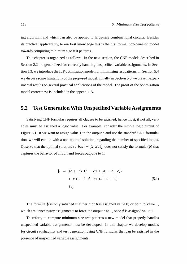
118 5. Minimum Size Test Patterns
ing algorithm and which can also be applied to large-size combinational circuits. Besides
its practical applicability, to our best knowledge this is the first formal non-heuristic model
towards computing minimum size test patterns.
This chapter is organized as follows. In the next section, the CNF models described in
Section 2.2 are generalized for correctly handling unspecified variable assignments. In Sec-
tion 5.3, we introduce the ILP optimization model for minimizing test patterns. In Section 5.4
we discuss some limitations of the proposed model. Finally in Section 5.5 we present exper-
imental results on several practical applications of the model. The proof of the optimization
model correctness is included in the appendix A.
5.2 Test Generation With Unspecified Variable Assignments
Satisfying CNF formulas requires all clauses to be satisfied, hence most, if not all, vari-
ables must be assigned a logic value. For example, consider the simple logic circuit of
Figure 5.1. If we want to assign value 1 to the output e and use the standard CNF formula-
tion, we will end up with a non-optimal solution, regarding the number of specified inputs.
Observe that the optimal solution, a b d X X 1 , does not satisfy the formula (ϕ) that
captures the behavior of circuit and forces output e to 1:
ϕ a _: c b _: c ¥4: a : b c P: c e 4: d e d c : e (5.1) e The formula ϕ is only satisfied if either a or b is assigned value 0, or both to value 1,
which are unnecessary assignments to force the output e to 1, once d is assigned value 1.
Therefore, to compute minimum size test patterns a new model that properly handles
unspecified variable assignments must be developed. In this chapter we develop models
for circuit satisfiability and test generation using CNF formulas that can be satisfied in the
presence of unspecified variable assignments.

5.2 Test Generation With Unspecified Variable Assignments 119
a
b
de
c
Figure 5.1: Simple circuit for which we want to force output e 1.
5.2.1 Modeling Unspecified Variable Assignments
Given a circuit and its associated CNF formula or a fault f and its associated fault de-
tection formula, the existence of unspecified assignments implies that each of the original
circuit variables can now be assigned a value in the set 0 1 X . In this situation an assign-
ment x X indicates that x is unspecified, or that the value assumed by x is an unspecified
assignment1. This signifies that an assignment A is now allowed to leave variables unspeci-
fied.
To decide CNF formula satisfiability, in the presence of unspecified variables, a new set of
variables must be created. This basically consists of duplicating the number of Boolean vari-
ables, which is a common solution for capturing unspecified assignments [Pizzuti 96]. Since
only 3M assignments need to be considered for M variables, the actually minimum number
of Boolean variables required is ± log2 3M ² . However, considering instead 2M variables
greatly simplifies the proposed model. As a result, we propose to represent each Boolean
variable x with two new variables x0 and x1 having the interpretation indicated in Table 5.1.
For this interpretation, x X indicates that x is unspecified. The simultaneous assignment of
variables x0 and x1 to 1 is not allowed, requiring the inclusion of the following constraint in
the resulting CNF formula,
ϕinv x 4: x1 : x0 (5.2)
1Note that x ³ ´ 0 $ 1 µ indicates that x is specified, or that the value assumed by x is a specified assignment.

120 5. Minimum Size Test Patterns
x x1 x0 0 0 1 1 1 0 X 0 0
Table 5.1: Interpretation of the new variables modeling unspecified assignments.
w1 w2 x w11 w0
1 w1
2 w02 x1 x0 0 0 0 0 0 0 0 0 0 1 0 1 0 0 1 0 0 0 0 1 0 0 0 1 0 1 0 1 0 1 0 1 1 0 0 1 1 0 0 0 0 0 1 0 0 1 0 1 1 0 1 0 1 0
Table 5.2: Truth table of a generalized AND (UAND) using the new variables.
for each node x VC, where VC represents the set of nodes in the circuit (or problem vari-
ables).
In addition, for each basic gate type we need to define the corresponding CNF formula,
considering that each gate input and output must now be replaced by two variables. Let us
consider for example a 2-input AND gate, which will now be denoted by the generalized
form x0 x1 UAND w01 w1
1 w21 w1
2 . Table 5.2 presents the truth table of this gate using
the new input and output variables. Note that the simultaneous assignment of any pair of
variables to 1 is prevented by (5.2), thus we just need to relate the remaining assignments.
In this table, it can easily be observed that the output variable x0 assumes value 1 provided
at least one input variable w01 or w0
2 assumes value 1. Hence, x0 can be expressed as the OR

5.2 Test Generation With Unspecified Variable Assignments 121
x0
x1
w1
w2
x
w02
w01
w11
w12
Figure 5.2: Abstract view of a generalized 2-inputs AND gate (UAND).
of the input variables w01 and w0
2. Identically, the output variable x1 can only assume value 1
whenever all input variables w11 and w1
2 assume value 1. Hence, x1 can be expressed as the
AND of the input variables w11 and w1
2. Figure 5.2 provides an abstract view of this general-
ized 2-input AND gate using a binary OR and AND gate. Therefore, the CNF formulas for
the generalized AND are,
ϕu x0 P: w01 x0 ¥P: w0
2 x0 w01 w0
2 _: x0 (5.3)
ϕu x1 w11 _: x1 ¥ w1
2 : x1 4: w11 _: w1
2 x1 Observe that in addition (5.2) should be applied to each node.
Let us consider now a generalized AND gate with j-inputs, denoted by the general form x0 x1 UAND w01 w1
1 w0j w1
j . We still can conclude that the output variable x0 as-
sumes value 1 provided at least one input variable w0j is assigned value 1, and that the output
variable x1 can only assume value 1 if all inputs variables w1j assume value 1. Thus, we can
say that
x0 OR w01 w0
j
(5.4)
x1 AND w11 w1
j
122 5. Minimum Size Test Patterns
Considering the two CNF formulas, in Table 2.2, that describe the simple logic gates OR
and AND,
ϕu x0 j
∏i 1
4: w0i x0 j
∑i 1
w0i _: x0
(5.5)
ϕu x1 j
∏i 1
w1i : x1 j
∑i 1
: w1i x1
the CNF formula for a generic UAND gate with output x becomes
ϕu x ϕu x18 ϕu x0
8 ϕinv x (5.6)
which properly models unspecified assignments to the inputs and output of an AND gate.
Similar relations can be derived for the other simple gates. Consequently, the CNF for-
mulas for the simple gates given in Table 2.1 (see page 29) can be generalized by following
the same approach used for deriving (5.5). These generalized CNF formulas for the same
simple gates are given in Table 5.3. As a result, and as done in Section 2.2, we can now cre-
ate the CNF formula for the representation of the circuit, (ϕu), in which unspecified variable
assignments are allowed.
ϕu ,x . VC
ϕu x (5.7)
Figure 5.3 illustrates the outcome of applying an incompletely specified assignment to
the primary inputs of a simple circuit. As shown before the assignment d 1, with inputs a
and b unspecified, represents a sufficient condition for the assignment e 1 to be satisfied,
although this assignment does not satisfy the traditional CNF formula of the circuit, as given
in (5.1). Using the new variables that model unspecified assignments, the resulting CNF
formula of the circuit becomes

5.2 Test Generation With Unspecified Variable Assignments 123
c ¶¸· 0 ¹ 0 º¼» X
e ¶¸· 1 ¹ 0 º » 1
b ¶¸· 0 ¹ 0 º¼» X
d ¶¸· 1 ¹ 0 º¼» 1
a ¶¸· 0 ¹ 0 º¼» X
Figure 5.3: Example of unspecified assignments for a simple circuit.
ϕGu 4: a0 c0 ¥4: b0 c0 a0 b0 _: c0 a1 _: c1 ¥ b1 : c1 4: a1 _: b1 c1
(5.8) c0 _: e0 ¥ d0 _: e0 ¥4: c0 _: d0 e0 4: c1 e1 ¥P: d1 e1 ¥ c1 d1 _: e1 where the emphasized literals assume value 1 for the input assignments a b d X X 1 .Thus, all clauses are satisfied and consequently the whole CNF formula is satisfied.
5.2.2 Test Pattern Generation with Unspecified Input Assignments
We can now generalize the test pattern generation model described on Section 2.2 so that
unspecified variable assignments are allowed. Each circuit node x is still characterized by
three variables: xG denoting the value in the good circuit. This variable can be unspecified, and so
we use two new variables to characterize its value, xG 0 and xG 1, with the semantic
definition given earlier. xF denoting the value in the faulty circuit. This variable can also be unspecified, and
so we use two new variables to characterize its value, xF 0 and xF 1, with the semantic
definition given earlier.

124 5. Minimum Size Test Patterns
Gate type Gate function ϕu xi
AND
x0 OR w01 w0
j j
∏i 1
4: w0i x0 j
∑i 1
w0i _: x0
x1 AND w11 w1
j j
∏i 1
w1i _: x1 j
∑i 1
: w1i x1
NAND
x0 AND w11 w1
j j
∏i 1
w1i _: x0 j
∑i 1
: w1i x0
x1 OR w01 w0
j j
∏i 1
4: w0i x1 j
∑i 1
w0i _: x1
OR
x0 AND w01 w0
j j
∏i 1
w0i _: x0 j
∑i 1
: w0i x0
x1 OR w11 w1
j j
∏i 1
4: w1i x1 j
∑i 1
w1i _: x1
NOR
x0 OR w11 w1
j j
∏i 1
4: w1i x0 4 j
∑i 1
w1i _: x0
x1 AND w01 w0
j j
∏i 1
w0i _: x1 j
∑i 1
: w0i x1
NOTx0 BUFF w1
1 w1
1 _: x0 ¥4: w11 x0
x1 BUFF w01 w0
1 _: x1 ¥4: w01 x1
BUFFx0 BUFF w0
1 w0
1 _: x0 ¥4: w01 x0
x1 BUFF w11 w1
1 _: x1 ¥4: w11 x1
Table 5.3: Generalized CNF formulas for simple gates.

5.2 Test Generation With Unspecified Variable Assignments 125 xS denoting the sensitization status of each node. As we will justify below, the sensi-
tization status of each node needs not be unspecified, and so its value is always either
0 or 1.
The CNF formula that describes the good circuit, using the good variables (xG 0 and xG 1),
is obtained as described before on Section 2.2. However, to consider unspecified assignments
to the gates inputs and outputs, the generalized formulas presented in Table 5.3 must be used,
for each gate in the circuit.
For completely specified assignments, the CNF formulas used for computing the good
values and the faulty values for each gate are equal, because when the generated test pattern
is applied to the circuit the differences between the good and the faulty circuits results from
faults.
For incompletely specified test patterns the difference between the good and the faulty
circuit results from a fault and/or from the values assigned to unspecified inputs, during the
circuit test. To avoid blocking the fault propagation and make the fault undetectable, for some
realizations of don’t cares values, we prevent propagating a faulty value without knowing the
good value, which are the values using during test. Figure 5.4 shows a circuit (AND gate)
that exemplifies this situation. Note that the set of assignments for the inputs/outputs of
the good circuit and the faulty circuit are valid and will detect the fault stuck-at-1 in node
w1. The fault is activated (wG1 0 and wF
1 1) and its effect is observed in the output
(xG xF 1). If the test vector w1 w2 0 X is applied during circuit testing as 0 1 ,
the fault is observed and detected. But, if the circuit is tested with the test vector 0 0 , the
fault is not observed in the output, because its effect is blocked or masked by the assignment
w2 0.
Thus, we need to introduce an additional constraint for which an unspecified good value
implies an unspecified faulty value,
xG X ½0 xF X (5.9)
this way we guarantee that the good and faulty circuit are always “synchronized” and the
only difference between them are caused by the fault.

126 5. Minimum Size Test Patterns
PSfrag replacements
wG1 0
wG2 X
xG 0
wF1 1
wF2 1
xF 1
Good circuit Faulty circuit
(a) (b)
Figure 5.4: Node variables for (a) good and (b) faulty circuit when w1 is stuck-at-1.
Let us assume that the CNF formula for the faulty value of a node x with completely
specified assignments is given by,
ϕFx j
∏i 1
ωi (5.10)
Using the new generalized formulas for the gates (from Table 5.3), we will get a new set
of clauses ω i. Combining the restriction imposed by (5.9), the resulting CNF formula for the
faulty circuit, in the presence of incompletely specified assignments, is defined by,
ϕFu x 4: xF 0 xG 0 xG 1 4: xF 1 xG 0 xG 1 j
∏i 1
ω i _: xG 0 : xG 1 4: xF 0 xG 0 xG 1 4: xF 1 xG 0 xG 1 j
∏i 1
ω i : xG 0 ω i _: xG 1 (5.11)
Hence, the faulty value of a node x is computed by its original formula provided the good
value is specified (i.e., xG 0 xG 1 1). In contrast, if the good value is unspecified (i.e.,
xG 0 xG 1 0), then the faulty value is forced to also be unspecified.
Modeling unspecified assignments in test generation requires a detailed characterization
of the propagation conditions of the fault effect. Remember from Section 2.2 that the sen-
sitization variable of a node should assume value 1, if in that node we can differentiate the

5.2 Test Generation With Unspecified Variable Assignments 127
good and the faulty circuit, and a value of 0 if that is not possible. Hence, the sensitization
status xS of a node can only assume value 1 when both values of the node in the good and
faulty circuits are specified and assume different logic values. Moreover, this requirement
also causes the value of a node in the faulty circuit to be specified only when the value of that
node in the good circuit is also specified. These constraints indicate that propagation of the
fault effect to a node can only be guaranteed when the values in the good and faulty circuit
are specified for that node.
The relationship between the value of xS and the possible values of xG and xF is shown
in Table 5.4. The first four entries are similar to the model for completely specified assign-
ments, xS assumes value 1 if and only if xG and xF assume opposing logic values, provided
that both xG and xF are specified. The next three entries define the sensitization variable as 0
whenever the value in the faulty circuit is unspecified. The last two entries with a ‘ 6 ’ denote
invalid value assignments, for which the CNF formula for xS must assume value 0. Observe
that (5.9) prevents these combinations of values from occurring. The simplification of the
truth Table 5.4 yields the following CNF formula for the sensitization status of node x, xS:
ϕSu x xG 0 xF 0 _: xS ¥ xG 0 : xF 0 xS xG 1 xF 1 _: xS ¥ xG 1 : xF 1 xS (5.12)
The formulas for ϕSu x and for ϕF
u x are defined so that an unspecified good value imme-
diately implies an unspecified faulty value and xS 0. Thus, propagation of the error signal
is only permitted in the presence of properly specified values for the good circuit variables.
Otherwise, we could be propagating a false error condition, because it could became blocked
by some assignment of the unspecified inputs during the circuit testing.
Furthermore, we note that the remaining CNF formulas of Table 2.2, i.e. propagation
blocking conditions ϕB and fault detection requirements ϕR, remain unchanged, whereas
the fault activation conditions ϕA must be updated to the new set of variables. As a result,
the complete CNF formula for a given stem fault z stuck-at-v is summarized in Table 5.5.
Observe that in Table 5.5 we refer to ϕDu as the fault-detection formula in the presence of
unspecified variable assignments. Similarly, we can derive the CNF formula for a fanout-
branch fault.

128 5. Minimum Size Test Patterns
xG xF xS
0 0 0
0 1 1
1 0 1
1 1 0
X X 0
0 X 0
1 X 0
X 0 6X 1 6
Table 5.4: Truth table for the sensitization status.
5.3 Computing Minimum Size Test Patterns
In this section we develop the optimization model for computing minimum-size test pat-
terns. This optimization model is based on test pattern generation in the presence of incom-
pletely specified primary input assignments.
5.3.1 The Complete Optimization Model
The main objective of test pattern minimization is to identify the minimum number of
primary input assignments which detect the fault. Hence, our goal is to minimize the number
of specified primary input assignments such that the given fault is still detected. As a result
we obtain the following optimization model,
minimize ∑x . PI
x0 x1 (5.13)
subject to ϕDu

5.3 Computing Minimum Size Test Patterns 129
Sub-formula/Condition Clause Set
Good Circuit ϕGu ,
x . VC
ϕGu x
Faulty Circuit ϕFu ,
x . O /10 z 2 ϕFu x
Node Sensitization ϕSu ,
x . O / 0 z 2 ϕSu x
Propagation Blocking Conditions ϕBu 4: xS x KO z =6 O % z
Fault Activation Conditions ϕAu
! zS 4: zG 1 zG 0 zF 1 ¥P: zF 0 if v 1
zS zG 1 ¥4: zG 0 4: zF 1 zF 0 if v 0
Fault Detection Requirement ϕRu ∑
x . PO " x . O /0 z 2 xS Detection of Fault z stuck-at-v ϕD
u ϕGu8 ϕF
u8 ϕS
u8 ϕB
u8 ϕA
u8 ϕR
u
Table 5.5: Definition of the fault detection problem for the stem fault z stuck-at-v.

130 5. Minimum Size Test Patterns
which basically requires that the total number of assigned input variables be minimized under
the constraint that the fault be detected. (Observe that we have 0 3 x0 x1 3 1 given (5.2),
which implies an upper bound on the value of the cost function of PI .) Given the map-
ping between CNF clauses and linear inequalities [Pizzuti 96] we immediately conclude
that (5.13) corresponds to an integer linear program, and so different integer linear optimiza-
tion packages can be used for solving the test pattern minimization problem. Nevertheless,
the constraints of (5.13) are tightly related with propositional satisfiability. Consequently,
and as shown in Section 3.4, SAT-based ILP solvers are preferable for solving ILPs for
which the constraints correspond to CNF formulas.
Furthermore, we note that the optimization model of (5.13) can be viewed as a formaliza-
tion of guided pseudo-exhaustive ternary simulation on the primary inputs of a combinational
circuit, with the objective of minimizing the number of specified primary inputs assignments,
and given the constraint that the fault is detected. The proposed model casts this basic idea
into an ILP formulation, thus providing a formal framework for describing the problem and
allowing a significant number of algorithms and theoretical results from integer optimization
to be used.
The size of the ILP formulation (5.13) for the computation of minimum size test patterns
on a circuit with N nodes is O N . Note that, for a circuit with N nodes and gates with a
maximum number of j inputs, we will need, at most, 6 j 2 N to represent ϕGu . The same
value holds for the faulty circuit representation, ϕFu , since this circuit can only be as large as
the good circuit. The size of the node sensitization formula, ϕSu, has an upper limit of 18N
literals, and the size of the propagation blocking conditions formula, ϕBu , is less than N. The
fault activation conditions formula, ϕAu , requires a constant number of 5 literals. Finally, the
fault detection requirement takes one literal for each primary output (PO), which are less
than the number of nodes in a circuit. Thus, we can conclude that the size of the model is
linear on the size of the original circuit.

5.4 Limitations of the Model 131
out
s-a-0G3
G2
G1G0
s X
v 1
Figure 5.5: Minimum-size test pattern for which no propagation path exists.
5.4 Limitations of the Model
In general there may exist faults for which it is possible to identify test patterns with a
smaller number of specified assignments, but which do not uniquely identify a set of sensi-
tization paths, which propagate the fault effect to the outputs. Let us consider the example
circuit in Figure 5.5. Let the target fault be node v stuck-at-0. From the circuit it is clear
that any assignment to the selection variables s permits detecting the fault. Hence a valid test
pattern is T s X v 1 , since any assignment to the remaining variable will detect
the fault. However, observe that T by itself does not yield any sensitization path for the fault
to be detected. Only the additional assignment to the remaining primary input (s) allows the
fault effect to propagate to the primary outputs. The fault will propagates throw gates (G1,
G3) or gates (G2, G3), when s 0 or s 1 during the circuit testing, respectively. Con-
sequently, any test generation model based on the D-calculus [Abramovici 90] or any of its
derivations is by itself unable to identify such test patterns, since for some cases propagation
does not actually take place and only the propagation conditions are implicitly validated.
The same holds true with respect to existence of a justification path for the fault activa-
tion. Let us now consider fault on node out to be stuck-at-0, in the circuit of Figure 5.5. The
test vector T is also qualified to activate and detect the fault, because any assignment to the

132 5. Minimum Size Test Patterns
input s will yield out 1. However, observe that T by itself does not define any justification
path from the fault node. Only the additional assignment to the remaining primary input s
defined an explicit fault/node justification path for the fault activation. Note that in some
cases we may need to define justification paths from others nodes than the fault node.
As a result, we can conclude that our proposed model yields the minimum-size test pat-
terns which guarantee, given the specified assignments, the fault justification to the primary
inputs and propagation of the fault effect to a primary output by explicitly defining one or
more justification and sensitization paths, respectively.
In Appendix A we defined the notion of justification path, sensitization path and formally
establish the validity of the proposed optimization model.
5.5 Experimental Results
In this section we present some experimental results which illustrate the applicability of
the model in the generation of test patterns with don’t cares.
The model was integrated in a test pattern generation framework for the computation
of minimum size test patterns referred to as Minimum Test Pattern generator (MTP), which
uses the SAT-based ILP algorithm bsolo, described in Section 3.3.2, and the fault simulator
provided with ATALANTA [Lee 93]. Figure 5.6 presents the block diagram of the MTP test
pattern generator. The dash processes are optional (controlled through program switches)
and should only be used if we want to get a compact test set.
The results included below were obtained with the IWLS benchmark suite
[IWLS 89] and with the ISCAS’85 benchmark suite [Brglez 85]. In all cases MTP was run
with a bound on the amount of allowed search (i.e. the total number of conflicts, 1000 by
default). This permits MTP to identify acceptable solutions, which in some cases may not be
necessarily optimal. Moreover, in order to speed up convergence to the optimal solutions,
MTP can use the solution computed by ATALANTA (or by any other ATPG tool) as the Startup
Solution. These solutions provide an initial upper bound on the value of the optimal solution.
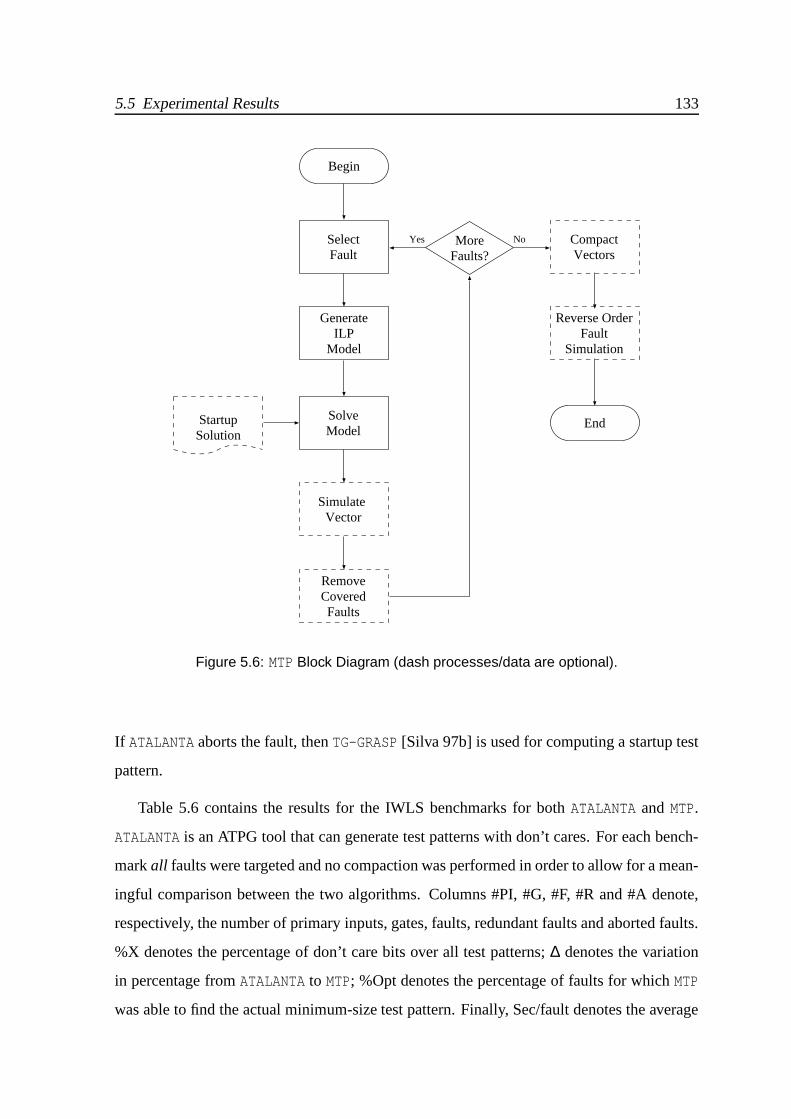
5.5 Experimental Results 133
SolveModel
End
Simulate Vector
GenerateILP
Model
RemoveCoveredFaults
CompactVectors
Reverse OrderFault
Simulation
Begin
MoreFaults?
StartupSolution
SelectFault
Yes No
Figure 5.6: MTP Block Diagram (dash processes/data are optional).
If ATALANTA aborts the fault, then TG-GRASP [Silva 97b] is used for computing a startup test
pattern.
Table 5.6 contains the results for the IWLS benchmarks for both ATALANTA and MTP.
ATALANTA is an ATPG tool that can generate test patterns with don’t cares. For each bench-
mark all faults were targeted and no compaction was performed in order to allow for a mean-
ingful comparison between the two algorithms. Columns #PI, #G, #F, #R and #A denote,
respectively, the number of primary inputs, gates, faults, redundant faults and aborted faults.
%X denotes the percentage of don’t care bits over all test patterns; ∆ denotes the variation
in percentage from ATALANTA to MTP; %Opt denotes the percentage of faults for which MTP
was able to find the actual minimum-size test pattern. Finally, Sec/fault denotes the average
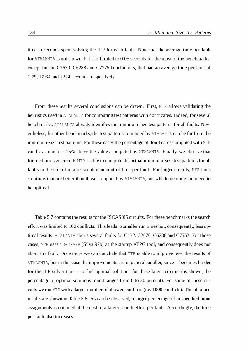
134 5. Minimum Size Test Patterns
time in seconds spent solving the ILP for each fault. Note that the average time per fault
for ATALANTA is not shown, but it is limited to 0 05 seconds for the most of the benchmarks,
except for the C2670, C6288 and C7775 benchmarks, that had an average time per fault of
1 79, 17 64 and 12 30 seconds, respectively.
From these results several conclusions can be drawn. First, MTP allows validating the
heuristics used in ATALANTA for computing test patterns with don’t cares. Indeed, for several
benchmarks, ATALANTA already identifies the minimum-size test patterns for all faults. Nev-
ertheless, for other benchmarks, the test patterns computed by ATALANTA can be far from the
minimum-size test patterns. For these cases the percentage of don’t cares computed with MTP
can be as much as 15% above the values computed by ATALANTA. Finally, we observe that
for medium-size circuits MTP is able to compute the actual minimum-size test patterns for all
faults in the circuit in a reasonable amount of time per fault. For larger circuits, MTP finds
solutions that are better than those computed by ATALANTA, but which are not guaranteed to
be optimal.
Table 5.7 contains the results for the ISCAS’85 circuits. For these benchmarks the search
effort was limited to 100 conflicts. This leads to smaller run times but, consequently, less op-
timal results. ATALANTA aborts several faults for C432, C2670, C6288 and C7552. For those
cases, MTP uses TG-GRASP [Silva 97b] as the startup ATPG tool, and consequently does not
abort any fault. Once more we can conclude that MTP is able to improve over the results of
ATALANTA, but in this case the improvements are in general smaller, since it becomes harder
for the ILP solver bsolo to find optimal solutions for these larger circuits (as shown, the
percentage of optimal solutions found ranges from 0 to 20 percent). For some of these cir-
cuits we ran MTP with a larger number of allowed conflicts (i.e. 1000 conflicts). The obtained
results are shown in Table 5.8. As can be observed, a larger percentage of unspecified input
assignments is obtained at the cost of a larger search effort per fault. Accordingly, the time
per fault also increases.
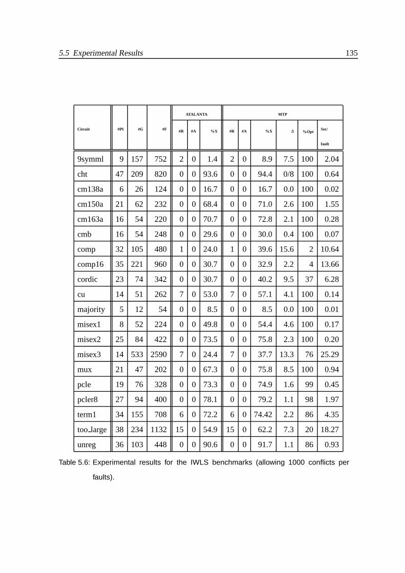
5.5 Experimental Results 135
ATALANTA MTP
Circuit #PI #G #F #R #A %X #R #A %X ∆ %OptSec/
fault
9symml 9 157 752 2 0 1.4 2 0 8.9 7.5 100 2.04
cht 47 209 820 0 0 93.6 0 0 94.4 0/8 100 0.64
cm138a 6 26 124 0 0 16.7 0 0 16.7 0.0 100 0.02
cm150a 21 62 232 0 0 68.4 0 0 71.0 2.6 100 1.55
cm163a 16 54 220 0 0 70.7 0 0 72.8 2.1 100 0.28
cmb 16 54 248 0 0 29.6 0 0 30.0 0.4 100 0.07
comp 32 105 480 1 0 24.0 1 0 39.6 15.6 2 10.64
comp16 35 221 960 0 0 30.7 0 0 32.9 2.2 4 13.66
cordic 23 74 342 0 0 30.7 0 0 40.2 9.5 37 6.28
cu 14 51 262 7 0 53.0 7 0 57.1 4.1 100 0.14
majority 5 12 54 0 0 8.5 0 0 8.5 0.0 100 0.01
misex1 8 52 224 0 0 49.8 0 0 54.4 4.6 100 0.17
misex2 25 84 422 0 0 73.5 0 0 75.8 2.3 100 0.20
misex3 14 533 2590 7 0 24.4 7 0 37.7 13.3 76 25.29
mux 21 47 202 0 0 67.3 0 0 75.8 8.5 100 0.94
pcle 19 76 328 0 0 73.3 0 0 74.9 1.6 99 0.45
pcler8 27 94 400 0 0 78.1 0 0 79.2 1.1 98 1.97
term1 34 155 708 6 0 72.2 6 0 74.42 2.2 86 4.35
too large 38 234 1132 15 0 54.9 15 0 62.2 7.3 20 18.27
unreg 36 103 448 0 0 90.6 0 0 91.7 1.1 86 0.93
Table 5.6: Experimental results for the IWLS benchmarks (allowing 1000 conflicts per
faults).

136 5. Minimum Size Test Patterns
ATALANTA MTP
Circuit #PI #G #F #R #A %X #R #A %X ∆ %OptSec/
fault
C432 36 160 524 3 1 56.2 4 0 60.8 4.6 0 3.21
C499 41 202 758 8 0 17.1 8 0 18.7 1.6 0 4.35
C880 60 383 942 0 0 82.2 0 0 83.8 1.6 12 2.54
C1355 41 546 1574 8 0 13.3 8 0 13.7 0.4 0 9.12
C1908 33 880 1878 8 0 44.7 8 0 48.4 3.7 0 9.61
C2670 233 1193 2746 97 20 92.0 117 0 92.4 0.4 23 10.99
C3540 50 1669 3425 134 0 74.6 134 0 77.3 2.7 15 16.81
C5315 178 2307 5350 59 0 92.6 59 0 92.9 0.3 14 9.34
C6288 32 2416 7744 34 387 22.2 34 0 25.1 2.9 1 36.65
C7552 207 3512 7550 77 181 86.9 131 0 86.9 0.0 4 17.46
Table 5.7: Experimental results for the ISCAS’85 benchmarks (allowing 100 conflicts per
fault).
ATALANTA MTP
Circuit #PI #G #F #R #A %X #R #A %X ∆ %OptSec/
fault
C432 36 160 524 3 1 56.2 4 0 64.1 7.9 2 27.04
C499 41 202 758 8 0 17.1 8 0 19.5 2.4 0 33.71
C880 60 383 942 0 0 82.2 0 0 85.6 3.4 40 22.34
C1355 41 546 1574 8 0 13.3 8 0 15.2 1.9 0 64.86
C1908 33 880 1878 8 0 44.7 8 0 60.0 15.3 1 73.44
C2670 233 1193 2746 97 20 92.0 117 0 93.0 1.0 25 83.46
Table 5.8: Experimental results for some of the ISCAS’85 benchmarks (allowing 1000 con-
flicts per fault).

5.6 Conclusions 137
5.6 Conclusions
Automatic test pattern generation for combinational circuits is a mature field in electronic
design automation industry. Very efficient models and algorithms exist for generation of
test patterns for stuck-at faults, regarding to fault coverage, test set size and running time.
Although, due to the heuristic nature of those algorithms, test patterns have, in general, more
specified bits than actually needed to detect a fault.
In this chapter we presented a SAT-based integer linear programming model for com-
puting minimum-size test patterns. The applicability of the model has been illustrated by
computing minimum size test patterns for the IWLS and ISCAS’85 benchmarks circuits.
From these experimental results we can draw the following conclusions: For some circuits, the heuristics used by ATALANTA (as well as by other structural
ATPG algorithms) are extremely effective and MTP can be used to formally prove this
result. Whenever the main goal is maximizing the number of don’t care bits, then MTP can be
run on top of ATALANTA (or any other ATPG algorithm), thus in general allowing for
an increased number of unspecified bit assignments. The improvements obtained by
MTP are related to the amount of allowed search effort, and MTP is always guaranteed
to produce results that are no worse than the startup tool (in our case ATALANTA or
TG-GRASP).
In the following chapters we will present some practical applications that are based on
this model and/or which benefit from the existence of a large number of unspecified inputs in
the test set. Chapter 6 proposes a model for compression of the test set, towards a reduction
of the testing time and the size of built-in self-test generators. And, Chapter 7 presents a low-
power testing technique, based on a reordering of the test vectors, which takes advantage of
the unspecified inputs in the test set.

138

Chapter 6
Maximum Test Width Compression
Contents
6.1 Introduction
6.2 BIST Circuit Generator
6.3 Test Generation With Unspecified Variable Assignments
6.4 Computing Test Patterns for Width Compression
6.4.1 Forcing Compatibility Classes
6.4.2 The Complete Optimization Model
6.5 Model/Solver Limitations
6.6 Experimental Results
6.7 Conclusions
139

140 6. Maximum Test Width Compression

6.1 Introduction 141
6.1 Introduction
In this chapter we propose a test pattern generation model targeting the reduction of the
overhead introduced by Built-In Self-Test techniques. This model is based on the test pattern
generation model with don’t cares and on the SAT solver algorithm presented in the previous
chapters.
Built-In Self-Test (BIST) denotes the ability of a circuit (or system) to test itself. This
paradigm for testing integrated circuits is widely used in the VLSI industry because it can po-
tentially eliminate the need for external test equipment and introduces the capability for test-
ing devices after the circuit is integrated in a system, in the field (on-line testing) [Abramovici 90].
The increasing use of electronics in safety critical applications also demands the use of on-
line testing. Such systems in general require testing to have a high fault coverage and be as
fast as possible. Test vectors are generated on the chip by a Test Pattern Generator (TPG)
circuit and the circuit responses are examined by an Output Response Analyzer (ORA) that
determines the correct operation of the integrated circuit [Abramovici 90, Chen 95].
One of the key challenges in BIST is the design of the TPG. An optimal TPG will gener-
ate the minimum number of test vectors (to reduce testing time) that guarantees the highest
fault coverage while introducing the minimum area overhead and performance penalty in the
circuit (in terms of circuit delay, power dissipated, etc). All these design goals are difficult to
meet simultaneously, and several architectures for TPG have been proposed [Abramovici 90].
Two alternative architectures with respect to area overhead and testing time are the ROM-
based architectures and the counter-based architectures [Abramovici 90]. The ROM-based
architectures use a ROM to store the vectors generated by an Automatic Test Pattern Genera-
tor (ATPG). Thus, high fault coverages and short testing times can be achieved. Conversely,
the area overhead introduced by this method (ROM, counter, address decoder, etc.) is in
general prohibitive for practical applications. In counter-based architectures the test patterns
are generated by counter or counter-like circuits, which introduce a small area penalty. The
main disadvantage of this method is that long test sequences may be required to achieve
acceptable fault coverages, which result in longer testing times, a drawback for time-critical
applications.

142 6. Maximum Test Width Compression
In this chapter we describe a model for ATPG targeting counter-based TPG architec-
tures. Constraints are imposed during test pattern generation which target the reduction of
the number of bits (width) of the counter used in the test generation circuit. The method
guarantees a high fault coverage (100% of non-redundant faults) with a shorter test time.
The proposed solution is based on an integer linear programming (ILP) formulation which
builds on the Propositional Satisfiability (SAT) model for test pattern generation described
in previous chapters.
This chapter is organized as follows. In the next section we start by identifying the
model and the width compression technique upon which the proposed solution is based. In
Section 6.3 we summarize the model for the generation of test patterns with unspecified
inputs presented in Chapter 5. Afterwards, in Section 6.4 we introduce the ILP test gen-
eration model that targets width compression. This model is based on the identification of
compatibility relations between primary inputs of the circuit under test. Since don’t cares
in test patterns are of key relevance for increasing the compatibility relations, we will use
the framework presented in Chapter 5 for computing test patterns with unspecified input as-
signments. In Section 6.5 we discuss some limitations of the proposed model which result
from the framework used (i.e. the supporting base model and the model solver). Finally,
on Section 6.6 we describe an ATPG tool referred as Minimum Test Pattern generator with
Width Compression (MTP-C) and include experimental results on the practical application of
the model.
6.2 BIST Circuit Generator
A large number of techniques exist for designing TPGs circuits for BIST
[Abramovici 90, Chakrabarty 98, Al-Asaad 98, Devadas 98]. A general model for a BIST
scheme is shown in Figure 6.1. The test generator circuit produces a sequence of patterns w
bits wide that can be regarded as compressed or encoded test patterns. The decoder circuit
expands or decodes these patterns into n bits wide tests, where n is the number of inputs in
the Circuit Under Test (CUT). In general, w n and the test generator circuit can be some
type of counter-like that generates all 2w patterns.

6.2 BIST Circuit Generator 143
¾¾¾¾
¿¿¿¿
ÀÁÀÁÀÂÁÂ
ÃÁÃÁÃÄÁÄ
Test Pattern Generator
(TPG)
DecoderCircuit
Test GeneratorCircuit
CombinationalCUT
w
n
Figure 6.1: Generic test pattern generator model [Chakrabarty 97].
The most common TPGs circuits used in BIST are counter-based, in which the number of
flip-flops is, in general, equal to the number of inputs of the CUT, thus the decoder circuit is
inexistent (w n). The most hardware-efficient test generator circuits, when compared with
the area of dedicated FSMs or counters, are the Linear Feed Back Registers (LFSR). These
circuits are made of flip-flops and XOR gates interconnected in certain simple configura-
tions, that present a fairly regular structure and which are able to generate exhaustive and/or
pseudo-random test sequences. Identification and design of good LFSRs, in order to produce
exhaustive and/or pseudo-random test sequences, involve detailed mathematical background
beyond the scope and purpose of this chapter1. However, tables describing common ex-
haustive LFSR can be easily found [Abramovici 90]. The example presented in Figure 6.2
illustrates that a LFSR must be carefully designed so it can be used as a TPG for BIST. The
two LFSRs presented are very similar, but only the first one (Figure 6.2(a)) can generate all
combinations of 4 bits, with the exception of 0000, for an initial non-zero vector. The second
LFSR (Figure 6.2(b)) just generates a subset of all possible combinations according to the
initial vector.
1See for example [Golomb 82, Yarmolik 88] for additional details.
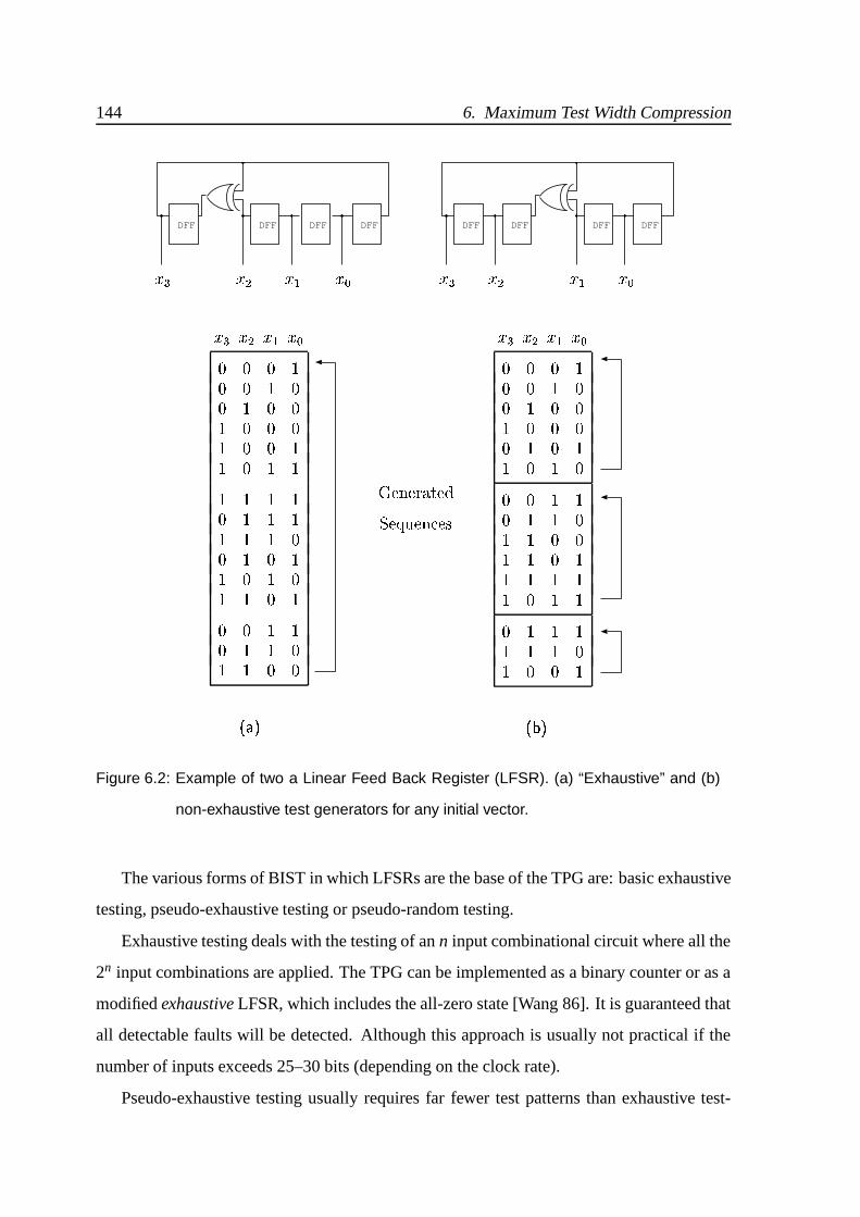
144 6. Maximum Test Width Compression
Å'ÆÇÅÉÈÊÅËÌÅÉÍÎ Î Î ÏÎ Î Ï ÎÎ Ï Î ÎÏ Î Î ÎÏ Î Î ÏÏ Î Ï ÏÏ Ï Ï ÏÎ Ï Ï ÏÏ Ï Ï ÎÎ Ï Î ÏÏ Î Ï ÎÏ Ï Î ÏÎ Î Ï ÏÎ Ï Ï ÎÏ Ï Î Î
Ð'ÑÇÐÉÒÊÐÓÌÐÉÔÕ Õ Õ ÖÕ Õ Ö ÕÕ Ö Õ ÕÖ Õ Õ ÕÕ Ö Õ ÖÖ Õ Ö ÕÕ Õ Ö ÖÕ Ö Ö ÕÖ Ö Õ ÕÖ Ö Õ ÖÖ Ö Ö ÖÖ Õ Ö ÖÕ Ö Ö ÖÖ Ö Ö ÕÖ Õ Õ Ö
×*ØHÙ ÚIÛ,Ü
DFF DFF DFF DFF
ÝÉÞßàáÉâãÉä åÉæ çÉè éÉêDFF DFF DFFDFF
ëì
íïîñðòîñóô,õQîñö÷øîñù6úòîñðòûñîñü
Figure 6.2: Example of two a Linear Feed Back Register (LFSR). (a) “Exhaustive” and (b)
non-exhaustive test generators for any initial vector.
The various forms of BIST in which LFSRs are the base of the TPG are: basic exhaustive
testing, pseudo-exhaustive testing or pseudo-random testing.
Exhaustive testing deals with the testing of an n input combinational circuit where all the
2n input combinations are applied. The TPG can be implemented as a binary counter or as a
modified exhaustive LFSR, which includes the all-zero state [Wang 86]. It is guaranteed that
all detectable faults will be detected. Although this approach is usually not practical if the
number of inputs exceeds 25–30 bits (depending on the clock rate).
Pseudo-exhaustive testing usually requires far fewer test patterns than exhaustive test-

6.2 BIST Circuit Generator 145
ing to achieve the same fault coverage. This technique relies on the partition of the CUT
in smaller logic blocks with p inputs p n , which greatly reduce the total number of
patterns to generate. Then, each block is exhaustively tested and, if possible, this is done
concurrently [Abramovici 90].
Pseudo-random testing uses a “randomly” generated subset of the 2n test patterns. Thus,
not all inputs combinations are used and the fault coverage must be determined by fault
simulation once the test generator circuit is defined. In general, long test sequences are
necessary to achieve high fault coverage, in particular for circuits that contain random-
pattern resistant faults (i.e. circuits with many hard to detect faults). Several techniques
have been proposed in order to reduce the test length at the cost of increasing the com-
plexity of the test generator circuit and/or the decoder circuit. In weighted random test-
ing [Hartmann 93, Muradali 90, Pomeranz 93a, Wunderlich 98] an extra circuit biases the
pseudo-random sequence, imposing some inputs of the CUT to predefined values based in
pre-computed weighted sets. Other techniques try to encode or include a deterministic test
set in the test generator circuit either searching the appropriate seeds [Lempel 95] or by using
multiple seeds and select the LFSR that best covers the test set through the use of reconfig-
urable LFSRs [Dufaza 91, Hellebrand 95a, Hellebrand 95b] or by using some mapping logic
between the test generator circuit and the CUT [Chatterjee 95, Touba 95a, Touba 95b].
Previous work in BIST [Chakrabarty 97, Chen 95] has led to a new procedure for the
generation of test generator circuits which target the minimization of the number of required
flip-flops. This procedure is based on the compression of the width (i.e. the number of bits)
of the original test patterns. Therefore, a smaller counter-based FSM is used to generate the
compressed test patterns (with a width of w bits, such that w n) which are then fed to the
decoder circuit. The test pattern generated by the decoding logic is then applied to the circuit
under test. The main advantage of this technique is that at the same time we are reducing the
area of the test generator circuit, we are also cutting down the test time, without introducing
additional logic in the decoder circuit. Note that the counting time is cut by half for each bit
reduced and consequently, the power dissipated during the test is also reduced.
Width compression was proposed by Chen and Gupta [Chen 95] who observed that in
many cases, some inputs of the CUT can be physically connected to the same output of the
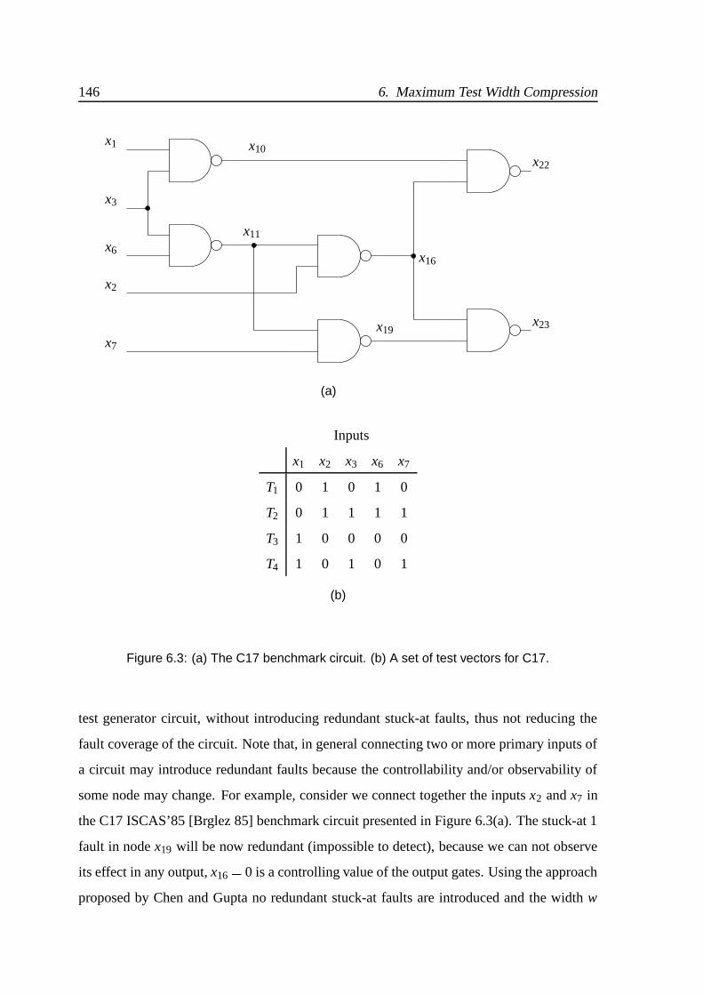
146 6. Maximum Test Width Compression
x1
x3
x6
x10
x11
x19
x16
x22
x23
x7
x2
(a)
Inputs
x1 x2 x3 x6 x7
T1 0 1 0 1 0
T2 0 1 1 1 1
T3 1 0 0 0 0
T4 1 0 1 0 1
(b)
Figure 6.3: (a) The C17 benchmark circuit. (b) A set of test vectors for C17.
test generator circuit, without introducing redundant stuck-at faults, thus not reducing the
fault coverage of the circuit. Note that, in general connecting two or more primary inputs of
a circuit may introduce redundant faults because the controllability and/or observability of
some node may change. For example, consider we connect together the inputs x2 and x7 in
the C17 ISCAS’85 [Brglez 85] benchmark circuit presented in Figure 6.3(a). The stuck-at 1
fault in node x19 will be now redundant (impossible to detect), because we can not observe
its effect in any output, x16 0 is a controlling value of the output gates. Using the approach
proposed by Chen and Gupta no redundant stuck-at faults are introduced and the width w
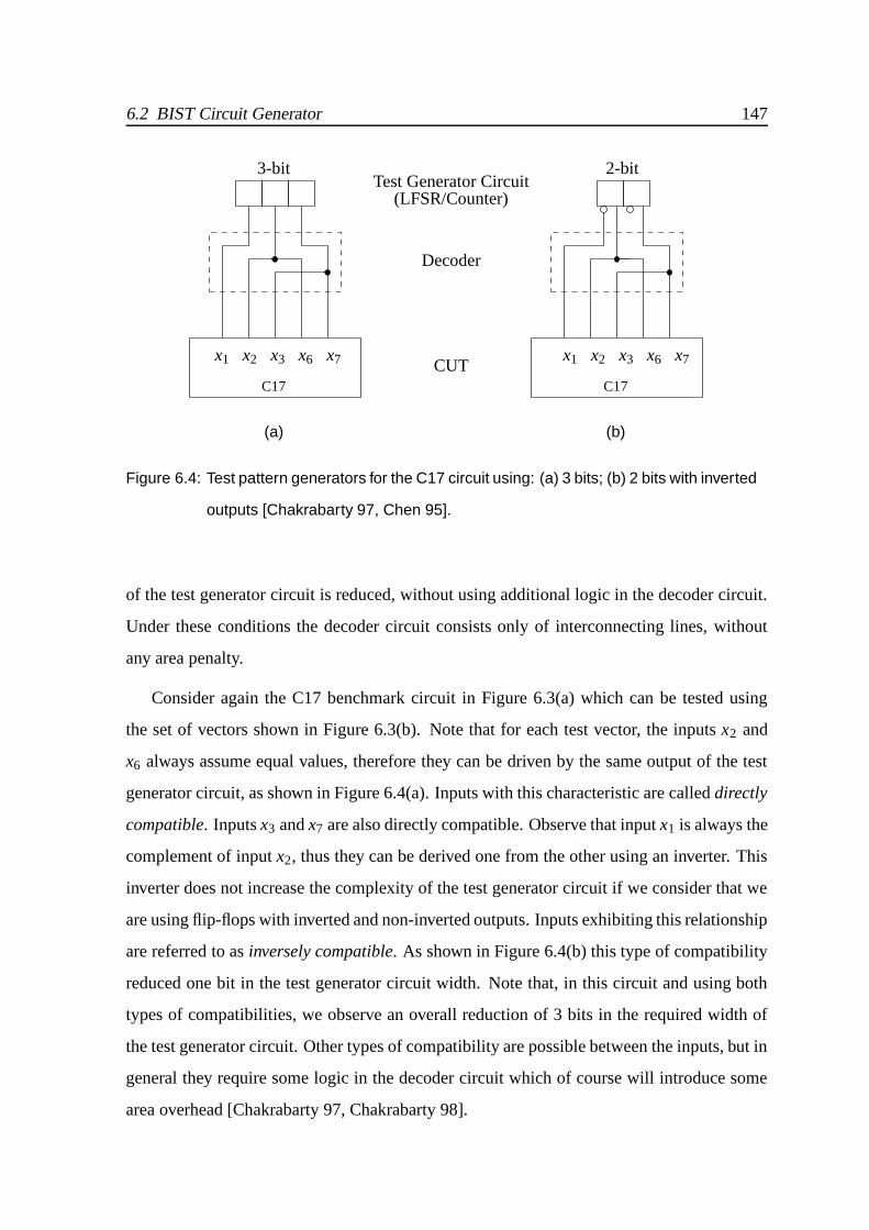
6.2 BIST Circuit Generator 147
(a) (b)
Test Generator Circuit(LFSR/Counter)
x6 x7x1 x2 x3
3-bit
C17
x6 x7x1 x2 x3
2-bit
C17
Decoder
CUT
Figure 6.4: Test pattern generators for the C17 circuit using: (a) 3 bits; (b) 2 bits with inverted
outputs [Chakrabarty 97, Chen 95].
of the test generator circuit is reduced, without using additional logic in the decoder circuit.
Under these conditions the decoder circuit consists only of interconnecting lines, without
any area penalty.
Consider again the C17 benchmark circuit in Figure 6.3(a) which can be tested using
the set of vectors shown in Figure 6.3(b). Note that for each test vector, the inputs x2 and
x6 always assume equal values, therefore they can be driven by the same output of the test
generator circuit, as shown in Figure 6.4(a). Inputs with this characteristic are called directly
compatible. Inputs x3 and x7 are also directly compatible. Observe that input x1 is always the
complement of input x2, thus they can be derived one from the other using an inverter. This
inverter does not increase the complexity of the test generator circuit if we consider that we
are using flip-flops with inverted and non-inverted outputs. Inputs exhibiting this relationship
are referred to as inversely compatible. As shown in Figure 6.4(b) this type of compatibility
reduced one bit in the test generator circuit width. Note that, in this circuit and using both
types of compatibilities, we observe an overall reduction of 3 bits in the required width of
the test generator circuit. Other types of compatibility are possible between the inputs, but in
general they require some logic in the decoder circuit which of course will introduce some
area overhead [Chakrabarty 97, Chakrabarty 98].

148 6. Maximum Test Width Compression
The utilization of pre-computed test patterns with don’t cares can significantly simplify
the test generator circuit by reducing its width w. Test sets with don’t cares are in general
larger than full specified test sets, but the number of compatibility inputs may be greater,
because don’t care bits can be chosen to force some type of compatibility, reducing the
test generator circuit width. Nevertheless, using a general ATPG which produces test sets
with don’t cares may not be sufficient for a good width compression, because each vector
is determined to detect a fault without any consideration regarding input compatibilities of
already computed test patterns.
It is important that the notion of compatibility be present during the ATPG process, so
that each vector detects one or more target faults but, at the same time, keeps the compati-
bility between inputs as much as possible. In our model we only consider direct and inverse
compatibilities in the situations where test patterns exhibit don’t cares. The objective will be
to minimize the width w of the test generator circuit such that all non-redundant circuit faults
are detected.
6.3 Test Generation With Unspecified Variable Assignments
In order to maximize the number of compatibility relations, test patterns are required to
exhibit don’t cares, thus we base our approach on the test generation model presented in
Section 5.2. In summary, we recall that: Each circuit node variable x was split in two new variables x1 and x0, according to
the mapping presented in Table 5.1 (page 120). The invalid combination 1 1 was
excluded by the inclusion of the additional constraint ϕinv x (5.2) for each node. The CNF formulas that represent the valid assignments of each gate were re-written
so that the inputs and the output exhibit the correct behavior in the presence of don’t
cares. The resulting generalized CNF formulas for the simple gates that use the new
variables were presented in Table 5.3 (page 124). The CNF formulas for computing the faulty values of a node are similar to the ones
that compute the good values for the same node. Although, as shown in (5.9), an

6.4 Computing Test Patterns for Width Compression 149
unspecified value in the good variables implies an unspecified assignment in the faulty
variables. Hence, the resulting CNF formula (5.11), for a faulty node xF , avoids
propagating a specified value in the faulty circuit while in the real circuit the node
value is not defined as 0 or 1. The definition of the sensitization status variable xS of each node was also changed
to consider unspecified inputs. Table 5.4 (page 128) shows the new definition of
the sensitization status variables. It reflects the usual XOR behavior between good
and faulty variables, when both are specified, and assumes value 0 when the faulty
variables is specified with a don’t care value. This guarantees the correct propagation
of the fault effect independently of the values that unspecified variables assume during
real circuit testing.
In the remainder of this chapter we use the framework proposed for computing test pat-
terns with don’t cares that is summarized in Table 5.5 (see page 129).
6.4 Computing Test Patterns for Width Compression
In this section we develop a greedy optimization model for computing test patterns aim-
ing at the reduction of the width of the test set. As already mentioned, this optimization
model is based on test pattern generation in the presence of incompletely specified primary
input assignments.
6.4.1 Forcing Compatibility Classes
A compatibility class is defined as a set of inputs which can be connected together, or
through an inverter. Thus, such inputs can be driven only by one output of the test generator
circuit throughout the application of the complete test sequence. Formally we can define
directly and inversely compatibility inputs as follows:

150 6. Maximum Test Width Compression
Definition 6.1 (Compatible inputs) Consider a set of test vectors V T1 T2 TN . Two inputs xi and x j are directly compatible in the set V if
ýTp V Tp þ i ÿ( Tp þ j ÿ or Tp þ i ÿ9 X or Tp þ j ÿ9 X
and are inversely compatible in set V if
ýTp V Tp þ i ÿ( Tp þ j ÿ or Tp þ i ÿ9 X or Tp þ j ÿ9 X
Two inputs are totally compatible in a set V if they are simultaneously directly and in-
versely compatible, and just compatible if they are compatible in any of the previous ways.
We can now define sets of compatibility classes and the set of compatibility pairs using
the compatibility relations defined above. The former will identify the sets of inputs that will
be driven by one output (and its negation) of the test generator circuit. The latter, will list all
the pairs of inputs that are compatible. Formally, these sets are defined as follows:
Definition 6.2 (Compatibility class) A compatibility class, Θi, is a maximal set of inputs
that are compatible amongst themselves, for a given group of test vectors.
Definition 6.3 (Set of compatibility pairs) The set of compatibility pairs, Ω, is the set of all
pairs of inputs that, for a given group of test vectors, are compatible (directly or inversely).
For example, in the C17 benchmark circuit and considering the set of test vectors, V T1 T2 T3 T4 , presented in Figure 6.3(b). As shown before, in this set of test vectors, x2 x6 and x3 x7
are directly compatible pairs of inputs, and x1 x2 and x1 x6
are in-
versely compatible pairs of inputs. So, the set compatibility pairs for the test vectors in V
is Ω x2 x6 x3 x7
x1 x2 x1 x6
. The two existing compatibility classes for these
vectors are Θ1 x1 x2 x6 and Θ2 x3 x7 .Finding the optimum set of compatibility classes for a set of test vectors can be reduced to
the clique problem2, by representing our problem on a graph whose vertices are the primary
inputs and the edges correspond to the compatibility relation between the inputs. Deter-
mining the maximal clique size on this graph, which is an NP-complete problem [Aho 74,
2See footnote on page 47 for a clique definition.

6.4 Computing Test Patterns for Width Compression 151
Cormen 90], corresponds to identifying the optimum set of compatibility classes. The usual
approaches for solving these problems are based on heuristic or approximation algorithms.
Therefore, we use a heuristic approach to efficiently generate good classes in practice.
A heuristic algorithm that produces a good set of compatibility classes is presented
in [Chakrabarty 97]. We will use this algorithm as our general procedure for identifying,
at the end when the whole set of vectors is determined, the resulting compatibility classes.
Basically, this algorithm identifies directly and inversely compatible inputs, for a given test
set, and represents them on a graph as described above. Then, heuristically, the proce-
dure identifies an initial set of cliques with size 3, which can be identified in polynomial
time [Garey 79, Chakrabarty 97]. Finally, vertices are iteratively added to the cliques if the
compatibility is maintained between all the nodes in the clique.
When determining a test vector for a given target fault we would like to keep the same
cardinality on the set of compatibility pairs (cp Ω ) already found from previous test
vectors. Note that, for each new vector that is added to the set of test vectors V , the new
value of cp may only be equal to or less than the previous value. It will be equal, if the
existing compatibilities between pairs of inputs are not broken by the new vector and less
otherwise. Hence, from all the vectors that detect a new target fault, we would like to select
the one that does not decrease cp, thus keeping the number of compatible inputs as large as
possible. We will define some extra boolean variables that constrain the search process with
the objective of finding such vectors.
The compatibility variables, Ci j, are associated with each element in the set of compat-
ibility pairs, Ω. The role of this variable in the model is to identify which pair of inputs xi x j Ω are still compatible after a new vector is computed. As shown in Table 6.1 this
variable assumes value 1 when the compatibility between inputs xi and x j does not hold due
to the new vector, and 0 otherwise. Considering that each circuit node x is represented in the
model by two variables, x0 and x1, according to Table 5.1, the CNF clauses ϕCi j which define
the compatibility variables for direct and inverse compatible inputs are the following3:
3Each CNF formula is a product-of-sums of the consistency function (ξ) of the function that define the Ci jvariable, as presented in Table 6.1.

152 6. Maximum Test Width Compression
Inputs Ci j Ui j Si jxi x j Direct Total Inverse
X X 0 0 0 0 0
X 0 0 0 0 1 0
X 1 0 0 0 1 0
0 X 0 0 0 1 0
0 0 0 0 1 1 1
0 1 1 0 0 1 1
1 X 0 0 0 1 0
1 0 1 0 0 1 1
1 1 0 0 1 1 1
Table 6.1: Definition of variables Ci j, Ui j and Si j.
ϕCi j !
4: x1i _: x0
j Ci j ¥ x1i x1
j _: Ci j if xi and x j are4: x0i _: x1
j Ci j ¥ x0i x0
j _: Ci j directly compatible
4: Ci j if xi and x j are totally compatible
4: x1i _: x1
j Ci j ¥ x1i x0
j _: Ci j if xi and x j are4: x0i _: x0
j Ci j ¥ x0i x1
j _: Ci j inversely compatible
(6.1)
Moreover, in order to enhance future compatibility classes we add to our model two
more types of boolean variables. The use of these new variables will allow us to select vec-
tors that, besides detecting a target fault and hold the compatibility between pairs of inputs xi x j Ω, they also have a lower number of specified values on those input pairs. Note
that, according to Definition 6.1, inputs with unspecified values can be simultaneous directly
and inversely compatible. So, by selecting vectors with unspecified inputs in the compat-
ibility pairs, we are postponing the exclusion of some compatibility types. For example,

6.4 Computing Test Patterns for Width Compression 153
let us consider two test sequences in the inputs pair xi x j : S1 X 0 1 0 0 0 and
S2 X 0 X 1 0 0 . For the S1 set of assignments direct compatibility is excluded
by the second vector and the inverse compatibility by the third vector, which turns these two
inputs as not compatible. For the set of assignments S2, only the third vector excludes inverse
compatibility, which keeps these two inputs as compatible. Therefore, the definition of the
new variables types should let us distinguish for each pair of inputs xi x j Ω, of a new
vector, the following three situations:
1. both inputs are unspecified;
2. one of the inputs is specified and the other is unspecified;
3. both inputs are specified.
The unity variables, Ui j, allow us to identify when any pair of inputs in a set of compat-
ibility pairs of a new test vector is specified. Using this variable we will give preference to
vectors with both inputs unspecified (case Ui j 0). Table 6.1 presents the values assigned
to this variable for any valid combination of the bit values in a pair of previously compatible
inputs. The CNF formula ϕUi j that captures the Ui j behavior is:
ϕUi j 4: x0i Ui j 4: x1
i Ui j ¥4: x0j Ui j ¥P: x1
j Ui j x1i x0
i x1j x0
j : Ui j (6.2)
The simultaneity variables, Si j, let us determine when both of the inputs are specified.
Table 6.1 also describes the values assigned to simultaneity variables, Si j, for any valid
combination of two inputs in the set of compatibility pairs. By selecting test vectors with
this variable equal to 0, we guarantee that at most one of the two inputs is unspecified. The
CNF formula ϕSi j that captures this behavior is:

154 6. Maximum Test Width Compression
ϕSi j 4: x0i _: x0
j Si j ¥P: x0i : x1
j Si j x1i x0
i _: Si j 4: x1i _: x0
j Si j ¥P: x1i : x1
j Si j x1j x0
j _: Si j (6.3)
As we will explain below, with these variables we are able to increase the number of
unspecified inputs in each test pattern within a compatibility class.
In Figure 6.5 we present an example that exemplifies the use of these new variables and,
at the same time, illustrates the advantage of selecting test patterns with unspecified values
in compatible inputs. We assume a circuit with 4 inputs, x1 x2 x3 x4 , for which we want
to detect several faults (A, B, C, ). In this circuit the fault A is detected by the unique test
pattern TA 0 0 0 0 and the fault C is detect by the unique test pattern TC 0 0 1 0 . For
the detection of fault B is sufficient to force x3 0 and x4 1, so, we have 32 9 possible
test patterns which detect the fault B. Note that we are assuming that assignments to other
inputs can be unspecified. Let us consider four distinct cases represented by the patterns
TB1 0 1 0 1 , TB2 0 0 0 1 , TB3 X 0 0 1 and TB4 X X 0 1 . Figure 6.5 shows
the values of the variables Ci j, Ui j and Si j for the compatible inputs x1 and x2. By selecting
the vector with the lower value of the arithmetic sum on variables on Ci j, Ui j and Si j we can
identify the test pattern for which the compatibility is preserved and has more unspecified
inputs.
Figure 6.5 also shows the evolution of the compatibility graph and the corresponding
compatibility classes, Θi, for the different sequences of test patterns. Note that it may seem
indifferent to select any test pattern TBi to detect fault B, because all the resulting test se-
quences present two compatibility classes (but with a different number of compatible inputs,
as seen in the number of edges in each the graph). However, the next test pattern which
detects fault C breaks the compatibility between inputs x1 x3 and x2 x3
, thus only the
sequence with the test pattern TB4 maintains two compatibility classes while all others se-
quences increase them to three, and thus requiring one more bit in the counter of the TPG.
For this reason, the selection promotes vectors with more bits unspecified in the compatible
inputs pairs.
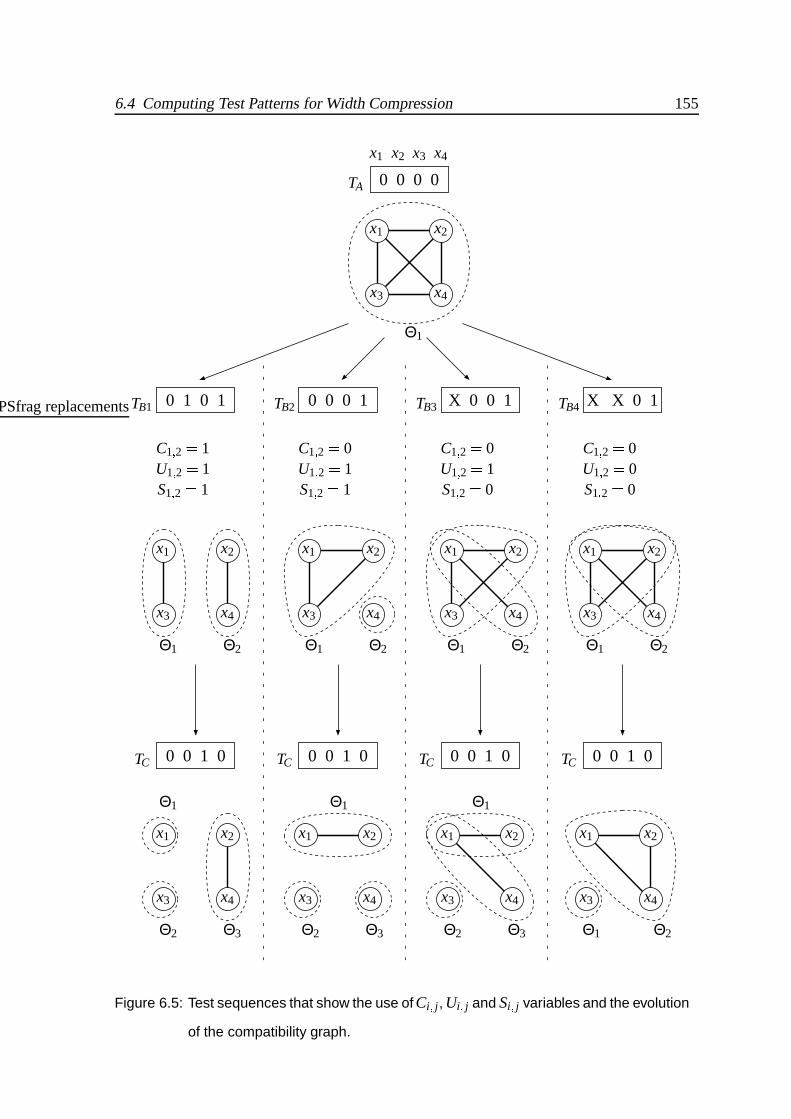
6.4 Computing Test Patterns for Width Compression 155
0 0 1 0 0 0 1 0 0 0 1 0 0 0 1 0
0 1 0 1 0 0 0 1 X 0 0 1 X X 0 1
0 0 0 0
PSfrag replacements
x1x1
x1x1x1
x1
x1x1
x1
x1
x2x2
x2x2x2
x2
x2x2
x2
x2
x3x3
x3x3x3
x3
x3x3
x3
x3
x4x4
x4x4x4
x4
x4x4
x4
x4
TA
TB1 TB2 TB3 TB4
TCTCTCTC
C1 2 1 C1 2 0C1 2 0C1 2 0U1 2 1U1 2 1U1 2 1 U1 2 0
S1 2 1S1 2 1 S1 2 0S1 2 0
Θ1Θ1
Θ1Θ1Θ1
Θ1
Θ1
Θ1
Θ1
Θ2Θ2
Θ2Θ2Θ2
Θ2Θ2
Θ2
Θ3Θ3 Θ3
Figure 6.5: Test sequences that show the use of Ci j, Ui j and Si j variables and the evolution
of the compatibility graph.
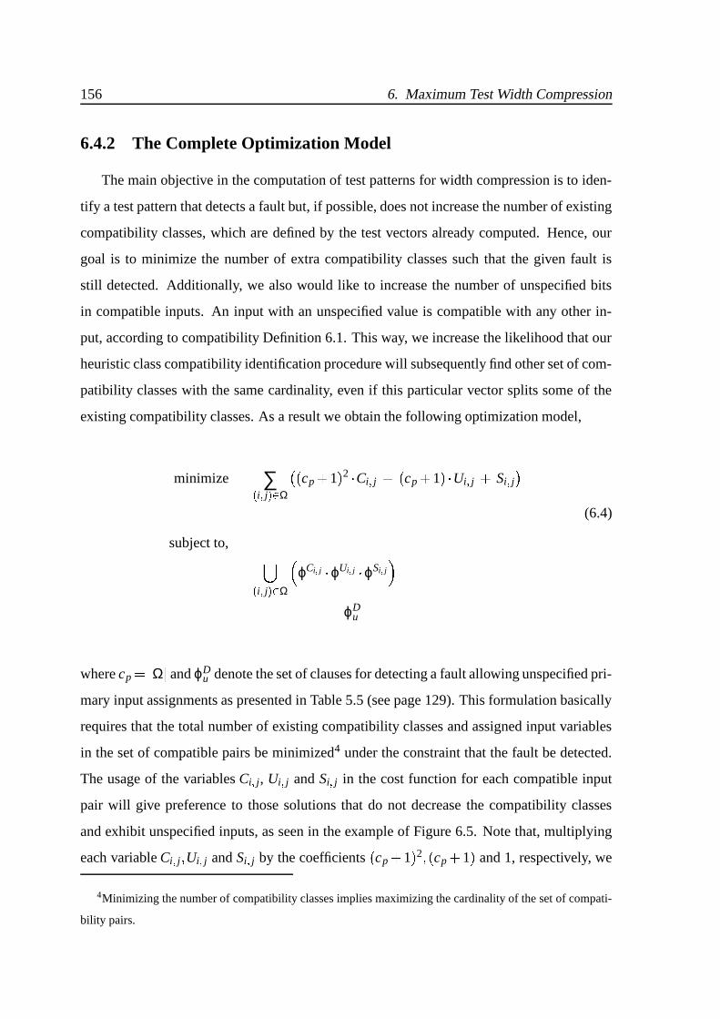
156 6. Maximum Test Width Compression
6.4.2 The Complete Optimization Model
The main objective in the computation of test patterns for width compression is to iden-
tify a test pattern that detects a fault but, if possible, does not increase the number of existing
compatibility classes, which are defined by the test vectors already computed. Hence, our
goal is to minimize the number of extra compatibility classes such that the given fault is
still detected. Additionally, we also would like to increase the number of unspecified bits
in compatible inputs. An input with an unspecified value is compatible with any other in-
put, according to compatibility Definition 6.1. This way, we increase the likelihood that our
heuristic class compatibility identification procedure will subsequently find other set of com-
patibility classes with the same cardinality, even if this particular vector splits some of the
existing compatibility classes. As a result we obtain the following optimization model,
minimize ∑0 i j 2 . Ω
§ cp 1 2 Ci j cp 1 Ui j Si j ¨(6.4)
subject to, ,0 i j 2 . Ω
ϕCi j ϕUi j ϕSi j ϕD
u
where cp Ω and ϕDu denote the set of clauses for detecting a fault allowing unspecified pri-
mary input assignments as presented in Table 5.5 (see page 129). This formulation basically
requires that the total number of existing compatibility classes and assigned input variables
in the set of compatible pairs be minimized4 under the constraint that the fault be detected.
The usage of the variables Ci j, Ui j and Si j in the cost function for each compatible input
pair will give preference to those solutions that do not decrease the compatibility classes
and exhibit unspecified inputs, as seen in the example of Figure 6.5. Note that, multiplying
each variable Ci j Ui j and Si j by the coefficients cp 1 2 cp 1 and 1, respectively, we
4Minimizing the number of compatibility classes implies maximizing the cardinality of the set of compati-
bility pairs.

6.4 Computing Test Patterns for Width Compression 157
are promoting the selection of a vector that satisfies our objectives in terms of compatibility,
besides detecting the fault (imposed by the constraints (6.4)). Having this cost function is
equivalent to say that we are selecting vectors using the following rules:
first, from the vectors that detect the given fault, we select the ones which have the
minimum number of input compatibilities breaks (Ci j 0), then, from these set we choose the vectors that have the minimum number compati-
bilities inputs pairs with any bit specified (Ui j 0), finally, from these we select the vector that in all pairs of compatible inputs has a
minimum number of specified inputs (Si j 0).
Notice that, when there are no compatibility classes, which implies an empty set of com-
patibility pairs (Ω /0), none of the variables for compatibility, unity and simultaneity are
defined. In that case, the cost function to minimize is redefined to minimize the number of
specified inputs in the test pattern, as described in the previous chapter, Section 5.3, thus the
cost function will then be:
minimize ∑xi . PI
x0i x1
i (6.5)
Observe that, once there exist no more compatibility inputs pairs (Ω /0), the number
of specified inputs in future test vectors is irrelevant with respect to input compatibility.
However, if we have a test set with more don’t cares we expect to synthesize a smaller
counter based test generator circuit (FSM).
Given the mapping between CNF clauses and linear inequalities described in Section 3.3,
the optimization problem (6.4) can be viewed as an integer linear program, and so different
integer linear optimization packages can potentially be applied. Nevertheless, the constraints
of (6.4) are tightly related with propositional satisfiability. Consequently, and as shown in

158 6. Maximum Test Width Compression
Section 3.4, SAT based ILP solvers are preferable for solving ILPs for which the constraints
correspond to CNF formulas.
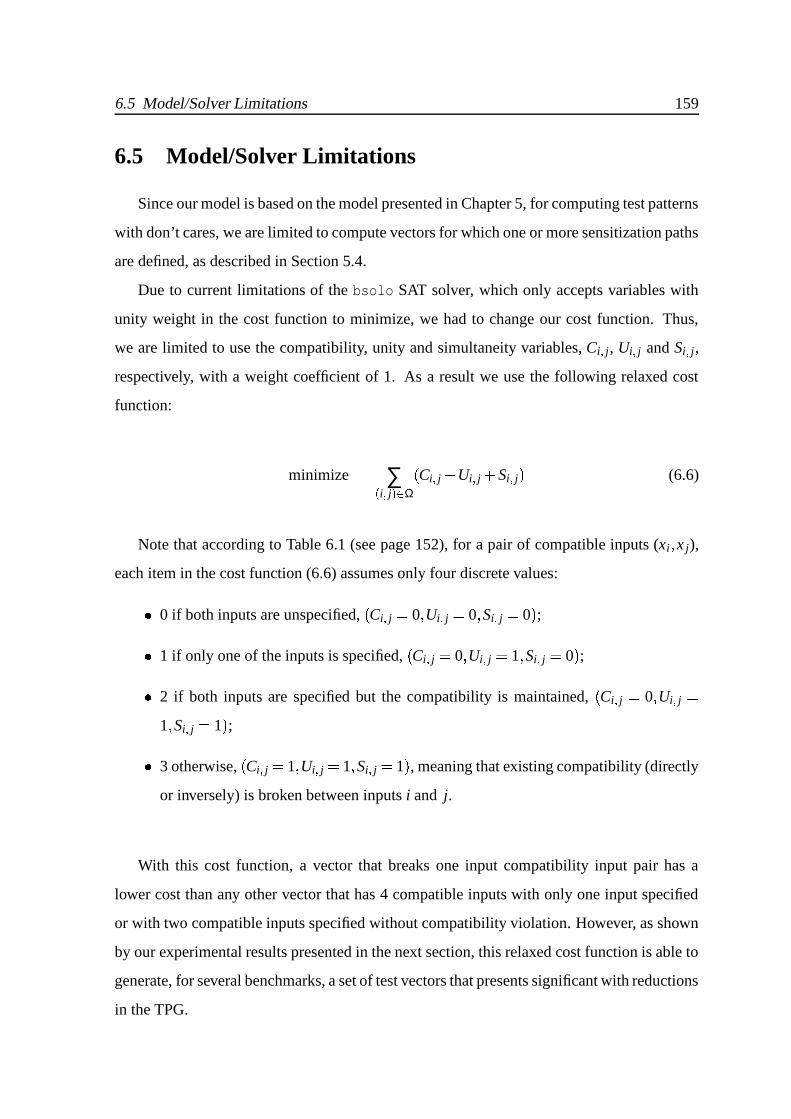
6.5 Model/Solver Limitations 159
6.5 Model/Solver Limitations
Since our model is based on the model presented in Chapter 5, for computing test patterns
with don’t cares, we are limited to compute vectors for which one or more sensitization paths
are defined, as described in Section 5.4.
Due to current limitations of the bsolo SAT solver, which only accepts variables with
unity weight in the cost function to minimize, we had to change our cost function. Thus,
we are limited to use the compatibility, unity and simultaneity variables, Ci j, Ui j and Si j,respectively, with a weight coefficient of 1. As a result we use the following relaxed cost
function:
minimize ∑0 i j 2 . Ω Ci j Ui j Si j (6.6)
Note that according to Table 6.1 (see page 152), for a pair of compatible inputs (xi x j),
each item in the cost function (6.6) assumes only four discrete values: 0 if both inputs are unspecified, Ci j 0 Ui j 0 Si j 0 ; 1 if only one of the inputs is specified, Ci j 0 Ui j 1 Si j 0 ; 2 if both inputs are specified but the compatibility is maintained, Ci j 0 Ui j 1 Si j 1 ; 3 otherwise, Ci j 1 Ui j 1 Si j 1 , meaning that existing compatibility (directly
or inversely) is broken between inputs i and j.
With this cost function, a vector that breaks one input compatibility input pair has a
lower cost than any other vector that has 4 compatible inputs with only one input specified
or with two compatible inputs specified without compatibility violation. However, as shown
by our experimental results presented in the next section, this relaxed cost function is able to
generate, for several benchmarks, a set of test vectors that presents significant with reductions
in the TPG.

160 6. Maximum Test Width Compression
6.6 Experimental Results
The model described in the previous section (with the relaxed cost function (6.6)) has
been integrated in a test pattern generation framework for the computation of test patterns
referred to as Minimum Test Pattern generator with Width Compression (MTP-C), which uses
the SAT-based ILP algorithm bsolo (described in Section 3.3.2) and the fault simulator
provided with ATALANTA [Lee 93]. The results included below were obtained with the IWLS
benchmark suite [IWLS 89] and with the ISCAS’85 benchmark suite [Brglez 85]. In all
cases MTP-C was run with a bound on the amount of allowed search (i.e. the total number of
conflicts was limited to 1000). This permits MTP-C to identify acceptable solutions, which in
some cases may not necessarily be optimal. Moreover, in order to facilitate the optimization
process, MTP-C uses the solution computed by ATALANTA (or by any other ATPG tool) as
the startup assignment. These assignments provide an initial upper bound on the value of
the optimal solution. If ATALANTA aborts the fault, then TG-GRASP [Silva 97b] is used for
computing a startup test pattern.
Table 6.2 contains the results for the IWLS benchmarks for both ATALANTA and MTP-C.
Columns #PI, #V and W denote, respectively, the number of primary inputs, the number of
test vectors and the width of test set after compression. The last two columns represent the
number of bits gained by our ATPG over ATALANTA and the average time to solve the model
for each vector (on a Sun Sparc-Ultra I with 384 Meg. of memory).
From these results we can conclude that the model implemented by the MTP-C ATPG
decreases the number of bits necessary to fully test a circuit. This is achieved by computing
fewer test vectors than ATALANTA and, in some cases, reducing the width, in the number of
bits, necessary to “store” the test patterns. We should notice that a reduction by one bit in
the width of the test patterns will reduce to half the number of test patterns produced by the
BIST generator, thus will cut down to half the time required to fully test the circuit.
Table 6.3 contains the results for the ISCAS’85 circuits. Once more we can conclude
that MTP-C is able to improve over the ATALANTA results, and in this case the improvements
are in general higher. This may happen because now we are dealing with larger circuits, so
the number of distinct vectors that can detect a given fault is in general greater, therefore it
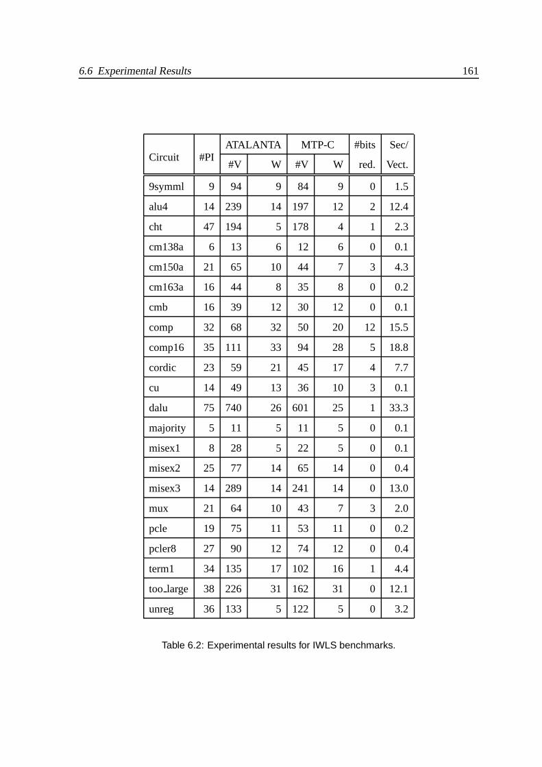
6.6 Experimental Results 161
ATALANTA MTP-C #bits Sec/Circuit #PI
#V W #V W red. Vect.
9symml 9 94 9 84 9 0 1.5
alu4 14 239 14 197 12 2 12.4
cht 47 194 5 178 4 1 2.3
cm138a 6 13 6 12 6 0 0.1
cm150a 21 65 10 44 7 3 4.3
cm163a 16 44 8 35 8 0 0.2
cmb 16 39 12 30 12 0 0.1
comp 32 68 32 50 20 12 15.5
comp16 35 111 33 94 28 5 18.8
cordic 23 59 21 45 17 4 7.7
cu 14 49 13 36 10 3 0.1
dalu 75 740 26 601 25 1 33.3
majority 5 11 5 11 5 0 0.1
misex1 8 28 5 22 5 0 0.1
misex2 25 77 14 65 14 0 0.4
misex3 14 289 14 241 14 0 13.0
mux 21 64 10 43 7 3 2.0
pcle 19 75 11 53 11 0 0.2
pcler8 27 90 12 74 12 0 0.4
term1 34 135 17 102 16 1 4.4
too large 38 226 31 162 31 0 12.1
unreg 36 133 5 122 5 0 3.2
Table 6.2: Experimental results for IWLS benchmarks.

162 6. Maximum Test Width Compression
ATALANTA MTP-C #bits Sec/Circuit #PI
#V W #V W red. Vect.
C432 36 148 31 107 24 7 25.7
C499 41 103 41 66 40 1 42.4
C880 60 393 30 289 29 1 28.2
C1355 41 145 41 96 37 3 77.9
C1908 33 291 31 181 29 2 46.3
C2670 233 780 55 600 52 3 91.0
C3540 50 718 30 530 31 -1 98.4
C5315 178 1393 38 993 44 -6 224.7
C6288 32 248 32 58 32 0 326.3
C7552 207 919 101 706 93 8 166.8
Table 6.3: Experimental results for ISCAS’85 benchmarks.
will be “easier” for the ILP solver to find vectors that meet the restrictions on compatibility
classes. The results obtained on circuits C3540 and C5315 show that our greedy approach
and/or the use of the relaxed cost function may not produce good results for all circuits.
6.7 Conclusions
In this chapter we introduce a SAT-based integer linear programming model for com-
puting test patterns for width compression. Based on the model for computing test patterns
with unspecified inputs, presented in Chapter 5, we describe an ATPG tool (MTP-C) which
incorporates several heuristics. The applicability of the model using a relaxed cost function
was illustrated by computing test patterns for the IWLS and ISCAS’85 benchmarks circuits.
From these results we can conclude that for some circuits our approach can reduce the test
patterns width, which has a significant impact on the test time and area of the test generator
circuit.
The heuristics incorporated in the MTP-C ATPG tool ought to be tuned in order to achieve
6.7 Conclusions 163
better width compression in a wider range of circuits. Introducing a fault ordering mech-
anism process and improving the compatibility selection algorithm are some of the tech-
niques that should be considered for further improvement. In addition, a solver that ac-
cepts generic linear cost functions should be used. We should also note that counter-based
test generation circuits are only practical provided we are able to reduce the width to no
more than 25–30 bits. Hence, for several of the benchmarks, additional width compres-
sion is required. We should consider determining new types of compatibility (such as d-
compatibility [Chakrabarty 97] or based on simple logic functions, i.e. OR, AND or other
2-inputs simple gates) to be incorporated in the model with the objective of reducing the
test patterns width without a significantly increase in the area of the decoder. In addition,
the techniques developed for pseudo-exhaustive testing (partition of the CUT in small logic
blocks to reduce the testing time) should also be studied for inclusion in the model.

164
Chapter 7
Power Reduction During Testing
Contents
7.1 Introduction
7.2 Power Dissipation Model
7.3 Reordering Test Patterns for Power Reduction
7.3.1 Model for Completely Specified Test Patterns
7.3.2 Reordering Test Patterns with Don’t Cares
7.4 A Formal Model for Pattern Sequence Reordering Using Don’t Cares
7.4.1 A 0-1 ILP Model for the TSP
7.4.2 An ILP Model for Pattern Reordering Using Don’t Cares
7.5 Power Reduction Algorithms
7.6 Experimental Results
7.6.1 IWLS Benchmarks
7.6.2 ISCAS Benchmarks
7.7 Conclusions
165

166 7. Power Reduction During Testing

7.1 Introduction 167
7.1 Introduction
We have seen that many circuits today include on-chip structures that enable circuit self-
testing, known as built-in self-test (BIST) [Abramovici 90]. Initially designed to make the
testing of circuits out of the fabrication line easier, they also allow for the periodic testing
of the circuit. This can be especially important for circuits used in safety-critical and/or
mobile devices. Clearly the penalty to pay is the extra circuitry required for BIST. As dis-
cussed in Chapter 6, one approach to reduce this overhead is to use a simple linear feedback
shift register (LFSR) to generate a pseudo-random input sequence, which is run until a target
fault coverage has been achieved [Abramovici 90, Chakrabarty 97]. The disadvantage of this
solution is that for high fault coverages the run time may become too long and the power dis-
sipated too high. Techniques to cope with these problems have been proposed [Manich 00],
based on filtering the non-detecting vectors (to avoid stimulating the circuit under test with
non-detecting vectors) and/or by re-seeding the LFSR (to skip a set of undesired vectors
until the next detecting vector). A different approach is to use an automated test-pattern
generator (ATPG) tool to obtain a (ideally minimum) set of test patterns necessary for the
desired fault coverage. Then, the BIST structure, that generates each of these patterns se-
quentially, reduces to a counter-type finite state machine (FSM) which could benefit from the
techniques presented in Chapter 6. Even though this solution in general requires larger area,
it is also clear that it provides shorter test sequences, thus being the option of choice for spe-
cific applications where power, and not area, is the most important design goal. Moreover,
the increased use of periodic testing in safety-critical and/or mobile devices raises concerns
about the power that is consumed during this process. Consequently, techniques for reducing
the power dissipation during testing are particularly relevant for these devices.
In this chapter we address the problem of power reduction during testing. Even though
solutions for solving this problem have so far consisted on reordering sequences of com-
pletely specified test patterns [Chakravarty 94], one might expect the potential existence of
don’t cares in test patterns to help further reducing the power dissipation during testing. The
main purpose of this chapter is to propose solutions for this problem and provide compre-
hensive empirical evidence that the existence of don’t cares in test patterns can in fact play a

168 7. Power Reduction During Testing
significant role in reducing power dissipation during testing.
This chapter is organized as follows. We start in Section 7.2 by introducing the power
dissipation model for CMOS digital circuits. In Section 7.3 we describe a model for reducing
power dissipation during testing whenever test patterns are completely specified. Moreover,
we relate this problem to the problem of minimizing the sum of the Hamming distances
between pairs of tests in a test sequence. In this same section we also consider approaches
for using test patterns containing don’t cares and analyze the problem of reducing power
during the application of these test pattern sequences. Afterwards, in Section 7.4, we derive a
formal optimization model for the problem of minimizing Hamming distances in a sequence
of patterns with don’t cares. Given the complexity of the proposed model, we then present, in
Section 7.5, heuristic algorithms for solving the test pattern reordering problem. Section 7.6
presents experimental results validating the proposed power reduction approach.
7.2 Power Dissipation Model
The main sources of power dissipation in CMOS devices are summarized by the follow-
ing expression [Weste 94]:
P 12 C V 2
DD f N QSC VDD f N Ileak VDD (7.1)
where P denotes the total power dissipated by the CMOS gate, with a VDD supply voltage,
and a frequency of operation f .
The first term in (7.1) corresponds to the power involved in charging and discharging
circuit nodes. C represents the gate output node capacitances and N is the switching ac-
tivity, i.e. the number of gate output transitions per clock cycle (also known as transition
density [Najm 93]). The product 12 C V 2
DD is the energy involved in charging or discharging
a circuit node with capacitance C and f N is the average number of times per second that
the node switches.
The second term in (7.1) represents the power dissipation due to current flowing directly
from the supply to ground during the (hopefully small) period that the pull-up and pull-down

7.2 Power Dissipation Model 169
networks of the CMOS gate are both conducting during the output switches. This current is
often called short-circuit current. The factor QSC represents the quantity of charge carried
by the short-circuit current per transition.
The third term in (7.1) is related to the static power dissipation due to leakage current
Ileak. The transistor source and drain diffusions in a MOS device form parasitic diodes with
bulk regions. Reverse bias currents in these diodes dissipate power. Subthreshold transistor
currents also dissipate power. Ileak accounts for both these small currents.
These three factors for power dissipation are often referred to as dynamic power, short-
circuit power and leakage current power respectively.
It has been shown [Chandrakasan 92] that during normal operation of well designed
CMOS circuits the switching activity power accounts for over 90% of the total power dissi-
pation. Thus power optimization techniques at different levels of abstraction target minimal
switching activity power. The model for power dissipation for a gate i in a logic circuit is
simplified to:
Pi 1
2 Ci V 2
DD f Ni (7.2)
Both simulation-based (e.g., [Burch 92]) and probabilistic (e.g., [Costa 97]) techniques
have been proposed for the computation of Ni. Simulation-based techniques use a logic
or timing simulator. The circuit is simulated with a sufficiently large number of randomly
generated input vectors to obtain an average transition count at every gate in the circuit.
Simulation-based techniques can be very efficient for loose accuracy bounds. Increasing the
accuracy may require a prohibitively high number of simulation vectors.
Probabilistic techniques use some statistical information of the inputs and, based on prob-
abilistic methods, propagate this information through the logic circuit obtaining statistics
about the switching activity at each node in the circuit. Only one pass through the circuit
is needed, thus making these methods potentially very efficient. Still, modeling issues like
correlation between signals can make these methods computationally expensive.

170 7. Power Reduction During Testing
! "#
2
2
3
12 1
Figure 7.1: Graph representation of completely specified test patterns.
7.3 Reordering Test Patterns for Power Reduction
7.3.1 Model for Completely Specified Test Patterns
For the testing of the circuit, the only requirement is that all the test-patterns generated
by the ATPG are applied to the circuit. Thus, one degree of freedom that can be explored is
the order by which these patterns are applied [Chakravarty 94].
Let T1 T2 Tm be a given sequence of completely specified test patterns. The prob-
lem of power reduction during testing can be formulated as the identification of a permu-
tation i1 im such that the overall power consumption is minimized. This problem can
be naturally reduced to the traveling salesperson problem (TSP) [Johnson 96]. Let each test
pattern be a vertex in a graph and let the cost ckl of the edge between vertices vk and vl
be the power that is consumed due to the sequence of input vectors Tk and Tl . The cycle vi1 vi2 vim vi1 that visits every vertex in the graph with minimum sum of the edge costs
is the optimum solution to the power minimization problem.
Moreover, the power consumption between every possible input-vector pair Tk Tl can
be heuristically approximated by the Hamming distance between the input vectors. The ar-
gument is that by minimizing the switching activity at the inputs we will also be minimizing
the switching activity on internal nodes in the circuit. Although this is not always true (one
transition in a given input may cause many transitions in internal nodes, whereas several
inputs changing may cause fewer internal transitions), it is a good approximation for typical
circuits, as confirmed by the results presented in Section 7.6.

7.3 Reordering Test Patterns for Power Reduction 171
$%& '((()$*& ',+.--/)$0& '-1+2(3)$4& '-(-)
56 78
9!: ;<
[2,3]
[1,3]
[1,2]
1[1,2] [1,2]
Figure 7.2: Graph representation of a incompletely specified test patterns.
Figure 7.1 shows the graph representation of a completely specified test set of four pat-
terns. Note that each pattern in the graph is represented by a vertex and each edge has a
unique cost value, the Hamming distance.
Even though the traveling salesperson problem is NP-hard, several efficient
polynomial-time approximation algorithms exist [Johnson 96], in particular, if the resulting
TSP instances are symmetric (ckl clk) and satisfy the triangle inequality (c jl 3 c jk ckl ,
see Appendix C) for every vertex in the graph. This is the case when the power dissipated is
heuristically approximated by the Hamming distance. In Section 7.5 we modify one of these
approximation algorithms to obtain an efficient power reduction algorithm in the presence of
don’t care conditions.
7.3.2 Reordering Test Patterns with Don’t Cares
We consider now the changes to the power reduction model described in the previ-
ous section whenever test patterns are allowed to be incompletely specified. In general,
ATPG algorithms attempt to generate test patterns with a maximal number of don’t cares,
so that compaction of test patterns becomes facilitated. Hence, power reduction techniques
for circuit testing should address the potential advantages of exploiting the don’t cares in
the test set. We have resorted to two different ATPG algorithms, ATALANTA [Lee 93] and
MTP [Flores 98b]. As mentioned before, ATALANTA heuristically generates test patterns with
don’t cares, whereas MTP, as presented in Chapter 5, implements a formal model for the
computation of test patterns with the maximum number of don’t cares.

172 7. Power Reduction During Testing
It can readily be concluded that if test patterns contain don’t cares, then the straightfor-
ward mapping of the power reduction problem to the TSP is no longer valid. Indeed, the
existence of test pattern with don’t cares implies that the Hamming distances between test
patterns becomes conditional, and depends on the final assignments of the unspecified bits.
Let us consider the incompletely specified test set of Figure 7.2. Under these circumstances,
each edge has a fixed cost value, for transitions between fully specified patterns, or a range
of values, for transitions that involves at least one unspecified test pattern. For example, the
Hamming distance between T1 to T4 is 1 while between T1 and T2, and between T2 and T3 the
distance can range from 2 to 3 and from 1 to 3, respectively. Moreover, knowing the distance
between T2 and T3 is not sufficient to determine other distances containing these patterns
unless the value of the unspecified bits are defined.
In the next section we propose a formal optimization model for reducing the sum of
the Hamming distances in pattern sequences, hence with clear potential application to mini-
mizing power during BIST. However, the proposed optimization model denotes a complex
optimization problem, and consequently we then propose heuristic algorithms for approxi-
mating the solution to this problem.

7.4 A Formal Model for Pattern Sequence Reordering Using Don’t Cares 173
7.4 A Formal Model for Pattern Sequence Reordering Us-
ing Don’t Cares
In this section we derive a formal integer linear optimization model for pattern reordering
under the assumption that patterns exhibit don’t cares, which is also valid for completely
specified patterns. The cost function assumed is given by the sum of the Hamming distances
between each pair of patterns, which will be henceforth referred to as the Hamming cost for
the pattern sequence. As empirically confirmed in Section 7.6, we assume that a reduction
in the sum of the Hamming distances accurately measures the reduction in power associated
with the sequence of patterns.
For the case where the patterns are fully specified we can always map an instance of the
TSP into an instance of integer linear programming (ILP), in particular into one where the
variables assume binary values (i.e. 0-1 ILP) [Nemhauser 88].
Consequently, our goal is to modify this model in order to also capture don’t care condi-
tions. The resulting model basically allows for conditional costs (i.e. conditional Hamming
distances) between each pair of vertices (i.e. patterns). We start by reviewing a 0-1 ILP model
for the TSP, following the approximating in [Nemhauser 88], and then proceed to develop an
optimization model in the presence of don’t cares.
7.4.1 A 0-1 ILP Model for the TSP
Let Ti bi1 bin and Tj b j1 b jn
denote two patterns, and let ci j denote the
Hamming distance between Ti and Tj. Further, let xi j denote a Boolean variable such that
xi j 1 provided Tj follows Ti in the sequence of patterns, and xi j 0 otherwise. Finally, let
V 1 m denote a set of vertices where each i is associated with pattern Ti. Conse-
quently, from [Nemhauser 88], the resulting instance of TSP can be polynomially formulated
as follows,
minimize ∑i j ci j xi j (7.3)

174 7. Power Reduction During Testing
subject to the following constraints,
∑1 i: 0 i j 2b. V « V 3 xi j 1 j V
∑1 j: 0 i j 2b. V « V 3 xi j 1 i V (7.4)
ui6 u j m xi j 3 m 6 1 i j V " V i 1 j 1
xi j 7 0 1 i j V
ui ℜ i V
where the first and the second set of constraints state that each pattern is entered and left
exactly once, respectively. The ui variables can assume any real value such that the con-
straints ui6 u j m xi j 3 m 6 1 are met, which guarantee that no subtours will be selected,
hence, only complete tours satisfy the constraints. A full proof of this fact can be found in
Appendix B. Here, we only note that the real variables ui are solely used for satisfying each
constraint ui6 u j m xi j 3 m 6 1, and cancel out in proving that no subtours are allowed.
7.4.2 An ILP Model for Pattern Reordering Using Don’t Cares
Assuming that each pattern can exhibit don’t care bits then, as mentioned in Section 7.3.2,
the distance ci j between test patterns is a conditional number, whose final value is imposed
by how the don’t care bits are actually assigned.
Hence, we start by introducing a Boolean variable (di jk) which identifies the distance in
each bit position of any two test patterns Ti bi1 bik bin and Tj b j1 b jk b jn
,di jk bik b jk
() xi j i j V k 1 n (7.5)
where k denotes each of the possible bit positions that range from 1 to n, the number of the
primary inputs (PI) of the circuit. We note that di jk assumes value 1 if and only if Tj follows

7.4 A Formal Model for Pattern Sequence Reordering Using Don’t Cares 175
Ti in the pattern sequence and bit k in Ti differs from bit k in Tj. In addition, this condition
can be represented in CNF format as follows [Silva 97b],
ϕi jk bik : b jk _: xi j di jk ¥4: bik b jk _: xi j di jk
(7.6) bik b jk _: di jk 4: bik _: b jk _: di jk
xi j _: di jk
Moreover, and using the straightforward mapping presented in Section 3.3, these clauses
can be written as linear inequalities,
ϕi jk bik6 b jk
6 xi j di jk 6 1 9) 6 bik b jk
6 xi j di jk 6 1 9) (7.7) bik b jk
6 di jk
0 9) 6 bik6 b jk
6 di jk 6 2 () xi j
6 di jk
0 Note that, for each test pattern Ti, if bit bik is a don’t care (its value is not specified in
the problem), then by imposing that bik 0 1 it will become one of the problem variables.
Otherwise, the value of bik is specified by pattern Ti.
We can now define the integer conditional cost-distance, si j, between Ti and Tj as the
sum of all bit distance between the two patterns,
si j n
∑k 1
di jk (7.8)
where clearly si j 7 0 n , with n being the number of primary inputs of the circuit.
Finally, the total cost function must also be modified to account for all the conditional
costs. Hence, we modify the cost function as follows,
minimize ∑i j si j (7.9)
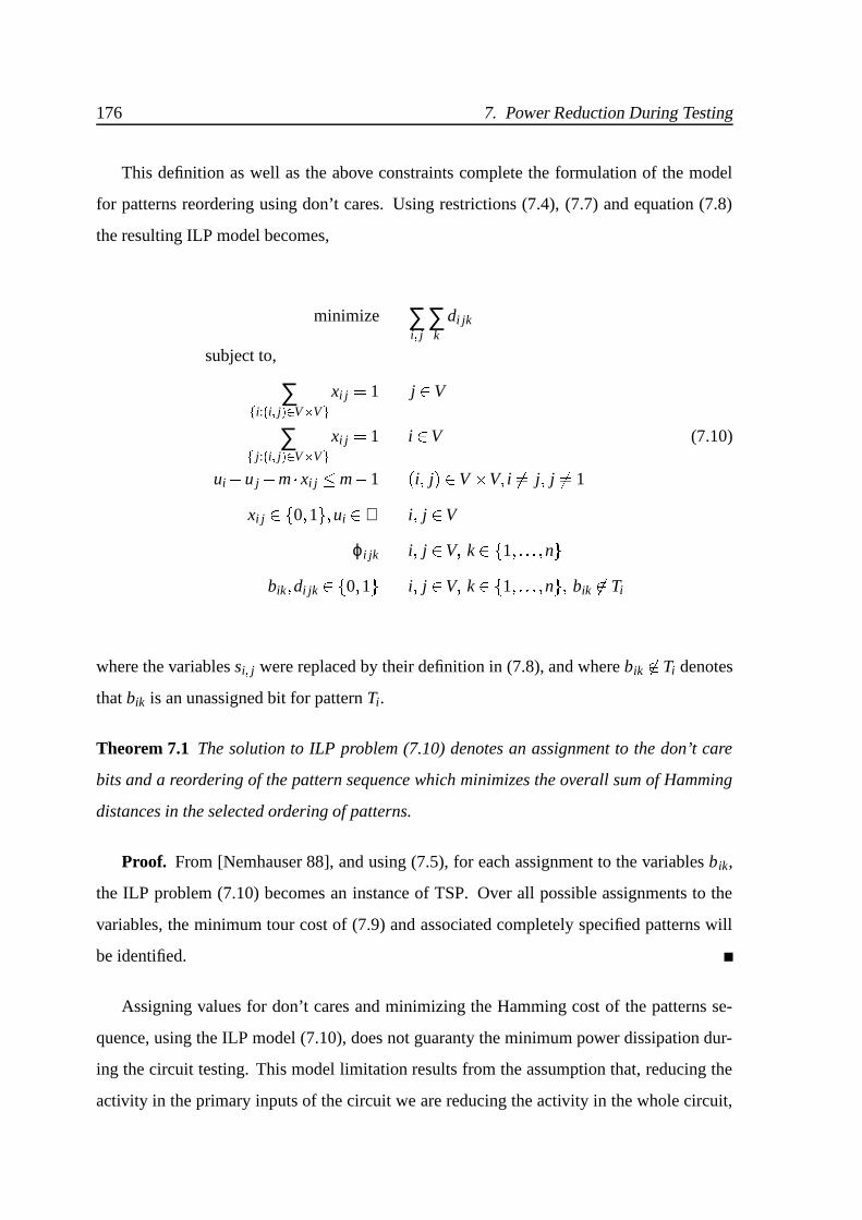
176 7. Power Reduction During Testing
This definition as well as the above constraints complete the formulation of the model
for patterns reordering using don’t cares. Using restrictions (7.4), (7.7) and equation (7.8)
the resulting ILP model becomes,
minimize ∑i j ∑k
di jk
subject to,
∑1 i: 0 i j 2b. V « V 3 xi j 1 j V
∑1 j: 0 i j 2b. V « V 3 xi j 1 i V (7.10)
ui6 u j m xi j 3 m 6 1 i j V " V i j j 1
xi j 0 1 ui ℜ i j V
ϕi jk i j V k 1 n bik di jk 0 1 i j V k 1 n bik
Ti
where the variables si j were replaced by their definition in (7.8), and where bik Ti denotes
that bik is an unassigned bit for pattern Ti.
Theorem 7.1 The solution to ILP problem (7.10) denotes an assignment to the don’t care
bits and a reordering of the pattern sequence which minimizes the overall sum of Hamming
distances in the selected ordering of patterns.
Proof. From [Nemhauser 88], and using (7.5), for each assignment to the variables bik,
the ILP problem (7.10) becomes an instance of TSP. Over all possible assignments to the
variables, the minimum tour cost of (7.9) and associated completely specified patterns will
be identified.
Assigning values for don’t cares and minimizing the Hamming cost of the patterns se-
quence, using the ILP model (7.10), does not guaranty the minimum power dissipation dur-
ing the circuit testing. This model limitation results from the assumption that, reducing the
activity in the primary inputs of the circuit we are reducing the activity in the whole circuit,

7.5 Power Reduction Algorithms 177
and consequently the power dissipated. Although, this is true for most of the typical cir-
cuits, as shown by the results presented in Section 7.6, there exist circuits for which these
parameters may not be correlated.
The proposed model denotes a complex integer optimization problem, clearly no easier
than TSP. Consequently, and in order to evaluate the practical usefulness of pattern sequence
reordering in the presence of don’t cares, we propose in the next section different heuristic
algorithms for computing approximated solutions to the pattern reordering problem. As will
be empirically illustrated in Section 7.6, don’t cares can actually be particularly useful for
minimizing the Hamming cost of pattern sequences.
7.5 Power Reduction Algorithms
As mentioned in Section 7.3.1, for completely specified test patterns, the straightforward
representation of the power reduction problem as an instance of the TSP problem immedi-
ately yields a wealth of approximation algorithms [Johnson 96]. Our approach is to modify
an existing approximation algorithm for the TSP instead of solving the model proposed in
the previous section with an ILP solver. We chose to adapt the 2-Opt local search approxi-
mation algorithm for the TSP [Johnson 96]. The algorithm modification to use incompletely
specified patterns is explained below. Before, we describe the overall power reduction algo-
rithm, for pattern reordering with don’t cares. Figure 7.3 presents the block diagram of the
resulting power reduction algorithm that is organized as follows:
1. Use a dedicated algorithm for computing a test set where each test pattern contains
don’t cares. Either MTP (from Chapter 5) or ATALANTA [Lee 93] or any other ATPG
that generates test patterns with don’t cares can be used.
2. Apply an heuristic procedure for identifying an initial tour. Several different heuris-
tics have been implemented and are described below.
3. Use the modified 2-Opt local-search approximation algorithm for the TSP to reorder
the test patterns. Repeat this step while the tour cost can be reduced.
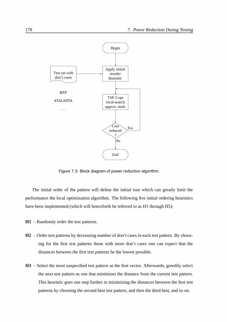
178 7. Power Reduction During Testing
Apply initialreorder
heuristic
TSP 2-optlocal-searchapprox. mod.
Costreduced
?
Begin
End
No
Test set withdon’t cares
MTP
ATALANTA
Yes
. . .
Figure 7.3: Block diagram of power reduction algorithm.
The initial order of the pattern will define the initial tour which can greatly limit the
performance the local optimization algorithm. The following five initial ordering heuristics
have been implemented (which will henceforth be referred to as H1 through H5):
H1 – Randomly order the test patterns.
H2 – Order test patterns by decreasing number of don’t cares in each test pattern. By choos-
ing for the first test patterns those with more don’t cares one can expect that the
distances between the first test patterns be the lowest possible.
H3 – Select the most unspecified test pattern as the first vector. Afterwards, greedily select
the next test pattern as one that minimizes the distance from the current test pattern.
This heuristic goes one step further in minimizing the distances between the first test
patterns by choosing the second best test pattern, and then the third best, and so on.

7.5 Power Reduction Algorithms 179
H4 – In this heuristic for each bit position the don’t care bits are set to the values that occurs
more often for that bit. By using this method the test patterns are expected to become
more similar between each other. Next the test patterns are ordered to approximate
the Gray coding. This approach attempts to order the test patterns in such a way that
the average distances between test patterns is minimized.
H5 – This last heuristic sets the don’t cares in the same manner in the heuristic 4. Af-
terwards, with all the test patterns temporarily specified, the Christofides TSP ap-
proximation algorithm is used for defining the initial tour [Christofides 76]. (A brief
explanation of this algorithm can be found in Appendix C.) This heuristic permits
using a TSP approximation algorithm in a tour where the test patterns are expected to
be similar to each other.
The class of locally optimization algorithms for TSP in which 2-Opt fits are based on
operations that convert one tour into another. Given a initial feasible tour, the algorithm
repeatedly performs operations (i. e. exchanges or moves), so long as each one reduces the
length of the current tour, until a tour is reached for which no operation yields an improve-
ment. The move carried out by the 2-Opt algorithm consists of deleting two edges, thus
breaking the tour into two paths, and then reconnects those paths in the other possible way
to create a unique tour. Figure 7.4 presents a move carried by the 2-Opt algorithm in a set of
eight test patterns.
Therefore, after having the initial tour of the test patterns, obtained by one of the previews
heuristics H1 through H5, the following modified 2-Opt is applied [Johnson 96]:
1. Evaluate the initial tour cost by specifying the don’t care bits which minimize the
distance between consecutive test patterns.
2. Reverse the action taken in Step 1 to get the original test patterns with don’t cares.
3. Apply a 2-Opt move for every edge in the graph. This means that for every pair of test
patterns (Ti and Tj), cut the link between those test patterns and the next ones (Ti 5 1
and Tj 5 1), and link Ti with Tj and Ti 5 1 with Tj 5 1. For this new ordering obtain the
tour cost as in Step 1.

180 7. Power Reduction During Testing
PSfrag replacements
T1T1
T2T2
T3T3
T4T4 T5T5
T6T6
T7T7
T8T8
TiTi
Ti 5 1Ti 5 1TjTj
Tj 5 1Tj 5 1
(a) (b)
Figure 7.4: A 2-Opt move: (a) orginal tour and (b) resulting tour.
4. If the lowest tour cost found in Step 3 is lower than the initial tour cost then keep
the order for that lowest tour cost and repeat Step 1 for that ordering. Otherwise the
algorithm terminates.
Finally, the test sequence that will be used for circuit testing, and which will be provided
to the power estimator of SIS [Sentovich 92], is the result of the modified 2-Opt, with the
don’t care bits specified in such a way that the Hamming distance between consecutive test
patterns is minimized.
7.6 Experimental Results
This section includes results of applying the algorithm described in the previous section
to the IWLS benchmark circuits [IWLS 89] and to the ISCAS’85 benchmark circuits [Brglez 85].
The ATPG tool ATALANTA [Lee 93] was used on all the experiments. As mentioned before
ATALANTA allows the generation of test patterns with don’t cares and was used to generate
both completely and incompletely specified test patterns. The MTP tool (from Chapter 5) was
used in the IWLS benchmark circuits to illustrate that, in general, minimizing the number of
specified bits yields larger power reductions, even if the number of vectors increase.
The experimental procedure consisted of first generating a set of completely specified
7.6 Experimental Results 181
test patterns with ATALANTA and subsequently reordering them such that the Hamming cost
was minimized. For this minimization procedure, the Christofides approximation algorithm
was used (as the initial tour finder) with the 2-Opt local optimization algorithm. This input
pattern sequence is then used to compute the reference values for the Hamming costs and
power consumption used in subsequent comparisons.
Afterwards, the set of incompletely specified test patterns was generated. The algorithm
described in the previous section was used to generate the best ordering and don’t-care as-
signment for the different initial ordering heuristics proposed.
7.6.1 IWLS Benchmarks
We first present in Table 7.1 results for the IWLS benchmark circuits on the reduction
of the Hamming cost by exploiting the don’t cares in the incompletely specified set of test
patterns (generated by ATALANTA), which is the figure of merit that we are directly targeting.
For each of the different heuristics, the percentage savings relative to the optimal sequence
of completely specified pattern sequence is shown. It can be observed that for many of the
examples significant reductions in the Hamming cost are obtained. These savings can vary
widely from circuit to circuit, yet the difference between heuristics is not large, with a slight
advantage for heuristic H3.
Still in Table 7.1 we give the CPU time in seconds used by the ordering and assign-
ment algorithm under the different heuristics on a Sun Ultra I with 384MB of main memory.
These values are reasonably small, confirming the efficiency of the proposed technique, be-
ing heuristics H3 and H5 the least time consuming.
The power reduction results obtained for the same circuits and using the same test vectors
are shown in Table 7.2. The columns labeled completely specified indicate the percentage
power reductions that result from ordering a sequence of completely specified test patterns,
and the number of computed test patterns (#TP). The columns labeled incompletely speci-
fied indicate the power reductions from exploiting the don’t cares in incompletely specified
test patterns over an already ordered sequence of completely specified test patterns for each

182 7. Power Reduction During Testing
Circuit H1 H2 H3 H4 H5
% CPU % CPU % CPU % CPU % CPU
9symml 7.7 17.3 10.5 17.9 16.1 2.0 14.7 18.4 14.7 4.1
alu4 24.3 153.1 22.7 156.9 30.5 16.2 22.7 129.0 29.0 47.6
cht 59.0 0.0 60.3 0.0 59.7 0.0 59.0 0.0 59.0 0.0
cm138a 18.0 0.0 16.0 0.0 16.0 0.0 16.0 0.0 14.0 0.0
cm150a 61.4 1.4 65.5 1.5 65.5 0.2 64.7 1.0 71.3 1.0
cm163a 40.5 0.0 48.6 0.0 43.2 0.0 45.9 0.0 48.6 0.0
cmb 32.6 0.1 32.6 0.0 32.6 0.0 32.6 0.0 32.6 0.0
comp 67.2 12.3 67.9 13.0 70.7 4.8 67.2 12.5 65.8 5.0
comp16 50.8 131.0 59.3 98.7 61.7 11.8 50.3 98.1 60.7 22.1
cordic 56.2 3.9 61.1 3.1 61.1 0.7 59.2 3.5 61.1 0.7
cu 48.3 0.2 48.3 0.1 52.6 0.1 50.5 0.1 50.5 0.0
majority 14.0 0.0 16.0 0.0 14.0 0.0 16.0 0.0 14.0 0.0
misex1 43.4 0.0 39.1 0.0 47.8 0.0 47.8 0.0 43.4 0.0
misex2 72.9 1.6 96.0 1.5 96.0 0.4 76.5 1.9 74.4 0.7
misex3 27.0 815.1 24.1 744.5 35.8 67.6 25.8 667.7 28.7 309.2
mux 67.9 1.2 66.2 1.3 69.5 0.5 68.7 1.2 67.9 0.6
pcle 47.6 0.0 49.5 0.0 47.6 0.0 49.5 0.0 49.5 0.0
pcler8 59.7 0.2 58.7 0.2 59.7 0.1 60.8 0.2 61.9 0.1
term1 71.3 3.7 73.0 4.2 74.7 2.3 74.4 4.5 74.4 2.5
too large 57.7 817.1 60.8 745.8 63.3 217.5 58.6 604.9 63.3 335.5
unreg 64.1 0.0 63.2 0.0 63.2 0.0 64.1 0.0 63.2 0.0
AVERAGE 47.2 93.2 49.5 85.2 51.5 15.4 48.8 73.5 49.9 34.7
Table 7.1: Hamming cost reduction and CPU times for the IWLS benchmark circuits.
heuristic1. In all cases a power estimator tool integrated in SIS [Sentovich 92] was used for
1The absolute value of power reduction percentage can be easily calculated using the table values.

7.6 Experimental Results 183
estimating the actual power dissipation from applying the test sequences [Costa 97].
As can be readily concluded, large power savings ranging from 30% to 60% are achieved
in most cases. This is particularly significant since these results measure the percentage
power savings over the already ordered sequence of test patterns. Finally, we note that the
number of test patterns (#TP) does not change significantly from completely specified to
incompletely specified test patterns. In addition, the results from Table 7.1 and Table 7.2
indicate that the measured reduction in power dissipation correlates well in most circuits
with the achieved reduction in Hamming cost.
Table 7.3 presents the power reductions obtained for incompletely specified patterns gen-
erated by the MTP ATPG tool (with fault simulation and reverse fault simulation but no com-
paction). Thus, the number of don’t cares in each test pattern increases, so as the number
of computed test patterns for the same fault coverage (100%). This boost the number of
available combinations for selecting the low cost tour and assigning of the don’t care bits.
Therefore, Table 7.3 shows that in most cases larger power savings are achieved with these
patterns, than with the ones generated with ATALANTA. In most cases the power reduction
ranges from 40% to 80%. In some few cases (9symml, cm138a, cm150a, comp and majority)
the power reduction is less than expected (when compared with the vectors from ATALANTA),
because even with an “optimal” order and bit assignment the selected test sequence will ac-
tually dissipate more power. This kind of results are somehow expected, and they may be
caused by longer test sequences and/or resulting from the “unconstrain” selection of the test
vectors by the ATPG, which are “randomly” choose regarding to power dissipation.

184 7. Power Reduction During Testing
Completely specified Incompletely specified
(ordered vs. unordered) versus ordered completely specified
Circuit [ATALANTA ATPG] [ATALANTA ATPG]
#TP % power #TP % power reduction
reduction H1 H2 H3 H4 H5
9symml 78 43.9 80 3.8 7.2 15.3 11.1 17.1
alu4 100 29.0 128 12.2 11.7 18.3 13.7 20.4
cht 17 5.6 10 25.3 27.9 24.7 17.9 23.0
cm138a 12 36.3 12 20.9 20.7 11.0 16.2 17.5
cm150a 34 16.5 39 38.6 46.2 53.6 42.4 45.3
cm163a 15 15.6 14 31.2 34.7 40.0 35.4 42.7
cmb 30 43.2 27 16.9 17.7 21.9 13.8 15.1
comp 56 27.1 60 57.0 56.9 60.6 58.7 57.7
comp16 72 38.9 99 40.6 47.6 44.2 46.6 42.3
cordic 43 36.6 47 49.3 56.2 61.5 54.0 59.4
cu 27 35.6 26 23.4 34.3 36.4 13.1 30.3
majority 11 36.1 11 9.6 15.9 5.1 10.9 4.6
misex1 18 14.3 17 36.2 26.5 24.9 26.7 33.0
misex2 47 20.5 37 41.7 48.7 52.6 52.5 51.6
misex3 154 38.3 178 21.0 24.6 27.9 19.1 24.5
mux 35 20.5 38 28.7 31.2 36.9 41.4 32.0
pcle 17 16.6 20 28.1 37.1 47.2 31.2 42.7
pcler8 19 20.4 21 35.4 23.7 43.2 27.5 37.8
term1 43 14.4 43 43.6 49.5 47.2 39.6 46.9
too large 103 32.1 146 36.1 41.2 49.9 42.1 46.3
unreg 15 15.8 10 12.4 12.5 12.0 11.2 17.2
Table 7.2: Power reduction results for the IWLS benchmarks with vectors generated by
ATALANTA.

7.6 Experimental Results 185
Completely specified Incompletely specified
(ordered vs. unordered) versus ordered completely specified
Circuit [ATALANTA ATPG] [MTP ATPG]
#TP % power #TP % power reduction
reduction H1 H2 H3 H4 H5
9symml 78 43.9 83 4.8 8.0 13.5 2.6 11.2
alu4 100 29.0 217 33.2 33.0 52.7 38.1 46.1
cht 17 5.6 184 83.0 89.8 90.7 90.0 91.4
cm138a 12 36.3 12 0.5 0.5 13.5 17.8 8.1
cm150a 34 16.5 43 36.9 49.6 49.7 34.7 59.9
cm163a 15 15.6 35 70.3 73.0 76.4 73.4 71.2
cmb 30 43.2 30 24.7 22.7 26.5 30.2 21.9
comp 56 27.1 70 53.7 54.7 57.2 52.5 58.4
comp16 72 38.9 138 55.2 56.6 56.1 48.8 54.1
cordic 43 36.6 48 60.0 55.6 65.8 60.1 60.5
cu 27 35.6 36 44.2 47.9 46.6 42.8 46.7
majority 11 36.1 11 10.1 -13.9 -3.0 9.6 6.3
misex1 18 14.3 21 39.8 29.1 45.1 41.7 44.6
misex2 47 20.5 69 66.7 68.5 66.9 69.0 70.1
misex3 154 38.3 247 36.3 34.9 45.0 30.5 39.7
mux 35 20.5 42 40.0 48.9 47.5 38.2 37.7
pcle 17 16.6 46 67.3 76.2 77.2 73.5 73.0
pcler8 19 20.4 65 74.1 80.8 77.2 75.1 78.2
term1 43 14.4 109 69.9 76.0 74.0 74.2 73.1
too large 103 32.1 194 52.5 53.0 64.4 53.8 60.4
unreg 15 15.8 116 78.4 86.2 88.3 81.2 87.6
Table 7.3: Power reduction results for the IWLS benchmarks with vectors generated by MTP.

186 7. Power Reduction During Testing
7.6.2 ISCAS Benchmarks
The results in the previous section validate the proposed approach for reducing power
dissipation for medium-size circuits. We now apply the power reduction procedure to the
ISCAS’85 benchmark circuits with test patterns generated by ATALANTA. The results are
shown in Table 7.4. As can be concluded, once again, large power savings can be obtained
by generating test patterns with don’t cares, reordering the test sets and specifying the unas-
signed bits so that the dissipated power is minimized. From Table 7.4, we can conclude that
with specified test patterns, the power savings from reordering the test patterns range from
10% to 30%. In addition, after generating test patterns with don’t cares we obtain, over the
already ordered (but completely specified) test sequence, power savings that range from 10%
to 70%. Moreover, for the majority of benchmarks the power savings are between 40% and
60%. Consequently, we can conclude that test pattern reordering in the presence of don’t
cares leads to large power savings over already ordered test sequences.
Furthermore, we noticed that the percentage of power savings in general increases as
the size of the circuit and number of test patterns increases. Hence, for large circuits we
expect the proposed power reduction algorithm to lead to similar or greater power savings.
Regarding the heuristics proposed in Section 7.5 for constructing the initial tour, the results
do not identify a clear best heuristic, even though the greedy heuristic H3 performs better
in most cases. Finally, these experimental results clearly indicate that exploiting don’t cares
in sequences of test patterns may prove extremely useful whenever power reduction during
testing is the main objective.
For the ISCAS’85 benchmarks we noticed that the proposed (and non-optimized) 2-Opt
algorithm would take a couple of hours of CPU time for the examples with a larger number
of test patterns, and would take more than 24 hours of CPU time for C7552. As a result,
we restricted the 2-Opt algorithm so that only 500 random links were examined at each
iteration of the 2-Opt algorithm (instead of a number that is quadratic in the number of test
patterns). Using this restrained 2-Opt algorithm all the ISCAS’85 benchmarks ran in less
than ten minutes. The results obtained are shown in Table 7.5. As can be concluded, for
the benchmarks with a larger number of test patterns, the new results can be significantly
worse, thus indicating a tradeoff between the computational effort spent with the reordering

7.6 Experimental Results 187
Completely specified Incompletely specified
(ordered vs. unordered) versus ordered completely specified
Circuit [ATALANTA ATPG] [ATALANTA ATPG]
#TP % power #TP % power reduction
reduction H1 H2 H3 H4 H5
C432 58 16.9 75 36.7 48.6 43.5 41.3 43.0
C499 60 28.9 61 18.3 14.8 17.4 18.5 15.9
C880 51 10.4 79 52.1 46.8 44.9 44.9 54.2
C1355 94 30.5 96 9.7 7.8 10.8 11.4 10.7
C1908 128 27.4 175 44.8 45.2 50.3 44.7 50.8
C2670 117 14.2 156 68.0 68.5 68.7 66.2 69.4
C3540 159 18.7 253 30.7 33.6 44.2 33.9 47.4
C5315 116 11.0 158 50.1 49.9 52.9 50.7 53.6
C6288 25 18.6 54 55.6 57.7 57.5 57.1 53.9
Table 7.4: Power reduction results for the ISCAS’85 benchmarks.
algorithm and the attained power savings.
Note that, the results for the ISCAS’85 benchmark circuits with patterns generated by
MTP are not shown, because the number of generated test patterns for each of these circuits
is too large. Thus, running our heuristic algorithm over those patterns will require several
days. Even with the use of the restricted 2-Opt algorithm the number of links to be examined
must be significantly reduced, when compared with the available number of links, so that
a optimized solution is obtained within a predefined time budget (that we choose to be 24
hours). As expected, and already shown, analyzing such a reduced number of links will
produce a less optimized solution. Therefore, comparisons of the achieved power reductions
with the ones obtained using ATALANTA vectors would be expected to be meaningless.

188 7. Power Reduction During Testing
Completely specified Incompletely specified
(ordered vs. unordered) versus ordered completely specified
Circuit [ATALANTA ATPG] [ATALANTA ATPG]
#TP % power #TP % power reduction
reduction H1 H2 H3 H4 H5
C432 58 10.4 75 48.4 45.9 49.0 45.1 51.3
C499 60 30.5 61 5.3 5.9 7.8 5.7 5.1
C880 51 27.4 79 33.5 38.6 49.6 35.5 48.5
C1355 94 14.2 96 58.1 64.5 68.6 63.2 66.9
C1908 128 18.7 175 20.3 21.7 42.4 30.8 43.4
C2670 117 16.9 156 37.2 40.7 44.9 35.2 45.6
C3540 159 28.9 253 13.5 8.1 18.8 14.2 20.1
C5315 116 11.0 158 47.5 45.5 51.2 44.8 51.5
C6288 25 18.6 54 54.0 54.9 55.6 56.3 50.9
C7552 217 15.1 347 39.7 49.6 64.1 52.7 67.8
Table 7.5: Power reduction results for the ISCAS’85 benchmarks with the restricted 2-Opt
algorithm (500 links examined).
7.7 Conclusions
In this chapter we propose a formal optimization model for reducing the Hamming cost
in pattern sequences with unspecified bits. The solution of the model will identify not only
the pattern sequence but also the values of the unspecified bits. Moreover, and due to the
complexity in solving the proposed model, we described a heuristic algorithm for obtaining
approximated solutions. This algorithm is then applied to reducing the power dissipation
during testing by exploiting the order of the patterns and the don’t cares in test pattern se-
quences. We provide experimental evidence that the Hamming cost of a test sequence cor-
relates well with the power dissipated during testing and that exploiting don’t cares in test
sequences can lead to very significant savings in dissipated power. In designs where periodic
testing is required, these power reduction techniques may play a key role in the design of

7.7 Conclusions 189
BIST hardware. Moreover, the use of ATPGs that can generate test sequences with large
number of unspecified bits, as the MTP ATPG proposed in Chapter 5, can play an important
role to achieve considerable power savings. However, for large test sequences there should
be a balance between the aimed power savings and the running time of the algorithm, since
the proposed algorithm has time complexity of O n2 .

190

Chapter 8
Conclusions and Future Research Work
Contents
8.1 Contributions and Conclusions
8.2 Future Research Work
191

192 8. Conclusions and Future Research Work

8.1 Contributions and Conclusions 193
8.1 Contributions and Conclusions
The increasing complexity of the digital circuits integrated in a single chip, with a re-
duced number of I/O pins, is driving the testing of circuits to become a very complex task
and one of the major costs in the integrated circuit industry. Although the research area of
testing has existed for several decades, most problems, in particular optimization problems
in ATPG, have been solved using heuristic approaches.
Discrete algorithms, especially satisfiability search algorithms, have been shown to be a
promising technique to solve decision and optimization problems in many areas of science
and engineering. In particular, the capability to use these algorithms to solve either ATPG
problems and also specific forms of optimization problems, casted as zero-one ILPs, lead us
to propose formal and exact optimization models for ATPG problems.
Therefore, the main contribution of the research work developed in this thesis is the
definition of these formal optimization models for ATPG problems. We considered key opti-
mization problems that directly impact testing time, complexity of BIST and power dissipa-
tion during test. Besides their theoretical interest, the proposed models provide also a formal
basis that can be used to evaluate most heuristic approaches, e.g. by computing optimum
solutions with the formal optimization models, for small-size circuits, and then comparing
how close the heuristic solutions are from those.
For the first time we used a SAT-based algorithm using a branch-and-bound procedure
for optimization. An evaluation of the bsolo tool, that implements this new algorithm, was
performed and showed that bsolo is faster and can solve more zero-one specific classes of
ILP instances than other tools based on satisfiability algorithms or other generic optimization
algorithms. For this reason, we have used the bsolo tool to solve the zero-one ILP instances
for the models proposed in the thesis.
We have proposed a new exact model to find the minimum-size test set for a combina-
tional circuit. To our best knowledge, only two other non-heuristic proposals exist for this
problem. One has a worst-case exponential representation size and the other, that we consid-
ered as the reference model, has a worst-case representation size that is cubic in the number
of nodes of the circuit. The new proposed model also has a worst-case polynomial represen-
194 8. Conclusions and Future Research Work
tation size that is cubic, but we have showed that for typical circuits the resulting size of the
ILP representation is significantly reduced (up to 47% when compared with equivalent in-
stances for the reference model). Moreover, we describe several techniques to further reduce
the size of the new model. However, the size of the resulting ILP instances, for large circuits,
is still too large for practical use. Therefore, we considered an alternative post-generation
method for computing minimal test sets and implemented a tool (MTSC) that uses the set cov-
ering model to compact the test sets. MTSC can be used in conjunction with any ATPG tool
to eliminate vectors from a test set without reducing its fault coverage. Using this test set
compaction tool we studied the effect of ATPG fault simulation in the size of the final test
set. Experimental results indicate that additional test set compaction can be achieved, even
for ATPGs that use heuristics to obtain minimal test sets. Moreover, whenever the goal is a
minimal test set one may consider using efficient ATPG algorithms targeting all faults, i.e.
using a collapsed fault set but without using fault simulation. This increases the size of the
initial test set, but enables the computation of final test sets that are in general smaller than
those obtained when fault simulation is used.
Other contribution of this thesis was the proposal of an extension to existing satisfi-
ability-based ATPG models to compute test patterns with don’t cares. The existing models
and algorithms for generation of test patterns compute, in general, test patterns with more
specified bits than actually needed for detecting a fault. This results from the heuristic nature
of the algorithms and from the use of models which assume only two logic values (0 and
1) when mapping the circuit representation into an algebraic formula. We proposed a new
ATPG satisfiability model that is adequate to directly represent the don’t care values. This
model was cast into an ILP problem to compute test patterns with don’t cares and under the
additional constraint that the number of specified primary input assignments be minimized.
The limitations of the proposed model were presented and its correctness was proved. We de-
veloped an ATPG tool (MTP) that implements this optimization model and used it to illustrate
the applicability of the model by computing minimum size test patterns for the IWLS and
the ISCAS’85 benchmark circuits. We showed that the heuristics used by structural ATPG
algorithms are able to produce test sets with don’t cares but, when the goal is maximizing
the number of don’t care bits, the MTP tool can augment the number of unspecified bit as-

8.1 Contributions and Conclusions 195
signments from the test sets computed by ATPG algorithms. As expected, the improvements
obtained by MTP are limited by the amount of allowed search effort, which directly impacts
the computation time.
We have also derived a new ATPG model targeting the development of a minimal BIST
circuit generator. The most common BIST architectures for test patterns generators are based
on LFSRs. These architectures introduce some area penalty to reduce the testing time with-
out compromising the fault coverage of the circuit. We used a counter-based test generator
architecture that is able to reduce simultaneously the testing time and the test generator area
overhead, guaranteeing a 100% fault coverage. The reduction is as large as the number of
primary inputs that can be declared compatible for testing purposes. The derived ATPG
model uses the previously developed model for test pattern generation with don’t cares with
additional constraints for identifying the maximum number of compatible inputs. This model
was implemented in the MTP-C ATPG tool using a relaxed cost function due to the limitations
imposed by the bsolo optimizer. Despite using this relaxed cost function we showed the ap-
plicability of the model by computing test patterns for the IWLS and ISCAS’85 benchmark
circuits. The resulting test sets exhibit, in general, a larger number of compatible inputs than
the test sets obtained using traditional ATPG algorithms. However, for some circuits, the
final number of bits in the counter of the test pattern generator exceeds 25–30 bits. For those
circuits, additional compression techniques should be considered so that the counter-based
test generator architecture be worthwhile in practice.
Finally, we proposed a model for test pattern sequence reordering and bit assignment
to reduce the power dissipated during circuit testing. As the power dissipation in a circuit
gains importance, for example due to mobile computing, techniques to reduce power dis-
sipated during BIST also become important, in particular for circuits in which testing is
performed periodically. We considered the Hamming distance between pairs of vectors in a
test sequence as a metric for the corresponding power dissipation in a CMOS circuit. The
proposed exact ILP model identifies simultaneously the optimum test pattern sequence and
the don’t care assignment that minimizes the total cost of the Hamming distance. Given the
complexity of the proposed model we implemented an approximation algorithm (using an
heuristic approach) for solving the problem of test pattern reordering with unspecified bits
196 8. Conclusions and Future Research Work
to minimize the power dissipated during test set application. The experimental results for
benchmark circuits confirm that the Hamming cost correlates well with the power dissipated
during testing, and that the existence of don’t cares in the test sequence has a direct impact
in the reduction of the dissipated power.
As a final conclusion, we could say that in this thesis we try to answer to the following
question: is it possible to have formal and exact optimization models for ATPG problems?
Indeed, formal optimization models, based on propositional satisfiability, can be devised for
ATPG problems. But, their use is somehow limited due to the size of the models proposed
or to the computational effort (CPU time) needed to solve each model and to find optimum
solutions. Considering that, in general, solving discrete optimization problems is harder than
solving satisfiability problems, it was not expected that the complexity of ATPG optimization
problems scaled well with the size of the circuits. Observe that while for optimization prob-
lems the whole search tree has to be traversed (explicitly or hopefully implicitly) to compute
a solution, for satisfiability problems any successful traversal suffices to determine a solu-
tion. Therefore, most ATPG problems have been solved using heuristic approaches and we
have ourselves proposed heuristic algorithms for some optimization problems. These heuris-
tics are either new, in the sense that they solve new optimization test problems, or different
approaches to well-known optimization problems. However, because of the inexistence of
formal models until now, it was not possible to compute fully optimized test sets, even if one
was willing to pay a high computational cost. Upholding an expensive test pattern generation
process might actually be desirable when the computational effort and cost to get an optimal
test set, that is done once per circuit, is compensated by the savings obtained in testing the
target circuit millions of times, in the production line and/or on the system. Moreover, using
the proposed satisfiability-based optimization algorithm one may limit the amount of search
to a predefined value and obtain, in a reasonable amount of time, an approximate solution
to the given problem. From our experience this solution is, in general, superior to the one
computed using heuristic approaches.
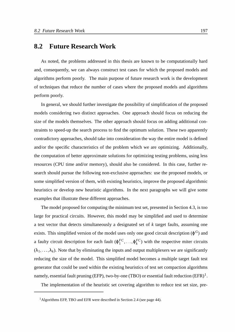
8.2 Future Research Work 197
8.2 Future Research Work
As noted, the problems addressed in this thesis are known to be computationally hard
and, consequently, we can always construct test cases for which the proposed models and
algorithms perform poorly. The main purpose of future research work is the development
of techniques that reduce the number of cases where the proposed models and algorithms
perform poorly.
In general, we should further investigate the possibility of simplification of the proposed
models considering two distinct approaches. One approach should focus on reducing the
size of the models themselves. The other approach should focus on adding additional con-
straints to speed-up the search process to find the optimum solution. These two apparently
contradictory approaches, should take into consideration the way the entire model is defined
and/or the specific characteristics of the problem which we are optimizing. Additionally,
the computation of better approximate solutions for optimizing testing problems, using less
resources (CPU time and/or memory), should also be considered. In this case, further re-
search should pursue the following non-exclusive approaches: use the proposed models, or
some simplified version of them, with existing heuristics, improve the proposed algorithmic
heuristics or develop new heuristic algorithms. In the next paragraphs we will give some
examples that illustrate these different approaches.
The model proposed for computing the minimum test set, presented in Section 4.3, is too
large for practical circuits. However, this model may be simplified and used to determine
a test vector that detects simultaneously a designated set of k target faults, assuming one
exists. This simplified version of the model uses only one good circuit description (ϕG) and
a faulty circuit description for each fault (ϕFC1 ϕFC
k ) with the respective miter circuits
(λ1 λk). Note that by eliminating the inputs and output multiplexers we are significantly
reducing the size of the model. This simplified model becomes a multiple target fault test
generator that could be used within the existing heuristics of test set compaction algorithms
namely, essential fault pruning (EFP), two-by-one (TBO) or essential fault reduction (EFR)1.
The implementation of the heuristic set covering algorithm to reduce test set size, pre-
1Algorithms EFP, TBO and EFR were described in Section 2.4 (see page 44).

198 8. Conclusions and Future Research Work
sented in Section 4.4.1, has the capability to use test set partitions to reduce the size and
complexity of the problem. Additional research should be performed to identify the best
set of partitions regarding their size and the test patterns to be included in each partition
considering the circuit structure and the faults detected by each test vector.
In Section 6.4 we proposed a solution for the identification of minimal BIST test pattern
generators. The proposed greedy algorithm may be enhanced with a heuristic pre-processing
phase which should sort the fault list to increase the number of compatibility relations and/or
reduce the total computation time. One alternative solution to identify the maximum number
of compatibility classes might consider using the proposed model as a post-generation width
compressor. In this approach the test set is generated using a generic ATPG, and then, a
compatibility graph is built for identifying the vectors responsible for each compatibility vi-
olation. If, using the proposed model, we can replace these vectors with new ones that detect
the same essential faults and simultaneously reduce the number of compatibility classes, we
determine a smaller BIST test pattern generator.
In any case, to further reduce the width of the counter in the test generator circuit we
should consider the incorporation in the model of new types of compatibility. However,
these new types should be restricted to simple logic functions (such as OR, AND, XOR
or other 2-input logic functions), so that the area of the decoder circuit does not increase
significantly.
A comparative study of the fault coverage achieved by pseudo-random testing using tra-
ditional BIST architectures based on simple LFSRs, and the architecture used should also
be done. Special attention should be given for circuits in which some compatible inputs
are identified but the final width of the counter exceeds 25–30 bits, thus not all input com-
binations can be applied to the CUT. In general, we should study how the existing BIST
techniques (e.g. pseudo-exhaustive, LFSR and seed selection, etc) can take advantage of the
input compatibility identified by the proposed model, regarding fault coverage, testing time
and total BIST circuit area.
The algorithmic solution proposed for reordering test patterns with don’t care assign-
ment, in Section 7.5, is limited by the size of the test set because its time complexity is
O n2 . As future research work we intend to develop a more flexible configuration of the

8.2 Future Research Work 199
local search optimization algorithm (2-opt), that will permit to control the number of iter-
ations implemented by the algorithm and, consequently, its execution time and the amount
of power savings. Additional research work involves experimenting with the proposed for-
mal optimization model with the goal of estimating the gains obtained with respect to the
heuristic algorithm. The impact of reordered test sequences in the resulting BIST logic area
must also be evaluated, even though power and not area is currently the key metric for some
applications.
Finally, a long-term objective of this work is the integration of the proposed models and
algorithms in a complete testing environment, thus enabling a framework for faster devel-
opment of new optimization models and algorithms for specific target applications. In this
environment we intend to support different SAT and ILP solvers, in particular, an extend
version of bsolo that accepts a generic linear cost function. Additional, we should consider
using dedicated hardware to implement and accelerate the SAT/ILP solver algorithms. An
attractive solution to this problem is to use reconfigurable hardware, based on Field Pro-
grammable Gate Array (FPGA) architectures, and investigate its customization to a specific
algorithm and optimization model. In this environment, we also plan to read circuit descrip-
tions using different hardware description languages, such as blif, VHDL and Verilog. In
addition, this framework could promote studying algorithms for the synthesis of BIST test
pattern generators optimized according to some cost function. The parameters selected for
the cost function should consider the fault coverage, testing time, power dissipation, cir-
cuit area, among others. Other CAD problems, not directly related with test, could also be
considered for optimization within the proposed framework with further research and devel-
opment of new specific ILP/SAT models for those problems (e.g. schedule and allocation
tasks in high level synthesis [Flores 97]).

200

Appendix A
Model Validation and Limitations
In order to establish the validity of the proposed model for the computation of minimum
size test patterns, we must first formally define the notion of test pattern minimization. This
notion in tightly related with the way lines are justified to the primary inputs and the way
error signals propagate from the fault site to the primary outputs. Before proving the validity
of the model we will introduce some useful definitions which are based on the combinational
circuit definitions presented in Section 2.2 (see page 23).
Definition A.1 (Specialization/Cover) Given incompletely specified test patterns T x1 x2 xn
and T ª x 1 x 2 x n , we say that T specializes T provided there exists at least one vari-
able xi, i 1 n , such that xi X in T and x i 0 1 in T , meaning that input i is
unspecified in T but specified in T . Moreover, any specified assignment in T is also a speci-
fied assignment in T with the same value, i.e. xi v ) v 0 1 0 x i v. Conversely, we
say that T covers T .Definition A.2 (S-Path) For a fault f a s-path (i.e. a sensitization path) denotes a sequence
of nodes y1 y2 yk , connecting the fault site y1 to a primary output yk PO such that
the sensitization variable ySj 1 j 7 1 k . For a given fault f and a test pattern T , the
set of all s-paths is denoted by PS T f .Definition A.3 (S-Irrelevant assignment) We say that an assignment xi v is s-irrelevant
(i.e. sensitization irrelevant) with respect to a fault f and a test pattern T , if and only if,
201
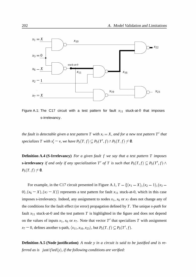
202 A. Model Validation and Limitations
x10
x19
x22
x23
x16
x2 1
x7 X
x1 X
x3 0
x6 Xx11
stuck-at-0
Figure A.1: The C17 circuit with a test pattern for fault x11 stuck-at-0 that imposes
s-irrelevancy.
the fault is detectable given a test pattern T with xi X, and for a new test pattern T that
specializes T with x i v, we have PS T f PS T f 9) PS T f /0.
Definition A.4 (S-Irrelevancy) For a given fault f we say that a test pattern T imposes
s-irrelevancy if and only if any specialization T of T is such that PS T f PS T f =)PS T f /0.
For example, in the C17 circuit presented in Figure A.1, T x1 X x2 1 x3 0 x6 X x7 X represents a test pattern for fault x11 stuck-at-0, which in this case
imposes s-irrelevancy. Indeed, any assignment to nodes x1, x6 or x7 does not change any of
the conditions for the fault effect (or error) propagation defined by T . The unique s-path for
fault x11 stuck-at-0 and the test pattern T is highlighted in the figure and does not depend
on the values of inputs x1, x6 or x7. Note that vector T that specializes T with assignment
x7 0, defines another s-path, x11 x16 x23 , but PS T f PS T f .
Definition A.5 (Node justification) A node y in a circuit is said to be justified and is re-
ferred as is / justi f ied y , if the following conditions are verified:

203
x10
x19
x22
x23
x16
x2 1
x7 X
x1 X
x3 0
x6 Xx11
stuck-at-0
Figure A.2: The C17 circuit with a test pattern for fault x11 stuck-at-0 that imposes
j-irrelevancy.
is / justi f ied y ! y X
y PI
y fy I y ) ý
z j . I 0 y 2 is / justi f ied z j (A.1)
where I y denotes the fanin nodes of y and fy I y denotes the output logic value of the
nodes that drive y calculated from the values currently assigned to the fanin nodes of y.
Definition A.6 (J-Path) For a fault f in a circuit where all nodes are justified, i.e.ý
xi . VC
is / justi f ied xi , a j-path (i.e. justification path) denotes the sequence of nodes y1 y2 yk
connecting node y1 to a primary input yk PI such that y j
X and ySj 0, for j 1 k .
For a given fault f and a test pattern T , the set of all j-paths is denoted by PJ T f .Definition A.7 (J-Irrelevancy) For a given fault f we say that a test patterns T imposes
j-irrelevancy if and only if any specialization T of T is such that PJ T f PJ T f =)PJ T f /0.
Similarly to the definition of s-irrelevancy, which states that any specialization of a test
pattern does not modify the error propagation path, the j-irrelevancy definition enunciates

204 A. Model Validation and Limitations
that any specialization of a test pattern does not change the existent justification paths. Fig-
ure A.2 shows the C17 circuit with a test pattern that detects the fault x11 stuck-at-0 and in
which all nodes of circuit are justified. The existent j-paths for this test pattern are high-
lighted and any specialization does not alter these paths, although new ones might appear.
Definition A.8 (SJ-Irrelevancy) For a given fault f we say a test pattern T imposes sj-
irrelevancy if and only if T imposes both s-irrelevancy and j-irrelevancy.
The above definitions basically allow us to introduce the following definition of minimum
size test pattern.
Definition A.9 (Size of a test pattern) Let T be a test pattern, we define the size of T, = T = ,
as the number of specified assignments in T , i.e. = T =ö?>>>,t xi v s t
i 7 1 n ) v 0 1 . >>> .Definition A.10 (Minimum-size test pattern) Let @Tf be the set of all test patterns which
detect a given fault f . Let T @Tf be a test pattern that imposes sj-irrelevancy and T @Tf
be any other test pattern which imposes sj-irrelevancy, such that = T = 3 = T A= . In such a
situation, T is said to be a minimum-size test pattern (with respect to sj-irrelevancy).
As the previous definition implies, in general there may be smaller test patterns which do
not impose s-irrelevancy or j-irrelevancy (or both). An example of a test patterns that does
not impose s-irrelevancy was analyzed in the Section 5.4. Figure A.3 presents a circuit for
which the test pattern T s X v 1 detects the fault stuck-at-0 on node out, but for
which no j-irrelevancy is imposed.
In the remainder of this appendix we show that the proposed optimization model can
indeed be used for computing minimum-size test patterns. The sequence of formal results
basically shows that any implied good and faulty circuit node assignments, due to a given test
pattern T , will not be modified by any specialization of T . This is particularly relevant for
path sensitization and line justification, because it ensures that any computed test pattern
T with unspecified assignments that detects a given fault f , still detects that same fault
if some of the unspecified assignments of T become specified. Thus T is a test for the
fault and implicitly represents a set of tests for the same fault (i.e. all of its specializations).

205
out
stuck-at-0G3
G2
G1G0
s X
v 1
Figure A.3: Minimum-size test pattern for which no justification path is needed.
We conclude by showing that any solution to the proposed optimization model (5.13) (see
page 128) must be of minimum size.
Lemma A.1 Let ϕGu be a CNF formula for a circuit and let T be an assignment to the
primary inputs such that ϕGu T 1. Let y v, v f 0 1 , be a circuit node assignment
implied by T . In this situation and given any specialization of T , the assignment y v is also
implied.
Proof. Given a gate connected solely to the primary inputs of the circuit, if its output
is specified given T is either because all inputs assume a non-controlling value or because
at least one input assumes a controlling value. (Observe that for NOT and BUFF gates
the analysis is similar.) Clearly, the value of the output of this gate cannot change by any
specialization of T . By induction on the topological level of a circuit, the same reasoning
applies on all gates, and the results follows.
Lemma A.2 Let ϕGu be a CNF formula for a circuit and let T be an assignment to the
primary inputs such that ϕGu T 1, then all circuit nodes in the circuit are justified, i.e.
ýxi . VC
is / justi f ied xi .
Proof. Given a node y which is neither unspecified (y X ) nor a primary input (y 5PI), but for which the assigned value, y v1 and v1 0 1 , is different from the logic
function that drives the node, fy I y v2 and v2 7 0 1 , then we have an inconsistent set
of assignments on the gate that drives y. In this situation, the consistency function of the gate

206 A. Model Validation and Limitations
is false and the clauses in ϕGu that represent this gate are not satisfied. Therefore, ϕG
u could
not be satisfied.
Proposition A.1 Given a fault f and a test pattern T and a circuit node y for which the
sensitization variable is 1, yS 1, then for any specialization of T , yS 1 holds.
Proof. From Lemma A.1 we know that any specified good value of any node in the
circuit cannot change with any specialization of T . Furthermore, the faulty value of a node
is only specified when the good value is also specified, from (5.9) (see page 125). Again
applying Lemma A.1 to the faulty values, we can conclude that a specified faulty value
cannot change with any specialization of T . Finally, since the specified good and the faulty
values cannot change for any specialization of T , then any assignment yS 1 can also not
change.
Corollary A.1 Given a fault f and a test pattern T such that ϕDu T 1, then all nodes in the
circuit are satisfied and any unspecified assignment xi X in T is s-irrelevant with respect
to f . Moreover, test pattern T imposes sj-irrelevancy.
Proof. The proof follows from Lemma A.2 and Proposition A.1.
Proposition A.2 A fault f is detectable if and only if the corresponding CNF formula ϕDu is
satisfiable.
Proof. Let us consider a detectable fault f . It is known that for completely specified test
patterns, ϕD is satisfied if and only if fault f is detectable [Silva 97b]. Since f is detectable
we can always find a completely specified test pattern T for which ϕD is satisfied. Thus, all
nodes are justified and we can identify at least one path connecting the fault site to a primary
output such that for any node y in the path yS 1. Consequently, and by the definition of ϕDu ,
T must also satisfy ϕDu .
Conversely, let us consider an assignment for which ϕDu is satisfiable. This necessarily
implies that all nodes are justified and that at least one primary output y for which yS 1
exits. By construction, the value of the good variable for every node in at least one path from
the fault site to primary output y must be specified, and such that for each such node the good
207
value differs from the faulty value. Given that T imposes s-irrelevancy (from Corollary A.1),
then any complete specialization of T still satisfies ϕDu . Considering the reverse mapping
to the original set of variables, then ϕD is also satisfied and from [Silva 97b] the fault f is
detected.
Corollary A.2 Given a fault f and a test pattern T such that ϕDu T 1 , then the fault effect
is observable on at least one primary output and a s-path exists from the fault site to that
primary output.
Proof. Since ϕDu T 1 , then ϕR
u T 1. Thus we have a primary output y such that
yS 1. Consequently, yG yF ) yG 0 1 , and so the fault effect is observable on primary
output y. Note also that a gate whose output is sensitized has at least one input sensitized,
apart from the fault site. Therefore, we can always identify a path, the s-path, from the output
node y to the fault site z, where by definition we have zS 1 due to the fault.
Proposition A.3 Given a fault f , the solution of ILP (5.13) is a minimum-size test pattern
with respect to sj-irrelevancy.
Proof. From Proposition A.2 we know that ϕDu T 1 if and only if the fault is detected
given T . Hence the constraints of the ILP (5.13) are only satisfied for test patterns detecting
the fault. Suppose now that T is the computed solution of (5.13) and suppose further that
there exists T such that T also detects the fault and = T A= B= T = . However, since T is a test
for the fault, it also satisfies the constraints of (5.13) due to Proposition A.2, and so it would
be a better solution than the computed solution of the ILP; a contradiction.

208

Appendix B
Subtours Elimination Proof
In this appendix we will prove that the constraints imposed in equations (7.4) and (7.10)
(see pages 174 and 176, respectively) will exclude any subtour from the solution, without
eliminating valid solutions (complete tours).
Let us consider a graph G V E , where V denotes a finite set of m vertices and E a
binary relation on V that represents the edges between the vertices. A tour or a cycle on
a graph is a set of distinct vertices v1 v2 vk v1 such that there exists an edge in E
for consecutive vertices, (i.e. the pair vi vi 5 1 E V " V ). Note that a tour could also
be determined by the set of edges which link the vertices sequence v1 v2 vk v1 . A
complete tour is a tour where all the m vertices of the graph are included, while a subtour is
a tour where only some vertices are included.
Let xi j denote a Boolean variable such that xi j 1 if vertex vi follows vertex v j in a
selected tour, and xi j 0 otherwise. For the TSP problem we know that if xi j satisfies the
constraints
∑1 i: 0 i j 2 . V « V 3 xi j 1 j V
(B.1)
∑1 j: 0 i j 2 . V « V 3 xi j 1 i V
then the solution is a complete tour or a set of subtours in which all vertices are included.
Proposition B.1 (Subtours Elimination Constraints)
209

210 B. Subtours Elimination Proof
Let X be a tour, identified by its set of edges xi j 1 which satisfies (B.1). The set of con-
straints
ui6 u j m xi j 3 m 6 1 i j V " V i 1 j 1 ui ℜ (B.2)
for some ui ℜ, are only satisfied for complete tours .
Proof. If X satisfies (B.1) and does not represent a complete tour, then X has at least
two subtours, one of which does not contain vertex 1. The sum of (B.2) over the edges of a
subtour X that does not include vertex 1 gives
m ∑0 i j 2 . X xi j 3 X m 6 1 (B.3)
Note that all ui are canceled in any subtour X and xi j is 1 on a subtour, so their sum over the
edges of a subtour is X 4 , which turns the proposition (B.3) to false. Thus, (B.2) excludes all
subtours that do not contain node 1 and hence excludes all solutions that contains subtours.
Now we prove that no complete tours are excluded by constraints (B.2). We will show
that for any complete tour there exists a set of values for ui which satisfies (B.2). One of
these sets is obtained using the assignment ui p, where p is the position (2 3 p 3 m) of
the node i in the tour. Thus, if xi j 0 then, the left side of (B.2) reduces to ui6 u j where
ui and u j are not consecutive, so we always have ui6 u j 3 m 6 2. If xi j 1, which implies
that ui p and u j p 1 for some p, the left side of (B.2) becomes ui6 u j mxi j m 6 1.
Hence the solutions of (B.1) and (B.2) represent only complete tours.
Other type of constraints to eliminate subtours for the TSP problem can be found in [Nemhauser 88].

Appendix C
The Christofides Algorithm
In this appendix we will describe the Christofides algorithm used in the heuristics pro-
posed in Section 7.5 (see page 177) to determine the initial order of the test vectors.
The Christofides algorithm was developed in 1976 by Christofides [Christofides 76]. This
algorithm shows the best results regarding the length of the initial tour for the Travel Sales-
man Problem (TSP) [Johnson 96]. It has been proven that the worst case ratio between the
length of the initial tour and the length of the optimal tour is just 32 , assuming the triangle in-
equality [Cornuejols 76]. This inequality say that the direct path between vertices is always
the shortest route or the lower cost path. Formally, the triangle inequality is defined as
ci j 3 cik ck jý
i j k .^1 1 DCECEC m 3 (C.1)
where ci j is the cost between the two vertices vi and v j, and m is the total number of vertices.
Before describing the Christofides algorithm we will introduce some useful definitions [Aho 74,
Cormen 90].
Definition C.1 (Minimum Spanning Tree) The minimum spanning tree of a undirected graph
G V E , where V denotes a finite set of m vertices and E a binary relation on V that rep-
resents the edges between the vertices, is a subset of edges, T E, that connects all of the
vertices without cycles and minimizes the total cost
C T ∑0 i j 2 . T
ci j (C.2)
211

212 C. The Christofides Algorithm
Definition C.2 (Vertex Degree) The degree of a vertex in an undirected graph is the number
of edges incident on it.
Definition C.3 (Matching) Given a undirected graph G V E , a matching is a subset of
edges M E such that for all vertices v V , at most one edge of M is incident on v.
Definition C.4 (Euler Tour) An Euler tour in a undirected graph G V E is a cycle that
traverses each edge of G exactly only once, although it may visit a vertex more than once.
The Christofides heuristic algorithm proceeds as follows.
1. First, we construct a minimum spanning tree T for the set of edges in the graph. Note
that the length of such tree can not be longer than the optimal solution, since deleting
an edge from the optimal tour yields a spanning tree.
2. Next, we compute a minimum-length matching M on the vertices of odd degree in T .
3. Combining M and T we obtain a connected graph in which every vertex has even
degree. This graph must contain an Euler tour, which can be easily found.
4. A travel salesman tour of no greater cost can then be constructed by traversing this
Euler tour while taking shortcuts to avoid multiple visited cities. Each shortcut re-
places a path between two vertices by a direct edge between them. By the triangle
inequality (C.1) the direct path cannot have greater cost than the paths it replaces.

Bibliography
[Abramovici 90] Miron Abramovici, Melvin A. Breuer, and Arthur D. Friedman. Digital
Systems Testing and Testable Design. IEEE Press, 1990.
[Agrawal 93a] Viswani D. Agrawal, Charles R. Kime, and Kewal K. Saluja. A Tuto-
rial on Built-In Self-Test (Part 1: Principles). IEEE Design & Test of
Computers, pages 73–82, March 1993.
[Agrawal 93b] Viswani D. Agrawal, Charles R. Kime, and Kewal K. Saluja. A Tutorial
on Built-In Self-Test (Part 2: Applications). IEEE Design & Test of
Computers, pages 69–77, June 1993.
[Aho 74] Alfred V. Aho, Jonh E. Hopcroft, and Jeffrey D. Ullman. The De-
sign and Analysis of Computer Algorithms. Addison-Wesley Publish-
ing Company, 1974.
[Aitken 99] Robert C. Aitken. Nanometer Technology Effects on Fault Models for
IC Testing. IEEE Computer, 32(11):46–51, November 1999.
[Akers 58] S. B. Akers. On a Theory of Boolean Functions. Journal of the Society
for Industrial and Applied Mathematics, 7, 1958.
[Akers 78] S. B. Akers. A Logic System for Fault Test Generation. IEEE Trans-
actions on Computers, 25(6):620–630, June 1978.
[Akers 87] S. B. Akers, C. Joseph, and B. Krishnamurthy. On the Role of Inde-
pendent Fault Sets in the Generation of Minimal Test Sets. In Proceed-
213

214 Bibliography
ings of International Test Conference (ITC), pages 1100–1107, August
1987.
[Al-Asaad 98] Hussain Al-Asaad, Jonh P. Hayes, and Briant T. Murrray. Scalable Test
Generators for High-Speed Datapath Circuits. Journal of Electronic
Testing: Theory and Applications, 12:111–125, 1998.
[Barth 95] Peter Barth. A Davis-Putnam Based Enumeration Algorithm for Linear
Pseudo-Boolean Optimization. Technical report, Max-Planck-Institut
Fur Informatik, January 1995.
[Beasley 96] John Edward Beasley. Advances in Linear and Integer Programming.
Oxford University Press, Inc., 1996.
[Berkelaar 92] M. Berkelaar. Unix Manual page of lp solve. Eindhoven University of
Technology, Design Automation Section, [email protected], 1992.
[Brglez 85] F. Brglez and H. Fujiwara. A Neutral List of 10 Combinational Bench-
mark Circuits and a Target Translator in FORTRAN. In Proceedings of
the IEEE International Symposium on Circuits and Systems (ISCAS),
1985.
[Brglez 89] F. Brglez, D. Bryan, and K. Kozminski. Combinational Profiles of Se-
quential Benchmark Circuits. In Proceedings of the IEEE International
Symposium on Circuits and Systems (ISCAS), pages 1929–1934, May
1989.
[Burch 92] R. Burch, F. Najm, P. Yang, and T. Trick. McPower: A Monte Carlo
Approach to Power Estimation. In Proceedings of International Con-
ference on Computer-Aided Design (ICCAD), November 1992.
[Cha 78] C. W. Cha, W. E. Donath, and F. Ozguner. 9-V Algorithm for Test Pat-
tern Generation of Combinational Digital Circuits. IEEE Transactions
on Computers, 27(3):193–200, March 1978.

Bibliography 215
[Chakrabarty 97] Krisnendu Chakrabarty, Brian T. Murray, Jian Liu, and Minyao Zhu.
Test Width Compression for Built-In Self Testing. In Proceedings of
International Test Conference (ITC), November 1997.
[Chakrabarty 98] K. Chakrabarty and B. T. Murray. Design of Built-In Test Generator
Circuits Using Width Compression. IEEE Transactions on Computer-
Aided Design of Integrated Circuits and Systems, 17:1044–1051, Octo-
ber 1998.
[Chakradhar 93] S. T. Chakradhar, V. D. Agrawal, and S. G. Rothweiler. A Transi-
tive Closure Algorithm for Test Generation. IEEE Transactions on
Computer-Aided Design, 12(7):1015–1028, July 1993.
[Chakravarty 94] Sreejit Chakravarty and Vinay Dabholkar. Minimizing Power Dissipa-
tion in Scan Circuits During Test Application. In Proceedings of Inter-
national Workshop on Low Power Design, pages 51–56, April 1994.
[Chandrakasan 92] A. Chandrakasan, T. Sheng, and R. Brodersen. Low Power CMOS
Digital Design. IEEE Journal of Solid State Circuits, 27(4):473–484,
April 1992.
[Chang 95] Jau-Shien Chang and Chen-Shang Lin. Test Set Compaction for Com-
binational Circuits. IEEE Transactions on Computer-Aided Design of
Integrated Circuits and Systems, 14(11):1370–1378, November 1995.
[Chatterjee 95] Mitrajit Chatterjee and Dhiraj K. Pradhan. A Novel Pattern Generator
for Near-Prefect Fault-Coverage. In VLSI Test Symposium (VTS), pages
417–425, 1995.
[Chen 95] Chih-Ang Chen and Sandeep K. Gupta. A Methodology to Design
Efficient BIST Test Pattern Generators. In Proceedings of International
Test Conference (ITC), pages 814–823, 1995.
216 Bibliography
[Christofides 76] N. Christofides. Word-case analysis of a new heuristic for the traveling
salesman problem. Report 338, Carnegi-Mellon University, Pittsburgh,
PA, 1976.
[Cormen 90] T. Cormen, C. Leiserson, and R. Rivest. Introduction to Algorithms.
McGraw Hill e MIT Press, 1990.
[Cornuejols 76] G. Cornuejols and G. L. Nemhauser. Tight Bounds for Christofides
Traveling Salesman Heuristic. Math. Programing, 14:116–121, 1976.
[Costa 97] J. C. Costa, J. C. Monteiro, and S. Devadas. Switching Activity Estima-
tion using Limited Depth Reconvergent Path Analysis. In Proceedings
of the International Symposium on Low Power Design (ISLPD), 1997.
[Costa 98a] Jose C. Costa, Paulo F. Flores, Horacio C. Neto, Jose C. Monteiro,
and Joao P. Marques Silva. Exploiting Don’t Cares in Test Patterns to
Reduce Power During BIST. In IEEE European Test Workshop (ETW),
pages 34–36, May 1998.
[Costa 98b] Jose C. Costa, Paulo F. Flores, Horacio C. Neto, Jose C. Monteiro, and
Joao P. Marques Silva. Power Reduction in BIST by Exploiting Don’t
Cares in Test Patterns. In IEEE/ACM International Workshop on Logic
Synthesis (IWLS), pages 375–386, June 1998.
[Coudert 96] Olivier Coudert. On Solving Covering Problems. In Proceedings of
Design Automation Conference (DAC), June 1996.
[Cox 94] H. Cox and J. Rajski. On Necessary and Nonconflicting Assign-
ments in Algorithmic Test Patterns Generation. IEEE Transactions on
Computer-Aided Design, 13(4):515–530, April 1994.
[Dantzing 51] George B. Dantzing. Programming of Interdependent Activities, II,
Mathematical Model. In T. C. Koopmans, editor, Activity Analysis of
Production and Allocation, pages 19–32. John Wiley & Sons, 1951.

Bibliography 217
[Davis 60] M. Davis and H. Putnam. A Computing Procedure for Quantification
Theory. Journal of the Association for Computing Machinery, 7:201–
215, 1960.
[Devadas 98] Srinivas Devadas and Kurt Keutzer. An Algorithmic Approach to Op-
timizing Fault Coverage for BIST Logic Synthesis. In Proceedings of
International Test Conference (ITC), 1998.
[Dufaza 91] C. Dufaza and G. Canbom. LFSR based Deterministic and Pseudo-
Random Test Pattern Generator Structures. In Proceedings of European
Test Conference (ETC), pages 27–34, 1991.
[Flores 97] Paulo Flores. Sıntese de Alto Nıvel utilizando Programacao Linear
Inteira. Technical report, Relatorio interno INESC/IST, Maio 1997.
[Flores 98a] Paulo F. Flores, Horacio C. Neto, Krishnendu Chakrabarty, and Joao
P. Marques Silva. A Model and Algorithm for Computing Minimum-
Size Test Patterns. In IEEE European Test Workshop (ETW), pages
147–148, May 1998.
[Flores 98b] Paulo F. Flores, Horacio C. Neto, and Joao P. Marques Silva. An Exact
Solution to the Minimum-Size Test Pattern Problem. In Proceedings of
the IEEE International Conference on Computer Design (ICCD), pages
510–515, October 1998.
[Flores 98c] Paulo F. Flores, Horacio C. Neto, and Joao P. Marques Silva. An Exact
Solution to the Minimum-Size Test Pattern Problem. In IEEE/ACM In-
ternational Workshop on Logic Synthesis (IWLS), pages 452–470, June
1998.
[Flores 99a] Paulo Flores, Jose Costa, Horacio Neto, Jose Monteiro, and Joao
Marques-Silva. Assignment and Reordering of Incompletely Specified
Pattern Sequences Targetting Minimum Power Dissipation. In Pro-

218 Bibliography
ceedings of the IEEE/ACM International Conference on VLSI Design
(VLSI), pages 37–41, January 1999.
[Flores 99b] Paulo Flores, Horacio Neto, Krishnendu Chakrabarty, and Joao
Marques-Silva. Test Pattern Generation for Width Compression in
BIST. In Proceedings of the IEEE International Symposium on Cir-
cuits and Systems (ISCAS), volume I, pages 114–118, May 1999.
[Flores 99c] Paulo Flores, Horacio Neto, and Joao Marques-Silva. On Applying Set
Covering Models to Test Set Compaction. In Proceedings of the IEEE
Great Lakes Symposium on VLSI (GLS), March 1999.
[Fourer 00] Robert Fourer. Linear Programming Frequently Asked Questions. Op-
timization Technology Center of Northwestern University and Argonne
National Laboratory, 2000. e-mail: [email protected].
[Fujiwara 82] H. Fujiwara and S. Toida. The Complexity of Fault Detection Problems
for Combinational Logic Circuits. IEEE Transactions on Computers,
31(6):555–560, June 1982.
[Fujiwara 83] H. Fujiwara and T. Shimono. On the Acceleration of Test Generation
Algorithms. IEEE Transactions on Computers, 32(12):1137–1144, De-
cember 1983.
[Garey 79] M. R. Garey and D. S. Johnson. Computers and Intractability: A Guide
to the Theory of NP-Completeness. W. H. Freeman and Company, New
York, 1979.
[Giraldi 90] Jonh Giraldi and Michael L. Bushnell. EST: The New Frontier in Auto-
matic Test-Patterns Generation. In Proceedings of Design Automation
Conference (DAC), pages 667–672, 1990.
[Giraldi 91] J. Giraldi and M. L. Bushnell. Search State Equivalence for Redun-
dancy Identification and Test Generation. In Proceedings of Interna-
tional Test Conference (ITC), pages 184–193, 1991.
Bibliography 219
[Goel 81] P. Goel. An Implicit Enumeration Algorithm to Generate Tests for
Combinational Logic Circuits. IEEE Transactions on Computers,
30(3):215–222, March 1981.
[Golomb 82] S. W. Golomb. Shift Register Sequences. Argean Park Press, Laguna
Hills, Calif., 1982.
[Gomory 58] R. E. Gomory. Outline of an algorithm for integer solutions to linear
programs. Bulletin of the American Mathematical Society, 64:275–278,
1958.
[Gomory 63] R. E. Gomory. An algorithm for integer solutions to linear programs.
In R. L. Graves and P.Wolfe, editors, Recent Advences in Mathematical
Programming, pages 269–302. McGraw-Hill, Inc., 1963.
[GRASP ] GRASP Source Code. Avaiable from http://sat.inesc.pt/˜jpms/-
research/software.html.
[Hadley 63] G. Hadley. Linear Programming. Addison-Wesley Publishing Com-
pany, 1963.
[Hamzaoglu 98] Ilker Hamzaoglu and Janak H. Patel. Test Set Compaction Algorithms
for Combinational Circuits. In Proceedings of International Confer-
ence on Computer-Aided Design (ICCAD), November 1998.
[Hartmann 93] Joachim Hartmann and Gunter Kermnitz. How to do weighted ran-
dom testing for BIST. In Proceedings of International Conference on
Computer-Aided Design (ICCAD), pages 568–571, 1993.
[Hellebrand 95a] Sybille Hellebrand, Janusz Rajski, Steffen Tarnick, Srikanth Venkatara-
man, and Bernard Courtois. Built-In Test for Circuits with Scan Based
on Reseeding of Multiple-Polynomial Linear Feedback Shift Registers.
IEEE Transactions on Computers, 44(2):223–233, February 1995.
[Hellebrand 95b] Sybille Hellebrand, Brigit Reeb, Steffen Tarnick, and Hans-Joachim
Wunderlich. Pattern Generation for Deterministic BIST Scheme. In

220 Bibliography
Proceedings of International Conference on Computer-Aided Design
(ICCAD), 1995.
[Hochbaum 96] Dorit S. Hochbaum. An Optimal Test Compression Procedure for Com-
binational Circuits. IEEE Transactions on Computer-Aided Design of
Integrated Circuits and Systems, 15(10):1294–1299, October 1996.
[IWLS 89] Test Benchmark Suite. International Work-
shop on Logic Synthesis 1989, Available from
http://www.cbl.ncsu.edu/pub/Benchmark dirs/LGSynth89/, 1989.
[Johnson 93] D. S. Johnson and M. A. Trick, editors. Second DIMACS Imple-
mentation Challeng. DIMACS Series in Discrete Mathematics and
Theoretical Computer Science, DIMACS benchmarks available in
ftp://Dimacs.Rutgers.EDU/pub/challenge/sat/benchmarks/cnf, 1993.
[Johnson 96] D. S. Johnson and L. A. McGeoch. The Traveling Salesman Problem:
A Case Study in Local Optimization. In E. H. L. Aarts and J. K. Lenstra,
editors, Local Search in Combinational Optimization. John Wiley &
Sons, 1996.
[Kajihara 93] S. Kajihara, I. Pomeranz, K. Kinoshita, and S. M. Reddy. Cost-
Effective Generation of Minimal Test Sets for Stuck-at Faults in Com-
binational Logic Circuits. In Proceedings of Design Automation Con-
ference (DAC), pages 102–106, June 1993.
[Kajihara 95] S. Kajihara, I. Pomeranz, K. Kinoshita, and S. M. Reddy. Cost-
Effective Generation of Minimal Test Sets for Stuck-at Faults in Com-
binational Logic Circuits. IEEE Transactions on Computer-Aided De-
sign, pages 1496–1504, December 1995.
[Kamath 92] Kamath, Karmarkar, Ramakrishanan, and Resende. A continuous ap-
proach to inductive inference. Mathematical Programming, 57:215–
238, 1992.

Bibliography 221
[Karmarkar 84] N. Karmarkar. A new polynomial-time algorithm for linear program-
ming. Combinatorica, 4:373–395, 1984.
[Keutzer 90] Kurt Keutzer, Sharad Malik, and Alexander Saldanha. Is Redundancy
Necessary to Reduce Delay. In Proceedings of Design Automation Con-
ference (DAC), pages 228–234, June 1990.
[Khachian 79] L. G. Khachian. A Polynomial Algorithm for Linear Programming.
Doklady Akad Nauk USSR, 224(5):1093–1096, 1979. Translated in
Soviet Mathematics Doklady Vol. 20, 191-194.
[Kirkland 87] T. Kirkland and M. Ray Mercer. A Topological Search Algorithm for
ATPG. In Proceedings of Design Automation Conference (DAC), pages
502–508, 1987.
[Krishnamurthy 84] B. Krishnamurthy and S. B. Akers. On the Complexity of Estimating
the Size of a Test Set. IEEE Transactions on Computers, C-33(33):750–
753, August 1984.
[Kunz 92] W. Kunz and D. K. Pradham. Recursive Learning: An Attractive Al-
ternative to the Decision Tree for Test Generation in Digital Circuits.
In Proceedings of International Test Conference (ITC), pages 816–825,
1992.
[Landwehr 94] Birger Landwehr, Peter Marwedel, and Rainer Domer. OSCAR: Op-
timum Simultaneous Scheduling, allocation and Resource Binding
Based on Integer Programming. In Euro-DAC with Euro-VHDL, 1994.
[Larrabee 90] Tracy Larrabee. Efficient Generation of Test Patterns Using Boolean
Difference. PhD thesis, Stanford University, February 1990.
[Larrabee 92] Tracy Larrabee. Test Pattern Generation Using Boolean Satisfiability.
IEEE Transactions on Computer-Aided Design, 11(1):4–15, January
1992.
222 Bibliography
[Lee 93] H. K. Lee and D. S. Ha. On the Generation of Test Patterns for Com-
binational Circuits. Technical Report 12 93, Department of Electrical
Engineering, Virginia Polytechnic Institute and State University, 1993.
[Lempel 95] Mody Lempel, Snadeep K. Gupta, and Melvin A. Breuer. Test Embed-
ding with Discrete Logarithms. IEEE Transactions on Computer-Aided
Design of Integrated Circuits and Systems, 14(5):554–566, May 1995.
[Lombardi 87] Fabrizio Lombardi and Mariagiovanna Sami, editors. Testing and Di-
agnosis of VLSI and ULSI, volume 151 of NATO ASI Series: Applied
Sciences. Kluwer Academic Publishers, 1987.
[Luenberger 65] David G. Luenberger. Introduction to Linear and Nonlinear Program-
ming. Addison-Wesley Publishing Company, 1965.
[Manich 00] S. Manich, A. Gabarrıo, J. Figueras, P. Girard, L. Guiller, C.Landrault,
S. Pravassoudovitch, J. P. Teixeira, and M. Santos. Low-PowerBIST by
Filtering Non-Detecting Vectors. accepted for publication in Journal
of Electronic Testing, Theory and Application (JETTA), 15, 2000.
[Manquinho 97] Vasco Manquinho, Paulo Flores, Joao Marques-Silva, and Arlindo L.
Oliveira. Prime Implicant Computation Using Satisfiability Algo-
rithms. In Proceedings of the IEEE International Conference on Tools
with Artificial Intelligence (ICTAI), November 1997.
[Manquinho 99] Vasco Miguel Gomes Nunes Manquinho. Algoritmos de Programacao
Linear Interia para Problemas de Cobertura de Conjuntos. Master’s
thesis, Instituto Superior Tecnico, January 1999.
[Manquinho 00a] Vasco Manquinho and Joao P. Marques-Silva. On Solving Boolean
Optimization with Satisfiability-Based Algorithms. In Sixth Interna-
tional Symposium on Artificial Intelligence and Mathematics (ISAIM),
January 2000.

Bibliography 223
[Manquinho 00b] Vasco Manquinho and Joao P. Marques-Silva. On Using Satisfiability-
Based Pruning Techniques in Covering Algorithms. In Proceedings
of IEEE/ACM Design, Automation and Test in Europe Conference
(DATE), March 2000.
[Matsunaga 93] Yusuke Matsunaga. MINT - An Exact Algorithm for Finding Minimum
Test Set. IEICE Trans. Fundamentals, E76-A(19):1652–1658, October
1993.
[Micheli 94] Giovani De Micheli. Synthesis and Optimization of Digital Cir-
cuits, chapter Part II - Architectural-Level Synthesis and Optimization.
McGraw-Hill, Inc., 1994.
[Mitchell 94] John E. Mitchell. Interior Point Algorithms for Integer Programming.
Technical Report 215, Rensseler Polytechnic Institute, June 1994.
[Mitchell 98a] John E. Mitchell. Branch-and-Cut Algorithms for Integer Program-
ming. To appear the Encyclopedia of Optimization., September 1998.
[Mitchell 98b] John E. Mitchell. Cutting Plane Algorithms for Integer Programming.
To appear the Encyclopedia of Optimization., September 1998.
[Mitchell 98c] John E. Mitchell and Eva K. Lee. Branch-and-Bound Methods for In-
teger Programming. To appear the Encyclopedia of Optimization., Au-
gust 1998.
[Mourad 87] Samiha Mourad and Edward J. McCluskey. Fault Models. In Lombardi
and Sami [Lombardi 87], pages 49–68.
[MS 97] J. P. Marques-Silva. On Computing Minimum Size Test Sets in Com-
binational Circuits. Technical Report RT/01/97, INESC, 1997.
[Muradali 90] F. Muradali, V. Agarwal, and B. Nadeau-Dostie. A New Procedure for
Weighted Random Built-In Self-Test. In Proceedings of International
Test Conference (ITC), pages 660–669, 1990.

224 Bibliography
[Muth 76] Peter Muth. A Nine-Value circuit Model for Test Generation. IEEE
Transactions on Computers, 25(6):630–636, June 1976.
[Najm 93] F. Najm. Transition Density: A New Measure of Activity in Digital
Circuits. IEEE Transactions on Computer-Aided Design, 12(2):310–
232, February 1993.
[Nemhauser 88] G. L. Nemhauser and L. A. Wolsey. Integer and Combinational Opti-
mization. John Wiley & Sons, 1988.
[Ngair 93] T. Ngair. A New Algorithm for Incremental Prime Implicant Genera-
tion. In Proceedings of the International Joint Conference on Artificial
Intelligence, 1993.
[Niermann 91] T. M. Niermann and J. H. Patel. HITEC: A Test Generation Package for
Sequential Circuits. In Proceedings of European Conference on Design
Automation, February 1991.
[Papadimitriou 83] Christos H. Papadimitriou and Kenneth Steiglitz. Combinational Opti-
mization: Algorithms and Complexity. Prentice-Hall, Inc., 1983.
[Pizzuti 96] C. Pizzuti. Computing Prime Implicants by Integer Programming. In
Proceedings of International Conference on Tools with Artificial Intel-
ligence, November 1996.
[Pomeranz 91] Irith Pomeranz, Lakshmi N. Reddy, and Sudhakar M. Reddy. COM-
PACTEST: A Method to Generate Compact Test Sets for Combina-
tional Circuits. In Proceedings of International Test Conference (ITC),
pages 194–203, October 1991.
[Pomeranz 93a] I. Pomeranz and S. M. Reddy. 3-Weight Pseudo-Random Test Gen-
eration Based on a Deterministic Test Set for Combinational and Se-
quential Circuits. IEEE Transactions on Computer-Aided Design,
12(7):1050–1058, July 1993.

Bibliography 225
[Pomeranz 93b] Irith Pomeranz, Lakshmi N. Reddy, and Sudhakar M. Reddy. COM-
PACTEST: A Method to Generate Compact Test Sets for Combina-
tional Circuits. IEEE Transactions on Computer-Aided Design of Inte-
grated Circuits and Systems, 12(7):1040–1049, July 1993.
[Reddy 92] L. N. Reddy, I. Pomeranz, and S. M. Reddy. ROTCO: A Reverse Order
Test Compaction Technique. In Proceeding of EURO-ASIC, pages 189–
194, June 1992.
[RJF 88] Jr. Robert J. Feugate and Steven M. McIntyre. Introducing to VLSI
Testing. Prentice-Hall, Inc., 1988.
[Roos 96] Cornelis Roos and Jean-Philippe Vial. Interior Point Methods. In Ad-
vances in Linear and Integer Programming [Beasley 96].
[Roth 66] J. P. Roth. Diagnosis of Automata Failures: A Calculus and a Method.
IBM Journal of Research and Development, 10(4):278–291, July 1966.
[Russell 94] Sturart J. Russell and Peter Norvig. Artificial Intelligence: A Modern
Approach. Prentice-Hall, Inc., 1994.
[Salkin 75] Harvey M. Salkin. Integer Programming. Addison-Wesley Publishing
Company, 1975.
[Schiex 96] T. Schiex and G. Verfaillie. Nogood Recording for Static and Dynamic
Constraint Satisfaction Problems. In Proceedings of the IEEE Interna-
tional Conference on Tools with Artificial Intelligence (ICTAI), Novem-
ber 1996.
[Schrijver 86] Alexander Schrijver. Theory of Linear and Integer Programming. John
Wiley & Sons, 1986.
[Schulz 87] Michael H. Schulz, Erwin Trischler, and Thomas M. Sarfert.
SOCRATES: A Highly Efficient Automatic Test Pattern Generation
System. In Proceedings of International Test Conference (ITC), pages
1016–1026, August 1987.
226 Bibliography
[Schulz 88] Michael H. Schulz, Erwin Trischler, and Thomas M. Sarfert.
SOCRATES: A Highly Efficient Automatic Test Pattern Generation
System. IEEE Transactions on Computer-Aided Design, 7(1):126–137,
Januray 1988.
[Schulz 89] M. H. Schulz and E. Auth. An Improved Deterministic Test Pat-
tern Generation with Applications to Redundancy Identification. IEEE
Transactions on Computer-Aided Design, 8(7):811–816, July 1989.
[Sellers 68] F.F Sellers, M. Y. Hsiao, and L. W. Bearnson. Analyzing Errors with the
Boolean Difference. IEEE Transactions on Computers, C-17(7):676–
683, July 1968.
[Sentovich 92] E. Sentovich, K. Singh, L. Lavagno, C. Moon, R. Murgai, A. Saldanha,
H. Savoj, P. Stephan, R. Brayton, and A. Sangiovanni-Vicentelli. SIS:
A System for Sequential Circuit Synthesis. University of California at
Berkley, mem. no. ucb/erl m92/41 edition, May 1992.
[Serra 97] Micaela Serra. Digital IC Testing: An Introduction. In Richard C. Dorf,
editor, Electrical Engineering Handbook. CRC Press, 1997.
[Silva 94] J. P. Marques Silva and K. A Sakallah. Dynamic Search-Space Pruning
Techniques in Path Sensitization. In Proceedings of Design Automation
Conference (DAC), pages 705–711, 1994.
[Silva 95] Joao Paulo Maques Silva. Search Algorithms for Satisfiability Prob-
lems in Combinational Switching Circuits. PhD thesis, University of
Michigan, EECS Department, May 1995.
[Silva 96a] J. P. M. Silva and K. A. Sakallah. Conflict Analysis in Search Al-
gorithms for Propositional Satisfiability. In Proceedings of the IEEE
International Conference on Tools with Artificial Intelligence (ICTAI),
November 1996.

Bibliography 227
[Silva 96b] Joao P. Marques Silva and Karem A. Sakallah. GRASP – A New Search
Algorithm for Satisfiability. In Proceedings of International Confer-
ence on Computer-Aided Design (ICCAD), November 1996.
[Silva 97a] J. P. Marques Silva and A. L. Oliveira. Improving Satisfiability Algo-
rithms with Dominance and Partitioning. In IEEE/ACM International
Workshop on Logic Synthesis (IWLS), May 1997.
[Silva 97b] Joao P. Marques Silva and Karem A. Sakallah. Robust Search Algo-
rithms for Test Pattern Generation,. In Proceedings of Fault-Tolerant
Computing Symposium (FTCS), June 1997.
[Silva 97c] Joao P. Marques Silva. On Computing Minimum Size Prime Im-
plicants. In IEEE/ACM International Workshop on Logic Synthesis
(IWLS), May 1997.
[Silva 98] J. P. Marques Silva. Integer Programming Models for Optimization
Problems in Test Generation. In Proceedings of the IEEE Asian-South
Pacific Design Automation Conference (ASP-DAC), pages 481–487,
February 1998.
[Silva 99] Luıs Guerra e Silva, L. Miguel Silveira, and Joao Marques Silva. Al-
gorithms for Solving Boolean Satisfiability in Combinational Circuits.
In Proceedings of IEEE/ACM Design, Automation and Test in Europe
Conference (DATE), March 1999.
[Smith 97] Michael John Sebastian Smith. Application-Specific Integrated Cir-
cuits. VLSI Systems Series. Addison-Wesley Publishing Company,
June 1997.
[Snethen 77] T. J. Snethen. Simulator-Oriented Fault Test Generator. Proceedings of
Design Automation Conference (DAC), pages 88–93, June 1977.
[Stallman 77] R. M. Stallman and G. J. Sussman. Forward Reasoning and
Dependency-Directed Backtracking in a System for Computer-Aided

228 Bibliography
Circuit Analysis. Artificial Intelligence Journal, 9:135–196, October
1977.
[Stephan 92] Paul R. Stephan, Robert K.Brayton, and Alberto L. Sangiovanni-
Vincentelli. Combinational Test Generation using Satisfiability. Tech-
nical Report Memo. UCB/ERL M92/112, Dep. of Electrical Engineer-
ing and Computer Sciences, University of California at Berkely, Octo-
ber 1992.
[Stephan 96] P. R. Stephan, R. K. Brayton, and A. L. Sangiovanni-Vincentelli. Com-
binational Test Generation Using Satisfiability. IEEE Transactions on
Computer-Aided Design, 15(9):1167–1176, September 1996.
[Tavares 96] L. Valadares Tavares, Rui C. Oliveira, Isabel H. Themido, and F. Nunes
Correia. Investicacao Operacional. McGraw-Hill, Inc., 1996.
[Teramoto 93] M. Teramoto. A Method for Reducing the Search Space in Test Pattern
Generation. In Proceedings of International Test Conference (ITC),
pages 429–435, 1993.
[Touba 95a] Nur A. Touba and Edward J. McCluskey. Synthesis of Mapping Logic
for Generating Transformed Pseudo-Random Patterns for BIST. In
Proceedings of International Test Conference (ITC), pages 674–682,
1995.
[Touba 95b] Nur A. Touba and Edward J. McCluskey. Transformed Pseudo-Random
Patterns for BIST. In VLSI Test Symposium (VTS), pages 410–416,
1995.
[Tromp 91] Gert-Jan Tromp. Minimal Test Sets for Combinational Circuits. In
Proceedings of International Test Conference (ITC), pages 204–209,
October 1991.
[Wang 86] L. T. Wang and E. J. McCluskey. Complete Feedback Shift Register
Design for Built-In Self-Test. In Proceedings of International Con-

Bibliography 229
ference on Computer-Aided Design (ICCAD), pages 56–59, November
1986.
[Weste 94] N. Weste and K. Eshraghiam. Principles of CMOS Design. Addison-
Wesley Publishing Company, 2nd edition edition, 1994.
[Wunderlich 98] H. Wunderlich. Multiple Distribution for Biased Random Test Patterns.
In Proceedings of International Test Conference (ITC), pages 236–244,
1998.
[Yarmolik 88] V. N. Yarmolik and S. N. Demidenko. Generation and Application of
Pseudorandom Sequences for Random Testing. John Wiley & Sons,
Chichester, UK, 1988.
[Zabih 88] R. Zabih and D. A. McAllester. A Rearrangement Search Strategy for
Determining Propositional Satisfiability. In Proceedings of the National
Conference on Artificial Intelligence, pages 115–160, 1988.