Algorithms for the Optimization ofQuantum Circuits

by

Matthew Amy

A thesispresented to the University of Waterloo

in fulfilment of thethesis requirement for the degree of

Master of Mathematicsin

Computer Science - Quantum Information

Waterloo, Ontario, Canada, 2013

c© Matthew Amy 2013

I hereby declare that I am the sole author of this thesis. This is a true copy of the thesis,including any required final revisions, as accepted by my examiners.

I understand that my thesis may be made electronically available to the public.

ii

Abstract

This thesis investigates techniques for the automated optimization of quantum circuits.In the first part we develop an exponential time algorithm for synthesizing minimal depthquantum circuits. We combine this with effective heuristics for reducing the search space,and show how it can be extended to different optimization problems. We then use thealgorithm to compute circuits over the Clifford group and T gate for many of the commonlyused quantum gates, improving upon the former best known circuits in many cases.

In the second part, we present a polynomial time algorithm for the re-synthesis ofCNOT and T gate circuits while reducing the number of phase gates and parallelizingthem. We then describe different methods for expanding this algorithm to optimize circuitsover Clifford and T gates.

iii

Acknowledgements

I would first like to thank my supervisor, Michele Mosca, to whom I’m greatly indebtedto for his teaching and insight. Were it not for him, I would never have gained an appreci-ation and love for quantum computing. I also wish to thank my reading committee, JohnWatrous and Richard Cleve, for their helpful comments and suggestions.

Throughout the course of my graduate studies, I had the pleasure of working withmany excellent quantum computer scientists, and for that I’m extremely grateful. I wishto thank Dmitri Maslov for his guidance and mentoring, and for motivating me to pursueprojects I would have been too short sighted to pursue otherwise. I would also like to thankMartin Roetteler, Austin Fowler, Richard Lazarus, and the rest of the TORQUE team forall their tireless efforts bringing such a far reaching project together; I am indeed indebtedto them for the many stimulating discussions and the motivation for my own research thatthis project has provided.

My fellow students Vincent Russo, Adam Paetznick, and Vadym Kliuchnikov havealso provided a wealth of helpful comments and discussions throughout the course of myresearch, to which I’m extremely grateful for.

For all the technical support of those listed above, this thesis would not have beenpossible without the encouragement of my friends and family. I’m deeply grateful to myparents, John and Ingrid Amy, whose love and support has helped me through many toughtimes, and for encouraging me to pursue a graduate education. I would also like to thankmy good friends Alexandre Laplante, Vincent Launchbury, Parsiad Azimzadeh and KyleRobinson, who provided some much needed distractions during times of high stress.

Finally, I wish to thank Rebecca Vasluianu for all of her love and for putting up withme when I was more than just a little distracted by my work. Her support has meant moreto me than I can begin to describe here.

iv

To Rebecca

v

Table of Contents

List of Tables ix

List of Figures x

1 Introduction 1

1.1 Overview of Thesis . . . . . . . . . . . . . . . . . . . . . . . . . . . . . . . 2

2 Reversible and Quantum Computation 4

2.1 Reversible Computation . . . . . . . . . . . . . . . . . . . . . . . . . . . . 4

2.1.1 Linear functions . . . . . . . . . . . . . . . . . . . . . . . . . . . . . 6

2.2 Quantum Computation . . . . . . . . . . . . . . . . . . . . . . . . . . . . . 8

2.3 The Quantum Circuit model . . . . . . . . . . . . . . . . . . . . . . . . . . 9

2.3.1 Quantum gates . . . . . . . . . . . . . . . . . . . . . . . . . . . . . 11

2.3.2 Universal gate sets . . . . . . . . . . . . . . . . . . . . . . . . . . . 12

2.4 Fault Tolerance . . . . . . . . . . . . . . . . . . . . . . . . . . . . . . . . . 13

3 Quantum Circuit Optimization 17

3.1 State of the Art . . . . . . . . . . . . . . . . . . . . . . . . . . . . . . . . . 18

3.1.1 Exhaustive search . . . . . . . . . . . . . . . . . . . . . . . . . . . . 19

3.1.2 Algorithmic synthesis . . . . . . . . . . . . . . . . . . . . . . . . . . 20

3.1.3 Local rewriting . . . . . . . . . . . . . . . . . . . . . . . . . . . . . 21

3.1.4 Parallelization algorithms . . . . . . . . . . . . . . . . . . . . . . . 22

vi

4 Meet-in-the-Middle: a search-based synthesis algorithm 24

4.1 The Meet-in-the-middle algorithm . . . . . . . . . . . . . . . . . . . . . . . 25

4.2 Search space reduction . . . . . . . . . . . . . . . . . . . . . . . . . . . . . 28

4.3 Extensions . . . . . . . . . . . . . . . . . . . . . . . . . . . . . . . . . . . . 30

4.3.1 Alternative costs . . . . . . . . . . . . . . . . . . . . . . . . . . . . 30

4.3.2 Ancillas . . . . . . . . . . . . . . . . . . . . . . . . . . . . . . . . . 32

4.3.3 Approximate synthesis . . . . . . . . . . . . . . . . . . . . . . . . . 33

4.4 Implementation details . . . . . . . . . . . . . . . . . . . . . . . . . . . . . 38

4.5 Results . . . . . . . . . . . . . . . . . . . . . . . . . . . . . . . . . . . . . . 40

4.5.1 Depth-optimal implementations . . . . . . . . . . . . . . . . . . . . 43

4.5.2 T -depth-optimal implementations . . . . . . . . . . . . . . . . . . . 46

4.5.3 Exact decomposition of controlled unitaries . . . . . . . . . . . . . 47

4.6 Conclusions . . . . . . . . . . . . . . . . . . . . . . . . . . . . . . . . . . . 49

4.6.1 Future work . . . . . . . . . . . . . . . . . . . . . . . . . . . . . . . 50

5 Tpar: polynomial-time T -gate optimization 52

5.1 {CNOT, T} circuits . . . . . . . . . . . . . . . . . . . . . . . . . . . . . . 54

5.2 Matroids . . . . . . . . . . . . . . . . . . . . . . . . . . . . . . . . . . . . . 59

5.2.1 Matroid partitioning . . . . . . . . . . . . . . . . . . . . . . . . . . 61

5.3 Towards a universal gate set . . . . . . . . . . . . . . . . . . . . . . . . . . 63

5.3.1 Embedded {CNOT, T} optimization . . . . . . . . . . . . . . . . . 63

5.3.2 Abstract Hadamard gates . . . . . . . . . . . . . . . . . . . . . . . 64

5.3.3 Summing over paths . . . . . . . . . . . . . . . . . . . . . . . . . . 67

5.4 The Tpar algorithm . . . . . . . . . . . . . . . . . . . . . . . . . . . . . . . 69

5.4.1 Extended {CNOT, T} synthesis . . . . . . . . . . . . . . . . . . . . 72

5.5 Results . . . . . . . . . . . . . . . . . . . . . . . . . . . . . . . . . . . . . . 74

5.6 Conclusions . . . . . . . . . . . . . . . . . . . . . . . . . . . . . . . . . . . 77

5.6.1 Future work . . . . . . . . . . . . . . . . . . . . . . . . . . . . . . . 78

vii

APPENDICES 82

A Complexity of T -count minimization 83

References 84

viii

List of Tables

4.1 Performance figures for Algorithm 1. . . . . . . . . . . . . . . . . . . . . . 41

5.1 Gate count benchmarks. N specifies the number of qubits. xC reports thenumber of CNOT gates, xT gives the number of T gates, and xg gives thenumber of other gates. x′ denotes the number of gates after optimization byTpar on subcircuits without H gates (first row), and on the whole circuit(second row). . . . . . . . . . . . . . . . . . . . . . . . . . . . . . . . . . . 80

5.2 T -depth benchmarks. We report the T -depth after no optimization (origi-nal), and after optimization with 0 (i.e. Table 5.1), N , or unbounded ancillas. 81

ix

List of Figures

2.1 An example of a classical circuit computing x1 ⊕ x2. . . . . . . . . . . . . . 5

2.2 An example of a circuit reversibly computing f and cleaning up ancillas. . 6

2.3 An example of a quantum circuit, implementing the quantum Fourier trans-form up to permutation of the outputs. . . . . . . . . . . . . . . . . . . . . 10

2.4 Transversal CNOT between two qubits encoded in a 5-qubit code. . . . . . 15

4.1 For each V ∈ Si we construct W = V †U and search for W in Sj. . . . . . . 26

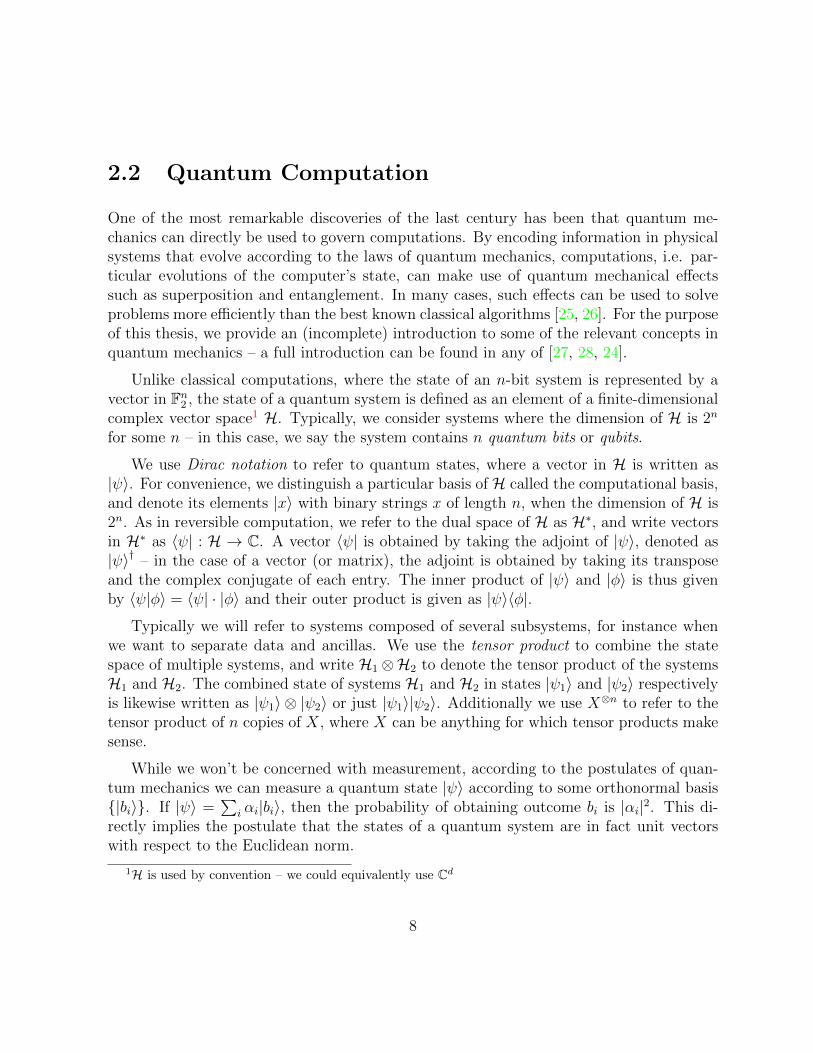
4.2 Visualization of a vp-tree partitioning a set of 2D points. . . . . . . . . . . 36

4.3 Database generation times for minimal depth two qubit circuits. . . . . . . 42

4.4 Database generation and search times for minimal T -depth single qubit cir-cuits. . . . . . . . . . . . . . . . . . . . . . . . . . . . . . . . . . . . . . . . 43

4.5 Controlled Paulis. . . . . . . . . . . . . . . . . . . . . . . . . . . . . . . . . 44

4.6 Logical gate implementations of controlled unitaries without ancillas. . . . 44

4.7 W gate (depth 9). . . . . . . . . . . . . . . . . . . . . . . . . . . . . . . . . 45

4.8 3-qubit logical gates with no ancillas. . . . . . . . . . . . . . . . . . . . . . 46

4.9 Reduced T -depth implementations utilizing ancillas. . . . . . . . . . . . . . 47

4.10 Addition of one ancilla reduces the minimum circuit depth from 7 to 6. . . 47

4.11 Controlled-T gate (depth 19). . . . . . . . . . . . . . . . . . . . . . . . . . 48

4.12 Circuit implementing a reversible 1-bit full adder. . . . . . . . . . . . . . . 48

4.13 Circuit implementing a controlled-H gate (T -depth 1, total depth 9). . . . 49

4.14 Circuit implementing a Toffoli gate (T -depth 3, total depth 9). . . . . . . . 49

x

5.1 Implementation of a Λ3(X) gate [1]. . . . . . . . . . . . . . . . . . . . . . . 53

5.2 Optimized Clifford + T implementation of a Λ3(X) gate. . . . . . . . . . . 53

5.3 {CNOT, T} circuit implementing the doubly controlled Z gate. . . . . . . 56

5.4 A circuit giving a non-optimal (in the T -count) phase expression. . . . . . 57

5.5 T -depth 1 implementation of Figure 5.4 with one ancilla. . . . . . . . . . . 59

5.6 Clifford + T implementation of the Toffoli gate with the target on qubit 3. 65

5.7 Gate update rules. A gate Ui denotes gate U applied to qubit i, CNOT(i,j)

specifies i as the control qubit and j as the target. . . . . . . . . . . . . . . 70

5.8 6-bit Cuccaro adder without expanding Toffoli gates [2]. . . . . . . . . . . 75

5.9 Optimized circuit from Figure 5.8 after expanding Toffolis. T -count wasreduced from 77 to 63 and T -depth was reduced from 33 to 27. . . . . . . . 76

5.10 T -depth 1 implementation of the Toffoli gate. . . . . . . . . . . . . . . . . 77

5.11 T -depth 2 implementation of the Toffoli gate. . . . . . . . . . . . . . . . . 77

5.12 T -depth 3 implementation of the controlled-T gate. . . . . . . . . . . . . . 77

5.13 Λ3(X) gate. . . . . . . . . . . . . . . . . . . . . . . . . . . . . . . . . . . . 78

xi

Chapter 1

Introduction

Circuit optimization, believed to be an intractable problem [3], is an important part of thedesign and construction of classical computational devices. The ability to produce smaller,energy efficient integrated circuits relies heavily on the ability to reduce the logical com-plexity of the circuit’s functionality, especially with the gradual slowing of improvements totransistor technology. Accordingly, researchers have developed effective heuristic methodsfor minimizing logic in integrated circuits, notably the well-known Quine-McCluskey andESPRESSO algorithms [4], the latter of which is used as a standard optimization procedurein modern logic synthesis tools and VLSI design.

Given the initially limited quantum computational resources available, in order to han-dle interesting problem sizes it will be even more important to reduce the resources requiredto implement a given quantum circuit through similar circuit optimization. In fact, as real-istic quantum computers will likely require some fault tolerance scheme where the amountof error correction is proportional to the resources used, the effect of circuit optimizationsbecomes even more profound. While current experimental circuits can be optimized byhand, recent advances in quantum information processing devices (e.g. [5], [6], [7], [8])and improvements to fault-tolerant thresholds (e.g. [9], [10], [11]) hint at the prospect ofscalable quantum devices. As a result, there is a growing need for quantum circuit opti-mization tools that can be applied to large quantum circuits, in order to allow the bestpossible use of these new computational devices.

Unfortunately, few tools have to this point been developed for the direct purpose ofoptimizing quantum circuits. While techniques and recent breakthroughs in reversiblecircuit optimizations [12, 13, 14] are applicable to the classical subset of quantum com-putation, this leaves out a large class of quantum circuits from consideration – moreover,

1

reversible circuits themselves usually require higher level logic (e.g. Toffoli gates) that mustbe decomposed to a fault tolerant quantum gate set. Likewise, while there exist synthesismethods that can be used to optimize circuits, they are limited to single-qubit circuits, orare otherwise impractical for multi-qubit circuits. Recent developments in quantum circuitoptimization [15, 16, 17] show promise, but the landscape still remains fairly barren.

This thesis makes progress on developing algorithms and techniques for optimizingquantum circuits themselves, both for large scale and small scale circuit optimization. Thetwo approaches are complimentary in that small, common operations can be optimizedexactly, while large compound circuits can be further optimized according to less effectivebut more efficient methods. In the first part of this thesis, we develop an algorithmand related techniques for finding exactly optimal circuits in exponential time, leadingto efficient circuits for common quantum operations. In the second part, we build a familyof heuristic polynomial time algorithms for optimization of large quantum circuits.

One pervading theme of this thesis is the optimization of fault-tolerant circuits, circuitscomposed of logical gates on encoded groups of qubits. Given the fragile nature of qubits,the prospects of scalable quantum computing without some systematic way of mitigatingphysical errors and noise are bleak – for this reason, we look to fault tolerance to guide opti-mization. In particular, the notions of T -count and T -depth, motivated by fault tolerance,inform many of our constructions.

1.1 Overview of Thesis

The thesis is organized as follows. Chapters 2 and 3 provide mathematical preliminariesand background. In Chapter 2 we briefly describe reversible and quantum computation,and define the notation and some basic lemmas we will use. Chapter 3 provides a shortsurvey of the current state of quantum circuit optimization.

Chapters 4 and 5 present original work on the optimization of quantum circuits. Chap-ter 4 describes a general algorithm for speeding up brute-force optimization of quantumcircuits, as well as search space reductions to make the algorithm more practical. Thealgorithm is motivated by the need to compile higher level gates into lower level gate setsin a depth-optimal way as circuit depth directly affects the run-time, and by extensionthe error rates. We then use this algorithm to compute depth-optimal decompositions ofmany common quantum gates into the standard fault-tolerant “Clifford + T” gate set. Wealso describe how to modify the algorithm to incorporate other cost metrics, ancillas, andsynthesize approximate circuits.

2

In contrast to the algorithm described in Chapter 4, Chapter 5 presents a polynomial-time quantum circuit optimization algorithm that is shown to scale well to large, practicalquantum circuits. The algorithm re-synthesizes quantum circuits consisting of Clifford+ T gates while minimizing the number of T gates and placing them in parallel. Suchproperties have very recently become common optimization concerns [18, 19, 20, 21], as Tgates require state distillation in the common fault tolerant quantum computing schemes– in fact, Fowler [22] describes how to perform fault tolerant quantum computation in oneround of measurement per stage of parallel T gates. As a byproduct, we also reduce exactminimization of T -count to the minimization of polynomial equations in mixed arithmetic.This algorithm also represents progress towards the automated usage of ancillas in depthoptimizations, as the usage of ancillas comes at effectively no performance cost.

3

Chapter 2

Reversible and QuantumComputation

In this chapter we detail the notions of reversible and quantum computation that will berelevant to the material presented in this thesis. We begin with an account of reversiblecomputation, then extend this to cover quantum computations. As the optimizationswe develop will be designed with fault tolerant circuits in mind, we end off with a briefdiscussion of quantum fault tolerance.

2.1 Reversible Computation

Classical computation is typically performed irreversibly – the inputs to a computationcannot generally be recovered from the outputs, and so the computation cannot be undoneor reversed. It was Landauer who first noticed that this process, in effect destroyinginformation, results in a dissipation of energy in the form of heat or noise [23]. Classicalcomputers built from the irreversible NAND gate – defined as the two-input logic gate thatreturns 0 if and only if both inputs are 1 – thus waste huge quantities of energy throughthe process of constantly discarding information.

We could instead consider a model of classical computation in which computations arereversible. In particular, we will define a circuit model of classical computation that permitsa straightforward restriction to reversible computations, which we see is equally powerful.While we are mostly interested in reversible computations as the classical subset of quantum

4

computations, the promise of low-power electronics has led researchers to seriously considerreversible computing models as an alternative to traditional digital logic.

While we save many details of circuit model for Section 2.3, which defines the moregeneral quantum circuit model, we describe a few basic notions here. In the classical circuitmodel of computation, wires carry bits of information to logic gates, which produce newbits of information. The state of an individual bit can be represented as a binary valueb ∈ F2, where F2 = {0, 1} is the two element finite field with multiplication and additioncorresponding to logical AND (∧) and exclusive-OR (⊕), respectively – the representationof F2 as a field is not strictly necessary, but will help to classify types of classical functions.The state of a system of n bits is then represented by a binary string of length n orequivalently a vector in Fn2 ; likewise, classical functions map n-bit strings to m-bit strings,i.e. classical functions are operators f : Fn2 → Fm2 . We typically refer to classical functionsas just functions, and if m = 1 we call f a Boolean function. An individual logic gateimplements a particular function on its input bits, and a circuit threads bits through asequence of gates.

∧

∧

∨

x1

x2

⊕

⊕

Figure 2.1: An example of a classical circuit computing x1 ⊕ x2.

We define a set G of classical gates as universal for classical computations if and only ifany classical function f can be computed by a circuit using only gates in G. In particular,NAND (along with the ability to copy bits) is universal for classical computation. Whilewe won’t be particularly concerned with universality for classical computation, it will laterplay a more significant role in quantum computation.

In restricting our attention to the reversible circuit model, we require that logic gatesimplement invertible functions – in other words, classical functions f : Fn2 → Fm2 such thatf−1 exists. As a result, the universal gate NAND no longer applies in the reversible model,and moreover no (reversible) gate set alone is universal simply by noting that a classicalfunction f : Fn2 → Fm2 may not be invertible and thus cannot be implemented directly.

We can recover universality by allowing the use of ancillas, bits that can be initializedto either 0 or 1, as a kind of temporary register. Under this assumption, the reversible

5

Toffoli gate,TOF (x1, x2, x3) = (x1, x2, x3 ⊕ (x1 ∧ x2)),

is universal, by noting that TOF (x1, x2, 1) = (x1, x2, NAND(x1, x2)) and TOF (x1, 1, 0) =(x1, 1, x1), i.e. the Toffoli gate can implement both NAND and copy bits. Of course, weneed a way to reclaim the ancillas after a computation is finished, otherwise computationswill continue to grow in space. One option is to erase the partial information containedin the ancillas – while this solution is suitable for classical computations, discarding suchinformation can have a profound effect on the output in a quantum computation. Anotheroption that avoids this problem in the quantum case is to copy the outputs to fresh ancillas,then uncompute f by applying f † = f−1 to free up the used ancillas.

x1

x2

xn...

...

...

f f †

|0〉

Figure 2.2: An example of a circuit reversibly computing f and cleaning up ancillas.

The addition of ancillary bits complicates our mathematical formalism to an extent.While a function f that accepts n primary inputs and N − n ancillary bits (without lossof generality assume they are initialized to the 0 state) can be described as a classicalfunction over FN2 , we only really care about its affect on some dimension n subspace Vof FN2 . Though a seemingly inconsequential point, it will allow more precise analysis ofcomputations using ancillas.

2.1.1 Linear functions

In this thesis, we will be particularly interested in classical functions that are linear overF2; recall that f : Fn2 → Fm2 is linear if f(x ⊕ y) = f(x) ⊕ f(y) for every x, y ∈ Fn2 . Thecontrolled-NOT gate

CNOT (x1, x2) = (x1, x1 ⊕ x2),

is an example of a linear reversible gate. As an important result, the set of all linearreversible functions are those that can be computed by only using CNOT gates [14].

6

Before ending off the discussion of reversible circuits, we turn our attention to classicalfunctions which are both linear and Boolean, and how such functions can be implementedreversibly. As linear Boolean functions are linear transformations Fn2 → F2 and are thusrepresented by 1 × n matrices over F2, we can see them as (column) vectors in the dualvector space Fn∗2 of Fn2 . In this view, any state x in Fn2 is also a linear Boolean functionxT , and vice versa, where xT denotes the matrix transpose of x. This viewpoint has theadvantage that we can view states as either vectors or functions, and apply definitions andtheorems from linear algebra to linear Boolean functions, most notably those related todimension.

Definition 1. Given a set of linear Boolean functions S ⊆ Fn∗2 , the rank of S, denotedrank(S) is the dimension of the subspace spanned by the vectors in S.

As we will primarily be concerned with reversible computations, we prove a lemmarelating linear Boolean functions to linear reversible functions.

Lemma 1. Given a subspace V of FN2 and a set of linear Boolean functionsS = {f1, f2 . . . fN} ⊆ V ∗, the linear surjective function f : V → W defined as

f(a1, a2, . . . , aN) = (f1(a1, . . . , aN), . . . , fN(a1, . . . , aN))

is reversible if and only if rank(S) = dim(V ).

Proof. Reversibility follows if and only if rank(S) = dim(V ) due to a straightforwardapplication of the rank-nullity theorem; dim(im(f)) + dim(ker(f)) = dim(V ). As thefunctions in S form the row vectors of f , rank(S) = dim(im(f)) = dim(W ) and so f isone-to-one if and only if rank(S) = dim(V ). Thus f is invertible on its image W , i.e., thereexists f−1 : W → V such that ff−1 = f−1f = I.

As a consequence of Lemma 1, we establish criteria on when a set S of linear Booleanfunctions can be computed simultaneously over an N -bit state space V – specifically, ifthere is a size N superset S ′ of S with dimension dim(V ), there is a reversible circuitwith outputs computing S ⊆ S ′. We use this criteria to define the notion of (reversible)computability on sets of linear Boolean functions – as we will henceforth be concernedstrictly with reversible computations, we omit the qualifier reversible in further discussions.

Definition 2. Given a dimension n subspace V of FN2 , a set S ⊆ V ∗ is (reversibly)computable over V if there exists a size N superset S ′ of S such that rank(S ′) = n.

7

2.2 Quantum Computation

One of the most remarkable discoveries of the last century has been that quantum me-chanics can directly be used to govern computations. By encoding information in physicalsystems that evolve according to the laws of quantum mechanics, computations, i.e. par-ticular evolutions of the computer’s state, can make use of quantum mechanical effectssuch as superposition and entanglement. In many cases, such effects can be used to solveproblems more efficiently than the best known classical algorithms [25, 26]. For the purposeof this thesis, we provide an (incomplete) introduction to some of the relevant concepts inquantum mechanics – a full introduction can be found in any of [27, 28, 24].

Unlike classical computations, where the state of an n-bit system is represented by avector in Fn2 , the state of a quantum system is defined as an element of a finite-dimensionalcomplex vector space1 H. Typically, we consider systems where the dimension of H is 2n

for some n – in this case, we say the system contains n quantum bits or qubits.

We use Dirac notation to refer to quantum states, where a vector in H is written as|ψ〉. For convenience, we distinguish a particular basis of H called the computational basis,and denote its elements |x〉 with binary strings x of length n, when the dimension of H is2n. As in reversible computation, we refer to the dual space of H as H∗, and write vectorsin H∗ as 〈ψ| : H → C. A vector 〈ψ| is obtained by taking the adjoint of |ψ〉, denoted as|ψ〉† – in the case of a vector (or matrix), the adjoint is obtained by taking its transposeand the complex conjugate of each entry. The inner product of |ψ〉 and |φ〉 is thus givenby 〈ψ|φ〉 = 〈ψ| · |φ〉 and their outer product is given as |ψ〉〈φ|.

Typically we will refer to systems composed of several subsystems, for instance whenwe want to separate data and ancillas. We use the tensor product to combine the statespace of multiple systems, and write H1⊗H2 to denote the tensor product of the systemsH1 and H2. The combined state of systems H1 and H2 in states |ψ1〉 and |ψ2〉 respectivelyis likewise written as |ψ1〉 ⊗ |ψ2〉 or just |ψ1〉|ψ2〉. Additionally we use X⊗n to refer to thetensor product of n copies of X, where X can be anything for which tensor products makesense.

While we won’t be concerned with measurement, according to the postulates of quan-tum mechanics we can measure a quantum state |ψ〉 according to some orthonormal basis{|bi〉}. If |ψ〉 =

∑i αi|bi〉, then the probability of obtaining outcome bi is |αi|2. This di-

rectly implies the postulate that the states of a quantum system are in fact unit vectorswith respect to the Euclidean norm.

1H is used by convention – we could equivalently use Cd

8

Quantum mechanics also postulates that the evolution of a closed system is unitary,meaning quantum states must evolve according to unitary operators U : H → H. Byunitary we mean that U is a linear operator on H such that U †U = UU † = I, i.e. U isinvertible with U−1 = U †. Equivalently, U is a linear operator that preserves the Euclideannorm. We denote U(d) to denote the set of unitary operators on a complex vector spaceof dimension d. For instance, the Hadamard gate

H =1√2

(1 11 −1

)is an example of a unitary operator. We also distinguish the set SU(d) of unitaries withdeterminant 1, i.e. the unitaries that are unique up to multiples of eiθ, as global phasedoes not affect measurement outcomes.

At this point we can view a correspondence between reversible and quantum compu-tations. As the computational basis consists of all n bit strings, the basis states of aquantum system can be seen to be the set of classical states on the same number of bits.We might then consider the relation between reversible functions and unitary operators.In particular, any unitary U ∈ U(2n) that is a permutation operator in the computationalbasis implements some function f : Fn2 → Fn2 ; since U is unitary, we also know that U isinvertible and thus f is a reversible function. Likewise, any classical reversible functionf can be computed on a quantum computer by a permutation U : |x〉 7→ |f(x)〉 wherex ∈ Fn2 , since the (complex conjugate) transpose of a permutation matrix trivially gives itsinverse.

2.3 The Quantum Circuit model

To provide a concrete model for quantum computation, we describe the quantum circuitmodel, one of the most prominent models of quantum computation (see [24] for a moredetailed exposition).

The quantum circuit model is analogous to the classical or reversible circuit models,in that information – in this case, qubits – is carried on wires through gates which trans-form their state. For a system with n wires, the state space H has dimension 2n, withcomputational basis states corresponding to the 2n elements of Fn2 . In accordance with thepostulates of quantum mechanics, quantum gates are unitary operators on subsystems ofH, depending on which qubits the gate is applied to – more accurately, a gate is the tensorproduct of a unitary together with the identity operator (I) on the unaffected qubits. If

9

two adjacent gates are applied to non-overlapping sets of qubits, they can be written as asingle tensor product and are said to be applied in parallel: (g1 ⊗ I)(I ⊗ g2) = g1 ⊗ g2.

A circuit on n qubits is a finite sequence i 7→ Ui of gates applied in order from left toright to subsets of the n qubits, the effect of which is the functional composition Uk · · ·U2U1

of the individual unitary operators corresponding to the gates. We use UC to refer to theunitary computed by a circuit C so that we can refer to distinct circuits that compute thesame unitary. Though we will mostly ignore measurements, a quantum circuit may alsocontain measurement operators over a given basis and wires carrying classical data emittedfrom such measurements.

H P T

• H P

• • H

Figure 2.3: An example of a quantum circuit, implementing the quantum Fourier transformup to permutation of the outputs.

We define the depth of a quantum circuit as the maximum length of a path through thecircuit. By path we mean a path in the directed acyclic graph representing the circuit, withnodes corresponding to the circuit’s gates and edges corresponding to gate inputs/outputs.We will often refer to depths of specific gates in a circuit – e.g. T -depth – in which casewe mean the maximum number of that gate in any path. As an example, the maximumpath length in Figure 2.3 is 5.

A quantum circuit is typically expressed over a particular set of gates. We call a setof quantum gates G a gate set or instruction set, and say that C is a circuit over G if Cis a quantum circuit containing only gates in G; we denote the set of all such circuits 〈G〉.We also define the closure of G over inversion as G† = G ∪ {g†|g ∈ G} and all n-fold tensorproducts of the individual gates2 as Gn. We note that for any G, Gn ⊆ U(2n), and thenotion of circuit depth corresponds to the number of gates in Gn used in the circuit. Infact, we see that the minimum depth of any circuit over G implementing U ∈ U(2n) is theminimum number of gates in Gn needed to implement U .

Lemma 2. A unitary U ∈ U(2n) is implemented by a circuit of depth k over G if and onlyif U = Uk · · ·U2U1 where U1, U2, . . . , Uk ∈ Gn.

2n-fold tensor products of individual gates are commonly called elementary transformations [28]

10

2.3.1 Quantum gates

We now describe some of the common gates and groups of gates that we will use. Forinstance, the Pauli gates,

I =

(1 00 1

)X =

(0 11 0

)Y =

(0 −ii 0

)Z =

(1 00 −1

),

are commonly used to model error channels and are very important in the constructionand analysis of quantum error correcting codes. We use Pn to refer to the set of n-foldtensor products of the Pauli gates.

Another important class of gates include the Hadamard (H), controlled-not (CNOT ),and Phase (P ) gates,

H =1√2

(1 11 −1

)CNOT =

1 0 0 00 1 0 00 0 0 10 0 1 0

P =

(1 00 i

).

The Hadamard, CNOT, and Phase gates generate a group of unitaries called the Cliffordgroup, denoted C. The Clifford group on n qubits is equivalent to the normalizer of thePauli group Pn, Cn = {U ∈ U(2n)|UPnU−1 ⊆ Pn}, and as a consequence contains the Pauligroup as well. Remarkably, Gottesman and Knill [29] proved that any circuit composedof Clifford group gates can be efficiently simulated on a classical computer, and so suchcircuits clearly cannot perform all quantum computations.

We will also commonly refer to the previously seen Toffoli (TOF ) gate, and the π/8gate (T ):

TOF =

1 0 0 0 0 0 0 00 1 0 0 0 0 0 00 0 1 0 0 0 0 00 0 0 1 0 0 0 00 0 0 0 1 0 0 00 0 0 0 0 1 0 00 0 0 0 0 0 0 10 0 0 0 0 0 1 0

T =

(1 00 eiπ/4

).

Both the Toffoli and π/8 gates lie outside of the Clifford group, which make them usefulfor general quantum computing.

11

We note that each of the above gates are expressed as matrices over the ring Z[

1√2, i],

or equivalently the ring of dyadic fractions Z[

12

]extended with ω = eiπ/4. Recent results

have shown that any unitary over Z[

1√2, i]

can in fact be implemented over C∪{T} [30, 31].

The notion of controlled quantum gates will also be important throughout this thesis.We define a controlled-U gate as Λ(U) : |x〉|ψ〉 7→ |x〉Ux|ψ〉, where x ∈ {0, 1}; in a circuit,we typically use a solid dot to represent a control with a line to the controlled gate U . Wecan write a unitary matrix for a controlled-U gate as Λ(U) = |0〉〈0| ⊗ I + |1〉〈1| ⊗ U :

(|0〉〈0| ⊗ I + |1〉〈1| ⊗ U)|x〉|ψ〉 = 〈0|x〉|0〉 ⊗ |ψ〉+ 〈1|x〉|1〉 ⊗ U |ψ〉 = |x〉Ux|ψ〉.

We can further define Λm recursively as Λ (Λm−1(U)), where m gives the number of controlson U . The previously shown gates CNOT and TOF are in fact controlled X gates:

CNOT = Λ(X), TOF = Λ2(X).

One important observation about the nature of controlled operations is that if thereexists a circuit over G implementing Λ(g) for each g ∈ G, then for any unitary U imple-mented by a circuit over G, Λm(U) can also be implemented over G. This is a result of thefollowing lemma:

Lemma 3. Suppose U = Uk · · ·U2U1 for some unitaries U,U1, U2, . . . , Uk ∈ U(2n). Then

Λ(U) = Λ(Uk) · · ·Λ(U2)Λ(U1).

A simple method for constructing such a circuit then proceeds by replacing every gateg with a circuit for Λ(g).

2.3.2 Universal gate sets

As in the classical case, we need to know which gate sets can be used to implement theset of quantum computations, U(2n). An immediate observation is that since there areuncountably many unitaries on any number of qubits, any gate set that can implement allquantum computations is necessarily uncountable in size. It turns out that U(2)∪{CNOT}can implement any quantum computation [1], though constructing such a gate set faulttolerantly would however be extremely unlikely. Instead we consider the possibility ofapproximating some quantum operations.

12

Definition 3. For unitaries U, V ∈ U(2n), U is an ε-approximation of V if ||U − V || ≤ εwhere

||U − V || = max|ψ〉||(U − V )|ψ〉|| =

√〈ψ|(U − V )†(U − V )|ψ〉

is the operator norm.

The operator norm is used as it corresponds closely to the maximum difference in theprobability of obtaining a particular measurement outcome between U |ψ〉 and V |ψ〉. Ingeneral we may want to use different norms to define the error in approximations.

Definition 4. A gate set G is universal for quantum computation if for any unitary U andε > 0, there exists a circuit C over G such that UC is an ε-approximation of U .

As a well-known result, Cn along with any unitary U /∈ Cn is universal [32]. Since{H,P,CNOT} generates the Clifford group up to global phase and P = T 2, the gate setconsisting of {H,CNOT, T} is universal for quantum computing. The set {H,TOF} isalso known to be universal, though it is not as common in fault-tolerant models.

A natural question to ask is how many gates from a universal set are needed to ap-proximate a given unitary U to a desired accuracy – if the approximation is inefficient,any advantage of a quantum algorithm could be negated by the overhead for approxima-tion. Fortunately, it turns out that only an overhead poly-logarithmic in 1/ε is required toapproximate a given unitary, a result known as the Solovay-Kitaev theorem [33].

Theorem 1. (Solovay-Kitaev)

Suppose G is a finite gate set and is universal for single qubit computations. Then forany single qubit unitary U and ε > 0, there is a circuit over G† with length O(logc(1/ε))that is an ε-approximation of U , where c is a positive constant.

2.4 Fault Tolerance

The mathematical models previously described have assumed that computations can beperformed exactly and without error. However, these models are idealized abstractionsof physical and particularly imperfect processes. In any realistic device individual gatesand operations may fail without warning or perform the wrong operation. At this pointwe have two choices: ignore the errors and hope they don’t accumulate too much, or tryto reduce the number of errors by shielding the information from the imperfect physicalprocesses.

13

In the classical world, the first approach is widely used, as the error rates on most mod-ern logic gates are insignificant for most computations of interest. For more fragile classicalprocesses such as communication over noisy channels and data storage, the information iscommonly protected with error correction. Similarly, quantum processes are very error-prone and individual qubits decohere even when they are not being manipulated, so it ishard to imagine large-scale quantum computations without some method for mitigatingthese errors.

A common approach is to use an error-correcting code (ECC) to encode the state of agroup of logical qubits into many physical qubits, then perform logical gates directly on theencoded qubits by encoding the gates in a fault-tolerant manner. For the purposes of thisthesis, we will primarily be concerned with the latter idea, as the construction of encodedgates informs our gate sets and optimization criteria – for this reason, the description willbe cursory.

Error correcting codes, both classical and quantum, encode the state of a logical k-bitsystem in the state of a physical n-bit system by using codewords. The codewords rely onstoring redundant information, so that if one bit fails the remaining bits can be used todetermine the encoded information. In classical error correction, this can be accomplishedby simply repeating the encoded information, though many more efficient codes exist. Asan example, the three bit code encodes a logical 0 state as 000, and the logical 1 stateas 111 – if at most one error occurs on a physical bit, the logical bit can be retrieved bytaking the majority of all three bits.

For quantum error correcting codes, arbitrary quantum states cannot be copied andrepeated to create the encoded state, a consequence of the no-cloning theorem [34]. Instead,quantum error correcting codes assign codewords to the computational basis states of thelogical system. In this way, classical error correcting codes can double as quantum errorcorrecting codes, such as the three bit code which, in a quantum system, protects againstone bit flip error. Indeed, a large class of quantum error correcting codes, called CSS codes,are built by combining classical codes to protect against both bit flip and phase flip errors.

Another common class of quantum error correcting codes, known as stabilizer codes,define the code space as the set of states that remain unchanged under computations insome Abelian group S ⊆ Pn. Given S ⊆ Pn, the code space generated by S is the setT = {|ψ〉 ∈ H |M |ψ〉 = |ψ〉 ∀M ∈ S}, and S is called the stabilizer of T . As an example,the Steane code is a stabilizer code, with the following stabilizer generators:

I ⊗ I ⊗ I ⊗X ⊗X ⊗X ⊗X, I ⊗ I ⊗ I ⊗ Z ⊗ Z ⊗ Z ⊗ Z,I ⊗X ⊗X ⊗ I ⊗ I ⊗X ⊗X, I ⊗ Z ⊗ Z ⊗ I ⊗ I ⊗ Z ⊗ Z,X ⊗ I ⊗X ⊗ I ⊗X ⊗ I ⊗X, Z ⊗ I ⊗ Z ⊗ I ⊗ Z ⊗ I ⊗ Z

.

14

Additionally, the class of stabilizer codes contains all CSS codes.

As the process of encoding and decoding codewords every time a gate is applied woulddefeat the purpose of quantum error correction, logical gates must also be encoded, possiblyby performing some quantum circuit. However, doing so could cause errors by virtue of thefact that an error on one physical qubit may propagate to errors on other physical qubits.Consider, for instance, the CNOT gate: CNOT · (X ⊗ I)|x1〉|x2〉 = |¬x1〉|¬x1 ⊕ x2〉 =(X⊗X) ·CNOT |x1〉|x2〉. The single X error before the CNOT gate becomes two X errorsafter; if the error correcting code in use can only correct one Pauli error at a time, theoriginally correctable error can no longer be corrected after the CNOT gate is applied.While errors are generally detected and corrected after every operation, the possibility ofan error occurring between the last error correction and the application of a gate cannotbe ruled out, and so logical gates must avoid the problem of error propagation.

The simplest way to avoid error propagation is to perform logical gates transversally,which means to apply an encoded U gate, a physical U gate is applied to each qubit in thephysical system (or pairs of equivalent physical qubits in the case of two qubit unitaries).Errors thus cannot propagate within the same encoded qubit when applying logical gates,since no two encoding qubits interact with one another. Unfortunately, for an arbitrarystabilizer code a full universal gate set cannot be built transversally3 [27], and so othertechniques must be used.

Figure 2.4: Transversal CNOT between two qubits encoded in a 5-qubit code.

In the case when a logical U gate cannot be constructed by applying U transversally, atechnique known as gate teleportation [36] is commonly used together with state distillation[37], a technique for distilling a resource state with high fidelity. As gate teleportationrequires measurement, which is typically much slower than physical gates in quantumcomputer implementations, it is already a more costly procedure than transversal gates,

3Codes can be defined that admit a universal transversal gate set [35], but such codes necessarily gobeyond basic stabilizer code theory.

15

both in terms of time and space. When state distillation is added the effect is compounded,as each round of state distillation typically requires concatenation of error correcting codesalong with complicated logical circuits. These so called “ancilla factories” can requirespace-time volume that is orders of magnitude larger than the resources required for atransversal gate.

It turns out that most of the common CSS codes admit a transversal set of generatorsof the Clifford group [38]. While not strictly speaking transversal, the popular surface codealso has an efficient encoded set of Clifford group generators [10]. Together with resultsfrom measurement-based quantum computing showing that any Clifford group circuit canbe parallelized to constant depth [55], in most fault tolerant schemes it follows that Cliffordgroup operations are extremely fast and space efficient. The non-Clifford operation in auniversal gate set, typically the T gate as it admits reasonable state distillation protocols,is then the bottleneck in fault tolerant computations. Reducing the number of non-Cliffordoperations in a circuit would reduce the number of ancilla states that require preparation,at the same time reducing the fidelity required of each resource state. Likewise, placingT -gates in parallel reduces the amount of time spent waiting for gate teleportation, sincemultiple T gates can be teleported at the same time. Indeed, Fowler [22] shows how toperform fault-tolerant computations in time proportional to one round of measurement perlayer of T -gates, and so the T -depth directly affects circuit run-times. For these reasons,we focus on the topic of T -count and depth optimization for much of this thesis.

16

Chapter 3

Quantum Circuit Optimization

In this section we formally introduce the problem of quantum circuit optimization andreview the state of the art of the field.

The natural intuition is that to optimize a circuit we want to find the best circuit,according to some criteria, implementing the same functionality. We can formalize thisidea, as below, but given that the intuition is clear we refrain from referring to quantumcircuit optimization in such an abstruse way throughout the remainder of this thesis.

Definition 5. (Quantum Circuit Optimization)

Given a circuit C ∈ 〈G〉 and cost function c : 〈G〉 → R, find some C ′ ∈ 〈G〉 such thatUC′ = UC and for any other circuit C0 ∈ 〈G〉 with UC0 = UC , c(C ′) ≤ c(C0).

A closely related problem is that of quantum circuit synthesis, which is concerned withconstructing a circuit implementing or approximating a given unitary. Again, we providea formal definition merely for completeness.

Definition 6. (Quantum Circuit Synthesis)

Given a unitary U ∈ U(2n), gate set G and precision ε ≥ 0, find a circuit C ∈ 〈G〉 suchthat ||U − UC || ≤ ε. If ε = 0 then the problem is referred to as exact synthesis.

The reason we are interested is circuit synthesis is that synthesis algorithms can bedesigned in such a way as to produce circuits optimal in some cost. Such algorithms canthen be used to optimize a circuit C by synthesizing an optimal circuit for UC , assumingUC can be computed in reasonable time. Given that most synthesis algorithms work for a

17

few qubits at most, for circuits that can be optimized by such re-synthesis computing UCshould be fast.

Sometimes we want to relax the optimization and synthesis problems. In particular,we can consider situations where we only need to produce a circuit equivalent up to aglobal phase, i.e. we want C ′ such that UC′ = eiθUC for some θ. We can also considersituations where ancillas may be used to optimize a given cost; in this case we require thatC ′ implements UC′ such that for any |ψ〉 ∈ H, |0〉⊗m ⊗ (UC |ψ〉) = UC′(|0〉⊗m|ψ〉). If thenumber of ancillas that are available is unbounded, we denote m =∞.

The most common families of cost functions on quantum circuits involve gate countsand depth-related costs – in the most basic case, both types of costs have clear motivation inreducing the circuit time and complexity (also indirectly affecting error rates). A weightedgate count assigns a weight to each gate in G, with the cost of a circuit equal to thesum of the cost of each gate. In the case where each gate has weight 1, we just call ca gate count. One particular weighted gate count that we will be concerned with, calledthe T -count and defined as c(T ) = 1, c(g) = 0 ∀g 6= T , arises from the consideration offault tolerant gate constructions where T gates are expensive procedures. Circuit depth,defined earlier, is our other main optimization criteria, and we distinguish T -depth (recall:the maximum number of T gates in a path through the circuit) as an important depthquantity for optimization.

Another class of quantum circuit optimization problems arises when information aboutthe physical architecture is included in the circuits. These problems are typically calledplacement problems, though in many cases (e.g. 2D nearest neighbour) they can be de-scribed as circuit optimization problems with additional constraints. In this thesis we donot consider such problems, though we direct the interested reader to some relevant results[40, 17, 41].

3.1 State of the Art

We review some of the previous results in quantum circuit optimization. As many quantumcircuits have large sections that are strictly reversible circuits, for instance the reversiblearithmetic in Shor’s factoring algorithm [25], it is useful to lift reversible circuit optimiza-tions to the quantum domain. Algorithms designed for optimal synthesis are also includedin the discussion, though algorithms not covered here, such as [42], may also relevant froman optimization point of view in some restricted cases.

18

3.1.1 Exhaustive search

A large class of optimal synthesis algorithms work by exhaustively enumerating all circuitsand returning the lowest cost circuit implementing the desired computation; this techniqueis commonly called exhaustive or brute-force searching. This method is particularly popularin the circuit synthesis community as a way of optimally compiling small commonly usedgates or functions to the target gate set, and in these small instances it can be very effective.

Typical exhaustive search algorithms generate circuits in increasing size or depth, com-bined with heuristics to reduce the number of candidates to be generated. Such a searchis called a breadth-first search, as the space of circuits over a gate set G can be viewedas a tree where each branch corresponds to the next gate in the circuit. Breadth-firstsearches are thus naturally tuned to optimize size and depth, though they can be usedindirectly to optimize other costs. Such searches also typically involve the computationof some database of circuits, where the database is computed once and loaded whenever anew circuit is needed. If the database provides efficient lookups, circuits that are alreadyin the database can be synthesized efficiently.

This technique has been used extensively in the optimal synthesis of reversible functions.Shende et al. [43] used a breadth-first search to synthesize all minimal gate count circuits forreversible functions on 3 bits, over the gate set {X,CNOT, TOF}. Their algorithm buildsdatabases of optimal circuits up to a maximum gate count, and they devise a recursivescheme for increasing the search depth where they multiply the target function with someknown permutation and synthesize the resulting function. Maslov and Miller [44] laterexpanded on those techniques and adapted them to synthesize all reversible functions on 3bits over the quantum gate set {X,CNOT,Λ(V ),Λ(V †)}. In particular, they reduced thesearch space by only storing functions the are unique up to relabeling of the inputs andoutputs. Their approach, however, did not allow control qubits to carry quantum values,e.g. values resulting from a Λ(V ) or Λ(V †) gate, and the resulting circuits are thus notprovably optimal. Golubitsky and Maslov [12] further expanded this technique by removinginverse functions from the circuit databases, which along with other improvements allowedthem to synthesize all optimal 4 bit reversible functions over {Λi(X)|0 ≤ i ≤ 3}. Animportant consideration in these algorithms is the exact representation of functions andcircuits; they typically use compact binary representations of the functions which alloweasy searching over databases and low storage requirements [12].

While breadth-first searches are common in reversible circuit synthesis, the lack ofefficient representations of unitaries make such approaches more difficult. Fowler [45]avoided this problem by performing the breadth-first search directly, i.e. without the use ofa precomputed database implementing efficient lookup. His algorithm finds optimal gate

19

count ε-approximations of unitaries by performing a breadth first search and keeping trackof the set of unique gate sequences up to a given depth. New circuits are then comparedagainst the list of unique circuits and the circuit can be removed from consideration ifsome subcircuit is not unique. Furthermore, he shows how to skip to the next potentiallyunique circuit once such a circuit is found. Despite the expensive process of checking eachsubcircuit, the method proved effective for single qubit circuits over C1∪{T, T †}, and untilrecently was the primary method for computing optimal gate count circuits.

More recently, Bocharov and Svore [19] developed a depth-optimal canonical form forsingle qubit circuits over the gate set {H,T}. They show that databases of canonicalcircuits can be built efficiently, compared to the costly procedure of generating each gatesequence and comparing it with the current database. Such databases are also claimedto use less memory than databases storing unitaries. While the resulting databases canbe searched for ε-approximations efficiently, O(εk2k) for databases consisting of canonicalcircuits with T -count at most k, it requires searching for each element of the double cosetC1UC1 where U is the target unitary. Furthermore, the canonical form applies only tosingle-qubit circuits over {H,T}, and thus cannot be used to compute minimal gate countor minimal depth multi-qubit quantum circuits.

3.1.2 Algorithmic synthesis

In some restricted gate sets and cost metrics, optimal circuits can be synthesized directly,rather than exhaustively searching for a circuit. We review some of the known techniqueshere.

In the reversible circuit domain, SAT solvers have been used to produce optimal gatecount circuits. Hung et al. [13] use multiple-valued logic to synthesize reversible functionsover the gate set {X,CNOT,Λ(V ),Λ(V †)} as in [44] – again, control bits are restricted toBoolean values. The multiple-valued logic synthesis is then performed by bounded modelchecking with a SAT solver, a technique where a transition system is encoded in proposi-tional logic, then paths from an input state to an output state are found by solving SATinstances for increasing path lengths. Along similar lines, Große et al. [46] formulate theproblem of reversible logic synthesis over {Λi(X)|i ≥ 0} as a sequence Boolean satisfiabil-ity problems, which are then solved via SAT solvers. As both algorithms require Booleansatisfiability to be solved, their complexity is effectively no better than exhaustive search –furthermore, exhaustive search has been shown to be more efficient in both cases [44, 12],albeit with greater memory usage.

Non-search based synthesis has occasionally been used in quantum computing. In

20

particular, Kliuchnikov et al. [30] describe an algorithm for decomposing an arbitrary

single-qubit unitary over the ring Z[

1√2, i]

into a circuit over {H,T}. Their method

reduces single-qubit unitary synthesis to computing a circuit preparing a particular state,then they can recursively reduce the complexity of the state by applying HT k for someparticular choice of k ∈ {0, 1, 2, 3}. Furthermore, they prove that the number of T and Hgates in the resulting circuit is optimal, effectively solving T -count optimization for singlequbit circuits over {H,T}. Giles and Selinger [31] further extended this result to a synthesis

method for multi-qubit unitaries over Z[

1√2, i], though the construction is non-optimal in

terms of either gate counts or depth.

Other examples of synthesis in quantum computing focus on approximating unitaries

outside of the Z[

1√2, i]

ring. The classic example is the Solovay-Kitaev algorithm [47], a

recursive algorithm that increases the accuracy of each successive approximation Un−1 byapproximating unitaries V , W such that the residue UU †n−1 is equal to the group com-mutator VWV †W † – furthermore, the unitaries V and W must be balanced, in that theyare both within a particular distance from the identity. While not optimal, the algorithmproduces single-qubit circuits of size O(log3.97(1/ε)), which will be useful for comparingto more recent methods. Specifically, Selinger [48] proved a worst-case lower bound of4 log(1/ε) − 9 T gates to implement a single-qubit z-axis rotation over the Clifford groupand T gates, and at the same time developed an algorithm that approximates a single-qubitz-axis rotation using 4 log(1/ε) + 11 T gates. Kliuchnikov et al. [49] describes another ap-proximation algorithm that appears to achieve T -count of 3.21 log(1/ε)− 6.93 on averagefor ε-approximations of z rotations. Both algorithms proceed by constructing a unitary

over Z[

1√2, i]

approximating the target unitary, then decomposing the approximation op-

timally using [30]. However, these methods are limited to single-qubit unitaries, and theirusefulness regarding circuit optimization is thus limited to circuits containing arbitrarysingle-qubit rotations.

3.1.3 Local rewriting

Very few methods exist for optimizing gate count in large quantum circuits, with themajority of the previous results being devoted to local optimization techniques. Suchtechniques can be loosely categorized as peephole optimizations or template-based opti-mization, both of which involve the replacement of subcircuits with smaller (in gate countor depth) equivalent circuits.

The former grew out of compiler terminology where optimizations are performed on

21

just a few lines of code, as if viewed through a “peephole”. In relation to circuit opti-mization, peephole optimization commonly involves selecting subcircuits then synthesizingan optimal circuit computing the same function. Such a technique is useful in reversiblecircuit optimization, where every function on 4 bits can be synthesized quickly [12]. Prasadet al. [50] develop the technique of peephole optimization and apply it to large reversiblecircuits. Their results show on average 25% reduction in circuit size for random circuits,and circuits with up to a thousand gates could be optimized quickly.

Templates, while a theoretically similar technique, use circuit identities (e.g. C = C ′)to transform the circuit, either in a directed way or to replace subcircuits with smallerequivalent circuits. Miller et al [51] introduced templates for the optimization of reversiblecircuits. In their algorithm, they search for a target template within the algorithm bychoosing an initial gate, then use commutation rules to try and construct the remainderof the template; Maslov et al [52] later expanded on the theory of this technique andintroduced a heuristic modification that produced better results by reducing the numberof control bits.

Template optimization has also had success in being applied to general quantum cir-cuits, particularly by Maslov et al. [15] to the {X,CNOT,Λ(V ),Λ(V †)} gate set – theyshow gate count reductions by over 30% on average for circuits with up to 21 qubits. Sedlakand Plesch [53] also used circuit identities to shift gates as far left as possible, then removeany gates that cancel. While their experimental results, having been applied to CNOTand arbitrary single qubit rotations, are superseded by optimal unitary decompositions[42], they provide further indication for the effectiveness of this method.

3.1.4 Parallelization algorithms

The previously described algorithms have mostly focused on reducing gate counts, and ifthey reduced depth, it was mostly a side effect of reducing gate count. However, as inclassical computing when there are many computational resources available it can oftenmake sense to increase complexity in order to parallelize operations to make use of theextra resources. We review a few of the algorithms for the parallelization of quantumcircuits in this way.

Moore and Nilsson [54] first defined the notion of QNC, a class of quantum compu-tations that can be parallelized to poly-logarithmic depth using a polynomial number ofancillas. While they do not provide an actual algorithm for performing parallelization, theyprove the parallalizeability of a number of gate sets, including {CNOT}, {H} ∪ Λ(P),and encoding/decoding circuits for stabilizer codes. They also provide a large number

22

of transformation rules that could be used to define a parallelization algorithm. Othersimilar results have shown that Clifford group [55] and diagonal unitaries [56] can be par-allelized to constant depth using measurements, though we will primarily be concernedwith measurement-free circuits.

More recently, transformations to and from the measurement-based quantum comput-ing model have been used to parallelize quantum circuits. Broadbent and Kashefi [39]develop an algorithm for the translation of quantum circuits to a pattern (a computationin the measurement-based model) which adds a number of additional ancillas linear in thenumber of gates. The resulting pattern is then optimized by applying rewriting rules ofthe measurement calculus (known as standardization and signal shifting), then the finalpattern is transformed back into a circuit. However, the construction requires that the cir-

cuits are written over the gate set

{Λ(Z), J(α) = 1√

2

(1 e1α

1 e−iα

)}which does not appear to

have fault-tolerant implementations in the common schemes, and requires the availabilityof ancillas. Dias da Silva et al. [16] later expanded this algorithm with new optimizations,and a set of rewrite rules for removing the qubits added during the transformation.

23

Chapter 4

Meet-in-the-Middle: a search-basedsynthesis algorithm

In this chapter we are primarily concerned with the problem of synthesizing a depth-optimalquantum circuit over an arbitrary gate set and with arbitrarily many qubits. The materialpresented here is largely based on [18].

Quantum algorithms are typically described at a high level of abstraction and featuremany common high-level operations, such as the Toffoli gate or integer multiplication.On the other hand, fault-tolerant quantum computation requires specifying circuits interms of a few encoded operations – the high-level operations then have to be compileddown to those low-level encoded gates. In the case of common operations like complexgates, circuits optimizing some particular cost, for instance depth, can be precomputedand substituted in during the compilation process. In particular, circuit depth determinesboth run-time and by extension error rates, hence circuit depth should be the primaryoptimization criteria. However, as evidenced in Chapter 3, algorithms performing this kindof synthesis are lacking in quantum computing; while many methods exist for reversiblecomputation, depth-optimal synthesis of quantum circuits has only been performed onsingle-qubit circuits [45, 19, 30].

To fill this gap, we have developed a practical algorithm for computing depth-optimalfault tolerant circuits. In particular, we describe an algorithm and heuristics for speedingup the brute-force search for minimal depth quantum circuits, given a target unitary.Exhaustive search can in many circumstances be a viable optimization method, particularlywhen more efficient methods are either non-existent or fail to produce quality results. Whencombined with heuristics for reducing the size of the search space, the brute force search

24

can be an effective tool for solving such problems, especially in small instances when thebest possible result is needed. Such techniques have been used very effectively for reversiblecircuit synthesis [43, 44, 12], and have shown better run-times than algorithmic synthesis.

The algorithm, called the meet-in-the-middle algorithm, reduces the time and spacecomplexity of the brute-force search by roughly a square root. In allowing minimal depthcircuits to be computed using only circuits of at most half the minimal depth, the algorithmgenerates just a square root of the circuits that would be generated in a naıve exhaustivesearch. Compared to less naıve approaches, our algorithm provides a space-time trade-offwhich mitigates the major bottleneck of space consumption in such approaches. Addition-ally, we show that the meet-in-the-middle algorithm, while designed with depth-optimalsynthesis in mind, is very flexible and can be used to efficiently optimize different criteriaas well. To further improve the performance, we also detail search space reductions thatdrastically reduce the number of generated circuits.

The methods developed here were largely designed for exact synthesis of quantum cir-cuits – recall that exact synthesis produces circuits that implement the target unitary withno error. As a result, the algorithm is particularly suited for re-synthesis, since an ini-tial decomposition ensures there exists an optimal circuit implementing the same unitaryover the same basis, and individual subcircuits can be re-synthesized without affecting theoverall accuracy of a circuit. The algorithm can, however, can be modified to synthesizecircuits approximating a target unitary; we later develop such a modification and use itto achieve faster depth-optimal circuit approximations than previously known multi-qubitalgorithms.

4.1 The Meet-in-the-middle algorithm

In this section we give a high level description of the meet-in-the-middle algorithm forcomputing depth-optimal quantum circuits over a gate set G. The algorithm is motivatedby the observation that any circuit of minimal depth can be divided into two circuits (orin general, any number of sub-circuits), each of which is a minimal depth circuit – thisidea has been used before in reversible circuit synthesis [43, 12]. As a result, a circuitwith minimal depth l can be found by finding its two halves of depth at most dl/2e. Weshow below that this problem reduces to finding elements in the intersection of two sets ofunitaries.

Lemma 4. Let Si ⊆ U(2n) be the set of all unitaries implementable in depth i over thegate set G. Given a unitary U , there exists a circuit over G of depth l implementing U ifand only if S†bl/2cU ∩ Sdl/2e 6= ∅ where S†i = {U †|U ∈ Si}.

25

Proof. Suppose some depth l circuit C implements U . We divide C into two circuits ofdepth bl/2c and dl/2e, implementing unitaries V ∈ Sbl/2c andW ∈ Sdl/2e respectively, where

VW = U . Since we know W = V †U ∈ S†bl/2cU , we can observe that W ∈ S†bl/2cU ∩ Sdl/2e,as required.

Suppose instead S†bl/2cU ∩Sdl/2e 6= ∅. We see that there exists some W ∈ S†bl/2cU ∩Sdl/2e,and moreover by definition W = V †U for some V † ∈ S†bl/2c. Since W ∈ Sdl/2e, VW = U is

implementable by some circuit of depth bl/2c+dl/2e = l/2, thus completing the proof.

V

W

U

U

U

U

U

†

S Ui†

jS

Figure 4.1: For each V ∈ Si we construct W = V †U and search for W in Sj.

Using this lemma, we can describe a simple algorithm that determines whether thereexists a circuit over G of depth at most l implementing unitary U , and if so return aminimum depth circuit implementing U . Given an instruction set G and unitary U , werepeatedly generate circuits of increasing depth, then use them to search for circuits im-plementing U with up to twice the depth. Specifically, at each step we generate all depthi circuits Si by extending the depth i − 1 circuits with one more level of depth, then wecompute the sets S†i−1U and S†iU and see if there are any collisions with Si (Figure 4.1).By Lemma 4, there exists a circuit of depth 2i − 1 or 2i implementing U if and only ifS†i−1U ∩ Si 6= ∅ or S†iU ∩ Si 6= ∅, respectively, so the algorithm terminates at the smallestdepth less than or equal to l for which there exists a circuit implementing U . In the casewhere U can be implemented in depth at most l, the algorithm returns one such circuit ofminimal depth. The algorithm is given as pseudo-code in Algorithm 1.

As this algorithm requires the computation of S†iU , it relies on the ability to quicklymultiply unitaries. While this is not practical for large numbers of qubits, for the small

26

Algorithm 1 Meet-in-the-middle algorithm.

function MITM(G, U , l)S0 := {I}i := 1for i ≤ dl/2e do

Si := GnSi−1

if S†i−1U ∩ Si 6= ∅ thenreturn any circuit VW s.t.

V ∈ Si−1,W ∈ Si, V †U = Welse if S†iU ∩ Si 6= ∅ then

return any circuit VW s.t.V,W ∈ Si, V †U = W

end ifi := i+ 1

end forend function

numbers of qubits we’re interested in matrix multiplication is sufficiently fast.

Furthermore, for this algorithm to be advantageous, we need a way of efficiently find-ing S†iU ∩ Sj. Fortunately, we can efficiently find the intersection by imposing a strictlexicographic ordering on unitaries – as a simple example two unitary matrices can beordered according to the first element at which they differ. The set Si can then be sortedwith respect to this ordering in O (|Si| log(|Si|)) time, so that searching for an element ofS†i−1U or S†iU takes time O (log(|Si|)) – in practice, we would maintain Si in a sorted datastructure, rather than sort it at search time.

To achieve a (time) complexity bound we can note that |Si| ≤ |Gn|i, so that the ith

iteration thus takes time bounded above by 3|Gn|i log(|Gn|i). Since∑dl/2e

i=1 |Gn|i log(|Gn|i) ≤∑dl/2ei=1 |Gn|i log(|Gn|dl/2e) and

∑dl/2ei=1 |Gn|i ≤ |Gn|dl/2e

(1 + 1

|Gn|dl/2e−1

), we thus see that the

algorithm runs in O(|Gn|dl/2e log(|Gn|dl/2e)

)time. It can also be noted that |Gn| ∈ O(|G|n),

so the run-time is in O(|G|dn·l/2e log(|G|dn·l/2e)

), rather than O(|G|n·l) as in the case of naıve

searching.

We can achieve better on average by using a hash table instead. By hashing the entriesof the circuit databases a given unitary can be found in time O(1) on average, leading toan average time complexity of O

(|Si|)

to test the emptiness of S†iU ∩ Sj.

27

4.2 Search space reduction

To make the meet-in-the-middle algorithm practical for reasonable sized circuits, effortmust be made to reduce the size of the search space. In this section we describe somereductions to the search space and how they can be combined with the meet-in-the-middlealgorithm; the technique we use may be called “pruning” the search tree, as our goal is toremove redundant circuits from the databases Si, in effect removing further branches frombeing explored.

We begin by noting that if a given unitary U has an implementation over G with depth i,then any simultaneous permutation of its input and output qubits can also be implementedin depth i simply by changing which qubits each individual gate acts on. Likewise, if Gis closed under inversion, i.e. G = G†, then U † also admits a depth i implementation,as if U = Ui · · ·U2U1 with U1, U2, . . . , Ui ∈ Gn, then U †1 , U

†2 , . . . , U

†i ∈ Gn and so U † =

(Ui · · ·U2U1)† = U †1U†2 . . . U

†i is a depth i implementation. These two observations imply

that, given a gate set closed under inversion, we can restrict our attention to unitaries thatare unique up to input/output relabeling and inversion. As we don’t care about globalphase in most cases, we can additionally restrict circuit databases to unitaries that areunique up to global phase factors.

More formally, we define an equivalence relation ∼ on unitaries where U ∼ V if andonly if U is equal to V up to relabeling of the qubits, inversion, or global phase factors.This equivalence relation defines the equivalence class of a unitary U ∈ U(2n), denoted[U ], as {V ∈ U(2n)|U ∼ V } – given a gate set closed under inversion, each unitary in agiven equivalence class has the same minimal circuit depth, up to global phase. We thenfocus only on equivalence class representatives, rather than unitaries themselves, and inparticular only store a circuit for each representative in a given set Si. To do so, we definea canonical representative for each unitary equivalence class, then when a new circuit isgenerated we find the unitary representative and determine whether a circuit implementingit is already known.

We can define a canonical representative for each unitary equivalence class by lexi-cographically ordering unitaries and choosing the smallest unitary as the representative.Since relabeling of the qubits corresponds to simultaneous row and column permutationsof the unitary matrix and the inverse of a unitary is given by its conjugate transpose, givenan n qubit unitary U , all 2n! permutations and inversions of U can be generated and theminimum can be found in O(n!) time. For the small instances of n that the meet-in-the-middle algorithm is designed for, the O(n!) overhead to compute a canonical unitary issmall, while the reducing the search space by a factor of 2n! reduces both space and timeusage significantly.

28

Choosing a canonical unitary up to global phase is more difficult in general. In the case

when the gate set contains only unitaries written over the ring Z[

1√2, i], we can generate

each possible global phase factor in the equivalence class. In particular, eiθ ∈ Z[

1√2, i]

if

and only if θ = kπ4, k ∈ Z [30], so there are only 8 possible global phase factors for any

unitary over Z[

1√2, i]. To find a representative, all 8 · 2n! elements of [U ] are generated,

and only the lexicographically earliest element is kept.

In practice, computing each phase factor causes a significant performance hit, so wesought a more efficient way of removing phase equivalences. We instead pick a referenceelement for each unitary and use it to define the canonical phase of the unitary – byconvention we choose the first (scanning row by row) non-zero element of a unitary matrix.We immediately see that if V = eiφU for unitaries V, U , then the reference elementsof V and U must be related by eiφ. For the reference element reiθ of U , we can thendefine the canonical unitary as e−iθU , so that the reference of V will be rei(θ+φ), and thuse−i(θ+φ)V = e−iθU . Conversely, if e−iφV = e−iθU , then V = ei(φ−θ)U and so V is equivalentto U up to phase.

As a matter of unitary representation, if θ 6= kπ4, k ∈ Z, this phase multiple will take

U outside of the ring Z[

1√2, i]. As a result, we actually remove the constraint that the

canonical unitary is normalized instead; rather than taking e−iθU as the canonical unitary,

we use re−iθU since re−iθ ∈ Z[

1√2, i]. Again we can verify that two unitaries have the same

canonical form if and only if they are equal up to phase: if V = eiφU then re−i(φ+θ)V =re−iθU , and if r1e

−iφV = r2e−iθU then

r1 = |r1e−iφ| · ||V || = ||r1e

−iφV || = ||r2e−iθU || = |r2e

−iθ| · ||U || = r2,

so V = ei(φ−θ)U . While this is a minor detail, it allows comparisons to be performed sym-bolically over the ring, avoiding the need for costly, inaccurate floating point computations.

When generating a given Si, for each circuit C in GnSi−1 we compute the canonical rep-resentative of [UC ], then the database of circuits is searched to determine if another circuitimplementing the representative has already been found. Using suitable data structures,each previous set Sj, 1 ≤ j ≤ i can be searched in O

(log(|Sj|)

)time. If no such circuit is

found, we store a circuit implementing the representative of [U ].

As a subtle point, if only representatives of equivalence classes in depth i and j areused for searching, not every equivalence class in depth i + j will be found. Considersome unitary U = VW where V is a circuit of depth i, and W is a circuit of depth j.

29

If V ′ is the representative of [V ] and W ′ is the representative of [W ], then in general(V ′)†VW /∈ [W ], so just using class representatives to search will not suffice. However,V † ∈ [V ′], so W ∈ [V ′]VW , and thus [V ′]U = [W ′]. Practically speaking, this meansthat any unitary U = VW is found by computing the canonical representatives of [[V ]U ],and so we can search all circuits in minimum depth by storing only equivalence classrepresentatives.

In some cases an exact implementation with the same global phase is required, par-ticularly when the circuit may be controlled on another qubit. While we could computecanonical representatives with respect to qubit relabeling and inversion only, any canonicalphase implementation over G = {H,CNOT, T, T †} can be used to construct the correctglobal phase, if it is implementable over G. It suffices to observe (as follows from [30])that if U is implementable by a circuit over G and a circuit C over G implements eiθU ,then θ = kπ

4for some k ∈ Z. Since (HT †T †)3 = e−i

π4 I, eiθ(HT †T †)3kU = U , so a circuit

implementing U exactly can be generated from C with an additive constant cost.

4.3 Extensions

While useful on its own for computing depth-optimal circuits, the meet-in-the-middle al-gorithm is also very flexible and can be extended in a number of ways. We describe a fewsuch extensions in this section.

4.3.1 Alternative costs

While the meet-in-the-middle algorithm is most naturally suited to optimizing depth, itcan also be used to find minimal circuits in other cost metrics. In particular, any cost thatis strictly increasing, i.e. c(C) < c(C ′) for any strict subcircuit C of a circuit C ′, can beoptimized by the meet-in-the-middle algorithm. Since the cost is strictly increasing, givena solution of cost c, all circuits with cost up to c can be generated and searched using themeet-in-the-middle technique, finding a better circuit if one exists. In particular, searchingfollows Algorithm 1 with the addition of a minimum circuit cost for each database Si,cmin = minU∈Si c(U). Once a circuit C implementing U is found, if c(C) < (cmin(Si))

2, Cmust be a minimal cost circuit.

This method on its own is not particularly useful, as depending on the growth of theminimum circuit cost the depth required to find or verify a minimal cost circuit may beintractable to search, e.g. a cost function that assigns one gate a significantly higher cost

30

than the rest. Instead, the search tree should be pruned by removing from the databasesall circuits with cost greater than that of the candidate solution – this method couldpotentially be very effective if an initial candidate solution is already known, as in caseswhen it is used as a re-synthesis optimization.

In other more specific cases, we can develop specially tuned modifications. Recall thatnon-Clifford group gates are typically much more costly in the common fault tolerantschemes. Given that the Clifford group is finite on any number of qubits, we can directlyoptimize the usage of non-Clifford group gates by modifying the initial gate set. Thegeneral procedure follows by generating the entire Clifford group using a set of generators,then the gate set can be defined as any single non-Clifford gate or any tensor productof non-Clifford group gates conjugated by the Clifford group, depending on whether thenumber of such gates is being optimized or the depth, respectively.

As a specific instance, we demonstrate the optimization of T -depth over the gate set{H,P, P †, CNOT, T, T †}. The algorithm first generates the Clifford group Cn by generatingall minimal depth circuits over G = {H,P, P †, CNOT}. To perform the meet-in-the-middlesearch, we denote T = {T, T †} and set S0 = Cn, then define Si = Cn (Tn \ {I})Si−1. EachSi thus contains every circuit with T -depth i in analogy to the depth-optimal meet-in-the-middle algorithm. Searching then proceeds by computing the intersections S†i−1U ∩ Sito search for T -depth 2i − 1 circuits, and S†iU ∩ Si for T -depth 2i. The full algorithm issummed up in pseudocode below.

Algorithm 2 Meet-in-the-middle algorithm for T -depth.

function MITM-T (G, U , l)S0 := {I}i := 1while Si−1 6= ∅ do

Si := GnSi−1 \ ∪j<iSjend whileCn = ∪j<iSjreturn MITM(Cn(Tn \ {I}), U , l)

end function

Searching in this way becomes challenging for high dimensional state spaces, as the sizeof the Clifford group grows exponentially in the number of qubits. As an illustration, for3 qubits the Clifford group has 92,897,280 elements up to global phase [57], which makessearching using modern computers impractical for more than a couple levels of depth; C4

would not even fit in a computer with a reasonable amount of memory using this method.

31

4.3.2 Ancillas

It is often necessary to add ancillas in order to optimally synthesize a given gate – forinstance, the Λ(T ) gate cannot be synthesized over Clifford group and T gates withoutusing ancillas [30]. The addition of ancillas may also allow lower depth circuits or evenlower gate count circuits to be synthesized, allowing a possible tradeoff between space andtime in quantum computations. As a result, it is important to build optimization toolsthat can make use of ancillary qubits. We develop such a method as an extension to themeet-in-the-middle algorithm – for our purposes, we require that the ancillas are initializedin the |0〉 state and returned to |0〉, though it may be possible to consider arbitrary ancillastates as in [1].

Suppose we have U ∈ U(2n) and we want to synthesize some U ′ ∈ U(2N) so thatU ′(|0〉⊗N−n|ψ〉) = |0〉⊗N−n(U |ψ〉). We could naıvely search for I ⊗ U using the meet-in-the-middle algorithm; however, this over-constrains the problem as U ′ need not act as theidentity operator on any other ancilla state. Furthermore, searching for circuits with Nqubits is exponentially harder than search for circuits with n qubits, while the problem ofsearching for circuits with n qubits and N − n ancillas seems comparable.

To address these issues, we note that any unitary U ′ that maps the input |0〉⊗N−n|ψ〉to |0〉⊗N−n(U |ψ〉) will agree with U on the first 2n rows and columns. We could thenexhaustively search for U in the circuits with unique top left 2n× 2n submatrices to find acircuit implementing U using ancillas. However, in the case of meet-in-the-middle, manycollisions would be lost, as it may be the case that V ′W ′(|0〉⊗N−n|ψ〉) = |0〉⊗N−n(U |ψ〉)but V ′(|0〉⊗N−n|ψ〉) 6= |0〉⊗N−n(V |ψ〉), and likewise for W . In other words, the first 2n rowsand columns of V ′ and W ′ is in general not be enough to specify the action of V ′W ′ on|0〉⊗N−n|ψ〉.

Instead, we note that since |0〉⊗N−n(U |ψ〉) = (I ⊗U)|0〉⊗N−n|ψ〉, we want to find V,Wsuch that VW (|0〉⊗N−n|ψ〉) = (I ⊗ U)|0〉⊗N−n|ψ〉. Then, clearly V †(I ⊗ U)|0〉⊗N−n|ψ〉 =W (|0〉⊗N−n|ψ〉), so we can restrict the sets S†{i−1,i}(I ⊗U) and Si to their action on inputs

of the form |0〉⊗N−n|ψ〉 and determine whether their intersection is non-zero. Practicallyspeaking, this involves comparing the first 2n columns of each possible collision, as V †(I⊗U)may not return the ancillas to the zero state.

One disadvantage of this algorithm is that qubit permutations can no longer be removedfrom the search space, since the entire unitary is require to construct each permutation. Asa result, more circuits need to be generated and searched when using ancillas, though ourexperimental results show that it is still easier to search for N qubit circuits with ancillasthan it is to search for circuits on the same number of qubits and no ancillas.

32

4.3.3 Approximate synthesis

As many interesting unitaries cannot be synthesized exactly, we would like to have methodsfor finding the best circuit approximating a given unitary. Typically, this circuit will onlyneed to approximate the desired unitary to accuracy ε in order to achieve the desired errorbound for the total computation. To deal with such situations, we develop an approximatecircuit synthesis algorithm using the meet-in-the-middle algorithm. Unlike the previousextensions, approximate synthesis is reasonably more involved.

Recall that the approximate synthesis problem involves synthesizing some circuit Cover G so that ||U − UC || ≤ ε for some ε > 0. While we originally defined approximationsusing the operator norm, it will be useful to allow other norms to be used where morespecific distance measures are required (e.g. the diamond norm), or where they are easierto compute (e.g. the Frobenius norm). The techniques we develop apply to all distancemeasures defined by the Schatten p-norms,

||U ||p =(

Tr((U †U

)p/2))1/p

,

the key properties being the unitary invariance of Schatten norms, and that they, like allnorms, obey the triangle inequality. We define a distance measure between two unitaries,d(U, V ), as the norm of their difference, ||U − V ||p for some p – such a distance measureis called a metric. The operator norm, as defined earlier, is equal to the Schatten norm inthe limit as p→∞.

The exact synthesis algorithm relied on Lemma 4 to ensure that a minimal depth circuitimplementing U could be found by looking only at minimal depth circuit halves. To usethe same idea in the approximate synthesis setting, we first derive a similar result.

Lemma 5. Let Si ⊆ U(2n) be the set of all unitaries implementable in depth i over the gateset G. Given a unitary U and ε ≥ 0, there exists a circuit over G of depth l implementingsome U ′ with d(U,U ′) ≤ ε if and only if d(V †U,W ) ≤ ε for some V ∈ Sbl/2c,W ∈ Sdl/2e.

Proof. The lemma is a simple consequence of the unitary invariance of the Schatten p-norms, along with Lemma 4. In particular,

||U − VW ||p = ||V †U − V †VW ||p = ||V †U −W ||p.

33

Lemma 5 implies a meet-in-the-middle algorithm for approximate synthesis, exceptthat instead of finding the intersection between S†bl/2cU and Sdl/se, we need to check for

elements in the approximate intersection {(A,B)|A ∈ S†bl/2cU,B ∈ Sdl/2e, d(A,B) ≤ ε}.Fortunately, this is an instance of the well studied Nearest Neighbour problem, which itselfhas applications to many other fields, e.g. image recognition, DNA sequencing and datacompression.

In particular, given a set S with distance measure d : S×S → R, a nearest neighbour ofa query point q ∈ S in database SD ⊆ S is an element p ∈ SD such that ∀r ∈ SD, d(q, p) ≤d(q, r). We denote the problem of finding such a point NN(q, SD). While it will not affectthe solution in a substantial way, the problem we need to solve is a relaxation to whatwe call the bounded near neighbour problem, denoted NN |ε(q, SD): given q, SD and ε > 0,determine whether there exists p ∈ SD such that d(q, p) ≤ ε.

Given a procedure for computing NN |ε(q, SD) together with Lemma 5 we can mod-ify the meet-in-the-middle algorithm to return approximating circuits, as shown in Algo-rithm 3. Using the analysis of Algorithm 1, the algorithm requires O

(|G|dn·l/2e

)calls to

the bounded near neighbour procedure.

Algorithm 3 Meet-in-the-middle algorithm

function MITM-approx(G, U , l, ε)

S0 := {I}i := 1for i ≤ dl/2e do

Si := GnSi−1

if NN |ε(V †U, Si−1) = W for any V ∈ Si thenreturn VW

else if NN |ε(V †U, Si) = W for any V ∈ Si thenreturn VW

end ifi := i+ 1

end forend function

34

Computing NN |ε(q, SD)

As noted above, the nearest neighbour problem is well studied due to its wide range ofapplications. The techniques can be (roughly) divided into those effective in low dimensionspaces, and those effective in high dimension spaces [58]. In the former case projection-based techniques, which divide and search the space by projecting points onto each di-mension (e.g. k-d trees and R-trees), can be very effective – in fact, the k-d tree has beenpreviously used to implement the ε-net in implementations of the Solovay-Kitaev algorithm[47]. However, these methods scale poorly to situations where the dimension is high, suchas multi-qubit approximate synthesis where unitaries on n qubits have dimension 22n.

For high dimensional data, fewer generic, efficient techniques exist. In some instances,transformations to reduce the high dimensional data to a lower dimension space are avail-able (e.g. the discrete Fourier transform), however they are highly specialized for particularapplications and typically don’t provide exact solutions, as is the case for many commonlocality sensitive hash functions. However, a class of generic data structures has beendeveloped for nearest neighbour searches in metric spaces, namely distance-based indexstructures, or in the case of distance-based trees, metric trees. The common metric treeshave been shown to be very effective for nearest neighbour searching [58], and as a resultwe take this approach.

To efficiently compute NN |ε(q, SD) we use a vantage-point (vp) tree, introduced in [59],which has been shown to be very effective in high dimension similarity search, notablyimage recognition [60]. In analogy to simple binary search trees, which were used to storeand search through circuit databases for exact synthesis, a vantage point tree recursivelysplits the database into two subtrees according to each point’s distance to a distinguishedvantage point. Each node in the tree has a unique vantage point p, with points withindistance µ of p placed in one subtree, while those with distance greater than µ are placedin the other subtree. The radius µ of the partitioning ball can be chosen as the mediandistance between p and each point in the tree; if there are not too many points exactlydistance µ from p, we can see that each subtree contains approximately half the points inthe tree.

The advantage for near-neighbour searching can be seen by observing that for a givensubtree SD with vantage point p and radius µ, if our query point q satisfies d(p, q) ≤ µ− ε,then for any r where d(p, r) > µ,

d(q, r) ≥ |d(p, r)− d(p, q)| > |µ− (µ− ε)| = ε

by the triangle inequality, and thus we only need to search for near neighbours in thesubtree containing those elements less than distance µ from p. A similar identity holds if

35

Figure 4.2: Visualization of a vp-tree partitioning a set of 2D points.

d(p, q) ≥ µ + ε. The obvious drawback is that if µ − ε < d(p, q) ≤ µ + ε, the search mustrecurse on both subtrees. The use of the triangle inequality to, in most cases, remove alarge set of points from consideration forms the basis for many metric trees [58].

Algorithm 4 shows how to build a vp-tree on S in O (n log(n)) time, given a distanceoracle. A detailed analysis of the expected search time can be found in [59] – under specificassumptions regarding the probability distribution of the points, they show that searchingcan be performed in expected time O (log(n)). Our experiments show comparable resultsin the case of unitary searching.

Remarks

In this section we close off the discussion with a few remarks regarding the choice of norms,and the combination of approximate meet-in-the-middle with the search space reductions.

One of the main bottlenecks in approximate meet-in-the-middle comes from having todeal with distance computations, requiring the computationally expensive process of com-puting Schatten norms. In the worst case the bounded near neighbour search becomes a

36

Algorithm 4 vp-tree construction and searching [59]

function vptree(S)if S = ∅ then

return empty treeend ifT.p := p for some p ∈ ST.µ := medianr∈Sd(p, r)T.L := VPTREE({r ∈ S|d(p, r) ≤ T.µ})T.R := VPTREE({r ∈ S|d(p, r) > T.µ})return T

end function

function NN |ε(q, T )x := d(T.p, q)if x ≤ ε then

return T.pelse if x ≤ µ+ ε then

if NN |ε(q, T.L) = p thenreturn p

end ifelse if x > µ− ε then

if NN |ε(q, T.R) = p thenreturn p

end ifend ifreturn “not found”

end function

linear search, requiring the distance between every pair of elements in S†iU ×Sj to be com-puted. Even in the average case, there will still be O(|Si| log(|Sj|)) distance computations

to find elements in the approximate intersection of S†iU and Sj. We thus aim to computenorms as efficiently as possible. Fortunately, in the case of the Frobenius norm (p = 2),we obtain a convenient formula that requires only one matrix multiplication, rather thancomputation of the singular values:

Lemma 6. For U, V ∈ U(2n), ||U − V ||2 =√

2 · 22n − 2 · Re(Tr(U †V ))

Proof. We see that

||U − V ||2 =√

Tr ((U † − V †)(U − V ))

=√

Tr (2I − U †V − (U †V )†)

=

√2 · 22n − Tr(U †V )− (Tr(U †V ))†

=√

2 · 22n − 2 · Re(Tr(U †V )).

37

Approximate meet-in-the-middle also affects the search space reductions used in a non-trivial way. While circuit databases containing only circuit representatives can still begenerated, our method of choosing representatives is no longer sufficient for searching; itmay be the case that ||U − V ||p ≤ ε but ||U ′ − V ′||p > ε for representatives U ′, V ′ of[U ], [V ] respectively. To adapt the search space reductions to cover approximate synthesis,we must instead generate and search for every element in [[V ]U ], rather than just itscanonical representative as in the case of exact synthesis.

However, an issue remains with this approach when using the standard Clifford + T

gate set: since U does not necessarily take its elements from the ring Z[

1√2, i], it may be

an arbitrary phase away from any element in our database. We clearly cannot search forevery possible phase multiple in [[V ]U ], so to find approximations up to a global phase weneed to use a norm invariant under global phase. A reasonable choice would be to defined(U, V ) as ||U ⊗ U † − V ⊗ V †||p for some p. Clearly, d(eiθU, eiφV ) = d(U, V ) for any θ, φ:

||eiθU⊗(eiθU)†−eiφV ⊗(eiφV )†||p = ||eiθe−iθU⊗U †−eiφe−iφV ⊗V †||p = ||U⊗U †−V ⊗V †||p.

The naıve method of computing this norm would require generating and computing thesingular values of a 22n× 22n matrix, which is a significant disadvantage performance wise.However, in the case of the Frobenius norm we see that the phase invariant distance canbe computed at no extra cost.

Lemma 7. For U, V ∈ U(2n), ||U ⊗ U † − V ⊗ V †||2 =√

2 · 24n − 2 · |Tr(U †V )|2

Proof. From Lemma 6 we have ||U⊗U †−V⊗V †||2 =√

2 · 24n − 2 · Re (Tr ((U †V )⊗ (UV †))).Since Tr

((U †V )⊗ (UV †)

)= Tr(U †V ) Tr(V †U) by basic properties of the trace, we see that

2 · Re(Tr((U †V )⊗ (UV †)

))= 2 ·

∣∣Tr(U †V )∣∣2 , completing the proof.

The phase-invariant Frobenius norm was previously used in [45] to synthesize approxi-mate circuits. In both cases, we can see that the Frobenius norm gives an overestimate ofthe approximation error as given by the operator norm, since ||U ||p ≥ ||U ||q for any p ≤ q,and thus can be used to bound the approximation error in the operator norm.

4.4 Implementation details

The meet-in-the-middle algorithm, along with its extensions and search space reductions,were programmed in the C++ programming language; the implementation is available

38

online at http://code.google.com/p/mitms. In this section we discuss some of the relevantimplementation details for the practical application of these synthesis methods.

It was alluded to earlier that the meet-in-the-middle algorithm offers no speed up overthe naıve algorithm without suitably chosen data structures, as searching for collisions inunordered sets S†iU and Sj would use O(|Si| · |Sj|) comparisons. However, by imposing alexicographic ordering on the generated circuits, they can be searched in time logarithmicin the size of Sj. In our implementation, we use such an ordering to store each Si as a red-black tree, a type of balanced binary tree. Balanced binary trees are a common choice forimplementations of ordered sets and mappings in standard libraries, as well as industrialdatabases, due to predictable performance and scalability. Since deletions, typically themost computationally difficult task in a balanced binary tree [61], are never performed inour implementation, such trees are a natural choice of data structure.

Hash tables were also mentioned as a potential for achieving an average case complexityof O(|Gn|dl/2e). To test the performance advantage of using hash tables, our code wasadapted to use the hash table implementation in libstd++. While our hash functiongenerated a very manageable number of key collisions on average – as an illustration, atmost 52 out of 1,316,882 distinct 3-qubit unitaries were mapped to any one hash value –no significant performance gain was observed in our experiments.

As storage space is typically a bottleneck in breadth-first searches [43], even with themeet-in-the-middle algorithm, storing unitaries themselves proved infeasible for the cir-cuits we were interested in. For instance, using the standard universal gate set G ={H,P, P †, CNOT, T, T †}, there are 252 unique 3-qubit tensor products. if unitaries are

stored as matrices with entries in Z[

1√2, i]

each 3-qubit unitary requires 1, 280 bytes, and

so all depth 5 circuits on 3 qubits would require more than 1 petabyte of storage space.Even with the search space reductions, which reduces the number of unitaries stored upto depth 5 to 37,402,324, over 47 gigabytes would be required to store just the circuitdatabases, not including space for maintaining data structures or the relevant circuits.

While it is feasible that the storage space for unitaries over Z[

1√2, i]

could be reduced by

applying compression, it is still clear that for searches up to meaningful depth, the fullunitary matrices cannot be stored and a space-time trade off must be made.

To make such a trade off, rather than store the generated unitaries, we store circuitsas lists of gates in Gn. Each such gate on n-qubits is represented as n bytes specifyingwhich gate is acting on each qubit. While this method reduces the storage space requiredfor unitaries by an order of magnitude, it significantly slows down searching, as each timea comparison is invoked the unitary implemented by the circuit needs to be computed bya sequence of matrix multiplications again.

39

As a compromise between space efficiency and time complexity, we developed a methodof generating search keys for unitaries that works extremely well in practice. In partic-ular, an m × m matrix M is stored as a key with each circuit, where for a circuit CM(i, j) = v†iUCvj. The m vectors {vi} are chosen from C2n using a pseudorandom genera-tor to generate the individual elements, and in practice m = 1 has been enough to searchinteresting depths for up to 4 qubits with extremely few key collisions. Furthermore, whilethis method of key generation uses floating point computations there is only one finalround-off for each key, so equal unitaries will produce keys with equal numerical error. For

gate sets that are expressed over the ring Z[

1√2, i], unitaries are computed symbolically,

thus equivalent computed unitaries will always map to the same key. Experiments were

also performed using pseudorandom vectors over Z[

1√2, i]

to avoid floating point compu-

tations altogether, but they generated far too many key collisions with small key sizes tobe of practical use.

It can also be noted that the problem is in a sense embarrassingly parallel, as longas each processor has access to the circuit databases. When testing the emptiness ofS†iU ∩ Sj, each processor can search for a particular element of S†iU in parallel. To speedup our searches we parallelized our code using the pthreads C library to allow concurrentsearching.

As a final point, it was noted earlier that breadth-first circuit synthesis typically involvesthe offline computation of circuit databases that are later searched – we include suchfunctionality in our implementation, as the database generation takes significantly moretime than searching.

4.5 Results

We tested our implementation in Debian Linux on a quad-core, 64-bit Intel Core i52.80GHZ processor with 16 GBs of RAM.

The main purpose of our experiments was to find optimal depth decompositions into thegate set {H,P,CNOT, T}† for 2-5 qubit unitaries, with a secondary optimization criteriabeing the gate count. Table 4.1 lists some performance figures for our implementation– searching times for a given depth i describe the time the computation took to searchthrough circuits of depth 2i−1 and 2i. As the variance between search times was extremelyminor, one representative search was chosen for each set of data. We found that in caseswhen S†jU ∩ Si 6= ∅, collisions are usually reported within a few minutes of searching.

40

Table 4.1: Performance figures for Algorithm 1.

# qubits \ depth 1 2 3 4 5 6

database size (#) 14 104 901 6,180 37,878 197,388

2 RAM (KB) 2.092 16.686 146.701 1,013.358 6,249.708 32,766.246

generation time (s) 0.001 0.015 0.155 1.354 10.761 75.301

search time (s) 0.001 0.004 0.033 0.248 1.672 9.321

database size (#) 36 1,110 41,338 1,316,882 36,042,958 -

3 RAM (KB) 5.633 179.657 6,737.931 215,968.485 7,738,582.749 -

generation time (s) 0.012 1.059 40.619 1896.301 73,295.675 -

search time (s) 0.015 0.350 12.619 414.722 11,759.390 -

database size (#) 84 9,984 1,755,677 - - -

4 RAM (KB) 13.460 1,617.082 284,596.043 - - -

generation time (s) 0.570 122.966 18,728.922 - - -

search time (s) 0.603 71.420 12,853.887 - - -

database size (#) 172 79,586 - - - -

5 RAM (KB) 27.956 12,954.420 - - - -

generation time (s) 49.118 20,642.411 - - - -

search time (s) 66.517 32,508.756 - - - -

It can be observed that search time for similar sized databases grows with the numberof qubits – we conjecture that this is a result of the increasing complexity of matrix mul-tiplication. For this reason, the meet-in-the-middle algorithm currently appears limited inusefulness beyond 4 qubits.

While tools performing multi-qubit quantum circuit synthesis techniques are not gener-ally available, we compared our implementation of the meet-in-the-middle algorithm withan open-source Python implementation [62] of the Solovay-Kitaev algorithm [47]. Thisparticular implementation was chosen over faster C versions or exact synthesis tools as itis the only existing tool to our knowledge decomposing multiple qubit operators over theClifford + T gate set. Database generation times for two qubit circuits composed with H,T , T †, and CNOT are shown in Figure 4.3; the meet-in-the-middle implementation showsa similar but compressed exponential curve.

A decomposition of the controlled-H gate was generated with both the Solovay-Kitaevand meet-in-the-middle algorithms. While our algorithm produced an exact decompositionwith minimal depth (Figure 4.6a) in under 0.500s, the Solovay-Kitaev algorithm with 4levels of recursion took over 2 minutes to generate a sequence consisting of over 1000gates approximating the unitary to an error of 0.340 in the phase-invariant Frobeniusnorm. While we stress that the Solovay-Kitaev algorithm is not designed to factor unitaries

41

0 2 4 6 8 10 120

1000

2000

3000

4000

5000

6000

7000

8000

9000

Solovay-Kitaev Meet-in-the-middle

Depth

Tim

e (

s)

Figure 4.3: Database generation times for minimal depth two qubit circuits.

exactly over a gate set, this experiment serves to illustrate both the efficiency of ourimplementation, as well as the limitations of current quantum circuit synthesis tools.

We also compared our approximate synthesis algorithm (Algorithm 3) against Fowler’salgorithm [45]. While Fowler’s algorithm is no longer the best known method of optimalapproximate single-qubit synthesis [19, 30], we chose it as a benchmark since it is theonly algorithm to our knowledge that applies to multi-qubit depth-optimal approximatesynthesis. Unfortunately, only a single-qubit implementation over the gate set C1∪{T, T †}is available, so we could not compare the two algorithms on multi-qubit synthesis, thoughit seems reasonable to believe that the behaviour would be similar in the multi-qubit case.Again, this serves to illustrate that our algorithm fills a gap in the current set of quantumcircuit optimization tools.

Figure 4.4a shows the comparative times both implementations take to build up adatabase of the unique circuits by brute force enumeration with increasing T -depth. Bothcurves show the same exponential growth, though the meet-in-the-middle technique isnoticeably compressed, providing good evidence that storing only one circuit from eachequivalence class permits databases to be built with greater depth. Figure 4.4b showsthe subsequent time required to search each level of T -depth; for the meet-in-the-middlealgorithm, the total time to generate the next database then search is also shown. The dipsin total time are the result of using a modified version of the Algorithm 3 that searchesfor T -depth optimal circuits. Instead of increasing the T -depth by 1 with every iteration

42

0 2 4 6 8 10 12 14 16 18 200

2000

4000

6000

8000

10000

12000

14000

16000

18000

20000

Fowler method Meet-in-the-middle

T-Depth

Tim

e (

s)

(a) Database generation times.

0 5 10 15 20 25 30 35 400

2000

4000

6000

8000

10000

12000

14000

16000

Fowler – database size 10193 Fowler – database size 458705

MITM – search times MITM – total time

T-depth

Tim

e (

s)

(b) Search times.

Figure 4.4: Database generation and search times for minimal T -depth single qubit circuits.

as in Algorithm 2, we either add a layer of Clifford group gates or T gates, with a layerof T gates taking significantly less time. At the ith iteration, we then search for circuitsof T -depth i. Additionally, two different size databases were used to generate data forFowler’s method, one containing 10,193 unique circuits and one containing 458,705.

While better approximate synthesis methods exist for single-qubit circuits, Figure 4.4bgives strong evidence to its increased scalability over Fowler’s algorithm for multiple qubits.With the meet-in-the-middle technique, significantly greater T -depths could be searchedin less time even without precomputing circuit databases. If databases are precomputed,search times appear insignificant compared to Fowler’s method. Furthermore, increasingthe database size from 10,193 to 458,705 did not improve search times, while with Algo-rithm 3, increasing the size of circuit databases allows for greater T -depth to be searched.

4.5.1 Depth-optimal implementations

One of the main results of this work has been depth-optimized circuits over the gate set{H,P,CNOT, T}† for many of the common logical quantum gates, with reductions of upto a third of the previous best known circuit depth. While the optimizations provide greatadvantages to the eventual implementation of algorithms using such gates, these circuitsalso give the first lower bounds for the depth of many quantum gates in the Clifford + Tgate set. We also report the T -depth of optimized circuits, and later use Algorithm 2 tooptimize T -depth directly.

43

Minimal depth implementations of the singly controlled versions of H, P , and V =√X = 1

2

(1 + i 1− i1− i 1 + i

)were computed (Figure 4.6), along with the controlled-Z and -Y

for completeness (Figure 4.5).

(a) Controlled-X (depth 1).

≡

(b) Controlled-Y (depth 3).

≡

(c) Controlled-Z (depth 3).

Figure 4.5: Controlled Paulis.

≡

(a) Controlled-H (depth 7).

≡

(b) Controlled-P (depth 4).

≡

(c) Controlled-V (depth 5).

Figure 4.6: Logical gate implementations of controlled unitaries without ancillas.

We also optimally decompose (Figure 4.7) the 2-qubit gate

W =

1 0 0 00 1√

21√2

0

0 1√2−1√

20

0 0 0 1

which has found use in at least one interesting quantum algorithm [63].

Some 3-qubit unitaries with minimal depth implementations found include the well-known Toffoli gate (Figure 4.8a), Fredkin gate (Figure 4.8e, defined as the controlled-SWAP ), quantum OR (Figure 4.8c, defined as the unitary mapping |a〉|b〉|c〉 7→ |a〉|b〉|c⊕

44

≡

Figure 4.7: W gate (depth 9).

a ∨ b〉), and Peres gate [64] (Figure 4.8). It should be noted our circuit reduces the totaldepth of the Toffoli gate from 12 [27] to 8.

Searches were also performed for each of the above n-qubit gates using up to 4 − nancillas – these searches were performed up to the maximum depth for the total numberof qubits, as seen in Table 1. None of the logical gates tested were found to admit circuitswith shorter depth or fewer T gates, though circuits for controlled-P and -V gates werefound with smaller T -depth (Figure 4.9). Additionally, a circuit was found that did havereduced minimal depth when decomposed using an ancilla (Figure 4.10), together withthe reduced T -depth circuits providing clear motivation for the use of ancillas to optimizecircuit execution time.

Among other gates attempted were the 3-qubit quantum Fourier transform, which wasproven to have no circuit in our instruction set with depth at most 10, and the 4-qubitToffoli gate Λ3(X) and a 1-bit full adder, with no circuits of depth at most 6. Additionally,both the controlled-T and controlled- 4

√X gates were proven to have no implementations

of depths at most 10 or 6 using one or two ancillas, respectively.

We did however optimize a known circuit implementing the controlled-T gate, as well asone implementing a 1-bit full adder using our algorithm. Specifically, we generated a circuitfor Λ(T ) using the decomposition FREDKIN · (I ⊗ I ⊗ T ) · FREDKIN , and a circuitfor the 1-bit adder by using the implementation found in [65], substituting the circuit inFigure 4.8d for the Peres gate. Then we performed a peep-hole optimization by takingsmall subcircuits and replacing them with shorter, lower gate count circuits synthesizedusing our algorithm. The circuit for the controlled-T gate, shown in Figure 4.11, reducesthe number of T gates from 15 to 9, CNOT gates from 16 to 12, and T -depth from 9to 5, while the 1-bit adder circuit (Figure 4.12) reduces the number of T gates from 14to 8, CNOT gates from 12 to 10, H gates from 4 to 2, and T -depth from 8 to 2. Theseresults provide strong evidence for the effectiveness of peephole re-synthesis as a full-scaleoptimization tool.

45

≡

(a) Toffoli gate (depth 8).

≡

(b) Toffoli gate, one negative control (depth 8).

≡

(c) Quantum OR gate (depth 8).

≡

(d) Peres gate (depth 8).

≡

(e) Fredkin gate (depth 10).

Figure 4.8: 3-qubit logical gates with no ancillas.

4.5.2 T -depth-optimal implementations

Experiments were also performed to find circuits with minimum T -depth, using Algo-rithm 2. The bottleneck in this case is the sheer size of the Clifford group which is difficultto generate itself, much less use in exhaustive searching. For 2 qubits, generation of the11,520 unique Clifford group elements (up to phase) required approximately 1 second ofcomputing time and less than 2 seconds to search for a unitary up to 1 T -stage, or 2T -stages and ending in a non-Clifford operation. In practice, this was enough to find mini-mum T -depth implementations of the 2-qubit gates in question. By contrast, generation ofthe 92,897,280 unique 3-qubit Clifford group elements required almost 4 days to compute.

46

≡

(a) Λ(P ) (T -depth 1, total depth 5).

≡

(b) Λ(V ) (T -depth 1, total depth 5).

Figure 4.9: Reduced T -depth implementations utilizing ancillas.

≡

Figure 4.10: Addition of one ancilla reduces the minimum circuit depth from 7 to 6.

The minimal T -depth controlled-H gate (Figure 4.13) required less than one secondto compute, after generating the Clifford group. Minimal T -depth circuits for other 2-qubit logical gates were not found to decrease the number of T -stages compared to theminimal depth circuits, and thus the circuits shown for controlled-P , controlled-V , and Ware optimal both in circuit depth and T -depth. As a result, allowing the use of ancillascan strictly decrease the minimum T -depth required to implement a given unitary, sinceimplementations of the controlled-P and -V gates with ancillas were found with lowerT -depth.

While no Toffoli implementation has yet been found with provably minimal T -depthand zero ancilla, a circuit with T -depth 3 implementing the Toffoli gate (Figure 4.14) hasbeen found using our main algorithm; as the Toffoli appears to require a minimum of 7 Tgates to implement, we conjecture this is minimal. Furthermore, it reduces the number ofT -stages from 5 [27] to 3, providing an approximate 40% speed-up in fault tolerant schemeswhere Clifford group gates have negligible cost compared to the T gate.

We return to the question of parallelizing T gates in more detail in Chapter 5.

4.5.3 Exact decomposition of controlled unitaries

Recall that the controlled version of any circuit can be generated by replacing each individ-ual gate with a controlled version of that gate, with the control qubit of the entire circuit

47

≡

Figure 4.11: Controlled-T gate (depth 19).

≡

Figure 4.12: Circuit implementing a reversible 1-bit full adder.

functioning as the control qubit of each gate [24]. The minimal-depth circuits computedin Section 4.5 allow us to establish the following result, bounding the number of gates inthe controlled version of any circuit over {H,P,CNOT, T}†.

Theorem 2. Let the gate cost of a circuit be given by a vector x = [xH , xP , xC , xT ]t,where xH denotes the number of H gates, xP denotes the number of P -gates or P †-gates,xC denotes the number of CNOT gates, and xT denotes the number of T -gates or T †-gates. Suppose U can be implemented to error ε ≥ 0 by a circuit over G† where G ={H,P,CNOT, T} with gate cost of x. Then Λ(U) can be implemented to error at most εover G† by a circuit of gate cost Ax, where

A =

2 0 2 42 0 0 21 2 6 122 3 7 9

.The circuit for controlled-U uses exactly one ancilla qubit if one or more T -gates are presentin the decomposition of U , and no ancilla qubits otherwise. Furthermore, controlled-U canbe implemented in a T -depth of at most xH + 2xP + 3xC + 5xT .

Proof: Assume that U admits an ε-approximation over G with associated cost vectorx = [xH , xP , xC , xT ]t. As shown in Section 4.5, for each gate H, P , CNOT , T , thecorresponding singly controlled gate can be implemented exactly over G. Specifically,

48

≡

Figure 4.13: Circuit implementing a controlled-H gate (T -depth 1, total depth 9).

≡

Figure 4.14: Circuit implementing a Toffoli gate (T -depth 3, total depth 9).

we obtain from Figure 4.6 for each controlled-H gate a cost of [2, 2, 1, 2] and for eachcontrolled-P gate a cost of [0, 0, 2, 3]. From Figures 4.8 and 4.11 we obtain costs for eachcontrolled-CNOT and each controlled-T gate of [2, 0, 6, 7] and [4, 2, 12, 9], respectively.Since the total cost is linear in the costs of the gates, we obtain that claimed total cost ofAx. The approximation error ε is unchanged as compared to U since no further errors areintroduced in the factorization. Finally, the claimed bound for the overall T -depth holdssince the T -depths of each H, P , CNOT , and T gates can be upper bounded by 1, 2, 3,and 5, respectively, where here we used the T -depth 3 circuit in Figure 4.14 to derive anupper bound for the Toffoli gate. �

4.6 Conclusions

In this chapter, we have developed a simple algorithm for finding a minimal depth quantumcircuit implementing a given unitary U in a specific gate set. The primary focus was to findexact circuits with either minimal depth or minimal T -depth, though we also developedextensions to optimize over ancillas and to compute optimal approximating circuits. Ourcomputations have found minimal depth Clifford + T circuits for many important logicalgates, in some cases providing significant speed-up over previously known or algorithmicallygenerated circuits.

The experimental results show that search-based circuit synthesis can very effective inthe optimization of small multi-qubit quantum circuits, as arises when compiling high levelquantum gates to a lower level fault tolerant gate set. For instance, our implementation

49

can find any optimal 3-qubit circuit up to depth 8 over {H,P,CNOT, T}† in approximately400 seconds, which no previously existing techniques could accomplish. Similarly, our ap-proximate synthesis procedure performs much faster than the only previous depth-optimalmulti-qubit approximate synthesis algorithm.

Compared to reversible synthesis where search-based techniques are prominent, ourperformance is slower, it appears that quantum circuit synthesis is a much more difficultproblem. The best search-based reversible synthesis results [12] considered 4 bit Booleanfunctions, which admit a representation via 64 bits that also allows common operations suchas permutation and inversion to be carried out by bitwise operations. While we use similar

bit twiddling techniques for algebra in the ring Z[

1√2, i], a 4-qubit unitary over Z

[1√2, i]

requires specification of the entire unitary, a 16 by 16 matrix where each element can berepresented by 5 integers. Without any kind of compression and using 32 bit integers, asingle unitary would require 40, 960 bits of memory, a blowup by a factor of 640 comparedto reversible functions. To compose circuits, expensive matrix multiplication needs tobe performed, and even permutations or inversions need to examine each element of thematrix, adding significant complexity over the bitwise operations for reversible functions.As a result it would appear that unitary synthesis is a more complex problem.

As an additional point regarding this algorithm, we stress that space-time trade-offswere made to allow searches of reasonable depth to be performed. By storing only thecircuits, not entire unitaries, we achieved a significant reduction in memory usage, reducingthe minimum space to store an n-qubit unitary from 4n× 5× 4 bytes to as few as n bytes.While permutation and inversion is cheap for these circuit descriptions, a circuit of depthd needs d matrix multiplications to compute the corresponding unitary, a major obstacleto performance. To alleviate this time penalty, circuit keys were introduced, storing onlya small matrix of complex numbers so that unitaries are only generated when generatinga new key, or if a key collision is found.

4.6.1 Future work

One possible direction of future work is to use the algorithms developed here to create betteroptimization or synthesis algorithms. While this method performs well for small unitaries,it remains exponential in the size of the instruction set and, by extension, depth, so itis unlikely to be useful for optimizing large circuits. Instead, databases generated usingthese techniques could be used to implement template-based algorithms, and moreoverthe algorithm could be used to implement effective peep-hole optimizations. Other more

50

scalable approaches to large-scale circuit optimization may also make use of some of theideas presented here, if not necessarily the entire algorithm itself.

Along similar lines, our advantage over brute force searching could be used to speed upthe Solovay-Kitaev algorithm. While methods exist for the optimal approximate synthesisof single qubit circuits, Solovay-Kitaev still remains the best method for the direct synthesisof approximate multi-qubit circuits. Unfortunately, the algorithm scales poorly to multiplequbits, due to the difficulty of computing and search through the initial ε-net. It’s possiblethat by using our approximate synthesis procedure to implement the ε-net, multi-qubitSolovay-Kitaev could be a viable option for computing multi-qubit approximate circuits.

Other areas of future work could focus on improving these methods and implemen-tations. In particular, there may be methods to store unitaries over particular gate setsefficiently, which would open up the option to store unitaries themselves, decreasing com-putation time. Better search space reductions may also be possible, particularly in thecase of T -depth optimal searching, as the number of T -depth 1 circuits is significantly lessthan |Cn|2|Tn|.

51

Chapter 5

Tpar: polynomial-time T -gateoptimization

While the last chapter focused on quantum circuit optimization by the synthesis of min-imal depth circuits, the technique was exponential in the number of qubits and circuitdepth, making it impractical for large scale depth optimizations. Moreover, to optimizeT -count and depth, the entire Clifford group – with size exponential the number of qubitssquared [57] – was repeated at each iteration of the algorithm, making it difficult for morethan 2 qubits. In this chapter, we instead consider the problem of scalable, approximateoptimization of T -count and depth. This chapter is largely based on material presented in[66].

The advantages of optimizing for T -count and depth have been discussed earlier in thisthesis, as well as numerous recent papers [18, 19, 22, 20]. In [18] and independently in [20]it was shown that different classes of circuits can be parallelized to T -depth 1 by addingancilla qubits, which Figures 4.9a and 4.9b further demonstrate. However, these resultsfocus on the optimization of small circuits and lower bounds on T -depth for restrictedclasses of circuits using unbounded ancillas. Moreover, they do not consider the questionof optimizing T -count, which has a profound impact on circuit size.

To address these issues, we developed a re-synthesis circuit optimization algorithm thatoptimizes T -count and depth, which we call Tpar. The algorithm relies on the generationof a sum over paths-style representation [67, 68] of the target quantum circuit, expressedusing Clifford and T gates. By calculating a circuit’s sum over paths, we can cancel a largenumber of redundant T gates, then synthesize a new circuit applying the remaining T gatesin parallel stages. Furthermore, the algorithm runs in time polynomial in the number of

52

T gates and qubits, and can efficiently utilize ancillas to further parallelize T gates.

A motivating example

To motivate the need for large-scale automated T -gate optimizations we begin with asimple example. Consider an implementation of the 4-bit Toffoli gate Λ3(X), shown inFigure 5.1.

Figure 5.1: Implementation of a Λ3(X) gate [1].

If we replace two Toffolis with the implementation in Figure 4.14, and the other twowith its inverse, we can remove 10 T gates by canceling identities and commuting Tgates through the controls of CNOT gates. Furthermore, we can trivially parallelize theremaining T gates to give a total T -depth of 10 (Figure 5.2).

↓

Figure 5.2: Optimized Clifford + T implementation of a Λ3(X) gate.

This small example clearly shows that remarkable reductions in T -count and T -depthcan be made in full circuits, particularly those composed of Toffoli gates. However, theoptimizations were performed by hand and are not practical for large circuits, so we wouldlike an automated way to perform such optimizations. As described the optimizations arenot particularly machine-amenable, given that they relied on the circuits used to implement

53

the Toffolis, followed by a sequence of applications of commutation rules and identities.While it’s reasonable to think a computer could produce the same output with a simulatedannealing type approach, this approach will have difficulty on larger circuits where phasegates may be far apart.

We can in fact do better by instead characterizing the circuit as a set of conditionalphase factors and functions on the computational basis states. The theoretical advantageof such an approach is that redundant rotations would be immediately obvious from thefact that they have the same conditions. Furthermore, it would bypass dealing with circuitidentities to move gates, instead allowing synthesis to schedule gates directly. Our algo-rithm takes this approach, allowing us to reproduce and go beyond the T -count and depthoptimizations in Figure 5.2.

The construction of such an algorithm relies on the linearity of quantum mechanics toview circuits, gates or unitaries as functions mapping computational basis states (i.e. clas-sical states Fn2 ) to some superposition of classical states with complex coefficients. Similarconstructions [67, 68] have been connected with Feynman’s sum over paths formulationof quantum mechanics [69] and used to deal with complexity-theoretic problems, thoughour motivation behind such a representation is based in the practical reconstruction ofquantum circuits.

We begin by characterizing circuits composed of CNOT and T gates, which as weshow can be re-synthesized with optimal T -depth under the assumption that no “simpler”sum of paths implements the same unitary. Afterwards, we consider different methods forextending the re-synthesis to cover the universal Clifford + T gate set.

5.1 {CNOT, T} circuits

We first consider circuits over the gate set {CNOT, T, P = T 2, Z = T 4, T † = T 7, P † = T 6},as they have a particular property that will be crucial to synthesizing low T -depth circuits.We usually omit the extraneous gates and refer to this gate set by its generating set{CNOT, T}. It can be observed that since CNOT |xy〉 = |x(y ⊕ x)〉 and T |x〉 = eiπ/4|x〉, a{CNOT, T} circuit can be described as a linear reversible function on the inputs, with anadded phase that is some factor of ω = eiπ/4. Furthermore, as the T gates are orthogonalto the CNOT gates (in the sense that one applies to state-space, and the other appliesto phase-space), each qubit is always in a state described by some linear Boolean function(i.e. an XOR) of the input variables; likewise, each T gate adds a factor of ω conditionedon a linear Boolean function. We can then tell exactly when T gates can be removed orreplaced with a P or Z gate just by looking at the phase factors they add.

54

Stated more precisely,

Lemma 8. A unitary U ∈ U(2n) is exactly implementable by an n-qubit circuit over{CNOT, T} if and only if

U |x1x2 . . . xn〉 = ωf(x1,x2,...,xn)|g(x1, x2, . . . , xn)〉

where f(x1, x2, . . . , xn) =∑

i ci · fi(x1, x2, . . . , xn) for some linear reversible function g ∈Fn2 → Fn2 and linear Boolean functions f1, f2, ..., fk ∈ Fn∗2 with coefficients c1, c2, ..., ck ∈ Z8.

Proof. The forward direction can be observed by writing the circuit implementing U asan alternating product of CNOT and T circuits. Each CNOT circuit computes a linearreversible function f on the inputs, while a following T gate on the ith qubit adds a globalphase factor of ωf

i(x1,x2,...,xn) where f i denotes the linear Boolean function correspondingto the ith output of f . If multiple T gates act on the same linear Boolean function, themultiplicity of the function in the phase is equal to the number of T gates acting on it.The overall effect of the circuit on the state is then a linear reversible function, completingthe proof.

The reverse direction is equally simple by noting that for any linear Boolean functionfi on n inputs, fi is an output of some linear reversible function on n inputs, and thus canbe computed using only CNOT gates [14]. By applying ci T gates to the qubit with state|fi(a1, a2, ..., an)〉 then uncomputing, the input state is recovered, with an added phase ofωci·fi(a1,a2,...,an). This process can be repeated for each fi. It then suffices to observe thatg can be computed with CNOT gates, thus U can be implemented with CNOT and Tgates.

As an illustration, consider the circuit in Figure 5.3, implementing a doubly controlledPauli-Z gate Λ2(Z) over {CNOT, T} – recall that the doubly-controlled Z gate implementsthe transformation Λ2(Z) : |x1x2x3〉 7→ (−1)x1∧x2∧x3|x1x2x3〉. We can track the effect ofeach CNOT gate on the state of the qubits (annotated in the circuit); when a T or T †

gate is applied, we record the state of the relevant qubit in a phase factor. As a result, thecircuit implements the following transformation:

Λ2(Z) : |x1x2x3〉 7→ ωx1+x2+x3−(x1⊕x2)−(x1⊕x3)−(x2⊕x3)+(x1⊕x2⊕x3)|x1x2x3〉.

In fact, since 2 · (x ∧ y) = x+ y − x⊕ y [20], we see that

ωx1+x2+x3−(x1⊕x2)−(x1⊕x3)−(x2⊕x3)+(x1⊕x2⊕x3) = ω4·(x1∧x2∧x3)

55

x1 T †x1 ⊕ x3

Tx1 ⊕ x2 ⊕ x3

T †x1 ⊕ x2

Tx1

x1

x2 T † • • • • x2

x3 •x2 ⊕ x3

Tx3

• T † x3

Figure 5.3: {CNOT, T} circuit implementing the doubly controlled Z gate.

as expected.

As a result, we can fully characterize any unitary U ∈ U(2n) implementable by a{CNOT, T} circuit with a set S ⊆ Z8 × Fn∗2 of linear Boolean functions together withcoefficients1 in Z8, and a (linear, reversible) output function g : Fn2 → Fn2 , with the in-terpretation U〈S,g〉 : |x1, x2, ..., xn〉 7→ ω

∑(c,f)∈S c·f(x1,x2,...,xn)|g(x1, x2, ..., xn)〉. In a sense all

paths are simple in a {CNOT, T} circuit since they do not introduce path variables [67],thus allowing the phase of the output state to only depend on the inputs of the circuit – wewill later integrate it with operations that generate path variables, which will complicatere-synthesis.

Once such a characterization has been computed, it is clear from the proof of Lemma 8that given S and g a circuit can be synthesized implementing U〈S,g〉 – however, the methoddescribed may end up with worse T -depth than the original circuit.

We can instead recall from Section 2.1 that if a set2 A ⊆ Fn∗2 is computable, we canconstruct a linear reversible function with |A| of the outputs corresponding to the elementsof A. The set S of linear Boolean functions can thus be partitioned into computablesubsets, and a circuit can be synthesized by taking each partition A ⊆ S, computinga (reversible) superset of A with a stage of CNOT gates, computing the relevant phasefactors ω

∑(c,f)∈A c·f(x1,x2,...,xn), and finally uncomputing. As each fi ∈ A is one of the outputs

of the CNOT stage, the phase computations can be performed in parallel with at most|A| T gates – under the assumption that P, P † and Z are implemented directly as logicalgates, this stage will have T -depth at most 1 since at most 1 T gate is required to apply agiven phase factor.

As a trivial consequence, any unitary U implementable over {CNOT, T} can be imple-mented in T -depth k where k is the minimum number of sets partitioning ST = {(c, f) ∈S|c ≡ 1 mod 2} into computable subsets – we don’t include phases where c ≡ 0 mod 2 as

1When referring to properties (and functions) pertaining to sets of linear Boolean functions, we willautomatically lift these to properties defined on pairs of linear Boolean functions and coefficients.

2Recall the definition of Fn∗2 as the dual space of Fn

2 , Fn2 → F2.

56

they can be applied without using T gates. While we haven’t described how to find suchpartition yet, we digress for a moment and examine the effectiveness of such a method.

Given the set S we can observe that T -depth k is minimal, since any T -stage correspondsto a subset of ST which must be reversibly computable. Likewise, the number of T gates,given by |ST |, is also minimal with respect to the particular set of linear Boolean functionsused. However, there may in general be some other equivalent expression of the phaseusing fewer T gates. Specifically, given S and g, there may be some set S ′ ⊆ Z8×Fn∗2 suchthat

∑(c,f)∈S c · f(x1, x2, . . . , xn) =

∑(c,f)∈S′ c · f(x1, x2, . . . , xn) for all x1, x2, . . . , xn ∈ F2,

implying that U〈S,g〉 = U〈S′,g〉. If∑

(c,f)∈S′ c mod 2 <∑

(c,f)∈S c mod 2, synthesizingU〈S′,g〉 will give a circuit with fewer T gates and possibly lower T -depth.

Consider, for example, the circuit in Figure 5.4 which has the effect

U : |x1x2x3〉 7→ ωx1+(x1⊕x2)+x2+(x2⊕x3)|x1x2x3〉.

Since there are 4 functions and only 3 qubits, a minimal partitioning of this set has at least2 partitions. However, we can note that x1 + (x1 ⊕ x2) + x2 + (x2 ⊕ x3) = 2 · x1 + (x1 ⊕x2) + (x1 ⊕ x3), which requires only 2 T gates to implement. We conjecture that findingan expression of the phase

∑(c,f)∈S c · f(x1, x2, . . . , xn) minimizing

∑(c,f)∈S c mod 2 is

NP-hard (see Appendix A).

x1 • T • x1

x2

x1 ⊕ x2T

x2• T • x2

x3

x2 ⊕ x3T

x3x3

Figure 5.4: A circuit giving a non-optimal (in the T -count) phase expression.

For the remainder of this chapter we will not separate S into those phase factors thatrequire a T gate and those that don’t to avoid over complicating the presentation.

To return to the topic of synthesis, we first need an efficient method to determinewhether a subset A of S is computable. In fact, by Definition 2, we know a set of linearBoolean functions A is computed by a linear reversible function on Fn2 if and only if thereexists some superset A′ of A such that |A′| = n and rank (A′) = n. In particular, we seethat such a superset exists if and only if A is linearly independent, which can be efficientlytested. Notably, the T -depth is then given by a minimal partitioning of S into linearlyindependent sets.

The more interesting case is when the input state space is some subspace V of FN2 withdimension n, which occurs when the circuit contains ancilla qubits, or if some qubits have

57

linearly dependent input states, e.g. |x1x2(x1 ⊕ x2)〉. For any set A = {f1, f2, ..., fk}, wecan recall that A is computable over V if and only if we can add linear Boolean functionsfk+1, . . . , fn to A so that rank ({f1, f2, . . . , fn}) = n. For A to be computable, the remainingN −k functions must thus be able to make up the difference between rank(A) and n. Thiscondition is formalized in the following lemma:

Lemma 9. Given a subspace V of FN2 with dimension n and set of linear Boolean functionsA ⊆ V ∗, there exists a superset A′ of A with cardinality N such that rank (A′) = n if andonly if

n− rank (A) ≤ N − |A|. (5.1)

Proof. The proof of Lemma 9 follows from basic linear algebra. Suppose there exists asuperset A′ of A with cardinality N and rank(A′) = n. Then A′ \ A contains at leastn − rank(A) linearly independent linear Boolean functions, and so |A′ \ A| = N − |A| ≥n− rank(A).

Suppose instead that n− rank(A) ≤ N − |A|. Then any maximal linearly independentsubset of A can be extended to a basis of V by adding n−rank(A) linear Boolean functions(i.e., vectors in V ∗). As a result there exists a rank n superset A′ of A with cardinality|A′| = |A| + n − rank(A) ≤ N , which suffices to show that a rank n superset exists withcardinality N .

We can note that inequality (5.1) implies |A| = rank(A), i.e., A is linearly independent,when N = n.

To illustrate these points, consider again the circuit in Figure 5.4. Recall that we candescribe the computed unitary, with 3 inputs and no ancillas (N = n = 3), by

U : |x1x2x3〉 7→ ωx1+(x1⊕x2)+x2+(x2⊕x3)|x1x2x3〉.

The T -stages in Figure 5.4 correspond to the partition {{x1, x1 ⊕ x2}, {x2, x2 ⊕ x3}}. Whilethis partition is already minimal in size, we could instead synthesize a circuit using the par-tition {{x1, x1 ⊕ x2, x2 ⊕ x3}, {x2}}, since rank({x1, x1⊕x2, x2⊕x3}) = 3 and there existsa size 3 superset {x1, x2, x3} ⊃ {x2} with rank 3. Conversely, {{x1, x1 ⊕ x2, x2}, {x2 ⊕ x3}}cannot be synthesized, as rank({x1, x1 ⊕ x2, x2}) = 2, or more intuitively since the trans-formation |x1x2x3〉 7→ |x1(x1 ⊕ x2)x2〉 is irreversible.

If instead we wanted to add an ancilla when re-synthesizing Figure 5.4, we could writethe circuit in T -depth 1. We already know that |x1x2x3〉 7→ |x1(x1 ⊕ x2)(x2 ⊕ x3)〉 is areversible transformation, so |x1x2x3〉|0〉 7→ |x1(x1 ⊕ x2)(x2 ⊕ x3)〉|0〉 is reversible as well.

58

We can then compute x2 into the ancilla with two CNOT gates, since 0⊕x1⊕(x1⊕x2) = x2,and thus apply all 4 T gates at the same time. To connect this intuitive idea with thecondition (5.1), we observe that N = 4, n = 3 since the input |x1x2x3〉|0〉 spans a space ofdimension 3, and rank({x1, x1 ⊕ x2, x2 ⊕ x3, x2}) = 3, so

n− rank({x1, x1 ⊕ x2, x2 ⊕ x3, x2}) = 0 ≤ 0 = N − |{x1, x1 ⊕ x2, x2 ⊕ x3, x2}|.

Figure 5.5 shows a circuit computing U in T -depth 1.

x1 • •x1

T • • x1

x2 • •x1 ⊕ x2

T • • x2

x3

x2 ⊕ x3T x3

0x2

T 0

Figure 5.5: T -depth 1 implementation of Figure 5.4 with one ancilla.

5.2 Matroids

We now turn our attention to the problem of determining a minimal partition of a set oflinear Boolean functions into computable sets.

While if we want to find a minimal partition with ancillas we can’t easily phrase theproblem as partitioning vectors into linearly independent sets, we are able to phrase theproblem as an instance of the more general matroid partitioning problem. To do so, wefirst introduce the concept of a matroid, an algebraic structure that generalizes the idea oflinear independence in vector spaces.

Definition 7. A finite matroid is a pair (S, I) where S is a finite set and I is a set ofsubsets of S such that

1. ∅ ∈ I.

2. For all A,B ⊂ S, if A ∈ I and B ⊂ A, then B ∈ I.

3. For all A,B ∈ I, if |A| > |B|, then there exists some a ∈ A such that B ∪ {a} ∈ I.

59

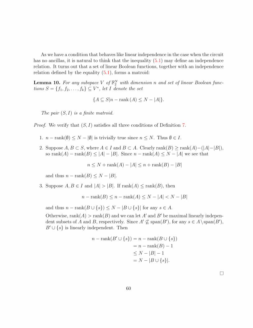
As we have a condition that behaves like linear independence in the case when the circuithas no ancillas, it is natural to think that the inequality (5.1) may define an independencerelation. It turns out that a set of linear Boolean functions, together with an independencerelation defined by the equality (5.1), forms a matroid:

Lemma 10. For any subspace V of FN2 with dimension n and set of linear Boolean func-tions S = {f1, f2, . . . , fk} ⊆ V ∗, let I denote the set

{A ⊆ S|n− rank (A) ≤ N − |A|}.

The pair (S, I) is a finite matroid.

Proof. We verify that (S, I) satisfies all three conditions of Definition 7.

1. n− rank(∅) ≤ N − |∅| is trivially true since n ≤ N . Thus ∅ ∈ I.

2. Suppose A,B ⊂ S, where A ∈ I and B ⊂ A. Clearly rank(B) ≥ rank(A)−(|A|−|B|),so rank(A)− rank(B) ≤ |A| − |B|. Since n− rank(A) ≤ N − |A| we see that

n ≤ N + rank(A)− |A| ≤ n+ rank(B)− |B|

and thus n− rank(B) ≤ N − |B|.

3. Suppose A,B ∈ I and |A| > |B|. If rank(A) ≤ rank(B), then

n− rank(B) ≤ n− rank(A) ≤ N − |A| < N − |B|

and thus n− rank(B ∪ {s}) ≤ N − |B ∪ {s}| for any s ∈ A.

Otherwise, rank(A) > rank(B) and we can let A′ and B′ be maximal linearly indepen-dent subsets of A and B, respectively. Since A′ 6⊆ span(B′), for any s ∈ A\ span(B′),B′ ∪ {s} is linearly independent. Then

n− rank(B′ ∪ {s}) = n− rank(B ∪ {s})= n− rank(B)− 1

≤ N − |B| − 1

= N − |B ∪ {s}|.

60

5.2.1 Matroid partitioning

The matroid partitioning problem can be defined as follows

Definition 8. (Matroid partitioning)

Given a matroid (S, I), find a partition {A1, A2, . . . , Ak} of S such that Ai ∈ I for each1 ≤ i ≤ k and for any other partition {A′1, A′2, . . . , A′k′} into independent subsets, k′ ≥ k.

Of particular interest is the fact that matroid partitioning can be solved in polynomialtime, given an independence oracle for the matroid [70]. As a consequence of Lemmas 9and 10, we see that the problem of finding a minimal partition of a set of linear Booleanfunctions into computable sets is reducible to the matroid partitioning problem, and thuscan be solved in polynomial time given an independence oracle. Since the condition inLemma 9 can be checked for a given subset A by using Gaussian elimination to computethe matrix rank, we thus see that a minimal partition of S into computable subsets canbe computed in polynomial time. Specifically, the independence test requires at most3,4

O(N3) time. The rest of this section describes an algorithm for computing a minimalpartition.

The algorithm we use for solving the matroid partitioning problem is based on analgorithm due to Edmonds [70]. Given a matroid (S, I) and a minimal (matroid) partitionP of S ′ ⊂ S, we take an element s ∈ S \ S ′ not already partitioned and construct aminimal partition of S ′ ∪ {s}. To create the new partition, we construct a directed graphGs containing a vertex u for every u ∈ S ′ ∪ {s} as well as a vertex ⊥p for every subsetp ∈ P . The edges of Gs represent changes to the partition that are invariant under theproperty of each subset being independent. In particular, for any u, v ∈ S ′ ∪ {s} thereis a directed edge v → u in Gs if and only if u is contained in some subset p ∈ P and(p \ {u}) ∪ {v} ∈ I, i.e. v can be added to p if we remove u. Additionally, given a subsetp ∈ P and element u ∈ S ′ ∪ {s}, there exists an edge u → ⊥p if and only if p ∪ {u} ∈ I.A path from s to ⊥p for some subset p gives a set of updates to P that produce a validpartition P ′ of S ′ ∪ {s}. Likewise, if there is no such path, there is no partition of size |P |partitioning S ′ ∪ {s} [70], and so a new subset {s} is added to P .

Rather than generating the graph Gs explicitly for each element s, we try to constructa path from s to some ⊥p breadth-first (Algorithm 5). It is well known that the time

3We can reduce this to O(n2N) in practice by storing vectors in V ∗ as length dim(V ) = n vectors. TheO(N3) bound is used for simplicity.

4Gaussian elimination cannot generally be bounded this way, as the representation of individual ele-ments may grow exponentially as rows get added together. Since our arithmetic is performed over thefinite field F2, we avoid this exponential blowup in the size of individual elements.

61

complexity of breadth-first search is O(|E|+|V |) for a graph with edge set E and vertices V .We can note that there are |S ′|+|P |+1 vertices and at most |S ′|2+|P |·(|S ′|+1)+(|S ′|+|P |)edges in Gs, as well as the fact that |P | ≤ |S ′|. Since each edge requires a single test forindependence in O(N3) time, the breadth first search requires time in O(|S ′|2 ·N3 + |S ′|).

Algorithm 5 Matroid partitioning algorithm

function Partition(s, P, (S, I))/* I denotes the independence oracle, P is a minimal partition */Create path queue Q, Q.enqueue(s→ ∅)Unmark each element of S, mark swhile Q non-empty do

t := Q.dequeue()for each A ∈ P do

Set A′ := A ∪ {head(t)}if A′ ∈ I then

Set A := A′

for each u→ v in path t doReplace u with v in its current partition

end forelse

for each unmarked u ∈ A doif A′ \ {u} ∈ I then

Q.enqueue(u→ t)Mark u

end ifend for

end ifend for

end whileIf no path was found, set P := P ∪ {s}

end function

Algorithm 5 details the algorithm for adding an element s to a partition P of matroid(S, I) – the full algorithm follows by iteratively adding each element of the ground set tothe initially empty partition, and correctness follows from the property that if P is minimalfor (S, I), then the new partition P ′ is minimal for (S ∪ {s}, I).

Since adding a single element to a partition of i elements takes O ((2i)2 ·N3 + 2i) time,

62

and∑|S|

i i2 = |S|33

+ |S|22

+ |S|6

, we see that Algorithm 5 can be used to partition the full setS of linear Boolean functions in O(|S|3 ·N3) time.

5.3 Towards a universal gate set

In the previous sections we described (in pieces) a method for re-synthesizing {CNOT, T}circuits while removing redundant T -gates and parallelizing the remaining ones. Specif-ically, given a circuit we can compute 〈S, g〉 and a new circuit computing U〈S,g〉 can besynthesized by first partitioning S into computable subsets using Algorithm 5, then com-pleting each subset by adding elements to make them reversible. Many efficient algorithmsexist [71, 14, 40] that can decompose the resulting linear reversible function into CNOTgates – in our implementation we use a Gaussian elimination algorithm – so that eachsubset can be computed, followed by a layer of T gates to apply the phase factors, thenuncomputed. To complete the procedure, we synthesize another linear reversible circuitcomputing g.

However, the usefulness of such an algorithm on its own is marred by the fact that{CNOT, T} circuits are an extremely restricted class of quantum circuits – in particular,they do not create superpositions or interference between basis states. To apply the opti-mization procedure to interesting quantum circuits, we have to extend these ideas to dealwith a universal gate set; this section details the different approaches we developed.

5.3.1 Embedded {CNOT, T} optimization

The most straightforward and obvious way of applying {CNOT, T} re-synthesis to a uni-versal gate set is to optimize only subcircuits. For instance, an optimization procedurecould traverse a circuit, gather the largest volume {CNOT, T} subcircuit that hasn’t yetbeen optimized, then replace it with the re-synthesized circuit. However, finding the largestvolume {CNOT, T} subcircuit is a non-trivial problem on its own, and each iteration wouldgenerally require traversing the whole circuit again, which we would like to avoid.

A slight relaxation to make such an algorithm more practical is to take a greedy ap-proach. In this approach, subcircuits are greedily constructed by traversing the circuit andrepeatedly adding {CNOT, T} gates to the current subcircuit until a non-{CNOT, T}gate occurs. The most glaring drawback is that T gates cannot commute across subcircuitboundaries, removing a great deal of optimization potential. For instance, the optimiza-tions in the motivating example (Figure 5.1) are no longer available, since Hadamard gates

63

separate the individual {CNOT, T} circuits corresponding to doubly controlled-Z gates –as the Λ2(Z) gates already have minimal T -depth and count, this effectively removes anypossibility of optimization.

Given this drawback, it is perhaps surprising that our experimental results in Section 5.5show very good performance on many arithmetic circuits. In fact, this method works verywell in circuits where nearby Toffolis do not mix control bits with target bits, since theHadamards can be pushed outwards in these cases. Moreover, a great deal of T gatereductions are available when adjacent Toffolis share controls and/or targets. As a result,embedding {CNOT, T} re-synthesis in general quantum circuits can be very effective undercertain conditions.

5.3.2 Abstract Hadamard gates

Motivated by the drawbacks of the embedded re-synthesis approach, we can consider waysto optimize directly over a universal gate set, specifically by extending the previous tech-niques to include Hadamard gates.

As in {CNOT, T} re-synthesis, the goal is to describe the phase factors in the outputas (linear Boolean) functions of an arbitrary input basis state. A new circuit can thenbe synthesized applying those phase factors as parallel as possible. In the embedding of{CNOT, T} re-synthesis into a universal gate set, each {CNOT, T} subcircuit is inter-preted as having a completely new input state, so the state space of any two subcircuitsis disjoint. We can do better by more accurately tracking the state space of different{CNOT, T} subcircuits, which would potentially allow phase factors to cancel and com-mute between them. To do so we need to know how the state space changes after applicationof a Hadamard gate.

We can observe that a Hadamard gate has the effect

H : |x〉 7→ 1√2

∑x′∈F2

(−1)x·x′|x′〉.

We call x′ a path variable, which represents two possible paths in the final state. Sincewe only want the effect of the Hadamard gate on the basis state, we drop the extraneousinformation5 and describe its action as

H ′ : |x〉 7→ |x′〉, x′ ∈ F2.

5The phase and magnitude are implicitly recovered in the synthesis procedure, so we do not need tokeep track of it.

64

In effect, a Hadamard gate destroys the qubit’s previous state and produces a new arbitrarystate. All the non-Hadamard phase factors in a {H,CNOT, T} circuit with N qubits andk Hadamard gates can then be described by c · f(x1, x2, ..., xN+k) for some linear Booleanfunction f and c ∈ Z8.

As an illustration, the Toffoli gate implementation in Figure 5.6 given the initial input|x1x2x3〉 generates two free variables x4, x5, shown in the figure. The total phase given bythe T gates can then be described as

ωx1+x2+x4+7·x1⊕x2+7·x1⊕x4+7·x2⊕x4+x1⊕x2⊕x4 .

The output state is then described as |x1x2x5〉. Furthermore, the state space before thefirst H, for example, is spanned by {x1, x2, x3}, so the phases conditioned on x1, x2, and7 · x1 ⊕ x2 could be applied before the first Hadamard when re-synthesizing, while all theother phases require x4 and thus must be applied before the second Hadamard gate.

x1 T • • T † • x1

x2 T • T † T † • x2

x3 Hx4

T • T • Hx5

x5

Figure 5.6: Clifford + T implementation of the Toffoli gate with the target on qubit 3.

As noted before, the abstraction H ′ is only used to more accurately describe the statespace of different sub-circuits, which are then individually re-synthesized; the differencefrom embedded {CNOT, T} optimization is that all phase factors are known at the sametime, so T gates in separate subcircuits can be combined and/or assigned to differentsubcircuits to further minimize T -depth. Specifically, after each Hadamard gate the statespace will be some subspace V of FN+k

2 , which is distinct from the subspace after any otherHadamard gate. Each function f(x1, x2, ..., xN+k) can then be computed in a subcircuitwith state space V if and only if f ∈ V ∗. The synthesis procedure can then decide in whichsubcircuit to apply each phase factor, in order to achieve efficient T -depth.

One approach to parsing out phase factors is to use the greedy nature of Algorithm 5 tomaintain a partition of those phase factors in S that are currently in the state space of thecircuit. We can iterate through the subcircuits, and for each one, partition any elements ofS that are not already partitioned and are in the state space of the subcircuit – this steprelies on the fact that Algorithm 5 is greedy to avoid having to partition everything againfrom scratch. As some of the partitioned functions may not be in the state space after the

65

next Hadamard gate, we then assign the phase factors in any partition block containingsuch a function to the current subcircuit and remove that block from the partition.

The process of removing partitions and partitioning new elements requires a closerlook to ensure that the partition is actually a minimal matroid partition at every step.Fortunately, it is straightforward to observe that any subset P ′ of a minimal matroidpartition P is also minimal for the remaining elements – if there existed a partition P0 ofthe elements in P ′ such that |P0| < |P ′|, then P0 ∪ P \ P ′ is a partition of the elements inP into fewer sets.

One problem arises in that the dimension of the state space may increase in the nextsubcircuit (e.g. if the Hadamard is applied to an ancilla qubit). In this case, the indepen-dence condition (5.1) of the matroid changes, and previous partitions may now be invalidunder the new inequality. However, as a trivial consequence of the fact that the dimensionincreases by at most 1, a partition that is no longer independent can be modified to satisfyit by removing exactly one element. Furthermore, if all partitions are modified to satisfythe new independence condition in this way, the new partition is minimal.

Lemma 11. Given a subspace V of FN2 with dimension n < N and a set of linear Booleanfunctions S ⊆ V ∗, let Ii = {A ⊆ S|i− rank (A) ≤ N − |A|}.

If P is some minimal partition of (S, In), then the partition P ′ defined by removingone linearly dependent element from every A ∈ P if A /∈ In+1 is a minimal partition of(S ′, In+1), where S ′ = ∪A∈PA is the set of elements partitioned by P ′.

Proof. Suppose there exists some partition P0 of (S ′, In+1) with |P0| < |P ′|.

We first see that one element of S \ S ′ can be added to any A ∈ P0 to give a setin In. In particular, consider any A ∈ P0. Since n + 1 − rank(A) ≤ N − |A| we seen−rank(A) ≤ N−|A|−1 = N−|A∪{s}|6 for any s ∈ S\S ′. Thus for any A ∈ P0, s ∈ S\S ′we have A ∪ {s} ∈ In.

Next we note that for any T ⊆ S there exists a partition of (T, In) with size at most|T | − 1. This is a simple result of the fact that n < N , as any subset A ⊆ T of size 2 hasrank at least 1, so n− rank(A) ≤ n− 1 ≤ N − 2 = N −|A|. Additionally, any size 1 subsetof T is trivially independent under In.

Thus since we can add one element to every partition in P0, and we can partition theremaining |S \ S ′| − |P0| elements into at most |S \ S ′| − |P0| − 1 partitions, we see that

6We also note that N − |A ∪ {s}| ≥ 0 as required, since any subset of S has rank at most n, i.e.∀A ∈ In+1, n + 1− rank(A) > 0 and thus |A| < N .

66

there exists a partition of (S, Im) with size at most |P0|+ (|S \S ′|− |P0|− 1) = |S \S ′|− 1.Since |S \ S ′| − 1 < |P | we obtain a contradiction.

5.3.3 Summing over paths

The last section implied a representation of {H,CNOT, T} circuits using linear Booleanfunctions with k free variables over FN+k

2 , but the Hadamard gates were left in place andonly their effect on the state space was tracked. We can instead re-synthesize the entirecircuit by fully describing the effect of a Hadamard gate,

H : |x〉 7→ 1√2

∑x′∈F2

ω4·x·x′ |x′〉,

leading to a complete algebraic representation of the circuit.

Lemma 12. If unitary U ∈ U(2N) is exactly implementable by an N-qubit circuit over{H,CNOT, T} with k H gates then for any computational basis state x1x2...xN ,

U : |x1x2...xN〉 7→1√2k

∑xN+1...xN+k∈Fk2

ωp(x1,x2,...,xN+k)|y1y2...yN〉

where yi = hi(x1, x2, . . . , xN+k) for some linear Boolean functions hi, and

p(x1, x2, ..., xN+k) =∑i

ci · fi(x1, x2, ..., xN+k) + 4 ·k∑i=1

xN+i · gi(x1, x2, ..., xN+k)

for some linear Boolean functions fi, gi and coefficients ci ∈ Z8.

Proof. Follows from the effect of each gate on the computational basis states.

Lemma 12 tells us that we can represent the unitary computed by a circuit over{H,CNOT, T} just with a polynomial p(x1, x2, ...,N+k ) in mixed arithmetic over Z2 andZ8, and a set of linear Boolean functions for the outputs y1, y2, ..., yN . A similar sum overpaths representation of this gate set was briefly discussed in [67] as a reduction from eval-uating quantum circuits to counting solutions to the polynomials. It’s worth noting thatunlike Lemma 8, the converse is not true – some polynomials will not correspond to aunitary transformation, as some are not even reversible. We leave testing of unitarity fora given expression of the type in Lemma 12 as an open question.

67

As in the last section, the synthesis procedure will have to make a “tour” through thevarious subspaces of FN+k

2 by applying Hadamard gates to instantiate the path variablesand pick up the phase factor ω4·xN+i·gi(x1,x2,...,xN+k). The difference is that the path is notfixed ahead of time, and so the synthesis procedure will need to reconstruct a sequence ofHadamard gates so that the circuit can transition through the state spaces and pick up eachphase factor. In doing so, it’s possible that an ordering that allows more parallelizationmay be chosen. We deal with the problem of choosing such a path in this section.

More precisely, we want to synthesize a {H,CNOT} skeleton of a full circuit imple-menting U , specifically the unitary

U0 : |x1x2...xN〉 7→1√2k

∑xN+1...xN+k∈Fk2

(−1)∑ki=1 xN+i·gi(x1,x2,...,xN+k)|y1y2...yN〉.

Once such a circuit is constructed we can add in the necessary phase factors betweenthe Hadamard gates using the same method as in Section 5.3.2. Additionally, we assumethat we are re-synthesizing a circuit, i.e. the polynomial p(x1, x2, ..., xN+k) and outputsy1, y2, ..., yN were generated from a real circuit. We leave open the question of synthesisfor arbitrary polynomial representations.

We begin by describing how to reconstruct the path from the original circuit, work-ing backwards from the output state. Let Vi ⊆ FN+k

2 be the state space of the originalcircuit after the ith Hadamard gate. Since xN+i ∈ Vi, we can choose a basis for Vi withrespect to the standard basis of FN+k

2 as Bi ∪ {xN+i}, where no vector in Bi containsxN+i. Furthermore, Bi ∪ {gi(x1, x2, ..., xN+k)} also forms a basis of Vi−1. Given N qubitsin states {b1, b2, ..., bN} forming a basis of Vi, we can then synthesize a circuit transform-ing the state space from Vi−1 to Vi and picking up the correct phase: we first synthesizeV : |b1b2...bN−1〉 7→

∣∣xN+ib′1...b

′N−1

⟩, where each of b′1, b

′2, ..., b

′N does not contain xN+i in

the standard basis, and then implement V †(H ⊗ I⊗N−1), which has the effect∣∣gi(x1, x2, ..., xN+k)b′1...b

′N−1

⟩7→ 1√

2

∑xN+i∈F2

(−1)xN+i·gi(x1,x2,...,xN+k)|b1b2...bN〉.

As the outputs {y1, y2, ..., yN} form a basis of Vk, we can thus synthesize a circuit imple-menting U ′ by iteratively synthesizing circuits transforming Vi−1 to Vi.

At the moment the only advantage of this synthesis method is that the circuit canbe more concisely represented using p(x1, x2, .., xN+k) and set of output functions with noimpact on the quality of the re-synthesized circuit. However, this method could also beused to parallelize or otherwise commute Hadamards as needed. Specifically, the method

68

works because the state space after every Hadamard contains at least one elementary vectorxN+i, and so we could create a basis diagonal in xN+i allowing a circuit to be synthesizedgenerating xN+i. If the state space contains more than one such elementary vector, wecould instead choose a basis that is diagonal in more than one path variable, and thusapply Hadamard gates in parallel. Care is still needed, as there may be phase factorsthat can only be computed between the Hadamard gates, but the flexibility to parallelizeHadamard gates could potentially lead to lower T -depths and lower total depths.

5.4 The Tpar algorithm

Up until now we’ve described the general ideas behind some T -gate optimization algorithms– in this section we present a concrete algorithm, Tpar, for optimizing T -count and depthin Clifford + T circuits, based on the representation described in Section 5.3.2. A versionof the algorithm optimizing just {CNOT, T} subcircuits, as described in Section 5.3.1, canbe constructed by applying Tpar to subcircuits between Hadamard gates.

Recall that in the computational basis, the input space of a circuit with N qubits, N−nancillas and k Hadamard gates is a dimension n subspace V of FN+k

2 . We required that allancillas are initialized in state |0〉. We represent the state of a qubit as a linear Booleanfunction f defined on FN+k

2 , or more succinctly as a vector in the dual space of FN+k2 ,

F(N+k)∗2 . In contrast to previous discussions we also maintain a Boolean value b specifying

the parity of the qubit, so that the full state is given by b⊕ f(x1, x2, ..., xN+k) – as we willsee, the parity corresponds to bit flips on the qubit.

Given a Clifford + T circuit C, written over G = {X, Y, Z, P, P †, H, CNOT, T, T †},we compute an abstraction 〈S,Q,H〉 of C where S = {(c, f)|c ∈ Z8, f ∈ F2 × F(N+k)∗

2 }represents the terms in the exponent of ω = ei

π4 as linear Boolean functions with a parity

bit and multiplicity, Q = (g1, g2, ..., gN), gi ∈ F2 × F(N+k)∗2 tracks the current state of each

qubit, and H = (h1, h2, ...hk) gives a list of Hadamard gates, where each Hadamard gatehi stores the input and output states, hi.QI and hi.QO respectively. We define the initialstate for the circuit as Q0 = ((0, x1), (0, x2), ..., (0, xn), (0, 0), ....), i.e. the first n qubitshave initial states |x1〉, |x2〉, ..., |xn〉 and the remainder are initialized as |0〉. To compute〈S,Q,H〉 we begin with 〈∅, Q0, ∅〉 and apply the updates shown in Figure 5.7 sequentiallyfor each gate in the circuit.

We define S ] T as the union of S and T where any f such that (c1, f) ∈ S, (c2, f) ∈ Tis assigned coefficient c1 + c2 mod 8. In this way phases applied to the same state areadded, potentially reducing the total number of T gates. Furthermore, we can note that

69

update(Xi, 〈S,Q,H〉) = 〈S,Q|gi:=¬gi , H〉update(Zi, 〈S,Q,H〉) = 〈S ] {(4, gi)}, Q,H〉update(Yi, 〈S,Q,H〉) = 〈S ] {(4, gi), (2,0)}, Q|gi:=¬gi , H〉update(Pi, 〈S,Q,H〉) = 〈S ] {(2, gi)}, Q,H〉update(P †i , 〈S,Q,H〉) = 〈S ] {(6, gi)}, Q,H〉

update(Hi, 〈S,Q, (h1, h2, ..., hi)〉) = 〈S,Q′, (h1, h2, ..., hi, {QI = Q,QO = Q′})〉where Q′ = Q|gi:=a|H|

update(CNOT(i,j), 〈S,Q,H〉) = 〈S,Q|gj :=gi⊕gj , H〉update(Ti, 〈S,Q,H〉) = 〈S ] {(1, gi)}, Q,H〉update(T †i , 〈S,Q,H〉) = 〈S ] {(7, gi)}, Q,H〉

Figure 5.7: Gate update rules. A gate Ui denotes gate U applied to qubit i, CNOT(i,j)

specifies i as the control qubit and j as the target.

bit flips on a state gi = (b, f) which naturally correspond to a negation of the stateb⊕ f(x1, x2, ..., xN+k) can be associated with the parity:

¬(b⊕ f(x1, x2, ..., xN+k)) = 1⊕ b⊕ f(x1, x2, ..., xN+k) = ¬b⊕ f(x1, x2, ..., xN+k).

So to apply a bit flip ¬gi, we change the parity of the qubit rather than allowing negativeoccurrences of variables in linear Boolean functions.

The Tpar algorithm (Algorithm 6) proceeds as follows: after computing 〈S,Q,H〉, weiterate through the Hadamard gates in H, updating a partition P of the functions of Sthat are computable in the current subcircuit. In particular, we divide S into SP and S−P ,where SP are the already partitioned elements and S−P are those not already partitioned.For a given hi = (QI , OO), we check whether f ∈ span(QI) for every (c, f) ∈ S−P , and ifso partition (c, f) using Algorithm 5 with the independence relation7

A ⊆ S ∈ I if and only if rank(QI)− rank(A) ≤ N − |A|.

After partitioning, we update SP and S−P accordingly.

7As before we implicitly lift the definition of rank for sets of linear Boolean functions to sets of linearBoolean functions with parity and coefficient.

70

Algorithm 6 T-parallelization algorithm

function Tpar(Clifford + T circuit C)Circuit:= ∅Compute 〈S,Q,H〉 for CSet SP := S; S−P := ∅; P := ∅for each 1 ≤ i ≤ k do

I := {A ⊆ S| rank(hi.QI)− rank(A) ≤ N − |A|}for each (c, f) ∈ S−P do

if f ∈ span(hi.QI) thenP :=Partition((c, f), P, (SP , I))SP := SP ∪ {(c, f)}; S−P := S−P \ {(c, f)}

end ifend forfor each A ∈ P do

if i = k or ∃(c, f) ∈ A such that f /∈ span(hi.QO) thenAppend(Circuit, Synthesize(A, hi.QI , hi.QI))P := P \ A

else if rank(hi.QO)− rank(A) > N − |A| thenChoose (c, f) ∈ A such that rank(A) = rank(A \ {(c, f)})A := A \ {(c, f)}; SP := SP \ {(c, f)}; S−P := S−P ∪ {(c, f)}

end ifend forAppend(Circuit, Synthesize(∅, hi.QI , hi.QO))

end forreturn Circuit

end function

We note that as per Section 5.2, the complexity of this step can be loosely bounded byO (|S−P | · (N + k)3 + |S|3 · (N + k)3). The actual run-time will be lower as the matriceson which we perform Gaussian elimination have dimension n + k × N , though we omit atighter analysis as the algorithm is heuristic in nature.

We next divide P into Pfrozen and Pfloat, where

Pfrozen = {A ∈ P |f /∈ span(QO) for some (c, f) ∈ A}Pfloat = P \ Pfrozen.

This step requires time in O (|SP | · (N + k)3). The names float and frozen imply that

71

the partitions can either float to the next subcircuit, or must be frozen in the currentone.

Once we have our partition Pfrozen, we construct a circuit computing the relevant phasefactors by taking each set A ∈ P , synthesizing a CNOT circuit computing A, applyingthe necessary phase rotations, then uncomputing A. The general synthesis procedure isdefined in Algorithm 7 and we defer discussion of the procedure for the moment, but forthe purpose of analyzing complexity we claim that such a procedure takes O(|S| · (N +k)3)time.

Finally, for every A ∈ Pfloat, we check whether A is an independent set under the newindependence relation

A ⊆ S ∈ I if and only if rank(QO)− rank(A) ≤ N − |A|.

If A /∈ I, we remove a linearly dependent element from A and update SP and S−P accord-ingly. As |Pfloat| ≤ |S| this requires an additional O (|S| · (N + k)3) operations.

The entire algorithm, shown in Algorithm 6, thus runs in time

O(|C| ·N + k · |S|3 · (N + k)3

).

As |C| ·N is in most cases negligible compared to the k · |S|3(N + k)3 factor, we can leaveit out and describe the run-time as simply O (k · |S|3 · (N + k)3) . Moreover, it should benoted that if no repartitioning is done, the run-time is bounded by O (|S|3 · (N + k)3) , aseach element is partitioned exactly once, rather than the worst case of k times in general.

5.4.1 Extended {CNOT, T} synthesis

As mentioned above, the Tpar algorithm relies on a procedure to synthesize a circuitapplying a (computable) set of phase factors A ⊆ S; we give pseudocode for a generalprocedure in Algorithm 7. Given input and output states for the qubits, QI and QO

respectively, SYNTHESIZE(A,QI , QO) returns a circuit implementing

U : |QI〉 7→ ω∑

(c,(b,f))∈A c·b⊕f(x1,x2,...,xN+k)|QO〉.

The synthesis proceeds by first addingN−|A| linear Boolean functions so that the resultingset A′ has rank equal to rank(QI) – this can be accomplished by using row operations toreduce A to a subset of QI , then adding the missing vectors. Next we synthesize a circuitcomputing A′ by reducing QI and A′ to the same basis using Gaussian elimination in

72

Algorithm 7 Extended {CNOT, T} synthesis

function Synthesize(A,QI , QO)/* Synthesize a {CNOT,X, T} circuit with inputs QI , outputs QO, and phases A */Compute A′ ⊇ A s.t. rank(A′) = rank(QI), |A′| = n+mSynthesize {CNOT,X} circuit C1 computing |QI〉 7→ |A′〉Synthesize {Z, P, T} circuit C2 computing |A′〉 7→ ω

∑(c,b,f)∈A′ c·b⊕f(x1,x2,...,xN+k)|A′〉

Synthesize {CNOT,X,H} circuit C3 computing |A′〉 7→ |QO〉Return C1C2C3

end function

O((N + k)3) time, where addition of two rows corresponds to the application of a CNOTgate, and parity changes correspond to X gates. The circuit reducing QI to the basisis applied forwards, while the circuit reducing A′ is applied in reverse, giving a circuitmapping |QI〉 7→ |A′〉. The phase factors are applied by constructing a combination ofT, P and Z gates, corresponding to the relevant coefficients, then a similar process ofGaussian elimination is used to compute |A′〉 7→ |QO〉. In the case when QO produces anew variable, the required Hadamard gate is also applied.

As |A| ≤ |S| we see that this step has time complexity O(|S| · (N + k)3), and assumingthe target fault tolerant architecture admits logical P and Pauli-Z gates, the T -depth ofthe resulting circuit is given by |A|.

This synthesis algorithm brings up an important practical issue. Our Gaussian elimina-tion based implementation produces circuits that are non-optimal in terms of the numberof gates or depth, resulting in a potential increase in the number of CNOT gates. Whileour focus was on the optimization of T gates, there exist algorithms, [40, 14], that producemore efficient circuits for linear reversible functions. Specifically, [14] provides an algo-rithm to synthesize linear reversible circuits with Θ(n2/ log(n)) gates, and [40] reports anO(n)-depth algorithm. More recently, [72] described an optimization procedure for linearreversible circuits that could be used to produce better circuits. In practical implementa-tions, one of these methods should be used instead of Gaussian elimination.

73

5.5 Results

We implemented8 Algorithm 6 in C++ and applied it to optimize various quantum, specif-ically arithmetic, circuits from the literature. Individual circuits were written in the stan-dard fault-tolerant universal gate set G = {X, Y, Z,H, P, CNOT, T}, using the decompo-sitions found in Chapter 4 where applicable. In particular, as most arithmetic circuitsare dominated by Toffoli gates, we used a T -depth 3 implementation of the Toffoli gate(Figure 4.14).

Our first implementation included only {CNOT, T} re-synthesis, which we appliedto Clifford + T circuits by optimizing only {CNOT, T} subcircuits as described in Sec-tion 5.3.1. For comparison between the two approaches, we ran experiments where Tparwas run only on subcircuits between Hadamard gates, as well as experiments using Tparto optimize the whole circuit.

Results are reported in Tables 5.1 and 5.2. They were generated in Debian Linuxrunning on a quad-core 64-bit Intel Core i5 2.80GHZ processor and 16 GB RAM. Table 5.1gives gate counts for the circuits. Table 5.2 focuses on T -depth using either 0, N , or ∞ancillas9 where N denotes the original number of qubits. The T -depth for each circuitbefore optimization was computed by parallelizing the T -gates and Toffoli gates by hand,and writing each group of parallel Toffoli gates in T -depth 3. As an example of a non-trivialcircuit, we show the initial (Figure 5.8) and Tpar optimized (Figure 5.9) circuits for the6-bit Cuccaro adder [2].

The benchmarks (Tables 5.1 and 5.2) show that when applying Tpar to {CNOT, T}subcircuits, the performance is strongly affected by the structure of the original circuit.In particular, the algorithm optimizes circuits where adjacent Toffoli gates share eithercontrols or targets, in which case the {CNOT, T} sub-circuits within the Toffolis can becombined. Each of the GF(2m) multipliers shares this structure. In fact, the Tpar algo-rithm with or without Hadamard gates can parallelize any GF(2m) multiplication circuitto T -depth 2 using sufficient ancillas, by noting that each such circuit can be written intwo {CNOT, T} stages. Those circuits that mix controls and targets between adjacentToffoli gates are less affected by the optimization, e.g., CSUM-MUX9, as the {CNOT, T}sub-circuits are separated by H gates.

By contrast, when Tpar is used to optimize the whole circuit, all the tested benchmarkshave significant reductions in terms of both T -count and depth. While the addition of

8The implementation is available at http://code.google.com/p/tpar/.9N was chosen as an arbitrary non-constant number of ancilla qubits to illustrate the trade off between

ancillas and T -depth.

74

Figure 5.8: 6-bit Cuccaro adder without expanding Toffoli gates [2].

Hadamards makes the algorithm more complex, the running time is not significantly sloweron any of the tested benchmarks, and T reduction and parallelization is better in all cases,providing strong evidence that abstracting Hadamard gates is a more effective way ofdealing with universal gate sets – in fact, running time was reduced by more than 50%in the large benchmarks. The results themselves show that there are great opportunitiesfor reducing T -count and depth in circuits, with average reductions of 40.7% and 57.8%respectively for the tested benchmarks. Combined with the fact that the algorithm scalesfavourably to large circuits, Tpar is an effective algorithm for the large-scale optimizationof fault tolerant circuits.

We also tested our algorithm’s ability to make use of ancillas to optimize T -depth(Table 5.2). For each of the benchmark circuits, we applied our algorithm with an addedN ancillas, where the original circuit contained N qubits. We also report the minimumT -depth achievable for each circuit using our algorithm. It can be noted that our algorithmusually decreases in running time when ancillas are added, due to the reduced number ofpartitions and thus faster matroid partitioning. Specifically, when there are many ancillas,for the majority of the time when an item s is partitioned it can be directly added toone of the partitions in time O(|P | · (N + k)3). As a result, the algorithm is very flexibleand capable of exploiting ancillas to reduce T -depth. Furthermore, our experimental dataillustrates a great potential for space-time trade-off in quantum circuits.

As a final remark, we note that our algorithm reproduces many of the previous re-

75

Figure 5.9: Optimized circuit from Figure 5.8 after expanding Toffolis. T -count was re-duced from 77 to 63 and T -depth was reduced from 33 to 27.

76

sults regarding the optimization of T -depth. In particular, Figure 5.10 shows the circuitproduced by running Tpar on an implementation of the Toffoli gate. The circuit mirrorsthe T -depth 1 Toffoli reported in [20]. Moreover, the full range of T -depths possible withdifferent numbers of ancillas can be observed, as in Figure 5.11.

Figure 5.10: T -depth 1 implementation of the Toffoli gate.

Figure 5.11: T -depth 2 implementation of the Toffoli gate.

We can further observe that other gates as computed in Chapter 4 can be parallelizedby adding ancillas and applying Tpar – for instance, the T -depth 1 controlled-P and -Vgates, as well as the controlled-T gate as shown in Figure 5.12. The Λ3(X) gate used inthe motivating example (Figure 5.1) can also be reduced to T -count 16 and T -depth 8(Figure 5.13), achieving lower T -count and -depth than the manual optimizations.

Figure 5.12: T -depth 3 implementation of the controlled-T gate.

5.6 Conclusions

We have described a closely related class of algorithms for re-synthesizing Clifford + T cir-cuits with reduced T -count and depth. These algorithms use representations of circuits by

77

Figure 5.13: Λ3(X) gate.

sets of linear Boolean functions, which allows T gates to be combined and then parallelizedby using Matroid theory to partition the functions into invertible subsets. The main algo-rithm, Tpar, has run-time cubic in the number of T gates, qubits, and Hadamard gates,though our experiments show that the algorithm is sufficiently fast for practical circuitsizes.

Our benchmarks (Tables 5.1 and 5.2) show that large gains can be made in reducingthe T -count and depth of quantum circuits. In some cases, T -count was reduced by 65.7%,while T -depth could be reduced by up to 86.7%. Furthermore, the benchmarks illustratethat ancillas can be used to parallelize T gates further, and given the run-times reportedthe algorithm can be seen to provide substantial flexibility in exploring the trade-off be-tween ancilla usage and T -depth. While the benchmarks demonstrated were all arithmeticor otherwise reversible operations, such operations typically require the majority of theresources in circuits for real quantum algorithms anyway.

5.6.1 Future work

As a major consequence of the Tpar algorithm, reducing the number of Z8 terms in themixed arithmetic polynomials describing the phase corresponds directly to reducing theT -complexity of circuits. In fact, for circuits not containing Hadamard gates, Tpar returnsa circuit of minimal T -count and depth if the phase function cannot be reduced. A naturalavenue for future work is then to develop methods for optimizing such polynomials for T -count and depth – we conjectured that finding the exact optimal expression is intractable,though in practice there may be good heuristics or approximation algorithms.

Sum over path style representations may also prove useful in optimizing circuits overother gate sets, or optimizing circuits for different costs. They provide a very succinct andcomputationally efficient way of representing the action of a quantum circuit, as opposedto quantum circuits or unitary matrices, neither of which reveal as much of the alge-braic structure of a computation. In particular, these representations appear particularlyamenable to circuit synthesis, and so an interesting problem would be to consider the gen-eration of the polynomial equations directly from unitaries, for instance those over the ring

78

Z[

1√2, i]. Combined with Tpar, multi-qubit unitaries could then be directly synthesized

with optimized T gates.

Finally, it may be useful to consider more advanced strategies for assigning phase gatesto regions of the circuit. As an example, it can be shown that Λm(X) for m > 3 can beimplemented in T -depth 2(m − 1) if partial results are not uncomputed – however, ouralgorithm produces circuits with T -depth 2(m−1)+1 as a result of the heuristic used. Aneffective area of further research would be to develop heuristics for generating partitionsthat result in better distributions of phase gates between Hadamard separated regions.

79

Benchmark N xC xT xg Time (s) x′C x′T x′g T -count reduction (%)

Mod 54 [73] 5 32 28 9 0.001 48 22 10 21.40.001 40 16 13 42.9

VBE-Adder3 [74] 10 80 70 20 0.001 94 40 15 42.90.002 80 24 23 65.7

CSLA-MUX3 [75] 15 90 70 20 0.002 189 64 23 8.60.003 219 62 21 11.4

CSUM-MUX9 [75] 30 196 196 84 0.011 242 112 172 42.90.018 222 110 152 43.9

QCLA-Com7 [76] 24 215 203 73 0.004 340 185 53 8.90.012 282 95 168 53.2

QCLA-Mod7 [76] 26 441 413 132 0.012 777 361 102 12.60.025 717 249 230 39.7

QCLA-Adder10 [76] 36 273 238 86 0.010 450 218 52 8.40.038 482 162 73 31.9

Adder8 [77] 24 466 399 126 0.010 792 315 134 21.10.016 646 215 230 46.1

RC-Adder6 [2] 14 104 77 30 0.002 161 77 30 0.00.004 167 63 61 18.2

Mod-Red21 [78] 11 121 119 58 0.004 230 119 53 0.00.005 192 73 110 38.7

Mod-Mult55 [78] 9 55 49 36 0.001 100 47 19 4.10.002 104 37 53 24.5

Λ3(X) [1] 5 28 28 8 0.001 48 28 6 0.00.001 38 16 12 42.9

Λ4(X) [1] 7 56 56 16 0.002 96 56 10 0.00.002 72 28 23 50.0

Λ5(X) [1] 9 84 84 24 0.002 144 84 14 0.00.002 106 40 34 52.4

Λ10(X) [1] 19 224 224 64 0.005 384 224 34 0.00.007 276 100 89 55.4

GF(24)-Mult [79] 12 115 112 32 0.004 262 76 29 32.10.005 245 68 27 39.3

GF(25)-Mult [79] 15 179 175 50 0.012 490 115 40 34.30.009 452 111 36 36.6

GF(26)-Mult [79] 18 257 252 72 0.027 830 162 49 35.70.020 759 150 43 40.5

GF(27)-Mult [79] 21 349 343 98 0.048 1143 217 56 36.70.044 1060 217 36 36.7

GF(28)-Mult [79] 24 468 448 128 0.111 1773 280 60 37.50.078 1591 264 40 41.1

GF(29)-Mult [79] 27 575 567 162 0.235 2184 351 64 38.10.143 1886 351 44 38.1

GF(210)-Mult [79] 30 709 700 200 0.420 3022 430 71 38.60.279 2402 410 69 41.4

GF(216)-Mult [79] 48 1856 1792 512 8.353 8994 1072 122 40.24.257 8657 1040 82 42.0

GF(232)-Mult [79] 96 7291 7168 2048 770.369 49230 4192 246 41.5370.400 41796 4128 166 42.4

GF(264)-Mult [79] 192 28860 28672 8192 92236.729 273977 16576 494 42.243979.598 214941 16448 334 42.6

Average 21.940.7

Maximum 42.965.7

Table 5.1: Gate count benchmarks. N specifies the number of qubits. xC reports thenumber of CNOT gates, xT gives the number of T gates, and xg gives the number of othergates. x′ denotes the number of gates after optimization by Tpar on subcircuits withoutH gates (first row), and on the whole circuit (second row).

80

Benchmark T -depth T -depth Red. Time T -depth Red. Time T -depth Red.original 0 ancilla (%) (s) N ancilla (%) (s) ∞ ancilla (%)

Mod 54 [73] 12 9 25.0 0.001 4 66.7 0.001 3 75.07 41.7 0.001 4 66.7 0.001 3 75.0

VBE-Adder3 [74] 24 15 37.5 0.001 5 79.2 0.001 5 79.211 54.2 0.001 5 79.2 0.001 5 79.2

CSLA-MUX3 [75] 21 10 52.4 0.001 4 81.0 0.001 4 81.07 66.7 0.003 4 81.0 0.003 4 81.0

CSUM-MUX9 [75] 18 12 33.3 0.004 5 72.2 0.004 3 83.312 33.3 0.010 5 72.2 0.01 3 83.3

QCLA-Com7 [76] 27 21 22.2 0.004 9 66.7 0.004 7 74.114 48.1 0.009 7 74.1 0.008 7 74.1

QCLA-Mod7 [76] 57 42 26.3 0.007 16 71.9 0.007 14 75.430 47.4 0.020 15 73.7 0.019 14 75.4

QCLA-Adder10 [76] 24 17 29.2 0.005 7 70.8 0.004 6 75.012 50.0 0.017 7 70.8 0.016 6 75.0

Adder8 [77] 69 44 36.2 0.007 16 76.8 0.007 15 78.333 52.2 0.015 16 76.8 0.014 15 78.3

RC-Adder6 [2] 33 33 0.0 0.002 11 66.7 0.002 11 66.727 18.2 0.003 11 66.7 0.003 11 66.7

Mod-Red21 [78] 48 40 16.7 0.003 15 68.8 0.006 15 68.830 37.5 0.004 15 68.8 0.005 15 68.8

Mod-Mult55 [78] 15 9 40.0 0.001 4 73.3 0.002 4 73.39 40.0 0.002 4 73.3 0.002 4 73.3

Λ3(X) [1] 12 12 0.0 0.001 4 66.7 0.001 4 66.79 25.0 0.001 4 66.7 0.001 4 66.7

Λ4(X) [1] 24 24 0.0 0.001 8 66.7 0.002 8 66.717 29.2 0.001 8 66.7 0.001 8 66.7

Λ5(X) [1] 36 36 0.0 0.002 12 66.7 0.003 12 66.725 30.6 0.002 12 66.7 0.002 12 66.7

Λ10(X) [1] 96 96 0.0 0.004 32 66.7 0.013 32 66.765 32.3 0.006 32 66.7 0.01 32 66.7

GF(24)-Mult [79] 36 9 75.0 0.002 5 86.1 0.002 2 94.47 80.6 0.003 4 88.9 0.003 2 94.4

GF(25)-Mult [79] 48 10 79.2 0.004 5 89.6 0.002 2 95.89 81.3 0.006 5 89.6 0.005 2 95.8

GF(26)-Mult [79] 60 11 81.7 0.011 6 90.0 0.003 2 96.711 81.7 0.011 5 91.7 0.007 2 96.7

GF(27)-Mult [79] 72 13 81.9 0.029 7 90.3 0.004 2 97.212 83.3 0.028 7 90.3 0.011 2 97.2

GF(28)-Mult [79] 84 15 82.1 0.049 7 91.7 0.005 2 97.613 84.5 0.041 7 91.7 0.014 2 97.6

GF(29)-Mult [79] 96 16 83.3 0.114 8 91.7 0.007 2 97.915 84.4 0.085 7 92.7 0.028 3 96.9

GF(210)-Mult [79] 108 18 83.3 0.311 9 91.7 0.008 2 98.117 84.3 0.216 8 92.6 0.038 2 98.1

GF(216)-Mult [79] 180 27 85.0 7.681 13 92.8 0.025 2 98.924 86.7 2.715 12 93.3 0.18 2 98.9

GF(232)-Mult [79] 372 51 86.3 1340.412 24 93.5 0.186 2 99.551 86.3 266.300 24 93.5 2.678 2 99.5

GF(264)-Mult [79] 756 101 86.6 268472.634 46 93.9 2.573 2 99.7104 86.2 46950.853 48 93.7 87.604 2 99.7

Average 45.7 78.9 82.957.8 79.5 82.9

Maximum 86.6 93.9 99.786.7 93.9 99.7

Table 5.2: T -depth benchmarks. We report the T -depth after no optimization (original),and after optimization with 0 (i.e. Table 5.1), N , or unbounded ancillas.

81

APPENDICES

82

Appendix A

Complexity of T -count minimization

This thesis has largely been concerned with the problem of minimizing T -count in quantumcircuits. In this section we formalize a conjecture made earlier regarding the complexity ofa T -count minimization problem.

In Chapter 5 it was mentioned that the {CNOT, T} circuit re-synthesis algorithmdoesn’t necessarily find the minimal T -count (and by extension, T -depth) to implement agiven unitary using CNOT and T (†), P (†), or Z gates. Finding an expression of the circuit’sphase as a polynomial over Z2 and Z8 minimizing the number of odd coefficients was shownto be equivalent to minimizing T -count. Here we formally state the conjecture that thisproblem is NP-hard.

Conjecture 1. For a sequence (ak)k∈{0,1}n , ak ∈ Z8, define the polynomial p(ak)(x1, x2, ..., xn)as

p(ak)(x1, x2, ..., xn) =∑

k∈{0,1}nak · (xk11 ⊕ xk22 ⊕ · · · ⊕ xknn ).

Given a sequence (ak)k∈{0,1}n , ak ∈ Z8, the problem of finding some sequence (bk)k∈{0,1}n , bk ∈Z8 such that p(ak)(x1, x2, ..., xn) = p(bk)(x1, x2, ..., xn) for all x1, x2, ..., xn ∈ {0, 1} minimiz-ing

∑k∈{0,1}n(bk mod 2) is NP-hard.

We describe the phase polynomial in slightly different, more general terms here – partic-ularly, each term xk11 ⊕xk22 ⊕· · ·⊕xknn is a linear Boolean function of the inputs x1, x2, ..., xn.The connection to minimization of T -count, described in Chapter 5, is in the minimization∑

k∈{0,1}n(bk mod 2), as each odd coefficient in the phase requires one T gate to imple-

ment. Since every polynomial of the form p(ak)(x1, x2, ..., xn) defines the global phase forsome {CNOT, T} circuit, the two minimization problems are informally equivalent.

83

References

[1] A. Barenco, C. H. Bennett, R. Cleve, D. P. DiVincenzo, N. Margolus, P. Shor,T. Sleator, J. A. Smolin, and H. Weinfurter, “Elementary gates for quantum com-putation,” Phys. Rev. A, vol. 52, pp. 3457–3467, Nov 1995, quant-ph/9503016.

[2] S. A. Cuccaro, T. G. Draper, S. A. Kutin, and D. Petrie Moulton, “A new quantumripple-carry addition circuit,” ArXiv e-prints, Oct. 2004, quant-ph/0410184.

[3] V. Kabanets and J.-Y. Cai, “Circuit minimization problem,” in Proceedings of thethirty-second annual ACM symposium on Theory of computing, STOC ’00, (New York,NY, USA), pp. 73–79, ACM, 2000.

[4] R. K. Brayton, A. L. Sangiovanni-Vincentelli, C. T. McMullen, and G. D. Hachtel,Logic Minimization Algorithms for VLSI Synthesis. Norwell, MA, USA: Kluwer Aca-demic Publishers, 1984.

[5] J. W. Britton, B. C. Sawyer, A. C. Keith, C.-C. J. Wang, J. K. Freericks, H. Uys,M. J. Biercuk, and J. J. Bollinger, “Engineered two-dimensional ising interactions in atrapped-ion quantum simulator with hundreds of spins,” Nature, no. 7395, p. 489492,2012.

[6] K. R. Brown, A. C. Wilson, Y. Colombe, C. Ospelkaus, A. M. Meier, E. Knill,D. Leibfried, and D. J. Wineland, “Single-qubit-gate error below 10−4 in a trappedion,” Phys. Rev. A, vol. 84, p. 030303, Sep 2011, arXiv:1104.2552.

[7] J. M. Chow, J. M. Gambetta, A. D. Corcoles, S. T. Merkel, J. A. Smolin, C. Rigetti,S. Poletto, G. A. Keefe, M. B. Rothwell, J. R. Rozen, M. B. Ketchen, and M. Steffen,“Universal quantum gate set approaching fault-tolerant thresholds with superconduct-ing qubits,” Phys. Rev. Lett., vol. 109, p. 060501, Aug 2012, arXiv:1202.5344.

84

[8] C. Rigetti, J. M. Gambetta, S. Poletto, B. L. T. Plourde, J. M. Chow, A. D. Corcoles,J. A. Smolin, S. T. Merkel, J. R. Rozen, G. A. Keefe, M. B. Rothwell, M. B. Ketchen,and M. Steffen, “Superconducting qubit in a waveguide cavity with a coherence timeapproaching 0.1 ms,” Phys. Rev. B, vol. 86, p. 100506, Sep 2012, arXiv:1202.5533.

[9] H. Bombin, R. S. Andrist, M. Ohzeki, H. G. Katzgraber, and M. A. Martin-Delgado,“Strong resilience of topological codes to depolarization,” Phys. Rev. X, vol. 2,p. 021004, Apr 2012, arXiv:1202.1852.

[10] A. G. Fowler, A. M. Stephens, and P. Groszkowski, “High-threshold universal quan-tum computation on the surface code,” Phys. Rev. A, vol. 80, p. 052312, Nov 2009,arXiv:0803.0272.

[11] A. G. Fowler, A. C. Whiteside, and L. C. L. Hollenberg, “Towards practical classicalprocessing for the surface code,” Phys. Rev. Lett., vol. 108, p. 180501, May 2012,arXiv:1110.5133.

[12] O. Golubitsky and D. Maslov, “A study of optimal 4-bit reversible toffoli circuits andtheir synthesis,” Computers, IEEE Transactions on, vol. 61, no. 9, pp. 1341–1353,2012, arXiv:1103.2686.

[13] W. N. N. Hung, X. Song, G. Yang, J. Yang, and M. Perkowski, “Optimal synthesisof multiple output boolean functions using a set of quantum gates by symbolic reach-ability analysis,” Computer-Aided Design of Integrated Circuits and Systems, IEEETransactions on, vol. 25, no. 9, pp. 1652–1663, 2006.

[14] K. N. Patel, I. L. Markov, and J. P. Hayes, “Optimal synthesis of linear reversiblecircuits,” Quantum Info. Comput., vol. 8, pp. 282–294, Mar. 2008, quant-ph/0302002.

[15] D. Maslov, G. W. Dueck, D. M. Miller, and C. Negrevergne, “Quantum circuit sim-plification and level compaction,” Trans. Comp.-Aided Des. Integ. Cir. Sys., vol. 27,pp. 436–444, Mar. 2008, quant-ph/0604001.

[16] R. Dias da Silva, E. Pius, and E. Kashefi, “Global quantum circuit optimization,”ArXiv e-prints, Jan. 2013, arXiv:1301.0351.

[17] A. Paetznick and A. G. Fowler, “Quantum circuit optimization by topological com-paction in the surface code,” ArXiv e-prints, Apr. 2013, arXiv:1304.2807.

85

[18] M. Amy, D. Maslov, M. Mosca, and M. Roetteler, “A meet-in-the-middle algorithmfor fast synthesis of depth-optimal quantum circuits,” Computer-Aided Design of In-tegrated Circuits and Systems, IEEE Transactions on, vol. 32, no. 6, pp. 818–830,2013, arXiv:1206.0758.

[19] A. Bocharov and K. M. Svore, “Resource-optimal single-qubit quantum circuits,”Phys. Rev. Lett., vol. 109, p. 190501, Nov 2012, arXiv:1206.3223.

[20] P. Selinger, “Quantum circuits of T -depth one,” Phys. Rev. A, vol. 87, p. 042302, Apr2013, arXiv:1210.0974.

[21] C. Jones, “Low-overhead constructions for the fault-tolerant toffoli gate,” Phys. Rev.A, vol. 87, p. 022328, Feb 2013, arXiv:1212.5069.

[22] A. G. Fowler, “Time-optimal quantum computation,” ArXiv e-prints, Oct. 2012,arXiv:1210.4626 [quant-ph].

[23] R. Landauer, “Information is physical,” in Physics and Computation, 1992. PhysComp’92., Workshop on, pp. 1–4, 1992.

[24] P. Kaye, R. Laflamme, and M. Mosca, An Introduction to Quantum Computing. Ox-ford University Press, 2007.

[25] P. Shor, “Algorithms for quantum computation: discrete logarithms and factoring,”in Foundations of Computer Science, 1994 Proceedings., 35th Annual Symposium on,pp. 124–134, 1994, quant-ph/9508027v2.

[26] S. Lloyd, “Universal quantum simulators,” Science, vol. 273, no. 5278, pp. 1073–1078,1996.

[27] M. Nielsen and I. Chuang, Quantum Computation and Quantum Information. Cam-bridge Series on Information and the Natural Sciences, Cambridge University Press,2000.

[28] A. Y. Kitaev, A. H. Shen, and M. N. Vyalyi, Classsical and Quantum Computation.Graduate studies in mathematics, v. 47, American mathematical society, 2002.

[29] D. Gottesman, “The heisenberg representation of quantum computers,” in Inter-national Conference on Group Theoretic Methods in Physics, p. 9807006, 1998,quant-ph/9807006v1.

86

[30] V. Kliuchnikov, D. Maslov, and M. Mosca, “Fast and efficient exact synthesis of singlequbit unitaries generated by Clifford and T gates,” Quantum Info. Comput., vol. 13,pp. 607–630, July 2013, arXiv:1206.5236.

[31] B. Giles and P. Selinger, “Exact synthesis of multiqubit Clifford+T circuits,” Phys.Rev. A, vol. 87, p. 032332, Mar 2013, arXiv:1212.0506.

[32] D. P. DiVincenzo, “Two-bit gates are universal for quantum computation,” Phys. Rev.A, vol. 51, pp. 1015–1022, Feb 1995, cond-mat/9407022.

[33] A. Y. Kitaev, “Quantum computations: algorithms and error correction,” RussianMathematical Surveys, vol. 52, pp. 1191–1249, Dec. 1997.

[34] W. K. Wootters and W. H. Zurek, “A single quantum cannot be cloned,” Nature,vol. 299, p. 802, Oct. 1982.

[35] A. Paetznick and B. W. Reichardt, “Universal fault-tolerant quantum computa-tion with only transversal gates and error correction,” ArXiv e-prints, Apr. 2013,arXiv:1304.3709.

[36] D. Gottesman and I. L. Chuang, “Quantum teleportation is a universal computationalprimitive,” Nature, no. 6760, p. 390393, 1999, quant-ph/9908010.

[37] S. Bravyi and A. Kitaev, “Universal quantum computation with ideal clifford gatesand noisy ancillas,” Phys. Rev. A, vol. 71, p. 022316, Feb 2005, quant-ph/0403025.

[38] D. Gottesman, “Theory of fault-tolerant quantum computation,” Phys. Rev. A,vol. 57, pp. 127–137, Jan 1998, quant-ph/9702029.

[39] A. Broadbent and E. Kashefi, “Parallelizing quantum circuits,” Theor. Comput. Sci.,vol. 410, pp. 2489–2510, June 2009, arXiv:0704.1736.

[40] D. Maslov, “Linear depth stabilizer and quantum fourier transformation circuits withno auxiliary qubits in finite-neighbor quantum architectures,” Phys. Rev. A, vol. 76,p. 052310, Nov 2007, quant-ph/0703211.

[41] M. Saeedi, R. Wille, and R. Drechsler, “Synthesis of quantum circuits for linear nearestneighbor architectures,” Quantum Information Processing, vol. 10, no. 3, pp. 355–377,2011, arXiv:1110.6412.

87

[42] M. Mottonen, J. J. Vartiainen, V. Bergholm, and M. M. Salomaa, “Quantum cir-cuits for general multiqubit gates,” Phys. Rev. Lett., vol. 93, p. 130502, Sep 2004,quant-ph/0404089.

[43] V. Shende, A. Prasad, I. Markov, and J. Hayes, “Synthesis of reversible logic circuits,”Computer-Aided Design of Integrated Circuits and Systems, IEEE Transactions on,vol. 22, no. 6, pp. 710–722, 2003, quant-ph/0207001.

[44] D. Maslov and D. Miller, “Comparison of the cost metrics through investigation of therelation between optimal NCV and optimal NCT three-qubit reversible circuits,” Com-puters Digital Techniques, IET, vol. 1, no. 2, pp. 98–104, 2007, quant-ph/0511008.

[45] A. G. Fowler, “Constructing arbitrary Steane code single logical qubit fault-tolerantgates,” Quantum Info. Comput., vol. 11, pp. 867–873, Sept. 2011, quant-ph/0411206.

[46] D. Grosse, R. Wille, G. Dueck, and R. Drechsler, “Exact multiple-control toffoli net-work synthesis with SAT techniques,” Computer-Aided Design of Integrated Circuitsand Systems, IEEE Transactions on, vol. 28, no. 5, pp. 703–715, 2009.

[47] C. M. Dawson and M. A. Nielsen, “The Solovay-Kitaev algorithm,” Quantum Info.Comput., vol. 6, pp. 81–95, Jan. 2006, quant-ph/0505030.

[48] P. Selinger, “Efficient Clifford+T approximation of single-qubit operators,” ArXive-prints, Dec. 2012, arXiv:1212.6253.

[49] V. Kliuchnikov, D. Maslov, and M. Mosca, “Practical approximation of single-qubitunitaries by single-qubit quantum Clifford and T circuits,” ArXiv e-prints, Dec. 2012,arXiv:1212.6964.

[50] A. K. Prasad, V. V. Shende, I. L. Markov, J. P. Hayes, and K. N. Patel, “Data struc-tures and algorithms for simplifying reversible circuits,” J. Emerg. Technol. Comput.Syst., vol. 2, pp. 277–293, Oct. 2006.

[51] D. Miller, D. Maslov, and G. Dueck, “A transformation based algorithm for reversiblelogic synthesis,” in Design Automation Conference, 2003. Proceedings, pp. 318–323,2003.

[52] D. Maslov, G. Dueck, and D. Miller, “Toffoli network synthesis with templates,”Computer-Aided Design of Integrated Circuits and Systems, IEEE Transactions on,vol. 24, no. 6, pp. 807–817, 2005.

88

[53] M. Sedlk and M. Plesch, “Towards optimization of quantum circuits,” Central Euro-pean Journal of Physics, vol. 6, no. 1, pp. 128–134, 2008, quant-ph/0607123.

[54] C. Moore and M. Nilsson, “Parallel quantum computation and quantum codes,” SIAMJ. Comput., vol. 31, pp. 799–815, Mar. 2002, quant-ph/9808027.

[55] R. Raussendorf and H. J. Briegel, “Computational model underlying the one-wayquantum computer,” Quantum Info. Comput., vol. 2, pp. 443–486, Oct. 2002,quant-ph/0108067.

[56] D. E. Browne and H. J. Briegel, “One-way quantum computation - a tutorial intro-duction,” ArXiv e-prints, Mar. 2006, quant-ph/0603226.

[57] S. Aaronson and D. Gottesman, “Improved simulation of stabilizer circuits,” Phys.Rev. A, vol. 70, p. 052328, Nov 2004, quant-ph/0406196.

[58] T. Bozkaya and M. Ozsoyoglu, “Indexing large metric spaces for similarity searchqueries,” ACM Trans. Database Syst., vol. 24, pp. 361–404, Sept. 1999.

[59] P. N. Yianilos, “Data structures and algorithms for nearest neighbor search in gen-eral metric spaces,” in Proceedings of the fourth annual ACM-SIAM Symposium onDiscrete algorithms, SODA ’93, (Philadelphia, PA, USA), pp. 311–321, Society forIndustrial and Applied Mathematics, 1993.

[60] N. Kumar, L. Zhang, and S. Nayar, “What is a good nearest neighbors algorithm forfinding similar patches in images?,” in Computer Vision ECCV 2008 (D. Forsyth,P. Torr, and A. Zisserman, eds.), vol. 5303 of Lecture Notes in Computer Science,pp. 364–378, Springer Berlin Heidelberg, 2008.

[61] S. Sen and R. E. Tarjan, “Deletion without rebalancing in balanced binary trees,”in Proceedings of the Twenty-First Annual ACM-SIAM Symposium on Discrete Al-gorithms, SODA ’10, (Philadelphia, PA, USA), pp. 1490–1499, Society for Industrialand Applied Mathematics, 2010.

[62] P. Pham, “Quantum compiler,” 2011.

[63] A. M. Childs, R. Cleve, E. Deotto, E. Farhi, S. Gutmann, and D. A. Spielman,“Exponential algorithmic speedup by a quantum walk,” in Proceedings of the thirty-fifth annual ACM symposium on Theory of computing, STOC ’03, (New York, NY,USA), pp. 59–68, ACM, 2003, quant-ph/0209131.

89

[64] A. Peres, “Reversible logic and quantum computers,” Phys. Rev. A, vol. 32, pp. 3266–3276, Dec 1985.

[65] R. P. Feynman, “Quantum mechanical computers,” Foundations of Physics, vol. 16,no. 6, pp. 507–531, 1986.

[66] M. Amy, D. Maslov, and M. Mosca, “Polynomial-time T -depth optimizationof Clifford+T circuits via matroid partitioning,” ArXiv e-prints, Mar. 2013,arXiv:1303.2042.

[67] C. M. Dawson, A. P. Hines, D. Mortimer, H. L. Haselgrove, M. A. Nielsen, and T. J.Osborne, “Quantum computing and polynomial equations over the finite field Z2,”Quantum Info. Comput., vol. 5, pp. 102–112, Mar. 2005, quant-ph/0408129.

[68] T. Rudolph, “Simple encoding of a quantum circuit amplitude as a matrix permanent,”Phys. Rev. A, vol. 80, p. 054302, Nov 2009, arXiv:0909.3005.

[69] R. P. Feynman and A. R. Hibbs, Quantum mechanics and path integrals. Internationalseries in pure and applied physics, McGraw-Hill, 1965.

[70] J. Edmonds, “Minimum partition of a matroid into independent subsets,” JournaB1lof Research of the National Bureau of Standards, vol. 69B, pp. 67–72, Jan. 1965.

[71] T. Beth and M. Roetteler, “Quantum algorithms: Applicable algebra and quantumphysics,” in Quantum Information, vol. 173 of Springer Tracts in Modern Physics,pp. 96–150, Springer Berlin Heidelberg, 2001.

[72] V. Kliuchnikov and D. Maslov, “Optimization of Clifford circuits,” ArXiv e-prints,May 2013, arXiv:1305.0810.

[73] D. Maslov, “Reversible logic synthesis benchmarks page,” 2011.

[74] V. Vedral, A. Barenco, and A. Ekert, “Quantum networks for elementary arithmeticoperations,” Phys. Rev. A, vol. 54, pp. 147–153, Jul 1996, quant-ph/9511018.

[75] R. Van Meter and K. M. Itoh, “Fast quantum modular exponentiation,” Phys. Rev.A, vol. 71, p. 052320, May 2005, quant-ph/0408006.

[76] T. G. Draper, S. A. Kutin, E. M. Rains, and K. M. Svore, “A logarithmic-depthquantum carry-lookahead adder,” Quantum Info. Comput., vol. 6, pp. 351–369, July2006, quant-ph/0406142.

90

[77] Y. Takahashi, S. Tani, and N. Kunihiro, “Quantum addition circuits and unboundedfan-out,” Quantum Info. Comput., vol. 10, pp. 872–890, Sept. 2010, arXiv:0910.2530.

[78] I. L. Markov and M. Saeedi, “Constant-optimized quantum circuits for modular mul-tiplication and exponentiation,” Quantum Info. Comput., vol. 12, pp. 361–394, May2012, arXiv:1202.6614.

[79] D. Maslov, J. Mathew, D. Cheung, and D. K. Pradhan, “An O(m2)-depth quantumalgorithm for the elliptic curve discrete logarithm problem over GF(2m),” QuantumInfo. Comput., vol. 9, pp. 610–621, July 2009, arXiv:0710.1093.

[80] P. Aliferis, D. Gottesman, and J. Preskill, “Quantum accuracy threshold for con-catenated distance-3 codes,” Quantum Info. Comput., vol. 6, pp. 97–165, Mar. 2006,quant-ph/0504218.

[81] A. Parent, J. Parker, M. Burns, and D. Maslov, “QCViewer: a tool for displaying,editing, and simulating quantum circuits,” 2013.

[82] X. Zhou, D. W. Leung, and I. L. Chuang, “Methodology for quantum logic gateconstruction,” Phys. Rev. A, vol. 62, p. 052316, Oct 2000, quant-ph/0002039.

91