I

Thanks

Thanks to the f. b. of my underwater hockey comrades, for letting me beat them during the

training while I was writing this thesis; for excluding me from most social medias, to avoid

me distractions; for insulting me for my delays and my confusion between the right and the

left side.

Thanks to D. and M. that inspired me the formulation of the “universal energetic Theory”

based on resonances and able to explain each type of human sensation and to allow to

identify the proper filter as shield to avoid it and protect yourself. We are nothing but light

and pulsing electromagnetic waves.

Thanks the a. pilot E. Lo Greco, helped me to correct this thesis and to integrate it with

aeronautical and flights notions.

Thanks to my Austrian underwater rugby comrades, with who I played a lot of nice matches

in Austria.

Thanks to Toronto raptors basketball team of colleagues for the basketball matches and the

beers drank together.

Thanks to Clean Sky JU in which environment this work was thought and devolopped.

III

Synthesis

In this thesis are considered two of the biggest problem of the civil aircraft, such as the bad

weather avoidance and the fuel consumption and emission reduction, and a possible

solution, based on the trajectory optimization, is proposed.

The goal of this work is to propose a method to develop a trajectory optimizer, suitable to run

in real time on an on-board device, that provide the pilot with a decision support system,

helping him in trajectory optimization for weather avoidance and emission reduction.

In the first part of the thesis the framework is described in terms of European Authorities

goals, to reduce aircraft fuel consumption and emissions, and weather phenomenon

dangerous for the aircraft flight. An overview of the devices available in aeronautics to detect

and predict weather conditions is then provided. In the next chapter an analysis of civil

aircraft categories, trajectory, flight phases and flight planning is provided to characterize the

object of the optimization (aircraft trajectory). Then different kind of algorithms and method

for trajectory optimization are described and compared. In the next chapter our graph based

approach for multi-object trajectory optimization is proposed and details about the models

used, to generate the graph of feasible trajectories from a certain aircraft in a certain volume

of the airspace, are described. Then the results of such a trajectory optimizer applied to real

flights in unforeseen weather conditions are provided. Finally, a method to automatically

generate the minimum graph of feasible trajectory useful to produce, in real time, an

optimized trajectory with a minimum computational time is defined and tested in four use

cases.

1

Contents Index

THANKS .............................................................................................................................................. I

SYNTHESIS .................................................................................................................................... III

CONTENTS INDEX ......................................................................................................................... 1

FIGURE INDEX ................................................................................................................................ 5

TABLES INDEX ................................................................................................................................ 7

CHAPTER 1 INTRODUCTION .................................................................................................... 9

1.1 THESIS STRUCTURE ..................................................................................................................... 10

CHAPTER 2 WEATHER PHENOMENA OVERVIEW ...................................................... 13

2.2 CLIMATOLOGY AND INTERCHANGE OF METEOROLOGICAL INFORMATION ................................. 13

2.3 WEATHER PHENOMENA IMPACTING ON AVIATION .................................................................... 16

2.3.1 Thunderstorms ................................................................................................................. 16

2.3.1.1 Thunderstorm Stages .................................................................................................... 17

2.3.1.2 Thunderstorm Types .................................................................................................... 17

2.3.1.3 Air Mass Thunderstorm ............................................................................................... 18

2.3.1.4 Severe Thunderstorm ................................................................................................... 18

2.3.1.5 Squall-Line Thunderstorm .......................................................................................... 18

2.3.1.6 Hazards with thunderstorms ...................................................................................... 19

2.3.2 Lightning ........................................................................................................................... 19

2.3.3 Downburst ........................................................................................................................ 20

2.3.4 Wind Shear ....................................................................................................................... 21

2.3.5 Tornado ............................................................................................................................. 22

2.3.6 Hail ..................................................................................................................................... 22

2.3.7 Airframe Icing .................................................................................................................. 22

2.4 WEATHER MODELS FOR AERONAUTICAL APPLICATIONS ............................................................ 22

2

2.4.1 Global versions ................................................................................................................. 23

2.5 DEVICES USED TO DETECT WEATHER PHENOMENON ................................................................ 25

2.5.1 Onboard information sources ........................................................................................ 26

2.5.1.1 Pressure .......................................................................................................................... 27

2.5.1.2 Temperature .................................................................................................................. 27

2.5.1.3 Multi-function probe .................................................................................................... 27

2.5.1.4 Humidity ........................................................................................................................ 28

2.5.1.5 Onboard Weather radar .............................................................................................. 28

2.5.2 On ground information sources .................................................................................... 31

CHAPTER 3 OVERVIEW ON CIVIL AIRCRAFT FLIGHT ........................................... 33

3.1 AIRCRAFT CATEGORIES ............................................................................................................... 33

3.2 PHASE OF FLIGHT ....................................................................................................................... 34

3.2.1 Taxing ................................................................................................................................ 34

3.2.2 Take-off ............................................................................................................................. 35

3.2.3 Climb .................................................................................................................................. 36

3.2.4 Cruise ................................................................................................................................. 37

3.2.5 Descent .............................................................................................................................. 37

3.2.6 Landing ............................................................................................................................. 38

3.3 FLIGHT PLANNING ..................................................................................................................... 39

3.3.1 Commercial flight procedures........................................................................................ 40

3.3.1.1 Lateral profile ................................................................................................................ 41

3.3.1.2 Vertical profile - SID & STAR...................................................................................... 41

CHAPTER 4 OVERVIEW ON ALGORITHMS FOR TRAJECTORY

OPTIMIZATION ............................................................................................................................. 43

4.1 REVIEW OF THE LITERATURE ..................................................................................................... 43

4.2 ALGORITHMS FOR TRAJECTORY OPTIMIZATION ........................................................................ 46

4.2.1 The typical terminology for trajectory optimization ................................................. 46

4.2.2 Trajectory optimization techniques .............................................................................. 48

4.2.2.1 Single shooting .............................................................................................................. 48

4.2.2.2 Multiple shooting ......................................................................................................... 48

4.2.2.3 Direct collocation ......................................................................................................... 49

4.2.2.4 Orthogonal collocation ................................................................................................ 49

4.2.2.5 Pseudospectral collocation ......................................................................................... 49

4.2.2.6 Differential dynamic programming ......................................................................... 49

4.2.3 Comparison of techniques .............................................................................................. 50

4.2.3.1 Indirect vs. direct methods .......................................................................................... 50

3

4.2.3.2 Shooting vs. collocation ............................................................................................... 50

4.2.3.3 Mesh refinement: h vs. p ............................................................................................. 51

4.2.4 Graph theory .................................................................................................................... 51

4.2.5 Ant Colony ......................................................................................................................... 51

CHAPTER 5 OUR APPROACH: DJIKSTRA GRID FOR AIRCRAFT

TRAJECTORY OPTIMIZATION AND MODELS USED ................................................... 52

5.1 MODELS DESCRIPTION ................................................................................................................ 52

5.1.1 Emissions model ................................................................................................................ 53

5.1.1.1 The Boeing 2 Method ..................................................................................................... 53

5.1.2 Effects of meteorological changes .................................................................................. 54

5.1.3 Noise Model ....................................................................................................................... 55

5.1.4 Weather data ..................................................................................................................... 56

5.1.5 Aircraft model ................................................................................................................... 57

5.1.6 Graph construction .......................................................................................................... 58

5.1.6.1 Graph construction (base of data of feasible trajectories) ...................................... 59

5.1.6.2 Dijkstra based trajectory optimizer ........................................................................... 62

5.1.6.3 Genetic based trajectory optimizer ............................................................................ 63

5.1.6.4 Multi-objective trajectory optimization .................................................................... 64

5.1.6.5 Generation of Non-dominated solutions: Pareto ..................................................... 64

CHAPTER 6 RESULTS OF TRAJECTORY OPTIMIZER APPLIED TO REAL

SCENARIOS WITH UNFORESEEN WEATHER EVENTS .............................................. 66

6.1 WEATHER PREDICTION RELIABILITY .......................................................................................... 67

6.1.1 evaluation of weather prediction Accuracy.................................................................. 68

6.1.1.1 Reflectivity forecast accuracy ...................................................................................... 69

6.1.1.2 Wind forecast accuracy ................................................................................................ 72

6.2 TRAJECTORY OPTIMIZATION TEST CASES ................................................................................... 72

6.2.1 Test Case 1 ......................................................................................................................... 72

6.2.1.1 Meteorological data ...................................................................................................... 73

6.2.1.2 Route and aircraft emissions ...................................................................................... 73

6.2.1.3 Test results ..................................................................................................................... 75

6.2.2 Test Case 2 ........................................................................................................................ 76

6.2.2.1 Meteorological data ...................................................................................................... 76

6.2.2.2 Route and aircraft emissions ...................................................................................... 77

6.3 TRAJECTORY OPTIMIZATION WITH EMISSIONS WEIGHTS .......................................................... 79

6.3.1 Meteorological data ......................................................................................................... 79

6.3.2 Route and aircraft emissions ......................................................................................... 80

4

6.3.3 Comparing multi-objective trajectories using Pareto front ..................................... 82

6.4 TRAJECTORY OPTIMIZATION WITH DIFFERENT WEATHER MODEL AND EMISSIONS WEIGHTS .. 86

6.4.1 Meteorological data......................................................................................................... 86

6.4.2 Route and aircraft emissions ......................................................................................... 87

6.4.3 Comparison of emissions associated to optimized trajectory using Pareto .......... 88

6.4.4 Comparison of pollutant emissions using different atmospheric information RAP

(real weather data), ISA data and RAP without wind ........................................................ 90

6.5 DATA VALIDATION IN X-PLANE FLIGHT SIMULATOR ................................................................. 91

CHAPTER 7 MINIMUM SIZE GRAPH GENERATION AND RESULTS ................. 94

7.1 AUTOMATICALLY GRAPH GENERATION ...................................................................................... 94

7.2 EXPERIMENTAL SET UP .............................................................................................................. 95

7.2.1 Test cases characterization ............................................................................................. 95

7.2.1.1 Test cases 3 ..................................................................................................................... 96

7.2.1.2 Test cases 2 Graph generation .................................................................................... 97

7.2.1.3 Test cases 1 Graph generation .................................................................................... 98

7.2.1.4 Test cases 4 ..................................................................................................................... 99

7.2.2 Computational Method applied ................................................................................... 100

7.2.3 Software implementation ............................................................................................. 101

7.3 TESTS RESULTS ........................................................................................................................ 103

CHAPTER 8 CONCLUSIONS .................................................................................................. 105

ACRONYMS ................................................................................................................................... 107

REFERENCES ............................................................................................................................... 110

5

Figure Index

Fig1 Thunderstorm Development 17

Fig2 Severe Thunderstorm 19

Fig3 Charge Separation 20

Fig.4 Example of Probes location in an A380 26

Fig.5 Example of A380 Multi-Function Probes 28

Fig.6 Anatomy of a cumulonimbus 30

Fig.7 representation of aircraft trajectory with the different phases of flight 34

Fig.8 aircraft phases of flight and emissions target to be reduced 35

Fig.9 Complete trajectory for an aircraft from takeoff to landing 40

Fig.10 Descent profile for a commercial aircraft 42

Fig.11 Effect of pressure on emission index of NOx 54

Fig.12 Aircraft trajectory with A320 typical performance parameters (maximum and Minimum

speed, altitude, climb time and distance) 62

Fig.13 Weather reflectivity on USA the 18/6/2012 at 3 a.m 69

Fig.14 Real and forecasted reflectivity on USA the 18/6/2012 at 3 a.m 70

Fig.15 Real and forecasted reflectivity above 20 dBz on USA the 18/6/2012 at 3 a.m 70

Fig.16 Comparison Real (analysis, cyan) and forecasted (1h before) reflectivity 71

Fig.17 The Wind speed, direction and intensity (different colors) at 10668 m. 73

Fig.18 DAL1888 real flights (black one usual, red one particular deviation tested) 74

Fig.19 DAL1888 real flights (black one usual, red one tested) 74

Fig.20 Real trajectory (black) performed by DAL1888 and optimized trajectories (waypoints

blue and red) 76

Fig.21 The Wind speed, direction and intensity (different colors) at 3000 m. 77

Fig.22 The Wind speed, direction and intensity (different colors) at 8000 m. 77

Fig.23 Two trajectories performed by DAL1760 in different days and atmospheric conditions

are reported. 78

Fig.24 The Wind speed, direction, and intensity (different colors) at 3000 m. 80

Fig.25 The Wind speed, direction, and intensity (different colors) at 8000 m. 80

6

Fig.26 Two trajectories performed by DAL1451 in different days and atmospheric conditions

are reported. 81

Fig.27 The Wind speed, direction (arrows) and intensity (more colors) at 5000 m 86

Fig.28 Two trajectories performed by NKS724 in different days and atmospheric conditions

are reported 87

Fig.29 X-plane flight simulator in which is visible the selected aircraft (A320) flight along the

optimized trajectory (in pink in the picture) uploaded in FMS. 92

Fig.30 X-plane flight simulator cockpit view of the selected A320 92

Fig.31 MARS weather radar simulator display in which the cloud reflectivity is visualized 93

Fig.32 Block scheme of the software implementation 101

7

Tables Index

Table 1 Extract from Air France A330/340 operations manual

Table 2 Clouds reflectivity prediction reliability

Table 8 Initial and final position of DAL1451 trajectory considered

Table 9 estimated emissions of DAL1451 in different atmospheric conditions

Table 10 DAL1451 emissions and emission associated to optimized trajectories

Table 11 Emissions associated to multi-object Dijkstra optimized trajectories

8

Table 12 Emissions associated to multi-object Genetic optimized trajectories

Table 13 Initial and final position aircraft position

Table 14 estimated emissions of NKS724 in different atmospheric conditions

Table 15 NKS724 emissions and emission associated to optimized trajectories

Table 16 Emissions associated to multi-object Djikstra optimized trajectories for

different set of emission weights

Table 17 Emissions associated to mono-object (CO2, NOx, Nose) optimized

trajectories calculated with real weather condition (from RAP), ISA standard

atmospheric condition and RAP data without wind

Table 18 Initial waypoint position, speed and heading for the analyzed test cases

Table 19 Final waypoint position, speed and heading for the analyzed test cases

Table 20 Graph computation with different resolution and emissions associated to

the trajectory optimized with different optimization objectives.

Table 21 Graph computation with different resolution and emissions associated to

the trajectory optimized with different optimization objectives.

Table 22 Graph computation with different resolution and emissions associated to

the trajectory optimized with different optimization objectives.

Table 23 Graph computation with different resolution and emissions associated to

the trajectory optimized with different optimization objectives.

9

Table 24 Exel file generated by the Matlab program for the automatic grid

generation in which all useful parameters are contained.

Table 25 Test cases results in term of graph dimension, computational time,

iterations, and trajectory emissions

10

CHAPTER 1

INTRODUCTION

The growth experienced by the air transport at a global level in recent years has been

translated finally into an increase in the emissions of atmospheric polluting agents, which

conflicts with the requirement of reducing the global level of emissions.

The air traffic is expected to triple its size worldwide within 2020, in comparison to year

2000. Huger air traffic means also a greater environmental impact: the increase in number

of flights will increase air pollution and level of perceived noise on the ground. Air traffic is

estimated to contribute about 3-6% to global warming considering the combined impacts of

emissions of CO2, NOx and water vapour. Emission of CO2 and of other air pollutants from

air traffic globally is estimated to increase by about 5% per year [5].

From Vision 2020 Report [1] onwards, the Advisory Council for Aeronautics Research in

Europe (ACARE) recognized the environment as a major challenge for European Aeronautics

and Air Transport, then recommending a total commitment in minimizing the impact on the

global environment and confirming this goal in the first edition of the Strategic Research

Agenda 1 (SRA-1) [2], in the second updated edition (SRA-2) [3] and in the 2008 Addendum

to the Strategic Research Agenda.

As a technological response to such recommendations, the European Commission created

the 7th Framework (FP7) Clean Sky Joint Technology Initiative for funding large scale and

long term partnerships to implement ambitious and complex activities requiring very huge

public and private investments and human resources. Clean Sky, through the validation at a

high readiness level, aims at demonstrating the technology breakthroughs necessary to make

major steps towards ACARE goals [1,2,3] to be reached in 2020 for the avionic sector.

On the other side weather, especially related to convection, is responsible worldwide for large

delays and widespread disruptions especially in the periods of year when travel demand is

11

higher [4]. Weather-induced impacts account for 70% of all delays, with convective weather

accounting for 60% of all weather-related delays [5]. Time and location of fast-evolving

phenomena like thunderstorms are often very difficult to predict. Because of its

unpredictability, weather is the largest contributor to delays over the air traffic control

system and is a major factor in aircraft safety incidents and accidents [6].

For the previous motivations, it has been useful to develop a trajectory optimizer, for weather

avoidance and emission reduction, based on operational research algorithms, subject of this

thesis. In particular, in this thesis is proposed a method to optimize aircraft trajectory for

weather avoidance and emission reduction based on Dijkstra algorithm. To better

understand the contest, several fields have been taken into account and described here. First

of all in this thesis is provided a description of the meteorological models used in

aeronautical field and a definition of the dangerous weather condition that can affect the

flight. Then an overview of the algorithms for trajectory optimization is provided to have a

reference of the methodologies used to solve the same problem that we are considering. Later

a description of our trajectory optimization approach and the models used to implement it

are provided with some application results. In the following paragraph a method to improve

and speed up the trajectory optimization generation is proposed and some results are

provided. The proposed approach provides a methodology to optimize trajectory in terms of

weather avoidance and emission reduction and provide a solution in a fast and accurate way.

Such a problem depends of atmospheric conditions (humidity, pressure, temperature, wind,

clouds, …) and on the airspace in which it is possible to flight that is discretized in a grid of

feasible trajectories for a certain aircraft. In fact, in order to compute aircraft emissions, it is

required the atmospheric distribution, in altitude, of the following meteorological data:

density of air, pressure, temperature, relative humidity, wind intensity, speed and direction,

and clouds reflectivity. These data, except density of the air, are available through numerical

weather models that several weather organizations in the world develop for analysis of

current situations and forecasts.

Moreover, the determination of optimal aircraft trajectories has been of considerable interest

to civil aeronautics (ATC, aircraft companies, etc) for almost 50 years. Efforts were put in

trying to minimize fuel, time and more recently emissions and noise.

1.1 Thesis Structure

The thesis has the following structure:

Thanks

Synthesis

Content Index

12

Figure Index

Table Index

Introduction

Thesis Chapters

Conclusions

Bibliography

Annex

In Section 1 general the scope of this work is summarized. At last an overview of the overall

Thesis is given.

In Section 2 is provided an overview of the weather phenomena impacting on trajectory

optimization and the main meteorological information required and to be interchanged.

Moreover, in this section are also described weather phenomena that can be met during a

flight (thunderstorms, lightning, downburst, wind shear, tornado, hail, airframe icing) and it

is provided an example of what it is possible to detect, with onboard weather radar, in

presence of a cumulonimbus. Finally, an overview of the on board and on ground weather

information sources is provided.

In Section 3 is provided an overview civil aircraft categories and a description of the aircraft

trajectory, the different phases of flight and trajectory planning.

In Section 4, an overview of different algorithms for trajectory optimization, and a

comparison between them, is provided.

In Section 5 our trajectory optimization approach is described as well as the models used to

implement it (aircraft BADA model, ICAO model, ISA standard atmospheric model, GRIB

weather files, ...)

In Section 6, the results of the trajectory optimizer applied to real scenarios with unforeseen

weather events are provided

In Section 7 a method to generate a graph of minimum size, for a selected accuracy is

proposed and the calculation results are provided.

In Section 8 the conclusions are provided.

At the end of the thesis are reported the references and acronyms.

13

CHAPTER 2

WEATHER

PHENOMENA

OVERVIEW

The weather is the cause of approximately 70 percent of the aircraft delays. In addition,

weather continues to play a significant role in a number of aircraft trajectory modification

from the preplanned one. The total weather impact is an estimated national cost of $3 billion

for accident damage and injuries, delays, and unexpected operating costs [7].

Unforeseen, adverse weather (other than low visibility and runway condition) and

adverse wind conditions (i.e., strong cross winds, tailwind and wind shear) compel the pilot

to take sudden decisions regarding trajectory variations with few information, that often are

not sufficient to take the right decision in term of emission reduction (for the same safety).

In these cases, at present, for safety reason and luck of information, the pilot manages

the event without taking into account aircraft emissions, but only avoidance procedures. In

this contest, would be very useful a device able to provide to the pilot more information

about alternative safe trajectories taking into account both procedure to avoid the

phenomenon and pullant reduction.

2.2 Climatology and interchange of meteorological

information

Climatology is important in modern aviation because it studies the phenomenon associate

with atmospheric temperature, pressure, precipitation, solar radiation, winds, upper winds

14

and regional climatic environments in different parts of the world, but also particular local

meteorological phenomena that affect flying operations [13]. Moreover, climate considers the

parameters that mostly influence aircraft performance and emissions, in particular

temperature, pressure, humidity, wind and precipitation.

The important aspects of the atmosphere affecting the flight of an aircraft are the location

and nature of jet streams, areas of turbulence, location of storm clouds, and the low-level

weather for safe landing and take-off. These features of the weather are the result of dynamic

and thermal dynamic energy processes within the atmosphere, an understanding of which is

essential for the pilot.

On the other side, weather phenomenon are often unpredictable and weather models are not

so extremely accurate, so the preplanned trajectories, based on weather prediction,

sometimes have to be modified during the flight and update weather condition are required.

For this reason, in recent years, weather sensor systems and communication systems for

interchange of meteorological information have been improved.

Considering the nature of long haul aviation, pilots need forecasts of the main meteorological

phenomena that is required for planning the flight. They also need to understand upper

winds, temperatures, tropopause heights, jet streams, mountain waves, thunderstorm

activity, tropical cyclones, clear air turbulence (CAT), volcanic activity and such phenomena

when conducting the flight. Also, there is the terminal weather (TAFs - Terminal Air

Forecasts) and the airports nominated as alternates, both en-route and the destination [15].

Global weather forecasting is becoming a reality. The UK Meteorological Office (MO) is

developing its Numerical Weather Prediction (NWP) model, and the resolution of the areas

(grid squares) around the world is improving.

The World Area Forecast Centres (WAFCs) under the provision of ICAO, is centered at two

locations, the UK Met Office (Bracknell) and also Washington USA (based in Kansas City).

Three INTELSAT 604 satellites provide global coverage. The UK Met Office uses one at 60” E

(SADIS Satellite), and covers Europe, the Middle East and South Asia. The USA covers the

other half of the globe. The satellites are in geostationary orbit.

The MO produces charts of significant weather from Flight Level 100 to Flight Level 450 for

Europe and FL 450 to FL 630 for the North Atlantic. Also spot wind charts for the same

areas. Significant weather includes jet streams, heights, direction, and core speeds. The

significant weather charts and associated spot winds are produced from FL 250 to FL 450 for

the Middle East and South Asia.

Upper wind and temperature charts are produced for ten global regions, twice a day at nine

levels. Thus, the total output is 396 charts a day. Only the significant weather charts are

combined manually, the rest, E 360, are produced by automation.

The distribution of such charts presently is by the T4 FAX standard of 64 kbit/sec, but a new

format to be used is ‘GRIB’ binary. This is more suitable for transmission of Grid Point

15

Format charts. The GRIB code is contained in [10,11,15] and the GRIB format will allow

world atmosphere models to be transmitted, allowing airlines to optimize their tracks.

The MO increasingly relies on meteorological satellites to provide weather observations

particularly over the oceans. Aircraft will provide additional data, but the system will be

automated. British Airways will have over 60 aircraft supplying fully automated weather

reports. On average, the MO will receive 160 wind and temperature reports daily from each

operational aircraft and these are used directly in producing the NWP forecasts, which are

becoming the primary method of weather forecasting. This is done by solving a set of

equations. A computer model of the atmosphere shows how weather conditions will change

over time.

A valuable source of meteorological and climate observations is becoming available from the

new Quickscat satellite - on board is NASA’s SeaWinds instrument. Access to daily wind data

and animations from the ocean-wind tracker are managed by NASA’s Jet Propulsion

Laboratory (JPL), Pasadena, California.

The heart of SeaWinds is a specially designed spaceborne radar instrument called a

scatterometer. The radar operates at a microwave frequency that penetrates clouds. This,

coupled with the satellite’s polar orbit, makes the wind systems over the entire world’s

oceans visible on a daily basis. The measurements provide detailed information about ocean

winds, waves, currents, polar ice features and other phenomena, for the benefit of

meteorologists and climatologists [8,15].

This data will be used operationally by forecasters and for numerical weather prediction

models. Upper air observations are also obtained from suitably equipped ships on the

Atlantic shipping lanes. This system is presently becoming operational. The MO will receive

weather data twice a day for approximately 20 days of each voyage.

Aircraft fitted with the ACARS (Aircraft Communications and Reporting System) Teleprinter

system already receive Aircraft Operational Control (AOC), Airline Administrative Control

(AAC) and Air Traffic Control (ATC). The system is an air to ground data link system used on

HF, INMARSAT, and particularly VHF; however, HF, VHF and UHF frequencies are used.

The cockpit equipment consists of a small printer, although, if this fails, a read-out can be

seen on the alphanumeric display on the control unit. Through this system, pilots can be

alerted to anything unusual which affects the current flight segment. This may include

changing weather conditions, updating of TAFs, SIGMETs or mechanical information [8,15].

All these meteorological information, coming from different sources, should be processed,

fused and used to improve pilot information and support him in real time during the

onboard decisions.

16

2.3 Weather phenomena impacting on aviation

In the following sub paragraphs are described the weather phenomenon [14] that mostly

influence the aircraft performance and require to the pilot a sudden decision in the sense of

trajectories modification.

In particular, the following phenomenon are taken into account and described:

- Thunderstorms

- Lightning

- Turbulence (i.e. downburst)

- Wind shear

- Icing

- Hail

- Tornadoes

2.3.1 Thunderstorms

A thunderstorm is a cumulonimbus cloud that contains lightning and thunder. Strong wind

gusts, heavy rain, lightning, hail and tornadoes are typical hazards produced by

thunderstorms. They usually exist for only a short time, rarely over two hours for a single

storm.

The National Weather Service definition of a thunderstorm includes: “accompanied by

thunder and lightning” It must produce lightning to be labeled a thunderstorm. It must be

electrically active. Lightning is always present, in and near, a thunderstorm.

Thunderstorm development requires three elements:

1) Moisture

2) Lifting Agent

3) Instability

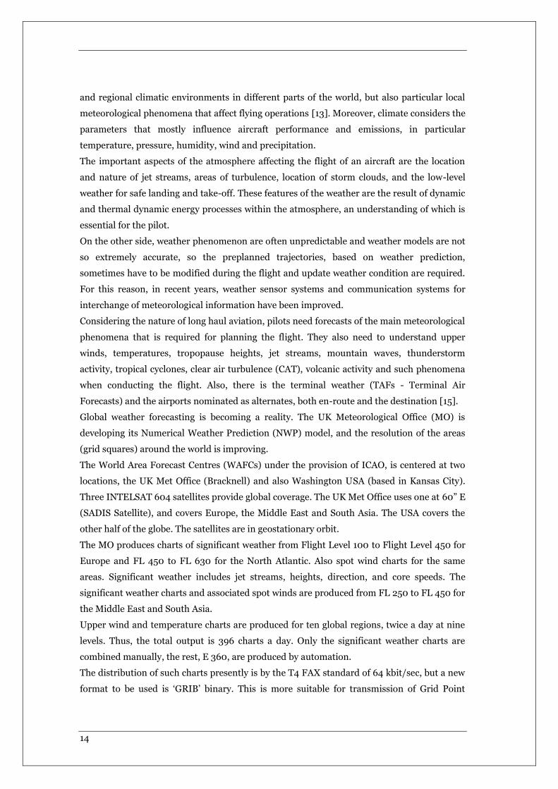
A cumulus cloud forms when moist air is lifted by a thermal, frontal, or orographic process. If

the atmosphere is unstable, the lifted air mass will continue to rise and develop into a

thunderstorm cell (Fig 1). As the building mass soars upwards, moisture condenses and

precipitation-induced downdrafts develop. This process creates violent wind shear and

turbulence, and lightning within the cell. Precipitation begins to fall from the cloud base, and

the thunderstorm is born.

17

Fig1 Thunderstorm Development

2.3.1.1 Thunderstorm Stages

The life cycle of a thunderstorm includes three stages: cumulus, mature, and dissipating.

Cumulus Stage — is the beginning of all thunderstorms. The size of the updraft region (cell)

becomes larger and the cloud grows in an unsteady succession of upward bulges, as evident

by the thermals that reach to the top. Strong vertical winds, severe turbulence, icing and

lightning, are typical hazards that an aircraft could encounter at this stage.

Mature Stage — is reached when the precipitation-induced downdraft reaches the ground.

Heavy rain or hail, and in colder areas sleet or snow, are driven by strong downdrafts. Wind

shear, lightning and thunder develop because of friction between the opposing air currents.

At this stage, the hazards can be devastating for any aircraft.

Dissipating Stage — is reached when the updraft is overwhelmed by the precipitation

induced downdraft. With no source of moisture, the associated hazards decrease and the

entire thunderstorm gradually dissipates.

2.3.1.2 Thunderstorm Types

There are several types of thunderstorms: The air mass thunderstorm, the severe

thunderstorm, and squall-line thunderstorm. An air mass thunderstorm consists of one cell

18

and lasts less than one hour, whereas the severe thunderstorm is composed of multi-cells or

supercells, and lasts for up to two hours.

2.3.1.3 Air Mass Thunderstorm

The Air Mass Thunderstorm grows quickly and is contained within a single cell. At

maturation, the thunderstorm is normally self-destructive. Updrafts elevate water. Water

accumulates in the upper areas of the storm. When the upward source can no longer support

the accumulated water mass, it rains. The rainfall (downward) overwhelms and strangles the

lifting process (upward), and the storm dissipates.

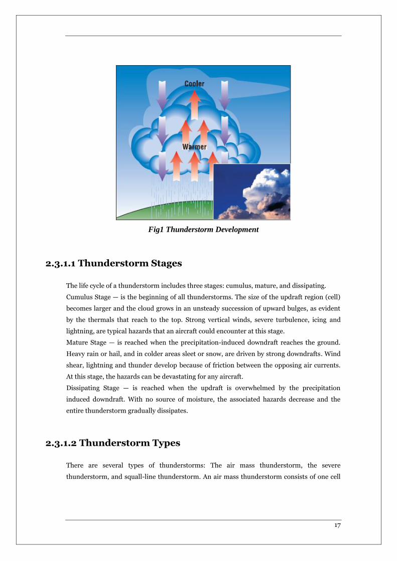
2.3.1.4 Severe Thunderstorm

The Severe Thunderstorm develops when a number of single cells interact and produce more

cells (multi cells), thus sustaining the life of the storm.

Specifically, the strong updraft tilts and twists moisture into the upper air support. With

strong upper atmosphere winds (for example, the Jet Stream,) the storm tilts or leans

downwind. This is evident by the highest portion of the cloud spreading outward

(downwind), and forming an anvil shape, fig 32. The water carried upward will accumulate

and rain downwind, possibly far ahead of the storm’s updraft core. Consequently, the mature

stage does not initiate the dissipating stage by strangling the updraft element.

A severe thunderstorm has a greater intensity than an air mass thunderstorm. This is evident

by the weather it produces: winds of 50 knots or greater, three-quarters of an inch or larger

destructive hail, and/or strong tornadoes.

2.3.1.5 Squall-Line Thunderstorm

Squall line storms are the most disruptive to aviation because they form in lines that can

stretch a few hundred miles, and individual storms in the lines can be fierce. Strictly

speaking, the lines of storms usually referred to as squall-lines are “pre-frontal squall-lines.”

Squall lines often trail large areas of stratus clouds with low ceiling and visibility that can

linger for hours.

19

Fig2 Severe Thunderstorm

2.3.1.6 Hazards with thunderstorms

A thunderstorm contains every conceivable aerial hazard: lightning, catastrophic turbulence,

wind shear, severe icing, destructive hail, and tornadoes.

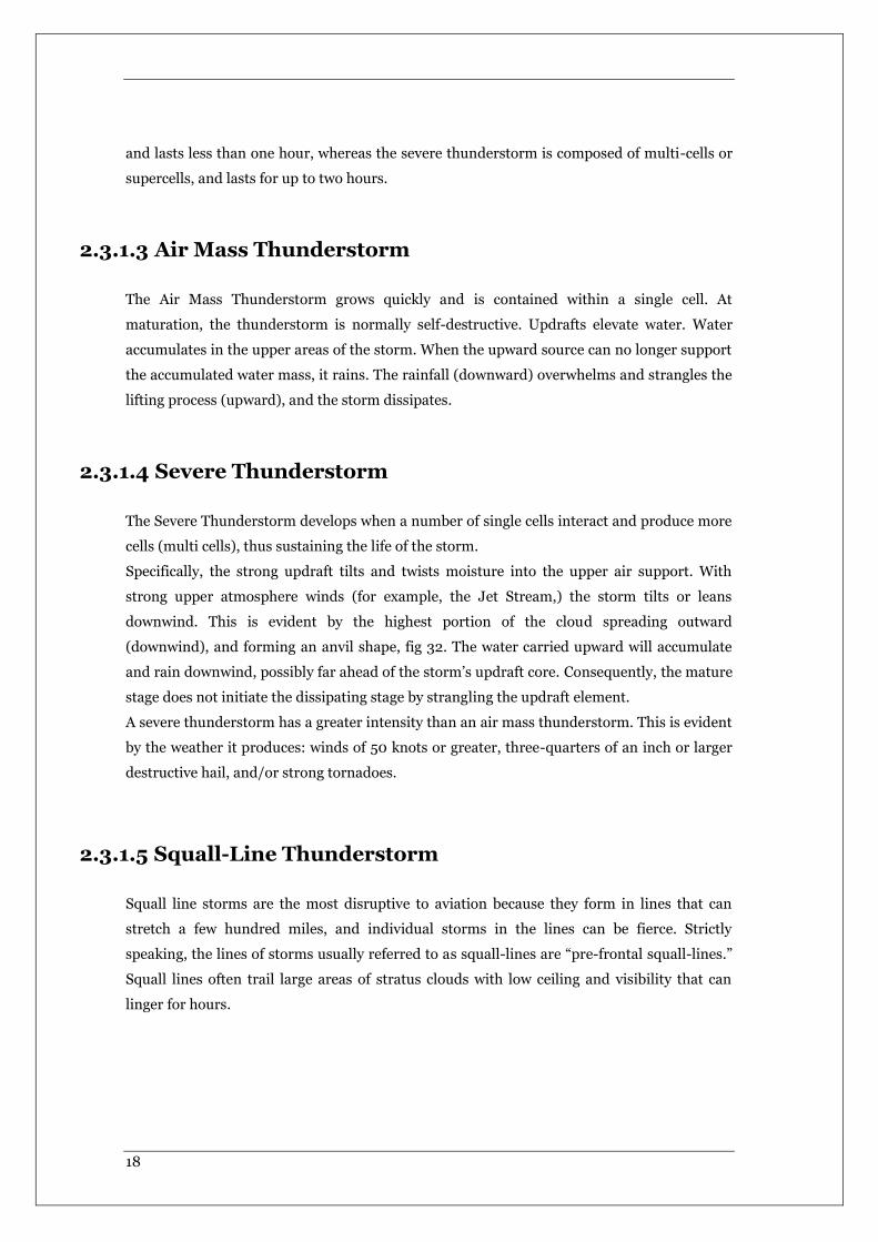
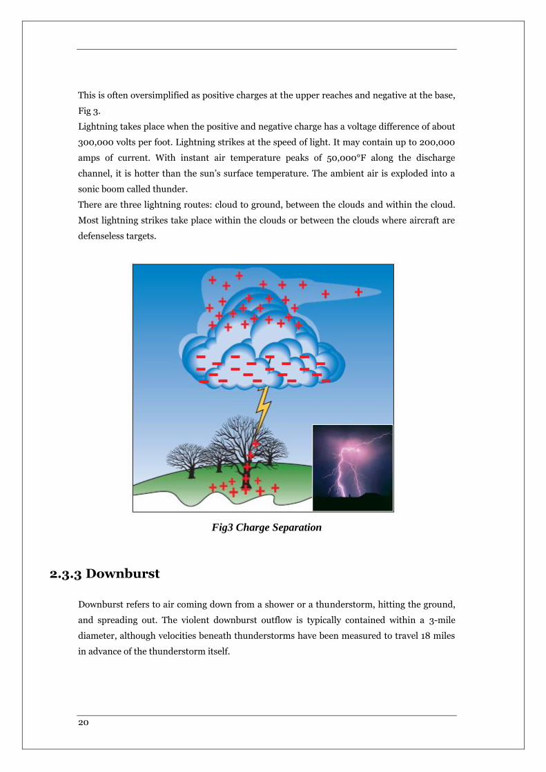
2.3.2 Lightning

Lightning is the visible electrical discharge produced by thunderstorms. The convective flow

of air currents circulating up and down create friction between the opposing air currents. The

friction causes electrical charges within the thunderstorm to separate. Charge separation in

the thunderstorm polarizes a region with positive charges at the top, intermediate negative

charges within the center, and with positive charges at the base. Since electrical opposites

attract, an invisible shadow of negative charges track along the ground beneath the

thunderstorm.

20

This is often oversimplified as positive charges at the upper reaches and negative at the base,

Fig 3.

Lightning takes place when the positive and negative charge has a voltage difference of about

300,000 volts per foot. Lightning strikes at the speed of light. It may contain up to 200,000

amps of current. With instant air temperature peaks of 50,000°F along the discharge

channel, it is hotter than the sun’s surface temperature. The ambient air is exploded into a

sonic boom called thunder.

There are three lightning routes: cloud to ground, between the clouds and within the cloud.

Most lightning strikes take place within the clouds or between the clouds where aircraft are

defenseless targets.

Fig3 Charge Separation

2.3.3 Downburst

Downburst refers to air coming down from a shower or a thunderstorm, hitting the ground,

and spreading out. The violent downburst outflow is typically contained within a 3-mile

diameter, although velocities beneath thunderstorms have been measured to travel 18 miles

in advance of the thunderstorm itself.

21

2.3.4 Wind Shear

Wind shear is the sudden “tearing” or “shearing” effect when there is a violent change of

wind over a short distance. The change can occur in either speed or direction (horizontal and

vertical), or both. Wind shear occurs when a concentrated, severe downdraft from within the

thunderstorm, known as a downburst, sends an outward burst of very strong damaging

winds toward the ground [70,71].

The effect of wind shear on an aircraft can be devastating, especially in low level flight such

as taking-off or landing. In these stages of flight the aircraft’s performance is severely

degraded beyond its capability to compensate.

Wind shear, sometimes referred to as wind shear or wind gradient, is a difference in wind

speed and/or direction over a relatively short distance in the atmosphere. Atmospheric wind

shear is normally described as either vertical or horizontal wind shear. Vertical wind shear is

a change in wind speed or direction with change in altitude. Horizontal wind shear is a

change in wind speed with change in lateral position for a given altitude. [14]

Wind shear is a microscale meteorological phenomenon occurring over a very small distance,

but it can be associated with mesoscale or synoptic scale weather features such as squall lines

and cold fronts. It is commonly observed near microbursts and downbursts caused by

thunderstorms, fronts, areas of locally higher low-level winds referred to as low level jets,

near mountains, radiation inversions that occur due to clear skies and calm winds, buildings,

wind turbines, and sailboats. Wind shear has a significant effect during take-off and landing

of aircraft due to its effects on control of the aircraft, and it has been a sole or contributing

cause of many aircraft accidents.

Wind shear is sometimes experienced by pedestrians at ground level when walking across a

plaza towards a tower block and suddenly encountering a strong wind stream that is flowing

around the base of the tower. This phenomenon is a concern for architects.

Sound movement through the atmosphere is affected by wind shear, which can bend the

wave front, causing sounds to be heard where they normally would not, or vice versa. Strong

vertical wind shear within the troposphere also inhibits tropical cyclone development, but

helps to organize individual thunderstorms into longer life cycles which can then produce

severe weather. The thermal wind concept explains how differences in wind speed at

different heights are dependent on horizontal temperature differences, and explains the

existence of the jet stream. [14,15]

22

2.3.5 Tornado

A Tornado is a swirling column of upward flowing air which is found below cumulonimbus

clouds. Wind speeds of up to 180 kts have been recorded. Tornadoes typically have a

diameter of 300 feet to 2,000 feet, although there are reported tornadoes of one mile. They

occur typically on the south to southwest side of severe thunderstorms in the mid-west. In

fact, they occur on the water side, the source of energy.

Storms spawning tornadoes must be given the widest avoidance.

2.3.6 Hail

Hail is precipitation that falls from thunderstorms as round or irregular balls of ice. The

freezing process takes place when water droplets are continuously rotated up and down by

air currents within the cell of a thunderstorm. Each time a water droplet is pushed by strong

updrafts into the cold upper layers, freezing occurs. The process repeats itself until the

weight of the hail stone causes it to fall or the updraft subsides enough to allow hail to fall to

the ground.

Hail has exited thunderstorms from the long cirrus anvil cloud, many miles distant from the

storm center. Hail paths 20 miles down-wind are common.

2.3.7 Airframe Icing

Airframe icing occurs mainly when the aircraft contacts super-cooled water droplets within

clouds. Airframe ice seriously degrades the performance and control of any airplane. All

thunderstorms contain super cooled water droplets and must be avoided.

2.4 Weather models for aeronautical applications

An atmospheric model is a mathematical model constructed around the full set of

primitive dynamical equations which govern atmospheric motions. It can supplement these

equations with parameterizations for turbulent diffusion, radiation, moist processes (clouds

and precipitation), heat exchange, soil, vegetation, surface water, the kinematic effects of

terrain, and convection. Most atmospheric models are numerical, i.e. they discretize

23

equations of motion. They can predict microscale phenomena such as tornadoes, sub-

microscale turbulent flow over buildings, as well as synoptic and global flows. The horizontal

domain of a model is either global, covering the entire Earth, or regional (limited-area),

covering only part of the Earth. The different types of models run are thermos-tropic, baro-

tropic, hydrostatic, and non-hydrostatic. Some of the model types make assumptions about

the atmosphere which lengthens the time steps used and increases computational speed.

Forecasts are computed using mathematical equations for the physics and dynamics of

the atmosphere. These equations are nonlinear and are impossible to solve exactly.

Therefore, numerical methods obtain approximate solutions. Different models use different

solution methods. Global models often use spectral methods for the horizontal dimensions

and finite-difference methods for the vertical dimension, while regional models usually use

finite-difference methods in all three dimensions. For specific locations, model output

statistics use climate information, output from numerical weather prediction, and current

surface weather observations to develop statistical relationships which account for model

bias and resolution issues.

There are several numerical weather models available, the main ones are the global

version and the regional version [17].

2.4.1 Global versions

Some of the better known global numerical models [13,14,15] are:

- GFS Global Forecast System (previously AVN) – developed by NOAA

- NOGAPS – developed by the US Navy to compare with the GFS

- GEM Global Environmental Multiscale Model – developed by the Meteorological

Service of Canada (MSC)

- IFS developed by the European Centre for Medium-Range Weather Forecasts

- UM Unified Model developed by the UK Met Office, but is hand-corrected by

professional forecasters

- GME developed by the German Weather Service, DWD, NWP Global model of DWD

- ARPEGE developed by the French Weather Service, Météo-France

- IGCM Intermediate General Circulation Model

2.4.2 Regional versions

Some of the better known regional numerical models are:

24

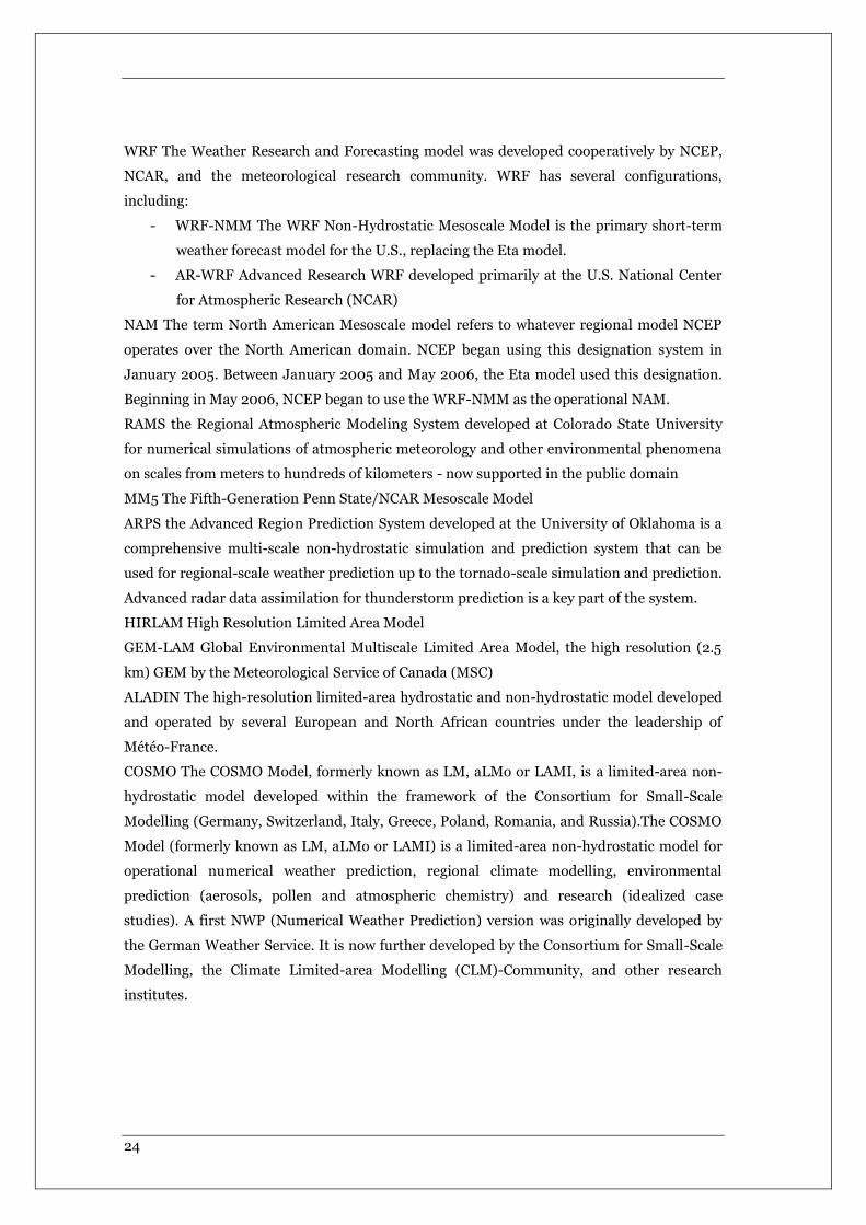
WRF The Weather Research and Forecasting model was developed cooperatively by NCEP,

NCAR, and the meteorological research community. WRF has several configurations,

including:

- WRF-NMM The WRF Non-Hydrostatic Mesoscale Model is the primary short-term

weather forecast model for the U.S., replacing the Eta model.

- AR-WRF Advanced Research WRF developed primarily at the U.S. National Center

for Atmospheric Research (NCAR)

NAM The term North American Mesoscale model refers to whatever regional model NCEP

operates over the North American domain. NCEP began using this designation system in

January 2005. Between January 2005 and May 2006, the Eta model used this designation.

Beginning in May 2006, NCEP began to use the WRF-NMM as the operational NAM.

RAMS the Regional Atmospheric Modeling System developed at Colorado State University

for numerical simulations of atmospheric meteorology and other environmental phenomena

on scales from meters to hundreds of kilometers - now supported in the public domain

MM5 The Fifth-Generation Penn State/NCAR Mesoscale Model

ARPS the Advanced Region Prediction System developed at the University of Oklahoma is a

comprehensive multi-scale non-hydrostatic simulation and prediction system that can be

used for regional-scale weather prediction up to the tornado-scale simulation and prediction.

Advanced radar data assimilation for thunderstorm prediction is a key part of the system.

HIRLAM High Resolution Limited Area Model

GEM-LAM Global Environmental Multiscale Limited Area Model, the high resolution (2.5

km) GEM by the Meteorological Service of Canada (MSC)

ALADIN The high-resolution limited-area hydrostatic and non-hydrostatic model developed

and operated by several European and North African countries under the leadership of

Météo-France.

COSMO The COSMO Model, formerly known as LM, aLMo or LAMI, is a limited-area non-

hydrostatic model developed within the framework of the Consortium for Small-Scale

Modelling (Germany, Switzerland, Italy, Greece, Poland, Romania, and Russia).The COSMO

Model (formerly known as LM, aLMo or LAMI) is a limited-area non-hydrostatic model for

operational numerical weather prediction, regional climate modelling, environmental

prediction (aerosols, pollen and atmospheric chemistry) and research (idealized case

studies). A first NWP (Numerical Weather Prediction) version was originally developed by

the German Weather Service. It is now further developed by the Consortium for Small-Scale

Modelling, the Climate Limited-area Modelling (CLM)-Community, and other research

institutes.

25

2.4.3 GRIB files

The most used meteorological file format is the GRIB (GRIdded Binary or General Regularly-

distributed Information in Binary form) from NOAA (National Oceanic and Atmospheric

Administration) [11]. The Grib is a concise data format commonly used in meteorology to

store historical and forecast weather data. The World Meteorological Organization’s

Commission for Basic Systems standardize it. Currently there are three versions of GRIB.

The first edition (current sub-version is 2) is used operationally worldwide by most

meteorological centers, for Numerical Weather Prediction output (NWP). A newer

generation has been introduced, known as GRIB second edition, and data is slowly changing

over to this format. Some of the second-generation GRIB are used for derived product

distributed in Eumetcast of Meteosat Second Generation. Another example is the NAM

(North American Mesoscale) model.

GRIB files are a collection of self-contained records of 2D data, and the individual records

stand alone as meaningful data, with no references to other records or to an overall schema.

Each GRIB record has two components - the part that describes the record (the header), and

the actual binary data itself. The data in GRIB-1 are typically converted to integers using

scale and offset, and then bit-packed. GRIB-2 also has the possibility of compression.

The most used GRIB files are the Rapid Refresh (RAP) model from NOAA/NCEP operational

weather prediction system, running every hour. Such a file contains all the atmospheric

conditions required to predict aircraft consumption and emissions.

The RAP is an atmospheric prediction system that consists primarily of a numerical forecast

model and an analysis system to initialize the model. Models run hourly, with analysis and

hourly forecasts out to 18 hours. RAP files are stored in the GRIB2 file format. The minimum

grid spatial resolution is 13 km. In particular, for the tests were used GRIB2 file that uses 37

vertical levels (isobaric levels) with a grid having a horizontal spatial resolution of 20 km

with a dimension of 225x301 grid cells. From these files were used geo-referred information

about pressure, temperature, relative humidity, wind speed and direction, and clouds

reflectivity (from on-ground the weather radar data), the other variable needed were taken

from ISA standard model.

2.5 Devices used to detect weather phenomenon

For a pilot situational awareness, the primary source of information about the weather

conditions like wind, perturbation, pressure, temperature, humidity, etc. They can be

detected on board or on ground with different devices [12,16] that will be described in the

following paragraphs.

26

2.5.1 Onboard information sources

Service aircraft integrate a few number of sensors, commonly used for navigation

purposes and to provide environment information to the pilot. The Air Data and Inertial

Reference System (ADIRS) calculates flight parameters (Indicated Airspeed, position, etc)

directly from probe measurements and supplies with air data a large number of critical

aircraft systems (like FMS). The probes network, used for navigation, includes the following

sensors:

- Pressure sensors (Pitot probes, Pitot-static probes and static pressure probes)

- Temperature sensors (total air temperature probes)

- Angle of Attack sensors

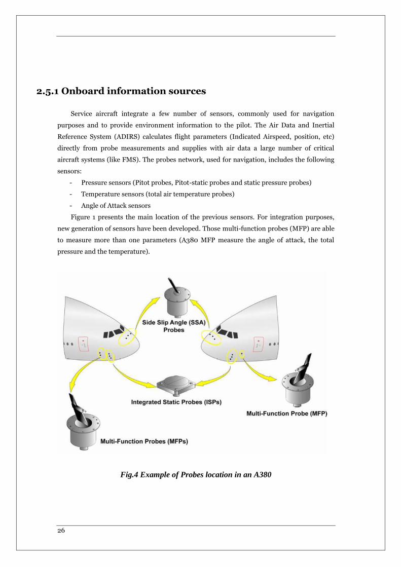
Figure 1 presents the main location of the previous sensors. For integration purposes,

new generation of sensors have been developed. Those multi-function probes (MFP) are able

to measure more than one parameters (A380 MFP measure the angle of attack, the total

pressure and the temperature).

Fig.4 Example of Probes location in an A380

27

2.5.1.1 Pressure

Pressure sensors measure various type of pressures, depending on their position and type:

- The static pressure sensor, which measures the static pressure

- The Pitot sensor, which measure the total pressure

- The Pitot-static sensor, which measure both static and total pressure

The statics pressure sensor is used to determine the statics pressure. This information is

crucial since, combined with Pitot sensors measurements, it is used to calculates the aircraft

velocity (the Indicated Air Speed, which leads to the True Air Speed) and wind speed

(combined with inertial data). The number of integrated static pressure sensors varies by

manufacturer and aircraft model. Airbus commercial aircrafts are commonly equipped with

6 pressure sensors (3 on each side of the aircraft) while Boeing usually use 3 probes per

aircraft. The Pitot sensor provides the aircraft with the total pressure (sum of dynamic

pressure and static pressure). The probe is an opened trend tube, parallel with the air flow.

The delta between total pressure and static pressure provides the dynamic pressure, required

to determine the relative wind speed and the Mach number.

2.5.1.2 Temperature

The total air temperature probes sense total air temperature (TAT), used to calculate the

static air temperature (SAT or outer air temperature OAT). The TAT (see Fig. 4) is directly

sent to the ADIRS and used (with static and total pressure) to compute the true air speed

(TAS). The information is also displayed to the pilot on the electronic flight instrument

system (EFIS).

The temperature sensors tolerance is ± 0.25°C plus 0.5% percent of the magnitude of the

temperature in degrees Celsius, with a response time in the air around 1 second.

2.5.1.3 Multi-function probe

The Multi-Function Probe (MFP) combines two or more sensors. This type of probes does

not provide any new weather parameter to the aircraft but reduce the number of probes

integrated in the fuselage for cost efficiency, and drag reducing purposes. The MFP does not

refer to a clear need, and each aircraft and manufacturer integrate different functionalities to

the sensor, depending on the aircraft need. The MFP integrated in the A380 and A350

(provided by Goodrich) supply total pressure, total air temperature and angle of attack data

(Fig. 5). The static pressure is measure by dedicated probes located on each side of the

28

aircraft. For redundancy purposes, temperature sensors have also been added in the A350

fuselage.

Fig.5 Example of A380 Multi-Function Probes

2.5.1.4 Humidity

Humidity sensors offer real opportunities to improve weather forecast on specific

phenomena (clear air turbulence, icing, convection) and provide in-situ measures to evaluate

climate changes. Only few aircrafts are already equipped with humidity sensors in Europe

but WMO initiative E-AMDAR promotes the integration of hygrometric sensors to improve

weather forecast. There are few humidity sensors integrated in European commercial

aviation yet but offer a real interest to improve weather forecast. This section will first specify

the needs in term of performance and then detail two available humidity sensors integrated

in American commercial aviation for AMDAR operating system.

2.5.1.5 Onboard Weather radar

Weather radar is designed to detect precipitation: it helps to identify that associated with the

most active convective cells in order to avoid the dangers associated with them (turbulence,

hail and lightning).

Weather radar can detect water in liquid form, such as rain and wet hail. However, it hardly

detects water in solid form such as dry snow and ice crystals. It can partly detect dry hail

depending on the size of the hailstones.

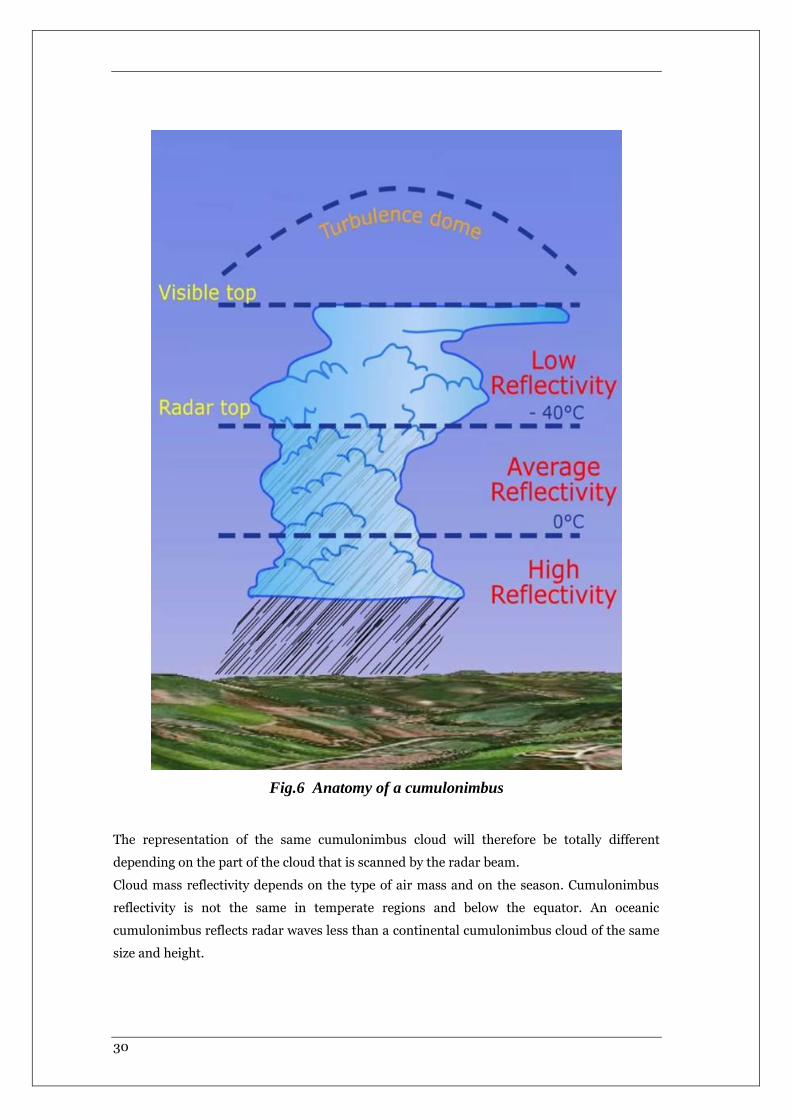
In a convective cell, in the part situated below freezing point (0 °C, that mean FL 75 in

standard atmosphere), liquid precipitation constitutes the most reflective areas. Below -40°C

(at FL 275 in standard atmosphere) water no longer exists in general in a liquid state. In the

part of the cumulonimbus between freezing point and the altitude where the temperature

29

reaches -40 °C, liquid water and ice crystals produce areas where reflectivity decreases

depending on the variation of the presence of liquid water. In the part above the altitude

where the temperature reaches -40 °C, where there are only ice crystals, reflectivity is very

low.

Areas returning most of the radar signal may be harmless for flight, like melted snow

showers for example, whereas hail showers which constitute a genuine threat to navigation

may only return a weak radar echo.

When cumulonimbus clouds swell swiftly, they may be overtaken by a zone of severe

turbulence which could stretch several thousand feet above the visible peak. This turbulence

zone is invisible to weather radar and the naked eye (The TURB function, which uses the

principle of the Doppler effect, only helps detection of turbulence in wet zones).

30

Fig.6 Anatomy of a cumulonimbus

The representation of the same cumulonimbus cloud will therefore be totally different

depending on the part of the cloud that is scanned by the radar beam.

Cloud mass reflectivity depends on the type of air mass and on the season. Cumulonimbus

reflectivity is not the same in temperate regions and below the equator. An oceanic

cumulonimbus reflects radar waves less than a continental cumulonimbus cloud of the same

size and height.

31

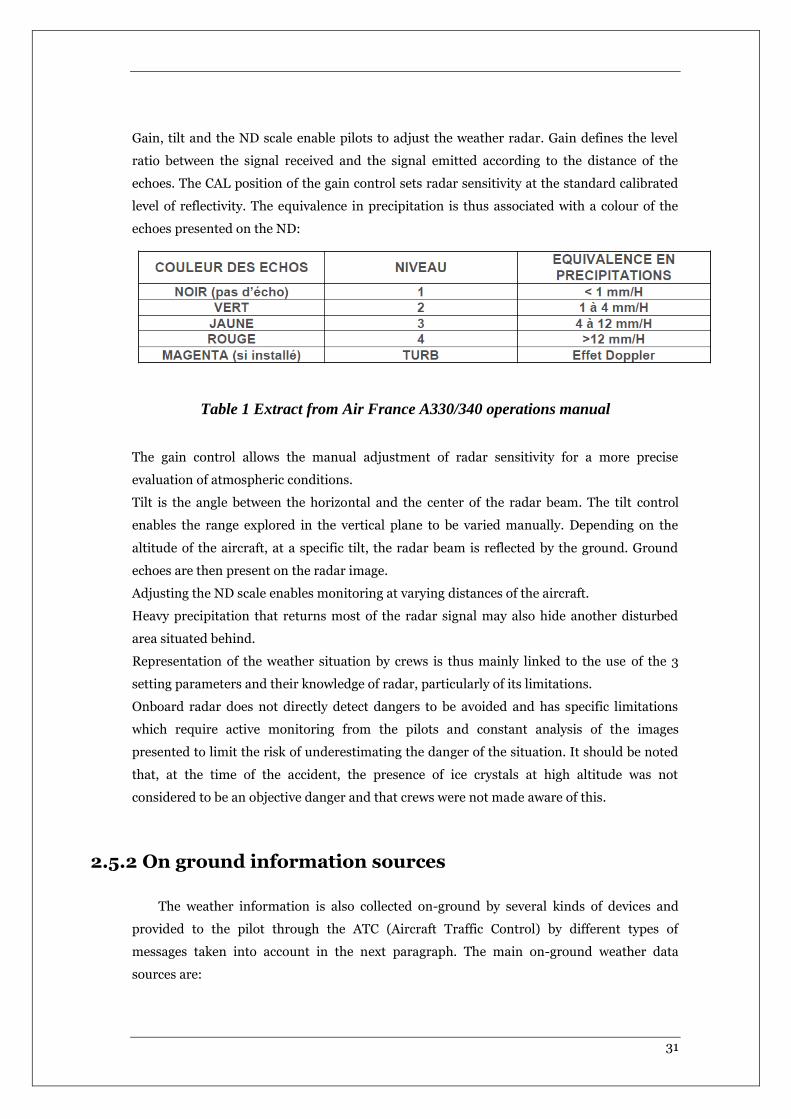
Gain, tilt and the ND scale enable pilots to adjust the weather radar. Gain defines the level

ratio between the signal received and the signal emitted according to the distance of the

echoes. The CAL position of the gain control sets radar sensitivity at the standard calibrated

level of reflectivity. The equivalence in precipitation is thus associated with a colour of the

echoes presented on the ND:

Table 1 Extract from Air France A330/340 operations manual

The gain control allows the manual adjustment of radar sensitivity for a more precise

evaluation of atmospheric conditions.

Tilt is the angle between the horizontal and the center of the radar beam. The tilt control

enables the range explored in the vertical plane to be varied manually. Depending on the

altitude of the aircraft, at a specific tilt, the radar beam is reflected by the ground. Ground

echoes are then present on the radar image.

Adjusting the ND scale enables monitoring at varying distances of the aircraft.

Heavy precipitation that returns most of the radar signal may also hide another disturbed

area situated behind.

Representation of the weather situation by crews is thus mainly linked to the use of the 3

setting parameters and their knowledge of radar, particularly of its limitations.

Onboard radar does not directly detect dangers to be avoided and has specific limitations

which require active monitoring from the pilots and constant analysis of the images

presented to limit the risk of underestimating the danger of the situation. It should be noted

that, at the time of the accident, the presence of ice crystals at high altitude was not

considered to be an objective danger and that crews were not made aware of this.

2.5.2 On ground information sources

The weather information is also collected on-ground by several kinds of devices and

provided to the pilot through the ATC (Aircraft Traffic Control) by different types of

messages taken into account in the next paragraph. The main on-ground weather data

sources are:

32

- On-ground weather radar

- Meteorological stations

- On-ground meteorological predictions

The on-ground weather radar has the same behavior of the on-board weather data, the

meteorological stations are composed by different sensors, similar to the on-board sensors.

The meteorological predictions are based on the meteorological models described in the

previous paragraphs.

33

CHAPTER 3

OVERVIEW ON CIVIL

AIRCRAFT FLIGHT

Aircraft can be divided in 3 main weight categories that have a different behavior respect the

weather condition and trajectory. In this chapter are described and characterized the 3

aircraft categories, the phase of flight in which the aircraft trajectory can be divided and an

overview of the trajectory optimization methods is provided.

3.1 Aircraft categories

The ICAO wake turbulence category (WTC) is entered in the appropriate single character

wake turbulence category indicator in Item 9 of the ICAO model flight plan form and is based

on the maximum certificated take-off mass, as follows [13]:

- H (Heavy) aircraft types of 136 000 kg (300 000 lb) or more (i.e. long range aircraft

like A320);

- M (Medium) aircraft types less than 136 000 kg (300 000 lb) and more than 7 000

kg (15 500 lb) (i.e. regional aircraft like ATR72); and

- L (Light) aircraft types of 7 000 kg (15 500 lb) or less (i.e. ultra-light aircraft like

Cessna)

34

Variants of an aircraft type may fall into different wake turbulence categories, (e.g. L/M or

M/H). In these cases, it is the responsibility of the pilot or operator to enter the appropriate

wake turbulence category indicator in the flight plan.

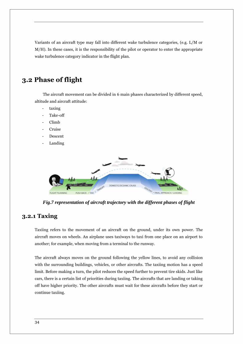
3.2 Phase of flight

The aircraft movement can be divided in 6 main phases characterized by different speed,

altitude and aircraft attitude:

- taxing

- Take-off

- Climb

- Cruise

- Descent

- Landing

Fig.7 representation of aircraft trajectory with the different phases of flight

3.2.1 Taxing

Taxiing refers to the movement of an aircraft on the ground, under its own power. The

aircraft moves on wheels. An airplane uses taxiways to taxi from one place on an airport to

another; for example, when moving from a terminal to the runway.

The aircraft always moves on the ground following the yellow lines, to avoid any collision

with the surrounding buildings, vehicles, or other aircrafts. The taxiing motion has a speed

limit. Before making a turn, the pilot reduces the speed further to prevent tire skids. Just like

cars, there is a certain list of priorities during taxiing. The aircrafts that are landing or taking

off have higher priority. The other aircrafts must wait for these aircrafts before they start or

continue taxiing.

35

The thrust to propel the aircraft forward comes from its propellers or jet engines. Steering is

achieved by turning a nose wheel or tail wheel/rudder; the pilot controlling the direction

travelled with their feet. The use of engine thrust near terminals is restricted due to the

possibility of jet blast damage. Therefore, the aircrafts are pushed back from the buildings by

a vehicle before they can start their own engines for taxiing.

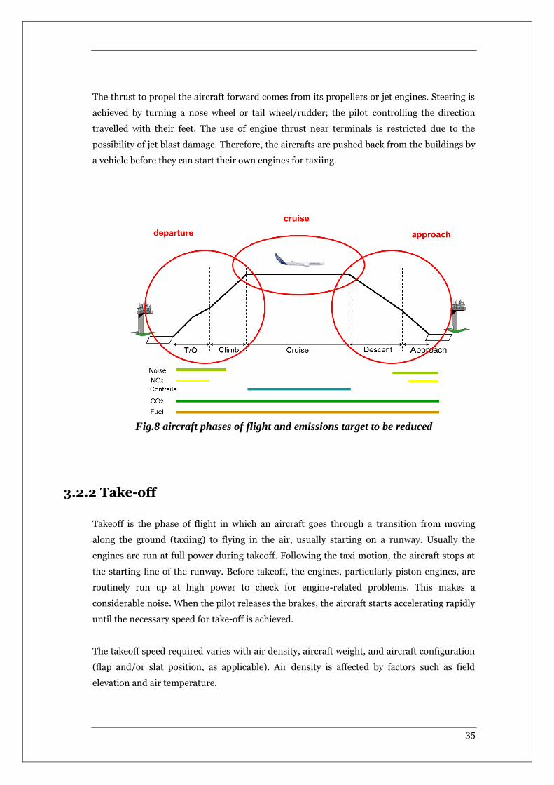
Fig.8 aircraft phases of flight and emissions target to be reduced

3.2.2 Take-off

Takeoff is the phase of flight in which an aircraft goes through a transition from moving

along the ground (taxiing) to flying in the air, usually starting on a runway. Usually the

engines are run at full power during takeoff. Following the taxi motion, the aircraft stops at

the starting line of the runway. Before takeoff, the engines, particularly piston engines, are

routinely run up at high power to check for engine-related problems. This makes a

considerable noise. When the pilot releases the brakes, the aircraft starts accelerating rapidly

until the necessary speed for take-off is achieved.

The takeoff speed required varies with air density, aircraft weight, and aircraft configuration

(flap and/or slat position, as applicable). Air density is affected by factors such as field

elevation and air temperature.

36

The speeds needed for takeoff are relative to the motion of the air (indicated airspeed). A

head wind will reduce the ground speed needed for takeoff, as there is a greater flow of air

over the wings. This is why the aircraft generally take off against the wind. Side wind is not

preferred as it would disturb the stability of the aircraft. Typical takeoff air speeds for

jetliners are in the 130–155 knot range (150–180 mph, 240–285 km/h). For a given aircraft,

the takeoff speed is usually directly proportional to the aircraft weight; the heavier the

weight, the greater the speed needed. Some aircraft have difficulty generating enough lift at

the low speeds encountered during takeoff. These are therefore fitted with high lift devices,

often including slats and usually flaps, which increase the camber of the wing, making it

more effective at low speed, thus creating more lift. These have to be deployed from the wing

before performing any maneuver.

At the beginning of the climb phase, the wheels are retracted into the aircraft and the

undercarriage doors are closed. This operation is audible by the passengers as a noise coming

from below the floor.

3.2.3 Climb

Following take-off, the aircraft has to climb to a certain altitude (typically 30,000 ft or 10

km) before it can cruise at this altitude in a safe and economic way. A climb is carried out by

increasing the lift of wings supporting the aircraft until their lifting force exceeds the weight

of the aircraft. Once this occurs, the aircraft will climb to a higher altitude until the lifting

force and weight are again in balance. The increase in lift may be accomplished by increasing

the angle of attack of the wings, by increasing the thrust of the engines to increase speed

(thereby increasing lift), by increasing the surface area or shape of the wing to produce

greater lift, or by some combination of these techniques. In most cases, engine thrust and

angle of attack are simultaneously increased to produce a climb.

Because lift diminishes with decreasing air density, a climb, once initiated, will end by itself

when the diminishing lift with increasing altitude drops to a point that equals the weight of

the aircraft. At that point, the aircraft will return to level flight at a constant altitude. During

climb phase, it is normal that the engine noise diminishes. This is because the engines are

operated at a lower power level after the take-off. It is also possible to hear a whirring noise

or a change in the tone of the noise during climb. This is the sound of the flaps that are

retracting. A wing with retracted flap produces less noise.

37

3.2.4 Cruise

Cruise is the level portion of aircraft travel where flight is most fuel efficient. It occurs

between ascent and descent phases and is usually the majority of a journey. Technically,

cruising consists in a flight with constant airspeed and altitude. It ends as the aircraft

approaches the destination where the descent phase of flight commences in preparation for

landing.

For most commercial passenger aircraft, the cruise phase of flight consumes the majority of

fuel. As this lightens the aircraft considerably, higher altitudes are more efficient for

additional fuel economy. However, for operational and air traffic control reasons it is

necessary to stay at the cleared flight level. Typical cruising speed for long-distance

commercial passenger flights is 475-500 knots (878-926 km/h; 547-578 mph).

Commercial or passenger aircraft are usually designed for optimum performance at their

cruise speed. There is also an optimum cruise altitude for a particular aircraft type and

conditions including payload weight, center of gravity, air temperature, humidity, and speed.

This altitude is usually where the drag is minimum and the lift is maximum. As in any phase

of the flight, the aircraft in cruise mode is always in communication with an Air Traffic

Control (ATC) station. Although the general tendency is to follow a straight line towards the

destination, there may be some deviations from the flight plan for weather, turbulence or air

traffic rea- sons, after receiving clearance from ATC.

3.2.5 Descent

A descent during air travel is any portion where an aircraft decreases altitude. Descents are

an essential component of an approach to landing. Other partial descents might be to avoid

traffic, poor flight conditions (turbulence or bad weather), clouds (particularly under visual

flight rules), to see something lower, to enter warmer air (in the case of extreme cold), or to

take advantage of wind direction of a different altitude. Normal descents take place at a

constant airspeed and constant angle of descent (3-degree final approach at most airports).

The pilot controls the angle of descent by varying engine power and pitch angle (lowering the

nose) to keep the airspeed constant.

A peculiar flight technique is applied from Pilot to save fuel and obtain noise abatement

during descent. This technique is based on a computation of the “top of descent point”, a

38

point where, if no diversion (traffic or weather) occurs, engines power will be reduced and

never increase till landing phase. In other words, the achievement is a continue descent to

the destination airport whiteout any interruption of level flight phase such required an

increase of engine power, fuel consumption and noise.

At the beginning of and during the descent phase, the engine noise diminishes further as the

engines are operated at low power settings. However, towards the end of the descent phase,

the passenger can feel further accelerations and an increase in the noise. This is to realize the

“final approach” before taking “landing position”.

3.2.6 Landing

Landing is the last part of a flight, where the aircraft returns to the ground. Aircraft usually

land at an airport on a firm runway, generally constructed of asphalt concrete, concrete,

gravel or grass. To land, the airspeed and the rate of descent are reduced to where the object

descends at a slow enough rate to allow for a gentle touch down. Landing is accomplished by

slowing down and descending to the runway. This speed reduction is accomplished by

reducing thrust and/or inducing a greater amount of drag using flaps, landing gear or speed

brakes. As the plane approaches the ground, the pilot will execute a flare (round out) to

induce a gentle landing. Although the pilots are trained to perform the landing operation,

there are “Instrument Landing Systems” in most of the airports to help pilots land the

aircraft. An instrument landing system (ILS) is a ground-based instrument approach system

that provides precision guidance to an aircraft approaching and landing on a runway, using a

combination of radio signals and, in many cases, high-intensity lighting arrays to enable a

safe landing during instrument meteorological conditions (IMC), such as low ceilings or

reduced visibility due to fog, rain, or blowing snow.

At the beginning of the landing phase, the passengers will hear the opening of the doors of

the landing gears. As the landing gears are deployed, they will create an additional drag and

an additional noise. Immediately after touch-down, the passengers can hear a blowing

sound, sometimes with increasing engine sound. This is the engine’s thrust reverses, helping

the aircraft to slow down to taxi speeds by redirecting the airflow of the engines for- ward. Is

a way to decelerate without overload the landing gear braking system. This phase is the

noisiest of landing. Once the aircraft is decelerated to low speed, it can taxi to the terminal

building.

39

3.3 Flight Planning

The process of producing a flight plan to describe the trajectory of a proposed flight is called

flight planning. It basically involves coming with an estimate of amount of fuel required for

the flight and the trajectory of flight, describing the route to be taken to reach the destination

safely, which complies with the air traffic control procedures/regulations. Civil airlines would

wish to plan the trajectory in such a way that it would minimize a certain cost index.

The procedure of coming up with a flight plan is highly dependent on a lot of factors and is

very problem specific. It depends on specific origin-destination pair, type of aircraft being

used and weather forecast. Flight planning requires accurate weather forecasts so that fuel

consumption calculations can account for the fuel consumption effects of head or tail winds

and air temperature. Producing an optimal flight plan even for a given origin-destination

pair, a specific aircraft and initial weight, is never a one-time process. The air temperature

aspects the efficiency/fuel consumption of

aircraft engines. The wind may provide a head or tail wind component which in turn will

increase or decrease the fuel consumption by increasing or decreasing the air distance to be

own. Hence, accurately updated weather forecast plays a crucial role in coming up with an

optimal trajectory.

Furthermore, it is required as per safety procedures to carry fuel beyond the minimum

needed to y to the specified destination. Under the supervision of air traffic control, aircraft

flying in controlled airspace must follow predetermined routes known as airways, even if

such routes are not as economical as a more direct flight.

Within these airways, aircraft must maintain flight levels, specified altitudes usually

separated vertically by 1000 or 2000 feet, depending on the route being own and the

direction of travel. When aircraft with only two engines are flying long distances across

oceans, deserts, or other areas with no airports, they have to satisfy extra safety rules to

ensure that such aircraft can reach some emergency airport if one engine fails. Rate of fuel

burn depends on ambient temperature, aircraft speed, and aircraft altitude, none of which

are entirely predictable. Rate of fuel burn also depends on airplane weight, which changes as

fuel is burned.

Coming up with an accurate optimized flight plan for commercial airlines is by itself a big

industry. Producing an accurate optimized flight plan requires a large number of calculations

(millions), so commercial flight planning systems make extensive use of computers. Some

commercial airlines have their own internal flight planning system, while others employ the

services of external planners. While developing a software tool to plan flight trajectory, it is

necessary to incorporate commercial flight procedures followed. They add in a lot more

constraints to the flight path. These are discussed in the following section.

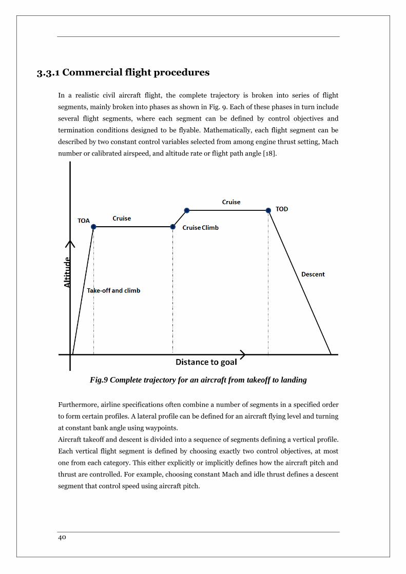
40

3.3.1 Commercial flight procedures

In a realistic civil aircraft flight, the complete trajectory is broken into series of flight

segments, mainly broken into phases as shown in Fig. 9. Each of these phases in turn include

several flight segments, where each segment can be defined by control objectives and

termination conditions designed to be flyable. Mathematically, each flight segment can be

described by two constant control variables selected from among engine thrust setting, Mach

number or calibrated airspeed, and altitude rate or flight path angle [18].

Fig.9 Complete trajectory for an aircraft from takeoff to landing

Furthermore, airline specifications often combine a number of segments in a specified order

to form certain profiles. A lateral profile can be defined for an aircraft flying level and turning

at constant bank angle using waypoints.

Aircraft takeoff and descent is divided into a sequence of segments defining a vertical profile.

Each vertical flight segment is defined by choosing exactly two control objectives, at most

one from each category. This either explicitly or implicitly defines how the aircraft pitch and

thrust are controlled. For example, choosing constant Mach and idle thrust defines a descent

segment that control speed using aircraft pitch.

41

3.3.1.1 Lateral profile

Lateral profile of a flight usually describes the level flight portion. The aircraft makes turns at

a constant bank angle. A lateral profile is usually described by a sequence of waypoints (Area

Navigation (RNAV)). Most waypoints are classified as compulsory reporting points, i.e. the

pilot (or the onboard flight management system) reports the aircraft position to air traffic

control as the aircraft passes a waypoint. There are two main types of waypoints. A named

waypoint appears on aviation charts with a known latitude and longitude. Such waypoints

over land often have an associated radio beacon so that pilots can more easily check where

they are. Useful named waypoints are always on one or more airways. A geographic waypoint

is a temporary position used in a flight plan, usually in an area where there are no named

waypoints, e.g. most oceans in the southern hemisphere. Air traffic control require that

geographic waypoints have latitudes and longitudes which are a whole number of degrees.

3.3.1.2 Vertical profile - SID & STAR

After take-off, an aircraft follows a Departure Procedure (SID or Standard Instrument

Departure) which defines a pathway from an airport runway to a waypoint on an airway, so

that an aircraft can join the airway system in a controlled manner. Most of the climb portion

of a flight will take place on the SID. Although a SID will keep aircraft away from terrain, it is

optimized for ATC route of flight and will not always provide the lowest climb gradient. It

strikes a balance between terrain and obstacle avoidance, noise abatement (if necessary) and

airspace management considerations. Before landing an aircraft follows an Arrival Procedure

(STAR or Standard Terminal Arrival Route) which defines a pathway from a waypoint on an

airway to an

airport runway, so that aircraft can leave the airway system in a controlled manner.

STAR usually covers the phase of a flight that lies between the top of descent from cruise or

en-route flight and the final approach to a runway for landing. Normally that final approach

starts at the so-called Initial Approach Fix (IAF). A typical STAR consists of a set of starting

points, called transitions, and a description of routes (typically via waypoints) from each of

these transitions to a point close to destination airport.

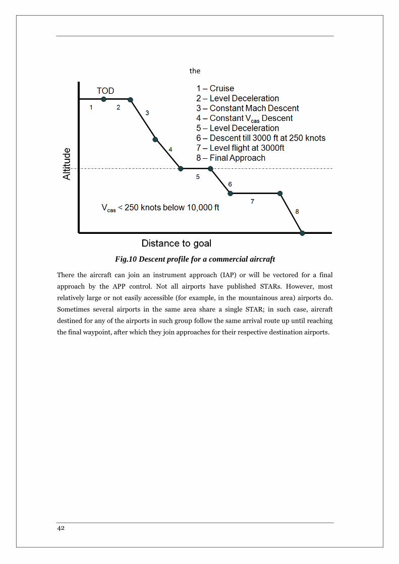
42

the

Fig.10 Descent profile for a commercial aircraft There the aircraft can join an instrument approach (IAP) or will be vectored for a final

approach by the APP control. Not all airports have published STARs. However, most

relatively large or not easily accessible (for example, in the mountainous area) airports do.

Sometimes several airports in the same area share a single STAR; in such case, aircraft

destined for any of the airports in such group follow the same arrival route up until reaching

the final waypoint, after which they join approaches for their respective destination airports.

43

CHAPTER 4

OVERVIEW ON

ALGORITHMS FOR

TRAJECTORY

OPTIMIZATION

4.1 Review of the Literature

Proposed in 1931, the Zermelo's Navigation Problem was the first posed optimal control

problem posed [33]. The problem was to find an optimal path for a boat navigating in a water

body in presence of water currents and wind. Without considering any current or wind or

any such external force, the optimal control is to follow a straight-line segment from origin to

destination. But otherwise, the optimal path is in general never the line joining origin and

destination. The same problem was formulated for an aircraft and calculus of variation

approach was used to solve it assuming a at earth. Bryson and Ho. later developed a solution

technique called neighboring optimal control (NOC) to come up with a solution for Zermelo's

problem [34]. The technique of neighboring optimal control (NOC) produces time-varying

feedback control that minimizes a performance index to second order for perturbations from

a nominal optimal path. This technique was later extended to handle cases of parameter

change in the system dynamic model [35]. This extension is used to develop an algorithm for

optimizing horizontal aircraft trajectories in general wind fields using time-varying linear

feedback gains. The minimum-time problem for an airplane traveling horizontally between

two points in a variable wind field (a type of Zermelo problem) was used to illustrate the

44

above technique. The NOC solution was derived analytically for the case where the wind field

was modeled as a constant wind Jardin and Bryson further extended the neighboring optimal

control (NOC) technique for computing minimum-time paths through general wind fields by

modeling winds along a nominally straight-line path as additional system states [36]. This

advancement, referred to as Neighboring Optimal Wind Routing (NOWR), allowed the

neighboring optimal control gain solution to be parameterized for different wind conditions

and different origin/destination pairs. The winds were modeled at an arbitrary number of

discrete points along the nominal great-circle route so that gains are computed for the wind

perturbations at each point. Gains are computed once offline and then applied to a wide

variety of trajectories between different locations at different altitudes and at different flight

speeds. Jardin further demonstrated how to apply the solution to flights on the sphere

through coordinate rotations and normalizations and presented analytical solutions for the

neighboring optimal gains. In 2010, Jardin and Bryson described two methods to solve a

minimum time flight path at high altitude in presence of strong horizontal winds [37]. The

first method was using nonlinear feedback (dynamic programming) solutions for minimum-

time flight paths. A Zermelo Problem for arbitrary winds was extended from a at earth model

to a spherical earth model as a two-state problem (latitude and longitude) with one control

(heading angle). The second method is based on an analytical neighboring optimal control

solution that computes neighboring optimal heading commands as a function of the winds

along a nominal flight path.

Most of the work mentioned above deals with the cruise portion of the flight.

Some of them even assume constant speed throughout the flight. The cruise flight being the

major portion of a flight, this has indeed been research topic with most of the works done in

flight trajectory optimization, beginning with a series of thesiss by Zagalsky et al.,[38]

Schultz and Zagalsky [39], Speyer [40] and [41], and Schultz [42].

In Ref. [38] the authors examined the long-range optimal aircraft cruise problem with the

energy-range model. Speyer in 1976 [41] proved using second-order variational analysis and

a frequency-domain version of the classical Jacobi (conjugate point) optimality condition

that the steady-state cruise for a long-time span is non-optimal with respect to fuel economy.

In 1989 P.K. Menon [43] analyzed the long-range cruise problem using point mass and an

energy model and showed that the steady state cruise exists as central member along with

several other oscillatory extremals. There has been a constant mention in the literature about

fuel efficiency of periodic flights - [44], [45] and [46].

Although not as significant as the cruise portion, the climb and the descent portion of the

flight has also been studied and optimal strategies were proposed. In 1975, A. Chakravarty in

1983 introduced the concept of an optimal cruise descent [47]. Optimal results were

compared with the conventional strategies of constant Mach, Vcas and flight path angle

descent segments. The effects of wind on cost of delay was also discussed. In [48],

45

representative minimum-fuel flight paths of various types are computed for a commercial jet

transport close to the terminal area. [49] studies the characteristics of optimum fixed-range

trajectories whose structure is constrained to climb, steady cruise, and descent segments by

using optimal control theory.

In 2002, Clarke et al. designed and flight-tested a Continuous Descent Approach (CDA or

also known as OPD - optimized descent approach) procedure for UPS operated Boeing B767-

300 aircraft at the end of the nightly UPS arrival bank at Louisville International Airport

[23]. This was mainly designed as a noise abatement procedure and it was shown to reduce

the A-weighted peak noise level at seven locations along the flight path by 3.9 to 6.5 dBA. The

CDA procedure was also shown to reduce the flight time in the terminal area of the Boeing

B767-300 aircraft used in the test by up to 100 seconds relative to the nominal approach

procedure, and the corresponding fuel burn by up to 500 pounds [50]. However, widespread

implementation of CDA has been limited by the capabilities of both air traffic controllers and

air traffic control (ATC) automation. Because it is difficult to predict the future position of an

aircraft when its speed varies significantly, air traffic controllers typically instruct all aircraft

to y a staged approach, where at each stage the aircraft maintain a common altitude and

speed. A lot of variations of CDA have also been studied. A tailored arrival was designed to

accommodate CDA under constrained airspace [51]. A tailored arrival creates a four-

dimensional continuous descent from cruise altitude to the runway. Demonstrations of

oceanic arrivals at San Francisco (SFO) have successfully demonstrated significant fuel

savings. Since 2002, significant

research has gone into studying practical implementations of CDA, its variations and

comparisons with current procedures and its efficiency - [52], [53], [54], [55], [56] and [57].

Most trajectory optimization schemes use calculus of variation or optimal control theory

which are continuous time methods. Discrete methods were also used as early as 1950's.

Dixon Speas formed a small company to serve clients in the airline industry. One of his

services was to plan minimum-time paths for flights over the Atlantic Ocean. His engineers

used discrete dynamic programming, dividing the path into 15 to 20 regions and using high

altitude wind data from weather balloons. In the 1970s, Lou Reinkins at Lockheed started a

flight planning service for airlines and private aircraft for flights in the United States.

Starting in the 1980s, Jeppesen JetPlan did

the same thing for the airlines and private pilots and included international flights.

Due to large runtime and memory management issues, discrete search strategies have

seldom been used to plan aircraft trajectories. Discrete algorithms have mainly been used in

robotics and UAV path planning in presence of obstacles. In [58], Sellier discusses the use of

discrete search methods for real time flight path optimization. It also presents discrepancies

and inefficiencies of the cost index concept which is still currently in use in the most

advanced flight management systems. Mixed integer linear programs have also been used to

46

solve for real time trajectory planning for UAV's [59] and for trajectory planning with

collision avoidance [60]. Iris Yang and Yiyuan in [61] present a discrete search strategy

potential real-time generations of four-dimensional trajectories for a single autonomous

aerospace vehicle amid known obstacles and conflicts.

There are surplus examples to show the popularity of use of discrete methods like Dijkstra's

algorithm or dynamic programming in the context of UAV's. But they have rarely been used

to plan commercial aircraft trajectories. In this work, we plan to show the effectiveness and

flexibility of A* algorithm in incorporating the large number of trajectory constraints placed

on a commercial aircraft by the air traffic regulations.

4.2 Algorithms for trajectory optimization

Trajectory optimization is the process of designing a trajectory that minimizes (or

maximizes) some measure of performance while satisfying a set of constraints. Generally

speaking, trajectory optimization is a technique for computing an open-loop solution to an

optimal control problem. It is often used for systems where computing the full closed-loop

solution is either impossible or impractical.

Although the idea of trajectory optimization has been around for hundreds of years (calculus

of variations, brachystochrone problem), it only became practical for real-world problems

with the advent of the computer. Many of the original applications of trajectory optimization

were in the aerospace industry, computing rocket and missile launch trajectories. More

recently, trajectory optimization has also been used in a wide variety of industrial process

and robotics applications.

The main typologies of optimization algorithms that we can identify are:

- Direct methods

- Indirect methods

- Shooting methods

- Collocation methods

- Mesh

In the following paragraphs, we will provide a description of a set of these algorithms.

4.2.1 The typical terminology for trajectory optimization

For sake of simplicity here are reported some definitions, related to the algorithms, that will

be used later.

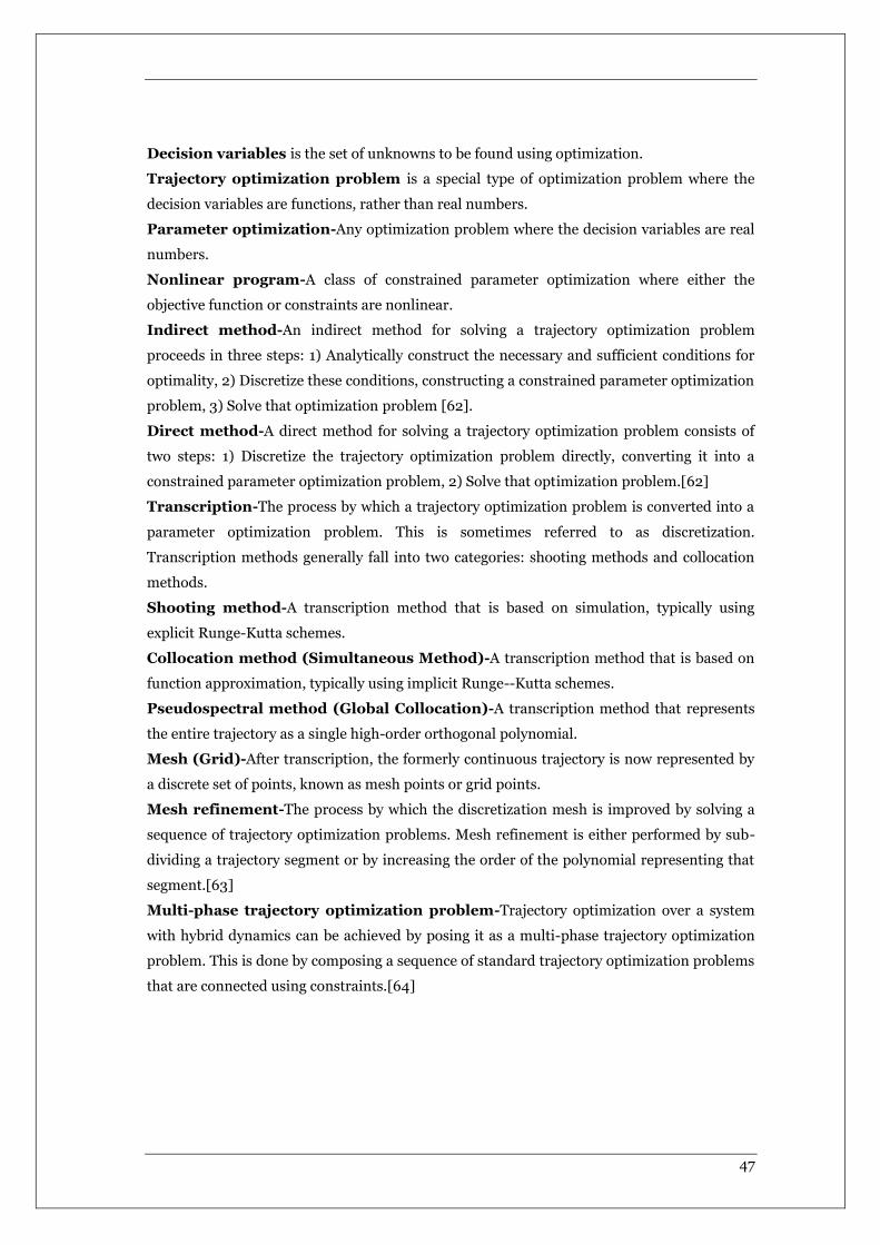
47

Decision variables is the set of unknowns to be found using optimization.

Trajectory optimization problem is a special type of optimization problem where the

decision variables are functions, rather than real numbers.

Parameter optimization-Any optimization problem where the decision variables are real

numbers.

Nonlinear program-A class of constrained parameter optimization where either the

objective function or constraints are nonlinear.

Indirect method-An indirect method for solving a trajectory optimization problem

proceeds in three steps: 1) Analytically construct the necessary and sufficient conditions for

optimality, 2) Discretize these conditions, constructing a constrained parameter optimization

problem, 3) Solve that optimization problem [62].

Direct method-A direct method for solving a trajectory optimization problem consists of

two steps: 1) Discretize the trajectory optimization problem directly, converting it into a

constrained parameter optimization problem, 2) Solve that optimization problem.[62]

Transcription-The process by which a trajectory optimization problem is converted into a

parameter optimization problem. This is sometimes referred to as discretization.

Transcription methods generally fall into two categories: shooting methods and collocation

methods.

Shooting method-A transcription method that is based on simulation, typically using

explicit Runge-Kutta schemes.

Collocation method (Simultaneous Method)-A transcription method that is based on

function approximation, typically using implicit Runge--Kutta schemes.

Pseudospectral method (Global Collocation)-A transcription method that represents

the entire trajectory as a single high-order orthogonal polynomial.

Mesh (Grid)-After transcription, the formerly continuous trajectory is now represented by

a discrete set of points, known as mesh points or grid points.

Mesh refinement-The process by which the discretization mesh is improved by solving a

sequence of trajectory optimization problems. Mesh refinement is either performed by sub-

dividing a trajectory segment or by increasing the order of the polynomial representing that

segment.[63]

Multi-phase trajectory optimization problem-Trajectory optimization over a system

with hybrid dynamics can be achieved by posing it as a multi-phase trajectory optimization

problem. This is done by composing a sequence of standard trajectory optimization problems

that are connected using constraints.[64]

48

4.2.2 Trajectory optimization techniques

The techniques to any optimization problems can be divided into two categories: indirect and

direct. An indirect method works by analytically constructing the necessary and sufficient

conditions for optimality, which are then solved numerically. A direct method attempts a

direct numerical solution by constructing a sequence of continually improving

approximations to the optimal solution [62]. Direct and indirect methods can be blended by

an application of the convector mapping principle of Ross and Fahroo [65].

The optimal control problem is an infinite-dimensional optimization problem, since the

decision variables are functions, rather than real numbers. All solution techniques perform

transcription, a process by which the trajectory optimization problem (optimizing over

functions) is converted into a constrained parameter optimization problem (optimizing over

real numbers). Generally, this constrained parameter optimization problem is a non-linear

program, although in special cases it can be reduced to a quadratic program or linear

program.

4.2.2.1 Single shooting

Single shooting is the simplest type of trajectory optimization technique. The basic idea is

similar to how you would aim a cannon: pick a set of parameters for the trajectory, simulate

the entire thing, and then check to see if you hit the target. The entire trajectory is

represented as a single segment, with a single constraint, known as a defect constraint,

requiring that the final state of the simulation match the desired final state of the system.

Single shooting is effective for problems that are either simple or have an extremely good

initialization. Both the indirect and direct formulation tend to have difficulties otherwise.

[62,66,67].

4.2.2.2 Multiple shooting

Multiple shooting is a simple extension to single shooting that renders it far more effective.

Rather than representing the entire trajectory as a single simulation (segment), the

algorithm breaks the trajectory into many shorter segments, and a defect constraint is added

between each. The result is large sparse non-linear program, which tends to be easier to solve

than the small dense programs produced by single shooting. [66,67].

49

4.2.2.3 Direct collocation

Direct collocation methods work by approximating the state and control trajectories using

polynomial splines. These methods are sometimes referred to as direct transcription.

Trapezoidal collocation is a commonly used low-order direct collocation method. The

dynamics, path objective, and control are all represented using linear splines, and the

dynamics are satisfied using trapezoidal quadrature. Hermite-Simpson Collocation is a

common medium-order direct collocation method. The state is represented by a cubic-

Hermite spline, and the dynamics are satisfied using Simpson quadrature. [62,67].

4.2.2.4 Orthogonal collocation

Orthogonal collocation is technically a subset of direct collocation, but the implementation

details are so different that it can reasonably be considered its own set of methods.

Orthogonal collocation differs from direct collocation in that it typically uses high-order

splines, and each segment of the trajectory might be represented by a spline of a different

order. The name comes from the use of orthogonal polynomials in the state and control

splines. [67,68].

4.2.2.5 Pseudospectral collocation

Pseudospectral collocation, also known as global collocation, is a subset of orthogonal

collocation in which the entire trajectory is represented by a single high-order orthogonal

polynomial. As a side note: some authors use orthogonal collocation and pseudospectral

collocation interchangeably. When used to solve a trajectory optimization problem whose

solution is smooth, a pseudospectral method will achieve spectral (exponential) convergence.

[69].

4.2.2.6 Differential dynamic programming

Differential dynamic programming, is a bit different than the other techniques described

here. In particular, it does not cleanly separate the transcription and the optimization.

Instead, it does a sequence of iterative forward and backward passes along the trajectory.

Each forward pass satisfies the system dynamics, and each backward pass satisfies the

optimality conditions for control. Eventually, this iteration converges to a trajectory that is

both feasible and optimal.[70]

50

4.2.3 Comparison of techniques

There are many techniques to choose from when solving a trajectory optimization problem.

There is no best method, but some methods might do a better job on specific problems. This

section provides a rough understanding of the trade-offs between methods.

4.2.3.1 Indirect vs. direct methods

When solving a trajectory optimization problem with an indirect method, you must explicitly

construct the adjoint equations and their gradients. This is often difficult to do, but it gives

an excellent accuracy metric for the solution. Direct methods are much easier to set up and

solve, but do not have a built-in accuracy metric.[62] As a result, direct methods are more

widely used, especially in non-critical applications. Indirect methods still have a place in

specialized applications, particularly aerospace, where accuracy is critical.

One place where indirect methods have particular difficulty is on problems with path

inequality constraints. These problems tend to have solutions for which the constraint is

partially active. When constructing the adjoint equations for an indirect method, the user

must explicitly write down when the constraint is active in the solution, which is difficult to

know a priori. One solution is to use a direct method to compute an initial guess, which is

then used to construct a multi-phase problem where the constraint is prescribed. The

resulting problem can be solved accurately using an indirect method [62].

4.2.3.2 Shooting vs. collocation

Single shooting methods are best used for problems where the control is very simple (or

there is an extremely good initial guess). For example, a satellite mission planning problem

where the only control is the magnitude and direction of an initial impulse from the engines

[64].

Multiple shooting tends to be good for problems with relatively simple control, but

complicated dynamics. Although path constraints can be used, they make the resulting

nonlinear program relatively difficult to solve.

Direct collocation methods are good for problems where the accuracy of the control and the

state are similar. These methods tend to be less accurate than others (due to their low-order),

but are particularly robust for problems with difficult path constraints.

Orthogonal collocation methods are best for obtaining high-accuracy solutions to problems

where the accuracy of the control trajectory is important. Some implementations have

trouble with path constraints. These methods are particularly good when the solution is

smooth.

51

4.2.3.3 Mesh refinement: h vs. p

It is common to solve a trajectory optimization problem iteratively, each time using a

discretization with more points. A h-method for mesh refinement works by increasing the

number of trajectory segments along the trajectory, while a p-method increases the order of

the transcription method within each segment.

Direct collocation methods tend to exclusively use h-method type refinement, since each

method is a fixed order. Shooting methods and orthogonal collocation methods can both use

h-method and p-method mesh refinement, and some use a combination, known as hp-

adaptive meshing. It is best to use h-method when the solution is non-smooth, while a p-

method is best for smooth solutions [69].

4.2.4 Graph theory

In mathematics graph theory is the study of graphs, which are mathematical structures used

to model pairwise relations between objects. A graph in this context is made up of vertices,

nodes, or points which are connected by edges, arcs, or lines. A graph may be undirected,

meaning that there is no distinction between the two vertices associated with each edge, or

its edges may be directed from one vertex to another; see Graph (discrete mathematics) for

more detailed definitions and for other variations in the types of graph that are commonly

considered. Graphs are one of the prime objects of study in discrete mathematics.

4.2.5 Ant Colony

Ant behavior was the inspiration for the metaheuristic optimization technique

In computer science and operations research, the ant colony optimization algorithm (ACO) is

a probabilistic technique for solving computational problems which can be reduced to

finding good paths through graphs.

This algorithm is a member of the ant colony algorithms family, in swarm intelligence

methods, and it constitutes some metaheuristic optimizations. Initially proposed by Marco

Dorigo in 1992 in his PhD thesis, [62,63] the first algorithm was aiming to search for an

optimal path in a graph, based on the behavior of ants seeking a path between their colony

and a source of food. The original idea has since diversified to solve a wider class of

numerical problems, and as a result, several problems have emerged, drawing on various

aspects of the behavior of ants. From a broader perspective, ACO performs a model-based

search [64] and share some similarities with Estimation of Distribution Algorithms.

52

CHAPTER 5 OUR

APPROACH: DJIKSTRA

GRID FOR AIRCRAFT

TRAJECTORY

OPTIMIZATION AND

MODELS USED

The approach we use to solve the trajectory optimization problem is graph based and we use

several models described in the following paragraph to model aircraft behavior in term of

consumption and emissions (models of the aircraft, fuel consumption and emissions,

weather and atmosphere).

5.1 Models description

To calculate aircraft emissions (CO2 and NOx) we used EUROCONTROL aircraft BADA

model [21], ICAO [27,28] data and NASA Method2Boeing [20]. The aircraft model we have

considered is based on BADA (Base of Aircraft Data) developed by Eurocontrol. BADA is a

collection of ASCII files that specifies operation performance parameters, airline procedure

parameters and performance summary tables for 399 aircraft types.

The most important equations used by the BADA operations performance model is the Total-

Energy Model that allows one to compute thrust acting parallel to the aircraft velocity

vector as a function of true airspeed and rate of climb or descent, in addition to other

parameters.

53

From thrust computation, always using BADA models, we can evaluate the fuel flow of the

aircraft. For the jet and turboprop engines, the fuel flow is a function of true airspeed and

thrust, in addition to other parameters.

5.1.1 Emissions model

Emissions from aircraft originate from fuel burned in aircraft engines. Greenhouse gas

emissions are the combustion products and by-products. CO2 and NOX are most important,

but also methane, nitrous oxide and other by-product gases are emitted. The fuel use and

emissions will be dependent on the fuel type, aircraft type, engine type, engine load and

flying altitude.

It is common usage to specify the amount of produced emissions of aircraft engines in the

form of so-called emission indices (EI). The EI is the mass of a substance in grams per

kilogram of fuel burned [26].

The emission model considered is the Boeing method 2 algorithms [20] for the correction of

the ICAO [27,28] engine emission indices in order to take into account weather parameters,

such as temperature, pressure and relative humidity at various altitudes.

The Boeing method 2 (BM2) algorithms are used in AEM3[23] for the adjustment of the

ICAO NOx, CO and HC engine emission indices to allow for changes in temperature,

pressure and relative humidity at altitude.

5.1.1.1 The Boeing 2 Method

The Advanced Emission Model 3 (AEM3) uses a modified version of the Boeing Method 2

(BM2) to estimate emission calculations (NOx, CO and HC).

The International Civil Aviation Organization (ICAO) has established standards and

recommended practices (Annex 16 to the ICAO Conference, "Environmental Protection") for

the testing of aircraft emissions on turbojet and turbofan engines. The world's jet engine

manufacturers have been required to report to ICAO the results of required testing

procedures, which pertain to aircraft emissions. ICAO regulations require reporting of

emissions testing data on the following gaseous emissions: NOx, HC, CO and smoke. In

addition to this, ICAO requires that information be reported on the rate of fuel flow at

various phases of flight. Hence, ICAO maintains a database of this where information is

available to find out this information for each of the phases of flight as ICAO defines them

such Operating Mode Throttle Setting (percent of maximum rated output):

Take off 100%

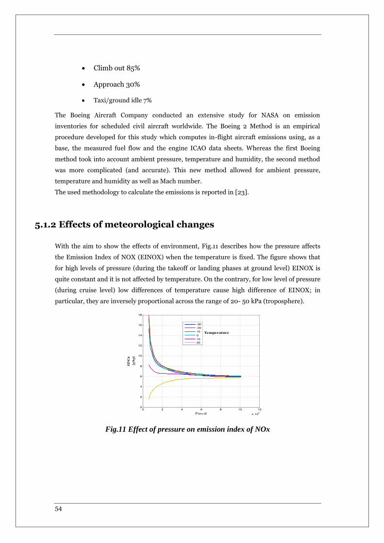
54

Climb out 85%

Approach 30%

Taxi/ground idle 7%

The Boeing Aircraft Company conducted an extensive study for NASA on emission

inventories for scheduled civil aircraft worldwide. The Boeing 2 Method is an empirical

procedure developed for this study which computes in-flight aircraft emissions using, as a

base, the measured fuel flow and the engine ICAO data sheets. Whereas the first Boeing

method took into account ambient pressure, temperature and humidity, the second method

was more complicated (and accurate). This new method allowed for ambient pressure,

temperature and humidity as well as Mach number.

The used methodology to calculate the emissions is reported in [23].

5.1.2 Effects of meteorological changes

With the aim to show the effects of environment, Fig.11 describes how the pressure affects

the Emission Index of NOX (EINOX) when the temperature is fixed. The figure shows that

for high levels of pressure (during the takeoff or landing phases at ground level) EINOX is

quite constant and it is not affected by temperature. On the contrary, for low level of pressure

(during cruise level) low differences of temperature cause high difference of EINOX; in

particular, they are inversely proportional across the range of 20- 50 kPa (troposphere).

Fig.11 Effect of pressure on emission index of NOx

55

5.1.3 Noise Model

There are various decibel scales used to define and measure sound in terms that can be

related to human perception. An important property of sound is its frequency spectrum – the

way that its acoustic energy is distributed across the audible frequency range (from 20 Hz to

20 kHz approximately). Two particular scales are important for aircraft noise - A-weighted

sound level and Tone-corrected Perceived Noise Level [31]. The A-weighting is a simple filter

applied to sound measurements which applies more or less emphasis to different frequencies

to mirror the frequency sensitivity of the human ear at moderate sound energy levels [72]. A-

weighted sound level is an almost universally used scale of environmental noise level: it is

used for most aircraft noise monitoring applications as well as for the description of road, rail

and industrial noise. A-weighted levels are usually denoted as LA. The noise impact

assessments that generate the need for noise exposure contours generally rely on A-weighted

metrics and these are therefore of primary interest in this guidance; although there are

exceptions, Perceived Noise Level applications are confined mostly to aircraft design and

certification.

Noise metrics may be thought of as measures of noise ‘dose’. There are two main types,

describing (1) single noise events (Single Event Noise Metrics) and (2) total noise

experienced over longer time periods (Cumulative Noise Metrics).

Noise levels are usually defined at fixed observer locations or mapped as contours (i.e. iso-

lines) depicting the area where the specified levels are exceeded. They are used – especially

cumulative metrics - in all domains of transportation noise, in our case air-traffic. These are

used to describe the acoustic event caused by a single aircraft movement. Two types are in

common usage, both can be determined by measurements as well as by calculations using

suitable models (that are the principle subject of this guidance). They are (1) Lmax, based on

(1) the maximum sound intensity during the event and (2) LE, based on the total sound

energy in the event. The total sound energy can be expressed as the product of the maximum

sound intensity and an ‘effective duration’ of the event.

An aircraft noise event can be described by its observed level-time-history L(t). These are the

maximum (frequencyweighted) sound level Lmax and a duration t. Common definitions of

the duration are the effective duration, te, i.e. the duration of a noise event with the constant

level Lmax that contains the same sound energy as the noise event described by the level-

time-history L(t).

Three corresponding single event metrics of particular importance in aircraft noise [73,

74, 75] are (1) Maximum A-weighted Sound level (abbreviation LAmax), (2) Sound Exposure

Level (acronym SEL, abbreviation LAE) and (3) Effective Perceived Noise Level (acronym

EPNL, abbreviation LEPN).

56

LAmax is still the favored metric for day to day noise monitoring at airports. EPNL is the

metric for aircraft noise certification limits laid down by ICAO Annex 16 [75], which all new

civil aircraft have to meet. Certification gives noise levels at specific points rather than

information on the total noise in the general vicinity of the flight path. An indication of the

latter is provided by contours of constant single event noise level - so-called “noise

footprints”. Noise footprints are useful performance indicators for noise abatement flight

procedures since they reflect the impact of noise on the ground of the whole flight path (flight

altitude, engine power setting and aircraft speed at all points) rather than only from a part of

it. As the decibel scale is logarithmic, long term aircraft noise exposure indices can be

logically and conveniently expressed in the form L+ K lg N, where L is the average event level

(in decibels of some kind), N is the number of events during the time period of interest, and

K is a constant which quantifies the relative importance of noise level and number.

5.1.4 Weather data

In order to compute emissions, the vertical distribution of the following meteorological data

is needed: density of air, pressure, temperature, relative humidity, wind speed and direction,

and clouds position. These data, except density of the air, are available through numerical

weather models that several weather organizations in the world develop for analysis of

current situations and forecasts. In our test, only density of the air is computed using the

International Standard Atmosphere (ISA) formula.

In the U.S.A., these data are public domain and several different models are available over

the Internet, with archives containing all of the data day by day. Among these we chose to use

the Rapid Refresh (RAP). The RAP is a NOAA/NCEP operational weather prediction system

running every hour that replaced the Rapid Update Cycle (RUC) on 1 May 2012. The RAP is

an atmospheric prediction system that consists primarily of a numerical forecast model and

an analysis system to initialize the model. Models run hourly, with analysis and hourly

forecasts out to 18 hours. RAP files are stored in the GRIB2 file format. GRIB (GRIdded

Binary) is a mathematically concise data format commonly used in meteorology to store

historical and forecast weather data. The minimum grid spatial resolution is 13 km. In

particular, we use a pgrb GRIB2 file that uses 37 vertical levels (isobaric levels) with a grid

having a horizontal spatial resolution of 20 km with a dimension of 225x301 grid cells. In

order to define clouds, we use the radar reflectivity value.

RAP data can be downloaded from an archive containing datasets for each day/hour of the

latest month. Each GRIB file contains the analysis of weather data as it was at that day/hour

and the 18 forecasts for the following 18 hours.

57

This allowed us to evaluate the accuracy of the forecasts by comparing, for example, the

weather forecast of 5 p.m. as produced at 3 p.m., with the “real” weather as it was seen in the

analysis made at 5 p.m. (2-hour forecast).

5.1.5 Aircraft model

There are several models that can be used to describe an aircraft movement, in accordance to

ref. [16,19,21,26] we consider the aircraft, in a 3 Dimension (3D) space with the position

described by latitude, longitude and altitude.

Moreover, to obtain a path that minimizes the pollutant emissions, more parameters have to

be added to the aircraft description.

The aircraft is modeled as an automaton , where:

- X is the finite set of states,

- E is a finite set of events,

- δ is the transition function, described by a state transition directed graph (digraph)

G=(X, A) where X= is the set of nodes , representing all the states

of the aircraft in the considered time slice and A={a_ij } is the set of directed arcs,

representing the possible transitions of the aircraft.

- X_0 is the initial state,

- X_m is the set of final states,

- f is the output function that associates to each state and each event a

vector of n components.

The automaton state X is a vector of K components describing the

aircraft position and dynamics.

Here, we consider the following K=5 components of the automaton state :

), , , ,

).

The first three variables are required to determine the current position of the aircraft in the

space (latitude, longitude and altitude) and the other two components describe the aircraft

dynamics aspects (true airspeed and heading).

Such five variables, that in general can assume continuous values, are discretized and, in the

adaptive grid, they will be modified to find the smallest graph that can provide accurate

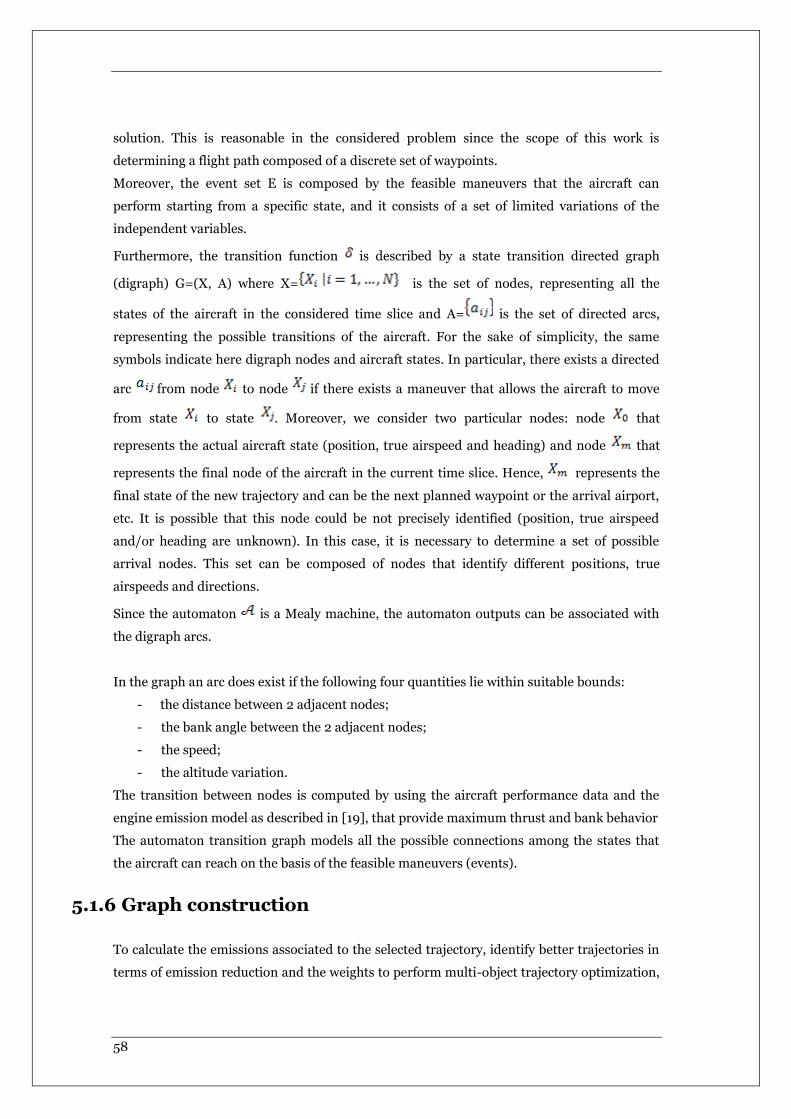
58

solution. This is reasonable in the considered problem since the scope of this work is

determining a flight path composed of a discrete set of waypoints.

Moreover, the event set E is composed by the feasible maneuvers that the aircraft can

perform starting from a specific state, and it consists of a set of limited variations of the

independent variables.

Furthermore, the transition function is described by a state transition directed graph

(digraph) G=(X, A) where X= is the set of nodes, representing all the

states of the aircraft in the considered time slice and A= is the set of directed arcs,

representing the possible transitions of the aircraft. For the sake of simplicity, the same

symbols indicate here digraph nodes and aircraft states. In particular, there exists a directed

arc from node to node if there exists a maneuver that allows the aircraft to move

from state to state . Moreover, we consider two particular nodes: node that

represents the actual aircraft state (position, true airspeed and heading) and node that

represents the final node of the aircraft in the current time slice. Hence, represents the

final state of the new trajectory and can be the next planned waypoint or the arrival airport,

etc. It is possible that this node could be not precisely identified (position, true airspeed

and/or heading are unknown). In this case, it is necessary to determine a set of possible

arrival nodes. This set can be composed of nodes that identify different positions, true

airspeeds and directions.

Since the automaton is a Mealy machine, the automaton outputs can be associated with

the digraph arcs.

In the graph an arc does exist if the following four quantities lie within suitable bounds:

- the distance between 2 adjacent nodes;

- the bank angle between the 2 adjacent nodes;

- the speed;

- the altitude variation.

The transition between nodes is computed by using the aircraft performance data and the

engine emission model as described in [19], that provide maximum thrust and bank behavior

The automaton transition graph models all the possible connections among the states that

the aircraft can reach on the basis of the feasible maneuvers (events).

5.1.6 Graph construction

To calculate the emissions associated to the selected trajectory, identify better trajectories in

terms of emission reduction and the weights to perform multi-object trajectory optimization,

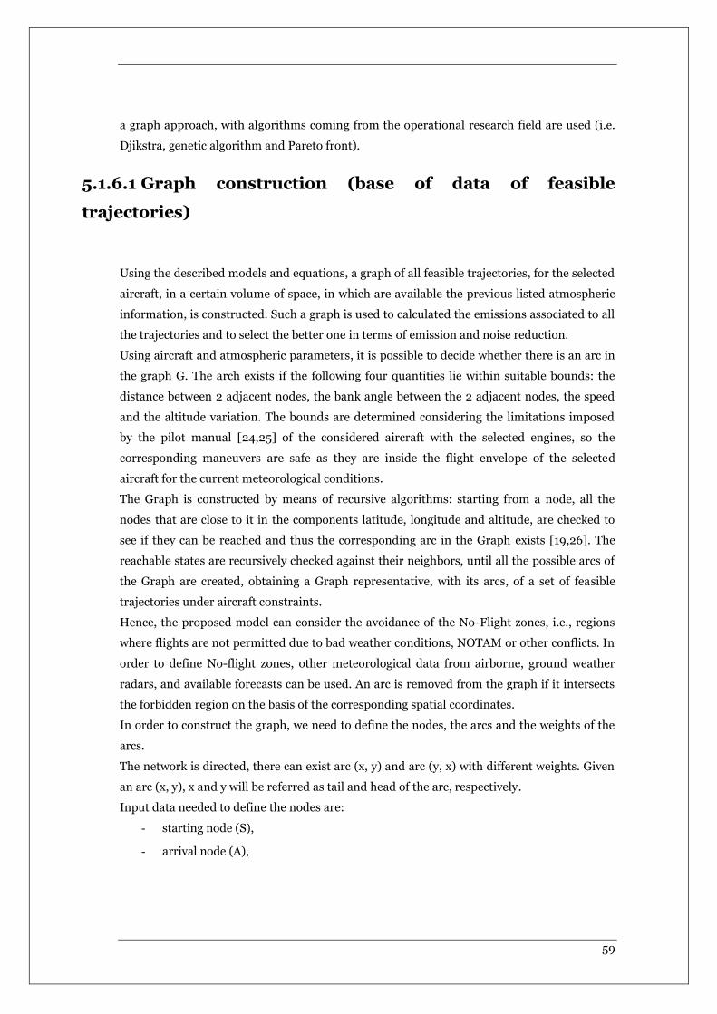
59

a graph approach, with algorithms coming from the operational research field are used (i.e.

Djikstra, genetic algorithm and Pareto front).

5.1.6.1 Graph construction (base of data of feasible

trajectories)

Using the described models and equations, a graph of all feasible trajectories, for the selected

aircraft, in a certain volume of space, in which are available the previous listed atmospheric

information, is constructed. Such a graph is used to calculated the emissions associated to all

the trajectories and to select the better one in terms of emission and noise reduction.

Using aircraft and atmospheric parameters, it is possible to decide whether there is an arc in

the graph G. The arch exists if the following four quantities lie within suitable bounds: the

distance between 2 adjacent nodes, the bank angle between the 2 adjacent nodes, the speed

and the altitude variation. The bounds are determined considering the limitations imposed

by the pilot manual [24,25] of the considered aircraft with the selected engines, so the

corresponding maneuvers are safe as they are inside the flight envelope of the selected

aircraft for the current meteorological conditions.

The Graph is constructed by means of recursive algorithms: starting from a node, all the

nodes that are close to it in the components latitude, longitude and altitude, are checked to

see if they can be reached and thus the corresponding arc in the Graph exists [19,26]. The

reachable states are recursively checked against their neighbors, until all the possible arcs of

the Graph are created, obtaining a Graph representative, with its arcs, of a set of feasible

trajectories under aircraft constraints.

Hence, the proposed model can consider the avoidance of the No-Flight zones, i.e., regions

where flights are not permitted due to bad weather conditions, NOTAM or other conflicts. In

order to define No-flight zones, other meteorological data from airborne, ground weather

radars, and available forecasts can be used. An arc is removed from the graph if it intersects

the forbidden region on the basis of the corresponding spatial coordinates.

In order to construct the graph, we need to define the nodes, the arcs and the weights of the

arcs.

The network is directed, there can exist arc (x, y) and arc (y, x) with different weights. Given

an arc (x, y), x and y will be referred as tail and head of the arc, respectively.

Input data needed to define the nodes are:

- starting node (S),

- arrival node (A),

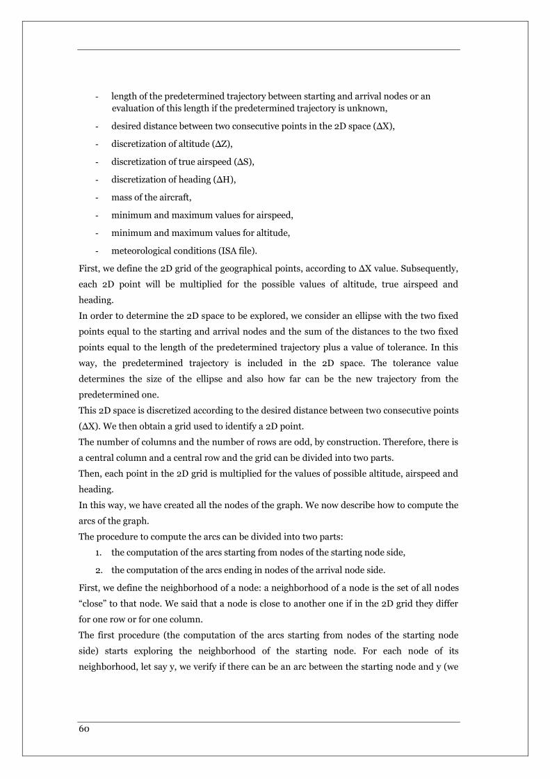
60

- length of the predetermined trajectory between starting and arrival nodes or an

evaluation of this length if the predetermined trajectory is unknown,

- desired distance between two consecutive points in the 2D space (ΔX),

- discretization of altitude (ΔZ),

- discretization of true airspeed (ΔS),

- discretization of heading (ΔH),

- mass of the aircraft,

- minimum and maximum values for airspeed,

- minimum and maximum values for altitude,

- meteorological conditions (ISA file).

First, we define the 2D grid of the geographical points, according to ΔX value. Subsequently,

each 2D point will be multiplied for the possible values of altitude, true airspeed and

heading.

In order to determine the 2D space to be explored, we consider an ellipse with the two fixed

points equal to the starting and arrival nodes and the sum of the distances to the two fixed

points equal to the length of the predetermined trajectory plus a value of tolerance. In this

way, the predetermined trajectory is included in the 2D space. The tolerance value

determines the size of the ellipse and also how far can be the new trajectory from the

predetermined one.

This 2D space is discretized according to the desired distance between two consecutive points

(ΔX). We then obtain a grid used to identify a 2D point.

The number of columns and the number of rows are odd, by construction. Therefore, there is

a central column and a central row and the grid can be divided into two parts.

Then, each point in the 2D grid is multiplied for the values of possible altitude, airspeed and

heading.

In this way, we have created all the nodes of the graph. We now describe how to compute the

arcs of the graph.

The procedure to compute the arcs can be divided into two parts:

1. the computation of the arcs starting from nodes of the starting node side,

2. the computation of the arcs ending in nodes of the arrival node side.

First, we define the neighborhood of a node: a neighborhood of a node is the set of all nodes

“close” to that node. We said that a node is close to another one if in the 2D grid they differ

for one row or for one column.

The first procedure (the computation of the arcs starting from nodes of the starting node

side) starts exploring the neighborhood of the starting node. For each node of its

neighborhood, let say y, we verify if there can be an arc between the starting node and y (we

61

will explain later how to verify if an arc exists). If the arc exists it is added to the network and,

if node y satisfies some constraints, it is saved as node to be explored. After the exploration of

all nodes of the neighborhood of the starting node, we choose a node to be explored and we

repeat the same procedure (exploration of all nodes of its neighborhood). The procedure

ends when there are no nodes to be explored.

The second procedure (the computation of the arcs ending in nodes of the arrival node side)

is similar to the first procedure. We still explore a neighborhood, but a node has to satisfy

other constraints to be saved as node to be explored. We start exploring the neighborhood of

the arrival node, verifying if from a node of its neighborhood the arrival node can be reached.

If it is the case, the arc is added to the network and the node, if it satisfies some constraints,

is saved as node to be explored.

In general, a node can be inserted between the node to be explored if it has not been explored

and if it is in the starting node side (first procedure) or in the arrival node side (second

procedure).

The computation of the weights of the arcs is connected with the check if an arc exists.

For each couple of nodes, we compute the needed thrust to fly between the two nodes.

Subsequently, given the thrust and other meteorological parameters it is possible to compute

emissions.

We now describe the procedure to compute the needed thrust between two nodes.

3. compute the distance between the two nodes given the coordinates and the altitude.

4. compute the course angle between the two points (direction to be followed)

5. compute the average of true airspeed

6. compute ground speed and correction angle (due to wind) using course angle, average

true airspeed and wind data (speed and direction)

7. compute travel time given ground speed and distance

8. compute correction of heading given the current heading and the correction angle

9. compute rate of turn given heading variation and travel time of the arc

10. compute bank angle given rate of turn and average true airspeed

11. compute thrust given distance, true airspeed in the two nodes, altitude in the two

nodes, bank angle, travel time, flight phase, mass of the aircraft and meteorological

parameters.

Each component of the state vector are parametrized taking into account min value, max

value, step resolution named respectively, for i: 1..5, XiMin; XiMax; DXi. To determine the

better graph in terms of minimum dimensions for the required accuracy all the previous

parameters will be automatically varied till some stop criteria will be reached.

The chosen stop criteria are:

- DXi reached selected thresholds depending on the phase of flight;

62

- The fuel consumption doesn’t increase anymore for 3 consecutive steps

- The mean and mode of the maximum and minimum altitude doesn’t increase for 3

consecutive steps.

In the following picture is represented a typical aircraft trajectory with the variables limits

(XiMin; XiMax).

Fig.12 Aircraft trajectory with A320 typical performance parameters (maximum

and Minimum speed, altitude, climb time and distance)

5.1.6.2 Dijkstra based trajectory optimizer

Dijkstra’s algorithm finds the shortest path from the source node v1 to all other nodes in

a network with nonnegative arc weights [29]. Dijkstra’s algorithm maintains a distance label

d(i) with each node i, which is an upper bound on the shortest path cost to node i.

At any intermediate step, the algorithm divides the nodes into two groups: those which it

designates as permanently labeled (or permanent) and those it designates as temporarily

labeled (or temporary). The distance label to any permanent node represents the shortest

distance from the source to that node. For any temporary node, the distance label is an upper

bound on the shortest path distance to that node.

The basic idea of the algorithm is to fan out from node v1 and permanently label nodes in the

order of their distances from node v1. Initially, we give node v1 a permanent label of zero,

and each other node j a temporary label equal to ∞. At each iteration, the label of a node i is

its shortest distance from the source node along a path whose internal nodes (i.e., nodes

other than v1 or the node i itself) are all permanently labeled.

63

The algorithm selects a node i with the minimum temporary label, makes it permanent, and

reaches out from that node, that is, scans arcs in A(i) (arcs outgoing from node i) to update

the distance labels of adjacent nodes.

The algorithm terminates when it has designated all nodes as permanent. The correctness of

the algorithm relies on the key observation that we can always designate the node with

minimum temporary label as permanent.

The pseudo-code of Dijkstra’s algorithm is report in the following:

5.1.6.3 Genetic based trajectory optimizer

The genetic optimization algorithm is a search heuristic algorithm simulating the

process of natural evolution. This algorithm is routinely used to generate useful solutions to

searching and optimization problems. Genetic algorithms belong to the larger class of

Evolutionary Algorithms (EA) generating solutions to optimization problems using several

methods inspired by natural evolution, such as inheritance, mutation, selection, and

crossover.

In a genetic optimization algorithm, a population of strings (called chromosomes or the

genotype of the genome), which encode candidate solutions (called individuals, creatures, or

phenotypes) to an optimization problem, evolves toward better solutions. Traditionally,

solutions are represented in binary format as strings of 0s and 1s, but other encoding

methods may be used. The evolution usually starts from a population of randomly generated

individuals and happens in generations. In each generation, the fitness of every individual in

the population is evaluated, multiple individuals are stochastically selected from the current

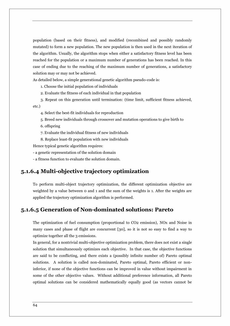
64

population (based on their fitness), and modified (recombined and possibly randomly

mutated) to form a new population. The new population is then used in the next iteration of

the algorithm. Usually, the algorithm stops when either a satisfactory fitness level has been

reached for the population or a maximum number of generations has been reached. In this

case of ending due to the reaching of the maximum number of generations, a satisfactory

solution may or may not be achieved.

As detailed below, a simple generational genetic algorithm pseudo-code is:

1. Choose the initial population of individuals

2. Evaluate the fitness of each individual in that population

3. Repeat on this generation until termination: (time limit, sufficient fitness achieved,

etc.)

4. Select the best-fit individuals for reproduction

5. Breed new individuals through crossover and mutation operations to give birth to

6. offspring

7. Evaluate the individual fitness of new individuals

8. Replace least-fit population with new individuals

Hence typical genetic algorithm requires:

- a genetic representation of the solution domain

- a fitness function to evaluate the solution domain.

5.1.6.4 Multi-objective trajectory optimization

To perform multi-object trajectory optimization, the different optimization objective are

weighted by a value between 0 and 1 and the sum of the weights is 1. After the weights are

applied the trajectory optimization algorithm is performed.

5.1.6.5 Generation of Non-dominated solutions: Pareto

The optimization of fuel consumption (proportional to CO2 emission), NOx and Noise in

many cases and phase of flight are concurrent [30], so it is not so easy to find a way to

optimize together all the 3 emissions.

In general, for a nontrivial multi-objective optimization problem, there does not exist a single

solution that simultaneously optimizes each objective. In that case, the objective functions

are said to be conflicting, and there exists a (possibly infinite number of) Pareto optimal

solutions. A solution is called non-dominated, Pareto optimal, Pareto efficient or non-

inferior, if none of the objective functions can be improved in value without impairment in

some of the other objective values. Without additional preference information, all Pareto

optimal solutions can be considered mathematically equally good (as vectors cannot be

65

ordered completely). The set of Pareto optimal solutions is often called the Pareto front. The

methodology proposed in this thesis aims at combining the set of emissions computed during

a flight phase (the results in climb phase are reported below), considering the aircraft

moving from an initial waypoint toward a final waypoint. The emissions, that typically

have different units of measurement and different ranges, have been normalized

considering the typical range of emissions in that flight phase as described in the

ICAO databank for CO2 [27,28], the Boeing model for NOX [23] and the DOC29 [34] for

Noise. The aircraft model used in the simulation is derived by BADA database [21] for

A320. The optimized trajectory is then used to compute the emissions in climb phase

given that set of weights. Changing the set of weights at the input and computing the

corresponding optimized trajectories and related emissions, it is possible to determined

what set of weights produces non-dominated Pareto solution. Repeating this

computation on different flights and different weather condition, it is possible to study

what is the best set of weights for that type of aircraft. The main contribution of this

thesis is to investigate the optimal values for the emissions weights in a specific climb

phase. In general more than one solution was obtained and the decision maker,

typically the flight company, can choose which pollutant is more important to be

reduced in that flight area and determine the cost index.

The Pareto optimal solution method is tested on the climb phase of the trajectory of

an A320, DAL1451 (from Flightaware), in USA and using the real atmospheric condition

contained in a GRIB file downloaded from NOAA database to calculate the emissions. The

multi-objective function was computed using a linear combination of the three pollutants:

CO2, NOx and Noise. The weights for each pollutant in the optimization algorithm are

chosen between 0.1 and 0.8 and the sum of the three weights is one.

66

CHAPTER 6 RESULTS

OF TRAJECTORY

OPTIMIZER APPLIED

TO REAL SCENARIOS

WITH UNFORESEEN

WEATHER EVENTS

In the present section are reported different kind of results related to the proposed trajectory

optimizer. In the first part the weather prediction reliability is considered. It is demonstrated

that the weather predictions (especially the weather reflectivity and the wind) are not enough

reliable for a preplanned optimized trajectory, but it is necessary to provide an on-board real

time trajectory optimization. Then two use cases, in real conditions, with an A320 in climb

and in cruise phases, are analyzed, the optimized trajectories, with different optimization

target, are provided and the results are compared with the real flight, showing the possibility

of a big potential emission reduction improvements. Then the multi-objective trajectory

optimizer is considered and the different emission results associated to the optimized

trajectories obtained with different emission weights, are provided, and compared. Set of

emission weights that provided the same results in terms of emissions, and that provided the

minimum emissions of the selected pullant, are identified. Then the obtained using different

weather models are compared and the different results are underlined. Finally, it is proposed

67

a flight simulator, based on X-Plane, as tool to validate the data. As it is shown later, the

results obtained are quite promising.

For the calculation, only aircraft climb and cruise phases are taken into account, because

they are the only one in which it is possible to obtain a relevant decrease of fuel consumption

and emissions, while in descent phase generally the pilot perform a continuous descent

approach with the engine in idle mode, so there are no big margins of possible

improvements.

6.1 Weather prediction reliability

As mentioned before, trajectory optimization is highly sensitive to weather conditions;

pressure, relative humidity, wind intensity and direction have various influences on thrust

conditions and emissions [19]. In this section, real atmospheric conditions and real flight

trajectory are used to evaluate the performance of our algorithm for trajectory optimization

and to calculate and compare emissions associated to different trajectories (real one and

optimized ones). In particular, some test cases, related to different phase of flight and based

on real data downloaded from USA internet archives, are described and the results, of the

application of optimizer to these test cases, are reported.

The reference weather models used to define the following test cases are the ones produced

by the National Oceanic and Atmospheric Administration (NOAA), a U.S.A. federal agency

focused on the condition of the oceans and the atmosphere. They distribute several weather

model datasets [11] upon different domains and most data, due to U.S. federal law, are

available as public domain.

From the NOAA archives, the RAP (Rapid Refresh) hourly-updated model weather

prediction was used. RAP model and its data are most likely the state of the art regarding

reliable weather information for aircraft use available as public domain.

In the following test cases, we used RAP weather datasets with 20 Km spatial resolution and

50 altitude levels, downloaded from the NOAA archive that contains datasets for each

day/hour of the latest month. Each GRIB (Gridded Binary) file contains the analysis of

weather data as it was at that day/hour and the 18 forecasts for the following 18 hours. That

allows to evaluate the accuracy of the forecasts, by comparing the predicted weather forecast,

referred to different hours, with the “real” weather. The days evaluated are 17/18/19/20 June

2012, the results are reported below and they show that for some parameters (T, P, etc.) the

predictions are reliable, for other parameters (reflectivity, wind) more than 1h predictions

are not reliable and it shouldn’t be used for trajectory optimization. These unpredictable

parameters produce the “unforeseen” weather events the pilot should cope with. Unforeseen

68

reflectivity and wind changes are some of the events used to start Q-AI for trajectory

optimization calculations.

6.1.1 evaluation of weather prediction Accuracy

Weather reflectivity and wind (speed and direction) are 2 of the events that starts Q-AI

calculation and are used for trajectory optimization. These data can be obtained from a

webserver or on-board from weather radar (reflectivity and radial wind intensity).

The reflectivity provided by the radar is usually described by colour or level. The colours in a

radar image normally range from blue or green for weak returns, to red or magenta for very

strong returns. The numbers in a verbal report increase with the severity of the returns. For

example, the U.S. National Doppler Radar sites use the following scale for different levels of

reflectivity:

- magenta: 65 dBZ (extremely heavy precipitation, possible hail)

- red: 52 dBZ

- yellow: 36 dBZ

- green: 20 dBZ (light precipitation)

Strong returns (red or magenta) may indicate not only heavy rain but also thunderstorms,

hail, strong winds, or tornadoes, but they need to be interpreted carefully (annex A).

When describing weather radar returns, pilots, dispatchers, and air traffic controllers will

typically refer to three return levels:

- level 1 corresponds to a green radar return, indicating usually light precipitation and

little to no turbulence, leading to a possibility of reduced visibility.

- level 2 corresponds to a yellow radar return, indicating moderate precipitation,

leading to the possibility of very low visibility, moderate turbulence and an

uncomfortable ride for aircraft passengers.

- level 3 corresponds to a red radar return, indicating heavy precipitation, leading to

the possibility of thunderstorms and severe turbulence and serious structural

damage to the aircraft.

An example of the parameter “MaximumComposite_Radar_Reflectivity”, taken from the

GRIB file for 18/6/2012 at 3 a.m (current weather field), is shown in the figure 1 below. In

the figure the reflectivity values are in dBZ and the colors follow the rainbow colormap values

at the right of the figure. The considered GRIB file was downloaded from NOAA site, in

particular from CONUS (Continental United States) domain for RAP model with 225x301

grid points.

69

Fig.13 Weather reflectivity on USA the 18/6/2012 at 3 a.m

6.1.1.1 Reflectivity forecast accuracy

In order to evaluate accuracy of forecasts regarding evaluation of the presence of bad weather

(level 1, reflectivity > 20 dBZ), or potentially severe weather condition (level 2 or more, then

reflectivity level > 36 dBZ), a threshold filter was applied to reflectivity data (current data

and forecasted ones related to the same hour) to select regions with reflectivity above 20 dBZ

(fig 3) and above 36 dBz.

In figures below an example of a rainbow color map representation analysis, of current

weather at 10 a.m. 19/06/2012, and the 1-hour forecast made at 9 a.m, is reported (Fig. 14).

Weather analysis Vs. forecast: dBZ values

Analisys at 10 a.m. 1 Hour forecast at 9 a.m.

70

Fig.14 Real and forecasted reflectivity on USA the 18/6/2012 at 3 a.m

In the following figure are represented the same data with the reflectivity threshold of 20 dBz

applied.

Weather analysis Vs. forecast: 20 dBZ threshold

Analisys at 10 a.m. 1 Hour forecast at 9 a.m.

Fig.15 Real and forecasted reflectivity above 20 dBz on USA the 18/6/2012

at 3 a.m

Comparing the two images it is possible to identify a large zone with high reflectivity that in

forecast was “clear”. Conventionally this situation is called a “miss” of FN: “False Negative”.

In other examples, instead, it was possible to idenfify zones with high reflectivity forecast

that in real weather (analysis) resulted clear (“false alarm”, conventionally called FP: “False

Positive”).

In the image below the comparison between the 2 previous images is reported (in red the

“perfect forecast” or TP: True Positive, in cyan the difference).

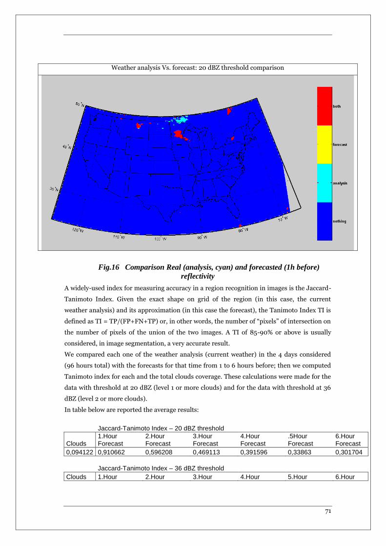
71

Weather analysis Vs. forecast: 20 dBZ threshold comparison

Fig.16 Comparison Real (analysis, cyan) and forecasted (1h before)

reflectivity

A widely-used index for measuring accuracy in a region recognition in images is the Jaccard-

Tanimoto Index. Given the exact shape on grid of the region (in this case, the current

weather analysis) and its approximation (in this case the forecast), the Tanimoto Index TI is

defined as TI = TP/(FP+FN+TP) or, in other words, the number of “pixels” of intersection on

the number of pixels of the union of the two images. A TI of 85-90% or above is usually

considered, in image segmentation, a very accurate result.

We compared each one of the weather analysis (current weather) in the 4 days considered

(96 hours total) with the forecasts for that time from 1 to 6 hours before; then we computed

Tanimoto index for each and the total clouds coverage. These calculations were made for the

data with threshold at 20 dBZ (level 1 or more clouds) and for the data with threshold at 36

dBZ (level 2 or more clouds).

In table below are reported the average results:

Jaccard-Tanimoto Index – 20 dBZ threshold

Clouds 1.Hour Forecast

2.Hour Forecast

3.Hour Forecast

4.Hour Forecast

.5Hour Forecast

6.Hour Forecast

0,094122 0,910662 0,596208 0,469113 0,391596 0,33863 0,301704

Jaccard-Tanimoto Index – 36 dBZ threshold

Clouds 1.Hour 2.Hour 3.Hour 4.Hour 5.Hour 6.Hour

72

Forecast Forecast Forecast Forecast Forecast Forecast

0,004701 0,812975 0,433031 0,260201 0,159075 0,099386 0,067976

Table 2 Clouds reflectivity prediction reliability

It can be seen that the weather forecast accuracy at 1 hour is quite good, but it becomes much

worse very quickly. Only forecasts not older than 1 hour should be used in order to plan

trajectories with a reliable knowledge about the “no flight zones” due to severe weather

conditions.

6.1.1.2 Wind forecast accuracy

The same calculations were done also for wind direction and speed in the same days

(applying a threshold to wind speed and direction to evaluate the changes). The data were

selected from the same GRIB files used before. The results present a behavior, in data

prediction accuracy over time, similar to the reflectivity.

6.2 Trajectory optimization Test cases

In this paragraph are considered 2 test cases (in climb and cruise phases) that will be

considered also in Chapter 7 for the real-time graph generation proposed method. The 2 test

cases consist in real flights of civil aircraft in real weather conditions. The emissions related

to the optimized trajectories are compared with the emissions related to the real trajectories

showing that there is a big margin of possible improvement.

6.2.1 Test Case 1

In this first test case is considered the real trajectory (downloaded from flightaware archive)

of an A320 (DAL1888) in cruise phase in real weather conditions (downloaded from NOAA

archive). In the following paragraphs, the emissions associated to the real aircraft trajectory

and the trajectories optimized in accordance to different criteria are provided and compared.

The considered trajectory is originated from the International Airport of Las Vegas (KLAS)

(36.080°, -115.152°) on November 11th 2012 at about 4 p.m. (UTC): DAL1888.

This flight is directed to the International Airport of Memphis. It is considered a part of the

cruise phase of the trajectories. We suppose that the mass of the aircraft is 64000 kg.

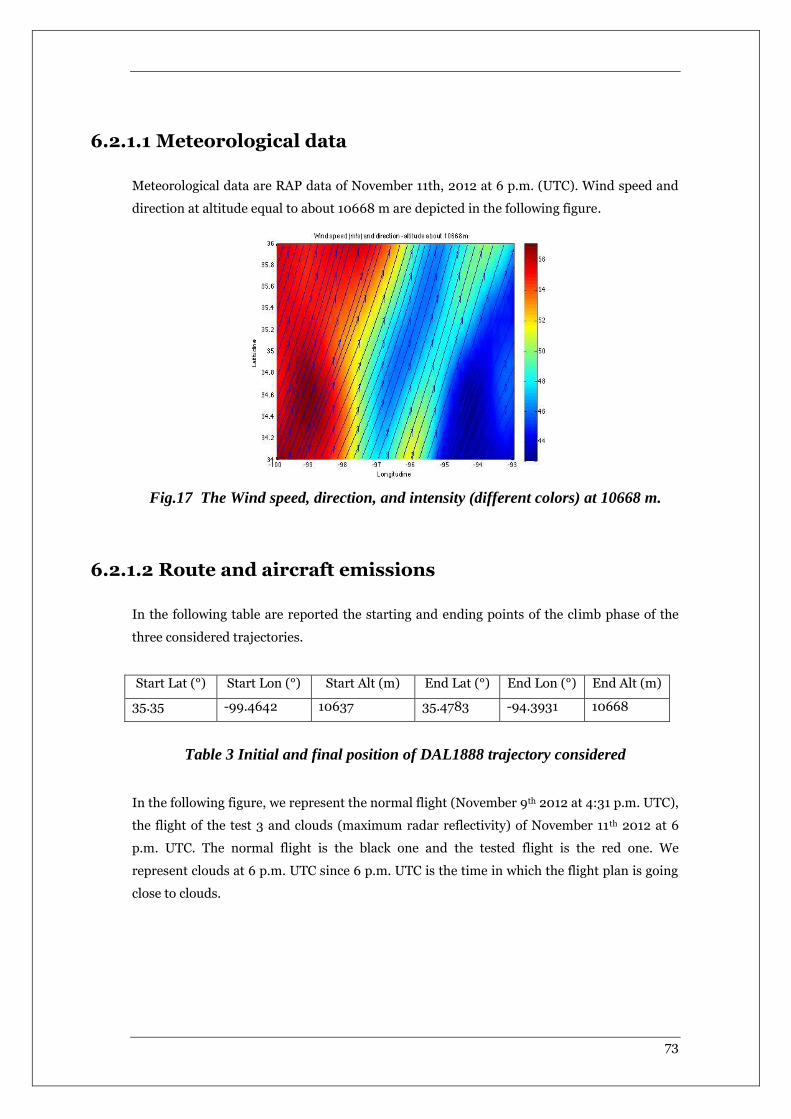
73

6.2.1.1 Meteorological data

Meteorological data are RAP data of November 11th, 2012 at 6 p.m. (UTC). Wind speed and

direction at altitude equal to about 10668 m are depicted in the following figure.

Fig.17 The Wind speed, direction, and intensity (different colors) at 10668 m.

6.2.1.2 Route and aircraft emissions

In the following table are reported the starting and ending points of the climb phase of the

three considered trajectories.

Start Lat (°) Start Lon (°) Start Alt (m) End Lat (°) End Lon (°) End Alt (m)

35.35 -99.4642 10637 35.4783 -94.3931 10668

Table 3 Initial and final position of DAL1888 trajectory considered

In the following figure, we represent the normal flight (November 9th 2012 at 4:31 p.m. UTC),

the flight of the test 3 and clouds (maximum radar reflectivity) of November 11th 2012 at 6

p.m. UTC. The normal flight is the black one and the tested flight is the red one. We

represent clouds at 6 p.m. UTC since 6 p.m. UTC is the time in which the flight plan is going

close to clouds.

74

Fig.18 DAL1888 real flights (black one usual, red one particular deviation tested)

In the following figure, we represent the same trajectories but clouds expected at 6 p.m. UTC

computed at 1 p.m. UTC (computed about 3 hours before the takeoff). From the figure one

can note that the normal trajectory flights close to dangerous clouds.

Fig.19 DAL1888 real flights (black one usual, red one tested)

In order to compute noise emissions three observation points are set: Minneapolis (44.993N,

-93.265E), St. Paul (44.9536N, -93.092E) and Rochester (44.031N, -92.467E).

75

The real trajectory is taken from "FlightAware" website (http://flightaware.com).

6.2.1.3 Test results

In the following table the aircraft emissions are reported. For the Multi-objective function

the weight of CO2 and NOx emissions is the same.

The differences in the calculated emissions depend mainly on wind and cloud reflectivity

values that are not so reliable for what concern the prediction [19]. On the other side,

pressure, temperature, and humidity prediction are more reliable [19].

Using the weighted Graph of the feasible trajectories, are calculated the emissions associated

to different trajectories. In table 3 are reported the emissions associated to the real flight

(column 2 in table 4) and the ones associated to optimized trajectories, applying Dijkstra

mono or multi-object and a genetic algorithm to select an optimized trajectory in accordance

to different criteria (table 4, in column 3 Dijkstra Mono-objective CO2, 4 Dijkstra Mono-

objective NOx, 5 Dijkstra Multi-objectives, 6 Genetic Multi-objective). The multi-objective

trajectory optimization is calculated attributing to NOx and CO2 emissions a weight of 0.5

each.

FA Dijkstra's algorithm GA

CO2 NOx MO MO

CO2 (kg) 4002 3472 3528 3528 3528

NOx (kg) 23.98 20.32 19.41 19.41 19.41

CPU time (s)

(network constr.)

3991

CPU time (s)

(optimization algorithm)

0.23 0.23 0.23 77.81

Table 4 DAL1888 emissions and emission associated to optimized trajectories

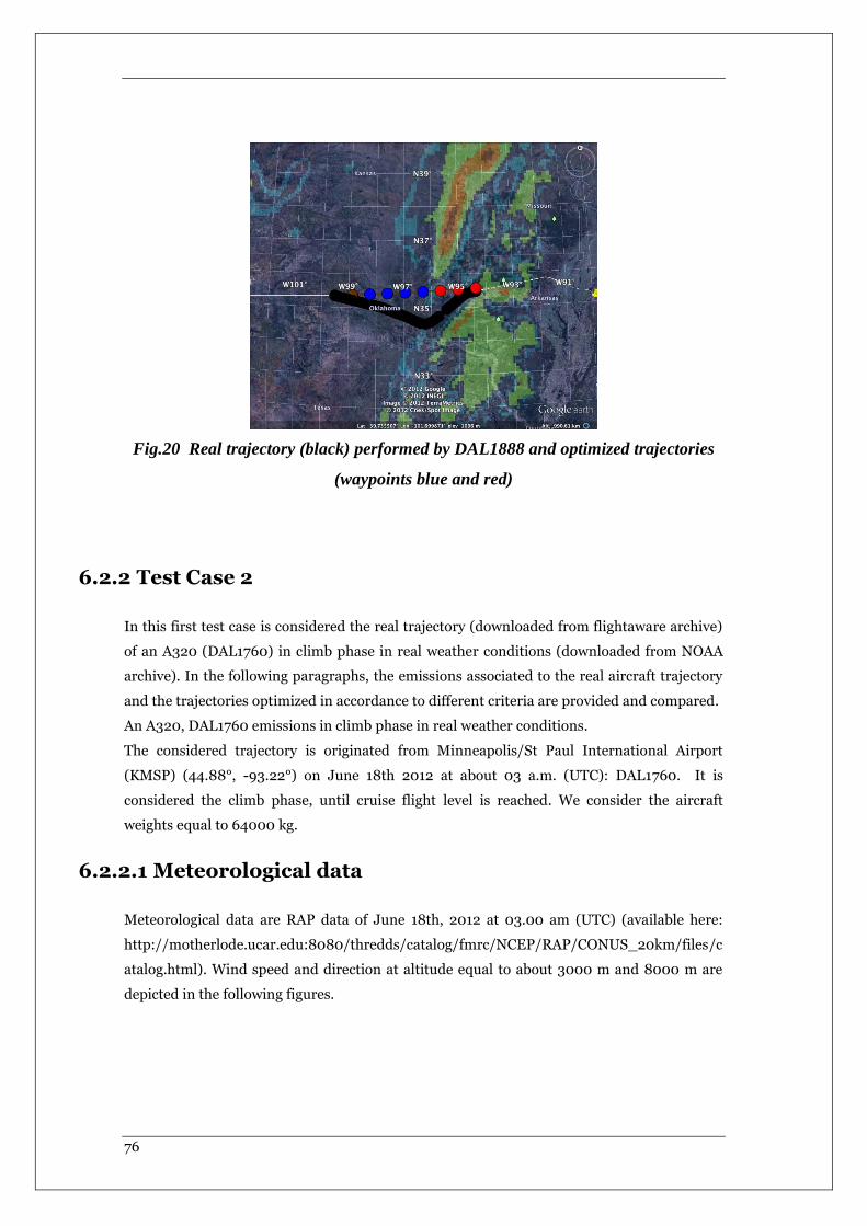
76

Fig.20 Real trajectory (black) performed by DAL1888 and optimized trajectories

(waypoints blue and red)

6.2.2 Test Case 2

In this first test case is considered the real trajectory (downloaded from flightaware archive)

of an A320 (DAL1760) in climb phase in real weather conditions (downloaded from NOAA

archive). In the following paragraphs, the emissions associated to the real aircraft trajectory

and the trajectories optimized in accordance to different criteria are provided and compared.

An A320, DAL1760 emissions in climb phase in real weather conditions.

The considered trajectory is originated from Minneapolis/St Paul International Airport

(KMSP) (44.88°, -93.22°) on June 18th 2012 at about 03 a.m. (UTC): DAL1760. It is

considered the climb phase, until cruise flight level is reached. We consider the aircraft

weights equal to 64000 kg.

6.2.2.1 Meteorological data

Meteorological data are RAP data of June 18th, 2012 at 03.00 am (UTC) (available here:

http://motherlode.ucar.edu:8080/thredds/catalog/fmrc/NCEP/RAP/CONUS_20km/files/c

atalog.html). Wind speed and direction at altitude equal to about 3000 m and 8000 m are

depicted in the following figures.

77

Fig.21 The Wind speed, direction and intensity (different colors) at 3000 m.

Fig.22 The Wind speed, direction and intensity (different colors) at 8000 m.

6.2.2.2 Route and aircraft emissions

In the following table are reported the starting and ending points of the climb phase of the

three considered trajectories.

Start Lat (°) Start Lon (°) Start Alt (m) End Lat (°) End Lon (°) End Alt (m)

44.8258 -93.2317 945 44.1100 -95.8472 10973

Table 5 Initial and final position of DAL1760 trajectory considered

In order to compute noise emissions three observation points are set: Minneapolis (44.993N,

-93.265E), St. Paul (44.9536N, -93.092E) and Rochester (44.031N, -92.467E).

The real trajectories are taken from "FlightAware" website (http://flightaware.com).

In the following figure (Fig.3) the "normal" trajectory (in this case the trajectory of June 17th

2012 at about 03 a.m.) (blue) and the trajectory of June 18th 2012 (black) are depicted,

related to real cloud reflectivity the June 18th 2012 at 03 a.m.

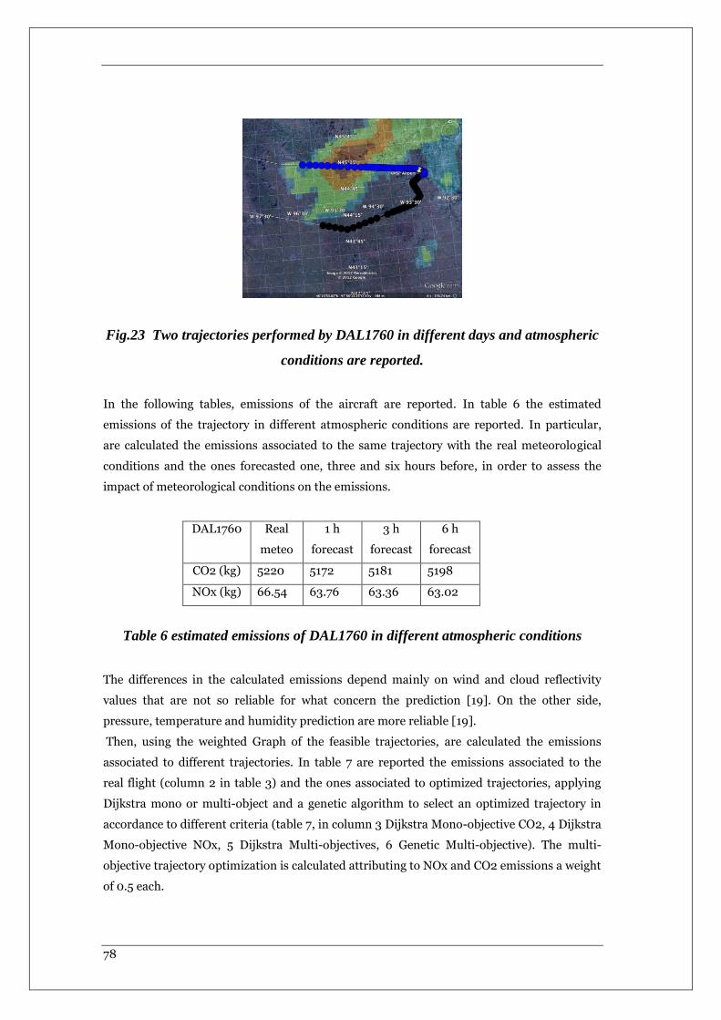
78

Fig.23 Two trajectories performed by DAL1760 in different days and atmospheric

conditions are reported.

In the following tables, emissions of the aircraft are reported. In table 6 the estimated

emissions of the trajectory in different atmospheric conditions are reported. In particular,

are calculated the emissions associated to the same trajectory with the real meteorological

conditions and the ones forecasted one, three and six hours before, in order to assess the

impact of meteorological conditions on the emissions.

DAL1760 Real

meteo

1 h

forecast

3 h

forecast

6 h

forecast

CO2 (kg) 5220 5172 5181 5198

NOx (kg) 66.54 63.76 63.36 63.02

Table 6 estimated emissions of DAL1760 in different atmospheric conditions

The differences in the calculated emissions depend mainly on wind and cloud reflectivity

values that are not so reliable for what concern the prediction [19]. On the other side,

pressure, temperature and humidity prediction are more reliable [19].

Then, using the weighted Graph of the feasible trajectories, are calculated the emissions

associated to different trajectories. In table 7 are reported the emissions associated to the

real flight (column 2 in table 3) and the ones associated to optimized trajectories, applying

Dijkstra mono or multi-object and a genetic algorithm to select an optimized trajectory in

accordance to different criteria (table 7, in column 3 Dijkstra Mono-objective CO2, 4 Dijkstra

Mono-objective NOx, 5 Dijkstra Multi-objectives, 6 Genetic Multi-objective). The multi-

objective trajectory optimization is calculated attributing to NOx and CO2 emissions a weight

of 0.5 each.

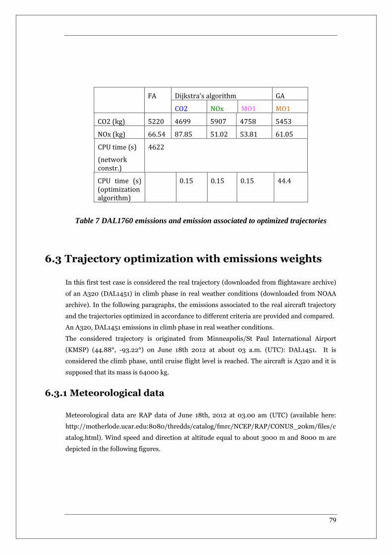
79

FA Dijkstra's algorithm GA

CO2 NOx MO1 MO1

CO2 (kg) 5220 4699 5907 4758 5453

NOx (kg) 66.54 87.85 51.02 53.81 61.05

CPU time (s)

(network constr.)

4622

CPU time (s) (optimization algorithm)

0.15 0.15 0.15 44.4

Table 7 DAL1760 emissions and emission associated to optimized trajectories

6.3 Trajectory optimization with emissions weights

In this first test case is considered the real trajectory (downloaded from flightaware archive)

of an A320 (DAL1451) in climb phase in real weather conditions (downloaded from NOAA

archive). In the following paragraphs, the emissions associated to the real aircraft trajectory

and the trajectories optimized in accordance to different criteria are provided and compared.

An A320, DAL1451 emissions in climb phase in real weather conditions.

The considered trajectory is originated from Minneapolis/St Paul International Airport

(KMSP) (44.88°, -93.22°) on June 18th 2012 at about 03 a.m. (UTC): DAL1451. It is

considered the climb phase, until cruise flight level is reached. The aircraft is A320 and it is

supposed that its mass is 64000 kg.

6.3.1 Meteorological data

Meteorological data are RAP data of June 18th, 2012 at 03.00 am (UTC) (available here:

http://motherlode.ucar.edu:8080/thredds/catalog/fmrc/NCEP/RAP/CONUS_20km/files/c

atalog.html). Wind speed and direction at altitude equal to about 3000 m and 8000 m are

depicted in the following figures.

80

Fig.24 The Wind speed, direction, and intensity (different colors) at 3000 m.

Fig.25 The Wind speed, direction, and intensity (different colors) at 8000 m.

6.3.2 Route and aircraft emissions

In the following table are reported the starting and ending points of the climb phase of the

three considered trajectories.

Start Lat (°) Start Lon (°) Start Alt (m) End Lat (°) End Lon (°) End Alt (m)

44.82 -93.23 914 43.33 -95.91 10363

Table 8 Initial and final position of DAL1451 trajectory considered

In order to compute noise emissions three observation points are set: Minneapolis (44.993N,

-93.265E), St. Paul (44.9536N, -93.092E) and Rochester (44.031N, -92.467E).

The real trajectories are taken from "FlightAware" website (http://flightaware.com).

In the following figure (Fig.3) the "normal" trajectory (in this case the trajectory of June 17th

2012 at about 03 a.m.) (blue) and the trajectory of June 18th 2012 (black) are depicted,

related to real cloud reflectivity the June 18th 2012 at 03 a.m.

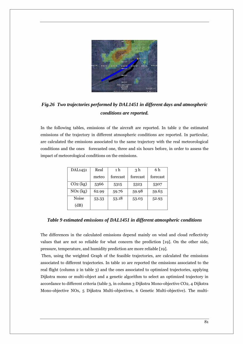
81

Fig.26 Two trajectories performed by DAL1451 in different days and atmospheric

conditions are reported.

In the following tables, emissions of the aircraft are reported. In table 2 the estimated

emissions of the trajectory in different atmospheric conditions are reported. In particular,

are calculated the emissions associated to the same trajectory with the real meteorological

conditions and the ones forecasted one, three and six hours before, in order to assess the

impact of meteorological conditions on the emissions.

DAL1451 Real

meteo

1 h

forecast

3 h

forecast

6 h

forecast

CO2 (kg) 5366 5315 5323 5307

NOx (kg) 62.99 59.76 59.98 59.63

Noise

(dB)

53.33 53.18 53.03 52.93

Table 9 estimated emissions of DAL1451 in different atmospheric conditions

The differences in the calculated emissions depend mainly on wind and cloud reflectivity

values that are not so reliable for what concern the prediction [19]. On the other side,

pressure, temperature, and humidity prediction are more reliable [19].

Then, using the weighted Graph of the feasible trajectories, are calculated the emissions

associated to different trajectories. In table 10 are reported the emissions associated to the

real flight (column 2 in table 3) and the ones associated to optimized trajectories, applying

Dijkstra mono or multi-object and a genetic algorithm to select an optimized trajectory in

accordance to different criteria (table 3, in column 3 Dijkstra Mono-objective CO2, 4 Dijkstra

Mono-objective NOx, 5 Dijkstra Multi-objectives, 6 Genetic Multi-objective). The multi-

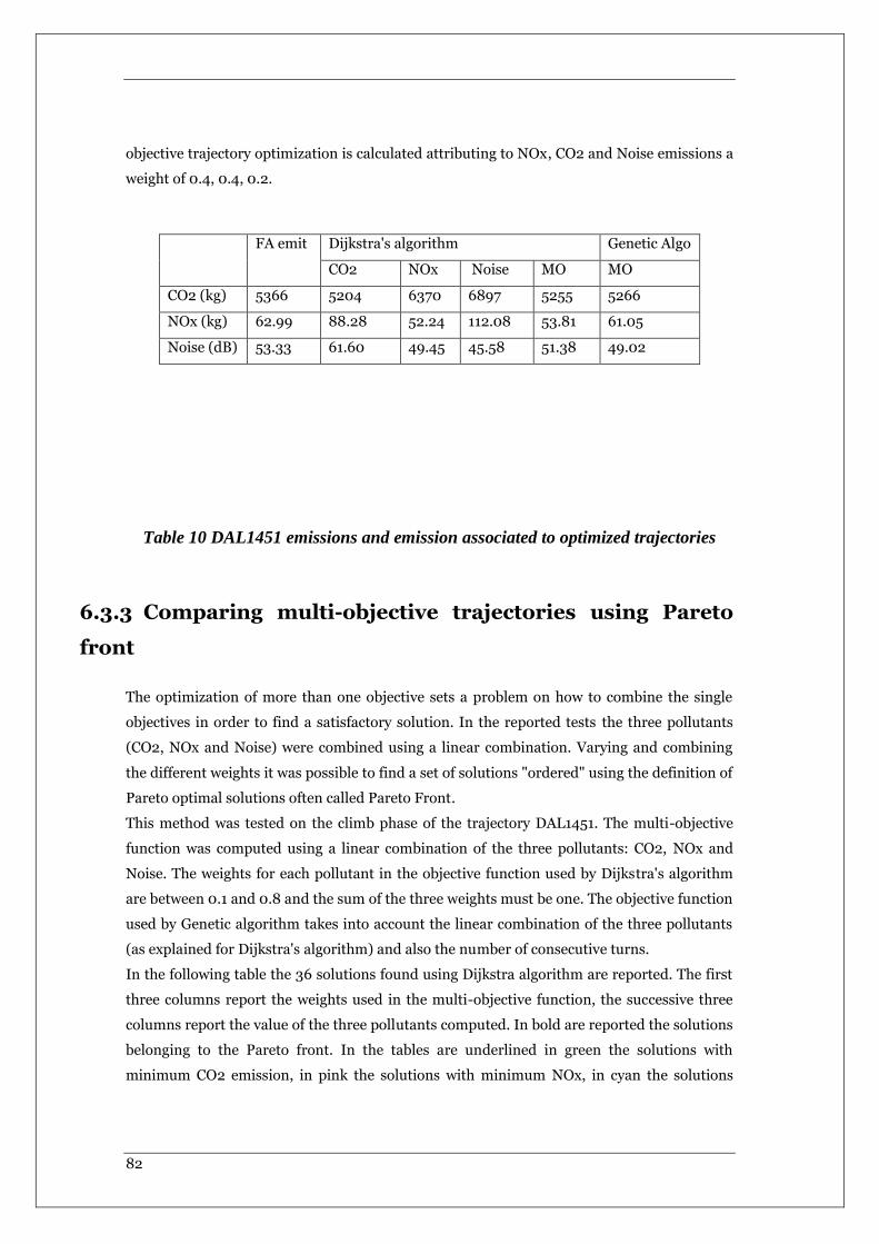
82

objective trajectory optimization is calculated attributing to NOx, CO2 and Noise emissions a

weight of 0.4, 0.4, 0.2.

Table 10 DAL1451 emissions and emission associated to optimized trajectories

6.3.3 Comparing multi-objective trajectories using Pareto

front

The optimization of more than one objective sets a problem on how to combine the single

objectives in order to find a satisfactory solution. In the reported tests the three pollutants

(CO2, NOx and Noise) were combined using a linear combination. Varying and combining

the different weights it was possible to find a set of solutions "ordered" using the definition of

Pareto optimal solutions often called Pareto Front.

This method was tested on the climb phase of the trajectory DAL1451. The multi-objective

function was computed using a linear combination of the three pollutants: CO2, NOx and

Noise. The weights for each pollutant in the objective function used by Dijkstra's algorithm

are between 0.1 and 0.8 and the sum of the three weights must be one. The objective function

used by Genetic algorithm takes into account the linear combination of the three pollutants

(as explained for Dijkstra's algorithm) and also the number of consecutive turns.

In the following table the 36 solutions found using Dijkstra algorithm are reported. The first

three columns report the weights used in the multi-objective function, the successive three

columns report the value of the three pollutants computed. In bold are reported the solutions

belonging to the Pareto front. In the tables are underlined in green the solutions with

minimum CO2 emission, in pink the solutions with minimum NOx, in cyan the solutions

FA emit Dijkstra's algorithm Genetic Algo

CO2 NOx Noise MO MO

CO2 (kg) 5366 5204 6370 6897 5255 5266

NOx (kg) 62.99 88.28 52.24 112.08 53.81 61.05

Noise (dB) 53.33 61.60 49.45 45.58 51.38 49.02

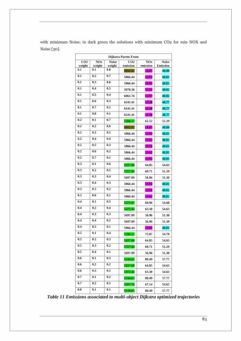
83

with minimum Noise; in dark green the solutions with minimum CO2 for min NOX and

Noise [30].

Dijkstra Pareto Front

CO2

weight

NOx

weight

Noise

weight

CO2

emission

NOx

emission

Noise

Emission

0.1 0.1 0.8 5812.52 54.87 48.80

0.1 0.2 0.7 5866.44 53.92 48.81

0.1 0.3 0.6 5866.44 53.92 48.81

0.1 0.4 0.5 5978.30 53.33 48.81

0.1 0.5 0.4 6061.76 52.97 48.82

0.1 0.6 0.3 6241.41 52.38 48.77

0.1 0.7 0.2 6241.41 52.38 48.77

0.1 0.8 0.1 6241.41 52.38 48.77

0.2 0.1 0.7 5506.27 62.52 51.29

0.2 0.2 0.6 5812.52 54.87 48.80

0.2 0.3 0.5 5866.44 53.92 48.81

0.2 0.4 0.4 5866.44 53.92 48.81

0.2 0.5 0.3 5866.44 53.92 48.81

0.2 0.6 0.2 5866.44 53.92 48.81

0.2 0.7 0.1 5866.44 53.92 48.81

0.3 0.1 0.6 5437.68 64.85 54.63

0.3 0.2 0.5 5557.44 60.71 51.29

0.3 0.3 0.4 5697.09 56.96 51.30

0.3 0.4 0.3 5866.44 53.92 48.81

0.3 0.5 0.2 5866.44 53.92 48.81

0.3 0.6 0.1 5866.44 53.92 48.81

0.4 0.1 0.5 5372.47 68.96 54.68

0.4 0.2 0.4 5472.44 63.30 54.63

0.4 0.3 0.3 5697.09 56.96 51.30

0.4 0.4 0.2 5697.09 56.96 51.30

0.4 0.5 0.1 5866.44 53.92 48.81

0.5 0.1 0.4 5296.21 75.87 54.70

0.5 0.2 0.3 5437.68 64.85 54.63

0.5 0.3 0.2 5557.44 60.71 51.29

0.5 0.4 0.1 5697.09 56.96 51.30

0.6 0.1 0.3 5244.65 80.49 57.77

0.6 0.2 0.2 5437.68 64.85 54.63

0.6 0.3 0.1 5472.44 63.30 54.63

0.7 0.1 0.2 5244.65 80.49 57.77

0.7 0.2 0.1 5397.78 67.14 54.65

0.8 0.1 0.1 5244.65 80.49 57.77

Table 11 Emissions associated to multi-object Dijkstra optimized trajectories

84

In the following table the 36 solutions found using Genetic algorithm are reported. The first

three columns report the weights used in the multi-objective function, the successive three

columns report the value of the three pollutants computed. In bold are reported the solutions

belonging to the Pareto front.

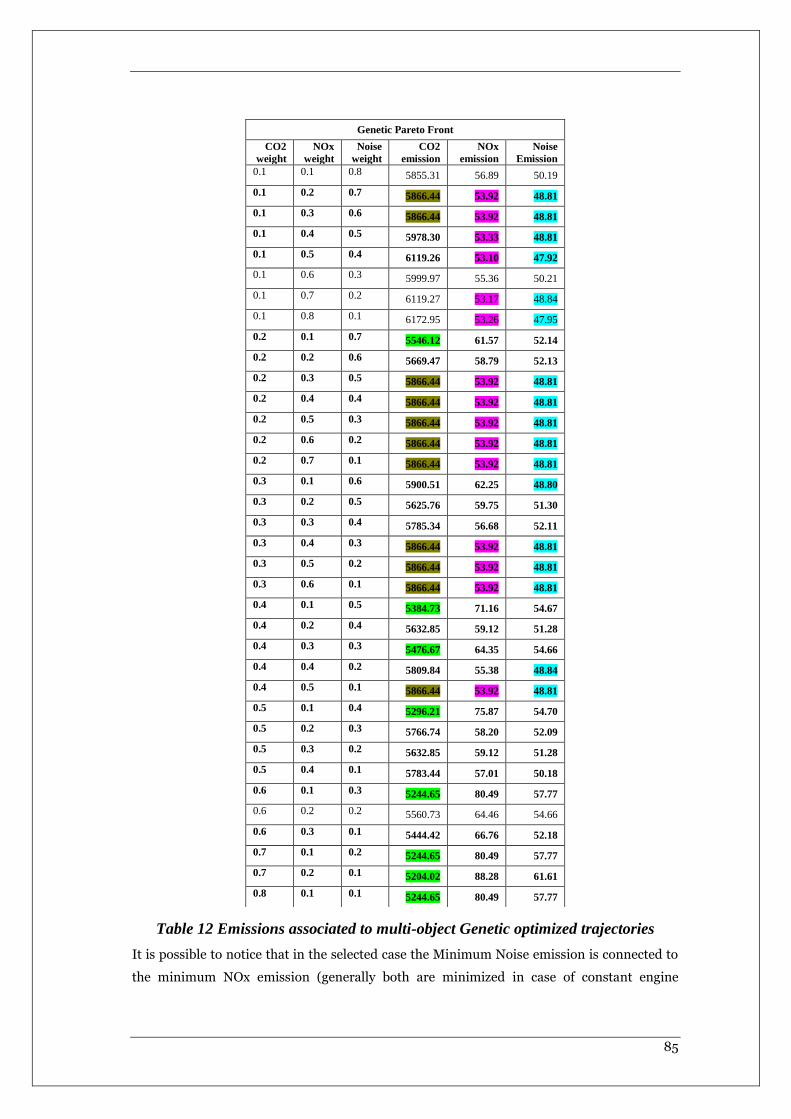
85

Table 12 Emissions associated to multi-object Genetic optimized trajectories

It is possible to notice that in the selected case the Minimum Noise emission is connected to

the minimum NOx emission (generally both are minimized in case of constant engine

Genetic Pareto Front

CO2

weight

NOx

weight

Noise

weight

CO2

emission

NOx

emission

Noise

Emission

0.1 0.1 0.8 5855.31 56.89 50.19

0.1 0.2 0.7 5866.44 53.92 48.81

0.1 0.3 0.6 5866.44 53.92 48.81

0.1 0.4 0.5 5978.30 53.33 48.81

0.1 0.5 0.4 6119.26 53.10 47.92

0.1 0.6 0.3 5999.97 55.36 50.21

0.1 0.7 0.2 6119.27 53.17 48.84

0.1 0.8 0.1 6172.95 53.26 47.95

0.2 0.1 0.7 5546.12 61.57 52.14

0.2 0.2 0.6 5669.47 58.79 52.13

0.2 0.3 0.5 5866.44 53.92 48.81

0.2 0.4 0.4 5866.44 53.92 48.81

0.2 0.5 0.3 5866.44 53.92 48.81

0.2 0.6 0.2 5866.44 53.92 48.81

0.2 0.7 0.1 5866.44 53.92 48.81

0.3 0.1 0.6 5900.51 62.25 48.80

0.3 0.2 0.5 5625.76 59.75 51.30

0.3 0.3 0.4 5785.34 56.68 52.11

0.3 0.4 0.3 5866.44 53.92 48.81

0.3 0.5 0.2 5866.44 53.92 48.81

0.3 0.6 0.1 5866.44 53.92 48.81

0.4 0.1 0.5 5384.73 71.16 54.67

0.4 0.2 0.4 5632.85 59.12 51.28

0.4 0.3 0.3 5476.67 64.35 54.66

0.4 0.4 0.2 5809.84 55.38 48.84

0.4 0.5 0.1 5866.44 53.92 48.81

0.5 0.1 0.4 5296.21 75.87 54.70

0.5 0.2 0.3 5766.74 58.20 52.09

0.5 0.3 0.2 5632.85 59.12 51.28

0.5 0.4 0.1 5783.44 57.01 50.18

0.6 0.1 0.3 5244.65 80.49 57.77

0.6 0.2 0.2 5560.73 64.46 54.66

0.6 0.3 0.1 5444.42 66.76 52.18

0.7 0.1 0.2 5244.65 80.49 57.77

0.7 0.2 0.1 5204.02 88.28 61.61

0.8 0.1 0.1 5244.65 80.49 57.77

86

regime). On the contrary Fuel consumption (and CO2 that is proportional by a factor of 3.18)

are minimized when NOx and Noise increase.

It is possible to identify some cases (underlined in dark green in table 4 and 5) in which there

is a limited emission of CO2 (fuel consumption) in correspondence of low emission of NOx

and Noise. Generally, the decision maker (i.e. the flight company) chooses the trajectory

emission index and the weights and the criteria to be used to optimize the trajectory.

6.4 Trajectory optimization with different weather

model and emissions weights

In the present paragraph, the results obtained applying, the described methods, to an A320,

in climb phase in real atmospheric condition, are presented. The considered trajectory is

originated from the International Airport of Fort Lauderdale-Hollywood (KFLL) on April 3rd

2013 at about 01 p.m. (UTC): NKS724. It is considered the climb phase, until cruise flight

level is reached. The aircraft is A320 and it is supposed that its mass is 64000 kg.

6.4.1 Meteorological data

Meteorological data are RAP data of April 3rd 2013 at about 01 p.m (UTC) (available in

http://motherlode.ucar.edu:8080/thredds/catalog/fmrc/NCEP/RAP/CONUS_20km/files/c

atalog.html). Wind speed and direction at altitude equal to about 5000 m are depicted in the

following figure (Fig. 27).

Fig.27 The Wind speed, direction (arrows) and intensity (more colors) at 5000 m

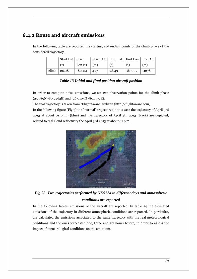
87

6.4.2 Route and aircraft emissions

In the following table are reported the starting and ending points of the climb phase of the

considered trajectory.

Table 13 Initial and final position aircraft position

In order to compute noise emissions, we set two observation points for the climb phase

(25.789N -80.2263E) and (26.0105N -80.1777E).

The real trajectory is taken from "FlightAware" website (http://flightaware.com).

In the following figure (Fig.3) the "normal" trajectory (in this case the trajectory of April 3rd

2013 at about 01 p.m.) (blue) and the trajectory of April 4th 2013 (black) are depicted,

related to real cloud reflectivity the April 3rd 2013 at about 01 p.m.

Fig.28 Two trajectories performed by NKS724 in different days and atmospheric

conditions are reported

In the following tables, emissions of the aircraft are reported. In table 14 the estimated

emissions of the trajectory in different atmospheric conditions are reported. In particular,

are calculated the emissions associated to the same trajectory with the real meteorological

conditions and the ones forecasted one, three and six hours before, in order to assess the

impact of meteorological conditions on the emissions.

Start Lat

(°)

Start

Lon (°)

Start Alt

(m)

End Lat

(°)

End Lon

(°)

End Alt

(m)

climb 26.08 -80.114 457 28.43 -81.009 11278

88

Table 14 estimated emissions of NKS724 in different atmospheric conditions

The differences in the calculated emissions depend mainly on wind and cloud reflectivity

values that are not so reliable for what concern the prediction [19]. On the other side,

pressure, temperature, and humidity prediction are more reliable in few hour prediction [19].

Then, using the weighted Graph of the feasible trajectories, the emissions associated to

different trajectories are calculated. In table 15 are reported the emissions associated to the

real flight (column 2 in table 3) and the ones associated to optimized trajectories, applying

Dijkstra mono or multi-object to select an optimized trajectory in accordance to different

criteria (table 3, in column 3 Dijkstra Mono-objective CO2, 4 Dijkstra Mono-objective NOx, 5

Dijkstra Multi-objective). The multi-objective trajectory optimization is calculated

attributing to NOx, CO2 and Noise emissions a weight of 0.4, 0.4, 0.2.

Table 15 NKS724 emissions and emission associated to optimized trajectories

6.4.3 Comparison of emissions associated to optimized

trajectory using Pareto

The optimization of more than one objective sets a problem on how to combine the single

objectives in order to find a satisfactory solution. In the reported tests the three pollutants

NKS724 Real

meteo

1 h

forecast

3 h

forecast

6 h

forecast

CO2 (kg) 5366 5415 5423 5407

NOx (kg) 62.99 63.76 63.98 63.63

Noise

(dB)

53.33 54.18 54.03 54.93

FA emit Dijkstra's algorithm

CO2 NOx MO2

CO2 (kg) 5366 5364 6249 5365

NOx (kg) 62,99 107 54,41 56

Noise (dB) 53.33 53,89 45,21 51.38

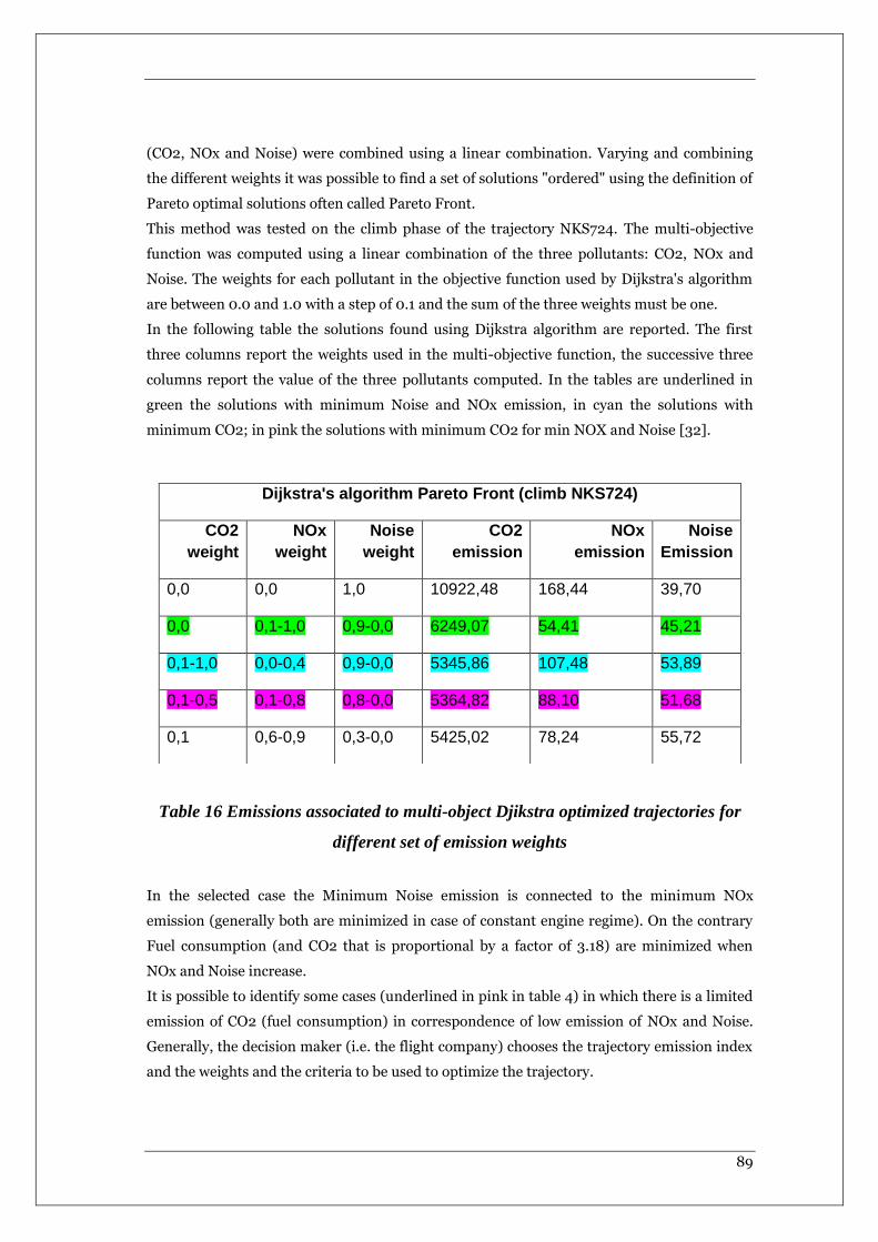
89

(CO2, NOx and Noise) were combined using a linear combination. Varying and combining

the different weights it was possible to find a set of solutions "ordered" using the definition of

Pareto optimal solutions often called Pareto Front.

This method was tested on the climb phase of the trajectory NKS724. The multi-objective

function was computed using a linear combination of the three pollutants: CO2, NOx and

Noise. The weights for each pollutant in the objective function used by Dijkstra's algorithm

are between 0.0 and 1.0 with a step of 0.1 and the sum of the three weights must be one.

In the following table the solutions found using Dijkstra algorithm are reported. The first

three columns report the weights used in the multi-objective function, the successive three

columns report the value of the three pollutants computed. In the tables are underlined in

green the solutions with minimum Noise and NOx emission, in cyan the solutions with

minimum CO2; in pink the solutions with minimum CO2 for min NOX and Noise [32].

Table 16 Emissions associated to multi-object Djikstra optimized trajectories for

different set of emission weights

In the selected case the Minimum Noise emission is connected to the minimum NOx

emission (generally both are minimized in case of constant engine regime). On the contrary

Fuel consumption (and CO2 that is proportional by a factor of 3.18) are minimized when

NOx and Noise increase.

It is possible to identify some cases (underlined in pink in table 4) in which there is a limited

emission of CO2 (fuel consumption) in correspondence of low emission of NOx and Noise.

Generally, the decision maker (i.e. the flight company) chooses the trajectory emission index

and the weights and the criteria to be used to optimize the trajectory.

Dijkstra's algorithm Pareto Front (climb NKS724)

CO2

weight

NOx

weight

Noise

weight

CO2

emission

NOx

emission

Noise

Emission

0,0 0,0 1,0 10922,48 168,44 39,70

0,0 0,1-1,0 0,9-0,0 6249,07 54,41 45,21

0,1-1,0 0,0-0,4 0,9-0,0 5345,86 107,48 53,89

0,1-0,5 0,1-0,8 0,8-0,0 5364,82 88,10 51,68

0,1 0,6-0,9 0,3-0,0 5425,02 78,24 55,72

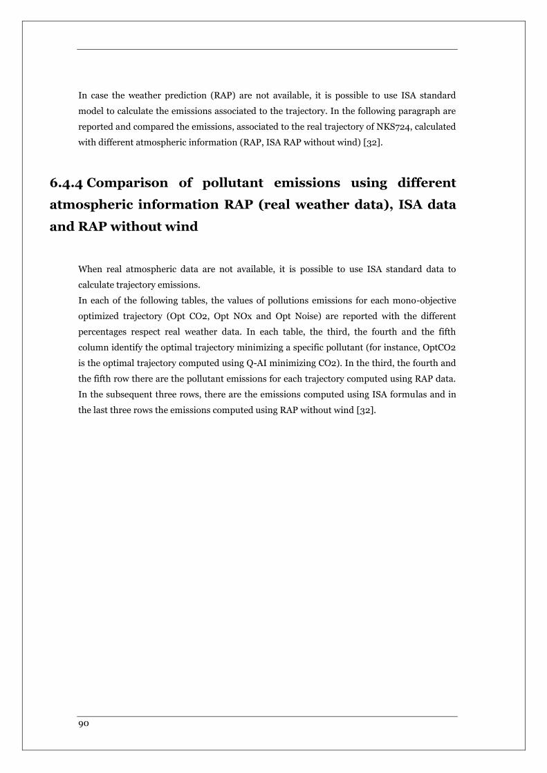
90

In case the weather prediction (RAP) are not available, it is possible to use ISA standard

model to calculate the emissions associated to the trajectory. In the following paragraph are

reported and compared the emissions, associated to the real trajectory of NKS724, calculated

with different atmospheric information (RAP, ISA RAP without wind) [32].

6.4.4 Comparison of pollutant emissions using different

atmospheric information RAP (real weather data), ISA data

and RAP without wind

When real atmospheric data are not available, it is possible to use ISA standard data to

calculate trajectory emissions.

In each of the following tables, the values of pollutions emissions for each mono-objective

optimized trajectory (Opt CO2, Opt NOx and Opt Noise) are reported with the different

percentages respect real weather data. In each table, the third, the fourth and the fifth

column identify the optimal trajectory minimizing a specific pollutant (for instance, OptCO2

is the optimal trajectory computed using Q-AI minimizing CO2). In the third, the fourth and

the fifth row there are the pollutant emissions for each trajectory computed using RAP data.

In the subsequent three rows, there are the emissions computed using ISA formulas and in

the last three rows the emissions computed using RAP without wind [32].

91

Table 17 Emissions associated to mono-object (CO2, NOx, Nose) optimized

trajectories calculated with real weather condition (from RAP), ISA standard

atmospheric condition and RAP data without wind

From the results, one can note that sometimes the optimal trajectory computed using RAP

data is not optimal if emissions are computed using ISA formulas or RAP without wind.

Moreover, the CO2 and NOx emissions computed using ISA formulas are less than the

emission computed using RAP data. On the contrary, the noise emissions are greater when

computed using ISA formulas. The emissions computed with ISA data and RAP without

wind are very similar. This proves that wind has a big impact on pollutant emissions.

6.5 Data validation in X-plane flight simulator

The optimized trajectories have been validated in a X-plane flight simulator (Fig. 3,4) in

which the correct models of A320 and engines were selected, the trajectories were uploaded

in the FMS (flight management system) and the real Grib file contained the considered RAP

NKS 724 Climb phase

Opt CO2 Opt NOx Opt Noise

RAP

CO2 (Kg) 5345 6249 10922

NOx (Kg) 107.47 54.4 168.4

Noise (dB) 53.8 45.2 39.6

ISA

CO2 (Kg) 5219 (-2%) 6066 (-2%) 7322 (-32%)

NOx (Kg) 87.8 (-18%) 51.1 (-6%) 85.7 (-49%)

Noise (dB) 72.5 (+25%) 59.9 (+24%) 57.9 (+31%)

RAP

without

wind

CO2 (Kg) 5234 (-2%) 6057 (-3%) 7330 (-32%)

NOx (Kg) 105.2 (-2%) 54 (-0,7%) 99.4 (-32%)

Noise (dB) 72.5 (+25%) 59.9 (+24%) 57.9 (+31%)

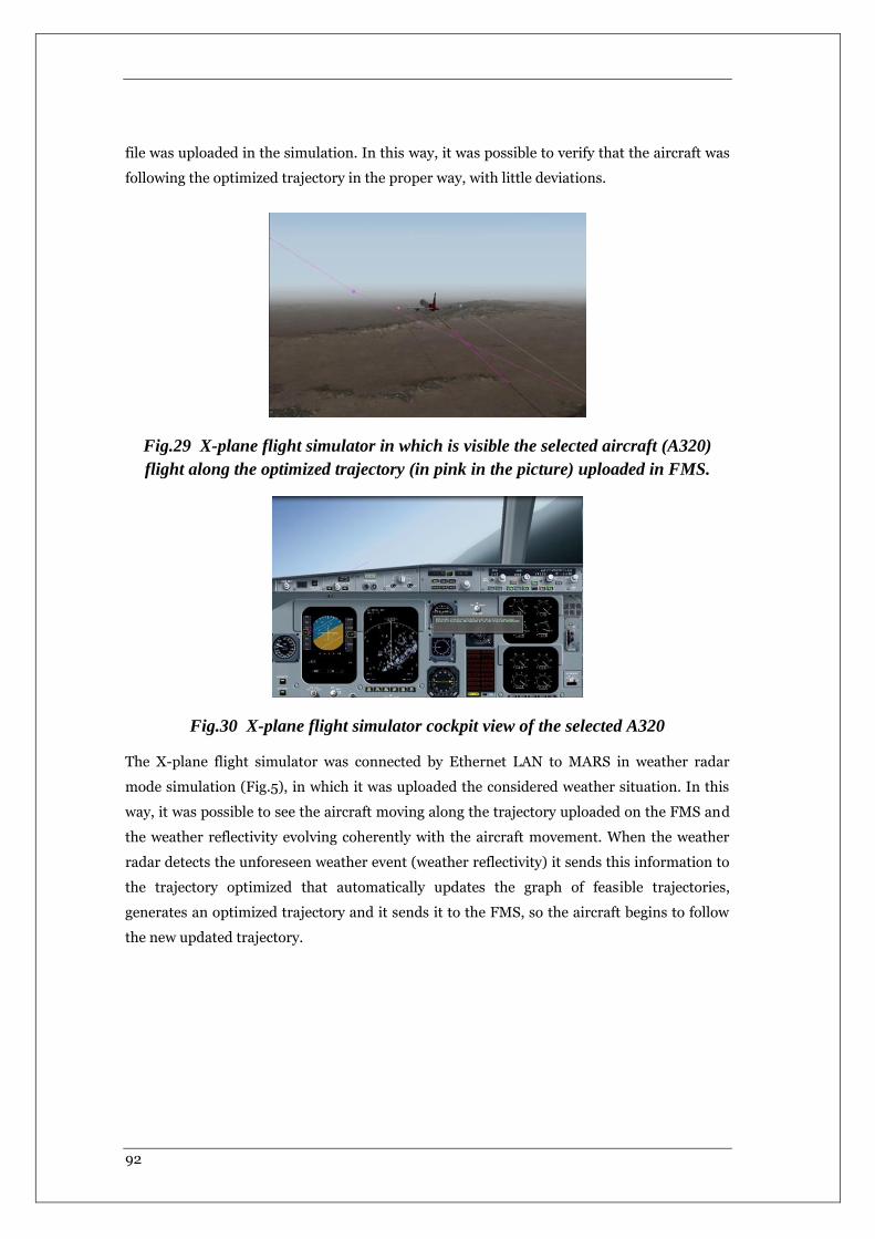
92

file was uploaded in the simulation. In this way, it was possible to verify that the aircraft was

following the optimized trajectory in the proper way, with little deviations.

Fig.29 X-plane flight simulator in which is visible the selected aircraft (A320)

flight along the optimized trajectory (in pink in the picture) uploaded in FMS.

Fig.30 X-plane flight simulator cockpit view of the selected A320

The X-plane flight simulator was connected by Ethernet LAN to MARS in weather radar

mode simulation (Fig.5), in which it was uploaded the considered weather situation. In this

way, it was possible to see the aircraft moving along the trajectory uploaded on the FMS and

the weather reflectivity evolving coherently with the aircraft movement. When the weather

radar detects the unforeseen weather event (weather reflectivity) it sends this information to

the trajectory optimized that automatically updates the graph of feasible trajectories,

generates an optimized trajectory and it sends it to the FMS, so the aircraft begins to follow

the new updated trajectory.

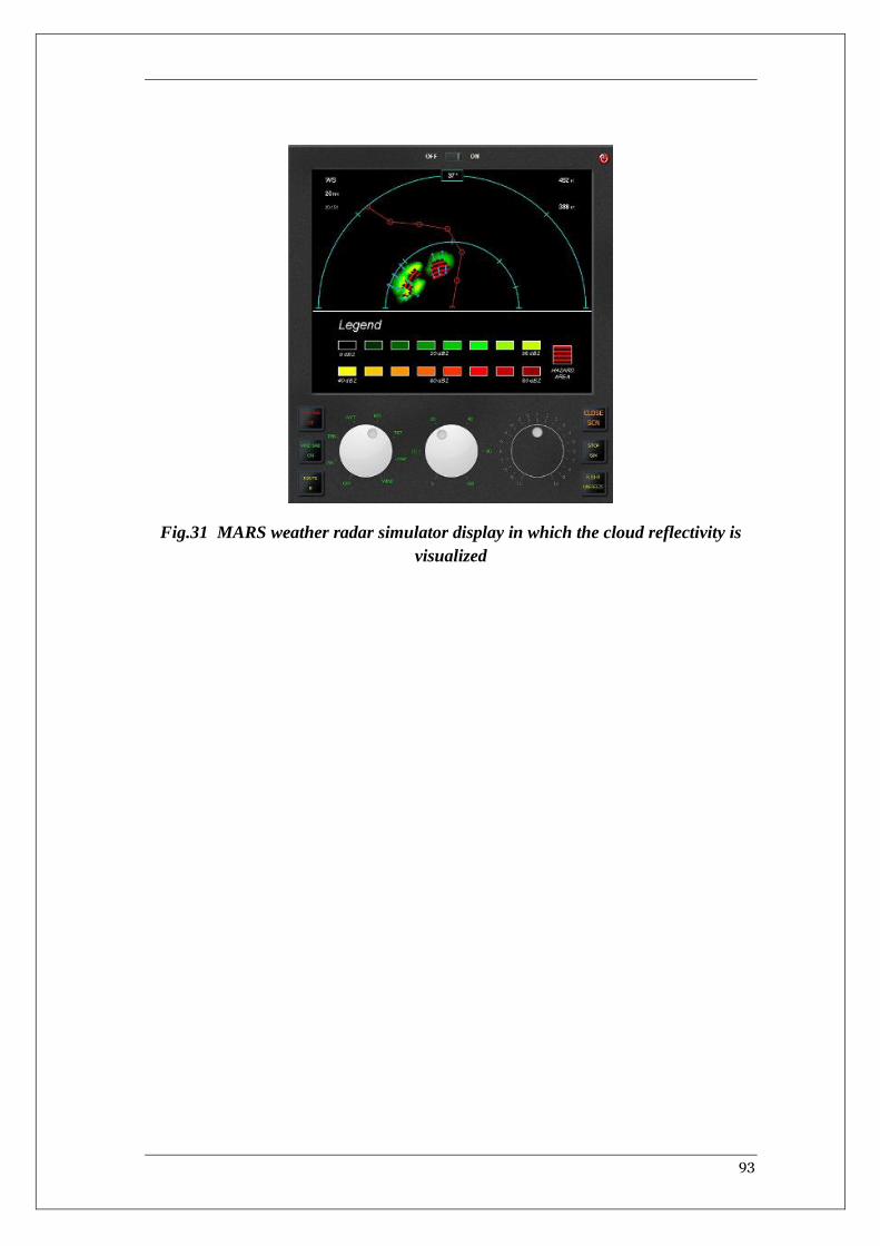
93

Fig.31 MARS weather radar simulator display in which the cloud reflectivity is

visualized

94

CHAPTER 7 MINIMUM

SIZE GRAPH

GENERATION AND

RESULTS

In this section is described our approach to automatically generate a minimum size graph of

trajectories to guarantee feasible acceptable solutions in a minimum computational time.

This approach is useful to run the trajectory optimizer on onboard computer that have

limited performances a process capacities. In the following paragraphs, will be detailed the

graph generation method and it will be underlined how the graph generation is different for

the different phases of flight. In particular, for the cruise phase are important the position

(latitude and longitude) variation while the altitude and speed variations are less important,

while in the climb and descent phase are more important the altitude and speed variations.

For the optimized trajectories, the climb and cruise phases are considered, because they are

the only ones in which it is possible to obtain a relevant decrease of fuel consumption and

emissions, while in descent phase generally the pilot perform a continuous descent approach

with the engine in idle mode, so there are no big margins of possible improvements.

7.1 Automatically Graph Generation

The construction procedure of the graph of feasible trajectories (base of data of our

optimizer) is the one described in par. 5.1.5. This procedure is automatized generating, in a

recursive way, graphs starting from very low resolution ones, that don’t provide feasible

95

solutions, and increasing the graph resolution till feasible solutions are available. So the

suggested method is based on recursive graphs generation that stops where suitable stop

criteria are reached. To optimize the graph generation process, these stops criteria, as it will

be shown later, is applied to a different DXi depending on the phase of flight.

In general, the chosen stop criteria of the graph generation are:

- DXi reached selected thresholds depending on the phase of flight;

- The fuel consumption doesn’t increase anymore for 3 consecutive steps

- The mean and mode of the maximum and minimum DXi (depending on phase of

flight) doesn’t increase for 3 consecutive steps.

To demonstrate the suggested procedure, several tests have been performed in Matlab. So,

several matlab programs have been implemented to automatically generate the minimum

graphs (for a selected accuracy) of the feasible trajectories for an A320 in climb and cruise

phase. The parameters automatically varied (till some stop criteria are reached) in such

matlab programs, are the minimum, maximum and step of 4 of the 5 parameters the

identified the nodes (latitude, longitude, altitude, and speed). The 5st parameter (heading

step) is fixed to 60° because we have a graph based on concentrated parameters, so each

waypoint identifies a different aircraft state.

7.2 Experimental set up

To demonstrate the proposed method, four use cases have been considered, in particular, 2

trajectories in cruise and 2 in climbs phase. Two of this use cases are identified the same

aircraft and trajectory considered in cap. 6, in particular, the test case 1 and the test case 2.

The method was successfully applied to the 4 use cases and the results are reported in the

following chapters.

7.2.1 Test cases characterization

In all the 4 cases the aircraft considered is an A320 and we suppose that during the flight the

mass of the aircraft is 64000 kg.

The flights are taken from real word (from flightaware) and the considered trajectories begin

and end the positions (considered state points) listed in the following table.

Initial states:

phase of flight

x0[degrees] y0[degrees] z0[m] Vtas0[m/s] heading0[degrees]

climb test3

40.86 -112.616 5882 197 260

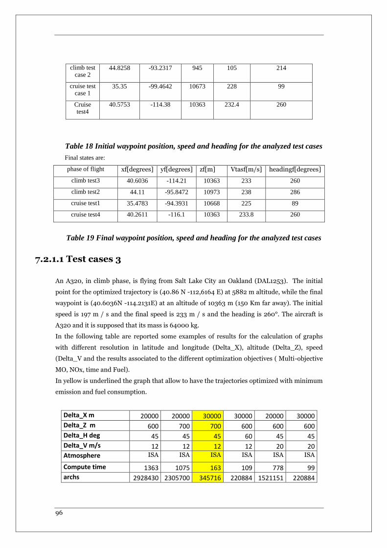
96

climb test case 2

44.8258 -93.2317 945 105 214

cruise test case 1

35.35 -99.4642 10673 228 99

Cruise test4

40.5753 -114.38 10363 232.4 260

Table 18 Initial waypoint position, speed and heading for the analyzed test cases

Final states are:

phase of flight xf[degrees] yf[degrees] zf[m] Vtasf[m/s] headingf[degrees]

climb test3 40.6036 -114.21 10363 233 260

climb test2 44.11 -95.8472 10973 238 286

cruise test1 35.4783 -94.3931 10668 225 89

cruise test4 40.2611 -116.1 10363 233.8 260

Table 19 Final waypoint position, speed and heading for the analyzed test cases

7.2.1.1 Test cases 3

An A320, in climb phase, is flying from Salt Lake City an Oakland (DAL1253). The initial

point for the optimized trajectory is (40.86 N -112,6164 E) at 5882 m altitude, while the final

waypoint is (40.6036N -114.2131E) at an altitude of 10363 m (150 Km far away). The initial

speed is 197 m / s and the final speed is 233 m / s and the heading is 260°. The aircraft is

A320 and it is supposed that its mass is 64000 kg.

In the following table are reported some examples of results for the calculation of graphs

with different resolution in latitude and longitude (Delta_X), altitude (Delta_Z), speed

(Delta_V and the results associated to the different optimization objectives ( Multi-objective

MO, NOx, time and Fuel).

In yellow is underlined the graph that allow to have the trajectories optimized with minimum

emission and fuel consumption.

Delta_X m 20000 20000 30000 30000 20000 30000

Delta_Z m 600 700 700 600 600 600

Delta_H deg 45 45 45 60 45 45

Delta_V m/s 12 12 12 12 20 20

Atmosphere ISA ISA ISA ISA ISA ISA

Compute time 1363 1075 163 109 778 99

archs 2928430 2305700 345716 220884 1521151 220884

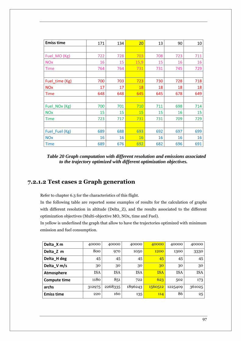
97

Emiss time 171 134 20 13 90 10

Fuel_MO (Kg) 722 728 703 708 723 711

NOx 16 15 15,9 15 16 16

Time 764 764 731 731 745 729

Fuel_time (Kg) 700 703 723 730 728 718

NOx 17 17 18 18 18 18

Time 648 648 645 645 678 649

Fuel_NOx (Kg) 700 701 710 711 698 714

NOx 15 15 15 15 16 15

Time 723 717 731 731 709 729

Fuel_Fuel (Kg) 689 688 693 692 697 699

NOx 16 16 16 16 16 16

Time 689 676 692 682 696 691

Table 20 Graph computation with different resolution and emissions associated to the trajectory optimized with different optimization objectives.

7.2.1.2 Test cases 2 Graph generation

Refer to chapter 6.3 for the characteristics of this flight.

In the following table are reported some examples of results for the calculation of graphs

with different resolution in altitude (Delta_Z), and the results associated to the different

optimization objectives (Multi-objective MO, NOx, time and Fuel).

In yellow is underlined the graph that allow to have the trajectories optimized with minimum

emission and fuel consumption.

Delta_X m 40000 40000 40000 40000 40000 40000

Delta_Z m 800 970 1050 1200 1300 3330

Delta_H deg 45 45 45 45 45 45

Delta_V m/s 30 30 30 30 30 30

Atmosphere ISA ISA ISA ISA ISA ISA

Compute time 1180 851 722 623 502 173

archs 312975 2268335 1896243 1560512 1225409 361025

Emiss time 220 160 135 114 86 25

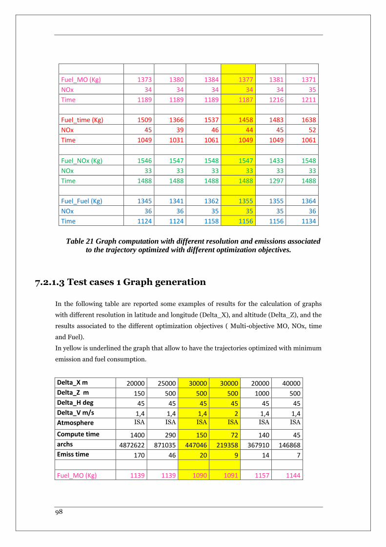
98

Fuel_MO (Kg) 1373 1380 1384 1377 1381 1371

NOx 34 34 34 34 34 35

Time 1189 1189 1189 1187 1216 1211

Fuel_time (Kg) 1509 1366 1537 1458 1483 1638

NOx 45 39 46 44 45 52

Time 1049 1031 1061 1049 1049 1061

Fuel_NOx (Kg) 1546 1547 1548 1547 1433 1548

NOx 33 33 33 33 33 33

Time 1488 1488 1488 1488 1297 1488

Fuel_Fuel (Kg) 1345 1341 1362 1355 1355 1364

NOx 36 36 35 35 35 36

Time 1124 1124 1158 1156 1156 1134

Table 21 Graph computation with different resolution and emissions associated to the trajectory optimized with different optimization objectives.

7.2.1.3 Test cases 1 Graph generation

In the following table are reported some examples of results for the calculation of graphs

with different resolution in latitude and longitude (Delta_X), and altitude (Delta_Z), and the

results associated to the different optimization objectives ( Multi-objective MO, NOx, time

and Fuel).

In yellow is underlined the graph that allow to have the trajectories optimized with minimum

emission and fuel consumption.

Delta_X m 20000 25000 30000 30000 20000 40000

Delta_Z m 150 500 500 500 1000 500

Delta_H deg 45 45 45 45 45 45

Delta_V m/s 1,4 1,4 1,4 2 1,4 1,4

Atmosphere ISA ISA ISA ISA ISA ISA

Compute time 1400 290 150 72 140 45

archs 4872622 871035 447046 219358 367910 146868

Emiss time 170 46 20 9 14 7

Fuel_MO (Kg) 1139 1139 1090 1091 1157 1144

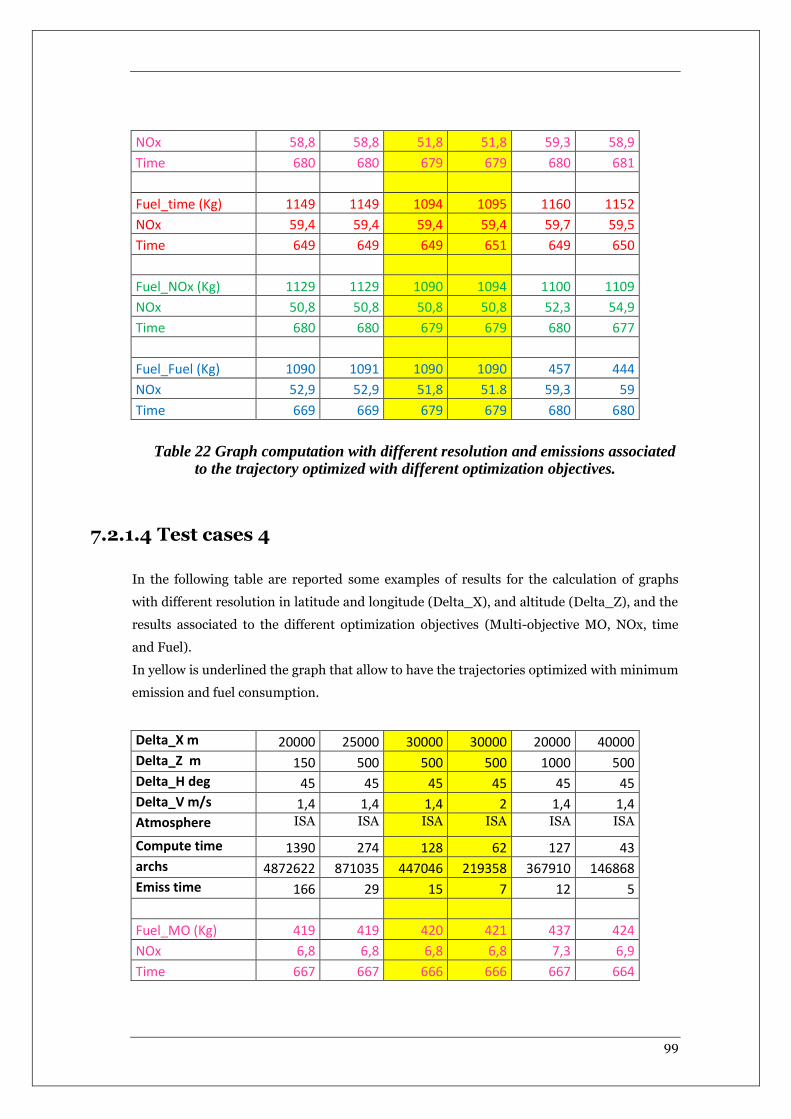
99

NOx 58,8 58,8 51,8 51,8 59,3 58,9

Time 680 680 679 679 680 681

Fuel_time (Kg) 1149 1149 1094 1095 1160 1152

NOx 59,4 59,4 59,4 59,4 59,7 59,5

Time 649 649 649 651 649 650

Fuel_NOx (Kg) 1129 1129 1090 1094 1100 1109

NOx 50,8 50,8 50,8 50,8 52,3 54,9

Time 680 680 679 679 680 677

Fuel_Fuel (Kg) 1090 1091 1090 1090 457 444

NOx 52,9 52,9 51,8 51.8 59,3 59

Time 669 669 679 679 680 680

Table 22 Graph computation with different resolution and emissions associated to the trajectory optimized with different optimization objectives.

7.2.1.4 Test cases 4

In the following table are reported some examples of results for the calculation of graphs

with different resolution in latitude and longitude (Delta_X), and altitude (Delta_Z), and the

results associated to the different optimization objectives (Multi-objective MO, NOx, time

and Fuel).

In yellow is underlined the graph that allow to have the trajectories optimized with minimum

emission and fuel consumption.

Delta_X m 20000 25000 30000 30000 20000 40000

Delta_Z m 150 500 500 500 1000 500

Delta_H deg 45 45 45 45 45 45

Delta_V m/s 1,4 1,4 1,4 2 1,4 1,4

Atmosphere ISA ISA ISA ISA ISA ISA

Compute time 1390 274 128 62 127 43

archs 4872622 871035 447046 219358 367910 146868

Emiss time 166 29 15 7 12 5

Fuel_MO (Kg) 419 419 420 421 437 424

NOx 6,8 6,8 6,8 6,8 7,3 6,9

Time 667 667 666 666 667 664

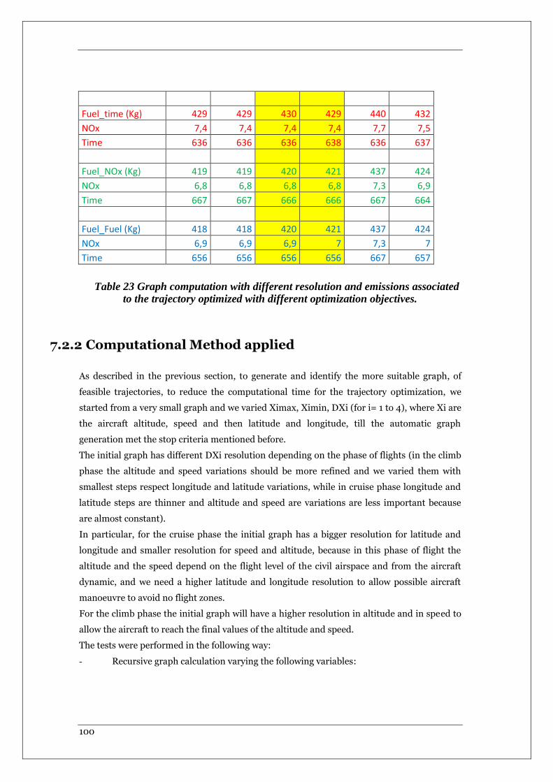
100

Fuel_time (Kg) 429 429 430 429 440 432

NOx 7,4 7,4 7,4 7,4 7,7 7,5

Time 636 636 636 638 636 637

Fuel_NOx (Kg) 419 419 420 421 437 424

NOx 6,8 6,8 6,8 6,8 7,3 6,9

Time 667 667 666 666 667 664

Fuel_Fuel (Kg) 418 418 420 421 437 424

NOx 6,9 6,9 6,9 7 7,3 7

Time 656 656 656 656 667 657

Table 23 Graph computation with different resolution and emissions associated to the trajectory optimized with different optimization objectives.

7.2.2 Computational Method applied

As described in the previous section, to generate and identify the more suitable graph, of

feasible trajectories, to reduce the computational time for the trajectory optimization, we

started from a very small graph and we varied Ximax, Ximin, DXi (for i= 1 to 4), where Xi are

the aircraft altitude, speed and then latitude and longitude, till the automatic graph

generation met the stop criteria mentioned before.

The initial graph has different DXi resolution depending on the phase of flights (in the climb

phase the altitude and speed variations should be more refined and we varied them with

smallest steps respect longitude and latitude variations, while in cruise phase longitude and

latitude steps are thinner and altitude and speed are variations are less important because

are almost constant).

In particular, for the cruise phase the initial graph has a bigger resolution for latitude and

longitude and smaller resolution for speed and altitude, because in this phase of flight the

altitude and the speed depend on the flight level of the civil airspace and from the aircraft

dynamic, and we need a higher latitude and longitude resolution to allow possible aircraft

manoeuvre to avoid no flight zones.

For the climb phase the initial graph will have a higher resolution in altitude and in speed to

allow the aircraft to reach the final values of the altitude and speed.

The tests were performed in the following way:

- Recursive graph calculation varying the following variables:

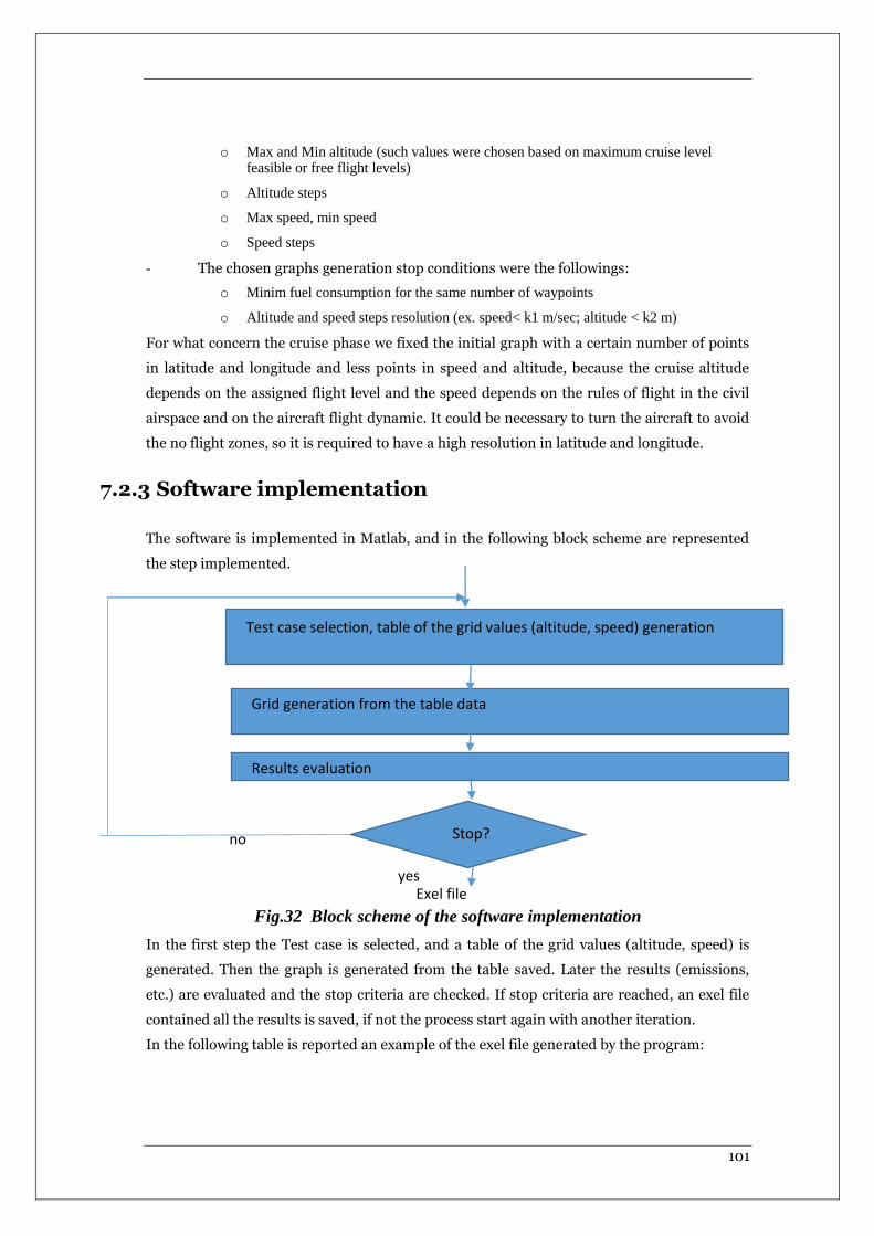
101

o Max and Min altitude (such values were chosen based on maximum cruise level feasible or free flight levels)

o Altitude steps

o Max speed, min speed

o Speed steps

- The chosen graphs generation stop conditions were the followings:

o Minim fuel consumption for the same number of waypoints

o Altitude and speed steps resolution (ex. speed< k1 m/sec; altitude < k2 m)

For what concern the cruise phase we fixed the initial graph with a certain number of points

in latitude and longitude and less points in speed and altitude, because the cruise altitude

depends on the assigned flight level and the speed depends on the rules of flight in the civil

airspace and on the aircraft flight dynamic. It could be necessary to turn the aircraft to avoid

the no flight zones, so it is required to have a high resolution in latitude and longitude.

7.2.3 Software implementation

The software is implemented in Matlab, and in the following block scheme are represented

the step implemented.

Fig.32 Block scheme of the software implementation

In the first step the Test case is selected, and a table of the grid values (altitude, speed) is

generated. Then the graph is generated from the table saved. Later the results (emissions,

etc.) are evaluated and the stop criteria are checked. If stop criteria are reached, an exel file

contained all the results is saved, if not the process start again with another iteration.

In the following table is reported an example of the exel file generated by the program:

Test case selection, table of the grid values (altitude, speed) generation

Grid generation from the table data

Results evaluation

Stop? no

yes Exel file

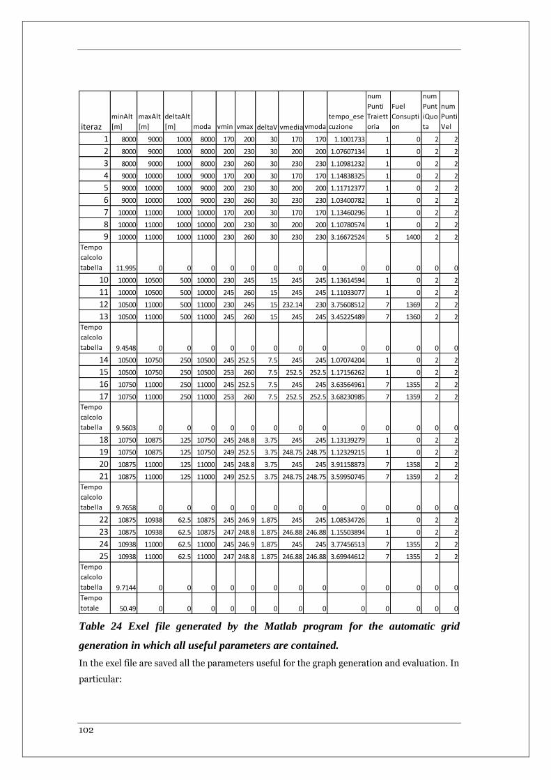
102

iterazminAlt

[m]

maxAlt

[m]

deltaAlt

[m] moda vmin vmax deltaV vmedia vmoda

tempo_ese

cuzione

num

Punti

Traiett

oria

Fuel

Consupti

on

num

Punt

iQuo

ta

num

Punti

Vel

1 8000 9000 1000 8000 170 200 30 170 170 1.1001733 1 0 2 2

2 8000 9000 1000 8000 200 230 30 200 200 1.07607134 1 0 2 2

3 8000 9000 1000 8000 230 260 30 230 230 1.10981232 1 0 2 2

4 9000 10000 1000 9000 170 200 30 170 170 1.14838325 1 0 2 2

5 9000 10000 1000 9000 200 230 30 200 200 1.11712377 1 0 2 2

6 9000 10000 1000 9000 230 260 30 230 230 1.03400782 1 0 2 2

7 10000 11000 1000 10000 170 200 30 170 170 1.13460296 1 0 2 2

8 10000 11000 1000 10000 200 230 30 200 200 1.10780574 1 0 2 2

9 10000 11000 1000 11000 230 260 30 230 230 3.16672524 5 1400 2 2

Tempo

calcolo

tabella 11.995 0 0 0 0 0 0 0 0 0 0 0 0 0

10 10000 10500 500 10000 230 245 15 245 245 1.13614594 1 0 2 2

11 10000 10500 500 10000 245 260 15 245 245 1.11033077 1 0 2 2

12 10500 11000 500 11000 230 245 15 232.14 230 3.75608512 7 1369 2 2

13 10500 11000 500 11000 245 260 15 245 245 3.45225489 7 1360 2 2

Tempo

calcolo

tabella 9.4548 0 0 0 0 0 0 0 0 0 0 0 0 0

14 10500 10750 250 10500 245 252.5 7.5 245 245 1.07074204 1 0 2 2

15 10500 10750 250 10500 253 260 7.5 252.5 252.5 1.17156262 1 0 2 2

16 10750 11000 250 11000 245 252.5 7.5 245 245 3.63564961 7 1355 2 2

17 10750 11000 250 11000 253 260 7.5 252.5 252.5 3.68230985 7 1359 2 2

Tempo

calcolo

tabella 9.5603 0 0 0 0 0 0 0 0 0 0 0 0 0

18 10750 10875 125 10750 245 248.8 3.75 245 245 1.13139279 1 0 2 2

19 10750 10875 125 10750 249 252.5 3.75 248.75 248.75 1.12329215 1 0 2 2

20 10875 11000 125 11000 245 248.8 3.75 245 245 3.91158873 7 1358 2 2

21 10875 11000 125 11000 249 252.5 3.75 248.75 248.75 3.59950745 7 1359 2 2

Tempo

calcolo

tabella 9.7658 0 0 0 0 0 0 0 0 0 0 0 0 0

22 10875 10938 62.5 10875 245 246.9 1.875 245 245 1.08534726 1 0 2 2

23 10875 10938 62.5 10875 247 248.8 1.875 246.88 246.88 1.15503894 1 0 2 2

24 10938 11000 62.5 11000 245 246.9 1.875 245 245 3.77456513 7 1355 2 2

25 10938 11000 62.5 11000 247 248.8 1.875 246.88 246.88 3.69944612 7 1355 2 2

Tempo

calcolo

tabella 9.7144 0 0 0 0 0 0 0 0 0 0 0 0 0

Tempo

totale 50.49 0 0 0 0 0 0 0 0 0 0 0 0 0

Table 24 Exel file generated by the Matlab program for the automatic grid

generation in which all useful parameters are contained.

In the exel file are saved all the parameters useful for the graph generation and evaluation. In

particular:

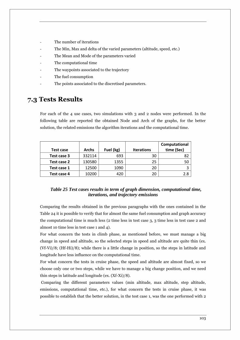
103

- The number of iterations

- The Min, Max and delta of the varied parameters (altitude, speed, etc.)

- The Mean and Mode of the parameters varied

- The computational time

- The waypoints associated to the trajectory

- The fuel consumption

- The points associated to the discretised parameters.

7.3 Tests Results

For each of the 4 use cases, two simulations with 3 and 2 nodes were performed. In the

following table are reported the obtained Node and Arch of the graphs, for the better

solution, the related emissions the algorithm iterations and the computational time.

Test case Archs Fuel (kg) Iterations Computational

time (Sec)

Test case 3 332114 693 30 82

Test case 2 130580 1355 25 50

Test case 1 12500 1090 20 3

Test case 4 10200 420 20 2.8

Table 25 Test cases results in term of graph dimension, computational time, iterations, and trajectory emissions

Comparing the results obtained in the previous paragraphs with the ones contained in the

Table 24 it is possible to verify that for almost the same fuel consumption and graph accuracy

the computational time is much less (2 time less in test case 3, 3 time less in test case 2 and

almost 10 time less in test case 1 and 4).

For what concern the tests in climb phase, as mentioned before, we must manage a big

change in speed and altitude, so the selected steps in speed and altitude are quite thin (ex.

(Vf-Vi)/8; (Hf-Hi)/8); while there is a little change in position, so the steps in latitude and

longitude have less influence on the computational time.

For what concern the tests in cruise phase, the speed and altitude are almost fixed, so we

choose only one or two steps, while we have to manage a big change position, and we need

thin steps in latitude and longitude (ex. (Xf-Xi)/8).

Comparing the different parameters values (min altitude, max altitude, step altitude,

emissions, computational time, etc.), for what concern the tests in cruise phase, it was

possible to establish that the better solution, in the test case 1, was the one performed with 2

104

nodes simulation since all the parameters values were the same for the minimum

computational time. In the test 4 use case the results are almost the same for 2 and 3 nodes,

and the computational time is very low in both cases. For what concern the tests in climb

phase, to reach a suitable solution, and obtain a graph able to cover all the foreseen range in

altitude and speed, are required more nodes, interactions, and computational time.

The previous calculation where performed in a portable workstation with the following

characteristics:

- Operating System: Genuine Windows 7 Professional 64

- Processor: 3rd Generation Intel® CoreTM i7 Quad-Core1

- Memory: DDR3 SDRAM PC3-12800, 1600 MHz, dual-core processors support 2

memory slots, 2/4/8 GB16 SODIMMs

- Internal Storage: 320/500/750 GB 7200 rpm HDD, 500 GB 7200 rpm SED (Self

Encrypting Drive), SATA 6 Gb/s, 128/180 GB SSD

- Graphics: NVIDIA Quadro K2000M, with 2 GB dedicated DDR3 video memory

For the considered test cases, the computational time is suitable for on-board application,

since the available time is around 5 minutes and the obtained computational time is less than

50 seconds. The proposed method allows to generate an adaptive grid in the minimum time

with a low dimension for the required accuracy. These graphs have been compared with big

graphs, in terms on emissions, graph dimension, arches, computational time. These graphs

allow minimum memory/space occupancy and minimum computational time.

When the computational time is not acceptable for on-board applications, other graph

generation strategies should be applied, like to generate set of smaller graphs connected

together in the interested space. That would drastically decrease the computational times

and allow an on-board real time trajectory optimization.

105

CHAPTER 8

CONCLUSIONS

In the present thesis, important problems for the aircraft flight have been taken into account

and the possible solutions have been proposed. The problems described are the necessity for

the aircraft to avoid bad weather conditions and to the reduce the fuel consumption and the

pullant emissions. The proposed solution is a graph based on-board multi-object trajectory

optimizer.

In the first part of this thesis is provide an overview of the weather phenomenon dangerous

for the aircraft flight and an overview of avionic instruments and information sources that

can provide weather information to the pilot. Then an overview on civil aircraft flight in

terms of aircraft categories, performed trajectory and phase of flight is provided to

contextualize the object of the proposed optimization (aircraft trajectory for different phases

of flight). Later an overview of the available trajectory optimization algorithms and methods

is provided and some performance comparison is described. The next chapter report the

description of our approach for the multi-object aircraft trajectory optimization for weather

avoidance and emission reduction. The algorithm proposed is Dijkstra for the generation of

the graph of feasible trajectories in a certain volume of space. Such graph is valid for a certain

aircraft of which is available the performance model, in a certain airspace volume, in which

are available the atmospheric conditions. For this reason, are taken into account and

described the model used to generate the graph, in particular the aircraft, emission, weather

and engine models. In the next chapter, some results for a typical civil aircraft (A320) are

provided and the fuel consumption of the optimized trajectories are compared with the real

trajectory performed by the aircraft and downloaded from “flightaware” database. The

obtained results are quite interested because show a significant fuel and emission reduction

possibility, while avoiding bad weather conditions, respect the real flight. In this chapter is

also shown how much unreliable are the weather predictions, in particular, the weather

106

reflectivity and the wind, and that justify why an on-board trajectory optimizer would be very

useful. Unfortunately, on-board there are avionic devices with limits in performances and in

computational time. For this reason, finally it is proposed an innovative method to

automatically generate a graph of trajectories (to be used as base of data for the trajectory

optimizer), with minimum size and computational time suitable for on-board applications,

and some interesting result is provided. The proposed method identifies a process to

automatically generate the better graphs, for the trajectory optimizer, in terms minimal

dimension and computational time, so suitable for on-board application integrated in a

decisional support system. The possible on-board devices target for such a decision support

system are EFB (Electronic Flight Bag) or tablet.

107

Acronyms

AAC Airline Administrative Control

ACARE Advisory Council for Aeronautics Research in Europe

ACARS Aircraft Communications and Reporting System

AOC Aircraft Operational Control

ATC Air Traffic Control

A-WXR Advanced Weather Radar

dB DeciBel

BADA Base of Aircraft DAta

CAT clear air turbulence

deg degree(s)

DO DOcument

DOW Description Of Work

DSS Decision Support System

EEC Eurocontrol Experimental Centre

EFB Electronic Flight Bag

FAA Federal Aviation Administration

FMS Flight Management System

GRIB Gridded Binary Data files (General Regularly-distributed Information in Binary form)

GRUMP Global Rural-Urban Mapping Project,

ICAO International Civil Aviation Organization

ICD Interface Control Document

ID IDentification

ISA International Standard Atmosphere

ITD Integrated Technology Demonstrator

JTI Joint Technology Initiative

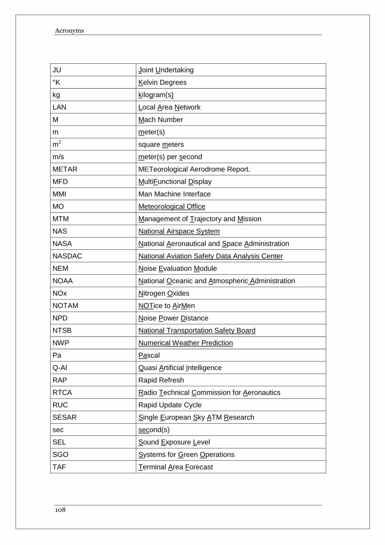
Acronyms

108

JU Joint Undertaking

°K Kelvin Degrees

kg kilogram(s)

LAN Local Area Network

M Mach Number

m meter(s)

m2 square meters

m/s meter(s) per second

METAR METeorological Aerodrome Report.

MFD MultiFunctional Display

MMI Man Machine Interface

MO Meteorological Office

MTM Management of Trajectory and Mission

NAS National Airspace System

NASA National Aeronautical and Space Administration

NASDAC National Aviation Safety Data Analysis Center

NEM Noise Evaluation Module

NOAA National Oceanic and Atmospheric Administration

NOx Nitrogen Oxides

NOTAM NOTice to AirMen

NPD Noise Power Distance

NTSB National Transportation Safety Board

NWP Numerical Weather Prediction

Pa Pascal

Q-AI Quasi Artificial Intelligence

RAP Rapid Refresh

RTCA Radio Technical Commission for Aeronautics

RUC Rapid Update Cycle

SESAR Single European Sky ATM Research

sec second(s)

SEL Sound Exposure Level

SGO Systems for Green Operations

TAF Terminal Area Forecast

109

TM Trajectory Management

UDP User Datagram Protocol

WAFC World Area Forecast Centres

WP Work Package

WXR Weather Radar

Acronyms

110

References

[1] ACARE, European Aeronautics – A Vision for 2020 – Report of the Group of Personalities,

January 2001

[2] ACARE, Strategic Research Agenda 1, October 2002

[3] ACARE, Strategic Research Agenda 2, October 2004

[4] D. Michalek and H. Balakrishnan, Identification of Robust Routes using Convective Weather

Forecasts, 8th USA/Europe Air Traffic Management R&D Seminar, Napa Valley, CA, June/July

2009.

[5] M. Rubnich and R. DeLaura, An Algorithm to Identify Robust Convective Weather Avoidance

Polygons in En Route Airspace, AIAA Aviation Technology, Integration, and Operations (ATIO)

Conference 13 - 15 September 2010, Fort Worth, Texas.

[6] M.H. Nguyen, S. Alam, J. Tang, and H. Abbass, Ants-inspired dynamic weather avoidance

trajectories in a traffic constrained enroute airspace; 6th EUROCONTROL Innovative Research

Workshop & Exhibition,12- 2007, pp. 205–212.

[7] The Potential Impacts of Climate Change on Transportation- Gloria Kelusa

[8] Climatology manual for Airline Pilots – H.R. Quantick FRAeS, FRMetS

[9] Panel on Atmospheric Effects of Aviation and Board on Atmospheric Sciences & Climate and

Commission on Geosciences & Environment & Resources and National Research Council,

Atmospheric Effects of Aviation: A Review of NASA’s Subsonic Assessment Project, 1999

[10] WMO Publication No: 306, Manual on Codes, Volume 1.2, Part B – Binary Codes

[11] http://nomads.ncdc.noaa.gov

[12] Oxford Aviation Training, Jeppesen, (2002), "JAA Airline Transport Pilot's Licence, Theoretical

Knowledge Manual, 022 INSTRUMENTATION" Second Edition, First Impression, Osford

Aviation Services Limitet 2001, England.

[13] Oxford Aviation Training, Jeppesen, (2002), "JAA Airline Transport Pilot's Licence, Theoretical

Knowledge Manual, 050 METEREOLOGY" Second Edition, First Impression, Osford Aviation

Services Limitet 2001, England.

[14] Colella G., (2009), "Meteorologia Aeronautica", V Ed., IBN Editore, Roma

[15] Trebbi R., (2012), "Meteorologia per Piloti", Aviabooks Editore (La Bancarele Aeronautica),

Milano

[16] Moir I., Seabridge A., (2008), "Aircraft System", Third Edition John, Wiley & Sons Ltd.,

England, Pag. 441-493

[17] Diston D.J., (University of Manchester), (2009), "Computational Modelling and Simulation of

Aircraft and the Environment", First Edition John, Wiley & Sons Ltd., England.

[18] Yiyuan Zhao and Rhonda a. Slattery. Capture conditions for merging trajectory segments to

model realistic aircraft descents. Journal of Guidance, Control, and Dynamics, 19(2):453{460,

March 1996.

[19] G. Serafino, M. Bernabò, S. Mininel, G. Stecco, M. Nolich, W. Ukovich, G. Pedroncelli, M. P.

Fanti, "Effects of weather condition on aircraft emissions in climb phase", Digital Avionics

Systems Conference (DASC), Williamsburg, VA, USA, pp. 3A6-1 - 3A6-12, October 2012.

[20] Baughcum, S.L., T. G. Tritz, S. C. Henderson, D. C. Pickett, 1996, Scheduled Civil Aircraft

Emissions Inventories for 1992: Database Development and Analysis, Appendix D: Boeing

Method 2 Fuel Flow Methodology Description, Report NASA CR 4700, The Boeing Company

[21] Nuic, A., 2012, User Manual for the base of AircraftData (BADA) Revision 3.10, Eurocontrol

111

[22] Experimental Center.International Civil Aviation Organization (ICAO). ICAO Engine Exhaust

Emissions Databank, Issue 15-B, 2007.

[23] EUROCONTROL Experimental Center, The Advanced Emission Model (AEM3) Version 1.5 –

Validation Report; EEC/SEE/2004/004

[24] Airbus A-320 POH: Pilot's Operating Handbook", http://www.despair.ch/staff/library/thc003.pdf

[25] AIRBUS, "A318/A319/A320/A321 Flight deck and systems briefing for pilots", Ref. STL

945.7136/97 – Issue 4, 2007

[26] M.P. Fanti, S. Mininel, M. Nolich, G. Stecco, W. Ukovich, M. Bernabò and G. Serafino, Flight

Path Optimization for Minimizing Emissions and Avoiding Weather Hazard, ACC, 06/2014

[27] ICAO, ICAO Engine Exhaust Emissions Databank, Issue 15-B, 2007.

[28] ICAO, “Environmental report 2010,” 2010.

[29] R. K. Ahuja, T. L. Magnanti, and J. B. Orlin. Network flows: Theory, Algorithms, and

Applications. Prentice-Hall, NJ, 1993

[30] G. SERAFINO, MULTI-OBJECTIVE TRAJECTORY OPTIMIZATION TO REDUCE

AIRCRAFT EMISSIONS IN CASE OF UNFORESEEN WEATHER EVENTS, 29TH ICAS

2014 CONFERENCE, ST. PETERSBURG, 7-12 SEPTEMBER 2014

[31] ECAC.CEAC Doc 29, Report on Standard Method of Computing Noise Contours around Civil

Airports,Volume 1: Application guide, 2005.

[32] EFFECTS OF WEATHER CONDITION ON AIRCRAFT EMISSION IN CLIMB PHASE,

MESAS 2015 CONGRESS, PRAGUE, 29-30 APRIL 2015, G. SERAFINO, Springer

[33] G. SERAFINO, ONBOARD TRAJECTORY OPTIMIZATION FOR WEATHER AVOIDANCE

AND EMISSION REDUCTION, GREENER AVIATION, 3AF, BRUXELLES, 11-13

OCTOBER 2016

[34] David H. Jacobson, David Q. Mayne. "Differential Dynamic Programming" Elsevier, 1970.

[35] Patterson, Michael A.; Rao, Anil V. (2014-10-01). "GPOPS-II: A MATLAB Software for

Solving Multiple-Phase Optimal Control Problems Using hp-Adaptive Gaussian Quadrature

Collocation Methods and Sparse Nonlinear Programming". ACM Trans. Math. Softw. 41 (1):

1:1–1:37. doi:10.1145/2558904. ISSN 0098-3500.

[36] Waitz, I., J. Townsend, J. Cutcher-Gershenfeld, E. Greitzer, J. Kerrebrock, 2004, Aviation and

the environment: Report to the United States Congress, Partnership for Air Transp. Noise and

Emissions Reduction, MIT, Cambridge.

[37] Nuic, A., 2012, User Manual for the base of Aircraft Data (BADA) Revision 3.10, Eurocontrol

Experimental Center.

[38] Dopelheuer, A.,2000, Aircraft emission parameter modeling, Air & Space Europe, 2, 34-37.

[39] International Civil Aviation Organization (ICAO). ICAO Engine Exhaust Emissions Databank,

Issue 15-B, 2007.

[40] Baughcum, S.L., T. G. Tritz, S. C. Henderson, D. C. Pickett, 1996, Scheduled Civil Aircraft

Emissions Inventories for 1992: Database Development and Analysis, Appendix D: Boeing

Method 2 Fuel Flow Methodology Description, Report NASA CR 4700, The Boeing Company.

[41] International Civil Aviation Organization (ICAO). ICAO Engine Exhaust Emissions Databank,

Issue 15-B, 2007

[42] The Advanced Emission Model (AEMIII),ver 1.5, Eurocontrol, Validation report, 2004

[43] ECAC.CEAC Doc 29 , Report on Standard Method of Computing Noise Contours around Civil

Airports, Volume 1: Application guide, 2005.

[44] Dopelheuer, A.,2000,Aircraft emission parameter modeling, Air & Space Europe, 2, 34-37.

[45] International Electrotechnical Commission: Sound level meters. IEC 61672-1 (2002)

[46] International Organization for Standardization: Acoustics – Procedure for describing aircraft

noise heard on the ground. ISO 3891 (1978). [This standard may be replaced or supplemented by

a new standard that is currently in draft form as ISO/CD 20906 (2003): Unattended monitoring of

aircraft sound in the vicinity of airports.]

[47] International Organization for Standardization: Acoustics – Description, measurement and

assessment of environmental noise – Part 1: Basic quantities and assessment procedures. ISO

1996-1 (2001).

[48] International Civil Aviation Organization: International Standards and Recommended Practices,

Environmental Protection, Annex 16, Volume I, Aircraft Noise, 4th Edition, July 2005.

Acronyms

112

[49] Eric Homan, Peter Martin, Thomas P• utz, Aymeric Trzmiel, and Karim Zeghal. Airborne

Spacing: Flight Deck View of Compatibility with Continuous Descent Approach (CDA).

Interface, 2007.

[50] G.L. Slater. Study on variations in vertical profile for CDA descents - aiaa-2007-7778, 2009. [9th

AIAA Aviation Technology, Integration, and Operations Conference 21 - 23 September 2009].

[51] John E. Robinson III Keenan Roach. A Terminal Area Analysis of Continuous Ascent Departure

Fuel Use at Dallas/Fort Worth International Airport – aiaa, 2010. [10th AIAA Aviation

Technology, Integration, and Operations (ATIO) Conference 13 - 15 September 2010, Fort

Worth, Texas].

[52] Francois Le Sellier. Discrete Real-Time Flight Plan Optimization. 1999.

[53] W.a. Kamal and I. Postlethwaite. Real Time Trajectory Planning for UAVs

[54] Using MILP. Proceedings of the 44th IEEE Conference on Decision and Control, 2005.

[55] I. M. Ross and M. Karpenko, "A Review of Pseudospectral Optimal Control: From Theory to

Flight," Annual Reviews in Control, Vol. 36, pp. 182-197, 2012.

[56] Survey of Numerical Methods for Trajectory Optimization; John T. Betts Journal of Guidance,

Control, and Dynamics 1998; 0731-5090 vol.21 no.2 (193-207)

[57] Francois Le Sellier. Discrete Real-Time Flight Plan Optimization. 1999.

[58] W.a. Kamal and I. Postlethwaite. Real Time Trajectory Planning for UAVs

[59] Using MILP. Proceedings of the 44th IEEE Conference on Decision and Control, 2005.

[60] Arthur Richards and Jonathan P How. Collision Avoidance Using Mixed Integer Linear

Programming Hong Yang and Yiyuan Zhao. Trajectory Planning for Autonomous Aerospace

Vehicles amid Known Obstacles and Conflicts. Journal of Guidance, Control, and Dynamics,

November 2004.

[61] John T. Betts "Practical Methods for Optimal Control and Estimation Using Nonlinear

Programming" SIAM Advances in Design and Control, 2010.

[62] Christopher L. Darby, William W. Hager, and Anil V. Rao. "An hp-adaptive pseudospectral

method for solving optimal control problems." Optimal Control Applications and Methods, 2010.

[63] Patterson, Michael A.; Rao, Anil V. (2014-10-01). "GPOPS-II: A MATLAB Software for

Solving Multiple-Phase Optimal Control Problems Using hp-Adaptive Gaussian Quadrature

Collocation Methods and Sparse Nonlinear Programming". ACM Trans. Math. Softw. 41 (1):

1:1–1:37. doi:10.1145/2558904. ISSN 0098-3500.

[64] I. M. Ross and M. Karpenko, "A Review of Pseudospectral Optimal Control: From Theory to

Flight," Annual Reviews in Control, Vol. 36, pp. 182-197, 2012.

[65] Survey of Numerical Methods for Trajectory Optimization; John T. Betts Journal of Guidance,

Control, and Dynamics 1998; 0731-5090 vol.21 no.2 (193-207)

[66] Anil V. Rao "A survey of numerical methods for optimal control" Advances in Astronautical

Sciences, 2009.

[67] Camila C. Francolin, David A. Benson, William W. Hager, Anil V. Rao. "Costate Estimation in

Optimal Control Using Integral Gaussian Quadrature Orthogonal Collocation Methods" Optimal

Control Applications and Methods, 2014.

[68] Lloyd N. Trefethen. "Approximation Theory and Approximation Practice", SIAM 2013

[69] David H. Jacobson, David Q. Mayne. "Differential Dynamic Programming" Elsevier, 1970.

[70] "Vertical wind shear. Retrieved on 2015-10-24".

[71] Jump up to: a b c d Publishing, Integrated. "LOW-LEVEL WIND SHEAR.] Retrieved on 2007-

11-25".

[72] International Electrotechnical Commission: Sound level meters. IEC 61672-1 (2002)

[73] International Organization for Standardization: Acoustics – Procedure for describing aircraft

noise heard on the ground. ISO 3891 (1978). [This standard may be replaced or supplemented by

a new standard that is currently in draft form as ISO/CD 20906 (2003): Unattended monitoring of

aircraft sound in the vicinity of airports.]

[74] International Organization for Standardization: Acoustics – Description, measurement and

assessment of environmental noise – Part 1: Basic quantities and assessment procedures. ISO

1996-1 (2001).

[75] International Civil Aviation Organization: International Standards and Recommended Practices,

Environmental Protection, Annex 16, Volume I, Aircraft Noise, 4th Edition, July 2005.