“Modelling underwater acoustic noise as a tool for coastal ... · da modelização do ruído...
118
UNIVERSIDADE DO ALGARVE UNIVERSITY OF ALGARVE FACULDADE DE CIÊNCIAS E TECNOLOGIA FACULTY OF SCIENCES AND TECHNOLOGY “Modelling underwater acoustic noise as a tool for coastal management” MESTRADO EM GESTÃO DA ÁGUA E DA COSTA (CURSO EUROPEU) ERASMUS MUNDUS EUROPEAN JOINT MASTER IN WATER AND COASTAL MANAGEMENT Documento Provisório By Arantxa Oquina Barrio FARO, 2009
Transcript of “Modelling underwater acoustic noise as a tool for coastal ... · da modelização do ruído...

UNIVERSIDADE DO ALGARVE UNIVERSITY OF ALGARVE
FACULDADE DE CIÊNCIAS E TECNOLOGIA FACULTY OF SCIENCES AND TECHNOLOGY
“Modelling underwater acoustic noise as a tool for coastal management”
MESTRADO EM GESTÃO DA ÁGUA E DA COSTA
(CURSO EUROPEU)
ERASMUS MUNDUS EUROPEAN JOINT MASTER IN WATER AND COASTAL MANAGEMENT
Documento Provisório
By Arantxa Oquina Barrio
FARO, 2009
ii
NOME / NAME: Arantxa Oquina Barrio DEPARTAMENTO / DEPARTMENT: Faculdade de Ciências e Tecnologia da Universidade do Algarve ORIENTADOR / SUPERVISOR:
- Professor Doctor Sérgio M. Jesus. SiPLAB Supervisor (Lab coordinator of Signal Processing Laboratory). University of Algarve (Portugal).
- Doctor Cristiano P. Soares. Co-supervisor. (Scientist in Signal Processing Laboratory). University of Algarve (Portugal).
DATA / DATE: 31st August 2009 TÍTULO DA TESE / TITLE OF THESIS: “Modelling underwater acoustic noise as a tool for coastal management” JURI:

iii
ACKNOWLEDGEMENTS First of all, I am really thankful to the Erasmus Mundus Programme for
allowing me to join it and giving me the possibility to widen my academic
knowledge in an international atmosphere.
Special thanks have to be given to the Algarve University for
accepting me in the developing period of my master thesis. Particular
thanks go to all the people from the SiPLab for receiving me despite my
rough knowledge in the area. Special attention for Sergio Jesus and
Cristiano Soares for teaching me so much in a practically new area for me,
and to Sofia Patricio from the Wave energy Centre for giving me the
support and comprehension needed during all this time.
Finally, I have to mention all the people who came along with me
since I arrived here. To my master colleagues, especially to Astrid, Bruna,
Jeff and Marcia for giving me their support in every single moment both in
academic and personal doubts and fears. Thanks to my flat mates here in
Portugal, Michaela and Susana, for making life easier in the worst
moments.
And most of all, I have to thank the most important people in my life,
my family and my forever friends, which even being normally far away,
are the most close to me every time. For you, most than anyone, for your
corrections, opinions, encourage, advice, and in general for your
unconditional love and for being always here for me. I cannot mention all
of you, but you know who you are…
And thanks to all of you, whoever you are, interested in reading it.

iv
RESUMO A instalação de equipamentos off-shore para a produção de energia podem criar vários
efeitos indesejados, entre os quais, o incremento do ruído acústico no meio marinho.
O objectivo principal deste trabalho é provar a viabilidade da modelização do
ruído acústico submarino como ferramenta de gestão costeira na futura instalação dos
equipamentos de energia das ondas.
A metodologia foi dividida em três passos. O primeiro consistiu numa
caracterização do caso de estudo: caracterização ambiental, biológica e da fonte sonora,
e a ilustração do esquema do marco DPSIR. Em segundo lugar, foi utilizado o programa
MATLAB como interface para o modelo de propagação acústica de modos normais
KRAKEN para a obtenção de mapas espaciais dos níveis do ruído acústico submarino.
No terceiro passo, a validação do modelo foi feita, e as áreas onde o nível de ruído
ficava acima dos limiares sonoros dos mamíferos marinhos foram obtidas.
Segundo os resultados do presente estudo, fica demonstrado que, mediante o uso
da modelização do ruído acústico submarino, os valores da propagação podem ser
preditos e a criação de mapas do impacto acústico facilita ao gestor a tomada de
decisões. Tal poderá ser utilizado na minimização ou mitigação dos efeitos da
introdução do ruído acústico submarino.
As acções de gestão costeira escolhidas para o caso do dispositivo Pelamis
foram a criação de níveis de exposição segura, um maior estudo e monitorização das
características tanto ambientais como do ruído, e a criação duma regulação apropriada
para o ruído acústico submarino e a fixação de limiares sonoros fiáveis para a sua
utilização.
Palavra-chaves: energia das ondas, limiares auditivos dos mamíferos marinhos, gestão
costeira, acústica submarina, modelo de modo normal KRAKEN.
v
ABSTRACT
The installation of off-shore equipments for energy production may create undesirable
effects, like an increase of acoustic noise on the marine environment.
The main objective of this work is to test the viability of modelling the
underwater acoustic noise, as a tool for coastal management on future installation of
wave-energy equipments.
Methodology was divided in three steps. The first step consisted on
a characterization of the case-study: environmental, biological and noise source
characterization, and the DPSIR framework scheme illustration. Within the second step,
Matlab software was used for running KRAKEN normal mode model to obtain spatial
underwater noise level maps. Within the third step, validation of the model was done,
obtaining the areas where noise is over the hearing thresholds of marine mammals.
By the results of the current study, it remains demonstrated that, by the usage of
modelling underwater acoustic noise, values of propagation can be predicted and the
creation of maps of acoustic impacts facilitates manager decision-making. This will lead
either to minimize or mitigate the effects of anthropogenic acoustic noise introduction.
Management actions chosen in the case of Pelamis device were mainly the
creation of safe exposure levels, adjustment of noise source, further study and
monitoring of either the environmental and noise characteristics, and the creation of
appropriate regulation over marine acoustic noise and setting of reliable hearing
thresholds to use.
Keywords: wave energy, marine mammals hearing threshold, coastal management,
underwater acoustics, KRAKEN normal mode model.

vi
“My interest is in the future because I am going to
spend the rest of my life there”.
Charles F Kettering.

vii
TABLE OF CONTENTS
1. INTRODUCTION…………………………………………………………………...1
2. RESEARCH/MANAGEMENT MOTIVATION AND OBJECTIVES………….4
3. STATE OF THE ART
3.1. Renewable energies. Introduction to wave energy…………………........5
3.2. General aspects of underwater acoustics……………………………........9
3.3. Modelling processes………………………………………………………15
3.4. Main effects of underwater acoustic noise on environment……………19
3.5. Acoustic noise policies and implications on management………...……23
3.6. The DPSIR framework for water coastal management………………..29
4. STUDY PROCEDURE…………………………………………………………….32
5. CASE STUDY CHARACTERIZATION…………………………………………37
6. MODELLING UNDERWATER ACOUSTIC NOISE LEVEL. OBTAINING
SPATIAL DISTRIBUTION MAPS………………………………………………….49
7. VALIDATION OF THE MODEL………………………………………………...61
8. DISCUSION………………………………………………………………………...75
9. CONCLUSIONS AND RECOMMENDATIONS………………………………..81
BIBLIOGRAPHY………………………………………………………………….….84
ANNEXES……………………………………………………………………………..87
.

viii
LIST OF TABLES
Table 1. Principal characteristics of the various acoustic propagation models
already existing.
Table 2. Cetacean distribution in Povoa de Varzim.
Table 3. Proposed strategies on ocean noise management.
LIST OF FIGURES
Fig 1. Picture showing the influence of waves over the coast.
Fig 2. Worlwide distribution of wave intensities.
Fig 3, 4, 5. Figures showing the Limpet, Wave dragon and Oyster devices
respectively.
Fig 6. General variation of sound speed with salinity, pressure and temperature
and sound speed resultant.
Fig 7. Generic sound speed profile for the ocean.
Fig 8. Scheme showing the type of spreading loss from the source depending on
the range.
Fig 9. General types of man-made sounds in the ocean.
Fig 10. Natural and human-made source noises comparisons.
Fig 11. Easy scheme showing the functioning of echolocation.
Fig 12, 13, 14. Pictures showing parts of morphology of marine mammals head,
and examples of sound emitted and received by marine mammals.
Fig 15. Basic elements susceptible of being found in a general DPSIR scheme.
Fig 16. Basic acoustical scheme for study.
Fig 17. Basic scheme for the management procedure.
ix
Fig 18. Map showing Povoa de Varzim, north of Portugal.
Fig 19. Temperature profiles for three seasons.
Fig 20. Bathymetry of Povoa de Varzim.
Fig 21. Basic movement made by Pelamis device.
Fig 22. Scheme of a conversion module from Pelamis.
Fig 23. Pelamis prototype device.
Fig 24. Pelamis device in off-shore location.
Fig 25. Current wave farm project and planned wave farm.
Fig 26. Pictures of the main marine mammal species found within Povoa de
Varzim.
Fig 27. Audiograms for different cetaceans.
Fig 28. Zones of noise influence.
Fig 29. DPSIR framework scheme for site-study.
Fig 30. Scheme of possible study cases.
Fig 31. Plot for the signal obtained for the case study.
Fig 32 – 35. SPL, April.
Fig 36 – 39. SPL above ht, April.
Fig 40 – 43. SPL, July.
Fig 44 – 47. SPL above ht, July.
Fig 48 – 51. SPL, October.
Fig 52 – 55. SPL above ht, October.
Fig 56 – 59. Disturbance, April.
Fig 60 – 63. Audibility, April.
Fig 64 – 67. 4 – 6 dB TTS, April.
Fig 68 – 71. 4 – 6 dB TTS + 10 dB, April.
x
Fig 72 – 75. Disturbance, July.
Fig 76 – 79. Audibility, July.
Fig 80 – 83. 4 – 6 dB TTS, July.
Fig 84 – 87. 4 – 6 dB TTS + 10 dB, July.
Fig 88 – 91. Disturbance, October.
Fig 92 – 95. Audibility, October.
Fig 96 – 99. 4 – 6 dB TTS, October.
Fig 100 – 103. 4 – 6 dB TTS + 10 dB, October.
LIST OF ANNEXES
Annex 1. Audiograms from marine mammals.
Annex 2. Acoustic characteristics and band frequencies for marine mammals.
Annex 3. Index cards for the species recorded on the “Livro vermelho das
especies”.
Annex 4. Tables with the conservation information in the “Livro vermelho das
especies” of Portugal.

xi
GLOSSARY OF TERMS
DPSIR Driver-Pressure-State-Impacts-Responses management framework.
EIA Environmental Impact Assessment
MPA Marine Protected Area
NOAA National Oceanic and Atmospheric Administration
ORED Off-shore Renewable Energy Device.
Rms root-mean-square
SPL Sound Pressure Level
TTS, PTS, SEL Temporary Threshold Shift, Permanent Threshold Shift, Sound
Exposure Level
RELEVANT UNITS:
dB In underwater acoustics the most dominant unit is the decibel (dB), designating the
ratio between two intensities or pressures expressed in terms of base 10 logarithm. The
ratio r between two intensities or powers in decibels is given by 10log(r). The ratio r
between two pressures or two voltages is given by 20log(r). Absolute intensities can
therefore be expressed using reference intensity. Presently the accepted reference
quantity is the intensity of plane wave having a root-mean square (rms) pressure of
1 micropascal (μPa).
TW, GW, MW, kW Terawatt, gigawatt, megawatt, kilowatt. Power multiple units for
the Watt, International System of Units for Power. 1 W = 10-3 kW = 10-6 MW = 10-9
GW = 10-12 TW
Hz, kHz Hertz, kilohertz. Basic unit for frequency in the International System of Units,
it is used for measuring any periodic event. 1 Hz = 1 cycle per second = 10-3 kHz.

“Modelling underwater acoustic noise as a tool for coastal management” Arantxa Oquina Barrio
1
1. INTRODUCTION
Dependence on energy is increasing constantly in current society. Almost every single
action of our days depends on electricity. The energy requirements are getting higher,
and the energy resources at present seem not to be sufficient to satisfy them. A severe
diminishing of fossil fuel sources comes together with this increasing energy demand.
Energy industries are forced to look for new energy sources capable to cover supply and
need to resort to the harnessing of energies that were not really developed some few
years ago.
Progressive concern about environment and the overexploitation of fossil energy
resources, leads the industries to realize that these new energy sources need to be “clean
and inexhaustible”. Industries focus directly on renewable energies.
There are many renewal energies nowadays, but their implementation still
requires numerous studies and development. Most of the available renewable energies
by now, are more expensive than traditional fossil fuel reservoirs, but some of them will
become economically feasible in the near future. Energies such as hydroelectric, solar,
wind, geothermal, waste, marine energy and biofuels, could be presented as alternative
sources to the traditional ones.
One of the major energy reservoirs is the ocean. No more than a quick view
over the effects the ocean cause in marine dynamics is needed to realize the huge
amount of energy hidden within the sea. Breakage and erosion of cliffs, coastal erosion
processes, transformation of rocks into sand (accumulated in beaches afterwards) are
evidences of this energetic and dynamic system.
Many projects related with harnessing marine energy are currently being under
development or in investigation phase. Those projects include the creation, development
and installation of mechanical systems which take advantage of the energy coming from

“Modelling underwater acoustic noise as a tool for coastal management” Arantxa Oquina Barrio
2
tides, currents or waves. A number of these devices have been under study, and some of
them have passed trial phases, and are already functioning.
A high quantity of shoreline, nearshore and offshore devices are currently
appearing in our coasts. As technologies are improved, this quantity is growing very
fast. All those devices have an inherent impact on the environment that needs to be
deeply studied, due to the imminent requirements of a correct Environment Impact
Assessment (EIA) involving directives, research, monitoring and management over
renewal energy devices susceptible of being installed.
The following study will be focused on an Off-shore Renewal Energy Device
(ORED) project which has been developed in Portugal by the Scottish firm Pelamis
Wave Power. The goal of this device is to harness the energy from waves. The Pelamis
device is an articulated system, and as such, it has an inherent noise that can propagate
in the submarine medium. Underwater sound propagation can suffer different processes
than those when propagating through the air. It is necessary to study the underwater
noise propagation pattern to analyze the effects it can have in the marine environment.
Some marine organisms, such as marine mammals, use sound for many survival
processes under the water. The introduction of external noise sources can interfere in
those processes, and therefore cause effects on them. Those effects can range from light
to severe, such as stranding and death.
It is important to determine the quantity and quality of impacts that the
installation of an ORED in the coast can have over the marine mammals within the zone
of implementation. In this direction, the following case study will try to determine
whether the project proposed for the installation of Pelamis device is susceptible to
cause determinant effects over the marine mammals in that zone. This will be done by
“Modelling underwater acoustic noise as a tool for coastal management” Arantxa Oquina Barrio
3
the utilization of acoustic simulation tools to determine the underwater acoustic level
distribution pattern.
The purpose of this project is to demonstrate the viability of simulation for its
inclusion as a parameter for setting some references which are necessary for the
decision-making process. As the study is performed, results are expected to give the
manager the ability of presenting feasible guidelines for assessing the environmental
impact of an ORED project.

“Modelling underwater acoustic noise as a tool for coastal management” Arantxa Oquina Barrio
4
2. RESEARCH/MANAGEMENT MOTIVATION AND OBJECTIVES:
The main objective of this study case is to determine the viability of using an
underwater acoustic noise level modelling as a tool for coastal management, through
series of questions:
Are the underwater acoustic noise levels produced by Pelamis, overpassing the
thresholds set for the protection of marine mammals?
In order to demonstrate this viability we will follow three specific objectives:
1) Environment identification
2) Establishing an acoustic underwater noise level spatial distribution map.
3) Demonstration of the viability of modelling as a tool for coastal management,
by the integration of this tool in a DPSIR framework scheme.

“Modelling underwater acoustic noise as a tool for coastal management” Arantxa Oquina Barrio
5
3. STATE OF THE ART:
3.1. Renewable energies. Introduction to wave energy.
Energy has traditionally been obtained by burning fossil fuels. Due to the current
diminishing of fossil resources and the high prices reached as a consequence of this
diminishing, together with the growing concern of society on environmental protection,
energy industries were lead to look for new and more sustainable manners of obtaining
energy.
An important event to take into consideration regarding the development of
renewable energies is the carbon dioxide emission levels set by the Kyoto protocol.
Countries all over the world are lead to establish directives and legislations for
regulating emissions, and to the discovering of new and less polluting energies.
According to a European Directive called Renewal Energy Directive (RED, 23 January
2008), utilization of renewal energies sources in energy consumption needs to increase
up to 20% by 2020, which is also an important reason for the current interest in the
development of renewable energies.
When these directives become effective, we will see the real peak of renewal
energies development. The sun is presented as the main energy source, directly from
sun rays, or its derived energy
accumulated in wind and ocean. This
way, solar energy and wind power are
highly developed in a wide range of
countries. However, marine energy
remains a little bit at their rearguard
because its development presents
greater difficulty. Some other
Fig 1. Influence of waves over the coast. Boca do Inferno, Portugal. (Source: www.picasaweb.com)
“Modelling underwater acoustic noise as a tool for coastal management” Arantxa Oquina Barrio
6
renewable energies appear at the same time, such as geothermal energy, or those related
with biomass (biofuels, bioethanol, …).
The ocean is therefore, an obvious resource to take into account when looking
for energy supplies. By simply looking at how waves can erode beaches, transform
cliffs into simple rocks, or those rocks into sand, we perceive the power that is hidden in
the ocean (Fig 1).
Ocean wave energy comes indirectly from the sun, as it is basically wind energy
concentrated in marine surface. However, waves can also be produced by earthquakes
or great objects crashing with sea surface (such as meteorites). Waves are defined as
mechanical perturbations generated over the sea surface. These perturbations are
produced by the mechanical stresses that are intervening in the ocean and altering its
equilibrium. Waves generated by the wind are formed when it blows over the sea
surface and a friction is produced. This friction over the surface lightly sweeps away the
water, creating microwaves or wrinkles. These wrinkles offer a bigger surface for the
wind to continue pushing them, and this allows the formation of waves. Power of
waves increases with higher speeds, stability and duration of wind.
In high depths waves can travel almost without losing their energy. That is the
reason why they can reach zones so far from their origin and the original atmospheric
conditions in which they were formed. When approaching the coast, they start losing
their energy due to interaction with the bottom. Although they lose energy with
proximity of coasts, they generally reach coastal zones with still a high amount of
energy. According to this idea, the energy carried by waves is sensitive to location and
distance from shoreline. This has to be taken into account when setting the location of
OREDs.
“Modelling underwater acoustic noise as a tool for coastal management” Arantxa Oquina Barrio
7
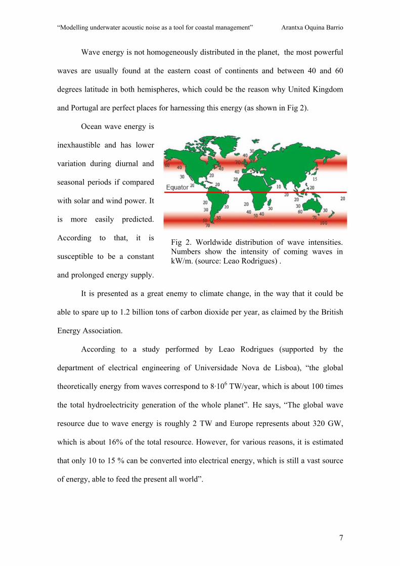
Wave energy is not homogeneously distributed in the planet, the most powerful
waves are usually found at the eastern coast of continents and between 40 and 60
degrees latitude in both hemispheres, which could be the reason why United Kingdom
and Portugal are perfect places for harnessing this energy (as shown in Fig 2).
Ocean wave energy is
inexhaustible and has lower
variation during diurnal and
seasonal periods if compared
with solar and wind power. It
is more easily predicted.
According to that, it is
susceptible to be a constant
and prolonged energy supply.
It is presented as a great enemy to climate change, in the way that it could be
able to spare up to 1.2 billion tons of carbon dioxide per year, as claimed by the British
Energy Association.
According to a study performed by Leao Rodrigues (supported by the
department of electrical engineering of Universidade Nova de Lisboa), “the global
theoretically energy from waves correspond to 8·106 TW/year, which is about 100 times
the total hydroelectricity generation of the whole planet”. He says, “The global wave
resource due to wave energy is roughly 2 TW and Europe represents about 320 GW,
which is about 16% of the total resource. However, for various reasons, it is estimated
that only 10 to 15 % can be converted into electrical energy, which is still a vast source
of energy, able to feed the present all world”.
Fig 2. Worldwide distribution of wave intensities. Numbers show the intensity of coming waves in kW/m. (source: Leao Rodrigues) .

“Modelling underwater acoustic noise as a tool for coastal management” Arantxa Oquina Barrio
8
However, despite solar and wind power having been widely extended and deeply
studied, and appearing as viable at present, marine energy has always stayed in their
shadow, due to its difficulty of harnessing. Nevertheless, there are many studies which
have been carried out in the last decades on marine energy sources and their feasibility,
becoming a promising electricity source. Numerous marine energy harnessing devices
have been widely presented either shoreline, nearshore and offshore, such as
Oscillating Water column, Limpet, Aquabuoy, Oyster, Pelamis Wave Energy
Converter, Wave dragon, to cite some of them (examples shown in figures 3, 4, 5).
Some of these devices appear finally just as theoretical ideas, but some others
overpass all the trials and experimenting phases and are already implemented into the
field. There have been many ideas for marine energy supply, but technical and practical
problems normally arose when these devices were studied in greater depth. One of the
main problems, for example, is the fact that those new energy harnessing offshore
devices underestimate the power of the sea, and then present a lack of capacity to resist
its force.
The current study focuses on OREDs, therefore offering the availability of
a higher energy resource, as they are situated offshore. Waves on offshore zone, are
supposed to be more energetic than those reaching the coastline. That is the reason why
Fig 3,4,5. Figures showing the Limpet, Wave dragon, and Oyster devices respectively. Source: Limpet uses power of marine waves on-shore, wave dragon is an off-shore device, and Oyster system is placed on the sea bottom. Sources: www.wavegen.co.uk , www.wavedragon.net, www.aquamarinepower.com.

“Modelling underwater acoustic noise as a tool for coastal management” Arantxa Oquina Barrio
9
any device located offshore will be susceptible to harness more energy from waves than
those located along the coastline.
Though they imply more difficult access, need of sophisticated technologies, the
added difficulty of energy transmission to land, and although nowadays there are less
environmental constraints, prototypes have still to be tested and research on them is
being carried out.
Although firms and investors want to improve these projects, and higher
development and studies are being carried out, installing the devices is also expensive,
and this energy can not normally compete with the great oil companies’ economic
infrastructures. But as soon as extraction of marine energy becomes economically
profitable, there is no doubt that it would become a great contribution for the worldwide
energy supply, as the length of coasts susceptible of accommodating this kind of
devices is very high. So there are some advantages of wave energy, as operation and
maintenance is not so expensive, no waste is produced, the liquids used do not contain
any pollutant and no toxic paints or treatments are used. But there are also main
disadvantages: this energy depends totally on wave intensity and thus on installation
location, and this can affect the environment by generating underwater acoustic hum,
which can cause many harmful effects on environment. It is paramount to remember
that the importance of wave power does not rely on the supply itself, but on an
alternative to reach the energetic requirements at local and regional scale, combined
with other energy sources.
3.2. General aspects of underwater acoustics.
Sound is a form of mechanical energy, a vibration that travels as a wave by causing
pressure changes in a fluid. Sound propagation, as said in the previous sections, is not

“Modelling underwater acoustic noise as a tool for coastal management” Arantxa Oquina Barrio
10
the same as in the air when the propagation channel is the ocean. The main importance
of sound within the ocean resides in the fact that the ocean is transparent to acoustic
waves, while practically opaque to electromagnetic radiations. It seems to be the only
radiation that can be propagated through long distances within the sea, especially at
lower frequencies.
The main variable affecting sound propagation in the ocean is sound speed.
Sound celerity is normally related to density and compressibility. Sound celerity in the
ocean is presented as an oceanographic
variable, which is a function of three
main parameters: depth, salinity and
temperature. Sound speed increases both
with temperature and pressure (Fig 6).
This dependence can be seen in the
empirical simplified expression for the
determination of sound celerity (Jensen
& Kuperman, 1994):
c = 1449.2 + 4.6 T – 0.055 T2 + 0.0029 T3 + (1.34 – 0.01 T) (S-35) + 0.016 z; (Eq. 1)
where temperature must be given in
Celsius, salinity in parts per thousand
and depth in meters.
Then it also varies with season,
diurnal changes, geographical location,
and time, as these parameters affect the
oceanographic conditions of the water
column (affecting indirectly the three
Fig 7. Generic sound speed profile within the ocean water column. (Source: Jensen & Kuperman, 1994)
Fig 6. General variation of sound speed with salinity (green), pressure (red) and temperature (blue) in fig (a) and sound speed resultant in fig (b).
“Modelling underwater acoustic noise as a tool for coastal management” Arantxa Oquina Barrio
11
parameters mentioned above: T, S, z).
Special attention has to be paid to the sound speed profile in the ocean, noting
the high decrease on its values in the existence of thermocline, however increasing with
depth since the deep sound channel axis. A typical value of 1500 m/s is normally given,
even though sound speed varies with oceanographic parameters, and is not
homogeneously presented within the ocean. A generic sound speed profile is shown in
Fig 7. There is a decrease on the sound profile from surface to depth due to decreasing
temperature (higher in surface because of sun heating, decreasing because of cooling
with depth). When temperature becomes mainly constant, pressure is the main factor
affecting sound speed, and as it increases linearly with depth, sound velocity also
increases linearly. Salinity does not have a great impact in open ocean, where no
significant changes occur, while it can be important in shallow waters, estuaries, or
closed areas, in other words, in those parts of the ocean where an important halocline is
occurring.
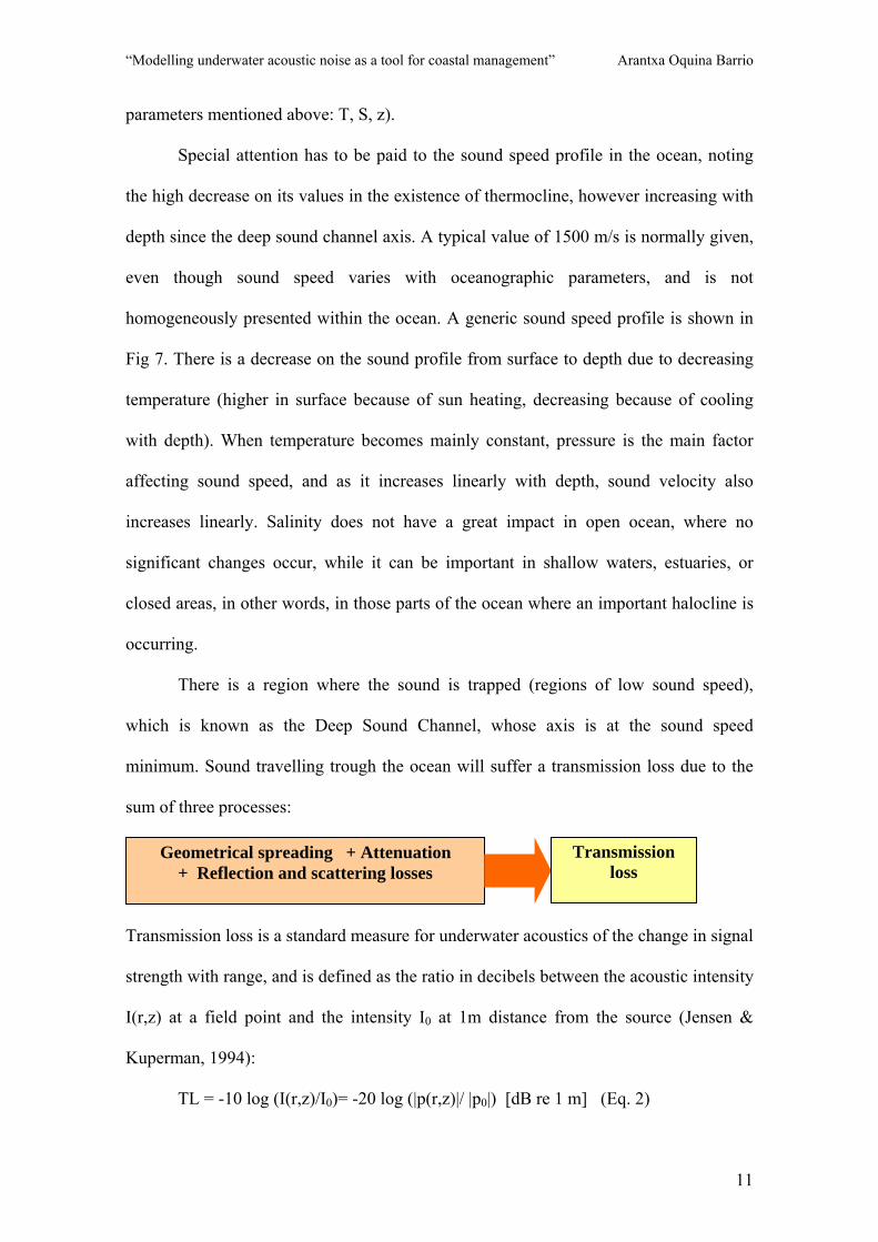
There is a region where the sound is trapped (regions of low sound speed),
which is known as the Deep Sound Channel, whose axis is at the sound speed
minimum. Sound travelling trough the ocean will suffer a transmission loss due to the
sum of three processes:
Transmission loss is a standard measure for underwater acoustics of the change in signal
strength with range, and is defined as the ratio in decibels between the acoustic intensity
I(r,z) at a field point and the intensity I0 at 1m distance from the source (Jensen &
Kuperman, 1994):
TL = -10 log (I(r,z)/I0)= -20 log (|p(r,z)|/ |p0|) [dB re 1 m] (Eq. 2)
Geometrical spreading + Attenuation + Reflection and scattering losses
Transmission loss
“Modelling underwater acoustic noise as a tool for coastal management” Arantxa Oquina Barrio
12
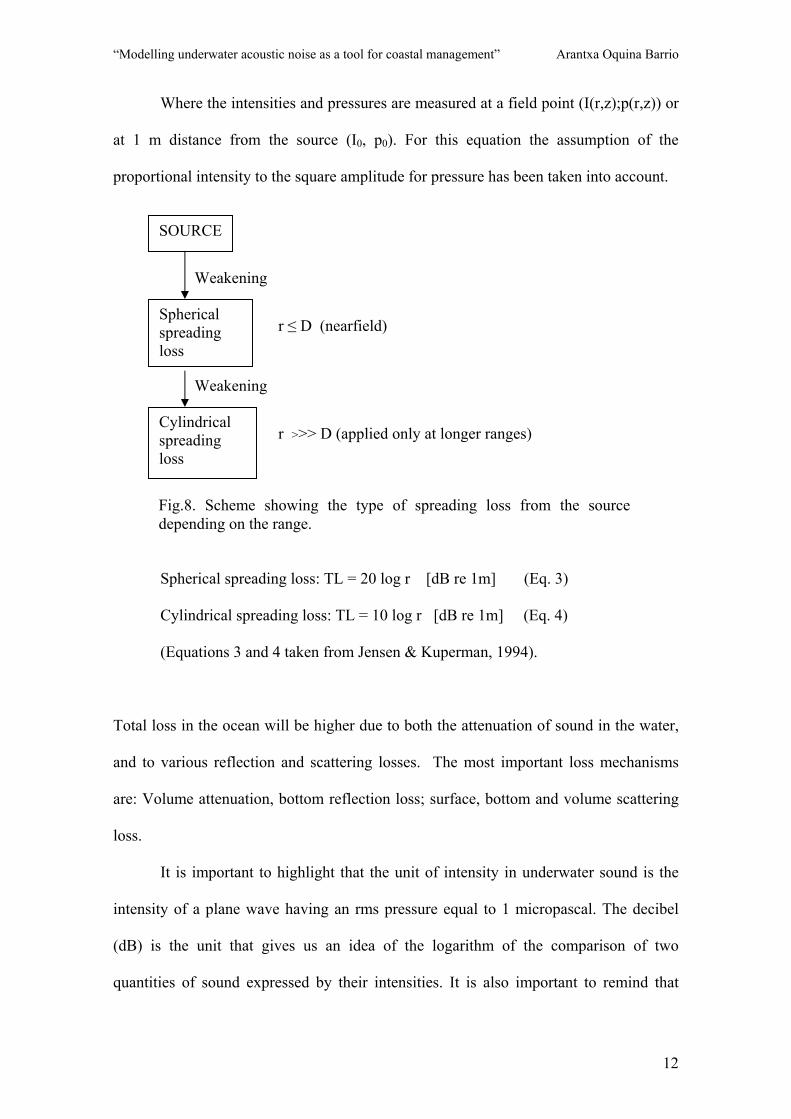
Where the intensities and pressures are measured at a field point (I(r,z);p(r,z)) or
at 1 m distance from the source (I0, p0). For this equation the assumption of the
proportional intensity to the square amplitude for pressure has been taken into account.
Spherical spreading loss: TL = 20 log r [dB re 1m] (Eq. 3)
Cylindrical spreading loss: TL = 10 log r [dB re 1m] (Eq. 4)
(Equations 3 and 4 taken from Jensen & Kuperman, 1994).
Total loss in the ocean will be higher due to both the attenuation of sound in the water,
and to various reflection and scattering losses. The most important loss mechanisms
are: Volume attenuation, bottom reflection loss; surface, bottom and volume scattering
loss.
It is important to highlight that the unit of intensity in underwater sound is the
intensity of a plane wave having an rms pressure equal to 1 micropascal. The decibel
(dB) is the unit that gives us an idea of the logarithm of the comparison of two
quantities of sound expressed by their intensities. It is also important to remind that
Weakening
Weakening
SOURCE
Spherical spreading loss
Cylindrical spreading loss
r ≤ D (nearfield)
r >>> D (applied only at longer ranges)
Fig.8. Scheme showing the type of spreading loss from the source depending on the range.
“Modelling underwater acoustic noise as a tool for coastal management” Arantxa Oquina Barrio
13
standard reference pressures for water and air are not the same, and thus noise levels
from both mediums cannot be compared directly. And as decibels are logarithmic
values, it must be said that two noise levels cannot be simply summed.
There remains a big importance in treating the ocean bottom accurately in the
numerical models. Numerical models depend on factors such as source-receiver
separation source frequency, and ocean depth. Bottom interaction is in general
unimportant for large ranges, high frequencies, and deep water, but crucial for short-
range, low frequency or shallow-water
propagation.
Sound will be naturally
produced by other noise sources, and
there will also be an introduction of
noise into the environment derived from
human activities.
Sounds which will naturally be
produced within the ocean will create
the existence of a constant ambient
noise within it. As natural sound sources
into the ocean we find: earthquakes,
volcanic tremors, lightning to the sea surface, wind and waves, and the voices, calls,
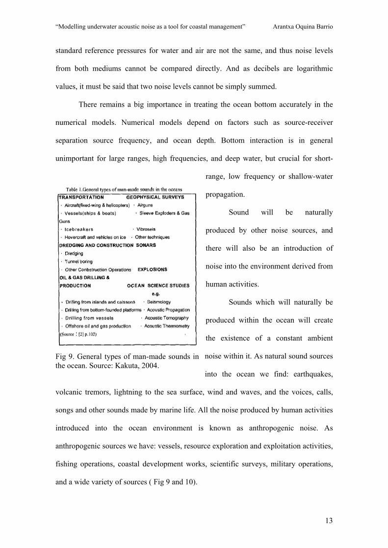
songs and other sounds made by marine life. All the noise produced by human activities
introduced into the ocean environment is known as anthropogenic noise. As
anthropogenic sources we have: vessels, resource exploration and exploitation activities,
fishing operations, coastal development works, scientific surveys, military operations,
and a wide variety of sources ( Fig 9 and 10).
Fig 9. General types of man-made sounds inthe ocean. Source: Kakuta, 2004.

“Modelling underwater acoustic noise as a tool for coastal management” Arantxa Oquina Barrio
14
Shallow water
For the acoustical propagation of sound in shallow waters, the ocean appears as
a channel, where the upper part is limited by the sea surface and the lower part by the
sea-floor. Both limits present a roughness related with scattering and attenuation of
sound. The current situation is that wavelength is comparable to water depth, and
depending on the relation between them sound will be propagated in several different
manners. This is related with the pathway followed by the sound transmission as it
encounters both limits being either refracted, reflected or absorbed. Thus, surface,
volume and bottom properties are all important. They vary spatially and generally are
not well enough known for an accurate prediction. Many reflection and absorption
processes are related with those boundaries in the case of sound propagation through
shallow water.
Fig.10. Natural and human-made source noise comparisons. Source: Kakuta, 2004
“Modelling underwater acoustic noise as a tool for coastal management” Arantxa Oquina Barrio
15
Cylindrical spreading is improved at shorter ranges, and the increased boundary
interaction degrades transmission at longer ranges (Jensen & Kuperman, 1994).
Sound speed profile varies with currents, heating and cooling, and tends to be
irregular and unpredictable. Sound speed for shallow water is known to be range
dependent, which means that it is not horizontally stratified, and it can not be
considered in range and depth separately, which complicates the calculations.
Many bottom interactions occur in shallow water, which appears to be very
important in the determination of sound propagation in this case. Bottom presents
layering, with different densities and sound speeds, the porosity of materials affecting
the density and thus propagation within the water column. Absorption from bottom
increases with increasing frequency. Geo acoustic parameters are normally not
particularly known for their inclusion in the sound propagation studies. All the
characteristics mentioned above, converts the sound propagation in shallow waters, in
a complex task for study.
3.3. Modelling processes
Measuring and researching acoustic signals in the ocean, normally requires extensive
equipment. Measuring also present a high difficulty according to the properties (range
dependence, complicated dependence on acoustic frequency) and inaccessibility of the
means. That is the reason why modelling acoustic signals and being able to make
predictions trough the utilization of modelling processes is so important.
Modelling the underwater acoustic propagation is made basically by solving
either the wave equation or the Helmholtz equation (reduced wave equation). This
procedure implies a high complexity due to the various acoustical environmental
conditions described in the previous section. Some of those variables could be sound
“Modelling underwater acoustic noise as a tool for coastal management” Arantxa Oquina Barrio
16
speed profile, depth and range variations, bottom characteristics related with the
appearance of shear, presence of interface waves, and many others. Resolution of the
wave equation would imply the determination of the sound field (intensity and phase).
Thus, a variety of numerical techniques has been developed, even though none of them
is capable to include all possible environmental conditions, frequencies and
transmission ranges of interest. (Buckingham, 1992)
Most of the propagation models made until the present have been considering
sound propagation in 2D. This means a limitation in shallow waters, where obliquely
incident rays are reflected from the bottom into a different vertical plane. That is called
“horizontal refraction”, and requires a 3D modelling, where the sound field is given in
depth and range, but also in azimuth. The so called 2 ½ D or Nx2D models are
intermediate solutions which give the field in range and depth, but applied over a large
number (N) of bearing angles. (Buckingham, 1992)
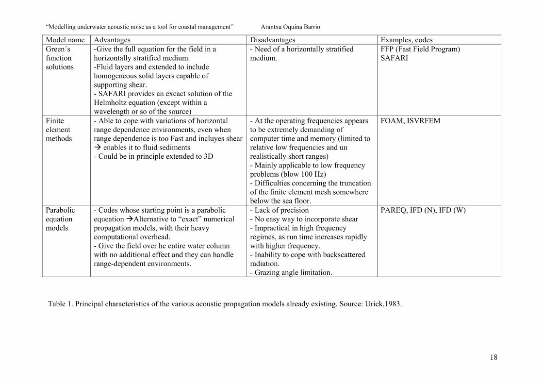
Five principal deterministic models can be mentioned for describing sound
propagation within the sea (deterministic because they neglect the effect of fluctuations
in the sound speed profile by small scale turbulences, internal waves, etc):
- Ray tracing.
- Normal mode techniques.
- Green’s function solutions.
- Finite element methods.
- Parabolic equation models.
Their principal characteristics are described in Table 1, where advantages and
disadvantages, and some examples of each model are shown.

“Modelling underwater acoustic noise as a tool for coastal management” Arantxa Oquina Barrio
17
Model name Advantages Disadvantages Examples, codes Ray models - Advisable for deep water problems, where
only a few rays are significant. - Fast to compute. - Pictorial representation through ray diagrams of the rays in the channel. - Easy to accommodate directionality of source and receiver. -Rays can be traced through range-dependent sound speed profiles and over complicated bathymetry.
- Difficulties in keeping track of phase at bottom reflections. - So many rays have to be traced. - Computations must be performed at all ranges out of the receiver. - Wave effects (diffraction and caustics) cannot be handled satisfactorily limitation for bottom interactions and low frequency propagation. - May generate false caustics and produce shadow zones. - Shear waves in an elastic bottom are beyond the capabilities of ray tracing models.
GRASS (Germinating Ray Acoustics simulation System), PLRAY (ray Propagation Loss), FACT (Fast Asymptotic Coherent Transmission), RAYMODE.
Normal mode techniques
- Mode functions do not have to be calculated at all intermediate ranges between source and receiver. (mode functions in deep, stable part of the water column are calculated and stored in advance, saving computation time). - It can be used either for range-independent environments (coupled model), or range-dependent environments (uncoupled models) if range dependence is low. - Suitable for low frequency or shallow water applications where the number of models is small.
- Most of them do not include branch line contribution, not handling shear in the bottom.
FFP (Fast field program) sometimes required Coupled model: COUPLE Uncoupled models: SNAP, SUPERSNAP, KRAKEN
“Modelling underwater acoustic noise as a tool for coastal management” Arantxa Oquina Barrio
18
Model name Advantages Disadvantages Examples, codes Green´s function solutions
-Give the full equation for the field in a horizontally stratified medium. -Fluid layers and extended to include homogeneous solid layers capable of supporting shear. - SAFARI provides an excact solution of the Helmholtz equation (except within a wavelength or so of the source)
- Need of a horizontally stratified medium.
FFP (Fast Field Program) SAFARI
Finite element methods
- Able to cope with variations of horizontal range dependence environments, even when range dependence is too Fast and incluyes shear
enables it to fluid sediments - Could be in principle extended to 3D
- At the operating frequencies appears to be extremely demanding of computer time and memory (limited to relative low frequencies and un realistically short ranges) - Mainly applicable to low frequency problems (blow 100 Hz) - Difficulties concerning the truncation of the finite element mesh somewhere below the sea floor.
FOAM, ISVRFEM
Parabolic equation models
- Codes whose starting point is a parabolic equeation Alternative to “exact” numerical propagation models, with their heavy computational overhead. - Give the field over he entire water column with no additional effect and they can handle range-dependent environments.
- Lack of precision - No easy way to incorporate shear - Impractical in high frequency regimes, as run time increases rapidly with higher frequency. - Inability to cope with backscattered radiation. - Grazing angle limitation.
PAREQ, IFD (N), IFD (W)
Table 1. Principal characteristics of the various acoustic propagation models already existing. Source: Urick,1983.
“Modelling underwater acoustic noise as a tool for coastal management” Arantxa Oquina Barrio
19
3.4. Main effects of underwater acoustic noise over the environment.
As said in the previous section, marine environment is constantly exposed to an ambient
noise. Marine organisms are used to this ambient noise caused by natural sources. The
problem appears with the introduction into the environment of an additional man-made
noise.
Any organism has the necessity of communicating with its environment, and in
terrestrial animals, this communication can be done through the five senses. In the
marine environment, light is attenuated in the first meters of depth, being practically
inexistent reaching certain depths in the ocean. As a result, vision is a limited sense in
the ocean. Nevertheless, sound, as seen in the previous section, is in comparison quite
easily propagated within the medium, which in fact, leads it to be presented as the basic
communication tool among some marine organisms and their environment. Therefore,
there are numerous marine organisms, such as marine mammals which use sound as
their principal sense for the so called “echolocation”, inter and intraspecies
communication, and detection of preys and predators.
Numerous studies have been carried out to determine the effect that
anthropogenic underwater sound is capable to cause over marine mammals. By the
middle of the 20th century seismic prospecting, marine transport by vessels, sonar,
explosions and industrial activities are presented as the main anthropogenic underwater
acoustic noise sources in the ocean, and are getting more and more frequently
encountered in the medium. All those sources generate a noisy ocean with a high short-
term acoustic pollution, which requires urgent monitoring. This noise appears to be
interfering in communication, orientation and feeding of marine mammals. Conflict
with evolutionarily-adapted sound-sensing marine mammals seems inevitable (Lopez et
al, 2003). Also fish use sound for communicating, principally in the mating process,
“Modelling underwater acoustic noise as a tool for coastal management” Arantxa Oquina Barrio
20
though there is much less research on the effects that introduction of noise can cause in
this case.
A general description of the way marine mammals use sound will be given in
this section. First of all, adaptations in marine mammals are not reduced to the use of
sound as a hearing sense, but appear also in the morphology of their auditive system. In
this sense, they present differences in their organs compared to terrestrial mammals.
Their inner ear is similar, while their medium ear is largely modified and their external
ear is almost inexistent.
Most of marine mammals studied use echolocation, which means they use sound
for exploring their surrounding and for communicating. There is a wide range of
frequencies in which marine mammals can produce and hear sounds, depending
basically on the physical properties of the environment.
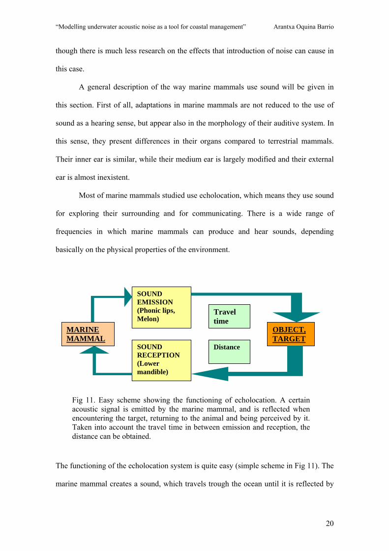
The functioning of the echolocation system is quite easy (simple scheme in Fig 11). The
marine mammal creates a sound, which travels trough the ocean until it is reflected by
MARINE MAMMAL
SOUND EMISSION (Phonic lips, Melon)
SOUND RECEPTION (Lower mandible)
OBJECT, TARGET
Travel time
Distance
Fig 11. Easy scheme showing the functioning of echolocation. A certain acoustic signal is emitted by the marine mammal, and is reflected when encountering the target, returning to the animal and being perceived by it. Taken into account the travel time in between emission and reception, the distance can be obtained.
“Modelling underwater acoustic noise as a tool for coastal management” Arantxa Oquina Barrio
21
an object and returns to the cetacean, which receives the signal. Depending on the time
the sound takes to go and return, and depending on the properties of the sea the distance
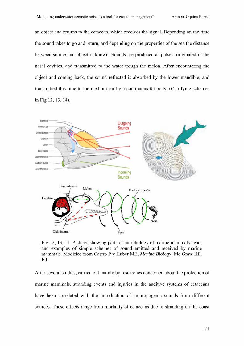
between source and object is known. Sounds are produced as pulses, originated in the
nasal cavities, and transmitted to the water trough the melon. After encountering the
object and coming back, the sound reflected is absorbed by the lower mandible, and
transmitted this time to the medium ear by a continuous fat body. (Clarifying schemes
in Fig 12, 13, 14).
After several studies, carried out mainly by researches concerned about the protection of
marine mammals, stranding events and injuries in the auditive systems of cetaceans
have been correlated with the introduction of anthropogenic sounds from different
sources. These effects range from mortality of cetaceans due to stranding on the coast
Fig 12, 13, 14. Pictures showing parts of morphology of marine mammals head, and examples of simple schemes of sound emitted and received by marine mammals. Modified from Castro P y Huber ME, Marine Biology, Mc Graw Hill Ed.
“Modelling underwater acoustic noise as a tool for coastal management” Arantxa Oquina Barrio
22
caused by loss of direction, to injuries in the auditive system, which can range also from
minor and temporally, to severe and permanent (Lopez et al, 2003). The threshold from
effects proposed by those scientists, are based on these two types of injuries.
Nevertheless, current scientific knowledge regarding the effects on marine mammals
and their habitat is not enough to understand the relation between frequencies,
intensities and duration of exposure and the cause of adverse consequences. All this
implies that it is necessary to perform more exhaustive and deep research on the effects
of underwater acoustic noise on cetaceans. This research will be used to develop and
implement either mitigation methods, limits for activities causing noise in certain zones
where cetaceans concentrate, and objective parameters for advising conservation of
marine biodiversity design, needed for establishing international and European norms
on acoustic marine pollution (Greenpeace and Spanish Cetaceans Society, 2003)
The principal impacts caused by the introduction of underwater acoustic noise
into the environment can be divided mainly into three categories: 1) masking,
2) disturbance, 3) effects on sensitivity of hearing.
So, the main studies carried out on cetaceans were “focused primarily on
understanding criteria and thresholds for physiological and behavioural effects, location
and abundance of marine mammals, and sound source characteristics and propagation
paths” (Hastings, 2008). Some standard reference levels were set after those studies, in
relation to sound intensity and effects on marine animals. Those effects could be tissue
damage, changes in hearing sensitivity and/or changes in behavioural aspects, which are
related with age, sex, activity engaged in at the time of exposure. Subsequently to these
bioacoustic experiments, some threshold values are fixed for the different species,
depending on the duration of effects:

“Modelling underwater acoustic noise as a tool for coastal management” Arantxa Oquina Barrio
23
- Temporary threshold shift (TTS) if hearing threshold returns to the pre-
exposure level
- Permanent threshold shift (PTS) if threshold does not return to pre-
exposure levels.
Both TTS and PTS, are correlated with the so called sound exposure level (SEL),
measured for several different types of sound sources. (Hastings, 2008).
3.5. Acoustic noise policies and implications on management.
According to the 1982 United Nations convention on the Law of the Sea (UNCLOS),
“States have the obligation to protect and preserve the marine environment”, as cited in
Article 192. This is the first time that this obligation is explicitly required in a global
treaty.
By this convention marine pollution is defined as: “the introduction by man,
directly or indirectly, of substances or energy into the marine environment, including
estuaries, which results or is likely to result in such deleterious effects as harm to living
resources and marine life, hazards to human health, hindrance to marine activities,
including fishing and other legitimate uses of the sea, impairment of quality for use of
sea water and reduction of amenities”. Noise is a form of energy, such as heat and
radiation, which is introduced into the sea by different ways. Its deleterious effects on
marine animals have been studied in several occasions, resulting in the ability of loud
sounds to injure or kill marine mammals. For those reasons, noise can be considered
a pollutant according to the convention. Heat and radiation were previously studied and
regulated in other occasions, but noise has not been included as a pollutant in any
convention till this point.
“Modelling underwater acoustic noise as a tool for coastal management” Arantxa Oquina Barrio
24
Noise must be treated as a transboundary pollutant, and the UNCLOS is also
focusing its effort on this part, by Article 194: “States shall take all measures necessary
to ensure that activities under their jurisdiction or control are so conducted as not to
cause damage by pollution to other states and their environment, and that pollution
arising from incidents or activities under their jurisdiction or control does not spread
beyond the areas where they exercise sovereign rights in accordance to this
Convention”. And referring to the cooperation between nations or regions cited in
Article 197, “States shall cooperate on a global basis and, as appropriate, on a regional
basis, directly or through competent international organizations, in formulating and
elaborating international rules, standards and recommended practices and procedures
consistent with this Convention, for the protection and preservation of the marine
environment, taking into account characteristic regional features”.
Article 204 on the UNCLOS refers to the need for monitoring and research.
Article 206 refers to the necessity of previous environmental plans before the activities
take place.
Although UNCLOS gives the perfect framework for pollution prevention and is
susceptible to include new forms of pollutants such as noise (also because a part
referred to marine mammals protection is included), it is still not specific about the
requirements for States to deal with these pollutants. It does not treat the problem of
underwater acoustic noise itself.
About the existing regulatory framework on underwater acoustic noise some
facts are found which turns it regulation difficult: its transboundary nature, and the lack
of knowledge regarding its effects. There are still no international agreements or
international organizations responsible for that.

“Modelling underwater acoustic noise as a tool for coastal management” Arantxa Oquina Barrio
25
Nevertheless, an overview of the regulatory framework on underwater acoustic noise
(McCarthy, 2004) will be done, through a brief view on the existing cooperative
agreements and international bodies with an important role involved:
- United Nations Environmental Programme (UNEP), does not refer to
underwater acoustic noise as a pollutant, but refers to it in its publication
“Marine Mammals: Global Plan of Action”.
- The international Maritime Organization (IMO), does not include
underwater acoustic noise as a pollutant on its main Protocol of 1978
(MARPOL); but includes the creation of Particularly Sensitive Sea Areas
(PSSAs), which include even noise among the possible pollutants within
the marine area.
- The International Whaling Commission (IWC), which addresses the
disturbance noise effects of vessels on marine mammals.
- The International Seabed Authority (ISBA) shows no legal standards with
reference to noise and acoustic disturbances.
- The European Union, protects marine mammals by the Council Directive
92/43/ECC on the conservation of Natural Habitats and of Wild Fauna and
Flora, but makes no explicit reference to noise. The European Union
perceives the necessity of the development of international agreements for
the regulation of noise in the ocean.
The latest news related to acoustic noise pollution from the European
Commission Research (European Commission Research News, 2004) is presenting
actions for the creation of a European normative related to the air noise pollution, but no
reference to acoustic noise pollution is done. A European Directive related with sound
(European Environmental Noise Directive, DIRECTIVE 2002/49/EC) was found to be
“Modelling underwater acoustic noise as a tool for coastal management” Arantxa Oquina Barrio
26
related only with air noise pollution, with no reference to underwater acoustic noise
pollution was made but only references to human impacts.
More information about research over acoustic noise and its impact on marine
mammals has currently been done by USA, most of it related with specific sound
systems, such as military sonar, Surtass LFA, and others. Committees on Sound and
Marine Mammals have been established and produce reports on the state of knowledge
and recommendations for changes in the regulatory process as well as facilitating tools
and supporting the evaluation of effects of underwater noise. (Hastings, 2008). It is in
the USA where most legislative development for underwater acoustic noise has been
done; some important protection figures related with marine mammals and sound
appears with the Marine Mammals Protection Act (MMPA), the Endangered Species
Act (ESA). They have both joined the NOAA for running some programmes of research
and protection which have been derived in some legislation forums and characters.
There is a report by the NOAA symposium of 2004, “Shipping Noise and Marine
Mammals”, which makes references to underwater acoustic noise, but only the one
produced by maritime traffic.
Returning to the European case, the European Cetacean Society presents
a statement on marine mammals and sound on its web site as follows:
1) Research on the effects of man-made noise on marine mammals is urgently
needed, and must be conducted to the highest standards of science and public
credibility, avoiding conflicts of interest.
2) Non-invasive mitigation measures must be developed and implemented as
soon as possible
“Modelling underwater acoustic noise as a tool for coastal management” Arantxa Oquina Barrio
27
3) The use of underwater powerful noise sources should be limited until their
short- and long-term effects on marine mammals are better understood, and they should
not be used in areas of importance for cetaceans.
4) Legislative instruments that help to implement both national and European
policies on marine noise pollution must be developed.
Underwater acoustic noise resulting from the installation of off-shore devices
appears as a significant pollution source in the environment, but still not proper
attention has been paid to the anticipated impact that man-made noise can produce.
(Kakuta, 2004)
There has been a workshop in San Sebastian (SPAIN) in 2007 by the European
cetacean society and the UNEP/ASCOBANS, where relation between wind farms and
cetaceans has been deeply discussed, but still, not even the relation with other ORED
(Off-shore Renewable Devices) has been studied.
“In the absence of data, scientists and government regulators have always been
precautionary in recommending noise exposure criteria for marine animals” (Hastings,
2008)
As an example of some threshold criteria “NOAA Fisheries set a sound pressure
limit of 180 db re 1μPa that could not be exceeded for mysticetes and sperm whales,
and 190 db re 1μPa for most odontocetes and pinnipeds” (Hastings, 2008)
“Finally, in order to begin to understand “biologically significant” effects on
behaviour as defined within the framework outlined in the latest NRC report (NRC,
2005), multi-disciplinary basic research is needed to understand the primary and
synergistic effects of sound on marine ecosystems, including crustaceans, corals,
sponges, sea grasses, and all other living things in the sea. Designing experiments to
learn about potential changes in the marine ecosystem, including animal habitats, over

“Modelling underwater acoustic noise as a tool for coastal management” Arantxa Oquina Barrio
28
long periods of time is a very difficult task. But changes in the behavior and habitats of
marine animals over the long term could significantly affect their populations as well as
the overall health and stability of the marine environment” (Hastings, 2008)
Even though there is a lack of concrete and reliable legislation over acoustical
impacts on marine mammals, there are several protection figures related to them. Those
legislative figures on marine mammals could also be used in management plans for
industrial projects.
“ One way to assess the impact of ocean noise is to consider whether it causes
changes in animal behaviour that are “biologically significant”, that is, those that affect
an animal´s ability to grow, survive, and reproduce.” (NRC, 2005)
In this direction, main protective figures over cetaceans will be named (Atlas of
Cetacean, 2003):
- Bern Convention, implemented in 1982: common dolphin, bottlenose
dolphin, harbour porpoise, blue whale, humpback whale, northern right
whale and bowhead whale are under strict protection by Appendix II.
- Bonn Convention, implemented in 1983: blue whale, humpback whale,
bowhead whale, and northern right whale, are under strict protection in
Appendix I, on the Convention of Migratory Species.
- EU Habitats and Species Directive (1992): Annex 2 includes harbour
porpoise and bottlenose dolphin as `animal and plant species whose
conservation require designation of Special Areas of Conservation´
- OSPAR, Oslo-Paris Convention (1992): bowhead whale, northern right
whale, blue whale and harbour porpoise are included in its first list of
threatened and declining species.

“Modelling underwater acoustic noise as a tool for coastal management” Arantxa Oquina Barrio
29
- UNCLOS, United Nations Convention on the Law Of the Sea (1995): where
“including the preservation and protection of the marine environment and the
conservation of marine living resources both within and beyond national
jurisdiction” appears as fundamental obligation.
After that, referring to the case of Portugal, the Ministério da qualidade de vida, on its
“Decreto lei nº 263/81”, makes a special regulation for the protection of marine
mammals within the coastal and Economic Exclusive Zone, and publishes a list of
cetaceans which are under special protection by this law.
3.6. The DPSIR framework for management.
The DPSIR framework has been adopted by the European Environment Agency (EEA),
and is a causal framework used in Integrated Coastal Zone Management (ICZM) for the
Environmental Impact Assessment (EIA). It is used to describe the interactions between
ecological, economical and social aspects. It enables to create basic schemes for
presenting all the information needed for policy makers and the decision-making
process. DPSIR framework is useful to identify the dynamics between origin and
consequence of environmental problems, by following the causal chain shown in figure
15. The main goal of this scheme is to give a structure for data and information on
diverse environmental problems. This structure and the environmental indicators used
on it will be useful for communicating environmental information to the policy makers
and the public.

“Modelling underwater acoustic noise as a tool for coastal management” Arantxa Oquina Barrio
30
The basic components of the DPSIR framework (Martin Le Tissier) are mainly:
- DRIVING FORCES: they are the needs. It can be primary driving forces as
shelter, food and water; and secondary driving forces such as mobility,
entertainment and culture.
- PRESSURES: Human activities from driving forces, creates pressures in the
environment. These pressures can be divided into excessive use of
Fig 15. Basic elements susceptible of being found in a general DPSIR scheme. (Source: Global international Water assessment, 2001. http://maps.grida.no/go/graphic/the_dpsir_framework )
“Modelling underwater acoustic noise as a tool for coastal management” Arantxa Oquina Barrio
31
environmental resources, changes in land use, and emissions (chemicals,
waste, radiation, noise) to air water and soil.
- STATE OF THE ENVIRONMENT: Is the reaction of environment to the
pressures.
- IMPACTS: They can be on population, economy and ecosystems. Changes
in state may cause impacts derived from pressures.
- RESPONSES: they can be referred to as the responses by society, or policy
makers to an undesired impact. Those responses can affect some or all the
parts of the causal chain.
The process of determining the causal chain is complex and sometimes needs to be done
by determining subgroups on the different parts of the scheme as well as the interaction
between them. It is sometimes necessary to focus on some of these relationships for
a proper understanding of the entire scheme.
“Modelling underwater acoustic noise as a tool for coastal management” Arantxa Oquina Barrio
32
4. STUDY PROCEDURE
Some specific objectives will be set for the completion of the main objective as shown
in the table below:
SPECIFIC OBJECTIVES AT
STUDY CASE
METHODOLOGY
I. CASE STUDY
CHARACTERIZATION.
- Location and environmental characteristics
determination.
- Description of the offshore device.
- Determination of marine mammal
populations within the zone, the acoustic
frequency bands they use, and acoustic
thresholds set for noise effects.
- Determination of DPSIR scheme to follow
for management study.
II. MODELLING UNDERWATER
NOISE LEVEL. OBTAINING
SPATIAL DISTRIBUTION MAPS
- Use of matlab software for underwater
acoustic noise level modelling, through the
normal mode model KRAKEN.
- Underwater acoustic noise level distribution
map obtention.
III. VALIDATION OF THE
MODEL.
- Comparison of sound levels with cetacean
acoustic effect thresholds/acoustic bands.
- Demonstration of viability of modelling as a
tool for coastal management.

“Modelling underwater acoustic noise as a tool for coastal management” Arantxa Oquina Barrio
33
I. CASE STUDY CHARACTERIZATION:
Four main goals were supposed to be covered within this objective. First of all, location
of ORED and environmental characteristic of the area should be done. Afterwards,
knowledge of the device under study itself will be needed for the whole problem
understanding. Determination of the aspects of marine mammals related to the zone
under study, will be the next step. And finally, determination of the DPSIR scheme to
follow for management study.
Within the first goal, description of the area where the device is located will be
done. Referring to the environmental characteristics of the zone, mainly values for
depth, salinity, temperature, and then sound celerity would be needed (using the sound
celerity formula, Eq. 1). But also the sound characteristics of the noise source (the
device itself in our case), would be needed for an appropriate and accurate modelling.
Acoustical research in the field normally requires at-sea platforms equipped with
sound projectors, receiving arrays and sensors for measuring the environment. In our
case study, sound is already made by the device, and what is needed are sound levels at
certain points for making a matrix related to sound level, distance to the source and
depth, so a number of hydrophones should be set in the area. In our case study, the main
acoustic scheme would be shown in fig 22, where hydrophones should be in the primary
phase of receiving, and for the modelling. Even though, the final receivers, which
should be taken into account should be the marine mammals susceptible of being
affected by the underwater acoustic noise emitted by the Pelamis device:

“Modelling underwater acoustic noise as a tool for coastal management” Arantxa Oquina Barrio
34
An introduction to our specific ORED will be made in the next step. It is
important to know everything about our device in order to be able to determine whether
some aspects of our case study are important or not. An explanation about what is the
device and how it works is necessary for understanding the reasons for this case study.
In third step, determination of cetacean distribution within the zone would be
needed. It would also be useful to determine the state of conservation of those marine
mammal species present within the study area. Cetacean populations could be affected
directly by the noise produced by the source itself, or by the noise propagation trough
the ocean. Information about the frequency bands in which the marine mammals emit
and receive sounds would be needed. Nevertheless, some references of thresholds and
reaction levels would be desirable in order to compare our results with any values
already set before starting. Information about species within the zone was obtained by
interviewing some Portuguese experts in marine mammals (Marina Sequeira and Jose
Vingada), and by seeking results in cetacean researches made in Portugal. About
80 species are described worldwide, 23 of them in Portugal, and seven of them within
our study area. Results from three different sources agreed in species distribution,
although published and real data is still not available, but is being studied under the
SAFESEA project (reliable published data will be available in some years).
Data related with acoustic noise effect thresholds and sound references for
cetaceans will be taken from various studies, where we can find references of sound
Sound source: Pelamis device
Acoustic channel: Ocean
Sound receiver 1: hydrophones
Sound receiver 2: marine mammals Fig 16. Basic acoustical scheme for study.

“Modelling underwater acoustic noise as a tool for coastal management” Arantxa Oquina Barrio
35
levels emitted and received for each species under study, and in some cases the
threshold levels set for them. (Annex 1).
The determination of the DPSIR framework scheme has to be accurately done in
order to present the overall information in the most complete way for the manager
comprehension.
II. ACOUSTIC UNDERWATER NOISE SPATIAL DISTRIBUTION MAP
OBTENTION:
This part of the project will consist basically in the creation of a virtual scenario trough
acoustic modelling, which will allow the user to predict the sound level at each point in
the marine environment within the affected area.
Different types of models for solving the wave equation were reviewed in the
underwater acoustics section, and a table showing their principal characteristics was
given. As we assume to be in a shallow off-shore environment, which would not be
horizontally stratified and would be range-dependent mean, we assume that the best
type of model to use would be a normal mode model. Normal mode models give
a numerical solution to the wave equation by the usage of branch integrals. They are
suitable for low frequencies and shallow environments where the number of modes is
reduced. They normally take into account layered environments (water column and
bottom layer, at least). KRAKEN normal mode model is constituted by an algorithm.
This algorithm includes the elastic properties of the ocean bottom which enables it to
model ocean environments that are range-dependent, range-independent or even 3D
(consisting in infinite 2D superposed to create a 3D scenario). KRAKEN appears to be
a multilayered model, where roughness and elastic characteristics of layers can be
included.

“Modelling underwater acoustic noise as a tool for coastal management” Arantxa Oquina Barrio
36
The program that will be used for the modelling part will be implemented in
Matlab. Through the use of this program, KRAKEN normal mode model is supposed to
be used for obtaining a simulated map, which would give the acoustic sound levels at
each point from the marine environment within the study area.
After the completion of data compiling, the model will be ready to run, and after
that, an acoustic underwater noise spatial distribution map would be obtained as a result.
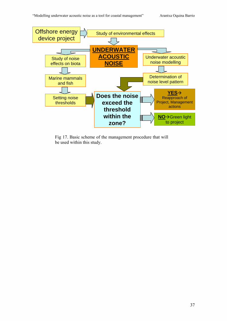
III. DEMONSTRATION OF VIABILITY OF MODELLING AS A TOOL FOR
COASTAL MANAGEMENT:
The question of the marine mammal’s threshold will be tried to answer in this part of
the project. Sound levels obtained by the simulation should not exceed the thresholds
set in previous studies. If it is possible to compare those values obtained by the map
with those within the studies done on cetaceans for setting thresholds, then a decision
upon the viability of the renewal energy device implementation could be done. In this
direction, if the sound levels obtained do not exceed the thresholds set before, the
environmental acoustic study over the zone will be positive, and the project will carry
on with its implementation and will remain active. If those sound levels exceed
significantly the thresholds, then further studies over device must be done or mitigation
measures taken into account. The following figure shows a simplified scheme of how
the viability demonstration could be done, and the steps to follow from the planning of
the device installation to the final decision-making (Fig 17).
“Modelling underwater acoustic noise as a tool for coastal management” Arantxa Oquina Barrio
37
YES Reapproach of
Project, Management actions
Offshore energy device project
Study of noise effects on biota
Underwater acoustic noise modelling
Marine mammals and fish
Setting noise thresholds
Study of environmental effects
UNDERWATER ACOUSTIC
NOISE
Determination of noise level pattern
Does the noise exceed the threshold within the
zone? NO Green light
to project
Fig 17. Basic scheme of the management procedure that will be used within this study.

“Modelling underwater acoustic noise as a tool for coastal management” Arantxa Oquina Barrio
38
5. CASE STUDY CHARACTERIZATION.
Our study will take place over the first commercial wave farm worldwide. It is located
in Aguçadoura, a town in Povoa de Varzim,
near the Portuguese city of Porto, in the north of
Portugal. The entire Portuguese coast is known
by the formation of waves coming from the
Atlantic Ocean. Those waves are mostly
permanent during the whole year, which makes
it a perfect suitable place for installing wave
energy devices (Fig 18).
There are two main reasons for the
establishment of this wave farm in Portugal.
First of all, Portugal is blessed with a good and
strong wave energy climate. Secondly, it has a proactive government that is developing
a favourable climate for wave energy demonstration projects and for further commercial
development of the wave energy market. “This project benefits from a special feed in
tariff established by the Portuguese Government to support the first wave energy
installations. The tariff of 25 cent €/kWh is higher than the one provided to wind energy
but lower than the one provided to solar energy. All of them are relatively mature
technologies which have enjoyed significant cost reductions over time through volume
production. The initial phase is also supported by the Demtec programme with
a 1.25 million € grant from the Agencia de Inovaçao (www.adi.pt).
For the environmental characterization of Povoa the Varzim, some data will be
required. First of all, temperatures within the water column through the year will be
needed. Fig 19 shows data referring to temperature profiles corresponding to
Fig 18. Map showing Povoa de Varzim, north of Portugal. Source: Google Earth

“Modelling underwater acoustic noise as a tool for coastal management” Arantxa Oquina Barrio
39
April 2004, July 2007 and October 2000. There is no presence of a significant
thermocline. April temperature profile appears to be so smooth varying only about 1º C
within the first 120 meters, while bigger differences are shown for July and October.
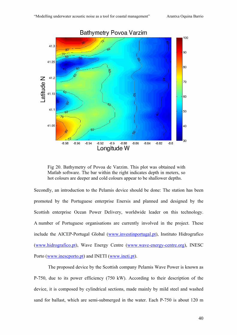
A plot for the bathymetry is shown in Fig 20 where the coast is left on the right side of
the figure, and the north is in the top of the figure. Depth has a general trend to grow
with distance to the coast. Nevertheless, two zones with shallower depth can be seen in
between 41.15º N and 41.1º N and 8.9º W and in between 41.20º N and 41.25º N and
8.98º W. Hot colours within the figure represent higher depths, while cold colours
represent shallower depths as given by the bar on the right of the figure.
Fig 19. Temperature profiles for three different seasons. This plot was obtained with Matlab software, and shows the temperature variation within the water column for three different seasons.
“Modelling underwater acoustic noise as a tool for coastal management” Arantxa Oquina Barrio
40
Secondly, an introduction to the Pelamis device should be done: The station has been
promoted by the Portuguese enterprise Enersis and planned and designed by the
Scottish enterprise Ocean Power Delivery, worldwide leader on this technology.
A number of Portuguese organisations are currently involved in the project. These
include the AICEP-Portugal Global (www.investinportugal.pt), Instituto Hidrografico
(www.hidrografico.pt), Wave Energy Centre (www.wave-energy-centre.org), INESC
Porto (www.inescporto.pt) and INETI (www.ineti.pt).
The proposed device by the Scottish company Pelamis Wave Power is known as
P-750, due to its power efficiency (750 kW). According to their description of the
device, it is composed by cylindrical sections, made mainly by mild steel and washed
sand for ballast, which are semi-submerged in the water. Each P-750 is about 120 m
Fig 20. Bathymetry of Povoa de Varzim. This plot was obtained with Matlab software. The bar within the right indicates depth in meters, so hot colours are deeper and cold colours appear to be shallower depths.

“Modelling underwater acoustic noise as a tool for coastal management” Arantxa Oquina Barrio
41
long and wit a diameter of 3.5 m, and has three conversion modules on it (each of them
with a length of 5 m and the same diameter). Each of the conversion modules has
a 250 kW electric generator, giving a total power of 750 kW for each Pelamis unit.
Functioning of the Pelamis device consists basically in the use of wave motion to get
movement of a hydraulic fluid (biodegradable in marine environment). It moves
similarly as a sea snake, from where it receives its name (the word pelamis in Greek
language means sea snake). As the
wave comes, Pelamis device adjusts
its movement to it as if it was a rope,
and every cylindrical section gets
moved up and down. This up-down
movement allows the hydraulic fluid
contained in the conversion modules
(in Fig 21) of Pelamis to activate
Fig 21. Basic movement made by Pelamis device. (Source: www.pelamiswave.com)
Fig 22. Scheme of a conversion module from Pelamis. (Source: www.pelamiswave.com/)

“Modelling underwater acoustic noise as a tool for coastal management” Arantxa Oquina Barrio
42
electrical generators driven by hydraulic motors, which leads to the production of
electricity (Fig 22).
As a result of the state of marine conditions waves will be variable, and so
“depending on the wave resource, machines will on average produce 25-40% of the full
rated output over the course of a year. Each machine can provide sufficient power to
meet the annual electricity demand of approximately 500 homes” (Pelamis web site)
Before the installation of the Pelamis device in Portugal, a series of trials in the
North Sea were previously performed in 2004 with a large scale commercial prototype
(Fig 23) which had the ability of supplying energy to
the UK grid. It took 18 months to check design with
one of the leading consultants in offshore structures
called Atkins, before building the machine, which had
initially a design life of 15 years. Critical test
objectives were run over the machine during an
extensive phase of testing. Success in this checking
made it possible to plan the installation in Portuguese waters for the first commercial
wave farm in 2006.
It was ten years before that Pelamis
Wave Power started developing Pelamis
technology (Fig 24). After completing the
development process, Pelamis Wave Power is
still running studies that will improve those
technological and economical aspects,
including the reduction in costs of installation,
maintenance and decommissioning.
Fig 23. Pelamis prototype device. (Source: www.pelamiswave.com/)
Fig 24. Pelamis device in off-shore location. (Source: www.pelamiswave.com/)
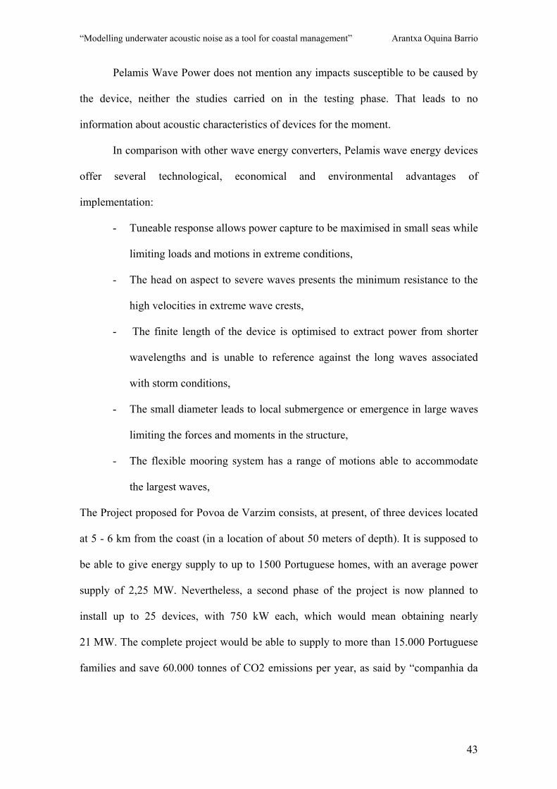
“Modelling underwater acoustic noise as a tool for coastal management” Arantxa Oquina Barrio
43
Pelamis Wave Power does not mention any impacts susceptible to be caused by
the device, neither the studies carried on in the testing phase. That leads to no
information about acoustic characteristics of devices for the moment.
In comparison with other wave energy converters, Pelamis wave energy devices
offer several technological, economical and environmental advantages of
implementation:
- Tuneable response allows power capture to be maximised in small seas while
limiting loads and motions in extreme conditions,
- The head on aspect to severe waves presents the minimum resistance to the
high velocities in extreme wave crests,
- The finite length of the device is optimised to extract power from shorter
wavelengths and is unable to reference against the long waves associated
with storm conditions,
- The small diameter leads to local submergence or emergence in large waves
limiting the forces and moments in the structure,
- The flexible mooring system has a range of motions able to accommodate
the largest waves,
The Project proposed for Povoa de Varzim consists, at present, of three devices located
at 5 - 6 km from the coast (in a location of about 50 meters of depth). It is supposed to
be able to give energy supply to up to 1500 Portuguese homes, with an average power
supply of 2,25 MW. Nevertheless, a second phase of the project is now planned to
install up to 25 devices, with 750 kW each, which would mean obtaining nearly
21 MW. The complete project would be able to supply to more than 15.000 Portuguese
families and save 60.000 tonnes of CO2 emissions per year, as said by “companhia da
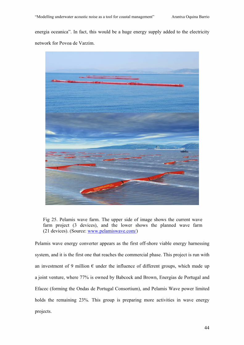
“Modelling underwater acoustic noise as a tool for coastal management” Arantxa Oquina Barrio
44
energia oceanica”. In fact, this would be a huge energy supply added to the electricity
network for Povoa de Varzim.
Pelamis wave energy converter appears as the first off-shore viable energy harnessing
system, and it is the first one that reaches the commercial phase. This project is run with
an investment of 9 million € under the influence of different groups, which made up
a joint venture, where 77% is owned by Babcock and Brown, Energias de Portugal and
Efacec (forming the Ondas de Portugal Consortium), and Pelamis Wave power limited
holds the remaining 23%. This group is preparing more activities in wave energy
projects.
Fig 25. Pelamis wave farm. The upper side of image shows the current wave farm project (3 devices), and the lower shows the planned wave farm (21 devices). (Source: www.pelamiswave.com/)

“Modelling underwater acoustic noise as a tool for coastal management” Arantxa Oquina Barrio
45
The installation of the pilot wave farm in Portugal, does not only allow the testing phase
in the real environment of the device, but also the study of the different effects that
wave energy can cause over the environment and thus, the viability of the project.
FREQUENTLY OBSERVED NOT THAT COMMON
Order “Cetacea” Suborder “odontoceti”
Family “Delphinidae”:
-Short beaked common dolphin
(Delphinus delphis)
- Common bottlenose dolphin (Tursiops
truncatus)
- Harbour porpoise (Phocoena phocoena).
VULNERABLE.
- Stripped dolphin (Stenella coeruleoalba)
Order “Cetacea” Suborder “Mysticeti” Family
“Balaenopteridae”:
-Minke whale (Balaenoptera acurostrata).
VULNERABLE.
Order “Cetacea” Suborder “odontoceti”
Family “Delphinidae”:
- Pilot whale (Globicephala malaena)
- Risso´s dolphin (Grampus griseus)
As said by experts, seven species of marine mammals have been observed in our study
area, which is shown in the Table 2, as well as their conservation states. As frequently
observed, four dolphins are shown in the table, and not that frequently two dolphins and
a mysticet whale. Even though, not reliable data have been published yet, studies and
stock lists are being currently done. While all of them carry an ecological importance
and protection as they are marine mammals, two of them are included in the Red List of
Endangered Species in Portugal (Harbour Porpoise and Minke Whale). Information
about the species within the zone included in this list is available in Annex 3 and Annex
4, where characteristics of each species and conservation status are available.
Table 2. Cetacean distribution in Povoa de Varzim. Seven species are found within the zone, four of them are frequently observed. Two of the species found have a vulnerable figure of protection.
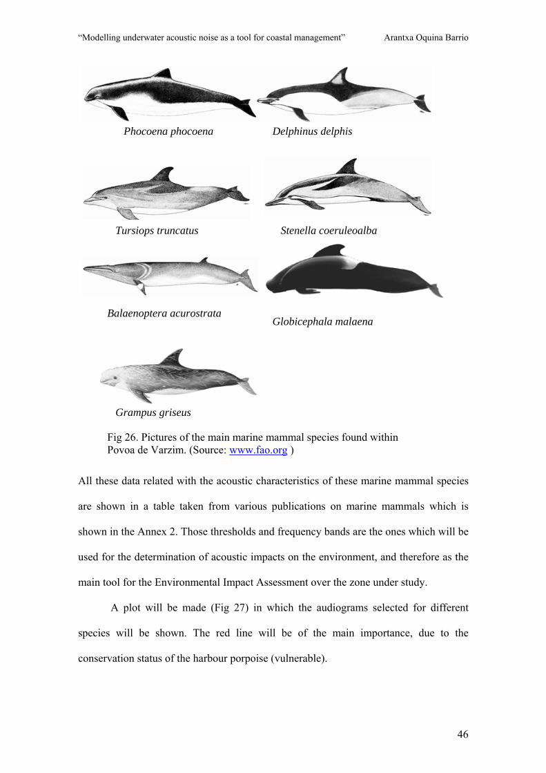
“Modelling underwater acoustic noise as a tool for coastal management” Arantxa Oquina Barrio
46
All these data related with the acoustic characteristics of these marine mammal species
are shown in a table taken from various publications on marine mammals which is
shown in the Annex 2. Those thresholds and frequency bands are the ones which will be
used for the determination of acoustic impacts on the environment, and therefore as the
main tool for the Environmental Impact Assessment over the zone under study.
A plot will be made (Fig 27) in which the audiograms selected for different
species will be shown. The red line will be of the main importance, due to the
conservation status of the harbour porpoise (vulnerable).
Phocoena phocoena Delphinus delphis
Tursiops truncatus Stenella coeruleoalba
Balaenoptera acurostrata Globicephala malaena
Grampus griseus
Fig 26. Pictures of the main marine mammal species found within Povoa de Varzim. (Source: www.fao.org )
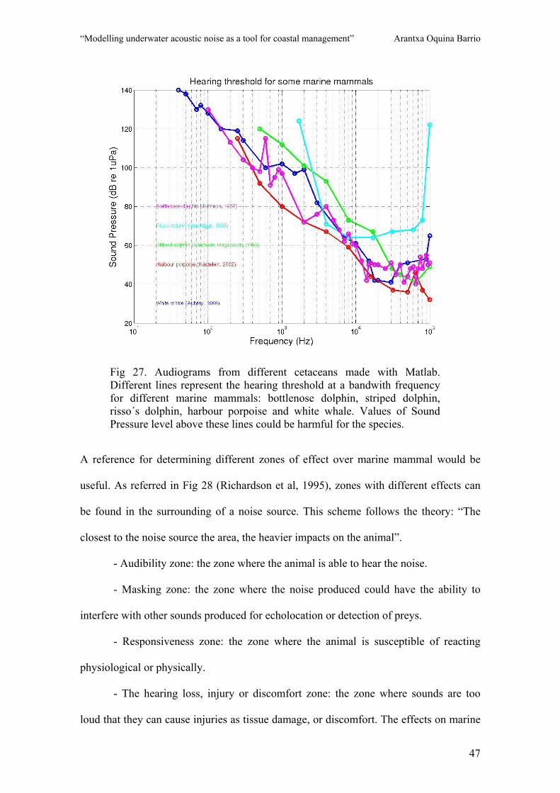
“Modelling underwater acoustic noise as a tool for coastal management” Arantxa Oquina Barrio
47
A reference for determining different zones of effect over marine mammal would be
useful. As referred in Fig 28 (Richardson et al, 1995), zones with different effects can
be found in the surrounding of a noise source. This scheme follows the theory: “The
closest to the noise source the area, the heavier impacts on the animal”.
- Audibility zone: the zone where the animal is able to hear the noise.
- Masking zone: the zone where the noise produced could have the ability to
interfere with other sounds produced for echolocation or detection of preys.
- Responsiveness zone: the zone where the animal is susceptible of reacting
physiological or physically.
- The hearing loss, injury or discomfort zone: the zone where sounds are too
loud that they can cause injuries as tissue damage, or discomfort. The effects on marine
Fig 27. Audiograms from different cetaceans made with Matlab. Different lines represent the hearing threshold at a bandwith frequency for different marine mammals: bottlenose dolphin, striped dolphin, risso´s dolphin, harbour porpoise and white whale. Values of Sound Pressure level above these lines could be harmful for the species.
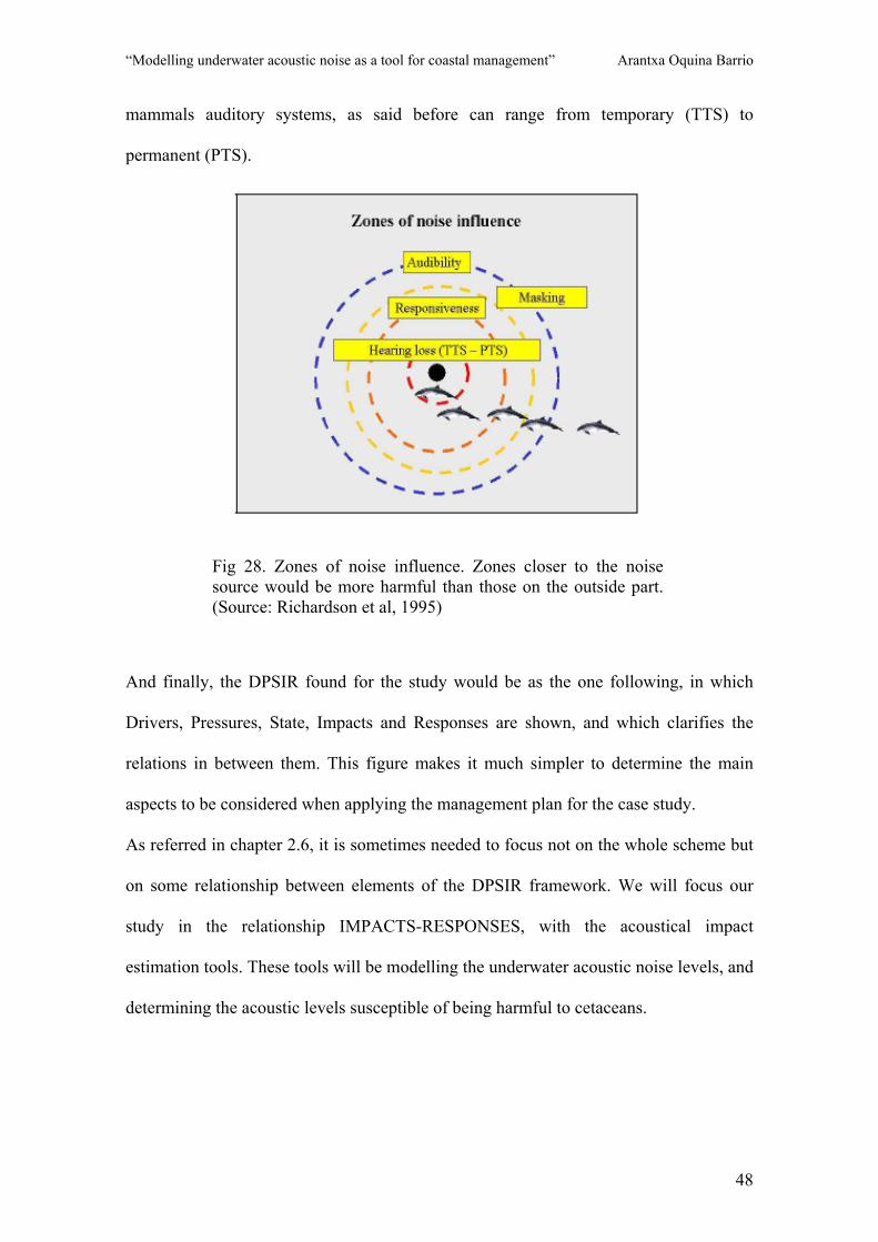
“Modelling underwater acoustic noise as a tool for coastal management” Arantxa Oquina Barrio
48
mammals auditory systems, as said before can range from temporary (TTS) to
permanent (PTS).
And finally, the DPSIR found for the study would be as the one following, in which
Drivers, Pressures, State, Impacts and Responses are shown, and which clarifies the
relations in between them. This figure makes it much simpler to determine the main
aspects to be considered when applying the management plan for the case study.
As referred in chapter 2.6, it is sometimes needed to focus not on the whole scheme but
on some relationship between elements of the DPSIR framework. We will focus our
study in the relationship IMPACTS-RESPONSES, with the acoustical impact
estimation tools. These tools will be modelling the underwater acoustic noise levels, and
determining the acoustic levels susceptible of being harmful to cetaceans.
Fig 28. Zones of noise influence. Zones closer to the noise source would be more harmful than those on the outside part. (Source: Richardson et al, 1995)

“Modelling underwater acoustic noise as a tool for coastal management” Arantxa Oquina Barrio
49
The acoustic data required for the model, could be obtained by the location of
hydrophones in strategic sites within the study area, in order to obtain a matrix with
different sound level values for running the model. In this case, these acoustic data
matrix will be randomly generated by the model as the real acoustical data from the
environment measured with hydrophones is still not available. A rms SPL for the source
will be selected and also the frequency band in which the source is supposed to be
emitting.
DPSIR FRAMEWORK SCHEME
DRIVER: ORED (Offshore Renewal Energy Device)
PRESSURE: Underwater acoustic noise
STATE: - Increased noise in
decibels - Decrease in number
of marine mammals
IMPACTS: ENVIRONMENTAL: Reduction of CO2
Increase in noise ECOLOGICAL:
Decrease in marine fauna (mammals) SOCIAL:
Increased jobs in wave energy Energy supply for population
ECONOMICAL: Improvement of Portuguese economical state
Reduction in electricity prices
RESPONSES: - Regulation, legislation - Monitoring, research
Impacts estimation tool Underwater acoustic noise levels. Threshold levels set for cetaceans.
Fig 29. Basic DPSIR framework scheme for the study site. There is an added element on this scheme, that functions as a link in between tha main elements, Impact estimation tools appears as a tool for facilitating the whole DPSIR framework comprehension.

“Modelling underwater acoustic noise as a tool for coastal management” Arantxa Oquina Barrio
50
6. MODELLING UNDERWATER NOISE LEVEL. OBTAINING SPATIAL
DISTRIBUTION MAPS.
Acoustic modelling will be carried out for cases combining three temperature profiles
during the year, considering several receiver depths, and a range of frequencies located
in the lower part of the waveband. As the noise generated by the real source is still
unknown, we used computer generated signal for carrying out acoustic modelling.
Three sources will be taken into account for the simplest case of study, one for
each Pelamis device. Wave front is supposed to come orthogonally to the line of
devices. This is the case that will be considered in this study, a more complicated case
will consist in the assumption of nine sources (corresponding to each converter of the
three devices in the plan) and wave front coming from any angle. The basic scheme for
both cases is shown in Fig 30.
Fig 30. Scheme of possible study cases. Case A is the most simple one, while case B is more complicated. Case A is including each device as a noise source, while B assumes each converter as a noise source. Wave front in case a comes at the same time to devices, creating a simultaneous signal from every noise source, while B has an angle, making the signals created to differ in time.
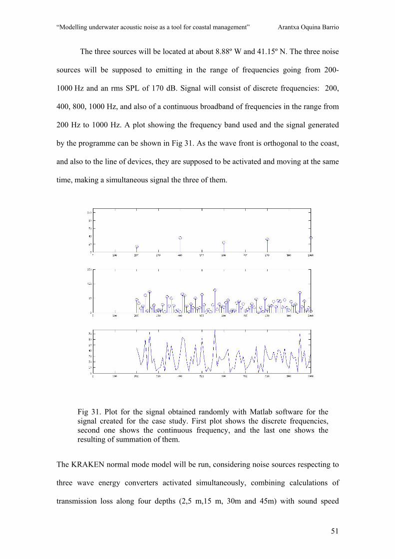
“Modelling underwater acoustic noise as a tool for coastal management” Arantxa Oquina Barrio
51
The three sources will be located at about 8.88º W and 41.15º N. The three noise
sources will be supposed to emitting in the range of frequencies going from 200-
1000 Hz and an rms SPL of 170 dB. Signal will consist of discrete frequencies: 200,
400, 800, 1000 Hz, and also of a continuous broadband of frequencies in the range from
200 Hz to 1000 Hz. A plot showing the frequency band used and the signal generated
by the programme can be shown in Fig 31. As the wave front is orthogonal to the coast,
and also to the line of devices, they are supposed to be activated and moving at the same
time, making a simultaneous signal the three of them.
The KRAKEN normal mode model will be run, considering noise sources respecting to
three wave energy converters activated simultaneously, combining calculations of
transmission loss along four depths (2,5 m,15 m, 30m and 45m) with sound speed
Fig 31. Plot for the signal obtained randomly with Matlab software for the signal created for the case study. First plot shows the discrete frequencies, second one shows the continuous frequency, and the last one shows the resulting of summation of them.
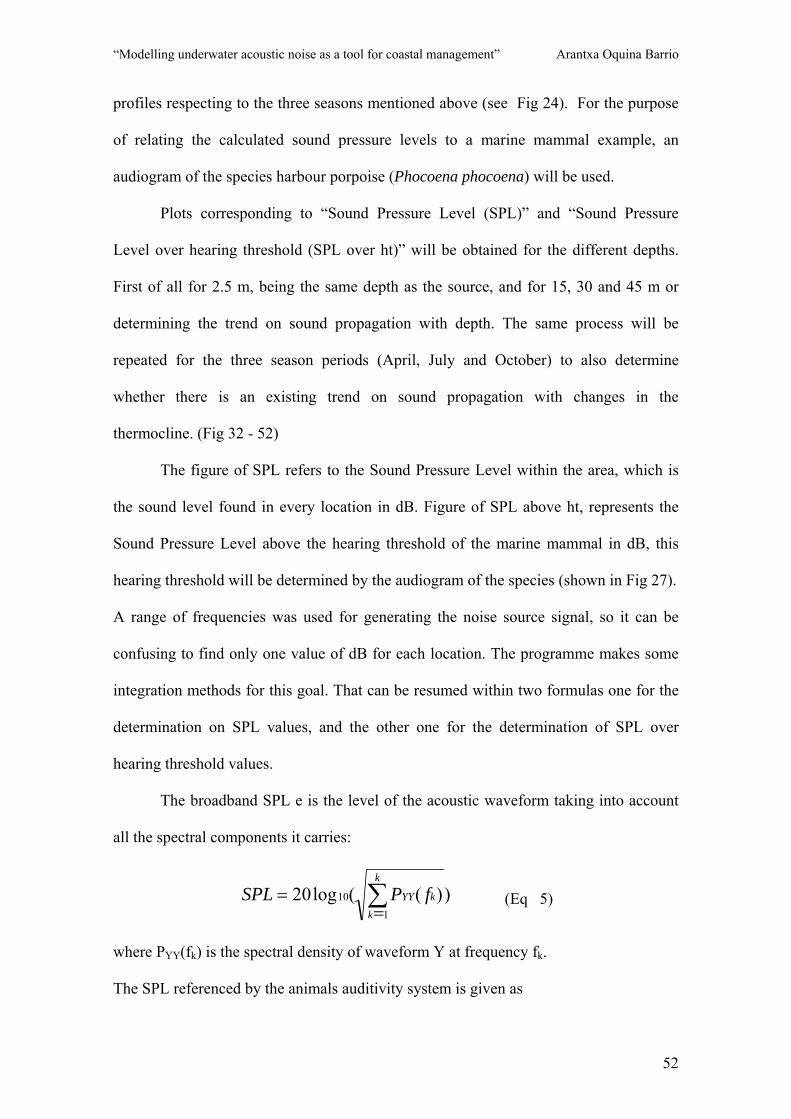
“Modelling underwater acoustic noise as a tool for coastal management” Arantxa Oquina Barrio
52
profiles respecting to the three seasons mentioned above (see Fig 24). For the purpose
of relating the calculated sound pressure levels to a marine mammal example, an
audiogram of the species harbour porpoise (Phocoena phocoena) will be used.
Plots corresponding to “Sound Pressure Level (SPL)” and “Sound Pressure
Level over hearing threshold (SPL over ht)” will be obtained for the different depths.
First of all for 2.5 m, being the same depth as the source, and for 15, 30 and 45 m or
determining the trend on sound propagation with depth. The same process will be
repeated for the three season periods (April, July and October) to also determine
whether there is an existing trend on sound propagation with changes in the
thermocline. (Fig 32 - 52)
The figure of SPL refers to the Sound Pressure Level within the area, which is
the sound level found in every location in dB. Figure of SPL above ht, represents the
Sound Pressure Level above the hearing threshold of the marine mammal in dB, this
hearing threshold will be determined by the audiogram of the species (shown in Fig 27).
A range of frequencies was used for generating the noise source signal, so it can be
confusing to find only one value of dB for each location. The programme makes some
integration methods for this goal. That can be resumed within two formulas one for the
determination on SPL values, and the other one for the determination of SPL over
hearing threshold values.
The broadband SPL e is the level of the acoustic waveform taking into account
all the spectral components it carries:
))((log201
10 ∑=
=k
k
kYY fPSPL (Eq 5)
where PYY(fk) is the spectral density of waveform Y at frequency fk.
The SPL referenced by the animals auditivity system is given as

“Modelling underwater acoustic noise as a tool for coastal management” Arantxa Oquina Barrio
53
))(
)((log20)(1
210 ∑=
=k
k k
kYYht
fHTfPspeciesSPL (Eq 6 )
where HT(fk) is the hearing threshold of the animal as a function of frequency.
(As all these variables are in linear scale we have to use the logarithmic transformation
to give results in dB).

“Modelling underwater acoustic noise as a tool for coastal management” Arantxa Oquina Barrio
54
Fig 32. SPL, April 2.5 m, Harbour porpoise Fig 33. SPL, April 15 m, Harbour porpoise
Fig 34. SPL, April 30 m, Harbour porpoise Fig 35. SPL, April 45 m, Harbour porpoise
Fig 36. SPL above ht, April 2.5 m, Harbour porpoise Fig 37. SPL above ht, April 15 m, Harbour porpoise

“Modelling underwater acoustic noise as a tool for coastal management” Arantxa Oquina Barrio
55
Fig 38. SPL above ht, April 30 m, Harbour porpoise Fig 39. SPL above ht, April 45 m, Harbour porpoise

“Modelling underwater acoustic noise as a tool for coastal management” Arantxa Oquina Barrio
56
Fig 40. SPL, July 2.5 m, Harbour porpoise Fig 41. SPL, July 15 m, Harbour porpoise
Fig 42. SPL, July 30 m, Harbour porpoise Fig 43. SPL, July 45 m, Harbour porpoise
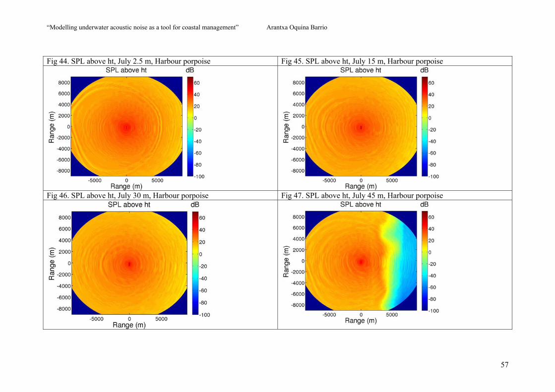
“Modelling underwater acoustic noise as a tool for coastal management” Arantxa Oquina Barrio
57
Fig 44. SPL above ht, July 2.5 m, Harbour porpoise Fig 45. SPL above ht, July 15 m, Harbour porpoise
Fig 46. SPL above ht, July 30 m, Harbour porpoise Fig 47. SPL above ht, July 45 m, Harbour porpoise
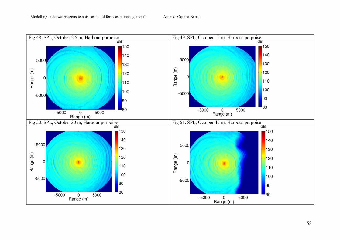
“Modelling underwater acoustic noise as a tool for coastal management” Arantxa Oquina Barrio
58
Fig 48. SPL, October 2.5 m, Harbour porpoise Fig 49. SPL, October 15 m, Harbour porpoise
Fig 50. SPL, October 30 m, Harbour porpoise Fig 51. SPL, October 45 m, Harbour porpoise
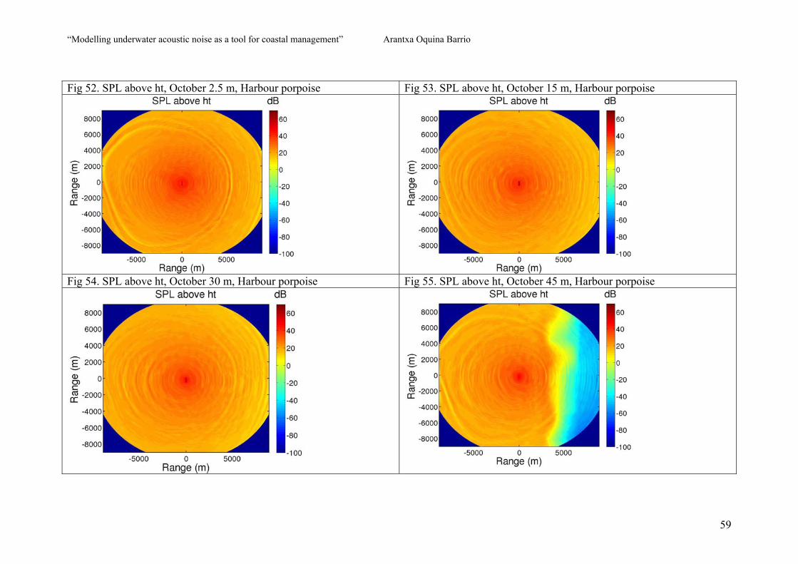
“Modelling underwater acoustic noise as a tool for coastal management” Arantxa Oquina Barrio
59
Fig 52. SPL above ht, October 2.5 m, Harbour porpoise Fig 53. SPL above ht, October 15 m, Harbour porpoise
Fig 54. SPL above ht, October 30 m, Harbour porpoise Fig 55. SPL above ht, October 45 m, Harbour porpoise
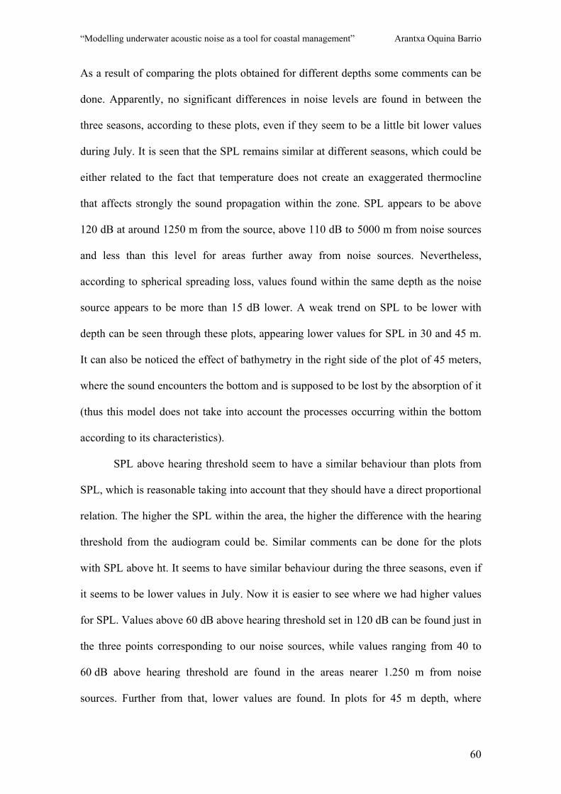
“Modelling underwater acoustic noise as a tool for coastal management” Arantxa Oquina Barrio
60
As a result of comparing the plots obtained for different depths some comments can be
done. Apparently, no significant differences in noise levels are found in between the
three seasons, according to these plots, even if they seem to be a little bit lower values
during July. It is seen that the SPL remains similar at different seasons, which could be
either related to the fact that temperature does not create an exaggerated thermocline
that affects strongly the sound propagation within the zone. SPL appears to be above
120 dB at around 1250 m from the source, above 110 dB to 5000 m from noise sources
and less than this level for areas further away from noise sources. Nevertheless,
according to spherical spreading loss, values found within the same depth as the noise
source appears to be more than 15 dB lower. A weak trend on SPL to be lower with
depth can be seen through these plots, appearing lower values for SPL in 30 and 45 m.
It can also be noticed the effect of bathymetry in the right side of the plot of 45 meters,
where the sound encounters the bottom and is supposed to be lost by the absorption of it
(thus this model does not take into account the processes occurring within the bottom
according to its characteristics).
SPL above hearing threshold seem to have a similar behaviour than plots from
SPL, which is reasonable taking into account that they should have a direct proportional
relation. The higher the SPL within the area, the higher the difference with the hearing
threshold from the audiogram could be. Similar comments can be done for the plots
with SPL above ht. It seems to have similar behaviour during the three seasons, even if
it seems to be lower values in July. Now it is easier to see where we had higher values
for SPL. Values above 60 dB above hearing threshold set in 120 dB can be found just in
the three points corresponding to our noise sources, while values ranging from 40 to
60 dB above hearing threshold are found in the areas nearer 1.250 m from noise
sources. Further from that, lower values are found. In plots for 45 m depth, where

“Modelling underwater acoustic noise as a tool for coastal management” Arantxa Oquina Barrio
61
bottom is supposed to be found, the right side of the plots show again the interaction
with the bottom, and then show values below zero, as no sound is found for the
programme within the bottom sea floor.
There is a little trend in higher values (either in SPL and SPL above ht) to be
dislocated to the left, which could be related to the presence of higher depth to
propagate. That could mean that sound propagates better in higher depths, according to
the absence of bottom loss.

“Modelling underwater acoustic noise as a tool for coastal management” Arantxa Oquina Barrio
62
7. VALIDATION OF THE MODEL.
Plots for facilitating this part are obtained for the validation of the model. Behavioural
effects are difficult to model, while effects based on the hearing range of marine
mammals are so much easier predictable. Thus, plots for “disturbance”, “audibility”,
and “4-6 dB TTS”, and “4-6 dB TTS + 10 dB”. The figure of audibility shows those
points where the marine mammal is susceptible of perceiving noise. For the obtaining of
this plot, values of 20 dB above the audiogram will be taken into account. The figure of
disturbance (for any cetacean considered) takes the main value of 120 dB instead, and
all the values over this one will be considered for the obtaining of the plot. Finally,
a temporary injury zone will be determined by the obtaining of the 4-6 dB TTS plot.
This plot is obtained by assuming a noise source emitting 30 dB louder and considering
the cetacean audiogram (Fig 27). The last plot obtained, would be an extreme case in
which the sources are added even 10 dB more, and is calculated the same way as the
previous plot.
In the previous plots for SPL and SPL above hearing threshold it was quite
difficult to distinguish the areas where effects over marine mammals where susceptible
to be found. All these plots make it easier to determine which is the extension of the
area susceptible of being affected by the different effects defined for its calculation.
The plots obtained show basically the areas where the cetaceans would be affected by
the noise level existing. They show the distances from the sources where cetacean are
susceptible of suffering because of noise propagation.
“Modelling underwater acoustic noise as a tool for coastal management” Arantxa Oquina Barrio
63
Fig 56. Disturbance, April 2.5 m, Harbour porpoise Fig 57. Disturbance, April 15 m, Harbour porpoise
Fig 58. Disturbance, April 30 m, Harbour porpoise Fig 59. Disturbance, April 45 m, Harbour porpoise
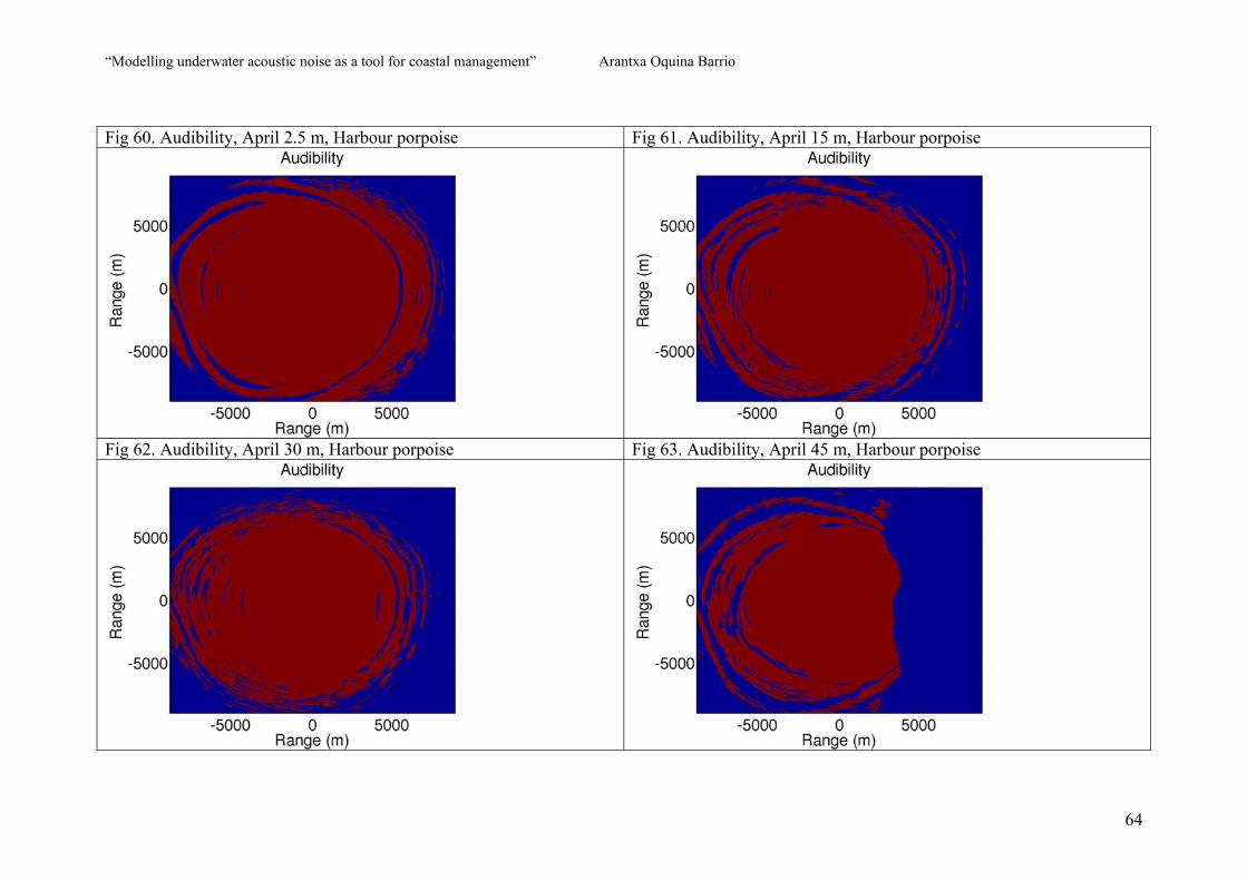
“Modelling underwater acoustic noise as a tool for coastal management” Arantxa Oquina Barrio
64
Fig 60. Audibility, April 2.5 m, Harbour porpoise Fig 61. Audibility, April 15 m, Harbour porpoise
Fig 62. Audibility, April 30 m, Harbour porpoise Fig 63. Audibility, April 45 m, Harbour porpoise

“Modelling underwater acoustic noise as a tool for coastal management” Arantxa Oquina Barrio
65
Fig 64. 4-6 dB TTS, April 2.5 m, Harbour porpoise Fig 65. 4-6 dB TTS, April 15 m, Harbour porpoise
Fig 66. 4-6 dB TTS, April 30 m, Harbour porpoise Fig 67. 4-6 dB TTS, April 45 m, Harbour porpoise
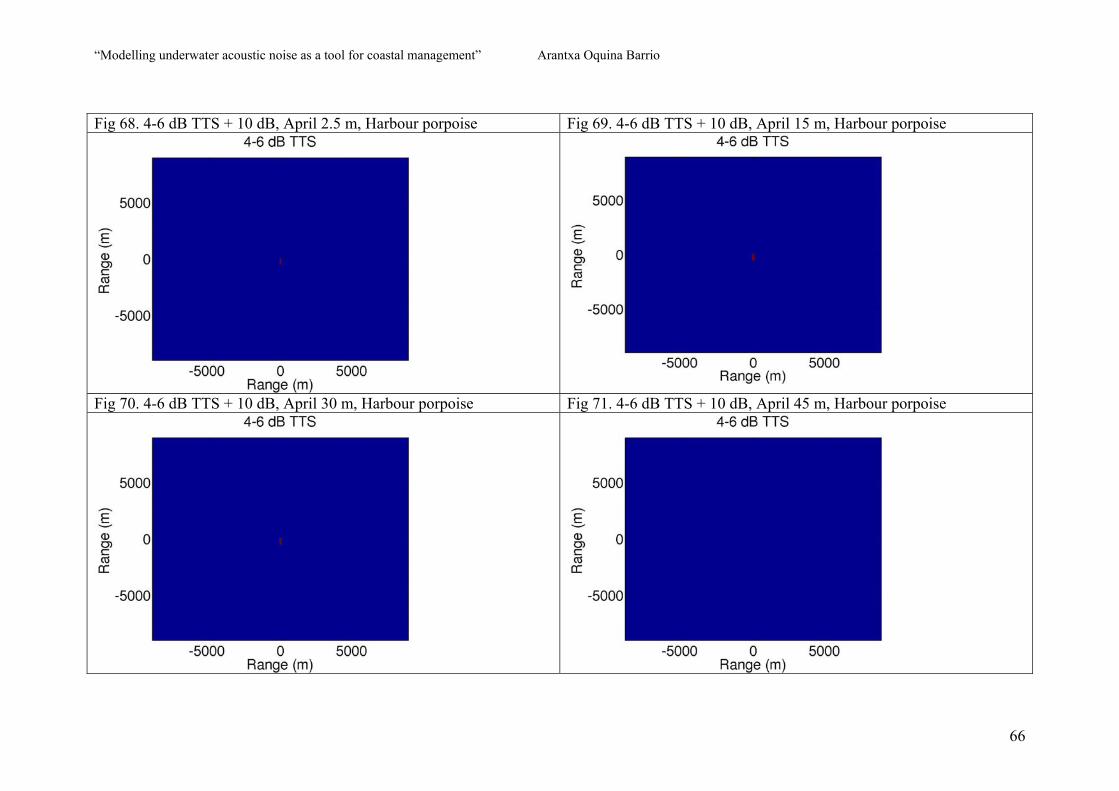
“Modelling underwater acoustic noise as a tool for coastal management” Arantxa Oquina Barrio
66
Fig 68. 4-6 dB TTS + 10 dB, April 2.5 m, Harbour porpoise Fig 69. 4-6 dB TTS + 10 dB, April 15 m, Harbour porpoise
Fig 70. 4-6 dB TTS + 10 dB, April 30 m, Harbour porpoise Fig 71. 4-6 dB TTS + 10 dB, April 45 m, Harbour porpoise

“Modelling underwater acoustic noise as a tool for coastal management” Arantxa Oquina Barrio
67
Fig 72. Disturbance, July 2.5 m, Harbour porpoise Fig 73. Disturbance, July 15 m, Harbour porpoise
Fig 74. Disturbance, July 30 m, Harbour porpoise Fig 75. Disturbance, July 45 m, Harbour porpoise

“Modelling underwater acoustic noise as a tool for coastal management” Arantxa Oquina Barrio
68
Fig 76. Audibility, July 2.5 m, Harbour porpoise Fig 77. Audibility, July 15 m, Harbour porpoise
Fig 78. Audibility, July 30 m, Harbour porpoise Fig 79. Audibility, July 45 m, Harbour porpoise

“Modelling underwater acoustic noise as a tool for coastal management” Arantxa Oquina Barrio
69
Fig 80. 4-6 dB TTS, July 2.5 m, Harbour porpoise Fig 81. 4-6 dB TTS, July 15 m, Harbour porpoise
Fig 82. 4-6 dB TTS, July 30 m, Harbour porpoise Fig 83. 4-6 dB TTS, July 45 m, Harbour porpoise

“Modelling underwater acoustic noise as a tool for coastal management” Arantxa Oquina Barrio
70
Fig 84. 4-6 dB TTS + 10 dB, July 2.5 m, Harbour porpoise Fig 85. 4-6 dB TTS + 10 dB, July 15 m, Harbour porpoise
Fig 86. 4-6 dB TTS + 10 dB, July m, Harbour porpoise Fig 87. 4-6 dB TTS + 10 dB, July 45 m, Harbour porpoise
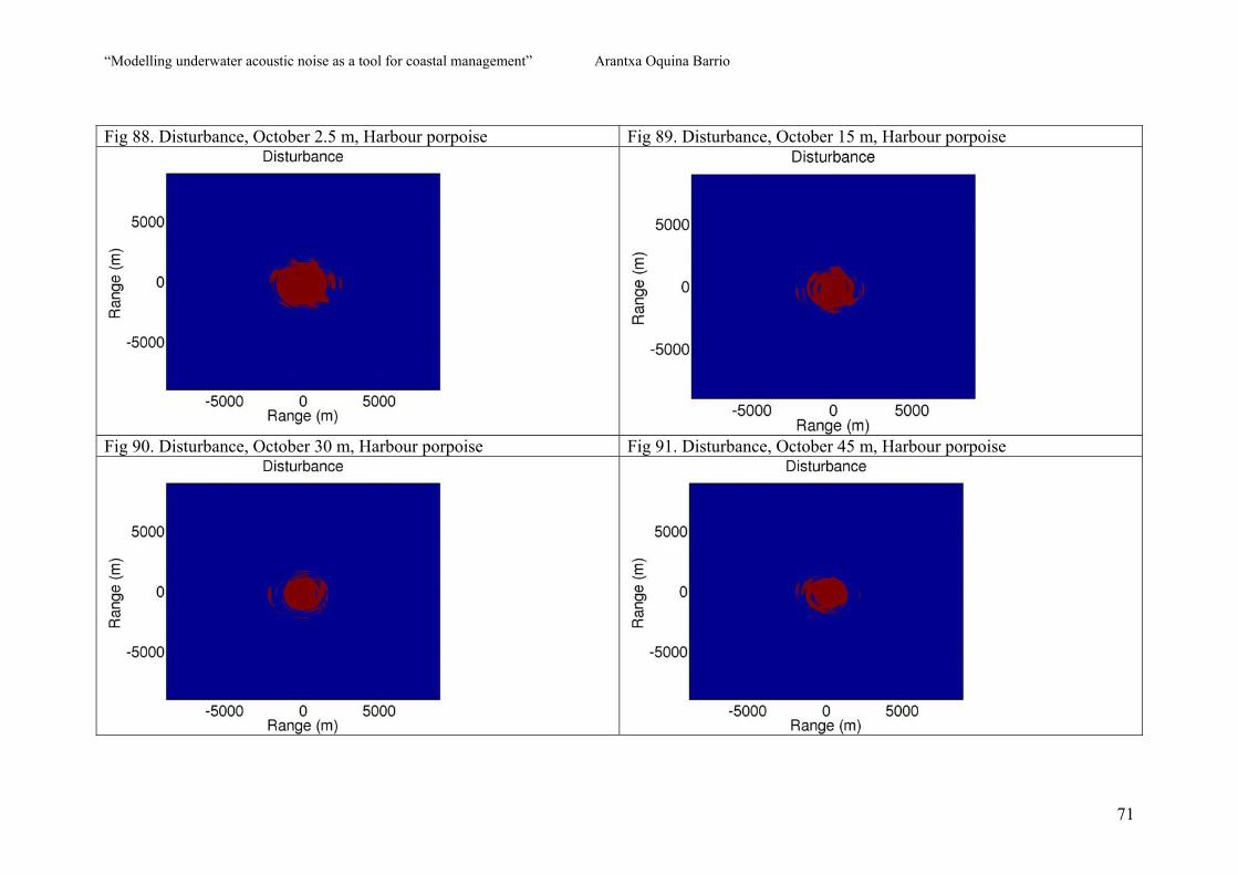
“Modelling underwater acoustic noise as a tool for coastal management” Arantxa Oquina Barrio
71
Fig 88. Disturbance, October 2.5 m, Harbour porpoise Fig 89. Disturbance, October 15 m, Harbour porpoise
Fig 90. Disturbance, October 30 m, Harbour porpoise Fig 91. Disturbance, October 45 m, Harbour porpoise

“Modelling underwater acoustic noise as a tool for coastal management” Arantxa Oquina Barrio
72
Fig 92. Audibility, October 2.5 m, Harbour porpoise Fig 93. Audibility, October 15 m, Harbour porpoise
Fig 94. Audibility, October 30 m, Harbour porpoise Fig 95. Audibility, October 45 m, Harbour porpoise

“Modelling underwater acoustic noise as a tool for coastal management” Arantxa Oquina Barrio
73
Fig 96. 4-6 dB TTS, October 2.5 m, Harbour porpoise Fig 97. 4-6 dB TTS, October 15 m, Harbour porpoise
Fig 98. 4-6 dB TTS, October 30 m, Harbour porpoise Fig 99. 4-6 dB TTS, October 45 m, Harbour porpoise
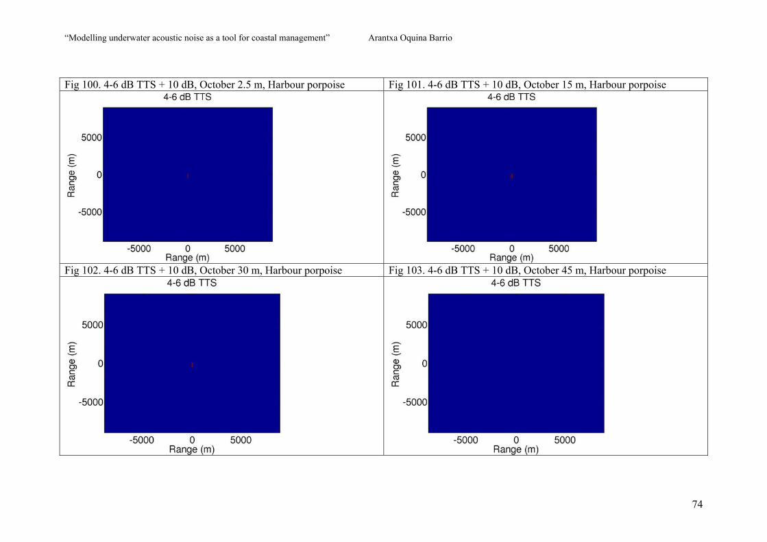
“Modelling underwater acoustic noise as a tool for coastal management” Arantxa Oquina Barrio
74
Fig 100. 4-6 dB TTS + 10 dB, October 2.5 m, Harbour porpoise Fig 101. 4-6 dB TTS + 10 dB, October 15 m, Harbour porpoise
Fig 102. 4-6 dB TTS + 10 dB, October 30 m, Harbour porpoise Fig 103. 4-6 dB TTS + 10 dB, October 45 m, Harbour porpoise
“Modelling underwater acoustic noise as a tool for coastal management” Arantxa Oquina Barrio
75
There is always a general trend in the plots obtained to have reducing areas with depth.
The plots obtained do not seem to have a significant variation along the year, having
similar shapes for every same plot at the same depth.
Disturbance plots show an area of about 1,5 km ratio from the source, which
gets a little smaller with depth.
The areas found for audibility appear to be much wider, reaching the ratio of
5 km from the noise source.
Areas for the effects of up to 6 dB TTS, seem to reach the 2,5 km ratio, which is
a bigger ratio than the one found for the disturbance area. That means, that if the source
where louder, it would mean a real extension in the area where actually injuries could be
affecting the marine mammals.
For the extreme situations simulation, it appears to be only significant in the
noise source points.
All this plots represent the values over the reference set, that would mean that
they represent those areas where the answer to the question “Does the noise exceed the
threshold within the zone?” is positive, and so, a reapproachment of the project should
be carried on, or some management actions has to be applied.

“Modelling underwater acoustic noise as a tool for coastal management” Arantxa Oquina Barrio
76
8. DISCUSSION:
Every developing plan occurring within the coast affects many social, economical and
ecological variables that have to be taken into account while managing any of these
programmes. A correct EIA and management are required for the evaluation of any
plan.
New reliable tools need to be found to give the manager the ability of predicting
impacts and facilitate how to measure and manage these environmental impacts. For the
case of appearing of underwater acoustic noise impact onto the ocean, it converts the
objective of managing into a real problem. As it is difficult to measure and evaluate the
damages that it could cause over the environment as well as the propagation paths and
transmission loss that noise suffers within the ocean. Modelling the underwater acoustic
noise would be a useful tool for determining whether management actions should be
applied within the zone, and how to implement them.
The main reason why sound requires a further study within the ocean is because
its attenuation can be so weak that it can travel along long distances, with the added fact
of being the most important sense for some marine animals as cetaceans.
The introduction of noise into the ocean by installation of OREDs is clearly
a serious issue for marine mammals, and it needs to be correctly analysed and evaluated,
taking into account that even installing is already taking place.
Modelling the underwater acoustic noise will firstly give the manager the ability
of predicting expected noise values in every point of the water column, and thus giving
him the opportunity of creating noise level maps. These noise level maps will give an
intuitive idea of how the sound is transmitted within the study area. This would be
a complex end expensive task if we had to make them with experimental data, because
of the technology required and the inaccessibility of the mean. Afterwards, maps
“Modelling underwater acoustic noise as a tool for coastal management” Arantxa Oquina Barrio
77
showing the areas susceptible of having any effect on marine mammals are easy to
obtain, by comparison of sound level values with audiograms giving hearing thresholds
for marine mammals. They facilitate a lot the determination of impact areas. After
determining the spatial distribution of underwater acoustic noise and comparison of
sound level values with thresholds set for marine mammals, it could also be appropriate
to make a gradation map with distance, where zones of maximum, medium and
minimum effects can be shown. This could be a good tool for determining the areas
where more or less protection or management is needed.
For the determination of the impacts on marine mammals, behavioural and
physiological effects can be studied such as hearing loss. Predicting hearing loss
appears to be a complex task. Nevertheless, studies are being carried on in order to give
more and more precise information about hearing loss in marine mammals. Values for
temporary hearing loss (TTS – Temporary Threshold Shift) and (PTS – Permanent
Threshold Shift) are given for different species on marine mammals. Exposure for long
periods to TTS is susceptible to convert those levels into PTS. Thus, it is important to
know the duration of the noise, which in this case is not possible as no real information
about the noise source is still available.
The results obtained by the model determine whether the sound pressure levels
obtained are loud enough to make any disturbance to the marine mammals existing in
the zone. After running the model, the results have shown that they are able to give
precise predicted areas with different effects over marine mammals. These simulated
scenarios give also the possibility of experimenting possible effects and determining
effect areas if the source is louder or quieter, for example, as we are allowed to change
any source or environmental characteristic within the model. Also, it can be run plenty
of times to study the best way of implementing any plan

“Modelling underwater acoustic noise as a tool for coastal management” Arantxa Oquina Barrio
78
PROPOSED STRATEGIES ON OCEAN NOISE MANAGEMENT.
A. SAFE EXPOSURE LEVELS - Establishment of a particular noise level, such as TTS, PTS or others.
B. MITIGATION MEASURES AND THEIR SHORTCOMINGS. - SAFETY ZONES: establishment of visual safety zones, where observers
determine the presence of cetaceans and temporarily can shut down or reduce
the power of noise source.
- “RAMP-UP” or “SOFT-START”: Consisting in the gradually introduction
of noise into the environment, assuming the possibility of the animal to move
away without any significant impacts. (still not proven)
C. PRECAUTION IN MANAGEMENT. - Setting of precautionary steps for preventing the effects and helping
protection. First by increasing the protection before irreversible damage is
done. Secondly, by distancing noise events from biologically important areas
or concentrations of cetaceans.
D. SOURCE MODIFICATION. - Changing the noise source characteristics, and building quieter noise
sources.
E. SEASONAL AND GEOGRAPHIC EXCLUSIONS. - Distancing noise events from important biological areas, or either manage
seasonal functioning.

“Modelling underwater acoustic noise as a tool for coastal management” Arantxa Oquina Barrio
79
PROPOSED STRATEGIES ON OCEAN NOISE MANAGEMENT.
F. MARINE PROTECTED AREAS (MPAs) - Creation of zones, that if well-managed, offer the most effective means to
protect cetaceans and their habitat (regulation over the entire ecosystem),
from noise and any other anthropogenic stressors.
G. REDUCTION IN NOISE PRODUCING ACTIVITIES. - Reducing noise-production activities by maximizing the results obtained for
every trip or exploration, and by sharing data and results obtained in order to
minimize the noise sources entering the ocean.
H. MONITORING - MONITORING AND REPORTING: essential parts of management actions.
Further studies on cetacean strandings and mortalities for appropriate
thresholds/impacts determination. Usage of Passive Acoustic Monitoring
(PAM) to detect presence of cetaceans, and to assess sources and levels of
anthropogenic noise Detection on how noise affects distribution and
vocalization of cetaceans.
Table 3. Proposed strategies on ocean noise management. Table created from Weilgart, 2007.

“Modelling underwater acoustic noise as a tool for coastal management” Arantxa Oquina Barrio
80
Some strategies for ocean noise management were described by Weilgart, which are
shown in Table 3. It will be discussed which of them are applicable in this case. Safe
exposure levels (TTS, PTS, disturbance, audibility), were already used for the
determination of the areas susceptible of causing any damage to cetaceans. Concerning
the mitigation measures, it is unexpected that the power of the noise source could be
gradually introduced or reduced in some moments, as it is activated by the wave motion
and it starts functioning at the rms SPL at the moment when it is installed and activated
by the waves, and can not be externally regulated or gradually increased. Precaution
management could be done, trying to create legislations and protection figures that
include the effects of noise before the installation of all these kind of devices. Source
modification could be done by the engineering enterprise in order to minimize the
impacts made by the noise, maximizing the energy provided. Seasonal and geographic
exclusions could be a possible action if cetacean and their behaviour within the zone
were further studied to determine if there is a period where their presence is
concentrated. In this case, the device could be retired within this period. Even though,
economically aspects of device transport and reinstallation should be taken into account
in order to study the profitability of this action. The creation of MPAs should be done
before the installation of the device, because in this case it can not be assumed.
Reduction of noise producing activities could be done by maximizing the relation
energy obtained/noise produced. Finally, monitoring will always be important during
the planning, installing or even decommissioning phase of the plan, in order to make
a reliable report on the species within the zone and their behaviour in the presence of
noise.
It is important for the manager to use modelling only as a tool and not forget the
rest of the DPSIR framework scheme. It is important to integrate the results obtained

“Modelling underwater acoustic noise as a tool for coastal management” Arantxa Oquina Barrio
81
with this study but give the appropriate weight to each of the elements within the
scheme before the whole plan decision-making.
There are many uncertainties involving this study:
- Lack of in-situ measurements to give information about noise source real
characteristics (rms SPL, frequencies, duration of signals)
- Data for hearing thresholds in marine mammals has still to be studied further
to reassure the limits over which real effects can be generated. It still exist
much uncertainty about cetacean hearing and the ways to measure it.
- Data for hearing thresholds were not found for every species existing within
the study area.
- There are no concrete existing laws on underwater acoustic noise produced
by off-shore devices. Management over these plans have to be done then by
the usage of policies implying protective figures over some of the marine
mammals existing within the zone. It is important to consider underwater
acoustic noise as a pollutant, with no boundaries, and to highlight the
necessity of promoting its prevention, reduction and control.
- The case considered has some limitations as the wave front is orthogonal to
the coast and we are only assuming three noise sources in order to simplify
the example.
- Effects of natural underwater acoustic noise were not added to the noise
levels obtained, also can not be forgotten.
“Modelling underwater acoustic noise as a tool for coastal management” Arantxa Oquina Barrio
82
9. CONCLUSIONS AND RECOMMENDATIONS:
It appears to be demonstrated that the viability of modelling underwater acoustic noise
and the procedure followed as a tool for coastal management can answer the question
“Does the noise exceed the threshold within the zone?” It allows the manager to
determine the areas susceptible of having negative impacts to the animals, and thus, be
able to decision-making.
Results obtained from this study give evidence that the use of tools, such as
modelling physical properties related with some projects, need to be integrated into
management for improving decision-making processes over renewal energy projects.
Also the same needs to be done for setting guidelines, which can be used for future
creation of directives and legislation, as they give a reliable simulated scenario which
can allow the manager to have information that, without modelling would be practically
inaccessible. This study made a simple example of the way modelling can help in
determining the damaging effects that a project in a hostile medium such as the ocean
can have into marine organisms.
Nevertheless, the case study is still very new that reliable information was still
not available, and it is shown as a reference/example of what can be done in the future
research for management. We only intended to show an example of how the current
existing tools can be applied to perform a correct management process of the increasing
use of off-shore devices.
As recommendations after the carrying out of this study:
- Study over the zones where OREDs are planned to be installed should be
done in order to place them. If possible, it should be placed in those places
where less marine life and impacts exist. However, this should be done even
“Modelling underwater acoustic noise as a tool for coastal management” Arantxa Oquina Barrio
83
before installing the device, which is not possible in this study case as the
device is already installed.
- Further study over marine mammals and their behavioural and hearing
responses to different types of noise should be done, and data should be put
in together for determining reliable thresholds within the scientific
community.
- There is a need of a correct DPSIR framework scheme in order to use it as a
guide for coastal management decision-making. This importance resides in
the fact that sometimes there is a lack in between the different elements of
the scheme and difficulties appear during the decision making process. That
is the reason why it is important to determine the appropriate tools for
relating the elements and making the links in between them more
comprehensible.
- Introduction of available advanced technology tools should be facilitated to
clarify as many of the DPSIR framework schemes as possible.
- Real data should be obtained for noise source and environment to determine
the real effects of ORED installation within the study area. Also the
complete case study should be taken into account for the determination of
effects under every possible situation.
- Transboundary and international policies should be created for underwater
acoustic noise introduction into the ocean, as well as for ORED installation.
That is of an imminent necessity as ORED are already being installed along
the worldwide coasts.
“Modelling underwater acoustic noise as a tool for coastal management” Arantxa Oquina Barrio
84
- Even though the model has been demonstrated to have reliable results, the
collection of real in-situ data by hydrophones would always be
recommended to validate the model.
- This study is considering the operating phase underwater acoustic noise,
though it would be recommended to consider the noise produced during the
installation and decommissioning phases.
- It would also be interesting to determine the cumulative effects of the
underwater acoustic noise introduced by OREDs, as their number is
increasing.
- Wide-ranging perspective, adaptable monitoring and research based on our
best understanding of coastal environment would be needed, for the
installation and remaining of every ORED located into the coast.
Different types of OREDs have been already set into our coasts, but creating a correct
management procedure before their installation is a complete necessity, as there is an
evidence that they are actually necessary for current energetic society requirements.
“Modelling underwater acoustic noise as a tool for coastal management” Arantxa Oquina Barrio
85
Bibliography
- BUCKINGHAM, M.J. “Ocean-acoustic propagation models” Journal acoustique
(1992) 223-287.
- DELPHIS. 2004. Informe sobre Varamientos de Cetáceos y Tortugas Marinas
en la Provincia de Cádiz. Ecologistas en Acción. Septiembre. 21 pp.
- ENS. “Noisy, acid oceans increasingly harmful to whales”. Press release, issued
December 3rd 2008.
- EUROPEAN COMMISSION RESEARCH NEWS, 2004. “`Calming´influence-
European noise pollution network”. 26 October 2004.
(http://ec.europa.eu/research/transport/news/article_1608_en.html)
- GILL, A.B. “Offshore renewable energy: ecological implications of generating
electricity in the coastal zone” Journal of applied Ecology, 2005. 42, 605-615.
- HASTINGS, M.C. 2008. “Coming to terms with the effects of ocean noise on
marine animals”. Acoustics today, volume 4, issue 2. April 2008. pp 22-33.
- JACOBSON, S., JOHNSON, A. “The diffusion of renewable energy
technology: an analytical framework and key issues for research”. Elsevier,
Energy Policy 28 (2000) 625-640.
- JENSEN, F., KUPERMAN, W., PORTER, M. and SCHMIDT. “Computational
Ocean Acoustics“. American institute of Physics, New Cork, 1994.
- KAKUTA et al. “Review of Underwater Acoustic Sources and Evolution of
Environmental Policy on Marine Artificial Sounds” IEEE, 2004. pp 1706-1709.
- KELLY, C., GLEGG, G.A., SPEEDIE, C.D. “Management of marine wildlife
disturbance” ELSEVIER, 2004. Ocean and coastal management 47 (2009) 1 19.
- KRISTENSEN, P. “The DPSIR Framework” UNEP headquarters, Nairobi,
Kenya. September 2004.

“Modelling underwater acoustic noise as a tool for coastal management” Arantxa Oquina Barrio
86
- LOPEZ, A., SAGARMINAGA R. y LOSADA S. 2003. “Cetáceos en un Océano
Degradado: el Caso Español”. Greenpeace y Sociedad Española de Cetáceos.
Madrid – España. Mayo. 32 pp.
- MALDONADO, D., ALCALÁ, V. “Bioacústica en Cetáceos”. Facultad de
Ciencias del Mar de la Universidad de Cádiz. Fundación Bitácora. 1996
Disponible en http://www.terra.es/personal/fbitacora/Bio.htm (Consulted in
December 2004).
- MANGHI, M., PAVAN, G. “Taking a picture of underwater sounds” Accobams
kit for Field Cetacean Research, September 2002.
- MMPA 1997. Marine Mammal Commission Annual Report to Congress.
- NATIONAL RESEARCH SOUNCIL. 2005. “Marine Mammal Populations and
Ocean Noise: determining When Noise Causes Biologically Significant Effects”.
Free executive summary at http://www.nap.edu/catalog/11147.html
- NATIONAL RESEARCH COUNCIL. 2003. “Ocean Noise and Marine
Mammals”. The National Academies Press. Washington D.C. – E.E.U.U.
- NEDWELL, J.R., EDWARDS, B. TURNPENNY, A.W.H, GORDON, J. “Fish
and marine mammal audiograms: a summary of available information”.
Subacoustec report ref. 534R0214, submitted to Chevron Texaco Ltd, 278 pp.
- PREISIG, J. “Acoustic Propagation Considerations for Underwater Acoustic
Comunications Network Development”. Proceedings of the 1st ACM
international Workshop on Underwater Networks. September, 2006. Los
Angeles, California.
- REID, J.B, EVANS, P. and NORTHRIDGE, S.P “Atlas of Cetacean distribution
in north-west european waters” Joint Nature Conservation Comitee, 2003.

“Modelling underwater acoustic noise as a tool for coastal management” Arantxa Oquina Barrio
87
- RICHARDSON et al. 1995. “Marine Mammals and Noise”. Academic Press.
San Diego – E.E.U.U.
- RODRIGUES, L. “Wave power conversion systems for electrical energy
production”. Nova university of Lisbon.
- THE ECONOMIST TECHNOLOGY QUARTERLY. 2008. “The coming
wave”. Press release, issued June 7th 2008.
- THOMSEN, F. , LÜDEMAN, K. , KAFEMAN, R. And PIPER, W. “Effects of
offshore wind farm noise on marine mammals and fish” COWRIE ltd, July,
2006.
- URICK, R.J. “Principles of underwater sound” Ed McGrawHill, New York,
1983.
- WEILGART, L.S. “The impacts of anthropogenic ocean noise on cetaceans and
implications for management” NRC Research Press Canada, 2007. 85: 1091-
1116.
- WILHELMSSON, D., MALM, T., AND ÖHMAN, M.C. “The influence of off-
shore windpower on demersal fish”. ICES Journal of Marine Science, 63:775-
784, 2006.

“Modelling underwater acoustic noise as a tool for coastal management” Arantxa Oquina Barrio
88
ANNEX 1 The following graphs shows the different audiograms found for the marine mammals
existing in the zone under study. Source: Nedwell et al 2004, “Fish and marine
mammals audiograms”.
Bottlenose dolphin (Tursioups truncatus)
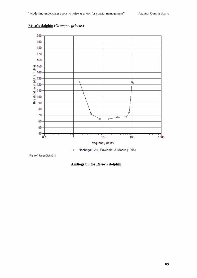
“Modelling underwater acoustic noise as a tool for coastal management” Arantxa Oquina Barrio
89
Risso’s dolphin (Grampus griseus)

“Modelling underwater acoustic noise as a tool for coastal management” Arantxa Oquina Barrio
90
Striped dolphin (Stenella coeruleoalba)

“Modelling underwater acoustic noise as a tool for coastal management” Arantxa Oquina Barrio
91
Harbour porpoise (Phocoena phocoena)
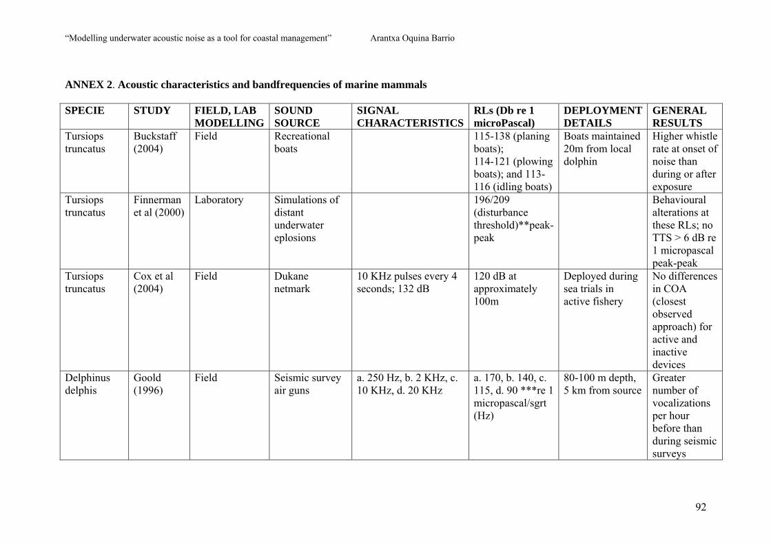
“Modelling underwater acoustic noise as a tool for coastal management” Arantxa Oquina Barrio
92
ANNEX 2. Acoustic characteristics and bandfrequencies of marine mammals
SPECIE STUDY FIELD, LAB MODELLING
SOUND SOURCE
SIGNAL CHARACTERISTICS
RLs (Db re 1 microPascal)
DEPLOYMENT DETAILS
GENERAL RESULTS
Tursiops truncatus
Buckstaff (2004)
Field Recreational boats
115-138 (planing boats); 114-121 (plowing boats); and 113-116 (idling boats)
Boats maintained 20m from local dolphin
Higher whistle rate at onset of noise than during or after exposure
Tursiops truncatus
Finnerman et al (2000)
Laboratory Simulations of distant underwater eplosions
196/209 (disturbance threshold)**peak-peak
Behavioural alterations at these RLs; no TTS > 6 dB re 1 micropascal peak-peak
Tursiops truncatus
Cox et al (2004)
Field Dukane netmark
10 KHz pulses every 4 seconds; 132 dB
120 dB at approximately 100m
Deployed during sea trials in active fishery
No differences in COA (closest observed approach) for active and inactive devices
Delphinus delphis
Goold (1996)
Field Seismic survey air guns
a. 250 Hz, b. 2 KHz, c. 10 KHz, d. 20 KHz
a. 170, b. 140, c. 115, d. 90 ***re 1 micropascal/sgrt (Hz)
80-100 m depth, 5 km from source
Greater number of vocalizations per hour before than during seismic surveys

“Modelling underwater acoustic noise as a tool for coastal management” Arantxa Oquina Barrio
93
SPECIE STUDY FIELD, LAB MODELLING
SOUND SOURCE
SIGNAL CHARACTERISTICS
RLs (Db re 1 microPascal)
DEPLOYMENT DETAILS
GENERAL RESULTS
Grampus griseus
Au et al (1997)
Laboratory ATOC, pure tone /Acoustic Thermometry of the Ocean Climate)
75 Hz (centre frequency)
141+- 1 (pure tone) and 139+-1 (ATOC; hearing thresholds)
Sound would only be audible directly above source at 400 m depth
Stenella Coeruleoalba + Phocoena phocoena
Kastelein et al (2006)
Laboratory Dukane XP-10 16 tones (constant pulse width and interval) between 9 and 15 KHz; 145 dB
< o = 138 at 33 kHz
Deployed in tank with harbour porpoise and striped dolphin
Sound source avoided by P.phocoena, no reaction from S.coeruleoalba
Phocoena phocoena
Kastelein et al (2005)
Laboratory ACME underwater communications
8-16 kHz chirps, spreadspectrum blocks, frequency sweeps and modulated frequency shifts, 116-130 dB
Discomfort at ≤116
Deployed in enclosure with two male harbour porpoises
Avoidance of sound source as source levels increased
Phocoena phocoena
Kraus et al (1997)
Field Dukane netmark
10 kHz pulses every 4 seconds; 132 dB
≥98 at the net* ADDsdeployed on actively fishing gillnets
Reduced by-catch, reduced catch of Atlantic herring (Clupea harengus)
Phocoena phocoena
Kastelein et al (19997)
Laboratory Loughborough signal generator
Clicks, sweeps and tones 17.5-140 kHz
≤107 Deployed in tank with single female harbour porpoise
Avoidance of sound source

“Modelling underwater acoustic noise as a tool for coastal management” Arantxa Oquina Barrio
94
SPECIE STUDY FIELD, LAB MODELLING
SOUND SOURCE
SIGNAL CHARACTERISTICS
RLs (Db re 1 microPascal)
DEPLOYMENT DETAILS
GENERAL RESULTS
Phocoena phocoena
Kastelein et al (1997)
Laboratory Memorial University ADD (MUN)
Tones, 2.5 kHz; 110-131 dB
≤107 Deployed in tank with single female harbour porpoise
Avoidance of sound source
Phocoena phocoena
Kastelein et al (1997)
Laboratory Scannar netminder
110 kHz; 158 dB ≤107 Deployed in tank with single female harbour porpoise
Avoidance of sound source
Phocoena phocoena
Kastelein et al (1997)
Laboratory Tri-tech ROV scanning sonar
325 kHz; 179 dB ≤107 Deploye in tank with single female harbour porpoise. 24º horizontal beam angle, 4.5º vertical beam angle; sonar scanned across the pool at various angles
Avoidance of sound source
Phocoena phocoena
Kastelein et al (2000)
Laboratory Dukane netmark 1000
10 kHz pulses every 4 seconds; 132 dB
≤124 Deployed in tank with harbour porpoises
Avoidance of sound source
Phocoena phocoena
Kastelein et al (2000)
Laboratory Dukane prototype
10 kHz pulses randomized production; 132 dB
≤124 Deployed in tank with harbour porpoises
Avoidance of sound source
Phocoena phocoena
Kastelein et al (2000)
Laboratory Bird alarm Sweeps between 2 and 3.5 kHz; 100 dB
≤90 at 3.5 kHz Deployed in tank with harbour porpoises
Avoidance of sound source
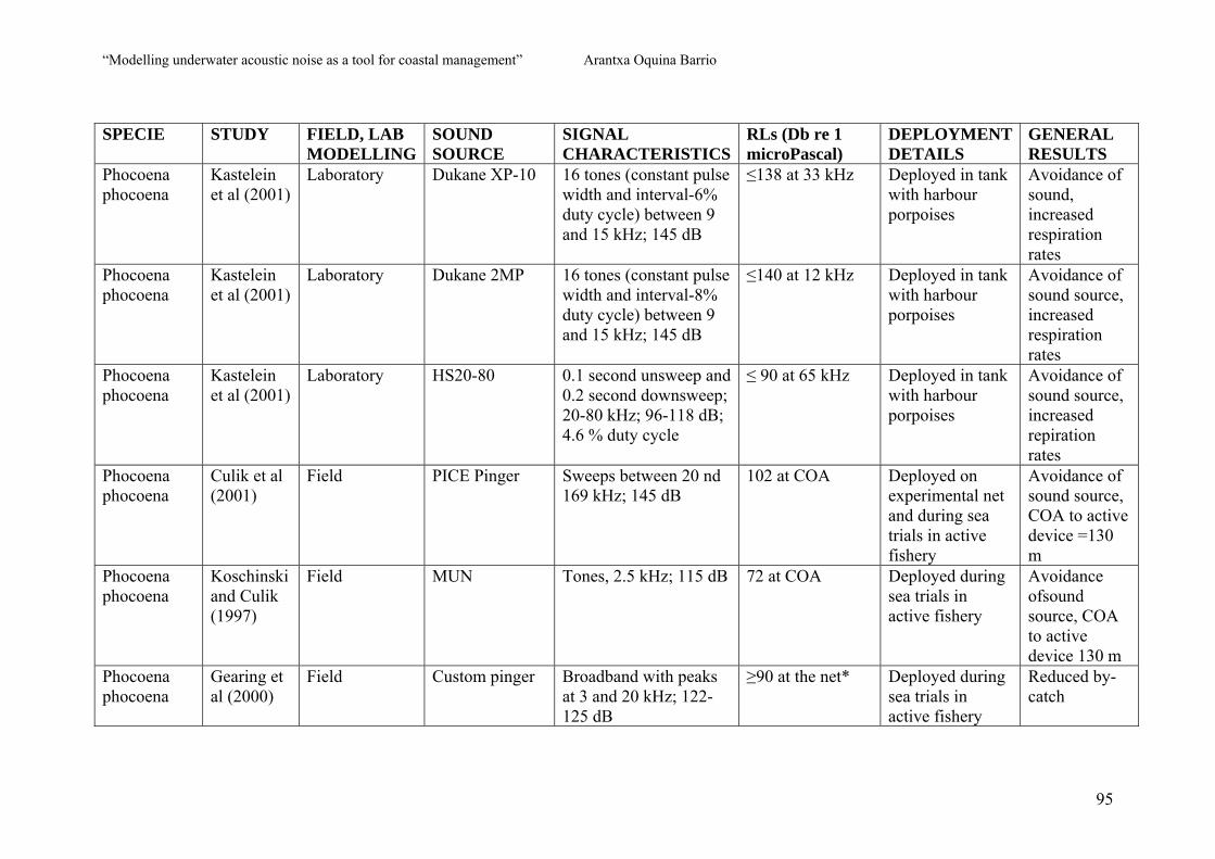
“Modelling underwater acoustic noise as a tool for coastal management” Arantxa Oquina Barrio
95
SPECIE STUDY FIELD, LAB MODELLING
SOUND SOURCE
SIGNAL CHARACTERISTICS
RLs (Db re 1 microPascal)
DEPLOYMENT DETAILS
GENERAL RESULTS
Phocoena phocoena
Kastelein et al (2001)
Laboratory Dukane XP-10 16 tones (constant pulse width and interval-6% duty cycle) between 9 and 15 kHz; 145 dB
≤138 at 33 kHz Deployed in tank with harbour porpoises
Avoidance of sound, increased respiration rates
Phocoena phocoena
Kastelein et al (2001)
Laboratory Dukane 2MP 16 tones (constant pulse width and interval-8% duty cycle) between 9 and 15 kHz; 145 dB
≤140 at 12 kHz Deployed in tank with harbour porpoises
Avoidance of sound source, increased respiration rates
Phocoena phocoena
Kastelein et al (2001)
Laboratory HS20-80 0.1 second unsweep and 0.2 second downsweep; 20-80 kHz; 96-118 dB; 4.6 % duty cycle
≤ 90 at 65 kHz Deployed in tank with harbour porpoises
Avoidance of sound source, increased repiration rates
Phocoena phocoena
Culik et al (2001)
Field PICE Pinger Sweeps between 20 nd 169 kHz; 145 dB
102 at COA Deployed on experimental net and during sea trials in active fishery
Avoidance of sound source, COA to active device =130 m
Phocoena phocoena
Koschinski and Culik (1997)
Field MUN Tones, 2.5 kHz; 115 dB 72 at COA Deployed during sea trials in active fishery
Avoidance ofsound source, COA to active device 130 m
Phocoena phocoena
Gearing et al (2000)
Field Custom pinger Broadband with peaks at 3 and 20 kHz; 122-125 dB
≥90 at the net* Deployed during sea trials in active fishery
Reduced by-catch

“Modelling underwater acoustic noise as a tool for coastal management” Arantxa Oquina Barrio
96
SPECIE STUDY FIELD, LAB MODELLING
SOUND SOURCE
SIGNAL CHARACTERISTICS
RLs (Db re 1 microPascal)
DEPLOYMENT DETAILS
GENERAL RESULTS
Phocoena phocoena
Trippel et al (1999)
Field Dukane netmark 1000
10 kHz pulses every 4 seconds; 132 dB
Detection range of 0.1-0.6 km for 80-90 dB RL
Deployed during sea trials in active fishery
Reduced by-catch
Phocoena phocoena
Carlstrom et al (2002)
Field Dukane netmark 1000
10 kHz pulses every 4 seconds; 132 dB
≥ 98 at the net Deployed during sea trials in active fishery
No by-catch recorded
Phocoena phocoena
Cox et al (2001)
Field Dukane netmark 1000
10 kHz pulses every 4 seconds; 132 dB
118-122 dB (ambient noise levels) at 125m
Deployed individually on mooring
Exclusion distance decreased by 50 % after 4 days
Phocoena phocoena
Johnston & Woodley (1998)
Field Various 180-200 dB 122 at max range of influence*
Assessed extent of AHD use on salmon farms in lower Bay of Fundy
Large percxentage of sites using AHDs. Possible habitat exclusion
Phocoena phocoena
Terhune et al (2002)
Field Airmar, Ferranti Thompson 4X special
195 and 166 dB respectively, 10-19 kHz
95 dB at 2.92 km for Airmar; 94 dB at 1.3 for Ferranti Thompson
AHDs deployed experimentally from small boat or on active salmon farms
Not Available
Phocoena phocoena
Jacobs & Terhune (2002)
Field Airmar 172 dB 158-164 dB at approximately 45 m
AHDs deployed on active salmon farms
Seals avoided sound source, COA= 45 m
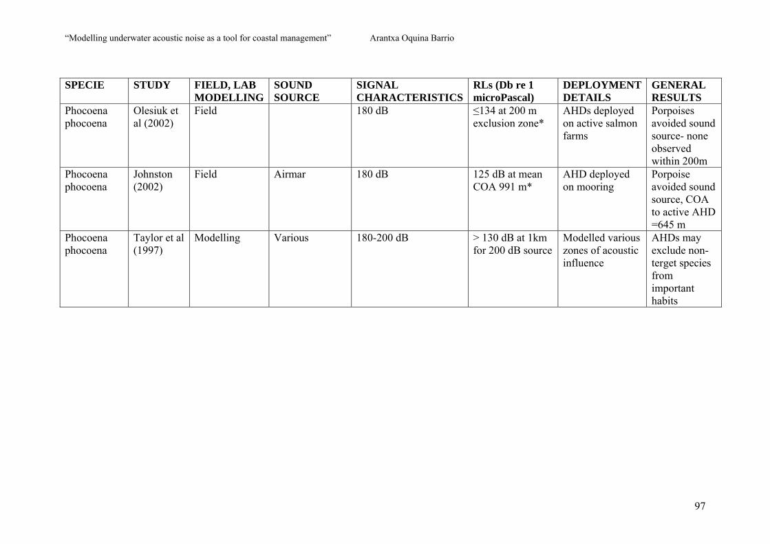
“Modelling underwater acoustic noise as a tool for coastal management” Arantxa Oquina Barrio
97
SPECIE STUDY FIELD, LAB MODELLING
SOUND SOURCE
SIGNAL CHARACTERISTICS
RLs (Db re 1 microPascal)
DEPLOYMENT DETAILS
GENERAL RESULTS
Phocoena phocoena
Olesiuk et al (2002)
Field 180 dB ≤134 at 200 m exclusion zone*
AHDs deployed on active salmon farms
Porpoises avoided sound source- none observed within 200m
Phocoena phocoena
Johnston (2002)
Field Airmar 180 dB 125 dB at mean COA 991 m*
AHD deployed on mooring
Porpoise avoided sound source, COA to active AHD =645 m
Phocoena phocoena
Taylor et al (1997)
Modelling Various 180-200 dB > 130 dB at 1km for 200 dB source
Modelled various zones of acoustic influence
AHDs may exclude non-terget species from important habits
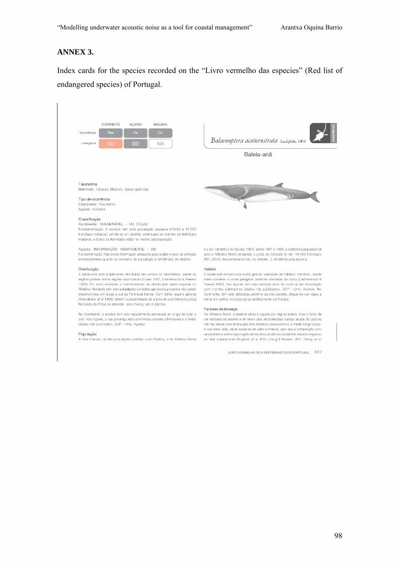
“Modelling underwater acoustic noise as a tool for coastal management” Arantxa Oquina Barrio
98
ANNEX 3. Index cards for the species recorded on the “Livro vermelho das especies” (Red list of
endangered species) of Portugal.
“Modelling underwater acoustic noise as a tool for coastal management” Arantxa Oquina Barrio
99
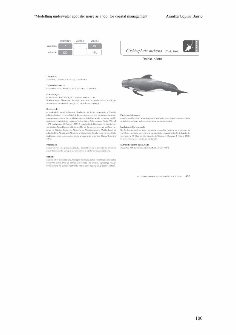
“Modelling underwater acoustic noise as a tool for coastal management” Arantxa Oquina Barrio
100

“Modelling underwater acoustic noise as a tool for coastal management” Arantxa Oquina Barrio
101

“Modelling underwater acoustic noise as a tool for coastal management” Arantxa Oquina Barrio
102
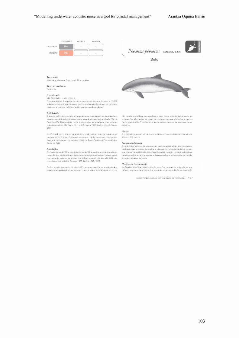
“Modelling underwater acoustic noise as a tool for coastal management” Arantxa Oquina Barrio
103
“Modelling underwater acoustic noise as a tool for coastal management” Arantxa Oquina Barrio
104

“Modelling underwater acoustic noise as a tool for coastal management” Arantxa Oquina Barrio
105

“Modelling underwater acoustic noise as a tool for coastal management” Arantxa Oquina Barrio
106
ANNEX 4. Tables with the conservation information in the “Livro vermelho das especies” of
Portugal, taken from the ICNB (Instituto da conservaçao da natureza
e a biodiversidade). http://portal.icnb.pt/ICNPortal/vPT2007/Homepage.htm
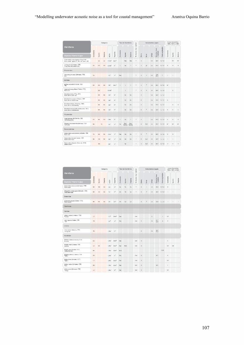
“Modelling underwater acoustic noise as a tool for coastal management” Arantxa Oquina Barrio
107


![12 Emergencias radiologicas ipen [Modo de Compatibilidade] Emergencias radiologicas ipen.pdf · O QUE É RADIAÇÃO ? • Propagação de energia de um ponto a outro do espaço ou](https://static.fdocuments.in/doc/165x107/5be375e709d3f2ad378bd341/12-emergencias-radiologicas-ipen-modo-de-compatibilidade-emergencias-radiologicas.jpg)