Modelling skewness and elongation in financial returns ...

Modelling skewness and elongation in financial returns th case of exchange-traded funds

Sanjiv Jaggia and Alison Kelly-Hawke

Recent studies have docmnented the importance of asymmetry and tailshyfatness of returns on portfolio-choice asset-pricing value-at-risk and option-valuation models This article explores the nature of skewness and elongation in dally Exchange-traded Fund (ETF) return distributions using g h and (~ x h) distributions These exploratory data analytic techniques of Tukey ( 1977) reveal patterns that are hidden from a cursory glance at conventional measures for skewness and elongation The g hand (g x h) distributions provide parameter estimates that indicate substantial variation in skevness and elongation fOr individual ETFs nonetheless some trends are discovered when the funds arc grouped by fund size and style of investing Monte Carlo simulations that these exploratory techniques arc able to capture patterns found in commonly used Generalized Autoregressive Conditional Heteroskedasticity (GARCH) family of models

I Introduction

This article explores the patterns of daily Exchangeshytraded Fund (ETF) return distributions ETFs are mutual funds that trade like stocks They are structured like index mutual funds that 1s a particular ETF contains a collection of stocks that typically track an index like the Dow Jones Industrial Average or the SampP 500 stock index An ETF thus com hines the valuation leature of a mutual fund with the tradability eature of a closed-end fund The advantage of examining the properties of ETFs over a particular index arises because ETFs tend to he more isolated frorn market microstructure noise such

as nonsynchronous trading as compared to an index In addition to analysing measures of return and risk for various ETFs a major goal o[ this article is to evaluate thoroughly the higher moments of skewness and kurtosis In particular this article explores the nature ofskewness and elongation in daily ETF return distributions using g hand (g x h) distributions

Numerous studies have documented that the form of the distribution of returns is a crucial assumption for meanmiddot variance portfolio theory theoretical models of capital asset prices and the prices ofcontingent claims 1

Statistical inference also relies heavily on distribushytional assumptions lf these assumptions are violated there are resulting implications for portfolio analysis

and Siddique (2000a) show how conditional skewness explains a significant part of the variation in returns even when factors based on size and book~toshymarket value arc added to the asset pricing modeL Dittmar (2002) incorporates skewness and kurtosis to the asset pricing model and his results indicate that nonlinearities substantially improve upon the models ability to describe a cross section of returns

Hansen (1994) introduces the generalized Students -distribution to model innovations of a Generalized Autoregressive Conditional Heteroskedasticity (GARCH) modeL This two parameter distribution is asymmetric and allows excess kurtosis which can also be used to model lime-varying conditional higher moments (Jondcau and Rockingcr 2003) Christoffersen et a (2006) develop a model of stock returns that allows for skewness as well as conditional heleroskedasticity and a leverage efecL They then introduce an option pricing formula consistent with this modeL Using SampP 500 stock options over the period 2January 1990 through 31 December 1992 inshysample and up to 10 weeks out-of-sample perforshymance of their model achieves a better fit than standard GARCH models

Ylost empirical studies calculate skewness and kurtosis as an average and find that stock market returns have negative skewness and severe excess kurtosis Given the presence of outliers however conventional measures of skewness and kurtosis may be quite inadequate in capturing the true behaviour of financial returns Kim and White (2004) show hmv a single outlier can dramatically influence convenshytional measures They conclude that one must look beyond conventional measures of skewness and kurtosis to gain insight into market returns behaviour

ln order to analyse ETF returns this article follows the exploratory data analytic techniques first suggested by Tukey (1977) and later applied lo a housing allowance demand experiment by Hoaglin (1985) These techniques are simple to compute and allow large flexibility and robustness in their fitting Badrinath and Chatterjee ( 1988) apply this technique to daily and monthly returns on the Center for Research in Security Prices (CRSP) equal-weighted and value-weighted market portfolios covering the period July 1962 through December 1985 They conclude that the distribution of the market portfolio is adequately explained as a skewed and elongated distribution ln subsequent work with daily commonshystock-return distributions Badrinath and Chatterjee (1991) find substantial variation in the parameter estimates for skewness and elongation for individual firms bul discover some trends across industry groups and firm sizes

Mills (1995) also uses exploratory dala techniques to examine the distribution of daily returns of three London Stock Exchange indices over the period 19R6 to 1992 He too concludes that returns are both skewed and extremely kurtotic However he rinds that the deregulation of the stock exchange in October 1986 and the run-up and aflermath of Black Monday (the market crash of 19 October 1987) alter the shape of the return distributions quite dramatically Dutta and Bahbel (2005) use the exploratory data analysis on 3-month London Interbank Oflcred Rate (LlBOR) data as implied by its option prices They find that the implied distribution is modelled more accurately by the g It and (g x h) distributions as compared to other commonly used distributions

The contributions of this article are threefold (l) to explore the nature of skewness and elongation in daily ETF return distributions using g h and (g x h) distributions proposed by Tukey (2) to search for patterns of skewness and elongation over different classes of ETFs (categorized by fund size and style of investing) that may enable investors to make more careful decisions in their portfolio selection and (3) to usc Monte Carlo simulations to analyse how well these exploratory techniques capture patterns found in commonly used GARCH family of models

Th(~ rest of th(~ article is orgmiz(~d as follows Section ll summarizes elements of lhe g It and (g x It) distributions and the estimation procedures Section HI provides descriptive statistics of the sample data and presents the results Section IV uses simulation based on GARCH models to analyse the sampling behaviour of the g h and (g x h) estimators Section V concludes and discusses implishycations for portfolio diversification models and portfolio selection

II The g h and (g x h) Distributions

Skewness and the g distribution

The skewness of a distribution is judged in tem1S or its departure from symmetry In tl1is application the random variable X is defined as the daily return on an ETF and Z is a standard normal random variable such that

( la)

where

(b)

The parameters A and B refer to the location and scale of X nspcctivcly 1l1c function Y(Z) is said to have the g-distribution where the parameter g controls the amount and direction of skewness thus a value of g= 0 corresponds to no skewness

ln order to estimate g we implement the approach suggested by Tukey (1977) that we let Xr x 1_r oP

and z-p represent the p-th and (1- p)th percentiles of the random variable X and a standard normal random variable Z respectively where p lt 05 Rewriting Equation Ia for the p-th and (1- p-th) percentiles gives

Xp=A+Bg[exp(gcp) I] (2a)

and

I] (2b)

Noting that Zp -= 1-p and x05 A+ Bj g[exp(gOJ- 1] A it follows from dividing Equation 2b from Equation 2a and solving lOr g yields

(3)

Thus gP measures skewness in terms of the logarithm of the relative distances of the (I p)th and the p-th percentiles Crom lhe medimL ivfuiLiple estimates or g may be obtained from Equation 3 by using selected values of p These estimates provide a srnnmary of hov skevv11ess changes across the sample and informative plots If the estimates of the gps are more or less constant then the median of these values can be used as an estimate of the overall skewness In addition the variation in these estimates provides information on the stability o[ the median estimate of g

In some cases the median may provide a good estimate of g but the power of this particular methodology stems from being able to focus on diferent percentiles of the distribution l11e typical approach to choosing the percentiles is to use letter values the sequence of percentiles is chosen such that p I2 corresponds to M (median) p = I4 correshysponds to F (fourths) p = 18 corresponds to E (eighths) and so on such that p= 116 132 164 1128 1256 etc are D B Z etc By definition the letter values pay more attention to the tails of the distribution than the middle since the tail area is repeatedly being halved

lf the data are symmetric the median is the point or syn1metry and each pair of letter values must be symmetrically placed about the median That the lowest fourth of the distribution will be as far below

the median as the upper fourth is from the median A simple way to check on symmetry is to define a set of mid summaries one for each of letter values The is the average of the two letter values (upper and lower) or I +-r-p] (The distance between the upper and lower values for any letter value [xp- is called the feller spread and the positive distance between the median and any letter value is called the lwllspread) In a perfectly symmetric distribution all midsummaries would be equal to the median l f the data were skewed to the right the midsummaries would increase as they came from the letter values further into the tails For data skewed to the left they would decrease lf apparent skevness is due to one or two stray values only the most extreme letter values and midsummaries would he affected

In order to analyse skewness graphically a plot of the sample upper values against the lower values should form a line with slope equal to -1 if the returns arc symmetric about the median A numerical estimate of the slope can be obtained by regressing sample upper values against sample lower values Testing would then reveal whether or not the slope is significantly different from l

Elongation and the h distribution

Elongation refers to the stretch of the tails of a distribution A more elongated distribution gives greater probability to outcomes that are quite notably more extreme Since there is no natural standard as symrnetry is for skewness a cornmon practice is to use the Gaussian distribution as the standard when measuring elongation ln this section we analyse elongation in the presence of symmetry The random variables X and Z are those previously defined such that

(4a)

where

(4b)

The function Yh(Z) is said to have the h distribution where the parameter I measures the elongation (or kurtosis) of _xmiddot If h=O there is no elongation relative to the Gaussian distribution for It gt 0 or h lt 0 the distribution exhibits thicker or thinner tails than the Gaussian distribution respectively

Analogous to the procedures used earlier an estimate of h is obtained by lirst rewriting Equation 4a for the pth and (1 p)th percentiles

or X noting that p= -Zt-pbull and subtracting XJ-p

from xP This process yields

(5)

The numerator on the left-hand side of Equation 5 is the letter spread while the denominator measures the corresponding distance (letter spread) for a unit normal random variable This value is defined as the pseudosigma or p~sigma and it measures the extent to which a distribution is more elongated than the Gaussian distribution That a value of p-sigma greater than one implies a distribution with thicker tails than the Gaussian distribution An estimate of I is obtained by ln( p-sigma) against for selected percentiles

Skewness elongation and the (g x h) distribution

Since skewness may induce elongation or both may exist in a distribution a joint assessment is necessary Here the (~ x h) distribution is obtained by multishyplying the g and h distributions Now the random variables X and Z are such that

(6a)

where

Jn order to estimate h conditionally on g or 1 we rework Equations 6a and 6b as done earlier to arrive at

h22)Bexp 11 (7)( 2

The left-hand side of Equation 7 is called the Corrected Full Spread (CFS) and an estimate of I can be obtained by regressing ln(CFS) on

Ill Descrlptlve Statlstlcs and Results

Data and descriptive statistics

The data for the sample are the time series of the daily adjusted closing price (adjusted for dividends and

splits) on an ETF that was continuously traded from l January 2003 to 31 December 2007 We calculate daily returns for each ETF as logarithmic price changes that is ln(p) -ln(p_)_ The source of the data is provided by http jfinanceyahoocom The total number of ETFs in the sample is 112 and for each ETF there are 1258 days of data For detailed analysis the sample is partitioned into six groups Funds arc first classified by fhnd size subgroups are (a) small funds 123) and (b) large funds (89) The size divisions rellect those used in the Morningstar investment style box Given fund funds are then classified by style of investing subgroups are (a) value (b) blend and (c) growth The appendix provides a detaileti explanation of how the funds are grouped middotwith respect to size and the style of investing

Table l reports summary statistics and convenshytional measures of skewness and excess kurtosir~ for the data set as a Vhole as well as each of the six subgroups The average daily return and SO for the entire data set arc 0062 and 1138 respectively The entire data set and all subgroups display skewness that is on average negative however the skewness coefficient over the entire sample ranges from -065 to 078 Not a single fund in the Small value or Small blend subgroup has a skewness coefficient In addition the average skewness coeffishycient for the Small value subgroup yields the most negative value while the corresponding statistic for the Large grotvth subgroup generates the least negative statistic~ interestingly these two subgroups have relatively low excess kurtosis

A return distribution vvith positive skewness has frequent small losses and a few extreme gains while a return distribution with negative skewness has frequent small gains and a few extreme losses Investors are likely to be attracted by positive skewness because the mean return ralls above the median (see Elton et a 2003 Reilly and Brown 2003 and the references therein) Relative to the rnean return positive skewness amounts to a limited though frequent dovnside compared with a somewhat unlimited but less frequent upside Harvey and Siddique (2000b) show that an investor may be Villing to accept negative expected return in the presence of large positive skewness

The entire sample and all subgroups are on average more elongated than the Gaussian distribution

Zmiddotwc have abo replicated this study using market adjmted rdurns computed agt ln(prfp~ ) -ln(mm ~ ) where m represnh1 1 1 the market (SampP 500) price at time t The results arc broadly similar to those using unadjusted returns These resultgt arc not indudOO in the article for the sake of brevity Excess kurtosis is deflned as kurtosis -3 ror the Gaussian distribution kurtosis equals 3 A posithe vaue of excess kurtosis implies a distribution that is simultaneously mere (l~ss) peaked and has fatter (thinner) tails than the Gaussian distribution

Table 1 Daily return characteristics of the sample of ETFs

Mean SD Skewness (min max) Excess k uriosis N

Entire sample (UJIJ2 L13S -lUR (-065 078) 2AO H2 Small value 0062 1072 -OAt (-057 -02) L74 9 Small blend 0058 0980 -026 (-030 -022) 055 6 Small growth (UJ61 L363 -OJ2 (-(U9026J 141 9 Large value 0064 1083 -022 (-065 021) 240 34 Lar)e hend 0067 Lll7 -06 (-055(t78) 391 19 Lar)e )rorth 0053 L219 -om (-042 o25J 169 15

NoCs All returns are In percent per Excess kurtosis= Kurtosis- 1

1ost nntahly the l~arge value anti the largP hlemf subgroups the subgroups containing the most ETFs have the highest average excess kurtosis coeIicients Such return distributions have a greater percentage of extremely large deviations from the mean return V1ost investors would perceive a greater chance of extremely large deviations from the mean as increasing risk In fact not a single ETF in the sample has negative excess kurtosis which would imply thinner tails than the Gaussian distribution However the Small blend subgroup has an average kurtosis coefficient of 055 Further analysis will reveal that some of the funds from this subgroup have elongation comparable to that of the Gaussian distribution

ssuming for a moment that the means and the SDs are not significantly different from one another for the various subgroups an investor may be inclined to avoid Small value and Small blend ETFs since all funds in these subgroups lack a positive skewness statistic Further an investor contemplating purchasing an ETF in the other four subgroups might focus solely on the fund vvithin each subgroup Vith the maximmn positive skewness and the smallest kurtosis statistic However these conventional meashysures of skewness and kurtosis do not reveal anything about the behaviour of skewness and kurtosis across the different tails of the distribution ~1oreover it is not possible to isolate any patterns from the data using only one measure A more thorough analysis of the data will reveal patterns that are hidden from a cursory glance at the conventional measures for skewness and kurtosis In many instances an investor equipped with this detailed information might make a radically different decision on which ETF to either purchase or avoid

Results from applying the g- and h-distribu6ons

For expositional purposes the ETFs with the mm1mum and maximum skewness coefficients from each subgroup arc selected for

Table 2 reports the Sharpe n1tio conventional rneasures of skewness and kurtosis as well as the g hand 1 statistics for each of these ETFs ln general funds with a negative (positive) conventional skewshyness coefficient yield negative (positive) median g values There are funds however for which the relative magnitude or the robust measure given by the rnedian g value is not consistent with its conventional skevness coefficient For instance BB2 Internet HOLDRs and Biotech HOLDRs have similar skewshyness coefficients with values of 026 and 025 respectively however the median g value of Biotech HOLDRs (0059) is more than three times that or BB2 Internet HOLDRs value t0019) Moreover BLDRS Developed Markets 100 ADR Index genshyerates the highest skewness coefficient in the entire sample yet its median g value of 0032 is by no means the highest value BLDRS Emerging Market 50 ADR has a slightly more negative skewness coefficient when compared to the value for ishares MSC Austria Index -042 versus -039 respectively but its median g value is more than three and a half times less negative than that for ishares MSCI Austria Index -0016 versus -0Jl58 respectively These results point to the fact that analysing the conventional measures for skevness and kurtosis may be 1nisleading

It is interesting to note that those ETFs with negative skewness tend to have the higher Sharpe ratios Even though the Sharpe ratio does not include skewness andor kurtosis explicitly studies have shovn that these higher moments are inherently priced For example Leland (1999) develops a model of market returns to show that investors seem to outperform the market if they are Villing to accept negatively skewed returns

Arguably it appears as if ETF managers are in some way selling risk in order to maintain good Sharpe ratios Similarly managers following a strategy of limiting downside risk are incorrectly underrated

Table 2 Higher moments of the sample of ETFs

Sharpe ratio Skewnc~s Kurtosis Median K h h

Small value Jshares CohenampStecrs Rty Majors lshares Russel 2000 Value lndex

(t04il 0()38

-057 -021

254 073

-(U02b -0048b

0053 0J)2J

(t049d 0022d

Small blend MidCap SPDRs Vanguard Exfd Mkt lnd VIPERs

0047 0055

~030

~022

042 046

-0075b -0037

0Jl05 0001

0003 0000

Small shares MSCI Austria Index BB2 Internet HOLDRs

0087 0009

-039 026

237 419

-0058b 0019

OoO NAG

-0037d NA

Large value StreetTRACKS DJ STOXX 50 Tdccomhldrs HOLDRs

0048 otm

-065 021

59 513

-0059b 0055b

OJOI OJ

fl099d 0116

LarKe hend hhare MSCI Australia Index BLDRS Asia 50 ADR Index

0072 0038

-055 078

210 3655

-0079b Of132b

0056 0289

0054 fl289d

Lar(C wowth BLDRS Emerging Market 50 ADR Biotech HOLD Rs

0059 0036

042 025

585 274

-0016h 0059

0119 0085

0119d 0056d

Notc The Sharpe ratio is calculated assuming a ri~k-free annual interest rate of 4dego

bWhen upper values arc regressed against lower values for the relevant suhgroup the slope igt significantly different from ~ at the 51Yo gtignificance level--- indicating that the distribution is not gtymmctric cVhen lnp-sigrna) is regressed against 2 the estimate of h (lhe slope) is signilkantly different from 0 al the 5~J1 signilkance levd indicating elongation thal deviates from the Gaussian distributior dWhen n(CFS) is regressed against ~2 lhe estimate of h (the slope) is different from 0 al the S1 significance levd indicating elongation that dcvJates from the GaussJan dislribui1on ern1e Vltllnes for hand z are nol 1vailahle (NA) for Jhi fnnd due Jn Jhe extraordinary nnmhcr cf0deg- return values Jn the sample

For a more detailed analysis of the g- and h-distributions we focus on the two funds within the Large blend subgroup Within this subgroup the ETF with the most negative skewness is the ishares IV1SCI Australia Fund (symbol EWA) with a skewness statistic of -055 while the ETF with the most positive skewness is the BLDRS Asia 50 ADR Index Fund (symbol ADRD) with a skewness statistic of 078 What is particularly striking about ADRD is the kurtosis coefficient of 3655 a value approximately 15 times the average kurtosis coefficient value in the entire sample Tables 3 and 4 present sample upper and lower letter values as well as midsummaries for 13 percentiles for these two ETFs

One should recall that for a symmetric distribution a plot of the upper values against the lower values would form a line with a slope equal to ~ 1 implying letter values that are equidistant from the median For EW A when the upper letter values are regressed against the lower values the slope has a value of -087 Further this value is statistically dilfcrent from the value of~ 1 at the 5 significance leveL The results indicate a rather substantial depumiddotture from synunctry a result reinforced once the g values

arc analysed For ADRD a regression of the upper values against the lower values reveals a slope of - Ll4 that also is statistically different from l at the 5deg0 level however positive skewness is implied here since 1- L141 is greater than 1- LOOI and an inspecshytion of the midsummaries (Table 4) indicates values that eventually mcrease as one moves further into the tails

ln order to further capture the behaviour of skewness in returns g values are estimated for different letter values to Equation 3 and are presented in Tables 3 and 4 In general a series that exhibits constant values for its estimates of g tends to have a simple pattern of skewness the lognormal distribution is such an example For EV A the median gvalue is -0079 and 12 of the 13g values are negative however there is considerable variation in the magnitude o[ the values An examination of ADRD reveals a median g value of 0032 however four of the 13 values are negative The patterns of skewness in these series are far from simple and suggests that they cannot be adequately explained by skewness coeficients of -055 for ADRD and 078 for EWA

Table 3 shareS VISCI Australia lude Fund I January 200~31 December 2007

Letter values for EVA

Lower Upper zr Midsummary g p-gtigma Corrected p~igma () (2) (3) (4) (5) (6) (7)

Oi62 0162 0 OJ62 0 -0538 0896 -0674 0179 0071 063 063

Ll86 408 -Ll50 0111 -0069 Ll27 ll26 -L790 LR54 -1534 ft032 -0093 88 85 -2594 2307 -1863 -(1144 -035 1316 1311 -3437 2678 -2154 -0380 -0166 1420 1413 -4039 3166 -2418 -(1437 -0139 1490 1481 -4379 3498 -2660 -0440 -0116 1481 1470 -4895 3825 -2886 -0535 -0112 1511 1498 -5443 4546 -3097 -0448 -0079 1613 1596 -)716 ltf) -197 -0 41 -0(14 1660 IMI -5858 5636 -34R7 -(ll11 -0017 1648 1627 -5930 5840 -3668 -0045 -0019 1604 15R2 -5965 5942 -3842 -0012 -0015 1550 1526

Note Columns L 2 4 6 and 7 are presented in terms of percentage returns StC text for definition of tcnns

Table 4 BLDRS Asia 50 A DR Index Fund~ 1 January 2003~31 Dlgtcember 2007

Le11er values for ADRD

Lower Upper z Mid summary g p-sigma Corrected (2) (3) (4) (5) (6) (7)

0 0 0 ()

-0409 0579 -0674 0085 0516 0733 (t7l2 -0945 1097 LIS 0 076 013 0888 0887 -1554 1611 1534 0029 0024 032 1031 -2278 2264 1863 -0 007 -0003 1219 1219 -3178 337 -1154 -0021 -OJJ06 1466 465 -4917 4~58 -2418 -0029 -0005 2022 2020 -8808 11532 -2660 1362 001 3823 389

12346 1266 -2886 -0090 -0005 4247 424 -14055 14422 -3097 0183 0008 4597 4590

14892 16529 -3297 0818 0032 4765 4756 -15219 17701 -3487 1241 0043 4720 471 -15383 18287 -366~ 1A52 0047 4589 4579 -15465 18580 - 3J~42 1558 0048 443 4420

Nme Columns 1 0 4 6 and 7 are pres~nted definition of hnm

ln order to determine whether the return series has thicker or thinner tails than the Gaussian distribushytion p-sigma estimates are calculated for different letter values using Equation 5 and are presented in Tables 3 and 4 A value of I implies neutral elongation or that of the Gaussian distribution An inspection of Table 3 reveals p-sigma estimates for EWA that appear greater than 1 suggesting fatter tails than the Gaussian According to Table 4 the p-sigma estimates for ADRD are even greater than those obtained for EVA An estimate of his obtained

in terms of percentage returns See text for

for each ETF by regressing ln(p-sigma) against z_ 12 for the selected letter values The h estimates for EWA and ADRD are 0056 and 0289 respectively Further testing reveals that the estimates of II for both funds are significantly diflcrcnt from 0 at the 5 significance leveL reflecting fatter tails than the Gaussian a common result with t1nancial return data

ln the above analysis of elongation an implicit assumption of symmetry was maintained Since skewness may induce elongation a joint assessment

is necessary Lsing median g estimates and Equation 7 corrected p-sigma estimates are calcushy

lated and are presented in Tables 3 and 4 Finally estimates of h are obtained by regressing ln(CFS) on

for the selected letter values The h estimates for EWA and ADRD arc 0054 and 0289 respectively where both estimates are statistically significant at the 5deg0 leveL

Within the Large blend subgroup judging EWA based on its conventional skevness statistic of -055 and kurtosis statistic of 210 would appear to be misguided Exploratory data techniques for this fund reveal a small negative median g estimate as well as an h estimate that is significantly different from 0 Fnrther_ since EWA s g estimates are quite variable across percentiles even the rncdian estimate is not representative orits overall skewness Similar findings are found once the other subgroups are analysed For example within the Small blend subgroup the Vanguard extended market index VIPER fund has one of the higher Sharpe ratios but a negative skewness coefficient of -022 and a kurtosis coeffishycient of OA6 Further this fund ha_gt a median g estimate of -0037 and hand h estimates of 0001 and 0000 respectively When upper values are regressed against lower values the slope is not statistically different from l indicating a distribution that is more or less sy1nmetric In addition the estimates of h and h are not signilicantly different from 0 reflecting elongation comparable to the Gaussian distribution An investor who avoids this fund on the basis of its relatively large negative skewness coefficient and kurtosis coericient of 046 might be making a poor decision

IV Simulation Based on GARCH Models

The GARCH models are used in modelling financial time series that exhibit time-varying volatility clustershying for example periods of swings followed by periods of relative calm These models have further been extended to include time-varying conditional higher moments As mentioned earlier the explanashytory data analysis of Tukey is attractive for its computational ease It is also considered robust to complex patterns of skewness and kurtosis in distributions In this section Ve study how well this exploratory captures the pat terns found in commonly used GARCH ltmily of models where the higher moments may or may not vary over time In particular we simulate data based on such models to analyse the sampling behaviour of the g II and h estimators

Consider continuously compounded returns r 1 = 100 ln (PfP1_ 1 ) for t = 1 2 T where rr=tltr+E The GARCH(l I) models the residual of a times series regression as f-1 = cr1t where zr is iid with E(c)=O Var(o)= I and conditional volamiddot tility is specilied as a= ao + bor7 1 + coo- 1bull We use 1000 observations to simulate the GARCH models in fact 1050 observations are considered but the first 50 observations are discarded to remove any influshyence from initial values The choie of parameters is consistent with the a vailahle evidence on market returns In pmmiddotticuhumiddot we use I 001900 =0956 along with a0 = 006 b0 = 005 and c0 = 090 for the analysis

The above parameter values mmiddotc used to si1nulatc the GARCH models where the residuals are drawn from the Gaussian Students t- and generalized Students shydistributions Although the Students -distribution allows for variations in the tail thickness it is considered restrictive since it is not consistent with a stylized fact that stock market returns are skewed The generalized Students -distribution offers flexshyibility in that it not only allows excess kurtosis (as in the standard Students -distribution) but also skewshyness (Hansen 1994) The two parameter density function of this distribution that is normalized to have zero mean and unit variance is

(8)

where 2 lt rJ lt oo and 1 lt ) lt 1 The constants are given by

a 2 I+41cG - r((~+ IJ2)

c (9)

This generalized distribution allows positive 0- gt 0) as well as negative ( lt 0) skewness Further it specializes to the Students middotdistribution when _ = 0 and to the Gaussian distribution for ) = 0 ~--+ oo For simulations we use the degrees of freedom parameter TJ = 6 to allow for excess kurtosis For departure from symmetry we use ) = -025 for negative skewness and) 025 for positive skewness

Kim and White (2004) use Monte Carlo simulashytions to demonstrate that the conventional measures of skewness and kurtosis arc very sensitive to outliers since they are based on the sample rncan which is known to he an i11adcquatc measure

Table 5 Simulation analysis of the g hand (g x It) distributions GARCH models with constant higher moments simulated tith the GatLlt~sian and Students t-distributionlt~

Gamsian Studenrs 1 (df=l=6)

Stati~tic g It It g h h

Median (Mean) 0000 (OJJOO) -OXH9 (-0119) -(UJ20 ( -(UJ 19) OJIOO (0000) (L05il (OJJ6l) 0057 (lUl60) Po s (199 s) -tW75 (IUJ78) -OJJ51 (0020) -(UJ51 ((Ul19) -0122 (OJ 32) -(tOOl (062) -OJ)() (ltl6l) P2 s (P9 s) -0 057 (0059) -0043 (0 ()]()) -0043 (00 10) -OJJ93 (0093) ()Oil (0 129) 0010 (0128) P (Psl -0 048 ((W49) -0040 (0 005) -(W40 (0005) -0078 (0077) ()017 (0114) 0017 (OJ 14) P25 (P75) -0 019 (00 19) -0028 (-0010) -0028 (-(W 10) -0032 (0032) ()()40 (0078) 0039 (0077)

Notes Rcsuli arc based on 5000 replications using a random smnple of 1000 observations drawn from the various distributions An aHowance is made for outliers Pr denotes the x-th percenttle value of the bootstrap distributions of g J and J

Table 6 Simulation analysis of the g It and (g x h) distributions GARCH models with constant higher moments simulated with the generalized Students t-distribution

1=6 )= -025 1]=6 )=025

Statistics g h h I( h h

Median (Mean) -OJ67 (-(U67) 0()56 (ft060) (t047 (0JJ50) OJ67 (OJ67) 0056 (ft060) (t047 ((UJ50) Po s (P9) -0290 (-0041) -OJXI2 (fU66) -fWIO (OJ 52) 0037 (0293) -0Jl03 (fU 75) -omo (ltU59J P2 s (P97 s) -0258 (-0069) OJXl9 (fU 31) fWOI (OJ 18) 0069 (0260) 0011 (fU31) ft002 (OJ 17) Ps(Pgs) -0244 (-0085) 0016 (0116) 0007 (OJ03l 0086 (0245) om7 (OJ6J 0008 (OJ03l Ps(Ps) -OJ 99 (-0136) 0038 (() 078) 0029 (()()67) OJ35 (0 199) 0038 (0078) 0029 (0067)

Note_ Results are based on 5000 replkations using a random sample of 1000 observations drawn from the variom distributions in allowance is made for outliers P denotes the x-th percentile value of the bootgttrap distributions of ff h and h

m such instances Although they do not consider Jhe g h and h statistics in heir analysis they do offer some other robust measures from the statistics lilerature We follow heir approach and use a mixture distribution that allows for outliers In particular if r~ is generated from D(tca) with probability p and from D(z vo) with probability l p then the random numbers used for simulations are generated by (p)D(a) (I -p)D(2a2) In the presence of outliers (p lt 1) we need to determine the relationship of (tza2) with (It a Following Kim and White we use the daily SampP index returns to approximate p 09988 lz p- 7 and a2 lOa

We use 5000 replications in our Monte Carlo analysis The hoolslrapping technique is used to analyse the sampling properties of the g h and h eslimators since their theorelical dislribution is not known These simulations shed light on the ability of the g h and h statistics to capture excess kurtosis and skewness when the data are generated by a GARCH process with outliers ln particular we usc the percentile method which for a given significance level a simply uses the and (I a2) percentiles of the bootstrap distribution to define the (1 a) 1(()~ coniidcncc interval for

a given parameter The confidence interval is then used to conduct a two-sided test for 11middot hand h For Instance the null hypothesis 0 is rejected at a given a if the percenlile inlerval [Pu12bull P1_1] for g does not include the hypothesized value of zero

ln Tables 5 and 6 we report some descriptive stalistics for g hand h in he GARCH models using the above-mentioned distributions for innovations When the distribution is Gaussian the sample mean and the sample median of g are both zero Implying that there is no evidence of skewness in the data Further since the 95(1 confidence interval for g using P25 and P97_5 is given by 0057 0059] we cannot reject the claim that the dala are symmetric ll=0) a a =(Ul5 For the Studens 1-distrihution wih six degrees of freedom the symmetry is correctly caplured a all significance levels However there is statistically significant evidence of excess kurtosis at the 10 and 5 levels For example at a 005 the entire ranges for hand h given by [001 lOJ29] and [0010 Ol2R] respectively are positive thus rejecting the null hypotheses fl0 h = 0 as well as fl0 h = ()

Results based on the generalized Students t-distribution for the residuals are presented in Table 6 We continue to usc six degrees of freedom

Table 7 Simulation analysis of the g hand (g x h) distributions GARCH models with time varying higher moments simulated tith the generalized Students t-4istribution

1] 0 6 -025 ij 6 f 025

Stati~tic g h h g h h

Median (Mean) -(U73 ( -(U 72) ()061 (0065) 0051 (0055) ()Jill (0160) 0060 ((064) 0051 (fl055) Po s (199 s) -0320 (-0020) 0001 (0176) -0007 (0161) 0007 (0293) 0()()2 (0172) -O()()R (fll64) P2 s (P9 s) -0281 (-0059) 0012 (0147) 0003 (0130) 0()48 (0263) ()()II (0140) 0003 (0129) P (Psl -0262 (-0078) 0019 (0127) 0 010 (0114) 0065 (0246) 0017 (0124) 0009 (0113) P25 (P75) -0209 (-0136) Oo42 (0084) 0032 (0072) OJ24 (0196) 0041 (00amp3) 0032 (0073)

Notes Results are baed on 5000 replicaiions using a random sample of WOO observations drawn from the various distributions An allowance is made for outliers Pr denotes the x-th percentile vaue of the bootstrap distributions ofg hand h

denoted by ~ = 6 One should recall that the skewness parameter falls in the interval -1 lt r lt l When we usc A= the 951 confidence interval for g is

0258 0069] This range is entirely negative suggesting statistically significant skewness Similarly for middot = 025 the range [0069 0260] indicates positive skewness or course the power of the tests will decrease (increase) as ])] approaches zero (one)

Although the hypotheses for hand h are difficult to interpret for skewed distributions they are broadly suggestive of excess kurtosis For instance for A= -025 the confidence intervals for h and h given by [00090131] end [OOOUU l respectively are entirely positive We would also like to point out that for ell distributions the sample mean of g equals its sample median whereas for h and h the mean is consistently e little higher than the median This result may be useful in developing the asymptotic distributions lOr these estimators

In order to include time-varying higher moments we treat the parameters of the generalized Students -distribution as functions o[ the conditioning inforshymation (Hansen 1994 Jondeau and Rockinger 2003) Consider =a+ brt--middot1 + ctit--middot1 and pound1 = a1 + b2ct--1 + where the transformations

moments and compare it with the Table 6 results that are based on constant higher moments It is noteworthy that the time-varying fJr and J paramshyeters introduce some extra noise in the data which makes the skewness and kurtosis estimators less precise However the results in Tables 6 and 7 are qualitatively similar For instance when A= -025 the 95dego confidence interval for g based on timeshyvarying higher moments given by 0281 0059] is still entirely negative However this interval is slightly wider than the comparable 0258- 0069] range implied by higher moments that do not vary with time Similarly although the 95deg10 confidence intervals for h and h given by [00090131] and [0001 0118] respectively are slightly wider they still infer a statistically significant excess kurtosis in the data

ln summary Ve rind that the exploratory data analysis of Tukey is attractive not only for its computational ease but also for its flexibility and robustness to various GRCH specifications with outliers Monte Carlo simulations suggest that theg h and h estimators are able to capture the skewness and excess kurtosis found in commonly used GARCH family of models where the higher moments may or may not vary over time A preliminary explanatory analysis can actually be used as a tool for identifying

are used to ensure that 2 lt fJ lt oo and - 1 lt A lt L For simulations we use a1 -036 h1 012 c1 =080 for computing ~~ and a2 012 (or a2 -012) h2 020 c1 = 0775 for f Ve choose these paramshyeter values to keep the problem tractable and comparable to the analysis Vith constant higher moments The unconditional sample means of these parameters are~ 6 and f 025 (or~ -025)

ln Table 7 we use the exploratory analysis of the data that arc generated by time-varying higher

a relevant GARCH modeL Ve vould like to point out that these estimators are likely to be robust to more co11nplltox patterns than those implied by the GARCH models that we considered in our simulations

V Conclusion

The vest majority of ETF return distributions point to distributions that are highly non-Gaussian when conventional 1neasures of skewness and kurtosis arc calculated This evidence alone suggests the

inadequacy of the traditional two~paramcter ie mcan~variancc rnodcl of portfolio diversification tforeover conventional measures of skewness and kurtosis might give misleading information concernshying the true behaviour of financial returns These measures are known to be sensitive to outliers and do not reveal anything about the behaviour of skewness and kurtosis across the tails o[ the distribution

We found that investors should not rely on single measure of skewness and kurtosis to summarize ETF return distributions The g hand (g x h) distributions provide robust pararncter estimates that arc not always consistent with their conventional countershyparts 1oreover Ve find substantial variation in skewness and kurtosis for individual ETFs The robust estimators of higher moments help us discover some trends when the funds are grouped by fund size and style of investing We also find that ETFs with negative skewness tend to have higher Sharpe ratios This result seems to suggest that ETF managers arc perhaps selling risk in order to maintain good Sharpe ratios and managers following a limiting downside risk strategy are incorrectly underrated Finally tfonte Carlo simulations suggest that these exploratory techniques are able to capture patterns found in commonly used GA RCH family or models

Acknowledgements

This article has benefited immensely from insightful comments or an anonymous referee We also thank Carlos Morales for uselhl comments Any errors are ours alone

References Akgiray V and Booth G G (19RX)The siable-law model

of ~tock return~ Journal rl Business and Economic Statistic ti 51 7

Badrinath S G and Chatterjee S (1988) On measuring sk~wness and elongation tn common stock return

distributions the case of the market index Journal of Business 61 451---72

Badrinath S G and Chatterjee S (1991) datHmaiytic look at ~kewness and elongation Jn common stock return distributions Journal rl Busines and lconomic Statistics 9 223 33

Christoffersen P Heston S and Jacob~ K (2006) Option valuation with conditional sk~wness Journal ( Econometrics 131 253-middotmiddotmiddot114

Dittmar R (2002) Nonlinear pricing kernels kurtosis pref~renc~ and evidence from th~ cross s~cton of equity returns The Journal of Finance 57 369403

Dulla K K and Babbd D F (2005) Extracting probabHistk information from the prices of interest raie options Journal of Busines 78 R4l 70

Elton E Gruber fvL Brown S and Goetzmann W (2003) 1~fodem Port(olio Thcvry and lilVCmcnt AnaJvsis 6th edn Viley New York

Hansen B E (1994) Autoregressive conditional density esiimaiion lntemationa Economic Review 35 705 30

Harvey C and SiddJque A (2000a) Conditional skewne~s in as~et pricing tests The Journal of Finance 55 1263~95

Harvey C and Siddique A (2000b) TJme~varying condi~ tional skewness and the mark~t risk premium Research in Banking and Fimmce i 27~~60

D (1985) Using to Exploring Data Tables Trendgt and Shapes

D Hoaglin F Mosteller and J New York pp 417middot60

Jonde-au E and Rocking~r M (2003) Conditional volatility sk~wness and kurtosis existence persisshytence and comovement~ Journal rl Economics Dynamic and Control 27 1699---737

Kim T-I-L and middotwhJte H (2004) On more rohust estimation of skewness and kurto~i~ Finance Research Letters 1 56---73

Kon S (19X4) Models of stock returns --- a comparison Journal oFinance 39 149---65

Leland H (1999) Beyond mean-variance performance mea~urement in a nonsy1nmetrical world Financial Analysts Journal 55 27-middotmiddot-36

Mills T 0 995) Modelling skewne~s and kurtosis in the London stock exchange FT-SE index return distribushytions The StafLgticicm 44 323middotmiddotJ2

R~my F and Brown K (2003) bHcstmcnt Analysis ami Port(Jio tfanagenwnt 7th -xln South-Vestern Mason OH

Tukey J (1977) E-rploratory Data Analysis AddisonshyWesley Reading Mk

Appendix Morningstar Style Box

The Y1orningstar style box is a tool that represents the characteristics of a imd in a graphical format There are two pieces of data that determine where the fund falls within the style box The first piece of data is market capitalization that the size of a lind Large funds medium-sized funds and s1nall funds are placed in the top row the middle row and the bottom row respectively of the style box IIorningstar calculates the market capitalization ofeach stock in the fund and accounts for its weighting in the fund in order to arrive at a number that best represents how the fund is positioned in the style box

Fnrther Ta hie A 1 shows that the Tvforningstar style box incorporates the size of the fund relative to the region where the fund invests That an ETF that tracks the United States with a market capitalshyization of $300 (in millions of dollars) is categorized as a small fund whereas an ETF tracking Canada with the same market capitalization is categorized as a medium-sized fund

For the sample in this article l1orningstar defined 89 large ETFs 14 medium-sized ETFs and 9 small ETFs ln order to conduct a detailed analysis given the style of investing and ensure a large enough sample with respect to subgroups it was necessary to combine 1nedium-sized funds with s1nall-sized funds This sum 23 hnds is referred to as small funds in this article

Table Al l1arket capitalization breakpoints in millions of tlS dollars

Region Large Medium Small

UnJted States 922541 15il5J9 44914 Canada 389693 75435 16871 Latin Am~rica 376903 105855 29l29 Europe Japan

803751 379151

150140 75711

35377 21()01

AustraliaNew Zealand 361643 70361 125()() AJa ex-Japan 198189 29778 8720

The other factor that determines a imds placement in the style box is its investment style Morningstar uses a number or statistics for each stock in a fund (long-term projected earnings growth historical earnings growth sales growth priceprojected earnings price-tomiddotbook etc relative to other stocks ln its market-cap range) and calculates a growth score and a value score each score will range from 0 to 100 Morningstar arrives at a stocks investment style by subtracting its value score from its growth score A stock with a strongly negative score is assigned to value and one with a strongly positive score is assigned to growth Those in between are categorized as blend The funds overall style is based on the weighted average of the style scores for all of its stocks

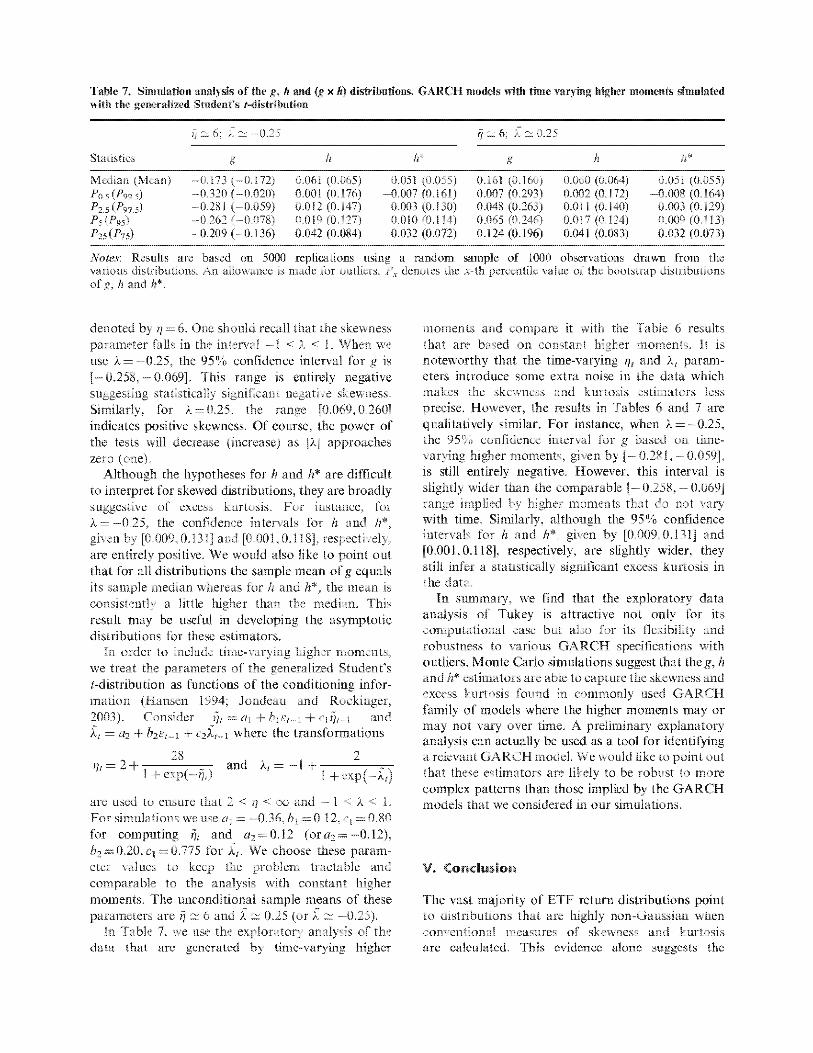and Siddique (2000a) show how conditional skewness explains a significant part of the variation in returns even when factors based on size and book~toshymarket value arc added to the asset pricing modeL Dittmar (2002) incorporates skewness and kurtosis to the asset pricing model and his results indicate that nonlinearities substantially improve upon the models ability to describe a cross section of returns

Hansen (1994) introduces the generalized Students -distribution to model innovations of a Generalized Autoregressive Conditional Heteroskedasticity (GARCH) modeL This two parameter distribution is asymmetric and allows excess kurtosis which can also be used to model lime-varying conditional higher moments (Jondcau and Rockingcr 2003) Christoffersen et a (2006) develop a model of stock returns that allows for skewness as well as conditional heleroskedasticity and a leverage efecL They then introduce an option pricing formula consistent with this modeL Using SampP 500 stock options over the period 2January 1990 through 31 December 1992 inshysample and up to 10 weeks out-of-sample perforshymance of their model achieves a better fit than standard GARCH models

Ylost empirical studies calculate skewness and kurtosis as an average and find that stock market returns have negative skewness and severe excess kurtosis Given the presence of outliers however conventional measures of skewness and kurtosis may be quite inadequate in capturing the true behaviour of financial returns Kim and White (2004) show hmv a single outlier can dramatically influence convenshytional measures They conclude that one must look beyond conventional measures of skewness and kurtosis to gain insight into market returns behaviour

ln order to analyse ETF returns this article follows the exploratory data analytic techniques first suggested by Tukey (1977) and later applied lo a housing allowance demand experiment by Hoaglin (1985) These techniques are simple to compute and allow large flexibility and robustness in their fitting Badrinath and Chatterjee ( 1988) apply this technique to daily and monthly returns on the Center for Research in Security Prices (CRSP) equal-weighted and value-weighted market portfolios covering the period July 1962 through December 1985 They conclude that the distribution of the market portfolio is adequately explained as a skewed and elongated distribution ln subsequent work with daily commonshystock-return distributions Badrinath and Chatterjee (1991) find substantial variation in the parameter estimates for skewness and elongation for individual firms bul discover some trends across industry groups and firm sizes

Mills (1995) also uses exploratory dala techniques to examine the distribution of daily returns of three London Stock Exchange indices over the period 19R6 to 1992 He too concludes that returns are both skewed and extremely kurtotic However he rinds that the deregulation of the stock exchange in October 1986 and the run-up and aflermath of Black Monday (the market crash of 19 October 1987) alter the shape of the return distributions quite dramatically Dutta and Bahbel (2005) use the exploratory data analysis on 3-month London Interbank Oflcred Rate (LlBOR) data as implied by its option prices They find that the implied distribution is modelled more accurately by the g It and (g x h) distributions as compared to other commonly used distributions

The contributions of this article are threefold (l) to explore the nature of skewness and elongation in daily ETF return distributions using g h and (g x h) distributions proposed by Tukey (2) to search for patterns of skewness and elongation over different classes of ETFs (categorized by fund size and style of investing) that may enable investors to make more careful decisions in their portfolio selection and (3) to usc Monte Carlo simulations to analyse how well these exploratory techniques capture patterns found in commonly used GARCH family of models

Th(~ rest of th(~ article is orgmiz(~d as follows Section ll summarizes elements of lhe g It and (g x It) distributions and the estimation procedures Section HI provides descriptive statistics of the sample data and presents the results Section IV uses simulation based on GARCH models to analyse the sampling behaviour of the g h and (g x h) estimators Section V concludes and discusses implishycations for portfolio diversification models and portfolio selection

II The g h and (g x h) Distributions

Skewness and the g distribution

The skewness of a distribution is judged in tem1S or its departure from symmetry In tl1is application the random variable X is defined as the daily return on an ETF and Z is a standard normal random variable such that

( la)

where

(b)





and

I] (2b)


(3)








(4a)

where

(4b)





(5)




(6a)

where


h22)Bexp 11 (7)( 2
























(t04il 0()38

-057 -021

254 073

-(U02b -0048b

0053 0J)2J

(t049d 0022d


0047 0055

~030

~022

042 046

-0075b -0037

0Jl05 0001

0003 0000


0087 0009

-039 026

237 419

-0058b 0019

OoO NAG

-0037d NA


0048 otm

-065 021

59 513

-0059b 0055b

OJOI OJ

fl099d 0116


0072 0038

-055 078

210 3655

-0079b Of132b

0056 0289

0054 fl289d


0059 0036

042 025

585 274

-0016h 0059

0119 0085

0119d 0056d










Oi62 0162 0 OJ62 0 -0538 0896 -0674 0179 0071 063 063






0 0 0 ()

-0409 0579 -0674 0085 0516 0733 (t7l2 -0945 1097 LIS 0 076 013 0888 0887 -1554 1611 1534 0029 0024 032 1031 -2278 2264 1863 -0 007 -0003 1219 1219 -3178 337 -1154 -0021 -OJJ06 1466 465 -4917 4~58 -2418 -0029 -0005 2022 2020 -8808 11532 -2660 1362 001 3823 389

12346 1266 -2886 -0090 -0005 4247 424 -14055 14422 -3097 0183 0008 4597 4590

14892 16529 -3297 0818 0032 4765 4756 -15219 17701 -3487 1241 0043 4720 471 -15383 18287 -366~ 1A52 0047 4589 4579 -15465 18580 - 3J~42 1558 0048 443 4420














(8)


a 2 I+41cG - r((~+ IJ2)

c (9)









1=6 )= -025 1]=6 )=025










1] 0 6 -025 ij 6 f 025













V Conclusion




Acknowledgements






























803751 379151

150140 75711

35377 21()01







and

I] (2b)


(3)








(4a)

where

(4b)





(5)




(6a)

where


h22)Bexp 11 (7)( 2
























(t04il 0()38

-057 -021

254 073

-(U02b -0048b

0053 0J)2J

(t049d 0022d


0047 0055

~030

~022

042 046

-0075b -0037

0Jl05 0001

0003 0000


0087 0009

-039 026

237 419

-0058b 0019

OoO NAG

-0037d NA


0048 otm

-065 021

59 513

-0059b 0055b

OJOI OJ

fl099d 0116


0072 0038

-055 078

210 3655

-0079b Of132b

0056 0289

0054 fl289d


0059 0036

042 025

585 274

-0016h 0059

0119 0085

0119d 0056d










Oi62 0162 0 OJ62 0 -0538 0896 -0674 0179 0071 063 063






0 0 0 ()

-0409 0579 -0674 0085 0516 0733 (t7l2 -0945 1097 LIS 0 076 013 0888 0887 -1554 1611 1534 0029 0024 032 1031 -2278 2264 1863 -0 007 -0003 1219 1219 -3178 337 -1154 -0021 -OJJ06 1466 465 -4917 4~58 -2418 -0029 -0005 2022 2020 -8808 11532 -2660 1362 001 3823 389

12346 1266 -2886 -0090 -0005 4247 424 -14055 14422 -3097 0183 0008 4597 4590

14892 16529 -3297 0818 0032 4765 4756 -15219 17701 -3487 1241 0043 4720 471 -15383 18287 -366~ 1A52 0047 4589 4579 -15465 18580 - 3J~42 1558 0048 443 4420














(8)


a 2 I+41cG - r((~+ IJ2)

c (9)









1=6 )= -025 1]=6 )=025










1] 0 6 -025 ij 6 f 025













V Conclusion




Acknowledgements






























803751 379151

150140 75711

35377 21()01





(5)




(6a)

where


h22)Bexp 11 (7)( 2
























(t04il 0()38

-057 -021

254 073

-(U02b -0048b

0053 0J)2J

(t049d 0022d


0047 0055

~030

~022

042 046

-0075b -0037

0Jl05 0001

0003 0000


0087 0009

-039 026

237 419

-0058b 0019

OoO NAG

-0037d NA


0048 otm

-065 021

59 513

-0059b 0055b

OJOI OJ

fl099d 0116


0072 0038

-055 078

210 3655

-0079b Of132b

0056 0289

0054 fl289d


0059 0036

042 025

585 274

-0016h 0059

0119 0085

0119d 0056d










Oi62 0162 0 OJ62 0 -0538 0896 -0674 0179 0071 063 063






0 0 0 ()

-0409 0579 -0674 0085 0516 0733 (t7l2 -0945 1097 LIS 0 076 013 0888 0887 -1554 1611 1534 0029 0024 032 1031 -2278 2264 1863 -0 007 -0003 1219 1219 -3178 337 -1154 -0021 -OJJ06 1466 465 -4917 4~58 -2418 -0029 -0005 2022 2020 -8808 11532 -2660 1362 001 3823 389

12346 1266 -2886 -0090 -0005 4247 424 -14055 14422 -3097 0183 0008 4597 4590

14892 16529 -3297 0818 0032 4765 4756 -15219 17701 -3487 1241 0043 4720 471 -15383 18287 -366~ 1A52 0047 4589 4579 -15465 18580 - 3J~42 1558 0048 443 4420














(8)


a 2 I+41cG - r((~+ IJ2)

c (9)









1=6 )= -025 1]=6 )=025










1] 0 6 -025 ij 6 f 025













V Conclusion




Acknowledgements






























803751 379151

150140 75711

35377 21()01

















(t04il 0()38

-057 -021

254 073

-(U02b -0048b

0053 0J)2J

(t049d 0022d


0047 0055

~030

~022

042 046

-0075b -0037

0Jl05 0001

0003 0000


0087 0009

-039 026

237 419

-0058b 0019

OoO NAG

-0037d NA


0048 otm

-065 021

59 513

-0059b 0055b

OJOI OJ

fl099d 0116


0072 0038

-055 078

210 3655

-0079b Of132b

0056 0289

0054 fl289d


0059 0036

042 025

585 274

-0016h 0059

0119 0085

0119d 0056d










Oi62 0162 0 OJ62 0 -0538 0896 -0674 0179 0071 063 063






0 0 0 ()

-0409 0579 -0674 0085 0516 0733 (t7l2 -0945 1097 LIS 0 076 013 0888 0887 -1554 1611 1534 0029 0024 032 1031 -2278 2264 1863 -0 007 -0003 1219 1219 -3178 337 -1154 -0021 -OJJ06 1466 465 -4917 4~58 -2418 -0029 -0005 2022 2020 -8808 11532 -2660 1362 001 3823 389

12346 1266 -2886 -0090 -0005 4247 424 -14055 14422 -3097 0183 0008 4597 4590

14892 16529 -3297 0818 0032 4765 4756 -15219 17701 -3487 1241 0043 4720 471 -15383 18287 -366~ 1A52 0047 4589 4579 -15465 18580 - 3J~42 1558 0048 443 4420














(8)


a 2 I+41cG - r((~+ IJ2)

c (9)









1=6 )= -025 1]=6 )=025










1] 0 6 -025 ij 6 f 025













V Conclusion




Acknowledgements






























803751 379151

150140 75711

35377 21()01






Oi62 0162 0 OJ62 0 -0538 0896 -0674 0179 0071 063 063






0 0 0 ()

-0409 0579 -0674 0085 0516 0733 (t7l2 -0945 1097 LIS 0 076 013 0888 0887 -1554 1611 1534 0029 0024 032 1031 -2278 2264 1863 -0 007 -0003 1219 1219 -3178 337 -1154 -0021 -OJJ06 1466 465 -4917 4~58 -2418 -0029 -0005 2022 2020 -8808 11532 -2660 1362 001 3823 389

12346 1266 -2886 -0090 -0005 4247 424 -14055 14422 -3097 0183 0008 4597 4590

14892 16529 -3297 0818 0032 4765 4756 -15219 17701 -3487 1241 0043 4720 471 -15383 18287 -366~ 1A52 0047 4589 4579 -15465 18580 - 3J~42 1558 0048 443 4420














(8)


a 2 I+41cG - r((~+ IJ2)

c (9)









1=6 )= -025 1]=6 )=025










1] 0 6 -025 ij 6 f 025













V Conclusion




Acknowledgements






























803751 379151

150140 75711

35377 21()01











(8)


a 2 I+41cG - r((~+ IJ2)

c (9)









1=6 )= -025 1]=6 )=025










1] 0 6 -025 ij 6 f 025













V Conclusion




Acknowledgements






























803751 379151

150140 75711

35377 21()01









1=6 )= -025 1]=6 )=025










1] 0 6 -025 ij 6 f 025













V Conclusion




Acknowledgements






























803751 379151

150140 75711

35377 21()01




1] 0 6 -025 ij 6 f 025













V Conclusion




Acknowledgements






























803751 379151

150140 75711

35377 21()01





Acknowledgements






























803751 379151

150140 75711

35377 21()01










803751 379151

150140 75711

35377 21()01



Modelling skewness and elongation in financial returns ...

Documents

Transcript of Modelling skewness and elongation in financial returns ...