Modelling Polymer Flooding in Reservoir Simulations

Edoardo Guarnerio

Delft University of Technology, The Netherlands

March 13, 2018

Outline

1 Introduction

2 Multi-Phase flow in Porous Media• Water flooding• Polymer Flooding

3 Velocity Enhancement Effect• Constant factor model• Saturation dependent model

4 Numerical Schemes

5 Results and Conclusion

2 / 26

Recovery Phases

• Primary recovery: extraction by natural mechanisms

• Secondary recovery: injection of water (waterflooding) to keep highpressure

• Tertiary recovery: any other technique to maximize recovery, basedon oil displacement

• Polymer flooding: polymer is added to water

3 / 26

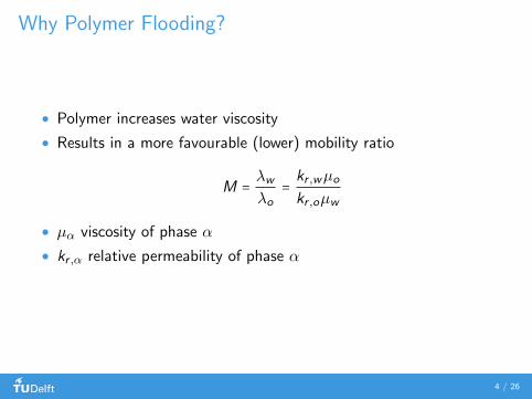
Why Polymer Flooding?

• Polymer increases water viscosity

• Results in a more favourable (lower) mobility ratio

M =λwλo

=kr ,wµo

kr ,oµw

• µα viscosity of phase α

• kr ,α relative permeability of phase α

4 / 26

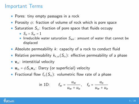
Important Terms

• Pores: tiny empty passages in a rock

• Porosity φ: fraction of volume of rock which is pore space

• Saturation Sα: fraction of pore space that fluids occupy• So + Sw = 1• Irreducible water saturation Swir : amount of water that cannot be

displaced

• Absolute permeability k: capacity of a rock to conduct fluid

• Relative permeability kr ,α(Sα): effective permeability of a phase

• vα: interstitial velocity

• uα = φSαvα: Darcy (or superficial) velocity

• Fractional flow fα(Sα): volumetric flow rate of a phase

in 1D: fw =uw

uw + uo, fo =

uouw + uo

5 / 26

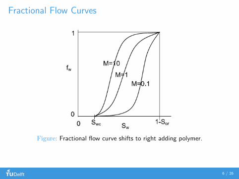
Fractional Flow Curves

Figure: Fractional flow curve shifts to right adding polymer.

6 / 26

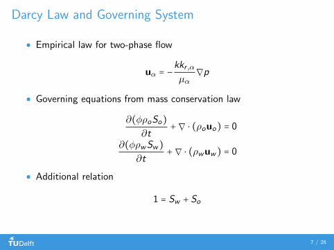
Darcy Law and Governing System

• Empirical law for two-phase flow

uα = −kkr ,α

µα∇p

• Governing equations from mass conservation law

∂(φρoSo)

∂t+∇ ⋅ (ρouo) = 0

∂(φρwSw)

∂t+∇ ⋅ (ρwuw) = 0

• Additional relation

1 = Sw + So

7 / 26

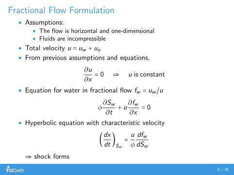
Fractional Flow Formulation• Assumptions:

• The flow is horizontal and one-dimensional• Fluids are incompressible

• Total velocity u = uw + uo• From previous assumptions and equations,

∂u

∂x= 0 ⇒ u is constant

• Equation for water in fractional flow fw = uw /u

φ∂Sw∂t

+ u∂fw∂x

= 0

• Hyperbolic equation with characteristic velocity

(dx

dt)Sw

=u

φ

dfwdSw

⇒ shock forms

8 / 26

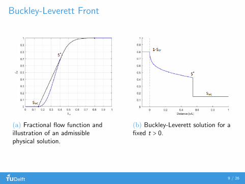
Buckley-Leverett Front

(a) Fractional flow function andillustration of an admissiblephysical solution.

(b) Buckley-Leverett solution for afixed t > 0.

9 / 26

Polymer Flood

• Extended fractional flow theory with further assumptions:• Polymer capillary forces and adsorption to rock are negligible• Polymer is present only in the aqueous phase

• Equations with polymer concentration c

φ∂Sw∂t

+ u∂(fw(Sw , c))

∂x= 0

φ∂(cSw)

∂t+ u

∂(cfw(Sw , c))

∂x= 0

• Two shocks arise

10 / 26

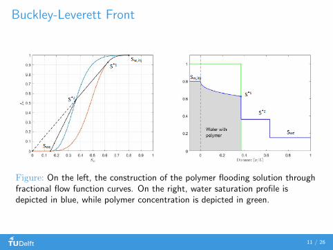
Buckley-Leverett Front

Figure: On the left, the construction of the polymer flooding solution throughfractional flow function curves. On the right, water saturation profile isdepicted in blue, while polymer concentration is depicted in green.

11 / 26

Inaccessible and Excluded Pore Volumes

• Inaccessible pore volumes (IPV): not all pores accessible topolymer

• Excluded pore volumes (EPV): layer close to the pore wall notaccessible to polymer

• Due to IPV and EPV polymer travels faster than an inert tracer

⇒ Velocity enhancement effect for polymer molecules

12 / 26

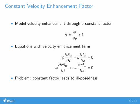
Constant Velocity Enhancement Factor

• Model velocity enhancement through a constant factor

α =φ

φp> 1

• Equations with velocity enhancement term

φ∂Sw∂t

+ u∂fw∂x

= 0

φ∂cSw∂t

+ αu∂cfw∂x

= 0

• Problem: constant factor leads to ill-posedness

13 / 26

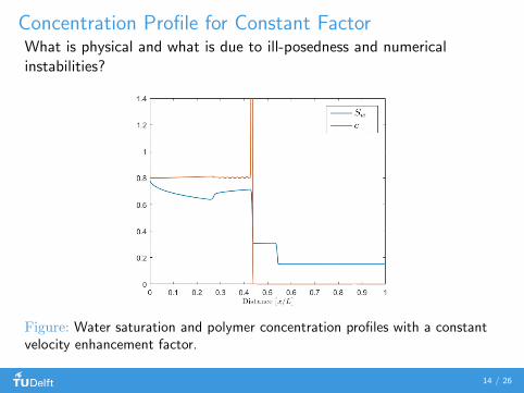
Concentration Profile for Constant FactorWhat is physical and what is due to ill-posedness and numericalinstabilities?

Figure: Water saturation and polymer concentration profiles with a constantvelocity enhancement factor.

14 / 26

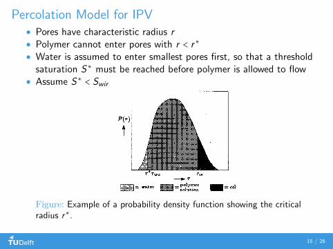
Percolation Model for IPV• Pores have characteristic radius r• Polymer cannot enter pores with r < r∗• Water is assumed to enter smallest pores first, so that a threshold

saturation S∗ must be reached before polymer is allowed to flow• Assume S∗ < Swir

Figure: Example of a probability density function showing the criticalradius r∗.

15 / 26

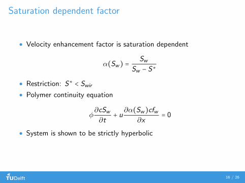
Saturation dependent factor

• Velocity enhancement factor is saturation dependent

α(Sw) =Sw

Sw − S∗

• Restriction: S∗ < Swir

• Polymer continuity equation

φ∂cSw∂t

+ u∂α(Sw)cfw

∂x= 0

• System is shown to be strictly hyperbolic

16 / 26

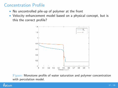
Concentration Profile• No uncontrolled pile-up of polymer at the front• Velocity enhancement model based on a physical concept, but is

this the correct profile?

Figure: Monotone profile of water saturation and polymer concentrationwith percolation model.

17 / 26

Model Extension

• Aim: derive a robust model to relax the restriction S∗ < Swir

• Tool: derive a necessary condition on α(Sw) for well-posedness

• Use theory from hyperbolic conservation laws

• Focus on IPV effect

18 / 26

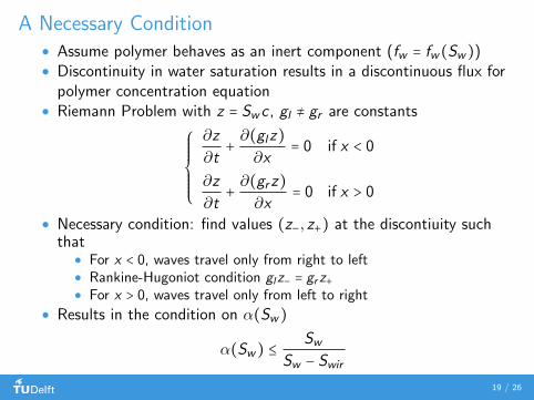
A Necessary Condition• Assume polymer behaves as an inert component (fw = fw(Sw))• Discontinuity in water saturation results in a discontinuous flux for

polymer concentration equation• Riemann Problem with z = Swc , gl ≠ gr are constants

⎧⎪⎪⎪⎪⎪⎨⎪⎪⎪⎪⎪⎩

∂z

∂t+∂(glz)

∂x= 0 if x < 0

∂z

∂t+∂(grz)

∂x= 0 if x > 0

• Necessary condition: find values (z−, z+) at the discontiuity suchthat

• For x < 0, waves travel only from right to left• Rankine-Hugoniot condition glz− = grz+• For x > 0, waves travel only from left to right

• Results in the condition on α(Sw)

α(Sw) ≤Sw

Sw − Swir

19 / 26

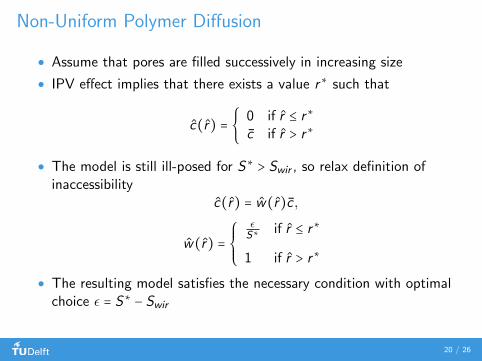
Non-Uniform Polymer Diffusion

• Assume that pores are filled successively in increasing size

• IPV effect implies that there exists a value r∗ such that

c(r) = {0 if r ≤ r∗

c if r > r∗

• The model is still ill-posed for S∗ > Swir , so relax definition ofinaccessibility

c(r) = w(r)c ,

w(r) =

⎧⎪⎪⎨⎪⎪⎩

εS∗ if r ≤ r∗

1 if r > r∗

• The resulting model satisfies the necessary condition with optimalchoice ε = S∗ − Swir

20 / 26

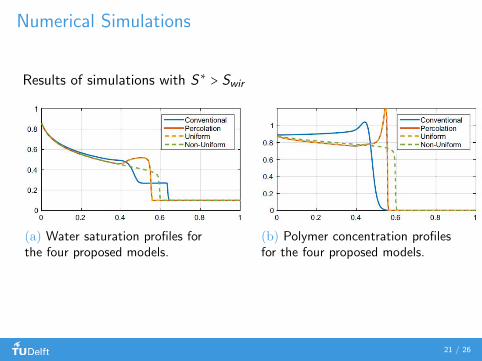
Numerical Simulations

Results of simulations with S∗ > Swir

(a) Water saturation profiles forthe four proposed models.

(b) Polymer concentration profilesfor the four proposed models.

21 / 26

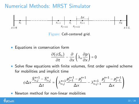
Numerical Methods: MRST Simulator

Figure: Cell-centered grid.

• Equations in conservation form

∂(φSα)

∂t−∂

∂x(λα

∂p

∂x) = 0

• Solve flow equations with finite volumes, first order upwind schemefor mobilities and implicit time

φ∆xSn+1α,j − Sn

α,j

∆t=⎛

⎝λn+1α,j

pn+1j+1 − pn+1j

∆x− λn+1α,j−1

pn+1j − pn+1j−1∆x

⎞

⎠

• Newton method for non-linear mobilities

22 / 26

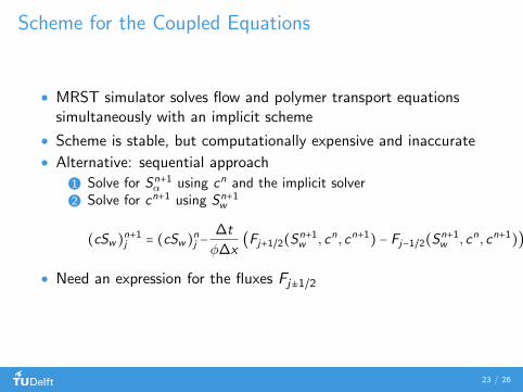
Scheme for the Coupled Equations

• MRST simulator solves flow and polymer transport equationssimultaneously with an implicit scheme

• Scheme is stable, but computationally expensive and inaccurate

• Alternative: sequential approach

1 Solve for Sn+1α using cn and the implicit solver

2 Solve for cn+1 using Sn+1w

(cSw)n+1j = (cSw)

nj −

∆t

φ∆x(Fj+1/2(S

n+1w , cn, cn+1) − Fj−1/2(S

n+1w , cn, cn+1))

• Need an expression for the fluxes Fj±1/2

23 / 26

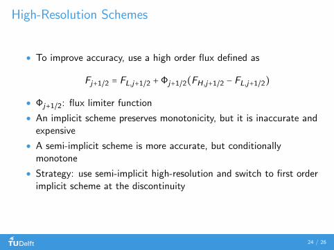
High-Resolution Schemes

• To improve accuracy, use a high order flux defined as

Fj+1/2 = FL,j+1/2 +Φj+1/2(FH,j+1/2 − FL,j+1/2)

• Φj+1/2: flux limiter function

• An implicit scheme preserves monotonicity, but it is inaccurate andexpensive

• A semi-implicit scheme is more accurate, but conditionallymonotone

• Strategy: use semi-implicit high-resolution and switch to first orderimplicit scheme at the discontinuity

24 / 26

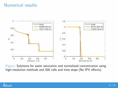
Numerical results

Figure: Solutions for water saturation and normalized concentration usinghigh-resolution methods and 500 cells and time steps (No IPV effects).

25 / 26

Conclusions

• Polymer flooding may considerably increase performance, but themodeling presents physical and numerical challenges

• A constant velocity enhancement factor leads to ill-posedness anduncontrolled sharp peaks

• Saturation dependent models result in a monotone profile, butthese models must be validated with physical experiments

• Common simulators still employ a constant factor

• Numerical schemes stability depends also on the adopted model ofvelocity enhancement

• Future work: acquire experimental data to validate appropriatemodels and derive robust numerical schemes

26 / 26