Modelling of spot welds for NVH simulations in view of...

Modelling of spot welds for NVH simulations in view of refined panel meshes Master’s Thesis in the Master’s programme in Sound and Vibration

TORSTEN EPPLER & ROLF SCHATZ Department of Civil and Environmental Engineering Division of Applied Acoustics Chalmers Vibroacoustics Group CHALMERS UNIVERSITY OF TECHNOLOGY Göteborg, Sweden 2007 Master’s Thesis 2007:150

MASTER’S THESIS 2007:150

Modelling of spot welds for NVHsimulations in view of refined panel meshes

TORSTEN EPPLER & ROLF SCHATZ

Department of Civil and Environmental EngineeringDivision of Applied Acoustics

Vibroacoustics GroupCHALMERS UNIVERSITY OF TECHNOLOGY

Goteborg, Sweden 2007

Modelling of spot welds for NVH simulations in view of refined panel meshes

© TORSTEN EPPLER & ROLF SCHATZ, 2007

Master’s Thesis 2007:150

Department of Civil and Environmental EngineeringDivision of Applied AcousticsVibroacoustics GroupChalmers University of TechnologySE-41296 GoteborgSweden

Tel. +46-(0)31 772 1000

Reproservice / Department of Civil and Environmental EngineeringGoteborg, Sweden 2007

Modelling of spot welds for NVH simulations in view of refined panel meshesMaster’s Thesis in the Master’s programme in Sound and Vibration

TORSTEN EPPLER & ROLF SCHATZDepartment of Civil and Environmental EngineeringDivision of Applied AcousticsVibroacoustics GroupChalmers University of Technology

Abstract

Today spot welding is the most common technique for connecting metal parts of anautomotive body. A few thousands of these spot welds are applied to a car bodyin-white during an automated assembly process. Therefore it’s obvious that the dy-namic behaviour of an automotive body is highly affected by these connections. Inthe Computer-Aided Engineering (CAE) processes exist different Finite Element (FE)modelling approaches for spot weld connections, depending on the area of interest likeNoise-Vibration-Harshness (NVH), durability etc. For NVH simulations ACM2 andCWELD spot weld approach are mostly used in industry.The aim of the present work is to investigate these most common spot weld models forNVH in view of a refined FE-mesh. In addition to the refined meshes the influence of adetailed thickness distribution over the metal sheets is studied. If necessary, an updat-ing process should be elaborated for the most suitable spot weld model, so that it canbe used with refined meshes. For validation purpose eigenfrequencies and frequencyresponse functions (FRF’s) from FE-simulation and measurements will be compared.

Keywords: Finite Element analysis, Structural dynamics, Spot weld, ACM2, CWELD,mesh refinement, NVH

iii CHALMERS, Master’s Thesis 2007:150

CHALMERS, Master’s Thesis 2007:150 iv

Contents

Abstract iii

Contents iv

Acknowledgements vii

1 Introduction 1

1.1 Aim of this thesis . . . . . . . . . . . . . . . . . . . . . . . . . . . . . . . . 21.2 Post processing Toolbox in Matlab . . . . . . . . . . . . . . . . . . . . . . . 2

2 Theoretical Background 5

2.1 CWELD . . . . . . . . . . . . . . . . . . . . . . . . . . . . . . . . . . . . . 52.2 ACM2 model . . . . . . . . . . . . . . . . . . . . . . . . . . . . . . . . . . 92.3 Literature review . . . . . . . . . . . . . . . . . . . . . . . . . . . . . . . . 13

3 The benchmark structures 17

4 Measurements 19

4.1 Pre-Investigations . . . . . . . . . . . . . . . . . . . . . . . . . . . . . . . . 194.2 Configuration . . . . . . . . . . . . . . . . . . . . . . . . . . . . . . . . . . 204.3 Eigenfrequencies & Damping . . . . . . . . . . . . . . . . . . . . . . . . . 214.4 Deviation for the sets of the three sidemember parts . . . . . . . . . . . . 22

5 Single sidemember panels 27

5.1 Mesh refinement . . . . . . . . . . . . . . . . . . . . . . . . . . . . . . . . 275.2 Mapped thickness distribution . . . . . . . . . . . . . . . . . . . . . . . . 335.3 Main results . . . . . . . . . . . . . . . . . . . . . . . . . . . . . . . . . . . 37

6 Investigations of welded assembly 39

6.1 ACM2 vs. CWELD . . . . . . . . . . . . . . . . . . . . . . . . . . . . . . . 406.2 ACM2 model . . . . . . . . . . . . . . . . . . . . . . . . . . . . . . . . . . 416.3 Reasons for stiffness loss with mesh refinement . . . . . . . . . . . . . . . 456.4 Influence of mapped thickness distribution . . . . . . . . . . . . . . . . . 466.5 ”RBE3 expansion” on ACM2 model . . . . . . . . . . . . . . . . . . . . . 48

v

6.6 ”RBE3 reconnection” on ACM2 model . . . . . . . . . . . . . . . . . . . . 52

7 Conclusion 55

References 57

A Single sidemember panels 59

CHALMERS, Master’s Thesis 2007:150 vi

Acknowledgements

First of all we want to thank the Department of Applied Acoustics for offering us thepossibility and providing us with all the needed support for conducting this thesiswork.Our special thank is dedicated to Professor Wolfgang Kropp and Andrzej Pietrzyk,which supervised our work and gave helpful advices in many discussions. But alsoall the other members of the department have to be mentioned, giving us help andhaving an open ear during the whole time.Also special thanks to Borje Wijk who spent a lot of time helping us all with the mea-surement equipment and especially in building up a workstation.Finally a big thank you to our Swedish landlord Kent Holzner and his whole family fordoing us our stay in Sweden as pleasantly as possible including the numerous unfor-getable sailing trips and dinners.

vii

CHALMERS, Master’s Thesis 2007:150 viii

1 Introduction

Spot weld modeling is the main joining technique for car body panels. For a typicalcar body one can assume several thousands of spot welds. The joining process itselfhappens with two electrodes applying pressure to the metal sheets when welding themtogether. The spot weld itself results from metal fusion. During that process the spotweld nugget gets a different material property like the original metal sheets and alsoa zone around the nugget is affected from the produced heat which affects as well thematerial properties.

For FEM simulation it is difficult to describe boundary conditions of those spot weldpositions precisely. From the point of view of NVH calculations it is obviously thatthese joints mainly influence the stiffness behavior of the whole structure. Thereforeseveral spot weld models have been created in the past. The most widely used spotweld models in industry are the CWELD model and the ACM2 model. The standardmodel at Volvo is the ACM2 model, because it has like the CWELD model the impor-tant benefit to be able to connect independently meshed structures together.

With increasing calculation power there is also a demand to refine the mesh size withthe aim to get more accurate simulation results at higher frequencies. The reason there-fore is, that components of a car body mainly consists of complex structures. Anotherimportant fact is, that the choice of finite element formulation is always a compromisebetween the demands of NVH-, Crash-, and Durability simulations. Also very smallholes and bolts can only be modeled exactly with small enough mesh sizes. On theother hand with further mesh refinement the position of spot welds and also their dy-namic properties should not be affected. Previous investigations at Volvo show that thecurrent modeling technique (ACM2) shows weakness with further refinement of thebody panel meshes.

1

1.1 Aim of this thesis

The aim of this thesis can be split up in following parts:

Preliminry part

1. Literature study regarding spot weld modeling in vehicle bodies.

2. Getting acquainted with MSC Nastran analysis procedures relevant for dynamicanalysis and development of a Postprocessing Toolbox in Matlab

Main part

1. Carrying out FRF tests on two sets of benchmark structures (inner and outerpanel) in free-free conditions

2. Carrying out simulations of the above experiments, including metal forming dataand different mesh densities

3. Carrying out FRF measurements on the welded benchmark structures

4. Carrying out simulations of the welded benchmark structure, using different spotweld models and mesh densities, including metal forming

5. Comparison of test results and simulation results

6. Selection of the most interesting candidates for future applications

1.2 Post processing Toolbox in Matlab

The FEM calculations in this thesis were done with MD Nastran. Nastran itself is onlythe solver which means that to carry out a whole analysis one has to work also withsome kind of Pre- and Postprocessor. The preprocessing process encircles the construc-tion of an FEM model with the help of available CAD data. The whole model was storedin a separate mesh-data-file. The analysis setup was stored in a separate analysis-file.The construction of all desired FEM models was done at Volvo. The calculation of themodels was done at Chalmers. To visualize the analysis results in some way it was nec-essary to load the numerical calculation results in Matlab. Therefore a postprocessingToolbox has been developed.

CHALMERS, Master’s Thesis 2007:150 2

The postprocessing Toolbox consists of following programmes:

• nas2mat.m : function which reads the whole mesh-file and stores it in a workspace.

• read eigenvector.m : function which reads the eigenvectors of all nodes from thePunch-file for each corresponding eigenfrequency and stores the eigenvectors ina workspace

• read FRF.m : function which reads the calculated displacement data from thePunch-files.

• calculate f r f .m : function which calculates all FRFs from the displacement results

• plot geometry.m : function which plots the whole mesh-data

• animate mode.m : function which animates the calculated modes of the structure

• plot mode.m : function which plots pictures from the mode shapes

3 CHALMERS, Master’s Thesis 2007:150

2 Theoretical Background

In this chapter a short overview will be given about spot weld models which are presentin literature. The focus is set on models which are normally used in the area of Noise-Vibration-Harshness (NVH) simulations.

2.1 CWELD

The CWELD approach was introduced in MSC.Nastran 2001 [09, 19]. Further elementdescriptions and verification investigations can be found in [02, 04]. The CWELD ele-ment full fills the main requirements that it can connect non congruent meshes as wellas congruent and the weld area is considered.With the CWELD element three types of connections can be defined:

• A Point to Point connection, where an upper and lower shell grid are connected

• A Point to Patch connection; where a grid point of a shell is connected to a surfacepatch

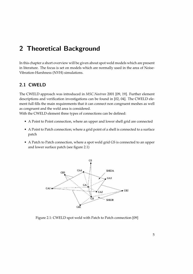
• A Patch to Patch connection, where a spot weld grid GS is connected to an upperand lower surface patch (see figure 2.1)

Figure 2.1: CWELD spot weld with Patch to Patch connection [09]

5

The Patch to Patch connection is the most general connectivity and is considered herein the following explanations. The center of the weld is defined by the spot weld gridGS, which is usually not a node in the FE-mesh and it isn’t required that GS lies onthe FE-geometry. The CWELD algorithm projects GS normal to the upper shell and theresulting piercing point is called GA. The direction GS-GA defines the piercing pointGB on the lower shell. The projected grids GA and GB define the length and directionof the spot weld itself.CWELD allows connections up to 10 layers and works with different element types.For example quadrilateral and triangular elements can be connected. A surface patchmust have at least 3 grids and has an upper limit of 8 grids.The spot weld itself is a short beam between GA and GB with 2x6 degrees of freedom(see figure 2.2). The element is a special shear flexible beam of the type Timoshenko.The Young’s modulus and spot weld diameter D are taken from the material definedon the PWELD property entry. The cross sectional properties like the shear modulusare calculated with the spot diameter D. The length of the beam is the distance betweenGA and GB.

Figure 2.2: Spot weld element [19]

If on the PWELD property SPOT is defined, an effective element length Le is defined,regardless of the true length like:

Le =12

· (ta + tB) (2.1)


ta and tB are the thickness of the involved plates (shells)

Then the Young’s and shear modulus E and G are scaled by the ratio of true lengthto the effective length:

!E = E · LLe

!G = G · LLe

(2.2)

This scaling leads to a spot weld stiffness which is approximately constant for allelements. Additionally extremely elements with short lengths L and extremely softelements with long lengths L are avoided. If SPOT is not defined the true length is usedif it is inside the range:

LDMIN ! L/D ! LDMAX (2.3)

LDMIN and LDMAX could be defined by the user and are by default: LDMIN = 0.2and LDMAX = 5.0For the patch to patch connection the beam end points GA and GB are connected tothe shell grids of shell A and B with the help of constraint equations. The under-lying method is subsequently described and the equations are shown exemplary forgrid point A. The three translational DOF of grid GA are connected with the threetranslational DOF of the shell grid points using the interpolation functions of the corre-sponding shell surface. The three rotational DOF at grid GA are connected to the threetranslational DOF of the shell grid points with Kirchhoff conditions.

"#$

#%

uvw

&#'

#(A

= ! NI (!A, "A) ·

"#$

#%

uvw

&#'

#(I

(2.4)

#Ax =

$w$y

= ! NI,y · wI

#Ay = "$w

$x= "! NI,x · wI

#Az =

12

)$v$x

" $u$y

*=

12

+! NI,x · vI "! NI,y · uI

,

(2.5)

NI : shape functions of the surface patch!A and "A : normalized coordiantes of GAu, v, w : displacements#x, #y, #z : rotations


These 6 equations are written in the local tangent system of the surface patch at pointGA. The normal direction is z and the tangent directions are x and y. The patch to patchconnection ends up with 12 constraint equations.For the formats GRIDID and ELEMID, the grid points are corresponding with gridpoints of shell elements. For the new formats ELPAT and PARTPAT, the grid points areauxiliary points GAHI and GBHI, I=1,4, constructed like shown in figure (2.3).

Figure 2.3: Cross sectional area and auxiliary points GAHI and GBHI for formats EL-PAT and PARTPAT [19]

The auxiliary points are connected to shell element grids with a second set of follow-ing constraints:

"#$

#%

uvw

&#'

#(I

= !K

GIK ·

"#$

#%

uvw

&#'

#(K

(2.6)

GIK : coefficient matrix derived from RBE3 type constraintsK : shell grid points

With the formats ELPAT and PARTPAT, the CWELD element can connect from one upto 3x3 elements on shell A resp B, which is presented in figure (2.4)


Figure 2.4: Connectivity for formats ELPAT and PARTPAT [19]

Studies in [2] show that the CWELD approach simulates the force transfer between apatch to patch connection accurately for

D/S ! 1.0 (2.7)

D : spot diameterS : mesh size (length of shell element)

2.2 ACM2 model

In [03] the ACM2 model was proposed. Figure (2.5) shows a typical construction ofthe model. The ACM2 model consists of a brick element which is coupled at the cor-ners to the upper and the lower shell elements over RBE3 elements. All connectedshell elements build up a so-called patch area. The RBE3 elements are interpolation el-ements which make it possible to connect two non-congruent meshes without the needto remesh around the coupling zones.


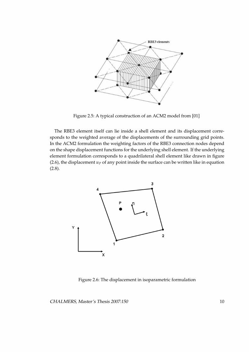
Figure 2.5: A typical construction of an ACM2 model from [01]

The RBE3 element itself can lie inside a shell element and its displacement corre-sponds to the weighted average of the displacements of the surrounding grid points.In the ACM2 formulation the weighting factors of the RBE3 connection nodes dependon the shape displacement functions for the underlying shell element. If the underlyingelement formulation corresponds to a quadrilateral shell element like drawn in figure(2.6), the displacement uP of any point inside the surface can be written like in equation(2.8).

Figure 2.6: The displacement in isoparametric formulation


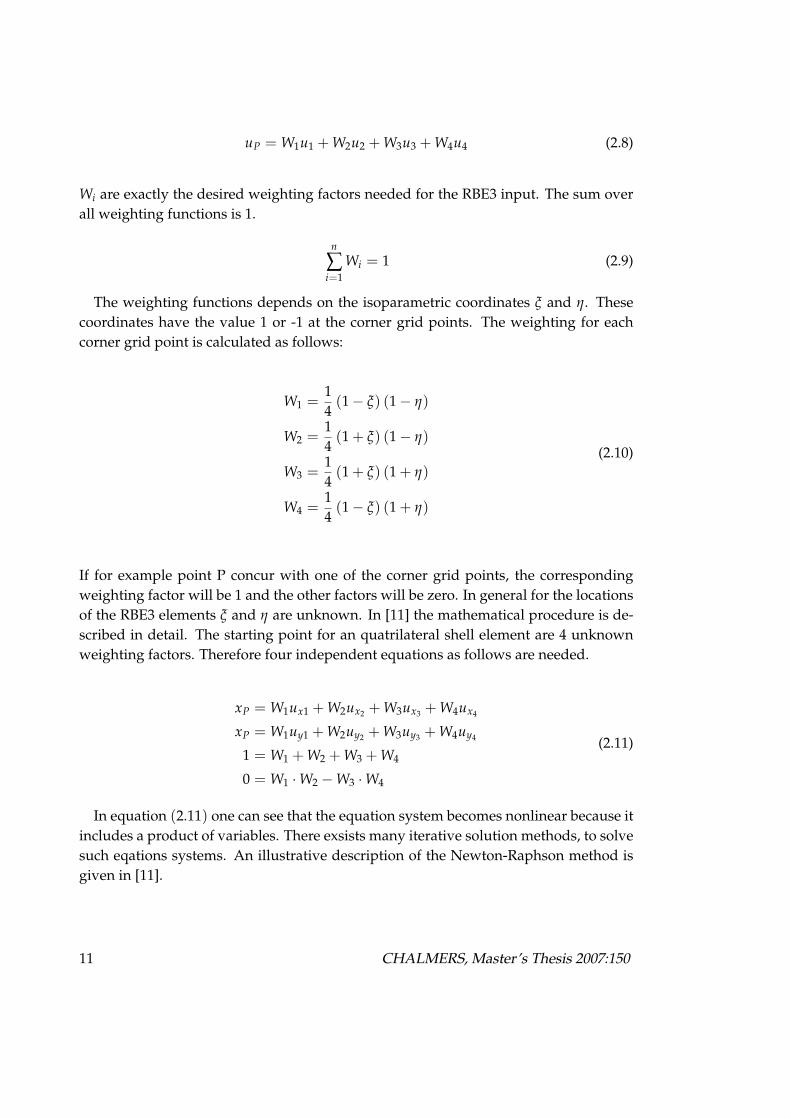
uP = W1u1 + W2u2 + W3u3 + W4u4 (2.8)

Wi are exactly the desired weighting factors needed for the RBE3 input. The sum overall weighting functions is 1.

n

!i=1

Wi = 1 (2.9)

The weighting functions depends on the isoparametric coordinates ! and ". Thesecoordinates have the value 1 or -1 at the corner grid points. The weighting for eachcorner grid point is calculated as follows:

W1 =14

(1" !) (1" ")

W2 =14

(1 + !) (1" ")

W3 =14

(1 + !) (1 + ")

W4 =14

(1" !) (1 + ")

(2.10)

If for example point P concur with one of the corner grid points, the correspondingweighting factor will be 1 and the other factors will be zero. In general for the locationsof the RBE3 elements ! and " are unknown. In [11] the mathematical procedure is de-scribed in detail. The starting point for an quatrilateral shell element are 4 unknownweighting factors. Therefore four independent equations as follows are needed.

xP = W1ux1 + W2ux2 + W3ux3 + W4ux4

xP = W1uy1 + W2uy2 + W3uy3 + W4uy4

1 = W1 + W2 + W3 + W4

0 = W1 · W2 "W3 · W4

(2.11)

In equation (2.11) one can see that the equation system becomes nonlinear because itincludes a product of variables. There exsists many iterative solution methods, to solvesuch eqations systems. An illustrative description of the Newton-Raphson method isgiven in [11].


The area of the brick element corresponds like for the CWELD model to the equiv-alent cross section area of the real spot weld. Figure (2.7) illustrates, how the size a ofthe brick element is related to the real spot weld.

Figure 2.7: The equivalet cross section area of the brick element

With the given diameter D of the real spot welds on the structure the size a of thehexa element will be calculated with following equation

a =-

%d2

4(2.12)

In Pre-processors like ANSA there is a possibility to enlarge the size of a brick ele-ment with the help of a so-called area factor (af). This factor enlarges the area of a hexaelement with a factor multiplied to the origin area. If for example the area factor hasthe value 3, the size of the brick element corresponds to that length needed to increasethe cross section area of the hexa element 3 times the origin one.

An important fact is that the weighting procedure depending on the linear shapefunction ensures that the center of highest stiffness is always in the center of the brickelement regardless of its location in the mesh. Due to the fact that the center node isconnected with all 4 corner nodes of the brick element it acquires the strongest couplingwith the brick element. The weighting factor depending on the shape function of allthe connected shell elements constructs a “stiffness near field”which radiates on thecoupled patch area like drawn in figure (2.8). So we can assume the near field aroundthe spot weld as a monopol with an equal stiffness distribution in all directions.


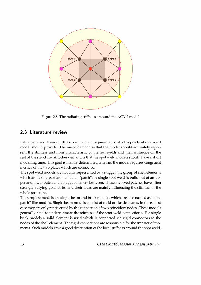
Figure 2.8: The radiating stiffness araound the ACM2 model

2.3 Literature review

Palmonella and Friswell [01, 06] define main requirements which a practical spot weldmodel should provide. The major demand is that the model should accurately repre-sent the stiffness and mass characteristic of the real welds and their influence on therest of the structure. Another demand is that the spot weld models should have a shortmodelling time. This goal is mainly determined whether the model requires congruentmeshes of the two plates which are connected.The spot weld models are not only represented by a nugget, the group of shell elementswhich are taking part are named as ”patch”. A single spot weld is build out of an up-per and lower patch and a nugget element between. These involved patches have oftenstrongly varying geometries and their areas are mainly influencing the stiffness of thewhole structure.The simplest models are single beam and brick models, which are also named as ”non-patch” like models. Single beam models consist of rigid or elastic beams, in the easiestcase they are only represented by the connection of two coincident nodes. These modelsgenerally tend to underestimate the stiffness of the spot weld connections. For singlebrick models a solid element is used which is connected via rigid connectors to thenodes of the shell element. The rigid connections are responsible for the transfer of mo-ments. Such models gave a good description of the local stiffness around the spot weld,


but they don’t have suitable parameters for an updating process. But the main disad-vantage of single beam and brick models are that non-congruently meshes couldn’t beconnected. So it is necessary to remesh around the spot weld center, which violateswith the goal of a fast modelling time.The most common spot weld approaches in NVH [01] are the ACM2 (area contactmodel 2) and the CWELD model. The ACM2 model is proposed from Heiserer et al.[03] it consist of a brick element which is connected via RBE3 elements with the up-per and lower plate. The element is available in MSC.Nastran as well as the CWELDmodelling approach. The CWELD has instead of a brick element for the nugget repre-sentation a special shear flexible beam-type element, with two nodes and 12 degrees offreedom (DOF). The 6 DOF’s of the two beam ends are connected with shell nodes ofthe participated plates and form a patch.In [01, 06] the spot weld models mentioned above were used to investigate sensitive pa-rameters, which can be used to update and validate the finite element approaches. Forthis purpose a benchmark structure was constructed to achieve experimental data forthe updating process. The benchmark structures have been a ”single and a double hat”construction, which are steel plates who have in the cross section a form like a ”hat”.These plates are joined together at the flanges to represent for example a roof pillar ofcar body. The general intention of the approach in [01, 06] is to use measurement data ofthe benchmark structure to determine values of appropriate stiffness parameter. Firstthe separate plates were tested and updated, so that the error which might occur in thewelded structure is only due to the spot weld model itself. The benchmark structure isthen updated only with the use of parameters which are involved in the spot weld ap-proach. The investigated parameters are the patch area (PA), the patch size (PS, whichis the square root of the area), the patch Young’s modulus (PE), the spot diameter (SD)and the spot Young’s modulus (SE).The updating in [01] is performed with an optimisation algorithm implemented in theFE-code MSC.Nastran. The code specifies an objective function which is minimised andinfluences the output variables of the FE-analysis. In the present study only the eigen-frequencies are regarded and the objective function is described in [17].In [01] it’s shown that for the CWELD and the ACM2 model PA and PE are sensitiveparameters and for the ACM2 additionally the spot diameter. In a common FE-modelthe patch has the same Young’s modulus like the surrounded structure (i.e. for steel 210GPa). The PA is dependent on the mesh size of the involved panels and SD is normallyequal with the real nugget diameter. Palmonella [18] found out in experimental teststhat the spot weld diameter doesn’t influence the dynamic behaviour of the structureand therefore the eigenfrequencies. For CWELD and ACM2 an optimal patch size be-tween 9 and 12 mm was shown. The assumption to use PE for compensation of notideal patch size does only hold up to a PS of 12 mm, above PE and PS have differ-ent influence on the eigenfrequencies. For small values of PS the updating of PE leads


to a decreasing difference between measured and calculated natural frequencies. Butsmaller patch sizes reduce the sensitivity of the eigenfrequencies to the patch parame-ter, which requires very large variations of the patch Young’s modulus in the updatingprocess.In real structures the spot welds are mostly grouped in rows. Thus one can define twodirections, one is ”longitudinal” which refers to the direction parallel to the spot weldrow, the second direction is ”transverse” and perpendicular to the spot welds line. Testsin [01] show clearly that parameters like patch width, position of the spot weld, patchand spot shifts related to the transverse direction are much more important than inlongitudinal direction. The reason is that the transverse direction significantly effectsthe stiffness property and hence the dynamic behaviour of the structure. Another notunimportant parameter is the thickness of the plates, which show up in the patch ofthe spot element. For variations in plate thickness the ACM2 model is a little bit lesssensitive than the CEWLD.In [01] a guideline is given for the CWELD and ACM2 models how to update them andminimise the difference between measured and calculated eigenfrequencies. For differ-ent plate thicknesses a optimum patch size (PS) is presented and the percentage changein the patch Young’s modulus (PE) if below or above optimum PS. Using this updatingapproach for the ”single and double hat” structure welded with ACM2 and CWELD,the errors in the first 10 eigenfrequencies can be reduced in average to less than around2%.


3 The benchmark structures

To produce experimental data which is necessary to validate the corresponding Finite-Element-models a suitable benchmark structure is needed. In this work the benchmarkstructure is a sidemember panel from a current Volvo car body. The sidemember is abearing part in the engine compartment which has a large importance for crash safety.Therefore the sidemembers represent a quite stiff structure of the car with a nominalpanel thickness between 1.8 and 2.0 mm. The complete sidemember installed in the caris built up with a so called inner sidemember and the corresponding outer part, whichare both shown in pictures (3.1, 3.2).The sidemembers are pressed metal panels which have a complex three dimensionalshape with holes and curvatures. Both panels have dimensions in the width directionof ca. 21 cm at the short side and of ca. 54 cm at the long side. The inner and outersidemembers have a length of approx. 109 cm and 84 cm.

Figure 3.1: Single inner sidemember

17

Figure 3.2: Single outer sidemember

To form the sidemember ”assembly” the outer panel is put on the top of the innerpart, with the positions like demonstrated in the pictures (3.1, 3.2). The inner and outersidemember panels are welded together with 49 spot welds which have a nominal di-ameter of 6 mm. The spot welds are positioned along the flanges of the assembledsidemember, which can be depicted in figure (3.3).

Figure 3.3: Welded sidemember (assembly)


4 Measurements

For validation purpose of the Finite-Element-models vibration measurements were per-formed with the use of the benchmark structure described in chapter (3).

4.1 Pre-Investigations

Based on the fact that the single sidemember panels and the welded assembly representa very stiff test specimen investigations are done to find suitable excitation points on theobjects. Due to this reason eigenfrequency analyses of the three different sidememberparts are made with MSC.Nastran. The calculated eigenfrequencies and eigenvectorsare used to animate the related mode shapes in Matlab. With the help of these modeshape animations the areas with the highest displacements on the test objects are de-termined. These ”sensitive” regions are used for the placement of excitation points tomeasure frequency response functions (FRF’s). For all three sidemember parts the exci-tation points are later placed mainly on the flanges of the structures, because there thelargest movements can be observed for the majority of the modes. This can be seen inthe figures (4.1, 4.2) as an example for the mode shapes of the first eigenfrequency.

Figure 4.1: Mode shapes of the first eigenfrequency for the inner sidemember (left) andouter sidemember (right)

19

Figure 4.2: Mode shape of the first eigenfrequency for the welded assembly

4.2 Configuration

After the excitation points were chosen, the structure under investigation was hookedup with springs to achieve free-free conditions, which can be seen in picture (4.3). Theexcitation was done with a shaker which was connected via a stinger to the test object.All specimens were excited from the bottom side, so that the responses could be mea-sured at the facing positions on the upper side. At five measurement points on eachsidemember panel the Pointmobilities (PMOB) and the belonging Transfermobilities(TFMOB) were determined to get a complete FRF-matrix. All measurements were car-ried out in the frequency range between 0 and 1000 Hz and with the highest frequencyresolution, which is available from the acquisition system. This is necessary to achievea sufficient resolution especially at the resonances peaks of these very light dampedstructures.


Figure 4.3: Measurement Set-Up

4.3 Eigenfrequencies & Damping

The measured mobility’s, like described in (4.2), were used to determine the eigen-frequencies and the modal damping of the sidemember parts. For this purpose theComplex Exponential Method was selected, like described in [13]. The viscous damp-ing factor (!r) was transferred in the loss factor ("r) to have later an estimation valuefor the Direct Frequency Response Analysis in MSC.Nastran. But the main focus in thiswork was set on the determination of the eigenfrequencies from measurements. Withthe use of the measured Pointmobilities the eigenfrequencies were extracted. For eachsidemember set with three specimens an averaging process was performed, to obtain”mean” eigenfrequencies for the inner & outer sidemembers and the welded assembly.These ”mean” measured eigenfrequencies will be compared later in this work directlywith the FE-simulations. In table (4.1) the ”mean” eigenfrequencies are presented forthe inner & outer sidemember and the welded assembly.


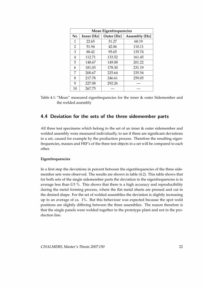
Mean EigenfrequenciesNr. Inner [Hz] Outer [Hz] Assembly [Hz]1 22.65 31.27 68.192 51.94 42.06 110.113 88.42 95.65 135.744 112.71 133.52 161.455 148.67 149.08 201.226 181.03 178.30 231.197 200.67 225.64 235.548 217.78 246.61 259.059 227.08 292.26 —10 267.75 — —

Table 4.1: ”Mean” measured eigenfrequencies for the inner & outer Sidemember andthe welded assembly

4.4 Deviation for the sets of the three sidemember parts

All three test specimens which belong to the set of an inner & outer sidemember andwelded assembly were measured individually, to see if there are significant deviationsin a set, caused for example by the production process. Therefore the resulting eigen-frequencies, masses and FRF’s of the three test objects in a set will be compared to eachother.

Eigenfrequencies

In a first step the deviations in percent between the eigenfrequencies of the three side-member sets were observed. The results are shown in table (4.2). This table shows thatfor both sets of the single sidemember parts the deviation in the eigenfrequencies is inaverage less than 0.5 %. This shows that there is a high accuracy and reproducibilityduring the metal forming process, where the flat metal sheets are pressed and cut inthe desired shape. For the set of welded assemblies the deviation is slightly increasingup to an average of ca. 1%. But this behaviour was expected because the spot weldpositions are slightly differing between the three assemblies. The reason therefore isthat the single panels were welded together in the prototype plant and not in the pro-duction line.


Deviation in EigenfrequenciesNr. Inner [%] Outer [%] Assembly [%]1 0.3 0.4 1.32 0.3 0.3 0.33 0.1 0.1 1.24 0.1 0.1 0.95 0.1 0.2 1.06 0.4 0.3 0.27 0.2 0.1 0.88 0.5 0.3 1.19 1.0 0.2 —10 0.1 — —

Table 4.2: Deviation in eigenfrequencies for the sets of inner & outer sidemember andthe welded assembly

Masses

In a next step the ”real” mass of each panel or assembly was determined to see thelargest deviation in each set of the three sidemember parts. The results are presented intable (4.3), where one can observe that the maximum deviation is less than 22 g for allthree sidemember sets.

Outer Panel 1 4.342 kgPanel 2 4.350 kgPanel 3 4.349 kg

max. deviation 8 gInner Panel 1 6.277 kg

Panel 2 6.293 kgPanel 3 6.295 kg

max. deviation 18 gWelded Assembly 1 10.625 kg

Assembly 2 10.647 kgAssembly 3 10.639 kg

max. deviation 22 g

Table 4.3: Deviation in mass for the sets of inner & outer Sidemember and the weldedassembly


Annother interesting comparison is presented in table (4.4). There the measuredmasses of all three inner and outer sidemembers were summed up and compared withthe corresponding measured masses of the assemblies. The resulting differences indi-cate that the welding process itself didn’t influence the mass of the structures signifi-cantly. These small mass deviations are negligible and confirm with the observationsmade for the eigenfrequencies.

assembly measured [kg] measured [kg] sum measured [kg] diffsidemember inner sidemember outer [kg] welded assembly [g]

1 6,277 4,342 10,619 10,6245 5,52 6,293 4,350 10,643 10,6469 3,93 6,295 4,349 10,644 10,6391 -4,9

Table 4.4: Comparison of mass deviation after welding process

FRF’s

To see if there are significant deviations over the entire frequency range of interest,measured FRF curves were compared.

0 100 200 300 400 500 600 700 800 900 1000−160

−140

−120

−100

−80

−60

−40

frequency f [Hz]

leve

l [dB

re. 1

mm

/Ns]

Inner 01 PMOB H_11Inner 02 PMOB H_11Inner 03 PMOB H_11

Figure 4.4: Comparison of Pointmobilities of the inner sidemember

As representative examples the Pointmobilities of the inner sidemembers at measure-


ment point 1 and of the welded assemblies at measurement point 3 were chosen, whichare illustrated in figures (4.4) and (4.5). There it gets obvious that all three Pointmobilitycurves show only small differences, even up to 1000 Hz.

100 200 300 400 500 600 700 800 900 1000−120

−100

−80

−60

−40

−20

0

20

Frequency [Hz]

Mob

ility

[dB

re. 1

m/N

s]

Assembly 01 PMOB H_33Assembly 02 PMOB H_33Assembly 03 PMOB H_33

Figure 4.5: Comparison of the measured point mobility on all individual assemblies

These insignificantly deviations in eigenfrequencies, masses and FRF’s in each setof the three sidemember parts are a indicator for the precision during the productionprocess and just so for the performed measurements. This confirms the procedure todetermine ”mean” eigenfrequencies for each set of the sidemember parts and to calcu-late also a mean FRF for comparison with the corresponding FE-calculations.


5 Single sidemember panels

In this chapter measured FRF curves and eigenfrequencies of the single sidememberpanels will be compared with the relevant FE-simulations. The FE-calculations wereperformed with the FE-solver of MSC.Nastran. For the calculation of the eigenfrequen-cies the Real Eigenvalue Extraction was chosen, which uses the Lanczos Method andis defined with the solution number SOL 103 in MSC.Nastran. The frequency responseanalysis was done with the Modal Frequency Response Method, which is selected withSOL 111. Both solution methods are described in detail in the Basic Dynamic Analysismanual [20] of MSC.Nastran.The sidemember panels were modelled with shell elements, using exclusively quadri-lateral plate elements and in some small areas triangular shell elements. These areCQUAD4 and CTRIA3 elements in MSC.Nastran 2005 and described in the Quick Ref-erence Guide [20].

5.1 Mesh refinement

All following investigations concerning the single sidemember panels are described ex-emplarily with the inner sidemember because the results for the outer panel are mainlyidentical. If there are any significant differences occurring, explicit statements will bemade.At the moment the quadrilateral elements have a ”standard” mesh size of 10 mm and alinear shape function. At this point it should be stated that one of course can use higherorder shape functions instead of refining the mesh to achieve the same or similar effect.But in the automotive industry it is usual to use the same meshes for Durability, Crashand NVH to safe time and costs. Especially for crash simulations linear shape functionsare absolute necessary, so that they have to be used for NVH purpose as well. In thiswork the 10 mm mesh is the ”reference size” and in addition three smaller mesh sizeswere investigated, which are 5, 2.5 and 1 mm. The inner sidemember panels have twoareas with a nominal thickness distribution of 1.8 and 2.0 mm.In figure (5.1) one can see for the inner panel the FE-calculations for the 10 and 1 mmmesh and the corresponding mean measured curve. There it gets obvious that it is hardto recognize the differences in eigenfrequencies in such a FRF plot.

27

0 50 100 150 200 250 300−160

−140

−120

−100

−80

−60

−40

Frequency [Hz]

Leve

l [dB

re. 1

mm

/Ns]

Sidemember inner − nominal thickness −

H11 10 mm meshH11 1 mm meshH11 mean measured

Figure 5.1: Moblity curves for the inner sidememeber with a mesh size of 10 and 1 mmand the corresponding mean measured curve

Even for the largest difference between 10 and 1 mm and a reduced frequency rangefrom 0 to 300 Hz, it’s necessary to zoom in a single resonance to detect differences.This way of graphical presentation is shown in figure (5.2) exemplary for the resonancefrequency at around 150 Hz and all used mesh sizes. But even with this extensive pro-cedure it’s almost impossible to make these small differences visible, so it was decidedto chose for further comparisons a bar plot which shows the differences in percent be-tween FE-calculations and measurements for all modes up to 300 Hz. Such a bar plot isillustrated in figure (5.3) for the inner sidemember. There one can now clearly see thedeviation between measurement and FE-calculation for the first ten modes of the innerpanel. With this kind of graphic the influence of each mesh refinement step can be de-tected and the efficiency estimated. For the inner panel the first mesh refinement from10 down to 5 mm shows the largest effect and the improvement for the first ten modesis in average around 0.5%. Looking on the same graphic for the outer sidemember infigure (A.1) of the appendix, one can see for the same refinement step from 10 to 5 mma larger improvement than for the inner panel.


146 148 150 152 154 156 158

−82

−80

−78

−76

−74

−72

−70

−68

−66

Frequency [Hz]

Leve

l [dB

re. 1

mm

/Ns]


H11 10 mm meshH11 5 mm meshH11 2.5 mm meshH11 1 mm meshH11 mean measured

Figure 5.2: Zoom view of a resonance frequency at around 150 Hz

1 2 3 4 5 6 7 8 9 100

1

2

3

4

5

6

7

8

mode number

diffe

renc

e to

mea

sure

men

t [%

]


10 mm mesh 5 mm mesh 2.5 mm mesh 1 mm mesh

Figure 5.3: Differences in eigenfrequencies for the first ten modes of the inner sidemem-ber, due to mesh refinement

To make the influence of this first refinement step more visible, the arising differencein Hz due to refinement is plotted for a larger frequency range up to around 750 Hz


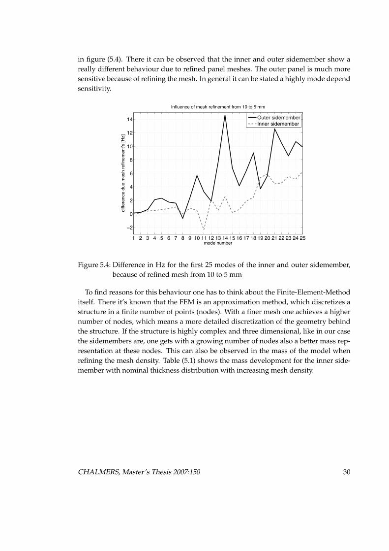
in figure (5.4). There it can be observed that the inner and outer sidemember show areally different behaviour due to refined panel meshes. The outer panel is much moresensitive because of refining the mesh. In general it can be stated a highly mode dependsensitivity.

1 2 3 4 5 6 7 8 9 10 11 12 13 14 15 16 17 18 19 20 21 22 23 24 25

−2

0

2

4

6

8

10

12

14

mode number

diffe

renc

e du

e m

esh

refin

emen

t’s [H

z]

Influence of mesh refinement from 10 to 5 mm

Outer sidememberInner sidemember

Figure 5.4: Difference in Hz for the first 25 modes of the inner and outer sidemember,because of refined mesh from 10 to 5 mm

To find reasons for this behaviour one has to think about the Finite-Element-Methoditself. There it’s known that the FEM is an approximation method, which discretizes astructure in a finite number of points (nodes). With a finer mesh one achieves a highernumber of nodes, which means a more detailed discretization of the geometry behindthe structure. If the structure is highly complex and three dimensional, like in our casethe sidemembers are, one gets with a growing number of nodes also a better mass rep-resentation at these nodes. This can also be observed in the mass of the model whenrefining the mesh density. Table (5.1) shows the mass development for the inner side-member with nominal thickness distribution with increasing mesh density.


Inner sidemember mass development [kg]mesh density 10 mm 5 mm 2.5 mm 1 mm

nominal 6,712 6,730 6,734 6,736measured 6,288 6,288 6,288 6,288Difference 0,423 0,442 0,446 0,447

Table 5.1: Mass development when refining the mesh density with nominal thickness

It can be seen that the increasing mesh density leads to an small increasing mass ofabout 24 g because of a better approximation of geometry (curvatures and holes). Thisat least results in a small drop in eigenfrequencies. The mass then directly influence thecalculation of the eigenfrequencies and the mode shapes, which are moving nearer tothe measured (”reference”) values. In figure (5.4) one can observe that the convergencestep of the eigenfrequencies to the ”real” value is stronger with growing frequency. Areason therefore is that with higher frequencies and shorter wavelength fine details ingeometry, like small holes and edges, affect stronger the vibrational properties of thestructure. In figure (5.5) the same geometry area is shown, once with the standard meshsize of 10 mm and then with the finer mesh size of 2.5 mm. There the effect of the bettergeometry approximation gets directly visible. At the end the change of the consideredeigenfrequency due to a refined panel mesh depends only on how good the standardmesh could represent the geometry and the occurring bending stiffness at this specificfrequency under investigation.For the single inner and outer sidemember panels the first refinement step from 10 to 5mm has the largest effect in reducing the deviation between measured and calculatedeigenfrequencies. With this first step an improvement in the eigenfrequencies of ca.0.5% could be achieved for the first ten modes. Both next refinement steps from 5 to 2.5mm and 2.5 to 1 mm, change the eigenfrequencies in average only about 0.1%.


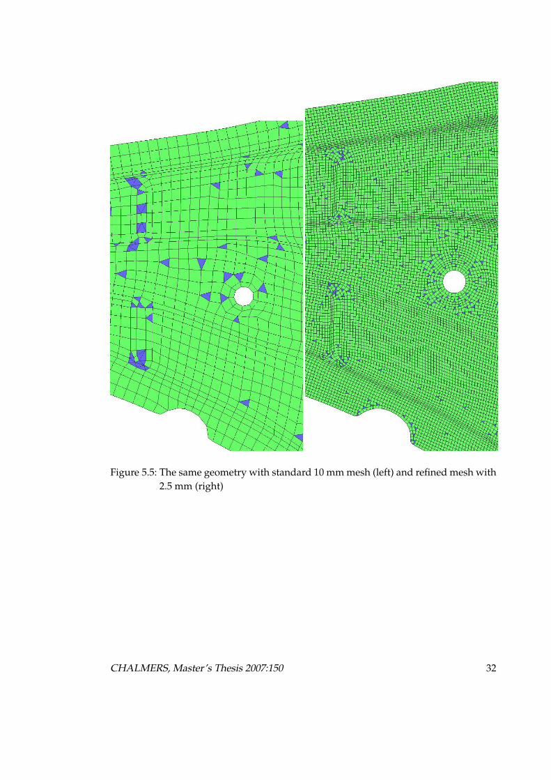
Figure 5.5: The same geometry with standard 10 mm mesh (left) and refined mesh with2.5 mm (right)


5.2 Mapped thickness distribution

After refining the mesh size a detailed thickness distribution over the surface of thepanels was tested. This detailed thickness information’s come from the metal formingprocess where the originally flat metal sheet is pressed in the desired shape. To exam-ine this pressing process also FE-simulations are performed, to check that no possiblefracture zones appear. These metal forming simulations contain the actual height of thepanel at each node.

In figure (5.6) such a mapped thickness is presented for the inner sidemember panel.There it can be seen that the inner panel has two parts with different initial heights.The left side has a starting height of 1.8 mm and the right side of 2.0 mm. Due to thepressing process the maximum height difference can be more than 0.5 mm on this sin-gle panel. It is also possible that the thickness of some areas increase above the initialheight because the metal moves under the high pressure; like for the right side of theinner panel. But over the whole panel a noticeable variation in height gets visible.

Figure 5.6: Mapped thickness distribution for the inner sidemember


Previous FE-simulations neglected this existing effect of mapped thickness. In thefollowing FE-calculations the mapped thickness was implemented into the presentmeshes, to see how they influence the dynamic properties of the sidemember parts.

In figure (5.7) the 10 mm standard mesh is compared with nominal and mapped thick-ness, additionally the mesh refinements of 5 and 2.5 mm for the mapped thicknessare illustrated. There it gets obvious that with the consideration of the real thicknessthe deviation in eigenfrequencies between measurement and FE-calculation can be re-duced in average for the first ten modes of the inner panel by ca. 3%. The expecteddifferences due mesh refinement appear in the same order as for the nominal thickness.Now the question came up, what are the reasons for such a large improvement causedby mapping.

1 2 3 4 5 6 7 8 9 100

1

2

3

4

5

6

7

mode number

diffe

renc

e to

mea

sure

men

t [%

]

Sidemember inner − influence of mapped thickness −

10 mm mesh − nominal thickness 10 mm mesh − mapped thickness 5 mm mesh − mapped thickness 2.5 mm mesh − mapped thickness

Figure 5.7: Comparison of eigenfrequencies with nominal and mapped thickness forthe inner sidemember

First the mass development of the FE-models for the inner sidemember was investi-gated, like shown in table (5.2).


Inner sidemember mass development [kg]mesh density 10 mm 5 mm 2.5 mm 1 mm

mapped 6,311 6,331 6,336 6,338measured 6,288 6,288 6,288 6,288Difference 0,023 0,043 0,048 0,050

Table 5.2: Mass development when refining the mesh density with mapped thickness

There one could find a mass reduction of 373 g between the 10 mm standard modelwith nominal thickness and the 1 mm mapped model. The mass of the models is con-verging down and is with the 1 mm mapped model only 50 g above the ”real” weightedmass. Generally a decreasing mass leads to increasing eigenfrequencies, but figure (5.7)shows the opposite behaviour. If not the change in mass is responsible for the shifteddownwards eigenfrequencies, it has to be the changed thickness itself. Therefore thebehaviour of the bending wavelength for a simple quadratic plate was chosen, whichcan be calculated like follows:

&B = 2 · % 4

.E · h3

12 (1" µ2) · m# · '2 (5.1a)

&B = 2 · % 4

.E · h3

12 (1" µ2) · h · ( · '2 (5.1b)

With equation (5.1b) two cases were calculated, first reducing the thickness of the platefrom 2.2 mm down to 1.7 mm and then changing the density to achieve the same massreduction like with the reduced thickness by 0.5 mm. The resulting changes in fre-quency for three observed frequency points are presented in table (5.3).

observed "f [Hz] when "f [Hz] whenfrequency points changing changing

[Hz] thickness h density (

200 -45 28400 -81 55600 -136 83

Table 5.3: Frequency steps due to changing thickness or density

There it gets evident if changing the thickness the eigenfrequencies are decreasingand the plate becomes ”weaker”. If adjusting the density a ”stiffening” of the plateis visible and the eigenfrequencies are increasing. If simplifying equation (5.1b), with


eliminating the thickness in the denominator, which comes from the calculation of themass per area, the thickness in the numerator has still the power of two. So it is ob-vious that for the bending wavelength and therefore also for the eigenfrequencies thethickness of the structure is the dominating parameter. With these mapped thicknessdistribution one gets a much better representation of the reality than with using a nom-inal thickness over the whole panel area. And since the thickness of a structure is dom-inating its bending stiffness behaviour, the deviation between measured and calculatedeigenfrequencies can be reduced significantly with the use of mapping. This gets alsovisible when comparing FRF curves, like in figure (5.8). There one can see a directcomparison between nominal and mapped thickness distribution and as a referencethe corresponding measured curve. With growing frequency the improvement due tomapping gets larger, which is detailed illustrated for an extended frequency range inthe appendix (A.2).

0 50 100 150 200 250 300−150

−140

−130

−120

−110

−100

−90

−80

−70

−60

−50

Frequency [Hz]

Leve

l [dB

re. 1

mm

/Ns]

Sidemember inner − Influence of mapped thickness −

H11 10 mm mesh nominalH11 10 mm mesh mappedH11 Mean measured

Figure 5.8: FRF comparison to show the influence of mapping


5.3 Main results

To improve the FE-model with the complex geometry of the single sidemember pan-els a mapped thickness distribution was introduced. This leads to a reduction of thedeviation between measured and calculated eigenfrequencies of ca. 3%. In contrastto a simple Young’s Modulus updating, the improvement due mapping works nearlyuniformly for all modes in the frequency range up to 300 Hz. The mapped thickness re-duces the error between eigenfrequencies from measurements and FE-simulations forthe first ten modes of the single sidemember panels to less than 2% in average.

In another investigation the standard mesh size of 10 mm was refined down to 5, 2.5and 1 mm. To see the influence of this three refinement steps, the change of the eigenfre-quencies in Hz for the inner and outer sidemember was averaged and plotted in figure(5.9) for the first 25 modes, which cover a frequency range from 0 up to ca. 750 Hz.

1 2 3 4 5 6 7 8 9 10 11 12 13 14 15 16 17 18 19 20 21 22 23 24 25−1

0

1

2

3

4

5

6

7

8

9

10

mode number

diffe

renc

e du

e m

esh

refin

emen

t’s [H

z]

Influence of mesh refinements for mean Inner & Outer sidemembers

mesh refinement 10 to 5 mm mesh refinement 5 to 2.5 mm mesh refinement 2.5 mm to 1 mm

Figure 5.9: Change of eigenfrequencies in Hz for all three refinement steps

An interesting observation is that a few modes show a strong reaction or are insen-sible at all in consequence to a finer mesh. Insensibility means that the ”rough” meshwas already sufficient to describe this single mode. Instead a strong reaction shows the


requirement of finer mesh size. But in general the largest improvement can be achievedwith the step from 10 to 5 mm mesh size.Up to 300 Hz this leads to an improvement of the FE-calculated eigenfrequencies of ca.0.5%, but the tendency is that the improvement increases with frequency. So it dependson the frequency range of interest if the refinement from 5 to 2.5 mm is useful or not.The refinement step from 2.5 mm to 1 mm changes the eigenfrequencies only about 1Hz for all 25 modes under investigation, but the calculation effort is increasing expo-nentially. So this case, with refining the panel mesh down to 1 mm is inefficient and notrecommendable.


6 Investigations of welded assembly

After the investigations on the single sidemember parts, the welded structure has tobe modeled. Due to the welding process the global stiffness of the assembly is nowdetermined by the bending stiffness of each single members but mainly of the stiffnessof the spot weld connections [07]. After joining the single side members together, theexact spot weld positions were determined with the help of a special laser system forall three assemblies. With the laser measurement data it is possible to implement thespot weld models in the FEM model exactly at the same position. In figure (6.1) one cansee the 49 spot weld positions which are marked as black square elements.

Figure 6.1: FEM model of welded assembly with black marked spot weld positions

39

6.1 ACM2 vs. CWELD

As mentioned in [05] the most widely used spot weld models in industry are the ACM2and CWELD model. In a first investigation simulations with both models have beencarried out to be able to compare the performance of both models concerning to furthermesh refinement. Therfore the standard models with an spotweld diameter of 6 mmhave been used. Figure (6.2) shows the results for mesh refinement steps from 10 mmdown to 2.5 mm.

1 2 3 4 5 6 7 8 9−8

−6

−4

−2

0

2

4

6

8

mode number

diffe

renc

e to

mea

sure

men

t [%

]

Welded assembly − nominal tickness −

10 mm mesh CWELD PARTPAT 10 mm mesh ACM2 area factor 1 5 mm mesh CWELD PARTPAT 5 mm mesh ACM2 area factor 1 2.5 mm mesh CWELD PARTPAT 2.5 mm mesh ACM2 area factor 1

Figure 6.2: Difference between measured and calculated natural frequency for the dif-ferent models [%]

With a 10 mm mesh the CWELD and the ACM2 model performs quite similar. Whengoing down to 5 mm mesh size the CWELD model begins to loose more stiffness espe-cially at mode number 3 and 4. Here the ratio D/S becomes larger 1 which leads to anunderestimation of the connection stiffness. This effect becomes larger with a meshsizeof 2.5 mm. But there occured also an another difficulty. Due to the fact that the CWELDmodel is only able to connect from 1 up to 3x3 shell elements, the spotweld diame-ter has also to be reduced. Now a second factor, the spot weld diameter additionallyinfluences the connection stiffness.


As mentioned in [01] the spot weld diameter is not a sensitive parameter for theCWELD model, but decreasing the diameter includes also a reduction of the connectedpatch area, especially at small mesh sizes. The patch area again is of course a sensitiveparameter as well as for the ACM2 model.

Although both models loose stiffness with further mesh refinement, the CWELDmodel performs worse because of its functional limitations. It becomes clear that tocompensate the loss in bending stiffness due to mesh refinement the CWELD will bemore difficult to control. This is mainly because the only sensitive parameter in thePWELD entry which is possible to change, is the spot weld diameter. This shows thatin general the CWELD model is not applicable for mesh sizes smaller than 5 mm. As aconsequence further investigations have been done with the ACM2 model.

6.2 ACM2 model

As mentioned in chapter (1) the ACM2 model leads to a drop of global stiffness in theFEM calculation when refining the meshsize. The difficulty on the current model is ofcourse that further mesh refinement itself leads as well to a drop of stiffness because ofthe better approximation of geometry. The coarsest mesh size for all investigations is a10 mm mesh. Therefore it is important to find out an optimal spot weld configuration,which doesn’t introduce any additional error in the simulation results. With a 10mmmesh the simulation results from the single sidemembers with nominal thickness haveshown at the first 8 mode numbers a mean deviation of approximately 5 %. Normallythe same quantity should also occur on the welded assembly with 10 mm mesh, if theapplied spotweld model doesn’t introduce any significant error from the beginning. In[01] Palmonella stated following sensitive parameters for the ACM2 model:

• Patch area (the area which encircles all connected shell elements)

• Patch Young’s modulus

• Spot weld diameter (size of the brick element)

The patch area depends from the used mesh density, the Patch Young’s modulus isnot really a parameter which is practical to change, because the amount of elementswhich have to be updated changes with the used mesh density. The easiest possibilityis to change the brick dimensions (spot weld diameter), because this parameter is meshindependent. To find out the optimal ACM2 configuration for a 10 mm mesh, severalarea factors have been investigated.


1 2 3 4 5 6 7 8 90

1

2

3

4

5

6

7

mode number

diffe

renc

e to

mea

sure

men

t [%

]

Comparison − nominal thickness −

assembly, ACM2, 10 mm mesh area factor 1assembly, ACM2, 10 mm mesh area factor 3Mean value for single Inner & Outer sidemember

Figure 6.3: Comparison of area factor 1 and 3 with the mean deviation of single panels

Figure (6.3) shows, that area factor 3 (af3) is the best choice where the differencebetween the mean deviation of the single panels and the welded assembly becomesminimal. With area factor 3 the spot weld diameter was increased from 6 mm up to 9mm. This configuration corresponds also to the standard model used at Volvo.

Of course there is still a difference between the welded assembly with af3 and thevalues of the single panels. One reason therefore is that the patch area of each indi-vidual ACM2 model is not the same on the panels. Wether on the whole panel nor theupper and the lower patch of one ACM2 model have the same patch area. One reasontherfore is, because due to the complex shape of the structure some shell elements aredistorted from their basic shape. Another reason is the location of the brick elementinside the mesh. The largest patch area arises if each corner node of the brick elementis lying in a separate shell element. Due to the complexity of the whole structure noideal condition is given for each spot weld model. This of course affects individuallythe local bending stiffness of the structure. One can guess that these local variationsin bending stiffness will more affect local base modes than global modes on the struc-ture. Perhaps a compensation of such effects is only possible when updating only theseACM2 models whose stiffness is mainly responsible for a particular mode. But this ef-fort would be too high in comparison to the achievable improvement.


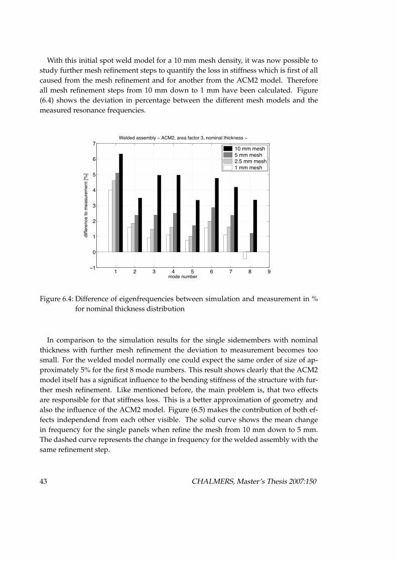
With this initial spot weld model for a 10 mm mesh density, it was now possible tostudy further mesh refinement steps to quantify the loss in stiffness which is first of allcaused from the mesh refinement and for another from the ACM2 model. Thereforeall mesh refinement steps from 10 mm down to 1 mm have been calculated. Figure(6.4) shows the deviation in percentage between the different mesh models and themeasured resonance frequencies.

1 2 3 4 5 6 7 8 9−1

0

1

2

3

4

5

6

7

mode number

diffe

renc

e to

mea

sure

men

t [%

]

Welded assembly − ACM2, area factor 3, nominal thickness −


Figure 6.4: Difference of eigenfrequencies between simulation and measurement in %for nominal thickness distribution

In comparison to the simulation results for the single sidemembers with nominalthickness with further mesh refinement the deviation to measurement becomes toosmall. For the welded model normally one could expect the same order of size of ap-proximately 5% for the first 8 mode numbers. This result shows clearly that the ACM2model itself has a significat influence to the bending stiffness of the structure with fur-ther mesh refinement. Like mentioned before, the main problem is, that two effectsare responsible for that stiffness loss. This is a better approximation of geometry andalso the influence of the ACM2 model. Figure (6.5) makes the contribution of both ef-fects independend from each other visible. The solid curve shows the mean changein frequency for the single panels when refine the mesh from 10 mm down to 5 mm.The dashed curve represents the change in frequency for the welded assembly with thesame refinement step.


0

5

10

15

diffe

renc

e [H

z]

Influence of ACM2 due mesh refinement − 10 mm to 5 mm −

Mean single Inner & Outer sidememeber Mean welded assembly − ACM2 −

1 2 3 4 5 6 7 8 9 10 11 12 13 14 15 16 17 18 19 20 21 22 23 24 25

0

2

4

6

mode number

diffe

renc

e [H

z]

Figure 6.5: Change in frequency with mesh refinement from 10 mm to 5 mm for the first25 mode numbers

One can see that the welded assembly shows a higher change in frequency like thesingle sidemembers. The area between both curves represents so to say the influencein frequency, for which only the ACM2 model is responsible for. The bar plot belowshows this difference for each mode number. It can be seen, that the influence of theACM2 models is mode dependend. This emphasizes the discussed influence of differ-ent patch areas of the individual ACM2 models to global and local modes.

Another investigation in [06] gives also a good explanation for mode dependency ofthis stiffness loss. There the different forces and moments acting at the spot welds havebeen analysed. It has been shown that a sensivity parameter like the patch area has thelargest influence to those modes where the push / pull forces and bending momentsare high in comparison to the shear forces. This means that the patch area has a largerstiffening effect to bending motion than for in-plane deformations. It is obviously thata reduction of the patch area by factor 4 due to mesh refinement has a higher affect tothe bending stiffness of the whole structure than to the shear stiffness.


6.3 Reasons for sti!ness loss with mesh refinement

To get a more detailed look on what happens, with further mesh refinement, one hasto observe a single ACM2 model in the welded assembly. In figure (6.6) there is drawna topview of an ACM2 model, before and after mesh refinement from 10 mm down to5 mm. It can be seen that with one refinement step the patch area is reduced by factor4. Another fact is, that the center of the brick element and thus the center of higheststiffness is not existing anymore, because the origin connection pattern of the wholeACM2 element is lost.

(a) origin ACM2 model (b) ACM2 model after mesh refinement

Figure 6.6: Topview of an ACM2 model when refining the mesh density from 10 mmdown to 5 mm

The answer for that lies in the implementation alghorithm for the ACM2 model.When connecting both sidemembers togehther the Pre-Processor tries to connect eachof all 4 RBE3 points with those shell elements the RBE3 points are lying inside. How-ever the originally ACM2 construction includes that not more than 4 shell elementsare falling inside the brick area. Otherwise the origin connection pattern of the cornernodes will be lost.


6.4 Influence of mapped thickness distribution

As the previous investigations on the single panels have shown, with mapped thicknessdistribution the mean deviation in percentage between the measured and calculatedresonance frequencies is about 2 % for the first 8 mode numbers. This means that wheneliminating the error introduced by the ACM2 model the applied mapped thicknessdistribution on the welded assembly the deviation to measurement should result inthe same order of size. Now the question arised, if the mapped thickness distributionhas the same influence on the welded structure. Because when both single membersare joined together a new structure arises and thus other geometrical properties couldovercome the influence of mapping. Therefore the same mesh refinement steps from 10mm to 1 mm have been calculated. In table (6.1) one can see the mass development forthe welded assembly for all mesh refinement steps. It shows clear that even the coarsestmesh size approximates the real mass of the structure quite well.

Assembly mass development [kg]mesh density 10 mm 5 mm 2.5 mm 1 mm

mapped 10,569 10,615 10,634 10,638´measured 10,637 10,637 10,637 10,637Difference -0,068 -0,022 -0,003 0,002

Table 6.1: Mass development for the assembly with mapped thickness

Figure (6.7) shows the deviation between the measured and the calculated resonancefrequencies. One can see that with further mesh refinement the calculated resonancefrequencies are now almost below the measured ones. This means that the structurebecomes too weak in comparison to the real one. In comparison to the nominal thick-ness distribution in figure (6.4) the mapped thickness distribution has still a significantinfluence even if the structure is joined together. But now the influence of the ACM2model is responsible for the fact that the bending stiffness of the FEM model is tooweak. Due to the fact that the mapped thickness distribution has still a positive effectto the calculation results, further investigation were carried out with mapped thicknessdistribution.


1 2 3 4 5 6 7 8 9−4

−3

−2

−1

0

1

2

3

4

mode number

diffe

renc

e to

mea

sure

men

t [%

]

Welded assembly − ACM2, area factor 3,mapped thickness −


Figure 6.7: Difference between calculated and measured natural frequency in % withmapped thickness distribution


6.5 ”RBE3 expansion” on ACM2 model

Based on a Matlab code written at Volvo, there is a possibility to expand the patch areaof an ACM2 spot weld model after mesh refinement. The programm needs a searchradius as an input parameter. The programm connects the RBE3 elements with all shellcorner nodes lying inside the given radius. The result of the expansion can be seen infigure (6.8).

Figure 6.8: ACM2 spot weld after expansion of connection nodes

To compensate the loss in patch area which is responsible for the loss of bendingstiffness it is necessary to know which search radius is the best one. Therefore differentmodels with different patch areas have been calculated. Figure (6.9) one can see theresult for different models where the search radius has been changed from 8 mm upto 15 mm. The thick solid curve represents the reference curve. This curve representsthe mean change in frequency for the single panels when refine the panel mesh from 10mm down to 5 mm.


1 2 3 4 5 6 7 8 9 10 11 12 13 14 15 16 17 18 19 20 21 22 23 24 25

−5

0

5

10

15

mode number

diffe

renc

e be

twee

n 10

and

5 m

m m

esh

[Hz]

ACM2 when expanding RBE3 connections − 10 to 5 mm mesh −

Mean single Inner & Outer sidememeber Welded assembly − ACM2, RBE3 expanded 8 mm − Welded assembly − ACM2, RBE3 expanded 10 mm − Welded assembly − ACM2, RBE3 expanded 12 mm − Welded assembly − ACM2, RBE3 expanded 15 mm −

Figure 6.9: Mean change in frequency with different search radius via ”RBE3 expan-sion” code for the first 25 mode numbers

One can see that a used search radius with 8 mm (dashed curve without markers)gives the smallest deflection to the reference curve. When increasing the patch areawith an 8 mm search radius after mesh refinement from 10mm to 5mm, the ACM2 in-fluence should nearly be eliminated. When now calculating the modified 5 mm and 2.5mm model the results in resonance frequency should show nearly the same steppingpattern in resonance frequency like for the single sidemembers. There the smallestmesh density should result in the smallest deviation to measurement. This is caused bythe better approximation of geometry should still remain in the same order like for thesingle panels. In figure (6.10) on can see the results for the first 8 mode numbers.The results show that the ”RBE3 expansion” increases the bending stiffness of the struc-ture but the stiffening effect is very inconstant over all mode numbers. Especially onthe first mode number the 2.5 mm model has now a larger bending stiffness like theorigin 10 mm model. On the second mode number the 5 mm model is the stiffest one.Thus the expected stepping is totally lost.


1 2 3 4 5 6 7 8 90

0.5

1

1.5

2

2.5

3

3.5

4

mode number

diffe

renc

e to

mea

sure

men

t [%

]

Welded assembly − ACM2, area factor 3,mapped thickness −

10 mm mesh 5 mm mesh RBE3 expansion 8 mm 2.5 mm mesh RBE3 expansion 8 mm

Figure 6.10: Deviation in % to measurement for refinement steps down to 2.5 mm meshdensity

A detailed look on the RBE3 entries gives a first answer on what happened. LikeFigure (6.6) shows, after applying the ”RBE3 expansion” code on the FEM model theRBE3 element is not only connected with four shell corner nodes like the original ACM2model. It rather connects all shell corner nodes lying inside the given search radius.

(a) origin ACM2 model (b) reconnected with ”RBE3 expansion”method


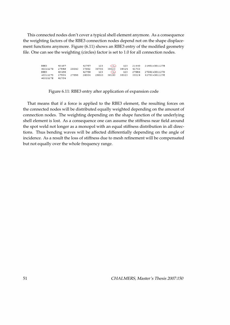
This connected nodes don’t cover a typical shell element anymore. As a consequencethe weighting factors of the RBE3 connection nodes depend not on the shape displace-ment functions anymore. Figure (6.11) shows an RBE3 entry of the modified geometryfile. One can see the weighting (circles) factor is set to 1.0 for all connection nodes.

Figure 6.11: RBE3 entry after application of expansion code

That means that if a force is applied to the RBE3 element, the resulting forces onthe connected nodes will be distributed equally weighted depending on the amount ofconnection nodes. The weighting depending on the shape function of the underlyingshell element is lost. As a consequence one can assume the stiffness near field aroundthe spot weld not longer as a monopol with an equal stiffness distribution in all direc-tions. Thus bending waves will be affected differentially depending on the angle ofincidence. As a result the loss of stiffness due to mesh refinement will be compensatedbut not equally over the whole frequency range.


6.6 ”RBE3 reconnection” on ACM2 model

Like the previous investigations have shown it is very important that the connectionpattern from the original ACM2 model is kept constant when refining the mesh den-sity. And also the amount of connected shell corner nodes should be the same like forthe origin ACM2 model. The only way to ensure these conditions is to keep the connec-tion vectors of the origin RBE3 connections and to reconnect these vectors after meshrefinement with the origin nodes of the FEM model again. Figure (6.12) illustrates thedesired way.

(a) origin ACM2 model (b) reconnected after mesh refinement

Figure 6.12: The origin connection pattern of an ACM2 model in comparison to themodified ACM2 model with the ”RBE3 reconnection” method

The main problem is of course that after mesh refinement the position of the originnodes doesn’t exist anymore. The reason therfore is when refining the mesh on theexisting geometry the origin nodes will also be shifted. This happens because the finermesh approximates the structer better like the old one. When copying the origin RBE3connection vectors in the new created FEM model the vectors have to find the nearestlying nodes in some way. This problem could be fixed with the software Hypermesh.The four reconnected nodes now encircle a patch area corresponding to the origin onein the 10 mm mesh. The displacement of the RBE3 element depends now only on theweighted average of the displacements of these four surrounding nodes like before. Ina similar way the weighting factors depends only on the shape displacement functiondescribing the element encircled by the four connected nodes, regardless how manyshell elements actually are lying inside this area. Figure (6.13) shows the results for amesh refinement down to 2.5 mm.


1 2 3 4 5 6 7 8 9−1

0

1

2

3

4

5

6

7

mode number

diffe

renc

e to

mea

sure

men

t [%

]

Welded assembly − ACM2, RBE3 like 10 mm mesh −

10 mm "standard" mesh, nominal thickness 5 mm mesh, nominal thickness 2.5 mm mesh, nominal thickness 2.5 mm mesh, mapped thickness

Figure 6.13: Deviation in [%] to measurement for models with nominal and mappedthickness

The figure (6.13) shows the deviation between the calculated natural frequencies andthe measured ones in [%]. In comparison to the results from section (6.5) the finer theused meshes the smaller the deviation to measurement over all mode numbers. So thestepping due to mesh refinement is there again like observed at the single sidemembers.Also with nominal thickness the mean deviation to measured resonance frequencies in[%] is in the same order of magnitude like for the single sidemembers. This indicatesthat no additional stiffness has been introduced. The stepping pattern over all modenumbers shows also that the stiffness around the spot welds is now radiating equallyin all directions. The figure (6.13) shows also the results for a 2.5 mm mesh with mappedthickness distribution. Here we can see that especially at mode number 5 and 8 the cal-culation results are below the measured ones. Like mentioned before the patch area ofeach ACM2 model still differs. This effect still remains from the beginning in the modeland could be an explanation for the additional loss in stiffness at particular modes.

The results show that when keep the patch area of the origin spot weld model when re-fining the panel meshes the simulation results converge more on the measured results.The loss of bending stiffness due to the ACM2 model itself becomes insignificantly. Thisbehaviour can also be observed in a FRF plot like presented in figure (6.14). There the10 mm ”standard” model with nominal thickness distribution shows a larger deviationcompared with the measured curve. The implementation of the ”RBE3 reconnected”ACM2 model, with a 2.5 mm mesh and mapped thickness leads to a quite good ap-


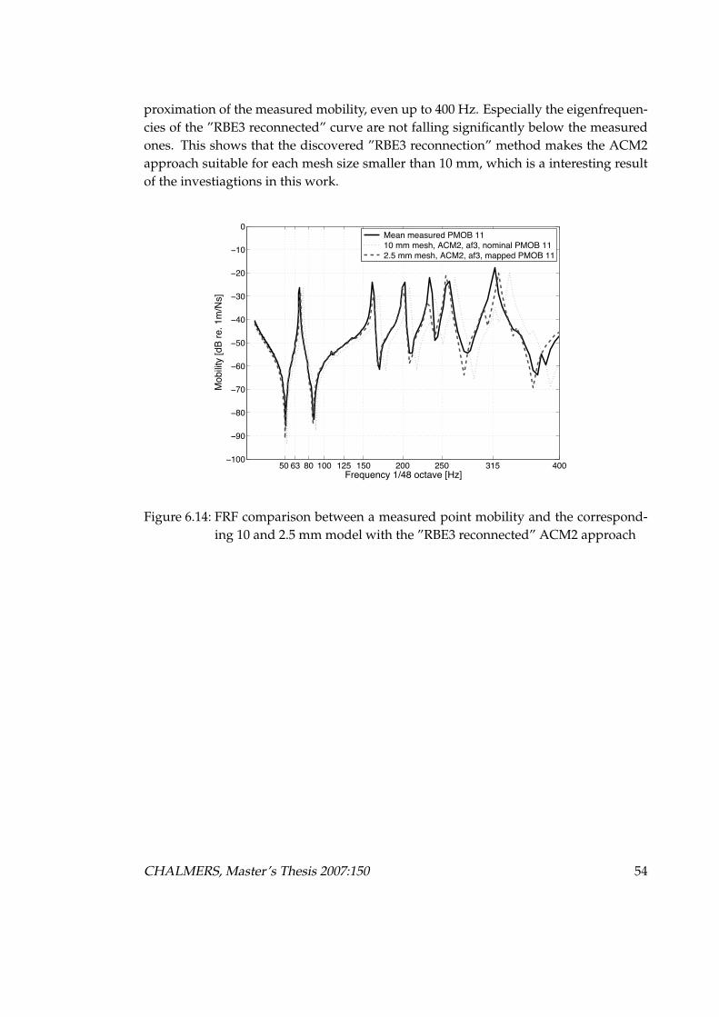
proximation of the measured mobility, even up to 400 Hz. Especially the eigenfrequen-cies of the ”RBE3 reconnected” curve are not falling significantly below the measuredones. This shows that the discovered ”RBE3 reconnection” method makes the ACM2approach suitable for each mesh size smaller than 10 mm, which is a interesting resultof the investiagtions in this work.

50 63 80 100 125 150 200 250 315 400−100

−90

−80

−70

−60

−50

−40

−30

−20

−10

0

Frequency 1/48 octave [Hz]

Mob

ility

[dB

re. 1

m/N

s]

Mean measured PMOB 11 10 mm mesh, ACM2, af3, nominal PMOB 11 2.5 mm mesh, ACM2, af3, mapped PMOB 11

Figure 6.14: FRF comparison between a measured point mobility and the correspond-ing 10 and 2.5 mm model with the ”RBE3 reconnected” ACM2 approach


7 Conclusion

In this Master’s Thesis the influence of a mapped thickness distribution and refinedpanel meshes on a benchmark FEM model has been analysed. The benchmark struc-ture was a complex three dimensional sidemember from a current Volvo car body. Theinvestigations have been done for both the single panels and the welded structure.

The results show clearly that introducing a mapped thickness distribution leads to asignificant improvement of the simulation results. For the single sidemembers and thewelded assemblies the deviation between measured and calculated eigenfrequenciescould be reduced of ca. 3% in a frequency range up to 300 Hz. So the deviation ineigefrequencies is less than 2% for the first ten modes with a mapped thickness. A ad-ditional advantage is that the improvement due to mapping works nearly unimformlyfor all modes and is a result of a better approximation of the local bending stiffnessdistribution.Also the potential of the most common spot weld modelling techniques in NVH (ACM2and CWELD) have been investigated with respect to the accuracy and robustness to re-fined panel meshes. The standard mesh size of 10 mm was refined down to 5, 2.5and 1 mm. There the results show that the CWELD model is not applicable for panelmeshes smaller than 5 mm because of its functional limitations. The investigations onthe ACM2 model shows that when keeping the patch area like for the 10 mm stan-dard mesh size no additional loss of bending stiffness is introduced by the spot weldmodel itself. The ”RBE3 reconnection” method of the origin shell corner nodes makesthe ACM2 model adaptable for all refined meshes. In general the efficiency of refin-ing the mesh size is very much dependent on the frequency range of interest. For thesidemember panels the largest improvement could be achieved with the refining stepfrom 10 down to 5 mm. There the FE-calculated eigenfrequencies up to 300 Hz could beimproved in average of approximatly 0.5%. The other two refinements didn’t changethe first ten eigenfrequencies significantly. But it’s clearly visible that with growing fre-quency the influence of mesh refinements is also increasing. So it really depends on theconcrete situation which refinement step is reasonable.

For further application of the ”RBE3 reconnected” ACM2 model it will be neces-sary to develop an ”RBE3 reconnection” code which is applicable in the standard Pre-proccessor software available in industry. Here it should be also mentioned that in

55

future there will be a demand to implement ACM2 models directly in FEM meshessmaller than 10 mm, without the use of existing connection vectors from previous mod-els. For such goals the introduction of a search radius representing the average lengthof the RBE3 connection vectors of the 10 mm standard mesh size could be a solution.


References

[01] Palmonella, M.; Friswell, M.I.; Mottershead, J.E.; Lees, A.W.: Guidlines forthe implementation of the CWELD and ACM2 spot weld models in structuraldynamics, Finite Elements in Analysis and Design 41 (193-210), 2004

[02] Fang, J.; Hoff, C.; Holman, B.; Mueller, F.; Wallerstein, D.: Weld modelingwith MSC.Nastran, Second MSC WorldWide Automotive User Conference,Dearborn,MI, USA, October 2000

[03] Heiserer, D.; Chargin, M.; Sielaff, J.: High Performance, Process Oriented,Weld Spot Approach, First MSC WorldWide Automotive User Conference,Munich, Germany, September 1999

[04] Jonscher, A.; Lewerenz, M.; Luhrs, G.: MSC.Nastran’s new spot weld elementin the CAE process, Volkswagen A.G., Wolfsburg, Germany

[05] Xu, S.; Deng, X.: An evaluation of simplified finite element models for spot-welded joints, Finite Elements in Analysis and Design 40 (1175-1194), 2004

[06] Palmonella, M.; Friswell, M.I.; Mottershead, J.E.; Lees, A.W.: Finite elementmodels of spot welds in structural dynamics: review and updating, Comput-ers and Structures 83 (648-661), 2005

[07] Donders, S.; Brughmans, M.; Hermans, L.; Tzannetakis, N: The effect of spotweld failure on dynamic vehicle performance, LMS International, Leuven,Belgium

[08] Silva, J.M.M.; Batista, F.C.; Maia, N.M.M.: Dynamic modelling of spot weldedjoints, Twelfth International Congress on Sound and Vibration, Lisbon, 2005

[09] MSC.Nastran 2003: Linear Static Analysis Users Guide, MSC.Software Cor-poration, Santa Ana, CA 92707 USA

[10] MSC.Nastran 2005: Quick Reference Guide, MSC.Software Corporation,Santa Ana, CA 92707 USA

[11] Bretl, J.L.: Connecting solid finite element models that have dissimilar mesheson the mating surfaces, Structural Dynamics Research Corporation, Milford,Ohio; USA

57

[12] Cook, R.D.: Finite Element modeling for stress analysis, University ofWisconsin-Madison, John Wiley & Sons, Inc., 1995

[13] Ewins, D.J.: Modal Testing theory, practice and application -Second Edition-,Research Studies Press LTD., Baldock, Hertfordshire, England, 2000

[14] Chen, G.: FE model validation for structural dynamics, PhD Thesis, DynamicsSection, Department of Mechanical Engineering, London, South Kensington,April 2001

[15] Petyt, M.: Introduction to finite element vibration analysis, Cambridge Uni-versity Press, Cambridge,1990

[16] Kropp, W.: Technical Acoustic 1, Department of Applied Acoustic, ChalmersUniversity of Technology,2005

[17] Friswell, M.I.; Mottershead, J.E.; Lees, A.W.: Finite element model updatingin structural dynamics, Kluwer Academic Publisher, Dodrecht, 1995

[18] Palmonella, M.: Improving finite element models of spot weld s in structuraldynamics, PhD Thesis, University of Wales Swansea, 2003

[19] MSC.Nastran 2004: Reference Manual, MSC.Software Corporation, SantaAna, CA 92707 USA

[20] MSC.Nastran Version 68: Basic Dynamic Analysis User’s Guide,MSC.Software Corporation, Santa Ana, CA 92707 USA


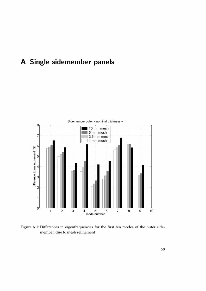
A Single sidemember panels

1 2 3 4 5 6 7 8 9 100

1

2

3

4

5

6

7

8

mode number

diffe

renc

e to

mea

sure

men

t [%

]

Sidemember outer − nominal thickness −


Figure A.1: Differences in eigenfrequencies for the first ten modes of the outer side-member, due to mesh refinement

59

0 100 200 300 400 500 600−150

−140

−130

−120

−110

−100

−90

−80

−70

−60

−50

Frequency [Hz]

Leve

l [dB

re. 1

mm

/Ns]

Sidemember inner − Influence of mapped thickness −

H11 10 mm mesh nominalH11 10 mm mesh mappedH11 Mean measured

Figure A.2: FRF comparison to show the influence of mapping - extended frequencyrange


Modelling of spot welds for NVH simulations in view of...

Documents

Transcript of Modelling of spot welds for NVH simulations in view of...