Modelling Energy Forward Curves (Borovkova).pdf

Modelling Energy Forward Curves

Svetlana Borovkova

Free University of Amsterdam (VU Amsterdam)

– Typeset by FoilTEX – 1

Energy markets

• Pre-1980s: regulated energy markets

• 1980s: deregulation of oil and natural gas industries

• 1990s: deregulation of electricity industries worldwide

• Energy is the world’s largest traded commodity class

• Crude oil is the world’s largest commodity

• Energy markets are extremely volatile (annual volatilities: Oil 40+%, NG 60+%,

Electricity 100+% −→ comp. with 15+% for equity indices)

=⇒ need for efficient risk management

• Energy prices are negatively correlated to the stock prices and indices

=⇒ perfect diversification tools

What is traded?

Physical crude oil, oil products, NG (spot markets); forward contracts (OTC);

Futures contracts on ICE, NYMEX: volumes 9-10 times higher than those in spot markets!


Futures contracts and forward curves

• Futures: standardized contracts for delivery of a commodity (e.g. crude oil) at different

time points (expiries) in the future.

• Prices for futures with different expiries (e.g., for oil, up to 72 months ahead) are

recorded daily.

• The collection of these futures prices on any particular day is called the forwardcurve.

• The set {F (t, T ), T > t} is the forward curve prevailing at date t for a given

commodity in a given location; T indicates the expiry, or maturity date (month).

• The forward curve is the fundamental tool when trading commodities, as spot prices

may be unobservable and options illiquid.


Benefits of forward curves

• Forward curves reflect market fundamentals and anticipated price trends

• Benchmark for Valuation: Deal Pricing, P & L

• Internal Consistency in the desk or the firm with other derivatives

• Mark To Market, Stop Loss, VaR

• The forward curves provide the calibration of the model parameters under the pricing

measure

• Commodity portfolios contain futures with different expiries

−→ risk exposure to movements of the entire forward curve

• Pricing of derivatives on futures and forwards requires forward curve models


The oil price in the last two decades

0 1000 2000 3000 4000 50000

10

20

30

40

50

60

70

80

$/bb

l

Trading days since 23−06−1988

WTI Crude Oil price, July 1998 − December 2006


Oil forward curves: two fundamental market statesBackwardation and Contango

Anticipated value of the future spot price is lower (B) or higher (C) than the current one.

Influenced by: current price and inventory levels, transportation and storage costs,

supply/demand, strategic and political reasons, ...

0 2 4 6 8 10 12 14 16 18 200

5

10

15

20

25

30

Expiry months (numbered from now)

$/ba

rrel

06.03.2000, backwardation market

0 2 4 6 8 10 12 14 16 18 200

2

4

6

8

10

12

14

16

Expiry months (numbered from now)

$/ba

rrel

01.12.1998, contango market


Changing face of oil market: arrival of hedge funds

Figure 1: WTI Oil forward curve, March 2006


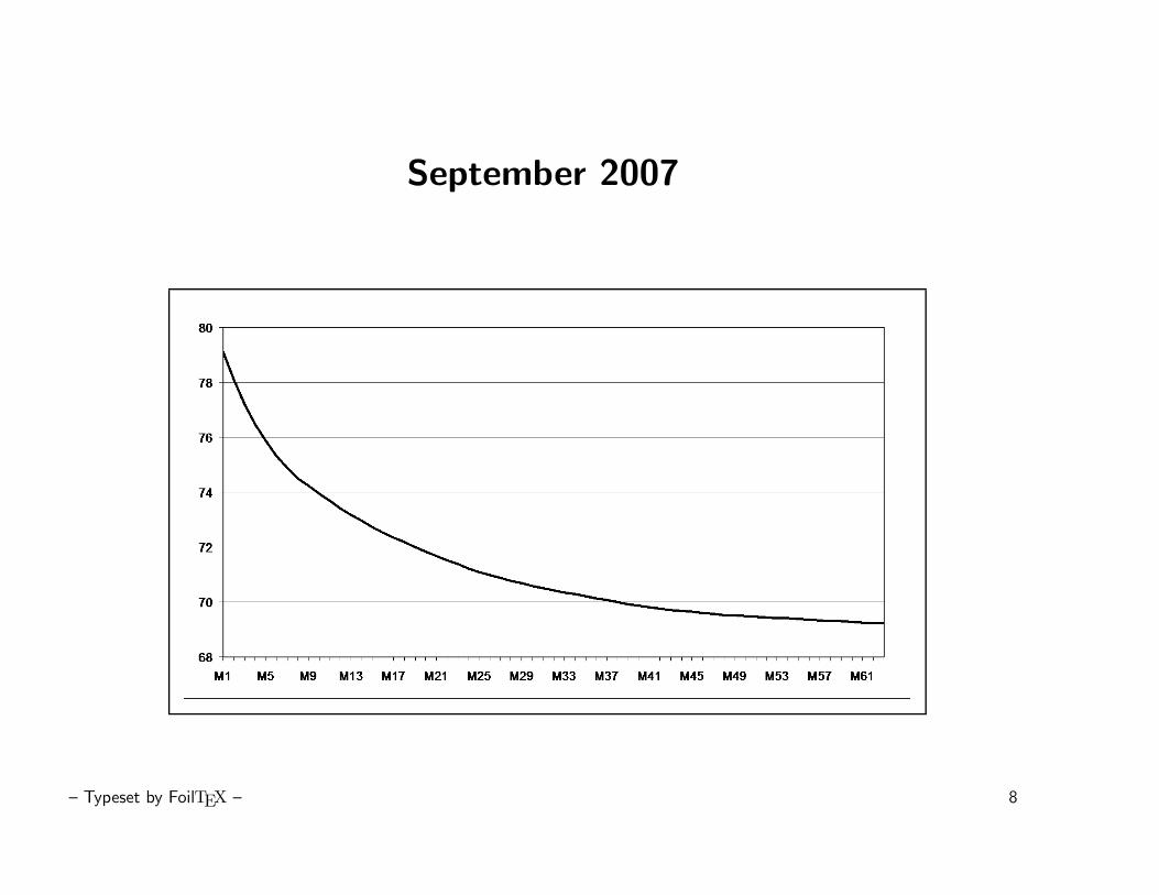
September 2007


Seasonality in commodity prices

• For oil, seasonality is not significant, since tankers are rerouted to satisfy a surge of

demand in a given region

• Energy (electricity, natural gas, spark spread) - governed by seasonal demand

• Agricultural commodities (wheat, soybean, soymeal, crush spread, coffee, cocoa) -

governed by seasonal supply

• Seasonality in energy or agricultural spot prices:

well-understood and easily modelled (e.g. mean-reversion with seasonally varying mean,

seasonal component + autoregression)

• Seasonality in forward curves:

much less studied; no ”explicit” models


Example of Natural Gas forward curve:

0 10 20 30 40 50 60 706.5

7

7.5

8

8.5

9

9.5

Months to maturity

Ste

rling

pen

ce p

er th

erm

Natural gas forward curve, March 7, 2007


Futures vs. spot prices: Theory of Storage

Cost-of-carry relationship (no-arbitrage arguments):

F (t, T ) = S(t)e[r(t)+w(t)](T−t)

(∗)

r(t): spot interest rate, w(t): marginal storage costs per $ of spot, per time unit.

In practice (∗) almost never holds (e.g. backwardation or hump-shaped forward curves):

strategic importance (oil); limited or non-storability (agricultural, electricity)

Convenience of having physical commodity as opposite to futures contract

−→ concept of convenience yield y(t):

F (t, T ) = S(t)e[r(t)−y(t)](T−t)

- premium (as perceived on the day t) earned by an owner of physical commodity asopposite to an owner of the futures contract with maturity T .


Convenience yield

• Often considered net marginal storage costs: y(t) = y(t) − w(t).

• Convenience yield proportional to the spot price y(S): Brennan & Schwartz (1985).

• Stochastic convenience yield y(t) = y(t, ω): Gibson & Schwartz (1990), Schwartz

(1997).

• Dependence on t: ”premium” to owner of physical commodity changes with inventories

(stocks) and hence, with agents’ preference for physical rather than paper.

• At a fixed date t, a single value of the process (y(t))t for all maturities is not

compatible with the hump-shaped forward curve observed in 2006 in the oil market (and

other commodity markets), or with seasonal features of the forward curve.


Theory of Storage revisited

• One possible modelling answer is to introduce a term structure y(t, T ) of convenience

yields at date t, deterministic in the maturity argument T and stochastic in t

(Borovkova & Geman, 2006, 2007)

• This approach is certainly beneficial in the case of seasonal commodities such as

natural gas where, assuming today = January 2008, y(t, T ) should be different for T =

September 2008 or T = December 2008.

• Dependence of convenience yield on maturity T (y(t, T )): to emphasize seasonality of

F (t, T ) in

F (t, T ) = S(t)e[r(t)−y(t,T )](T−t)

e.g. futures expiring at ”desirable” season (e.g. NG futures expiring in December)

Emphasizes the time-spread option feature of convenience.


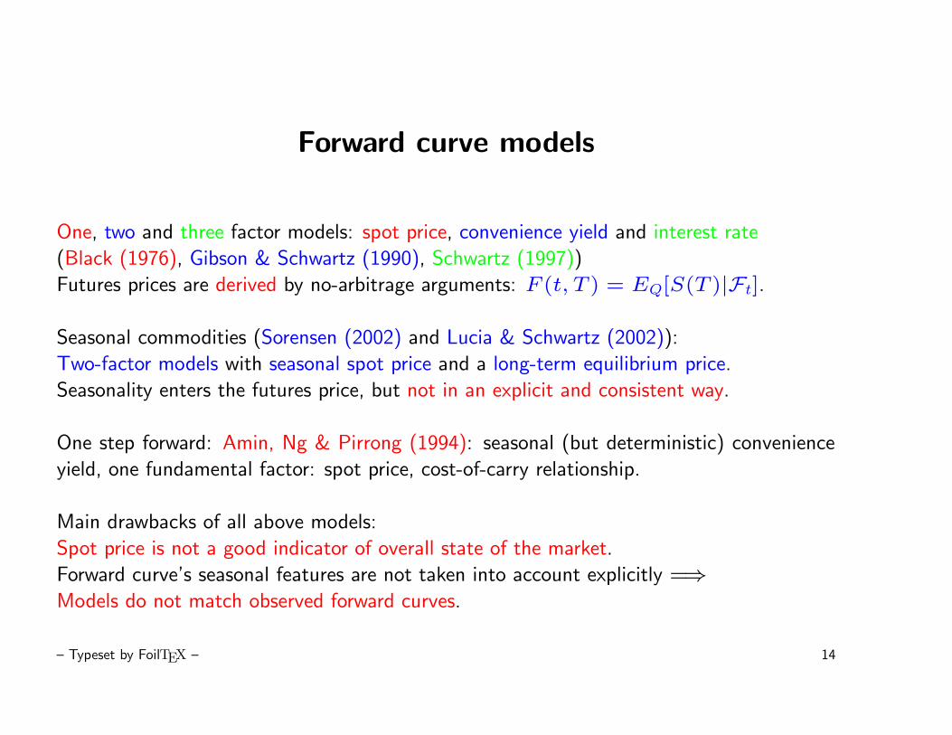
Forward curve models

One, two and three factor models: spot price, convenience yield and interest rate

(Black (1976), Gibson & Schwartz (1990), Schwartz (1997))

Futures prices are derived by no-arbitrage arguments: F (t, T ) = EQ[S(T )|Ft].

Seasonal commodities (Sorensen (2002) and Lucia & Schwartz (2002)):

Two-factor models with seasonal spot price and a long-term equilibrium price.

Seasonality enters the futures price, but not in an explicit and consistent way.

One step forward: Amin, Ng & Pirrong (1994): seasonal (but deterministic) convenience

yield, one fundamental factor: spot price, cost-of-carry relationship.

Main drawbacks of all above models:

Spot price is not a good indicator of overall state of the market.

Forward curve’s seasonal features are not taken into account explicitly =⇒Models do not match observed forward curves.


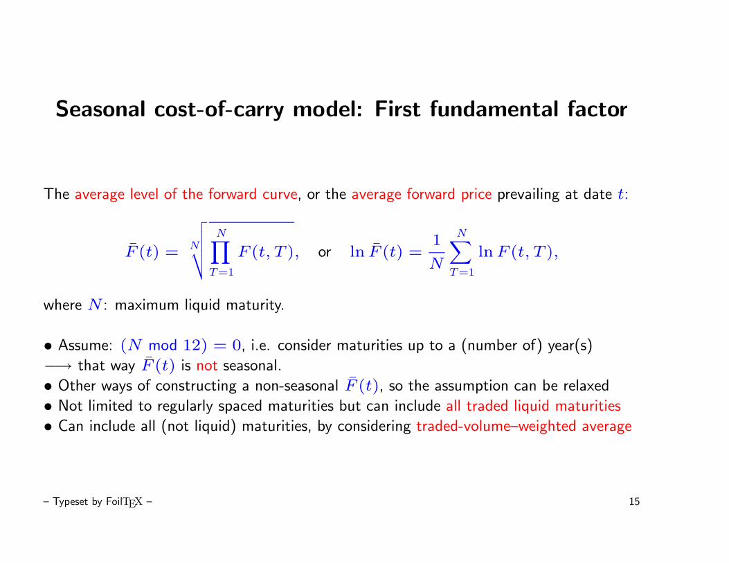
Seasonal cost-of-carry model: First fundamental factor

The average level of the forward curve, or the average forward price prevailing at date t:

F (t) = N

√√√√ N∏T=1

F (t, T ), or ln F (t) =1

N

N∑T=1

ln F (t, T ),

where N : maximum liquid maturity.

• Assume: (N mod 12) = 0, i.e. consider maturities up to a (number of) year(s)

−→ that way F (t) is not seasonal.

• Other ways of constructing a non-seasonal F (t), so the assumption can be relaxed

• Not limited to regularly spaced maturities but can include all traded liquid maturities

• Can include all (not liquid) maturities, by considering traded-volume–weighted average


Seasonal cost-of-carry model: Seasonal premium

The seasonal premium (s(M))M=1,...,12 is the collection of long-term–averagepremia (expressed in %) on futures expiring in the calendar month M (M = 1, ..., 12)

with respect to the average forward price F (t).

• Assume (s(1), ..., s(12)) is the deterministic collection of 12 parameters;

• Require that∑ 12

M=1 s(M) = 0;

• Seasonal premium is an absolute quantity and not a rate: premium on futures expiring

in July is the same whether today is June or December. Premium on July 2008 futures is

the same as on July 2009 futures.

• Can be defined as a continuous-time periodic function (e.g. trigonometric); however less

appropriate for monthly expiries.


Seasonal cost-of-carry model: The model

For any maturity T , we write

F (t, T ) = F (t)e[s(T )−γ(t,T )(T−t)]

, (∗)

where γ(t, T ), defined by the relationship (∗), is called the stochastic convenience yieldnet of seasonal premium, for maturity T , as perceived on the day t.

Seasonal (monthly) premium (or discount): in s(T )

Stochastic factors influencing forward prices: in γ(t, T )

The relationship (∗) involves only forward prices, hence no interest rates.


Features of the model

Relationship to classic convenience yield models:

γ(t, T ) − s(T )

T − t= y(t, T ) − 1

N

N∑K=1

y(t, K)

−→ γ(t, T ) can be interpreted as the relative convenience yield net of the (scaled)seasonal premium.

• Convenience yield γ can be used for non-storable commodities (e.g. electricity),

since spot price plays no role

• If γ(t, T ) ≡ 0 −→ one-factor model driven by F (t) and deterministic s(T )

• If s(T ) = 0 ∀T , then no deterministic seasonality (e.g. oil) and γ(t, T ) is the

”relative convenience yield” −→ two-factor model similar to Gibson & Schwartz (1990)

but with F (t) instead of the spot price.


Dynamics of fundamental factors and futures prices

F (t) is not seasonal by construction

−→ can be modelled as a mean-reversion with constant mean, or GBM.

γ(t, T ) is essentially zero (on average), since all systematic deviations are in s(T )

−→ can be modelled as a mean-reversion with mean zero.

All stochastic convenience yields (γT (t))T=1,...,N are driven by the same Brownian

motion, independent of the BM driving the average forward price.

Seasonal cost-of-carry + dynamics of (F (t), γT (t)) = dynamics of (F (t, T ))T .

Resulting futures prices F (t, T ) are log-normal with instantaneous proportional variance

ξ2(t, T ) = σ

2+ (η

T(T − t))

2 − 2σρηT(T − t)


Model estimation

Historical data of daily forward curves (F (t, 1), ..., F (t, 12))t=1,...,n.

Estimate

• the daily average forward price by ln F (t) = 112

∑ 12M=1 ln F (t, M);

• the seasonal premia (s(M))M , according to the definition, by

s(M) =1

n

n∑t=1

[ln F (t, M) − ln F (t)], M = 1, ..., 12,

• the stochastic convenience yield by

γ(t, T ) = (− ln(F (t, T )/F (t)) + s(T ))/((T − t)).

More than 12 maturities: easily incorporated, but if fewer than 12 maturities, the

unbiased estimate for F (t) is not available

−→ a more complicated estimation procedure.


Seasonal premium for Natural Gas futures

1 2 3 4 5 6 7 8 9 10 11 12−0.2

−0.15

−0.1

−0.05

0

0.05

0.1

0.15

0.2

0.25

0.3

Calendar month

Seas

onal

pre

miu

m in

%

Seasonal premium for NG futures


Seasonal premium for electricity futures

1 2 3 4 5 6 7 8 9 10 11 12−0.2

−0.15

−0.1

−0.05

0

0.05

0.1

0.15

Calendar month

%

Seasonal forward premium, Electricity futures


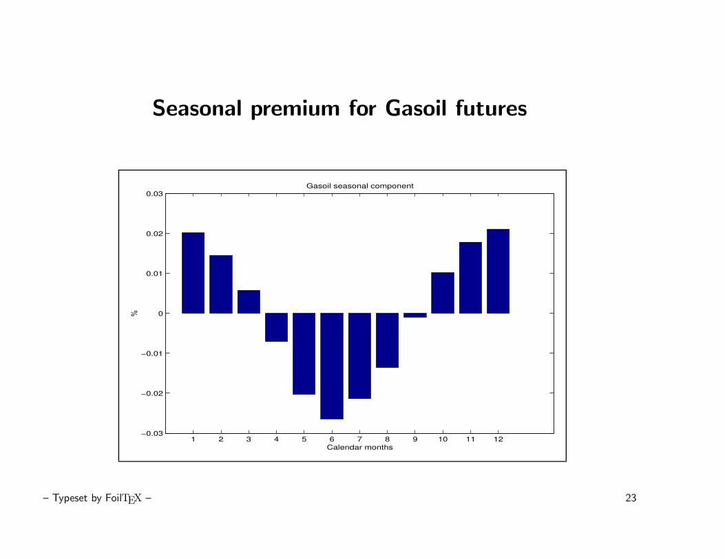
Seasonal premium for Gasoil futures

1 2 3 4 5 6 7 8 9 10 11 12−0.03

−0.02

−0.01

0

0.01

0.02

0.03

Calendar months

%

Gasoil seasonal component


Seasonal premium for spark spread

1 2 3 4 5 6 7 8 9 10 11 12−0.6

−0.5

−0.4

−0.3

−0.2

−0.1

0

0.1

0.2

0.3

0.4

Calendar month

%

Seasonal forward premium, Spark spread


Term structure of stochastic forward premium volatilities, Gasoil futures

1 2 3 4 5 6 7 8 9 10 11 120

0.02

0.04

0.06

0.08

0.1

0.12

0.14

Maturity

%

Volatility of (Gamma(t,T)), T=1,...,12


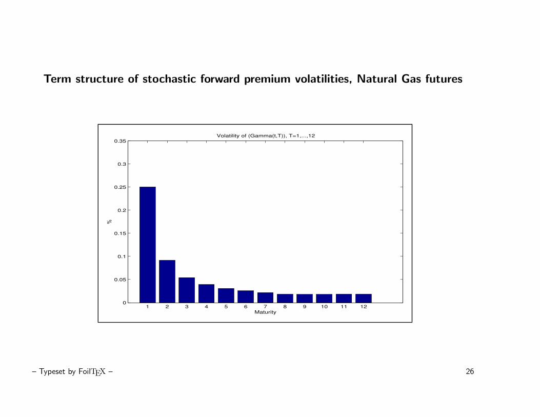
Term structure of stochastic forward premium volatilities, Natural Gas futures

1 2 3 4 5 6 7 8 9 10 11 120

0.05

0.1

0.15

0.2

0.25

0.3

0.35

Maturity

%

Volatility of (Gamma(t,T)), T=1,...,12


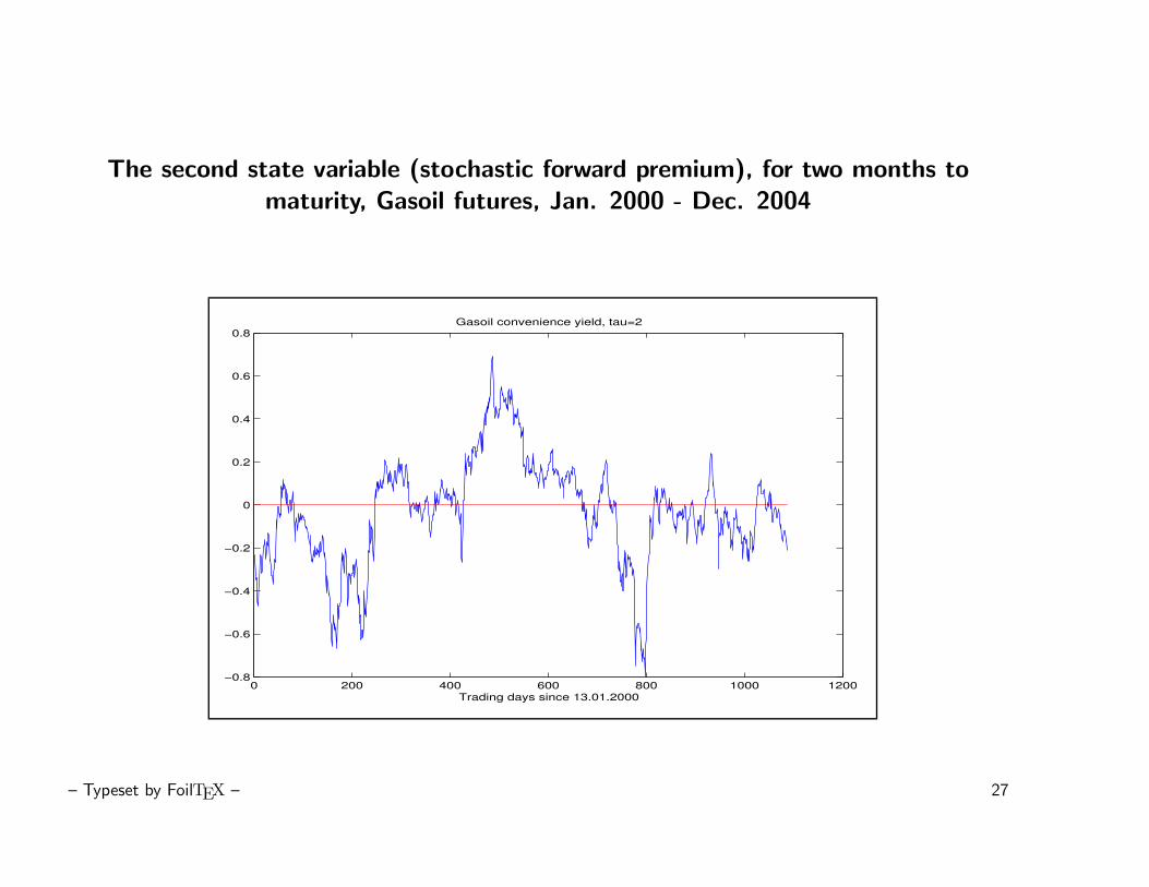
The second state variable (stochastic forward premium), for two months tomaturity, Gasoil futures, Jan. 2000 - Dec. 2004

0 200 400 600 800 1000 1200−0.8

−0.6

−0.4

−0.2

0

0.2

0.4

0.6

0.8Gasoil convenience yield, tau=2

Trading days since 13.01.2000


Properties of the convenience yield

• All observed series (γ(t, T ))t can be modelled by low-order autoregression(order 2 - 5) −→ autoregressive structure can be exploited for- forecasting the stochastic convenience yield- forecasting market conditions- devising market indicators- generating profitable trading strategies• Convenience yield can be regressed on economic fundamentals andexogenous market variables, e.g. supply/demand, volatility, ...

Mean-reversion parameters (T = 2):electricity gas gasoil oil

aT : 0.07 0.09 0.02 0.01ηT : 0.16 0.10 0.05 0.04


Relationship of γ(t, T ) to market indicators and economicfundamentals

Theory of storage + empirical considerations−→ conjectures about the convenience yield:

I. It is positively correlated to the overall price level (given by eitherspot price or average forward price)

II. It is negatively correlated to inventories

III. It is positively correlated to spot price’s volatility

IV. It is negatively correlated to the correlation between spot and futuresprices.


Conjecture I: true, especially for higher maturities: Gasoil

5 5.1 5.2 5.3 5.4 5.5 5.6 5.7 5.8−0.05

0

0.05

0.1

0.15

0.2

Log Fbar

Stoc

hast

ic co

nven

ienc

e yie

ld, T

=12

Stochastic convenience yield, T=12, vs average forward price


Conjecture I: true, especially for higher maturities: NG

5 10 15 20 25 30 35−0.5

−0.4

−0.3

−0.2

−0.1

0

0.1

0.2

0.3

0.4

NG M futures price, pence/term

Stoc

hast

ic 6−

mon

th c

onve

nien

ce y

ield

Stochastic conv. yield vs NG M price: blue: 01.97−03.00, red: 03.00−02.02


Extracting the seasonal component

Seasonal component is ”known” monthly premium −→ extract it from aforward curve. If seasonality was the only determining factor, then what isleft should always be flat, but it is not!=⇒ situations similar to backwardation/contango arise:

1 2 3 4 5 6 7 8 9−1.5

−1

−0.5

0

0.5

1

Months to expiry

Ste

rling

/MW

h

De−seasoned electricity forward curve, 27.06.01

1 2 3 4 5 6 7 8 9−1

−0.5

0

0.5

1

1.5

2

2.5

Months to expiry

Ste

rling

/MW

h

De−seasoned electricity forward curve, 15.12.01


Principal Component Analysis of the forward curveCase I: interest rates and non-seasonal commodities (oil)

A forward curve of almost any shape can be constructed by combining three simple shapes:

Level, Slope, Curvature

−→ Principal Components of (F(t))t∈N = (F1(t), F2(t), ..., FN(t))t∈N

0 2 4 6 8 10 12 14 16 18 200

0.05

0.1

0.15

0.2

0.25

0.3

0.35

Expiry0 2 4 6 8 10 12 14 16 18 20

−0.5

−0.4

−0.3

−0.2

−0.1

0

0.1

0.2

0.3

0.4

Expiry0 2 4 6 8 10 12 14 16 18 20

−0.3

−0.2

−0.1

0

0.1

0.2

0.3

0.4

0.5

Expiry

First three principal components explain approx. 99% (!) of the forward curve’s variability.

(Litterman & Scheinkmann ’91 for US government bonds, Cortazar & Schwartz ’94 for

copper)


Principal Components of daily returns

0 2 4 6 8 10 12 14 16 18 200

0.05

0.1

0.15

0.2

0.25

0.3

0.35

Expiry0 2 4 6 8 10 12 14 16 18 20

−0.5

−0.4

−0.3

−0.2

−0.1

0

0.1

0.2

0.3

0.4

Expiry0 2 4 6 8 10 12 14 16 18 20

−0.4

−0.2

0

0.2

0.4

0.6

0.8

1

Expiry

These first three principal components have clear economic interpretation,explain 95% of the total variability, can be treated as the main risk factorsgoverning the futures prices’ evolution.


Applications of PCA

I. Forecasting market transitions (between backwardation and contango):

• The second principal component reflects the slope of the forward curve

• Values close to 0 indicate a flat forward curve (and hence, possible transition)

• Due to smooth time-series-like structure, it can be used to construct an indicator which

anticipates possible transitions

Borovkova, EPRM magazine (June 2003).

II. Portfolio risk management and VaR estimation

• First few principal components (of returns) reflect main risk factors

=⇒ the number or risk factors is greatly reduced

• The distribution of portfolio returns can be approximated via the distribution of the main

risk factors

• In a portfolio context, these risk factors can be hedged


Principal Component Indicator

”Raw” version: projection of the daily forward curve on the second PC

I(t) =

N∑k=1

PCL(2)k Fk(t),

where PCL(2)k (k = 1, ..., N) are second principal component loadings of the futures

prices series.

MA-smoothed version:

IMA

(t) =1

M

M−1∑i=0

I(t − i).

Choice of M : take a fast and slow moving average.


Application of the PC indicator to Brent oil futures

Generate a ”signal of change” when the indicator enters some ε-neighborhood of zero:

0 100 200 300 400 500 600 700 800 900 1000−1

−0.5

0

0.5

1

1.5

2

2.5

3

Days

$/bb

l

0 100 200 300 400 500 600 700 800 900 1000−15

−10

−5

0

5

10

15

Days

$

PC test statistics with intermonth differences

ε-neighborhood determined via the distribution of the indicator (under the null-hypothesis

of no change), approximated by either Monte-Carlo or bootstrap distribution.


PCA for seasonal commodities (electricity, NG)

Apply PCA to deseasonalized forward curves F (t, T ) exp(−s(T )))Second and third PCs for de-seasoned FC (first PC = level) still reflect theslope and curvature:

1 2 3 4 5 6 7 8 9−0.4

−0.2

0

0.2

0.4

0.6

0.8

1

Months to expiry

PC

1 lo

adin

gs

First principal component loadings, de−centered, de−seasoned electricity FC

1 2 3 4 5 6 7 8 9−0.8

−0.6

−0.4

−0.2

0

0.2

0.4

0.6

Months to expiry

PC

2 lo

adin

gs

Second principal component loadings, de−centered, de−seasoned electricity FC


Applications of PCA: trading

• For deseasonalized forward curves, situations analogous tobackwardation/contango markets arise, in terms of deviations from the”typical” seasonal forward curve.

• High absolute values of the second PC indicates whether futures withshorter (longer) expiries are overpriced w.r.t. ”typical” seasonal premium

• Again, use PC indicator: the projection of the daily deseasonalizedforward curve on the second PC.


Principal Component Indicator for electricity FC

A value of the indicator far from zero signals significant deviation fromthe ”expected” seasonal forward curve pattern:

0 50 100 150 200 250−4

−3

−2

−1

0

1

2

3

Days

PC

1 sc

ores

First principal component scores, de−centered, de−seasoned electricity FC

Can construct profitable trading strategies based on the indicator.(Borovkova & Geman (SNDE 2006)).


Conclusions

• Extracting deterministic seasonality from forward curves allows tostudy features obscured by dominant seasonal effects (PCA, cost-of-carry,traditional term structure models)

• Average forward price is a robust identifier of the overall price level,more so than the spot price, although now need to take into accountsloping forward curves

• Stochastic convenience yield is a quantity indicative of market stateand economic indicators; it can be exploited to construct market indicatorsand generate profitable trading strategies


Perspective research directions

• Backwardation/contango-like profile in seasonal forward curves

• Applications of the model to the derivatives pricing

• Relating the stochastic convenience yield to economic and other exogenousvariables such as stocks (supply), extreme weather conditions (demand), ... .

• Modelling the entire term structure of convenience yields, with a numberof sources of uncertainty and volatility functions

• Seasonal term structure of futures prices’ volatilities

• Applications of the model to agricultural commodities


Modelling Energy Forward Curves (Borovkova).pdf

Documents

Transcript of Modelling Energy Forward Curves (Borovkova).pdf