
Modelling and Simulation of Rigid and Flexible Multibody ... · PDF fileMultibody Systems in...
58
Multibody Systems in Modelica >03.03.2008 Slide 1 Modelling and Simulation of Rigid and Flexible Multibody Systems in Modelica Tutorial at the Modelica‘2011 Conference Dresden, March 20 th , 2011 Dr.-Ing. Andreas Heckmann, German Aerospace Center (DLR) Institute of Robotics and Mechatronics
Transcript of Modelling and Simulation of Rigid and Flexible Multibody ... · PDF fileMultibody Systems in...
Multibody Systems in Modelica >03.03.2008
Slide 1
Modelling and Simulation of Rigid and Flexible Multibody Systems in Modelica
Tutorial at the Modelica‘2011 Conference Dresden, March 20th, 2011 Dr.-Ing. Andreas Heckmann, German Aerospace Center (DLR) Institute of Robotics and Mechatronics
Multibody Systems in Modelica > 20.03.2011
slide 2
Contents
Modelica Multibody BasicsExercise 1: Control of an inverse pendulumModelica Multibody AdvancedExercise 2: The Flying Gull IFlexibleBodies Library: BeamsExercise 3: The Flying Gull IIExercise 4: A classic PitfallExercise 5: Unbalanced ShaftFlexibleBodies Library: General bodies based on finite element dataExercise 6: The Flying Gull IIIFE-PreprocessingFlexibleBodies Library extensions at this conference

Multibody Systems in Modelica > 20.03.2011
slide 3
Modelica Multibody Basics: Orientation
1r12
R12
l ( )1
2
e1z e1y
e1x
e2x
e2ye2z
h
Coordinate systems and their orientation
Orientation object R12
describes orientation of coordinate system 2 wrt.1holds
may be computed using rotation angles or quaternionsMultibody Lib. contains over 30 functions to operate on orientation objects

Multibody Systems in Modelica > 20.03.2011
slide 4
Modelica Multibody Basics: Connectors IConnectors: the interface to connect components
Position is resolved in world frameForces and torques are resolved in local frame
0r0a
R0aa
0
af
a
world framecut plane
frame a
flow !
non-flow !

Multibody Systems in Modelica > 20.03.2011
slide 5
Modelica Multibody Basics: Connectors IIConnectors: how they work
Modelica‘s general connections rulesnon-flow variables are set to be equal, i.e. frames coincide
since they represent „some kind of potential“flow variables sum to zero (Kirchhoff‘s current law)
since they represent time derivatives of preserved quantitiesare consequently set to zero if connector is not connected to anything
see Modelica.UsersGuide.Connectors for a comparison of connectors in various domains

Multibody Systems in Modelica > 20.03.2011
slide 6
Modelica Multibody Basics: Components IKinematics:
Component equations provide relations between connector variables on position levelMultiBody.Parts.FixedTranslation i.e. fixed translation of frame_b with respect to frame_aTool (e.g. Dymola) differentiates these equations twice for dynamics
fixedTranslation
r={.1,3,1.5}
a b

Multibody Systems in Modelica > 20.03.2011
slide 7
Modelica Multibody Basics: Components IIDynamics
Newton-Euler equationsMultiBody.Parts.Body r_CM
body
center of mass
frame_a

Multibody Systems in Modelica > 20.03.2011
slide 8
Modelica Multibody Basics: Elementary Components IModelica.Mechanics.MultiBody.World
defines inertial frame, gravity, animation defaults
Modelica.Mechanics.MultiBody.Forcesdifferent resolution propertiesinterface to Real input functions and 1D mechanicsseveral spring/damper configurations
world
x
y
world
worldForceAndTorque
a b
resolve
torque
a b
springDamperParallel
c,d=c,0a b
lineForceWithMass

Multibody Systems in Modelica > 20.03.2011
slide 9
Modelica Multibody Basics: Elementary Components IIModelica.Mechanics.MultiBody.Joints
define specific degree of freedomcapability to set-up initial configurationinterface to/for 1D mechanics and rheonom motione.g.:
Modelica.Mechanics.MultiBody.PartsFixed, FixedTranslation and FixedRotation
fixed
r={0,0,0}
fixedTranslation
r={0,0,0}
a b
fixedRotation
r={0,0,0}
a
b
ba
prismaticn={1,0,0}
a b
n={0,0,1}revolute
a buniversal
a bspherical

Multibody Systems in Modelica > 20.03.2011
slide 10
Modelica Multibody Basics: Elementary Components IIIModelica.Mechanics.MultiBody.Parts
Rigid bodies with predefined geometric shapes
Modelica.Mechanics.Multibody.Sensorsfor control and validation purposes
Modelica.Blocks.Sources + Modelica.Blocks.Math
m=1
bodybodyBox
r={0.1,0,0}
ba
bodyCylinder
r={0.1,0,0}
a b
cutForceAndTorque
a b
resolve
a b
distancerelativeSensor
a b
resolve
sine
freqHz=1
ramp
duration=2 k=1
gain
-
feedback

Multibody Systems in Modelica > 20.03.2011
slide 11
Modelica Multibody Basics: Analysis MethodsModel checkExperiment setup, translation and time simulation

Multibody Systems in Modelica > 20.03.2011
slide 12
Modelica Multibody Basics: Analysis MethodsModel checkExperiment setup, translation and time simulationEigenvalue analysis
Menu: FileLibrariesLinearSystems

Multibody Systems in Modelica > 20.03.2011
slide 13
Example 1: Control of an inverse pendulum IInitial model
Box: 0.5 x 0.25 x 0.25 mactuatedRevolute: phi.start =95°, fixed=trueperform time simulation and eigenvalue analysis
world
x
y
bodyBox
r={.5,0,0}
ba
bodyCylinder
r={1,0,0}
a b
fixedTranslation
r={.25,0.125,0}
a ba b
n={0,0,1}Revolute
ba
n={1,0,0}
prismatic

Multibody Systems in Modelica > 20.03.2011
slide 14
Exercise 1: Control of an inverse Pendulum IIstate space control
Multibody Systems in Modelica > 20.03.2011
slide 15
Contents
Modelica Multibody BasicsExercise 1: Control of an inverse pendulumModelica Multibody AdvancedExercise 2: The Flying Gull IFlexibleBodies Library: BeamsExercise 3: The Flying Gull IIExercise 4: A classic PitfallExercise 5: Unbalanced ShaftFlexibleBodies Library: General bodies based on finite element dataExercise 6: The Flying Gull IIIFE-PreprocessingFlexibleBodies Library extensions at this conference

Multibody Systems in Modelica > 20.03.2011
slide 16
Joints AND bodies have potential statesnumber of joints is independent from number of bodiesan assignment of joints to bodies is not mandatoryforce elements may be connected to each othere.g.:
here: body coordinates: position, quaternions and their derivatives are used as states
Modelica Multibody Advanced: State selection I
world
x
y m=0.8
body1
bar1
r={0.3,0,0}a b a b
spring1
c=20
bar2
r={0,0,0.3}
a b
a b
spring2
c=40
a b
spring3
c=20

Multibody Systems in Modelica > 20.03.2011
slide 17
relative joint coordinates are used as states if possibledefault: stateSelect = StateSelect.prefere.g. Multibody.Joints.Prismatic
Advanced user may influence state selection directly
Modelica Multibody Advanced: State selection II
sframe_a frame_b

Multibody Systems in Modelica > 20.03.2011
slide 18
Modelica Multibody Advanced: Loops IStandard case
no specific action by the user is requiredevery connector is one node in the virtual connection graphroots of the virtual connection graph are found, e.g. world.frame_bloops are virtually broken
root
potential root
node
nonbreakable branch (Connections.branch)breakable branch (connect) removed breakable branch to get tree
root root
selected (potential) root
Multibody Systems in Modelica > 20.03.2011
slide 19
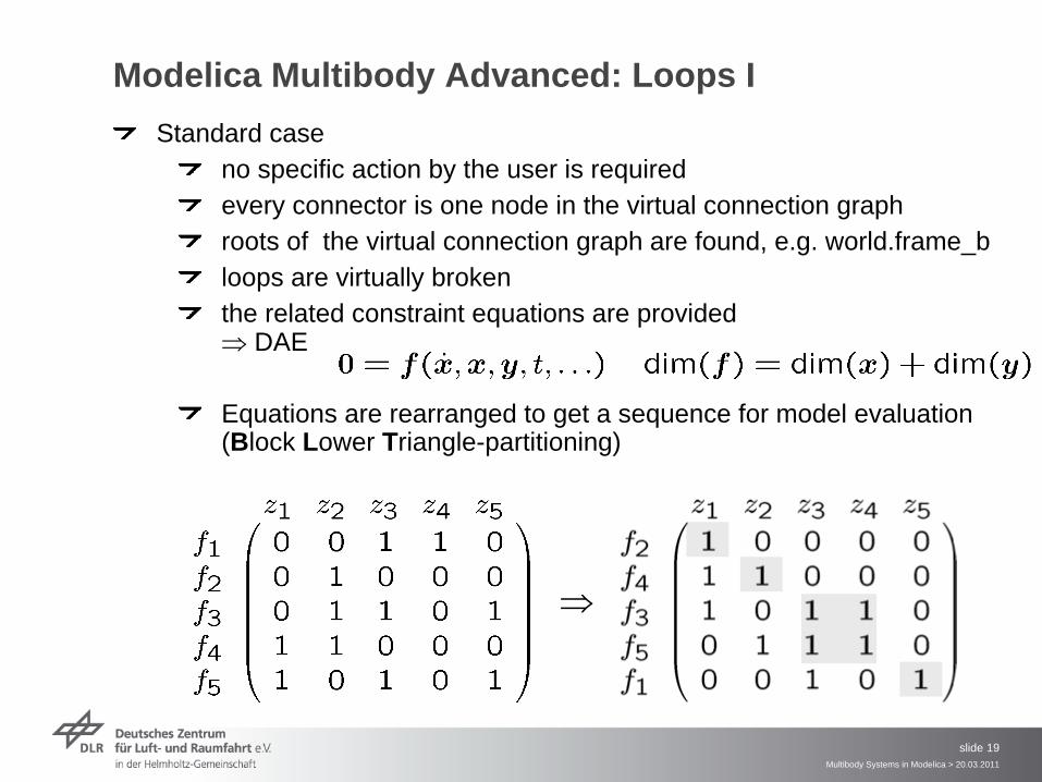
Modelica Multibody Advanced: Loops IStandard case
no specific action by the user is requiredevery connector is one node in the virtual connection graphroots of the virtual connection graph are found, e.g. world.frame_bloops are virtually brokenthe related constraint equations are provided DAE
Equations are rearranged to get a sequence for model evaluation (Block Lower Triangle-partitioning)

Multibody Systems in Modelica > 20.03.2011
slide 20
Modelica Multibody Advanced: Loops IStandard case
no specific action by the user is requiredevery connector is one node in the virtual connection graphroots of the virtual connection graph are found, e.g. world.frame_bloops are virtually brokenthe related constraint equations are provided DAE
Equations are rearranged to get a sequence for model evaluation (Block Lower Triangle-partitioning)Equations to be differentiated are determined (Pantelides algorithm)superflous potential states are deselected dynamically (dummy derivative method) ODE:

Multibody Systems in Modelica > 20.03.2011
slide 21
Modelica Multibody Advanced: Loops IIreview Translation Log in order to streamline simulation performance with model adjustments

Multibody Systems in Modelica > 20.03.2011
slide 22
Modelica Multibody Advanced: Loops IIIPlanar loops
error message

Multibody Systems in Modelica > 20.03.2011
slide 23
Modelica Multibody Advanced: Loops IVUse of aggregrated joint objects
to profit from analytical loop handling according to the „characteristic pair of joints“ method by the group of Prof. Hiller
Piston
r={0,-0.1,0}
ab
Rod2
r={0,0.2,0}ba
a b
n={1,0,0}Bearingworld
x
y
Inertia
J=0.1
Crank4
.b
a
Crank3
r={0.1,0,0}a b
Crank1
r={0.1,0,0}a b
b
a
Mid
r={0.05,0,0}a b
cylPosition
r={0.15,0.55,0}
a b
gasForce...a b
ab
jointRRP
ib ia
n_a={1,0,0}
im
Crank2

Multibody Systems in Modelica > 20.03.2011
slide 24
Modelica Multibody Advanced: InitialisationInitialisation default:
every state is assumed to be arbitrary unless otherwise providedNewton solver starts with guess value zero in order to find consistent initial states unless otherwise provided
If initialisation failsdetermine, i.e. fix, characteristic variables/states in order to influence the system of equations to solveprovide „good“ guesses for initial statesbe aware of singular positions, e.g. piston at bottom dead centerkeep initialisation system consistent
Multibody Systems in Modelica > 20.03.2011
slide 25
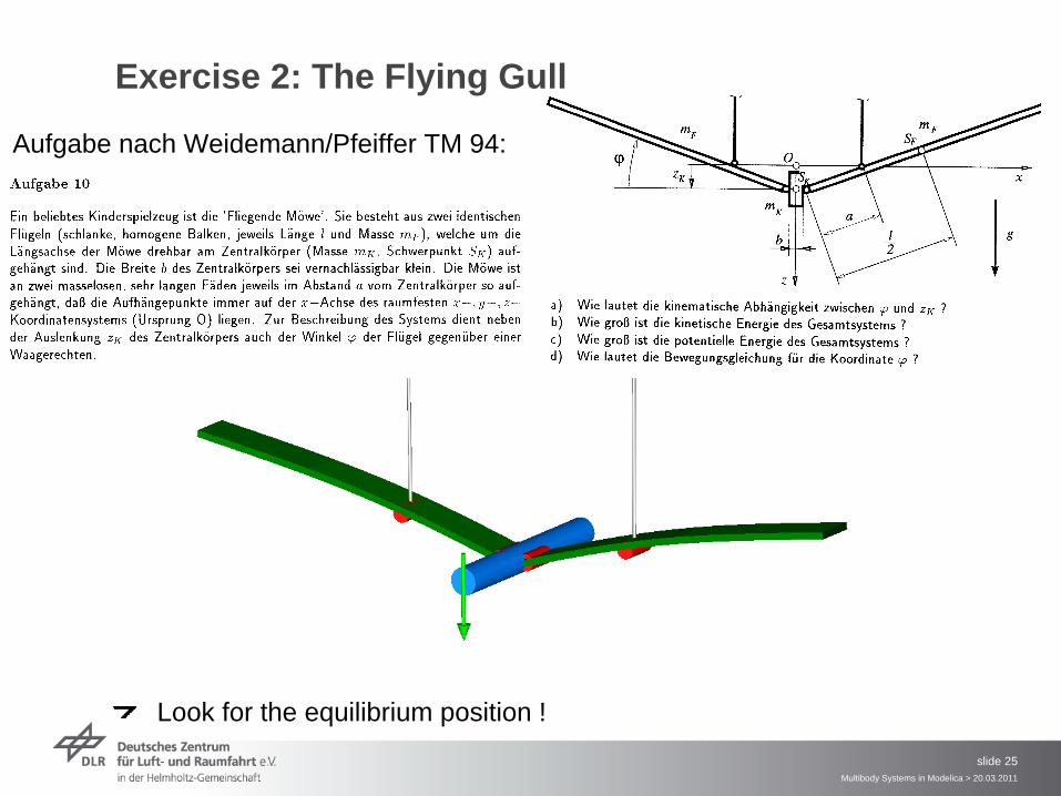
Exercise 2: The Flying Gull
Look for the equilibrium position !
Aufgabe nach Weidemann/Pfeiffer TM 94:

Multibody Systems in Modelica > 20.03.2011
slide 26
Exercise 2: The Flying Gull I
PlanarRotationSequence {-90°,0,90°}
PlanarRotationSequence {90°,0,90°}
width=0.12 m height=0.005 m =1000 kg/m3
Ø=0.08m, =200 kg/m3
width=0.12 m height=0.005 m =1000 kg/m3

Multibody Systems in Modelica > 20.03.2011
slide 27
Contents
Modelica Multibody BasicsExercise 1: Control of an inverse pendulumModelica Multibody AdvancedExercise 2: The Flying Gull IFlexibleBodies Library: BeamsExercise 3: The Flying Gull IIExercise 4: A classic PitfallExercise 5: Unbalanced ShaftFlexibleBodies Library: General bodies based on finite element dataExercise 6: The Flying Gull IIIFE-PreprocessingFlexibleBodies Library extensions at this conference

Multibody Systems in Modelica > 20.03.2011
slide 28
The name of the game : 2 types of modelling elements
Semi-analytical description implemented in ModelicaModelica generates SIDAnimation uses analytical description
FEM-based body description (Abaqus-SID- interface, SIMPACK-FEMBS)Modelica reads externally generated SID fileModelica reads externally generated ani- mation data (wavefront) file
What do they have in common ?Floating frame of reference approach
Structure of equations of motionData structure, so called SID(Standard-Input-Data: Wallrapp ’94)
In what do they differ ?

Multibody Systems in Modelica > 20.03.2011
slide 29
Theory: the equations of motion
principle of virtual power
equations of motion: here
SID structure: definition of file format to file volume integrals
the generalized Newton-Euler-equations of motion of an unconstrained deformable body
Multibody Systems in Modelica > 20.03.2011
slide 30
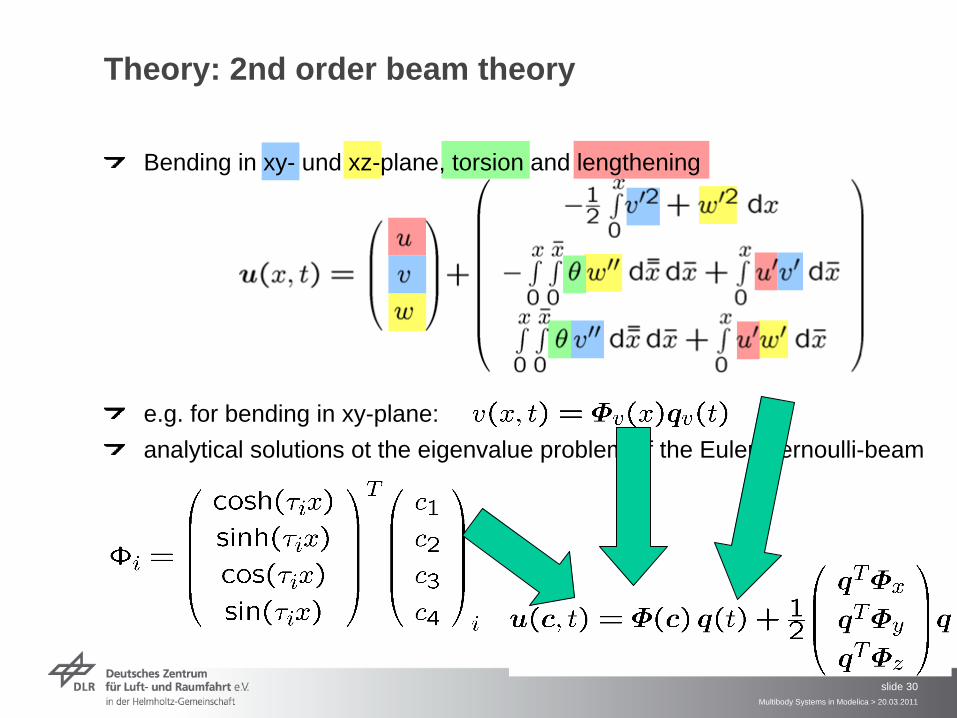
Theory: 2nd order beam theory
Bending in xy- und xz-plane, torsion and lengthening
e.g. for bending in xy-plane: analytical solutions ot the eigenvalue problem of the Euler-Bernoulli-beam
Multibody Systems in Modelica > 20.03.2011
slide 31
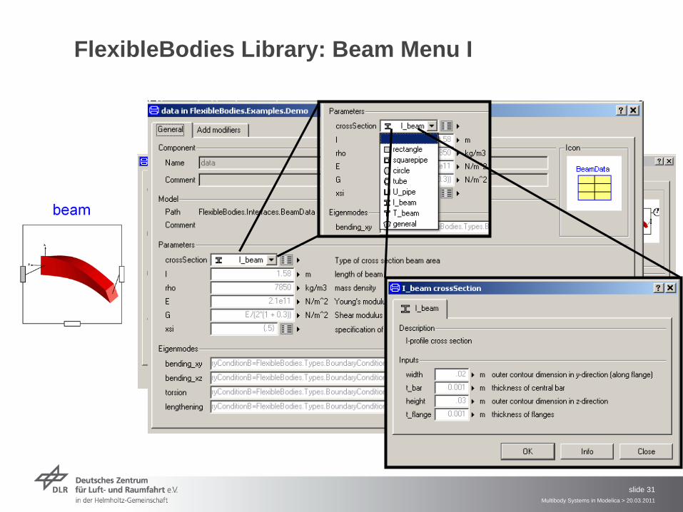
FlexibleBodies Library: Beam Menu I
Multibody Systems in Modelica > 20.03.2011
slide 32
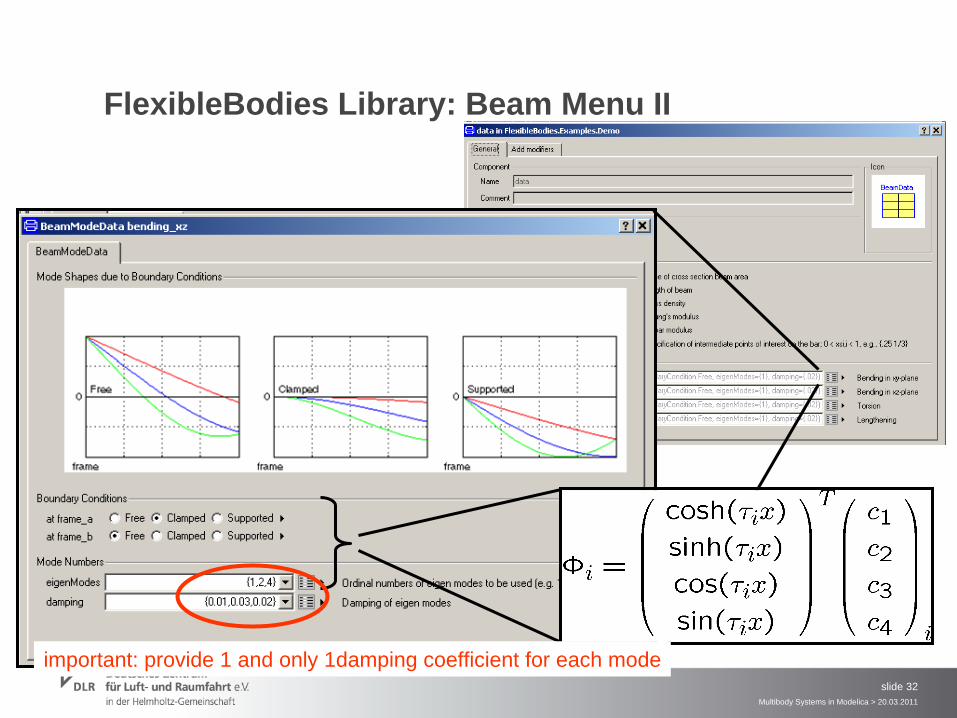
FlexibleBodies Library: Beam Menu II
important: provide 1 and only 1damping coefficient for each mode

Multibody Systems in Modelica > 20.03.2011
slide 33
Boundary Conditions I
1st Option: tangent frame: clamped-free b.c. correponds to cantilever beam
2nd Option: chord frame: supported-supported b.c.
3rd Option: Buckens frame: free-free b.c.
Linearisation: choose reference frame in such a way that is as small as possible
prefer Buckenssystem
(I)(R)
rR c
ur
see Schwertassek/Wallrapp/Shabana99

Multibody Systems in Modelica > 20.03.2011
slide 34
Boundary Conditions IIHelikopter-Rotor (see Examples/Beam)
choose the boundary conditions according to the attachment jointHeckmann2010: On the Choice of Boundary Conditions for Mode Shapes, Mulibody System Dynamics (23)

Multibody Systems in Modelica > 20.03.2011
slide 35
Exercise 3: The Flying Gull II
rectangle crosssectionwidth=0.12 height=0.005
l= 1m=1000 kg/m3E=1e9 N/m2 xsi={1/3}bending_xz
supported/free, {1}, {0.02}all other BeamModeData
fill(0,0), fill(0,0)

Multibody Systems in Modelica > 20.03.2011
slide 36
Exercise 4: a classic Pitfall IModel the following system
(quasi-) static deformation:a thrust-force shortens the beam
length= 1mE=1e10 N/m^2rectangular cross section 0.01 x 0.01 m1st eigenmode for lengthening deformationall other deformations are disregardedswitch off exaggerated animation Simulate 1000s with Radau5 !
Plot beam.frame_b.r_0[1] !

Multibody Systems in Modelica > 20.03.2011
slide 37
Exercise 4: a classic Pitfall II
beam
world
x
y
w orld
worldForce
ramp
duration=1000const
k=0w orld
worldForce1ba
n={1,0,0}actuatedPris...
spring
fixedTransl...
r={0,.1,0}a b
fixedTransl...
r={0,-.1,0}a b
relativeSen...a b
resol...
the system is now extended by an equivalent spring !
c=0.01m*0.01m*1e10 N/m^2 / (1 m)unstretched length = 1m
compare the deformationsby measurements !
Plot the relativeSensor.r_rel[1] !Gradually increase the number of modes !
Multibody Systems in Modelica > 20.03.2011
slide 38
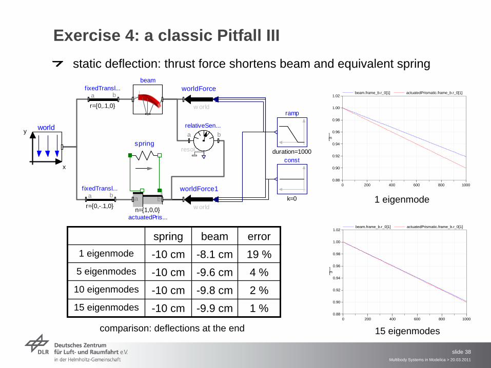
Exercise 4: a classic Pitfall III
beam
world
x
y
w orld
worldForce
ramp
duration=1000const
k=0w orld
worldForce1ba
n={1,0,0}actuatedPris...
spring
fixedTransl...
r={0,.1,0}a b
fixedTransl...
r={0,-.1,0}a b
relativeSen...a b
resol...
static deflection: thrust force shortens beam and equivalent spring
0 200 400 600 800 10000.88
0.90
0.92
0.94
0.96
0.98
1.00
1.02
[m]
beam.frame_b.r_0[1] actuatedPrismatic.frame_b.r_0[1]
1 eigenmode
0 200 400 600 800 10000.88
0.90
0.92
0.94
0.96
0.98
1.00
1.02
[m]
beam.frame_b.r_0[1] actuatedPrismatic.frame_b.r_0[1]
15 eigenmodes
spring beam error1 eigenmode -10 cm -8.1 cm 19 %5 eigenmodes -10 cm -9.6 cm 4 %
10 eigenmodes -10 cm -9.8 cm 2 %15 eigenmodes -10 cm -9.9 cm 1 %
comparison: deflections at the end

Multibody Systems in Modelica > 20.03.2011
slide 39
Exercise 4: a classic Pitfall IVMechanical background
static deflections rely on elastic properties only
eigenmodes consider elastic and interia properties
that‘s why they are well suited for dynamic problems
Geometrical background
analytically:
expansion with eigenmodes:
It is proven that Raleigh-Ritz approach converges against true value
but how fast ?
this is an extreme example, e.g. bending is less sensitive
Check whether a higher number of modes changes results !

Multibody Systems in Modelica > 20.03.2011
slide 40
Erxercise 5: unbalanced Shaft
15° around y-axis
circle Ø 0.05m l=1 m
1 xy- + 1xz- Bending mode supported-supported Ø 0.3m
Instability at which rotational velocity ?
Take care to initialize in stationary state ! (qdd(fixed=true),qd(fixed=true)
n_a={0,1,0}n_b={0,0,1}

Multibody Systems in Modelica > 20.03.2011
slide 41
Contents
Modelica Multibody BasicsExercise 1: Control of an inverse pendulumModelica Multibody AdvancedExercise 2: The Flying Gull IFlexibleBodies Library: BeamsExercise 3: The Flying Gull IIExercise 4: A classic PitfallExercise 5: Unbalanced ShaftFlexibleBodies Library: General bodies based on finite element dataExercise 6: The Flying Gull IIIFE-PreprocessingFlexibleBodies Library extensions at this conference

Multibody Systems in Modelica > 20.03.2011
slide 42
Recall Theory: the equations of motion
principle of virtual power
equations of motion: here
SID structure: definition of file format to file volume integrals
the generalized Newton-Euler-equations of motion of an unconstrained deformable body

Multibody Systems in Modelica > 20.03.2011
slide 43
SID-Data from FE: Where do they come from ?
Consider the linear FE-equation
the related eigenvalue problem
a set of eigenvectorsa selection of nodesfor each node mode shapes are collected from set of eigenvectors
the related rotational terms (non-volume-elements only)
the volume integrals are reassembled from (substructure) element inertia and stiffness data

Multibody Systems in Modelica > 20.03.2011
slide 44
FlexibleBodies Library: ModalBody Menu I

Multibody Systems in Modelica > 20.03.2011
slide 45
Exercise 6: The Flying Gull III1st step:
introduce world and ModalBody- modelassign SID-file …/Extras/Data/wing7.SID_FEMassign OBJ-file …/Extras/Data/wing.obj

Multibody Systems in Modelica > 20.03.2011
slide 46
Exercise 6: The Flying Gull III
Extras/Data/wing7.SID_FEMExtras/Data/wing.objNodes={69,76,80,91,102}
connect(sphericalSpherical.frame_b, wing1.nodes[3])

Multibody Systems in Modelica > 20.03.2011
slide 47
ModalBody example: 4-Cylinder-Engine
FEM-modelsCrankshaft : 106.789 nodesRod: 22777 nodes
Multibody representation< 1900 HzCrankshaft:
2 torsional eigenmodes305 simulation nodes
Rod4 eigenmodes each148 simulaltion nodes each
Time-integration with gas forces 38 states,6 cpu-s for 1 s

Multibody Systems in Modelica > 20.03.2011
slide 48
RealTime Modal Body
no external C-Code2. implementation( = parameter native=true) con‘s: not suitable for large models
no file accessSID-data filed as Modelica-record
dsmodel.c contains all code and all datano animation

Multibody Systems in Modelica > 20.03.2011
slide 49
Contents
Modelica Multibody BasicsExercise 1: Control of an inverse pendulumModelica Multibody AdvancedExercise 2: The Flying Gull IFlexibleBodies Library: BeamsExercise 3: The Flying Gull IIExercise 4: A classic PitfallExercise 5: Unbalanced ShaftFlexibleBodies Library: General bodies based on finite element dataExercise 6: The Flying Gull IIIFE-PreprocessingFlexibleBodies Library extensions at this conference

Multibody Systems in Modelica > 20.03.2011
slide 50
FE-preprocessing: in summary
1. FE-modelling2. generate wavefront–file (export mesh-information)3. prepare and select nodes to retain4. solve FE-eigenvalue problem
care for boundary conditions and frequency range5. generate FE- substructure6. generate SID-file FE-from substructure
7. introduce SID- and wavefront-file in Modelica

Multibody Systems in Modelica > 20.03.2011
slide 51
FE-preprocessing Step 2: wavefront-filethe animation file in wavefront format *.obj
an open (very) low level geometry formatfreely available tools existrepresents geometrical shape of the bobyinterpolation for animation is completely independent from MBS- simulationdue to limited animation performance,
the „outside“ geometry is sufficient, e.g. the mesh of the surface

Multibody Systems in Modelica > 20.03.2011
slide 52
FE-preprocessing Step 3: retained nodes
retained nodesprepare the body-model for interconnections of the MBS
select nodes where MBS-elements are supposed to be attached to
define of such nodes and associated MPCsconsider rotational degrees of freedom if needed
select an additional set of nodes necessary to support a „nice animation“
roughly equally distributed over surface of the bodyin most cases all together 200, 250 retained nodesyou may use the specific Abaqus comand line
*Nset SID_SELECTED_NODES

Multibody Systems in Modelica > 20.03.2011
slide 53
3 AttachmentPoints # 90000, 90003, 90006 on the axis line of the wheelset (to attach suspension and measurements devices)
12 AttachmentPoints at radius 460 y 750 equally distributed at thecircumference of each wheel (to introduce wheel/rail forces and torques )
y

Multibody Systems in Modelica > 20.03.2011
slide 54
FE-preprocessing Step 5: substructuringstandard FE-capability
Gyuan-, Craig-Bampton-…..methodAbaqus comand line
*SUBSTRUCTURE GENERATE, FLEXIBLE BODY=S-slength : scaling factor for the length unit (default: 1.0)-smass : scaling factor for the mass unit (default: 1.0)-stime : scaling factor for the time unit (default: 1.0)-fmin : lower boundary of the frequency range (default: 0.001Hz)-fmax : higher boundary of the frequency range (default: 1.E16Hz)-tol : zero cutoff tolerance (default - 1E-12)-help : this usage info
SID assumes SI units
alternative:number of modes
Multibody Systems in Modelica > 20.03.2011
slide 55
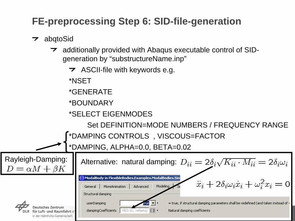
FE-preprocessing Step 6: SID-file-generationabqtoSid
additionally provided with Abaqus executable control of SID- generation by “substructureName.inp”
ASCII-file with keywords e.g.*NSET*GENERATE*BOUNDARY*SELECT EIGENMODES
Set DEFINITION=MODE NUMBERS / FREQUENCY RANGE*DAMPING CONTROLS , VISCOUS=FACTOR*DAMPING, ALPHA=0.0, BETA=0.02
Rayleigh-Damping: Alternative: natural damping:
Multibody Systems in Modelica > 20.03.2011
slide 56
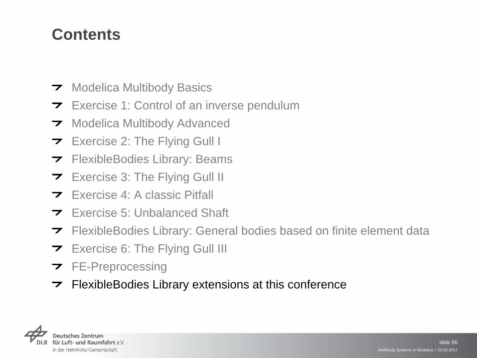
Contents
Modelica Multibody BasicsExercise 1: Control of an inverse pendulumModelica Multibody AdvancedExercise 2: The Flying Gull IFlexibleBodies Library: BeamsExercise 3: The Flying Gull IIExercise 4: A classic PitfallExercise 5: Unbalanced ShaftFlexibleBodies Library: General bodies based on finite element dataExercise 6: The Flying Gull IIIFE-PreprocessingFlexibleBodies Library extensions at this conference

Multibody Systems in Modelica > 20.03.2011
slide 57
FlexibleBodies Library extensions at this conferenceS. Hartweg, Monday HS3 12:00:
An Annular Plate Model in Arbitrary Lagrangian-Eulerian Description for the DLR FlexibleBodies Library
L . Reyes Perez, Monday HS2 15:35A thermoelastic annular plate model for the modeling of brake systems

Multibody Systems in Modelica > 20.03.2011
slide 58
Thank you very much for your attention !


![Dynamic Computation of Flexible Multibody System with ......rigid-flexible multibody systems by Tian et al. [12], who derived a new general and comprehensive approach for a spatial](https://static.fdocuments.in/doc/165x107/612a19a9b43f622fcf030d6d/dynamic-computation-of-flexible-multibody-system-with-rigid-flexible-multibody.jpg)
