Some Applications of Automatic Differentiation to

Rigid, Flexible, and Constrained Multibody

DynamicsD. T. Griffith

Sandia National Laboratories

J. D. Turner

Dynacs

J. L. Junkins

Texas A&M University

ASME 2005 International Design Engineering Technical Conferences

September 24, 2005

2

Folk theoremThe Chain Rule, when applied by hand

recursively to even moderately dimensioned nonlinear systems, for more than two orders of differentiation, stops being fun around age 45.

Empirical Evidence: The master differentiator, James Turner tried to automate the process

completely during his late forties.

3

Presentation Outline• Introduction to Automatic

Differentiation• Modeling

• Rigid and flexible multibody systems• Constrained multibody systems

• Automatic generation of exact PDE/ODEs and BCs for hybrid systems validation of approximate solutions

• Numerical Examples

4

Comparison of Computerized Differentiation Approaches

• Symbolic Differentiation– Very useful and popular – Matlab, Maple, Mathcad,

Macsyma– Pros: Can view expressions &

control simplification/ approximation on screen

– Cons: Result in lengthy expressions and require code generation/porting/de-bugging

• Automatic Differentiation (AD)– Generally, not as well-known as

Symbolic Differentiation– Recursive, automated use of Chain

Rule … – Begins with FORTRAN, C or …code

that computes the functions to be differentiated

– ADIFOR, AD01, ADOL-C, AUTODERIVE, OCEA

– Pro: Derivatives computed & possibly coded without (*much*) user intervention

– Historical Cons: Limited order of differentiation and also, usually requires code generation

OCEA is a novel AD approach that enables 1st- through 4th-order derivatives, with zero code generation required. There are very important implications in many fields, including multi-body dynamics.

5

Overview of automatic differentiation by OCEA (1)

– OCEA (Object Oriented Coordinate Embedding Method)– Define new data structure (OCEA second-order method), for example for the

function scalar f :

– All intrinsic operators ( +, - , * , / , = ) are overloaded to enable, for example, addition and multiplication of OCEA variables. Examples:

You code: OCEA computes:

– Composite Functions (chain rule, use recursively, numerically!): You code: OCEA computes:

– Let’s take a look at an illustrative example….

2 21 2 1 2 1 2 1 2:f f f f f f f f

2 21 2 1 2 1 2 1 2 1 2 1 2 1 2* : * * * * 2 * *Tf f f f f f f f f f f f f f

2( ) :f f f f x

2

2 22

: , , : , ,Tf f f

f g f g g g f g g g g gg g g

6

Overview of automatic differentiation by OCEA (2)

• A second-order OCEA example• Suppose:

OCEA-FORTRAN

! X(1) = x, X(2) = y

Type(EB):: X(2)

Type(EB):: F1, F2, F3

Real(DP):: S_F3, JAC_F3(2), HES_F3(2,2)

! Code Functions

F1 = X(1)**3 + X(2)

F2 = (X(2)**2)*sin( X(1) )

F3 = F1 + F2

S_F3 = F3 ! Extract function

JAC_F3 = F3 ! Extract Jacobian (2x1)

HES_F3 = F3 ! Extract Hessian (2x2)

Declare OCEA independent variables , type EB

Declare OCEA dependent variables, type EB

Declare function and partial derivative arrays , type DP

Code functions

Extract partial derivative

information

2 23 1 2 1 2 1 2

23 3 3

:

:

f f f f f f f

f f f

function Jacobian Hessian

We desire tocompute f3 and most

importantly its partials:

3 21 2 3 1 2, sin( ),f x y f y x and f f f

2 23 33

22 2 2

2 23 3 3

2

3 cos 6 sin 2 cos,

1 2 sin 2 cos 2sin

f ffx x yx y x x y x y xx

f y x y x xf fy x y y

You never had to derive, code, or debug:

7

Equation of motion formulation using automatic differentiation

Lagrange’s equations:

Td L LC

dt

Q λq q

C q bsubject to

Lagrangian:

T, V: kinetic and potential energy

q: generalized coordinates

Q: generalized force

C(q): constraint Jacobian matrix

: Lagrange multipliers

L T V

Of course, many choices for equation of motion formulation exist.

The OCEA approach is broadly applicable, however, the utility of automatic differentiation can be immediately seen and appreciated for implementing Lagrange’s Equations…

8

Implementation of Lagrange’s Equations:

A Direct Approach (1)

Td T LC

dt

Q λq q

2 2

j ji i j i j

d T T Tq q

dt q q q q q

2

iji j

TM m

q q

2

iji j

TM m

q q

Td L LC

dt

Q λq q

L

C

L

q

Q

Automatic Differentiation (AD)

Specified & coded

AD or specified & coded

Many numerical methods

AD or specified & coded

Mass matrix and its time derivative extracted as second-order Automatic Differentiation of T …

9

Implementation of Lagrange’s Equations:

A Direct Approach (2)2

iji j

TM m

q q

2

iji j

TM m

q q

( , )t q 0

( , )t C Ct t

q q = q 0q q

TLM M C

q + q Q λq

-1 TLM M C

q = q + Q λ

q

Can also compute constraint matrix, C, automatically for holonomic type constraint.

Now forming the equations:

Accelerations computed after generating or prescribing all terms here. Now, can proceed with numerical integration…….

10

Illustrative Example: Spring Pendulum (1)

L T V 2 2 212 ( )T m r r

210 02 ( ) ( cos )V k r r mg r r

2

( ) iji j

TM m

q q

q

2

( ) iji j

TM m

q q

q

-1 TLM M C

q = q + Q λ

q

r

θ

Lagranges Eqs:

Directly invoke ODE solver in OCEA to get solution W/O hand derivation, coding, or checkout … only derive & code T, V

11

Spring Pendulum (2)SUBROUTINE SPRING_PEND_EQNS( PASS, TIME, X, DXDT, FLAG )

USE EB_HANDLINGIMPLICIT NONE

****************************************!.....LOCAL VARIABLES

TYPE(EB)::L, T, V ! LAGRANGIAN, KINETIC, POTENTIALREAL(DP):: M, K ! MASS AND STIFFNESS VALUESREAL(DP), DIMENSION(NV):: JAC_LREAL(DP), DIMENSION(NV,NV):: HES_L

****************************************! X(1) = Q(1) = R, X(2) = Q(2) = THETA, X(3) = dR/dt, X(4) = dTHETA/dtR0 = 0.55D0GRAV = 9.81D0T = 0.5D0*M*(X(3)**2 + X(1)**2*X(4)**2) ! DEFINE KEV = 0.5D0*K*(X(1)-R0)**2 + M*GRAV*(R0-X(1)*COS(X(2))) ! DEFINE PEL = T – V ! DEFINE LAGRANGIAN FUNCTION

JAC_L = L ! EXTRACT dL/(dq,dqdot)JAC_L_Q = JAC_L(1:NV/2) ! EXTRACT dL/dq

HES_L = L ! EXTRACT 2nd ORDER PARTIALS OF LAGRANGIANMASS = HES_L(NV/2+1:NV,NV/2+1:NV) ! EXTRACT MASS MATRIXMASSDOT = HES_L(NV/2+1:NV,1:NV/2) ! EXTRACT MDOT! QDOTDOT = INV(MASS)*(- MASSDOT*Q + JAC_L_Q ) ! SEE PAPER …

****************************************DXDT(1)%E = X(3)%E ! RDOTDXDT(2)%E = X(4)%E ! THETADOTDXDT(3)%E = QDOTDOT(1) ! RDOTDOTDXDT(4)%E = QDOTDOT(2) ! THETADOTDOT

END SUBROUTINE SPRING_PEND_EQNS

12

Geometry of Multiple Flexible Link Configuration

Note from the figure of a series of deformed links that the local coordinate frames attached to the links are defined such that the elastic deformation vanishes at the endpoints. This choice greatly simplifies the “downstream” velocity expressions.

1

1̂j

1̂i

ˆp+1j

2

2̂iˆ

2j

1p

ˆp+1i

13

Kinetic Energy Generalization for Flexible Links

1

1 1 1 1 1 1 1 10

1( ) ( , ) ( , )

2

pL

p p p p p p p pT x x t x t dx

r r

1 1

11 1 1 1 12

1 1 1

11 1 1 1 1 1 12

1 1

21 11 1 1 1 1 1 12 2

( , , , )

cos sin

cos cos

p p

p p pT

p i i j j j i p p p i i p ii j i

p pT

p p i i p i p p p i i p ii i

T T

p p p p p p p

T T

m L L L

L m L L

M M

q q θ θ

q b

q b

q q q q

2 211 1 1 1 1 16

T

p p p p p pm L q a

Assumed Modes Method used to transform the kinetic energy expression into a form which can be tamed by Lagrange’s Equations. The details can be found in the paper.

Along with the potential energy expression, we can define the Lagrangian and proceed to generate the equations of motion…………..

14

Example: Closed-chain 5-link Manipulator (1)

5cos( )

15

sin( )1

L Di ii

Li ii

φ = 0

The Lagrangian expressions are developed for each link and summed to form the total system Lagrangian.

Additionally, we specify two holonomic constraints of the form:

And, we specify damping at all joints with the exception of the base end of link 5.

OCEA automatically generates the equations of motion for the constrained

system

5 link manipulator g D

1

2

3

4

5

15

Example: Closed-chain 5-link Manipulator (2)

16

Example: 4-link Planar Truss (1)

Y

4cos( )

14

sin( )1

Li ii

Li ii

φ = 0

The Lagrangian expressions are developed for each link and summed to

form the total system Lagrangian.

Now, we consider translation as well.

Additionally, we specify two holonomic constraints of the form:

OCEA automatically generates the equations of motion for the constrained

system

4-link planar truss with “springs” across diagonal

X

1

2

3

4

17

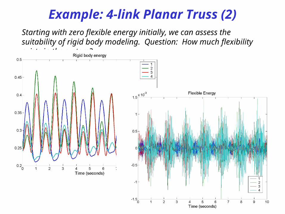
Example: 4-link Planar Truss (2)Starting with zero flexible energy initially, we can assess the suitability of rigid body modeling. Question: How much flexibility exists in the system?

20

Accuracy of Solutions: Comparison with Hard-coded Equations of Motion for Flexible

Double Pendulum(1)

Angular coordinates and angular velocities

21

Accuracy of Solutions: Comparison with Hard-coded Equations of Motion

for Double Pendulum(2)

Flexible coordinates for link one

22

Methods for Validating Solution Accuracy

1) Testing special cases that have exact analytical solutions

2) Evaluation of error in exact motion integrals

3) The method of manufactured solutions

4) The method of “nearby problems”

Method #1 is a standard approach to validating solution accuracy. Here we look at a simple system which has an exact analytical solution.

Methods #3 and #4 rely upon computing analytical source terms (fictitious generalized forces) by inverse dynamics which define a benchmark problem for validation studies. The difference is that with method #3 a benchmark solution is chosen a priori and may have no important physical meaning. With method #4, a benchmark solution is constructed as a neighbor of a candidate approximate solution for the motion being studied and thus has physical meaning.

27

Addendum to JLJ Folk Theorem

Generating the exact ODE/PDE and boundary conditions for a distributed parameter system

by hand or symbolic manipulation stops being fun at

age 29!

28

Generating Exact PDE/ODEs and BCs for Many Body Distributed Parameter

Systems1 0

2

2

0

ˆ

ˆ ˆ ˆ ˆˆ

' ''

ˆ ˆ

' ''

( ) ( )

i

i

ln

D i i Bi

T

Ti i i ii

i i i ii i

l

i ii

ii i

B B

i i i i

L L dx L

d

dt

L L L Ld

dt v v x xv v

L Lv

xv v

d

v l dt v l

Qq q

f

L

L L

L L 1

2

0

ˆ( ) ( ) 0

ˆ ' ' 'ˆ( ) ( ) 0'' ' '( ) ( )

i

Ti i i i i

l

Ti B Bi i i i i i

i i i i i

v l v l

L dv v l v l

dtv v l v l

f

f

L L

Lagrangian:

Discrete/ODE:

Flexible/PDE:

BCs:

You code this.

OCEA/AD computes these.

31

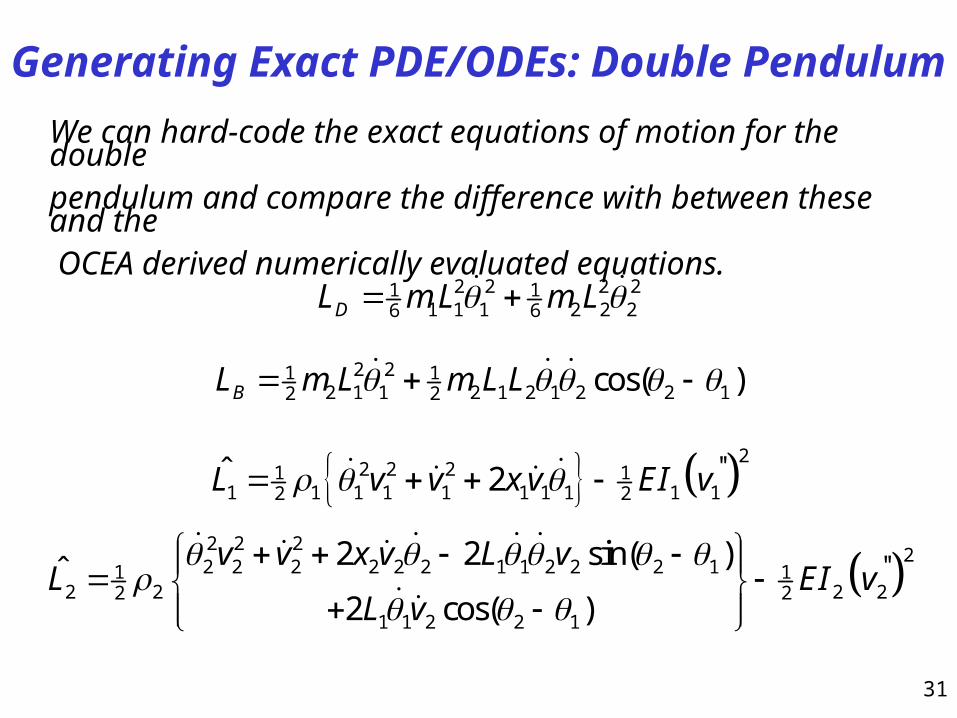
Generating Exact PDE/ODEs: Double Pendulum

We can hard-code the exact equations of motion for the doublependulum and compare the difference with between these and the OCEA derived numerically evaluated equations.

2 2 2 21 11 1 1 2 2 26 6DL m L m L

2 21 12 1 1 2 1 2 1 2 2 12 2 cos( )BL m L m L L

22 2 21 1

1 1 1 1 1 1 1 1 1 12 2''ˆ 2L v v x v EI v

2 2 2

22 2 2 2 2 2 1 1 2 2 2 11 1

2 2 2 22 2

1 1 2 2 1

''2 2 sin( )ˆ2 cos( )

v v x v L vL EI v

L v

32

Errors in ODEs: Double Pendulum

33

Errors in PDEs: Double Pendulum

Link one

Link two

34

Summary and Conclusions

•Automatic Differentiation has broad potential in Dynamics and Control

• Automating differentiation by operator overloading is a beautiful idea whose time has come – the applications are endless!

• Ideal for implementing Lagrange’s Equations – this presentation provides some simple illustrations – a few important first steps along the path.

• No hand derivation effort beyond code specifying the building of the Lagrangian, constraints and external forces is required.

• OCEA also gives rise to new methods for solving differential equations – the time derivative computations can be automated, so that formal analytical continuation is easily done in lieu of traditional Runge-Kutta methods, for example.

• Can automatically derive systems of PDEs and BCs for use in validating the accuracy of approximate solutions of flexible systems corresponding to the same modeling assumptions?