Abstract Number: 007-0141

Modelling and analysis of an Integrated Automated Guided Vehicle

System using CPN and RSM.

Tauseef Aized, Doctoral candidate, Hagiwara Lab, Mechanical Sciences and Engineering Department, email: tauseef.aa@m.titech.ac.jp Koji Takahashi, Associate Professor, Takahashi Lab, Electrical and Electronic Engineering Department, email: koji@ee.titech.ac.jp Ichiro Hagiwara, Professor, Hagiwara Lab, Mechanical Sciences and Engineering Department email: Hagiwara@mech.titech.ac.jp

Tokyo Institute of Technology, 2-12-1 Ookayama, Meguro-Ku, Tokyo 152-8550, Japan.

POMS 18th Annual Conference, Dallas, Texas, U.S.A. , May 4 to May 7, 2007

Summary:

The objective of this study is to analyse an integrated Automated Guided Vehicle System (AGVS)

which is embedded in a pull type multi-product, multi-stage, multi-line Flexible Manufacturing System

(FMS). This study analyses the guide path configurations of the AGVS. For this purpose, three

different guide path configurations have been developed and their impact on the performance of the

Flexible manufacturing system has been presented. The system is modelled using coloured Petri net

(CPN) methodology and the study has been extended to seek near-optimal conditions of the

configurations using Response surface method (RSM).

Key words:

automated guided vehicle system, flexible manufacturing system, guide path configurations, coloured

Petri net, multiple response optimization, response surface method

2

1. Introduction:

In modern manufacturing environments, automated guided vehicle systems have become an integral

part of overall manufacturing systems. An AGVS contains one or more automated guided vehicles

which are driverless vehicles used for horizontal movement of materials. AGVs are commonly used in

facilities such as manufacturing plants, distribution centres, warehouses and transhipments. The AGVS

studied in this paper is a discrete event dynamical system (DEDS) which is event driven, asynchronous

and non-deterministic in nature. Petri net are powerful techniques to model such systems in that they

can handle complex system modelling concepts and constraints. Moreover, coloured Petri net (CPN)

provides compact models of large systems with a higher level of abstraction [1]. Hence, this study uses

CPN method for modelling the system and the data generated by the CPN model are used to develop

the response surface models to explore near-optimal conditions of the system.

2. Related work and originality:

The majority of the research work available in FMS modelling literature considers only the modelling

of materials processing through work centres and assumes uninterrupted availability of material

handling equipment. This could be valid for conveyorized production system but it is not reasonable

for AGV-based systems [2]. Several researchers have stressed that efficient scheduling of material

handling system is critical to the overall efficiency of FMS [3]. The integration of material handling

system (MHS) with manufacturing activities can result in manufacturing systems characterized by

flexibility, high productivity and low cost per unit produced [4]. Also, to achieve global optimization

between material processing and material handling activities, manufacturing planning should consider

these two functions simultaneously [5]. Nevertheless, the integration of MHS with FMS inevitably

increases the complexity of the problem as it comprises inseparable decisions for both material

3

processing and material handling activities [2].The design and control processes of an AGVS involve

many issues like guide-path design, traffic management, vehicle requirements, dispatching, routing and

scheduling [6]. Among these factors, guide-path or flow-path configuration design can be seen as a

problem at strategic level [7]. The guide-path layout influences the performance of a system as it

impacts the travel time to transport a load from its origin to its destination, the number of vehicles

required and the degree of congestion [6]. The most common performance criterion in guide-path

design is minimizing the total vehicle travel distance corresponding to given layout and flows [8], [9].

The direction of AGVs’ travel along guide-path may be unidirectional, bidirectional or a mix of

unidirectional and bidirectional paths [6]. The configuration of mixed unidirectional and bidirectional

flow paths is studied in [10] with the purpose to reduce travel distance. It indicates that benefits can be

obtained in throughput rates and in the size of vehicle fleet whereas the rate of vehicle congestion

increases and traffic control becomes more important. The simulation methodology has been used to

model traditional, tandem and tandem/loop configurations in [11] and the benefits and limitations of

each configuration have been discussed.

The contribution of this study is that it analyses the impact of flexibility on the performance of an

integrated AGVS through the development of different guide-path configurations. The configurations

are developed in such a way that flexibility, defined in terms of guide path configurations design to

accommodate varying number of AGVs, is gradually enhanced and its impact on system performance

is examined in order to propose the best configuration. The details of the configurations are discussed

in section 4. The problem of AGV congestion as discussed earlier [10] is solved through a suitable

control policy for the FMS. Also, this study is extended to seek global near-optimal performance in

each configuration and the configurations are compared to propose the best performance of the

4

manufacturing system. The system is modelled through CPN method and response surface method

(RSM) is implemented in order to achieve the best performance of the system. The joint use of CPN

and RSM can be taken as a general methodology for modelling, analysis and optimization of a discrete

event dynamical system. Moreover, this study presents the application of advanced tools like CPN

Tools and Design Expert and shows how these powerful tools can be used to model, analyse and

optimize a manufacturing system.

3. Coloured Petri net (CPN):

This study uses the definition of CPN given in [12].A hierarchical CPN is a tuple HCPN= (S, SN, SA,

PN, PT, PA, FS, FT, PP) satisfying the following requirements

1. S is a finite set of pages such that:

Each page s ∈ S is a non-hierarchical CPN:

CPN= (∑s, Ps, Ts, As, Ns, Cs, Gs, Es, Is)

(The non-hierarchical CPN is defined in [12])

2. The sets of net elements are pair wise disjoint:

∀ s1, s2 ∈ S: [s1 ≠ s2 � (Ps1 ∪ Ts1 ∪ As1) ∩ ( Ps2 ∪Ts2∪ As2 ) = ø ].

SN � T is a set of substitution nodes.

3. SA is a page assignment function. It is defined from SN into S such that: No page is a sub page of

itself:

{ s0 s1 …sn ∈ S*| n ∈ N+ �s0=sn �∀k ∈ 1..n: sk ∈ SA ( SNsk-1)}= ø.

4. PN � P is a set of port nodes.

5. PT is a port type function. It is defined from PN into {in, out, i/o, general}.

5

PA is a port assignment function, FS � Ps is a finite set of fusion sets, FT is a fusion type function and

PP ∈ SMs is a multi-set of prime pages. For details of PA, FS and FT, we refer to [12].

4. AGVS configurations:

This study integrates the AGVS with our previously developed FMS whose details are given in [13]

and extends our study [14] by finding near-optimal conditions of the AGVS. The previously developed

FMS has two manufacturing and one assembly cells where as each manufacturing cell has two

production lines, each line comprising of three machines, and the assembly cell has two assembly

stations. The integrated AGVS is analysed through the development of three guide-path

configurations . These configurations range from rigidly dedicated to flexible relationships between

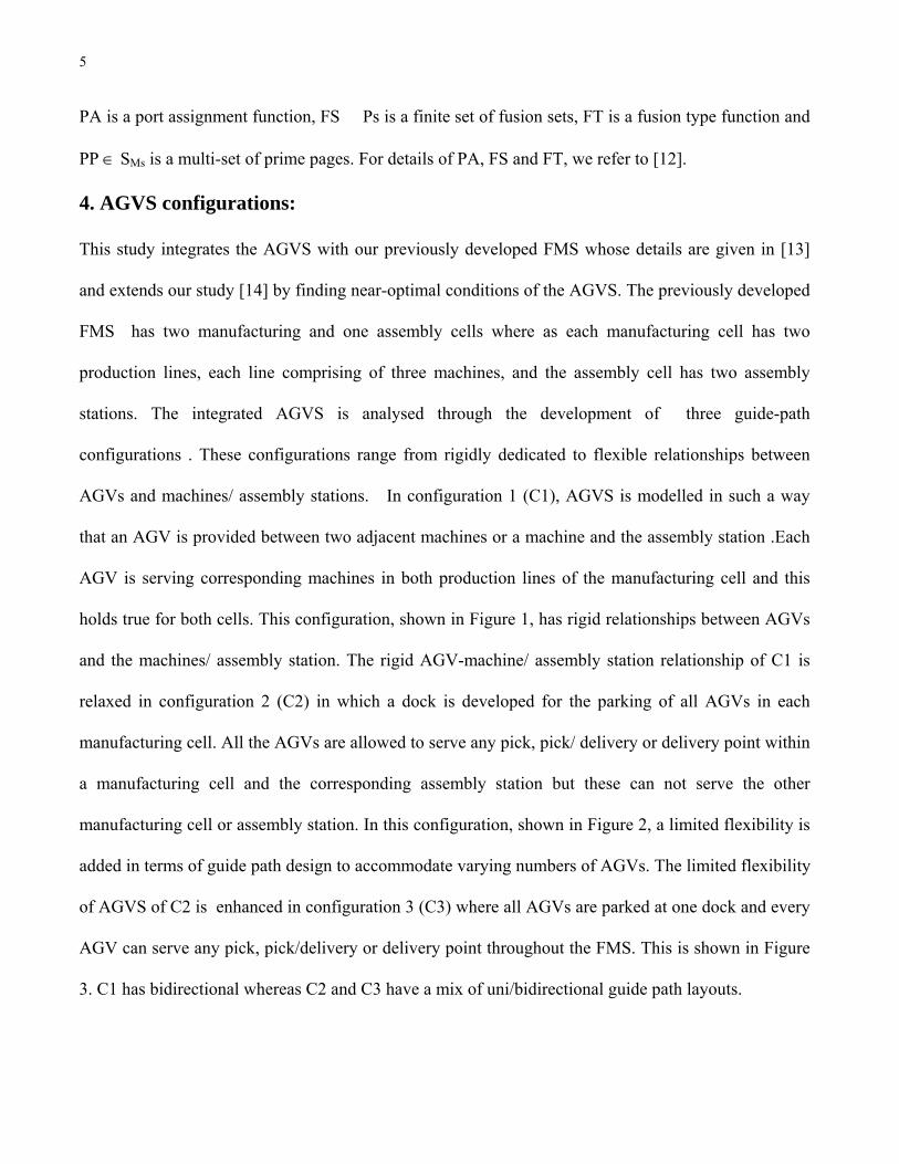
AGVs and machines/ assembly stations. In configuration 1 (C1), AGVS is modelled in such a way

that an AGV is provided between two adjacent machines or a machine and the assembly station .Each

AGV is serving corresponding machines in both production lines of the manufacturing cell and this

holds true for both cells. This configuration, shown in Figure 1, has rigid relationships between AGVs

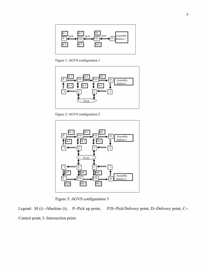
and the machines/ assembly station. The rigid AGV-machine/ assembly station relationship of C1 is

relaxed in configuration 2 (C2) in which a dock is developed for the parking of all AGVs in each

manufacturing cell. All the AGVs are allowed to serve any pick, pick/ delivery or delivery point within

a manufacturing cell and the corresponding assembly station but these can not serve the other

manufacturing cell or assembly station. In this configuration, shown in Figure 2, a limited flexibility is

added in terms of guide path design to accommodate varying numbers of AGVs. The limited flexibility

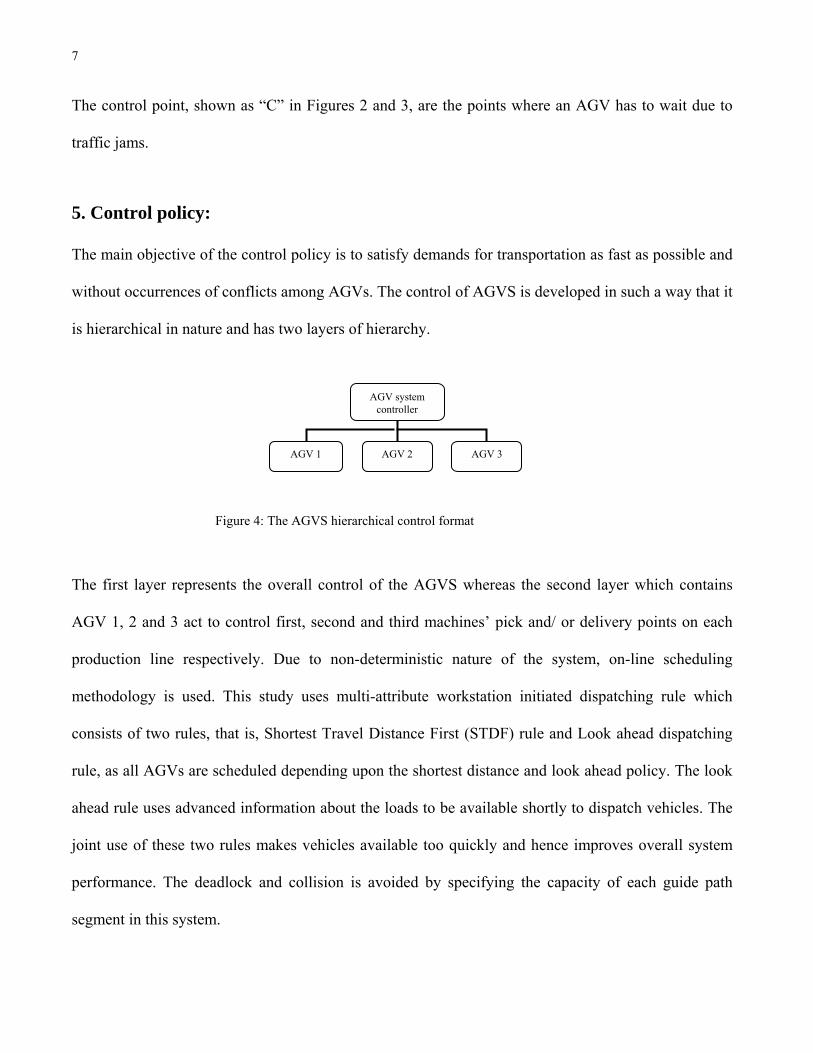
of AGVS of C2 is enhanced in configuration 3 (C3) where all AGVs are parked at one dock and every

AGV can serve any pick, pick/delivery or delivery point throughout the FMS. This is shown in Figure

3. C1 has bidirectional whereas C2 and C3 have a mix of uni/bidirectional guide path layouts.

6

Figure 1: AGVS configuration 1

Figure 2: AGVS configuration 2

Figure 3: AGVS configuration 3

Legend: M (i) --Machine (i), P--Pick up point, P/D--Pick/Delivery point, D--Delivery point, C--

Control point, I--Intersection point.

M 1

P/D Assembly Station 1

M 2 M3

M 4 M 5 M 6

P/D P DAGV AGV AGV

Assembly Station 1

DP/D P/D M 1 M 2 M3

M 4 M 5 M 6

I IC C

P

Dock

Assembly Station 1

DP/D P/D M 1 M 2 M3

M 4 M 5 M 6

I IC C

P

Dock

I IC C

DP/D P/D P

M10 M11 M12

M7 M8 M9 Assembly Station 2

7

The control point, shown as “C” in Figures 2 and 3, are the points where an AGV has to wait due to

traffic jams.

5. Control policy:

The main objective of the control policy is to satisfy demands for transportation as fast as possible and

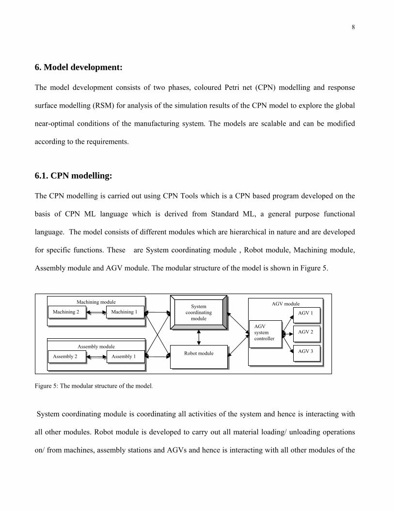
without occurrences of conflicts among AGVs. The control of AGVS is developed in such a way that it

is hierarchical in nature and has two layers of hierarchy.

Figure 4: The AGVS hierarchical control format

The first layer represents the overall control of the AGVS whereas the second layer which contains

AGV 1, 2 and 3 act to control first, second and third machines’ pick and/ or delivery points on each

production line respectively. Due to non-deterministic nature of the system, on-line scheduling

methodology is used. This study uses multi-attribute workstation initiated dispatching rule which

consists of two rules, that is, Shortest Travel Distance First (STDF) rule and Look ahead dispatching

rule, as all AGVs are scheduled depending upon the shortest distance and look ahead policy. The look

ahead rule uses advanced information about the loads to be available shortly to dispatch vehicles. The

joint use of these two rules makes vehicles available too quickly and hence improves overall system

performance. The deadlock and collision is avoided by specifying the capacity of each guide path

segment in this system.

AGV system controller

AGV 1 AGV 2 AGV 3

8

6. Model development:

The model development consists of two phases, coloured Petri net (CPN) modelling and response

surface modelling (RSM) for analysis of the simulation results of the CPN model to explore the global

near-optimal conditions of the manufacturing system. The models are scalable and can be modified

according to the requirements.

6.1. CPN modelling:

The CPN modelling is carried out using CPN Tools which is a CPN based program developed on the

basis of CPN ML language which is derived from Standard ML, a general purpose functional

language. The model consists of different modules which are hierarchical in nature and are developed

for specific functions. These are System coordinating module , Robot module, Machining module,

Assembly module and AGV module. The modular structure of the model is shown in Figure 5.

Figure 5: The modular structure of the model.

System coordinating module is coordinating all activities of the system and hence is interacting with

all other modules. Robot module is developed to carry out all material loading/ unloading operations

on/ from machines, assembly stations and AGVs and hence is interacting with all other modules of the

System coordinating

module

Robot module

Machining module Machining 2 Machining 1

Assembly module

Assembly module Assembly 2 Assembly 1

AGV module

AGV system controller

AGV 1

AGV 2

AGV 3

9

model. Machining module is responsible for all machining operations and consists of two sub modules,

Machining 1 and Machining 2. Machining 1 is carrying out all machining operations and machining 2

is developed to implement routing flexibility regarding material flow. Assembly module is

accomplishing all assembly operations and has two sub modules called Assembly 1 and Assembly 2.

Both assembly sub modules are developed to carry out assembly operations and also contain the

provisions to use alternate assembly stations in case of breakdown of an assembly station. The AGV

module is responsible for all material transportation activities and consists of four sub modules which

are AGV system controller, AGV 1, AGV 2 and AGV 3. AGV module is developed to implement the

control policy and the guide path configuration design of the AGVS and can be modified in order to

implement any of the stated guide path configurations. All transportation operations are modelled

using exponential distribution functions.

6.2 Response surface modelling:

Response surface method (RSM) is a planned approach for determining cause and effect relationships

and can be used for studying more than one input factor in a single experiment [15]. Derringer and

Suich [16] described a multiple response method which makes use of an objective function, called

desirability function. The general approach is to first convert each response into an individual

desirability function di that varies over the range, 0≤di≤1, where if the response is at the goal or target,

then di= 1 and if the response is outside an acceptable region, then di = 0. The simultaneous objective

function is a geometric mean of all transformed responses and is given by:

nn

ii

nn ddddD

1

1

1

21 )...(⎟⎟⎟

⎠

⎞

⎜⎜⎜

⎝

⎛=×××= ∏

=

10

Where n is the number of responses. If any of the responses fall outside its desirability range, the

overall function becomes zero. For simultaneous optimization each response must have a low value (lv)

and a high value (hv) assigned to each goal, such that for maximum goal:

di = 0 if yi < lv , 0≤di≤1 if lv ≤ yi ≤ h v , di = 1 if yi > hv

and for minimum goal:

di = 1 if yi < lv , 1 ≥ di ≥ 0 if lv ≤ yi ≤ hv , di = 0 if yi> hv

In desirability function, each response can also be assigned an importance relative to the other

responses. Importance (ri) varies from the least important to the most important. By assigning different

importance to different responses, the objective function is given by:

( ) ∑⎟⎟⎟

⎠

⎞

⎜⎜⎜

⎝

⎛=×××= ∏

=

irn

i

irinnr

nrr ddddD

1

1

12

21

1 ...

The shape of desirability function also changes with the addition of weights function which is used to

emphasize upper or lower bounds. RSM modelling and analysis have been carried out using Design

Expert 7.0.2 tool.

7. Simulation results and discussion:

The following are the simulation assumptions:

• The lengths of all guide path segments are the same.

• When an AGV enters into any guide path segment, it will continue travelling till the end of the

segment.

• The AGV speed for all segments of the guide path is the same.

11

Before collecting the resulting data, it is important to detect warm-up period to access steady state

behaviour of the system. This study uses four stage SPC approach [15] to find out steady state results.

As the input factors vary for individual simulation runs in this study, hence the warm-up period is also

varying depending on the particular input factor settings. In general, we have carried out ten

independent replication for each input factor settings and have determined the warm-up period. This

period has been excluded while collecting the data from the simulation runs and the length of the

steady state period has been determined according to the recommendations given in [15].Hence, the

simulation results are repeatable. The overall performance of the system is measured through material

processing system and material handling system measures. The material processing or FMS measures

include mean throughput ( number of products/ day) and mean cycle Time (number of minutes)

whereas material handling or the AGVS measures include mean AGV utilization ( percentage of total

time), mean AGV response time (number of minutes) and mean AGV congestion ( percentage of total

time). Mean AGV utilization is defined as the percentage of total time for which an AGV is used to

transport a load from one location to another. In cases of C2 and C3, the AGV move time associated in

moving to claim a load is included in utilization calculations. Mean AGV response time is defined as

the mean time from the moment when an AGV is called up by a workstation to the moment when the

AGV is available at the nearest pick-up point of that workstation for carrying the load. AGV

congestion is defined as the percentage of total time that an AGV waits at a control point due to traffic

jams. The numbers of AGVs in C1 are six which is a fixed number as C1 has a rigidly dedicated

AGVS format. C2 has two fleet of AGVs, each fleet is serving a specific manufacturing and relevant

assembly station and an addition of one AGV in each fleet results two more AGVs in the AGVS.

Hence, the numbers of AGVs begin from two and can increase with a multiple of two in the AGVS.

For the simulation experiments, the numbers of AGVs are ranging from two to eight. C3 has the most

12

flexible guide path design and the number of AGVs can range from one to any multiple of one; for the

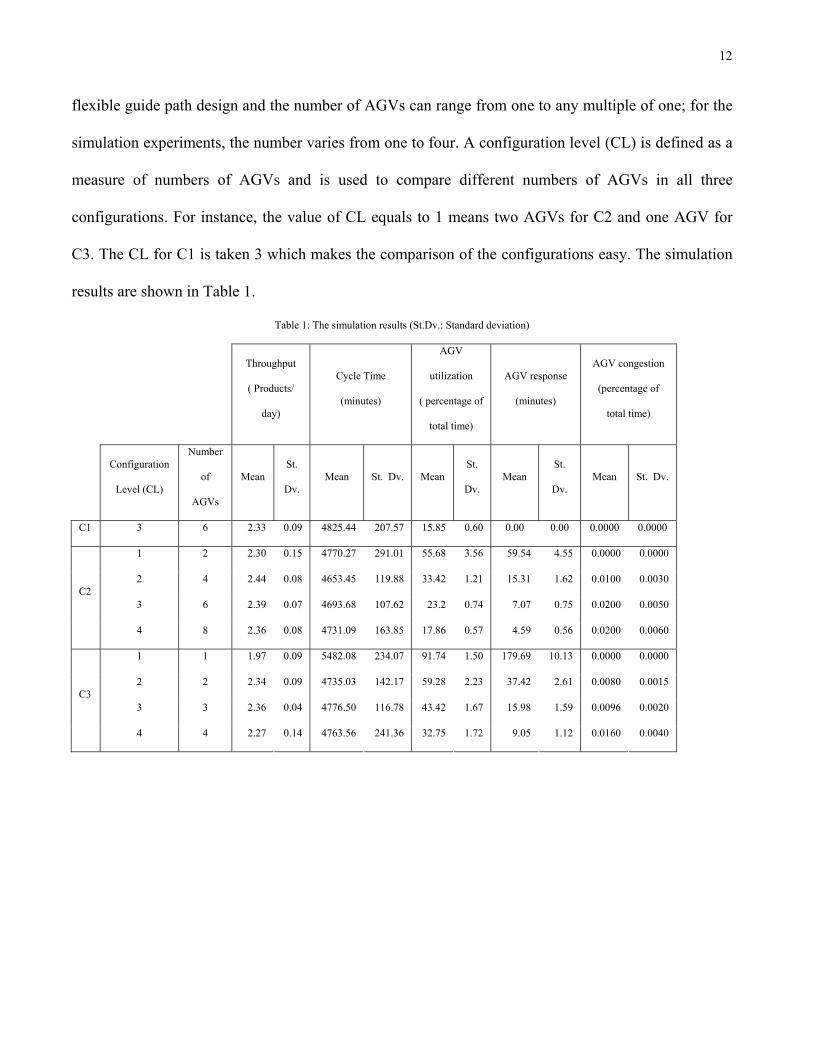
simulation experiments, the number varies from one to four. A configuration level (CL) is defined as a

measure of numbers of AGVs and is used to compare different numbers of AGVs in all three

configurations. For instance, the value of CL equals to 1 means two AGVs for C2 and one AGV for

C3. The CL for C1 is taken 3 which makes the comparison of the configurations easy. The simulation

results are shown in Table 1.

Table 1: The simulation results (St.Dv.: Standard deviation)

Throughput

( Products/

day)

Cycle Time

(minutes)

AGV

utilization

( percentage of

total time)

AGV response

(minutes)

AGV congestion

(percentage of

total time)

Configuration

Level (CL)

Number

of

AGVs

Mean St.

Dv. Mean St. Dv. Mean

St.

Dv. Mean

St.

Dv. Mean St. Dv.

C1 3 6 2.33 0.09 4825.44 207.57 15.85 0.60 0.00 0.00 0.0000 0.0000

1 2 2.30 0.15 4770.27 291.01 55.68 3.56 59.54 4.55 0.0000 0.0000

2 4 2.44 0.08 4653.45 119.88 33.42 1.21 15.31 1.62 0.0100 0.0030

3 6 2.39 0.07 4693.68 107.62 23.2 0.74 7.07 0.75 0.0200 0.0050 C2

4 8 2.36 0.08 4731.09 163.85 17.86 0.57 4.59 0.56 0.0200 0.0060

1 1 1.97 0.09 5482.08 234.07 91.74 1.50 179.69 10.13 0.0000 0.0000

2 2 2.34 0.09 4735.03 142.17 59.28 2.23 37.42 2.61 0.0080 0.0015

3 3 2.36 0.04 4776.50 116.78 43.42 1.67 15.98 1.59 0.0096 0.0020 C3

4 4 2.27 0.14 4763.56 241.36 32.75 1.72 9.05 1.12 0.0160 0.0040

0

0.5

1

1.5

2

2.5

3

0 1 2 3 4 5

Configuration Level

Thro

ughp

ut C1C2C3

4000

4800

5600

0 1 2 3 4 5

Configuration Level (CL)

Cyc

le T

ime

C1C2C3

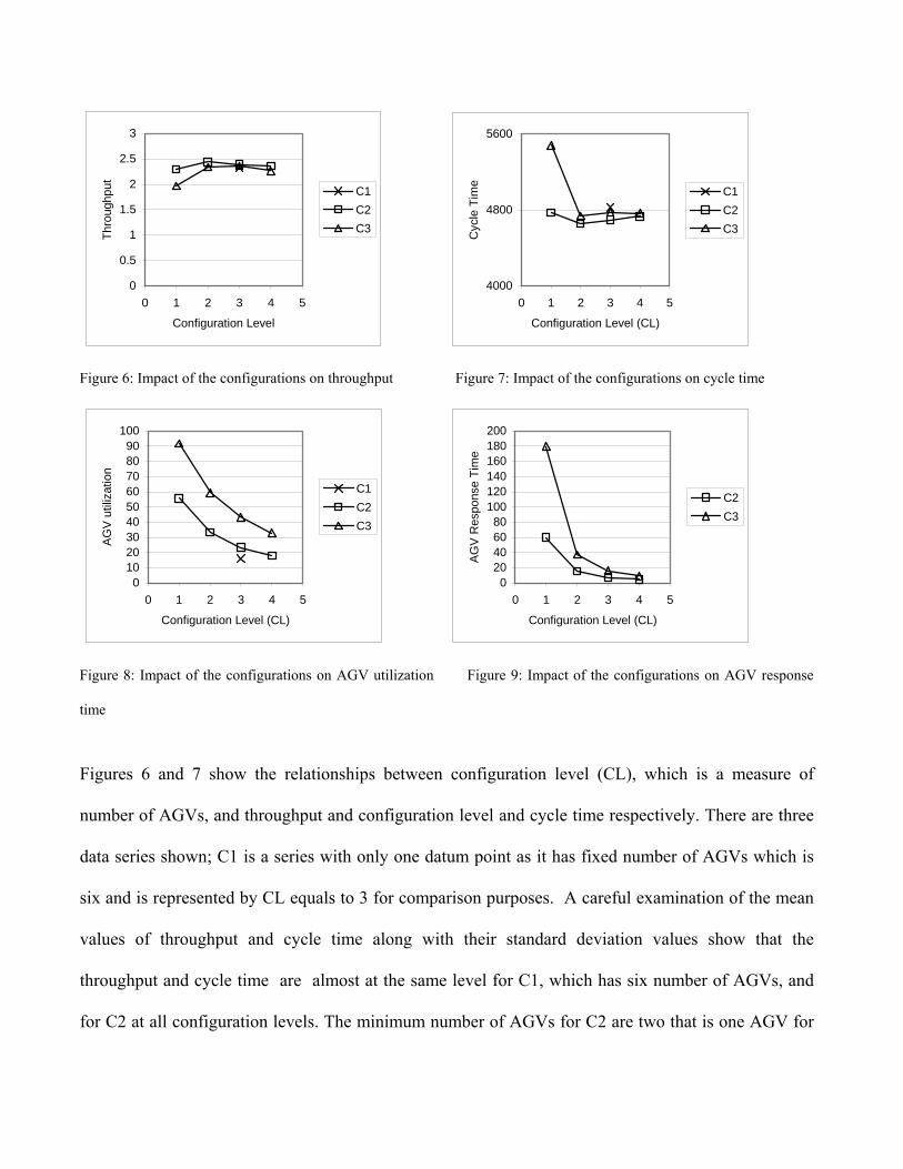
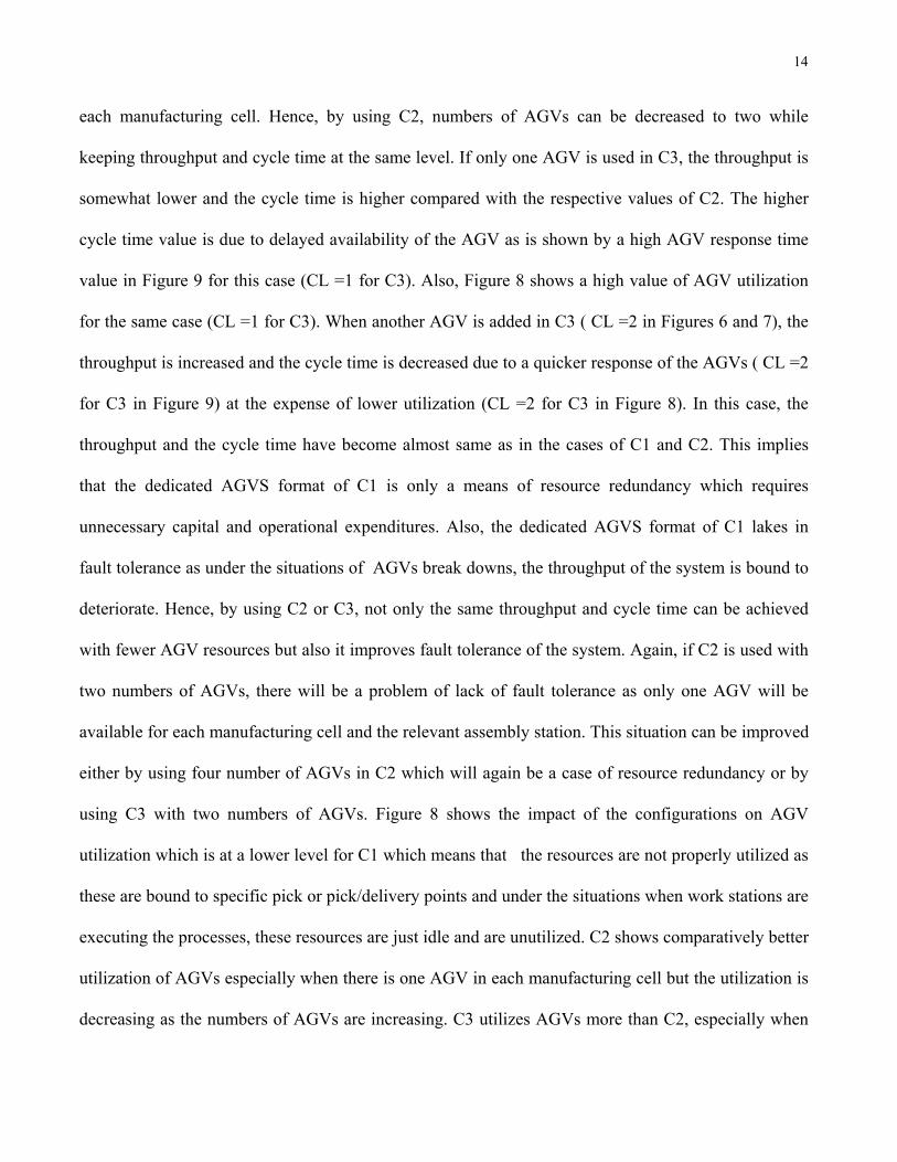
Figure 6: Impact of the configurations on throughput Figure 7: Impact of the configurations on cycle time

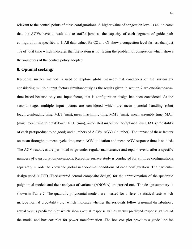
0102030405060708090

100

0 1 2 3 4 5

Configuration Level (CL)

AG

V u

tiliz

atio

n

C1C2C3

020406080

100120140160180200

0 1 2 3 4 5

Configuration Level (CL)

AG

V R

espo

nse

Tim

e

C2C3

Figure 8: Impact of the configurations on AGV utilization Figure 9: Impact of the configurations on AGV response

time

Figures 6 and 7 show the relationships between configuration level (CL), which is a measure of

number of AGVs, and throughput and configuration level and cycle time respectively. There are three

data series shown; C1 is a series with only one datum point as it has fixed number of AGVs which is

six and is represented by CL equals to 3 for comparison purposes. A careful examination of the mean

values of throughput and cycle time along with their standard deviation values show that the

throughput and cycle time are almost at the same level for C1, which has six number of AGVs, and

for C2 at all configuration levels. The minimum number of AGVs for C2 are two that is one AGV for

14

each manufacturing cell. Hence, by using C2, numbers of AGVs can be decreased to two while

keeping throughput and cycle time at the same level. If only one AGV is used in C3, the throughput is

somewhat lower and the cycle time is higher compared with the respective values of C2. The higher

cycle time value is due to delayed availability of the AGV as is shown by a high AGV response time

value in Figure 9 for this case (CL =1 for C3). Also, Figure 8 shows a high value of AGV utilization

for the same case (CL =1 for C3). When another AGV is added in C3 ( CL =2 in Figures 6 and 7), the

throughput is increased and the cycle time is decreased due to a quicker response of the AGVs ( CL =2

for C3 in Figure 9) at the expense of lower utilization (CL =2 for C3 in Figure 8). In this case, the

throughput and the cycle time have become almost same as in the cases of C1 and C2. This implies

that the dedicated AGVS format of C1 is only a means of resource redundancy which requires

unnecessary capital and operational expenditures. Also, the dedicated AGVS format of C1 lakes in

fault tolerance as under the situations of AGVs break downs, the throughput of the system is bound to

deteriorate. Hence, by using C2 or C3, not only the same throughput and cycle time can be achieved

with fewer AGV resources but also it improves fault tolerance of the system. Again, if C2 is used with

two numbers of AGVs, there will be a problem of lack of fault tolerance as only one AGV will be

available for each manufacturing cell and the relevant assembly station. This situation can be improved

either by using four number of AGVs in C2 which will again be a case of resource redundancy or by

using C3 with two numbers of AGVs. Figure 8 shows the impact of the configurations on AGV

utilization which is at a lower level for C1 which means that the resources are not properly utilized as

these are bound to specific pick or pick/delivery points and under the situations when work stations are

executing the processes, these resources are just idle and are unutilized. C2 shows comparatively better

utilization of AGVs especially when there is one AGV in each manufacturing cell but the utilization is

decreasing as the numbers of AGVs are increasing. C3 utilizes AGVs more than C2, especially when

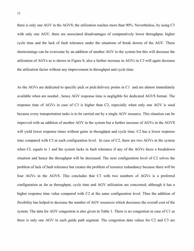
15

there is only one AGV in the AGVS; the utilization reaches more than 90%. Nevertheless, by using C3

with only one AGV, there are associated disadvantages of comparatively lower throughput, higher

cycle time and the lack of fault tolerance under the situations of break downs of the AGV. These

shortcomings can be overcome by an addition of another AGV to the system but this will decrease the

utilization of AGVs as is shown in Figure 8; also a further increase in AGVs in C3 will again decrease

the utilization factor without any improvement in throughput and cycle time.

As the AGVs are dedicated to specific pick or pick/delivery points in C1 and are almost immediately

available when are needed , hence AGV response time is negligible for dedicated AGVS format. The

response time of AGVs in case of C3 is higher than C2, especially when only one AGV is used

because every transportation tasks is to be carried out by a single AGV resource. This situation can be

improved with an addition of another AGV in the system but a further increase of AGVs in the AGVS

will yield lower response times without gains in throughput and cycle time. C2 has a lower response

time compared with C3 at each configuration level. In case of C2, there are two AGVs in the system

when CL equals to 1 and the system lacks in fault tolerance if any of the AGVs faces a breakdown

situation and hence the throughput will be decreased. The next configuration level of C2 solves the

problem of lack of fault tolerance but creates the problem of resource redundancy because there will be

four AGVs in the AGVS. This concludes that C3 with two numbers of AGVs is a preferred

configuration as far as throughput, cycle time and AGV utilization are concerned; although it has a

higher response time value compared with C2 at the same configuration level. Thus the addition of

flexibility has helped to decrease the number of AGV resources which decreases the overall cost of the

system. The data for AGV congestion is also given in Table 1. There is no congestion in case of C1 as

there is only one AGV in each guide path segment. The congestion data values for C2 and C3 are

16

relevant to the control points of these configurations. A higher value of congestion level is an indicator

that the AGVs have to wait due to traffic jams as the capacity of each segment of guide path

configuration is specified to 1. All data values for C2 and C3 show a congestion level far less than just

1% of total time which indicates that the system is not facing the problem of congestion which shows

the soundness of the control policy adopted.

8. Optimal seeking:

Response surface method is used to explore global near-optimal conditions of the system by

considering multiple input factors simultaneously as the results given in section 7 are one-factor-at-a-

time based because only one input factor, that is configuration design has been considered. At the

second stage, multiple input factors are considered which are mean material handling robot

loading/unloading time, MLT (min), mean machining time, MMT (min), mean assembly time, MAT

(min), mean time to breakdown, MTB (min), automated inspection acceptance level, IAL (probability

of each part/product to be good) and numbers of AGVs, AGVs ( number). The impact of these factors

on mean throughput, mean cycle time, mean AGV utilization and mean AGV response time is studied.

The AGV resources are permitted to go under regular maintenance and repairs events after a specific

numbers of transportation operations. Response surface study is conducted for all three configurations

separately in order to know the global near-optimal conditions of each configuration. The particular

design used is FCD (Face-centred central composite design) for the approximation of the quadratic

polynomial models and their analyses of variance (ANOVA) are carried out. The design summary is

shown in Table 2. The quadratic polynomial models are tested for different statistical tests which

include normal probability plot which indicates whether the residuals follow a normal distribution ,

actual versus predicted plot which shows actual response values versus predicted response values of

the model and box cox plot for power transformation. The box cox plot provides a guide line for

17

selecting the correct power law transformation. The transformation of a response is recommended

based on the best transformation power value found at the minimum point of the curve generated by

the natural log of the sum of squares of residuals. Due to space limitation, the details of these tests are

not shown here. The quadratic polynomial modelling for mean throughput, mean cycle time and mean

AGV utilization for configuration 1 is given. Similarly, the models have been developed for

configurations 2 and 3 but are not shown here due to space limitation. The output responses can vary

from the most ( taken as 5) to the least ( taken as 1) important responses. For optimization, throughput

and cycle time are considered more important responses whereas other responses are taken as less

important. Table 2 also gives constraints for optimization. The following are the polynomial models

for C1.

Log10( Mean Throughput) = +0.10485 - 0.025058 * MLT- 0.16219 * MMT - 0.15981 * MAT +

0.11782 * MTB +10.11561 * IAL+ 0.015762 * MLT * MMT + 0.016294 *

MLT * MAT +2.83738E-004 * MLT * MTB - 0.69827 * MLT * IAL

+0.016368 * MMT * MAT -5.31516E-004 * MMT * MTB +0.24977 *

MMT * IAL +3.35754E-003 * MAT * MTB +0.30651 * MAT * IAL -

0.046493 * MTB * IAL -0.011028 * MLT2 -9.14639E-003 * MMT2 -

1.85258E-003 * MAT2 -5.55070E-003 * MTB2 -32.13320 * IAL2

Log10(Mean Cycle Time) = +3.83908+0.035853 * MLT+0.088559 * MMT+0.17880 * MAT-

0.099430 * MTB -8.47121 * IAL-0.012753 * MLT * MMT-0.017724 *

MLT * MAT+3.14536E-004 * MLT * MTB + 0.64231 * MLT * IAL -

0.018805 * MMT * MAT+3.13813E-003 * MMT * MTB +0.074282 *

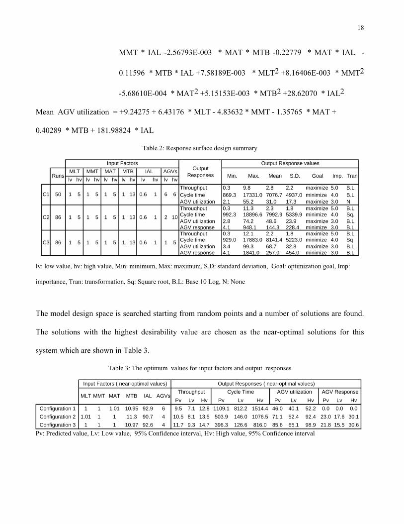
18

MMT * IAL -2.56793E-003 * MAT * MTB -0.22779 * MAT * IAL -

0.11596 * MTB * IAL +7.58189E-003 * MLT2 +8.16406E-003 * MMT2

-5.68610E-004 * MAT2 +5.15153E-003 * MTB2 +28.62070 * IAL2

Mean AGV utilization = +9.24275 + 6.43176 * MLT - 4.83632 * MMT - 1.35765 * MAT +

0.40289 * MTB + 181.98824 * IAL

Table 2: Response surface design summary

lv hv lv hv lv hv lv hv lv hv lv hvThroughput 0.3 9.8 2.8 2.2 maximize 5.0 B.LCycle time 869.3 17331.0 7076.7 4937.0 minimize 4.0 B.LAGV utilization 2.1 55.2 31.0 17.3 maximize 3.0 NThroughput 0.3 11.3 2.3 1.8 maximize 5.0 B.LCycle time 992.3 18896.6 7992.9 5339.9 minimize 4.0 Sq.AGV utilization 2.8 74.2 48.6 23.9 maximize 3.0 B.LAGV response 4.1 948.1 144.3 228.4 minimize 3.0 B.LThroughput 0.3 12.1 2.2 1.8 maximize 5.0 B.LCycle time 929.0 17883.0 8141.4 5223.0 minimize 4.0 SqAGV utilization 3.4 99.3 68.7 32.8 maximize 3.0 B.LAGV response 4.1 1841.0 257.0 454.0 minimize 3.0 B.L

Runs

Output Response valuesOutput

Responses

1 5

102

1 5 1 5 1 5 1 13 0.6

13 0.6 1

1

1 6 6

1 5 1 5 1 5 1

1 5 1 5 1 5 1 13 0.6

Input FactorsMLT MMT MAT MTB IAL AGVs

50

86

86

C1

C2

C3

Goal Imp. TranMin. Max. Mean S.D.

lv: low value, hv: high value, Min: minimum, Max: maximum, S.D: standard deviation, Goal: optimization goal, Imp:

importance, Tran: transformation, Sq: Square root, B.L: Base 10 Log, N: None

The model design space is searched starting from random points and a number of solutions are found.

The solutions with the highest desirability value are chosen as the near-optimal solutions for this

system which are shown in Table 3.

Table 3: The optimum values for input factors and output responses

Pv Lv Hv Pv Lv Hv Pv Lv Hv Pv Lv HvConfiguration 1 1 1 1.01 10.95 92.9 6 9.5 7.1 12.8 1109.1 812.2 1514.4 46.0 40.1 52.2 0.0 0.0 0.0Configuration 2 1.01 1 1 11.3 90.7 4 10.5 8.1 13.5 503.9 146.0 1076.5 71.1 52.4 92.4 23.0 17.6 30.1Configuration 3 1 1 1 10.97 92.6 4 11.7 9.3 14.7 396.3 126.6 816.0 85.6 65.1 98.9 21.8 15.5 30.6

AGVsMMT MAT MTB IALAGV Response

Input Factors ( near-optimal values) Output Responses ( near-optimal values)Throughput Cycle Time AGV utilization

MLT

Pv: Predicted value, Lv: Low value, 95% Confidence interval, Hv: High value, 95% Confidence interval

Figure 10 gives a performance comparison for all three configurations. The throughput has been

increased and the cycle time has been decreased gradually as we move from C1 towards C3. The

increase in throughput from C1 to C3 is around 23% and the decrease in cycle time is around 64 %.

The AGV utilization has been increased approximately 86% from C1 to C3 where as AGV response

has shown a small decrease from C2 to C3. For each configuration, the near-optimal output responses

are achieved along with the near-optimal conditions of input factors. MLT, MMT and MAT are found

at either their minimum or close to minimum values as the higher these values are, the longer will be

the cycle time and the lower will be the throughput values. The values of MTB are considerably higher

than MLT, MMT and MAT in order to have a lower probability of resource breakdown during process

execution and the values of IAL are higher to impose a very low probability of rejection of any part/

material at automated inspection.

C1

C1

C1

C2

C2

C2

C2

C3

C3

C3

C3

1

10

100

1000

10000

Throug

hput

Cycle

Time

AGV utiliz

ation

AGV Res

pons

e

Out

put R

espo

nse

valu

e ( L

ogrit

hmic

sca

le)

C1C2C3

Figure 10: Comparison of all Responses for three configurations.

20

9. Conclusion:

This study has attempted to apply advanced tools of coloured Petri net and response surface methods

to model and analyze the practical constraints of an integrated automated guided vehicle system. The

flexibility addition in terms of guide path design to accommodate varying number of AGVs has led to

identify redundant AGV resources in dedicated AGVS format which can be removed and hence the

overall cost of the system can be decreased while keeping the throughput and cycle time of the system

at the same level. The fault tolerance of the system has also improved through the introduction of

guide path flexibility. Also, it has attempted to find global near-optimal solution of multiple responses

simultaneously through desirability function approach. The mean throughput and mean cycle time has

been considered more important output responses. The throughput, cycle time and AGV utilization

have shown gradual improvement along with a decrease in the numbers of AGV resources subject to

optimization constraints as the AGVS guide path flexibility is enhanced. The DEDS modelling,

analysis and optimization approach based on CPM and RSM can be used as a general methodology for

achieving the best performance of a DEDS.

References

[1] A.A. Desrochers, and R.Y. Al-Jaar, Applications of petri nets in manufacturing Systems: Modeling,

Control and performance Analysis, IEEE Press 1995.

[2] F. Tamer, Abdelmaguid, O. N. Ashraf, A. B. Kamal and M.F. Hassan, “A hybrid GA/heuristic

approach to the simultaneous scheduling of machines and automated guided vehicles” Int.J.Prod.Res.,

2004, Vol.42-2, 267-281.

[3] G.Ulusoy and U.Bilge, “Simultaneous Scheduling of machines and automated guided vehicles”

Int.J.Prod.Res. 1993, Vol.31-2, 2857-2873.

21

[4] N. Jawahar, P. Aravindan, S.G. Ponnambalam and R.K. Suresh, “AGV Schedule Integrated with

Production in Flexible Manufacturing Systems” Int. J. Adv. Manuf. Technol (1998) 14: 428-440.

[5] Y. Seo and P. J Egbelu, “Integrated manufacturing planning for an AGV-based FMS”

Int.J.Prod.Econ. 60-61 (1999) 473-478.

[6] I. F. A. Vis, “Survey of research in the design and control of automated guided vehicle systems”

European Journal of Operational Research 170 (2006) 677-709.

[7] T. Le-Anh and M. B. M De Koster, “A review of design and control of automated guided vehicle

systems” European Journal of Operational Research, 171-1 (2006), pp. 1-23.

[8] R.J. Gaskins and J. M. A. Tanchoco, “Flow path design for automated guided vehicle systems”

Int.J.Prod.Res. 25(5), 1987, pp. 667-676.

[9] M. Kaspi and J. M. A. Tanchoco, “Optimal flow path design of unidirectional AGV system”

Int.J.Prod.Res. 28(6), 1990, pp. 1023-1030.

[10] S. Rajotia, K. Shankar and J. L. Batra, “An heuristic for configuring a mixed uni/bidirectional

flow path for an AGV System” Int.J.Prod.Res. 36(7), 1998, pp. 1779-1799.

[11] B. E. Farling, C. T. Mosier and F. Mahmood, “Analysis of automated guided vehicle

configurations in flexible manufacturing systems” Int.J.Prod.Res. 2001, 39(18), pp. 4239-4260.

[12] K. Jensen, Coloured Petri Nets: Basic Concepts, Analysis Methods and Practical Use, V. 1,

Springer – Verlag, 1992.

[13] T. Aized, K. Takahashi, I. Hagiwara, “ Advanced Multiple-Product Manufacturing System

Modelling using Coloured Petri Net” Proc. SCIS & ISIS 2006, Tokyo, Sep. 20-24 2006, pp. 2075-

2080.

22

[14] T. Aized, K. Takahashi, I. Hagiwara, “The Modelling and analysis of Guide-path configurations

of an integrated Automated guided Vehicle System using Coloured Petri Net” IEICE Technical Report

CST2006-38 ( 2007-01).

[15 M. J. Anderson and P. J. Whitcomb, RSM simplified, productivity press, NY, 2005.

[16] G. Derringer and R. Suich, “Simultaneous optimization of several response variables” Journal of

quality technology, 12, pp. 214-219, 1980.

[17] S. Robinson, “A statistical process control approach for estimating the warm-up period” Proc.

winter simulation conference, pp. 439-445, 2002.