Int J Adv Manuf Technol (2017) 92:1825–1837DOI 10.1007/s00170-017-0175-7

ORIGINAL ARTICLE

Automated guided vehicle mission reliability modellingusing a combined fault tree and Petri net approach

Rundong Yan1 · Lisa M. Jackson1 · Sarah J. Dunnett1

Received: 30 November 2016 / Accepted: 16 February 2017 / Published online: 21 March 2017© The Author(s) 2017. This article is published with open access at Springerlink.com

Abstract Automated guided vehicles (AGVs) are beingextensively used for intelligent transportation and distribu-tion of materials in warehouses and autoproduction linesdue to their attributes of high efficiency and low costs.Such vehicles travel along a predefined route to deliverdesired tasks without the supervision of an operator. Mucheffort in this area has focused primarily on route optimisa-tion and traffic management of these AGVs. However, thehealth management of these vehicles and their optimal mis-sion configuration have received little attention. To assuretheir added value, taking a typical AGV transport systemas an example, the capability to evaluate reliability issuesin AGVs are investigated in this paper. Following a fail-ure modes effects and criticality analysis (FMECA), thereliability of the AGV system is analysed via fault tree anal-ysis (FTA) and the vehicles mission reliability is evaluatedusing the Petri net (PN) method. By performing the analysis,the acceptability of failure of the mission can be analysed,and hence the service capability and potential profit of theAGV system can be reviewed and the mission altered whereperformance is unacceptable. The PN method could easilybe extended to have the capability to deal with fleet AGVmission reliability assessment.

� Rundong Yanr.yan@lboro.ac.uk

Lisa M. Jacksonl.m.jackson@lboro.ac.uk

Sarah J. Dunnetts.j.dunnett@lboro.ac.uk

1 Loughborough University, Loughborough, Leicestershire,LE11 3TU, UK

Keywords Automated guided vehicles · Reliability · Petrinets · Fault tree analysis

1 Introduction

For intelligent transportation and distribution of materials inwarehouses and/or manufacturing facilities, there has beenin recent years the increasing use of automated guided vehi-cles (AGVs). Such vehicles travel along predefined routesto deliver various tasks without the supervision of an on-board operator. As the AGV systems are getting larger andmore complex, increasing the efficiency and lowering theoperation cost of the AGV system have naturally becomethe first priorities, via investigating the design and controlaspects of the AGV [1–4], by identifying new flow-pathlayouts including workstation layouts [5–7] and developingadvanced traffic management strategies, including vehiclerouting and task assignment [8–13]. Trenkle [14] introducedthe safety requirements and safety functions for a decen-tralised controlled AGV system. Three major hazards, i.e.collision with a person, tilting over and falling down, wereidentified. The effects of the speed of AGVs, the brakingdistance and detection area requirements as well as the meantime to dangerous failure and performance were analysed.Regarding failure response, Ebben developed a method forfailure control management for a special case study ofAGVs, an underground transportation system (with loadedand unloaded AGVs considered) [15]. In the area of thereliability modelling of AGVs, Fazlollahtabar [16] createda model to maximise the reliability of AGVs and minimisetheir repair cost, and Tavana and Fazlollahtabar modelledthe reliability of AGVs as a cost function to optimise timeand cost objectives [17]. However, fully understanding howAGVs can fail and the causes of such failures is still needed.

1826 Int J Adv Manuf Technol (2017) 92:1825–1837

Some progress was made in this area by Duran et al.[18] who attempted to identify the basic failure modes ofthe light detection and ranging (LIDAR) system and thecamera-based computer vision system (CV) on AGVs byusing a combined approach of fault tree analysis (FTA) andBayesian belief networks (BN). In the work, human injury,property damage and vehicle damage were defined as thetop events in the fault tree. However, the research did notcover all components and subassemblies included in AGVs.

Modelling using Petri net (PN) has been becoming acommon tool and popular research topic to evaluate reliabil-ity of a system or a mission. For example, Wu proposed anextended object-oriented Petri net model to analyse the reli-ability of a phased mission with common cause failures in2015. [19] On the other hand, from the aspect of industrialapplications, Le and Andrews [20] presented a wind tur-bine asset model to study the degradation, maintenance andinspection processes of different wing tunnel componentsbased on PNs. However, to date the Petri net (PN) methodhas only been used as a mathematical tool to investigateroute planning and control strategies for AGV systems. Forexample, Luo and Ni [21] designed a programmable logi-cal controller (PLC) using Petri nets to prevent collisionsof vehicles in an AGV system and Nishi and Maeno [22]proposed an approach to optimise the routing planning forAGVs in semiconductor fabrication bays.

However, to the best of the authors knowledge, PNs haverarely been applied to the study of the reliability of AGVs.In particular, their application to mission reliability. This isthe aim of the work presented in this paper. In contrast tothe combined approach of FTA and BN adopted in [18], thecombined use of FTA and PNs adopted here enables notonly the analysis of all failure modes of all the subsystemsbut also an analysis of the mission of the AGV . In addition,the PNs can be easily modified if the mission changed.

In a system with only a few AGVs, the failure of any oneof the AGVs will not cause a significant traffic congestionissue. Moreover, the failed AGV can be quickly replacedby back up ones. Hence, such a small scale AGV applica-tion system can be easily managed [1]. However, given theincreasing number of large scale AGV application systemswhere a significant number of AGVs share the limited num-ber of travel routes, the failure of any one of these AGVswill cause serious traffic chaos. Hence, for this reason, con-sidering a complete investigation of the reliability issues ofall AGV components and subassemblies is important notonly to ensure the high reliability and availability of AGVsand their success of delivering prescribed tasks but also tooptimise their maintenance strategies and minimise trafficchaos. The reliability issues of the whole AGV system areinvestigated through assessing the reliability of a typicalAGV transport system in this paper, where the capability toconsider mission analysis of AGVs is shown. The novelties

of this paper can be summarise as the following: an effectivereliability assessment of AGVs using combined FTA andPNs has been proposed. Using the techniques developed,the critical phases in the AGV mission can be identified andtheir failure probability can be obtained. The PN simulationis found to be an efficient and adaptable method to analysethe reliability of complex AGV systems undertaking varioustasks.

The remaining part of the paper is organised as follows.In Section 2, the reliability modelling methods are discussedwith the AGV application system being the focus of Section3. Section 4 covers the AGV system reliability model gener-ation and the AGV mission analysis is covered in Section 5.The simulation method adopted and the results are presentedin Section 6 with the conclusions in the final section.

2 Reliability modelling

One of the most commonly used reliability methods, widelyadopted in industrial practise, is fault tree analysis (FTA).This method allows a system failure mode to be expressedin terms of the interactions of its components. Moreover,with the aid of FTA, the probability of system or missionfailure can be computed via Boolean logic calculations. Thismethod has been adopted to evaluate the subsystem levelfailures for the AGV system.

When the system is large and complex, or the missionperformed is made up of many phases, FTA can becomeinaccurate and computationally expensive. In such cases,alternative reliability modelling methods may be bettersuited to performance analysis, one such technique beingPetri nets (PNs), developed by Petri [23]. Similar to FTA,PNs provide an intuitive graphical representation of the sys-tem being modelled allowing for reliability investigation.The PN method is a direct bipartite graph which consists offour types of symbol: circles, rectangles, arrows and tokens.Circles represent the places, which are conditions or statessuch as mission failure, phase failure or component failure;rectangles represent the transitions, more abstractly actionsor events which cause the change of condition or state. Itshould be mentioned that if the time for completing the tran-sition is zero, the rectangle is filled in, otherwise it is hollow;arrows represent arcs which are connections between placesand transitions. Arcs with a slash on and a number, n, nextto the slash represent a combination of n single arcs and thearc is said to have a weight n. No slash always means thatthe weight is one; and small filled in circles represent tokenswhich carry the information in the PNs. The tokens movevia transitions as long as the enabling condition explainedbelow is satisfied, which gives the dynamic properties of thePNs. The marking of a net at any particular time gives thestate of the system being modelled at that time.

Int J Adv Manuf Technol (2017) 92:1825–1837 1827

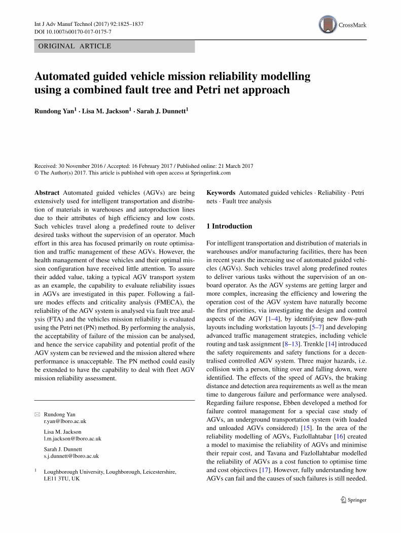
Figure 1 shows an example net where movement oftokens have occurred after a time period, hence the tokensmake a transition through the net. The net has two inputplaces (represented by circles) and one output place (drawnas a circle) connected by a timed transition (hollow rectan-gle) with a time delay t. There is one token and three tokens(represented by small filled in circles) in each of the twoinput places. The input places have arcs with weights 1 and2, respectively. Currently, there are no tokens in the outputplace; however, a transition will be enabled when the num-ber of tokens contained in every input place is equal to ormore than the corresponding arc weights. Given this is truefor the net shown in Fig. 1, the transition is enabled and thenumber of tokens equivalent to the output arc number aretransferred to the output place; in this instance, one tokenappears in the output place. The number of tokens movedto the output place is dependent on the corresponding arcweight, hence if the arc weight is ‘n’, then n more tokenswill appear in the output place after the transition fires.

Petri nets for system representations are built up usingthese same components. Research has shown the applica-tion of these nets to systems that undertake phased missions,where a net is generated for the system and an additionalnet is developed for the phase, known as a system and phasenet, respectively [24]. Extensions for more complex sys-tems have included using three distinct PNs, i.e. phase PN,component PN and master PN [25]. These three kinds ofPNs are linked together and interact with each other. Suchan extended approach is adopted in this paper to assess thereliability of AGV systems.

3 Application AGV system and mission

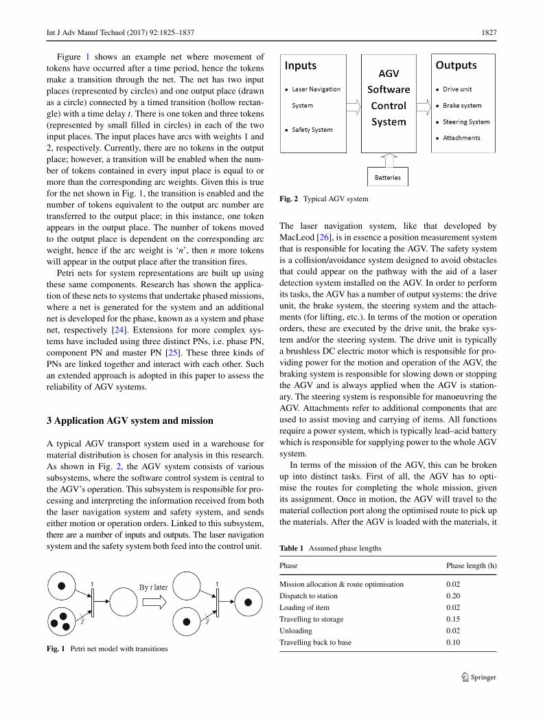
A typical AGV transport system used in a warehouse formaterial distribution is chosen for analysis in this research.As shown in Fig. 2, the AGV system consists of varioussubsystems, where the software control system is central tothe AGV’s operation. This subsystem is responsible for pro-cessing and interpreting the information received from boththe laser navigation system and safety system, and sendseither motion or operation orders. Linked to this subsystem,there are a number of inputs and outputs. The laser navigationsystem and the safety system both feed into the control unit.

Fig. 1 Petri net model with transitions

Fig. 2 Typical AGV system

The laser navigation system, like that developed byMacLeod [26], is in essence a position measurement systemthat is responsible for locating the AGV. The safety systemis a collision/avoidance system designed to avoid obstaclesthat could appear on the pathway with the aid of a laserdetection system installed on the AGV. In order to performits tasks, the AGV has a number of output systems: the driveunit, the brake system, the steering system and the attach-ments (for lifting, etc.). In terms of the motion or operationorders, these are executed by the drive unit, the brake sys-tem and/or the steering system. The drive unit is typicallya brushless DC electric motor which is responsible for pro-viding power for the motion and operation of the AGV, thebraking system is responsible for slowing down or stoppingthe AGV and is always applied when the AGV is station-ary. The steering system is responsible for manoeuvring theAGV. Attachments refer to additional components that areused to assist moving and carrying of items. All functionsrequire a power system, which is typically lead–acid batterywhich is responsible for supplying power to the whole AGVsystem.

In terms of the mission of the AGV, this can be brokenup into distinct tasks. First of all, the AGV has to opti-mise the routes for completing the whole mission, givenits assignment. Once in motion, the AGV will travel to thematerial collection port along the optimised route to pick upthe materials. After the AGV is loaded with the materials, it

Table 1 Assumed phase lengths

Phase Phase length (h)

Mission allocation & route optimisation 0.02

Dispatch to station 0.20

Loading of item 0.02

Travelling to storage 0.15

Unloading 0.02

Travelling back to base 0.10

1828 Int J Adv Manuf Technol (2017) 92:1825–1837

will travel to the destination and unload the materials. Aftersuccessfully distributing the materials, the AGV will travelback to its original parking position. Therefore, the wholemission can be divided into six phases in total, namely (1)mission allocation and route optimisation, (2) dispatch tostation, (3) loading of item, (4) travelling to storage, (5)unloading and (6) travelling back to base. The mission canbe regarded as successful only when the AGV is able tooperate successfully throughout all these six phases withoutany break due to component and/or subsystem failures andmaintenance. Such a period is named as a maintenance-freeoperational period (MFOP) [27].

In order to calculate the phase mission reliability, thelength of each phase (i.e. the time duration for completingeach phase) is required and the values assumed in this workare shown in Table 1. These values taken are for demon-stration purposes, where the total time duration to completethe whole mission is 0.51 h. It is worth mentioning that theassumed values in Table 1 are based on the consultation withan AGV operator. These values would be different for differentapplications. Therefore, the time duration should be modifiedcorrespondingly when considering different AGV applications.

4 AGV reliability model generation

4.1 Subsystem level reliability models

Initially, a detailed FMECA analysis of the AGV (with anextract illustrated in Table 2) was performed in order toobtain a detailed understanding of the vehicle. Eight subsys-tems were identified for analysis. In Table 2, the subsystem,the laser navigation system (LNS), is shown where columnslabelled S, F, D and RPN refer to the severity ranking,frequency ranking, detectability ranking (all with ratings1–5) and risk priority number, respectively (calculated as

the multiplicity of all three rankings). Similar tables weredeveloped for all AGV subsystems.

The understanding gained from the FMECA was then usedto construct fault trees describing the failure of each subsystem.

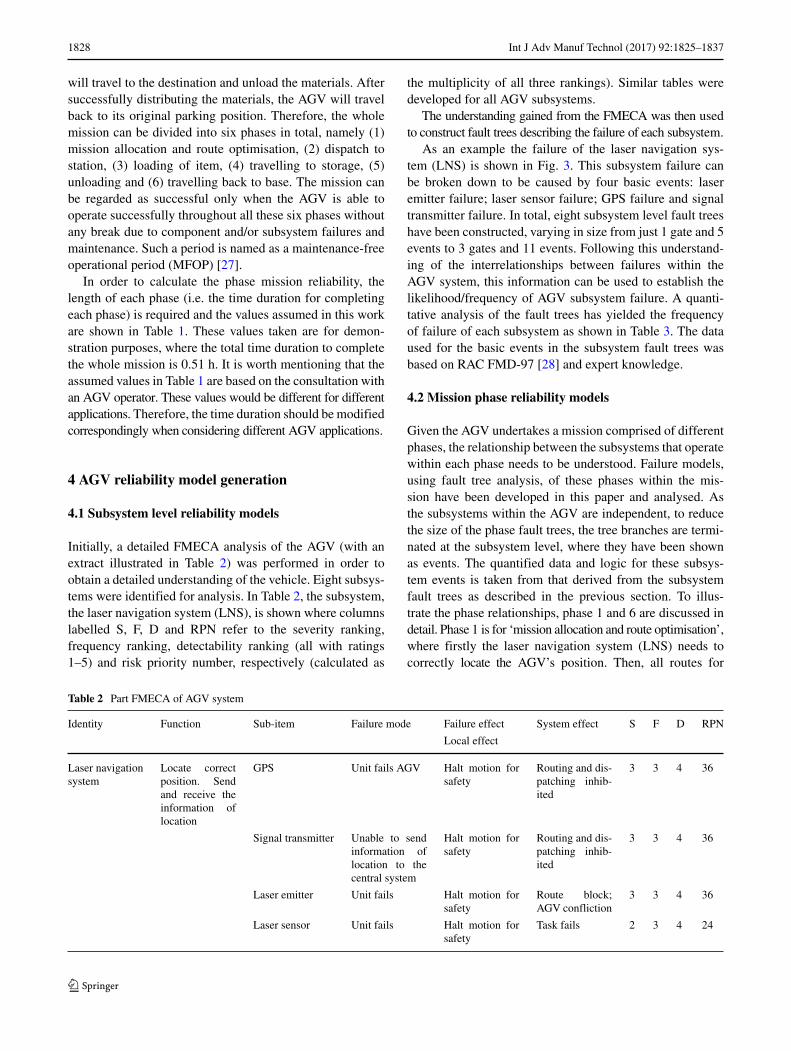
As an example the failure of the laser navigation sys-tem (LNS) is shown in Fig. 3. This subsystem failure canbe broken down to be caused by four basic events: laseremitter failure; laser sensor failure; GPS failure and signaltransmitter failure. In total, eight subsystem level fault treeshave been constructed, varying in size from just 1 gate and 5events to 3 gates and 11 events. Following this understand-ing of the interrelationships between failures within theAGV system, this information can be used to establish thelikelihood/frequency of AGV subsystem failure. A quanti-tative analysis of the fault trees has yielded the frequencyof failure of each subsystem as shown in Table 3. The dataused for the basic events in the subsystem fault trees wasbased on RAC FMD-97 [28] and expert knowledge.

4.2 Mission phase reliability models

Given the AGV undertakes a mission comprised of differentphases, the relationship between the subsystems that operatewithin each phase needs to be understood. Failure models,using fault tree analysis, of these phases within the mis-sion have been developed in this paper and analysed. Asthe subsystems within the AGV are independent, to reducethe size of the phase fault trees, the tree branches are termi-nated at the subsystem level, where they have been shownas events. The quantified data and logic for these subsys-tem events is taken from that derived from the subsystemfault trees as described in the previous section. To illus-trate the phase relationships, phase 1 and 6 are discussed indetail. Phase 1 is for ‘mission allocation and route optimisation’,where firstly the laser navigation system (LNS) needs tocorrectly locate the AGV’s position. Then, all routes for

Table 2 Part FMECA of AGV system

Identity Function Sub-item Failure mode Failure effect System effect S F D RPN

Local effect

Laser navigationsystem

Locate correctposition. Sendand receive theinformation oflocation

GPS Unit fails AGV Halt motion forsafety

Routing and dis-patching inhib-ited

3 3 4 36

Signal transmitter Unable to sendinformation oflocation to thecentral system

Halt motion forsafety

Routing and dis-patching inhib-ited

3 3 4 36

Laser emitter Unit fails Halt motion forsafety

Route block;AGV confliction

3 3 4 36

Laser sensor Unit fails Halt motion forsafety

Task fails 2 3 4 24

Int J Adv Manuf Technol (2017) 92:1825–1837 1829

Laser Navigation

System Failures

LNS Fails to

obtain Accurate

Location

Signal

Transmitter Fails

Laser Part

fails

GPS Fails to Obtain

Approximate Location

Laser Emitter

Fails

Laser Sensor

Fails

SensorEmitter

GPS

Trans

Fig. 3 Laser navigation subsystem level fault tree

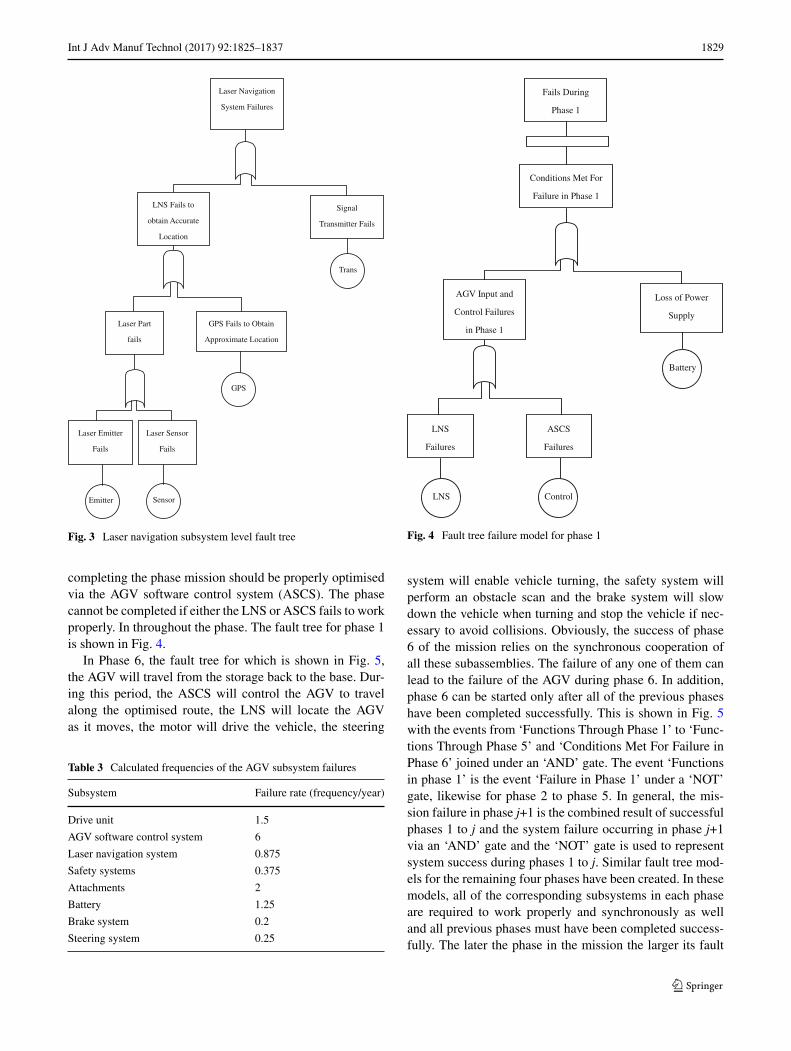
completing the phase mission should be properly optimisedvia the AGV software control system (ASCS). The phasecannot be completed if either the LNS or ASCS fails to workproperly. In throughout the phase. The fault tree for phase 1is shown in Fig. 4.

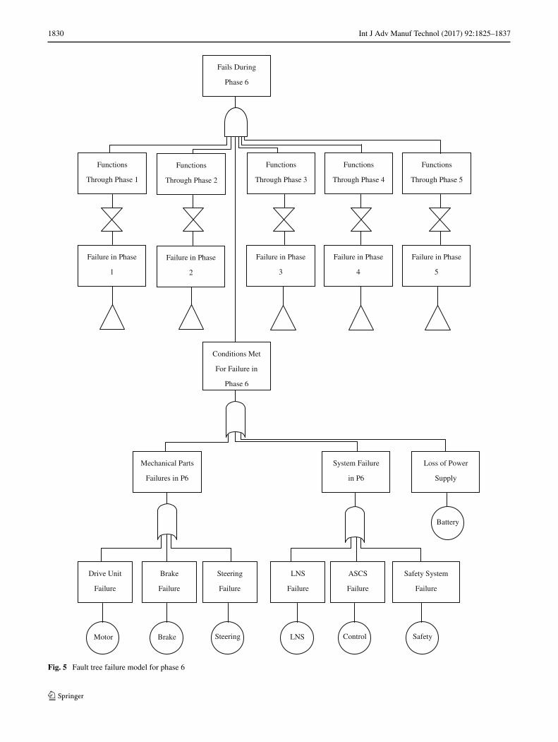
In Phase 6, the fault tree for which is shown in Fig. 5,the AGV will travel from the storage back to the base. Dur-ing this period, the ASCS will control the AGV to travelalong the optimised route, the LNS will locate the AGVas it moves, the motor will drive the vehicle, the steering

Table 3 Calculated frequencies of the AGV subsystem failures

Subsystem Failure rate (frequency/year)

Drive unit 1.5

AGV software control system 6

Laser navigation system 0.875

Safety systems 0.375

Attachments 2

Battery 1.25

Brake system 0.2

Steering system 0.25

Conditions Met For

Failure in Phase 1

AGV Input and

Control Failures

in Phase 1

Loss of Power

Supply

LNS

Failures

ASCS

Failures

Control

Battery

LNS

Fails During

Phase 1

Fig. 4 Fault tree failure model for phase 1

system will enable vehicle turning, the safety system willperform an obstacle scan and the brake system will slowdown the vehicle when turning and stop the vehicle if nec-essary to avoid collisions. Obviously, the success of phase6 of the mission relies on the synchronous cooperation ofall these subassemblies. The failure of any one of them canlead to the failure of the AGV during phase 6. In addition,phase 6 can be started only after all of the previous phaseshave been completed successfully. This is shown in Fig. 5with the events from ‘Functions Through Phase 1’ to ‘Func-tions Through Phase 5’ and ‘Conditions Met For Failure inPhase 6’ joined under an ‘AND’ gate. The event ‘Functionsin phase 1’ is the event ‘Failure in Phase 1’ under a ‘NOT’gate, likewise for phase 2 to phase 5. In general, the mis-sion failure in phase j+1 is the combined result of successfulphases 1 to j and the system failure occurring in phase j+1via an ‘AND’ gate and the ‘NOT’ gate is used to representsystem success during phases 1 to j. Similar fault tree mod-els for the remaining four phases have been created. In thesemodels, all of the corresponding subsystems in each phaseare required to work properly and synchronously as welland all previous phases must have been completed success-fully. The later the phase in the mission the larger its fault

1830 Int J Adv Manuf Technol (2017) 92:1825–1837

Fails During

Phase 6

Functions

Through Phase 1

Functions

Through Phase 2

Functions

Through Phase 3

Functions

Through Phase 4

Functions

Through Phase 5

Failure in Phase

1

Failure in Phase

2

Failure in Phase

3

Failure in Phase

4

Failure in Phase

5

Conditions Met

For Failure in

Phase 6

Mechanical Parts

Failures in P6

System Failure

in P6

Loss of Power

Supply

Drive Unit

Failure

Brake

Failure

Steering

Failure

LNS

Failure

ASCS

Failure

Safety System

Failure

Motor SafetyControlLNSSteeringBrake

Battery

Fig. 5 Fault tree failure model for phase 6

Int J Adv Manuf Technol (2017) 92:1825–1837 1831

tree is, as the number of phases that must have been com-pleted successfully increases. For example, the fault tree ofphase 6 requires the successful completions of all previousfive phases, this results in the tree containing 73 individ-ual events and 44 gates. Using the fault trees developed, theAGV operation can be both qualitatively and quantitativelyanalysed at each phase.

The subsystem failures that lead to the different phasefailures are listed in Table 4 and the phase failure probabili-ties obtained from analysing the fault trees are also shown inthe table. As an example of how these results were obtained,consider phases 1 and 2. Due to the existence of NOTgates in the phase fault trees for failure during any phaseafter the first one, the fault trees are non-coherent. In thiscase, the occurrence of the system failure in the phase canbe expressed using the prime implicants. The prime impli-cants are the minimal combination of component states thatcause top event failure. For example, the prime implicantsfor failures within phase 1 and phase 2, represented by T1and T2, respectively, can be computed using the followingexpressions:

T1 = Failure in P1

= ASCS1 + LNS1 + Battery1(1)

T2 = (Failure in P2).(Success up to P2)

= (DC1,2 + Brake1,2 + Steering1,2+ ASCS1,2 + LNS1,2 + SS1,2

+ Battery1,2).(ASCS1 + LNS1 + Battery1)

(2)

Table 4 Subsystem failures that cause the failure at each phase

Phase Subsystem failures causing phasefailure at each phase

Phase unreliability

1 ASCS; LNS; battery 0.00001855

2 Drive unit (DC); brake system;steering system; ASCS; LNS;safety system (SS); battery

0.00024386

3 Attachments; brake system;ASCS; safety system; battery;

0.00007266

4 Drive unit; ASCS; LNS; safetysystem; attachments; battery;brake system; steering system

0.00021915

5 Attachments; brake system;ASCS; safety system; battery;

0.00002243

6 Drive unit; ASCS; LNS; safetysystem; battery; brake system;steering system

0.00012527

where subscript 1 denotes failure in phase 1 and subscript1,2 denotes failure in any phase from 1 to 2. ExpressionsT1 and T2 are obtained from the fault trees for phases 1and 2, respectively. As can be seen from Fig. 4 for T1. Asthe number of components and phases increases the deriva-tion of prime implicants also becomes more complex. Oncethe prime implicants are known, the calculation of unreli-ability in phase 1 and phase 2 can be conducted using theinclusion-exclusion principle as shown in [25]. For exam-ple, the probability of failure up to the end of phase 1, Q1,can be calculated as

Q1 = Pr(ASCS1) + Pr(LNS1) + Pr(Battery1)

− Pr(ASCS1.Battery1)

− Pr(ASCS1.Battery1)

− Pr(LNS1.Battery1)

+ Pr(ASCS1.LNS1.Battery1)

= qASCS1 + qLNS1 + qBattery1

− qASCS1 .qLNS1

− qASCS1 .qBattery1

− qLNS1 .qBattery1

+ qASCS1 .qLNS1 .qBattery1

(3)

The probability of failure of basic event A in all phasesfrom i to j (i.e. qAi,j

) can be calculated using Eq. 4:

qAi,j= e−λAti−1 − e−λAtj (4)

where λA refers to the failure rate of a basic eventA, tj is thelength of phase j . The phase j (Pj ) unreliability or failureprobability can be determined using:

Pr(PjFailure) = 1 − Success up to end of Pj

Success up to end of Pj−1

= 1 − 1 − Q1,j

1 − Q1,j−1

(5)

where Q1,j refers to the unreliability in all phases from 1to j . It should be noticed that the probability of failure iscalculated using the exponential distribution as it is assumedthat the AGV fails when the components are in their usefullife periods.

For more complex systems or missions especially involv-ing dependencies of the components, the derivation of theprime implicants for reliability calculation becomes increas-ingly complex. Therefore, using FTA for mission analysisrequires extensive processing power, and therefore the PNtechnique has been investigated.

1832 Int J Adv Manuf Technol (2017) 92:1825–1837

5 Mission level Petri net model generation

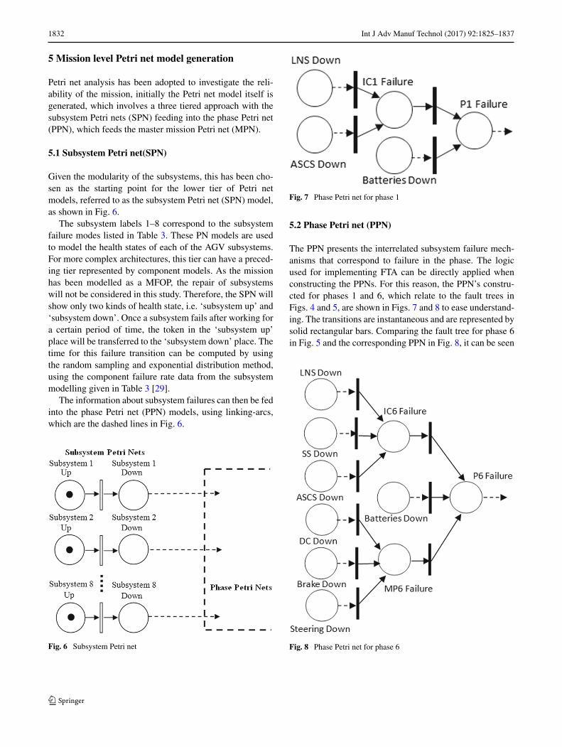
Petri net analysis has been adopted to investigate the reli-ability of the mission, initially the Petri net model itself isgenerated, which involves a three tiered approach with thesubsystem Petri nets (SPN) feeding into the phase Petri net(PPN), which feeds the master mission Petri net (MPN).

5.1 Subsystem Petri net(SPN)

Given the modularity of the subsystems, this has been cho-sen as the starting point for the lower tier of Petri netmodels, referred to as the subsystem Petri net (SPN) model,as shown in Fig. 6.

The subsystem labels 1–8 correspond to the subsystemfailure modes listed in Table 3. These PN models are usedto model the health states of each of the AGV subsystems.For more complex architectures, this tier can have a preced-ing tier represented by component models. As the missionhas been modelled as a MFOP, the repair of subsystemswill not be considered in this study. Therefore, the SPN willshow only two kinds of health state, i.e. ‘subsystem up’ and‘subsystem down’. Once a subsystem fails after working fora certain period of time, the token in the ‘subsystem up’place will be transferred to the ‘subsystem down’ place. Thetime for this failure transition can be computed by usingthe random sampling and exponential distribution method,using the component failure rate data from the subsystemmodelling given in Table 3 [29].

The information about subsystem failures can then be fedinto the phase Petri net (PPN) models, using linking-arcs,which are the dashed lines in Fig. 6.

Fig. 6 Subsystem Petri net

Fig. 7 Phase Petri net for phase 1

5.2 Phase Petri net (PPN)

The PPN presents the interrelated subsystem failure mech-anisms that correspond to failure in the phase. The logicused for implementing FTA can be directly applied whenconstructing the PPNs. For this reason, the PPN’s constru-cted for phases 1 and 6, which relate to the fault trees inFigs. 4 and 5, are shown in Figs. 7 and 8 to ease understand-ing. The transitions are instantaneous and are represented bysolid rectangular bars. Comparing the fault tree for phase 6in Fig. 5 and the corresponding PPN in Fig. 8, it can be seen

Fig. 8 Phase Petri net for phase 6

Int J Adv Manuf Technol (2017) 92:1825–1837 1833

that there is no place in the PN corresponding to the eventsfor functioning through the previous phases in the fault tree.This is dealt with in the master Petri net described in the fol-lowing section. Tokens are absent from all places in Figs. 7and 8, illustrating that the whole AGV system is in a goodhealth condition. In other words, the presence of a token in aplace will mean the failure of either a subsystem or a phase.

5.3 Master Petri net (MPN)

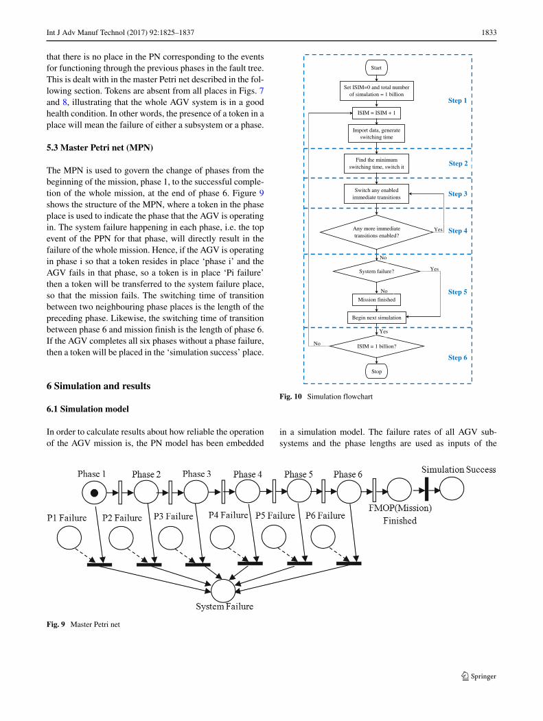
The MPN is used to govern the change of phases from thebeginning of the mission, phase 1, to the successful comple-tion of the whole mission, at the end of phase 6. Figure 9shows the structure of the MPN, where a token in the phaseplace is used to indicate the phase that the AGV is operatingin. The system failure happening in each phase, i.e. the topevent of the PPN for that phase, will directly result in thefailure of the whole mission. Hence, if the AGV is operatingin phase i so that a token resides in place ‘phase i’ and theAGV fails in that phase, so a token is in place ‘Pi failure’then a token will be transferred to the system failure place,so that the mission fails. The switching time of transitionbetween two neighbouring phase places is the length of thepreceding phase. Likewise, the switching time of transitionbetween phase 6 and mission finish is the length of phase 6.If the AGV completes all six phases without a phase failure,then a token will be placed in the ‘simulation success’ place.

6 Simulation and results

6.1 Simulation model

In order to calculate results about how reliable the operationof the AGV mission is, the PN model has been embedded

Start

Set ISIM=0 and total number of simulation = 1 billion

ISIM = ISIM + 1

Import data, generate switching time

Find the minimum switching time, switch it

Switch any enabled immediate transitions

Any more immediate transitions enabled?

System failure?

Mission finished

Begin next simulation

ISIM = 1 billion?

Stop

Yes

Yes

No

No

Yes

No

Step 6

Step 1

Step 2

Step 3

Step 4

Step 5

Fig. 10 Simulation flowchart

in a simulation model. The failure rates of all AGV sub-systems and the phase lengths are used as inputs of the

Fig. 9 Master Petri net

1834 Int J Adv Manuf Technol (2017) 92:1825–1837

PN simulation. Then, the simulation can be programmed byusing the following steps (as illustrated in Fig. 10):

Step 1: Import the phase lengths into the MPN and inparallel, generate the switching time of the transitionsof each subsystem in the SPN’s by using the randomlysampling and exponential distribution method;

Step 2: Find the transition with the minimum switchingtime and then switch it;

Step 3: Search through the immediate transitions that aredirectly connected to the present place. If any are foundenabled, switch them;

Step 4: Repeat Step 3 until no more immediate transitionsare enabled;

Step 5: Test for any of the following conditions and logthem: (a) if system has failed, begin next simulation; (b)if mission has completed, begin next simulation.

Step 6: Iterate the above simulation for n times based onthe assumption that the reliability of the AGV system canbe obtained by repeating the simulation for a sufficientnumber of times.

6.2 Results and validation

Embedding the PN into a simulation, the phase unreliabil-ity and mission reliability have been calculated. The resultsobtained are shown in Table 5 (columns 1–5). In order toensure a good convergence of the computing result, one bil-lion simulations have been performed in the process of thiscalculation. The results have been validated by using theFTA method to calculate the phase and mission reliability(results shown in columns 6 and 7 of Table 5). The com-parison shows that the simulation results obtained from thePN method are very close to the analytical solutions derivedfrom FTA. The simulation errors of both the unreliability

Fig. 11 Convergence of phase 1 unreliability

of each phase and the mission reliability at the end of eachphase are below 1%.

Considering the convergence of the results, Fig. 11 showsthe comparison of the analytical and simulated solution forphase 1 as the number of simulations increases. As can beseen in the figure the value of the unreliability of phase1 obtained from the simulation has converged to the ana-lytical result after performing approximately 100 millionsimulations. Similar results were found for the other phases.Hence, performing 1 billion simulations is sufficient toguarantee the reliability of the calculated result.

From the results presented in Table 5, it is found thatphase 2 ‘dispatch to station’ and phase 4 ‘travelling to stor-age’ show the largest phase unreliability values. This meansthat the AGV is more likely to fail when it is undertaking thetasks of these two phases. Additionally, it is found that themission reliability at the end of the sixth phase is 0.999297,which is based on the success of all six phases. Hence, this

Table 5 PN simulation results

Phase Phase failures Phases started Phaseunreliability

Mission reliabil-ity at phase end

Phase unreliability(FT)

Mission reliabil-ity at phase end(FT)

1 18449 1000000000 0.00001845 0.999982 0.00001855 0.999981

2 244863 999981551 0.00024486 0.999737 0.00024386 0.999738

3 72843 999736688 0.00007286 0.999664 0.00007266 0.999665

4 218911 999663845 0.00021898 0.999445 0.00021915 0.999446

5 22488 999444934 0.00002250 0.999422 0.00002243 0.999423

6 125509 999422446 0.00012558 0.999297 0.00012527 0.999298

Int J Adv Manuf Technol (2017) 92:1825–1837 1835

Table 6 Phase failures during600000 MFOP simulations Phase

Phase started Failures in Total failure Phase unreliability

Mission 1 Mission 2 . . . Mission 500

1 251755556 7 12 . . . 7 4667 0.00001854

2 251750889 162 138 . . . 101 61589 0.00024464

3 251689300 41 54 . . . 47 24193 0.00009612

4 251665107 115 132 . . . 82 55059 0.00021878

5 251610048 11 9 . . . 10 5654 0.00002247

6 251604394 69 75 . . . 66 31552 0.00012540

value also indicates the overall reliability of the AGV inaccomplishing the whole mission. This means that the AGVhas a greater than 99% chance of successfully completingthe mission. For this reason, it can be concluded that theAGV considered here is a very reliable material distributionvehicle in the warehouse. However these are results for onlyone mission and it is expected that the AGV will performnumerous missions and hence its reliability as the number ofmissions increases is of interest. As can be seen from Table5, the mission reliability at the end of each phase decreasesgradually against the number of phases that the AGV hassuccessfully completed. This suggests that without mainte-nance, the more missions are completed, the more unreliablethe AGV system will be.

Hence, the PN model has been run to simulate the AGVsystem performing a number of continuous consecutivemissions without maintenance. The results for 600000 indi-vidual MFOP, each of them containing 500 consecutivemissions, are shown in Table 6, where the unreliability foreach phase is shown. The number of simulations, failuresand reliabilities for each mission and overall MFOP areshown in Table 7. As can be seen, the reliability of the AGVfor completing the MFOP with 500 missions is 0.69547667.Obviously, such a method is very helpful in determining the

Table 7 MFOP and mission failure results

MFOP/mission Starts Failures Reliability

Mission 1 600000 405 0.99932500

Mission 2 599595 420 0.99929953...

.

.

....

.

.

.

Mission 500 417599 313 0.99925048

MFOP 600000 182714 0.69547667

optimal inspection interval for performing the maintenanceof the AGV.

Following this logic, the reliability of the MFOPs withdifferent number of consecutive missions is calculated viasimulation. The simulation results are shown in Fig. 12,from which it is clearly observed that the reliability of theAGV is reduced with the increasing number of missions.Accordingly, through observing such a decreasing tendencyof the reliability of the AGV against the number of missions,the optimal inspection and maintenance time can be readilyestimated to ensure the reliability of the AGV can be abovea desired level.

The research documented in this paper demonstrates thatthe PN method can be used for AGV reliability assessment.It can easily be adapted to cater for varying complexities ofthe subsystems and number of AGVs, where coloured Petrinets can be used. In contrast to the fault tree approach, thePN simulation method does not require finding a complexqualitative solution. Hence, it is a promising time savingand effective approach that can be widely used in the futureto deal with the reliability problems existing in complexsystems.

0

0.2

0.4

0.6

0.8

1

1.2

0 500 1000 1500 2000

Rel

iabi

lity

Number of mission that AGV has completed without maintenance

Fig. 12 Reliability vs. mission number

1836 Int J Adv Manuf Technol (2017) 92:1825–1837

7 Conclusions

In order to develop an efficient and reliable approach toassessing the reliability of AGVs, the PN method is adoptedin this paper to calculate the mission and phase reliabilityof a typical AGV transport system. Due to the size of thesystem considered and the mission profile, FTA was alsoperformed and the results compared with those obtainedusing PN’s. Agreement was seen to be good. FTA is lim-ited in its use for complex systems as dependencies cannotbe accurately modelled. It is also increasingly complexand slow as the number of phases in a mission increases.PNs have none of these limitations and hence can eas-ily be extended to more complex systems and missionswith numerous phases. Through this research, the follow-ing conclusions can be drawn: (1) the PN method has beendemonstrated to be an effective approach for conductingAGV system mission reliability assessment providing thecapability to make informed decisions regarding the accept-ability of AGV mission performance; (2) the results havesuggested that the AGV is more likely to fail when complet-ing the phase ‘dispatch to station’ and the phase ‘travellingto storage’. It is worthy to note that such a judgement ismade only based on the assumptions given in Tables 1and 3. In reality, the judgement result would be different,depending on the environmental, loading and operationalconditions of the AGVs. These are easily adapted withinthe modelling approach thus enabling more complex AGVsystems to be modelled; (3) by using the PN method, theinfluence of maintenance and the optimal time for main-tenance can be evaluated. (4) The PN method is able toaccount for dependencies which may occur within subsys-tem and across mission phases enabling reliable capabilityevaluations for AGV systems of the future with expandingfleets.

It is worth mentioning that if the AGV system is rela-tively simple with no dependencies and the mission does notinvolve multiple tasks then FTA is applicable. However, ifany complexities are involved or maintenance needs to beconsidered then, as shown here, combining the FTA withPN simulation is an efficient approach.

Future work includes expanding the model to includethe routing problem once failure of an AGV occurs in amulti-AGV system. The mission and route will be anal-ysed simultaneously. Also, it is planned that the proposedmethod will be validated in a real AGV system through thecollaboration with relevant industry partners.

Acknowledgements The work reported in this paper aligns to theworking being researched as part of the EPSRC grant EP/K014137/1.The authors would like to extend thanks to Dr Cunjia Liu at Lough-borough University and Mr Dave Berridge at Automated MaterialsHandling SystemsAssociation for their kind help in preparing this paper.

Open Access This article is distributed under the terms of theCreative Commons Attribution 4.0 International License (http://creativecommons.org/licenses/by/4.0/), which permits unrestricteduse, distribution, and reproduction in any medium, provided you giveappropriate credit to the original author(s) and the source, provide alink to the Creative Commons license, and indicate if changes weremade.

References

1. Vis IF (2006) Survey of research in the design and controlof automated guided vehicle. Eur J Oper Res 170(3):677–709

2. Tuan LA, Koster De MMD (2006) A review of design and controlof automated guided vehicle systems. Eur J Oper Res 171(1):1–23

3. Miljkovic Z, Vukovic N, Mitic M, Babic B (2013) New hybridvision-based control approach for automated guided vehicles. IntJ Adv Manuf Technol 66(1):231–249

4. Bhattacharya R, Bandyopadhyay S (2010) An improved strategyto solve shop deadlock problem based on the study on existingbenchmark recovery strategies. Int J Adv Manuf Technol 47:351–364

5. Giuseppe C, Fabiano M, Liotta G (2013) A network flow basedheuristic approach for optimising AGV. J Intell Manuf 24:405–419

6. Salehipour A, Sepehri MM (2014) Optimal location of work-stations in tandem automated-guided vehicle systems. Int J AdvManuf Technol 72(9):1429–1438

7. Mallikarjuna K, Veeranna V, Reddy K (2016) A new meta-heuristics for optimum design of loop layout in flexible man-ufacturing system with integrated scheduling. Int J Adv ManufTechnol 84(9):1841–1860

8. Wu NQ, Zhou MC (2007) Shortest routing of bidirectionalautomated guided vehicles avoiding deadlock and blocking.IEEE/ASME Trans Mechatron 12(1):63–72

9. Nishi T, Tanaka Y (2012) Petri net decomposition approachfor dispatching and conflict-free routing of bidirectional auto-mated guided vehicle systems. IEEE Trans Syst Man, Cybern42(5):1230–1243

10. Rifai AP, Dawal SZMd, Zuhdi A, Aoyama H, Case K. (2016)Re-entrant FMS scheduling in loop layout with consideration ofmulti loading-unloading stations and shortcuts. Int J Adv ManufTechnol 82(9):1527–1545

11. Vivaldini K, Rocha LF., Martarelli NJ, Becker M, Paulo MoreiraA (2016) Integrated tasks assignment and routing for the estima-tion of the optimal number of AGVS. Int J Adv Manuf Technol82(1):719–736

12. Abdelmaguid TF, Nassef AO (2010) A constructive heuristic forthe integrated scheduling of machines and multiple-load mate-rial handling equipment in job shops. Int J Adv Manuf Technol46(9):1239–1251

13. Hamzheei M, Farahani RZ, Rashidi-Bajgan H (2013) An antcolony-based algorithm for finding the shortest bidirectional pathfor automated guided vehicles in a block layout. Int J Adv ManufTechnol 64(1):399–409

14. Trenkle A, Seibold Z, Stoll T (2013) Safety require-ments and safety functions for decentralized controlledautonomous systems. In: XXIV International Conference onInformation, Communication and Automation Technologies(ICAT)

15. Ebben M (2001) Logistic Control In Automated TransportationNetworks. Ph.D. thesis, University of Twente

Int J Adv Manuf Technol (2017) 92:1825–1837 1837

16. Fazlollahtabar H, Saidi-Mehrabad M (2013) Optimising a multi-objective reliability assessment in multiple AGV manufacturingsystem. Int J Serv Oper Manag 3:352–372

17. Tavana M, Fazlollahtabar H, Hassanzadeh R (2014) A bi-objectivestochastic programming model for optimising automated materialhandling systems with reliability considerations. Int J Prod Res52(19):5597–5610

18. Duran DR, Robinson E, Kornecki AJ, Zalewski J (2013) Safetyanalysis of autonomous ground vehicle optical systems: BayesianBelief Networks Approach Computer Science and InformationSystems (FedCSIS), Federated Conference

19. XYang Wu, XYue Wu (2015) Extended object-oriented Petri netmodel for mission reliability simulation of repairable PMS withcommon cause failures. Reliab Eng Syst Saf 130:109–119

20. Le B, Andrews JD (2014) Modelling wind turbine degradation andmaintenance. Wind Energy 19:571–591

21. Luo JL, Ni HJ, Zhou MC (2015) Control program design for auto-mated guided vehicle systems via Petri nets. IEEE Trans Syst Man,Cybern: Syst 45(1):44–55

22. Nishi T, Maeno R (2010) Petri net decomposition approach tooptimization of route planning problems for AGV systems. IEEETrans Autom Sci Eng 7(3):523–537

23. Petri CA (1962) Kommunikation mit automaten, PhD thesis24. Mura I, Bondavalli A (2001) Markov regenerative stochastic petri

nets to model and evaluate phased mission systems dependability.IEEE Trans Comput 50(12):1337–1351

25. Chew SP, Dunnett SJ, Andrews JD (2008) Phased mission mod-elling of systems with maintenance-free operating periods usingsimulated Petri nets. Reliab Eng Syst Saf 93(7):980–994

26. MacLeod EN, Chiarella M (1993) Navigation and control break-through for automated mobility. Proceedings of the SPIE mobilerobotics VIII, Boston MA

27. Division M (1998) Design for success Ultra Reliable Aircraftproject. Design 212:371–378

28. FMD-97 (1997) Failure Mode/Mechanism Distributions, Reliabil-ity Analysis Center

29. Andrews JD, Moss TR (2002) Reliability and risk assessment, 2ndedn. Professional Engineering Publishing