THE WILLIAM DAVIDSON INSTITUTE AT THE UNIVERSITY OF MICHIGAN

Modeling transition in Central Asia: the Case of Kazakhstan

By: Gilles DUFRENOT, Adelya OSPANOVA & Alain SAND-ZANTMAN

William Davidson Institute Working Paper Number 100 1 October 2010

  1

Modeling transition in Central Asia: the Case of Kazakhstan.

Gilles DUFRENOTUniversité of Aix Marseille, DEFI, and CEPII

Adelya OSPANOVA Université Aix Marseille

Alain SAND-ZANTMAN,

OFCE (Centre de Recherche en Economie de Sciences-Po Paris) and GATE Lyon Saint Etienne (CNRS: UMR5824 – Université Lumière Lyon II - Ecole Normale Supérieure de Lyon).

Abstract

This paper presents a small macro-econometric model of Kazakhstan to study the impact

of various economic policies. It uses a new approach to test the existence of a level

relationship between a dependent variable and a set of regressors, when the characteristics of

the regressors’ non-stationarity are not known with certainty. The simulations provide insights

into the role of a tight monetary policy, higher foreign direct investment, and rises in nominal

wages and in crude oil prices. The results obtained are in line with economic observations and

give some support to the policies chosen as priority targets by the Kazakh authorities for the

forthcoming years.

Keywords: Simulation, Forecasting, Transition, Stabilization, Central Asian

JEL Classification: E17, F47, O53, P39

  2

Modeling transition in Central Asia: the Case of Kazakhstan.

Introduction

During the decade of transition, fostering economic growth and curbing inflation have

been among of the main challenges facing the CIS economies1. Using a macro-econometric

model, this paper aims at illustrating the behavior of the Kazakh economy for this period, up

to the recent international financial mayhem. Among the arguments motivating our choice of

Kazakhstan, we can point out its leading position in Central Asia as the second post-soviet

power (after Russia) in terms of development level and growth rate. Ranking as the ninth

largest country in the world, Kazakhstan is one of the better performers in the region in terms

of external trade and foreign exchange policy. Moreover, the economic reforms have been

more comprehensive than in some other countries in the region2.

Until now, few macro-econometric models exist for this country (and more generally

for its neighbors). One explanation is probably the poor quality of data characterized by

various biases (due to measurement errors, the weight of the “shadow” activities, or the short

time span). Consequently, following Dufrenot and Sand-Zantman (2004) we choose to build a

very simple empirical model building-in a system of error-correction equations. This model is

used to study some key features of the Kazakh economy for the previous period, simulating

the impact of the transition period and external opening. We mimic in particular the impact of

a set of policy measures (monetary policy) or international and external shocks (surge of

foreign direct investment, rise in nominal wages and crude oil price hikes). More specifically,

the motivations for this work are deduced from the following arguments:

1. Transition is sometimes viewed as a catching-up phenomenon to the technology level

of developed countries. International technology transfers are usually proportionate to

foreign direct investment. So, allowing a positive shock on FDI is one way to asses the

effect of reducing the technological gap existing between Kazakhstan and its foreign

partners. Moreover, FDI is a prominent driving force behind the country’s economic

growth, mainly in the booming oil and natural gas industries.

                                                            1 For a comparison of economic performance during the first years of transition, see Havrylyshyn and al. (1998), Berg and al. (1999), Falcetti and al. (2000), Fischer and Sahay (2000), Wyplosz (2000) 2 The issue of reforms in Kazakhstan is discussed in several recent papers (see among others Ramaurthy and Tandberg (2002), Bacalu (2003), Medas (2003)) 

  3

2. The brutal changes in income distribution (and generally the decrease of the labor

share of GDP) are considered as a consequence of the transition break, and often a

condition of a future recovery. In particular, a wage freeze is commonly emphasized

as a cornerstone of a stabilization policy aimed at closing the gap between excessive

aggregate demand and insufficient aggregate supply. Moreover, wage pressures

provoke an acceleration of the inflation rate, leading frequently to hyperinflation in

transition stages. But in the Kazakh case, these arguments did not prevent a gradual

wage expansion since 1995. Furthermore, the modernization of the treasury system

and the “rebalancing” of the policy mix in favor of higher exchange rate flexibility,

were decided simultaneously with the relaxation of the fiscal policy, and the increased

spending toward social objectives. And contrary to the orthodox precepts, this package

did not prevent the improvement of the labor market adjustments, with a fall of

unemployment and a steady growth of real wages. Our simulations shed some light on

the rationality of these measures.

3. As in other CIS countries, the reform strategies adopted by Kazakhstan included trade

liberalization and integration into the global economy with tariffs rationalization and

structural reforms to improve the business environment. An important question is

whether such a package is conducive to growth, through the channel of external

demand. In our simulations, we use the US GDP growth rate as a proxy indicator of

world growth to assess the contribution of the external anchor to the current growth of

GDP.

4. Fourth, Kazakh growth depends highly on the oil industry. Capital inflows mainly

concern the oil sector (half of total foreign direct investment). The oil revenues are

determinant for achieving both internal and external balance. Oil accounts for 25-30%

of the budget resources and part of the inflows are saved to smooth the impact of oil

prices’ volatility in international markets. Besides, oil and gas amount to more than

50% of exports and Kazakhstan has a high endowment in other natural resources

(minerals). We can add that the prices of oil and other extractive industries are

significantly correlated and that productivity gains occur through spillover effects

from the oil sectors to non-oil sectors (in particular the sectors of construction and

transportation). Regarding these different aspects, we can assume that oil price

volatility will have strong implications for the economy: this assumption justifies a

specific simulation.

  4

5. Finally, as a consequence of the relative mistrust in fiscal policy, the monetary policy

became the cornerstone of the macroeconomic package. Among the policies required

to bring inflation down and/or stimulate economic activity, two monetary instruments

have been used by the Kazakh monetary authorities over the recent years: i)

expansionary monetary policies based on reduced refinancing rates and lower reserve

requirements for commercial banks; ii) short-term interest rate increases when curbing

inflation became necessary. In Kazakhstan, the efficiency of an interest rate-based

policy was facilitated by the modernization of the banking sector, the independence of

the Central bank and by the fact that budget deficits were kept under control. All these

factors generate an “interest-rate channel” inexistent in many other CIS countries

(Tobin, 1978, Bernanke, Ben S., Gertler; M., 1995,). How much emphasis must be

placed on lowering inflation and on stimulating economic growth is subject to debate.

In our simulation, we examine the impact of an increase in the short-term interest rate.

According to our simulations, the outcomes are in line with the common knowledge of the

“Kazakhstan observers”, giving some support to the policies chosen as priority targets by the

authorities for the forthcoming years.

The rest of the paper is structured as follows. Section 1 presents the main economic

policies adopted since the USSR collapse. Section 2 contains the empirical estimation of the

model. Section 3 presents the policy experiments. Section 4 deals with the analysis of

structural stability. Conclusions are included in Section 5.

1. Economic development since the independence

“… Economic growth based on an open-market economy with high levels of foreign investment and internal savings: to achieve higher and more sustainable economic growth.”

Kazakhstan 2030 – Strategy - one of seven “key goals”

Kazakhstan is the largest of the republics of the former Soviet Union after Russia.

During the Soviet times, Kazakhstan was a raw materials supplier of the USSR. Since the

independence, Kazakhstan has made considerable progresses in implementing economic and

social reforms on the way to a market economy. While the country has not experienced

political disturbances during the transition period, it has faced numerous economic, social and

environmental challenges (see various IMF Staff country reports).

  5

The first few years of Kazakhstan's independence were characterized by an economic

slump (mostly due to the destabilizing force of the disintegration of the Soviet Union): by

1995 real GDP dropped to 61,4% of its 1990 level. This economic deterioration exceeded the

losses observed during the Great Depression of the 1930s. The wide-ranging inflation

observed in the early 1990s peaked at an annual rate of up to 3000% in the mid-nineties.

Since 1992, Kazakhstan has actively pursued a program of economic reform: in particular, it

owns the strongest banking system in Central Asia and CIS. Moreover, the main market-

oriented reforms included the following measures:

• A substantial privatization of the most part of enterprises (as the small or medium

range firms than the big ones, in the “Three-stage privatization program”

frazmework). As a result, 60% of the capital of privatized enterprises has been

transferred to private ownership.

• The adoption of a convertible and fairly stable currency, the Tenge. The Tenge's

stabilization was due in part to the government's determination to control the state

budget, in part to the availability of an IMF stabilization fund, and in part to the

backing of government reserves of US$1.02 billion in hard currency and gold. The

Tenge was allowed to float and underwent depreciation in April 1999, in reaction to

the Russian and Asian financial crises. Introduction of a free-floating exchange rate

regime has stabilized the financial market and improved competitiveness of

Kazakhstan’s producers, easing the monetization (but speeding up slightly inflation).

• An institutional framework to organize trade unions and collective bargain (Law “On

Labor” in 2000; entry in the International Labor Organization in 1993). The minimum wage

has increased every year since 1993, going from 128 Tenge (less than 1$) per month

in 1993 to 14 374 Tenge per month in 2000 and 60 805 Tenge (about 410$) in 2008.

• A price and interest rate liberalization. Prices are almost completely liberalized in

Kazakhstan, with the exception of some basic foodstuffs. Kazakhstan has also made

significant improvements in its banking sector, moving assertively toward market-

based lending and away from government control over the allocation of capital.

Thanks to the improved economic conditions and the authorities’ achievement of

bringing the inflation rate under control, the banks have increased credit to the

economy and reduced interest rates.

• The elimination of trade distortions (including quantitative restrictions) and an

increasing integration into the international trade and capital flows system.

  6

Kazakhstan has no export tariffs; in 1998, the country issued a resolution decreasing its

average import tariff rate to 9%. Furthermore, Kazakhstan has adopted the international tariff

nomenclature as the basis of its tariff schedule, and its customs valuation rules conform to the

WTO Valuation Agreement (Jensen, J., Training, T., and Tarr, D., 2007). As a result,

from 1994 to 2008, the value of its exports rose from US$ 3.23 billion to US$ 71.18

billion. In that same period, the value of its imports grew from US$ 3.56 billion to

US$ 37.88 billion.

• The introduction of a new “pro market” legislation, including a tax code based on

international standards, an effective bankruptcy law, rules about competition and the

securities market, and other components of the essential legal framework for a market

economy.

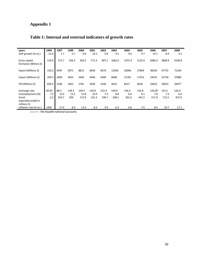
Table 1 (appendix 1) presents some key economic indicators for the Kazakh economy from

1994 to 2008. The main targets of monetary policy were the internal and external stability of

the Tenge and the containment of inflation. During 2000-2001 the authorities have

successfully kept a stable real exchange rate (the credit rating agency Fitch upgraded

Kazakhstan's local currency rating to BBB/Stable) and inflation rates were lower than the

most part of other CIS countries. Since 2002 the guidelines of monetary policy are determined

for a crawling period of three years. It is a kind of transition to the principles of inflation

targeting: the NBK (National Bank of Kazakhstan) now treats price stability as the key

monetary policy target. Its key instruments are open market operations and the official

refinancing rates.

Economic improvement is due to the favorable conditions in the oil sector and its

associated spillover effects. Despite the large efforts of the Kazakh Government to improve

economic diversification, Kazakhstan relies strongly on a petroleum sector linked to all the

other sectors; even for monetary policy, the NBK features scenarios linked to oil prices.

Therefore, Kazakhstan remains highly vulnerable to commodity price fluctuations. When oil

fell to 40 dollars a barrel in early 2009, the economy dived into recession and the currency

depreciated. Thus, diversifying the economy and reducing this resources dependence is a key

issue for the country (the NFRK - National Fund of the Rep. of Kazakhstan - was created in

2001within the National Bank of Kazakhstan to manage the part of national savings coming

from natural resources and to smooth the impact of commodities’ price volatility).

The main driving force behind Kazakhstan's economic growth has been foreign direct

investment. Despite the current international “subprimes” crisis, Kazakhstan continues to

  7

attract a large amount of FDI. Since 1991, Kazakhstan has received more than US$ 30 billion

of foreign direct investment (the highest per capita index in the former Eastern Bloc). If we

analyze transition as a catching-up phenomenon to the technology level of developed

countries, international technology transfers are usually proportionate to foreign investment.

Despite the strong overall economic trends in Kazakhstan, a spiral of unsustainable

growth in commercial credit and foreign borrowing in 2005-2007 set the stage for difficulties

in both the financial and the construction sectors. Since mid-2007, problems in the global

financial markets blocked local banks’ access to cheap external financing. The deepening of

the world economic crisis since September 2008 entailed further negative repercussions on

the country. Kazakhstan faced simultaneously a short but very sharp terms-of-trade shock and

large capital outflows which forced a 20 percent depreciation of the Tenge in February 2009.

GDP growth had decelerated to 3.2 percent in 2008.

Responding to the crisis, the government has enjoined the NFRK to deploy a large

fiscal stimulus program (US$ 8 billion in 2008-2009), focusing on supporting SMEs (small

and medium range enterprises), agriculture, construction, and banks. The latest data suggest

that the stimulus may have met with some success, preventing a more severe recession. Going

forward, the stimulus will need to be reduced, for NFRK cannot be tapped at the same pace as

in 2008, and Kazakhstan intends to contain the buildup of sovereign foreign debt.

 

2. The model: presentation and empirical estimation  

The model is a small, compact, and highly aggregate one. It can be divided into four

blocks - aggregate demand, labor market, prices and monetary policy - with 13 behavioral

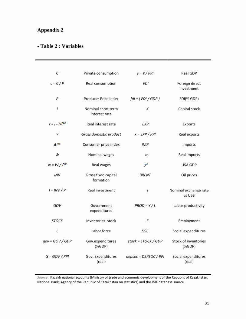
equations and 32 variables. The definitions of the variables are in Table 2 (see Appendix 1).

They are seasonally adjusted and come from the Kazakh national accounts (Ministry of

economy and budget planning of the Republic of Kazakhstan, National Bank, Agency of the

Republic of Kazakhstan on statistics) and the IMF database sources. We use quarterly data

over the period 1994:1 - 2008:4. The model’s ability to reproduce the behavior of the

endogenous variables in an ex post simulation can be regarded as satisfactory. Of course, we

faced the usual problems of empirical time series econometrics (with finite sample, noise,

trends, etc.)

  8

Nonstationarity problems

A first step is to test for the nonstationarity of the variables. The unit root tests, not

reported here, showed mixed results. Some variables were I(0), while others were I(1)4. In

this case, the application of Engle-Granger’s approach would yield misleading conclusions in

terms of cointegration analysis. Given these results, we prefer to use Pesaran, Shin and Smith

(2001)’s methodology (henceforth referred as PSS (2001)). The authors propose a bound

testing approach for the analysis of level relationships which is useful because it can be

applied irrespective of whether the regressors are I(0) or I(1).

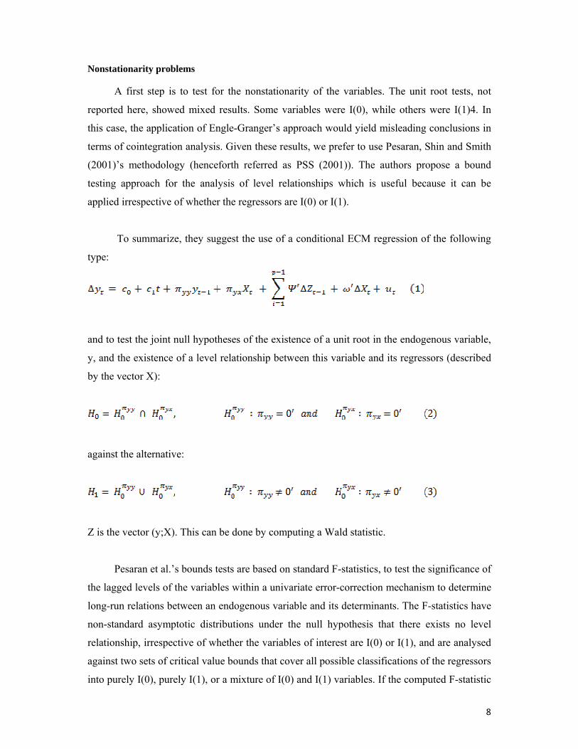
To summarize, they suggest the use of a conditional ECM regression of the following

type:

and to test the joint null hypotheses of the existence of a unit root in the endogenous variable,

y, and the existence of a level relationship between this variable and its regressors (described

by the vector X):

 

against the alternative:

 

Z is the vector (y;X). This can be done by computing a Wald statistic.

Pesaran et al.’s bounds tests are based on standard F-statistics, to test the significance of

the lagged levels of the variables within a univariate error-correction mechanism to determine

long-run relations between an endogenous variable and its determinants. The F-statistics have

non-standard asymptotic distributions under the null hypothesis that there exists no level

relationship, irrespective of whether the variables of interest are I(0) or I(1), and are analysed

against two sets of critical value bounds that cover all possible classifications of the regressors

into purely I(0), purely I(1), or a mixture of I(0) and I(1) variables. If the computed F-statistic

  9

falls outside the critical area, a conclusive decision can be made without needing to know

whether the regressors are I(0) or I(1). That is, if the computed F-statistic falls outside the

lower critical area, we fail to reject the null hypothesis of no level relationship, and if the

computed F-statistic falls outside the upper critical area, then we reject the null hypothesis and

conclude that there exists a level relationship between our variables of interest. On the other

hand, if the computed F-statistic falls within the bounds, then no conclusive inference can be

made without first knowing the order of integration of the variables.

It can be shown that the critical values follow a non standard distribution. These values

are tabulated in PSS (2001). Note that the ways the intercept and the trend are incorporated in

equation (1) refer to a general case. One can envisage different situations (no intercept and no

trend, restricted intercept, restricted trend, etc.). To estimate the PSS ECM equations, we use

a heteroscedastic- and autocorrelation-consistent estimator. We also apply various

misspecification tests to ensure that the residuals of the estimated models are white noise.

       The assumption of a normal distribution of the residuals is tested. The null hypothesis of a

normal distribution is not rejected for any of the equations at the five per cent level (Jarque

Bera test). According to the ARCH test, heteroscedasticity does not appear to pose a problem

in any of the equations. Finally, the Breusch-Godfrey LM test does not reject the null

hypothesis of no serial correlation up to order four for any of the equations at the five per cent

level.

2.1 Aggregate demand

A first set of equations describes the components of aggregate demand: real

consumption, the investment rate, real imports, real exports, changes in stocks, and

Government expenditure.3

 

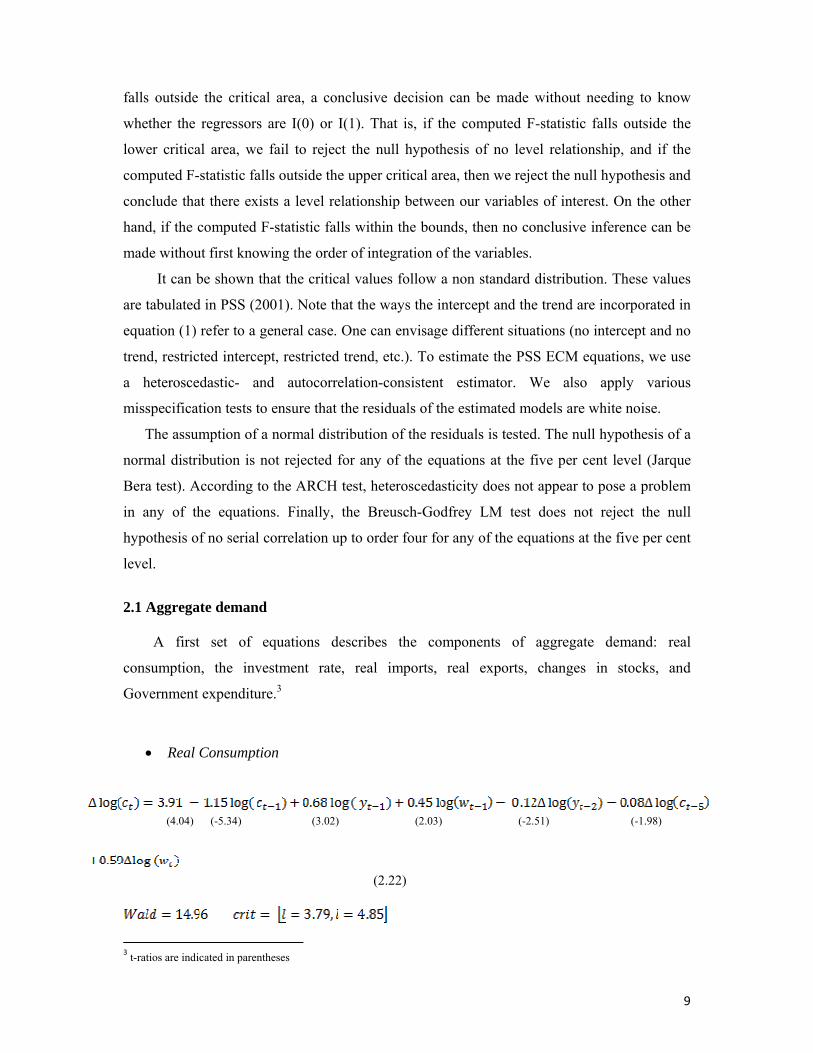
• Real Consumption

(4.04) (-5.34) (3.02) (2.03) (-2.51) (-1.98)

(2.22)

                                                            3 t-ratios are indicated in parentheses 

  10

Where R2 = 0.53; F-statistic = 8.99; Prob(F-Statistic) = 0.0000 and DW = 2.06. The real

private consumption exhibits a significant long-run level relationship with real output. The

result of the PSS test is read as follows. Because this test is based on a bound testing

approach, we have a lower critical value, and an upper critical value . These values depend

upon the number of exogenous variables used in the level (or long-run) relationships.

Here, at the 5% significance level, for k = 2, we have .(see PSS (2001)) The

conclusion is as follows. If the computed Wald statistic lies below then we accept the null

hypothesis, which implies the rejection of a level relationship between the endogenous

variable and its regressors. If instead the computed statistic lies above , we reject the null

hypothesis and conclude in favor of the existence of a level relationship. If we find a

computed statistic in the interval , then it is impossible to conclude. Here, the computed

Wald statistics if higher than the upper critical value, which leads us to conclude in favor of a

level relationship between real consumption and its determinants. We see that the long-run

real output elasticity is less than . The short-run real output coefficient can be

expressed as , so that the coefficient of captures the

influence of real output variability (or volatility) on real consumption. A higher volatility

means more uncertainty about future growth and this encourages saving, thereby implying a

decrease in the propensity to consume. We see that the sensitivity to output uncertainty is

high. As expected, we have a high short-run propensity to consume wages with an elasticity

close to 1.

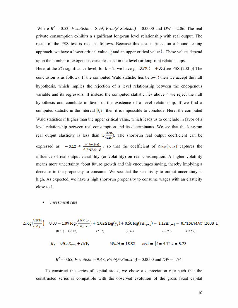
• Investment rate

 

  (0.81) (-6.05) (2.32) (2.32) (-2.90) (-3.57)

                         

R2 = 0.65; F-statistic = 9.48; Prob(F-Statistic) = 0.0000 and DW = 1.74.

To construct the series of capital stock, we chose a depreciation rate such that the

constructed series is compatible with the observed evolution of the gross fixed capital

  11

formation series. We also include a dummy variable in the regression that accounts for the

important fall of real investment during the year 2008. The choice of an appropriate

depreciation rate is subject to debate with regard to the empirical implications. On one hand,

given the important amount of inefficient capital, one could choose a high depreciation rate.

But this choice is not compatible with the statistical properties of the investment series.

Indeed, applying a unit root test, we found that the gross capital formation series was at least

I(1), thereby indicating the presence of an important smooth component in the investment

series. One had to face the question of assuming a depreciation rate compatible with this

statistical property. In this view, one can add the following remarks. Capital stock series are

constructed by accruing investment data. Choosing a high depreciation parameter would

imply that the contribution of investment to capital disappears rapidly (if the assets included

in the capital stock depreciate rapidly, then the contribution of the new flows of capital is

small). The implications are that the capital stock and investment do not evolve in phase.

However, this contradicts several economic observations. In general, investment and capital

stocks share similar downward or upward trends. Further, investment series are more volatile

than capital stock series, thereby implying that the latter have more inertia than the former. As

a consequence, if the investment variable is at least I(1), the capital stock is expected to be at

least I(2). This is the case if one assumes a small depreciation rate in the capital stock

equation, as above.

Foreign direct investment has a positive impact on the investment rate. This estimate

indicates that FDI can help to measure the amount of efficient capital. Each year, the country

receives large inflows of resources, which stimulate development. Finally, we note the

negative and significant impact of the real interest rate and the positive and significant

influence of real output (as expected). The Wald test leads us to conclude that foreign direct

investment is the major determinant of the investment rate in the long-run.

 

• External trade: real exports and real imports

 

  (-4.17) (-4.08) (4.18) (2.55) (-3.65) (3.39)

 

  12

R2 = 0.42; F-statistic = 7.363; Prob(F-Statistic) = 0.00003 and DW = 1.96

  (1.05) (11.9) (-2.36)

 

R2 = 0.75; F-statistic = 52.3; Prob(F-Statistic) = 0.0000 and DW = 1.88 

We choose the American GDP as a proxy for world demand. We do this in regard to the

efforts made by the Kazakh authorities to diversify trade and expand their international links.

Consequently, we find a positive relationship between these variables. It is important to note

that the study of this dependence was not successful during the transition period due to the

previous heavy dependence on Soviet trade routes for input supplies and exports. Since 2000,

when Kazakhstan was recognized as an open market economy, exports began to rise

considerably. Depreciation of the Tenge stimulates the increase of real exports, but foreign

demand and oil prices are the crucial factors that explain real exports, while real imports

heavily depend upon domestic demand. The exogenous variables have long-term effects in the

exports equation, where the assumption of a long-run relationship is accepted. We did not

succeed in finding any role for competitiveness as a determinant of Kazakhstan’s external

balance (this variable was not significant in the regression). The reasons are the following: the

country is a price-taker for a large part of its exports, the price of which is determined by

international markets (gas, oil, grains, cotton, minerals, metals). This is also true for the

imported products (petroleum products, electrical and mechanical equipments, vehicles).

• Changes in inventories

  (6.08) (-3.39) (-6.58)

R2 = 0.65; F-statistic = 32.82; Prob(F-Statistic) = 0.0000 and DW = 1.93

Inventory stocks change in proportion to export growth. So, this equation captures the

fact that inventories serve to meet changes in the demand of Kazakh products by the rest of

the world. Note that, in terms of a stock-adjustment model, the estimation would imply a very

small desired level of stocks (0.000005/0.108). A possible justification of such behavior may

be the structure of the Kazakh external balance. It is known that energy and agricultural

  13

markets are volatile. So, the costs of stocking can become very high, especially during periods

of over-supply and falling prices. Note that this implies a smooth dynamics for stocks (the

previous period level accounts for 68% of the current level).

• Real Government expenditure

  (9.69) (-11.6) (3.37) (-5.24) (-12.08) (-4.4)

 

R2 = 0.86; F-statistic = 43.16; Prob(F-Statistic) = 0.0000 and DW = 1.97

This equation shows that the impact of changes in oil prices has a positive effect on

government expenditure. Higher oil prices imply increased resources in the public finances,

allowing for higher expenditure. The economy depends heavily on the situation in the oil

market. This can have a negative effect related to the variability of the oil price changes. More

volatile prices can increase the uncertainty on future budget resources. This renders future

fiscal balances less likely and exposes the government to capital outflows. To avoid this, the

government may decide to temporarily reduce its expenditure, signaling to the markets its

commitment to meet the budget targets. In Kazakhstan, such behavior has been illustrated by

the creation of a national fund to save part of the inflows to the budget from oil and extractive

industries in order to smooth the impact of price volatility. Moreover, the acceleration of

inflation reduces government consumption and a depreciation of the national currency has a

negative impact through the pressure to the inflation level of the increasing disposable

recourses.

2.2 Labor market

A second set of equations describes the labor market: employment, productivity and

industrial wages.

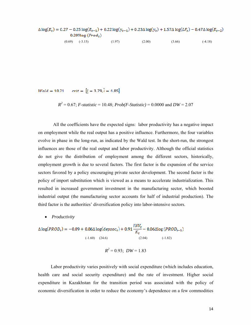
• Employment

  14

  (0.69) (-3.15) (1.97) (2.00) (3.66) (-4.18)

 

 

R2 = 0.67; F-statistic = 10.48; Prob(F-Statistic) = 0.0000 and DW = 2.07

 

All the coefficients have the expected signs: labor productivity has a negative impact

on employment while the real output has a positive influence. Furthermore, the four variables

evolve in phase in the long-run, as indicated by the Wald test. In the short-run, the strongest

influences are those of the real output and labor productivity. Although the official statistics

do not give the distribution of employment among the different sectors, historically,

employment growth is due to several factors. The first factor is the expansion of the service

sectors favored by a policy encouraging private sector development. The second factor is the

policy of import substitution which is viewed as a means to accelerate industrialization. This

resulted in increased government investment in the manufacturing sector, which boosted

industrial output (the manufacturing sector accounts for half of industrial production). The

third factor is the authorities’ diversification policy into labor-intensive sectors.

• Productivity

  (-1.60) (24.6) (2.04) (-1.82)

R2 = 0.93; DW = 1.83

Labor productivity varies positively with social expenditure (which includes education,

health care and social security expenditure) and the rate of investment. Higher social

expenditure in Kazakhstan for the transition period was associated with the policy of

economic diversification in order to reduce the economy’s dependence on a few commodities

  15

(crude oil, natural gas and metals). Such expenditure was viewed as a means to increase labor

productivity through a higher level of human capital, particularly in some sectors such as

petroleum and petrochemical products. The latter are less affected by the world price swings

and have greater value added. The investment rate captures the productivity spillovers and the

foreign direct investment externalities. In Kazakhstan, such spillovers have taken place

through two channels. First, inflows of direct investment financed imports of tradable goods,

such as equipments, that required a high level of human capital. Second, as indicated before,

foreign direct investment induced resource reallocations from the old inefficient activities to

new productive ones.

 

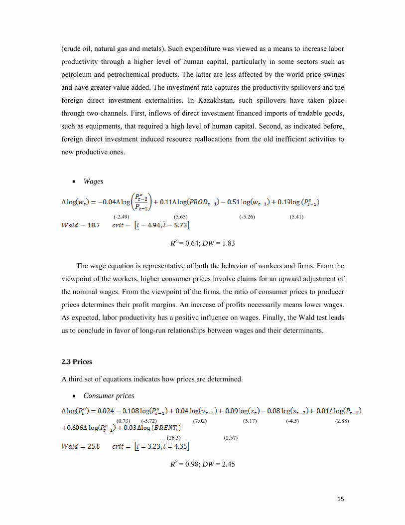
• Wages

  (-2.49) (5.65) (-5.26) (5.41)

 

R2 = 0.64; DW = 1.83 

The wage equation is representative of both the behavior of workers and firms. From the

viewpoint of the workers, higher consumer prices involve claims for an upward adjustment of

the nominal wages. From the viewpoint of the firms, the ratio of consumer prices to producer

prices determines their profit margins. An increase of profits necessarily means lower wages.

As expected, labor productivity has a positive influence on wages. Finally, the Wald test leads

us to conclude in favor of long-run relationships between wages and their determinants.

 

2.3 Prices

A third set of equations indicates how prices are determined.

• Consumer prices

(0.73) (-5.72) (7.02) (5.17) (-4.5) (2.88)

  (26.3) (2.57)

 

R2 = 0.98; DW = 2.45

  16

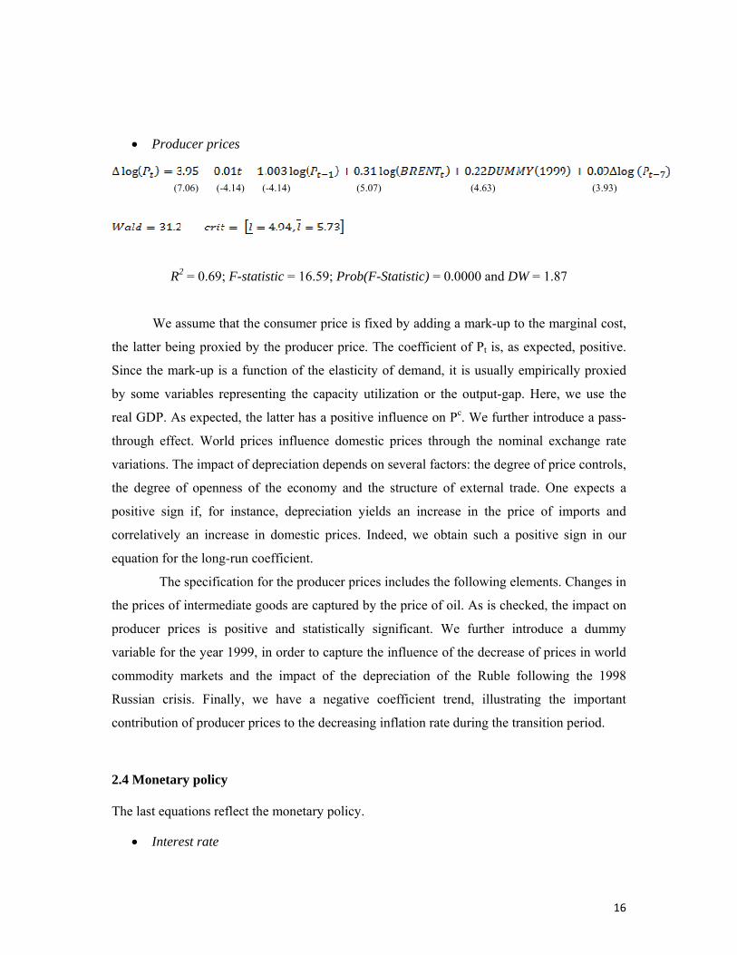
• Producer prices

  (7.06) (-4.14) (-4.14) (5.07) (4.63) (3.93)

 

R2 = 0.69; F-statistic = 16.59; Prob(F-Statistic) = 0.0000 and DW = 1.87 

We assume that the consumer price is fixed by adding a mark-up to the marginal cost,

the latter being proxied by the producer price. The coefficient of Pt is, as expected, positive.

Since the mark-up is a function of the elasticity of demand, it is usually empirically proxied

by some variables representing the capacity utilization or the output-gap. Here, we use the

real GDP. As expected, the latter has a positive influence on Pc. We further introduce a pass-

through effect. World prices influence domestic prices through the nominal exchange rate

variations. The impact of depreciation depends on several factors: the degree of price controls,

the degree of openness of the economy and the structure of external trade. One expects a

positive sign if, for instance, depreciation yields an increase in the price of imports and

correlatively an increase in domestic prices. Indeed, we obtain such a positive sign in our

equation for the long-run coefficient.

The specification for the producer prices includes the following elements. Changes in

the prices of intermediate goods are captured by the price of oil. As is checked, the impact on

producer prices is positive and statistically significant. We further introduce a dummy

variable for the year 1999, in order to capture the influence of the decrease of prices in world

commodity markets and the impact of the depreciation of the Ruble following the 1998

Russian crisis. Finally, we have a negative coefficient trend, illustrating the important

contribution of producer prices to the decreasing inflation rate during the transition period.

 

2.4 Monetary policy

The last equations reflect the monetary policy.

• Interest rate

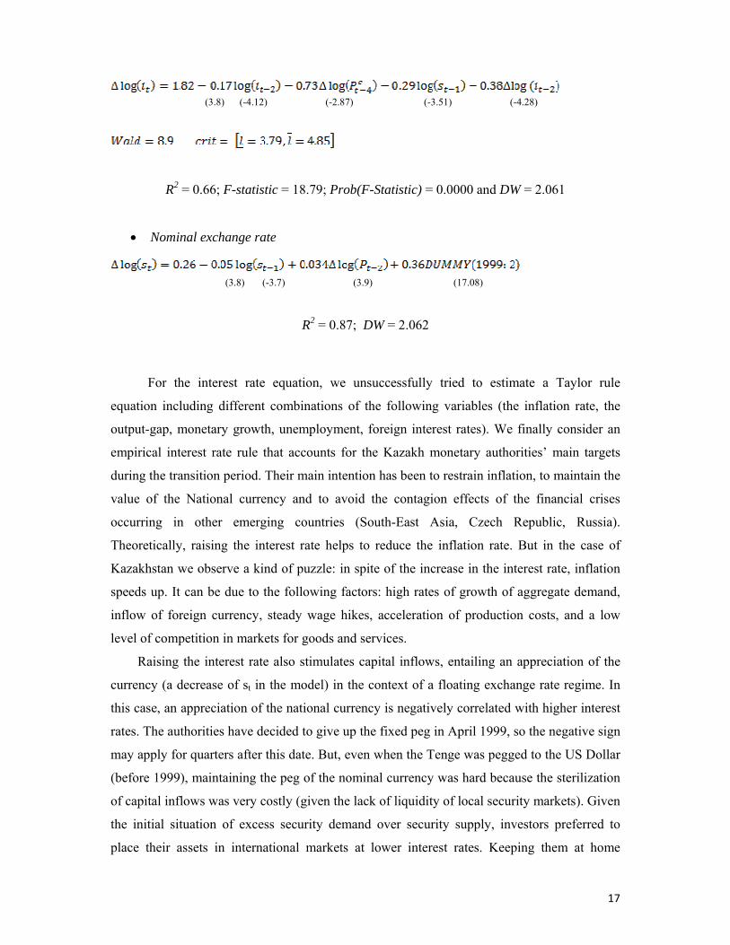
  17

  (3.8) (-4.12) (-2.87) (-3.51) (-4.28)

 

R2 = 0.66; F-statistic = 18.79; Prob(F-Statistic) = 0.0000 and DW = 2.061 

• Nominal exchange rate

  (3.8) (-3.7) (3.9) (17.08)

 

R2 = 0.87; DW = 2.062

 

For the interest rate equation, we unsuccessfully tried to estimate a Taylor rule

equation including different combinations of the following variables (the inflation rate, the

output-gap, monetary growth, unemployment, foreign interest rates). We finally consider an

empirical interest rate rule that accounts for the Kazakh monetary authorities’ main targets

during the transition period. Their main intention has been to restrain inflation, to maintain the

value of the National currency and to avoid the contagion effects of the financial crises

occurring in other emerging countries (South-East Asia, Czech Republic, Russia).

Theoretically, raising the interest rate helps to reduce the inflation rate. But in the case of

Kazakhstan we observe a kind of puzzle: in spite of the increase in the interest rate, inflation

speeds up. It can be due to the following factors: high rates of growth of aggregate demand,

inflow of foreign currency, steady wage hikes, acceleration of production costs, and a low

level of competition in markets for goods and services.

Raising the interest rate also stimulates capital inflows, entailing an appreciation of the

currency (a decrease of st in the model) in the context of a floating exchange rate regime. In

this case, an appreciation of the national currency is negatively correlated with higher interest

rates. The authorities have decided to give up the fixed peg in April 1999, so the negative sign

may apply for quarters after this date. But, even when the Tenge was pegged to the US Dollar

(before 1999), maintaining the peg of the nominal currency was hard because the sterilization

of capital inflows was very costly (given the lack of liquidity of local security markets). Given

the initial situation of excess security demand over security supply, investors preferred to

place their assets in international markets at lower interest rates. Keeping them at home

  18

implied proposing very high interest rates, which would have a depressing effect on real

activity. So, even before 1999, increased interest rates were concomitant with an appreciation

of the Tenge. Note, however, that the appreciation has sometimes implied lowering the

interest rates in order to avoid a Dutch disease.

We finally add a simple formulation of the purchasing power parity condition. The law

of one price implies that any domestic price increase is compensated by a nominal

depreciation. In the above equation, we have an expected positive sign for the coefficient of

the variable ∆log (P). We choose the producer price index because the PPP applies for goods

that are internationally mobile. In the CIS countries, including Kazakhstan, tradable goods

have a stronger influence on producer prices than on consumer prices. We also include a

dummy variable for 1999:2, the date of “de facto floating” of the Tenge (before the official

announcement in April).

3. Policy issues

A wide body of research suggests that growth experience in transition economies,

especially the CIS countries, depends upon the success or failure of the institutional and

structural reforms (see, among many others, Falcetti, Raiser and Sanfey (2000), Havrylyshyn

and Ron van Rooden (2000)). In this work, we omit the institutional aspects of the reforms in

Kazakhstan (due to the non availability of reliable data). More modestly, we study the effects

of different adjustment scenarios, taking the estimations of the previous section as the main

macroeconomic relationships governing Kazakhstan’s economy during the transition period.

Under the assumption that the estimated equations remain valid for the near future, the

simulations used, though they apply to the years 2000:1 -2008:4, can give some flavor of the

macroeconomic adjustment over subsequent years.

 

3.1 The choice of the policy scenarios

We based our simulations on some policy scenarios that the Kazakh authorities found

desirable to reach ten years after the beginning of the transition process and after the opening

to international trade. Further economic development in the Republic of Kazakhstan will also

be ensured by implementing the “Plan of Priority Actions to Ensure Stability of the

Socioeconomic Development of the Republic of Kazakhstan”. According to the authorities’

economic program, as given in different international organizations’ reports (IMF, World

  19

Bank, Asian Development Bank), several macroeconomic policies have been identified as

priority targets (for the years 2010-2011), among which are the following:

1. Taking into account the recent situation on the world markets, three scenarios

for economic development were developed by the monetary authorities

(according to the world oil price levels). The main priority of all scenarios is to

restrain annual inflation within the limits of 6.0-8.0 percent. When inflation will reach

a downward path, there will be scope for some further easing of policy, although it is

important to keep real interest rates at positive levels to support domestic deposits and

help banks to move toward a sustainable funding base. According to the third scenario,

which the NBK considers to be more realistic, the official interest rate will increase to

1%. So, in our simulation, we examine the impact of an increase in the short-term

interest rate of 1 point.

2. Fostering accumulation of new investments in a context of limited domestic

resource mobilization. The accruing of new capital is positively linked to

international technology transfers and acts as a catching-up factor, contributing to

GDP growth. The inflow of foreign direct investment is expected to remain at a high

level in spite of the previsions of a small decrease in 2010 (due to the cuts in funding

for the North-Caspian project, which peaked in 2009). Our purpose is to study the

impact on real activity of a 10% increase in foreign direct investment.

3. Raise the wages of civil servants and employees of public institutions. It was

always one of the priorities of fiscal spending. First, in a context of rapid growth,

increasing wages is a means to ensure that the population reaps the benefits of

growth. This can be viewed as a redistributive policy. In particular, it may help to

flight poverty (the authorities’ goal is to reduce the share of population that has an

income below the poverty line to 20%). A second argument is based on efficiency

wages: increased salaries are an incentive to increase the workers’ labor productivity

and seem essential to attract highly qualified labor. The potential inflationary

pressures of higher wages should be limited by the concomitant increase of labor

productivity. In July 2010 the wage of civil servants will be increased by 30%. We

simulate in our model the impact of a 30% increase in nominal wages.

4. Sustain economic growth, develop the capacity of the deposit market, the

recovery of the credit activity of the banking sector, as well as a public confidence

in the national currency. In Kazakhstan, economic performance is highly influenced

by external factors, in particular changes in the prices of oil, natural gas and metals,

  20

and by the business cycle phases of the trading partner countries. In our simulations,

we envisage two favorable external shocks: an increase of 10$ in the price of crude oil

and an international recovery led by a 10% increase in the US GDP.

3.2 The “structural break” issue:

The specification of the model developed above doesn’t take into account structural

change. Nevertheless, everybody knows that this period has been perturbed by various

mayhems. This might have strong consequences on the stability of the model. The following

steps consist in the detection of eventual structural breaks. We proceed as follows, using the

Kalman filter methodology:

• First, we considered a model with time varying coefficients, and, as usual, we

initialize the vector of parameters by calculating the expected state vector

and the current estimate of state vector .

• Second, we reproduced the path of the parameters of the model to get a value

distribution of each coefficient. This allows us to detect possible changes in the value

of coefficients.

• Finally, we undertake various tests to detect time instability (Appendix 4). In the case

of structural changes, we ran alternative simulations using the models estimated with

the Kalman filter methodology.

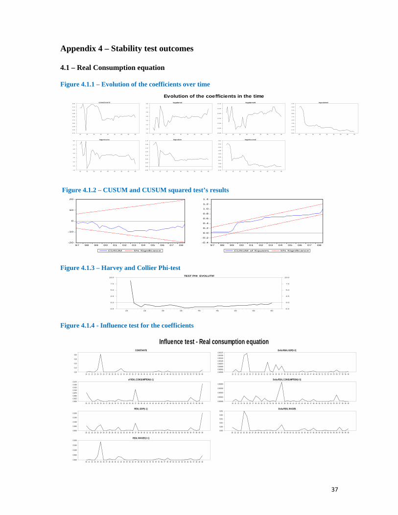
Illustration: the real consumption equation case.

Aiming to initialize the Kalman filter, we use the period 1994:1 - 1998:3. The

calculation of the expected state vector and the current estimate of the state vector start from

the fourth quarter of 1998.

Figure 4.1.1 (in Appendix 4) reproduces the time path of the parameters of the

consumption equation. We note that the filter doesn’t fit quickly, due to the fact that the

greatest fluctuations in the values of the coefficients persist before 2002. The largest part of

fluctuation takes place during the Kazakh transition period. From 2000 onwards, the

parameters became more stable, indicating the beginning of a steady and sustainable growth.

  21

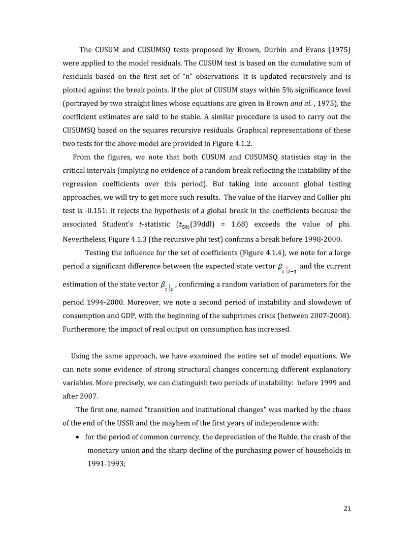
          The  CUSUM  and  CUSUMSQ  tests  proposed  by  Brown,  Durbin  and  Evans  (1975) 

were applied to the model residuals. The CUSUM test is based on the cumulative sum of 

residuals  based  on  the  first  set  of  “n”  observations.  It  is  updated  recursively  and  is 

plotted against the break points. If the plot of CUSUM stays within 5% significance level 

(portrayed by two straight lines whose equations are given in Brown and al. , 1975), the 

coefficient estimates are said to be stable. A similar procedure is used to carry out the 

CUSUMSQ based on the squares recursive residuals. Graphical representations of these 

two tests for the above model are provided in Figure 4.1.2. 

      From  the  figures,  we  note  that  both  CUSUM  and  CUSUMSQ  statistics  stay  in  the 

critical intervals (implying no evidence of a random break reflecting the instability of the 

regression  coefficients  over  this  period).  But  taking  into  account  global  testing 

approaches, we will try to get more such results.  The value of the Harvey and Collier phi 

test  is  ‐0.151:  it rejects the hypothesis of a global break in  the coefficients because the 

associated  Student’s  t‐statistic  ( (39ddl)  =  1.68)  exceeds  the  value  of  phi. 

Nevertheless, Figure 4.1.3 (the recursive phi test) confirms a break before 1998‐2000.  

Testing the influence for the set of coefficients (Figure 4.1.4), we note for a large 

period a significant difference between the expected state vector   and the current 

estimation of the state vector   , confirming a random variation of parameters for the 

period 1994‐2000. Moreover, we note  a  second period of  instability  and  slowdown of 

consumption and GDP, with the beginning of the subprimes crisis (between 2007‐2008). 

Furthermore, the impact of real output on consumption has increased. 

 

     Using  the  same approach, we have examined  the entire  set of model  equations. We 

can note  some evidence of  strong  structural  changes  concerning  different explanatory 

variables. More precisely, we can distinguish two periods of instability:  before 1999 and 

after 2007.   

The first one, named "transition and institutional changes" was marked by the chaos 

of the end of the USSR and the mayhem of the first years of independence with: 

• for the period of common currency, the depreciation of the Ruble, the crash of the 

monetary union and the sharp decline of the purchasing power of households in 

1991‐1993; 

  22

• then the creation of the national currency and the debates about the choice of the 

exchange rate regime during 1993‐1995 (Husain, A.M., 2006). 

• the 1997 Asian crisis, worsening the price competitiveness and export conditions 

of the country; 

• the 1998 Russian crisis (while Russia was the main trade partner of Kazakhstan); 

• the adoption of the freely floating exchange rate in 1999;  

• and  finally,  in  2007,  the  American  crises  of  subprimes  and  the  world  financial 

crisis. 

 

 How can we build‐in the effects of these shocks in new simulations? Because we are in 

non‐linear  cases,  we  cannot  use  the  linear  methods  for  full  period  estimation  and 

simulations. The alternative options to solve this problem are the followings: 

• we  can  use  the  non‐linear  models  (like  Markov‐Switching  VAR  models) 

computing either recursive least squares or rolling regressions (i.e., econometric 

procedures in which the same linear equation is estimated multiple times using 

either a growing sample or partially overlapping subsamples); 

• a more simple solution could be to estimate and run simulations with the model 

using only the period in which we have a full stability of the coefficients (i.e. the 

years 2000 – 2008).  We choose this last solution.        

3.3 Simulation results

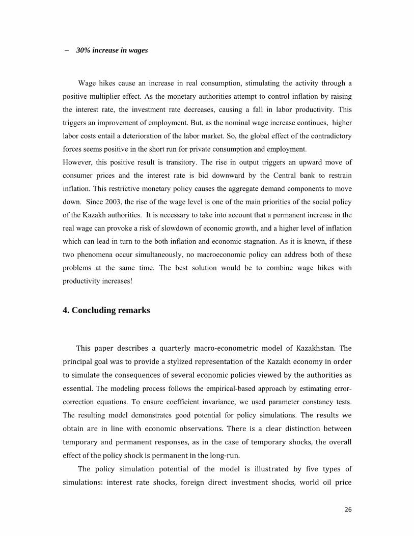
The baseline scenario describes the path of the endogenous variables, solving the

model4. The model aggregates the behavioral equations plus the following national account

identity linking aggregate output and its components (the common deflator is the producer

price index):

 

 

The real output consists in real consumption, real inventory stocks, real investment, real

net exports and real government spending. Appendix 3 reports the difference between the

                                                            4 The model is solved with the nominal variables. Then, the endogenous variables are expressed in real terms. 

  23

simulated trajectories after a given shock and the trajectories corresponding to the baseline

scenario. A positive (resp. negative) value indicates an increase (resp. a decrease) of a

variable in comparison to its baseline value. All the shocks are permanent ones

− 10% permanent increase in foreign direct investment

As shown in Figure 3.1 (Appendix 3 – results of the simulations), a higher amount of

foreign direct investment (FDI) results in a rise in output. FDI yields an increase in real

investment, creating a positive multiplier effect on the components of the GDP: real

consumption, imports. In response to the output boom, government expenditure rises,

allowing wage hikes. The increase of wages and real consumption entail more inflation. More

precisely, the inflows of FDI push interest rates downwards at first. Indeed, FDI concerns

essentially the oil sector while the business climate remains less dynamic in other activities.

On the supply side, FDI affects factor productivity. More generally, in spite of the demand

effects, higher FDI can be viewed as a restructuring factor helping to close the gap between

the excessive aggregate demand and the aggregate supply. The upturn of the output and its

components may thus be interpreted as an adjustment process. Our simulations sum up these

forces, showing the positive impact of increased FDI, both on the demand side (multiplier

effects) and supply side of the economy (productivity effects).  

 

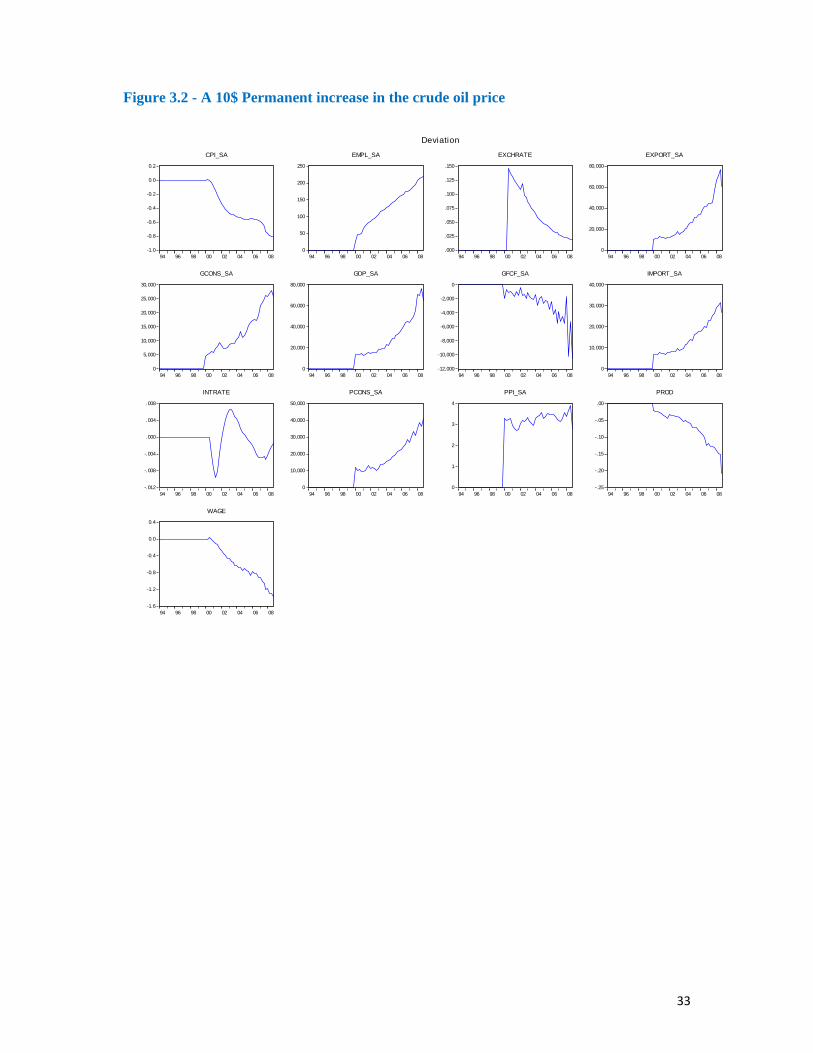
− Permanent increase in the crude oil price of 10$

 

An exogenous shock on the oil price boosts exports (usually rises in energy prices are

correlated with a positive turnaround of world demand) and drives producer prices upward

(because oil products enter as intermediate goods in the domestic products). The favorable

conditions in this case contribute to a rise in GDP. The law of one price in international

markets implies a depreciation of the nominal exchange rate. The impact of the rises in oil

prices on inflation is limited in accordance with the increasing importance given by the

monetary authorities to the control of inflation targets. Probably, measures of the authorities

to diversify the economy and the objectives of the monetary policy were successful.

As shown in Figure 3.2, the nominal wages decrease sharply (in response to the

decrease of consumer prices). The positive multiplier effect explains why employment rises

(the real wages and productivity have decreased). Notice that the multiplier effect is

  24

reinforced by the fact that increased oil prices imply higher resources for the government and

thus higher public spending.

Finally, it can be noted that the monetary authorities modify their behavior over time.

We see that the interest rate is first lowered and then raised. The explanation is that the

nominal interest rate enters as a target in the Central Bank’s reaction function (see the interest

rate equation). The depreciation of the nominal exchange rate improves external

competitiveness, which is favorable for both external and internal balances. This reduces the

inflationary pressures and allows following an accommodative monetary policy.

 

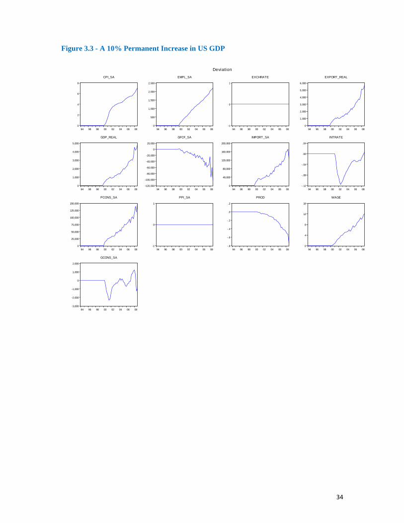
− 10% permanent increase in US GDP

 

The reforms undertaken by Kazakhstan during the transition period implied lower trade

barriers and a higher diversification of external trade. Analyzing the contribution of aggregate

demand to growth, it is important to acknowledge that the country’s growth rate has been

heavily influenced by the world business cycle (this is a major difference with other CIS

countries whose growth has continued to depend upon Russian growth). Here, we study the

impact of a world expansion led by a strong recovery in the USA. The implications are those

expected. As observed in Figure 3, the result is a jump in exports, causing the output

components to adjust upward through a positive multiplier effect. This creates a rise in the

real wage and higher consumer prices as a consequence. If the central Bank reacts by raising

the interest rate later, among the different components of aggregate demand, investment is the

only variable durably negatively affected. Lower investment brings labor productivity down

and this raises employment. As a whole, the simulations show features that are common in

export-oriented growth countries. The positive impact of the foreign growth compensates the

negative effects of a restrictive monetary policy.

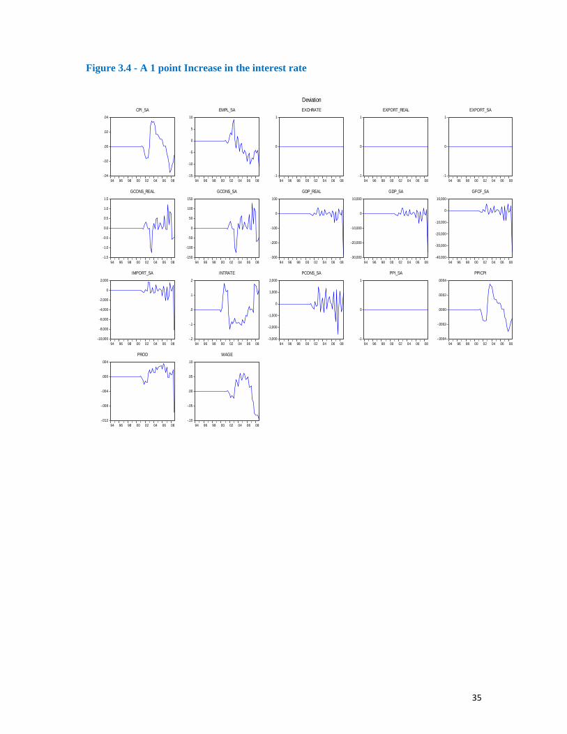
− 1 point permanent increase in the interest rate

The National Bank sets the official refinancing rate according to the situation on the

money market and the inflation rate. So the refinancing rate stays positive in real terms with

increasing inflation, and will be the upper limit of rates at the short-term money currency

market.

  25

An increase in the interest rate tightens monetary policy, making the access to credit

difficult and, consequently, slowing investment. These measures cause a contraction of GDP

components, deteriorating the labor market. The slow increase in the interest rate curbs the

consumer price level. The reaction of wages is not monotonous, because of the increase of

volatility. This fact can be explained by the strong government policy of permanent year-per-

year increase of the wage level in the country. A higher interest rate, by lowering the rate of

investment, also induces a decrease in labor productivity, yielding an upward shift of

employment. The negative response of labor productivity can be interpreted as the result of

the loss of productivity spillovers and positive externalities incorporated in the capital stock.

A lower investment rate in transition economies is synonymous of modernization, which

implies layoffs, in the short-run, as firms reduce their inefficient capital. This has two

implications. The workers can change their skills and move to activities with more value

added. They can choose to work in activities that are more labor intensive, which implies that

they accept lower real wages. Kazakhstan’s situation seems more in line with the second

explanation. The country lacks highly qualified workers and furthermore, the authorities have

been looking for ways to diversify into labor intensive sectors. An exogenous increase in the

interest rate thus generates a positive price-output and price-employment correlation over the

business cycle but a negative price-employment correlation over the long-run (prices diminish

while employment increases). This comes from the fact that, in our model, employment

responds to both aggregate demand (positively) and productivity (negatively).

In brief, the monetary policy impact (in terms of increased interest rates) on the main

macroeconomic variables is not unambiguous. This question causes some debate among

researchers and economists. In certain cases, it helps to restrain inflation and has a detrimental

effect on output. But if we analyze the development trend of the economy since 1995 and look

into the response of the economy to the change in the monetary policy instruments we can

note some facts. In the period 1994 to 2007, the year 1999 is very important due to the

adoption of the full floating regime of the national currency. So we can analyze first the sub-

period before 1999, and then the sub-period since 2000, characterized by macroeconomic

stability. After 1994 - a period of slowdown and high inflation - the main objective was the

reduction of the inflation rate; so the Central Bank sought to quell inflation using monetary

contraction. Later, substantial increases in the money supply in real terms in 2000-2007 were

offset by a strong economic growth rate. For the same period, the refinance rate has not

played a significant role. Its modifications were rare, and expected by the agents.

  26

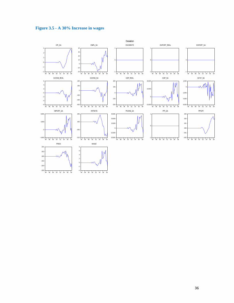
− 30% increase in wages

Wage hikes cause an increase in real consumption, stimulating the activity through a

positive multiplier effect. As the monetary authorities attempt to control inflation by raising

the interest rate, the investment rate decreases, causing a fall in labor productivity. This

triggers an improvement of employment. But, as the nominal wage increase continues, higher

labor costs entail a deterioration of the labor market. So, the global effect of the contradictory

forces seems positive in the short run for private consumption and employment.

However, this positive result is transitory. The rise in output triggers an upward move of

consumer prices and the interest rate is bid downward by the Central bank to restrain

inflation. This restrictive monetary policy causes the aggregate demand components to move

down. Since 2003, the rise of the wage level is one of the main priorities of the social policy

of the Kazakh authorities. It is necessary to take into account that a permanent increase in the

real wage can provoke a risk of slowdown of economic growth, and a higher level of inflation

which can lead in turn to the both inflation and economic stagnation. As it is known, if these

two phenomena occur simultaneously, no macroeconomic policy can address both of these

problems at the same time. The best solution would be to combine wage hikes with

productivity increases!  

4. Concluding remarks  

 

        This  paper  describes  a  quarterly  macro‐econometric  model  of  Kazakhstan.  The 

principal goal was to provide a stylized representation of the Kazakh economy in order 

to simulate the consequences of several economic policies viewed by the authorities as 

essential. The modeling process follows the empirical-based approach by estimating error-

correction equations. To ensure coefficient invariance, we used parameter constancy tests.

The resulting model demonstrates good potential for policy simulations. The  results  we 

obtain  are  in  line  with  economic  observations.  There  is  a  clear  distinction  between 

temporary  and  permanent  responses,  as  in  the  case  of  temporary  shocks,  the  overall 

effect of the policy shock is permanent in the long‐run.  

         The  policy  simulation  potential  of  the  model  is  illustrated  by  five  types  of 

simulations:  interest  rate  shocks,  foreign  direct  investment  shocks,  world  oil  price 

  27

shocks,  foreign  demand  shocks  and  nominal  wage  shocks.  These  sets  of  simulations 

show  the  importance  of  foreign  direct  investments.  These latter can be viewed as a

restructuring factors helping to close the gap between the excessive aggregate demand and the

aggregate supply. Despite  large  efforts  by  the  authorities  to  diversify  the  economy, 

Kazakhstan still  suffers  from a  large dependence on commodity prices. Along with  the 

external  demand  simulations,  they  show  the  vulnerability  of  the  Kazakh  economy  to 

external shocks. We  find that effect of a tight monetary policy  is not unambiguous; we 

argue that in certain cases that is not the most efficient policy instrument. It is possible 

that some combination of measures or short‐run solutions like credit control would be 

the better solution for temporary and exogenously generated disequilibria. It is strongly 

recommended to pay particular attention to the permanent government policy of wage 

expansion due to the possible threat of inflation and economic stagnation, which cannot 

be excluded. 

      However,  the model  suffers  from  some  limitations  that need  to  be mentioned.  The 

specification and estimation of an econometric model for an economy in transition, such 

as Kazakhstan,  are often  complicated by data problems  such  as  short,  inconsistent,  or 

unreliable  time  series.  Nevertheless,  a  simple  model  for  policy  evaluation,  like  that 

which was constructed here, can be developed, fitting empirical data quite well in spite 

of  the  short  time  horizon.  Of  course,  there  are  still  several  specification  issues  and 

statistical  features that may be subject to objections from a theoretical or econometric 

point of view.  

Second,  policy  reforms  are  accompanied  by  institutional  transformations  that 

imply changes of the economic structure. So, we cannot absolutely take for granted that 

the  simulations  done  here  should  characterize  Kazakhstan  for  the  future  years. 

However, this criticism leads us to formulate the following remarks. Until the transition 

is  completed,  structural  changes will  occur. This means  that any model describing  the 

current  situation  of  the  CIS  countries  cannot  be  extrapolated  into  the  future.  A more 

serious  argument  is  the  following.  The main  problem  posed  by  structural  changes  in 

macroeconomic models  refers  to  the  so‐called Lucas‐critique:  the policies may be non 

operating if they induce reactions from the agents. Our model contains no assumptions 

concerning  the  domestic  agents’  expectations.  In  Kazakhstan  and  other  CIS  countries, 

the  agents  that  react  to  policy  decisions  are  international  organizations  (IMF,  World 

Bank, Bank  for Development and Reconstruction  ...). Private  investors, before  taking a 

  28

decision,  refer  to  these organizations’  viewpoint  concerning  the  economic  situation  of 

the  countries.  But  unlike  what  is  observed  in  the  case  of  domestic  agents,  the 

international organizations cannot directly modify  the  impacts  of a  given policy. What 

they do is to provide a general operating framework to implement the policies. 

         This  paper  also  opens  perspectives  for  a  future  research  agenda.  In  particular,  it 

would be interesting to compare the Kazakhstan case with that of other CIS countries to 

see whether  there are  common  factors underlying  their  economic  growth,  just  as was 

the case for Central and Eastern European countries. Such a study could serve as a basis 

for recommendations for coordinated policies in the Region of Central Asia. 

5. References

− Bacalu, V., 2003, “Financial sector development., in Republic of Kazakhstan”

(Selected issues and Statistical appendix), International Monetary Fund Country

Reportn°03-11 ;

− Berg, A., Borensztein, E., Sahay, R. and J. Zettelmyer, 1999, The evolution of output

in transition economies: explaining the differences, International Monetary Fund

Working Paper, n° 9973;

− Bernanke, Ben S., Gertler; M., 1995, “Inside the Black Box: The Credit Channel of

Monetary Policy Transmission “ Journal of Economic Perspectives, Fall, 9, p. 27-48.

− Brown, R.L., Durbin, J. and Evans, J.M., 1975, “ Techniques for Testing the Constancy of Regression Relationships over Time, ” Journal of the Royal Statistical Society, Ser.B, vol.37, pp.149 – 192.

− Dufrenot, G. & Sand-Zantman, A., 2004, “Structural reforms, macroeconomic

policies and the future of Kazakhstan economy”, Document de travail, OFCE, n°

2004-11, Novembre.

− Falcetti, E., Raiser, M., and Sanfey, 2000, “Defying the odds: initial ocnditions,

reforms and growth in the first decade of transition”, L.S.E. Working Paper, May.

− Fischer, S. and R. Sahay, 2000, “The transition economies after ten years”, National

Bureau of Economic Research Working Paper n°7664;

− Havrylyshyn, O., Izvorski, I. and R. van Rooden, 1998, “Recovery and Growth in

transition economies 1990-98: a stylized regression analysis”, IMF Working Papers

n°98-141;

  29

− Husain, A.M., 2006, «To Peg or Not to Peg: A Template for Assessing the Nobler » ;

IMF Working Paper, WP/06/54.

− Jensen, J., Training, T., and Tarr, D., 2007, “The impact of Kazakhstan accession to

the World Trade Organization: a quantitative assessment”, The World Bank Policy

Research Working Paper 4142, March 2007

− Medas, P., 2003, “The non-oil sector in Kazakhstan: links with the oil industry and

contribution to growth, in Republic of Kazakhstan” (Selected issues and Statistical

appendix), International Monetary Fund Country Report n°03-211;

− Pesaran, M.H., Shin, Y. and R.J. Smith, 2001, “Bounds testing approaches to the

analysis of level relationships”, Journal of Applied Econometrics 16, 289-326.

− Ramamurthy, S. and E. Tandberg, 2002, .Treasury reform in Kazakhstan: lessons for

other countries., International Monetary Fund Working Paper n°02-129;

− Tobin J., 1978, “Monetary policies and the economy: the transmission mechanism “

Southern Economic Journal, 44, pp. 421-431.

− Wyplosz, C., 2000, “The ten years of transformation: macroeconomic lessons”, CEPR

discussion Paper,n°2254;

 

 

 

 

 

 

 

 

 

 

 

 

 

 

 

 

  30

Appendix 1

Table 1: Internal and external indicators of growth rates  

years  1994  1997  1999  2000  2001  2002  2003  2004  2005  2006  2007  2008 GDP growth (% an.)  ‐12.6  1.7  2.7  9.8  13.5  9.8  9.3  9.6  9.7  10.7  8.9  3.2 

 Gross capital formation (Billions $) 

110.6  271.7  326.2  450.2  771.3  907.1  1062.6  1472.4  2122.6  3084.3  3868.9  4190.8   

Export (Millions $)  150.2  

6497  5871  8812  8639  9670  12926  20096  27849  38250  47755  71183 

Import (Millions $)  199.5  4300  3655  5040  6446  6584  8408  12781  17352  23676  32756  37889  FDI (Millions $)  

 659.5 

 2106 

 1852 

 2781 

 

 4556 

 4106 

 4624 

 8317 

 6618 

 10623 

 18453 

 20077 

Exchange rate  60.95  88.3  138.3  144.5  150.9  155.9  149.6  136.0  132.8  126.09  122.5  120.3 Unemployment (%)  7.5  13.0  13.5  12.8  10.4  7.3  8.8  8.4  8.1  7.8  7.3  6.6 Social expenditures(bill in millions $) 

2.2  254.7  294  172.9  191.3  196.7  248.1  301.6  441.5  571.9  712.5  875.9 

Inflation rate (% an.)  1402  17.4  8.4  13.3  8.3  5.9  6.3  6.8  7.5  8.5  10.7  17.1 

Source : the Kazakh national accounts  

 

  31

Appendix 2

- Table 2 : Variables  

Variable  Name  Variable  Name        

C  Private consumption  y = Y / PPI  Real GDP  

c = C / P  Real consumption  FDI  Foreign direct investment 

 P  Producer Price index  fdi = ( FDI / GDP )  FDI(% GDP) 

 i  Nominal short term 

interest rate K  Capital stock 

  

r = i ‐    Real interest rate  EXP  Exports  

Y  Gross domestic product  x = EXP / PPI  Real exports  

∆   Consumer price index  IMP  Imports  

W  Nominal wages  m  Real imports  

w = W /    Real wages    USA GDP  

INV  Gross fixed capital formation 

BRENT  Oil prices   

I = INV / P  Real investment  s  Nominal exchange rate vs US$ 

 GOV  Government 

expenditures PROD = Y / L  Labor productivity 

  

STOCK  Inventories  stock  E  Employment  

L  Labor force  SOC  Social expenditures  

gov = GOV / GDP  Gov.expenditures (%GDP) 

stock = STOCK / GDP  Stock of inventories (%GDP) 

 G = GOV / PPI  Gov .Expenditures 

(real) depsoc = DEPSOC / PPI  Social expenditures 

(real)  

       Source : Kazakh national accounts (Ministry of trade and economic development of the Republic of Kazakhstan, National Bank, Agency of the Republic of Kazakhstan on statistics) and the IMF database source. 

  32

Appendix 3 – Simulation Results

Figure 3.1 - A 10% Permanent increase in foreign direct investment

.0

.2

.4

.6

.8

94 96 98 00 02 04 06 08

CPI_SA

-1,000

-800

-600

-400

-200

0

200

94 96 98 00 02 04 06 08

EMPL_SA

-1

0

1

94 96 98 00 02 04 06 08

EXCHRATE

-1

0

1

94 96 98 00 02 04 06 08

EXPORT_SA

-300

-200

-100

0

100

200

300

94 96 98 00 02 04 06 08

GCONS_SA

0

10,000

20,000

30,000

40,000

50,000

60,000

94 96 98 00 02 04 06 08

GDP_SA

0

20,000

40,000

60,000

80,000

94 96 98 00 02 04 06 08

GFCF_SA

0

4,000

8,000

12,000

16,000

20,000

94 96 98 00 02 04 06 08

IMPORT_SA

-.012

-.010

-.008

-.006

-.004

-.002

.000

94 96 98 00 02 04 06 08

INTRATE

0

2,500

5,000

7,500

10,000

12,500

15,000

94 96 98 00 02 04 06 08

PCONS_SA

-1

0

1

94 96 98 00 02 04 06 08

PPI_SA

.0

.2

.4

.6

.8

94 96 98 00 02 04 06 08

PROD

0.0

0.4

0.8

1.2

1.6

94 96 98 00 02 04 06 08

WAGE

Deviation

  33

Figure 3.2 - A 10$ Permanent increase in the crude oil price

-1.0

-0.8

-0.6

-0.4

-0.2

0.0

0.2

94 96 98 00 02 04 06 08

CPI_SA

0

50

100

150

200

250

94 96 98 00 02 04 06 08

EMPL_SA

.000

.025

.050

.075

.100

.125

.150

94 96 98 00 02 04 06 08

EXCHRATE

0

20,000

40,000

60,000

80,000

94 96 98 00 02 04 06 08

EXPORT_SA

0

5,000

10,000

15,000

20,000

25,000

30,000

94 96 98 00 02 04 06 08

GCONS_SA

0

20,000

40,000

60,000

80,000

94 96 98 00 02 04 06 08

GDP_SA

-12,000

-10,000

-8,000

-6,000

-4,000

-2,000

0

94 96 98 00 02 04 06 08

GFCF_SA

0

10,000

20,000

30,000

40,000

94 96 98 00 02 04 06 08

IMPORT_SA

-.012

-.008

-.004

.000

.004

.008

94 96 98 00 02 04 06 08

INTRATE

0

10,000

20,000

30,000

40,000

50,000

94 96 98 00 02 04 06 08

PCONS_SA

0

1

2

3

4

94 96 98 00 02 04 06 08

PPI_SA

-.25

-.20

-.15

-.10

-.05

.00

94 96 98 00 02 04 06 08

PROD

-1.6

-1.2

-0.8

-0.4

0.0

0.4

94 96 98 00 02 04 06 08

WAGE

Deviation

 

 

 

 

 

 

 

 

 

 

 

  34

Figure 3.3 - A 10% Permanent Increase in US GDP

0

2

4

6

8

94 96 98 00 02 04 06 08

CPI_SA

0

500

1,000

1,500

2,000

2,500

94 96 98 00 02 04 06 08

EMPL_SA

-1

0

1

94 96 98 00 02 04 06 08

EXCHRATE

0

1,000

2,000

3,000

4,000

5,000

6,000

94 96 98 00 02 04 06 08

EXPORT_REAL

0

1,000

2,000

3,000

4,000

5,000

94 96 98 00 02 04 06 08

GDP_REAL

-120,000

-100,000

-80,000

-60,000

-40,000

-20,000

0

20,000

94 96 98 00 02 04 06 08

GFCF_SA

0

40,000

80,000

120,000

160,000

200,000

94 96 98 00 02 04 06 08

IMPORT_SA

-.12

-.08

-.04

.00

.04

94 96 98 00 02 04 06 08

INTRATE

0

25,000

50,000

75,000

100,000

125,000

150,000

94 96 98 00 02 04 06 08

PCONS_SA

-1

0

1

94 96 98 00 02 04 06 08

PPI_SA

-.8

-.6

-.4

-.2

.0

.2

94 96 98 00 02 04 06 08

PROD

0

4

8

12

16

94 96 98 00 02 04 06 08

WAGE

-3,000

-2,000

-1,000

0

1,000

2,000

94 96 98 00 02 04 06 08

GCONS_SA

Deviation

 

 

 

 

 

 

 

 

 

 

  35

Figure 3.4 - A 1 point Increase in the interest rate

-.04

-.02

.00

.02

.04

94 96 98 00 02 04 06 08

CPI_SA

-15

-10

-5

0

5

10

94 96 98 00 02 04 06 08

EMPL_SA

-1

0

1

94 96 98 00 02 04 06 08

EXCHRATE

-1

0

1

94 96 98 00 02 04 06 08

EXPORT_REAL

-1

0

1

94 96 98 00 02 04 06 08

EXPORT_SA

-1.5

-1.0

-0.5

0.0

0.5

1.0

1.5

94 96 98 00 02 04 06 08

GCONS_REAL

-150

-100

-50

0

50

100

150

94 96 98 00 02 04 06 08

GCONS_SA

-300

-200

-100

0

100

94 96 98 00 02 04 06 08

GDP_REAL

-30,000

-20,000

-10,000

0

10,000

94 96 98 00 02 04 06 08

GDP_SA

-40,000

-30,000

-20,000

-10,000

0

10,000

94 96 98 00 02 04 06 08

GFCF_SA

-10,000

-8,000

-6,000

-4,000

-2,000

0

2,000

94 96 98 00 02 04 06 08

IMPORT_SA

-.2

-.1

.0

.1

.2

94 96 98 00 02 04 06 08

INTRATE

-3,000

-2,000

-1,000

0

1,000

2,000

94 96 98 00 02 04 06 08

PCONS_SA

-1

0

1

94 96 98 00 02 04 06 08

PPI_SA

-.0004

-.0002

.0000

.0002

.0004

94 96 98 00 02 04 06 08

PPICPI

-.012

-.008

-.004

.000

.004

94 96 98 00 02 04 06 08

PROD

-.10

-.05

.00

.05

.10

94 96 98 00 02 04 06 08

WAGE

Deviation

 

 

 

 

 

 

 

 

 

 

 

  36

Figure 3.5 - A 30% Increase in wages

-.2

-.1

.0

.1

.2

.3

94 96 98 00 02 04 06 08

CPI_SA

-20

-10

0

10

20

30

40

94 96 98 00 02 04 06 08

EMPL_SA

-1

0

1

94 96 98 00 02 04 06 08

EXCHRATE

-1

0

1

94 96 98 00 02 04 06 08

EXPORT_REAL

-1

0

1

94 96 98 00 02 04 06 08

EXPORT_SA

-6

-4

-2

0

2

4

6

94 96 98 00 02 04 06 08

GCONS_REAL

-600

-400

-200

0

200

400

94 96 98 00 02 04 06 08

GCONS_SA

-200

-100

0

100

200

94 96 98 00 02 04 06 08

GDP_REAL

-10,000

0

10,000

20,000

94 96 98 00 02 04 06 08

GDP_SA

-6,000

-4,000

-2,000

0

2,000

94 96 98 00 02 04 06 08

GFCF_SA

-4,000

0

4,000

8,000

94 96 98 00 02 04 06 08

IMPORT_SA

-.010

-.005

.000

.005

94 96 98 00 02 04 06 08

INTRATE

-20,000

-10,000

0

10,000

20,000

30,000

94 96 98 00 02 04 06 08

PCONS_SA

-1

0

1

94 96 98 00 02 04 06 08

PPI_SA

-.002

-.001

.000

.001

.002

.003

94 96 98 00 02 04 06 08

PPICPI

-.006

-.004

-.002

.000

.002

.004

94 96 98 00 02 04 06 08

PROD

-4

-2

0

2

4

6

8

94 96 98 00 02 04 06 08

WAGE

Deviation

 

 

 

 

 

 

 

  37

Appendix 4 – Stability test outcomes

4.1 – Real Consumption equation

Figure 4.1.1 – Evolution of the coefficients over time

Evolution of the coefficients in the timeCONSTANTE

20 25 30 35 40 45 50 55 602.75

3.00

3.25

3.50

3.75

4.00

4.25

4.50

4.75

5.00

logprivcons

20 25 30 35 40 45 50 55 60-1.3

-1.2

-1.1

-1.0

-0.9

-0.8

-0.7

-0.6

loggdpreal

20 25 30 35 40 45 50 55 600.1

0.2

0.3

0.4

0.5

0.6

0.7

0.8

logsalaire

20 25 30 35 40 45 50 55 60-0.25

0.00

0.25

0.50

0.75

1.00

1.25

1.50

1.75

loggdpreald

20 25 30 35 40 45 50 55 60-0.140

-0.135

-0.130

-0.125

-0.120

-0.115

-0.110

logprivconsd

20 25 30 35 40 45 50 55 60-0.10

-0.09

-0.08

-0.07

-0.06

-0.05

-0.04

-0.03

-0.02

-0.01

logsalaired

20 25 30 35 40 45 50 55 600.50

0.75

1.00

1.25

1.50

1.75

2.00

2.25

2.50

2.75

Figure 4.1.2 – CUSUM and CUSUM squared test’s results

-20

-10

0

10

20

97 98 99 00 01 02 03 04 05 06 07 08

CUSUM 5% Significance

-0.4

-0.2

0.0

0.2

0.4

0.6

0.8

1.0

1.2

1.4

97 98 99 00 01 02 03 04 05 06 07 08

CUSUM of Squares 5% Significance

Figure 4.1.3 – Harvey and Collier Phi-test TEST PHI EVOLUTIF

20 25 30 35 40 45 50 55 60-2.5 -2.5

0.0 0.0

2.5 2.5

5.0 5.0

7.5 7.5

10.0 10.0

Figure 4.1.4 - Influence test for the coefficients

Influence test - Real consumption equationCONSTANTE

20 21 22 23 24 25 26 27 28 29 30 31 32 33 34 35 36 37 38 39 40 41 42 43 44 45 46 47 48 49 50 51 52 53 54 55 56 57 58 59 600.00

0.10

0.20

0.30

0.40

of REAL CONSUMPTION(t-1)

20 21 22 23 24 25 26 27 28 29 30 31 32 33 34 35 36 37 38 39 40 41 42 43 44 45 46 47 48 49 50 51 52 53 54 55 56 57 58 59 600.00000.00250.00500.00750.01000.01250.01500.0175

REAL GDP(t-1)

20 21 22 23 24 25 26 27 28 29 30 31 32 33 34 35 36 37 38 39 40 41 42 43 44 45 46 47 48 49 50 51 52 53 54 55 56 57 58 59 600.0000

0.0050

0.0100

0.0150

0.0200

REAL WAGES (t-1)

20 21 22 23 24 25 26 27 28 29 30 31 32 33 34 35 36 37 38 39 40 41 42 43 44 45 46 47 48 49 50 51 52 53 54 55 56 57 58 59 600.0000

0.0050

0.0100

0.0150

0.0200

Delta REAL GDP(t-2)

20 21 22 23 24 25 26 27 28 29 30 31 32 33 34 35 36 37 38 39 40 41 42 43 44 45 46 47 48 49 50 51 52 53 54 55 56 57 58 59 600.0000000.0000250.0000500.0000750.0001000.0001250.0001500.000175

Delta REAL CONSUMPTION(t-5)

20 21 22 23 24 25 26 27 28 29 30 31 32 33 34 35 36 37 38 39 40 41 42 43 44 45 46 47 48 49 50 51 52 53 54 55 56 57 58 59 600.000000

0.000010

0.000020

0.000030

0.000040

Delta REAL WAGES

20 21 22 23 24 25 26 27 28 29 30 31 32 33 34 35 36 37 38 39 40 41 42 43 44 45 46 47 48 49 50 51 52 53 54 55 56 57 58 59 600.000

0.005

0.010

0.015

0.020

0.025

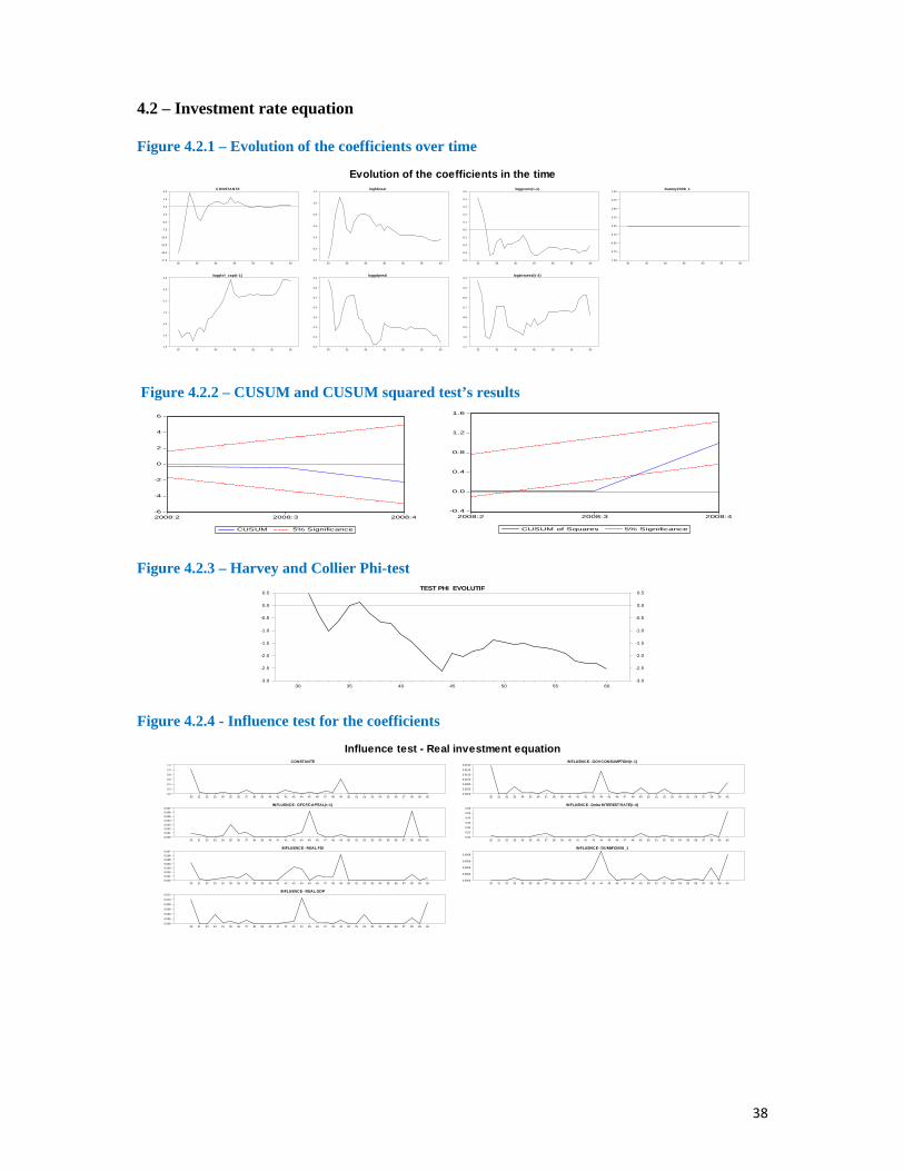
  38

4.2 – Investment rate equation

Figure 4.2.1 – Evolution of the coefficients over time

Evolution of the coefficients in the timeC ON STA NTE

30 35 40 45 50 55 60-17.5

-15.0

-12.5

-10.0

-7.5

-5.0

-2.5

0.0

2.5

5.0

loggfcf_cap(t-1)

30 35 40 45 50 55 60-1.5

-1.4

-1.3

-1.2

-1.1

-1.0

-0.9

logfdireal

30 35 40 45 50 55 600.0

0.2

0.4

0.6

0.8

1.0

1.2

loggdpreal

30 35 40 45 50 55 600.2

0.3

0.4

0.5

0.6

0.7

0.8

0.9

loggcons(t-1)

30 35 40 45 50 55 60-0.4

-0.3

-0.2

-0.1

-0.0

0.1

0.2

0.3

0.4

0.5

logintrated(t-4)

30 35 40 45 50 55 60-1.1

-1.0

-0.9

-0.8

-0.7

-0.6

-0.5

-0.4

dummy2008_1

30 35 40 45 50 55 60-1.00

-0.75

-0.50

-0.25

0.00

0.25

0.50

0.75

1.00

Figure 4.2.2 – CUSUM and CUSUM squared test’s results

-6

-4

-2

0

2

4

6

2008:2 2008:3 2008:4

CUSUM 5% Significance

-0.4

0.0

0.4

0.8

1.2

1.6

2008:2 2008:3 2008:4

CUSUM of Squares 5% Significance

Figure 4.2.3 – Harvey and Collier Phi-test TEST PHI EVOLUTIF

30 35 40 45 50 55 60-3.0 -3.0

-2.5 -2.5

-2.0 -2.0

-1.5 -1.5

-1.0 -1.0

-0.5 -0.5

0.0 0.0

0.5 0.5

Figure 4.2.4 - Influence test for the coefficients

Influence test - Real investment equationCONSTANTE

30 31 32 33 34 35 36 37 38 39 40 41 42 43 44 45 46 47 48 49 50 51 52 53 54 55 56 57 58 59 600.0

0.2

0.4

0.6

0.8

1.0

1.2

INFLUENCE - GFCF/CAPITAL(t-1)

30 31 32 33 34 35 36 37 38 39 40 41 42 43 44 45 46 47 48 49 50 51 52 53 54 55 56 57 58 59 600.0000.0010.0020.0030.0040.0050.0060.007

INFLUENCE - REAL FDI

30 31 32 33 34 35 36 37 38 39 40 41 42 43 44 45 46 47 48 49 50 51 52 53 54 55 56 57 58 59 600.0000.0010.0020.0030.0040.0050.0060.007

INFLUENCE - REAL GDP

30 31 32 33 34 35 36 37 38 39 40 41 42 43 44 45 46 47 48 49 50 51 52 53 54 55 56 57 58 59 600.000

0.002

0.004

0.006

0.008

0.010

0.012

INFLUENCE - GOV CONSUMPTION(t-1)

30 31 32 33 34 35 36 37 38 39 40 41 42 43 44 45 46 47 48 49 50 51 52 53 54 55 56 57 58 59 600.0000

0.0025

0.0050

0.0075

0.0100

0.0125

0.0150

INFLUENCE - Delta INTEREST RATE(t-4)

30 31 32 33 34 35 36 37 38 39 40 41 42 43 44 45 46 47 48 49 50 51 52 53 54 55 56 57 58 59 600.00

0.01

0.02

0.03

0.04

0.05

0.06

INFLUENCE - DUMMY2008_1

30 31 32 33 34 35 36 37 38 39 40 41 42 43 44 45 46 47 48 49 50 51 52 53 54 55 56 57 58 59 600.0000

0.0002

0.0004

0.0006

0.0008

 

 

 

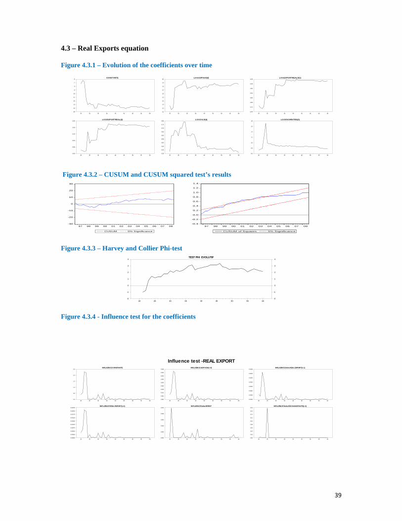
  39

4.3 – Real Exports equation

Figure 4.3.1 – Evolution of the coefficients over time CONSTANTE

20 25 30 35 40 45 50 55 60-15

-14

-13

-12

-11

-10

-9

-8

-7

-6

LOGEXPORTREAL{2}

20 25 30 35 40 45 50 55 60-0.60

-0.55

-0.50

-0.45

-0.40

-0.35

LO GGDPUSA{3}

20 25 30 35 40 45 50 55 601.1

1.2

1.3

1.4

1.5

1.6

1.7

1.8

1.9

2.0

LO GOILD{4}

20 25 30 35 40 45 50 55 600.35

0.40

0.45

0.50

0.55

0.60

0.65

0.70

0.75

0.80

LOGEXPORTREALD{1}

20 25 30 35 40 45 50 55 60-0.75

-0.70

-0.65

-0.60

-0.55

-0.50

-0.45

-0.40

LOGEXCHRATED{3}

20 25 30 35 40 45 50 55 600.6

0.8

1.0

1.2

1.4

1.6

1.8

Figure 4.3.2 – CUSUM and CUSUM squared test’s results

-30

-20

-10

0

10

20

30

97 98 99 00 01 02 03 04 05 06 07 08

CUSUM 5% Significance -0.4

-0.2

0.0

0.2

0.4

0.6

0.8

1.0

1.2

1.4

97 98 99 00 01 02 03 04 05 06 07 08

CUSUM of Squares 5% Significance

Figure 4.3.3 – Harvey and Collier Phi-test TEST PHI EVOLUTIF

20 25 30 35 40 45 50 55 60-2 -2

-1 -1

0 0

1 1

2 2

3 3

4 4

Figure 4.3.4 - Influence test for the coefficients

Influence test -REAL EXPORTINFLUENCE CONSTANTE

20 25 30 35 40 45 50 55 600.0

0.5

1.0

1.5

2.0

2.5

INFLUENCE REAL EXPORT{t-2}

20 25 30 35 40 45 50 55 600.00000

0.00025

0.00050

0.00075

0.00100

0.00125

0.00150

0.00175

0.00200

0.00225

INFLUENCE GDP USA{t-3}

20 25 30 35 40 45 50 55 600.000

0.005

0.010

0.015

0.020

0.025

0.030

0.035

0.040

0.045

INFLUENCE Delta BRENT

20 25 30 35 40 45 50 55 600.000

0.002

0.004

0.006

0.008

0.010

INFLUENCE Delta REAL EXPORT{t-1}

20 25 30 35 40 45 50 55 600.0000

0.0005

0.0010

0.0015

0.0020

0.0025

0.0030

0.0035

INFLUENCE Delta EXCHANGE RATE{t-3}

20 25 30 35 40 45 50 55 600.00

0.02

0.04

0.06

0.08

0.10

0.12

0.14

0.16

0.18

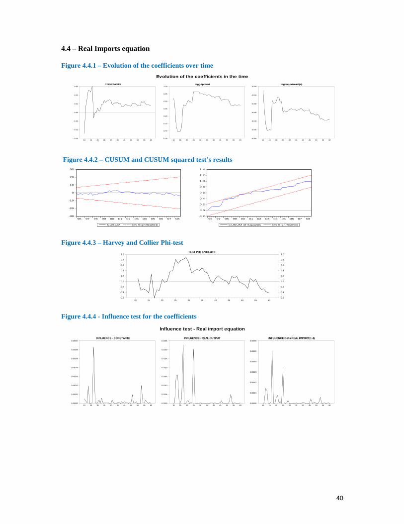
  40

4.4 – Real Imports equation

Figure 4.4.1 – Evolution of the coefficients over time Evolution of the coefficients in the time

CONSTANTE

10 15 20 25 30 35 40 45 50 55 60-0.03

-0.02

-0.01

0.00

0.01

0.02

0.03loggdpreald

10 15 20 25 30 35 40 45 50 55 600.65

0.70

0.75

0.80

0.85

0.90

0.95

1.00logimportreald{4}

10 15 20 25 30 35 40 45 50 55 60-0.050

-0.045

-0.040

-0.035

-0.030

-0.025

-0.020

Figure 4.4.2 – CUSUM and CUSUM squared test’s results

-30

-20

-10

0

10

20

30

96 97 98 99 00 01 02 03 04 05 06 07 08

CUSUM 5% Significance

-0.2

0.0

0.2

0.4

0.6

0.8

1.0

1.2

1.4

96 97 98 99 00 01 02 03 04 05 06 07 08

CUSUM of Squares 5% Significance

Figure 4.4.3 – Harvey and Collier Phi-test TEST PHI EVOLUTIF

10 15 20 25 30 35 40 45 50 55 60-0.6 -0.6

-0.4 -0.4

-0.2 -0.2

0.0 0.0

0.2 0.2

0.4 0.4

0.6 0.6

0.8 0.8

1.0 1.0

Figure 4.4.4 - Influence test for the coefficients

Influence test - Real import equation

INFLUENCE - CONSTANTE

10 15 20 25 30 35 40 45 50 55 600.00000

0.00001

0.00002

0.00003

0.00004

0.00005

0.00006

0.00007INFLUENCE - REAL OUTPUT

10 15 20 25 30 35 40 45 50 55 600.0000

0.0005

0.0010

0.0015

0.0020

0.0025

0.0030

0.0035INFLUENCE Delta REAL IMPORT(t-4)

10 15 20 25 30 35 40 45 50 55 600.00000

0.00001

0.00002

0.00003

0.00004

0.00005

0.00006

  41

4.5 – Changes in inventories equation

Figure 4.5.1 – Evolution of the coefficients in time

Evolution of the coefficients in the time

CONSTANTE

20 25 30 35 40 45 50 55 600.000006

0.000008

0.000010

0.000012

0.000014

0.000016

0.000018

0.000020inventory(t-1)

20 25 30 35 40 45 50 55 60-0.750

-0.725

-0.700

-0.675

-0.650

-0.625

-0.600

-0.575

-0.550logexportreal(t-2)

20 25 30 35 40 45 50 55 60-0.000033

-0.000032

-0.000031

-0.000030

-0.000029

-0.000028

-0.000027

-0.000026

-0.000025

Figure 4.5.2 – CUSUM and CUSUM squared test’s results

-30

-20

-10

0

10

20

30

96 97 98 99 00 01 02 03 04 05 06 07 08

CUSUM 5% Significance

-0.2

0.0

0.2

0.4

0.6

0.8

1.0

1.2

1.4

96 97 98 99 00 01 02 03 04 05 06 07 08

CUSUM of Squares 5% Significance

Figure 4.5.3 – Harvey and Collier Phi-test TEST PHI EVOLUTIF

20 25 30 35 40 45 50 55 60-17.5 -17.5

-15.0 -15.0

-12.5 -12.5

-10.0 -10.0

-7.5 -7.5

-5.0 -5.0

-2.5 -2.5

0.0 0.0

2.5 2.5

Figure 4.5.4 - Influence test for the coefficients

Influence test - Inventory stock equation

CONSTANTE

20 25 30 35 40 45 50 55 600.00000000

0.00000000

0.00000000

0.00000000

0.00000000

0.00000000

0.00000000

0.00000000INVENTORY STOCK(t-1)

20 25 30 35 40 45 50 55 600.0000

0.0005

0.0010

0.0015

0.0020

0.0025

0.0030REAL EXPORT(t-2)

20 25 30 35 40 45 50 55 600.00000000

0.00000000

0.00000000

0.00000000

0.00000000

0.00000000

0.00000000

  42

4.6 – Real Government expenditures equation

Figure 4.6.1 – Evolution of the coefficients over time

Evolution of the coefficients in the timeC ON STA NTE

20 25 30 35 40 45 50 55 604

5

6

7

8

9

10

TR EN D

20 25 30 35 40 45 50 55 60-0.02

-0.01

0.00

0.01

0.02

0.03

0.04

LOGGC ON SR EAL(t-2)

20 25 30 35 40 45 50 55 60-1.6

-1.5

-1.4

-1.3

-1.2

-1.1

-1.0

-0.9

LOGOIL(t-2)

20 25 30 35 40 45 50 55 600.0

0.1

0.2

0.3

0.4

0.5

LOGEXC HR ATED(t-2)

20 25 30 35 40 45 50 55 60-2.00

-1.75

-1.50

-1.25

-1.00

-0.75

-0.50

-0.25

LOGGC ONSR EA LD(t-1)

20 25 30 35 40 45 50 55 60-1.5

-1.4

-1.3

-1.2

-1.1

-1.0

-0.9

-0.8

LOGC PID (t-1)

20 25 30 35 40 45 50 55 60-9

-8

-7

-6

-5

-4

-3

-2

-1

Figure 4.6.2 – CUSUM and CUSUM squared test’s results

-30

-20

-10

0

10

20

30

97 98 99 00 01 02 03 04 05 06 07 08

CUSUM 5% Significance

-0.4

-0.2

0.0

0.2

0.4

0.6

0.8

1.0

1.2

1.4

97 98 99 00 01 02 03 04 05 06 07 08

CUSUM of Squares 5% Significance

Figure 4.6.3 – Harvey and Collier Phi-test TEST PHI EVOLUTIF

20 25 30 35 40 45 50 55 601 1

2 2

3 3

4 4

5 5

6 6

Figure 4.6.4 - Influence test for the coefficients

Influence test - Real government expenditures equationINFLUENCE - CONSTANTE

20 21 22 23 24 25 26 27 28 29 30 31 32 33 34 35 36 37 38 39 40 41 42 43 44 45 46 47 48 49 50 51 52 53 54 55 56 57 58 59 600.000

0.050

0.100

0.150

0.200

INFLUENCE - TREAND

20 21 22 23 24 25 26 27 28 29 30 31 32 33 34 35 36 37 38 39 40 41 42 43 44 45 46 47 48 49 50 51 52 53 54 55 56 57 58 59 600.000000

0.000001

0.000002

0.000003

0.000004

0.000005

0.000006

INFLUENCE - REAL GOV CONSUMPTION(t-2)

20 21 22 23 24 25 26 27 28 29 30 31 32 33 34 35 36 37 38 39 40 41 42 43 44 45 46 47 48 49 50 51 52 53 54 55 56 57 58 59 600.0000

0.0025

0.0050

0.0075

0.0100

INFLUENCE - BRENT(t-2)

20 21 22 23 24 25 26 27 28 29 30 31 32 33 34 35 36 37 38 39 40 41 42 43 44 45 46 47 48 49 50 51 52 53 54 55 56 57 58 59 600.0000

0.0010

0.0020

0.0030

0.0040

INFLUENCE - Delta EXCHANGE RATE(t-2)

20 21 22 23 24 25 26 27 28 29 30 31 32 33 34 35 36 37 38 39 40 41 42 43 44 45 46 47 48 49 50 51 52 53 54 55 56 57 58 59 600.0

0.2

0.4

0.6

0.8

1.0

INFLUENCE - Delta REAL GOV CONSUMPTION(t-1)

20 21 22 23 24 25 26 27 28 29 30 31 32 33 34 35 36 37 38 39 40 41 42 43 44 45 46 47 48 49 50 51 52 53 54 55 56 57 58 59 600.00000

0.00050

0.00100

0.00150

0.00200

INFLUENCE - Delta CPI (t-1)

20 21 22 23 24 25 26 27 28 29 30 31 32 33 34 35 36 37 38 39 40 41 42 43 44 45 46 47 48 49 50 51 52 53 54 55 56 57 58 59 600.0

0.5

1.0

1.5

2.0

2.5

3.0

  43

4.7 – Employment equation

Figure 4.7.1 – Evolution of the coefficients over time CONSTANTE

20 25 30 35 40 45 50 55 60-1.5

-1.0

-0.5

0.0

0.5

1.0

1.5

2.0

2.5

3.0

logempl{1}

20 25 30 35 40 45 50 55 60-0.9

-0.8

-0.7

-0.6

-0.5

-0.4

-0.3

-0.2

loggdpreal{1}

20 25 30 35 40 45 50 55 600.3

0.4

0.5

0.6

0.7

0.8

0.9

1.0

loggdpreald

20 25 30 35 40 45 50 55 600.3

0.4

0.5

0.6

0.7

0.8

0.9

1.0

loglfd

20 25 30 35 40 45 50 55 60-0.5

0.0

0.5

1.0

1.5

2.0

2.5

loglfd{1}

20 25 30 35 40 45 50 55 60-3.0

-2.5

-2.0

-1.5

-1.0

-0.5

0.0

0.5

1.0

1.5

loglfd{2}

20 25 30 35 40 45 50 55 60-0.25

0.00

0.25

0.50

0.75

1.00

1.25

1.50

1.75

2.00

logempld{2}

20 25 30 35 40 45 50 55 60-1.0

-0.8

-0.6

-0.4

-0.2

-0.0

0.2

logprod

20 25 30 35 40 45 50 55 60-1.0

-0.9

-0.8

-0.7

-0.6

-0.5

-0.4

-0.3

Figure 4.7.2 – CUSUM and CUSUM squared test’s results

-30

-20

-10

0

10

20

30

97 98 99 00 01 02 03 04 05 06 07 08

CUSUM 5% Significance

-0.4

-0.2

0.0

0.2

0.4

0.6

0.8

1.0

1.2

1.4

97 98 99 00 01 02 03 04 05 06 07 08

CUSUM of Squares 5% Significance

Figure 4.7.3 – Harvey and Collier Phi-test TEST PHI EVOLUTIF

20 25 30 35 40 45 50 55 60-2 -2

0 0

2 2

4 4

6 6

8 8

10 10

12 12

Figure 4.7.4 - Influence test for the coefficients

Influence test - Employment equationINFLUENCE CONSTANTE

20 25 30 35 40 45 50 55 600.000

0.025

0.050

0.075

0.100

0.125

0.150

0.175

INFLUENCE EMPLOYMENT{t-1}

20 25 30 35 40 45 50 55 600.000

0.001

0.002

0.003

0.004

0.005

0.006

0.007

0.008

INFLUENCE GDP REAL{t-1}

20 25 30 35 40 45 50 55 600.000

0.002

0.004

0.006

0.008

0.010

0.012

0.014

INFLUENCE Delta GDP REAL

20 25 30 35 40 45 50 55 600.000

0.002

0.004

0.006

0.008

0.010

0.012

0.014

INFLUENCE Delta LABOR FORCE

20 25 30 35 40 45 50 55 600.00

0.05

0.10

0.15

0.20

0.25

0.30

0.35

0.40

INFLUENCE Delta LABOR FORCE{t-1}

20 25 30 35 40 45 50 55 600.0

0.2

0.4

0.6

0.8

1.0

1.2

1.4

1.6

INFLUENCE Delta LABOR FORCE{t-2}

20 25 30 35 40 45 50 55 600.0

0.1

0.2

0.3

0.4

0.5

INFLUENCE Delta EMPLOYMENT{t-2}

20 25 30 35 40 45 50 55 600.000

0.002

0.004

0.006

0.008

0.010

0.012

INFLUENCE PRODUCTIVITY

20 25 30 35 40 45 50 55 600.000

0.002

0.004

0.006

0.008

0.010

0.012

0.014

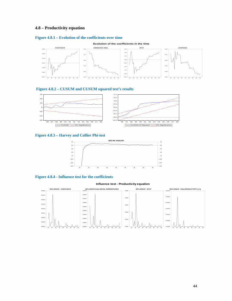
  44

4.8 – Productivity equation

Figure 4.8.1 – Evolution of the coefficients over time Evolution of the coefficients in the time

CONSTANTE

20 25 30 35 40 45 50 55 60-0.075

-0.050

-0.025

0.000

0.025

0.050

0.075EXPENDSOC REAL

20 25 30 35 40 45 50 55 600.83

0.84

0.85

0.86

0.87

0.88GFCF

20 25 30 35 40 45 50 55 60-0.05

-0.04

-0.03

-0.02

-0.01

0.00

0.01

0.02

0.03LOGPRODD

20 25 30 35 40 45 50 55 60-0.035

-0.030

-0.025

-0.020

-0.015

-0.010

Figure 4.8.2 – CUSUM and CUSUM squared test’s results

-30

-20

-10

0

10

20

30

96 97 98 99 00 01 02 03 04 05 06 07 08

CUSUM 5% Significance

-0.2

0.0

0.2

0.4

0.6

0.8

1.0

1.2

1.4

96 97 98 99 00 01 02 03 04 05 06 07 08

CUSUM of Squares 5% Significance

Figure 4.8.3 – Harvey and Collier Phi-test TEST PHI EVOLUTIF

20 25 30 35 40 45 50 55 60-15.0 -15.0

-12.5 -12.5

-10.0 -10.0

-7.5 -7.5

-5.0 -5.0

-2.5 -2.5

0.0 0.0

2.5 2.5

Figure 4.8.4 - Influence test for the coefficients

Influence test - Productivity equation

INFLUENCE - CONSTANTE

20 25 30 35 40 45 50 55 600.00000

0.00025

0.00050

0.00075

0.00100

0.00125

0.00150

0.00175

0.00200INFLUENCE Delta SOCIAL EXPENDITURES

20 25 30 35 40 45 50 55 600.00000

0.00001

0.00002

0.00003

0.00004

0.00005

0.00006

0.00007

0.00008

0.00009INFLUENCE - GFCF

20 25 30 35 40 45 50 55 600.0000

0.0001

0.0002

0.0003

0.0004

0.0005INFLUENCE - Delta PRODUCTIVITY (t-1)

20 25 30 35 40 45 50 55 600.00000

0.00005

0.00010

0.00015

0.00020

0.00025

0.00030

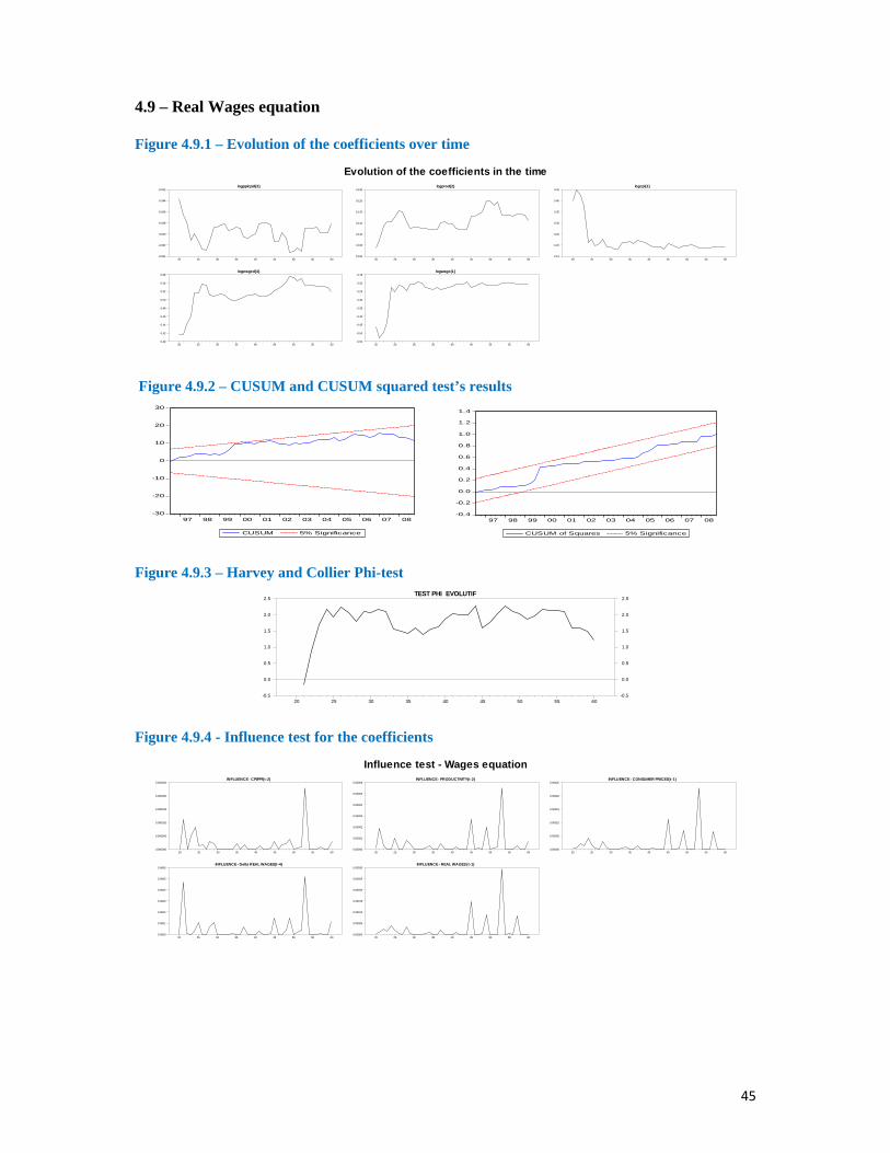
  45

4.9 – Real Wages equation

Figure 4.9.1 – Evolution of the coefficients over time

Evolution of the coefficients in the timelogppicpid{2}

20 25 30 35 40 45 50 55 60-0.054

-0.052

-0.050

-0.048

-0.046

-0.044

-0.042

logwaged{4}

20 25 30 35 40 45 50 55 600.40

0.42

0.44

0.46

0.48

0.50

0.52

0.54

0.56

logprod{2}

20 25 30 35 40 45 50 55 600.100

0.105

0.110

0.115

0.120

0.125

0.130

logwage{1}

20 25 30 35 40 45 50 55 60-0.55

-0.50

-0.45

-0.40

-0.35

-0.30

-0.25

-0.20

-0.15

logcpi{1}

20 25 30 35 40 45 50 55 600.15

0.20

0.25

0.30

0.35

0.40

0.45

Figure 4.9.2 – CUSUM and CUSUM squared test’s results

-30

-20

-10

0

10

20

30

97 98 99 00 01 02 03 04 05 06 07 08

CUSUM 5% Significance

-0.4

-0.2

0.0

0.2

0.4

0.6

0.8

1.0

1.2

1.4

97 98 99 00 01 02 03 04 05 06 07 08

CUSUM of Squares 5% Significance

Figure 4.9.3 – Harvey and Collier Phi-test TEST PHI EVOLUTIF

20 25 30 35 40 45 50 55 60-0.5 -0.5

0.0 0.0

0.5 0.5

1.0 1.0

1.5 1.5

2.0 2.0

2.5 2.5

Figure 4.9.4 - Influence test for the coefficients

Influence test - Wages equationINFLUENCE - CPI/PPI(t-2)

20 25 30 35 40 45 50 55 600.000000

0.000005

0.000010

0.000015

0.000020

0.000025

INFLUENCE - Delta REAL WAGES(t-4)

20 25 30 35 40 45 50 55 600.0000

0.0001

0.0002

0.0003

0.0004

0.0005

0.0006

INFLUENCE - PRODUCTIVITY(t-2)

20 25 30 35 40 45 50 55 600.00000

0.00001

0.00002

0.00003

0.00004

0.00005

0.00006

INFLUENCE - REAL WAGES (t-1)

20 25 30 35 40 45 50 55 600.00000

0.00005

0.00010

0.00015

0.00020

0.00025

0.00030

INFLUENCE - CONSUMER PRICES(t-1)

20 25 30 35 40 45 50 55 600.00000

0.00005

0.00010

0.00015

0.00020

0.00025

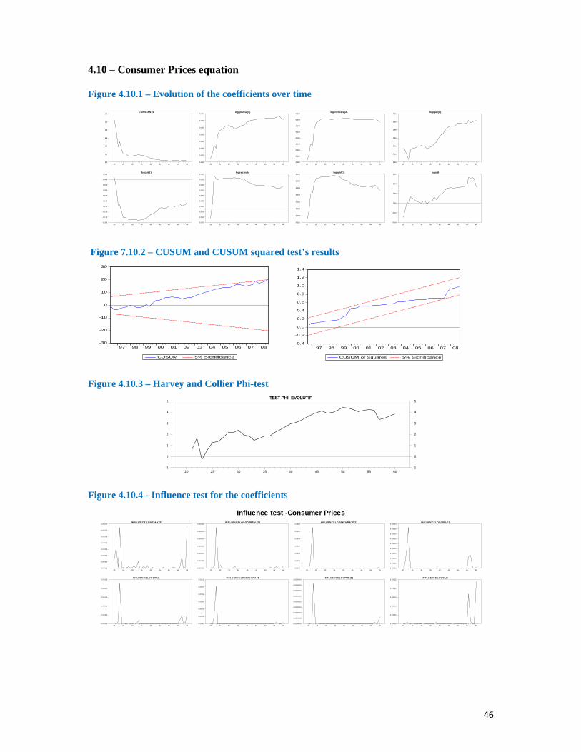
  46

4.10 – Consumer Prices equation

Figure 4.10.1 – Evolution of the coefficients over time CONSTANTE

20 25 30 35 40 45 50 55 600.0

0.2

0.4

0.6

0.8

1.0

1.2

logcpi{1}

20 25 30 35 40 45 50 55 60-0.200

-0.175

-0.150

-0.125

-0.100

-0.075

-0.050

-0.025

-0.000

0.025

loggdpreal{1}

20 25 30 35 40 45 50 55 600.015

0.020

0.025

0.030

0.035

0.040

0.045

0.050

logexchrate

20 25 30 35 40 45 50 55 60-0.075

-0.050

-0.025

0.000

0.025

0.050

0.075

0.100

0.125

0.150

logexchrate{2}

20 25 30 35 40 45 50 55 60-0.250

-0.225

-0.200

-0.175

-0.150

-0.125

-0.100

-0.075

-0.050

logppid{1}

20 25 30 35 40 45 50 55 600.006

0.008

0.010

0.012

0.014

0.016

0.018

0.020

logcpid{1}

20 25 30 35 40 45 50 55 600.35

0.40

0.45

0.50

0.55

0.60

0.65

logoild

20 25 30 35 40 45 50 55 60-0.04

-0.02

0.00

0.02

0.04

0.06

Figure 7.10.2 – CUSUM and CUSUM squared test’s results

-30

-20

-10

0

10

20

30

97 98 99 00 01 02 03 04 05 06 07 08

CUSUM 5% Significance

-0.4

-0.2

0.0

0.2

0.4

0.6

0.8

1.0

1.2

1.4

97 98 99 00 01 02 03 04 05 06 07 08

CUSUM of Squares 5% Significance

Figure 4.10.3 – Harvey and Collier Phi-test TEST PHI EVOLUTIF

20 25 30 35 40 45 50 55 60-1 -1

0 0

1 1

2 2

3 3

4 4

5 5

Figure 4.10.4 - Influence test for the coefficients

Influence test -Consumer PricesIN FLU EN CE CON STAN TE

20 25 30 35 40 45 50 55 600.00000

0.00002

0.00004

0.00006

0.00008

0.00010

0.00012

0.00014

IN FLU EN CE LOGC PI{1}

20 25 30 35 40 45 50 55 600.00000

0.00005

0.00010

0.00015

0.00020

0.00025

INFLUEN CE LOGGDPREA L{1}

20 25 30 35 40 45 50 55 600.000000

0.000005

0.000010

0.000015

0.000020

0.000025

0.000030

INFLUEN CE LOGEXCH RA TE

20 25 30 35 40 45 50 55 600.0000

0.0002

0.0004

0.0006

0.0008

0.0010

0.0012

INFLUENC E LOGEXC HR ATE{2}

20 25 30 35 40 45 50 55 600.0000

0.0002

0.0004

0.0006

0.0008

0.0010

0.0012

INFLUENC E LOGPPID {1}

20 25 30 35 40 45 50 55 600.0000000

0.0000005

0.0000010

0.0000015

0.0000020

0.0000025

0.0000030

0.0000035

0.0000040

IN FLU ENC E LOGCPID{1}

20 25 30 35 40 45 50 55 600.00000

0.00005

0.00010

0.00015

0.00020

0.00025

0.00030

0.00035

0.00040

0.00045

IN FLU ENC E LOGOILD

20 25 30 35 40 45 50 55 600.00000

0.00005

0.00010

0.00015

0.00020

0.00025

  47

4.11 – Producer prices equation

Figure 4.11.1 – Evolution of the coefficients over time

Evolution of the coefficients in the timeCONSTANTE

20 25 30 35 40 45 50 55 602.5

3.0

3.5

4.0

4.5

5.0

5.5

TREND

20 25 30 35 40 45 50 55 60-0.020

-0.015

-0.010

-0.005

0.000

0.005

0.010

LOGPPI(t-1)

20 25 30 35 40 45 50 55 60-1.2

-1.1

-1.0

-0.9

-0.8

-0.7

-0.6

LOGOIL

20 25 30 35 40 45 50 55 600.05

0.10

0.15

0.20

0.25

0.30

0.35

0.40

0.45

0.50

LOGPPID(t-7)

20 25 30 35 40 45 50 55 600.070

0.075

0.080

0.085

0.090

0.095

0.100

0.105

0.110

0.115

DUMMY99

20 25 30 35 40 45 50 55 60-1.00

-0.75

-0.50

-0.25

0.00

0.25

0.50

0.75

1.00

Figure 4.11.2 – CUSUM and CUSUM squared test’s results

-20

-15

-10

-5

0

5

10

15

20

99 00 01 02 03 04 05 06 07 08

CUSUM 5% Significance

-0.4

-0.2

0.0

0.2

0.4

0.6

0.8

1.0

1.2

1.4

99 00 01 02 03 04 05 06 07 08

CUSUM of Squares 5% Significance

Figure 4.11.3 – Harvey and Collier Phi-test TEST PHI EVOLUTIF

20 25 30 35 40 45 50 55 60-3.5 -3.5

-3.0 -3.0

-2.5 -2.5

-2.0 -2.0

-1.5 -1.5

-1.0 -1.0

-0.5 -0.5

0.0 0.0

0.5 0.5

Figure 4.11.4 - Influence test for the coefficients

Influence test - Producer prox equationINFLUENCE - CONSTANTE

20 21 22 23 24 25 26 27 28 29 30 31 32 33 34 35 36 37 38 39 40 41 42 43 44 45 46 47 48 49 50 51 52 53 54 55 56 57 58 59 600.00

0.02

0.04

0.06

0.08

0.10

0.12

INFLUENCE - TREND

20 21 22 23 24 25 26 27 28 29 30 31 32 33 34 35 36 37 38 39 40 41 42 43 44 45 46 47 48 49 50 51 52 53 54 55 56 57 58 59 600.00000000

0.00000050

0.00000100

0.00000150

0.00000200

INFLUENCE - PPI (t-1)

20 21 22 23 24 25 26 27 28 29 30 31 32 33 34 35 36 37 38 39 40 41 42 43 44 45 46 47 48 49 50 51 52 53 54 55 56 57 58 59 600.000

0.002

0.004

0.006

0.008

INFLUENCE - BRENT

20 21 22 23 24 25 26 27 28 29 30 31 32 33 34 35 36 37 38 39 40 41 42 43 44 45 46 47 48 49 50 51 52 53 54 55 56 57 58 59 600.0000

0.0002

0.0004

0.0006

0.0008

0.0010

0.0012

INFLUENCE - Delta PPI (t-7)

20 21 22 23 24 25 26 27 28 29 30 31 32 33 34 35 36 37 38 39 40 41 42 43 44 45 46 47 48 49 50 51 52 53 54 55 56 57 58 59 600.000000

0.000005

0.000010

0.000015

0.000020

0.000025

INFLUENCE - DUMMY99

20 21 22 23 24 25 26 27 28 29 30 31 32 33 34 35 36 37 38 39 40 41 42 43 44 45 46 47 48 49 50 51 52 53 54 55 56 57 58 59 600.00000

0.00005

0.00010

0.00015

0.00020

0.00025

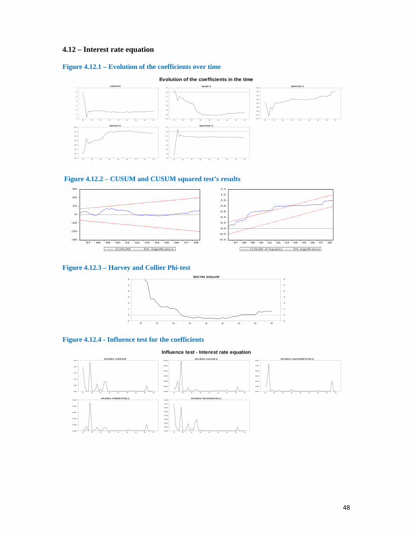
  48

4.12 – Interest rate equation

Figure 4.12.1 – Evolution of the coefficients over time

Evolution of the coefficients in the timeCONSTANTE

20 25 30 35 40 45 50 55 600

1

2

3

4

5

6

7

logintrate(t-2)

20 25 30 35 40 45 50 55 60-0.45

-0.40

-0.35

-0.30

-0.25

-0.20

-0.15

-0.10

logcpid(t-4)

20 25 30 35 40 45 50 55 60-0.6

-0.5

-0.4

-0.3

-0.2

-0.1

-0.0

0.1

logexchrate(t-1)

20 25 30 35 40 45 50 55 60-1.2

-1.0

-0.8

-0.6

-0.4

-0.2

-0.0

0.2

logintrated(t-2)

20 25 30 35 40 45 50 55 60-0.44

-0.42

-0.40

-0.38

-0.36

-0.34

-0.32

-0.30

-0.28

Figure 4.12.2 – CUSUM and CUSUM squared test’s results

-30

-20

-10

0

10

20

30

97 98 99 00 01 02 03 04 05 06 07 08

CUSUM 5% Significance

-0.4

-0.2

0.0

0.2

0.4

0.6

0.8

1.0

1.2

1.4

97 98 99 00 01 02 03 04 05 06 07 08

CUSUM of Squares 5% Significance

Figure 4.12.3 – Harvey and Collier Phi-test TEST PHI EVOLUTIF

20 25 30 35 40 45 50 55 60-1 -1

0 0

1 1

2 2

3 3

4 4

5 5

6 6

Figure 4.12.4 - Influence test for the coefficients

Influence test - Interest rate equationINFLUENCE - CONSTANTE

20 25 30 35 40 45 50 55 600.000

0.005

0.010

0.015

0.020

0.025

INFLUENCE - INTEREST RATE(t-2)

20 25 30 35 40 45 50 55 600.00000

0.00005

0.00010

0.00015

0.00020

0.00025

INFLUENCE - Delta CPI(t-4)

20 25 30 35 40 45 50 55 600.00000

0.00025

0.00050

0.00075

0.00100

0.00125

0.00150

INFLUENCE - EXCHANGE RATE (t-1)

20 25 30 35 40 45 50 55 600.0000

0.0001

0.0002

0.0003

0.0004

0.0005

0.0006

0.0007

0.0008

INFLUENCE - Delta INTEREST RATE(t-2)

20 25 30 35 40 45 50 55 600.0000

0.0002

0.0004

0.0006

0.0008

0.0010

0.0012

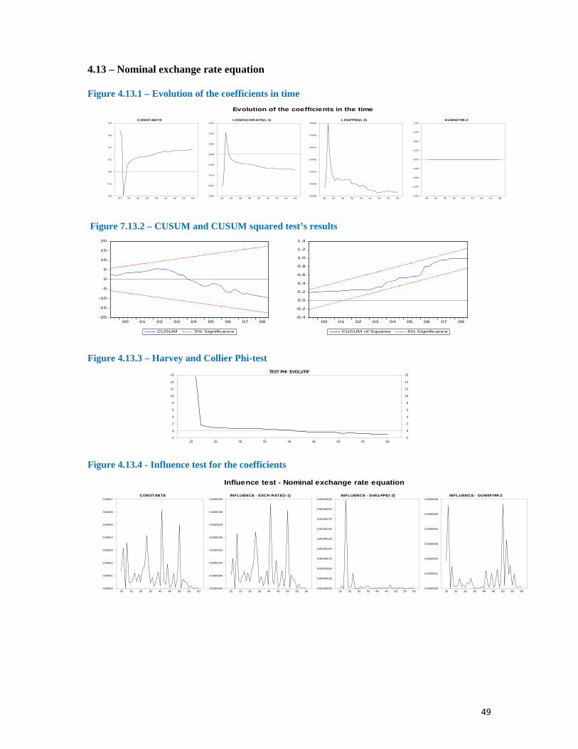
  49

4.13 – Nominal exchange rate equation

Figure 4.13.1 – Evolution of the coefficients in time Evolution of the coefficients in the time

CONSTANTE

20 25 30 35 40 45 50 55 60-0.4

-0.2

0.0

0.2

0.4

0.6

0.8LOGEXCHRATE(t-1)

20 25 30 35 40 45 50 55 60-0.20

-0.15

-0.10

-0.05

-0.00

0.05

0.10

0.15LOGPPID(t-2)

20 25 30 35 40 45 50 55 600.036

0.038

0.040

0.042

0.044

0.046

0.048DUMMY99:2

20 25 30 35 40 45 50 55 60-1.00

-0.75

-0.50

-0.25

0.00

0.25

0.50

0.75

1.00

Figure 7.13.2 – CUSUM and CUSUM squared test’s results

-20

-15

-10

-5

0

5

10

15

20

00 01 02 03 04 05 06 07 08

CUSUM 5% Significance

-0.4

-0.2

0.0

0.2

0.4

0.6

0.8

1.0

1.2

1.4

00 01 02 03 04 05 06 07 08

CUSUM of Squares 5% Significance

Figure 4.13.3 – Harvey and Collier Phi-test TEST PHI EVOLUTIF

20 25 30 35 40 45 50 55 60-2 -2

0 0

2 2

4 4

6 6

8 8

10 10

12 12

14 14

16 16

Figure 4.13.4 - Influence test for the coefficients

Influence test - Nominal exchange rate equation

CONSTANTE

20 25 30 35 40 45 50 55 600.00000

0.00001

0.00002

0.00003

0.00004

0.00005

0.00006

0.00007INFLUENCE - EXCH RATE(t-1)

20 25 30 35 40 45 50 55 600.0000000

0.0000005

0.0000010

0.0000015

0.0000020

0.0000025

0.0000030

0.0000035INFLUENCE - Delta PPI(t-2)

20 25 30 35 40 45 50 55 600.00000000

0.00000025

0.00000050

0.00000075

0.00000100

0.00000125

0.00000150

0.00000175

0.00000200

0.00000225INFLUENCE - DUMMY99:2

20 25 30 35 40 45 50 55 600.0000000

0.0000001

0.0000002

0.0000003

0.0000004

0.0000005

0.0000006

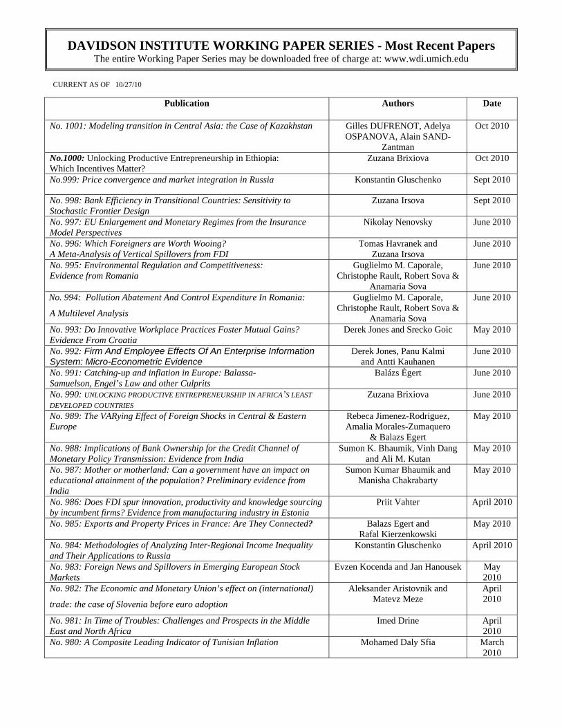
DAVIDSON INSTITUTE WORKING PAPER SERIES - Most Recent Papers The entire Working Paper Series may be downloaded free of charge at: www.wdi.umich.edu

CURRENT AS OF 10/27/10

Publication Authors Date

No. 1001: Modeling transition in Central Asia: the Case of Kazakhstan Gilles DUFRENOT, Adelya OSPANOVA, Alain SAND-

Zantman

Oct 2010

No.1000: Unlocking Productive Entrepreneurship in Ethiopia: Which Incentives Matter?

Zuzana Brixiova Oct 2010

No.999: Price convergence and market integration in Russia Konstantin Gluschenko Sept 2010

No. 998: Bank Efficiency in Transitional Countries: Sensitivity to Stochastic Frontier Design

Zuzana Irsova Sept 2010

No. 997: EU Enlargement and Monetary Regimes from the Insurance Model Perspectives

Nikolay Nenovsky June 2010

No. 996: Which Foreigners are Worth Wooing? A Meta-Analysis of Vertical Spillovers from FDI

Tomas Havranek and Zuzana Irsova

June 2010

No. 995: Environmental Regulation and Competitiveness: Evidence from Romania

Guglielmo M. Caporale, Christophe Rault, Robert Sova &

Anamaria Sova

June 2010

No. 994: Pollution Abatement And Control Expenditure In Romania:

A Multilevel Analysis

Guglielmo M. Caporale, Christophe Rault, Robert Sova &

Anamaria Sova

June 2010

No. 993: Do Innovative Workplace Practices Foster Mutual Gains? Evidence From Croatia

Derek Jones and Srecko Goic May 2010

No. 992: Firm And Employee Effects Of An Enterprise Information System: Micro-Econometric Evidence

Derek Jones, Panu Kalmi and Antti Kauhanen

June 2010

No. 991: Catching-up and inflation in Europe: Balassa-Samuelson, Engel’s Law and other Culprits Balázs Égert June 2010

No. 990: UNLOCKING PRODUCTIVE ENTREPRENEURSHIP IN AFRICA’S LEAST DEVELOPED COUNTRIES

Zuzana Brixiova June 2010

No. 989: The VARying Effect of Foreign Shocks in Central & Eastern Europe

Rebeca Jimenez-Rodriguez, Amalia Morales-Zumaquero

& Balazs Egert

May 2010

No. 988: Implications of Bank Ownership for the Credit Channel of Monetary Policy Transmission: Evidence from India

Sumon K. Bhaumik, Vinh Dang and Ali M. Kutan

May 2010

No. 987: Mother or motherland: Can a government have an impact on educational attainment of the population? Preliminary evidence from India

Sumon Kumar Bhaumik and Manisha Chakrabarty

May 2010

No. 986: Does FDI spur innovation, productivity and knowledge sourcing by incumbent firms? Evidence from manufacturing industry in Estonia

Priit Vahter April 2010

No. 985: Exports and Property Prices in France: Are They Connected? Balazs Egert and Rafal Kierzenkowski

May 2010

No. 984: Methodologies of Analyzing Inter-Regional Income Inequality and Their Applications to Russia

Konstantin Gluschenko April 2010

No. 983: Foreign News and Spillovers in Emerging European Stock Markets

Evzen Kocenda and Jan Hanousek May 2010

No. 982: The Economic and Monetary Union’s effect on (international)

trade: the case of Slovenia before euro adoption Aleksander Aristovnik and

Matevz Meze April 2010

No. 981: In Time of Troubles: Challenges and Prospects in the Middle East and North Africa

Imed Drine April 2010

No. 980: A Composite Leading Indicator of Tunisian Inflation Mohamed Daly Sfia March 2010