BearWorks BearWorks

MSU Graduate Theses

Spring 2021

Modeling the Growth and Establishment of Plantation and Modeling the Growth and Establishment of Plantation and

Converted Silvopasture Systems in the Missouri Ozarks Region Converted Silvopasture Systems in the Missouri Ozarks Region

Stewart James McCollum Missouri State University, sm1996@live.missouristate.edu

As with any intellectual project, the content and views expressed in this thesis may be

considered objectionable by some readers. However, this student-scholar’s work has been

judged to have academic value by the student’s thesis committee members trained in the

discipline. The content and views expressed in this thesis are those of the student-scholar and

are not endorsed by Missouri State University, its Graduate College, or its employees.

Follow this and additional works at: https://bearworks.missouristate.edu/theses

Part of the Agricultural Science Commons, and the Forest Management Commons

Recommended Citation Recommended Citation McCollum, Stewart James, "Modeling the Growth and Establishment of Plantation and Converted Silvopasture Systems in the Missouri Ozarks Region" (2021). MSU Graduate Theses. 3607. https://bearworks.missouristate.edu/theses/3607

This article or document was made available through BearWorks, the institutional repository of Missouri State University. The work contained in it may be protected by copyright and require permission of the copyright holder for reuse or redistribution. For more information, please contact BearWorks@library.missouristate.edu.

MODELING THE GROWTH AND ESTABLISHMENT OF PLANTATION AND

CONVERTED SILVOPASTURE SYSTEMS IN THE

MISSOURI OZARKS REGION

A Master’s Thesis

Presented to

The Graduate College of

Missouri State University

TEMPLATE

In Partial Fulfillment

Of the Requirements for the Degree

Master of Science, Plant Science

By

Stewart James McCollum

May 2021

ii

Copyright 2021 by Stewart James McCollum

iii

MODELING THE GROWTH AND ESTABLISHMENT OF PLANTATION AND

CONVERTED SILVOPASTURE SYSTEMS IN THE MISSOURI OZARKS REGION

Agriculture

Missouri State University, May 2021

Master of Science

Stewart James McCollum

ABSTRACT

The Missouri Ozarks are well known for high production in both timber products and cattle production. Most areas are also not well suited for many other agricultural practices such as row cropping, so forests and grazing lands dominate the landscapes. Such characteristics provide high potential for the agroforestry practice known as silvopasture. This study monitors the establishment of two different types of silvopasture systems, plantation and conversion types. In the plantation silvopasture, two cultivars of black walnut (Juglans nigra) were planted, Football and Kwikrop. Health and growth were monitored for those cultivars over the first year. The converted silvopasture consisted of a manually thinned upland forest area containing many different oak (Quercus) species as well as a few other hardwood species such as hickory (Carya) and ash (Fraxinus). The converted stand was monitored using an unmanned aerial system (UAS) equipped with a multispectral sensor. The multispectral imaging was used to create canopy height models as well as build models predicting seasonal climate stress variables such as leaf water potential and leaf chlorophyll content of the trees within the converted silvopasture system. The final seasonal climate stress models displayed relatively high prediction potential for important seasonal climate stress variables using remote-sensed data for different forest ecosystems in the Missouri Ozarks region. KEYWORDS: agroforestry, silvopasture, Ozarks, UAS, black walnut, hardwood

iv

MODELING THE GROWTH AND ESTABLISHMENT OF PLANTATION AND

CONVERTED SILVOPASTURE SYSTEMS IN THE

MISSOURI OZARKS REGION

By

Stewart James McCollum

A Master’s Thesis Submitted to the Graduate College

Of Missouri State University In Partial Fulfillment of the Requirements

For the Degree of Master of Science, Plant Science

May 2021 Approved: Michael Goerndt, Ph.D., Thesis Committee Chair

Will McClain, Ph.D., Committee Member

Melissa Bledsoe, Ph.D., Committee Member

Toby Dogwiler, Ph.D., Committee Member

Julie Masterson, Ph.D., Dean of the Graduate College In the interest of academic freedom and the principle of free speech, approval of this thesis indicates the format is acceptable and meets the academic criteria for the discipline as determined by the faculty that constitute the thesis committee. The content and views expressed in this thesis are those of the student-scholar and are not endorsed by Missouri State University, its Graduate College, or its employees.

v

ACKNOWLEDGEMENTS

I would like to thank the long list of people that have assisted me along this journey.

First, I would like to thank each and every person that encouraged me to continue my education

and pursue a master’s degree. Without their encouragement I would not be in this position today.

Next, all of the faculty members and students that helped with long days of data collection, this

would not have been possible without each and every one of you. Also, Dr. Toby Dogwiler for

all of his work with the remote sensed data collection and data post processing. Next, I would

like to thank my family for being such a wonderful support system through these years. This

would not have been possible without their support and encouragement. Lastly, and most

importantly, I would like to thank my advisor Dr. Michael Goerndt. Not only has he been an

amazing advisor, but a mentor in the field of forestry and all aspects of life. None of this would

have been possible without his support and guidance along this journey.

vi

TABLE OF CONTENTS Introduction Page 1

What is Silvopasture Page 2 Why Use Silvopasture Page 3 Black Walnut in Silvopasture Page 4 Remote Sensing in Forestry Page 5 Study Objectives Page 6

Materials and Methods Page 8 Study Site Page 8 Weather Data Page 8 Plantation Silvopasture Page 9 Conversion Silvopasture Page 12 Remote Sensed Data Collection Page 14 Canopy Height Model (CHM) Page 16 Seasonal Climate Stress Models Page 18 Study Limitations Page 20

Results Page 22 Weather Data Page 22 Plantation Silvopasture Page 23 Seasonal Climate Stress Models Page 25

July Models Page 25 September Models Page 25 Combined Seasonal Models Page 26

Discussion Page 30

Plantation Silvopasture Page 30 Mortality of Seedlings Page 30 Height and Diameter of Seedlings Page 31

Seasonal Climate Stress Models Page 32 Water Potential Page 32 Leaf Chlorophyll Page 34

Conclusions Page 36

References Page 38

Appendix Page 41

vii

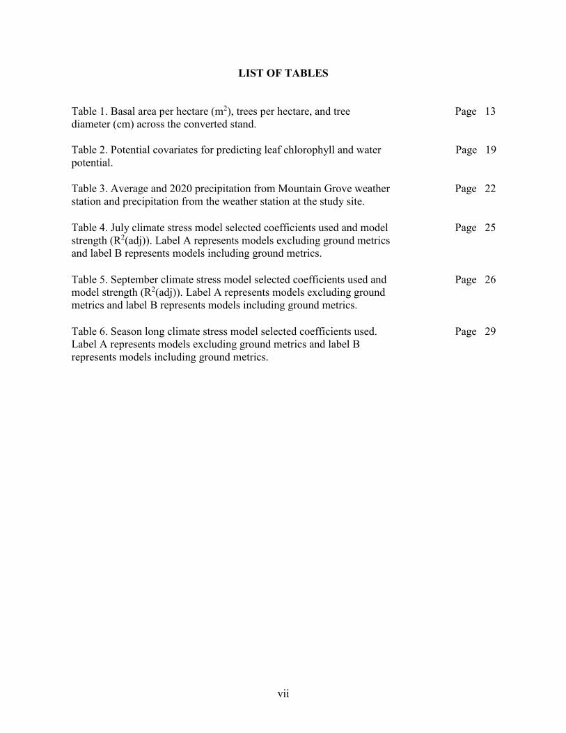
LIST OF TABLES

Table 1. Basal area per hectare (m2), trees per hectare, and tree diameter (cm) across the converted stand.

Page 13

Table 2. Potential covariates for predicting leaf chlorophyll and water potential.

Page 19

Table 3. Average and 2020 precipitation from Mountain Grove weather station and precipitation from the weather station at the study site.

Page 22

Table 4. July climate stress model selected coefficients used and model strength (R2(adj)). Label A represents models excluding ground metrics and label B represents models including ground metrics.

Page 25

Table 5. September climate stress model selected coefficients used and model strength (R2(adj)). Label A represents models excluding ground metrics and label B represents models including ground metrics.

Page 26

Table 6. Season long climate stress model selected coefficients used. Label A represents models excluding ground metrics and label B represents models including ground metrics.

Page 29

viii

LIST OF FIGURES

Figure 1. Map of Missouri State University’s Journagan Ranch property.

Page 8

Figure 2. Walnut plantation silvopasture layout and design. Page 11 Figure 3. Layout of the .04 hectare plots and the nested sub-plot structure.

Page 13

Figure 4. Reflectance bands captured by the Micasense RedEdge-M camera and common reflectance of vegetation (Micasense 2018).

Page 15

Figure 5. Example of the highest points (left), lowest or ground points (center), and the difference of the two creating a CHM (right).

Page 17

Figure 6. Crown polygon from crown delineation. Page 18 Figure 7. Mortality (n=36) and top kill rates of football (top kill n=27) and Kwikrop (top kill n=24) cultivars.

Page 24

Figure 8. Mean ± SE of height and diameter growth of football (height n=18, diameter n=22) and Kwikrop (height n=4, diameter n=21) cultivars.

Page 24

Figure 9. Residual plots for all mixed models. Page 28

1

INTRODUCTION

The Ozark Highland Ecoregion is approximately 108,332 square kilometers (10,833,200

hectares) primarily in southern Missouri, but also in northern Arkansas, southeastern Kansas, and

northeastern Oklahoma (Karstensen 2010). Of that land, a survey in 2000 stated that 56.2% and

36.8% of the land use was forest and agriculture, respectively (Karstensen 2010). Missouri is

known for its abundant forest resources with nearly 6 million hectares of forest land across the

state (Leatherberry and Treiman 2002). This allows Missouri to be a leading producer in a

variety of forest products including wood pallets, charcoal, oak barrels, and walnut products

(Leatherberry and Treiman 2002). However, Missouri is better known for its cattle production. In

2017, Missouri ranked second among all states in beef cattle production, as well as second in

cow-calf production in 2018 (USDA 2018). These two commodities provide great opportunity

for the use of the agroforestry practice known as silvopasture.

As the world population continues to increase, the need for food also increases. This

leads to an increased demand of agricultural lands. The rocky slopes of the Ozarks are not well

suited for many crop species, so grazing lands dominate the landscapes. Searcy County of

northern Arkansas has been experiencing vast amounts deforestation for the expansion of

pastures (Wall 1996). “The increase in cattle production is directly linked to increased

deforestation,” states Wall (1996). Not only has northern Arkansas experienced deforestation, the

entire Ozark Highland Ecoregion has also been subject. In a land use study of the Ozark

Highland Ecoregion from 1973-2000, the most common type of land use conversion was from

forest to agriculture (Karstensen 2010). The percent of forest cover across the region decreased

2.3% while the agricultural land use increased 1.7% over the study period (Karstensen 2010).

2

Proper education of silvopasture could promote its use and potentially slow the crisis of

deforestation across the region.

What is Silvopasture

Silvopasture is the intentional combination of trees and forage in the same location. This

can be accomplished by the establishment of trees into a pasture or the establishment of a forage

into managed forest stands (Klopfenstein et al. 1997, Garrett et al. 2004, Hamilton 2008).

Silvopasture must be intensively managed to maintain productivity (Jose et al. 2019).

Silvopasture, as well as other types of agroforestry practices, have been used around the world

for centuries, commonly in areas with subsistence farming (Nair 2011). However, modern

agroforestry began primarily in the tropics as a way to combat tropical deforestation, soil

degradation, and biodiversity decline (Nair 2011). Then, around the 1980s and 1990s,

agroforestry practices became more recognized and used in many developing countries (Nair

2011).

To receive the potential benefits of silvopasture, it is important to understand the

difference between silvopasture and forest grazing or woodland grazing. With the idea of it being

beneficial, farmers will often times allow livestock to graze within woodlands, even if pasture is

available (DeWitt 1989). This is different from silvopasture because proper management has not

been applied with concerns for trees and/or livestock (Orefice and Carroll 2017). In a natural

forest or woodland, it could take up to 40 hectares to provide the equivalent forage of one hectare

of pasture, leading to lower weight gains and poorer quality meat in cattle (DeWitt 1989).

Without proper management, many plants can be present in a woodland environment that may be

harmful to livestock. Some of these being black cherry and poison ivy, both being common in

3

Missouri woodlands (DeWitt 1989). Soil erosion can also be high in a grazed woodland due to

less low growing vegetation than in a silvopasture (DeWitt 1989). Without proper management

to create a silvopasture, the cost of woodland grazing can easily outweigh the benefits.

Why Use Silvopasture

Silvopasture is often used to provide multiple sources of income from one piece of land.

However, the benefits go far beyond economics. Trees can benefit from grazing as grass

competition is reduced. Grazing also helps control weeds and brush that potentially have

negative impacts on tree growth and quality. Grazing livestock allows nutrients to be recycled

back into the soil through manure and urine reducing fertilization costs (Klopfenstein et al.

1997). Trees can also recycle nutrients by absorbing nutrients below the rooting zone of the

forage and applying them back to the surface through leaf litter (Buresh et al. 2004).

Furthermore, forage typically has lower fiber content and is more digestible to the livestock

when grown in an environment with trees. Livestock also benefit from the shade of trees for less

heat stress in summer and trees as a windbreak can reduce wind-chill of livestock in winter

(Klopfenstein et al. 1997). With a properly managed practice, silvopasture can be successful and

have many benefits (Orefice and Carroll 2017).

Farmers however, are not the only one that reap the benefits of silvopasture. Silvopasture

as well as other agroforestry practices have proven to benefit the environment in a variety of

ways (Nair 2011). Trees are able to take up nutrients that have leached below the forage root

zone that would otherwise leach into ground water or surface water causing pollution (Michel et

al. 2007). Carbon sequestration is another huge benefit. Silvopastures have a greater potential to

capture and store more carbon than a traditional pasture (Nair 2011). Improved water quality,

4

slowing of climate change through carbon sequestration, and higher biodiversity are important

benefits of silvopastures (Nair 2011).

Black Walnut in Silvopasture

Black walnut (Juglans nigra) is a very common species chosen for agroforestry practices

in Missouri because of its high valued wood and nut crop (Garrett et al. 1991, Garrett et al.

1996), and Missouri is a well-known producer for both the wood and nut crop of black walnut.

Aside from being a profitable crop, some of its traits pair well with many crops or forage species.

The growth period of black walnut is about 90-135 days and is one of the shortest for tree species

(Garrett et al 1996). The extra time in the spring and fall without leaves on the trees is important

for understory growth of some forage species. Not only is the growing season shorter, but also

the crowns of black walnut are fairly sparse and allow a sufficient amount of light through to the

ground for successful growth of many cool-season grasses (Garrett et al 1996).

Black walnut, however, can draw some concerns when it comes to using it in agroforestry

practices. This is because of the allelopathic chemical juglone, produced in the roots of black

walnut (Funt and Martin 1999, Jose and Holzmueller 2008). Effects of juglone have been studied

on many different species, with a list of plants that are susceptible continuing to grow. However,

select species have been found to be useful in agroforestry practices paired with black walnut

(Scott and Sullivan 2007). Most grass species fall within this category or have been observed

under black walnut (Funt and Martin 1999), suggesting good potential for black walnut in

silvopastoral systems.

5

Remote Sensing in Forestry

Remote sensed data is a term that is being used more frequently in many different fields

of science, including forestry and agriculture. With increases in technology, satellite imaging as

well as unmanned aerial systems (UAS) have become much more popular for forest monitoring

over the past few decades (Grenzdörffer et al. 2008, Tang and Shao 2015, Banu et al. 2016).

Arial photography has been used as far back as the 1860s, and increased in use with the

introduction of Earth Orbiting satellites around 1960 (Tang and Shao 2015). Since the 1970s,

more satellites began to be equipped with digital sensors and became more available for civil

applications (Tang and Shao 2015). Since then satellite imaging has become more popular but

with limited spectral resolution (Banu et al. 2016). UASs however have the ability to provide

much higher spectral resolution when needed (Banu et al. 2016). UASs have also become more

accessible and affordable over the years, increasing the popularity of UAS remote sensed data

(Mahjan and Bundel 2016).

A wide variety of forest data can be obtained from the use of multiple different sensors

equipped on the UAS. These can be as simple as mapping forest boundaries and as specific as

estimated volume or trees per hectare. LiDAR (Light Detection and Ranging) sensors are a

common tool used to determine tree height and canopy coverage (Tang and Shao 2015, Banu et

al 2016). LiDAR is a method to measure height by using a laser pulse emitted from the UAS to

determine distance from the object below the UAS. The time it takes for the laser pulse to return

determines the distance (Lefsky et al. 2002). This is done repeatedly over an area of the earth’s

surface providing a model of tree canopy dynamics. Another popular sensor would be

multispectral and hyper spectral sensors (Tang and Shao 2015). These sensors are able to collect

light wavelengths outside of the visible light spectrum (red, green, and blue). Using the spectral

6

reflectance in these wavelengths allows us to identify differences in species and stressed plants

from insects, diseases, or other causes (Minarik and Langhammer 2016, Dash et al. 2017). This

is an important tool in forest management as it allows ease of monitoring, evaluating, and

predicting different aspects of the forest.

Study Objectives

The primary goal of this study is to build the capacity for future research. Future research

providing information regarding economics, establishment, sustainability, and production

potential of silvopasture systems. In light of this goal, the initial objectives of this study were to

establish two different functioning silvopasture systems using planting and thinning methods.

Planting silvopasture consists of planting a desired tree species or group of multiple

species into a pre-existing grassland. Planting density and spacing would follow a plan

determined by both tree species and forage species that will be grown as well as the long term

goals of the user. This method takes longer for trees to reach a size that can attribute to the

benefits of silvopasture.

Conversely, converting timberland or forest to silvopasture consists of selecting desirable

trees to keep and removing the remaining trees and shrubs using thinning methods and then

establishing a desirable forage species. Density and spacing will be much more variable

depending on tree species, tree size, and initial tree spacing within the forest. The variable

spacing of trees can make management more challenging, however, the silvopasture system is

ready immediately following successful forage establishment.

Additionally, remote sensing was used to create canopy height models and climate stress

models of the conversion silvopasture system. The stress models were created to evaluate the

7

effects of climate changes and stressors throughout the year and build models to predict plant

stress from remote sensed data. These models can be used not only to predict seasonal climate

stress in silvopasture systems but also to potentially model and predict climate stress in addition

to other biophysical attributes such as species composition, crown structure, and disease presence

in other forest ecosystems.

8

MATERIALS AND METHODS

Study Site

This research was conducted at Missouri State University’s (MSU) Journagan Ranch

property in Douglas County of south central Missouri. Journagan Ranch is a 1335 hectare ranch

that houses the largest pure-bred Hereford heard in the state of Missouri. It also consists of very

diverse landscapes and soil types (Figure 1). This area falls centrally within the Ozark Highland

Ecoregion. The specific site consisted of two study areas: 1) plantation silvopasture, and 2)

existing forest stand thinned for silvopasture.

Figure 1. Map of Missouri State University’s Journagan Ranch property.

Weather Data

A weather station was set up toward the center of both of the silvopasture study areas to

monitor specific site weather for years to come. Metrics recorded over the 2020 growing season

included: rainfall, air temperature, soil temperature, water content, relative humidity, wind

direction, wind speed, and evapotranspiration. These stations were set up and began recording

9

data on July 1, 2020. The University of Missouri weather station located in Mountain Gove, MO

was used for long term weather metrics for the local vicinity. This weather station is located 15

kilometers north of the study area. Annual and monthly averages of rainfall and air temperature

were calculated based upon data from 2008 to 2020.

Plantation Silvopasture

The newly established plantation silvopasture measures 219.45 m by 73.15 m. This site

was planted with two cultivars of black walnut: Football and Kwikrop. Walnuts from these two

cultivars were collected from the University of Missouri Southwest Research Center in Mt.

Vernon, MO. Following collection, the black walnuts were placed in five gallon buckets with

holes drilled for water drainage and buried in the soil for stratification over the winter of

2018/19. Following stratification, the black walnuts were planted into raised planting beds at

MSU’s Shealy Farm near Fair Grove, MO. The planting beds were roughly 25 cm tall with the

bottom four to five cm filled with small gravel to allow drainage. The remainder of the bed was

filled with topsoil. The black walnuts germinated and grew in the beds through the year of 2019.

A surplus of black walnut seedlings were grown to provide selection of better individuals as well

as to have replacements for following years. On December 18, 2019, seedlings appearing healthy

with large healthy appearing root systems were collected. The selected individuals were planted

at the Journagan Ranch study site the following day (December 19, 2019). The plantation design

is comprised of 72 trees, including 36 of each cultivar. Trees were planted at a spacing of 12.2 m

within rows and 18.3 m between rows. Tree spacing was chosen to allow sufficient light for

forage growth and crown expansion for nut production. A mature walnut tree crown, when open-

grown in a nut plantation setting, will get to approximately 12x12 m crown area on average

10

(Garrett et al. 1996). The selected spacing between trees will also facilitate the movement and

operation of heavy farm equipment in future years. The seedlings were planted into 12 rows of

six trees across the pasture. The pasture was divided into three equal blocks, each containing four

rows of trees (two of each cultivar). The cultivars were randomly assigned to rows in each block

(Figure 2). Competition from grass is a big limiting factor when it comes to seedling growth

(Hamilton 2008, Houx III et al. 2013). An ideal weed-free zone is around a 0.6-0.9 m radius

around established seedlings (Hamilton 2008), with studies finding that tree growth rates stop

increasing with a weed-free zone radius greater than 1.2 m (Houx III et al. 2013). In this study, a

2.5% concentration of glyphosate was applied in a 0.75 m radius circle around each planting

location for site preparation in the fall of 2019. An additional application (same concentration)

was done the third week of July 2020 to maintain the weed-free zone. A wire cage was placed

around each seedling to prevent wildlife predation and damage. The cages were made from

welded wire and were 1.5 m tall and 30 cm in diameter. Many of the seedlings were infected

with Gnomonia leptostyla, a fungal anthracnose that effects walnut trees, during 2020. Daconil

fungicide was applied the third week of July 2020 to combat the anthracnose.

Measurements of black walnut seedlings for the first year’s growth at the Journagan

ranch site included survival rate of the cultivars, height growth, and diameter growth. Height

growth was measured at planting (before growth began) and at the end of the growing season in

centimeters. Diameter growth was taken in millimeters using electronic calipers at initial

planting and at the end of the growing season at 20.3 cm above the ground. The measurement

height of 20.3 cm for diameter was chosen as a logical standard based on the average initial

height of seedlings and the fact that a diameter at breast height (dbh) measurement was not

11

possible for seedlings. At the end of the growing season, the mortality and growth rates of

surviving trees were measured using the same standards as the initial measurements.

Figure 2. Walnut plantation silvopasture layout and design.

Health was assessed for the trees throughout the growing season and those that did not

survive or were in poor condition were taken note of for replacement. In January of 2021, the

individuals that did not survive were replaced with two new seedlings from the remaining

12

seedlings in the Shealy Farm germination beds so they are the same age as the others within the

silvopasture plantation. The individuals that were in poor condition but not dead were retained

but an additional seedling was planted immediately next to the original tree and marked as a

back-up. The locations with multiple seedlings will be re-evaluated in the future years and the

stronger seedling will be kept.

Conversion Silvopasture

The converted forest stand was an uneven aged forest stand that was thinned for

silvopasture. The area measures about two hectares and the dominant and codominant species

composition of the stand consisted primarily of White oak (Quercus alba), Post oak (Quercus

stellata), Red oak (Quercus rubra), Black oak (Quercus velutina), Hickory (Carya spp.), with

the occasional Ash (Fraxinus spp.), and Black Walnut (Juglans nigra). Before thinning, a forest

inventory was taken using eight systematically spaced .02 hectare circular plots. In each plot

every tree was tallied, identified by species, given a crown classification, and measured for DBH.

The stand had an average of 19.2 square m of basal area per hectare, an average of 389 trees per

hectare, and a mean diameter of 23.1 cm (Table 1). The stand was then thinned with the goal to

remove 50% of the crown cover (Garrett et al. 2004). This would be reducing the stocking level

to about 30% stocked according to the Gingrich stocking chart (Gingrich 1967). 30% stocking

allows about 50% light transmittance (Sander 1979) which is recommended for maximum cool

season forage growth (Gardner et al. 1985). Following the thin, 18 .04 hectare circular plots were

set up for a follow up inventory and repeat measurements in the future (Figure 3). Every tree

within the plot was tallied, identified, and diameter was measured. The average basal area after

the thin was 9.3 square m per hectare, there was an average of 110 trees per hectare, and the

13

mean diameter was 32 cm (Table 1). Along with the basic inventory measurements, following

the thin crown width and crown density were collected and will be collected annually to monitor

growth over time.

Table 1. Basal area per hectare (m2), trees per hectare, and tree diameter (cm) across the converted stand. BA/H TPH DBH Before Thin Mean 19.2 389 23.1 CV % 11.6 88 106.9 Min 10.1 198 10.2 Max 37.3 593 49.2 After Thin Mean 9.3 110 32 CV % 10.5 118 57.4 Min 3.4 25 17 Max 17.4 222 54.4

Figure 3. Layout of the .04 hectare plots and the nested sub-plot structure.

14

Other measurements were taken at different times during the growing season to

correspond with the remote sensed data collection. These dates were, July 8 and September 20.

For those dates, in each of the 18 .04 hectare plots the following measurements were taken at the

plot center and halfway between the plot center and boundary in each cardinal direction for five

total measurements: Light intensity, soil moisture, and soil temperature (Figure 3). Those values

were then used to calculate a plot-level mean estimate. Light intensity was taken using an

Apogee Instruments MQ-306 Line Quantum PAR (Photosynthetically Active Radiation) sensor.

Soil moisture was taken using a Campbell Scientific® HydroSense II handheld soil moisture

meter that gives volumetric water content in percent. Soil Temperature was taken using a

SpotOn® digital temperature probe witch gives values in degrees Fahrenheit. Leaf chlorophyll

and water potential were also measured on both dates. For these measurements, one tree per plot

was selected and marked to be used for resampling throughout the years. A leaf sample was

collected from as high as possible in the tree crown using a shotgun to shoot down a cluster of

leaves. An Apogee Instruments MC-100 chlorophyll meter was used to measure chlorophyll

concentration of the leaf in µmol m-2. An average value of leaf chlorophyll content was recorded

from eight measurements on one leaf. Water potential was measured for one leaf per plot using

the Model 600 pressure chamber instrument by PMS Instrument Company. For consistency, an

oak tree was selected for the leaf measurements in every plot except for plot three and plot nine,

where no oak was present so a hickory and ash were chosen respectively.

Remote Sensed Data Collection

Remote sensed data was collected using a phantom 4 professional unmanned aerial

system (UAS) by DJI. This UAS is known as a quadcopter UAS meaning it is controlled using

15

four rotors to control flight. This is different than a fixed-wing UAS which resembles an

airplane. The quadcopter UAS require much less space to take off and land opposed to the fixed

wing style (Mahjan and Bundel 2016). The UAS was flown on the two dates from above during

the 2020 growing season: July 8 and September 20. For each of these dates RGB data was

collected as well as Multispectral data that includes RGB bands, Red Edge and Near-infrared

data (Figure 4). Multispectral imaging was collected using a Micasense RedEdge-M sensor.

Data collection was performed at mid-day (10 AM – 2 PM) on each flight to minimize

shadows and maximize consistent light transmittance. For both flight dates the UAS was flown

at a height of 85 m above the ground for both RGB and Mulitspectral data collection. Ground

resolution of the RGB photos was set to 2.3 cm for both flights while the Multispectral resolution

was 5.9 cm for both. Flight path and capture speed were established to provide 80% forward and

side overlap to the next picture, allowing each location on the ground to be captured by

approximately 25 images.

Figure 4. Reflectance bands captured by the Micasense RedEdge-M camera and common reflectance of vegetation (Micasense 2018)

16

Canopy Height Model (CHM)

Following the UAS flights, data was post processed using the Agisoft Metashape

Photoscan program. For all flights, the Unmanned Aircraft Systems Data Post-Processing

workflow was primarily followed (USGS 2017). Two different digital elevation models (DEM)

were created using the program. One is elevation of the highest points in each pixel, which can

represent the upper canopy of trees, peaks of higher elevation bare ground, birds, or other objects

above typical ground elevation. The other is the lowest point in each pixel, which can represent

ground level, but can also be influenced by low-lying vegetation and other objects on the ground.

Using these two DEMs a raster set that displays values of the height of the vegetation by

subtracting the ground only DEM from the highest point DEM in Esri ArcMAP was created

(Figure 5). This is considered a form of canopy height model (CHM), such as the typical canopy

representation often calculated using LiDAR point cloud data. The CHM was then used to

delineate tree crowns within the converted silvopasture. To facilitate tree crown delineation, only

pixels with a raster pixel value greater than 6 m were considered, as lower values often represent

low-lying vegetation and ground variability. Finally, polygons were created around conspicuous

clusters of retained pixels to represent tree crown edge (Figure 6) (Appendix).

17

Figure 5. Example of the highest points (left), lowest or ground points (center), and the difference of the two creating a CHM (right).

18

Figure 6. Crown polygon from crown delineation.

Seasonal Climate Stress Models

Stress models were created using a combination of the UAS data and ground data. The

models were built to predict the water potential and leaf chlorophyll for trees within the

converted silvopasture. A model was created for each flight, as well as a combined prediction

model for the entire season. The potential covariates for the models included all reflectance

values collected from the UAS, multiple vegetative indices derived from the original reflectance

values, soil moisture, and soil temperature (Table 2). Zonal statistics in ArcMap was used to

extract a mean value for each of the multispectral covariates in each of the .04 hectare plots.

Mean values were calculated manually for soil moisture and soil temperature in each plot. For

19

the reflectance values and vegetative indices, the canopy model was used to extract values that

represent tree crown only. Two different models were created for each flight date and the

combined season model, one using all covariates listed above, and the other excluding soil

moisture and soil temperature as potential covariates. This was done to assess the statistical

importance of soil moisture and temperature on predicting water potential and leaf chlorophyll.

Table 2. Potential covariates for predicting leaf chlorophyll and water potential.

Climate stress models were created using the lm and lme toolpacks in R statistical

software. Multiple linear regression was used to create both the flight-specific and seasonal

models with all covariates listed above. Stepwise selection was used for each flight-specific

model to determine which covariates resulted in the strongest model fit for that specific data set.

Final flight-specific models were then created using only the ideal covariates selected through

stepwise regression. A linear mixed model was used to create the combined seasonal model

using both flight dates. Linear mixed models were used instead of ordinary least squares (OLS)

regression due to the intrinsic use of multiple flight times. This essentially represents a case of

repeated measures, as the same observations (plots) are remeasured for each flight time.

Description Variable Multispectral Bands Blue

Green Red Red Edge NIR

Multispectral Indices NDVI GNDVI RENDVI NLI

Ground Measurements Soil Moisture Soil Temperature

20

Therefore, the linear mixed models included flight time as a random variable with all other

covariates fixed. The stepwise selection method was used again to determine the strongest

covariates for the mixed models.

Study Limitations

For the plantation silvopasture, the sample size was fairly small with only 36

individuals per cultivar. A much larger sample would be ideal, but this specific area did not

allow for a more spatially extensive design. Tree planting by hand was another limitation.

Multiple people took part in the tree planting operation, in part to provide opportunities for field

experience to students. To be more consistent and avoid potential human errors, a mechanical

planter with two operators could have benefitted the study, though such precise spacing would

have been more challenging. Uncontrollable weather is also a limitation to the study. Without

easy access to irrigation, some aspects of success are ultimately dependent upon weather.

In the converted stand, the primary limitation is tree spacing. Because this area was a

naturally grown forest, trees of all sizes were spaced randomly across the entire stand. When

selecting dominant and co-dominant trees to retain, it was impossible to keep consistent spacing.

Size of the trees were also a limitation for the same reasons. Trees with larger canopies would

need more spacing to other trees for adequate light transmittance for forage growth. These

factors made each plot different from one another in the aspects of canopy coverage, trees per

hectare, and light transmittance. While considered a limitation, the aforementioned issues with

spacing are not unusual for mixed hardwood forests in the Ozarks region. Variations in tree size

and natural clustering of species across the landscape are challenges that every forester and

landowner have to contend with in any forest management scenario.

21

Lastly, with only one growing season of data collection complete, the short duration of

the study is a major limitation. In addition, most data collection came later in the growing season

verses throughout the entire growing season. Continual data collection should greatly increase

this study’s potential.

22

RESULTS

Weather Data

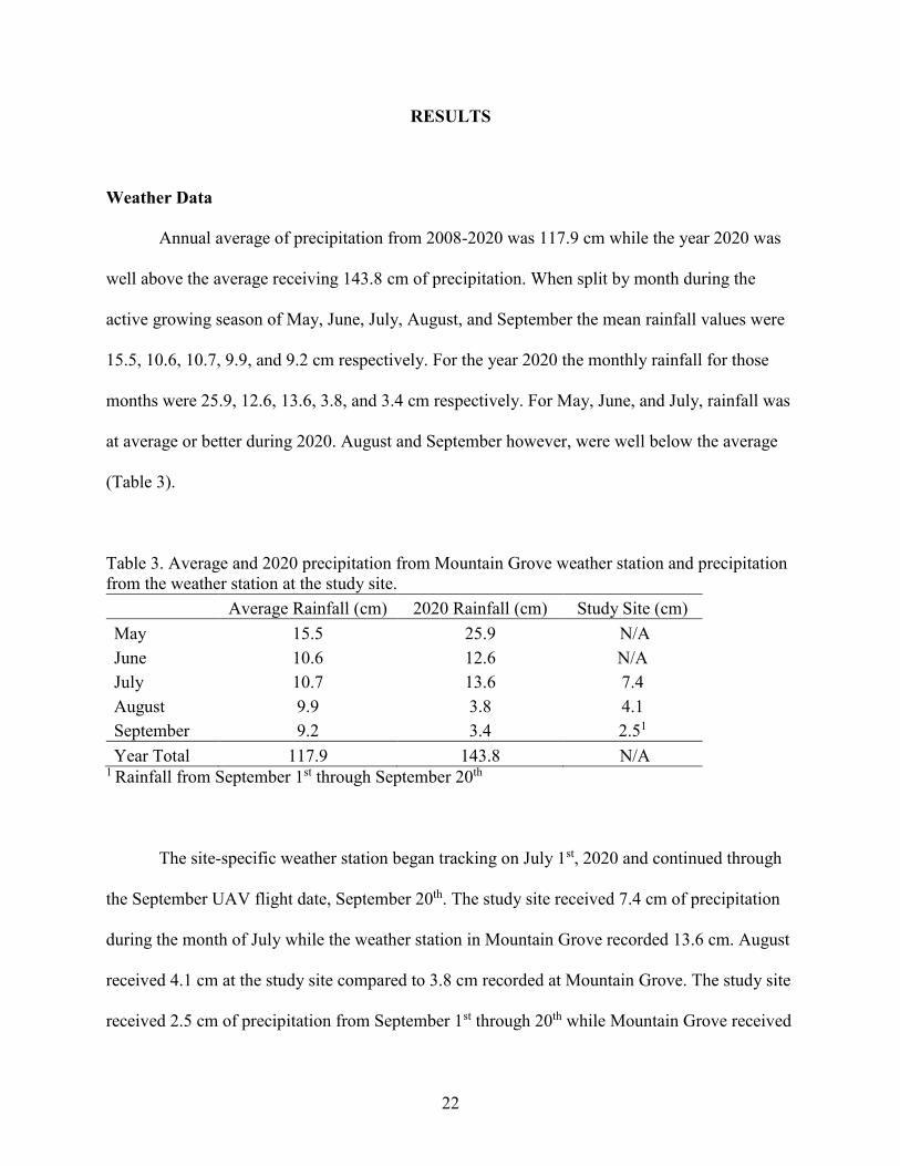
Annual average of precipitation from 2008-2020 was 117.9 cm while the year 2020 was

well above the average receiving 143.8 cm of precipitation. When split by month during the

active growing season of May, June, July, August, and September the mean rainfall values were

15.5, 10.6, 10.7, 9.9, and 9.2 cm respectively. For the year 2020 the monthly rainfall for those

months were 25.9, 12.6, 13.6, 3.8, and 3.4 cm respectively. For May, June, and July, rainfall was

at average or better during 2020. August and September however, were well below the average

(Table 3).

Table 3. Average and 2020 precipitation from Mountain Grove weather station and precipitation from the weather station at the study site. Average Rainfall (cm) 2020 Rainfall (cm) Study Site (cm) May 15.5 25.9 N/A June 10.6 12.6 N/A July 10.7 13.6 7.4 August 9.9 3.8 4.1 September 9.2 3.4 2.51

Year Total 117.9 143.8 N/A 1 Rainfall from September 1st through September 20th

The site-specific weather station began tracking on July 1st, 2020 and continued through

the September UAV flight date, September 20th. The study site received 7.4 cm of precipitation

during the month of July while the weather station in Mountain Grove recorded 13.6 cm. August

received 4.1 cm at the study site compared to 3.8 cm recorded at Mountain Grove. The study site

received 2.5 cm of precipitation from September 1st through 20th while Mountain Grove received

23

1.5 cm during that time frame and 3.4 cm for the entire month of September. The comparatively

low precipitation for the months of August and September is an important factor to remember

with regard to the discussion of climate stress model results in the next section.

Plantation Silvopasture

Mortality was recorded for both cultivars across the plantation. The Kwikrop cultivar had

a slightly higher mortality rate of 33.3% compared to a 25% mortality rate for the Football

cultivar (Figure 7). In addition to mortality, many individuals experienced top kill where the

terminal bud did not survive but a lateral bud did. Of the surviving seedlings, 33.3% of the

Football cultivar suffered from top kill and 83.3% of the Kwikrop cultivar experienced top kill

(Figure 7). Height growth was calculated from the surviving individuals that did not die or

experience top kill. Based on a simple t-test, there was no significant difference in height growth

between the cultivars. Football and Kwikrop had a mean height growth of 2.11 centimeters and

1.83 centimeters respectively (Figure 8). The five Football seedlings and three Kwikrop

seedlings with negative height growth were excluded when calculating mean height growth. We

again saw no significant difference between the two cultivars. Football and Kwikrop both had a

mean diameter growth of .35 mm (Figure 8).

24

Figure 7. Mortality (n=36) and top kill rates of football (top kill n=27) and Kwikrop (top kill n=24) cultivars.

Figure 8. Mean ± SE of height and diameter growth of football (height n=18, diameter n=22) and Kwikrop (height n=4, diameter n=21) cultivars.

0

10

20

30

40

50

60

70

80

90

Mortality Top Kill (of surviving seedlings)

Per

cen

tSuccess of Seedlings

Football Kwikrop

0.0

0.5

1.0

1.5

2.0

2.5

3.0

Football Kwikrop

Cen

tim

eter

s

Mean Height Growth

0

0.05

0.1

0.15

0.2

0.25

0.3

0.35

0.4

0.45

Football Kwikrop

Mill

imet

ers

Mean Diameter Growth

25

Seasonal Climate Stress Models

July Models. For July, the model predicting water potential was very strong for both

inclusion and exclusion of ground-measured soil moisture and soil temperature. Without

inclusion of ground metrics, this model had an adjusted R-squared value of 71.3%. When the

ground metrics of soil moisture and soil temperature were included, the adjusted R-squared value

increased to 79.2%. The same covariates were chosen in both models with the addition of soil

moisture in the ground metrics model (Table 4). For the model predicting chlorophyll in July, the

adjusted R-squared values were 29.5% and 20.6% for models excluding ground metrics and

including ground metrics respectively (Table 4).

Table 4. July climate stress model selected coefficients used and model strength (R2(adj)). Label A represents models excluding ground metrics and label B represents models including ground metrics. Coefficient Water Potential (Bars) Chlorophyll (µmol/m²) A B A B Intercept 0.0008* 0.0028* 0.1785 0.3131 Blue 0.0003* 0.0018* 0.2326 Green 0.0086* 0.0851 0.2074 Red 0.0534 0.1135 0.1635 Red Edge 0.0004* 0.0017* 0.1084 NIR 0.0001* 0.0006* 0.1435 NDVI 0.0006* 0.0018* GNDVI 0.0112* RENDVI 0.0444* 0.0592 NLI 0.1791 0.3142 Soil Moisture 0.046* 0.2525 Soil Temperature 0.1979 R²(adj), % 71.3 79.2 29.5 20.6

*Coefficients that show significance (p-value <0.05)

September Models. In September, both models predicting water potential used the same

three covariates with an adjusted R-squared value of 3.3% (Table 5). The model that included

26

soil moisture and soil temperature as potential covariates did not actually use these metrics, as

they did not increase model fit strength based on the stepwise regression procedure. The models

predicting chlorophyll had adjusted R-squared values of 46.5% and 52.2% for exclusion of

ground metrics and inclusion of ground metrics models respectively (Table 5). The model

excluding ground metrics used most of the covariates while the ground metrics model used all

covariates except for soil moisture.

Table 5. September climate stress model selected coefficients used and model strength (R2(adj)). Label A represents models excluding ground metrics and label B represents models including ground metrics. Coefficient Water Potential (Bars) Chlorophyll (µmol/m²) A B A B Intercept 0.112 0.112 0.0011* 0.3867 Blue 0.108 0.108 0.3815 Green 0.0047* 0.0877 Red 0.0196* 0.133 Red Edge 0.0405* 0.144 NIR 0.0018* 0.0026* NDVI 0.111 0.111 0.0147* 0.0583 GNDVI 0.0042* 0.1041 RENDVI 0.2032 NLI 0.112 0.112 0.3861 Soil Moisture Soil Temperature 0.084 R²(adj), % 3.3 3.3 46.5 52.2

*Coefficients that show significance (p-value <0.05)

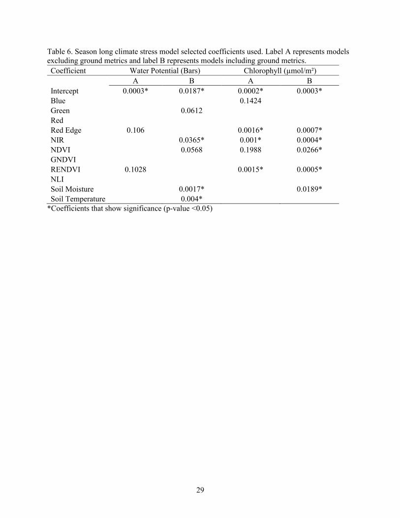
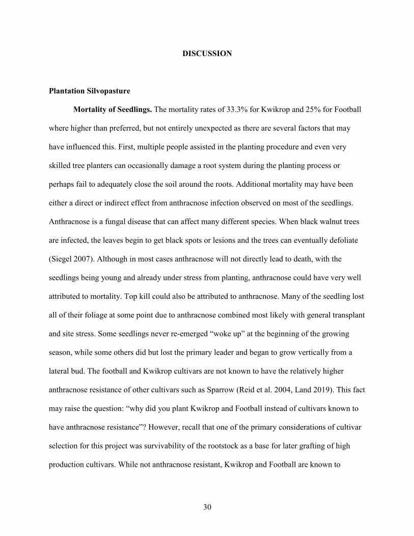
Combined Seasonal Models. The mixed model strength was evaluated using residual

plots as R does not provide adjusted R-squared values in a mixed model. Additionally, residual

plots are extremely useful, as they allow direct comparison of the prediction potential between

the various models and allow for assessment of regression assumptions (Figure 9). The

chlorophyll models used the same covariates with the exception of the ground data not using the

27

blue band and including soil moisture. The water potential models used different covariates for

each one (Table 6). Both water potential and chlorophyll models utilized a higher number of

significant covariates when including the ground data indicating stronger models.

Figure 9 illustrates that both water potential and chlorophyll models had slightly tighter

residuals when ground-based metrics of soil moisture and soil temperature were included in the

model. This feature indicates a relatively higher model fit when compared to the models that

excluded the ground-based variables. Also, it was determined by assessing the residual plots that

none of the models display any conspicuous issues with heteroskedasticity, non-linearity or

inappropriate scaling of values. It is also worth pointing out that there was an obvious trend

between the flight-specific models and seasonal climate stress models for both the Red-Edge and

NIR covariates to be significant, particularly for predicting changes in chlorophyll. This factor

will be expanded upon further in the discussion section.

28

Figure 9. Residual plots for all mixed models.

-15

-10

-5

0

5

10

15

20 22 24 26 28 30 32 34Res

idu

als

Predicted Value

Water Potential Excluding Ground Data

-10

-8

-6

-4

-2

0

2

4

6

8

10

6 8 10 12 14 16 18 20 22Res

idu

als

Predicted Values

Chlorophyll Excluding Ground Data

-15

-10

-5

0

5

10

15

20 22 24 26 28 30 32 34 36Res

idu

als

Predicted Values

Water Potential Including Ground Data

-10

-8

-6

-4

-2

0

2

4

6

8

10

6 8 10 12 14 16 18 20 22Res

idu

als

Predicted Values

Chlorophyll Including Ground Data

29

Table 6. Season long climate stress model selected coefficients used. Label A represents models excluding ground metrics and label B represents models including ground metrics. Coefficient Water Potential (Bars) Chlorophyll (µmol/m²) A B A B Intercept 0.0003* 0.0187* 0.0002* 0.0003* Blue 0.1424 Green 0.0612 Red Red Edge 0.106 0.0016* 0.0007* NIR 0.0365* 0.001* 0.0004* NDVI 0.0568 0.1988 0.0266* GNDVI RENDVI 0.1028 0.0015* 0.0005* NLI Soil Moisture 0.0017* 0.0189* Soil Temperature 0.004*

*Coefficients that show significance (p-value <0.05)

30

DISCUSSION

Plantation Silvopasture

Mortality of Seedlings. The mortality rates of 33.3% for Kwikrop and 25% for Football

where higher than preferred, but not entirely unexpected as there are several factors that may

have influenced this. First, multiple people assisted in the planting procedure and even very

skilled tree planters can occasionally damage a root system during the planting process or

perhaps fail to adequately close the soil around the roots. Additional mortality may have been

either a direct or indirect effect from anthracnose infection observed on most of the seedlings.

Anthracnose is a fungal disease that can affect many different species. When black walnut trees

are infected, the leaves begin to get black spots or lesions and the trees can eventually defoliate

(Siegel 2007). Although in most cases anthracnose will not directly lead to death, with the

seedlings being young and already under stress from planting, anthracnose could have very well

attributed to mortality. Top kill could also be attributed to anthracnose. Many of the seedling lost

all of their foliage at some point due to anthracnose combined most likely with general transplant

and site stress. Some seedlings never re-emerged “woke up” at the beginning of the growing

season, while some others did but lost the primary leader and began to grow vertically from a

lateral bud. The football and Kwikrop cultivars are not known to have the relatively higher

anthracnose resistance of other cultivars such as Sparrow (Reid et al. 2004, Land 2019). This fact

may raise the question: “why did you plant Kwikrop and Football instead of cultivars known to

have anthracnose resistance”? However, recall that one of the primary considerations of cultivar

selection for this project was survivability of the rootstock as a base for later grafting of high

production cultivars. While not anthracnose resistant, Kwikrop and Football are known to

31

produce strong rootstock that is more resistant to drought and other adverse site conditions. An

important consideration when utilizing a fairly remote site where artificial irrigation is

impractical.

Height and Diameter of Seedlings. The relatively minimal height growth of seedlings

over the first growing season was not entirely unexpected. The seedlings were originally growing

in a confined area where competition for light was very high. Once they were moved to the study

site, they had no direct competition for light, therefor they could allocate more of their resources

for root and diameter growth. This assumption is not only supported by traditional knowledge of

tree growth and forest stand dynamics, but is actually necessary for seedlings that have been

transplanted to a fully exposed microenvironment where adaptation to withstand harsh site

conditions takes priority over competitive adaptation (e.g. height growth). The five football and

three Kwikrop seedlings with negative diameter growth are an anomaly. The most likely cause

would be slight errors in measurement. We attempted to measure diameter from the same side of

the tree each time, however that may not have been exact. Those individuals were not necessarily

poor in survival or rigor, as many of them with negative diameter growth had positive height

growth and vice versa. Conversely, desiccation due to a very dry late season may have also

contributed to this anomaly. While contraction of stems and branches due to decreased water

content is very difficult to detect in larger trees, it most likely can lead to a more perceptible

change in diameter for a young seedling as even a small change represents a much higher percent

of the overall diameter.

32

Seasonal Climate Stress Models

Water Potential. The July data provided a very strong model for predicting water

potential with both the exclusion and inclusion of ground-based soil moisture and soil

temperature as covariates, those having adjusted R-squared values of 71% and 79% respectively.

While the September data did not provide a relatively strong model regardless of the covariates

used. In the case of July, all of the individual multispectral bands as well as NDVI (Normalized

Difference Vegetative Index) were selected by the stepwise procedure as important variables

with the addition of soil moisture when the ground data were included as potential covariates. In

contrast, the September models used only the blue band, NDVI, and NLI for UAS covariates. As

expected, including soil moisture and soil temperature as potential covariates did improve the

model for July, with an increase of 8% adjusted R-squared. This is logical, as soil moisture

should be strongly correlated to plant available water and water potential. Nevertheless, soil

moisture was only measured in the top 15 cm of soil while tree roots procure water from much

deeper within the soil profile. Therefore, some of this effect may be circumstantial and will be

investigated further in upcoming seasons.

The poor prediction performance of the September models could very likely be attributed

to extreme water stress. The year 2020 did see above average rainfall, but was well below

average for the months of August and September. 75% of the year’s rainfall occurred from

January through July while August and September received only 5% of the annual rainfall. In

addition, the study site had no direct precipitation for two weeks preceding the September flight.

Average moisture readings were also drastically lower in September than in July. Given these

observed differences in precipitation, temperature and soil moisture, it is very possible that the

poor performance of the September models may be at least partial correlated to a critical

33

threshold in water potential. It is important to remember that water potential is a combined effect

of not only the conditions at one specific time, but the climatic conditions leading up to that

moment over the preceding days or even weeks. It is very possible that the trees simply reached a

point at where water potential had effectively “maxed out” and was therefore not as directly

correlated with variation in multispectral bands and vegetative indices that were describing

vegetative conditions only during the duration of the September flight.

When looking at the mixed model from both months of data, there was a drastic change

in UAS covariates used when soil moisture and temperature were included. Red-edge and

RENDVI were the only covariates chosen by stepwise regression for the model excluding the

ground metrics. When looking at the graph of multispectral reflectance (Figure 4), the greatest

observable contrast between a healthy and stressed plant occurs in the red-edge band. That is

likely indicator of why red-edge and RENDVI, a vegetative index using red-edge and near infra-

red, were selected as important covariates. The model including the ground metrics, however,

did not use those covariates. This illustrates how the relationship of soil moisture and soil

temperature with individual bands and indices can affect the climate stress model. When looking

at the residuals, they are slightly tighter when ground data is included, however, not so much that

it would be impossible to predict water potential from UAS metrics only. Aside from testing

linear regression assumptions and assessing general model fit, the residual plots are instrumental

in illustrating how the models are relatively unbiased, even in the presence of somewhat lower

overall precision, as is the case with the models excluding the ground metrics. This is a critical

factor to consider when developing prediction models, as a lack of inherent bias helps to ensure

that the model is not consistently overestimating or underestimating. The fact that obvious bias

34

was not observed for the seasonal climate stress models is very encouraging for future

development and application of such models.

Leaf Chlorophyll. The chlorophyll models were much more consistent with each other.

Like we would expect, the September model did improve with a 6% higher adjusted R-squared

value when the ground metrics were included. The July model however, illustrates a slightly

weaker model with a 9% lower adjusted R-squared value when the ground metrics were

included. This does not immediately constitute a weaker model though. The July model

excluding ground metrics used four covariates in the model while the model including ground

metrics used eight. When more variables are included within the model, the degrees of freedom

is reduced, lowering the adjusted R-squared value. Adjusted R-squared is only an estimate of the

model strength. The more variables is also an indicator of how the variable work together like

mentioned above.

The September models have a better overall model fit based upon higher adjusted R-

squared values for both inclusion and exclusion of ground metrics than in July. This is opposite

of what was illustrated in the water potential models, leading me to believe that leaf chlorophyll

is not as effected by extreme stress or does not have the same type of threshold as potentially

found in the water potential models.

The combined models were very similar except blue was dropped and soil moisture was

added for the model including ground metrics. Red-edge and RENDVI were used in both models

and were significant (p-value <0.05) in predicting chlorophyll content. As mentioned above, red-

edge illustrates the largest change in reflectance from a healthy to a stressed plant. When looking

at the residuals of these models, we see similar results as water potential. The residuals are

evenly distributed illustrating little bias within the model. Furthermore, the model including

35

ground metrics does not appear to have had large effects on improving the predicting success.

Again, this illustrates that the ground metrics are not necessarily needed to provide an accurate

model further encouraging the expansion of these models.

36

CONCLUSIONS

Availability of a diverse list of tree species and forage species that can be grown in the

Missouri Ozarks making establishing silvopasture systems an achievable goal. Both methods of

establishment, plantation and conversion, have potential for successful establishment. However,

some struggles should be expected when establishing a silvopasture system. When establishing a

walnut plantation for silvopasture, mortality should be expected to some degree. Even when

walnut cultivars are chosen that should be well suited for that site, other factors come into play.

Fungal diseases such as anthracnose combined with limited rainfall during the summer and fall

can be harsh on new seedlings. For this study, the Football cultivar appears to be slightly more

successful when looking at survival rates and top kill. However, growth rates of the two cultivars

were minimal and indistinguishable.

Creating accurate models to predict seasonal climate stress of trees within the Ozarks

region is feasible, despite a few anomalies to models potentially from extreme water stress.

Models including the ground metrics did appear to provide a better fit, although it is still clear to

see that models can be created from multispectral imaging only. In most cases the red-edge and

RENDI covariates were significant in the models confirming the importance of the invisible light

wavelengths, particularly red-edge.

These models have potential to have even better fit with increased data collection. In

future years, data collection will begin earlier in the growing season and capture conditions

throughout the entire year. In addition, multiple measurements of water potential should be

collected as well as leaf chlorophyll content taken on multiple leaves. This will give multiple

values to average and potentially reduce the effect of outliers. This study has provided great

37

potential for future research regarding establishment, economics, sustainability, and production

potential of silvopasture systems. In addition, it has provided encouragement for extended

climate stress models into future years. All of this being important to provide to land owners,

managers, and researchers alike.

38

REFERENCES

Banu TP, Borlea GF, Banu C (2016) The Use of Drones in Forestry. J Environ Sci Eng

5(11):557-562 Buresh RJ, Rowe EC, Livesley SJ, Cadisch G (2004) Opportunities for capture of deep soil

nutrients. In: Van Noordwijk M, Cadisch G, Ong CK (eds) Below-ground interactions in tropical agroecosystems: Concepts and models with multi-plant components. CABI, Wallingfored, UK, pp 109-126

Dash JP, Watt MS, Pearse GD, Heaphy M, Dungey HS (2017) Assessing Very High Resolution

UAV Imagery for Monitoring Forest Health During a Simulated Disease Outbreak. ISPRS J Photogramm Remote Sens 131:1-14

DeWitt B (1989) Forest Grazing Hurts. In: Love K, Auckley J, Stauffer D (eds) Missouri

Conservationist October 1989. 50(10)18-21 Funt RC, Martin J (1999) Black walnut toxicity to plants, humans and horses. Ohio State

University extension fact sheet HYG-1148-93 Gardner FP, Pearce BB, Mitchell RL (1985) Physiology of crop plants. Iowa State University

Press, Ames, IA Garrett HE, Jones JE, Kurtz WB, Slusher JP (1991) Black walnut (Juglans nigra L.)

Agroforestry- Its design and potential as a land-use alternative. Forest Chron 63(3):213-218

Garrett HE, Kerley MS, Ladyman KP, Walter WD (2004) Hardwood silvopasture management

in North America: new vistas in agroforestry. Agrofor Syst 61(1-3):21-33 Garrett HE, Kurtz WB, Slusher JP (1996) Walnut Agroforestry. MU Guide. University

Extension, University of Missouri-Columbia Gingrich SF (1967) Measuring and evaluating stocking and stand density in upland hardwood

forests in the central states. Forest Science 13:38-52 Grenzdorffer GJ, Engel A, Teichert B (2008) The Photogrammetric Potential Of Low-cost UAVs

in Forestry and Agriculture. ISPRS J Photogramm Remote Sens 12(B3):1207-1214 Hamilton J (ed) (2008) Silvopasture: Establishment & management principles for pine forests in

the Southeastern United States. USDA National Agroforestry Center, Lincoln, NE Houx III JH, McGraw RL, Garrett HE, Kallenbach RL (2013) Extent of vegetation-free zone

necessary for silvopasture establishment of eastern black walnut seedling in tall fescue. Agrofor Syst 87:73-80

39

Jose S, Holzmueller E (2008) Black Walnut Allelopathy: Implications for Intercropping. In:

Zeng RS, Mallik AU, Luo SM (eds) Allelopathy in Sustainable Agriculture and Forestry. Springer Science+Business Media, LLC, New York, NY, pp 303-319

Jose S, Walter D, Kumar BM (2019) Ecological Considerations in Sustainable Silvopasture

Design and Management. Agrofor Syst 93:317-331 Karstensen KA (2010) Land-cover change in the Ozark Highlands, 1973-2000. US Geological

Survey Open-File Report 2010-1198 Klopfenstein NB, Rietveld WJ, Carman RC, Clason TR (1997) Silvopasture: An Agroforestry

Practice. Agroforestry notes (USDA-NAC) Land SD (2019) Phenotypic Study of Anthracnose Resistance in Black Walnut and Building a

Mapping Population. Masters Thesis, Missouri State University Leatherberry EC, Treiman TB (2002) Missouri’s Forest Resources in 2000. North central

research station, Saint Paul, MN Lefsky MA, Cohen WB, Parker GG, Harding DJ (2002) Lidar Remote Sensing for Ecosystem

Studies. BioScience 52:19-30 Mahjan U, Bundel BR (2016) Drones for Normalized Difference Vegetation Index (NDVI), to

Estimate Crop Health for Precision Agriculture: A Cheaper Alternative for Spatial Satellite Sensors. In: Mishra GC (ed) International Conference on Innovative Research in Agriclture, Food Science, Forestry, Horticulture, Aquaculture, Animal Sciences, Biodiversity, Ecological Sciences and Climate Change. Krishi Sanskriti Publications, India, pp 38-41

Micasense (2018) Why Narrow Bands Matter. In: Micasense. https://micasense.com/why-

narrow-bands-matter/ Accessed 12 April 2021 Michel GA, Nair VD, Nair PK (2007) Silvopasture for reducing phosphorus loss from

subtropical sandy soils. Plant Soil 297:267-276 Minarik R, Langhammer J (2016) Use of a Multispectral UAV Photogrammetry for Detection

and Tracking of Forest Disturbance Dynamics. ISPRS J Photogramm Remote Sens 41(B8):711-718

Nair PK (2011) Agroforestry systems and environmental quality: Introduction. J Environ Qual

40:784-790 Orefice JN, Carroll J (2017) Silvopasture—It’s not a load of manure: Differentiating between

silvopasture and wooded livestock paddocks in the Northeastern United States. J For 115:71-72

40

Reid W, Coggeshall MV, Hunt KL (2004) Cultivar Evaluation and Development for Black

Walnut Orchards. In: Michler CH, Pijut PM, Van Sambeek JW, Coggeshall MV, Seifert J, Woeste K, Overton R, Ponder Jr F (eds) Black Walnut in a New Century Proceeding of the 6th Walnut Council Research Symposium. North Central Research Station, St. Paul, MN, pp 18-24

Sander IL (1976) Regenerating Oaks with the Shelterwood System. In: Holt HA, Fischer BC

(eds) Proceeding Regenerating Oaks in Upland Hardwood Forest. pp 54-61 Scott R, Sullivan WC (2007) A review of suitable companion crops for black walnut. Agrofor

Syst 71:185-193 Siegel S (2007) Walnut Anthracnose. In: University of Illinois Extension.

http://hyg.ipm.illinois.edu/pastpest/200718b.html#:~:text=Anthracnose%20is%20a%20general%20term,by%20the%20fungus%20Gnomonia%20leptostyla.&text=The%20primary%20symptom%20on%20black,brown%20lesions%20on%20the%20leaves Accessed 18 March 2021

Tang L, Shao G (2015) Drone Remote Sensing for Forestry Research and Practices. J For Res

26(4):791-797 United States Department of Agriculture (2018) Agricultural Statistics 2018. U.S. Government

Printing Office, Washington, DC United States Geological Survey (2017) Unmanned Aircraft Systems Data Post-Processing

Structure-from-Motion Photogrammetry. USGS National UAS Project Office Wall DL (1996) Deforestation and cattle production in the Ozark Mountains of Arkansas: the

case of Searcy County. J Rural Stud 12:27-40

41

APPENDIX

Crown Delineation Workflow

1: Export a digital elevation model (ground points only) and a digital surface model (highest

points) from Agisoft Metashape Photoscan following the workflow used (USGS 2017).

2: Using the raster calculator tool in arc map, take the DSM raster file and subtract the DEM

raster file.

3: Use the raster calculator again to split the canopy height model into two section, tree canopy

and non-tree canopy. For this situation, I used the value of six meters as the threshold. This will

put any cell with an elevation of six meters or greater into one category and the cells under six

meters into another. This step creates an attribute table where the cells under six meters are given

a value of ‘0’ and the cells six meters and above are given a value of ‘1’.

42

4: Using the ‘Raster to Polygon’ tool in ArcMap, create a polygon of the tree canopy from the

delineated canopy raster.

5: Using select by attributes in the attribute table of the created polygon file select all of the

polygons that have the value of ‘1’ (gridcode = 1).

43

6: After selection export the selected features. Right click on the polygon layer which has the

selected attributes select ‘Data’ select ‘Export Data’. Note: Be sure to export the selected

features from the drop down menu.

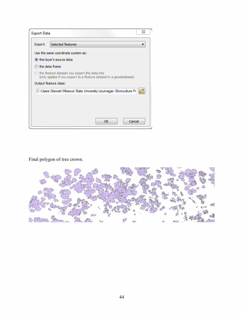
44

Final polygon of tree crown.