
Modeling, Simulation and Design of Dye Sensitized Solar Cells
39
Modeling, Simulation and Design of Dye Sensitized Solar Cells José Maçaira, Luísa Andrade*, Adélio Mendes* LEPAE - Departamento de Engenharia Química, Universidade do Porto - Faculdade de Engenharia, Rua Dr. Roberto Frias, s/n 4200-465 Porto, Portugal l[email protected], [email protected] Abstract It is well known that recombination and transport rule the performance of dye sensitized solar cells (DSC’s); although, the influence that these two phenomena have in their performance, particularly in the open circuit-potential (V oc ) and in the short circuit current (J sc ), is not fully understood. In this paper a phenomenological model is used to describe the quantitatively effect that transport and recombination have in the performance of the solar cell and their influence in its optimal design. The model is used to predict the influence of the recombination reaction rate constant (k r ) and diffusion coefficient (D eff ) in the V oc and in the J sc , whether a linear or non-linear recombination kinetic is considered. It is provided a methodology for decoupling the conduction band shifts from recombination effect in charge extraction experiments. Results also suggest that the influence of recombination in the V oc and in J sc is highly dependent on the reaction order considered. This fact highlights the importance of considering the reaction order when modeling data obtained by experimental methods. The combined results are analyzed and discussed in terms of the collection efficiency and in the optimization of the photoelectrode thickness. The model provides also a useful framework for exploring new concepts and designs for improving DSCs performance. Introduction The dye sensitized solar cell (DSC) is a potentially low cost photovoltaic technology that recently has achieved 12 % efficiency by two different approaches 1, 2 . A very recent work reported an energy conversion efficiency of 15 % for a new sensitized solar cell 3 . This world
Transcript of Modeling, Simulation and Design of Dye Sensitized Solar Cells

Modeling, Simulation and Design of Dye Sensitized Solar Cells
José Maçaira, Luísa Andrade*, Adélio Mendes*
LEPAE - Departamento de Engenharia Química, Universidade do Porto - Faculdade de
Engenharia, Rua Dr. Roberto Frias, s/n 4200-465 Porto, Portugal
[email protected], [email protected]
Abstract
It is well known that recombination and transport rule the performance of dye sensitized
solar cells (DSC’s); although, the influence that these two phenomena have in their
performance, particularly in the open circuit-potential (Voc) and in the short circuit current (Jsc),
is not fully understood. In this paper a phenomenological model is used to describe the
quantitatively effect that transport and recombination have in the performance of the solar cell
and their influence in its optimal design. The model is used to predict the influence of the
recombination reaction rate constant (kr) and diffusion coefficient (Deff) in the Voc and in the Jsc,
whether a linear or non-linear recombination kinetic is considered. It is provided a methodology
for decoupling the conduction band shifts from recombination effect in charge extraction
experiments. Results also suggest that the influence of recombination in the Voc and in Jsc is
highly dependent on the reaction order considered. This fact highlights the importance of
considering the reaction order when modeling data obtained by experimental methods. The
combined results are analyzed and discussed in terms of the collection efficiency and in the
optimization of the photoelectrode thickness. The model provides also a useful framework for
exploring new concepts and designs for improving DSCs performance.
Introduction
The dye sensitized solar cell (DSC) is a potentially low cost photovoltaic technology
that recently has achieved 12 % efficiency by two different approaches1, 2
. A very recent work
reported an energy conversion efficiency of 15 % for a new sensitized solar cell 3. This world

Modeling, Simulation and Design of Dye Sensitized Solar Cells
‒ 2 ‒
record has been announced by M. Gräztel at the Hybrid and Organic Photovoltaic conference
(HOPV 2013) meeting held in Seville in 2013 and has been certified as 14 % of energy
efficiency by Newport Corporation3. Dye sensitized solar cells (DSCs) mimic natural
photosynthesis and differ from conventional p-n junction devices because light collection and
charge transport are separated in the cell 4. Light absorption occurs in the chemisorbed sensitizer
molecule, while electron transport occurs in the semiconductor. The photo conversion energy
efficiency (η) of the solar cell is determined by its current-potential characteristics, specifically
the open-circuit photopotential (Voc), the photocurrent density measured under short-circuit
conditions (Jsc), the intensity of incident light (Is) and the fill factor of the cell (FF). The
working principles of DSCs, illustrated in Figure 1, can be summarized in the following steps:
a. Light harvesting: photon absorption by dye molecules adsorbed in a monolayer on the
surface of the mesoporous semiconductor (typically TiO2); electrons from the ground
state (S) are promoted to the excited state (S*, k11):
S
ℎ𝑣 ,𝑘11 → 𝑘12
← S∗ (1)
b. Injection: the excited electrons are injected into the conduction band of the
semiconductor (k21), resulting in the oxidation of the sensitizer (S+):
S∗
𝑘21 → 𝑘22
← S
+ + e𝐶𝐵−
(2)
c. Dye regeneration: reduction of the oxidized sensitizer (S+) to its original state (S) by
electron donation from I- present in the liquid electrolyte, producing I3
− (k3):
S+ +3
2I−
𝑘3 →
1
2I3− + S (3)
d. Collection: diffusive collection of electrons from the mesoporous semiconductor to the
transparent conductive oxide (TCO) where they become available for electrical work
in the external circuit;

José Maçaira, Luísa Andrade, Adélio Mendes
‒ 3 ‒
e. Electrolyte mass transfer: diffusive transport of the reduced I3− and oxidized I
- through
the pores of the semiconductor to and from the counter electrode (usually coated with
a platinum catalyst);
f. Electrolyte regeneration: at the counter electrode the platinum catalyst reduces the
oxidized I3−
back to I- by reaction with a low energy electron from the external circuit
(k4):
I3− + 2e−
𝑃𝑡 ,𝑘4 → 3I− (4)
During this series of reactions, there are also processes that are unfavorable to the DSC
performance:
g. Decay of dye excited state: decay of the excited state of the dye (S+) to the ground
state (S) before electron injection in the conduction band of the semiconductor. This
reaction (k12) competes directly with the injection step (k21);
h. Electron-dye recombination (k22): reaction between the oxidized dye molecules (S+)
with electrons in the conduction band of the TiO2. This competes with dye
regeneration (k3) and with collection of electrons from the TiO2 (d);
i. Electron-electrolyte recombination: reaction of conduction band electrons with
electrolyte species. This reaction competes with electron collection (d).
I3− + 2e𝐶𝐵
− 𝑘5 → 3I− (5)

Modeling, Simulation and Design of Dye Sensitized Solar Cells
‒ 4 ‒
Fig. 1 Illustration of DSC’s working principles. The full arrows represent the forward electron transfer
reactions; the dashed arrows represent electron losses routes.
For solar cell to produce electrical energy, the forward electron transfer reactions (k11,
k21, k3 and k4) must overcome the possible electron lost pathways (k12, k22 and k5). The time
constant ranges of each reaction are illustrated in Figure 2 5. The recombination reaction of
electrons with electrolyte species (k5) is considered to be one of the most important energy
efficiency bottlenecks. Because the electrolyte is present throughout all the porous structure of
the semiconductor, the recombination reaction is affected by the photoelectrode thickness,
iodide concentration, dye structure and others. 6-9
The average electron diffusion coefficients in anatase TiO2 ranges between 10-4
to 10-5
cm2∙s
-1 10, resulting in an electron transport time constant (τtr) for a typical 10 µm thick
photoelectrode in the range of few milliseconds. The electron lifetime (τe-) corresponding to a
recombination reaction constant of k5 – Figure 2, has the same order of magnitude of the
electron transport time constant resulting in a directly competition between these two
mechanisms. The current and potential outputs of the DSC are recombination limited, and result

José Maçaira, Luísa Andrade, Adélio Mendes
‒ 5 ‒
from a balance between the charge generation and the recombination fluxes. Controlling charge
extraction, by increasing transport, and lowering charge recombination will increase the
efficiency of DSCs. Thus, understanding charge recombination and controlling recombination
rate constants is of utmost importance. Several studies have been carried out to understand how
recombination can been lowered in DSCs, and many articles have been published examining the
effect of electrolyte additives, new photoanode architectures, new dyes, surface coatings, among
other factors 11-23
.
Fig. 2 Time constant ranges of the reactions in a DSC.
In this work a dynamic phenomenological model proposed initially by Andrade et al. 24
is used to describe the quantitatively effect that transport and recombination have in the
performance of the solar cell, and the influence that this has in its design. The model is used to
predict the influence of the recombination reaction rate constants (kr) and diffusion coefficients
(Deff) in the Voc and Jsc, considering linear or non-linear recombination reaction. The results are
helpful, particularly in decoupling phenomena seen in charge extraction experiments that are
usually used to assess and compare recombination rates among DSC samples.
Modeling
The model used in this work is based on the initially proposed model by Andrade et al
24 but taking into account the recombination reaction order parameter β. The mobile species
considered in the present model are electrons in the conduction band of TiO2 and iodide and

Modeling, Simulation and Design of Dye Sensitized Solar Cells
‒ 6 ‒
triiodide ions in the liquid electrolyte. The developed model of an irradiated DSC assumes the
following physical and chemical processes:
1) electron generation (from excited dye molecules);
2) electron transport in the porous semiconductor (TiO2);
3) electron recombination with electrolyte species;
4) oxidation of iodide (inside the pores of TiO2);
5) and reduction of triiodide (at the platinum catalyst).
It is assumed that the cell is irradiated perpendicularly to the photoelectrode and that
each absorbed photon generates one injected electron into the TiO2 conduction band. All
injected electrons are considered from the excited state of the dye, and not from TiO2 band gap
excitation. Reactions (1) and (2) are considered irreversible since their forward kinetic constants
are much higher that the corresponding reverse kinetic constants (k11 >> k12 and k21 >> k22) 5.
Therefore only one possible mechanism for electron loss is assumed, corresponding to the
recombination reaction of electrons with electrolyte species (5).
Figure 3 illustrates the modeled DSC. The photoelectrode is deposited over the TCO
layer, which has an electrical resistance of RTCO, and is made of a film of sintered TiO2
nanoparticles with thickness Lf and porosity ε. The dye is adsorbed on this mesoporous film of
TiO2 as a monolayer. The dye has a wavelength-dependent light absorption coefficient of α(λ).
The liquid electrolyte, made of the redox pair I−/ I3− (with diffusion coefficients 𝐷I−and 𝐷I3−), is
responsible for the regeneration of the dye, transporting low energy electrons from the counter-
electrode. The TCO-TiO2 interface was defined to be at x = 0. This interface is modeled as an
ideal ohmic contact, meaning that there is no charge transfer resistance at the interface. At the
counter electrode, the interface electrolyte-platinum catalyst happens at x = L and the
electrochemical reduction of I3− was described by the Butler-Volmer equation. The electron
transport in the photoelectrode was assumed to be governed by diffusion (negligible convection)
18.

José Maçaira, Luísa Andrade, Adélio Mendes
‒ 7 ‒
Fig. 3 Scheme of the modeled DSC.
From the previous assumptions, the continuity and transport equation that describe the
mobile species is24
:
−𝜕𝐽𝑖
𝜕𝑥+ 𝐺𝑖(𝑥) − 𝑅𝑖(𝑥) =
𝜕𝑛𝑖
𝜕𝑡, 𝑖 = e− , I3
− , I− (6)
The first term on the left hand side of equation (6) represents the charge carrier flux. The second
and third terms, Gi(x) and Ri(x), represent the generation and recombination rates of species i,
respectively. The term on the right hand side of the equation is the concentration species i time
derivative. The charge carrier flux, Ji, is assumed to occur by diffusion only and is given by the
Fick’s law25
:
𝐽𝑖 = −𝐷𝑖𝜕𝑛𝑖
𝜕𝑥 (7)
and the generation rate is given by the Beer-Lambert law that relates the absorption of light to
the properties of the material through which the light is travelling:
𝐺𝑖 = 𝜂inj𝛼(𝜆)𝐼0𝑒−𝛼(𝜆)𝑥 (8)
Each absorbed photon is assumed to produce one injected electron. The developed model
considers a uniformly distributed monolayer of dye through the surface area of TiO2. The
injection efficiency parameter, 𝜂inj, takes into account this phenomenon but also the light
reflection and glass and electrolyte absorption losses.

Modeling, Simulation and Design of Dye Sensitized Solar Cells
‒ 8 ‒
For each two electrons that react with triiodide, three ions of iodide are formed (reaction
5). The recombination rate term can be written as follows26
:
𝑅e− = 𝑘𝑟(𝑛e−(𝑥, 𝑡) − 𝑛eq)𝛽
(9)
The recombination reaction kinetics is subject of much debate and some of the scientific work
published so far considers that this reaction follows first-order kinetics:
𝛽 = 1 ; 𝑘𝑟 =1
𝜏e− (10)
where kr is the reacton rate constant and 𝜏e− is the electron lifetime.
However, several uncertainties surround the recombination kinetics in DSCs and the
respective parameters that govern the solar cells behavior. Some models assume that the rate at
which electrons are transferred from the conduction band to the redox electrolyte is first order in
free electron concentration (β = 1) 27, 28
. However, it has been suggested that deviations from the
first order model may arise from the recombination process being mediated by electronic
surface states below the TiO2 conduction band 29-31
. A non-linear model formulation has then
being suggested:
𝛽 ≠ 1 ; 𝑘𝑟 = 𝑘01
𝜏e− (11)
where kr is the reaction rate constant and k0 is a model constant. The driving force of the
recombination reaction is the diference between the generated electrons density, 𝑛e−(𝑥, 𝑡), and
the dark equilibrium electron density, 𝑛eq. This electron density corresponds to the resulting
equilibrium bewteen the electron at the fermi level and the redox potential of the electrolyte:
𝑛eq = 𝑁CB exp [−𝐸CB −𝐸redox
kB𝑇] (12)
According to the above assumptions the model equations can be written as follows:
Electrons balance
Introducing equations (7), (8), and (9) into the continuity equation (6), the continuity
equation for electrons comes:
𝐷e−𝜕2𝑛e−
𝜕𝑥2+ 𝜂inj𝛼(𝜆)𝐼0𝑒
−𝛼(𝜆)𝑥 − 𝑘𝑟(𝑛e−(𝑥, 𝑡) − 𝑛eq)𝛽=
𝜕𝑛e−
𝜕𝑡 (13)

José Maçaira, Luísa Andrade, Adélio Mendes
‒ 9 ‒
Assuming that for t = 0 the cell is not illuminated, the electron density is equal to the dark
electron density, neq:
𝑡 = 0 𝑛e− (𝑥, 0) = 𝑛eq (14)
A charge balance at the interface x = 0 determines that the electron flux at x=0+ equals
the electron flux at x=0-. Therefore, the charge balance at this interface is given by 𝐽e−
0+ = 𝐽e−0−.
Because 𝐽e−0+ corresponds to the diffusive electrons transported through the TiO2, which in
steady state is the net current produced by the solar cell, Jcell, the boundary condition for x=0 is:
𝑥 = 0 ; 𝐽e−0+ = − q𝐷e−
∂ne−
∂x𝑥=0+ (16)
At x=L there is no contact between the film of TiO2 nanoparticles and the platinized
FTO. Therefore, there are no electrons bridging between the photoelectrode and the couter-
electrode. Only iodide and triiodide perform this charge transfer. Thus, the corresponding
boundary condition for x = L is:
𝑥 = 𝐿 ;𝜕𝑛e−
𝜕𝑥 = 0 (17)
Iodide and Triiodide balance
Each generated mole of electrons causes the consumption of one mole of I- ion and the
production of half mole of I3- that can be reduced back to I
- form either at the platinum layer or
due to the recombination reaction (undesirable back reaction). Besides the reduction of triiodide
that takes place at the counter-electrode, the oxidation and reduction reactions of the ionic
species take place in the photoelectrode porosity. Accordingly to the stoichiometry reactions (3)
and (4) the terms of generation and recombination of triiodide and iodide must be affected by
the corresponding coefficients:
𝐷I−𝜕2𝑛I−
𝜕𝑥2−
3
2𝜀𝑝[𝜂inj𝛼(𝜆)𝐼0𝑒
−𝛼(𝜆)𝑥 − 𝑘𝑟(𝑛e−(𝑥, 𝑡) − 𝑛eq)𝛽−
𝜕𝑛e−(𝑥,𝑡)
𝜕𝑡 ] =
𝜕𝑛I−(𝑥,𝑡)
𝜕𝑡 (18)
𝐷I3−𝜕2𝑛I3
−
𝜕𝑥2+
1
2𝜀𝑝[𝜂inj𝛼(𝜆)𝐼0𝑒
−𝛼(𝜆)𝑥 − 𝑘𝑟(𝑛e−(𝑥, 𝑡) − 𝑛eq)𝛽−
𝜕𝑛e−(𝑥,𝑡)
𝜕𝑡 ] =
𝜕𝑛I3−(𝑥,𝑡)
𝜕𝑡 (19)
At instant t=0, the concentration of iodide and triiodide is known:
Modeling, Simulation and Design of Dye Sensitized Solar Cells
‒ 10 ‒
𝑡 = 0 ∶ 𝑛I3−(𝑥, 0) = 𝑛I3−ini ; 𝑛I−(𝑥, 0) = 𝑛I−
ini (21)
At the interface of TiO2/TCO, x = 0, only electrons are able to flow so the net flux of
I3− and I− is zero:
𝑥 = 0 ∶ 𝜕𝑛I3
−
𝜕𝑥 = 0 ;
𝜕𝑛I−
𝜕𝑥 = 0 (22)
Although there is generation and consumption of both ionic species, their total number
of moles remains constant, thus resulting in the following integral boundary condition:
𝑥 = 𝐿 : ∫ 𝑛I3−(𝑥)𝑑𝑥𝐿
0= 𝑛I3−
ini 𝐿 ; ∫ 𝑛I−(𝑥)𝑑𝑥𝐿
0= 𝑛I−
ini 𝐿 (23)
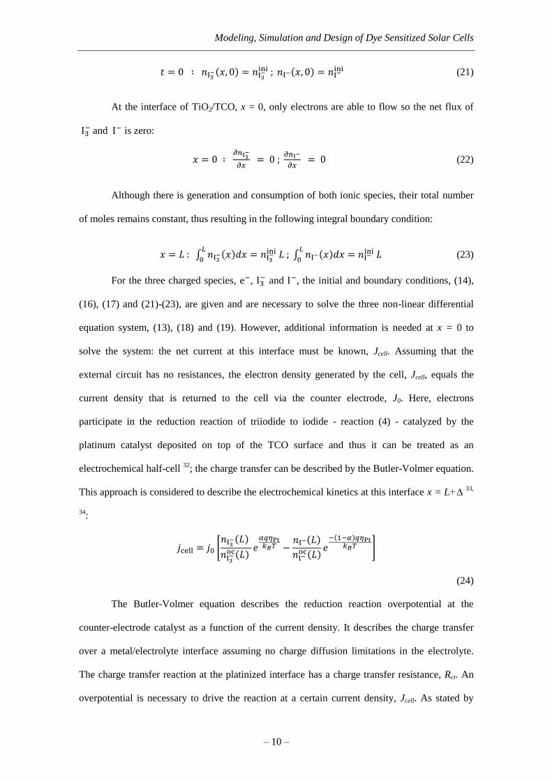
For the three charged species, e−, I3− and I−, the initial and boundary conditions, (14),
(16), (17) and (21)-(23), are given and are necessary to solve the three non-linear differential
equation system, (13), (18) and (19). However, additional information is needed at x = 0 to
solve the system: the net current at this interface must be known, Jcell. Assuming that the
external circuit has no resistances, the electron density generated by the cell, Jcell, equals the
current density that is returned to the cell via the counter electrode, J0. Here, electrons
participate in the reduction reaction of triiodide to iodide - reaction (4) - catalyzed by the
platinum catalyst deposited on top of the TCO surface and thus it can be treated as an
electrochemical half-cell 32
; the charge transfer can be described by the Butler-Volmer equation.
This approach is considered to describe the electrochemical kinetics at this interface x = L+∆ 33,
34:
𝑗cell = 𝑗0 [𝑛I3−(𝐿)
𝑛I3−oc(𝐿)
𝑒𝛼𝑞𝜂Pt𝑘𝐵𝑇 −
𝑛I−(𝐿)
𝑛I−oc(𝐿)
𝑒−(1−𝛼)𝑞𝜂Pt
𝑘𝐵𝑇 ]
(24)
The Butler-Volmer equation describes the reduction reaction overpotential at the
counter-electrode catalyst as a function of the current density. It describes the charge transfer
over a metal/electrolyte interface assuming no charge diffusion limitations in the electrolyte.
The charge transfer reaction at the platinized interface has a charge transfer resistance, Rct. An
overpotential is necessary to drive the reaction at a certain current density, Jcell. As stated by

José Maçaira, Luísa Andrade, Adélio Mendes
‒ 11 ‒
equation (24), the current density of the cell depends on the exchange current density, J0, which
is the electron’s ability to exchange with the solution, but also with the platinum overpotential,
ηPt. This value translates the necessary potential to overcome the energy barrier of the reaction
of the electrons with the triiodide. This corresponds to an overall potential loss of the solar cell
and must be as low as possible 35, 36
. The counter electrode overpotential, ηPt, can be obtained as
follows: 24
Δ𝑉int =1
𝑞[𝐸CB + 𝑘𝐵𝑇 ln
𝑛e−(𝑥=0)
𝑁CB− 𝐸redox
0 −𝑘𝐵𝑇
2ln
𝑛I3−oc
(𝑛I−oc𝐿)3
− 𝑞𝜂Pt] ⟺
𝜂Pt =𝐸CB−𝐸redox
oc
𝑞+
𝑘𝐵𝑇
𝑞[ln
𝑛I3−oc
2(𝑛I−oc𝐿)
3 + ln𝑛e−(𝑥=0)
𝑁CB] − Δ𝑉int (33)
Analyzing equation (33) is understood that ηPt, and consequently the electrons flux,
depends on the internal potential of the solar cell. There are also external resistances that should
be accounted for and correlated to the internal resistances; this can be done using Kirchhoff’s
and Ohm’s laws 32
:
∆𝑉int = (𝑅series + 𝑅ext) (𝑅𝑝
𝑅ext+𝑅series+𝑅𝑝)𝐴 𝐽cell (34)
where Rseries is the sum of all external resistances, Rext is the applied load, Rp are the shunt
resistances, and A the active area of the DSC. Equation (34) should be inserted in counter
electrode overpotential equation (33) and then introduced in the Butler-Volmer equation (24).
Thus the produced current of the solar cell, equation (24), can be determined by the applied
load, Rext. The external potential given by the device is calculated taking into account the
produced current, the applied load and the other resistances taken into account in the model:
𝑉ext = 𝑅ext (𝑅𝑝
𝑅ext+𝑅series+𝑅𝑝)𝐴 𝐽cell (35)
To decrease the number of variables and to improve numerical convergence issues of
the numerical methods, the model parameters were made dimensionless respecting to the
electron and ionic species parameters and the semiconductor thickness:

Modeling, Simulation and Design of Dye Sensitized Solar Cells
‒ 12 ‒
𝛾 = 𝛼(𝜆)𝐿, 𝜃 =𝐷ref
𝐿2𝑡, 𝑛𝑖
∗ =𝑛𝑖
𝑛ref, 𝑥∗ =
𝑥
𝐿,
𝐷𝑖∗ =
𝐷𝑖
𝐷ref, 𝑗cell
∗ =𝑗cell
𝑗0, 𝐷𝑎 =
𝐿2𝜂inj𝛼(𝜆)𝐼0
𝐷ref𝑛ref, 𝜙 = 𝐿√
𝑘𝑟
𝐷ref
Using the above established dimensionless variables, the dimensionless equations and
respective initial and boundary conditions can be written as follows for the three modeled
species (e− , I3− and I−):
Dimensionless Electrons Balance
𝐷e−∗ 𝜕𝑛e−
∗
𝜕𝑥∗2+ [𝐷𝑎 𝑒−𝛾𝑥
∗− 𝜙2(𝑛e−
∗ − 𝑛eq∗ )
𝛽] =
𝜕𝑛e−∗
𝜕𝜃 (36)
Initial condition:
𝜃 = 0 ; 𝑛e−∗
(𝑥∗, 0) = 𝑛eq
∗ (37)
Boundary conditions:
𝑥∗ = 0 ; 𝐽cell∗ =
𝑛ref𝐷ref 𝑞
𝐿(𝐷e−
𝜕𝑛e−∗
𝜕𝑥∗𝑥=0+ ) ; 𝑥∗ = 1;
𝜕𝑛e−∗
𝜕𝑥∗= 0 (38)
Dimensionless Triiodide Balance
𝐷I3−∗𝜕2𝑛I3
−∗
𝜕𝑥∗2+
1
2𝜀𝑝[𝐷𝑎 𝑒−𝛾𝑥
∗− 𝜙2(𝑛e−
∗ − 𝑛eq∗ )
𝛽−
𝜕𝑛e−∗
𝜕𝜃] =
𝜕𝑛I3−∗
𝜕𝜃 (39)
Initial condition:
𝜃 = 0 ; 𝑛I3−∗ (𝑥∗, 0) = 𝑛I3−
∗ 𝑖𝑛𝑖 (40)
Boundary conditions:
𝑥∗ = 0 ;𝜕𝑛I3
−∗ (0,𝜃)
𝜕𝑥∗= 0 ; 𝑥∗ = 1 ; ∫ 𝑛I3−
∗ (𝑥∗)𝑑𝑥∗1
0= 𝑛I3−
∗𝑖𝑛𝑖 (41)
Dimensionless Iodide Balance

José Maçaira, Luísa Andrade, Adélio Mendes
‒ 13 ‒
DI−∗ ∂2nI−
∗
∂x∗2−
3
2εp[Da . e−γx
∗− ϕ2(ne−
∗ − neq∗ )
β−
∂ne−∗
∂θ] =
∂nI−∗
∂θ (42)
Initial condition:
𝜃 = 0 ; 𝑛I−∗ (𝑥∗, 0) = 𝑛I−
∗ ini (43)
Boundary conditions:
𝑥∗ = 0 ;𝜕𝑛𝐈−
∗ (0,𝜃)
𝜕𝑥∗= 0 ; 𝑥∗ = 1 ; ∫ 𝑛I−
∗ (𝑥∗)𝑑𝑥∗1
0= 𝑛I−
∗ini (44)
The system of equations (36), (39) and (42) describes the history of the mobile species
concentration profiles. The partial differential equations were spatially discretized using the
finite differences method. The time integration was accomplished by the numerical package
developed by the Lawrence Livermore National Laboratory, LSODA 37
.
Experimental
Dye sensitized solar cell preparation
Steady state simulated results were critically compared with experimental results of two
DSCs with different photoelectrode thicknesses: device A with 7.5 µm and device B with
12.5µm. The photoelectrodes were prepared on 2.2 mm thick and 7 Ω/ FTO coated glass
substrates from Solaronix®. First, the glasses were washed sequentially with a detergent
solution (Alconox® , VWR) in an ultrasonic bath at 55 ºC for 15 min, followed by ultrasonic
cleaning in deionized water at room temperature, rinsed with ethanol and dried with air. To
form a thin and compact layer of TiO2 above the FTO layer, the substrates were immersed in a
40 mM TiCl4 aqueous solution at 70ºC, for 20 minutes. After washing with water and ethanol,
the samples were dried with a nitrogen flow. Then, the samples were coated with porous TiO2
layer by screen printing a commercial TiO2 paste (Ti-Nanoxide T/SP from Solaronix®),
followed by drying at 80 ºC for 20 minutes. To control the final thickness of the transparent
layer of TiO2, the screen printing procedure (printing and drying) was repeated as necessary to

Modeling, Simulation and Design of Dye Sensitized Solar Cells
‒ 14 ‒
get the desired thickness of photoelectrode. The samples were annealed at 500 ºC for 15 min in
an infrared electrical oven. After firing, the samples were again treated with a 40 mM TiCl4
aqueous solution at 70 ºC for 20 minutes, before being sintered at 500 ºC for 30 min. The
counter electrodes, prepared on the same type of glass substrates and cleaned as described
before, were drilled previously with two holes of 1 mm diameter. A drop of H2PtCl6 solution (2
mg of Pt in 1 mL ethanol) was applied on the glass substrate followed by annealing at 400 ºC
for 15 minutes. Both electrodes were assembled and sealed using a laser assisted glass frit
method described elsewhere 38
. Dye adsorption in the porous TiO2 was obtained recirculating 1
mM N719 dye solution for 10 hours, followed by ethanol rinsing, nitrogen drying, electrolyte
filling (Iodolyte Z-150 from Solaronix®) and hole sealing by thermoplastic sealant (Surlyn®,
Dupont).
Results and Discussion
Current-Potential Characteristics
The input values of parameters for the simulation step are listed in Table 1. For each
parameter it is indicated if the value was obtained by fitting to the experimental results
(parameters kr, β and Ec-Eredox) or from an independent source.
The experimental I-V characteristics were obtained in a set-up equipped with a 1600 W
xenon light source (Oriel class B solar simulator, Newport, USA) irradiating 100 mW·cm-2
(1
sun light intensity) and using a 1.5 air mass filter (Newport, USA). The simulator was calibrated
using a single crystal Si photodiode (Newport, USA). The I-V characteristics of the solar cell
were obtained applying an external potential bias (electrical load) and measuring the generated
photocurrent.

José Maçaira, Luísa Andrade, Adélio Mendes
‒ 15 ‒
Table 1. Input values for the simulation step for device A and B.
Parameter notation Device A Device B Ref
Morphological
features
Cell Thickness L / μm 7.5 12.5 Measured
Film Porosity ε 0.63 Computed
Active area A / cm2 0.158 Measured
Photon
absorption/
electron
Injection
Incident Photon Flux Is / cm-2·
s-1
1.47×10¹⁷
Measured
Injection Efficiency ηinj 0.90 39
Dye Absorption
Coefficient α(λ) / cm
-1 1000 Computed
Temperature T / K 298 Measured
Initial/boundary
concentrations
of species
Initial
Concentrations
C0
e- 0 -
𝐶𝐼3−0 /mmol·dm
-3 100.0 Computed
𝐶𝐼−0 / mmol·dm
-3 1100 Computed
Open-Circuit
Concentrations
𝐶𝐼3−oc
/ mmol·dm-3
99.00 Computed
𝐶𝐼−oc / mmol·dm
-3 1102 Computed
Diffusion
coefficients of
species
Diffusion
coefficients
𝐷𝐼3− / cm2·s
-1 4.91×10
-6
24
𝐷𝐼− / cm2·s
-1 4.91×10
-6
24
Deff / cm2·s
-1 1.10 × 10
-4
24
Pt Counter
electrode
Exchange Current
Density j0 / mA·cm
-2 6.81 × 10
-2 Computed
Symmetry
Parameter α 0.78
32
Recombination
reaction
Reaction order
coefficient β 0.75 Fit
Rate constant kr / m-0.75
·s-1
8.00 6.62 Fit
Density of
States
Ecb - Eredox eV 0.93 0.94 Fit
Effective density of
states in the TiO2
conduction band
Nc / cm-3
1.00 × 10²¹
40
External
Resistances
Shunt Resistances Rp / Ω 76129 14392 Computed
External Series
resistances Rseries / Ω 40 47 Computed
Figure 4 plots the experimental and simulated I-V and power curves for the two sets of
samples. The experimental and simulated results are in good agreement. Table 2 present the
experimental and simulated performance parameters; the relative different between both is
smaller than 2 % giving showing that the model is able to simulate accurately the experimental
results.

Modeling, Simulation and Design of Dye Sensitized Solar Cells
‒ 16 ‒
Fig. 4 Experimental and simulated results I-V and power curves for device A and B (photoelectrode with
7.5 µm and 12.5 µm thickness). All other parameters are presented in Table 1.
Table 2. Performance parameters of the simulated and experimental results.
Semiconductor
thickness 12.5 µm 7.5 µm
Performance
Parameter Simulation Experimental (Error %) Simulation Experimental (Error %)
Jsc / mA·cm-2
12.93 12.95 (0.1) 10.21 10.23 (0.2)
Voc / V 0.75 0.76 (0.6) 0.76 0.76 (0.7)
Max. PP
/mW·cm-2
7.18 7.12 (0.9) 5.98 5.88 (1.7)
Vmpp / V 0.61 0.60 (1.2) 0.62 0.62 (0.0)
Jmpp / mA·cm-2
11.85 11.89 (0.1) 9.63 9.48 (1.6)
Fill Factor 0.74 0.73 (1.4) 0.77 0.76 (1.2)
Efficiency, η 7.18 7.12 (0.9) 5.98 5.88 (1.7)
0
2
4
6
8
10
12
14
16
0
2
4
6
8
10
12
14
16
0.00 0.10 0.20 0.30 0.40 0.50 0.60 0.70 0.80
Po
wer
/ m
W.c
m-2
Cu
rren
t D
ensi
ty/
mA
. cm
-2
Potential /V
Experimental I-V, device B Experimental I-V, device A
Experimental power curve, device B Experimental power curve, device A
Model

José Maçaira, Luísa Andrade, Adélio Mendes
‒ 17 ‒
Even though the model predicts the experimental results reasonably well, there are some
deviations, particularly in the maximum power point. The deviation is caused by the difference
in the simulated and experimental fill factor. This difference probably relates to the rough
estimation made for the shunt resistance. The shunt resistance relates to the back electron
transfer across the TiO2/dye/electrolyte interface, particularly in the dye free areas of the TiO2
surface and can be estimated from the slope of the experimental I-V curve at short circuit.41
Influence of recombination in DSCs
Controlling the recombination reaction is believed to be the key to developing new
materials and cell architectures for high efficient DSCs. Thus the interpretation of the
recombination rate constants influence in the working mechanisms of DSCs is of extreme
importance. 40, 42
. In the previous section the model was compared to experimental results and
proved to model well the steady state behavior of the prepared DSCs. In this section, the
influence of kr in the performance of the solar cell is assessed. This parameter affects the
amount of generated electrons that react back to the electrolyte. Figure 5 shows the simulated I-
V curves for recombination rate constants ranging from 5 to 1000 s-1
(β = 1). Clearly, the I-V
curve is affected by the amount of electrons that recombine, which is reflected particularly in
the Jsc and Voc values.

Modeling, Simulation and Design of Dye Sensitized Solar Cells
‒ 18 ‒
Fig. 5 Simulated I-V curves with different recombination reaction rate constants. All other parameters are
presented in Table 1, device B.
Figure 6 shows the simulated electron density profiles at steady-state conditions and the
theoretical photon absorption/electron generation through the TiO2 film according to the Beer-
Lambert law. Since solar radiation is assumed to strike the photoanode side of the solar cell (see
Figure 3), at x = 0, most of the electrons are generated near this interface, due to the exponential
behavior of the absorption law. For this reason, and also because the transport path for the
generated electrons increases from x = 0 to 12.5 µm, a larger electron density gradient is seen at
the beginning of the film decreasing towards zero at positions close to x = 12.5 µm. This
indicates that the initial TiO2 layer thickness fraction closer to the illuminated side of the solar
cell is the one that contribute the most for the current delivered by the cell. The change in the
electron lifetime (assumed first order recombination) has a strong influence in the electron
density across the semiconductor. The electron density profiles have been simulated for short-
circuit (Figure 6), maximum power point (Figure 7) and open circuit conditions (Figure 8). As
expected, for higher recombination rates the concentration of electrons are lower justifying the
lower values of Jsc (Figure 6) and Voc (Figure 8) parameters.
0
2
4
6
8
10
12
14
16
0.00 0.20 0.40 0.60 0.80 1.00
Cu
rren
t D
ensi
ty /
mA
·cm
-2
Potential /V
Recombination r
rate constant kr / s-1
5
10
22
43
85
170

José Maçaira, Luísa Andrade, Adélio Mendes
‒ 19 ‒
Fig. 6 Simulated electron density profiles for short circuit conditions with different recombination
reaction rate constants. All other parameters are presented in Table 1, device B.
Fig. 7 Simulated electron density profiles for maximum power point with different recombination
reaction rate constants. All other parameters are presented in Table 1, device B.
0
2
4
6
8
10
12
14
0
5
10
15
20
25
30
35
40
45
0 2 4 6 8 10 12
Ele
ctro
n g
ener
ati
on
/ x
10
19 c
m-3
Ele
ctro
n d
ensi
ty /
x 1
016 c
m-3
Position x in TiO2 / μm kr / s
-1 20 45 65 200 Electron generation
0
2
4
6
8
10
12
14
0
10
20
30
40
50
60
0 2.5 5 7.5 10 12.5
Ele
ctro
n g
ener
ati
on
/ x
10
19 c
m-3
Ele
ctro
n d
ensi
ty /
x1
016 c
m-3
Position x in TiO2 / μm
kr / s-1
20 45 65 200 1000 Electron generation

Modeling, Simulation and Design of Dye Sensitized Solar Cells
‒ 20 ‒
Fig. 8 Simulated electron density profiles for open circuit conditions with different recombination
reaction rate constants. All other parameters are presented in Table 1, device B.
At open circuit conditions the recombination flux matches the photocurrent and there
are no electrons flowing to the external circuit. At these conditions there is almost no electron
gradient, as seen in Figure 8, and this equilibrium determines the open circuit potential, Voc, of
the device.26
Therefore, recombination determines the open potential, Voc, of the device and also
controls the short circuit current, Jsc. The excited electron density profiles in the TiO2 film,
simulated for different electron recombination rates, enlighten the influence that this reaction
has in the open potential, Voc, of the solar cell. The electron recombination rate affects the
electron flow through the external circuit, and therefore, affects the chemical potential that is
built inside the device due to the presence of energy states below the Fermi level of the
semiconductor. This way, the amount of electrons that react with the triiodide affects the final
potential of the system, as can be confirmed in Figure 8 where higher recombination rates
reduce the electron density in the device at open circuit conditions and, by doing so, the
chemical potential within the device, acts to reduce the final Voc of the solar cell.
The concentration profiles of the ionic species, shown in Figure 9, are also influenced
by recombination. For an illuminated cell, triiodide is formed where there is photon absorption
0
2
4
6
8
10
12
14
0
50
100
150
200
250
300
350
400
0 2.5 5 7.5 10 12.5
Ele
ctro
n g
ener
ati
on
/ x
10
19 c
m-3
Ele
ctro
n d
ensi
ty /
x1
016 c
m-3
Position x in TiO2 / μm kr / s
-1
20 45 65 200 1000 Electron generation
Recombination
increase

José Maçaira, Luísa Andrade, Adélio Mendes
‒ 21 ‒
and consequently electron injection, due to the regeneration reaction of the oxidized dye with
iodide, producing triiodide. Therefore electron generation increases the consumption of iodide
and consequently the formation of triiodide. By increasing the recombination reaction rate
constant, the amount of electrons that react with triiodide is higher, and thus there is an extra
consumption of triiodide besides the amount that is produced by the regeneration reaction of
iodide with the oxidized dye. However, because there are less electrons flowing to the external
circuit and being returned back to the device through the counter electrode, there is an
accumulation of triiodide, mainly at the interface x = 12.5 µm, where the reduction reaction
back to iodide takes place at the platinum catalyst. Along with the extra consumption of
triiodide higher kr also causes higher formation of iodide; because the fraction of iodide
consumption due to the dye regeneration is independent of kr, for higher recombination rates
there an accumulation of I- s verified for x=0 - Figure 9.
Fig. 9 Simulated ionic concentration profiles for maximum power point for different recombination
reaction rate constants. All other parameters are given in Table 1, device B.
0.82
0.84
0.86
0.88
0.90
0.92
0.94
0.96
0.98
1.00
0.950
0.955
0.960
0.965
0.970
0.975
0.980
0.985
0.990
0.995
1.000
0 2 4 6 8 10 12
Ad
imen
sio
na
l T
riio
did
e co
nce
ntr
ati
on
Ad
imen
sio
na
l Io
did
e co
nce
ntr
ati
on
Position x in TiO2 / μm specie, kr /s
-1
Iodide, 20 Iodide , 45 Iodide, 200
Iodide , 1000 Triiodide, 20 Triiodide, 45

Modeling, Simulation and Design of Dye Sensitized Solar Cells
‒ 22 ‒
The effect of recombination in the open circuit potential and in the short circuit current
is illustrated in Figure 10. In this figure the values of Voc and Jsc are plotted as a function of the
recombination reaction rate constant for several values of the recombination reaction coefficient
β. The Voc shows a logarithmic dependence as a function of the recombination reaction rate
constant across all the values of kr and for all values of β. The effect of the recombination in the
Voc becomes higher for lower values of β. However, in the case of the Jsc, apparently there are
two distinct logarithmic trends: lower recombination rates (kr < 50 s-1
) influences less Jsc than
higher values of kr. This fact remains true for β values higher than 0.7. For lower values of β (<
0.7) the “non-ideality” trend of Jsc tends to disappear and the logarithmic dependence remains
constant for all values of kr. This “non-ideal” trend of Jsc vs. kr is verified only for low values of
kr and thus for situations where there are almost no recombination in the DSC. Therefore, at
these conditions, the Jsc does not appear to be recombination-limited; hence the curves tend to
predict the same Jsc regardless the β value, as can be seen in Figure 10. This fact highlights the
importance of considering the reaction order especially for high values of kr, as it is where there
the β value influences the most the predicted Jsc.

José Maçaira, Luísa Andrade, Adélio Mendes
‒ 23 ‒
Fig. 10 Influence of the recombination reaction rate constants in the Voc (a) and Jsc (b), considering
several values of the recombination reaction coefficient, β. All other parameters are presented in Table 1,
device B.
0.6
0.65
0.7
0.75
0.8
0.85
1 10 100 1000 10000
Voc/
V
kr / m-3(1-β)·s-1
Recombination reaction
coefficient, β
1.0 0.8 0.7 0.65
0
2
4
6
8
10
12
14
16
18
20
1 10 100 1000
Jsc
/ m
A . c
m-2
kr / m-3(1-β)·s-1
Recombination reaction
coefficient, β
1.0 0.8 0.7 0.65
a)
b)
Modeling, Simulation and Design of Dye Sensitized Solar Cells
‒ 24 ‒
Interpretation of recombination in charge extraction experiments
The previous section studied the influence of the recombination effect on Jsc and Voc;
now, the influence of kr is discussed in terms of charge concentration. Usually charge extraction
experiments are used as a tool to assess limitations in the solar cells.40, 43
The method relies on
the optical perturbation of the solar cell and the correspondent measurement of the output
transient electrical signals (current or potential) of the device 44, 45
. This approach allows
researchers to determine critical information about the electron concentration, transport and
recombination inside the solar cell. This is particularly interesting for the development of new
materials for DSCs as it allows comparing results from different devices and understanding
differences in recombination, collection efficiency, conduction band shifts and other factors that
have a crucial role in the final performance of the DSC.
In this section the phenomenological model is used to predict the charge concentration
in DSCs for a given set of defined parameters, as a function of kr and (Ecb-Eredox). The
independent influence that recombination and conduction band shifts have in the plots of charge
concentration versus potential in the DSC is evaluated and discussed. Figure 12a shows the
charge density as a function of the applied potential calculated for several values of kr. The
charge concentration shows an exponential increase with the potential applied to the solar cell.
Although there is some debate in the academic field, the exponential behavior of charge density
versus potential is commonly attributed to the exponential distribution of the trap states below
the conduction band edge of TiO2 that are able to accept electrons44
. Because recombination
with electrolyte species is believed to occur with electrons in the conduction band, a vertical
shift up of the charge density curves generally means that recombination decreases, see Figure
12a. In this figure, however, the value of (Ecb-Eredox) was kept constant between simulations,
which seldom happen experimentally. When comparing recombination rates from experimental
charge density results, there is a high probability that a shift in the semiconductor conduction
band edge also occurs. The Ecb shift is caused by differences in the surface electric field
between the TiO2 and the electrolyte. It can be caused by several factors, such as electrolyte

José Maçaira, Luísa Andrade, Adélio Mendes
‒ 25 ‒
composition46-49
, surface treatments of TiO2 50, 51
, dye molecular properties52
, dye adsorption
methods40, 53
, temperature changes 54
, among others. In Figure 12b the charge density is plotted
versus the applied potential for several values of (Ecb-Eredox) and for kr =14 s-1
. Figure 12b shows
that a relative shift of Ecb compared to Eredox corresponds to a lateral displacement of the curve
in the plot. The maximum attainable Voc is affected mainly by two contributions: (Ecb-Eredox) and
kr55
; because kr has been fixed, the difference in the Voc between simulations corresponds to the
actual ∆(Ecb-Eredox) between curves.
Fig. 11 a) Simulated data of charge density vs. applied potential for several values of kr and (Ecb
- Eredox) = 0.95 eV, b) Simulated data of charge density vs. applied potential for several values of (Ecb -
Eredox) and kr =14 s-1
. All other parameters are given in Table 1, device B.
When charge extraction experiments are used to compare recombination between cells
the Ecb shift can mask the effect of changes in kr 40, 56, 57
. Thus, it is crucial knowing how to
decouple both processes for assessing the recombination rates taking into account changes in
Ecb. In Figure 13a changes in kr and shifts in Ecb are considered between simulations. This is an
example of what could be expected in experimental results. Direct analysis of the plot does not
allow taking conclusions about which curve belongs to solar cells with higher or lower
recombination rates. In this case, the lateral displacement of the curves caused by the relative
change in Ecb masks the vertical displacement caused by different recombination rate constants.
0
5
10
15
20
25
30
35
40
45
50
0.50 0.60 0.70 0.80
Ch
arg
e D
ensi
ty x
10
-16 c
m-3
Potential / V
kr / s-1
7
14
22
43
167
0
5
10
15
20
25
30
35
40
45
50
0.50 0.60 0.70 0.80 0.90
Ch
arg
e D
ensi
ty x
10
-16 c
m-3
Potential / V
(Ecb - Eredox) / eV
0.90
0.95
1.0
1.1
a) b)

Modeling, Simulation and Design of Dye Sensitized Solar Cells
‒ 26 ‒
Fig. 12 a) Simulated data of charge density vs. applied potential for several values of (Ecb-Eredox) (with kr
= 14 s-1
), b) Simulated data of normalized charge density vs. applied potential for several combinations of
(Ecb-Eredox) and kr, c) Recombination current vs. potential with variable values of (Ecb-Eredox) and kr,
without correction of Ecb, d) Recombination current vs. (Vapp-Vcbc) with variable values of values of (Ecb-
Eredox) and kr. All other parameters are accordingly with Table 1, device B.
The comparison of recombination rate constants between DSCs can be done,
accordingly to some reports, by examining plots of the recombination current vs. potential,
calculated by eq. 45, and shown in Figure 13b 40
:
𝐽𝑟𝑒𝑐 =𝑛𝑒−(𝑉)
𝜏𝑒− (45)
Because recombination current depends only on the concentration of electrons in the conduction
band and on the recombination rate constant, this allows separating the overlap effect of Ecb
shift. However, plotting Jrec versus potential, Figure 13b, does not order by recombination
0
10
20
30
40
50
60
70
80
90
0.60 0.65 0.70 0.75 0.80 0.85
Ch
arg
e D
ensi
ty x
10
-16 c
m-3
Potential / V
kr / s-1, (Ecb-Eredox) /eV
10, 0.90
7 , 0.95
5, 0.99
11, 0.98
14 , 1.0
50 , 1.0
0.0
0.1
0.2
0.3
0.4
0.5
0.6
0.60 0.65 0.70 0.75 0.80 0.85
Rec
om
bin
ati
on
Cu
rren
t /
mA
. cm
-2
Potential / V
kr / s-1, (Ecb-Eredox) /eV
10, 0.9050 , 0.997, 0.9511, 0.9814, 1.05, 0.99
0
5
10
15
20
25
30
0.30 0.50 0.70 0.90
Norm
ali
zed
Ch
arg
e D
ensi
ty x
10
-16 c
m-3
Potential / V
kr / s-1, (Ecb-Eredox) /eV
10, 0.90
7 , 0.95
5, 0.99
11, 0.98
14, 0.99
50, 1.0
0.0
0.1
0.2
0.3
0.4
0.5
0.6
0.7
0.190.240.290.34
Rec
om
bin
ati
on
Cu
rren
t /
mA
.cm
-2
(Vapp -Vcbc) / V
kr / s-1, (Ecb-Eredox) /eV
50, 1.0
14, 1.0
11, 0.98
10, 0.90
7 , 0.95
5, 0.99
a) b)
d) c)

José Maçaira, Luísa Andrade, Adélio Mendes
‒ 27 ‒
current the curves of the plot. Even in this case the effect of lateral displacement by Ecb shift is
verified. Aiming to completely remove this influence and correctly analyze the data, the
conduction band shift should be accounted for. To do that, the recombination currents should be
compared for the same value of (Ef-Eredox ), which means that the comparison should be done for
the same amount of free electrons able to recombine with electrolyte. This can be done as
follows40
:
a. First the shift in the conduction band edge has to be determined. The total charge
density, 𝑛𝑒−t , can be obtained at short circuit conditions for each simulation; then it is subtracted
to the 𝑛𝑒−t at short circuit of a pre-defined standard simulated curve (kr = 7 s
-1 and (Vapp-Vcbc) =
0.95 eV, purple line in plots from Figure 13). This represents the offset at short-circuit in the
total charge density between the two curves. In each simulated curve the offset is added to 𝑛𝑒−t
for all potentials – Figure 13c. Then the shift in Vcb (∆Vcb) can be estimated directly from the
plot by the lateral displacement of each curve – Figure 13c.
b. After ∆Vcb has been determined it can be added to the Vcb of each curve of Figure
13b, resulting in curves with a corrected conduction band potential Vcbc= Vcb+∆Vcb;
c. Then the Vcbc is used to plot Jrec versus (Vapp-Vcbc) – Figure 13d. In this case, the Vcb
was set at -1 V vs. electrolyte, which is a common accepted value for iodide/iodine based
electrolytes. Afterwards, the curves are placed according to their recombination rate constants,
independently of their (Ecb-Eredox) values, contrary to what is normally found in literature.
Optimization of electrode thickness
Throughout this work the influence of electron recombination and charge transport in
the performance of DSCs was studied. Some critical aspects that must be taken into account in
interpreting charge extraction results have been discussed. Now, the relevance of electron
recombination and transport within the photoelectrode is evaluated in the design of solar cells.
Figure 17 shows the I-V curves for DSCs with several photoelectrode layer thicknesses.

Modeling, Simulation and Design of Dye Sensitized Solar Cells
‒ 28 ‒
Fig. 13. Influence of the photoelectrode thickness in the DSC I-V characteristics for kr = 50 s-1
. All other
parameters are given in Table 1, device B.
Figure 17 points out an obvious conclusion: for a given DSC system, there is an
optimum thickness of semiconductor. This fact is many times observed in real devices, and is
usually optimized experimentally 58, 59
. The photo-electrode optimum thickness is related to the
length that a generated electron can diffuse before recombining with electrolyte species; this is
called diffusion length, Ln 26, 60, 61
. Given a certain effective electron diffusion coefficient, Deff, a
semiconductor thickness, Lf, and a recombination reaction rate constant, kr, two parameters can
be defined: the electron lifetime, 𝜏𝑒−, and the transport time, 𝜏𝑡𝑟. The lifetime depends on kr,
and the transport time on Deff and Lf. The charge collection efficiency, ηcc, can now be written; it
depends of electron transport in the mesoporous semiconductor and recombination losses. If
charge collection is much faster than charge recombination, then ηcc value will be higher. The
electron collection efficiency, ηcc, can be given by 62
:
𝜂𝑐𝑐 =[−𝐿𝑛𝛼(𝜆) cosh (
𝐿𝑓𝐿𝑛) + sinh (
𝐿𝑓𝐿𝑛) + 𝐿𝑛𝛼(𝜆)𝑒
−𝛼(𝜆)𝐿𝑓] 𝐿𝑛𝛼
(1 − 𝐿𝑛2𝛼(𝜆)2)(1 − 𝑒−𝛼(𝜆)𝐿𝑓) cosh (
𝐿𝑓𝐿𝑛)
(46)
The relation between the ratio of lifetime and transport, and the active layer thickness
and diffusion length has been established by Bisquert et al.25
and included in eq. (46). When Ln
0
2
4
6
8
10
12
14
16
18
0.00 0.10 0.20 0.30 0.40 0.50 0.60 0.70 0.80
Jsc
/ m
A·c
m-2
Potential /V
Photo-electrode thicness / μm
50 40 30
20 7.5 5

José Maçaira, Luísa Andrade, Adélio Mendes
‒ 29 ‒
>> Lf, most electrons diffuse through the entire length of photoelectrode before recombining
with the electrolyte. On the other hand, in the case of high reactivity, Ln << Lf, most electrons
recombine at the TiO2/electrolyte interface.
When recombination does not occur predominantly via the conduction band, the
electron diffusion length can no longer be defined as previously, giving rise to a non-linear
reaction order 29, 30
. Assuming for a defined device that the two ruling processes of transport and
recombination are held constant, increasing the semiconductor thickness will reduce the
collection efficiency as shown in Figure 18; increasing the recombination, ηcc still decreases
with Lf. This implies that the optimum thickness of active layer is highly dependent on the
relation between transport and recombination in the solar cell.
Fig. 14 Collection efficiency determined as a function of the active layer thickness, for several
recombination rate constants. All other parameters are given in Table 1, device B.
In the same way, the electron effective diffusion coefficient plays an important role in
the collection efficiency. Using a constant value of kr, the influence of Deff in the performance of
the DSC can be determined, as illustrated in Figure 19. By increasing Deff the transport time
becomes lower and ηcc and η increase. However, for the assumed device parameters (cf. Table 1,
device B) it is necessary to increase Deff two orders of magnitude to see a clear impact on the
0.4
0.5
0.6
0.7
0.8
0.9
1.0
0.0 0.2 0.4 0.6 0.8 1.0
Coll
ecti
on
Eff
icie
ncy
, η
cc
Dimensionless active layer thickness
kr / s-1
10
22
50
200

Modeling, Simulation and Design of Dye Sensitized Solar Cells
‒ 30 ‒
collection efficiency since the recombination is relatively small. Nonetheless, it is safe to state
that the performance of the solar cell would greatly benefit from higher electron conductivities
in the semiconductor.
Fig. 15 Collection efficiency, relative efficiency and transport time as a function of the diffusion
coefficient. All other parameters are given in Table 1, device B.
Figure 16 shows the curves of efficiency as a function of active layer thickness
assuming several kr and Deff values. The two plots highlight quantitatively the influence that
recombination and transport have in the performance of DSCs. For example, assuming kr = 10 s-
1 (low recombination rate; reference recombination rate is kr = 200 s
-1), the optimum
photoelectrode thickness is twice the normal thickness (from 15 µm to 30 µm) and the DSC
efficiency increases more than 2 percentage points (from 8 % to 10 %). The highlighted points
in the curves in Figure 16 (black diamonds) are the respective optimum thicknesses values. As
expected, as the recombination rate decreases and/or the electron diffusivity increases, the
optimum photoelectrode thickness increases. Figure 17 shows that the influence of kr and Deff at
the optimum photoelectrode thickness is exponential.
0.0
0.1
1.0
10.0
0.60
0.65
0.70
0.75
0.80
0.85
0.90
0.95
1.00
1.05
0.00001 0.0001 0.001 0.01
Tra
nsp
ort
tim
e /
ms
η a
nd
η
cc
Electron Diffusion coefficient / cm2 ·s-1
collection efficiency relative efficiency Transport time

José Maçaira, Luísa Andrade, Adélio Mendes
‒ 31 ‒
Fig. 16 a) Efficiency vs. photoelectrode thickness, for several kr and Deff = 1.10x10⁻⁴
cm-2
·s-1
; b)
Efficiency vs. photoelectrode thickness, for several values of Deff and kr = 20 s-1
. The black diamonds are
the maximum efficiency values for each curve. All other parameters are given in Table 1, device B.
2
4
6
8
10
0 10 20 30 40 50
η /
%
Photoelectrode Thickness / um
kr / s-1
10 22 50 200
2
4
6
8
10
0 10 20 30 40 50
η /
%
Photoelectrode Thickness / µm
Deff x 104 / cm2 . s-1
10 3 1 0.5
a)
b)

Modeling, Simulation and Design of Dye Sensitized Solar Cells
‒ 32 ‒
Fig. 17 Influence of kr and Deff for the optimum photoelectrode thickness. The parameters used for the
simulations are given in Table 1.
In fact, a very recent report by Crossland et al.63
showed that a new mesoporous TiO2
single crystal has electronic mobility values over one order of magnitude higher than the typical
TiO2 mesoporous film. This development resulted in an efficiency boost of almost 130 % in a
solid state device. The reported electronic mobility should allow increasing the optimal
thickness of the photoelectrodes in current DSC cells. Using the optimization curves of Figure
21 and 10-2
cm2∙s
-1 as the new electron diffusion coefficient (typical values coefficients in
anatase TiO2 ranges between 10-4
to 10-5
cm2∙s
-1 10, 63), the optimum thickness for the new
material should be around 40 μm and the energy efficiency could increase to 12 %. If one
considers the use of the new porphyrin dye with cobalt (II/III)–based redox electrolyte for
attaining open circuit voltages near 1 V 2, a 15 % DSC could be expected in a near future.
Conclusions
Phenomenological modeling is a powerful tool to study the fundamentals of DSC operation.
The transient model used considers the continuity equations for the three modeled species
(electrons, iodide and triiodide) and their respective initial and boundary conditions. It is
0
1
10
100
1
10
100
1000
10 15 20 25 30 35
Def
f x 1
0-4
/ c
m2 .
s-1
kr /
s-1
Optimum photoelectrode thickness / µm

José Maçaira, Luísa Andrade, Adélio Mendes
‒ 33 ‒
assumed that the cell is irradiated perpendicularly to the photoelectrode and that each absorbed
photon generates one injected electron into the TiO2 conduction band. Only one possible
mechanism for electron loss is assumed, corresponding to the recombination reaction of
electrons with electrolyte species. The presented phenomenological model is able to properly
simulate steady state I-V curves of dye-sensitized solar cells. The model has been used as a
simulation tool to assess the two processes that rule the performance of DSCs: electron transport
and recombination. The quantitatively effect of the recombination reaction rate constant, kr, and
the electron diffusion coefficient, Deff, in the collection efficiency was shown and discussed. The
influence of kr in the Voc and Jsc of DSCs has been determined and has been shown to be highly
dependent on the recombination reaction kinetics.
The model was used to evaluate the influence that conduction band shifts have in charge
extraction experiments. The described methodology is able to decouple the conduction band
shifts from the recombination effect. This is particularly useful for material synthesis where
charge experiments are used to assess changes in the recombination rate constants between
different samples.
It simulated the influence that electron transport and recombination have in the
optimization of the photoelectrode thickness. It was found that the optimum photoelectrode
thickness varies exponentially with the recombination rate and with the electron diffusion
coefficient. The optimization procedure developed is particularly interesting when developing
high efficiency DSCs.
Acknowledgements
J. Maçaira is grateful to the Portuguese Foundation for Science and Technology (FCT) for his
PhD Grant (Reference: SFRH/BD/80449/2011). L. Andrade acknowledges European Research
Council for funding within project BI-DSC – Building Integrated Dye sensitized Solar Cells
(Contract Number: 321315). Financial support by FCT through the project SolarConcept
(Reference PTDC/EQU-EQU/120064/2010) and WinDSC SI&IDT (Reference 21539/2011) is
also acknowledged.

Modeling, Simulation and Design of Dye Sensitized Solar Cells
‒ 34 ‒
Nomenclature
A Cell area, m2 Vcb Conduction band potential, V
Ci Concentration of species i, M Vcbc Corrected conduction band potential, V
Da Dimensionless number (equivalent to
Damkolher number) Vext External cell potential, V
Di Diffusion coefficient of species i, m2·s
-1 Vint Internal cell potential, V
Dref Reference diffusion coefficient, m2·s
-1 Voc Open-circuit potential, V
E Energy, J Vf Fermi level potential, V
Ecb Conduction band energy, J X Coordinate, m
Ecbc Corrected conduction band energy, J Greek letters
Ef Fermi Energy, J α(λ) Wavelength-dependent absorption
coefficient m-1
𝐸𝑓𝑒𝑞
Dark equilibrium Fermi energy, J Β Recombination reaction order
Eredox Redox energy, J Α Symmetry coefficient
𝐸redox0 Standard redox energy, J Γ Dimensional number
𝐸redox𝑜𝑐 Open circuit redox energy, J ΔVint Variation of the applied potential, V
FF Fill factor ΔVcb Shift in the conduction band potential,
V
Gi Generation rate of specie i, m-3
s-1
Ε Porosity of the TiO2 film
h Planck constant ηPt Electrochemical overpotential at Pt
electrode, V
I Electric current, A ηinj Electron injection efficiency
Is Incident photon flux, m2·s
-1 θ Dimensionless time variable
ji Current density of species i, A·m-2
λ Wavelength, m
jsc Short circuit current density, A·m-2
τe- Electron lifetime, s
j0 Exchange current density at the counter
electrode, A·m-2
ϕ
Dimensionless number (Equivalent to
Thiele modulus)
jrec Recombination current, A·m-2
init Initial conditions
kB Boltzmann constant, J·K-1
t total
kr Recombination reaction constant , m-3(1-β)
·s-1
0+ xx coordinate close to the photoanode
Lf Thickness of the TiO2 film 0- External point of the current collector
ni Density of specie i, m-3
Superscript
neq Dark equilibrium electron density, m-3
* Dimensionless variable
t total
nref Reference particle density, m-3
Subscripts
NCB Effective density of states in the TiO2
conduction band, m-3
c
+ Cations
q Elementary charge, C CB Conduction band
Ri Recombination rate of species I, m-3
·s-1
CE Counter electrode
Rp Shunt resistances, Ω e- Electrons
Rseries External series resistances, Ω I- Iodide
Rc Contact and wire series resistances, Ω I3− Triiodide
RTCO Transparent conductive oxide sheet
resistance, Ω MPP Maximum Power point
Rext Load parameter: external resistance, Ω OC Open circuit
T Temperature, K SC Short-circuit
t Time, s TCO Transparent conductive oxide

José Maçaira, Luísa Andrade, Adélio Mendes
‒ 35 ‒
References
1. J. H. Heo, S. H. Im, J. H. Noh, T. N. Mandal, C.-S. Lim, J. A. Chang, Y. H. Lee, H.-j.
Kim, A. Sarkar, K. NazeeruddinMd, M. Gratzel and S. I. Seok, Nat Photon, 2013, 7,
486-491.
2. A. Yella, H.-W. Lee, H. N. Tsao, C. Yi, A. K. Chandiran, M. K. Nazeeruddin, E. W.-G.
Diau, C.-Y. Yeh, S. M. Zakeeruddin and M. Grätzel, Science, 2011, 334, 629-634.
3. J. Burschka, N. Pellet, S.-J. Moon, R. Humphry-Baker, P. Gao, M. K. Nazeeruddin and
M. Gratzel, Nature, 2013.
4. B. O'Regan and M. Grätzel, Nature, 1991, 353, 737-740.
5. M. Grätzel, Inorg. Chem., 2005, 44, 6841-6851.
6. M. Grätzel and J. R. Durrant, in Nanostructured and photoelectrochemical systems for
solar photon conversion, Imperial College Press, London, 2008, ch. 8.
7. M. D. Archer and A. J. Nozik, Nanostructured and photoelectrochemical systems for
solar photon conversion, Imperial College Press ; World Scientific Pub. Co., London;
Singapore; Hackensack, NJ, 2008.
8. L. R. Andrade, H. A.; Mendes, A, Dye‐Sensitized Solar Cells: an Overview, in Energy
Production and Storage: Inorganic Chemical Strategies for a Warming World, John
Wiley & Sons, Ltd, Chichester, UK, 2010.
9. M. Wang, P. Chen, R. Humphry-Baker, S. M. Zakeeruddin and M. Gratzel,
ChemPhysChem, 2009, 10, 290-299.
10. G. He, L. Zhao, Z. Zheng and F. Lu, Journal of Physical Chemistry C, 2008, 112,
18730-18733.
11. J. Shi, B. Peng, J. Pei, S. Peng and J. Chen, Journal of Power Sources, 2009, 193, 878-
884.
12. G. Boschloo, L. Haggman and A. Hagfeldt, J. Phys. Chem. B, 2006, 110, 13144-13150.
13. S. Y. Huang, G. Schlichthorl, A. J. Nozik, M. Gratzel and A. J. Frank, The Journal of
Physical Chemistry B, 1997, 101, 2576-2582.
14. S. Nakade, Y. Makimoto, W. Kubo, T. Kitamura, Y. Wada and S. Yanagida, J. Phys.
Chem. B, 2005, 109, 3488-3493.
15. S. Nakade, T. Kanzaki, W. Kubo, T. Kitamura, Y. Wada and S. Yanagida, J. Phys.
Chem. B, 2005, 109, 3480-3487.
16. F. Matar, T. H. Ghaddar, K. Walley, T. DosSantos, J. R. Durrant and B. O'Regan,
Journal of Materials Chemistry, 2008, 18, 4246-4253.
17. P. M. Sommeling, B. C. O'Regan, R. R. Haswell, H. J. P. Smit, N. J. Bakker, J. J. T.
Smits, J. M. Kroon and J. A. M. vanRoosmalen, J. Phys. Chem. B, 2006, 110, 19191-
19197.

Modeling, Simulation and Design of Dye Sensitized Solar Cells
‒ 36 ‒
18. N. Tetreault and M. Gratzel, Energy & Environmental Science, 2012.
19. N. Tétreault, É. Arsenault, L.-P. Heiniger, N. Soheilnia, J. Brillet, T. Moehl, S.
Zakeeruddin, G. A. Ozin and M. Grätzel, Nano Letters, 2011, 11, 4579-4584.
20. B. Mandlmeier, J. M. Szeifert, D. Fattakhova-Rohlfing, H. Amenitsch and T. Bein,
Journal of the American Chemical Society, 2011, 133, 17274-17282.
21. S. Guldin, S. Huttner, M. Kolle, M. E. Welland, P. Muller-Buschbaum, R. H. Friend, U.
Steiner and N. Tetreault, Nano Letters, 2010, 10, 2303-2309.
22. J. N. Clifford, M. Planells and E. Palomares, Journal of Materials Chemistry, 2012, 22,
24195-24201.
23. J. Maçaira, L. Andrade and A. Mendes, Renewable and Sustainable Energy Reviews,
2013, 27, 334-349.
24. L. Andrade, J. Sousa, H. A. Ribeiro and A. Mendes, Solar Energy, 2011, 85, 781-793.
25. J. Bisquert, The Journal of Physical Chemistry B, 2002, 106, 325-333.
26. J. Bisquert and I. n. Mora-Sero, The Journal of Physical Chemistry Letters, 2009, 1,
450-456.
27. Y. Liu, A. Hagfeldt, X.-R. Xiao and S.-E. Lindquist, Solar Energy Materials and Solar
Cells, 1998, 55, 267-281.
28. P. R. F. Barnes, L. Liu, X. Li, A. Y. Anderson, H. Kisserwan, T. H. Ghaddar, J. R.
Durrant and B. C. O’Regan, Nano Letters, 2009, 9, 3532-3538.
29. J. Villanueva-Cab, H. Wang, G. Oskam and L. M. Peter, The Journal of Physical
Chemistry Letters, 2010, 1, 748-751.
30. J. P. Gonzalez-Vazquez, G. Oskam and J. A. Anta, The Journal of Physical Chemistry
C, 2012, 116, 22687-22697.
31. J. A. Anta, J. Idigoras, E. Guillen, J. Villanueva-Cab, H. J. Mandujano-Ramirez, G.
Oskam, L. Pelleja and E. Palomares, Physical Chemistry Chemical Physics, 2012, 14,
10285-10299.
32. J. Ferber, R. Stangl and J. Luther, Solar Energy Materials and Solar Cells, 1998, 53,
29-54.
33. K. Nithyanandam and R. Pitchumani, Solar Energy, 2012, 86, 351-368.
34. M. Penny, T. Farrell and G. Will, Solar Energy Materials and Solar Cells, 2008, 92, 24-
37.
35. A. Ofir, L. Grinis and A. Zaban, The Journal of Physical Chemistry C, 2008, 112, 2779-
2783.
36. A. Hagfeldt, G. Boschloo, L. Sun, L. Kloo and H. Pettersson, Chemical Reviews, 2010,
110, 6595-6663.
37. L. Petzold, Siam J. Sci. Stat. Computing, 1983, 4, 136-148.

José Maçaira, Luísa Andrade, Adélio Mendes
‒ 37 ‒
38. F. Ribeiro, Maçaira,J. , Cruz, R., Gabriel, J., Andrade, L., Mendes, A., Solar Energy
Materials and Solar Cells, 2012, 96, 43-49.
39. H. J. Snaith, Advanced Functional Materials, 2010, 20, 13-19.
40. B. O'Regan, L. Xiaoe and T. Ghaddar, Energy & Environmental Science, 2012, 5, 7203-
7215.
41. S. Zhang, X. Yang, Y. Numata and L. Han, Energy & Environmental Science, 2013, 6,
1443-1464.
42. B. C. O'Regan and J. R. Durrant, The Journal of Physical Chemistry B, 2006, 110,
8544-8547.
43. P. Docampo, S. Guldin, U. Steiner and H. J. Snaith, The Journal of Physical Chemistry
Letters, 2013, 4, 698-703.
44. P. R. F. Barnes, K. Miettunen, X. Li, A. Y. Anderson, T. Bessho, M. Gratzel and B. C.
O'Regan, Advanced Materials, 2013, 25, 1881-1922.
45. L. M. Peter, The Journal of Physical Chemistry C, 2007, 111, 6601-6612.
46. S. A. Haque, E. Palomares, B. M. Cho, A. N. M. Green, N. Hirata, D. R. Klug and J. R.
Durrant, J. Am. Chem. Soc., 2005, 127, 3456-3462.
47. F. Fabregat-Santiago, J. Bisquert, G. Garcia-Belmonte, G. Boschloo and A. Hagfeldt,
Solar Energy Materials and Solar Cells, 2005, 87, 117-131.
48. H. Wang and L. M. Peter, The Journal of Physical Chemistry C, 2012, 116, 10468-
10475.
49. B. C. O'Regan, K. Bakker, J. Kroeze, H. Smit, P. Sommeling and J. R. Durrant, The
Journal of Physical Chemistry B, 2006, 110, 17155-17160.
50. B. C. O'Regan, J. R. Durrant, P. M. Sommeling and N. J. Bakker, The Journal of
Physical Chemistry C, 2007, 111, 14001-14010.
51. X. Wu, L. Wang, F. Luo, B. Ma, C. Zhan and Y. Qiu, The Journal of Physical
Chemistry C, 2007, 111, 8075-8079.
52. E. Ronca, M. Pastore, L. Belpassi, F. Tarantelli and F. De Angelis, Energy &
Environmental Science, 2013, 6, 183-193.
53. A. B. F. Martinson, M. r. S. Goes, F. Fabregat-Santiago, J. Bisquert, M. J. Pellin and J.
T. Hupp, The Journal of Physical Chemistry A, 2009, 113, 4015-4021.
54. S. R. Raga and F. Fabregat-Santiago, Physical Chemistry Chemical Physics, 2013, 15,
2328-2336.
55. S. R. Raga, E. M. Barea and F. Fabregat-Santiago, The Journal of Physical Chemistry
Letters, 2012, 3, 1629-1634.

Modeling, Simulation and Design of Dye Sensitized Solar Cells
‒ 38 ‒
56. H.-P. Wu, Z.-W. Ou, T.-Y. Pan, C.-M. Lan, W.-K. Huang, H.-W. Lee, N. M. Reddy,
C.-T. Chen, W.-S. Chao, C.-Y. Yeh and E. W.-G. Diau, Energy & Environmental
Science, 2012, 5, 9843-9848.
57. H.-P. Wu, C.-M. Lan, J.-Y. Hu, W.-K. Huang, J.-W. Shiu, Z.-J. Lan, C.-M. Tsai, C.-H.
Su and E. W.-G. Diau, The Journal of Physical Chemistry Letters, 2013, 4, 1570-1577.
58. J.-Y. Liao, H.-P. Lin, H.-Y. Chen, D.-B. Kuang and C.-Y. Su, Journal of Materials
Chemistry, 2012, 22, 1627-1633.
59. S. Ito, S. Zakeeruddin, R. Humphry-Baker, P. Liska, R. Charvet, P. Comte, M.
Nazeeruddin, P. Péchy, M. Takata, H. Miura, S. Uchida and M. Grätzel, Advanced
Materials, 2006, 18, 1202-1205.
60. H. Wang and L. M. Peter, The Journal of Physical Chemistry C, 2009, 113, 18125-
18133.
61. P. R. F. Barnes and B. C. O’Regan, The Journal of Physical Chemistry C, 2010, 114,
19134-19140.
62. L. Bertoluzzi and S. Ma, Physical Chemistry Chemical Physics, 2013, 15, 4283-4285.
63. E. J. W. Crossland, N. Noel, V. Sivaram, T. Leijtens, J. A. Alexander-Webber and H. J.
Snaith, Nature, 2013, 495, 215-219.

LEPABE - Laboratory for Process Engineering, Environment, Biotechnology and Energy