GEOFIZIKA VOL. 33 2016

DOI: 10.15233/gfz.2016.33.11 Original scientific paper

UDC 550.34.01

Modeling shear stress distribution in natural small streams by soft computing methods

Onur Genc 1, Ozgur Kisi 2 and Mehmet Ardiclioglu 3

1 Meliksah University, Department of Civil Engineering, Kayseri, Turkey2 International Black Sea University, Center for Interdisciplinary Research, Tbilisi, Georgia,

3 Erciyes University, Department of Civil Engineering, Kayseri, Turkey

Received 3 April 2016, in final form 10 October 2016

In this study, artificial neural networks (ANNs) and adaptive neuro-fuzzy in-ference system (ANFIS) were used to estimate shear stress distribution in streams. The methods were applied to the 145 field data gauged from four differ-ent sites on the Sarimsakli and Sosun streams in Turkey. The accuracy of the ap-plied models was compared with the multiple-linear regression (MLR). The re-sults showed that the ANNs and ANFIS models performed better than the MLR model in modeling shear stress distribution. The root mean square errors (RMSE) and mean absolute errors (MAE) of the MLR model were reduced by 47% and 50% using ANFIS model in estimating shear stress distribution in the test period, re-spectively. It is found that the best ANFIS model with RMSE of 3.85, MAE of 2.85 and determination coefficient (R2) of 0.921 in test period is superior to the MLR model with RMSE of 7.30, MAE of 5.75 and R2 of 0.794 in estimation of shear stress distribution, respectively.

Keywords: ANN, ANFIS, linear regression, shear stress, stream, turbulent flow

1. Introduction

Stream flow is still a study area today for researchers who want to explore the complex characters of stream flows. The shear stress distribution is the one of these properties to be investigated. The particles of the fluid have different ve-locities. The velocity of the particle will vary from layer to layer as its distance varies from the boundary in open channel flow. The shear stress is the force per unit area in the flow direction. Shear stress in streams cannot be determined di-rectly but is predicted using measurements of flow velocity or flow properties and their relation with the shear stress. The transverse distribution of shear stress in streams is known to be affected by the geometry of the cross section, the bound-ary roughness distribution and the structure of secondary flows (Ghosh and Roy, 1970; Knight and Patel, 1985; Yang and Lim, 2005).

138 O. GENC ET AL.: MODELING SHEAR STRESS DISTRIBUTION IN NATURAL SMALL STREAMS ...

Determination of shear stress distribution in streams is important not only for the design of water resources but also for the definition of structure of the turbulent flow in streams. Although many researchers have already investigated for solution of the problem, the shear stress distribution in streams cannot be still fully understood. The importance of determination of transverse shear stress distribution is stressed by the use of local or average shear stress in many hy-draulic equations concerning the computation of flow resistance, sidewall correc-tion, sediment transport rate, channel erosion or deposition, and design of chan-nels. Currently, the mean bed and side wall shear stresses are used to designing and modeling river due to the shortage of knowledge of the transverse distribu-tion of shear stress. These approaches are not an economical and reliable (Hicks et al., 1990).

After the measurements on secondary flows have been started, investiga-tions on the shear stress distribution accelerated. An analytical method was im-proved to determine the bottom shear stress in a shallow, symmetrical channel by Lundgren and Johnson (1960). Shear stress distributions in open channel flows have been investigated by a number of authors (Tracy, 1965; Knight et al., 1994; Zheng and Jin, 1998; Ardiclioglu et al., 2006). Knight et al. (1984) improved an empirical equation which gives the percentage of the total shear force as given in the following form

log(% ) . log .SF BHw =− × +

+1 4026 3 2 6692 (1)

where B is the breadth of the channel and H is the depth of flow.Then, Knight and Patel (1985) performed a series of experiments for rectan-

gular duct flume and presented Eq. (2)

% ..SF

bh

w =

+

103 23

1 23

1 4128 (2)

where b is the width of duct and h is the height of duct.Determination of the local or average shear stress as sensitive is a quite dif-

ficult study even using advanced turbulence models. Empirical, analytical or simplified approaches were presented to calculate shear stress distribution by many investigators such as Christensen and Fredsoe (1998), Berlamont et al. (2003). The distribution of shear stress in a V-shaped channel was investigated by Mohammadi and Knight (2004). The distribution of boundary shear stress along the wetted perimeter in two dimensional flows was obtained using flow-net by Yu and Tan (2007). Distribution of boundary shear stress and the average bed and wall shear stresses in prismatic open channel flows were calculated using six

GEOFIZIKA, VOL. 33, NO. 2, 2016, 137–156 139

different methods and the results were compared by Khodashenas et al. (2008). Cacqueray et al. (2009) investigated the shear stress in smooth rectangular chan-nels using detailed Computational Fluid Dynamics (CFD) simulation results. They showed that their CFD simulations are consistent. All of these investiga-tions on secondary flows and shear stress distributions performed by researchers have showed that it is necessary and significant a simple, practical model to un-derstand the shear stress distribution in streams.

Ardiclioglu et al. (2012) stressed that one dimensional hydraulic equations was used to explain the flow in open channels. Because of river hydrodynamics is quite complicated, these hydraulic equations are insufficient to determine the flow properties. Recently, artificial neural networks (ANNs) and adaptive neuro-fuzzy inference system (ANFIS) techniques have been successfully used to solve problems of the water resources and hydraulic engineering. Yang and Chang (2005) used ANN for simulation of velocity profiles, velocity contours and dis-charges. Kocabas and Ülker (2006) modeled critical submergence for an intake in a stratified fluid media by using ANFIS. Dogan et al. (2007) estimated sediment concentration obtained by experimental study by ANN method. Cobaner et al. (2008) used ANN for modeling bridge backwater. Mamak et al. (2009) used both ANN and ANFIS models for analyzing bridge afflux through arched bridge con-strictions. Riahi-Madvar et al. (2009) predicted longitudinal dispersion coefficient in natural streams by using ANFIS. Kocabas et al. (2009) predicted critical sub-mergence by using ANN.

Cobaner et al. (2010) developed an ANN model to estimate the boundary shear stress distributions in smooth rectangular channels and ducts. They used 94 experimental data obtained from the studies of well-known researchers in this field. According to result of this study, the ANN model performed slightly better than the classical methods. Bilhan et al. (2010) used two different ANN techniques for modeling lateral outflow over rectangular side weirs. Guven (2011) modeled scour geometry downstream from hydraulic structures by using ANN. Dursun et al. (2012) estimated discharge coefficient of semi-elliptical side weir using ANFIS. Can et al. (2012) modelled the daily streamflow using autore-gressive moving average (ARMA) and ANNs in Çoruh Basin in Turkey. They selected nine gauging stations that are operated by Turkish General Directorate of Electrical Power Resources and Development Administration (EIE). Their study revealed that the historical time series have similar statistical parameters to those of the generated time series at 95% confidence level. Kisi et al. (2013) used ANFIS approach and successfully modeled the discharge capacity of rectan-gular side weirs. Marsili-Libelli et al. (2013) proposed a new stream flow assess-ment method based on fuzzy habitat suitability and large scale river modeling. Wolfs and Willems (2013) used ANFIS for computationally efficient lumped floodplain modeling. Rezaeianzadeh et al. (2013) investigated flood flow forecast-ing using ANN, ANFIS and regression models. They showed that nonlinear re-gression can be applied as a quick method for predicting the maximum daily

140 O. GENC ET AL.: MODELING SHEAR STRESS DISTRIBUTION IN NATURAL SMALL STREAMS ...

flow. Tayfur et al. (2014) estimated hydraulic conductivity in heterogeneous aquifers by using ANN and ANFIS methods. Baghari et al. (2014) used ANN method in order to identify the most important parameters affecting the dis-charge coefficient of rectangular sharp-crested side weirs.

In this paper, the applicability of the ANN and ANFIS approaches for model-ing shear stress distributions on natural streams is investigated. The results are compared with the multiple-linear regression model.

2. Field measurements

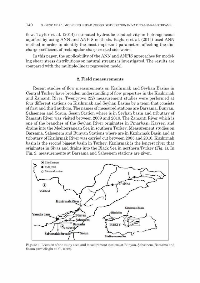
Recent studies of flow measurements on Kızılırmak and Seyhan Basins in Central Turkey have broaden understanding of flow properties in the Kızılırmak and Zamantı River. Twentytwo (22) measurement studies were performed at four different stations on Kızılırmak and Seyhan Basins by a team that consists of first and third authors. The names of measured stations are Barsama, Bünyan, Şahsenem and Sosun. Sosun Station where is in Seyhan basin and tributary of Zamantı River was visited between 2009 and 2010. The Zamantı River which is one of the branches of the Seyhan River originates in Pınarbaşı, Kayseri and drains into the Mediterranean Sea in southern Turkey. Measurement studies on Barsama, Şahsenem and Bünyan Stations where are in Kızılırmak Basin and at tributary of Kızılırmak River was carried out between 2005 and 2010. Kızılırmak basin is the second biggest basin in Turkey. Kızılırmak is the longest river that originates in Sivas and drains into the Black Sea in northern Turkey (Fig. 1). In Fig. 2, measurements at Barsama and Şahsenem stations are given.

Figure 1. Location of the study area and measurement stations at Bünyan, Şahsenem, Barsama and Sosun (Ardiclioglu et al., 2012).

GEOFIZIKA, VOL. 33, NO. 2, 2016, 137–156 141

Figure 2. Velocity and topographical measurements at (a) Barsama and (b) Şahsenem Stations (Ardiclioglu et al. 2012).

a)

b)

142 O. GENC ET AL.: MODELING SHEAR STRESS DISTRIBUTION IN NATURAL SMALL STREAMS ...

The technology of flow measurement devices has evolved rapidly in recent de-cades. Many flow measuring devices were discovered to determine the flow proper-ties. The Acoustic Doppler velocimeter, ADV which is one of these devices was uti-lized to measure three dimensional velocity data at the measured stations. The ADV is used to measure water velocity in a wide range of environments including laboratories, rivers, estuaries, and the ocean. An ADV operates by the principle of Doppler shift. All ADV measures the velocity samples by sending out short acous-tic waves from the transmitter probe. These waves travel to moving particulates in the liquid and three receiving probes record for the change in frequency of the re-turned waves. The velocity vector is transmitted to recorder of ADV. Three-dimensional flow velocities (u, v, w) for x, y, z directions can be measured by ADV in a sampling volume. Furthermore, ADV can be used to record one second velocity data for the specified averaging time, location, and water depth parameters (to document the data set), and a variety of statistical and quality control data. The ADV can measure sampling volume from 10 cm front of the probe head. Thus, the probe head itself does not much impact on the flow field surrounding the measure-ment volume. Velocity range is between ±0.001 m/s and 4.5 m/s, resolution 0.0001 m/s, accuracy ±1% of measured velocity (Sontek, 2002).

According to the water surface width (T), the stream is divided into segments for each field measurements. As seen in Tab. 1, wide channels (T / R ≥ 10) have 7–10 slices and narrow channels (T / R < 10) have 4–7 slices. Point velocity is mea-sured by ADV and cross-section area is measured using depth data measure-ments of distances from a fixed reference point on the riverbank. Point velocities were measured in the vertical direction starting 4 cm from the streambed for each vertical. Point velocity values were measured in the vertical direction start-ing 4 cm from the streambed for each vertical. Measurements were repeated ev-ery 2 cm from this point to water surface. The velocities of free water surface in all verticals were estimated using extrapolating the last two measurements of verticals. And also mean water surface velocities (uws) were measured at each visited stations. Water surface velocities were measured by how many seconds a tree branch passed distance of 10 meters using a chronometer. These measure-ments were repeated 10–15 times. In this way, we determined the average uws for all flow conditions and stations and given in the column 4 of Tab. 1.

The flow characteristics at each site are summarized in Tab. 1. As shown in Tab. 1, six measurements have been made at Barsama, Şahsenem and Bünyan stations in 2005–2006. Also, four measurement studies were undertaken at Sosun Station in 2009–2010.

The flow characteristics at each site are given in Tab. 1. In this table, first and second columns show visit numbers and dates of stations, Um (= Q / A) is the mean velocity, uws is the measured water surface velocity, with A being the area of the cross section, Hmax is the maximum flow depth, and T / R is the aspect ratio, with T being the surface water width, R (= A / P) is the hydraulic radius, P is

GEOFIZIKA, VOL. 33, NO. 2, 2016, 137–156 143

wetted perimeter. Re (= 4 Um R / u) is the Reynolds number, and u is the kinematic viscosity, Fr (= Um

/ (g Hmax)1/2) is the Froude number, where g is the gravitational acceleration, and S is water surface slope. According to the Froude and Reynolds numbers all the flow measurements are under subcritical and turbulent flow conditions according to Froude and Reynolds numbers. Froude numbers are be-tween 0.084–0.578, aspect ratios (T / R) vary between values 6.53–45.40. Reynolds numbers (Re × 106) vary between 0.32–1.47.

Table 1. Flow characteristics for all stations.

Stations Dates (dd/mm/year)

Um (m/s)

uws (m/s)

Hmax (m)

T (m) T/R Re

(×106) Fr S

Barsama_1 28/05/2005 0.890 1.60 39.0 8.3 34.00 0.76 0.481 0.0091

Barsama_2 19/05/2006 1.051 1.85 40.0 9.0 35.20 0.94 0.531 0.0036

Barsama_3 19/05/2009 1.214 2.08 45.0 9.0 29.70 1.47 0.578 0.0094

Barsama_4 31/05/2009 0.590 1.14 26.0 8.4 45.40 0.40 0.333 0.0092

Barsama_5 24/03/2010 0.806 1.55 38.0 8.6 34.40 0.61 0.417 0.0097

Barsama_6 18/04/2010 0.865 1.63 38.2 8.8 22.10 0.85 0.421 0.0120

Bünyan_1 24/06/2009 0.354 0.65 72.0 4.0 7.00 0.71 0.133 0.0020

Bünyan_2 08/02/2010 0.214 0.40 66.0 4.0 7.50 0.40 0.084 0.0030

Bünyan_3 27/09/2009 0.301 0.54 72.0 3.9 8.20 0.50 0.113 0.0022

Bünyan_4 04/04/2010 0.405 0.74 85.0 4.0 7.30 0.78 0.140 0.0018

Bünyan_5 16/05/2010 0.426 0.54 86.0 4.0 7.00 0.85 0.147 0,0024

Bünyan_6 20/06/2010 0.286 0.53 79.0 3.9 7.30 0.53 0.103 0.0010

Şahsenem_1 29/03/2006 0.600 1.04 28.0 6.0 26.80 0.47 0.350 0.0059

Şahsenem_2 20/10/2007 0.529 0.93 32.0 5.4 21.90 0.46 0.298 0.0061

Şahsenem_3 22/03/2008 0.565 0.80 33.0 6.0 22.10 0.49 0,314 0,0037

Şahsenem_4 03/05/2008 0.518 1.00 32.0 5.4 25.10 0.39 0.307 0.0045

Şahsenem_5 11/10/2008 0.536 1.01 32.0 5.5 22.00 0.44 0.303 0.0046

Şahsenem_6 08/11/2008 0.516 1.00 34.0 5.6 19.60 0.51 0.282 0.0064

Sosun_1 19/05/2009 0.561 0.96 62.0 3.2 7.49 0.84 0.227 0.0032

Sosun_2 31/05/2009 0.285 0,63 43.0 3.0 9,49 0.32 0.144 0.0016

Sosun_3 24/03/2010 0.327 0.63 45.0 2.9 8.85 0.37 0.156 0.0026

Sosun_4 18/04/2010 0.541 0.93 54.0 2.3 6.53 0.67 0.235 0.0034

144 O. GENC ET AL.: MODELING SHEAR STRESS DISTRIBUTION IN NATURAL SMALL STREAMS ...

Figure 3 presents the scatter plots for frequency histogram of 145 shear stress, 0 values in measured vertical. As seen from the figure, the most of shear stress, 0 values change between the values 0–20 N/m2. The minimum shear stress is 0.081 N/m2 and the maximum shear stress is 78.4 N/m2.

3. Shear stress distributions

Shear stress distribution basically depends upon the geometry of the cross section and the mechanism of the secondary flow cells. Shear force in uniform flow can be defined as in below

Ft = γ A L S (3)

where γ is the specific weight or unit weight of water, A is the channel cross sec-tional area, L is the length of the control volume and S is the longitudinal slope of the channel. Unit shear force is calculated using Eq. (3) as following form.

τγ

γ0 = =ALSPL

RS (4)

where, 0 is the average value of the shear force per unit of the wetted area, R is the hydraulic radius (= A / P in which A is the wetted area and P is wetted perimeter).

Figure 3. The frequency histograms of the target variable, shear stress 0.

Shear stress, 0 (N/m2)

Freq

uenc

y

GEOFIZIKA, VOL. 33, NO. 2, 2016, 137–156 145

It is clear that, shear force is not always uniformly distributed over the pe-rimeter. French (1985) stressed that for a sensitive calculation methodology to be determined, the distribution of the shear force on the perimeter of the channel should be predicted.

Schlicting (1987) informed that logarithmic relation between the shear veloc-ity and the variation of velocity with height is used to determine the local bed shear stress.

uu

zks* /

=

130χ

ln (5)

where u is stream wise velocity at z, u* = ( 0 / )1/2 is the shear velocity, is water density, ks is the Nikuradse’s original uniform sand grain roughness, is the von Kármán constant and z is distance from the bottom of the roughness elements.

4. Method

4.1. Artificial neural networks

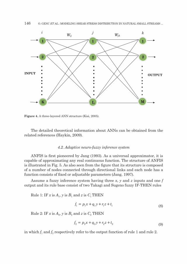
ANNs are developed by getting inspired from real nervous system by neglect-ing most of the biological details. They are massively parallel systems consisting many processing elements, called neurons. Each layer in ANNs is fully connected to the proceeding layer by interconnection weights. Figure 4 represents a three layered ANN comprising layers i, j, and k, with the weights Wij and Wjk between layers. Initial weight values are randomly assigned and then corrected during a training process. This process compares model outputs with measured outputs and back propagates any errors (from right to left in Fig. 4). Thus, the final weights are obtained by minimizing the errors (Kisi, 2005).

In layers j and k, each neuron receives the x input which is the weighted sum of outputs from the previous layer. As an example, in layer j, y can be given as

y W Opj ij pii

I

j= +=

∑1

θ (6)

in which qj is a bias for neuron j, Opi is ith output of the previous layer, Wij is the weights between the layers i and j. An output f(y) is obtained from each neuron in layers j and k by passing y value through a non-linear activation function. Logistic function is commonly used as an activation function

f ye y( )=

+ −

11

(7)

146 O. GENC ET AL.: MODELING SHEAR STRESS DISTRIBUTION IN NATURAL SMALL STREAMS ...

The detailed theoretical information about ANNs can be obtained from the related references (Haykin, 2009).

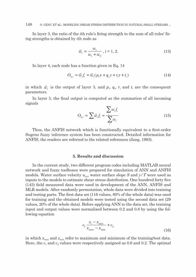
4.2. Adaptive neuro-fuzzy inference system

ANFIS is first pioneered by Jang (1993). As a universal approximator, it is capable of approximating any real continuous function. The structure of ANFIS is illustrated in Fig. 5. As also seen from the figure that its structure is composed of a number of nodes connected through directional links and each node has a function consists of fixed or adjustable parameters (Jang, 1997).

Assume a fuzzy inference system having three x, y and z inputs and one f output and its rule base consist of two Takagi and Sugeno fuzzy IF-THEN rules

Rule 1: IF x is A1, y is B1 and z is C1 THEN

f p x q y r z t1 1 1 1 1= + + + (8)

Rule 2: IF x is A2, y is B2 and z is C2 THEN

f p x q y r z t2 2 2 2 2= + + + (9)

in which f1 and f2 respectively refer to the output function of rule 1 and rule 2.

1

2

i

1

2

j

1

2

k Wjk

Wij

K L

INPUT OUTPUT

M

Figure 4. A three-layered ANN structure (Kisi, 2005).

GEOFIZIKA, VOL. 33, NO. 2, 2016, 137–156 147

Every node i in layer 1 includes an adaptive node function

O A xl i i, ( )=ϕ , for i = 1, 2 (10)

where x is the ith node’s input and Ai is a linguistic label such as “small” or “big” associated with this node function. Ol,i refers the membership function of a fuzzy set A (in this example; A1, A2, B1, B2, C1, or C2). It denotes the degree to which the given input x satisfies the Ai. Gaussian function is usually chosen for the A xi ( )

ϕA xx abi

i

i( ) exp= −

−

2

(11)

where ai and bi are the function’s parameters. When the values of these parame-ters change, the Gaussian function also varies accordingly, thus various forms of membership functions are exhibited on linguistic label Ai (Jang, 1993). The pa-rameters in this layer are named as premise parameters.

In layer 2, the incoming signals are multiplied in each node. For instance,

w A x B y C zi i i i=ϕ ϕ ϕ( ) ( ) ( ) , i = 1, 2. (12)

The output of each node indicates the firing strength of a rule.

Figure 5. The structure of an ANFIS.

1A x

y

x y z

w1

w2

1w

2w

11 fw

22 fw

f

Layer 1 Layer 2 Layer 3 Layer 4 Layer 5

2A

1B

2B

x y z

z C

C

N

N Σ

2

1

148 O. GENC ET AL.: MODELING SHEAR STRESS DISTRIBUTION IN NATURAL SMALL STREAMS ...

In layer 3, the ratio of the ith rule’s firing strength to the sum of all rules’ fir-ing strengths is obtained by ith node as

ww

w wii=

+1 2, i = 1, 2. (13)

In layer 4, each node has a function given in Eq. 14

O w f w p x q y r z ti i i i i i i i4, ( )= = + + + (14)

in which wi is the output of layer 3, and pi, qi, ri and ti are the consequent parameters.

In layer 5, the final output is computed as the summation of all incoming signals

O w fw f

wi i i

i ii

ii

5, = =

∑

∑∑ (15)

Thus, the ANFIS network which is functionally equivalent to a first-order Sugeno fuzzy inference system has been constructed. Detailed information for ANFIS, the readers are referred to the related references (Jang, 1993).

5. Results and discussion

In the current study, two different program codes including MATLAB neural network and fuzzy toolboxes were prepared for simulation of ANN and ANFIS models. Water surface velocity uws, water surface slope S and y / T were used as inputs to the models to estimate shear stress distribution. One hundred forty five (145) field measured data were used in development of the ANN, ANFIS and MLR models. After randomly permutation, whole data were divided into training and testing parts. The first data set (116 values, 80% of the whole data) was used for training and the obtained models were tested using the second data set (29 values, 20% of the whole data). Before applying ANN to the data set, the training input and output values were normalized between 0.2 and 0.8 by using the fol-lowing equation

c

x xx x

ci1 2

−

−+min

max min (16)

in which xmax and xmin refer to maximum and minimum of the training/test data. Here, the c1 and c2 values were respectively assigned as 0.6 and 0.2. The optimal

GEOFIZIKA, VOL. 33, NO. 2, 2016, 137–156 149

ANN models were obtained after trying various model structures. The evaluat-ing criteria used in the study are root mean square errors (RMSE), mean abso-lute errors (MAE) and determination coefficient (R2). The equations of the RMSE, MAE and R2 are:

MSE

Nx yi

i

N

= −( )=

∑1 2

1i

(17)

RMSE MSE (18)

MAE

Nx yi

i

n

= −=

∑11

i (19)

Rx x y y

x x y y

i ii

n

i ii

n

i

n2 1

2

2 2

11

=

−( ) −( )

−( ) −( )

=

==

∑

∑∑ (19)

where N and yi refer to number of data set and entropy parameter, respectively. MSE is mean square errors.

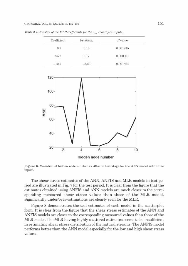
For estimating shear stress distribution of the streams, three different input combinations were used. The Pearson correlations between the inputs uws, S, y / T and output are 0.804, 0.772 and 0.031, respectively. The lowest linear relation-ship exists between the y / T and output and the uws has the highest correlation. According to the correlation values, uws seems to be the most effective variable on shear stress distribution. The optimal hidden node numbers were obtained for each ANN model by using simple trial and error method. The hidden node num-ber tried for each ANN model ranges between 1 and 10. As an example, the vari-ation of hidden node number vs. mean square error (MSE) in test stage for the ANN model with three inputs is illustrated in Fig. 6. The ANN models were trained by using Conjugate Gradient algorithm which is more powerful than the classical gradient descent technique. The sigmoid activation functions were used for the hidden and output nodes. The ANN training was stopped after 1000 itera-tions. Training and test results of the optimal ANN models are shown in Tab. 2 in respect of RMSE, MAE and R2 statistics. The optimal hidden node numbers are also provided in the second column of this table. It is apparent from the table that the ANN model comprising three inputs corresponding to uws, Sws and y / T, 6 hidden and 1 output nodes has the lowest RMSE, MAE and the highest R2 both in training and test periods. From Tab. 2, it is clear that the accuracy of ANN

150 O. GENC ET AL.: MODELING SHEAR STRESS DISTRIBUTION IN NATURAL SMALL STREAMS ...

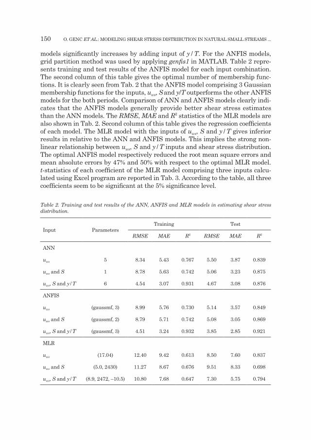
models significantly increases by adding input of y / T. For the ANFIS models, grid partition method was used by applying genfis1 in MATLAB. Table 2 repre-sents training and test results of the ANFIS model for each input combination. The second column of this table gives the optimal number of membership func-tions. It is clearly seen from Tab. 2 that the ANFIS model comprising 3 Gaussian membership functions for the inputs, uws, S and y/T outperforms the other ANFIS models for the both periods. Comparison of ANN and ANFIS models clearly indi-cates that the ANFIS models generally provide better shear stress estimates than the ANN models. The RMSE, MAE and R2 statistics of the MLR models are also shown in Tab. 2. Second column of this table gives the regression coefficients of each model. The MLR model with the inputs of uws, S and y / T gives inferior results in relative to the ANN and ANFIS models. This implies the strong non-linear relationship between uws, S and y / T inputs and shear stress distribution. The optimal ANFIS model respectively reduced the root mean square errors and mean absolute errors by 47% and 50% with respect to the optimal MLR model. t-statistics of each coefficient of the MLR model comprising three inputs calcu-lated using Excel program are reported in Tab. 3. According to the table, all three coefficients seem to be significant at the 5% significance level.

Table 2. Training and test results of the ANN, ANFIS and MLR models in estimating shear stress distribution.

Input ParametersTraining Test

RMSE MAE R2 RMSE MAE R2

ANN

uws 5 8.34 5.43 0.767 5.50 3.87 0.839

uws and S 1 8.78 5.63 0.742 5.06 3.23 0.875

uws, S and y / T 6 4.54 3.07 0.931 4.67 3.08 0.876

ANFIS

uws (gaussmf, 3) 8.99 5.76 0.730 5.14 3.57 0.849

uws and S (gaussmf, 2) 8.79 5.71 0.742 5.08 3.05 0.869

uws, S and y / T (gaussmf, 3) 4.51 3.24 0.932 3.85 2.85 0.921

MLR

uws (17.04) 12.40 9.42 0.613 8.50 7.60 0.837

uws and S (5.0, 2430) 11.27 8.67 0.676 9.51 8.33 0.698

uws, S and y / T (8.9, 2472, –10.5) 10.80 7.68 0.647 7.30 5.75 0.794

GEOFIZIKA, VOL. 33, NO. 2, 2016, 137–156 151

Table 3. t-statistics of the MLR coefficients for the uws, S and y/T inputs.

Coefficient t-statistic P value

8.9 3.18 0.001915

2472 5.17 0.000001

–10.5 –3.30 0.001824

Figure 6. Variation of hidden node number vs MSE in test stage for the ANN model with three inputs.

The shear stress estimates of the ANN, ANFIS and MLR models in test pe-riod are illustrated in Fig. 7 for the test period. It is clear from the figure that the estimates obtained using ANFIS and ANN models are much closer to the corre-sponding measured shear stress values than those of the MLR model. Significantly under/over-estimations are clearly seen for the MLR.

Figure 8 demonstrates the test estimates of each model in the scatterplot form. It is clear from the figure that the shear stress estimates of the ANN and ANFIS models are closer to the corresponding measured values than those of the MLR model. The MLR having highly scattered estimates seems to be insufficient in estimating shear stress distribution of the natural streams. The ANFIS model performs better than the ANN model especially for the low and high shear stress values.

152 O. GENC ET AL.: MODELING SHEAR STRESS DISTRIBUTION IN NATURAL SMALL STREAMS ...

0102030405060

0 10 20 30

Shea

r str

ess

dist

ribu

tion

Measurements

Measured ANN

0102030405060

0 10 20 30

Shea

r str

ess

dist

ribu

tion

Measurements

Measured ANFIS

0102030405060

0 10 20 30

Shea

r str

ess

dist

ribu

tion

Measurements

Measured MLR

Figure 7. Time variation of the measured and estimated shear stress values by ANN, ANFIS and MLR models.

GEOFIZIKA, VOL. 33, NO. 2, 2016, 137–156 153

The results are tested by using one way ANOVA for verifying the robustness (the significance degree of differences between the model estimates and mea-sured shear stress distribution) of the models. The test is set at a 95% significant level. Table 4 reports the test statistics. It is clear from the table that the ANFIS and ANN models yield small testing values with high significance levels. From Table 4, the ANFIS and ANN models seem to be more robust (the similarity be-tween the measured entropy parameters and model estimates are significantly high) in shear stress estimation than the MLR model.

Table 4. ANOVA of ANFIS, ANN and MLR models in the test period.

Model F-statistic Resultant significance levelANFIS(gaussmf, 3 ) 0.024 0.878ANN(3,6,1) 0.020 0.889MLR 0.302 0.585

Figure 8. The scatterplots of the measured and estimated shear stress values by ANN, ANFIS and MLR models.

y = 0.8696x + 0.9565R² = 0.8756

0

10

20

30

40

50

60

0 10 20 30 40 50 60

ANN

Measured

y = 0.8541x + 1.0867R² = 0.9212

0

10

20

30

40

50

60

0 10 20 30 40 50 60

ANFI

S

Measured

y = 0.5317x + 6.7339R² = 0.794

0

10

20

30

40

50

60

0 10 20 30 40 50 60

MLR

Measured

y = 0.8696x + 0.9565R² = 0.8756

0

10

20

30

40

50

60

0 10 20 30 40 50 60

ANN

Measured

y = 0.8541x + 1.0867R² = 0.9212

0

10

20

30

40

50

60

0 10 20 30 40 50 60

ANFI

S

Measured

y = 0.5317x + 6.7339R² = 0.794

0

10

20

30

40

50

60

0 10 20 30 40 50 60

MLR

Measured

154 O. GENC ET AL.: MODELING SHEAR STRESS DISTRIBUTION IN NATURAL SMALL STREAMS ...

6. Conclusion

This study investigated the accuracy of ANFIS and ANN methods for esti-mating shear stress distribution in streams. Overall 145 field data gauged from four different cross-sections at four sites on the Sarımsaklı and Sosun streams in Turkey were used. The water surface velocity uws, water surface slope S and y / T were used as inputs to the ANFIS and ANN models for estimating shear stress distribution. The estimates obtained from the ANFIS and ANN models were compared with multiple-linear regression model. The results revealed that the ANFIS and ANN models performed much better than the MLR model in esti-mating shear stress distribution. The ANFIS was found to be slightly better than the ANN. The best ANFIS model was respectively reduced the root mean square errors and mean absolute errors by 47% and 50% with respect to the best MLR model. The study recommends that the ANFIS and ANN techniques can be suc-cessfully used for estimating shear stress distribution of the natural streams.

References

Ardiclioglu, M., Seckin, G. and Yurtal, R. (2006): Shear stress distributions along the cross section in smooth and rough open channel flows, Kuwait J. Sci. Eng., 33, 155–168.

Ardiclioglu, M., Genc, O., Kalin, L. and Agiralioglu, N. (2012): Investigation of flow properties in natural streams using the entropy concept, Water Environ. J., 26, 147–154, DOI: 10.1111/ j.1747-6593.2011.00270.x.

Berlamont, J. E., Trouw, K. and Luyckx, G. (2003): Shear stress distribution in partially filled pipes, J. Hydraul. Eng.-ASCE, 129, 697–705, DOI: 10.1061/(ASCE)0733-9429(2003)129:9(697).

Bilhan, O., Emiroglu, M. E. and Kisi, O. (2010): Application of two different neural network techniques to lateral outflow over rectangular side weirs located on a straight channel, Adv. Eng. Softw., 41, 831–837, DOI: 10.1016/j.advengsoft.2010.03.001.

Cacqueray, N., Hargreaves, D. M. and Morvan, H. P. (2009): A computational study of shear stress in smooth rectangular channels, J. Hydraul. Res., 47, 50–57, DOI: 10.3826/jhr.2009.3271.

Can, I., Tosunoglu, F. and Kahya, E. (2012): Daily streamflow modelling using autoregressive moving av-erage and artificial neural networks models: case study of Çoruh basin, Turkey, Water Environ. J., 26, 567–576, DOI: 10.1111/j.1747-6593.2012.00337.x.

Christensen, B. and Fredsoe, J. (1998): Bed shear stress distribution in straight channels with arbitrary cross section, Progress Rep. 77. Dept. of Hydrodynamics and Water Resources, TU Denmark, Lyngby.

Cobaner, M., Seckin, G. and Kisi, O. (2008): Initial assessment of bridge backwater using artificial neural network approach, Can. J. Civil Eng., 35, 500–510.

Cobaner, M., Seckin, G., Seckin, N. and Yurtal, R. (2010): Boundary shear stress analysis in smooth rect-angular channels and ducts using neural networks, Water Environ. J., 24, 133–139, DOI: 10.1111/ j.1747-6593.2009.00165.x.

Dogan, E., Yuksel, I. and Kisi, O. (2007): Estimation of total sediment load concentration obtained by ex-perimental study using artificial neural networks, Environ. Fluid Mech., 7, 271–288, DOI: 10.1007/s10652-007-9025-8.

GEOFIZIKA, VOL. 33, NO. 2, 2016, 137–156 155

Dursun, O. F., Kaya, N. and Firat, M. (2012): Estimating discharge coefficient of semi-elliptical side weir using ANFIS, J. Hydrology, 426–427, 55–62, DOI: 10.1016/j.jhydrol.2012.01.010.

French, R. H. (1985): Open-Channel Hydraulics. McGraw-Hill Inc., New York, 620 pp.Ghosh, S. N. and Roy, N. (1970): Boundary shear distribution in open channel flow, J. Hydraulics Div. –

Proc. ASCE, 96, 967–994.Guven, A. (2011): A multi-output descriptive neural network for estimation of scour geometry down-

stream from hydraulic structures, Adv. Eng. Softw., 42, 85–93, DOI: 10.1016/j.advengsoft. 2010.12.005.

Haykin, S. (2009): Neural Networks and Learning Machines. Prentice Hall, New Jersey, 906 pp.Hicks, F. E., Jin, Y. C. and Steffler, P. M. (1990): Flow near sloped bank in curved channel, J. Hydraul.

Eng.-ASCE, 116, 55–70, DOI: 10.1061/(ASCE)0733-9429(1990)116:1(55).Jang, J. S. R. (1993): ANFIS: Adaptive-network-based fuzzy inference system, IEEE T. Syst. Man Cybern.,

23, 665–685, DOI: 10.1109/21.256541.Jang, J. S. R., Sun, C. T. and Mizutani, E. (1997): Neuro-Fuzzy and Soft Computing: A Computational

Approach to Learning and Machine Intelligence. Prentice Hall, New Jersey, 614 pp.Khodashenas, S. R., Abderrezzak, K. K. and Paquier, A. (2008): Boundary shear stress in open channel

flow: A comparison among six methods, J. Hydraul. Res., 46, 598–609, DOI: 10.3826/jhr.2008.3203.Kisi, O. (2005): Suspended sediment estimation using neuro-fuzzy and neural network approaches,

Hydrol. Sci. J., 50, 683–696, DOI: 10.1623/hysj.2005.50.4.683.Kisi, O., Bilhan, O. and Emiroglu, M. E. (2013): ANFIS to estimate discharge capacity of rectangular side

weir, P. I. Civil Eng.-Wat. M., 166, 479–487, DOI: 10.1680/wama.11.00095.Knight, D. W. and Patel, H. S. (1985): Boundary shear in smooth rectangular ducts, J. Hydraul. Eng.-

ASCE, 111, 29–47, DOI: 10.1061/(ASCE)0733-9429(1985)111:1(29).Knight, D. W., Yuen, K. W. H. and Alhamid, A. A. I. (1994): Boundary shears stress distributions in open

channel flow, in: Physical mechanisms of mixing and transport in the environment, edited by Beven, K., Chatwin, P. and Millbank, J. Wiley, New York, 51–87.

Knight, D. W., Demetriou, J. D. and Hamed, M. E. (1984): Boundary shear in smooth rectangular chan-nels, J. Hydraul. Eng.-ASCE, 110, 405–422, DOI: 10.1061/(ASCE)0733-9429(1984)110:4(405).

Kocabas, U. and Ülker, S. (2006): Estimation of critical submergence for an intake in a stratified fluid media by neuro-fuzzy approach, Environ. Fluid Mech., 6, 489–500, DOI: 10.1007/s10652-006-9005-4.

Kocabas, F., Kisi, O. and Ardiclioglu, M. (2009): An artificial neural network model for prediction of criti-cal submergence for an intake in a stratified fluid media, Civ. Eng. Environ. Syst., 26, 367–375, DOI: 10.1080/10286600802200130.

Lundgren, H. and Johnson, I. G. (1964): Shear and velocity distribution in shallow channels, J. Hydr. Div., 90, 1–21.

Mamak, M., Seckin, G., Cobaner, M. and Kisi, O. (2009): Bridge afflux analysis through arched bridge constrictions using artificial intelligence methods, Civ. Eng. Environ. Syst., 26, 279–793, DOI: 10.1080/10286600802151804.

Marsili-Libelli, S., Giusti, E. and Nocita, A. (2013): A new instream flow assessment method based on fuzzy habitat suitability and large scale river modelling, Environ. Model. Softw., 41, 27–38, DOI: 10.1016/j.envsoft.2012.10.005.

Mohammadi, M. and Knight, D. W. (2004): Boundary shear stress distribution in a V-shaped channel, in: Hydraulics of Dams and River Structures, edited by Yazdandoost, F. and Attari, J., Taylor & Francis Group, London, 401–410.

Rezaeianzadeh, M., Tabari, H., Yazdi, A. A., Isik, S. and Kalin, L. (2013): Flood flow forecasting using ANN, ANFIS and regression models, Neural Comput. Applic., 25, 25–37, DOI 10.1007/s00521-013-1443-6.

156 O. GENC ET AL.: MODELING SHEAR STRESS DISTRIBUTION IN NATURAL SMALL STREAMS ...

Riahi-Madvar, H., Ayyoubzadeh, S. A., Khadangi, E. and Ebadzadeh, M. H. (2009): An expert system for predicting longitudinal dispersion coefficient in natural streams by using ANFIS, Exp. Syst. Appl., 36, 8589–8596, DOI: 10.1016/j.eswa.2008.10.043.

Schlicting, H. (1987): Boundary Layer Theory. McGraw-Hill, New York, pp 525–529. SonTek (2002): Flow Tracker Handheld ADV, Technical Document, available at ftp://ksh.fgg.uni-lj.si/stu-

dents/podipl/merska_oprema/Flow_Tracker_Manual.pdf.Tayfur, G., Nadiri, A. A. and Moghaddam, A. A. (2014): Supervised intelligent committee machine meth-

od for hydraulic conductivity estimation, Water Resour. Manage., 28, 1173–1184, DOI: 10.1007/s11269-014-0553-y.

Tracy, H. J. (1965): Turbulent flow in a three-dimensional channel, J. Hydraulics Div.–Proc. ASCE, 91(6), 9–35.

Wolfs, V. and Willems, P. (2013): A data driven approach using Takagi–Sugeno models for computation-ally efficient lumped floodplain modelling, J. Hydrol., 503, 222–232, DOI: 10.1016/j.jhydrol. 2013.08.020.

Yang, S. Q. and Lim, S. Y. (2005): Boundary shear stress distributions in trapezoidal channels, J. Hydraulic Res., 43, 98–102, DOI: 10.1080/00221680509500114.

Yang, H. C. and Chang, F. J. (2005): Modelling combined open channel flow by artificial neural networks, Hydro. Process, 19, 3747–3762, DOI: 10.1002/hyp.5858.

Yu, G. and Tan, S. K. (2007): Estimation of boundary shear stress distribution in open channels using flownet, J. Hydraul. Res., 45, 486–496, DOI: 10.1080/00221686.2007.9521783.

Zheng, Y. and Jin, Y. C. (1998): Boundary shear in rectangular ducts and channels, J. Hydraul. Eng.-ASCE, 124, 86–89, DOI: 10.1061/(ASCE)0733-9429(1998)124:1(86).

SAŽETAK

Modeliranje razdiobe napetosti smicanja u prirodnim malim vodotocima metodama mekog računanja

Onur Genc, Ozgur Kisi i Mehmet Ardiclioglu

U ovoj studiji su za procjenu razdiobe napetosti smicanja u vodotocima korištene umjetne neuronske mreže (ANNs) i prilagodljivi neizraziti sustav zaključivanja (ANFIS). Metode su primijenjene na 145 nizova podataka prikupljenih na četiri različite postaje na vodotocima Sarimsakli i Sosun u Turskoj. Točnost primijenjenih modela uspoređena je s točnošću modela višestruke linearne regresije (MLR). Rezultati su pokazali da su oba mo-dela (ANNs i ANFIS) bili bolji u modeliranju raspodjele napetosti smicanja od MLR mode-la. Pri korištenju ANFIS modela za procjenu raspodjele napetosti smicanja u testnom raz-doblju srednje kvadratne pogreške (RMSE) i srednje apsolutne pogreške (MAE) su u odnosu na MLR model bile smanjene za 47%, odnosno 50%. Utvrđeno je da se za testno razdoblje najbolji ANFIS model, s RMSE = 3,85, MAE = 2,85 i koeficijentom određenosti R2 = 0.921, pokazao superiornim u procjeni napetosti smicanja u odnosu na MLR model, s RMSE = 7,30, MAE = 5,75 i R2 = 0.794.

Ključne riječi: ANN, ANFIS, linearna regresija, napetost smicanja, vodotok, turbulentni tok

Corresponding author’s address: Ozgur Kisi, International Black Sea University, Tbilisi, Georgia; tel: +90 362 280 1081; email: okisi@ibsu.edu.ge