Modeling, Optimization, and Detailed Design of a Hydraulic ...

Modeling, Optimization, and Detailed Design of a Hydraulic

Flywheel-Accumulator

A THESIS

SUBMITTED TO THE FACULTY OF THE

UNIVERISTY OF MINNESOTA

BY

Kyle Glenn Strohmaier

IN PARTIAL FULFILLMENT OF THE REQUIREMENTS

FOR THE DEGREE OF

MASTER OF SCIENCE

Adviser: James Van de Ven, Ph.D.

July 2014

i

I would like to thank my adviser, Dr. James Van de Ven, for providing me the

opportunity to partake in this fascinating research and for his guidance and patience

throughout the process.

This work was sponsored by the National Science Foundation through the Center for

Compact and Efficient Fluid Power, grant EEC-0540834.

ii

Abstract

Improving mobile energy storage technology is an important means of addressing

concerns over fossil fuel scarcity and energy independence. Traditional hydraulic

accumulator energy storage, though favorable in power density, durability, cost, and

environmental impact, suffers from relatively low energy density and a pressure-

dependent state of charge. The hydraulic flywheel-accumulator concept utilizes both the

hydro-pneumatic and rotating kinetic energy domains by employing a rotating pressure

vessel. This thesis provides an in-depth analysis of the hydraulic flywheel-accumulator

concept and an assessment of the advantages it offers over traditional static accumulator

energy storage.

After specifying a practical architecture for the hydraulic flywheel-accumulator, this

thesis addresses the complex fluid phenomena and control implications associated with

multi-domain energy storage. To facilitate rapid selection of the hydraulic flywheel-

accumulator dimensions, computationally inexpensive material stress models are

developed for each component. A drive cycle simulation strategy is also developed to

assess the dynamic performance of the device. The stress models and performance

simulation are combined to form a toolset that facilitates computationally-efficient

model-based design.

The aforementioned toolset has been embedded into a multi-objective optimization

algorithm that aims to minimize the mass of the hydraulic flywheel-accumulator system

and to minimize the losses it incurs over the course of a drive cycle. Two optimizations

have been performed – one with constraints that reflect a vehicle-scale application, and

one with constraints that reflect a laboratory application. At both scales, the optimization

results suggest that the hydraulic flywheel-accumulator offers at least an order of

magnitude improvement over traditional static accumulator energy storage, while

operating at efficiencies between 75% and 93%. A particular hydraulic flywheel-

accumulator design has been selected from the set of laboratory-scale optimization results

and subjected to a detailed design process. It is recommended that this selection be

constructed and tested as a laboratory prototype.

iii

Table of Contents

List of Tables .......................................................................................................................... vi

List of Figures ....................................................................................................................... viii

1 Introduction .............................................................................................................................. 1

1.1 Greenhouse Gas Emissions and Traditional Vehicles ..................................................... 1

1.2 Alternative Powertrains ................................................................................................... 2

1.3 Hydraulic Powertrain Components .................................................................................. 5

1.4 The Hydraulic Flywheel-Accumulator Concept .............................................................. 8

1.5 Research Goals and Approach ....................................................................................... 10

2 General Architecture and Operation ...................................................................................... 12

2.1 Architecture and Design Variables of the Hydraulic Flywheel-Accumulator ............... 12

2.2 Basic Kinetic and Pneumatic Energy Storage ................................................................ 17

2.3 Fluid Centrifugation ....................................................................................................... 19

2.4 Interaction of the Energy Storage Domains ................................................................... 22

2.5 Controlling the Hydraulic Flywheel-Accumulator ........................................................ 24

2.6 Optimization Objectives and Constraints ...................................................................... 27

3 Model-Based Structural Design ............................................................................................. 29

3.1 System-Level Considerations ........................................................................................ 29

3.2 Axle ................................................................................................................................ 34

3.3 End Caps ........................................................................................................................ 41

3.4 Piston ............................................................................................................................. 45

3.5 Housing .......................................................................................................................... 50

3.6 Bearing Selection ........................................................................................................... 58

3.7 Material Selection and Static Calculations .................................................................... 64

4 Energy Loss Mechanisms ...................................................................................................... 67

4.1 Bearing and Aerodynamic Drag .................................................................................... 68

4.2 Storage Pump-Motor Losses .......................................................................................... 72

4.3 Losses Related to the High-Speed Rotary Union ........................................................... 75

4.4 Vacuum Pumping Energy Consumption ........................................................................ 81

5 Internal Fluid Modeling ......................................................................................................... 86

5.1 Motivation for Fluid Modeling ...................................................................................... 86

iv

5.2 Theory and Assumptions ............................................................................................... 88

5.3 Modeling Approach ....................................................................................................... 94

5.4 Experimental Approach ................................................................................................. 96

5.5 Model Development ..................................................................................................... 102

5.6 Model Validation ......................................................................................................... 109

5.7 Closing Remarks about the Internal Fluid Modeling ................................................... 116

6 Drive Cycle Simulation ........................................................................................................ 118

6.1 Road Loads and Vehicle Parameters ........................................................................... 118

6.2 Control Strategy and Pump-Motor Selection ............................................................... 121

6.3 Studies on the Band Control Strategy Parameters ....................................................... 125

6.4 Calculation Sequence ................................................................................................... 132

6.5 Calculation of Performance Metrics ............................................................................ 139

7 Design Optimization ............................................................................................................ 141

7.1 Optimization Strategy .................................................................................................. 141

7.2 Posing the Optimization Problem ................................................................................ 144

7.3 Vehicle-Scale Optimization Results ............................................................................ 147

7.4 Laboratory-Scale Optimization Results ....................................................................... 159

7.5 Contextualizing the Optimization Results ................................................................... 168

7.6 Selection of a Design Solution for the Laboratory Prototype ...................................... 174

8 Detailed Design .................................................................................................................... 179

8.1 Torque Transmission Mechanisms .............................................................................. 179

8.2 End Caps ...................................................................................................................... 184

8.3 Piston ........................................................................................................................... 197

8.4 Housing ........................................................................................................................ 201

8.5 Axle .............................................................................................................................. 205

8.6 High-Speed Rotary Union Case ................................................................................... 208

8.7 Relative Radial Strain Analysis ................................................................................... 213

9 Conclusions and Recommendations .................................................................................... 221

9.1 Summary of the Research ............................................................................................ 221

9.2 Conclusions .................................................................................................................. 222

9.3 Future Work ................................................................................................................. 224

Bibliography ........................................................................................................................ 227

Appendix A: Nomenclature ................................................................................................. 233

v

Appendix B: MATLAB© Code for the Model-based Design and Simulation Toolset ........ 240

Appendix C: Complete Experimental Results from the Fluid Behavior Model Development

............................................................................................................................................. 286

Appendix D: Simulated Prototype Performance .................................................................. 320

Appendix E: Additional FEA Results .................................................................................. 324

vi

List of Tables

Table 1: The Nine Design Variables which Constitute a Design Solution for the HFA ................ 16

Table 2: Load Cases for a Study on Stresses in a Hybrid Housing ................................................ 54

Table 3: Selected Materials and their Mechanical Properties [45] ................................................ 65

Table 4: Properties of the Composite Material for the Housing Wrap [35] ................................... 66

Table 5: List of Energy Loss Mechanisms and their Symbols (Given as Rates of Energy

Dissipation), Categorized as Kinetic or Pneumatic ....................................................................... 67

Table 6: Volumetric and Mechanical Efficiency Definitions for Pumping and Motoring ............ 73

Table 7: Selected Loss Coefficients for the Storage Pump-Motor [54] ......................................... 74

Table 8: Selected Values for the Minor Loss Coefficients in the Axial Ports ............................... 77

Table 9: Minor Loss Coefficients in Pneumatic Charging and Discharging ................................. 77

Table 10: Assumptions for the Reduction of the Navier-Stokes Equations for Flow in the

Circumferential Seal ...................................................................................................................... 79

Table 11: General Specifications for the Experimental Setup ....................................................... 97

Table 12: Specifications of the Equipment Used for the Experimental Setup ............................... 98

Table 13: Ranked Performance of the Viscous Dissipation Rate Correlations, Based on

Coefficient of Determination ....................................................................................................... 105

Table 14: Ranked Performance of the Dynamic Time Constant Correlations, Based on Coefficient

of Determination .......................................................................................................................... 107

Table 15: Characteristics of the Urban Dynamometer Driving Schedule (UDDS) ..................... 119

Table 16: Vehicle Characteristics for Drive Cycle Simulation, Selected to Represent a Typical

Mid-Size Passenger Sedan ........................................................................................................... 121

Table 17: HFA Design Solution for the Control Strategy Study ................................................. 128

Table 18: Selected Control Strategy Parameter Values for the Control Strategy Study .............. 128

Table 19: Summary of the Genetic Algorithm Parameters .......................................................... 143

Table 20: Redefined Design Solution, Used for the Purposes of a Design Optimization ............ 145

Table 21: Design Variable Bounds for the Design Optimization ................................................ 146

Table 22: Summary of the Extreme Pareto-optimal Solutions from the Vehicle-Scale

Optimization ................................................................................................................................ 149

Table 23: Summary of the Extreme Pareto-optimal Solutions from the Laboratory-Scale

Optimization ................................................................................................................................ 163

Table 24: Results of the Energy Density Comparison Study ....................................................... 170

Table 25: Design Variable Values for the Selected Laboratory Prototype Design ...................... 176

Table 26: Non-design Variables of Interest for the Selected Laboratory Prototype Design ........ 177

Table 27: Static Performance Metrics for the Selected Laboratory Prototype Design ................ 178

Table 28: Drive Cycle (UDDS) Performance Metrics for the Selected Laboratory Prototype

Design .......................................................................................................................................... 178

Table 29: Selected Shoulder Screws for the Pin System ............................................................. 182

Table 30: The Three Potential Worst-case Loading Scenarios for the Housing .......................... 202

Table 31: Loads and Radial Displacements for the Worst-case Leakage Scenario at the Axle-

Piston Interface ............................................................................................................................ 215

vii

Table 32: Loads and Radial Displacements for the Worst-case Binding Scenario at the Axle-

Piston Interface ............................................................................................................................ 216

Table 33: Loads and Radial Displacements for the Worst-case Leakage Scenarios at the Piston-

Housing Interface ......................................................................................................................... 217

Table 34: Loads and Radial Displacements for the Worst-case Binding Scenarios at the Piston-


Table 35: Loads and Radial Displacements for the Worst-case Leakage Scenario at the Axle-End

Cap Interface ................................................................................................................................ 219

Table 36: Loads and Radial Displacements for the Worst-case Leakage Scenarios at the End Cap-


viii

List of Figures

Figure 1: Global Greenhouse Gas Emissions by Sector [1] ............................................................. 2

Figure 2: The Two Most Basic Hybrid Vehicle Powertrain Architectures, Series and Parallel. The

ICE and secondary energy storage-conversion pairs are labelled “A” and “B,” respectively. ........ 3

Figure 3: Illustration of a Traditional Piston-type Hydraulic Accumulator [17] ............................. 6

Figure 4: Dimensionless Pressure as a Function of Dimensionless Energy for a Traditional

Accumulator ..................................................................................................................................... 7

Figure 5: Pure Hydraulic Powertrain with a Hydraulic Flywheel Accumulator as the Sole Energy

Storage Medium. Shown with a Fixed-Displacement Storage Pump-Motor .................................. 9

Figure 6: Illustration of the Parabolic Oil Pressure Distribution with System Pressure at the

Vertex (Gas Pressure Distribution Not Shown) ............................................................................. 10

Figure 7: Hybrid Housing, Made of Metallic Liner and Composite Wrap .................................... 13

Figure 8: End Cap and Axle System .............................................................................................. 14

Figure 9: Illustration of the Spatial Relations between the Piston, Axle and End Caps ................ 14

Figure 10: Schematic of the High-Speed Rotary Union (HSRU) Concept .................................... 15

Figure 11: Force Balance on an Infinitesimal Fluid Element in a Rotating Fluid Volume [23] .... 19

Figure 12: Qualitative Illustration of the Gas (Left) and Oil (Right) Pressure Distributions for

Different Angular Velocities, with the Arrows Indicating Increasing Angular Velocity .............. 22

Figure 13: Sign Convention for Tractive (Total) Power, Power in the Kinetic Domain, and Power

in the Pneumatic Domain ............................................................................................................... 24

Figure 14: Three Possible Mounting Orientations for the HFA, Showing Forces that Contribute to

Bearing Loads ................................................................................................................................ 30

Figure 15: Illustration of the HFA Mounting Architecture ............................................................ 31

Figure 16: Exploded View of the Retaining Ring System for Torque Transmission between the

Axle and End Caps......................................................................................................................... 32

Figure 17: Illustration of the Pins (As Shown, 𝑵𝒔𝒔 = 𝟐) which Produce an Axial and Tangential

Constraint between the Housing and the Gas Side End Cap ......................................................... 33

Figure 18: Axle Dimensions .......................................................................................................... 34

Figure 19: Free Body Diagram of the Major Loads on the Axle-End Cap System ....................... 35

Figure 20: Free Body Diagram (Excluding Radial Forces) of the Lower Portion of the Axle ...... 37

Figure 21: Loading on the Portion of Axle that Forms the Circumferential Seal .......................... 39

Figure 22: Pressure Loading on the Oil Side End Cap (Retainer Pressure 𝑷𝒓 Acts on the

Counterbore Surface) ..................................................................................................................... 43

Figure 23: Piston Design ................................................................................................................ 46

Figure 24: Packaging Region of the Piston Seals .......................................................................... 46

Figure 25: Maximum von Mises Stress (Non-dimensionalized) for the Same System Pressure at

Different Angular Velocities; Two Piston Geometries Shown ...................................................... 48

Figure 26: Oil, Gas, and Net Pressure Distributions for Three Different Angular Velocities which

Produce the Same Maximum von Mises Stress for a Given HFA Geometry and System Pressure

....................................................................................................................................................... 49

Figure 27: Non-dimensional Radial and Circumferential Stress Distributions due to

Centrifugation of an Isotropic Hollow Cylinder ............................................................................ 51

ix

Figure 28: Hybrid Rotor Load Case 1 - Unpressurized at High Speed .......................................... 55

Figure 29: Hybrid Rotor Load Case 2 - Pressurized at High Speed .............................................. 56

Figure 30: Hybrid Rotor Load Case 3 - Pressurized at Zero Speed ............................................... 57

Figure 31: Normal and Torsional Stress Concentration Factors Used in the Axle Shaft Stress

Calculations ................................................................................................................................... 61

Figure 32: Plots Used to Determine e and Y Values for Calculating Equivalent Bearing Load .... 63

Figure 33: Axle Flow Passages, Shown with Oil Flowing Into the HFA ...................................... 75

Figure 34: Actual Flow Geometry for Non-contacting Circumferential Seal, Shown with

Exaggerated Clearance ................................................................................................................... 78

Figure 35: Semi-Infinite Planar Approximation of Non-contacting Circumferential Seal Flow

Geometry ....................................................................................................................................... 79

Figure 36: Schematic of the Containment Chamber Packaging .................................................... 83

Figure 37: Container and fluid volume with dimensions ............................................................... 88

Figure 38: Experimental Setup with Instrumentation .................................................................... 97

Figure 39: Example of an Attempted Step Change from 200 RPM to 1000 RPM, Desired and

Achieved ........................................................................................................................................ 99

Figure 40: Example of Spline-fitting Strategy to Produce Smooth Acceleration ........................ 101

Figure 41: Example Dataset Showing the Relative Contributions of Independent Groups in the

Viscous Dissipation Correlation .................................................................................................. 106

Figure 42: Example Dataset Showing the Relative Contributions of Terms in the Dynamic Time

Constant Correlation .................................................................................................................... 108

Figure 43: Example of a Region with an Observed Negative Dynamic Time Constant ............. 110

Figure 44: Fluid and Container Angular Velocities, Measured Versus Simulated, Near-Impulsive

Acceleration from 200-1000 RPM ............................................................................................... 111

Figure 45: Dynamic Time Constant, Measured Versus Simulated, Near-Impulsive Acceleration

from 200-1000 RPM .................................................................................................................... 112

Figure 46: Viscous Dissipation Rate, Measured Versus Simulated, Near-Impulsive Acceleration

from 200-1000 RPM .................................................................................................................... 112


Acceleration from 200-600 RPM ................................................................................................. 114


Acceleration from 600-1000 RPM ............................................................................................... 115

Figure 49: Fluid and Container Angular Velocities, Measured Versus Simulated, Gradual

Acceleration from 100-800 RPM ................................................................................................. 116

Figure 50: Urban Dynamometer Driving Schedule (UDDS) ....................................................... 119

Figure 51: Example Section of a Drive Cycle Illustrating an Artificially-Increased Temporal

Resolution .................................................................................................................................... 127

Figure 52: Study on Pressure Fraction and Usage Ratio as Functions of Control Fraction ......... 129

Figure 53: Study on the Degree to Which the Pressure Fraction Exceeds the Control Fraction . 129

Figure 54: Study on Pressure Fraction and Usage Ratio as Functions of Maximum Switching

Frequency ..................................................................................................................................... 130

Figure 55: Study on Kinetic Energy Conservation as a Function of Temporal Resolution ......... 131

Figure 56: Pareto-optimal Front for the Vehicle-scale Design Optimization .............................. 148

x

Figure 57: Drive Cycle Efficiency vs. Energy Density for the Vehicle-scale Pareto-optimal Set

..................................................................................................................................................... 149

Figure 58: Design Trends as Functions of System Mass for the Vehicle-Scale Pareto-optimal Set

..................................................................................................................................................... 150

Figure 59: Trends in Storage PM, Aerodynamic, and Bearing Losses as Functions of System

Mass ............................................................................................................................................. 152

Figure 60: Storage PM Efficiency, Averaged over the UDDS, for the Vehicle-scale Pareto-

optimal Set ................................................................................................................................... 153

Figure 61: Energy Capacity by Domain, and Corresponding Capacity Ratio, for the Vehicle-scale

Pareto-optimal Set ........................................................................................................................ 154

Figure 62: Usage Ratio vs. Capacity Ratio for the Vehicle-scale Pareto-optimal Set ................. 155

Figure 63: Drive Cycle Losses vs. Usage Ratio for the Vehicle-scale Pareto-optimal Set .......... 155

Figure 64: Storage PM Displacement vs. System Mass for the Vehicle-scale Pareto-optimal Set

..................................................................................................................................................... 156

Figure 65: Axle Port Diameter vs. System Mass for the Vehicle-scale Pareto-optimal Set ........ 157

Figure 66: Peak Braking Power and Drive Cycle Energy for the UDDS as Functions of Mass

Factor and Frontal Area Factor .................................................................................................... 161

Figure 67: Pareto-optimal Front for the Laboratory-scale Design Optimization ......................... 162

Figure 68: Drive Cycle Efficiency vs. Energy Density for the Laboratory-scale Pareto-optimal Set

..................................................................................................................................................... 163

Figure 69: Design Trends as Functions of System Mass for the Laboratory-Scale Pareto-optimal

Set ................................................................................................................................................ 164

Figure 70: Energy Capacity by Domain, and Corresponding Capacity Ratio, for the Laboratory-

scale Pareto-optimal Set ............................................................................................................... 165

Figure 71: Mass Contribution of the Primary Components as Functions of System Mass for the

Laboratory-scale Pareto-optimal Set ............................................................................................ 167

Figure 72: Storage PM Displacement vs. System Mass for the Laboratory-scale Pareto-optimal

Set ................................................................................................................................................ 168

Figure 73: Energy Capacity and System Mass vs. Energy Density for the Laboratory-scale Pareto-

optimal Set ................................................................................................................................... 175

Figure 74: Cutaway View Illustrating the Design Characteristics of the Solution Selected for the

Laboratory Prototype ................................................................................................................... 177

Figure 75: Illustration of the Pin System and Retainer System Used for Torque Transmission

(Liner and Wrap Shown in Cutaway View)................................................................................. 179

Figure 76: Minimum Allowable Nominal Screw Diameter as a Function of the Number of

Shoulder Screws Used in the Pin System .................................................................................... 181

Figure 77: Illustration of the Key System (Key not Shown) that Transmits Torque in the Event of

a Failure of the Retainer System .................................................................................................. 183

Figure 78: Illustration of the Oil Side End Cap Showing the Three Planes of Interest ............... 186

Figure 79: Oil Side End Cap Stress Distributions at the Inner Plane ........................................... 187

Figure 80: Oil Side End Cap Stress Distributions at the Outer Plane .......................................... 188

Figure 81: Oil Side End Cap Stress Distributions at the Retainer Plane ..................................... 189

Figure 82: Illustration of the Gas Side End Cap Showing the Three Planes and Two Azimuth

Angles of Interest ......................................................................................................................... 191

xi

Figure 83: Gas Side End Cap Stress Distributions at the Inner Plane and Pin Azimuth ............. 192

Figure 84: Gas Side End Cap Stress Distributions at the Outer Plane and Pin Azimuth ............. 192

Figure 85: Gas Side End Cap Stress Distributions at the Retainer Plane and Pin Azimuth ........ 193

Figure 86: Gas Side End Cap Stress Distributions at the Inner Plane and Port Azimuth ............ 194

Figure 87: Gas Side End Cap Stress Distributions at the Outer Plane and Port Azimuth............ 194

Figure 88: Gas Side End Cap Stress Distributions at the Retainer Plane and Port Azimuth ....... 195

Figure 89: Stress Concentration near the Charge Port Fillet on the Inner Face of the Gas Side End

Cap (Annotations in Pa) ............................................................................................................... 196

Figure 90: Stress Concentration in the Retainer Pocket on the Gas Side End Cap (Annotations in

Pa) ................................................................................................................................................ 196

Figure 91: Illustration of the Mechanism by which Piston Travel is Limited, Isometric View

(Left) and Side View (Right) ....................................................................................................... 197

Figure 92: FEA Results for the Piston at the Charge Condition (Deformations Magnified 200x in

the Bottom Image) ....................................................................................................................... 200

Figure 93: Diagram of Chamfer at the Inner Edge of the Liner (Dimensions in mm) ................. 201

Figure 94: Housing Stress Distributions for Case 1 (Zero Speed, High Pressure) ...................... 203

Figure 95: Housing Stress Distributions for Case 2 (Maximum Speed, Zero Pressure) .............. 204

Figure 96: Housing Stress Distributions for Case 3 (Maximum Speed, High Pressure) ............. 204

Figure 97: FEA Results Near the Oil Side of the Axle, von Mises Stress (in Pa) ....................... 207

Figure 98: von Mises Stress in the Axle Along a Radial Line that Coincides with the Stress

Concentration at the Radial Port .................................................................................................. 207

Figure 99: FEA Results Near the Gas Side of the Axle, von Mises Stress (in Pa) ...................... 208

Figure 100: Cross-sectional View Illustrating the Dimensions of the High Speed Rotary Union

(HSRU) Case ............................................................................................................................... 209

Figure 101: Computational Domain and Boundary Conditions for the Heat Transfer Analysis of

the Circumferential Seal .............................................................................................................. 211

Figure 102: Steady-state Seal Clearance Distribution vs. Axial Position .................................... 213

Figure 103: Measured and Net Torque vs. Time, Dataset 1 ........................................................ 287

Figure 104: Power vs. Time, Dataset 1 ........................................................................................ 287

Figure 105: Solid Angular Velocity vs. Time, Dataset 1 ............................................................. 288

Figure 106: Fluid Angular Velocity vs. Time, Dataset 1 ............................................................. 288

Figure 107: Dynamic Time Constant vs. Time, Dataset 1 ........................................................... 289

Figure 108: Viscous Dissipation Rate vs. Time, Dataset 1 .......................................................... 289












xii






































Figure 157: Measured and Net Torque vs. Time, Dataset 10 ...................................................... 314

Figure 158: Power vs. Time, Dataset 10 ...................................................................................... 314

Figure 159: Solid Angular Velocity vs. Time, Dataset 10 ........................................................... 315

Figure 160: Fluid Angular Velocity vs. Time, Dataset 10 ........................................................... 315

Figure 161: Dynamic Time Constant vs. Time, Dataset 10 ......................................................... 316

Figure 162: Viscous Dissipation Rate vs. Time, Dataset 10 ........................................................ 316

Figure 163: Measured and Net Torque vs. Time, Dataset 11 ...................................................... 317

xiii

Figure 164: Power vs. Time, Dataset 11 ...................................................................................... 317

Figure 165: Solid Angular Velocity vs. Time, Dataset 11 ........................................................... 318

Figure 166: Fluid Angular Velocity vs. Time, Dataset 11 ........................................................... 318

Figure 167: Dynamic Time Constant vs. Time, Dataset 11 ......................................................... 319

Figure 168: Viscous Dissipation Rate vs. Time, Dataset 11 ........................................................ 319

Figure 169: Total and Domain-Specific States-of-Charge vs. Time, Projected Laboratory

Prototype Performance................................................................................................................. 320

Figure 170: System Pressure vs. Time, Projected Laboratory Prototype Performance ............... 321

Figure 171: Tractive and Domain-Specific Power vs. Time, Projected Laboratory Prototype

Performance ................................................................................................................................. 321

Figure 172: Cumulative Tractive and Domain-Specific Energy Usage vs. Time, Projected

Laboratory Prototype Performance .............................................................................................. 322

Figure 173: Mechanical Power Dissipation Mechanisms vs. Time, Projected Laboratory

Prototype Performance................................................................................................................. 322

Figure 174: Hydraulic Power Dissipation Mechanisms vs. Time, Projected Laboratory Prototype

Performance ................................................................................................................................. 323

Figure 175: Relative Contributions of the Energy Loss Mechanisms vs. Time, Projected

Laboratory Prototype Performance .............................................................................................. 323

Figure 176: Mesh Used for the FEA Analysis of the Gas Side End Cap, Outer Face (Left) and

Inner Face (Right) ........................................................................................................................ 324

Figure 177: FEA Results, von Mises Stress Distribution in the Gas Side End Cap, Outer Face

(Left) and Inner Face (Right) (Annotations in Pa) ....................................................................... 324

Figure 178: FEA Results, von Mises Stress Distribution Near the Keyway in the Gas Side End

Cap (Annotations in Pa) ............................................................................................................... 325

Figure 179: Mesh Used for the FEA Analysis of the Housing .................................................... 326

Figure 180: Stress Concentration in the Liner Near the Pin System Holes (Annotations in Pa) . 326

Figure 181: Axial Stress in the Wrap (Annotations in Pa)........................................................... 327

Figure 182: Mesh Used for the FEA Analysis of the Axle .......................................................... 327

Figure 183: FEA Results, von Mises Stress Distribution in the Axle, Deformations Magnified

200x (Annotations in Pa) ............................................................................................................. 328

1

1 Introduction

1.1 Greenhouse Gas Emissions and Traditional Vehicles

The Industrial Revolution of the early 19th century led to enormous growth in carbon

dioxide (CO2) emissions, marking the beginning of the phenomenon known as climate

change [1]. Since then, atmospheric CO2 concentrations have continued to rise

drastically, and climatologists have cited species extinction, forced mass migration, and

more frequent natural disasters as some of the negative consequences [2, 3, 4]. The

Intergovernmental Panel on Climate Change confirms that humans are at fault for climate

change, stating in its Fourth Assessment Report that, with more than 90 percent certainty,

“most of the observed increase in globally averaged temperatures since the mid-20th

century” has been caused by humans via greenhouse gas (GHG) emissions [1].

Accompanying the human culpability of excessive GHG emissions is the ability to curtail

them, thereby mitigating or reversing the potentially devastating impacts of climate

change.

While many atmospheric gasses act as heat-trapping GHGs, CO2 contributes to climate

change far more than any other gas [1]. CO2 is emitted primarily through the combustion

of fossil fuels (coal, gasoline, etc.) during energy production, industrial processes,

automobile propulsion, and other activities. Figure 1 [1] compares the relative

contribution of various sectors to global GHG emissions. Clearly, the transportation

sector is a significant contributor to global GHG emissions. In the U.S., the

transportation sector is responsible for a full 28% of GHG emissions [5], second only to

electricity generation. Because over 90% of the energy used for transportation comes

from the burning of petroleum-based fuel [6], a changeover to cleaner, more efficient

vehicle propulsion is a promising way to reduce GHG emissions [7], thereby helping to

mitigate climate change.

2

Figure 1: Global Greenhouse Gas Emissions by Sector [1]

The energy storage medium in a traditional passenger vehicle is a liquid fuel. An internal

combustion engine (ICE) acts as an energy conversion mechanism, converting the energy

stored in the chemical bonds of the fuel into rotational kinetic energy. For a diesel engine

with a 16:1 compression ratio, the thermodynamic upper limit on efficiency is 57% [8].

However, due to imperfect combustion, mechanical losses, and non-ideal operating

conditions, actual engine efficiency is far lower for a typically automobile duty cycle. In

addition to being quite inefficient, the process by which an ICE produces mechanical

power is irreversible; when the vehicle decelerates, the available kinetic energy cannot be

converted back to stored chemical energy, but instead must be dissipated as heat by

mechanical brakes. In other words, energy regeneration is not possible in vehicles with

traditional powertrains.

1.2 Alternative Powertrains

In an effort to address the cited drawbacks of traditional ICE vehicles, hybrid powertrains

have been the subject of much research and development for the last several decades. A

3

hybrid powertrain consists of two fundamentally different energy storage-conversion

pairs. One of these pairs is generally a liquid fuel and ICE, as in a traditional vehicle.

The secondary pair, which utilizes an energy domain that is capable of regeneration,

interacts with the first pair in such a way to mitigate the drawbacks of fossil fuel energy

conversion. Figure 2 depicts the two most basic hybrid powertrain architectures, series

and parallel. The ICE energy storage-conversion pair is labeled “A,” and the secondary

pair is labeled “B.”

Figure 2: The Two Most Basic Hybrid Vehicle Powertrain Architectures, Series and Parallel. The

ICE and secondary energy storage-conversion pairs are labelled “A” and “B,” respectively.

In a series hybrid powertrain, all of the axle torque is provided by the secondary energy

conversion machine, with the ICE generator set (“genset”) replenishing the secondary

energy storage device as necessary. A parallel hybrid powertrain, in contrast, provides

axle torque using both the ICE and the secondary energy conversion machine, and the

secondary energy storage device is recharged only via regenerative braking. It is

common to construct “power-split” hybrid powertrains, which are capable of operating in

both series and parallel modes. There are at least four means by which the benefits of a

hybrid powertrain are realized:

4

1. In a parallel architecture, the ICE can be downsized and more heavily loaded

during normal operation, with the secondary power source assisting during peak

power demand. An ICE runs more efficiently when heavily loaded [8].

2. In a series architecture, the engine can be run at its most efficient operating point

and can be turned off when the secondary energy storage system is sufficiently

charged.

3. When the vehicle brakes, the secondary energy conversion mechanism can

operate in generation mode, recharging its associated storage system with energy

that would otherwise be converted to waste heat.

4. With “plug-in” capability, the secondary energy storage system can be charged

using clean or renewable energy sources. Even when renewable sources are not

available, using energy from traditional grid power generation methods generally

results in fewer emissions per mile [9].

Among passenger hybrid vehicles, electrified powertrain components are the most

common means of hybridization. The storage mechanism in this case is usually an

electrochemical battery, although ultracapacitors or hydrogen fuel cells can also be used

[10]. The energy conversion device is an electric machine, such as a DC, synchronous,

or asynchronous motor. Electric powertrain components are capable of storing and

converting energy very efficiently – often above 90% for the battery, motor and power

electronics combined [11]. They offer clean, simple vehicle integration, and the very low

number of moving parts makes these components more reliable than the engine and

transmission used in a traditional powertrain. Electric components also offer versatile

and highly-accurate controllability.

Generally, the weakest link in an electric powertrain is the energy storage medium.

Electrochemical batteries are the most energy-dense electrical energy storage media at

present (though they are still about two orders of magnitude less energy dense than liquid

fossil fuels [8, 12]). However, they have poor power density and suffer from a limited

shelf and cycle life [13]. Furthermore, rare earth metals, which are expensive and

environmentally-unfriendly to mine, are required to manufacture high performance

batteries. Ultracapacitors have been proposed as a replacement for electrochemical

5

batteries in electric powertrains. These devices are cheaper, more durable, and offer an

order of magnitude higher power density than electrochemical batteries. Their energy

density, however, is generally at least an order of magnitude lower [13].

As an alternative to electrified hybrid powertrains, there has been some research on using

flywheels as a secondary energy storage system. Frank et al [14] reported a 33%

improvement in fuel economy by coupling a flywheel a hydrostatic transmission in series

with an ICE. A major drawback of this architecture is that all of the tractive power must

be transmitted through the relatively inefficient hydrostatic transmission. More recently,

Ricardo [15] has received accolades for its commercialization of an integrated carbon

fiber composite flywheel and magnetic transmission. The energy density of this unit,

however, is reportedly only 2 kJ/kg.

1.3 Hydraulic Powertrain Components

Given the cited drawbacks of powertrains that use electric components or pure flywheel

systems, there is strong justification to consider hydraulics as an alternative means of

automotive propulsion. Hydraulic systems utilize the pressure and flow of a fluid to

produce power and/or achieve motion control. Compared to electric machines, hydraulic

pumps and motors offer significantly higher power density and durability [16]. They are

also far less expensive to manufacture. The traditional means of storing hydraulic energy

is with a hydro-pneumatic accumulator, a pressure vessel in which a bladder, diaphragm,

or piston separates a hydraulic fluid from a pre-charged gas. While the mass of the gas

remains fixed (neglecting any leakage), its volume can be changed by pumping hydraulic

fluid into or out of the accumulator. In changing its volume (and therefore pressure), the

amount of pneumatic energy stored in the gas is changed. Figure 3 shows a diagram of a

traditional piston-type hydraulic accumulator.

6

Figure 3: Illustration of a Traditional Piston-type Hydraulic Accumulator [17]

The energy density of a hydraulic accumulator is optimized when the volumetric

expansion ratio is 2.71 if the gas compression is isothermal or 2.31 if the gas compression

is adiabatic [18]. State-of-the-art hydraulic accumulators use composite materials to

minimize the mass of the fluid containment while withstanding the high stresses imposed

by the internal pressure. Even with these high performance materials, the energy density

of accumulators today is about 6 kJ/kg at best [19], which is two orders of magnitude

lower than current Li-Ion battery technology. Although hydraulic accumulators offer far

higher power density and durability at a much lower cost than electrical energy storage

media, the two order of magnitude discrepancy in energy density presents a difficult

barrier to the viability of hydraulics as a means for alternative propulsion.

An additional drawback of traditional hydraulic energy storage is the coupling between

pressure and state-of-charge (SOC). When an accumulator is charged, the volume and

pressure of the gas are 𝑃𝑐 and 𝑉𝑐, respectively. The gas pressure, 𝑃𝑝, is higher when the

accumulator is storing usable energy, but thermodynamics dictate that 𝑃𝑝 drops

precipitously as energy is extracted from an accumulator. This relationship is shown in

Fig. 4, with dimensionless energy on the x-axis and dimensionless pressure on the y-axis.

7

Figure 4: Dimensionless Pressure as a Function of Dimensionless Energy for a Traditional

Accumulator

It is clear from Fig. 4 that, when operating at, say, 50% SOC, system pressure is well

below 50% of the pressure at full SOC. Hydraulic pumps and motors are sized based on

peak flow rate, and since hydraulic power is equal to the product of pressure and flow

rate, a lower system pressure requires a higher flow rate to meet a given power demand.

The major implication of the pressure-SOC coupling in a traditional accumulator, then, is

that pumps and motors must be oversized to accommodate the low pressures associated

with low states-of-charge. This adds both mass and cost to the hydraulic system.

Much of the past research on traditional hydraulic accumulators has focused on

optimizing the efficiency of the gas compression process. By improving the convection

coefficient between the gas and the outside environment, the compression and

decompression of the gas within the accumulator can be made to approach isothermal

processes. Researchers have placed elastomeric foams [19] or metallic strands [20] in the

gas volume in an effort to increase convection without affecting the functionality of the

accumulator. While these methods have shown some success, they offer only

incremental improvements to hydraulic energy storage.

0 0.2 0.4 0.6 0.8 1 1.2 1.4 1.6 1.81

1.5

2

2.5

3

3.5

4

4.5

5

Dimensionless Pneumatic Energy (Ep/P

cV

c)

Dim

ensio

nle

ss P

neum

atic P

ressure

(P

p/P

c)

8

Li et al [18] have addressed the two cited drawbacks of hydraulic energy storage (low

energy storage density and pressure-SOC coupling) with their open accumulator concept.

In an open accumulator, the mass of the gas is not fixed, but rather can be added or

extracted using a pneumatic compressor/motor. By using a non-fixed gas molarity, an

open air accumulator can operate at very high expansion ratios, theoretically increasing

energy density by an order of magnitude, compared to a traditional accumulator. The

ability to change both the oil and gas masses in the open accumulator decouples pressure

from the amount of stored energy. The main challenges with the open accumulator

concept arise from the large amount of convective heat transfer required for near-

isothermal (i.e. efficient) operation.

The strain energy accumulator is another concept aimed at overcoming the main

drawbacks of traditional hydraulic energy storage. Instead of using gas compression as

the fundamental energy storage mechanism, the strain energy accumulator stores energy

in the strain of a polyurethane bladder. As a result, the strain energy accumulator

increases energy density by an estimated 2-3 times over a traditional accumulator while

mitigating compression losses and gas diffusion across the bladder [21]. The primary

challenges with the strain energy accumulator are the complex hysteresis effects

associated with elastic materials, as well as the difficulty of gripping a strong, highly-

strained material [22].

1.4 The Hydraulic Flywheel-Accumulator Concept

The hydraulic flywheel-accumulator (HFA), proposed by Van de Ven [23], has the

potential to overcome both of the major drawbacks of a traditional hydraulic

accumulator, significantly increasing energy storage density while decoupling system

pressure from state-of-charge. In the most basic sense, the HFA is a piston-type

accumulator which is spun about its longitudinal axis. As in a traditional accumulator,

pneumatic energy can be added or extracted via the addition or extraction of oil through a

port. A special fluid coupling known as a “high-speed rotary union” (HSRU) facilitates

this exchange of oil between the rotating HFA and the static environment. A hydraulic

9

pump-motor (PM) coupled to the gas-side of the HFA controls the rotational speed by

applying a motoring or braking torque. This machine will be referred to as the “storage

PM” to differentiate from the “traction PM” that is coupled to the vehicle’s axle. A

schematic of the hydraulic flywheel-accumulator implemented in a pure hydraulic

powertrain is shown in Fig. 5.

Figure 5: Pure Hydraulic Powertrain with a Hydraulic Flywheel Accumulator as the Sole Energy

Storage Medium. Shown with a Fixed-Displacement Storage Pump-Motor

Kinetic energy is stored in the HFA by virtue of its rotation and the combined moment of

inertia (henceforth referred to simply as “inertia”) of the solid container and the internal

fluid volume. Previous work on the HFA concept suggests that the employment of the

kinetic energy domain can potentially increase energy storage density by an order of

magnitude over traditional accumulator storage [23].

In addition to increasing energy density, imposing a rotation on a hydraulic accumulator

leads to the centrifugation of the internal fluid. Van de Ven [23] showed that, as a result,

the pressure distribution in the hydraulic oil is a parabolic function of radial position. As

the position of the port coincides with the vertex of this parabola, the rest of the hydraulic

system experiences a pressure that is lower than the average HFA pressure – that which

defines the amount of stored pneumatic energy. This concept is illustrated in Fig. 6.

10

Figure 6: Illustration of the Parabolic Oil Pressure Distribution with System Pressure at the Vertex

(Gas Pressure Distribution Not Shown)

The intensity of the parabola, which determines the difference between the system

pressure and average HFA pressure, is a function of rotational speed, hydraulic fluid

density, and container geometry. The ability to actively control rotational speed via the

storage PM adds an additional control variable when compared to a traditional

accumulator, effectively decoupling system pressure from SOC. This decoupling is

explained in detail in Section 2.4.

1.5 Research Goals and Approach

The hydraulic flywheel-accumulator concept offers the opportunity to overcome the

major issues associated with traditional hydraulic energy storage. This opportunity is

accompanied by significant design challenges. The present research addresses these

design challenges in an effort to prove the hydraulic flywheel-accumulator concept. In

summary, the goals of this research are:

To specify a physically feasible design that facilitates the HFA concept

To facilitate model-driven design by modeling all of the relevant physics

associated with the HFA

To build computational tools that facilitate performance simulation of the HFA

11

To use the developed tools to choose an optimal set of design parameters for a

laboratory prototype

The scope of the present research includes the conceptual design, model development,

optimization and detailed design of the HFA itself. This does not include the detailed

design of the containment chamber, control strategy optimization, or hybrid powertrain

integration. To remove the effect of variables that are outside the scope of the research, it

is appropriate to consider the HFA in isolation from any other energy storage media. As

such, this paper focuses on the context of the HFA operating in a purely hydraulic

powertrain (or alternatively, in a hydraulic-hybrid powertrain operating in charge-

depleting mode). All proceeding discussion presumes that the HFA is being designed for

a system pressure of 21 MPa (3000 psi).

The remainder of this thesis documents how the goals of this research have been

addressed. Chapter 2 provides a detailed description of the HFA concept, including the

variables which define a particular HFA design, the basic equations that describe its

stored energy, the means by which it is controlled, and the primary objectives in its

design. In Chapter 3, analytical stress models are developed and materials are selected

for each of the major components that constitute the HFA. Models for the various energy

loss mechanisms are developed in Chapters 4 and 5, with the latter focusing on the

complex behavior of the rotating fluid within the HFA. Chapter 6 describes the HFA

performance simulation methods, including the selection of a simple control strategy.

The modeling and simulation tools developed in Chapters 3 through 6 have been

interfaced and embedded into an optimization algorithm. Chapter 7 presents the results

of design optimizations for a vehicle-scale and a laboratory-scale HFA and justifies the

selection of a particular HFA solution for a laboratory prototype. A detailed design is

conducted in Chapter 8 for this prototype. Chapter 9 closes the thesis by summarizing

the methods and results of the present research and recommending future work for the

HFA concept.

12

2 General Architecture and Operation

The most distinguishing feature of the HFA is its use of more than one energy domain.

Combining kinetic and pneumatic energy storage into one device offers interesting

benefits and requires thorough analysis of the coupling between the energy domains.

This chapter begins with a general description of the HFA architecture. Next, the

pneumatic and kinetic energy domains are addressed, first individually and then as a

coupled system. An overview of a simple HFA control strategy is presented next, and the

chapter closes by justifying the general optimization objectives and constraints.

2.1 Architecture and Design Variables of the Hydraulic Flywheel-

Accumulator

Before any analysis or modeling can occur, a physically-feasible architecture for the HFA

must be specified. This section justifies the selected architecture and describes the role of

each component.

The main component of the HFA is the housing, a hollow circular cylinder which acts

both as a flywheel rotor, storing the majority of the kinetic energy in the HFA, and as a

mechanism to contain fluid pressure in the radial direction. The housing consists of a

composite cylinder with a metallic liner, as shown in Fig. 7. Most of the strength of the

housing is provided by the composite, while the liner facilitates sealing to prevent fluid

leakage. The inner and outer radii if the housing are, respectively, 𝑟𝑖 and 𝑟𝑜, and the

housing has an overall length 𝑙ℎ. The liner has a thickness of 𝑡ℎ𝑙.

13

Figure 7: Hybrid Housing, Made of Metallic Liner and Composite Wrap

Two end caps fit inside of the housing, such that their outer radius is equal to the housing

inner radius 𝑟𝑖. The end caps fit concentrically on an axle. The end cap and axle system,

shown in Fig. 8, acts to contain fluid pressure in the axial direction. Retaining rings

prevent outward axial movement of the end caps and, on the gas side, transmit torque

between the end cap and the axle. The gas side of the axle is coupled to the storage PM.

The axle has internal ports of diameter 𝑑𝑖 on the oil side of the HFA to allow for addition

and extraction of oil. The gas-side end cap, nearest to the storage PM, is constrained to

the housing with radial pins, which prevent motion in the axial and tangential directions.

The tangential constraint prevents relative angular movement between the gas-side end

cap and the housing, allowing for transmission of torque between these two components.

The axial constraint imposed by the pins prevents the housing from slipping axially on

the end cap-axle assembly. The oil-side end cap is constrained to the housing only

concentrically, such that the internal pressure of the HFA does not impose any axial

stress on the housing via the end caps. Besides the compressive interaction that might

arise during HFA operation, there is no radial constraint between the end caps and the

housing.

14

Figure 8: End Cap and Axle System

The piston, which separates the oil from the gas, has axially-sliding seals at both the axle

and the housing. Figure 9 shows a radial cutaway view illustrating the spatial relations

between the piston, axle and end caps. The piston seals and the location at which the

storage PM applies a torque, 𝑇, to the axle are labeled.

Figure 9: Illustration of the Spatial Relations between the Piston, Axle and End Caps

15

It is worth noting that the presence of the axle improves the bearing ratio of the sliding

interface between the piston and housing. In other words, the parallelism between the

central axes of the piston and the housing is more reliable than if the axle were absent

[24].

The end of the oil side of the axle constitutes part of the high-speed rotary union (HSRU).

The section of the axle with the smallest diameter protrudes into the HSRU case. The

two form a non-contacting circumferential seal of clearance 𝑐𝑠 and length 𝑙𝑠, the purpose

of which is to control leakage without any solid-to-solid contact at the rotating interface.

A schematic of the HSRU is shown in Fig. 10.

Figure 10: Schematic of the High-Speed Rotary Union (HSRU) Concept

The seven geometric dimensions that have been named in this section are design

variables. In addition to the seven geometric design variables, there are two operational

design variables: maximum allowable angular velocity, 𝜔𝑚𝑎𝑥, and HFA charge pressure,

𝑃𝑐. The HFA design variables and the units with which their values are conveniently

expressed are listed in Table 1. In the remainder of this paper, a particular set of values

for the nine design variables will be referred to as a “design solution.”

16

Table 1: The Nine Design Variables which Constitute a Design Solution for the HFA

Geometric

Housing inner radius 𝑟𝑖 [𝑐𝑚]

Housing outer radius 𝑟𝑜 [𝑐𝑚]

Housing length 𝑙ℎ [𝑐𝑚]

Housing liner thickness 𝑡ℎ𝑙 [𝑚𝑚]

Axle port diameter 𝑑𝑖 [𝑚𝑚]

HSRU seal clearance 𝑐𝑠 [𝜇𝑚]

HSRU seal length 𝑙𝑠 [𝑚𝑚]

Operational

Maximum angular velocity 𝜔𝑚𝑎𝑥 [𝑟𝑎𝑑/𝑠]

Charge pressure 𝑃𝑐 [𝑀𝑃𝑎]

In general, making a change in the value of a design variable affects at least one positive

and one negative impact on the set of HFA performance metrics (mass, efficiency, etc.).

Because of the performance tradeoffs associated with each design variable, there is no

justifiable “direction” in which a particular design variable value should be driven.

Instead, a design solution is specified using educated guesses or, more ideally, a heuristic

optimization algorithm.

In this thesis, the remaining variables that describe the geometric and operational choices

associated with the HFA will be called “non-design variables.” In contrast to a design

variable, a non-design variable does not exhibit a performance tradeoff, but rather

facilitates a single logical goal (for example, minimizing the mass of a component by

driving a dimension to its smallest value that will prevent mechanical failure). The

logical processes by which non-design variable values are selected will be discussed in

subsequent chapters.

As is the case for a traditional high-energy flywheel, there are two purposes of enclosing

the HFA in a containment chamber. First, the chamber provides burst containment,

protecting nearby people and equipment in the event of a catastrophic failure of the HFA.

17

Second, the air inside of the chamber can be partially voided to provide a vacuum

environment, significantly reducing the aerodynamic drag on the rotating components.

The details of the containment chamber are, for the most part, outside the scope of this

research. As necessary, subsequent chapters will justify various assumptions about the

containment chamber.

In designing the HFA, a decision must be made as to whether the HSRU and/or the

storage PM, both of which leak oil, are located inside or outside of the containment

chamber. The disadvantage of packaging these components on the inside is that chamber

pressure is limited to values above the saturation pressure of the hydraulic oil (generally

around 13 Pa). This restriction is lifted if the HSRU and storage PM on the outside;

vacuum pressures an order of magnitude lower can be sustained, resulting in less

aerodynamic drag. In this arrangement, however, special seals are required to allow both

ends of the axle to pass through the chamber. These so-called feedthrough devices

maintain a vacuum seal at a rotary interface, but incur frictional losses. They also add

cost and complexity to the chamber design. Simulation experience has indicated a

relatively equal tradeoff between the lower aerodynamic drag and added frictional seal

drag of packaging the HSRU and storage PM outside the containment chamber. The

internal arrangement is cheaper and simpler, and is therefore selected as the more

favorable design for the HFA.

2.2 Basic Kinetic and Pneumatic Energy Storage

To understand how the HFA stores energy, it is helpful to first briefly discuss the energy

storage fundamentals of a pure flywheel and a pure hydro-pneumatic accumulator. The

kinetic energy stored in a traditional flywheel is [25]

𝐸𝑘 =

1

2𝐼𝑠𝜔

2 (1)

where

18

𝐼𝑠 =

1

2𝑚𝑠(𝑏

2 + 𝑎2) (2)

is the mass moment of inertia of a hollow cylinder with inner and outer radii 𝑎 and 𝑏,

respectively, 𝑚𝑠 is the mass of the cylinder, and 𝜔 is the angular velocity. The subscript

𝑠 emphasizes that all of the rotating components in a traditional flywheel are solid. In

attempting to increase the kinetic energy storage capacity of a flywheel, there are two

reasons why increasing angular velocity is favorable to increasing inertia. First, kinetic

energy is proportional to the square of angular velocity but only directly proportional to

inertia. Second, increasing angular velocity does not affect flywheel mass or volume,

whereas for a given material, adding inertia requires increasing at least one of these.

For the HFA, Eqn. 1 is modified to include a fluid inertial term, such that the stored

kinetic energy is

𝐸𝑘 =

1

2(𝐼𝑠 + 𝐼𝑓)𝜔

2 (3)

This equation is valid for steady-state operation, where the internal fluid is rotating as a

rigid body at the same angular velocity, 𝜔, as the solid components. As will be proven in

Section 5.2, the effective moment of inertia, 𝐼𝑓, of a fluid volume in rigid body rotation

can be calculated as if it were a solid. Characterizing the stored kinetic energy during

angular velocity transients is somewhat more complex and will be addressed in depth in

Chapter 5. Presently, Eqn. 3 is sufficient to assess the kinetic energy storage capacity of

a particular HFA design solution.

The pneumatic domain of the HFA can be analyzed in a similar manner to a traditional

accumulator. For a volume of gas, the isothermal compression model can be used if the

ratio of compression to heat transfer time scales is large, or by implementing a heat

transfer medium in the gas volume [19]. The relationship between pneumatic pressure,

𝑃𝑝, and gas volume, 𝑉𝑔, is then

𝑃𝑝 = 𝑃𝑐

𝑉𝑐𝑉𝑔

(4)

where 𝑃𝑐 and 𝑉𝑐 are the gas pressure and volume, respectively, at the time the

accumulator is charged (i.e. at minimum oil volume).

19

The change in pneumatic energy stored in a gas whose pressure and/or volume has

changed is described as

Δ𝐸1,2 = ∫ 𝑃𝑝

𝑉2

𝑉1

𝑑𝑉𝑔 (5)

The usable stored energy in a hydraulic accumulator at any time must be stated in

reference to the charge condition, since no additional pneumatic energy can be extracted

when the accumulator has been completely drained of oil. Combining Eqns. 4 and 5 and

integrating from the charge volume, 𝑉𝑐, to some arbitrary instantaneous gas volume, 𝑉𝑔,

an expression for usable pneumatic energy, 𝐸𝑝, is

𝐸𝑝 = 𝑃𝑐𝑉𝑐 ln (

𝑉𝑐𝑉𝑔) (6)

2.3 Fluid Centrifugation

In a static hydraulic accumulator, the pressure is spatially constant in both the gas and oil

volumes. The fluid in the HFA, in contrast, exhibits interesting spatial pressure

distributions that result from centrifugal effects. Figure 11 shows the forces due to

pressure, 𝑃, acting on an infinitesimal element of a fluid volume rotating as a rigid body

at angular velocity 𝜔.

Figure 11: Force Balance on an Infinitesimal Fluid Element in a Rotating Fluid Volume [23]

20

To satisfy static equilibrium, these pressure forces must exactly balance the force on the

fluid element due to angular acceleration. An expression for this force balance is

(𝑃 +

𝑑𝑃

2)𝐴𝑜 − (𝑃 −

𝑑𝑃

2)𝐴𝑖 − 2𝑃𝐴𝑠

𝑑𝜃

2= 𝑑𝑚𝜔2𝑟 (7)

where the differential mass of the fluid element is

𝑑𝑚 = 𝜌𝑑𝑉 = 𝜌𝑙𝑑𝑟𝑟𝑑𝜃 (8)

and the inner, outer, and side areas on which pressure is acting are

𝐴𝑖 = 𝑙 (𝑟 −

𝑑𝑟

2) 𝑑𝜃 (9)

𝐴𝑜 = 𝑙 (𝑟 +

𝑑𝑟

2) 𝑑𝜃 (10)

𝐴𝑠 = 𝑙𝑑𝑟 (11)

Combining and simplifying Eqns. 7 through 11 yields

𝑑𝑃 = 𝜌𝜔2𝑟 𝑑𝑟 (12)

Assuming a constant fluid density, Van de Ven [23] integrated Eqn. 12 to show that the

oil side pressure distribution is

𝑃𝑜(𝑟) = 𝑃𝑠 +

1

2𝜌𝑜𝜔

2𝑟2 (13)

where 𝑃𝑠 is system pressure, 𝜌𝑜 is oil density, and 𝑟 is radial position. It will be shown in

Section 5.2 that Eqn. 13 is approximately true even during transient operation, when the

fluid departs from rigid-body rotation.

On the gas side of the HFA, the fluid density is not constant, but rather is directly

proportional to the ratio by which it has been compressed above atmospheric pressure.

𝜌𝑔(𝑟) = 𝜌𝑎𝑡𝑚

𝑃𝑔(𝑟)

𝑃𝑎𝑡𝑚 (14)

Combining Eqns. 12 and 14 yields

21

∫𝑑𝑃𝑔

𝑃𝑔

𝑃

𝑃𝑔0

= ∫𝜌𝑎𝑡𝑚𝑃𝑎𝑡𝑚

𝑃𝑔

𝑟

0

𝜔2𝑟𝑑𝑟 (15)

where 𝑃𝑔0 is the presently unknown pressure at the center of the gas volume (note that

this is a fictitious pressure, as the presence of the axle means that there is not actually gas

at the location 𝑟 = 0). Equation 15 can be integrated to describe the gas side pressure

distribution as

𝑃𝑔(𝑟) = exp [

𝜌𝑎𝑡𝑚𝑃𝑎𝑡𝑚

𝜔2𝑟2

2+ 𝑙𝑛(𝑃𝑔0)] (16)

The remaining unknown quantity, 𝑃𝑔0, is determined by using the fact that the average

pressure as calculated by integrating Eqn. 16 must be equal to the average pneumatic

pressure as defined by Eqn. 4. This equality is expressed as

1

𝐴𝑝∫ ∫ exp [


𝜔2𝑟2

2+ 𝑙𝑛(𝑃𝑔0)]

2𝜋

0

𝑟𝑖

𝑟𝑎

𝑟𝑑𝜃𝑑𝑟 = 𝑃𝑐𝑉𝑐𝑉𝑔 (17)

where the area of the piston exposed to pressure is

𝐴𝑝 = 𝜋(𝑟𝑖2 − 𝑟𝑎

2) (18)

Defining the constants 𝑐1 and 𝑐2 as

𝑐1 =


𝜔2

2 (19)

𝑐2 =

𝑃𝑐𝑉𝑐𝐴𝑝

2𝜋𝑉𝑔 (20)

and integrating Eqn. 17, the pressure at the center of the gas volume is

𝑃𝑔0 =

2𝑐1𝑐2

exp(𝑐1𝑟𝑖2) − exp(𝑐1𝑟𝑎2)

(21)

Figure 12 qualitatively illustrates the difference between the centrifugal effects in a fluid

of constant density (i.e. the oil volume) and a fluid that obeys ideal gas behavior (i.e. the

gas volume). Pressure distributions are plotted for three different angular velocities, with

22

system pressure kept constant. The horizontal dotted line represents the axle and the

vertical dotted line represents the piston. The gas and oil pressure distributions are

shown on the left and right side, respectively, of the piston. The arrows indicate

increasing angular velocity.

Figure 12: Qualitative Illustration of the Gas (Left) and Oil (Right) Pressure Distributions for

Different Angular Velocities, with the Arrows Indicating Increasing Angular Velocity

Notice from Fig. 12 that when angular velocity is relatively low, the gas side pressure

distribution closely resembles a parabola. At higher angular velocities, however, the

pressure-density coupling begins to dominate and the gas side pressure distribution

significantly departs from a parabola-like profile. Subsequent sections and chapters will

reveal how the pressure distributions illustrated in Fig. 12 have implications on the

effective stored energy, component stresses, and controlling the HFA.

2.4 Interaction of the Energy Storage Domains

From a stored energy perspective, analyzing the coupling between the pneumatic and

kinetic domains of the HFA is trivial. The energy terms simply add together to yield a

total stored energy, 𝐸, of

𝐸 = 𝐸𝑘 + 𝐸𝑝 =

1

2(𝐼𝑠 + 𝐼𝑓)𝜔

2 + 𝑃𝑐𝑉𝑐 ln (𝑉𝑐𝑉𝑔) (22)

23

The design energy capacity, 𝐸𝑑, is defined as the total amount of energy stored when the

HFA is at full SOC. It is useful to define the capacity ratio, 𝑅𝑐, as the ratio of stored

kinetic to pneumatic energy at full SOC.

𝑅𝑐 =

𝐸𝑘𝐸𝑝|𝑆𝑂𝐶=100%

(23)

When compared to Eqn. 6, which describes the stored energy in a traditional

accumulator, Eqn. 22 illustrates the reason that a comparably-sized HFA can store

significantly more energy; with sufficient angular velocity and/or inertia, the kinetic term

can be quite large. Because the addition of the kinetic term is the mechanism by which

energy density is increased over traditional hydraulic energy storage, more energy-dense

HFA designs will tend to have higher capacity ratios.

To understand the mechanism by which the interaction of the energy domains decouples

pressure from SOC, a more in-depth analysis is required. Given the high expected

operating pressures and the relatively low mass of the piston, the axial inertia of the

piston can be neglected. Therefore, no matter the operating condition, a static force

balance on the piston must yield zero net axial force. The area of the piston exposed to

oil pressure spans the distance between the axle radius, 𝑟𝑎, and the housing inner radius,

𝑟𝑖. Like the gas side pressure distribution, the oil side pressure distribution must result in

an average pressure equal to the pneumatic pressure.

𝑃𝑐𝑉𝑐𝑉𝑔=2𝜋

𝐴𝑝∫ 𝑃𝑜(𝑟)

𝑟𝑖

𝑟𝑎

𝑟𝑑𝑟 = 𝑃𝑠 +1

4𝜌𝑜𝜔

2(𝑟𝑖2 + 𝑟𝑎

2) (24)

An equation for system pressure can be obtained by combining Eqns. 4 and 24 to yield

𝑃𝑠 = 𝑃𝑝 −

1

4𝜌𝑜𝜔


2) (25)

Whereas system pressure is a function only of gas volume in a traditional accumulator,

system pressure for the HFA includes the additional independent variable of angular

velocity. Therefore, with intelligent control over gas volume and angular velocity during

some duty cycle, system pressure can be modulated independently of the amount of

energy stored.

24

2.5 Controlling the Hydraulic Flywheel-Accumulator

The preceding sections have introduced the basic means by which the energy is stored in

the HFA and the mechanism by which SOC is decoupled from system pressure. It is now

of interest to discuss how these phenomena are most effectively managed. This section

discusses how and why a control strategy might allocate the energy available to or

demanded from the HFA between the kinetic and pneumatic domains.

For the present purpose of discussing potential control strategies, energy loss mechanisms

are neglected, until otherwise noted. The overarching energy equation for the HFA

equates tractive power (alternatively referred to as “total” or “road” power), 𝑊𝑡̇ , to the

sum of power in the kinetic domain (mechanical power), �̇�𝑘, and power in the hydro-

pneumatic domain (hydraulic power), �̇�𝑝.

This equality is illustrated by Fig. 13, which also establishes the convention that power

into the HFA (due, for example, to regenerative braking) is positive.

Figure 13: Sign Convention for Tractive (Total) Power, Power in the Kinetic Domain, and Power in

the Pneumatic Domain

The task of the control strategy is to dictate the time-varying ratio of mechanical power to

hydraulic power, �̇�𝑘/�̇�𝑝. The selection of this ratio is based on the instantaneous

tractive power and the HFA operating state – the current angular velocity, 𝜔, and the

current pneumatic pressure, 𝑃𝑝.

𝑊𝑡̇ = �̇�𝑘 + �̇�𝑝 (26)

25

It is extremely important to note that using the pneumatic domain will generally be

significantly more energy efficient than using the kinetic domain. In a broad sense, this

is due to the fact that converting between hydraulic and mechanical power using a

hydraulic pump-motor tends to incur more losses than simply converting power within

the pneumatic domain (i.e. using hydraulic power to compress a gas with a piston). The

inferior efficiency of the kinetic domain implies that, system pressure implications aside,

the control strategy should favor the pneumatic domain. Indeed, this is ultimately why

the HFA is superior to a traditional flywheel coupled to a hydraulic PM; the energy

density of each system is comparable, but the latter would require that all power

conversion between the energy storage system and the traction PM be facilitated by a

hydraulic machine.

It is also important to understand the effect that each energy domain’s usage has on

system pressure. Equation 25 provides a foundation for this understanding. Consider a

vehicle braking event, where power from the tractive PM is available to charge the HFA.

If all of the available flow is directed to the kinetic domain, a positive torque is applied to

the HFA while the gas and oil volumes remain constant. The HFA accelerates, and Eqn.

25 dictates that system pressure decreases due to larger centrifugal effect imposed by the

higher angular velocity.

Now consider the case where all of the available flow is directed to the pneumatic

domain, such that no torque is applied to the HFA via the storage PM. The oil volume

increases, adding inertia to the HFA, thereby slowing it down. The slower rotational

speed, as indicated by Eqn. 25, corresponds to an increase in system pressure.

Additionally, the gas volume decreases, causing a further increase in system pressure due

to isothermal compression.

Given the preceding discussion on the efficiency and pressure implications of using each

energy domain, the goal of the control strategy should be to choose ratios of mechanical

power to hydraulic power that maximize drive cycle efficiency and minimize system

pressure fluctuation. The former goal is obvious and requires no further discussion. The

latter has been alluded to but will presently be justified more explicitly. Any drop in

system pressure below some design pressure, 𝑃𝑑, represents a necessary increase in the

26

size (and therefore the mass, volume and cost) of the traction PM – an increase that

would not be required if the system pressure never dropped below 𝑃𝑑. Conversely, any

increase in system pressure above 𝑃𝑑 tends to drive structural HFA components to larger

dimensions, unnecessarily increasing the system mass. The challenge of devising an

optimal control strategy lies in the fact that the goal of maximizing efficiency tends to be

in conflict with the goal of minimizing pressure fluctuation.

The physical means by which the control strategy selects the ratio �̇�𝑘/�̇�𝑝 depends on the

type of storage PM used. If the storage PM is a variable-displacement machine, the ratio

can be infinitely varied by controlling the PM displacement, 𝐷. As a result, a perfect

control strategy could theoretically hold system pressure exactly constant throughout a

drive cycle. If a fixed displacement machine is used for the storage PM, the ratio �̇�𝑘/�̇�𝑝

cannot be varied continuously; rather, the kinetic domain is toggled on and off by

declutching the storage PM and using a valve to isolate it from the high pressure rail.

The magnitude of mechanical power when the kinetic domain is active is fixed by the

HFA operating state. In accordance with Eqn. 26, energy regeneration occurs between

the kinetic and pneumatic domains if mechanical power happens to exceed the tractive

power demand or supply. Otherwise, the pneumatic domain makes up for the difference

between tractive and mechanical power.

A fixed-displacement machine is recommended for use as the storage PM for two

reasons. First, as will be shown in Section 6.2, it is generally not desirable to maintain a

perfectly constant system pressure. This significantly reduces the appeal of a variable-

displacement machine. Second, the efficiency a variable-displacement machine drops

quickly with displacement [26]. This means that any pressure stability offered by using

partial displacement positions would come with a severe penalty in efficiency. The first-

generation laboratory prototype HFA will employ a fixed-displacement storage PM, and

unless otherwise noted, the remainder of this paper will reflect this choice.

27

2.6 Optimization Objectives and Constraints

The design variables and the general operation of the HFA were presented in the

preceding sections of this chapter. To contextualize the next several chapters of this

paper, this section briefly discusses the two principal design optimization objectives and

the means by which they are assessed for a specified design solution.

Consider an arbitrary vehicle energy storage system. The drive cycle energy, 𝑊𝑑𝑐, which

is defined as the amount of energy that must be removed from the energy storage system

to complete some arbitrary duty cycle, is the sum of the tractive energy (the time-integral

of the tractive power) and the powertrain losses, 𝑊𝑙𝑜𝑠𝑠. To reflect the focus of this

research, 𝑊𝑙𝑜𝑠𝑠 need only include the losses incurred in the energy storage system itself

(A more comprehensive definition of 𝑊𝑙𝑜𝑠𝑠 might include the losses incurred in charging

the energy storage system in addition to those incurred during the drive cycle itself,

although this is not done for the present purposes).

As will be shown in Section 6.1, the tractive energy is proportional to vehicle mass,

which in turn is proportional to the mass of the energy storage system, 𝑚𝑠𝑦𝑠. The drive

cycle energy can therefore be expressed as

𝑊𝑑𝑐 = 𝐶1 + 𝐶2𝑚𝑠𝑦𝑠 +𝑊𝑙𝑜𝑠𝑠 (27)

where 𝐶1 and 𝐶2 are positive constants that represent the relationship between the mass of

the energy storage system and the tractive energy. Whether the motivation is

environmental or economic, it is indisputably advantageous to minimize 𝑊𝑑𝑐. Eqn. 27

shows that, to do so, minimization of mass and energy losses should be the two primary

objectives in designing a vehicle energy storage system.

In addition to the fuel economy benefits, lower-mass road vehicles tend to exhibit

superior handling [27]. Minimizing system volume, which leads to more favorable

packaging, could be used as an alternative (or complementary) objective. However, since

lower mass solutions in general correlate to lower volume solutions, an objective on HFA

volume is considered redundant for the present research. It can also be argued that

solutions with lower mass tend to have less material and are therefore less expensive to

28

manufacture. While the mass calculation is fairly straightforward, calculating energy

losses requires detailed modeling of the various loss mechanisms associated with the

HFA and evaluating these losses over some duty cycle. In the present research, the HFA

duty cycle is defined by the combination of selected vehicle parameters, a control

strategy, and a drive cycle. This is thoroughly covered in Section 6.1.

The mass and energy loss objectives are subject to the following two constraints. First,

all of the stresses in the HFA must remain sufficiently below the strength of the

respective materials in which they act. Here, “sufficiently below” can be defined by a

safety factor, 𝑆𝐹, for material failure. Chapter 3 addresses the stress modeling and worst-

case loading of each of the components in the HFA. As a second optimization constraint,

the HFA must meet a minimum energy capacity requirement. As will be discussed in

Section 6.1, the present research enforces this constraint by requiring that an HFA

solution provide sufficient energy to complete a specified drive cycle.

Because system pressure fluctuation is not explicitly used as an optimization objective or

constraint, it must be reflected by estimating the mass of the traction PM required to

handle drops in system pressure. This is the only non-trivial task in calculating the HFA

system mass, and it will be detailed in Section 6.2. Given some set of dimensions and

materials, calculating the masses of the other HFA components is straightforward. It

should be noted that the amount of oil needed to perform some duty cycle is nearly

independent of the HFA design solution itself. Oil is therefore omitted from HFA mass

calculation, as including it would unduly penalize HFA design solutions with lower

capacity ratios. The containment chamber is also omitted from the HFA mass

calculation. This is justified by the fact that the containment chamber design details are

outside the scope of the present research and therefore have not been optimized.

29

3 Model-Based Structural Design

As mentioned in Section 2.1, values for all non-design variables can be logically selected

based on a specified HFA design solution. A design sequence has been developed and

implemented in code to automate the selection of these non-design variables. Given an

arbitrary design solution, this code allows for structural feasibility, energy density, and

various other metrics to be quickly calculated, facilitating rapid iterative model-based

design.

Some of the proceeding discussion will illustrate the recursive nature of the design

process; a drive cycle simulation relies on a particular dimension having been specified,

but properly specifying this dimension relies on factors that depend on the results of a

drive cycle simulation. Justifications for several assumptions made in this chapter are

based on simulation experience, a reflection of the iterative design process which has

characterized the present research.

This chapter begins with a discussion of system-level considerations. Next, each

component is individually addressed, where the worst-case loading and stress models

drive the selection of each component dimension. A safety factor, 𝑆𝐹, for material

failure is incorporated into each stress analysis. The end of this chapter includes a

justification for material selections, as well as a discussion of assembly and maintenance

considerations. In general, this chapter is structured to reflect the logical order in which

the various HFA component dimensions must be selected.

3.1 System-Level Considerations

In designing an HFA application, one of the most basic system-level choices is the

mounting orientation. The HFA axle is mounted in two bearings, which must support

radial and axial loads. These loads, which will be discussed in greater detail in Section

3.2, arise from a combination of eccentric and gravitational acceleration, and pressure

30

acting on the axle. Figure 14 shows the forces which produce radial and axial bearing

loads for a horizontal mounting orientation and two possible vertical mounting

orientations (no intermediate orientations are considered).

Figure 14: Three Possible Mounting Orientations for the HFA, Showing Forces that Contribute to

Bearing Loads

In a horizontal orientation, the maximum radial bearing load occurs once per revolution

and is the sum of an eccentric force and the HFA weight. All else equal, the radial load

in a vertical orientation will always be lower, since the HFA weight acts axially and

eccentric forces are the only contribution to radial load. Between the two possible

vertical orientations, the one in which the HSRU is located at the bottom is favorable and

is chosen for the design of a laboratory prototype. This orientation minimizes the net

axial bearing load by setting the HFA weight and system pressure forces, which tend to

be on the same order, in opposition to one another.

By the nature of its interaction with the end caps, the axle must withstand the large

normal force, 𝐹𝑎, that arises from internal HFA pressure acting on the end caps. To

accommodate the axial elongation that results from this normal force, the top bearing is

allowed to translate axially within its static bearing block. A wave spring provides

31

downward force to continually load the axle against the bottom bearing. By seating the

bearings directly against the main section of the axle, this architecture essentially

eliminates bending in the shafts (the sections of the axle on which the bearings are

seated). Figure 15 shows a cross section to demonstrate the HFA mounting, including a

zoomed view of the upper bearing and bearing block.

Figure 15: Illustration of the HFA Mounting Architecture

To change the stored kinetic energy of the HFA, the torque, 𝑇, applied by the storage PM

to the gas side of the axle must be transmitted to the other inertia-contributing

components – the end caps, piston and housing. In transmitting torque, any allowance of

relative tangential movement between these components would induce frictional energy

losses and material wear. The axle, gas side end cap, and housing must also remain

axially constrained to one another. Relative axial movement between these components

would threaten the structural integrity of the HFA assembly, potentially allowing for a

catastrophic loss of pressure or invalidating the stress models presented in the following

sections. Constraints on relative radial movement between components are somewhat

more nuanced and are discussed separately in Section 8.7.

32

The axial and tangential constraints between the axle and the end caps are accomplished

by using split retaining rings (“retainers”) that are seated in grooves in the axle. When

the HFA is fully-assembled, the retainers are nested within counterbores in the end caps,

preventing the retainers from leaving the grooves in the axle. The retainers are

lightweight, simple to fabricate, and allow for easy HFA assembly. An exploded view of

the retainer system is shown in Fig. 16.

Figure 16: Exploded View of the Retaining Ring System for Torque Transmission between the Axle

and End Caps

The internal pressurization of the HFA results in an axial force which imposes

compression between the end caps and the retainers, and between the retainers and the

axle shoulders. Because this axial force is so large for the entire range of expected

operating conditions, torque transmission between the axle, retainers and end caps can be

accomplished via friction.

As described in Section 2.1, the oil side end cap is axially and tangentially free-floating

within the housing. Therefore, all of the torque transmitted to the housing is carried

through the gas side end cap. As an analog to the retainer system that constrains the axle

to the end caps, a set of pins is used to constrain the gas side end cap to the housing. This

system of pins, some number 𝑁𝑠𝑠 of shoulder screws, carries torque between the gas side

33

end cap and axle and provides an axial constraint to react the downward gravitational

force acting on the housing mass. Importantly, the pins do not impose a radial constraint.

This ensures that the radial strain interaction between the housing and the gas side end

cap is the same as the interaction at the oil side end cap. To facilitate assembly, radial

holes are drilled through the housing. The pin system is shown in Fig. 17.

Figure 17: Illustration of the Pins (As Shown, 𝑵𝒔𝒔 = 𝟐) which Produce an Axial and Tangential

Constraint between the Housing and the Gas Side End Cap

Because the first manifestation of the HFA concept will be a laboratory prototype, the

components have been designed for easy manufacture and to facilitate simple and non-

destructive assembly and disassembly. The most frequent reasons for disassembly are

expected to be general maintenance and monitoring of internal component health.

The assembly process of the HFA can be generally described with the following steps:

1. Insert the piston and O-ring seals into the appropriate glands in the piston and end

caps.

2. Slide the piston onto the axle, and position it near the axial center.

3. Slide the end caps onto the axle so that both sit between the retainer grooves.

4. Insert the retainers into the grooves on the axle.

34

5. Slide each end cap back towards its respective end of the axle, such that the

cutaways on the inner diameter of the end cap cover the retainers.

6. Slide the housing over the gas side end cap towards the oil side end cap. To

prevent seal friction from carrying the gas side end cap with the housing, an

effective handle (a bolt, for example) can be temporarily threaded into one of the

gas charging ports.

7. Spin the housing with respect to the gas side end cap until the radial holes for the

pin system are aligned. Thread the pins into the end cap.

Having completed the steps above, the HFA is mounted within its bearings, a process

which depends on the application-specific design choices for the containment chamber.

3.2 Axle

The main purpose of the axle is to react the axial force due to internal pressure acting on

the end caps. Figure 18 shows all of the axle dimensions.

Figure 18: Axle Dimensions

Note that 𝑑𝑠 is the circumferential seal diameter and is greater than 𝑑𝑖 due to a finite wall

thickness in the far-left portion of the axle that protrudes into the HSRU. The oil side

shaft length, 𝑙𝑠,𝑜, is equal to the width of the bearing (to be selected in Section 3.6) and

the gas side shaft length, 𝑙𝑠,𝑔, must be chosen in consideration the coupling between the

axle and the storage PM. The details of the containment chamber dictate the nature of

35

this coupling, and therefore the selection of 𝑙𝑠,𝑔 is not discussed further in the present

work.

A system of ports interfaces with the HSRU to facilitate the transport of oil between the

rotating HFA and the static environment. The radial ports are formed by a single cross-

drilled hole, and the length of the axial port is selected such that radial ports enter the

HFA just inside the inner face of the oil side end cap. There is some opportunity to

minimize losses as oil is throttled through the axle by optimizing the number and

diameter of the radial ports. However, the added complexity is deemed unnecessary for a

first-generation prototype, and the diameter 𝑑𝑖 is therefore applied to the entire port

system. As will be shown in Section 4.3, the choice of the dimension 𝑑𝑖 has conflicting

impacts on different energy loss mechanisms, hence its designation as a design variable.

All of the remaining axle dimensions are stress-driven, and should be chosen to minimize

the mass of the axle. Their proper selection begins with a free body diagram of the major

loads on the axle-end cap system.

Figure 19: Free Body Diagram of the Major Loads on the Axle-End Cap System

36

The eccentric force, 𝐹𝑒𝑐𝑐, acts radially on the bearings and axle. Section 3.6 will discuss

how this force is calculated and used to size the bearings, including the selection of the

shaft diameter 𝑑𝑏,𝑖. Note that the only component weight included in Fig. 19 is that of

the housing, as the weights of the end caps and the axle itself tend to be much smaller.

The pneumatic force, 𝐹𝑝, is the result of the pneumatic pressure, 𝑃𝑝, acting on the end

caps. It is given by

𝐹𝑝 = [𝑃𝑠 +

1

4𝜌𝑜𝜔


2)] 𝜋(𝑟𝑖2 − 𝑟𝑎

2) (28)

and acts equally on both end caps.

The system pressure force, 𝐹𝑠, is the result of the system pressure acting upward on the

oil side of the axle, where the diameter is 𝑑𝑠, the circumferential seal diameter. The

value of 𝐹𝑠 is the sum of system pressure and the area upon which it acts.

𝐹𝑠 = 𝑃𝑠

𝜋𝑑𝑠2

4 (29)

Note that 𝑑𝑠 is presumed to be small enough that the pressure acting upon the axle is

uniform and accurately represented by 𝑃𝑠.

The upper bearing force, 𝐹𝑏1, is equal to the force of the wave spring,

𝐹𝑏1 = 𝑘𝑠(𝑥𝑜 + 𝛿𝑎) (30)

where 𝑘𝑠 is the spring constant, 𝑥𝑜 is the pre-compression (units of length) of the wave

spring at assembly, and 𝛿𝑎 is the axial elongation of the axle with respect to its unstressed

length. The lower bearing reaction force, 𝐹𝑏2, depends on the values of the other forces

in Fig. 19. A static force balance on the vertical forces yields

𝐹𝑠 + 𝐹𝑏2 = 𝐹𝑏1 +𝑚ℎ𝑔 (31)

The next step in analyzing the axle entails assessing the maximum stress in the main

portion. The axle outer radius, 𝑟𝑎, should be selected as the minimum possible value that

prevents material failure, as any larger dimension adds mass to the axle that would be

more efficiently placed in the housing. Smaller values of 𝑟𝑎 also tend to maximize

internal HFA volume (and therefore pneumatic energy capacity) and reduce the necessary

37

piston length. Because the distance between the eccentric forces and the bearing

reactions (as shown in Fig. 19) is small, and because the housing provides considerable

stiffness, bending and transverse shear in the main section of the axle are neglected.

Stresses in the main section of the axle due to torque transmission, centrifugation and

internal pressure acting directly on the axle are also quite small, and are therefore not

considered in the selection of 𝑟𝑎.

In fact, the only stress that significantly impacts the necessary axle radius, 𝑟𝑎, is the axial

tension that arises from the forces shown in Fig. 19. To asses this tension, a free body

diagram (excluding radial forces) of the lower section of the axle is shown in Fig. 20.

Figure 20: Free Body Diagram (Excluding Radial Forces) of the Lower Portion of the Axle

A static force balance on Fig. 20 yields the following expression for the axial force in the

axle.

𝐹𝑎 = 𝐹𝑝 − 𝐹𝑠 − 𝐹𝑏2 (32)

Combining Eqn. 28 with Eqns. 30 through 32 yields

𝐹𝑎 = [𝑃𝑠 +

1

4𝜌𝑜𝜔


2)] 𝜋(𝑟𝑖2 − 𝑟𝑎

2) − 𝑘𝑠(𝑥𝑜 + 𝛿𝑎) − 𝑚ℎ𝑔 (33)

In calculating the axial elongation of the axle, 𝛿𝑎, the normal stress is approximated as

constant and acting over a length equal to the housing length, 𝑙ℎ. In other words, the

smaller cross sections and larger stresses in the ported regions of the axle are neglected,

38

and it is deemed unnecessary to use the exact axle length (it is not yet known, in fact,

because the end cap thickness, which itself depends on the dimension 𝑟𝑎, is yet to be

determined). The axial elongation of the axle is, then

𝛿𝑎 = 𝑙ℎ𝜎𝑎𝐸𝑎

(34)

where the axial stress in the non-ported section of the axle is

𝜎𝑎 =

𝐹𝑎𝜋𝑟𝑎2

(35)

and 𝐸𝑎 is the Young’s modulus of the axle material. The critical stress in the axle occurs

at the location of the radial ports, where the cross-sectional area is smallest and the ports

induce a stress concentration. This stress should be set to the maximum allowable value,

such that

𝑆𝑦,𝑎

𝑆𝐹= 𝑘𝑛

𝐹𝑎𝐴𝑥,𝑝

(36)

where the stress concentration factor, 𝑘𝑛, is an empirical function of 𝑑𝑝/𝑟𝑎 given by [28]

and 𝐴𝑥,𝑝 is the axle cross-sectional area at the radial ports, approximated as

𝐴𝑥,𝑝 = 𝜋 (𝑟𝑎 −

𝑑𝑖2

4) − 𝑑𝑝(2𝑟𝑎 − 𝑑𝑖) (37)

The spring constant and pre-compression must be selected before the system represented

by Eqns. 28 through 37 can be solved. Larger pre-compression mitigates the critical

stress in the axle at the expense of loading the bearings more heavily, and the opportunity

exists to select the combination of spring constant and pre-compression that optimizes

this tradeoff. This tradeoff study is omitted from the present model-based design tools,

but should be conducted when actual parts are being sourced.

To prevent the HFA from ever lifting off of the bottom bearing, the spring constant

should be selected such that the lower bearing force, 𝐹𝑏2, goes to zero only at the highest

possible system pressure. Using Eqn. 31, letting 𝐹𝑏2 go to zero, and inserting the

appropriate expressions for the other forces, the following expression for the spring

constant is obtained.

39

𝑘𝑠 =𝑃𝑠𝜋𝑑𝑠

2

4 −𝑚ℎ𝑔

𝛿𝑎

(38)

Now, Eqns. 28 through 38 can be solved simultaneously to determine 𝑟𝑎 and 𝑘𝑠. From

the perspective of both stress and maintaining axial force on the bottom bearing, the

worst case operating point is the maximum angular velocity, 𝜔𝑚𝑎𝑥, and the maximum

expected system pressure, 𝑃𝑠,𝑚𝑎𝑥. While the former is a design variable chosen by an

optimization strategy, the latter value must be specified by the designer in consideration

of how well the chosen control strategy can limit pressure. Alternatively, if an absolute

limit system pressure is implemented, for example with a relief valve, the cracking

pressure can be used as the value for 𝑃𝑠,𝑚𝑎𝑥.

The seal diameter 𝑑𝑠 must be chosen to yield a wall thickness which prevents material

failure of the axle portion that protrudes into the HSRU. For the purposes of calculating

stresses, this section of the axle is modeled in isolation from the rest of the axle; it is

treated as a thick-walled cylinder with free ends, where the pressure 𝑃𝑠 acts on the

internal wall and the front face. This load case is shown in Fig. 21.

Figure 21: Loading on the Portion of Axle that Forms the Circumferential Seal

In reality, there will be an external pressure that varies linearly from 𝑃𝑠 to zero along the

length of the circumferential seal. From a stress perspective, however, the simplifying

assumption of zero external pressure is conservative. Because the dimensions 𝑑𝑖 and 𝑑𝑠

40

will tend to be small, torsion due to viscosity in the circumferential seal and centrifugal

loading are both neglected. Lamé’s equations [29] are used to solve for the stresses at the

outer diameter, which is the critical stress location. The radial stress here is zero, while

the circumferential and axial stresses are

𝜎𝜃 =

2𝑃𝑠𝑑𝑖2

𝑑𝑠2 − 𝑑𝑖2 (39)

𝜎𝑧 = −𝑃𝑠 (40)

The von Mises criterion is used to calculate the maximum equivalent stress, which is set

to the maximum allowable stress.

𝜎𝑣𝑚,𝑎2 = 𝜎𝜃

2 − 𝜎𝜃𝜎𝑧 + 𝜎𝑧2 = (

𝑆𝑦,𝑎

𝑆𝐹)2

(41)

Equations 39 through 41 can be solved implicitly to minimize the seal diameter, 𝑑𝑠.

Again, the maximum expected system pressure, 𝑃𝑠,𝑚𝑎𝑥, should be used to select the seal

diameter, as this condition leads to the highest axial and hoop stresses.

Having specified the axle radius, 𝑟𝑎, and the seal diameter, 𝑑𝑠, the dimensions associated

with the retainer system can now be selected. The radial dimensions of the retainers must

provide contact areas with the axle and end caps that are sufficiently large to prevent

compressive failure of these components when they are carrying the maximum pneumatic

force,

𝐹𝑝,𝑚𝑎𝑥 = [𝑃𝑠,𝑚𝑎𝑥 +

1

4𝜌𝑜𝜔𝑚𝑎𝑥

2 (𝑟𝑖2 + 𝑟𝑎

2)] 𝜋(𝑟𝑖2 − 𝑟𝑎

2) (42)

The worst-case compressive stress, which is calculated as 𝐹𝑝,𝑚𝑎𝑥 divided by the contact

area, should be allowed to go to the maximum allowable stress for the component of

interest. Therefore, the inner and outer radii of the retainers are, respectively

𝑟𝑟,𝑖 = √𝑟𝑎2 −(𝑆𝐹)𝐹𝑝,𝑚𝑎𝑥

𝜋𝑆𝑦,𝑎 (43)

41

𝑟𝑟,𝑜 = √𝑟𝑎2 +(𝑆𝐹)𝐹𝑝,𝑚𝑎𝑥

𝜋𝑆𝑦,𝑒 (44)

where 𝑟𝑎 is the axle radius, and 𝑆𝑦,𝑎 and 𝑆𝑦,𝑒 are the compressive yield strengths

(conservatively approximated as equal to the tensile yield strengths) of the axle and end

caps, respectively. Assuming the strength of the retainers is comparable to the strength of

the axle, Eqns. 43 and 44 ensure that the retainers themselves can withstand the

compressive forces to which they are exposed.

The axle shoulder length, 𝑙𝑎𝑠, and retainer length, 𝑙𝑟, are chosen to be sufficiently long to

prevent shear failure of these components. Maximum shear stress in the axle shoulder

and retainer also occur when the axle is carrying 𝐹𝑝,𝑚𝑎𝑥, such that the required length of

each is, respectively

𝑙𝑎𝑠 =

(𝑆𝐹)𝐹𝑝,𝑚𝑎𝑥

2𝜋𝑟𝑟,𝑖(0.58)𝑆𝑦,𝑎 (45)

𝑙𝑟 =

(𝑆𝐹)𝐹𝑝,𝑚𝑎𝑥

2𝜋𝑟𝑎(0.58)𝑆𝑦,𝑟 (46)

where the factor 0.58 is applied to approximate shear strength from normal tensile

strength. Note that the dimension 𝑟𝑟,𝑖 tends to be large enough that the critical stress

location for the axle is still at the position of the radial ports. FEA analysis during

detailed design will be used to confirm these assumptions.

3.3 End Caps

Compared to the housing, the end caps do not contribute mass-efficient inertia to the

HFA; the same amount of mass would provide more inertia if it were concentrated at a

larger radius. However, by virtue of their purpose in the HFA architecture (to contain the

pressurized fluid), the end cap material must span the distance between the axle radius,

𝑟𝑎, and the housing inner radius, 𝑟𝑖. Because their inertia contribution is sub-optimal, the

thickness, 𝑡ℎ𝑒, of the end caps should be minimized. The thickness must be large

42

enough, however, for the end cap to withstand the bending stresses that result from fluid

pressure, as well as the stresses imposed by centrifugal force. Stresses due to gravity

acting on the masses of the end caps are negligible. The bending and centrifugal forces

are evaluated independently and then superimposed to assess the total stress in an end

cap.

For a thick-walled cylinder made of an isotropic material (density 𝜌 and Poisson ratio 𝜈)

exposed to loading only from centrifugal force, the radial and circumferential stress

distributions are, respectively [25],

𝜎𝑟,𝑐𝑒𝑛𝑡(𝑟) = 𝜌𝜔

2𝑟𝑜23 + 𝜈

8 [1 + (

𝑟𝑖𝑟𝑜)2

− (𝑟𝑖𝑟𝑜)2

− (𝑟

𝑟𝑜)2

]

(47)

𝜎𝑐,𝑐𝑒𝑛𝑡(𝑟) = 𝜌𝜔

2𝑟𝑜23 + 𝜈

8 [1 + (

𝑟𝑖𝑟𝑜)2

+ (𝑟𝑖𝑟𝑜)2

−1 + 3𝜈

3 + 𝜈(𝑟

𝑟𝑜)2

] (48)

It is notable that the centrifugal stress distributions are independent of end cap thickness.

This imposes some upper limit on angular velocity for a given material. When the HFA

is exposed to centrifugal force, the small clearance between the end caps and housing that

existed at assembly will likely close completely, due to the lower specific modulus of the

end caps. For the purposes of estimating stresses in the end caps, however, it is

conservative to neglect the resultant compressive interaction between the end caps and

housing.

Modeling the bending stresses in an end cap is somewhat less straightforward than

modeling centrifugal stresses. The retaining ring is presumed to apply a uniform reaction

pressure, 𝑃𝑟, over its contact area, and the outer edge of the end cap is assumed to be free

of any reaction force or moment. The latter assumption is conservative, especially for the

gas side end cap, where the housing weight provides a small downward force that tends

to reduce the bending moments. Additionally, the contact between the end caps and

housing will in practice provide some moment reaction, which will also tend to reduce

maximum bending stress.

43

The loading scenario that results from internal pressure on the oil side end cap is

illustrated in Fig. 22, with an arbitrary oil pressure profile acting downward and the

retainer reaction pressure acting upward. The loading scenario for the gas side end cap is

qualitatively identical.

Figure 22: Pressure Loading on the Oil Side End Cap (Retainer Pressure 𝑷𝒓 Acts on the

Counterbore Surface)

The end caps are modeled as circular plates of uniform thickness 𝑡ℎ𝑒, and plate theory is

used to estimate the bending stresses. Shear and normal axial stresses are assumed to be

zero, and bending stresses on either side of the plate are modeled as equal and opposite

[30]. Note that the pocket of radius 𝑟𝑟,𝑜 and depth 𝑙𝑟, which serves to cover the retainers,

makes the uniform thickness assumption somewhat of a simplification. Additionally, as

the ratio 𝑡ℎ𝑒/𝑟𝑖 grows, shear stresses become important, and the validity of plate theory

wanes. However, FEA performed on various end cap geometries suggests that the plate

model presented here is appropriate for a design optimization, as it tends to be only

slightly conservative for thick plates.

Heap [31] derived analytical equations to calculate bending moment profiles (in Newton-

meters per meter thickness) that result from a circular line load at an arbitrary radius on a

plate. These equations are omitted here for brevity but can be found on pg. 257 in

Appendix B. A code has been written which discretizes the pressure distribution on the

end cap into 50 line loads and superimposes the resultant bending moments to yield the

44

total radial and circumferential bending moment profiles, 𝑀𝑟(𝑟) and 𝑀𝑐(𝑟), respectively

(again, in 𝑁𝑚/𝑚). From these bending moments, the radial and circumferential bending

stress profiles are calculated as

𝜎𝑟,𝑏𝑒𝑛𝑑(𝑟) =

6𝑀𝑟(𝑟)

𝑡ℎ𝑒2 (49)

𝜎𝑐,𝑏𝑒𝑛𝑑(𝑟) =

6𝑀𝑐(𝑟)

𝑡ℎ𝑒2 (50)

Superimposing the centrifugal and bending stresses, and using the von Mises criterion,

the maximum equivalent stress in an end cap is

𝜎𝑣𝑚,𝑒 = max [(𝜎𝑟,𝑐𝑒𝑛𝑡(𝑟) + 𝜎𝑟,𝑏𝑒𝑛𝑑(𝑟))

2

+ (𝜎𝑐,𝑐𝑒𝑛𝑡(𝑟) + 𝜎𝑐,𝑏𝑒𝑛𝑑(𝑟))2

− (𝜎𝑟,𝑐𝑒𝑛𝑡(𝑟) + 𝜎𝑟,𝑏𝑒𝑛𝑑(𝑟)) (𝜎𝑐,𝑐𝑒𝑛𝑡(𝑟) + 𝜎𝑐,𝑏𝑒𝑛𝑑(𝑟))]

(51)

Evaluation of Eqn. 51 suggests that the maximum stress in the end caps occurs at the

inner radius. Therefore, it is assumed that the stress concentrations induced by minor

design features (i.e. the pin system and gas charging holes) near the outer radius do not

affect the structural integrity of the end cap. The O-ring seal glands are also assumed to

have a negligible impact on the peak end cap stresses, and their axial location will be

selected in Section 8.2. These assumptions are confirmed using FEA in detailed design.

Equations 13 and 16, which describe the oil and gas side pressure distributions, indicate

that worst-case bending for both end caps occurs at maximum HFA pressure and

maximum angular velocity. At this operating condition, the net force is greatest and is

most concentrated at the outer radius of the end caps, away from the retainer reaction

force. Maximum angular velocity also imposes the worst case loading from the

perspective of centrifugal stresses.

Though the loading on the two end caps is slightly different, both are designed to have

the same thickness, 𝑡ℎ𝑒, to simplify manufacturing. This thickness is dictated by the

more extreme loading. Given the maximum angular velocities and pressures expected in

the present optimization, the oil-side distribution will tend to cause more severe bending.

Nonetheless, a bending analysis is carried out for both end caps in the model-based

45

design process. Programmatically, the end cap thickness is chosen by incrementally

increasing 𝑡ℎ𝑒 from some very small initial guess and until the maximum von Mises

stress, as calculated by Eqn. 51, for both end caps at 𝜔𝑚𝑎𝑥 and 𝑃𝑠,𝑚𝑎𝑥 is less than 𝑆𝑦,𝑒/

𝑆𝐹.

3.4 Piston

The purpose of the piston, which translates upon the axle and within the housing, is to

separate the compressed gas from the hydraulic oil. Like the end caps, the piston does

not contribute mass-efficient inertia to the HFA, and its dimensions should therefore be

selected to minimize mass. For the present purposes, the piston is analyzed in two

portions – the bearing section, which is axially long and ensures smooth translation, and

the disc section, which is axially short and provides the actual barrier between the oil and

the gas.

In a system of two concentric cylinders that contact each other at a diameter 𝑑 over a

length 𝑙, smooth axial translation is ensured when the bearing ratio, 𝑙/𝑑, satisfies the

inequality [24]

𝑙

𝑑≥ 1.5 (52)

Therefore, the length of the bearing section of the piston is selected to be

𝑙𝑝 = (1.5)(2𝑟𝑎) (53)

Notice that the axle diameter, 2𝑟𝑎, has been used in Eqn. 53 rather than the housing inner

diameter, 2𝑟𝑖. Effectively, the presence of the axle decreases the length, 𝑙𝑝, that is

required to prevent the piston from cocking. It is unnecessary for the piston to have the

axial dimension 𝑙𝑝 across its entire radius, and therefore, the piston is designed with an L-

shaped circumferential cross-section, as shown in Fig. 23.

The bearing section of the piston is subject to relatively small loadings, and therefore the

dimension 𝑡ℎ𝑏 can be made quite small. For simplicity, the value of 𝑡ℎ𝑏 is

46

conservatively chosen to be twice the height of the piston seal groove, 𝐻𝑔. The seal

groove height is approximately constant for any HFA design solution, and chosen based

on commercial literature to be 5 mm [32].

Figure 23: Piston Design

In selecting the thickness, 𝑡ℎ𝑝, of the disc section of the piston, the first consideration

involves packaging the seals at the interface between the piston and housing. Two

oppositely-facing, single-acting seals are seated in two grooves at the outer radius of the

piston, as shown in Fig. 24.

Figure 24: Packaging Region of the Piston Seals

47

The boss that separates the two seals is exposed to a pressure differential that is highest at

the time that the accumulator is charged, when the pneumatic pressure is equal to 𝑃𝑐 and

the system pressure is equal to 𝑃𝑎𝑡𝑚. The length 𝑙𝑏 is selected to be sufficiently large to

prevent transverse shear failure of the boss due to the pressure differential 𝑃𝑐 − 𝑃𝑎𝑡𝑚

(which is approximately equal to 𝑃𝑐). This minimum required length is

𝑙𝑏 = 𝐻𝑔

(𝑆𝐹)𝑃𝑐(0.58)𝑆𝑦,𝑝

(54)

where 𝐻𝑔 is the groove height, and the factor of 0.58 multiplied by the tensile yield

strength of the piston, 𝑆𝑦,𝑝, is conventional to estimate the material shear strength. The

two outer bosses are not exposed to pressure differentials, so they can be quite thin.

Their thicknesses are neglected until final detailed design. Given the packaging

considerations of the two piston seals at the piston-housing interface, the thickness 𝑡ℎ𝑝 is

constrained by

𝑡ℎ𝑝 ≥ 2𝐷𝑔 + 𝑙𝑏 (55)

where 𝐷𝑔 is the width of a single seal groove. Like the seal groove height, the value of

𝐷𝑔 can be treated as a constant for the purposes of optimization. It is estimated from

commercial literature to be 1 cm [32]. The axial positions of the inner piston seals (those

which seal against the axle) are selected and justified in Section 8.3.

While seal packaging constraints generally impose a stricter lower bound on piston

thickness, bending stresses in the disc section must also be evaluated. At zero angular

velocity, pressure in the HFA is uniform, and the piston experiences only axial

compressive stress. For any non-zero angular velocity, a radially-dependent pressure

distribution arises across the piston as the result of the difference between the oil and gas

densities. The equation that describes the net pressure distribution, 𝑃𝑛𝑒𝑡, across the piston

can be found by taking the difference between the oil side and gas side pressure

distributions, given by Eqns. 13 and 16, respectively.

𝑃𝑛𝑒𝑡(𝑟) = 𝑃𝑜(𝑟) − 𝑃𝑔(𝑟)

= 𝑃𝑠 +1

2𝜌𝑜𝜔

2𝑟2 − exp [𝜌𝑎𝑡𝑚𝑃𝑎𝑡𝑚

𝜔2𝑟2

2+ ln(𝑃𝑔0)]

(56)

48

This pressure distribution causes bending stresses in the disc section of the piston. The

same theory and methods used to analyze the end cap bending and centrifugation can be

used for the piston. The disc section of the piston is isolated from the bearing section for

this bending analysis, although the bearing section is assumed to provide a reaction

moment.

Because it is a combined parabolic and exponential function, Eqn. 56 does not clearly

indicate the worst-case loading condition for the piston. In fact, for a given piston

geometry, there may be a set of several different conditions that could be considered

“equally worst-case.” To illustrate this point, Fig. 25 qualitatively shows how different

angular velocities cause significant differences in the nature of the net pressure

distribution. The maximum von Mises stress (scaled by pneumatic pressure) is plotted

against angular velocity for two piston geometries. System pressure is held constant at

21 MPa throughout.

Figure 25: Maximum von Mises Stress (Non-dimensionalized) for the Same System Pressure at

Different Angular Velocities; Two Piston Geometries Shown

Notice that, for the range of data plotted, there are up to three different operating speeds

that produce the same ratio of max(𝜎𝑣𝑚,𝑝)/𝑃𝑝 (in all cases, this maximum stress occurs at

the inner radius of the piston, 𝑟𝑎). To illustrate why this is the case, Fig. 26 shows the net

pressure distributions for a particular HFA design solution operating at three different

angular velocities, each of which results in the same maximum von Mises stress.

0 500 1000 1500 2000 2500 30000

2

4

6

8

10

(rad/s)

vm

,max/P

p

ri/r

o = 0.5

ri/r

o = 0.25

49

Figure 26: Oil, Gas, and Net Pressure Distributions for Three Different Angular Velocities which

Produce the Same Maximum von Mises Stress for a Given HFA Geometry and System Pressure

At low speeds, the gas density stratification is subdued. The higher oil density causes

more pronounced centrifugal effects, and bending stresses are exacerbated by increasing

speed. At some speed above 1130 rad/s, the intensifying gas density stratification

actually begins to mitigate bending by producing a pressure distribution that more closely

matches the oil side. Interestingly, the net pressure distribution in this region does not

increase monotonically. By 2250 rad/s, this effect has reduced the maximum bending

stress to the value seen at 1130 rad/s, and stresses continue to fall as angular velocity

increases. Eventually, however, the gas density stratification becomes so extreme that a

high concentration of net force arises at the outer radius. Maximum bending stress

begins to increase again with speed (at 2730 rad/s reaching the value observed at the

1130 and 2250 rad/s cases), a trend that continues indefinitely. Note that the speeds at

which these transitions occur is a function of the specific HFA geometry.

For the laboratory prototype, speeds and pressures will probably not be high enough to

encounter these interesting bending phenomena. There will likely be a single operating

point which presents the worst case loading on the piston, and this will almost certainly

be at maximum pressure and angular velocity. Therefore, 𝑃𝑠,𝑚𝑎𝑥 and 𝜔𝑚𝑎𝑥 are used to

calculate a minimum allowable piston thickness, 𝑡ℎ𝑝, to prevent material failure. This

value is then compared to the packaging constraint given by Eqn. 55, and the larger of the

two is used for the final selection of 𝑡ℎ𝑝. FEA is used in the detailed design process to

50

confirm that the selection of 𝑡ℎ𝑝 provides sufficient protection against failure of the

piston.

3.5 Housing

In facilitating the fundamental HFA concept of coupling pneumatic and kinetic energy

storage, the HFA housing is truly a multi-purpose component; its presence is required in

order to contain the pressurized fluid, but it can also be considered a flywheel rotor. The

theoretical maximum kinetic energy density for a thin-walled rotor is [33]

𝐸

𝑚|𝑚𝑎𝑥

=1

2

𝑆𝑦

𝜌 (57)

In practice, flywheel rotors tend to be thick-walled, resulting in a relation similar to Eqn.

57, but with the factor of 1

2 replaced by some other factor that depends on the rotor

geometry, material(s), and the flywheel architecture.

To understand why energy density scales with the strength-to-density ratio of the rotor,

consider the two means by which rotational kinetic energy can be increased without

adding mass to the housing. First, the moment of inertia can be increased by

concentrating material at a larger radius (see Eqn. 2 for the definition of inertia). Second,

the rotational speed can be increased. Equations 47 and 48 suggest that both techniques

increase centrifugal stress, which is proportional to the square of radial position and the

square of angular velocity. Because centrifugal stress is also inversely proportional to

material density, a high strength-to-density ratio tends to promote high energy density.

Composite materials, therefore, are excellent candidates for rotor construction and will be

assumed as the housing material of choice for all HFA applications.

Cylinder-type composite flywheel rotors are typically manufactured by winding a

filament wetted with epoxy around a rotating mandrel [34], which may or may not be

removed after the winding process. The mandrel rotates at a constant speed to ensure

axisymmetry, while the axial trajectory of the filament feeding tool dictates the wind

51

angle. The simplest tool trajectory is a constant forward speed, which results in a nearly-

circumferential fiber direction. This fiber orientation results in the maximum achievable

circumferential strength in tension. The radial and axial directions of the rotor exhibit the

material’s transverse strength, which is the minimum strength exhibited by a composite

material.

The radial and circumferential centrifugal stress distributions due to centrifugation of an

isotropic rotor (Eqns. 47 and 48), which are qualitatively similar for an anisotropic (i.e.

composite) rotor, are shown in Fig. 27. They have been non-dimensionalized and are

shown for several values of 𝑟𝑖/𝑟𝑜 (arrows indicate increasing wall thickness), with a

Poisson ratio of 𝜈 = 0.3.

Figure 27: Non-dimensional Radial and Circumferential Stress Distributions due to Centrifugation

of an Isotropic Hollow Cylinder

Note that the peak circumferential stress due to centrifugation is generally several times

greater than peak radial stress. For an isotropic material, this means that the rotor failure

mode is by hoop stress. However, for a composite cylinder exposed to centrifugal force,

where the radial tensile strength may be several times lower than the circumferential

strength, the failure mode may very well be delamination due to interlaminar tension.

0 0.1 0.2 0.3 0.4 0.5 0.6 0.7 0.8 0.9 10

0.2

0.4

0.6

0.8

1

r/ro

/(

2r o2

)

radial

circumferential

52

Many methods have been proposed to address the issue of radial tension in a composite

rotor. Nearly all are hinged on the fact that, in general, a composite material has a higher

transverse compressive strength than transverse tensile strength [35]. The proposed

methods can be roughly split into two categories. The first category includes those

methods which induce a residual compressive radial stress during manufacturing or

assembly. Upon rotation, the initial compressive stress causes the radial stress

distribution to either remain compressive or be low enough in tension to avoid

delamination. This concept can be accomplished by one or a combination of the

following means:

a) Design for a press-fit between the rotor and hub [36]

b) Separately manufacture several circumferentially-wound cylinders of different

dimensions and subsequently press-fit them to form a single rotor [37]

c) Utilize high tension in the filament-winding process [38]

Of these proposed methods, option a) is physically inconsistent with the HFA

architecture, and options b) and c) increase manufacturing cost and complexity.

The second category of methods for addressing concerns about radial tension includes

those in which the rotor is designed to have mechanical properties that vary in the radial

direction. By designing for higher density and/or lower stiffness at lower radial

locations, centrifugal force will cause lower radial locations to tend to strain more,

thereby “pushing” on higher radial locations, mitigating or eliminating radial tensile

stresses that would otherwise arise. Some of the proposed means by which to accomplish

these variable rotor properties are:

d) Use a variable filament winding angle, with some axial component at lower radii,

increasing to purely circumferential winding at the outer radius [39]

e) Use multiple cylinders of dissimilar materials, with denser and/or more compliant

materials on the inside [35]

f) Use a variable fiber content, with lower fiber volume fraction at lower radii [25]

g) Ballast inner layers by embedding dense particles [25]

53

All of these methods require a complex optimization and design process and significantly

increase manufacturing cost.

Fortunately, the construction of the HFA housing and the loadings to which it is exposed

during operation provide a natural solution to the issue of radial tension. The HFA

housing will be manufactured via the filament-winding process described at the

beginning of this section, with a circumferential fiber angle. To ensure proper sealing

between the piston and housing, the steel mandrel used in this process will not be

removed, but will instead become the liner of the housing. A graphical representation of

the liner-composite housing was shown in Fig. 7. The higher density and compliance of

the liner help to mitigate radial tension via the same mechanism as methods d through g

above. Furthermore, Eqns. 13 and 16 show that the internal wall of the liner is exposed

to a pressure of

𝑃𝑜(𝑟𝑖) = 𝑃𝑠 +

1

2𝜌𝑜𝜔

2𝑟𝑖2 (58)

on the oil side of the HFA and

𝑃𝑔(𝑟𝑖) = exp [


𝜔2𝑟𝑖2

2+ 𝑙𝑛(𝑃𝑔0)] (59)

on the gas side.

The fluid pressure acting on the liner imposes compression between the liner and

housing, mitigating the issue of radial tensile stress in a similar fashion as methods a and

b above. Whether the internal fluid pressure and the use of a hybrid rotor prevent

delamination of the wrap depends on the loads imposed by the operating conditions, as

well as the thicknesses and mechanical properties of the liner and the wrap. Because of

their complex implications on mass, stress, energy capacity, and efficiency, the liner and

wrap thicknesses are used by the optimization algorithm as design variables.

Examination of Eqns. 58 and 59 suggests that, at non-zero angular velocity, the internal

wall pressures on the gas and oil sides of the HFA are generally unequal; for the

operating conditions, HFA geometry, and fluid properties expected in a first-generation

prototype, the internal wall pressure on the oil side tends to be somewhat larger.

54

However, the discrepancy is relatively small, and therefore a single internal pressure,

𝑃𝑖𝑛𝑡 = 𝑃𝑜(𝑟𝑖), can be used as the conservative worst-case maximum wall pressure. This

pressure is also assumed to act in the gap between the piston and the housing. As will be

illustrated in Section 8.4, FEA confirms that this uniform pressure assumption yields very

accurate housing stress predictions, even though the real loading is axially non-uniform.

A code has been created, based on methods presented by Arnold [37], to model the radial

and circumferential stresses in the liner-composite system. The analysis is based on the

radial stress and displacement compatibility conditions at the interface between the liner

and the wrap. The loading on the housing can include centrifugal force and internal

pressure. It is assumed that residual stresses due to the manufacturing process are

negligible compared to the centrifugal and pressure loadings imposed during HFA

operation. Furthermore, the weight due to gravity acting on the housing is neglected,

such that axial stresses are assumed to be zero. Finally, torsion due to motoring or

braking of the HFA is neglected. It is easily verifiable during a drive cycle simulation

that loading due to torsion and the weight of the housing are negligible compared to

pressure and centrifugal loading.

To illustrate the interactive effects of internal pressure, angular velocity, and liner

thickness on stresses in the housing, a brief study is presented here. The liner and

composite properties for the study have been selected to represent a typical steel and

carbon fiber composite, respectively. Three cases are tested, each with a different

operating state, as summarized in Table 2. For all cases, the housing inner and outer radii

are 10 cm and 30 cm, respectively, while liner thickness is varied between 5% and 65%

of total wall thickness.

Table 2: Load Cases for a Study on Stresses in a Hybrid Housing

Case 1 Case 2 Case 3

𝑷𝒔 0 21 𝑀𝑃𝑎 21 𝑀𝑃𝑎

𝝎 1200 𝑟𝑎𝑑/𝑠 1200 𝑟𝑎𝑑/𝑠 0 𝑟𝑎𝑑/𝑠

55

In each figure below, the plot on the left shows 𝜎𝑟(𝑟), the radial stress distribution as a

function of radius. The plot on the right shows 𝜎𝜃(𝑟), the circumferential stress

distribution as a function of radius. The liner is shown with the lighter curve, and the

wrap is shown with the darker curve. Arrows indicate the direction of increasing liner

thickness. Note that there is a radial stress continuity enforced at the liner-wrap interface.

As no such continuity is necessary for circumferential stress, dotted lines have been

included to connect the liner curve to its corresponding wrap curve for the plots on the

right.

Case 1, which illustrates the effect of liner thickness on stress distributions at high

angular velocity and zero internal pressure, is shown in Fig. 28. This represents the load

case that would occur if the gas-side end cap seal were to fail, relieving pressure in both

the gas and oil volumes, when the kinetic SOC was high.

Figure 28: Hybrid Rotor Load Case 1 - Unpressurized at High Speed

0.1 0.15 0.2 0.25 0.3

-20

0

20

40

60

80

r (m)

r (

MP

a)

0.1 0.15 0.2 0.25 0.30

100

200

300

400

500

600

r (m)

(

MP

a)

56

When loading is due to centrifugation only, hoop and radial stresses are tensile

everywhere, both in the liner and wrap. The radial stress plot (left) confirms that tension

in the wrap is mitigated by the presence of a higher-density material inside it; the larger

the liner, the lower the maximum stress in the wrap. When the liner is 10 cm thick (i.e.

the liner-wrap interface is at r = 20 cm), the peak radial stress in the liner is more than

four times the peak radial stress in the wrap. Even so, given the very low transverse

tensile strength of a typical composite material, the wrap may be much nearer to failure

than the liner is. Therefore, case 1 represents the worst-case loading from the perspective

of potential delamination.

Figure 29 shows load case 2, where the high pressure and angular velocity represent the

HFA operating near full SOC.

Figure 29: Hybrid Rotor Load Case 2 - Pressurized at High Speed

0.1 0.15 0.2 0.25 0.3

-20

0

20

40

60

80

r (m)

r (

MP

a)

0.1 0.15 0.2 0.25 0.30

100

200

300

400

500

600

r (m)

(

MP

a)

57

From the plot on the left, it is clear that internal pressure results in at least some relief of

radial tension by imposing compression between the liner and wrap. While it is difficult

to discern by visually comparing Figures 28 and 29, the pressurization in this study

reduces peak radial tension in the wrap by about 5% to 15%, depending on the liner

thickness. This benefit comes at the expense of a marginal increase in peak hoop stress

in both the liner and wrap. Generally, this is a worthwhile tradeoff, since the radial

tension tends to be the stress nearest to causing failure of the housing. Given these

trends, case 2 represents the worst-case loading from the perspective of a tensile hoop

failure of the liner.

Finally, Fig. 30 shows case 3, where the HFA is not rotating, but the system is fully

pressurized. Note that the pressure at the liner wall is lower in this case than in the

previous, since there is no centrifugal force acting on the oil in the present case. Because

the stresses are quite different than those in the previous two cases, the scales in Fig. 30

are different than those in Figures 28 and 29.

Figure 30: Hybrid Rotor Load Case 3 - Pressurized at Zero Speed

0.1 0.15 0.2 0.25 0.3-25

-20

-15

-10

-5

0

r (m)

r (

MP

a)

0.1 0.15 0.2 0.25 0.30

10

20

30

40

50

60

70

80

90

r (m)

(

MP

a)

58

Without centrifugal force, radial stresses are compressive everywhere. Hoop stresses are

positive, although they are far lower than in the previous two cases. The key aspect of

the stress distributions in this load case is the relatively high compression in the wrap

when liner thickness is small. Though generally higher than transverse tensile strength,

the transverse compressive strength of a typical composite is significantly lower than that

of a metal. Therefore, load case 3 represents the worst-case loading from the perspective

of radial compressive failure of the wrap.

The study presented above indicates that the housing stresses must be evaluated at three

possible worst-case loadings in order to determine the safety factor against material

failure. The liner safety factor is calculated using the von Mises criterion as

𝑆𝐹𝑙 =

𝑆𝑦,𝑙

max[√𝜎𝑟(𝑟)2 + 𝜎𝑐(𝑟) − 𝜎𝑟(𝑟)𝜎𝑐(𝑟)] (60)

and the wrap safety factor is calculated using the Tsai-Hill criterion [40] as

𝑆𝐹𝑤 =

1

max [(𝜎𝑐(𝑟)𝑋𝑤

)2

+ (𝜎𝑟(𝑟)𝑌𝑤

)2

−𝜎𝑐(𝑟)𝜎𝑟(𝑟)

𝑋𝑤2]

(61)

where 𝑋𝑤 and 𝑌𝑤 are the longitudinal and transverse tensile strengths of the composite

material, respectively. Equations 60 and 61 are evaluated at each of the three potential

worst-case loadings, and the lowest of the six resultant safety factors is chosen as the

overall housing safety factor.

3.6 Bearing Selection

The purpose of the bearings is to spatially constrain the HFA while allowing it to rotate

about its longitudinal axis with relatively little frictional drag. As shown in Fig. 19, the

bearings and the shafts on which they reside are subject to the radial force 𝐹𝑒𝑐𝑐. This

force is the result of a non-zero radius of eccentricity, 𝑟𝑒𝑐𝑐, of the HFA center of mass

about the axis of rotation, and is given by

59

𝐹𝑒𝑐𝑐 = (𝑚 +𝑚𝑜)𝜔2𝑟𝑒𝑐𝑐 (62)

Where 𝑚𝑜 is the mass of the oil volume and 𝑚 is the mass of the primary HFA

components (the housing, axle, end caps and piston),

𝑚 = 𝑚ℎ +𝑚𝑎 + 2𝑚𝑒 +𝑚𝑝 (63)

The centers of mass of thee piston, oil volume and gas volume translate axially only a

small amount during HFA operation, such that the radial load on each bearing should be

roughly equal. To be conservative, however, the bearings are sized such that each can

withstand the full eccentric force, 𝐹𝑒𝑐𝑐.

Note that oil mass, 𝑚𝑜, is not a constant. To be conservative in sizing the bearings, the

maximum expected oil volume should be used. Maximum oil volume is a function of the

control strategy, making it somewhat challenging to predict. However, as the oil

generally contributes a relatively small amount of mass to the HFA, an accurate estimate

of maximum oil volume is relatively unimportant. For the present purposes, the mass of

oil in the HFA at full SOC is used as 𝑚𝑜. The mass of the gas volume is even smaller

than 𝑚𝑜 and is therefore neglected.

It is clear from Eqn. 62 that the eccentric force is greatest when 𝜔 = 𝜔𝑚𝑎𝑥 and the HFA

contains the maximum oil volume. Any eccentricity is the result of manufacturing error

and balancing imperfection. It is up to the designer to specify a conservative estimate for

the radius of eccentricity. Rotor balancing standards dictate that, for flywheels, the

product of the radius of eccentricity and the maximum operating angular velocity should

not exceed 6.3 mm/s [41]. Assuming that this standard can be met in the manufacture of

the HFA, the radius of eccentricity (in meters) is

𝑟𝑒𝑐𝑐 =

6.3(10−3)

𝜔𝑚𝑎𝑥 (64)

Because there is a considerable amount of uncertainty in the quality of the balancing

procedure for the HFA, and because the integrity of the bearings is of utmost importance,

a safety factor of 10 is applied to the radius of eccentricity for the purposes of estimating

maximum radial load. The eccentric force on the bearings is then

60

𝐹𝑒𝑐𝑐 = (𝑚 +𝑚𝑜)𝜔𝑚𝑎𝑥(10)6.3(10−3) (65)

In addition to the radial eccentric force, the top and bottom bearings are also subject to

the axial loads 𝐹𝑏1 and 𝐹𝑏2, respectively, as discussed in Section 3.2. Because the wave

spring pre-compression has been set to zero, the greatest axial force on the bottom

bearing occurs when the HFA is unpressurized and the weight of the HFA is acting upon

it.

𝐹𝑏2|𝑚𝑎𝑥 = 𝑚𝑔 (66)

The maximum axial force on the top bearing tends to be much larger, occurring when a

surge in system pressure causes the HFA to lift off of the bottom bearing. The value of

𝐹𝑏1|𝑚𝑎𝑥 is calculating in the process of solving the system of Eqns. 28 through 38, as

described in Section 3.2.

Note that small bearing diameters are generally desirable, as they exhibit lower power

dissipation [42]. Stresses in the gas and oil side shafts, however, impose a lower limit on

the bearing inner diameter, 𝑑𝑏,𝑖. As mentioned in Section 3.2, the small distance between

the eccentric radial force and the bearing reaction justifies the omission of bending

stresses from the analysis of the axle shafts. Shear stresses in the axle that result from the

radial eccentric force should, however, be assessed to determine the minimum allowable

value of 𝑑𝑏,𝑖. This maximum transverse shear stress in the oil side shaft is [28]

𝜏𝑉,𝑜𝑠 =

16

3

𝐹𝑒𝑐𝑐

𝜋(𝑑𝑏,𝑖2 − 𝑑𝑖

2) (67)

The torque is minimal on the oil side, due only to viscous shearing in the circumferential

seal. The critical stress is at the outer radius, 𝑑𝑏,𝑖/2, where the system pressure imposes

tensile hoop stress and compressive normal axial stress, in addition to the transverse shear

stress due to 𝐹𝑒𝑐𝑐. The former can be calculated using Eqn. 39 (hoop stress in a thick-

walled cylinder), and the compressive normal stress is

𝜎𝑧,𝑜𝑠 = 𝑘𝑛,𝑜𝑠

4𝐹𝑠,𝑚𝑎𝑥

𝜋(𝑑𝑏,𝑖2 − 𝑑𝑖

2) (68)

61

where 𝐹𝑠,𝑚𝑎𝑥 is the force imposed by the maximum expected system pressure acting on

the oil side face of the axle (given by Eqn. 29) and 𝑘𝑛,𝑜𝑠 is a normal stress concentration

factor.

The gas side shaft does not experience internal pressure but must withstand the transverse

shear loading due to 𝐹𝑒𝑐𝑐 and the torsional shear loading from the storage PM torque.

Any normal stress that might be imposed by the shaft coupling between the axle and

storage PM is assumed to be negligible. The total stress in the gas side shaft is simply

equal to the sum of the maximum transverse and torsional shear, which are, respectively

[28]

𝜏𝑉,𝑔𝑠 =

16

3

𝐹𝑒𝑐𝑐

𝜋𝑑𝑏,𝑖2 (69)

𝜏𝑇,𝑔𝑠 = 𝑘𝑡,𝑔𝑠

16𝑇𝑚𝑎𝑥

𝜋𝑑𝑏,𝑖3 (70)

where 𝑇𝑚𝑎𝑥 is the maximum expected torque and 𝑘𝑡,𝑔𝑠 is a torsional stress concentration

factor. Figure 31 shows correlations for the stress concentration factors, based on data

from Juvinall et al [28], used in the gas and oil side shaft stress calculations. These

factors are functions of the fillet radius, 𝑟𝑓, where the shaft meets the main section of the

axle.

Figure 31: Normal and Torsional Stress Concentration Factors Used in the Axle Shaft Stress

Calculations

62

The von Mises stress criterion is used to calculate the maximum equivalent stresses in the

gas and oil side shafts. Clearly, these maximum stresses will not be equal, due the fact

that the geometries and load cases of the gas and oil shafts are different. For simplicity in

sourcing bearings, both the gas and oil side shafts will have the same outer diameter, 𝑑𝑏,𝑖,

with the greater maximum equivalent stress dictating the lower bound on 𝑑𝑏,𝑖.

Programmatically, this lower bound is found by guessing 𝑑𝑏,𝑖 = 𝑑𝑠 and then

incrementally increasing 𝑑𝑏,𝑖 until neither of the shafts fail at their worst case loading

condition.

Although shaft stresses impose a lower bound on the bearing inner diameter, the static

load ratings of the bearings generally drive 𝑑𝑏,𝑖 to larger values. Because of their

relatively low friction and ability to handle significant radial and axial loads, angular

contact ball bearings are chosen for application in the HFA. In detailed design, the

bearings will be carefully selected by the designer. However, to facilitate efficient

model-driven design and simulation, a code has been written to query a database of

commercially available angular contact bearings and select the one with the minimum

possible inner and outer diameters that can withstand the maximum expected loads.

First, the algorithm cycles through the bearings, beginning with the smallest, until it

reaches a bearing with an inner diameter that satisfies the lower bound imposed by shaft

stresses. Next, the equivalent dynamic load is calculated as

𝑃𝑒𝑞 = 𝑋𝐹𝑒𝑐𝑐 + 𝑌𝐹𝑏1|𝑚𝑎𝑥 (71)

where X and Y are determined as follows [43]. The database contains a combination of

bearings with 25 degree and 15 degree contact angles. For units with a 25 degree contact

angle,

𝑋 = 1, 𝑌 = 0 (72)

unless 𝐹𝑏1|𝑚𝑎𝑥/𝐹𝑒𝑐𝑐 > 0.68, in which case

𝑋 = 0.41, 𝑌 = 0.87 (73)

63

Calculating equivalent load for bearings with a 15 degree contact angle is somewhat

more involved. First, a value of the variable 𝑒 is determined using Fig. 32. If the

inequality 𝐹𝑏1|𝑚𝑎𝑥/𝐹𝑒𝑐𝑐 > 𝑒 is true, then

𝑋 = 0.44 (74)

and 𝑌 is determined using Fig. 32.

Figure 32: Plots Used to Determine e and Y Values for Calculating Equivalent Bearing Load

Otherwise, Eqn. 72 holds true. Next, the equivalent static load, 𝑃𝑒𝑞,0 is calculated as

𝑃𝑒𝑞,0 = (0.5)𝐹𝑒𝑐𝑐 + 𝑌0𝐹𝑏1|𝑚𝑎𝑥 (75)

where 𝑌0 is equal to 0.46 and 0.38 for bearings with contact angles of 15 degrees and 25

degrees, respectively. The bearing is deemed sufficient if the calculated equivalent static

and dynamic loads do not exceed the load ratings of the bearing, and if the speed rating of

the bearing is less than 𝜔𝑚𝑎𝑥. These ratings are stored in the bearing database. If the

bearing has not been correctly-sized, the algorithm moves on to try the next bearing in the

database, and the process summarized in Eqns. 71 through 75 continues until a bearing is

found that meets the load and speed requirements.

0 0.1 0.2 0.3 0.4 0.5 0.6 0.70.2

0.4

0.6

0.8

Fb1

|max

/C0

e

0 0.1 0.2 0.3 0.4 0.5 0.6 0.71

1.2

1.4

1.6

Y

e

Y

64

3.7 Material Selection and Static Calculations

Section 3.5 discussed the merits of a high strength-to-density ratio for flywheel rotors. In

general, this principle extends to all of the major rotating components in the HFA. While

bounds may be imposed on system pressure, operating speed, and packaging volume, it is

often material strength that ultimately limits the energy density of a candidate HFA

design solution. Therefore, strength is generally the primary criterion in selecting a

component material, with factors like wear resistance, cost and availability as secondary

criteria. This section summarizes and justifies the selected materials for the major HFA

components, and presents the basic mass and inertia calculations for each.

For a given system pressure, maximum operating speed, and housing dimensions,

minimization of the axle dimensions is best accomplished by using a high-strength

material. Because of its excellent strength, toughness, and fatigue properties, AISI 4340

steel is well-suited for axle-type applications [44]. For the range of expected axle

diameters, oil quenching AISI 4340 at 800 C and tempering at 540 C can achieve a yield

strength of 1000 MPa [45]. Stresses in the end caps and piston tend to be smaller, and

therefore a material with a somewhat lower strength can be used. Aluminum 7075-T6 is

chosen for its relatively high strength-to-density ratio.

The housing liner is made of steel for several reasons. To avoid excessive wear in the

event of sliding contact, it should be constructed of a dissimilar material to the end caps

and piston [46]. High strength is also extremely important liner, although high density is

not necessarily objectionable, as a higher specific modulus of the liner tends to mitigate

radial tension in the composite wrap (see Section 3.5). Because the liner tends to be quite

thin in the radial direction, heat treatment can be very effective in increasing its strength.

Quenched and tempered at 205 C, AISI 4140 steel achieves a yield strength of 1515 MPa

[45].

For the housing wrap, T300 carbon fibers with a series #2500 resin are selected to

constitute the composite-epoxy matrix. These materials are widely available and provide

the high strength-to-density ratio demanded by the HFA housing. The T300/#2500

65

composite matrix has a longitudinal strength of 1800 MPa and a density of 1600 kg/m3

[35].

The retainers are made of the same AISI 4340 steel as the liner, as the high strength

allows for the retainer thickness, and therefore axle length, to be minimized. To protect

the axle from damage in the event that the HSRU circumferential seal fails and allows

contact between the axle and HSRU case, class 40 gray iron is selected as the case

material. This is a cheap and easily-machinable material with good wear and galling

resistance [44].

Tables 3 and 4 summarize the material selections for the various rotating HFA

components, along with relevant material properties. Because of its anisotropic

mechanical properties, the carbon fiber composite is summarized separately in Table 4.

Properties for the composite are categorized as longitudinal (those in the direction of the

fibers) and transverse (perpendicular to the fiber direction).

Table 3: Selected Materials and their Mechanical Properties [45]

Material Grade Density

𝑘𝑔/𝑚3

Elastic

Modulus

𝐺𝑃𝑎

Poisson

Ratio

Yield

Strength

𝑀𝑃𝑎

Liner Steel AISI 4140 7850 200 0.30 1515

Axle Steel AISI 4340 7850 200 0.30 1000

End caps Aluminum 7075-T6 2810 72 0.33 503

Piston Aluminum 6061-T6 2700 69 0.33 276

Retainers Steel AISI 4140 7850 200 0.30 415

HSRU case Gray Iron Class 40 7150 110 0.29 290

66

Table 4: Properties of the Composite Material for the Housing Wrap [35]

Elastic

Modulus

𝐺𝑃𝑎

Poisson

Ratio

Tensile

Yield Strength

𝑀𝑃𝑎

Compressive

Yield Strength

𝑀𝑃𝑎

Longitudinal 130 0.30 1800 1400

Transverse 9 0.021 27 200

For the purposes of calculating mass and inertia, all of the major rotating solid HFA

components can be modeled as simple cylinders (or, in the case of the piston, a

combination of two cylinders). Minor design features (e.g. pin system, axle ports) are

neglected, as they have little influence on the accuracy of these calculations. The small

mass of the HSRU case is omitted from the calculation of the HFA mass and can be

considered a component of the containment chamber. The mass of cylindrical

component 𝑖, which has a length 𝑙, inner radius 𝑎, and outer radius 𝑏, is

𝑚𝑖 = 𝜌𝑖𝑙𝑖𝜋(𝑏𝑖2 − 𝑎𝑖

2) (76)

The calculation of the moment of inertia of a cylinder was given in Eqn. 2.

67

4 Energy Loss Mechanisms

There are various aspects of the HFA concept and architecture that will incur energy

losses during operation. These losses can be generally categorized into those which

effectively decrease the stored pneumatic energy and those which effectively decrease the

stored kinetic energy. The loss mechanisms that are considered significant enough to

include in the performance assessment of the HFA are listed in Table 5.

Table 5: List of Energy Loss Mechanisms and their Symbols (Given as Rates of Energy Dissipation),

Categorized as Kinetic or Pneumatic

Kinetic

Bearing friction, �̇�𝑏

Aerodynamic drag, �̇�𝑤

HSRU viscous drag, �̇�𝑣ℎ

Internal viscous dissipation, �̇�𝑣

Storage PM losses, �̇�𝑃𝑀

Pneumatic

HSRU leakage, �̇�𝑙

Axle port losses, �̇�𝑎

Energy losses due to fluid compressibility and sliding friction at the piston seals are not

modeled in the present research, since they tend to be insignificant compared to other

losses and should not significantly affect the dynamics of the HFA. As has already been

discussed, the isothermal compression assumption is used in modeling pneumatic energy

domain, such that gas compression and decompression are considered lossless. The HFA

efficiency is not penalized by losses in the traction PM, which is not actually an HFA

component and must be included in a vehicle regardless of the hydraulic energy storage

system. The energy required to establish and maintain a vacuum in the containment

chamber does not fit into either category in Table 5, but rather can be considered a

parasitic energy consumption.

68

This chapter details the various energy loss models developed for the mechanisms listed

in Table 5. First, bearing and aerodynamic losses are addressed, followed by a discussion

of the hydraulic pump-motor efficiency model. Next, the HSRU viscous, leakage and

axle port losses are discussed together, in order to illustrate their shared dependence on

the design variable 𝑑𝑖. The chapter concludes with a presentation of the methods used to

model the vacuum pumping system. The internal viscous dissipation, which occurs as a

result of velocity gradients in the rotating oil volume, is by far the most complex energy

loss mechanism. It is therefore not discussed here, but is rather the sole focus of the next

chapter.

4.1 Bearing and Aerodynamic Drag

As previously mentioned, angular contact ball bearings have been chosen for use in the

HFA. Ball bearings generally incur two types of frictional torque. The first is due to the

sliding of the rolling elements within the bearing and the second is due to hydrodynamic

forces imposed by the lubricant. The HFA will employ bearings with ceramic rolling

elements, which require no lubrication and therefore eliminate the latter torque

component. While sophisticated analytical models of frictional bearing torque exist [47],

such detail is unnecessary for the purposes of simulating the HFA. Following procedures

in commercial literature [48], the frictional torque in a single bearing can be estimated as

𝑇𝑏 =

𝜇𝑏𝐹𝑟𝑑𝑏,𝑖2

(77)

where 𝜇𝑏 is an empirical frictional torque coefficient, 𝐹𝑟 is the radial load on the bearing,

and 𝑑𝑏,𝑖 is the bearing inner diameter (shaft diameter). Given the discussion on HFA

mounting, the radial force on each bearing, 𝐹𝑟, is half of the eccentric force.

𝐹𝑟 =

(𝑚 +𝑚𝑜)

2 𝜔2𝑟𝑒𝑐𝑐 (78)

The total power dissipation due to bearing friction is then

69

�̇�𝑏 = 2𝜔𝑇𝑏 =

𝜇𝑏(𝑚 +𝑚𝑜)𝜔3𝑟𝑒𝑐𝑐𝑑𝑏,𝑖

2 (79)

The friction coefficient is estimated to be 𝜇𝑏 = 0.001, which, according to commercial

data, is conservatively high for ceramic angular contact ball bearings [49, 50]. After

obtaining the bearings for a particular HFA application, the actual value of 𝜇𝑏 can be

characterized to provide more accurate simulation results. Whereas safety was the main

concern in sizing the bearings and axle shafts, accuracy of predicted energy losses is most

important in modeling bearing drag. The radius of eccentricity, 𝑟𝑒𝑐𝑐, can be simply

calculated using Eqn. 64, and no safety factor need be applied.

Methods presented by Genta [25] are used to model the HFA aerodynamic losses. The

torque due to aerodynamic drag on a rotating disk can be characterized by a moment

coefficient,

𝐶𝑚 =

𝑇𝑤

𝜌𝑐ℎ𝜔2𝑟𝑜5 (80)

where 𝑇𝑤 is the aerodynamic (“windage”) torque, 𝜌𝑐ℎ is the density of the gas in the

containment chamber, 𝜔 is the angular velocity, and 𝑟𝑜 is the HFA outer radius. The

value of the moment coefficient is a function of the Reynolds number and the Knudsen

number. The former is calculated as

𝑅𝑒 =

𝜌𝑐ℎ𝜔𝑟𝑜2

𝜇𝑐ℎ (81)

where 𝜇𝑐ℎ is the dynamic viscosity of the gas in the chamber. The Knudsen number

characterizes the degree to which the gas in the chamber can be modeled as a continuous

medium. It is calculated by comparing the mean free path between gas molecules, 𝜆, and

a length scale of the HFA rotor, as shown below

𝐾𝑛 =

𝜆

𝑙ℎ (82)

𝜆 =

𝑀𝑐ℎ

√2𝑎𝑐ℎ2 𝜌𝑐ℎ𝜋

(83)

70

where 𝑀𝑐ℎ and 𝑎𝑐ℎ are, respectively, the molecular mass and the effective molecular

diameter of the gas within the chamber. Both of these values are available from property

tables, but the latter should be adjusted for temperature by the equation

𝑎𝑐ℎ = 𝑎𝑐ℎ

∗ (1 +113[𝐾]

𝑇𝑐ℎ) (84)

where 𝑇𝑐ℎ is the expected absolute temperature of the gas in the containment chamber

and 𝑎𝑐ℎ∗ is a reference effective molecular diameter. The viscosity of the chamber gas is

calculated as

𝜇𝑐ℎ ≅

√𝐾𝑀𝑐ℎ𝑇𝑐ℎ

𝑎𝑐ℎ2 𝜋

32

(85)

where 𝐾 = 1.38(10−23) is the Boltzmann constant. Equation 85 reflects the behavior of

real gasses and corrects for the non-Maxwellian nature of the velocity distribution. In

using Eqns. 84 and 85, it is the task of the designer to select an appropriate prediction of

the gas temperature. For the purposes of design optimization, this is done by guessing

𝑇𝑐ℎ = 𝑇𝑎𝑡𝑚; in a detailed design, a full heat transfer analysis can be carried out.

The unrestricted boundary layer thickness, 𝛿, can be calculated as

𝛿 =

{

√𝜇𝑐ℎ𝜌𝑐ℎ𝜔

, 𝑅𝑒 ≤ 3(105)

𝑟𝑜

35 (

𝜇𝑐ℎ𝜌𝑐ℎ𝜔

)

15, 𝑅𝑒 > 3(105)

(86)

If the unrestricted boundary layer is thicker than the clearance, 𝑐𝑐ℎ, between the HFA

housing and the containment chamber, the moment coefficient is a function of only

Reynolds number and can be calculated using the following empirical relations.

𝐶𝑚 = {2.67𝑅𝑒−

12, 𝑅𝑒 ≤ 3(105)

0.0622𝑅𝑒−15, 𝑅𝑒 > 3(105)

(87)

If the clearance is large enough to accommodate the entire boundary layer, however, the

Knudsen number becomes important in calculating the moment coefficient and the

71

critical Reynolds number changes. For 𝐾𝑛 < 0.1, the gas in the containment chamber

can be modeled as a continuous medium, and the moment coefficient is

𝐶𝑚 = {3.87𝑅𝑒−

12, 𝑅𝑒 ≤ 5(104)

0.146𝑅𝑒−15, 𝑅𝑒 > 5(104)

(88)

For 𝐾𝑛 > 10, the gas is modeled as a free molecular flow, and the moment coefficient is

𝐶𝑚 =1

𝜔𝑟𝑜√𝑀𝑐ℎ

2𝐾𝑇 (89)

If 0.1 < 𝐾𝑛 < 10, the gas is said to behave as a transitional medium (somewhere

between a continuous medium and free molecular flow). In this case the moment

coefficient should be determined by linearly interpolating, based on 𝐾𝑛, between the

values provided by Eqns. 88 and 89.

The correlations for moment coefficient presented above take into account each wall on a

disk-type flywheel. To account for the cylindrical wall, the value of 𝐶𝑚 obtained from

the equations above should be multiplied by the factor (𝑟𝑜 +5

2𝑙ℎ)/𝑟𝑜, where 𝑙ℎ is the

length of the HFA housing [25]. After calculating the moment coefficient, the rate at

which energy is dissipated due to aerodynamic torque is

�̇�𝑤 = 𝑇𝑤𝜔 (90)

It should be mentioned that, as shown in the equations above, aerodynamic losses are a

strong function of the chamber gas density. Lower density leads to lower energy

dissipation, which is the motivation for operating the HFA in a vacuum environment.

The tradeoff between expending energy to create a vacuum and dissipating energy via

aerodynamic drag is further discussed in 4.4. Interestingly, the presence of a chamber

actually reduces aerodynamic drag, even if a vacuum environment is not established [25].

In empirical correlations for the aerodynamic moment coefficient, some authors [51] use

a very weak dependence on the ratio 𝑐𝑐ℎ/𝑟𝑜, while others [52] have found that 𝐶𝑚 is

independent of the chamber clearance.

72

In the absence of experimental data, the methods presented above serve as a reasonable

approximation for aerodynamic losses. As in the case of the bearings, however,

aerodynamic losses can be most reliably projected by characterizing the actual rotating

system once it is constructed. In the case of a laboratory prototype, for example, this can

be done with relative ease using a spin-down test. In such a test, the HFA, empty of oil,

is allowed to decelerate from its maximum allowable speed, without an externally-

applied torque. During deceleration, angular velocity is measured as a function of time.

This can be time-differentiated to yield deceleration as a function of time, which, along

with the known inertia of the HFA, allows for calculation of braking torque as a function

of angular velocity. In a spin-down test, this torque is due only to bearing and

aerodynamic drag. If the bearing torque has already been characterized, aerodynamic

torque can be isolated, and the gathered data for 𝑇𝑤 = 𝑓(𝜔) can be fit to the form of Eqn.

80 to calculate a value for 𝐶𝑚. Note that, if chamber gas density is expected to vary

significantly, several spin-down tests should be performed using different gas densities in

order to characterize the function 𝐶𝑚 = 𝑓(𝜌𝑐ℎ).

4.2 Storage Pump-Motor Losses

Losses incurred by the storage PM are strongly dependent on the machine architecture.

The axial piston machine is selected for use as the HFA storage PM, as it is one of the

most common hydraulic pump-motor architectures and can achieve relatively high

efficiency. Commercially-available aerospace axial piston pump-motors are capable of

very high operating speeds [53], which allows the storage PM to be directly coupled to

and spin at the same angular velocity, 𝜔, as the HFA.

Two types of losses arise in hydraulic pump-motors. Volumetric losses result from the

imperfect utilization of the hydraulic fluid flow through the PM, and mechanical losses

are caused by the friction between various moving parts. A modified McCandlish and

Dorey model [26] is used to predict volumetric and mechanical losses, both of which are

functions of operating state (system pressure and angular velocity), hydraulic fluid

properties, and empirical constants that characterize the particular PM. In the proceeding

73

discussion, 𝐷 is the maximum displacement of the PM (units of volume per radian of

rotation), 𝑥 is the fractional displacement position (values of 0 to 1), and 𝛽𝑜 is the bulk

modulus of the oil (roughly 1660 MPa for most hydraulic oils). It is convenient to define

the two following dimensionless numbers.

𝑆 =𝜇𝑜𝜔

𝑃𝑠 (91)

𝜎 =𝜔𝐷

13

√2𝑃𝑠𝜌𝑜

(92)

As before, the subscript 𝑜 indicates hydraulic oil properties.

The definitions of volumetric efficiency, 𝜂𝑣, and mechanical efficiency, 𝜂𝑚, depend on

whether the PM is operating as a pump (extracting kinetic energy from the HFA) or a

motor (adding kinetic energy to the HFA). Table 6 summarizes these definitions, where

�̇� is the volumetric flow rate of oil, 𝑇 is the shaft torque of the PM, and the subscripts 𝑎

and 𝑖 indicate actual and ideal values, respectively.

Table 6: Volumetric and Mechanical Efficiency Definitions for Pumping and Motoring

Pumping Motoring

Volumetric efficiency, 𝜼𝒗 𝜂𝑣 = �̇�𝑎/�̇�𝑖 𝜂𝑣 = �̇�𝑖/�̇�𝑎

Mechanical efficiency, 𝜼𝒎 𝜂𝑚 = 𝑇𝑖/𝑇𝑎 𝜂𝑚 = 𝑇𝑎/𝑇𝑖

To qualitatively understand the preceding efficiency definitions, consider the case where

the PM is operating in pumping mode. The real machine will produce less actual flow

rate than the ideal machine, and it will require more actual torque to produce this flow

rate than an ideal machine would require. These notions are consistent with values of

efficiency that are less than unity.

In pumping mode, the volumetric and mechanical efficiencies of an axial piston PM are

[26]

74

𝜂𝑣 = 1 −

𝐶𝑠𝑥𝑆−𝑃𝑠𝛽𝑜−𝐶𝑠𝑡𝑥𝜎

(93)

𝜂𝑚 =

1

1 +𝐶𝑣𝑆𝑥 +

𝐶𝑓𝑥 + 𝐶ℎ𝑥

2𝜎2

(94)

where the values of 𝐶𝑠, 𝐶𝑠𝑡, 𝐶𝑣, 𝐶𝑓, and 𝐶ℎ are empirical loss coefficients that are unique

to the particular PM being used. For a fixed-displacement machine, the displacement

position is simply set to 𝑥 = 1. Efficiencies in pumping and motoring mode are related

by

𝜂𝑣,𝑚𝑜𝑡𝑜𝑟 =

1

2 − 𝜂𝑣,𝑝𝑢𝑚𝑝 (95)

𝜂𝑚,𝑚𝑜𝑡𝑜𝑟 = 2 −

1

𝜂𝑚,𝑝𝑢𝑚𝑝 (96)

The fact that the empirical loss coefficients are specific to a particular PM makes it

difficult to develop a general model for PM efficiency that can be embedded into a design

optimization. In other words, one set of values for these loss coefficients may not

accurately characterize the entire range of PM sizes observed in a design optimization. In

the absence of a method to intelligently select these values based on PM size, however, a

single set must be used for the present research. The selected values, along with the

definition of each loss coefficient, are shown in Table 7.

Table 7: Selected Loss Coefficients for the Storage Pump-Motor [54]

𝑪𝒔 laminar coefficient of slip 4.26(10−9)

𝑪𝒔𝒕 turbulent coefficient of slip 0

𝑪𝒗 coefficient of viscous drag 2.35(104)

𝑪𝒇 coefficient of friction 0.0537

𝑪𝒉 hydrodynamic loss coefficient 53.6

The values in Table 7 are taken from the manufacturer data for a Rexroth A2V pump-

motor with a displacement 𝐷 = 107 𝑐𝑚3/𝑟𝑒𝑣 [54]. It is assumed that these PM

characteristics sufficiently reflect the efficiency discrepancy between the kinetic and

75

pneumatic domains of the HFA, thereby driving the design optimization in the

appropriate direction. After a detailed design, when a particular PM has been selected,

manufacturer data may be available to replace the values in Table 7 and facilitate more

accurate projections of HFA efficiency.

4.3 Losses Related to the High-Speed Rotary Union

There are three distinct loss mechanisms related to the HSRU. Viscous dissipation and

leakage occur at the circumferential seal, and axle port losses occur due to pressure drop

as oil is transported between the HFA and the static environment. The two former

mechanisms occur whenever the HFA is operating, while the latter occurs only during

charging and discharging of the pneumatic domain. These three losses are presented

together in this section to emphasize their interrelatedness and their shared dependence

on various geometric dimensions.

Flow losses arise from the no slip condition at the walls of the conductor though which a

fluid is passing. The zero wall velocity and non-zero mean flow velocity necessarily

result in velocity gradients, and therefore viscous energy dissipation. In the HFA, these

effects are most pronounced in the flow region constituted by the radial and axial ports in

the axle, which are shown in Fig. 33 (HFA charging, as indicated by the arrows).

Figure 33: Axle Flow Passages, Shown with Oil Flowing Into the HFA

76

Flow losses in the rest of the hydraulic system are neglected, as the hose diameters,

unlike 𝑑𝑖, can be increased with relatively little negative impact.

To calculate the total pressure drop across the axle ports, the axial and radial sections of

the flow region shown in Fig. 33 are treated separately. With the assumption that the

fluid behaves as a fully-developed flow, classical duct flow theory is used to calculate

pressure drop, Δ𝑃, in a circular duct as

Δ𝑃 =

1

2𝜌𝑜�̅�

2 (𝑓�̅�

𝑑+ 𝑘) (97)

where �̅� is the mean velocity of the fluid, 𝑓 ̅is the average friction factor, 𝑙 and 𝑑 are the

length and diameter of the duct, respectively, and 𝑘 is the sum of the minor loss

coefficients. The average friction factor is calculated as [55]

𝑓̅ =

{

4

𝑅𝑒[3.44

√𝐿++

1.254𝐿+

+644−3.44

√𝐿+

1 +0.00021(𝐿+)2

] , 𝑅𝑒 < 2800

{−2.0 log10 [2𝑒

7.54𝐷−5.02

𝑅𝑒log10 (

2𝑒

7.54𝐷+13

𝑅𝑒)]}

−2

, 𝑅𝑒 ≥ 2800

(98)

where

𝑅𝑒 =

𝜌𝑜𝑢𝐷

𝜇𝑜 (99)

𝐿+ =

𝑙

𝐷𝑅𝑒 (100)

and 𝑒 is the surface roughness of the pipe (about 1.6 micron for a machining operation

[56]). The laminar correlation in Eqn. 98 takes into account the hydrodynamic

development length. It is not necessary to take this length into account for turbulent

flow, as it is negligibly short [55].

Selected values for the minor loss coefficients are listed in Table 8 [57].

77

Table 8: Selected Values for the Minor Loss Coefficients in the Axial Ports

𝒌𝒆𝒏𝒕𝒓𝒂𝒏𝒄𝒆 0.4

𝒌𝒆𝒙𝒊𝒕 1.0

𝒌𝒕𝒆𝒆 0.3

The pressure drop in each section of the axle is then calculated as

Δ𝑃𝑎𝑥𝑖𝑎𝑙 = 8𝜌𝑜 (

�̇�𝑜

𝜋𝑑𝑖2)

2

(𝑓�̅�𝑥𝑖𝑎𝑙𝑙𝑎𝑑𝑖

+ 𝑘𝑎𝑥𝑖𝑎𝑙) (101)

Δ𝑃𝑟𝑎𝑑𝑖𝑎𝑙 = 2𝜌𝑜 (

�̇�𝑜

𝜋𝑑𝑖2)

2

(𝑓�̅�𝑎𝑑𝑖𝑎𝑙𝑟𝑎𝑑𝑖

+ 𝑘𝑟𝑎𝑑𝑖𝑎𝑙) (102)

where �̇�𝑜, is the volume flow rate of oil into (+) or out of (-) the HFA. The axial port

length, 𝑙𝑎, is approximated as

𝑙𝑎 = 𝑡ℎ𝑒 + 𝑙𝑟 + 𝑙𝑎𝑠 + 𝑤𝑏𝑟 + 𝑑𝑙 + 𝑙𝑠 (103)

where 𝑡ℎ𝑒 is the thickness of an end cap, 𝑙𝑟 is the length of a retainer, 𝑙𝑎𝑠 is the axle

shoulder length, 𝑤𝑏𝑟 is the width of a bearing, 𝑑𝑙 is the diameter of the HSRU case

leakage port and 𝑙𝑠 is the circumferential seal length. The difference between the leading

coefficients in Eqns. 101 and 102 is due to the fact that the volume flow rate in each

radial section is half of the total volume flow rate. The minor loss coefficient sums,

𝑘𝑎𝑥𝑖𝑎𝑙 and 𝑘𝑟𝑎𝑑𝑖𝑎𝑙, depend on whether the HFA is being charged or discharged. Table 9

summarizes how these sums are treated.

Table 9: Minor Loss Coefficients in Pneumatic Charging and Discharging

Charging Discharging

Axial minor losses 𝑘𝑎𝑥𝑖𝑎𝑙 = 𝑘𝑒𝑛𝑡𝑟𝑎𝑛𝑐𝑒 + 𝑘𝑡𝑒𝑒 𝑘𝑎𝑥𝑖𝑎𝑙 = 𝑘𝑡𝑒𝑒 + 𝑘𝑒𝑥𝑖𝑡

Radial minor losses 𝑘𝑟𝑎𝑑𝑖𝑎𝑙 = 𝑘𝑒𝑥𝑖𝑡 𝑘𝑟𝑎𝑑𝑖𝑎𝑙 = 𝑘𝑒𝑛𝑡𝑟𝑎𝑛𝑐𝑒

Notice that the tee loss coefficient is always applied to the axial section. This is

conservative, as the flow rate here is twice that in the radial section, and the length of the

78

axial section is also generally larger. As such, the tee loss coefficient always multiplies

the larger component of pressure drop.

Having calculated the pressure drop in each section, the total power dissipation due to

pressure drop in the axle ports is

�̇�𝑎 = �̇�𝑜(Δ𝑃𝑎𝑥𝑖𝑎𝑙 + Δ𝑃𝑟𝑎𝑑𝑖𝑎𝑙) (104)

The HSRU also incurs leakage and viscous losses in the annular flow area that constitutes

the non-contacting circumferential seal. This flow area is shown in Fig. 34, where the

HSRU case is represented by the outer cylinder, and the axle is represented by the inner

cylinder. The seal clearance dimension, 𝑐𝑠, has been greatly exaggerated.

Figure 34: Actual Flow Geometry for Non-contacting Circumferential Seal, Shown with Exaggerated

Clearance

Because the flow is axisymmetric and 𝑐𝑠 ≪ 𝑑𝑠, the circumferential seal can be

approximated as planar flow between semi-infinite plates, where the cylindrical

coordinates 𝑥-𝑟-𝜃 transform to 𝑥-𝑦-𝑧. Here, “semi-infinite” means that there are no end

effects along the width (tangential direction). This approximate geometry is shown in

Fig. 35.

79

Figure 35: Semi-Infinite Planar Approximation of Non-contacting Circumferential Seal Flow

Geometry

To characterize leakage and viscous losses, it is necessary to derive the velocity profiles

𝒖𝒔 = (𝑢𝑠, 𝑣𝑠 , 𝑤𝑠) that correspond to the three principle directions 𝒙 = (𝑥, 𝑦, 𝑧). The

continuity and Navier-Stokes equations are used, with the assumptions listed in Table 10.

Table 10: Assumptions for the Reduction of the Navier-Stokes Equations for Flow in the

Circumferential Seal

Assumption Result

Steady-state 𝜕/𝜕𝑡 = 0

Semi-infinite (axisymmetric) 𝜕/𝜕𝑧 = 0

Fully-developed in the axial direction 𝜕𝒖𝒔/𝜕𝑥 = 0

Incompressible 𝜌 = 𝑐𝑜𝑛𝑠𝑡𝑎𝑛𝑡

The assumption of fully-developed flow in the axial direction is justified by the fact that,

for practical seal designs, 𝑐𝑠 ≪ 𝑙𝑠. For brevity, the subscript 𝑜 on oil properties has been

dropped for the following analysis.

The continuity equation,

80

𝜕𝜌

𝜕𝑡+ (

𝜕𝜌𝑢𝑠𝜕𝑥

+𝜕𝜌𝑣𝑠𝜕𝑦

+𝜕𝜌𝑤𝑠𝜕𝑧

) (105)

using the assumptions in Table 10, reduces to

𝜌𝜕𝑣𝑠𝜕𝑦

= 0 (106)

This indicates that 𝑣 is a constant, and since the walls are impermeable,

𝑣𝑠 = 0 (107)

must be true everywhere. The 𝑥-, 𝑦- and 𝑧-momentum equations reduce to

𝜕𝑃

𝜕𝑥= 𝜇

𝜕2𝑢𝑠𝜕𝑦2

(108)

𝜕𝑃

𝜕𝑦= 0 (109)

𝜕2𝑤𝑠𝜕𝑦2

= 0 (110)

The equations above suggest that the 𝑢𝑠 and 𝑤𝑠 velocity profiles are each a function of 𝑦

only, such that the volumetric viscous dissipation expression reduces to

�̇� = 𝜇 [(

𝑑𝑢𝑠𝑑𝑦

)2

+ (𝑑𝑤𝑠𝑑𝑦

)2

] (111)

The left side of Eqn. 108 can be replaced by – Ps/𝑙𝑠, the total pressure drop across the

seal divided by the seal length. The result can then be integrated, with the no-slip

condition at the walls providing the boundary conditions 𝑢𝑠(𝑦 = 0) = 0 and 𝑢𝑠(𝑦 =

𝑐𝑠) = 0. This yields the following axial velocity profile.

𝑢𝑠(𝑦) = −

𝑃𝑠𝜇𝑙𝑠

𝑦2 +𝑃𝑠𝑐𝑠𝜇𝑙𝑠

𝑦 (112)

Equation 112 is simply an expression for fully-developed Poiselle flow between parallel

plates. The leakage flow rate, �̇�𝑙, associated with this velocity profile is

�̇�𝑙 =

𝑃𝑠𝜋𝑑𝑠𝑐𝑠3

12𝜇𝑜𝑙𝑠 (113)

and the power loss, �̇�𝑙, resulting from this leakage is

81

�̇�𝑙 = 𝑃𝑠�̇�𝑙 =

𝑃𝑠2𝜋𝑑𝑠𝑐𝑠

3

12𝜇𝑜𝑙𝑠 (114)

The no-slip condition also dictates 𝑤𝑠(𝑦 = 0) = 𝜔𝑑𝑠/2 and 𝑤𝑠(𝑦 = 𝑐𝑠) = 0, where the

quantity 𝜔𝑑𝑠/2 is the peripheral velocity of the axle at the seal. Using these as boundary

conditions, Eqn. 110 can be integrated to yield the following tangential velocity profile.

𝑤(𝑦) = −

𝜔𝑑𝑠2𝑐𝑠

𝑦 +𝜔𝑑𝑠2

(115)

Equation 115 is an expression for Couette flow between parallel plates. The viscous

dissipation rate, �̇�𝑣ℎ, associated with this flow is

�̇�𝑣ℎ = 𝜇𝑜 (

𝜕𝑤𝑠𝜕𝑦

)2

=𝜇𝑜𝜋𝑑𝑠

3𝑙𝑠𝜔2

4𝑐𝑠 (116)

Comparison of Eqns. 114 and 116 illustrates the energy loss tradeoffs associated with the

design variables 𝑐𝑠 and 𝑙𝑠. Larger seal clearances reduce viscous dissipation due to the

shear flow by decreasing the velocity gradient, but allow for more leakage power loss by

decreasing restriction to leakage flow. Conversely, longer seal lengths mitigate leakage

but result in higher viscous dissipation rate, as the shear flow losses are integrated over a

larger area.

It is also interesting to note the coupling between the two loss mechanisms in the seal and

the axle port losses discussed earlier in this section. While 𝑑𝑖 does not appear explicitly

in the expressions for the seal losses, it is clear that, since the wall thickness 1

2(𝑑𝑠 − 𝑑𝑖)

was minimized in Section 3.2, 𝑑𝑖 scales with 𝑑𝑠. By examination of Eqns. 101, 102, and

104, using larger axle diameters mitigates axle port losses. Equations 114 and 116 show

that the opposite is true for both of the seal loss mechanisms. This energy loss tradeoff

justifies using 𝑑𝑖 as a design variable.

4.4 Vacuum Pumping Energy Consumption

Operating the HFA in a vacuum leads to two forms of energy consumption. First, some

amount of energy is required to establish the desired vacuum each time the HFA is

82

assembled. This process is referred to as “pumpdown.” Second, the imperfect sealing of

the containment chamber requires some amount of sustained energy input to maintain

vacuum at or near the desired level. Sealing imperfections are a combination of various

phenomena including gas permeation, material outgassing, and real leaks, which are

collectively referred to as “gas loads” [58]. Gas loads, denoted as 𝑄𝑔𝑎𝑠, are specified in

units of pressure-volume per time, and therefore represent a power dissipation.

The vacuum in the containment chamber is established and maintained by a vacuum

pump, whose capacity is generally referred to as its “pumping speed,” 𝑆𝑝, and is given in

units of volume per time. For a particular vacuum pump, 𝑆𝑝 is not constant, but rather is

a function of the instantaneous gas conductance of the surrounding plumbing [59]. For

relatively high vacuum systems, a “backing pump” is often used in series with the

primary vacuum pump [60]. Because the detailed modeling of the vacuum system is

outside the scope of this research, the HFA is modeled as using a single vacuum pump

with perfect mechanical efficiency and a constant pumping speed, 𝑆𝑝.

Assuming adiabatic compression, the power consumed by the vacuum pump is [61],

�̇�𝑣𝑎𝑐 =𝛾

𝛾 − 1𝑆𝑝𝑃𝑐ℎ [(

𝑃𝑎𝑚𝑏𝑃𝑐ℎ

)

𝛾−1𝛾− 1] (117)

where the ratio of specific heats of air is 𝛾 = 1.4. The rate of change of the containment

chamber pressure, 𝑃𝑐ℎ, is [62]

𝑑𝑃𝑐ℎ𝑑𝑡

=𝑄𝑔𝑎𝑠 − 𝑃𝑐ℎ𝑆𝑝

𝑉𝑐ℎ (118)

The parameter 𝑉𝑐ℎ refers to the volume of gas in the containment chamber. Figure 36

shows a rough schematic of the containment chamber packaging.

83

Figure 36: Schematic of the Containment Chamber Packaging

The overall internal length of the containment chamber is the sum of the HFA housing

length, 𝑙ℎ, the approximate length required for packaging the storage PM, 𝑙𝑃𝑀, and twice

the chamber clearance, 𝑐𝑐ℎ. The internal radius of the containment chamber, 𝑟𝑐ℎ, is equal

to the HFA housing outer radius, 𝑟𝑜, plus the chamber clearance. Though the size of the

storage PM varies between different HFA design solutions, the parameter 𝑙𝑃𝑀 is

estimated to be a constant 25 cm for the purposes of optimization.

While the details of burst protection are outside the scope of the present research,

choosing a small value for 𝑐𝑐ℎ tends to reduce the chamber wall thickness required to

adequately absorb all of the energy released in the event of a catastrophic failure. A

small chamber clearance also reduces the amount of time and energy required for

pumpdown after assembly of the HFA. In an effort to take advantage of these benefits

while also providing a safe distance between the rotating and stationary components, a

clearance of 1 cm is selected for the laboratory prototype.

Given the dimensions in Fig. 36, the gas volume in the containment chamber is

approximated as

84

𝑉𝑐ℎ = 𝜋𝑟𝑐ℎ2 (𝑙ℎ + 𝑙𝑃𝑀 + 2𝑐𝑐ℎ) − 𝜋𝑟𝑜

2𝑙ℎ (119)

Note that the quantity given by Eqn. 119 is the “dry” volume of the containment

chamber; 𝑉𝑐ℎ shrinks throughout the course of HFA operation, as oil leaks from the

HSRU into the containment chamber.

For the purposes of modeling the vacuum system energy consumption, material

outgassing is neglected, since it is a complex and time-dependent phenomenon [63], and

its effects are minimal if vacuum can be maintained between periods of HFA operation

[25]. It is assumed that the containment chamber is manufactured without any real leaks,

such that the only gas load is the result of permeation through the materials that constitute

the chamber. A gas species permeates through a material at a rate of [64]

𝑄𝑝𝑒𝑟𝑚 =

𝑘𝑝𝐴𝑞

𝑙𝑞Δ𝑃 (120)

where 𝑘𝑝 is the permeation constant (a characteristic of the particular combination of gas

species and material), 𝐴𝑞 is the area exposed to permeation, Δ𝑃 is the partial pressure

differential, and 𝑙𝑞 is the distance across the material. Barring any specific details, the

containment chamber will likely be constructed mainly of steel, with polymeric O-rings

sealing a removable cover. Because the permeability of steel is quite low [64], the

majority of the gas permeation will occur through the O-rings.

For the present purposes, it is assumed that two removable covers are sealed with O-

rings, each with a radius that is roughly equal to the radius of the containment chamber,

𝑟𝑐ℎ. The permeation distance, 𝑙𝑞, for an O-ring is roughly half of the O-ring thickness,

𝑡𝑜, but since the area exposed to permeation is

𝐴𝑞 = 2𝜋𝑟𝑐ℎ𝑡𝑜 (121)

the O-ring thickness cancels out of Eqn. 120 and therefore need not be specified here.

For simplicity, the ambient air is modeled as being composed of 80% Nitrogen and 20%

Oxygen, such that the total gas load is

𝑄𝑔𝑎𝑠 = 4𝜋𝑟𝑐ℎ𝑃𝑎𝑡𝑚[(0.8)𝑘𝑑,𝑁 + (0.2)𝑘𝑑,𝑂] (122)

85

Sondregger [64] gives the Nitrogen and Oxygen permeation constants associated with the

common O-ring material VITON® as 𝑘𝑑,𝑁 = 6(10−13) and 𝑘𝑑,𝑂 = 1(10−12) 𝑚2/𝑠.

Equation 118 shows that, if the vacuum pump runs continuously, the chamber pressure

will approach some steady value as the quantity 𝑄𝑔𝑎𝑠 − 𝑃𝑐ℎ𝑆𝑝 goes to zero. The vacuum

pump must be sized such that this steady state value is equal to or below the desired

chamber pressure. Given the simplicity of the present model, the selection of 𝑆𝑝 does not

affect the net vacuum system energy consumption for pumpdown and HFA simulation.

Therefore, the vacuum pump capacity can be sized arbitrarily, as long as it satisfies

𝑆𝑝 ≥

𝑄𝑔𝑎𝑠

𝑃𝑐ℎ (123)

During a performance simulation of the HFA, the vacuum pump is toggled on and off

using simple deadband control. Given a sufficiently-long simulation, the choice of

deadband size does not have an effect on the net vacuum system energy consumption.

However, to minimize the effect of chamber pressure fluctuation on aerodynamic losses,

the deadband is chosen to be 0.5% of the desired chamber pressure.

In general, a flywheel system presents the opportunity to select the optimal chamber

pressure which minimizes the sum of vacuum pumping and aerodynamic losses. Because

the modeling presented above predicts very low values of vacuum power consumption,

such an optimization would drive chamber pressure to values below the saturation vapor

pressure of hydraulic oil. To prevent vaporization of the oil that leaks into the

containment chamber, therefore, the desired chamber pressure, 𝑃𝑐ℎ,𝑑, is set equal to the

saturation vapor pressure of hydraulic oil (roughly 13 Pa), and no such optimization need

be performed.

86

5 Internal Fluid Modeling

This chapter addresses the viscous energy dissipation that results from oil shearing within

the HFA in response to some arbitrary transient power profile. Because of its

complexity, this energy loss mechanism is treated separately from those discussed in

Chapter 4. Also addressed in the present chapter are time-varying fluid velocity and

pressure distributions that result from an arbitrary power profile. These have

implications on performance metrics (e.g. energy conversion efficiency, system pressure

fluctuation) and necessary design features (e.g. wall thickness, rated bearing speed). For

the purposes of design optimization, it is necessary to accurately predict the dynamic

response of the HFA to any possible transient power profile.

The remainder of this chapter describes the method by which the rotating fluid behavior

is modeled. First, a more thorough motivation for fluid modeling is provided. The

second section reviews some theory on rotating flows, then puts forth and defends a key

assumption for the fluid model. In the next section, the general approach to fluid

modeling is presented and a dimensional analysis is carried out. The following section

describes the experimental methods and results used to develop the fluid model. Next,

the theory and the experimental results are mated, and an evaluation of the model is

carried out. The chapter concludes with remarks on the strengths and shortcomings of

the model and recommendations for future work.

5.1 Motivation for Fluid Modeling

Though the HFA contains two fluid volumes – a gas and an oil – the present investigation

treats only a single homogenous fluid volume. In this way, the results are applicable to

the general study of rotating axisymmetric flows. In a drive cycle simulation, the results

of this chapter will be applied to the oil volume only. Therefore, the term “fluid” will

henceforth be interchangeable with “oil,” and the term “container” will refer to the solid

components that enclose the oil (i.e. the piston, oil side end cap, and housing).

87

Use of the pneumatic domain entails changing the volume of oil in the HFA. While this

certainly results in interesting transient phenomena by altering the inertia of the HFA, it

is not the topic of this chapter, and therefore constant oil volume is implied in all of the

discussion in this chapter. The focus here is instead on the transient fluid behavior that

results from using the kinetic domain, where the HFA experiences angular acceleration or

deceleration by the application of positive or negative torque.

The simplest way to simulate HFA performance would be to assume the fluid volume

responds to a torque as if it were a solid. In this case, the fluid would always be rotating

as a rigid body at the speed of the container. In modeling inertial behavior, Newton’s

second law could be applied simply using the sum of the fluid and solid inertias, and no

viscous dissipation would occur. Pressure at the fluid inlet could be inferred at any time

by simply measuring the velocity of the container (which, by virtue of the present

assumption, would also indicate the velocity of the fluid volume). For a detailed design

optimization, this simplistic approach is insufficient. The nuances of the rotating fluid

must be considered in the performance modeling, and therefore a more thorough

understanding of transient fluid behavior is sought.

Leaving exact details for later discussion, it is intuitive that, as a torque is applied to the

container, the fluid volume will not necessarily behave as a solid. Should the container

maintain a constant angular velocity for a sufficiently long period of time, however, the

fluid volume should eventually reach rigid body rotation. This condition – where the

fluid is rotating as a rigid body at the same angular velocity as the container – is referred

to as “steady state.” Understanding the nature by which the fluid volume departs from

steady state during angular velocity transients is important for two reasons:

Fluid behavior impacts the applicability of Eqns. 22 (total stored energy in the HFA)

and 25 (system pressure as a function of pneumatic pressure and angular velocity) to

regions of transient operation

Viscous dissipation of energy occurs as a result of induced velocity gradients

whenever the fluid is not rotating as a rigid body

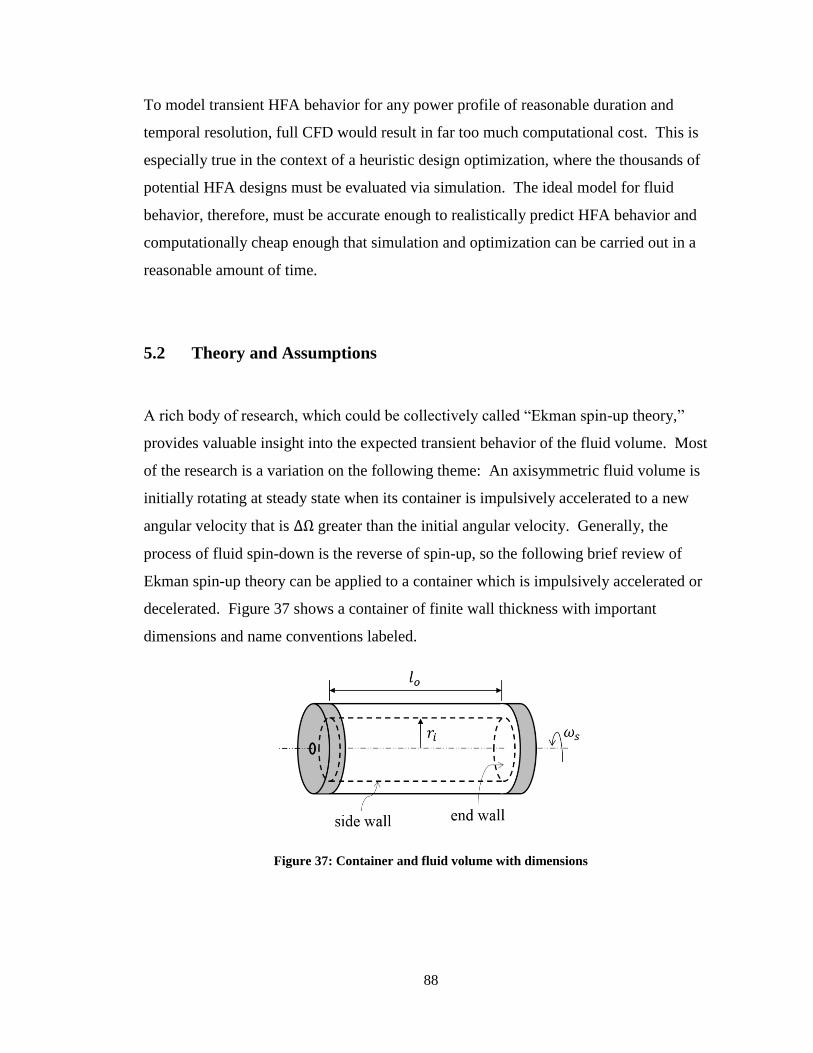
88

To model transient HFA behavior for any power profile of reasonable duration and

temporal resolution, full CFD would result in far too much computational cost. This is

especially true in the context of a heuristic design optimization, where the thousands of

potential HFA designs must be evaluated via simulation. The ideal model for fluid

behavior, therefore, must be accurate enough to realistically predict HFA behavior and

computationally cheap enough that simulation and optimization can be carried out in a

reasonable amount of time.

5.2 Theory and Assumptions

A rich body of research, which could be collectively called “Ekman spin-up theory,”

provides valuable insight into the expected transient behavior of the fluid volume. Most

of the research is a variation on the following theme: An axisymmetric fluid volume is

initially rotating at steady state when its container is impulsively accelerated to a new

angular velocity that is ΔΩ greater than the initial angular velocity. Generally, the

process of fluid spin-down is the reverse of spin-up, so the following brief review of

Ekman spin-up theory can be applied to a container which is impulsively accelerated or

decelerated. Figure 37 shows a container of finite wall thickness with important

dimensions and name conventions labeled.

Figure 37: Container and fluid volume with dimensions

89

Note that the axle is omitted from the present study on fluid behavior. Review of the

Ekman spin-up literature suggests that the fluid behavior is fundamentally the same,

regardless of whether the axle is present. The parameter 𝜔𝑠 refers to the container

angular velocity, where the subscript “𝑠” emphasizes that the container is composed of

solid components.

In the limiting case of an infinitely long (𝑙𝑜 = ∞) cylindrical fluid volume, any departure

from fluid rigid body rotation manifests itself as a one-dimensional flow relative to the

container. In this special case, all fluid velocity remains azimuthal (although its

magnitude varies with radial location), and transport of momentum within the fluid is

accomplished purely through viscous diffusion. However, for any reasonable set of

geometric dimensions, the HFA aspect ratio (𝑙𝑜/𝑟𝑖) is far too low for infinite length to be

a suitable approximation [65].

Instead, it turns out that the relative flow during transience is quite three-dimensional

(though still axisymmetric), with the end walls playing an extremely important role [66].

Due to the no-slip condition, an impulsive increase in the container angular velocity

results in a thin layer of fluid at each wall that rotates faster than the core flow. These

thin layers of fluid are subject, then, to a centrifugal field that overcomes the prevailing

pressure gradient (the pressure gradient imposed by the rotation of the core flow).

Consequently, fluid at the end walls is accelerated radially outward in what has become

known as an Ekman boundary layer. To satisfy continuity, the radial outflow is

accompanied by an axial inflow to the Ekman layer along the longitudinal axis of the

cylinder. Fluid leaving the Ekman layer at the outer radius is turned and travels axially

within the sidewall boundary layer. Near the meridian, the flow is turned again, such that

it travels radially inward to replace the axial inflow to the Ekman layer.

The radial inflow at the meridian can be envisioned as fluid rings which approximately

conserve angular momentum; as they travel inward, their angular velocity increases,

effectively spinning up the fluid. It is clear, then, that the dominant mechanism for fluid

spin-up is advective, not viscous. As a result, spin-up is accomplished much faster than it

would be is viscosity were the dominant mechanism. Specifically, spin-up is complete in

a time on the order of [66]

90

𝑡𝐸 =

𝑙𝑜

√𝜈𝑜Ω (124)

where 𝜈𝑜 is the kinematic viscosity of the fluid and Ω is a characteristic angular velocity.

Generally, Ω is chosen as larger of the initial and final angular velocities that define the

impulsive spin-up event. Note that the use of upper-case omegas in this chapter is

reserved for constants which describe a spin-up event, while lower-case omegas refer to

an instantaneous and time-varying angular velocities.

To contextualize the Ekman time constant, 𝑡𝐸, consider a cylindrical container of roughly

1 m length and aspect ratio 𝑙𝑜/𝑟𝑖 = 𝑂(1). The container is filled with hydraulic oil

(kinematic viscosity of 46 cSt) initially at steady state and is impulsively accelerated

from its original speed to 523.6 rad/s (5000 RPM). Equation 124 predicts (and

experiments have confirmed [66]) that spin-up is 95% complete in a time 𝑂(10 𝑠). If the

end wall Ekman effects were not present and momentum exchange was accomplished

purely via viscous diffusion, spin-up would be accomplished in a time scale 𝑙𝑜2/𝜈𝑜. This

turns out to be 𝑂(1000 𝑠) – two orders of magnitude higher than the advective spin-up

time.

Though conceptually useful, the theory developed in Ekman spin-up literature is

insufficient to actually model transient HFA behavior. Scenarios studied in the literature

analyze discrete spin-up events with well-defined initial and final conditions of steady

state rotation at specified angular velocities. The present situation is quite different, in

that an arbitrary power profile (as opposed to an angular velocity step change) is the

simulation input, and steady state rotation is not necessarily ever reached. To the

author’s knowledge, none of the literature treats the energy, which must include viscous

dissipation, required to accomplish a spin-up event, and none attempts to the model fluid

behavior that results from an arbitrary power profile.

Despite the infeasibility of direct application to a simulation, the Ekman spin-up theory

will be used to justify a key modeling assumption – and several extensions thereof – for

the development of the HFA fluid model. At all times, the fluid volume will be presumed

to act approximately as a rigid body spinning at angular velocity 𝜔𝑓. The difference

between the fluid angular velocity and its container is

91

Δ𝜔 = 𝜔𝑠 − 𝜔𝑓 (125)

At steady state, Δ𝜔 = 0, but during transience, Δ𝜔 ≠ 0. The proceeding arguments

provide justification for the fluid rigid body assumption, which may at first seem

contradictory to the preceding description of the three-dimensional flow phenomena and

to the arguments in Section 5.1.

Benton [67] provides the following rough approximations for the absolute radial,

azimuthal, and axial components of velocity in the core of the fluid. The equations are

valid for the case of an impulsive change in angular velocity of the container, from an

initial state of rigid-body rotation.

𝑢𝑟 ≅1

2𝑟ΔΩ√

𝜈𝑜𝑙𝑜2Ω

(126)

𝑢𝜃 ≅ 𝑟(Ω − ΔΩ) + 𝑟ΔΩ [1 − exp(−

√𝜈𝑜Ω𝑡

𝑙𝑜)] (127)

𝑢𝑧 ≅

ΔΩ

Ω√𝜈𝑜Ω (128)

In these equations, 𝑟 and 𝑡 are radial location and time, respectively. It is clear from

Eqns. 126 through 128 that, for any appreciable angular velocity and fluid viscosity, the

azimuthal component of fluid velocity is much greater than the radial and axial

components, which arise only due to Ekman circulation. The absolute kinetic energy in

the fluid consequently manifests itself primarily in the azimuthal flow component.

Therefore, although they are essential to the advective nature of fluid spin-up, the radial

and axial components of fluid velocity will be henceforth neglected in quantifying the

instantaneous amount of kinetic energy stored in the fluid.

Equation 127 offers two important points. First, azimuthal velocity is linearly dependent

on radial location and is independent of axial and tangential location, which is the

definition of rigid body rotation. Therefore, Benton’s azimuthal velocity equation serves

as the primary justification for the “fluid rigid body assumption,” the approximation that

the fluid volume spins roughly as a rigid body at an angular velocity 𝜔𝑓, even during

transient events.

92

The same equation also leads to the first extension of the fluid rigid body assumption:

The fluid angular velocity exhibits a first-order time response to a change, impulsive or

otherwise, in container angular velocity. In the case of Benton’s equation, the change in

container angular velocity is impulsive. To make it applicable to a simulation, several

modifications to Eqn. 127 must be introduced. Specifically, the linear velocity

distribution is converted to a fluid angular velocity, the constant ΔΩ is replaced by the

variable 𝛥𝜔 (defined by Eqn. 125), and the Ekman time constant (defined by Eqn. 124) is

replaced by a dynamic time constant, 𝜏𝑑.

𝜔𝑓𝑛+1 = 𝜔𝑓

𝑛 + Δ𝜔𝑛[1 − exp(−Δ𝑡/𝜏𝑑𝑛)] (129)

The qualifier “dynamic” for 𝜏𝑑 is used to reflect the fact that, if Eqn. 129 is applied to

each time step in a simulation, it is not expected that the Ekman time constant should

provide an appropriate estimate of fluid response (indeed, the constant Ω does not exist

for an arbitrary angular velocity profile). Instead, the degree to which the fluid “catches

up” to its container during a time step is expected to depend on various parameters that

describe the state of the HFA.

Wiedman [68] discusses the scenario where the container spins up at a constant finite

(non-impulsive) rate of acceleration. While he does not provide a time constant, he

suggests that the response of the fluid depends on the parameters in Eqn. 124, as well as

the rate of acceleration of the container, 𝛼𝑠. Because the duty cycle to be used in the

present research is arbitrary, the theory presented by neither Benton nor Weidman is

directly applicable.

The second important extension of the fluid rigid body assumption is that the pressure at

the center is indicative of the kinetic energy contained in the fluid volume. For any flow,

the kinetic energy contained in the fluid is equal to the volume integral of the specific

kinetic energy. For a constant-density fluid in rigid body rotation, with negligible radial

and axial velocity components, this becomes

𝐸𝑘,𝑓 = ∫1

2𝜌𝑜𝑢𝜃

2

𝑉

𝑑𝑉 = 𝜌𝜋𝑙𝑜 ∫ 𝑟2𝜔𝑓2

𝑟𝑖

𝑟=0

𝑟𝑑𝑟 (130)

93

Evaluation of the integral in Eqn. 130, unsurprisingly, yields an expression for kinetic

energy that is identical to that for a solid body.

𝐸𝑘,𝑓 =

1

4𝜌𝑜𝜋𝑙𝑜𝑟𝑖

4𝜔𝑓2 =

1

2𝐼𝑓𝜔𝑓

2 (131)

Since constant rigid body fluid rotation is assumed, Eqn. 25 (system pressure as a

function of pneumatic pressure and angular velocity) with 𝜔 = 𝜔𝑓 should hold, even

during transients. Rearranging, this equation yields Eqn. 132, which can be inserted into

Eqn. 131 to produce Eqn. 133, an expression for kinetic energy as a function of inlet

pressure.

𝜔𝑓 = [

4

𝜌𝑜𝑟𝑖2 (𝑃𝑝 − 𝑃𝑠)]

1/2

(132)

𝐸𝑘,𝑓 = 𝜋𝑙𝑜𝑟𝑖2(𝑃𝑝 − 𝑃𝑠) (133)

Thus, fluid angular velocity and the amount of kinetic energy stored in the fluid volume

can be inferred from the pressure, 𝑃𝑠, at the inlet of the HFA.

The final extension of the fluid rigid body assumption relates to regions of viscous

dissipation. It can be assumed that viscous effects are essentially confined to the

boundary layers [67, 69]. Besides lending credibility to the rigid fluid body model by

implying that velocity gradients in the core are quite small, this notion helps in

identifying parameters that are important to viscous dissipation rate. The picture of spin-

up developed so far illustrates a viscous flow scenario similar to cylindrical Couette flow

where the fluid and solid volumes are, respectively, the inner and outer cylinders, and the

boundary layers mate the azimuthal velocities of each. Whereas in canonical Couette

flow there is only a cylindrical viscous flow, in the present situation there is also a

boundary layer at each end wall (the Ekman layers). Both the Ekman and side wall

boundary layers scale as

𝛿~√

𝜈𝑜Ω

(134)

and are roughly constant throughout the spin-up process [67].

94

5.3 Modeling Approach

To take into account viscous losses and fluid inertial behavior, simulation of HFA

response to a power profile is more complicated than simply applying Newton’s second

law. Instead, the kinetic energy equation below is used, where 𝑊𝑡̇ is tractive power

(allocated completely to the kinetic domain for the purposes of the present chapter), the

known input to the simulation.

𝑊𝑡̇ =

𝑑

𝑑𝑡𝐸𝑘,𝑠 +

𝑑

𝑑𝑡𝐸𝑘,𝑓 + �̇�𝑣 (135)

Notice that tractive power (positive when charging the HFA) is distributed between three

terms: One which changes the kinetic energy of the solid components, 𝐸𝑘,𝑠; one which

changes the kinetic energy of the fluid components, 𝐸𝑘,𝑓; and one which represents

viscous dissipation rate, �̇�𝑣. The latter, which is always positive, acts to decrease the

amount of kinetic energy gain during charging and increase the kinetic energy loss during

discharging.

Evaluating the derivatives in Eqn. 135 and using the fluid rigid body assumption leads to

a new form of the kinetic energy equation:

𝑊𝑡̇ = 𝐼𝑠𝛼𝑠𝜔𝑠 + 𝐼𝑓𝛼𝑓𝜔𝑓 + �̇�𝑣 (136)

To highlight the expected nature of the fluid response, it is convenient to express 𝛼𝑓 as

the average acceleration over a time step for a first order response.

𝛼𝑓 =

Δ𝜔

Δ𝑡(1 − exp (

𝛥𝑡

𝜏𝑑)) (137)

Equations 136 and 137 represent a system of two equations and four unknowns (𝛼𝑠, 𝛼𝑓,

�̇�𝑣 , and 𝜏𝑑). To render the simulation solvable, two empirical correlations must be

developed, one for the dynamic time constant and one for the viscous dissipation rate.

Algorithmically, the simulation is carried out by sequentially solving the following

equations, which are written in finite difference form.

95

𝛼𝑓𝑛+1 =

Δ𝜔𝑛

Δ𝑡(1 − exp(

𝛥𝑡

𝜏𝑑𝑛)) (138)

𝜔𝑓𝑛+1 = 𝜔𝑓

𝑛 + 𝛼𝑓𝑛+1Δ𝑡 (139)

𝛼𝑠𝑛+1 =

1

𝐼𝑠𝜔𝑠𝑛 (�̇�𝑡

𝑛+1 − 𝐼𝑓𝜔𝑓𝑛+1𝛼𝑓

𝑛+1 − �̇�𝑣𝑛) (140)

𝜔𝑠𝑛+1 = 𝜔𝑠

𝑛 + 𝛼𝑠𝑛+1Δ𝑡 (141)

�̇�𝑣𝑛+1 = 𝑓1(… ) (142)

𝜏𝑑𝑛+1 = 𝑓2(… ) (143)

Note that Eqn. 140 is simply the kinetic energy equation (Eqn. 136) rearranged to solve

for the container angular velocity. Equations 142 and 143 are generic representations of

the two desired empirical correlations, where the ellipses represent some combination of

known parameters from time step 𝑛.

The first step in developing the actual predictive equations represented by Eqns. 142 and

143 is to perform dimensional analysis. It is reasonable to assume that viscous

dissipation rate during a fluid transient will be affected by fluid properties, container

geometry, the boundary layer thickness, and the difference between the fluid and

container angular velocities. Given these assumptions, the dimensional analysis problem

is posed as

�̇�𝑣𝑛 = 𝑓1(𝜌𝑜 , 𝜇𝑜 , 𝑙𝑜 , 𝑟𝑖,Δ𝜔,𝜔𝑠) (144)

This yields four dimensionless groups, each of which has been oriented (i.e. selection of

the numerator versus the denominator) to reflect its expected impact on viscous

dissipation rate.

�̇�𝑣

𝜇𝑜𝑟𝑖3𝛥𝜔2

= 𝜙1 (√𝜌𝑜𝜔𝑠𝑙𝑜2

𝜇𝑜,𝑙𝑜𝑟𝑖,𝛥𝜔

𝜔𝑠) = 𝜙1(𝑙𝑜/𝛿, 𝐴𝑅, 𝜖𝑑) (145)

Scaling parameters in the dependent dimensionless group are chosen such that viscous

dissipation rate goes to zero as Δ𝜔 goes to zero, a condition that is physically expected.

Returning to the expression for boundary layer thickness (Eqn. 134), the first independent

group in Eqn. 145 can be considered the inverse of a dimensionless boundary layer

thickness (It could also be considered the square root of a Reynold’s number). The

96

second independent term is a container aspect ratio, defined to be consistent with the

notion that spin-up in longer cylinders tends to be dominated by viscous, not advective,

effects. The final independent dimensionless group is deemed the dynamic Rossby

number (a transient counterpart to the Rossy number, ΔΩ/Ω, used in spin-up literature to

describe an impulsive acceleration event [66]) Again, this group is oriented such that its

value goes to zero when there is no relative velocity between the fluid and its container.

In consideration of the discussion of spin-up literature, it is expected that angular velocity

and acceleration of the container, as well as fluid viscosity and container length, are

important parameters in predicting the dynamic time constant. The dimensional analysis

problem is therefore posed as

𝜏𝑑 = 𝑓2(𝜈𝑜 , 𝑙𝑜 , 𝜔𝑠, 𝛼𝑠) (146)

This yields the following dimensionless relationship.

1

𝜏𝑑𝜔𝑠= 𝜙2 (

𝑙𝑜4𝛼𝑠𝜈𝑜2

,𝛼𝑠𝜔𝑠2) (147)

To avoid a divide-by-zero error for 𝛼𝑠 → 0, container acceleration must be placed in the

numerator of the independent groups. Then, the dynamic time constant is placed in the

denominator of the dependent group to reflect the experimental observation that 𝜏𝑑

decreases as 𝛼𝑠 increases.

Equations 145 and 147 indicate the dimensionless groups that are expected to be

important in predicting the viscous dissipation rate and dynamic time constant,

respectively. Now, experiments can be used to obtain actual mathematical expressions

that describe the relationships between these groups.

5.4 Experimental Approach

The experimental apparatus must apply a transient power trace to a rotating fluid volume.

During an experiment, it is necessary to measure several physical quantities is order to

calculate the various parameters in Eqns. 145 and 147. Then, a curve-fitting algorithm

97

can be used to derive an actual mathematical relationship between the dimensionless

groups. Figure 38 illustrates the experimental setup.

Figure 38: Experimental Setup with Instrumentation

A rotating cylinder filled with oil is driven by a hydraulic motor. Flow rate through the

motor is metered using a proportioning flow control valve in a feedback control loop. In

this way, the angular velocity of the rotating cylinder can be accurately-controlled. A

rotary torque sensor and shaft encoder facilitate torque and speed measurements, and a

rotary union allows for an internal pressure tap at the center of an end cap. Because the

cylinder is not charged, the pneumatic pressure is effectively zero at all times. The

system pressure equation (Eqn. 25) indicates that gage pressure at the center should then

be negative for any nonzero rotational speed. Tables 11 and 12 provide relevant

specifications for the experimental setup.

Table 11: General Specifications for the Experimental Setup

Oil length, 𝒍𝒐 [𝒄𝒎] 30

Oil radius, 𝒓𝒊 [𝒄𝒎] 5.7

Oil density, 𝝆𝒐 [𝒌𝒈/𝒎𝟑] 879

Oil kinematic viscosity, 𝝂𝒐 [𝒄𝑺𝒕] 46

Maximum speed [𝑹𝑷𝑴] 1100

Sampling frequency [𝑯𝒛] 1000

98

Table 12: Specifications of the Equipment Used for the Experimental Setup

Hydraulic pump-motor

Manufacturer Parker

Model number MGG20020

Displacement [𝒄𝒄/𝒓𝒆𝒗] 7.4

Rated pressure (continuous) [𝒃𝒂𝒓] 138.0

Rated pressure (intermittent) [𝒃𝒂𝒓] 172.5

Rated flow per 1000 RPM [𝒍𝒑𝒎] 7.4

Proportional flow control valve

Manufacturer Eaton

Model number EPFB-10

Rated pressure (continuous) [𝒃𝒂𝒓] 350

Rated flow [𝒍𝒑𝒎] 30.3

Power supply 24 VDC, 1.1 amps

Valve cavity #C1030

Torque sensor

Manufacturer Futek

Model number TRS300

Item number FSH01988

Torque capacity [𝑵𝒎] 20

Maximum speed [𝑹𝑷𝑴] 3000

Shaft encoder

Manufacturer US Digital

Model ETACH2

Max. input frequency [𝑯𝒛] 12.7 MHz (adjustable)

Vacuum gauge

Manufacturer Honeywell

Part number 40PC015V2A

Pressure range [𝒑𝒔𝒊] 0 to -15

99

Note that angular velocity is the prescribed physical quantity for any given experiment,

and therefore the applied power is, in a sense, incidental. For the purposes of

characterizing viscous dissipation rate and dynamic time constant, this is perfectly

acceptable, as the actual shape of the power profile is non-critical; the important point is

that the applied power can be extracted from the measured data.

To confirm repeatability of measurements, the prescribed angular velocity traces are non-

arbitrary. Instead, they resemble near-impulsive acceleration events, and to maximize the

signal to noise ratio of the torque sensor, the angular velocity traces are rather aggressive.

As shown in the complete results in Appendix C, such events tend to utilize between 10%

and 25% of the range of the torque sensor. Figure 39 shows an example angular velocity

trace used for model development, along with its equivalent ideal (step change) trace.

Though not fully shown in the plot, container angular velocity is held constant before and

after the transient for a time deemed sufficient to guarantee steady state (at least six

Ekman time constants, as defined by Eqn. 124).

Figure 39: Example of an Attempted Step Change from 200 RPM to 1000 RPM, Desired and

Achieved

The extraction of the applied power profile for an experiment and the subsequent

calculations of other important parameters are carried out as follows. The torque on the

experimental setup due to bearing friction and aerodynamic drag has been characterized

as a function of angular velocity. For any experiment, this is subtracted from the

100

measured torque, 𝑇𝑚, the result of which is multiplied by angular velocity to calculate the

applied power profile,

𝑊𝑡̇ = (𝑇𝑚 − 𝑇𝑏 − 𝑇𝑤)𝜔𝑠 = 𝑇𝜔𝑠 (148)

The measured system pressure is used to calculate fluid angular velocity using Eqn. 132.

Doing so relies on the reasonable assumption that the pressure gradient across the Ekman

boundary layer is negligible [70].

Due to the high sampling frequency, even a small amount of noise in the fluid and solid

angular velocity profiles makes it difficult to obtain coherent traces of their time

derivatives. To cope with this issue, the angular velocity traces are filtered and then

smoothed with cubic splines. The corresponding angular acceleration traces can then be

obtained by using the analytical derivatives of the splines. Figure 40 illustrates the utility

of this strategy with an example profile of fluid angular acceleration. The lighter curve

has been produced by using a low-pass filter on angular velocity data and then

numerically differentiating the result. The darker line has been produced by spline-fitting

the filtered angular velocity data and analytically differentiating the result. The cutoff

frequency of the filter is 30 Hz and the spline has been constructed using a rate of 5.8

knots per second of data. To illustrate the accuracy of the fluid angular acceleration

curve produced by the spline strategy, the plot also includes a dotted curve showing the

solid angular acceleration, which should be qualitatively similar.

The importance of the spline strategy is made clear upon examination of Fig. 40, where

the curve produced from the filtered but un-splined data is noisy to the point of

uselessness. In the course of post-processing, the number of knots used in the spline is

manually-adjusted for each dataset, such that a smooth fit to the filtered angular velocity

data is produced without the spline actually following the noise of the signal. For all of

the present datasets, this can be accomplished using a rate of 20 knots per second or less.

101

Figure 40: Example of Spline-fitting Strategy to Produce Smooth Acceleration

Having calculated the angular acceleration traces, distribution of the applied power can

be inferred. The power to the solid components (the container) can be calculated as the

rate of change of its kinetic energy,

�̇�𝑠 = 𝐼𝑠𝛼𝑠𝜔𝑠 (149)

and the power to the fluid components is calculated as the difference between the applied

power (Eqn. 148) and the power going to the solid components (Eqn. 149):

�̇�𝑓 = 𝑊𝑡̇ − �̇�𝑠 (150)

The power to the fluid components can be further split into that which contributes to

changing the kinetic energy of the fluid volume and that which is dissipated by viscosity.

Thus, viscous dissipation rate is

�̇�𝑣 = �̇�𝑓 − 𝐼𝑓𝛼𝑓𝜔𝑓 (151)

Finally, the dynamic time constant is calculated as

𝜏𝑑 = −

Δ𝑡

ln (1 −𝛼𝑓𝛥𝑡𝛥𝜔 )

(152)

Hence all quantities in Eqns. 145 and 147 have been either measured directly or

calculated based on measurements, such that values for the actual dimensionless groups

102

can be calculated. It is now possible to begin tying together the theoretical and

experimental approaches.

5.5 Model Development

For all experimental datasets, the signal-to-noise ratio of the torque sensor is most

favorable during the transient section, when a significant portion of the sensor capacity is

utilized. For this reason, only the data in the transient section is used in generating

correlations for the fluid model.

Because the experimental setup has a fixed geometry, the second dimensionless group in

the viscous dissipation correlation is constant for all experiments. Therefore, the

correlation space is three-dimensional for both the viscous dissipation rate and the

dynamic time constant. In choosing the form of an equation for the correlations,

however, three-dimensional scatter plots offer fairly little insight. Lacking any

justification based on fluid mechanics, polynomial fits are chosen in anticipation of them

being the most versatile. Equation 153 illustrates the form of a correlation, where 𝜋1 is

the dependent dimensionless group, the Π𝑗’s are the independent dimensionless groups,

𝑘𝑜 is a constant, and 𝑘𝑗𝑛 is the coefficient for term which raises the 𝑗𝑡ℎ independent group

to the 𝑛𝑡ℎ power.

Π1 = 𝑘𝑜 +∑∑𝑘𝑗𝑛Π𝑗𝑛

𝑛

1

𝑗

2

(153)

For both correlations, 𝑗 = 2. The viscous dissipation data is found to fit quite well to a

third-order polynomial and the dynamic time constant data to a second-order polynomial.

The optimal coefficients for each correlation (7 coefficients for the viscous dissipation

rate and 5 for the time constant) are found by using a genetic algorithm that minimizes

the sum of squared errors.

Eleven experiments have been run with the desired angular velocity trace shown in Fig.

39 (200 RPM to 1000 RPM, near-impulsive), and the complete data for each are provided

103

in Appendix C. Each experiment yields a dataset from which both a viscous dissipation

and a dynamic time constant correlation can be developed. The two correlations from

each dataset can and should be assessed completely independently from one another.

That is, the time constant correlation from experiment #1 is no more “related” to the

viscous dissipation correlation from experiment #1 than it is to the viscous dissipation

correlation from experiment #2. Therefore, the experiments yield twenty-two

independent correlations, eleven candidates for the best viscous dissipation correlation

and eleven candidates for the best dynamic time constant correlation.

The validity of each of the correlations is assessed by applying it to each of the power

profiles from the other ten experimental datasets. In other words, a correlation developed

by curve-fitting data from experiment #1 can be tested by running a simulation where the

power profile from experiment #2 is the input, and then comparing the resultant

simulated data (viscous dissipation rate, fluid and solid angular velocity, etc.) to the

measured data from experiment #2. In this way, twenty-two different correlations

(eleven each for the two desired parameters) are evaluated via 220 simulations.

Over the course of a simulation, the accuracy of the dynamic time constant correlation

affects the indicated accuracy of the viscous dissipation correlation, and vice versa. For

example, should the dynamic time constant correlation tend to under-predict the correct

(measured) value, the viscous dissipation rate will consequently be under-predicted. This

is intuitive, as a lower-than-realistic Δ𝜔 should result in lower-than-realistic viscous

dissipation. For this reason, while the viscous dissipation correlations are being

evaluated and compared, the dynamic time constant is intentionally forced to its

measured value. Then, once the best viscous dissipation correlation has been identified,

it is permanently embedded in the simulation code, such that its effects are included

during the evaluation and comparison of the candidate dynamic time constant

correlations.

Quantitatively, the performance of a correlation is judged by how well it predicts

container and fluid angular velocities. To constitute such a judgment, the coefficient of

determination, defined as

104

𝑅2 =

𝑅𝑠2 + 𝑅𝑓

2

2 (154)

is used, where

𝑅𝑖2 = 1 −

∑(𝜔𝑖,𝑚𝑒𝑎𝑠𝑢𝑟𝑒𝑑 − 𝜔𝑖,𝑝𝑟𝑒𝑑𝑖𝑐𝑡𝑒𝑑)2

∑𝜔𝑖,𝑚𝑒𝑎𝑠𝑢𝑟𝑒𝑑2 (155)

To provide more qualitative insight into how a given correlation performs, two different

coefficients of determination can be calculated:

𝑅952 , which includes the highly transient region between the initial acceleration

and the time at which the measured fluid angular velocity has reached 95% of its

steady state value, and

𝑅992 , which includes the region between the initial acceleration and the time at

which the measured fluid angular velocity has reached 99% of its steady state

value. This generally includes a much larger amount of near-steady state

behavior

Any given correlation might perform quite differently in the highly transient section

compared to the near-steady state section; examination of the two different coefficients of

determination defined above provides insight into this difference.

Table 13 shows the values of 𝑅952 , 𝑅99

2 , and 𝑅𝑜𝑣𝑒𝑟𝑎𝑙𝑙2 = (𝑅95

2 + 𝑅992 )/2, for each of the

eleven candidate viscous dissipation correlations. All of these 𝑅2 values encompass data

from all ten simulations for a given correlation, such that they represent its average

performance. The correlations are ranked by 𝑅𝑜𝑣𝑒𝑟𝑎𝑙𝑙2 .

105

Table 13: Ranked Performance of the Viscous Dissipation Rate Correlations, Based on Coefficient of

Determination

Corr. # Rank 𝑹𝒐𝒗𝒆𝒓𝒂𝒍𝒍𝟐 𝑹𝟗𝟓

𝟐 𝑹𝟗𝟗𝟐

7 1 0.99845 0.998825 0.998067

9 2 0.99843 0.999039 0.997830

3 3 0.99816 0.998836 0.997490

4 4 0.99805 0.998773 0.997335

1 5 0.99795 0.999171 0.996733

6 6 0.99794 0.998850 0.997036

8 7 0.99781 0.998125 0.997489

2 8 0.99685 0.998603 0.995093

11 9 0.99675 0.998599 0.994908

5 10 0.99646 0.998460 0.994452

10 11 0.99624 0.998629 0.993850

Average 0.99755 0.998719 0.996389

Standard Dev. 0.00081 0.000284 0.001511

On average, a viscous dissipation correlation predicts the container and fluid angular

velocities with at 𝑅𝑜𝑣𝑒𝑟𝑎𝑙𝑙2 = 0.998. Quantitatively, there is relatively little difference in

how well the correlations behave through 95% of steady state. Including data through

99% causes in increase in total squared error for all correlations and reveals more

variation amongst them, increasing standard deviation by an order of magnitude. In other

words, there is a wider range of performance amongst the correlations for steady state,

but each performs worse at steady state than it does during transience.

Because it produces the highest value of 𝑅𝑜𝑣𝑒𝑟𝑎𝑙𝑙2 , viscous dissipation correlation #7 is

selected for use in the fluid model. As indicated in Table 13, this correlation performs

better than all but two in transience, and better than any other when data through 99% of

steady state is included. The full expression for the selected viscous dissipation

correlation is:

106

�̇�𝑣

𝜇𝑜𝑟3𝛥𝜔2= 4.16(103) + 6.69√

𝜌𝑜𝜔𝑠𝑙𝑜2

𝜇𝑜…

−1.77(10−2) [√𝜌𝑜𝜔𝑠𝑙𝑜2

𝜇𝑜]

2

+ 1.95(10−5) [√𝜌𝑜𝜔𝑠𝑙𝑜2

𝜇𝑜]

3

…

−2.18(104)𝛥𝜔

𝜔𝑠+ 1.38(105) [

𝛥𝜔

𝜔𝑠]3

(156)

Notice that the first independent group contributes a full cubic polynomial to the

correlation, while only a linear and a cubic term are contributed by the second

independent group (the quadratic coefficient was forced to zero by the curve-fitting

algorithm). Figure 41 illustrates the relative contribution of each independent group for

the transient portion of an example simulation. For ease of plotting, the constant 𝑘𝑜 has

been grouped with the terms contributed by the second independent group.

Figure 41: Example Dataset Showing the Relative Contributions of Independent Groups in the

Viscous Dissipation Correlation

Figure 41 expresses what is difficult to discern from simply examining Eqn. 156. Most

of the transient behavior of the dependent group, �̇�𝑣/𝜇𝑜𝑟𝑖3Δ𝜔2, is contributed by the

60 62 64 66 68 70 72500

1000

1500

2000

2500

3000

3500

4000

4500

5000

time (s)

dim

ensio

nle

ss v

alu

e

107

second independent group, Δ𝜔/𝜔𝑠, while the first independent group, √𝜌𝑜𝜔𝑠𝑙𝑜2/𝜇𝑜, acts

somewhat like a constant offset. This observation suggests that the fluid angular velocity

relative to its container is more important than the estimated boundary layer thickness in

predicting viscous dissipation rate.

Having identified the best viscous dissipation rate correlation, it can now be embedded

into the simulation in order to assess the performance of the eleven candidate dynamic

time constant correlations. During evaluation, three are deemed invalid due to observed

instability during one or more simulations. The remaining time constant correlations are

ranked in Table 14 by their overall combined performance with the selected viscous

dissipation correlation.

Table 14: Ranked Performance of the Dynamic Time Constant Correlations, Based on Coefficient of

Determination

Corr. # Rank 𝑹𝒐𝒗𝒆𝒓𝒂𝒍𝒍𝟐 𝑹𝟗𝟓

𝟐 𝑹𝟗𝟗𝟐

8 1 0.99549 0.99726 0.99371

6 2 0.99513 0.99749 0.99276

7 3 0.99444 0.99614 0.99274

11 4 0.99371 0.99697 0.99045

5 5 0.99286 0.99692 0.98879

9 6 0.99247 0.99670 0.98823

1 7 0.99151 0.99585 0.98718

10 8 0.64704 0.64414 0.64995

Average 0.95033 0.95268 0.94798

Standard Dev. 0.12257 0.12467 0.12044

As expected, the average 𝑅𝑜𝑣𝑒𝑟𝑎𝑙𝑙2 for the simulations presented in Table 14 is lower than

those in Table 13, where, instead of using a correlation, dynamic time constant was

forced to the correct value. Still, the quality of simulations is quite high, especially in the

transient 95% region.

108

Again using the criterion of highest 𝑅𝑜𝑣𝑒𝑟𝑎𝑙𝑙2 , the dynamic time constant correlation #8 is

chosen for use in the fluid model. Its full expression is:

1

𝜏𝑑𝜔𝑠= 3.90(10−3) − 3.76(10−19) [

𝑙𝑜4𝛼𝑠𝜈𝑜2

]

2

+ 2.54𝛼𝑠𝜔𝑠2

+ 4.07 [𝛼𝑠𝜔𝑠2]2

(157)

While the dependent quantity 1/𝜏𝑑𝜔𝑠 exhibits both linear and quadratic dependence on

the second independent group, the linear term from the first independent group was

eliminated by the curve-fitting algorithm. The exact value of the small constant offset

turns out not to matter, as it contributes a negligible amount to the value of 1/𝜏𝑑𝜔𝑠. The

offset exists only as a numerical barrier to calculating an infinite dynamic time constant

when acceleration rate goes to zero. Figure 42 shows an excerpt from a simulation that

illustrates the relative importance of the two independent groups in the dynamic time

constant correlation.

Figure 42: Example Dataset Showing the Relative Contributions of Terms in the Dynamic Time

Constant Correlation

As was the case for the viscous dissipation correlation, the relative contribution from the

two independent variables is rather lopsided. The dependent variable response is dictated

60 60.2 60.4 60.6 60.8 61 61.2 61.4 61.6 61.8 62-0.1

0

0.1

0.2

0.3

0.4

0.5

0.6

time (s)

dim

ensio

nle

ss v

alu

e

109

mostly by the behavior of the term 𝛼𝑠/𝜔𝑠2 and corrected only slightly by the 𝑙𝑜

4𝛼𝑠/𝜈𝑜

term.

It is worth noting that, as steady state is approached, error in the predicted dynamic time

constant becomes simultaneously greater in value and less important in effect. The

former is true because the time constant is inversely proportional to the container

acceleration and therefore more sensitive to error as acceleration goes to zero. The latter

is true because, as steady state is approached, Δ𝜔 shrinks, and therefore any error in the

predicted time constant is multiplied by a smaller value in the calculation of the fluid

velocity for the subsequent time step.

5.6 Model Validation

The predictive model, whose development has been detailed in the preceding sections,

can be executed with only a few lines of code. To prove this, various simulations were

run using MATLAB® on a modest processor. Even without any attempt to maximize

computational efficiency, three minutes of physical time with one millisecond temporal

resolution can be simulated in approximately one second of computational time. In this

regard, the requirement that the model be computationally inexpensive has been

overwhelmingly achieved.

In addition the requirement of computational simplicity, the fluid model must realistically

predict HFA behavior. Before assessing the model performance in this regard, a certain

unanticipated nuance in the measured fluid behavior must be described. In experiments

with significant overshoot and rapid recovery of container angular velocity to the

command step signal, a negative measured time constant can be observed for a small

period of time. An example is illustrated in Fig. 43, where the fluid angular velocity can

be seen to follow a qualitatively similar profile as the container angular velocity, peaking

and beginning to decrease, even though Δ𝜔 never ceases to be positive.

110

Figure 43: Example of a Region with an Observed Negative Dynamic Time Constant

To the author’s knowledge, there is no physical explanation for the region of observed

negative time constant shown in Fig. 43; the fluid angular velocity should increase as

long as it remains below the container angular velocity. It is therefore postulated that,

during strong acceleration, flow phenomena in the Ekman boundary layer generate a

pressure gradient that causes the pressure sensor to read somewhat lower (more vacuum)

than the true value in the fluid core. This is translated via Eqn. 132 to a somewhat over-

predicted fluid angular velocity. A sudden deceleration of the container is accompanied

by a reversal in the aforementioned flow phenomena, the net result of which is to

generate a fluid angular velocity trace which exhibits some non-physical behavior.

It must be noted that characterizing a dynamic time constant is extremely useful,

regardless of how well the measured pressure actually indicates fluid angular velocity.

Regardless of whether it is valid to assume that no pressure gradient exists across the

Ekman layer, the pressure measured in the present experiments is, in fact, the pressure

that the hydraulic system would experience in an actual HFA application. The ability to

predict the transient system pressure behavior is essential in developing an effective

control strategy. The detrimental effect of the non-physical behavior shown in Fig. 43,

then, is to overestimate (in positive acceleration) the rate of change of fluid kinetic

energy, thereby introducing some error into the energy equation (Eqn. 136). For the

111

purposes of assessing model performance, the remainder of the discussion relies on the

assumption that the calculated fluid angular velocity is reasonably accurate.

As a general illustration of the performance of the model, Figures 44, 45 and 46 show

angular velocities, dynamic time constant, and viscous dissipation rate, respectively, for

the transient portion of an example simulation. The plots show simulated quantities and

their corresponding measured quantities. This example comes from a dataset that,

importantly, is not the same one that generated either of the correlations chosen for the

fluid model. For this example, 𝑅952 = 0.9998.


Acceleration from 200-1000 RPM

59 60 61 62 63 64 65 66 67 68 69 7020

40

60

80

100

120

time (s)

(

rad/s

)

solid, measured

solid, model-predicted

fluid, measured

fluid, model-predicted

112

Figure 45: Dynamic Time Constant, Measured Versus Simulated, Near-Impulsive Acceleration from

200-1000 RPM

Figure 46: Viscous Dissipation Rate, Measured Versus Simulated, Near-Impulsive Acceleration from

200-1000 RPM

Figure 44 shows that, qualitatively, the fluid model predicts container and fluid angular

velocities quite well for the transient section of an aggressive acceleration event. For the

first two seconds after the onset of acceleration, time constant and viscous dissipation rate

59 60 61 62 63 64 65 66 67 68 69 70-8

-6

-4

-2

0

2

4

6

8

10

time (s)

d (

s)

measured

model-predicted

59 60 61 62 63 64 65 66 67 68 69 70-10

-5

0

5

10

15

time (s)

_W

vl

(W)

measured

model-predicted

113

are very well-predicted, leading to near perfect agreement between measured and

simulated angular velocities. The first spike in container angular velocity is initially

handled well, but near 62 seconds, Fig. 45 shows that the time constant begins to be over-

predicted. This has the effect of predicting a Δ𝜔 that is slightly too large, which in turns

leads to an over-prediction of viscous dissipation, which can be seen in Fig. 46. When

steady state is nearly reached, the time constant begins to be under-predicted, such that

simulated fluid and solid angular velocities converge somewhat too early.

Though there is noticeable error in the predicted viscous dissipation rate, its integral is

very near that of the measured viscous dissipation rate. Therefore, the net dissipated

energy is predicted quite accurately, and the simulated angular velocities converge to the

correct value. Negative values of measured dissipation rate are non-physical and are

attributed to noise in the data. Figure 46 shows that the formulation of Eqn. 157 properly

avoids the prediction of any negative dissipation rate.

Recall that, to maximize the utilized range of the torque sensor, only experimental runs

with the relatively aggressive case of near-impulsive 200-1000 RPM have been used in

the development of the fluid model. The model performance is diminished to varying

extents when applied to other transient cases. Figure 47 shows measured and predicted

angular velocity traces for the smaller near-impulsive acceleration event of 200-600

RPM. For this transient section, 𝑅952 = 0.9979, slightly lower than the 200-1000 RPM

case. The same qualitative trends are observed for both cases. Time constant and

viscous dissipation rate are initially predicted quite well. The spike in container angular

velocity has a small detrimental effect on the latter, causing the simulated angular

velocities to reach steady state too soon. A slight over-prediction in net dissipated energy

causes the final simulated angular velocity to be a few radians per second lower than the

measured value. In full, the model proves to be fairly robust for the 200-600 RPM near-

impulsive case.

114



The model performance suffers much more when the initial angular velocity is different

than that which was used to produce the correlations. Figure 48 shows the case of near-

impulsive acceleration from 600-1000 RPM. In this case, 𝑅952 = 0.9874, which is

significantly lower than either of the previously presented cases. The model substantially

over-predicts the dynamic time constant from the beginning of the transient. While

predicted container angular velocity is initially quite accurate, the artificially large Δ𝜔

generates an erroneously high simulated rate of viscous diffusion. This drags the

predicted steady state angular velocity down to a value significantly below the correct

value.

89 90 91 92 93 94 95 96 97 98 99 10020

30

40

50

60

70

80

time (s)

(

rad/s

)

solid, measured


fluid, measured


115



As a final example of the versatility of the fluid model, it is useful to examine the case of

a non-impulsive acceleration. Figure 49 shows the predicted and measured angular

velocities for the case of a mild acceleration from 100-800 RPM over the course of about

12.5 seconds. Compared to the near-impulsive 200-1000 RPM example illustrated in

Figures 44 through 46, the average acceleration for this milder case is lower by a factor

of three, and the maximum observed rate of acceleration is lower by a factor of ten.

Qualitatively, the model performance for this transient section falls somewhere between

the two shorter, near-impulsive cases shown in Figures 47 and 48. Here, however, the

viscous dissipation rate is the more error-prone correlation. The measured viscous

dissipation rate is so close to zero that the model tends to over-predict it. The result of

this it under-predict both angular velocities, even though the time constant is reasonably

accurate.

60 61 62 63 64 65 66 67 68 69 7060

70

80

90

100

110

120

130

time (s)

(

rad/s

)

solid, measured


fluid, measured


116

Figure 49: Fluid and Container Angular Velocities, Measured Versus Simulated, Gradual


5.7 Closing Remarks about the Internal Fluid Modeling

The model developed in this chapter relies on the assumption that, under applied power,

the fluid volume accelerates roughly as a rigid body and lags behind its container in a

manner that can be modeled as a first-order time response. The simplicity of the model

allows it to simulate the transient HFA performance orders of magnitude more quickly

than would be possible if CFD were used. This makes it quite applicable to a highly-

resolved drive cycle simulation nested within a comprehensive design optimization.

By comparing simulations to measured data, the fluid model was shown to perform well

for transient sections of intense acceleration and large ΔΩ. To varying degrees, the

performance of the model was observed to decrease when applied to other types of

transients. For intense accelerations in general, the model predicts viscous dissipation

rate quite well. However, when the initial angular velocity is very far from that used to

60 62 64 66 68 70 72 74 76 78 800

10

20

30

40

50

60

70

80

90

time (s)

(

rad/s

)

solid, measured


fluid, measured


117

develop the correlation (200 RPM), prediction of the dynamic time constant is notably

hindered. Conversely, for cases where acceleration is milder, time constant is accurately

predicted, while viscous dissipation rate tends to be over-predicted. To improve the

robustness of the model, experimental data representing a wider variety of transients will

be used in future work.

During experimental data collection, pressure was measured at 𝑟 = 0 at the face of one of

the container end caps. There is some uncertainty as to how well this pressure

measurement indicates the true pressure in the fluid core. Future work will deal with this

uncertainty by either modifying the experimental apparatus to measure pressure away

from the end cap, or by attempting to characterize the pressure gradient across the

boundary layer that might arise from Ekman flow phenomena.

Finally, it is important to note that the model developed and assessed in this chapter is

specific to the experimental setup used to create it. Container aspect ratio, which was

included as an independent group in the dimensional analysis, was not varied in the

experiments, and was therefore not correlated. To make the model more reliable for use

in a design optimization, all relevant dimensionless groups must be correlated. Future

work will include the ability to vary the geometry of the container and/or the fluid

properties used in the experiments. Lacking a variable-geometry experimental apparatus

at the time writing, the fluid behavior model defined by Eqns. 156 and 157 is assumed to

be sufficient for the design optimization presented in Chapter 7. The fact that internal

viscous energy dissipation turns out to be very small compared to several other loss

mechanisms helps to justify this assumption.

118

6 Drive Cycle Simulation

The ability to accurately simulate the performance of the HFA by using computer models

is extremely valuable. To select an HFA design solution by optimizing a duty cycle-

dependent performance metric (e.g. efficiency, peak power), it is essential to embed a

performance simulation into the optimization algorithm. Duty cycle simulation can also

facilitate tradeoff studies on alternative control strategies and powertrain architectures.

This chapter details the development of tools that facilitate simulation of the HFA

operation and assessment of its performance. First, the selections of a particular duty

cycle and control strategy are justified. This is followed by a step-by-step description of

the calculation sequence that constitutes a simulation. The chapter concludes by

describing the calculations behind several important HFA performance metrics.

6.1 Road Loads and Vehicle Parameters

Section 2.1 defined the concept of specifying a particular HFA as a design solution (a set

of design variables), and Chapter 3 detailed the static calculations that can be performed

on such a design solution (e.g. selecting the remaining component dimensions,

calculating HFA mass). In addition to these specifications and calculations, a duty cycle

and a control strategy must be specified before carrying out a performance simulation.

The simulation tools developed in the present research facilitate easy exchange of

alternative duty cycles and control strategies. However, for various reasons, some

choices that pertain to performance simulation have become conventional over the course

of the research. These choices are detailed in this and the following sections.

A time-varying power profile, 𝑊𝑡̇ (𝑡), constitutes a duty cycle, which serves as the input

to a performance simulation of an energy storage system. In the case of simulating the

HFA performance, 𝑊𝑡̇ (𝑡) is the tractive power that was introduced in Section 2.5. While

this power profile can be specified directly, it is more conventional in road vehicle

performance modeling to calculate transient power from the combination of a time-

119

varying velocity profile and a set of specified vehicle parameters. There are many

standard vehicle velocity profiles, referred to as “drive cycles,” created and used by

vehicle manufacturers and regulatory agencies. Because of it is well-known, is widely-

used, and includes at least some high and low speed driving, the Urban Dynamometer

Driving Schedule (UDDS) [71] is selected for the general simulation of the HFA. This

drive cycle, which was developed by the Environmental Protection Agency, is shown in

Fig. 50, and several characteristics of it are summarized in Table 15.

Figure 50: Urban Dynamometer Driving Schedule (UDDS)

Table 15: Characteristics of the Urban Dynamometer Driving Schedule (UDDS)

Total time 22.8 min.

Total distance 7.45 mi.

Maximum speed 56.7 mph

Average speed 19.6 mph

Temporal resolution 1 sec.

The time-varying velocity profile, 𝑣𝑑𝑐(𝑡), of the UDDS must be converted to the power

profile 𝑊𝑡̇ (𝑡) to which the HFA is subjected. In doing so, it is assumed that the vehicle

has a purely hydraulic powertrain or a hydraulic-hybrid powertrain operating in charge-

0 5 10 15 200

10

20

30

40

50

60

time (min)

v dc (

mph)

120

depleting mode. In either case, the point of this assumption is to establish the HFA as the

sole energy storage mechanism that is active during the drive cycle. Then, tractive power

can be used as the input to the HFA simulation, such that power into the HFA is

𝑊𝑡̇ (𝑡) = −𝐹𝑡𝑣(𝑡) (158)

where the tractive force, 𝐹𝑡, is a time-varying function of the drive cycle velocity profile,

𝑣(𝑡), and several vehicle parameters. Here, the subscript “𝑑𝑐” is dropped to indicate that

velocity has been converted from 𝑚𝑝ℎ, as provided by the UDDS, to 𝑚/𝑠. Tractive

force is the sum of the force required to change the velocity of the vehicle and the force

required to overcome road load, 𝐹𝑟𝑙.

𝐹𝑡 = (𝑚𝑣 +𝑚)

𝑑𝑣

𝑑𝑡 + 𝐹𝑟𝑙 (159)

In Eqn. 159, 𝑚𝑣 is the vehicle mass (excluding the HFA), 𝑚 is the mass of the primary

rotating HFA components. The traction and storage PM masses, 𝑚𝑃𝑀,𝑡 and 𝑚𝑃𝑀,𝑠 are

excluded from tractive force calculations, as they have yet to be determined. These

exclusions tend to have only a small effect on drive cycle power.

Notice from Eqns. 158 and 159 that the chosen sign convention dictates that producing

acceleration and overcoming road load correspond to negative values of 𝑊𝑡̇ (𝑡), indicating

that the HFA is being discharged. Methods presented by Gillespie [27] are used to model

the components of road load. For simplicity, road grades and wind velocity are presumed

to be zero, such that road load is the sum of aerodynamic drag, 𝐹𝑎𝑒𝑟𝑜, and rolling

resistance, 𝐹𝑟𝑜𝑙𝑙. These are calculated as

𝐹𝑎𝑒𝑟𝑜 =

1

2𝜌𝑎𝑡𝑚𝑣

2𝐶𝐷𝐴𝑓 (160)

𝐹𝑟𝑜𝑙𝑙 = 𝑓𝑟(𝑚𝑣 +𝑚)𝑔 (161)

where 𝜌𝑎𝑡𝑚 is the air density (at STP), 𝐶𝐷 is the vehicle drag coefficient, 𝐴𝑓 is the vehicle

frontal area, and 𝑔 is the acceleration of gravity. The rolling coefficient, 𝑓𝑟, is a function

of a basic coefficient, 𝑓𝑜, and a speed coefficient, 𝑓𝑠, both of which depend on tire

inflation pressure [72].

𝑓𝑟 = 𝑓𝑜 + 2.43(10−4)𝑓𝑠𝑣

2.5 (162)

121

The vehicle parameters used for general simulation purposes in the present research have

been selected to reflect a typical mid-size passenger sedan. They are listed in Table 16.

Table 16: Vehicle Characteristics for Drive Cycle Simulation, Selected to Represent a Typical Mid-

Size Passenger Sedan

Mass, 𝒎𝒗 1800 𝑘𝑔

Drag coefficient, 𝑪𝑫 0.3

Frontal area, 𝑨𝒇 2.3 𝑚2

Tire inflation pressure 35 𝑝𝑠𝑖

Basic rolling coefficient, 𝒇𝒐 0.0090

Speed rolling coefficient, 𝒇𝒔 0.0035

Combining Eqns. 158 through 161, the input to the HFA performance simulation is

𝑊𝑡̇ (𝑡) = −(𝑚𝑣 +𝑚) (

𝑑𝑣

𝑑𝑡+ 𝑓𝑟𝑔) 𝑣 −

1

2𝜌𝑎𝑡𝑚𝑣

3𝐶𝐷𝐴𝑓 (163)

Given the signs of the various terms in Eqn. 163, the HFA can recapture energy via

regenerative braking only when the vehicle acceleration force, (𝑚𝑣 +𝑚)𝑑𝑣/𝑑𝑡, is

negative and sufficiently large to overcome the sum of aerodynamic and rolling forces,

which is always positive.

6.2 Control Strategy and Pump-Motor Selection

As was discussed in Section 2.5, a control strategy should dynamically allocate 𝑊𝑡̇ (𝑡)

between the kinetic and pneumatic domains in such a way that efficiency is maximized

and pressure fluctuation is minimized. To characterize the degree to which a particular

control strategy favors one energy domain over the other, it is convenient to define the

usage ratio, 𝑅𝑢, as the ratio of kinetic energy conversion to the ratio of energy

demand/supply met purely by the pneumatic domain during a drive cycle.

Mathematically, this can be written as

122

𝑅𝑢 =∫ |�̇�𝑘|𝑡

𝑑𝑡

𝑊𝑝𝑝 (164)

where 𝑊𝑝𝑝 is the “purely pneumatic” energy conversion, calculated as

𝑊𝑝𝑝 = ∫|�̇�𝑡|�̇�𝑘=0

𝑡

𝑑𝑡 (165)

The large inherent losses of hydraulic pump-motors render the kinetic domain less

efficient than the pneumatic domain, and therefore lower values of 𝑅𝑢 will tend to

correspond to higher drive cycle efficiencies. Absolute values are used in the definition

of 𝑅𝑢 since energy losses are incurred in either direction of energy conversion – vehicle

braking and acceleration.

In theory, by using a variable-displacement machine for the storage PM, it is possible

maintain a perfectly constant system pressure throughout a drive cycle by intelligently

selecting PM displacement, 𝐷. A control equation has been derived [65] to properly

select the displacement command as a function of the current HFA state and tractive

power at each time step. Employment of this control strategy, however, generally results

in a very high usage ratio, and therefore low drive cycle efficiency. Variable-

displacement machines, in particular, suffer from very high losses when operating at low

displacements. Since constant-pressure control relies on operating the storage pump-

motor across its entire range of displacements, the inefficiency of the kinetic domain is

exacerbated by this strategy.

A simple, computationally inexpensive, and realistic alternative to constant pressure

control, henceforth referred to as “band control,” is used for general simulation and

optimization purposes in the present research. The idea behind band control is that,

because it can facilitate higher drive cycle efficiency, some system pressure fluctuation is

tolerable. A control fraction, 𝑓𝑐𝑜𝑛𝑡𝑟𝑜𝑙, defines a “control band” of system pressure values,

within which the kinetic domain is inactive. In other words, the control strategy defaults

to using only the pneumatic domain when

(1 −

𝑓𝑐𝑜𝑛𝑡𝑟𝑜𝑙2

)𝑃𝑑 ≤ 𝑃𝑠 ≤ (1 +𝑓𝑐𝑜𝑛𝑡𝑟𝑜𝑙2

)𝑃𝑑 (166)

123

is true, where 𝑃𝑑 is the design system pressure (21 MPa for the present research) and 𝑃𝑠 is

the actual system pressure, which varies throughout the drive cycle. When system

pressure strays outside of the control band, the kinetic domain is activated, provided that

its use will tend to bring system pressure back to within the control band.

Limits on piston travel impose two special cases in which the default logic might need to

be bypassed. First, if power is demanded from the HFA but the piston is all the way at

the oil end (oil volume is at its minimum possible value), the pneumatic domain cannot

be used because no more oil can be extracted. The second case is the inverse of the first

– power is available for charging the HFA, but the piston is all the way at the gas end

such that no more oil can be accepted into the HFA.

In a real vehicle application, rapid activation and deactivation of the storage PM could

lead to excessive noise, vibration and harshness (NVH). To reflect this concern, an upper

limit is imposed on the frequency, 𝑓𝑠𝑤𝑖𝑡𝑐ℎ, at which the control strategy can switch the

kinetic domain on and off. In other words, the storage PM can only be activated or

deactivated if it has been in its current state for at least 1/𝑓𝑠𝑤𝑖𝑡𝑐ℎ seconds.

Programmatically, the maximum switching frequency is enforced using the variable

𝑡𝑠𝑤𝑖𝑡𝑐ℎ,𝑙𝑎𝑠𝑡. Whenever the kinetic domain is switched on or off, the value of 𝑡𝑠𝑤𝑖𝑡𝑐ℎ,𝑙𝑎𝑠𝑡 is

set to the current time. The psuedocode for the band control strategy is shown below.

//zero tractive power

if no power is supplied to or demanded from the HFA

kinetic domain off

//special cases

else if power is demanded from the HFA but there is insufficient

pneumatic energy

kinetic domain on

else if power is supplied to the HFA but no more oil can be

accepted

kinetic domain on

else if the minimum switching period has not been met

use previous state of kinetic domain

124

//standard logic

else if power is demanded from the HFA

if system pressure is below the control band

kinetic domain on

else

kinetic domain off

else if power is supplied to the HFA

if system pressure is above the control band

kinetic domain on

else

kinetic domain off

end if

if new kinetic state is different from last kinetic state

record current time for enforcement of minimum switching

period

end if

When the kinetic domain is active, the mechanical power, �̇�𝑘, is fixed by the HFA state

as

�̇�𝑘 =

|𝑊𝑡̇ |

�̇�𝑡

𝑃𝑠𝐷𝜔𝑠2𝜋

(167)

where the term |�̇�𝑡|/�̇�𝑡 ensures, from a mathematical standpoint, that mechanical power

is positive in charging and negative in discharging. Physically, this change in sign is

accomplished via a three-way valve that is capable of inverting the tank and pressure

ports of the storage PM depending on whether positive or negative torque is appropriate.

When the kinetic domain is inactive, the valve connects both PM ports to tank and the

storage PM is declutched from the HFA, such that pump-motor frictional losses are

eliminated. The details of the storage PM toggling system, along with the losses it incurs,

are outside the scope of this research and therefore neglected in the HFA performance

simulation.

125

In case the pneumatic domain is depleted at the instant of maximum power, the storage

PM should sized to meet 100% of the peak power of the drive cycle, |�̇�𝑡|𝑚𝑎𝑥. However,

to exactly satisfy this requirement, the HFA state at the moment of peak power would

have to be known before the drive cycle simulation begins. As this is not possible, the

storage PM is sized using the equation

𝐷 =

2𝜋|�̇�𝑡|𝑚𝑎𝑥𝑃𝑑𝜔𝑚𝑎𝑥

(168)

Note that the use of 𝜔𝑚𝑎𝑥 here tends to undersize the PM, because PM speed will have

always decreased by the time that peak power occurs (this is true, at least, the band

control strategy is used and the duty cycle is the UDDS). In contrast, it is difficult to

predict whether the use of 𝑃𝑑 in Eqn. 168 will tend to oversize or undersize the PM.

With the design and simulation tools developed as a part of the present research, it is

possible to implement an iterative pump-sizing strategy, where a drive cycle simulation is

carried out, and the observed HFA state at the time of peak power is used to resize the

storage PM for the next simulation. For the purpose of a design optimization, which is

sensitive to computation time, iterative pump-sizing is not employed.

Commercial data [53] has been correlated to approximate the mass of a variable-

displacement axial piston pump-motor as a function of its displacement. The data

suggests that PM mass, 𝑚𝑃𝑀, follows a roughly linear relationship with displacement, 𝐷.

The best fit line is described by

𝑚𝑃𝑀 = 0.236 [𝑘𝑔𝑐𝑐

𝑟𝑒𝑣⁄ ]𝐷 + 1.12[𝑘𝑔] (169)

where the units of 𝐷 are 𝑐𝑐/𝑟𝑒𝑣. Equation 169 can be used to estimate the masses of

both the traction PM and the storage PM.

6.3 Studies on the Band Control Strategy Parameters

Having justified the selection of the band control strategy, various parameters that define

the control strategy must be chosen. In general, a wider control band increases the usage

126

ratio by favoring the pneumatic domain, and therefore results in higher drive cycle

efficiency. Unsurprisingly, it also leads to higher fluctuations in system pressure. In

assessing the degree to which the band control strategy effectively controls system

pressure during a drive cycle, it is convenient to define the pressure fraction as

𝑓𝑝𝑟𝑒𝑠𝑠𝑢𝑟𝑒 =

𝑃𝑠|𝑚𝑎𝑥 − 𝑃𝑠|𝑚𝑖𝑛𝑃𝑑

(170)

The range of observed system pressures (the numerator in Eqn. 170) is referred to as the

“pressure band.” It is important to understand that under certain operating conditions,

activating the kinetic domain may only reduce the magnitude of 𝑑𝑃𝑠/𝑑𝑡, rather than

actually reversing the sign of 𝑑𝑃𝑠/𝑑𝑡. Therefore, the pressure band will always (for the

UDDS, at least) exceed the control band, due to the occasional inability of the control

strategy and storage PM to rapidly correct system pressure when it strays outside of the

control band. In light of this, if a particular HFA application is especially sensitive to the

pressure band, 𝑓𝑝𝑟𝑒𝑠𝑠𝑢𝑟𝑒, the control band, 𝑓𝑐𝑜𝑛𝑡𝑟𝑜𝑙, should be carefully and

conservatively selected.

It must be noted in the present discussion that most standard drive cycles are specified

with a time resolution of 1 second. This affects the quality of the control strategy by

naturally imposing a maximum switching frequency of 𝑓𝑠𝑤𝑖𝑡𝑐ℎ = 1 𝐻𝑧. Additionally, a

time resolution of 1 second causes significant numerical error in some of the physical

calculations involved in the HFA simulation. Therefore, for the purposes of general

simulation, the temporal resolution is artificially increased by linearly interpolating

between the original drive cycle data. A code has been developed to perform this

interpolation where the user specifies the desired time step. An example section of a

drive cycle is shown in Fig. 51, where the time step has been decreased from 1 second to

0.2 seconds.

127

Figure 51: Example Section of a Drive Cycle Illustrating an Artificially-Increased Temporal

Resolution

The selected values for the control band, maximum switching frequency, and simulation

temporal resolution all affect the degree to which the band control strategy can maximize

energy efficiency and regulate system pressure. A few studies are presented below to

illustrate the impact of each of these parameters on the quality of the control strategy. In

each study, several simulations are run using the same drive cycle and HFA design

solution, but one control strategy parameter is varied. The HFA design solution and

baseline control strategy parameters used for this study are listed in Tables 17 and 18.

Note that this HFA design solution is not optimized, but rather has been arbitrarily

specified.

In interpreting the results of the following studies, recall that a large pressure fraction is

detrimental to the vehicle mass because it requires the traction PM to be significantly

oversized and/or overly thick (heavy) HFA components.

760 762 764 766 768 770 7720

2

4

6

8

time (s)

velo

city (

m/s

)

resolved

unresolved

128

Table 17: HFA Design Solution for the Control Strategy Study

Geometric

Housing inner radius 10 cm

Housing outer radius 30 cm

Housing length 94 cm

Housing liner thickness 3 mm

Axle port diameter 2 cm

HSRU seal clearance 22 μm

HSRU seal length 3 cm

Operational

Maximum angular velocity 1000 rad/s

Charge pressure 16 MPa

Table 18: Selected Control Strategy Parameter Values for the Control Strategy Study

Control fraction 0.06

Maximum switching frequency 2 Hz

Drive cycle temporal resolution 0.125 sec

Figure 52 illustrates the effect on the usage ratio, 𝑅𝑢, and pressure fraction, 𝑓𝑝𝑟𝑒𝑠𝑠𝑢𝑟𝑒, of

varying the control fraction between 0.01 and 0.2. As expected, widening the control

fraction causes the pressure fraction to increase. However, it also decreases the usage

ratio (presumably improving efficiency) by limiting the range of HFA states where the

pneumatic domain is used by default. Note that, unlike the usage ratio, pressure fraction

does not increase monotonically with control fraction. Simply stated, this is because 𝑅𝑢

is calculated as an integral quantity over the entire drive cycle, whereas pressure fraction

is calculated using just two observed values during the drive cycle. The nuanced

interaction between tractive power and the various control strategy parameters introduces

some amount of randomness which causes the observed unsteady trend in the maximum

and minimum observed pressures.

129

Figure 52: Study on Pressure Fraction and Usage Ratio as Functions of Control Fraction

It is also worth noting that, the lower the control fraction, the more the pressure fraction

exceeds it. This is shown in Fig. 53, where the ratio 𝑓𝑝𝑟𝑒𝑠𝑠𝑢𝑟𝑒/𝑓𝑐𝑜𝑛𝑡𝑟𝑜𝑙 is plotted as a

function of 𝑓𝑐𝑜𝑛𝑡𝑟𝑜𝑙.

Figure 53: Study on the Degree to Which the Pressure Fraction Exceeds the Control Fraction

0 0.02 0.04 0.06 0.08 0.1 0.12 0.14 0.16 0.18 0.20.1

0.2

0.3

0.4

f pre

ssure

fcontrol

0 0.02 0.04 0.06 0.08 0.1 0.12 0.14 0.16 0.18 0.21

1.5

2

2.5

Ru

fpressure

Ru

0 0.05 0.1 0.15 0.20

5

10

15

20

fcontrol

f pre

ssure

/fcontr

ol

130

With the baseline control fraction of 0.06, the pressure fraction exceeds the control

fraction by a factor of 3.5. However, when the control fraction is lowered to 0.01, the

pressure fraction exceeds it by almost twenty-fold. This increasing discrepancy between

the control band and the resultant pressure band gives way to diminishing returns on

decreasing the control band.

Figure 54 shows that increasing the maximum switching frequency is beneficial to both

the usage ratio and pressure fraction.

Figure 54: Study on Pressure Fraction and Usage Ratio as Functions of Maximum Switching

Frequency

These trends are intuitive, since relaxing the constraints on the control strategy should

allow it to more effectively accomplish its goals of maximizing the usage ratio and

minimizing pressure fraction. In practice, the optimal 𝑓𝑠𝑤𝑖𝑡𝑐ℎ should be selected by the

0.5 1 1.5 2 2.5 3 3.5 40

0.5

f pre

ssure

fsw itch

0.5 1 1.5 2 2.5 3 3.5 40

5

Ru

fpressure

Ru

131

designer to make the best use of the control strategy while limiting NVH to acceptable

levels.

Increasing the time resolution can affect the simulation results in both a numerical and a

physical way. A finer time resolution leads to less numerical error, which is confirmed

by observing the minimum feasible drive cycle energy (𝑊𝑑𝑐 for a lossless powertrain) as

a function of the simulation frequency. This relationship is plotted in Figure 55.

Figure 55: Study on Kinetic Energy Conservation as a Function of Temporal Resolution

Figure 55 shows that the temporal resolution has a significant effect on the accuracy of

the finite difference calculations. Keeping in mind that computation time is proportional

to the simulation frequency, however, there are clearly diminishing returns. At a

frequency of 8 Hz, the value of 𝑊𝑑𝑐 is more than 98% of the value for a 50 Hz simulation

frequency. This is deemed adequate for the present purposes, so the time step size for the

simulations within the design optimization is set to 0.125 seconds.

It should be noted that, for some purposes, there may be a reason to increase time

resolution to a value beyond that which produces sufficient numerical accuracy. This is

because the time step size not only affects the frequency at which physical quantities are

0 10 20 30 40 503100

3200

3300

3400

3500

3600

3700

3800

simulation frequency (Hz)

min

imum

feasib

le W

dc (

kJ)

132

computed, but also the frequency at which the control strategy is allowed to sample and

react. This is true even when the minimum switching time, 1/𝑓𝑠𝑤𝑖𝑡𝑐ℎ, is greater than the

simulation time step size.

The baseline control strategy parameter values from this study (see Table 18) are selected

for use in the design optimization that will be presented in Chapter 7. The studies

presented above suggest that a control fraction 𝑓𝑐𝑜𝑛𝑡𝑟𝑜𝑙 = 0.06 and maximum switching

frequency 𝑓𝑠𝑤𝑖𝑡𝑐ℎ = 2 𝐻𝑧 allow the control strategy to operate effectively with realistic

protection against excessive NVH. A maximum expected system pressure, 𝑃𝑠,𝑚𝑎𝑥, must

be specified before a drive cycle simulation in order to appropriately select various

dimensions using the processes detailed in Chapter 3. Based on simulation experience,

𝑃𝑠,𝑚𝑎𝑥 is chosen for the present research to be 20% greater than the upper bound of the

control band.

6.4 Calculation Sequence

As part of the present research, various scripts and functions have been written to execute

a drive cycle simulation in MATLAB©. The pseudocode below is a general summary of

the simulation process.

//initial operations

pre-calculate groups of constants

initialize matrices

set initial conditions

//loop through time steps in drive cycle

for 𝑡 = 0 to 𝑡𝑙𝑎𝑠𝑡

calculate HFA state

calculate HFA stored energy and SOC

calculate chamber pressure and implement vacuum pump control

execute control strategy

calculate storage PM volumetric and mechanical efficiencies

execute pneumatic energy equations

133

calculate pneumatic losses

perform calculations based on fluid behavior model

calculate kinetic losses

execute kinetic energy equations

check for energy conservation

check for physical or computational failure

end loop

//post-process

execute calculations on performance metrics

For the purposes of optimization, maximizing computational efficiency is extremely

important. Computation time can be decreased by making several calculations before the

drive cycle loop is commenced. For example, the quantity 𝜌𝑜(𝑟𝑖2 + 𝑟𝑎

2)/4, which appears

in various performance-related equations, consists only of constants and can therefore be

calculated once per candidate design solution instead of being recalculated at each time

step. Initializing matrices also improves computational efficiency in MATLAB©.

The initial conditions are chosen such that the HFA is at full SOC at the beginning of the

drive cycle. This is done by simply setting the system pressure equal to the design

pressure (𝑃𝑠 = 𝑃𝑑) and setting the HFA angular velocity to its full SOC value, with the

fluid angular velocity at steady state (𝜔𝑠 = 𝜔𝑓 = 𝜔𝑚𝑎𝑥). The gas pressure in the

containment chamber is set to the desired value of 14 Pa (just above the saturation

pressure of hydraulic oil), and 𝑡𝑠𝑤𝑖𝑡𝑐ℎ,𝑙𝑎𝑠𝑡 is set to −∞.

The drive cycle loop begins with a calculation of the new HFA state at time step 𝑛.

Angular velocities are calculated with simple finite-difference equations (FDE), using the

angular velocity and angular acceleration from the previous time step.

𝜔𝑠𝑛 = 𝜔𝑠

𝑛−1 + 𝛼𝑠𝑛−1Δ𝑡 (171)

𝜔𝑓𝑛 = 𝜔𝑓

𝑛−1 + 𝛼𝑓𝑛−1Δ𝑡 (172)

Oil and gas volumes are also calculated using FDEs. Notice that both the oil and gas

volumes can be calculated using the previous oil volume flow rate.

134

𝑉𝑜𝑛 = 𝑉𝑜

𝑛−1 + �̇�𝑜𝑛−1Δ𝑡 (173)

𝑉𝑔𝑛 = 𝑉𝑔

𝑛−1 − �̇�𝑜𝑛−1Δ𝑡 (174)

From the new oil volume, the inertia and length of the oil volume are, respectively

𝐼𝑜𝑛 =

1

2𝜌𝑜𝑉𝑜

𝑛(𝑟𝑖2 + 𝑟𝑎

2) (175)

𝑙𝑜𝑛 =

𝑉𝑜𝑛

𝜋(𝑟𝑖2 − 𝑟𝑎2)

(176)

Knowledge of the gas volume allows gas pressure and the pressure at the center of the oil

volume, 𝑃𝑜, to be calculated as

𝑃𝑔𝑛 = 𝑃𝑐

𝑉𝑐𝑉𝑔𝑛 (177)

𝑃𝑜𝑛 = 𝑃𝑔

𝑛 −1

4𝜌𝑜(𝜔𝑓

𝑛)2(𝑟𝑖2 + 𝑟𝑎

2) (178)

Note that 𝑃𝑜𝑛 is not the current system pressure, but differs by a value of Δ𝑃𝑛, which has

yet to be calculated.

Having specified the new HFA state, the stored kinetic, pneumatic and total energy can

be calculated as

𝐸𝑘𝑛 =

1

2𝐼𝑠(𝜔𝑠

𝑛)2 +1

2𝐼𝑜𝑛(𝜔𝑓

𝑛)2 (179)

𝐸𝑝𝑛 = 𝑃𝑐𝑉𝑐 ln (

𝑃𝑔𝑛

𝑃𝑐) (180)

𝐸𝑛 = 𝐸𝑘𝑛 + 𝐸𝑝

𝑛 (181)

Next, the state of the gas in the containment chamber must be assessed. The new

chamber pressure and gas density are calculated as

𝑃𝑐ℎ𝑛 = 𝑃𝑐ℎ

𝑛−1 + �̇�𝑐ℎ𝑛−1𝛥𝑡 (182)

𝜌𝑐ℎ𝑛 = 𝜌𝑎𝑡𝑚

𝑃𝑐ℎ𝑛

𝑃𝑎𝑡𝑚 (183)

The chamber volume is then adjusted to account for oil that leaked from the HSRU

during the previous time step.

135

𝑉𝑐ℎ𝑛 = 𝑉𝑐ℎ

𝑛−1 − �̇�𝑙𝑛−1Δ𝑡 (184)

Based on the new chamber pressure, deadband control is executed to determine whether

the vacuum pump should be on (𝑣𝑎𝑐𝑂𝑛𝑛 = 1) or off (𝑣𝑎𝑐𝑂𝑛𝑛 = 0). Then, the vacuum

pumping power consumption at the current time step is

�̇�𝑣𝑎𝑐𝑛 = (𝑣𝑎𝑐𝑂𝑛𝑛)𝑃𝑐ℎ

𝑛 𝑆𝑝𝛾

𝛾 − 1[(𝑃𝑎𝑡𝑚𝑃𝑐ℎ𝑛 )

𝛾−1𝛾

− 1] (185)

and the rate of change in chamber pressure is

�̇�𝑐ℎ𝑛 =

𝑄 − 𝑃𝑐ℎ𝑛 𝑆𝑝 + 𝑃𝑐ℎ

𝑛 �̇�𝑙𝑛−1

𝑉𝑐ℎ𝑛 (186)

Now the control strategy references the current tractive power and various HFA

parameters (as detailed in Section 6.2) to determine whether or not the kinetic domain

should be used. If the control strategy has dictated that the kinetic domain be inactive for

the current time step, the mechanical power, 𝑊𝑘𝑛̇ , and the storage PM shaft power, �̇�𝑠

𝑛,

are both set to zero. If the kinetic domain is active, the volumetric and mechanical

efficiencies, 𝜂𝑣𝑛 and 𝜂𝑚

𝑛 , respectively, are calculated using �̇�𝑡𝑛, 𝜔𝑠

𝑛 and 𝑃𝑠𝑛−1. For

brevity, the equations used to calculate these efficiencies, as well as kinetic and PM shaft

power, are omitted here. Refer to Section 4.2 for the full set of equations.

Having calculated mechanical power, hydraulic power is calculated simply as the

difference between tractive and mechanical power.

�̇�𝑝𝑛 = �̇�𝑡

𝑛 − �̇�𝑘𝑛 (187)

Note that this equation is valid regardless of whether regeneration between the energy

domains is occurring.

The pressure drop through the axle, Δ𝑃𝑛, is calculated next. Because system pressure and

HSRU leakage have yet to be calculated, the current volume flow rate in the pneumatic

domain, �̇�𝑜𝑛, is still unknown. The volume flow rate at the previous time step is therefore

used to calculate Δ𝑃𝑛. The pressure drop through the axle is a function of volume flow

rate only, and again, the detailed equations are omitted here for brevity. They can be

found in Section 4.3.

136

Now, system pressure can be calculated using the pressure at the center of the oil volume

and the pressure drop across the axle.

𝑃𝑠𝑛 = 𝑃𝑜

𝑛 +|�̇�𝑝

𝑛|

�̇�𝑝𝑛Δ𝑃𝑛 (188)

The quantity |�̇�𝑝𝑛|/�̇�𝑝

𝑛 properly reflects the fluid mechanics of the flow through the axle

ports, ensuring, for example, that 𝑃𝑠𝑛 is lower than 𝑃𝑜

𝑛 when the pneumatic domain is

being discharged.

Knowing system pressure, the HSRU leakage rate, the associated leakage power loss, and

the cumulative leakage volume can be calculated as

�̇�𝑙𝑛 =

𝑃𝑠𝑛𝜋𝑑𝑠𝑐𝑠

3

12𝜇𝑜𝑙𝑠 (189)

�̇�𝑙𝑛 = �̇�𝑙

𝑛𝑃𝑠𝑛 (190)

𝑉𝑙𝑛 = 𝑉𝑙

𝑛−1 + �̇�𝑙𝑛Δ𝑡 (191)

Volume flow rate in the pneumatic domain is calculated as a function of the current

hydraulic power, �̇�𝑝𝑛, and leakage flow rate.

�̇�𝑜𝑛 =

�̇�𝑝𝑛

𝑃𝑠𝑛 − �̇�𝑙

𝑛 (192)

With the volume flow rate in the pneumatic domain known, the power dissipation due to

pressure drop through the axle is

�̇�𝑎𝑛 = �̇�𝑜

𝑛Δ𝑃𝑛 (193)

and the rate of change in the inertia of the oil volume is

𝐼�̇�𝑛 =

1

2𝜌𝑜�̇�𝑜

𝑛(𝑟𝑖2 + 𝑟𝑎

2) (194)

Having completed calculations in the pneumatic domain, the kinetic losses are now

evaluated. The viscous losses in the HSRU, the bearing losses, and storage PM losses at

the current time step are

�̇�𝑣ℎ

𝑛 =𝜇𝑜𝜋𝑑𝑠

3𝑙𝑠(𝜔𝑠)2

4𝑐𝑠 (195)

137

�̇�𝑏

𝑛 =𝜇𝑏(𝑚 + 𝜌𝑜𝑉𝑜

𝑛)(𝜔𝑠𝑛)3𝑟𝑒𝑐𝑐𝑑𝑏,𝑖

2 (196)

�̇�𝑃𝑀𝑛 = �̇�𝑘

𝑛 − �̇�𝑠𝑛 (197)

Notice that sign conventions are properly followed in calculating kinetic and shaft power,

such that storage PM losses, �̇�𝑃𝑀𝑛 , are always non-negative. For brevity, the full set of

equations used to calculate the two remaining kinetic loss mechanisms – aerodynamic

drag and internal viscous dissipation – are omitted. The parameter dependencies of these

two loss mechanisms are

�̇�𝑤𝑛 = �̇�𝑤

𝑛(𝜔𝑠𝑛, 𝜌𝑐ℎ

𝑛 ) (198)

�̇�𝑣𝑛 = �̇�𝑣

𝑛(𝑙𝑜𝑛, 𝜔𝑠

𝑛, 𝜔𝑓𝑛) (199)

The actual means by which aerodynamic and internal viscous losses are calculated were

thoroughly presented in Section 4.1 and Chapter 5, respectively.

Finally, the kinetic equations can be used to calculate the new fluid and solid acceleration

rates,

𝛼𝑓𝑛 =

(𝜔𝑠𝑛 − 𝜔𝑓

𝑛)

Δ𝑡[1 − exp(

𝛥𝑡

𝜏𝑑𝑛)] (200)

𝛼𝑠𝑛 =

1

𝐼𝑠𝜔𝑠𝑛 (�̇�𝑘

𝑛 − 𝐼𝑜𝑛𝜔𝑓

𝑛𝛼𝑓𝑛 −

1

2𝐼�̇�𝑛(𝜔𝑓

𝑛)2−∑�̇�𝑙𝑜𝑠𝑠,𝑘𝑖𝑛𝑒𝑡𝑖𝑐

𝑛 − �̇�𝑣𝑎𝑐𝑛 ) (201)

where

𝜏𝑑𝑛 = 𝜏𝑑

𝑛(𝑙𝑜𝑛, 𝜔𝑠

𝑛, 𝛼𝑠𝑛−1) (202)

∑�̇�𝑙𝑜𝑠𝑠,𝑘𝑖𝑛𝑒𝑡𝑖𝑐𝑛 = �̇�𝑣

𝑛 + �̇�𝑣ℎ𝑛 + �̇�𝑤

𝑛 + �̇�𝑏𝑛 + �̇�𝑃𝑀

𝑛 (203)

There are two key differences between Eqn. 203 and the solid kinetic energy equation

developed in Section 5.3. The former takes into account all kinetic loss mechanisms,

instead of just internal viscous dissipation. It also includes the term 𝐼�̇�𝑛(𝜔𝑓

𝑛)2/2 which

represents a perfect exchange of kinetic energy between the oil and the solid components

as the volume of oil changes.

Inclusion of this kinetic energy exchange term dictates that all of the kinetic energy

stored in the oil is transmitted to the solid components as the pneumatic domain is

138

discharged. In practice, of course, this exchange is imperfect, but since the oil volume

tends to represent a very small proportion of the total stored kinetic energy in the HFA,

this imperfection can be ignored for the present purposes. Future work might include

investigating the nature of the kinetic energy exchange between the fluid and the solid

components while the pneumatic domain is used. It is possible that this exchange could

be promoted by using an end cap with radial ports that transport oil to the radius 𝑟𝑖, rather

than the axle introducing oil to the HFA at the radius 𝑟𝑎.

The final operation at each time step is to check for failures. The simulation is aborted if

there is insufficient stored energy to meet the energy demand at the next time step,

𝐸𝑛 < �̇�𝑡𝑛+1Δ𝑡 (204)

Even when the stored energy in the HFA is greater than that required at the next time

step, the simulation must be aborted if the tractive power demand cannot be met. This

can occur if the HFA is empty of oil and the storage PM is too small to produce all of the

required flow given the current system pressure. Failure to meet the power demand can

also occur if the flow extracted from the pneumatic domain is so large that the axle port

losses cause system pressure to drop to zero.

A failure mode that is unrelated to power or energy, the oil that has leaked into the

containment chamber must not be allowed to contact the lower bearing, as this would

cause a sudden drastic increase in drag. The simulation is therefore aborted if

𝑉𝑙𝑛 > 𝑉𝑙,𝑚𝑎𝑥 (205)

To avoid specifying the design details of the HSRU case here, for the purposes of design

optimization, the oil is simply allowed to reach a height of 5 cm. The maximum

allowable leakage volume, 𝑉𝑙,𝑚𝑎𝑥, is therefore approximately

𝑉𝑙,𝑚𝑎𝑥 = (0.05 𝑚)𝜋(𝑟𝑜 + 𝑐𝑐ℎ)2 (206)

where 𝑟𝑜 + 𝑐𝑐ℎ is the inner radius of the containment chamber, presumed to be much

larger than the radius of the HSRU case. In a real HFA application, a leakage failure

would be prevented by actively monitoring the amount of leakage oil in the chamber.

139

6.5 Calculation of Performance Metrics

Once the drive cycle is complete (or has been terminated due to one of the failure

modes), several performance metrics can be assessed. Drive cycle losses are calculated

as the time-integral of the sum of all power dissipation mechanisms, plus a vacuum

pumping energy consumption term, 𝑊𝑣𝑎𝑐.

𝑊𝑙𝑜𝑠𝑠 = ∫ [�̇�𝑣 + �̇�𝑣ℎ + �̇�𝑤 + �̇�𝑏 + �̇�𝑃𝑀 + �̇�𝑙 + �̇�𝑎]

𝑡𝑑𝑐

𝑡=0

𝑑𝑡 +𝑊𝑣𝑎𝑐 (207)

The vacuum term is the time-integral of vacuum pump power, �̇�𝑣𝑎𝑐, plus the amount of

pumpdown energy, 𝑊𝑝𝑢𝑚𝑝𝑑𝑜𝑤𝑛, required to return the containment chamber to the

desired pressure from the pressure at the end of the drive cycle.

𝑊𝑣𝑎𝑐 = ∫ �̇�𝑣𝑎𝑐

𝑡𝑑𝑐

𝑡=0

𝑑𝑡 +𝑊𝑝𝑢𝑚𝑝𝑑𝑜𝑤𝑛 (208)

The methods used to calculate the pumpdown energy were presented in Section 4.4.

Note that 𝑊𝑣𝑎𝑐 does not include the energy required for pumpdown from atmospheric

pressure after assembly. The decision to omit this energy consumption stems from the

assumption that, in a real HFA application, disassembly and reassembly should seldom

be required, and therefore vacuum can be maintained between HFA uses with little

energy input.

Drive cycle efficiency is defined using the drive cycle losses, 𝑊𝑙𝑜𝑠𝑠, incurred in the HFA

as a proportion of the cumulative energy conversion at the HFA.

𝜂 = 1 −

𝑊𝑙𝑜𝑠𝑠

∫|�̇�𝑡|𝑡𝑑𝑡 +𝑊𝑙𝑜𝑠𝑠

(209)

With the knowledge of system pressure at every time step, the traction PM displacement

required to complete the drive cycle is calculated as

𝐷𝑡 = |

2𝜋�̇�𝑡

𝑃𝑠𝜔𝑡|𝑚𝑎𝑥

(210)

140

where 𝜔𝑡 is the angular velocity of the traction PM. For simplicity, it is assumed that the

vehicle differential has a 1:1 gear ratio, such that the traction PM angular velocity is a

function of vehicle velocity, 𝑣, and tire diameter, 𝑑𝑡.

𝜔𝑡 =

2𝑣

𝑑𝑡 (211)

The traction PM mass, 𝑚𝑃𝑀,𝑡, is calculated using the correlation of commercial data

given in Eqn. 169. Recall that smaller fluctuation in system pressure tends to allow for a

smaller traction PM. A candidate HFA solution should therefore be judged not only by

the mass-efficiency of its stored energy but also by its ability to minimize system

pressure fluctuation. The performance metric that incorporates both of these criteria is

system mass, 𝑚𝑠𝑦𝑠, defined as the sum of the mass of the primary HFA components, 𝑚,

along with the masses of the storage and traction pump-motors.

𝑚𝑠𝑦𝑠 = 𝑚 +𝑚𝑃𝑀,𝑠 +𝑚𝑃𝑀,𝑡 (212)

The energy density, 𝑢𝑑, of an HFA solution is calculated as the amount of energy stored

(at full SOC) per unit mass of the energy storage system.

𝑢𝑑 =

𝐸𝑑𝑚 +𝑚𝑃𝑀,𝑠

(213)

Note that, because it is not actually a part of the energy storage system, the mass of the

traction PM is excluded from the energy density calculation.

The unfinished distance, 𝑑𝑢𝑛𝑓, is simply the difference between the total drive cycle

distance and the cumulative distance traveled when the simulation ended. If no failure

occurred during the drive cycle simulation, then 𝑑𝑢𝑛𝑓 = 0.

The housing safety factor is determined using the methods presented in Section 3.5. Note

that the safety factor is assessed after the drive cycle is complete, such that the observed

values of maximum angular velocity and maximum pressure at the internal wall of the

liner can be used in calculating housing stress.

141

7 Design Optimization

Chapters 2 and 3 thoroughly discussed the HFA concept and the process by which

various design choices are made. The development of performance modeling and

simulation tools was presented in Chapters 4 through 6. These processes and tools are

now embedded into an optimization algorithm to find the best HFA design solutions for

two specified applications – a vehicle-scale energy storage system and laboratory-scale

prototype. The two applications are differentiated only by differences in power and

energy capacities and volumetric constraints.

This chapter begins by describing the optimization strategy and the technical posing of

the optimization problem. Next, the results are presented for two optimizations – one for

a vehicle-scale application and one for a laboratory-scale application. These two sets of

optimization results are then compared to one another and discussed within the context of

vehicle energy storage systems in general. The chapter concludes by justifying the

selection of a particular HFA design solution from the laboratory-scale optimization

results to be constructed as a prototype.

7.1 Optimization Strategy

As outlined in Section 2.6, the design optimization of the HFA is multi-objective, where

the first objective is to minimize HFA system mass (which, by Eqn. 212, includes the

masses of the storage and traction pump-motors) and the second objective is to minimize

energy losses over a drive cycle. These optimization objectives can be expressed

mathematically as

minimize[𝑚𝑠𝑦𝑠, 𝑊𝑙𝑜𝑠𝑠] (214)

Unlike a single-objective optimization, a multi-objective optimization does not yield one

uniquely optimal solution. Instead, it finds a set of Pareto-optimal (PO) solutions, none of

which is dominated by (i.e. inferior to, with regard to both objectives) any other solution.

142

It is then the task of the designer to make an intelligent selection from the Pareto-optimal

set.

In pursuit of the objectives expressed by Eqn. 214, the optimization is subject to two

constraints. The first dictates that an HFA design solution must exhibit a material safety

factor of 3. For each candidate solution, the optimization algorithm need only check the

safety factor of the housing, whose dimensions are design variables; the safety factors for

all of the other components will have already been forced to be 3 by intelligently

selecting their dimensions. The second constraint on the optimization is that an HFA

design solution must allow the vehicle to complete one drive cycle. As discussed in

Section 6.1, this is enforced by mandating that an acceptable solution leave no unfinished

distance, 𝑑𝑢𝑛𝑓, in performing the UDDS. Failure to complete the UDDS is generally the

result of insufficient power or energy storage capacity, but can also result from excessive

oil leakage through the HSRU (see Section 6.4).

When expressed in terms of the design variables, the equations involved in evaluating the

objective and constraint values are highly nonlinear. In fact, since the UDDS is given as

a dataset rather than an equation, there is no way to specify gradients of all the equations

involved in calculating the HFA performance metrics. High nonlinearity and lack of

smoothness reduce the effectiveness of gradient-based optimization methods, sometimes

to the point of uselessness. These factors, along with the multi-objectivity of the problem

and the convex solution space, motivate the use of metaheuristics. Because of its

robustness and relatively straightforward implementation, a genetic algorithm is selected

as the optimization strategy.

A genetic algorithm is commenced by creating an initial population of candidate design

solutions, where the values of the design variables are randomly selected within some

specified bounds. The design variable values are converted to binary representation and

concatenated to form objects that are analogous to chromosomes. A series of operations

is then performed on this population of chromosomes to simulate genetic recombination

and mutation. The resultant offspring chromosomes are converted back to real value

representation, such that the objective values can be calculated. This process is repeated

for some specified number of generations.

143

The specific strategy used in this study is the NSGAII [73]. This is an “elitist” genetic

algorithm, where the parents in each generation are evaluated alongside and compete

with their offspring, and the “best” half of this double population is chosen to constitute

the parents for the next generation. This technique ensures that optimal solutions are not

lost. Constraints are enforced while comparing each solution for domination over every

other solution. Any infeasible solution is prohibited from dominating any feasible

solution, regardless of the objective values. When comparing two infeasible solutions,

one dominates the other if it has violated constraints to a lesser extent (i.e. smaller

unfinished distance and/or safety factor closer to 3). This constraint-handling method is

superior to outright rejection of infeasible individuals [74], which can kill off genes that

might eventually comprise an optimal solution.

Table 19 summarizes the genetic algorithm parameters used for the two optimizations

presented in this chapter.

Table 19: Summary of the Genetic Algorithm Parameters

# Design parameters 9

# Objectives 2

# Constraints 2

# Generations 400

# Individuals 200

Binary precision (bits) 7

Notice that, for each optimization, eighty-thousand candidate solutions are evaluated, and

by the nature of the genetic algorithm, each succeeding generation offers candidate

solutions that are superior to the last. The number of candidate solutions was chosen to

be small enough for the optimization to be performed in a reasonable amount of time, but

large enough to promote thorough exploration of the solution space and convergence to

the true PO set.

144

7.2 Posing the Optimization Problem

The concept of specifying a unique HFA design by using a set of nine design variables

was introduced in Section 2.1. To prevent the genetic algorithm from attempting to

evaluate geometrically infeasible candidate solutions, four of the design variables are

redefined as follows. The thickness fraction, 𝑓𝑡ℎ, specifies the fraction of the outer radius

that constitutes the wall. Inner radius is therefore calculated as

𝑟𝑖 = 𝑓𝑡ℎ𝑟𝑜 (215)

Bounding 𝑓𝑡ℎ to values between 0 and 1 prohibits the production of a design solution

with an inner radius that is greater than the outer radius.

The design variable liner thickness, 𝑡ℎ𝑙, is replaced by liner fraction, 𝑓𝑙, which is the

fraction of the wall thickness that is constituted by the liner. The relationship between

liner thickness and liner fraction is then

𝑡ℎ𝑙 = 𝑓𝑙(𝑟𝑜 − 𝑟𝑖) (216)

The rationale for this new design variable is the same as that for the thickness fraction;

bounding 𝑓𝑙 between 0 and 1 prevents the liner thickness from exceeding the total wall

thickness.

The original design variable housing length, 𝑙ℎ, is replaced with inner length, 𝑙𝑖, defined

as the distance between the inner faces of the two end caps. Housing length can then be

calculated as

𝑙ℎ = 𝑙𝑖 + 2𝑡ℎ𝑒 (217)

where 𝑡ℎ𝑒 is the thickness of each end cap. Because 𝑡ℎ𝑒 is finite and both end caps must

fit inside the housing, using 𝑙𝑖 with a lower bound of zero ensures non-negative internal

HFA volume. The upper bound on inner length is chosen based on packaging

constraints.

The design variable port diameter fraction, 𝑓𝑑,𝑖, replaces the axle port diameter, 𝑑𝑖, where

the two are related by

145

𝑑𝑖 = 𝑓𝑑,𝑖2𝑟𝑖 (218)

When 𝑓𝑑,𝑖 is bounded between 0 and 1, this formulation prevents the axle port diameter

from exceeding the inner diameter of the HFA.

Although it has no bearing on the geometric feasibility of a design solution, the original

design variable charge pressure, 𝑃𝑐, is converted to a charge fraction, 𝑓𝑐, where

𝑃𝑐 = 𝑓𝑐𝑃𝑑 (219)

This change is enacted with the intent of making the optimization results somewhat

simpler to interpret.

The remaining original design variables need not be redefined. The new design solution

definition, along with its relationship to the old, is summarized in Table 20.

Table 20: Redefined Design Solution, Used for the Purposes of a Design Optimization

Variable Symbol Translation

Geometric

Housing outer radius 𝑟𝑜 −

Thickness fraction 𝑓𝑡ℎ 𝑓𝑡ℎ = 𝑟𝑖/𝑟𝑜

Liner fraction 𝑓𝑙 𝑓𝑙 = 𝑡ℎ𝑙/(𝑟𝑜 − 𝑟𝑖)

Inner length 𝑙𝑖 𝑙𝑖 = 𝑙ℎ − 2𝑡ℎ𝑒

Port diameter fraction 𝑓𝑑,𝑖 𝑓𝑑,𝑖 = 𝑑𝑖/(2𝑟𝑖)

HSRU seal clearance 𝑐𝑠 −

HSRU seal length 𝑙𝑠 −

Operational

Maximum angular velocity 𝜔𝑚𝑎𝑥 −

Charge fraction 𝑓𝑐 𝑓𝑐 = 𝑃𝑐/𝑃𝑑

It is important to note that this new definition of a design solution is fundamentally the

same as the original definition given in Section 2.1 and used throughout the preceding

chapters. Both represent the same HFA design choices, but the new definition is more

algorithmically practical, in that it allows for bound selections that avoid geometrically

infeasible designs. The original set was selected for its clear and intuitive description of

146

the HFA geometry, and it will therefore be used for the purposes of discussing the

optimization results in subsequent sections.

The selected bounds on the design variables are given in Table 21.

Table 21: Design Variable Bounds for the Design Optimization

Variable Lower Bound Upper Bound Units

𝒓𝒐 1 [app. specific] cm

𝒍𝒊 1 [app. specific] cm

𝒇𝒕𝒉 0 0.95 -

𝒇𝒍 0 0.1 -

𝒇𝒅,𝒊 0 0.5 -

𝒍𝒔 0.5 50 mm

𝒄𝒔 10 30 μm

𝝎𝒎𝒂𝒙 2,865 1,885 rad/s

𝒇𝒄 0.35 1 -

The thickness fraction, 𝑓𝑡ℎ, liner fraction, 𝑓𝑙, and port diameter fraction, 𝑓𝑑,𝑖, were defined

earlier in this section such that values of 0 to 1 prohibited geometrically infeasible

solutions. In practice, however, intelligently selecting more realistic upper bounds for

these design variables promotes faster convergence to the true PO set without excluding

potentially optimal regions of the solution space. For example, engineering intuition

would suggest that the port diameter should certainly never need to be more than 50% of

the HFA inner diameter, as losses associated with the HSRU should actually drive 𝑑𝑖 to

be far lower. Similar arguments can be made for the other fractional design variables and

their validity confirmed by observing that the selected upper bounds are not encroached

upon during the optimization.

As is the case for the fractional design variables, logical arguments allow practical

bounds to be selected for the circumferential seal dimensions, 𝑙𝑠 and 𝑐𝑠, and the charge

fraction, 𝑓𝑐. Again, the design variables values have been monitored during the design

optimization to ensure that the selections shown in Table 21 are not overly restrictive.

In practice, maximum allowable angular velocity, 𝜔𝑚𝑎𝑥, is limited by a number of

factors. Radial bearing load due to eccentricity increases with the square of angular

velocity. Heat generation in the bearings is directly proportional to the product of

147

angular velocity and radial load, and heating due to aerodynamic drag scales with the

cube of angular velocity. At very high rotational speeds, the rotor material strength

becomes an issue, as centrifugal force on the rotor induces high stress. Finally, dynamic

stability can be an issue with high speed flywheels [25]. Given the axial piston pump-

motors that appear to be suitable for the HFA [53], the upper bound on maximum angular

velocity is set to 1,885 rad/s (18,000 RPM). To avoid solutions with impractically-low

energy density, the lower bound on 𝜔𝑚𝑎𝑥 is chosen to be 2,865 rad/s (3,000 RPM).

The upper bounds on outer radius, 𝑟𝑜, and housing inner length, 𝑙𝑖, impose a limit on the

packaging volume of the HFA. Note that this is a “soft” limit, as the total housing length

also includes the length of the end caps, and neither 𝑟𝑜 nor 𝑙𝑖 fully reflect the containment

chamber dimensions. Since the limit on packaging volume is application-specific, the

selected upper bounds on outer radius and inner length are different for the vehicle- and

the laboratory-scale optimizations detailed in the following two sections. The lower

bounds on these variables are each set to 1 cm to avoid testing pure flywheels. In

practice, inner lengths of the optimal design solutions do not encroach upon the lower

bound of 1 cm, as the efficiency of the pneumatic domain promotes reasonably large

internal HFA volumes. The outer radii of the optimal solutions do not encroach upon

their lower bound either, because values significantly greater than 1 cm are required for

reasonable kinetic and pneumatic energy capacities.

7.3 Vehicle-Scale Optimization Results

Section 6.1 described the methods by which vehicle road loads are calculated. The

combination of the selected vehicle parameters (chosen to represent a typical mid-size

sedan and summarized in Table 16) and the UDDS dictate the minimum power capacity

and the energy storage capacity required for a candidate design solution to be considered

acceptable for a vehicle-scale application. To reflect a reasonable packaging volume for

a passenger vehicle energy storage system, upper bounds for the present optimization are

selected to be 50 cm for the outer radius and 150 cm for the housing inner length.

148

The most general results of any two-objective optimization can be gleaned by

examination of the PO front, a two dimensional plot of the solution set with each axis

corresponding to an objective value. The PO front for the vehicle-scale optimization is

shown in Fig. 56, with 𝑚𝑠𝑦𝑠 on the x-axis and 𝑊𝑙𝑜𝑠𝑠 on the y-axis.

Figure 56: Pareto-optimal Front for the Vehicle-scale Design Optimization

The most fundamental observation available from the PO front is that there is, as

expected, a tradeoff between HFA system mass and drive cycle energy losses. From the

shape of the curve, it is clear that there are diminishing returns on pursuing either

objective; the lower the mass is driven, the higher the marginal penalty in losses. While

the PO front does not explicitly reveal anything about design parameter values, the

following is generally true. Solutions near the upper-left end of the PO front approach

disk-style pure kinetic flywheels, characterized by short housings, small inner radii, thick

walls, and high maximum angular velocities. Conversely, solutions near the lower-right

more closely resemble static hydraulic accumulators, with long housings, large radii, thin

walls, and low maximum angular velocities.

To compare the HFA concept with other energy storage media, it is useful to assess the

range of energy densities and efficiencies offered by the solutions in the PO set. These

200 300 400 500 600 700 800 9001000

1500

2000

2500

3000

msys

(kg)

Wlo

ss (

kJ)

149

performance metrics, whose calculations were given by Eqns. 213 and 209, respectively,

are plotted against one another in Fig. 57.

Figure 57: Drive Cycle Efficiency vs. Energy Density for the Vehicle-scale Pareto-optimal Set

Because energy density and drive cycle efficiency are inversely related to the objective

values of system mass and drive cycle losses, respectively, Fig. 57 resembles somewhat

of an inverted PO front. The energy-dense but inefficient flywheel-like solutions are near

the lower-right, while the efficient but low-energy density accumulator-like solutions are

near the upper-left. Table 22 summarizes the extreme ends of the PO set.

Table 22: Summary of the Extreme Pareto-optimal Solutions from the Vehicle-Scale Optimization

system mass

(kg)

losses

(kJ)

energy density

(kJ/kg)

efficiency

(%)

most accumulator-like 1204 840 7.47 90.85

most flywheel-like 299 2929 31.6 76.6

Having described the range of performance offered by the vehicle-scale PO solutions, it

is now of interest to examine their actual designs. It is convenient to analyze the PO set

as a progression from flywheel-like to accumulator-like solutions. In doing so, the

various trends in the design variable values will be described as a “strategy” to gradually

5 10 15 20 25 30 3575

80

85

90

95

ud (kJ/kg)

(

%)

150

reduce energy losses (which, as mentioned, comes at the penalty of increased system

mass). This is, of course, a fictitious strategy, as the design trends have arisen as the

consequence of an evolutionary process.

Figure 58 illustrates how various geometric and operational parameters change as system

mass increases. Subfigure a) shows the primary dimensions of the housing and subfigure

b) shows the maximum angular velocity and charge pressure.

Figure 58: Design Trends as Functions of System Mass for the Vehicle-Scale Pareto-optimal Set

Simply stated, the flywheel-like solutions near the far left of the plots in Fig. 58 achieve

low system masses because they have small geometric dimensions. Small dimensions

generally correlate to low inertia, so these solutions must operate at high angular

velocities in order to store sufficient energy.

The high energy density of the flywheel-like solutions comes with a penalty of high drive

cycle losses, as illustrated in the PO front of Fig. 56. This is intuitive, as bearing drag,

a)

b)

151

HSRU viscous loss, aerodynamic drag, and storage PM losses are all proportional to

angular velocity. The latter two loss mechanisms are particularly severe for the flywheel-

like solutions, as their proportionality to angular velocity is fairly high-order. Note that

any given HFA operates over a wide range of angular velocities during a drive cycle

simulation. However, the design parameter 𝜔𝑚𝑎𝑥 is a good indicator of the “average”

operating speed for a particular solution, since each solution begins the simulation at its

respective value of 𝜔𝑚𝑎𝑥, and each tends to finish near zero speed (fully-depleted). The

basic “strategy” by which drive cycle losses are decreased, therefore, is to tend towards

lower values of maximum angular velocity.

In order to maintain sufficient energy capacity, however, the strategy of decreasing 𝜔𝑚𝑎𝑥

must also include growth of the HFA dimensions. In effect, angular velocity is

exchanged for inertia, which serves to maintain a reasonably high energy capacity in the

kinetic domain. As shown by Eqn. 80, the aerodynamic drag torque has a fifth-order

dependence on the outer radius of the housing (although this is slightly offset by the

modest dependence of the moment coefficient on outer radius). It is therefore more

favorable to add inertia by increasing housing length, rather than outer radius, because of

the smaller aerodynamic penalty it incurs.

Figure 59 illustrates the impact on energy losses of lowering 𝜔𝑚𝑎𝑥. Subfigure a) shows

𝜔𝑚𝑎𝑥 as a function of 𝑚𝑠𝑦𝑠, and subfigure b) shows the corresponding aerodynamic,

bearing, and storage PM losses. So that they can be plotted on the same axes, the values

of each loss mechanism have been scaled with their maximum observed value during the

drive cycle. In actuality, storage PM losses tend to be an order of magnitude higher than

the other mechanisms, making up between 80 and 90% of total losses. Aerodynamic

losses tend to account for 4% to 7%, and bearing losses 1% to 2%. The viscous internal

losses make up less than 1% of 𝑊𝑙𝑜𝑠𝑠.

As mass is increased and angular velocity is decreased, all three of the loss mechanisms

in Fig. 59 are initially reduced. At about 450 kg, maximum angular velocity levels out.

After this point, bearing losses actually begin to rise again, as the larger masses lead to

larger radial bearing loads. Housing length increases and outer radius decreases slightly

152

for solutions greater than 450 kg (see Fig. 58), the combination of which leads to roughly

constant aerodynamic losses.

Figure 59: Trends in Storage PM, Aerodynamic, and Bearing Losses as Functions of System Mass

While lowering aerodynamic drag is beneficial, the most important consequence of using

lower-speed designs is to decrease storage PM losses. The first mechanism by which

these losses are reduced is that axial piston hydraulic machines tend to be more efficient

at lower speeds. This relationship, which can be deduced from the equations in Section

4.2, is shown in Fig. 60 for the vehicle-scale PO solutions.

a)

b)

153

Figure 60: Storage PM Efficiency, Averaged over the UDDS, for the Vehicle-scale Pareto-optimal Set

Interestingly, the speed-dependence of the storage PM efficiency shown in Fig. 60 is only

one of the mechanisms by which slower-spinning solutions exhibit fewer storage PM

losses. The second mechanism is simply that these solutions are less dependent on the

inefficient kinetic domain. The following paragraphs explain how this occurs.

As previously mentioned, a growth in HFA dimensions accompanies a decrease in 𝜔𝑚𝑎𝑥

in order to maintain a reasonable kinetic energy capacity. An additional result of this

growth – namely longer housing lengths and inner radii – is to actually increase

pneumatic energy storage by increasing the internal HFA volume (see Eqn. 22). This

phenomenon is illustrated in Fig. 61, where pneumatic and kinetic energy storage

capacities are plotted against system mass in subfigure a) and the corresponding capacity

ratio, 𝑅𝑐 (the ratio of kinetic to pneumatic energy stored at full SOC, Eqn. 23), in

subfigure b).

600 800 1000 1200 1400 160080

82

84

86

88

max

(rad/s)

avg.

PM

eff

icie

ncy (

%)

154

Figure 61: Energy Capacity by Domain, and Corresponding Capacity Ratio, for the Vehicle-scale

Pareto-optimal Set

Over the course of the transition from flywheel-like to accumulator-like solutions, the

kinetic energy storage capacity decreases by about a quarter, while pneumatic energy

capacity increases more than seven-fold. This progression represents a 90% decrease in

the capacity ratio. Unsurprisingly, the PO solutions with lower capacity ratios also

exhibit lower usage ratios, 𝑅𝑢 (the ratio of energy converted through the kinetic domain

to the tractive energy demand/supply met purely by using the pneumatic domain, Eqn.

164). This trend is shown in Fig. 62.

It is notable that 𝑅𝑢 is significantly lower than 𝑅𝑐 for all of the design solutions. For

example, one particular solution uses exactly the same amount of pure pneumatic energy

as kinetic energy during the UDDS, even though it stores over 14 times more kinetic

energy at full SOC. This is a direct result of the band control strategy described in

Section 6.2 heavily favoring the pneumatic domain.

200 300 400 500 600 700 800 9000

200

400

600

800

Ep (

kJ)

200 300 400 500 600 700 800 9004500

5000

5500

6000

6500

Ek (

kJ)

Ep

Ek

200 300 400 500 600 700 800 9000

20

40

60

80

msys

(kg)

Rc =

Ek/E

p

a)

b)

155

Figure 62: Usage Ratio vs. Capacity Ratio for the Vehicle-scale Pareto-optimal Set

It has now been shown that the strategy of slower-spinning and larger PO solutions leads

to low capacity ratios, which, in turn, lead to lower usage ratios. By its very definition,

low values of the usage ratio correspond to sparser usage of the storage PM. In Section

2.5, it was argued that heavier reliance on the pneumatic domain would lead to more

efficient HFA operation. As indicated by Fig. 63, the optimization results prove that this

is, in fact, true. Because it is the dominant loss mechanism, reducing storage PM losses

is the most effective way to reduce overall drive cycle losses.

Figure 63: Drive Cycle Losses vs. Usage Ratio for the Vehicle-scale Pareto-optimal Set

0 10 20 30 40 50 60 70 800.5

1

1.5

2

2.5

Rc = E

k/E

k

Ru =

Wk/W

pp

0.5 1 1.5 2 2.51000

1500

2000

2500

3000

Ru = W

k/W

pp

Wlo

ss(k

J)

156

Equation 168 described how the storage PM displacement, 𝐷, is selected before a drive

cycle. As a point of interest, the storage PM displacements for the vehicle-scale PO

solutions are plotted against 𝑚𝑠𝑦𝑠 in Fig. 64.

Figure 64: Storage PM Displacement vs. System Mass for the Vehicle-scale Pareto-optimal Set

As shown in Eqn. 167, the mechanical power produced by a fixed-displacement hydraulic

motor is proportional to its rotational speed and its displacement. To meet the power

demands of the UDDS, an accumulator-like solution must compensate for its slower

speed by using a larger storage PM.

Recall from Section 4.3 that leakage, axle port and HSRU viscous losses are all strong

functions of the axle port diameter, 𝑑𝑖. In the present discussion, they have not been

plotted against system mass, as there are no clearly-defined trends. This is not surprising,

as the HSRU dimensions have no direct influence on the kinetic or pneumatic capacity of

an HFA design solution.

The trends in 𝑑𝑖 can be thought of as a reaction to the progression from accumulator- to

flywheel-like solutions, responding to it rather than influencing it. As the major HFA

dimensions and operating parameters are varied, the axle port diameter reacts with

somewhat of a sub-optimization on leakage, axle port and HSRU viscous losses. This is

200 300 400 500 600 700 800 9005

10

15

20

25

msys

(kg)

D (

cc/r

ev)

157

shown in Fig. 65, where 𝑑𝑖 is plotted against system mass for the vehicle-scale PO

solutions.

Figure 65: Axle Port Diameter vs. System Mass for the Vehicle-scale Pareto-optimal Set

Although system mass is plotted as the independent variable, changes in the axle port

diameter are more directly a response to the decreasing angular velocity. As indicated by

Eqn. 116, viscous HSRU power dissipation increases with 𝜔2 and 𝑑𝑖3. The decreasing

angular velocity associated with more accumulator-like solutions allows 𝑑𝑖 to increase

without any significant penalty in HSRU viscous losses. The motivation for increasing

𝑑𝑖 is clear from Eqns. 101 through 104, which show that power dissipation in the axle

ports is proportional to �̇�𝑜 (the volume flow rate in the pneumatic domain) and inversely

proportional to 𝑑𝑖4. Using larger axle port diameters, therefore, keeps axle port losses in

check for the accumulator-like solutions, even as these solutions rely more on the

pneumatic domain (i.e. experience more integrated |�̇�𝑜|).

One of only two design variables to encroach upon its imposed lower bound, the

circumferential seal clearance, 𝑐𝑠, is about 10 μm for all solutions. Per Eqn. 114, leakage

power dissipation, �̇�𝑙, is proportional to 𝑐𝑠3. For clearance values greater than about 10

μm, leakage losses and net leakage volume become substantial. To offset the penalty in

HSRU viscous losses of very small clearance values (by Eqn. 116, �̇�𝑣ℎ scales with 𝑐𝑠−1)

200 300 400 500 600 700 800 9001.4

1.6

1.8

2

2.2

2.4

2.6

2.8

msys

(kg)

di (

cm

)

158

the seal length, 𝑙𝑠, remains between about 2 mm and 6 mm, near the lower values of its

acceptable bounds. For the range of PO solutions, the leakage, axle port and HSRU loss

mechanisms each make up between 1% and 5% of total drive cycle losses.

Like the seal clearance, the liner fraction, 𝑓𝑙, also encroaches upon its lower bound. To

store sufficient kinetic energy, the HFA design solutions tend towards large wall

thicknesses, which add inertia by increasing both mass and radius. Obviously, the latter

is more mass-efficient and is more effectively accomplished using the carbon fiber wrap

rather than the steel liner. Using a very thick wrap effectively reduces the stresses in the

liner, allowing the liner to be quite thin. Although Section 3.5 cited a reduction in radial

tensile stresses in the wrap as a benefit of using a moderately-thick liner, the high internal

pressures observed in the PO solutions render this unnecessary.

It is worthwhile to examine the factors which limit the expanse of the PO front. At the

accumulator-like end, the housing inner length, 𝑙𝑖, encroaches upon its upper bound of

1.5 m. In theory, then, if vehicle packaging constraints were lifted, drive cycle losses

could continue to be reduced below the best values observed in the optimization results.

In contrast, none of the design parameters (other than the seal clearance and liner

fraction, as mentioned previously) are encroached upon for the flywheel-like solutions.

This indicates that physical phenomena are acting to limit the expanse of the PO front.

To further decrease the mass of the solutions at the high energy density end (i.e. to push

solutions to be even more like flywheels), the optimization trends would suggest that 𝑟𝑖,

𝑟𝑜, 𝑙ℎ and 𝑑𝑖 should continue to be reduced as 𝜔𝑚𝑎𝑥 is increased. Doing so, however,

decreases the pneumatic energy and power capacities to unacceptably small values.

Recall that the pump-sizing scheme used in the optimization (Eqn. 168) dictates that all

possible solutions have roughly the same mechanical power capacity. During the most

intense vehicle accelerations of the UDDS, it is critical that the pneumatic domain assist

in meeting the power demand. A solution with a very small axle port diameter may fail

in such a region of intense acceleration, as small values of 𝑑𝑖 exacerbate pressure drop

across the axle, thereby limiting the amount of power that can be supplied by the

pneumatic domain. Alternatively, a solution with a miniscule pneumatic domain may fail

159

because the small amount of stored pneumatic energy has been fully depleted before the

end of an intense acceleration event.

The preceding arguments explain that there is some lower limit on the power that can be

supplied using the pneumatic domain. Rather than any design variable bounds artificially

imposed on the optimization, this is the basic physical limitation that terminates the PO

front at the flywheel-like end. To a certain extent, this lower limit can be reduced

(allowing for even faster-spinning solutions with smaller pneumatic domains and smaller

axle port diameters) by using a pump-sizing algorithm that tends to select larger storage

PM displacements. In practice, however, this only serves to delay the onset of failure.

As discussed previously, several major energy loss mechanisms increase rapidly with

𝜔𝑚𝑎𝑥. The practical result of this is that the stored kinetic energy – and therefore the

angular velocity – drops to very low values before the drive cycle is complete. The

mechanical power capacity is severely reduced from its original value, requiring a large

portion of tractive power demand to be met by the pneumatic domain. Using a larger

storage PM, therefore, only increases the mechanical power capacity when the HFA is

operating at high speeds; the strategy backfires at low SOC.

7.4 Laboratory-Scale Optimization Results

From a high-level view, the goal of the present research is to prove the HFA concept. In

future work, this will be done by constructing a prototype that can be tested in a

laboratory setting. To reduce the cost and complexity of manufacturing the HFA, and to

accommodate limits imposed by the laboratory capabilities, the HFA energy and power

capacities must be scaled down for the laboratory prototype.

It is convenient to define two scaling constants, the mass factor, 𝑓𝑚, and the frontal area

factor, 𝑓𝑎𝑓, as

𝑓𝑚 =𝑚𝑣,𝑠𝑐𝑎𝑙𝑒𝑑

𝑚𝑣 (220)

𝑓𝑎𝑓 =

𝐴𝑓,𝑠𝑐𝑎𝑙𝑒𝑑

𝐴𝑓 (221)

160

where the values in the denominators are the vehicle parameters selected to represent a

real sedan (given in Table 16). Examination of the road load calculations presented in

Section 6.1 suggests that the drive cycle power should scale roughly with vehicle mass,

𝑚𝑣, and the energy required to complete the drive cycle should scale roughly with the

frontal area of the vehicle, 𝐴𝑓.

In simulating a drive cycle, the laboratory hydraulic power supply must motor the

prototype when vehicle deceleration is sufficiently strong to make the tractive power, �̇�,

positive (power into the HFA). The peak acceleration power during the UDDS is of little

interest, as it is assumed that the hydraulic power supply can absorb far more power than

it can produce. The mass factor and frontal area factor must be selected to limit the peak

UDDS braking power, �̇�𝑡|𝑚𝑎𝑥, to values below 6.5 kW, which is the capacity of the

hydraulic power supply that will be used to test the prototype. The plot on the left of Fig.

66 shows values of peak UDDS braking power for a range of 𝑓𝑚-𝑓𝑎𝑓 combinations that

satisfy this constraint. For this range of acceptable scaling factor combinations, the plot

on the right shows the minimum possible drive cycle energy, 𝑊𝑑𝑐. In both plots, the

uncolored regions represent 𝑓𝑚-𝑓𝑎𝑓 combinations that produce unacceptably large values

of peak power.

A particular pair of mass factor and frontal area factor values must be selected from the

acceptable (colored) area in the 𝑓𝑚-𝑓𝑎𝑓 plane. Establishing the goal of having a safety

factor of 3 on the rated power of the hydraulic power supply, candidate pairs can be

narrowed down to the teal region of the left plot, where �̇�𝑡|𝑚𝑎𝑥 ≅ 3. To further narrow

down this region to a single pair of mass and frontal area factors, a desired energy

capacity must be specified. Note that the drive cycle energies in the right plot of Fig. 66

are “ideal,” calculated under the assumption that the HFA is lossless. Nonetheless, as the

HFA designs tend to have fairly high efficiency, the scale above will be taken as

approximately true. One ongoing research project at the University of Minnesota

involves a small hydraulic hybrid vehicle [75]. The hydraulic energy storage capacity of

this vehicle is on the order of 100 kJ. Increasing this capacity by an order of magnitude

will serve as the approximate energy capacity goal for the laboratory-scale prototype.

161

Figure 66: Peak Braking Power and Drive Cycle Energy for the UDDS as Functions of Mass Factor

and Frontal Area Factor

Transposing the target peak power region from the left plot onto the right plot and finding

the point that yields an energy capacity of 1000 kJ, the mass factor is chosen to be 0.04

and frontal area factor are chosen to be 0.08. It should be mentioned that drive cycle

energy and power are functions of the overall vehicle mass, which includes the mass of

the onboard energy storage system. To produce the plots in Fig. 66, the HFA system

mass was set to 60 kg, and the processes by which the mass and frontal area factors have

been selected is understood to be approximate.

To reflect spatial constraints in the laboratory, the upper bounds for the present

optimization are selected to be 25 cm for the outer radius and 50 cm for the housing inner

length. Given these upper bounds, the acceptable packaging volume for the laboratory

prototype is about twelve times less than that for the vehicle-scale energy storage system.

The remaining design variable bounds are unchanged, and can be found in Table 21.

0.05 0.1 0.15 0.2

0.1

0.2

0.3

0.4

0.5

0.6

0.7

0.8

0.9

fm

f af

_Wt jmax

kW

1

2

3

4

5

6

0.05 0.1 0.15 0.2

0.1

0.2

0.3

0.4

0.5

0.6

0.7

0.8

0.9

fm

f af

Wdc

kJ

200

400

600

800

1000

1200

1400

1600

162

Many of the qualitative trends discussed in the vehicle-scale optimization results are also

observed at the laboratory-scale. The presentation of the laboratory-scale results,

therefore, will follow a similar form. To avoid redundancy, the discussion will focus on

the few differences.

As the most general results of the laboratory-scale optimization, Fig. 67 shows the PO

front, and Fig. 68 plots the drive cycle efficiency as a function of energy density. It is

important to remember that the solutions are inverted between these two plots, with the

most flywheel-like at the upper-left end of Fig. 67 and the lower-right end of Fig. 68.

The solutions at the extreme ends of these plots are summarized in Table 23.

Figure 67: Pareto-optimal Front for the Laboratory-scale Design Optimization

20 30 40 50 60 70 80 90 10060

70

80

90

100

110

msys

(kg)

Wlo

ss (

kJ)

163

Figure 68: Drive Cycle Efficiency vs. Energy Density for the Laboratory-scale Pareto-optimal Set

Table 23: Summary of the Extreme Pareto-optimal Solutions from the Laboratory-Scale

Optimization

system mass

(kg)

losses

(kJ)

energy density

(kJ/kg)

efficiency

(%)

most accumulator-like 95.0 62.0 3.94 92.5

most flywheel-like 26.1 104.7 14.8 81.6

The trends in the design parameters for the laboratory-scale optimization are shown in

Fig. 69. These trends are very similar to those observed at the vehicle scale. The

progression from flywheel- to accumulator-like solutions occurs via the same “strategy”

of lowering losses by decreasing 𝜔𝑚𝑎𝑥 while maintaining sufficient energy capacity

(both kinetic and pneumatic) by increasing the geometric dimensions.

2 4 6 8 10 12 14 1680

82

84

86

88

90

92

94

ud (kJ/kg)

(

%)

164

Figure 69: Design Trends as Functions of System Mass for the Laboratory-Scale Pareto-optimal Set

Energy capacity by domain, along with the corresponding capacity ratio, is plotted in Fig.

70. Notice that the capacity ratios exhibited by the laboratory-scale PO solutions are very

close to those at the vehicle scale; the same is true for the usage ratios.

20 30 40 50 60 70 80 90 1000

10

20

30

40

cm

ro

ri

li

20 30 40 50 60 70 80 90 1005

10

15

20

kR

PM

, M

Pa

max

Pc

b)

a)

165

Figure 70: Energy Capacity by Domain, and Corresponding Capacity Ratio, for the Laboratory-

scale Pareto-optimal Set

At the laboratory scale, most of the energy loss mechanisms scale down with the reduced

tractive power. Lower tractive power leads to lower flow rates, so smaller axle port

diameters can be implemented while axle port losses actually decrease. These smaller

values of 𝑑𝑖 reduce viscous and leakage losses at the HSRU. Lower values of tractive

power at the laboratory scale also lead to lower mechanical power demand and therefore

fewer storage PM losses. The reduced energy demand allows for smaller and lighter

HFA designs, which reduces internal viscous dissipation and bearing losses. As a result

of these scaling phenomena, most of the losses by proportion of 𝑊𝑙𝑜𝑠𝑠 are very similar at

both scales. Leakage, axle port, and HSRU viscous losses make up between 1% and 5%

each, and bearing and internal viscous losses between 1% and 2%.

In fact, the only mechanism that does not scale down in proportion to tractive power is

aerodynamic loss. This is due primarily to the fact that the upper bound on 𝜔𝑚𝑎𝑥 is the

20 30 40 50 60 70 80 90 1000

10

20

30

40

Ep (

kJ)

20 30 40 50 60 70 80 90 100290

295

300

305

310

Ek (

kJ)

Ep

Ek

20 30 40 50 60 70 80 90 1000

50

100

150

msys

(kg)

Rc =

Ek/E

p

b)

a)

166

same for both scales (and fully-utilized at the laboratory scale). While the geometric

dimensions are somewhat smaller at the laboratory scale, the difference is not large

enough to reduce aerodynamic drag in proportion to tractive power (recall that the

vehicle mass and frontal area have been scaled to 4% and 8%, respectively). As a result,

when comparing the laboratory and vehicle scales, there is a tradeoff between storage PM

and aerodynamic losses in their respective proportion of 𝑊𝑙𝑜𝑠𝑠.

Aerodynamic losses make up 12% to 20% of 𝑊𝑙𝑜𝑠𝑠 at the laboratory scale, compared to

4% to 7% at the vehicle scale. Conversely, the storage PM losses make up between 60%

and 75% of drive cycle losses at the laboratory scale, compared to 80% to 90% for the

vehicle-scale PO solutions. Because storage PM losses are the dominant mechanism at

either scale, however, there is somewhat less opportunity to decrease 𝑊𝑙𝑜𝑠𝑠 at the

laboratory scale by improving reducing 𝜔𝑚𝑎𝑥 and 𝑅𝑢. This explains why the most

accumulator-like solution at the laboratory scale has only 40% lower energy loss than the

most flywheel-like solution, whereas the reduction was 71% at the vehicle scale.

When compared to the vehicle-scale results, one notable difference at the laboratory scale

is that the upper bound on 𝑙𝑖 is inactive, even for the accumulator-like solutions. This

suggests that continuing to increase 𝑙ℎ and 𝑟𝑖 will not lead to fewer drive cycle losses.

Recall that the reason that this strategy might lower 𝑊𝑙𝑜𝑠𝑠 is by increasing the pneumatic

energy storage capacity, thereby improving the usage ratio. The pneumatic energy

capacity does, in fact, increase if 𝑙ℎ and 𝑟𝑖 are increased slightly above their values for the

most accumulator-like solution in the PO set. The longer housing does, of course, add

some aerodynamic losses. However, the more important consequence is that, even if 𝑙ℎ

and 𝑟𝑖 are changed in a way that keeps the housing mass constant, the larger inner radius

leads to larger forces acting on the end caps. The axle radius, 𝑟𝑎, must increase in order

to withstand the greater forces. Because it is proportional to 𝑟𝑎2 and 𝑙ℎ, axle mass

increases rapidly. This phenomenon can be observed in Fig. 71, which shows the

component masses of the laboratory-scale PO set as functions of 𝑚𝑠𝑦𝑠.

167

Figure 71: Mass Contribution of the Primary Components as Functions of System Mass for the

Laboratory-scale Pareto-optimal Set

Notice that the penalty in axle mass increases as the solutions become more accumulator-

like. This exacerbates bearing losses which, along with the larger aerodynamic losses

that result from the longer housing, depletes the HFA before it completes the UDDS.

To address the aforementioned issues, the increases in 𝑙ℎ and 𝑟𝑖 could be accompanied by

a decrease in 𝜔𝑚𝑎𝑥. However, with the decrease in 𝜔𝑚𝑎𝑥 required to sufficiently-offset

the aerodynamic and pressure force penalties of larger 𝑙ℎ and 𝑟𝑖, the kinetic energy

storage is reduced to such an extent that, again, the HFA is depleted before completion of

the drive cycle.

The preceding discussion pointed out an interesting difference between the vehicle- and

laboratory-scale PO solution sets – the former is limited at the accumulator-like extreme

by the upper bound on housing length, while the latter is limited by physical phenomena.

As it happens, the opposite is true at the flywheel-like extreme. While lower limits on

pneumatic energy and power capacity prevented any lower-mass solutions in the vehicle-

scale PO set, the laboratory-scale results are limited simply by the upper bound 𝜔𝑚𝑎𝑥.

When 𝜔𝑚𝑎𝑥 is allowed to exceed 1885 rad/s, it is easy to find solutions that satisfy the

20 30 40 50 60 70 80 90 1000

5

10

15

20

25

30

35

40

45

msys

(kg)

com

ponent

mass (

kg)

housing

end caps

axle

piston

168

optimization constraints and have a lower mass than the most flywheel-like solution from

the PO set. This is also one of the reasons that the highest observed energy density in the

laboratory-scale PO set is 14.8 kJ/kg, while the highest at the vehicle scale is 31.6 kJ/kg.

Eventually, of course, the same limit as encountered at the vehicle scale becomes active

as 𝜔𝑚𝑎𝑥 is increased above 1885 rad/s. It just so happens that this limit falls outside the

design variable bounds chosen for the laboratory-scale optimization.

For completeness, the range of storage PM displacements associated with the laboratory-

scale optimization results is plotted in Fig. 72.

Figure 72: Storage PM Displacement vs. System Mass for the Laboratory-scale Pareto-optimal Set

7.5 Contextualizing the Optimization Results

Having discussed the performance capabilities of the optimized HFA designs, it is now

important to provide context for these capabilities. In the general discussion of hydraulic

energy storage in Chapter 1, state-of-the art static hydraulic accumulators were said to be

capable of about 6 kJ/kg energy storage density. However, optimizing the energy storage

density of a static accumulator using the exact tools developed in the present research can

20 30 40 50 60 70 80 90 1000.2

0.4

0.6

0.8

1

1.2

1.4

1.6

msys

(kg)

D (

cc/r

ev)

169

provide a more direct assessment of how progressive the HFA concept actually is.

Simply put, this can be done by using the energy capacity equations discussed in Chapter

2 and the stress models developed in Chapter 3, and letting 𝜔 go to zero. This effectively

selects the proper dimensions of a static hydraulic accumulator with the same architecture

as the HFA.

For a static accumulator, axle port losses can be alleviated by arbitrarily increasing 𝑑𝑖

without a penalty in HSRU viscous or leakage losses. In fact, no rotational or leakage

losses occur, so the efficiency of any possible static accumulator design solution should

be roughly equal. Therefore, it is illogical to use drive cycle losses as an optimization

objective, and the optimization can be performed without simulating a drive cycle.

As was done for the HFA, the static accumulator has been optimized at the laboratory-

and vehicle-scale. Recall that the HFA optimizations used vehicle parameters and a drive

cycle to effectively impose a lower bound on 𝐸𝑑. To simplify the present study, the

lowest-observed design energy capacity of the corresponding HFA PO set is used as the

lower bound on 𝐸𝑑 for the static accumulator optimization. The spatial constraints are

identical to those used in the HFA optimizations.

It is arguably “unfair” to force the static accumulator to comply with the architecture

selected for the HFA, as this architecture may not actually be optimal for a static

accumulator. To account for this, two sets of static accumulator optimization results are

presented for each application scale. The first is a conservative result that uses a safety

factor of 3 on all components – the same safety factor used in the HFA optimizations.

The second uses a safety factor of 1 and excludes the mass of the axle from the

calculation of energy density.

Note that the HFA optimizations used mass and energy loss as the optimization

objectives. Posing the problem this way drives the masses and energy capacities of the

PO solutions to their lowest possible values, and the resultant energy density is an

incidental metric. For the static accumulator, on the other hand, energy density has been

used as the actual optimization objective. Again, the intent in doing this is to compensate

170

for the fact that the selected HFA architecture may be suboptimal for a static

accumulator.

As a final comment on imposing the HFA architecture on a static accumulator, it should

be noted that this architecture is not necessarily optimal for the HFA itself. Many of the

design decisions in the present research have been made to facilitate model-driven design

in the absence of extensive experimental resources, as well as simple and inexpensive

manufacture and assembly.

The results of the energy density comparison study are summarized in Table 24, where

the “HFA improvement factor” is the ratio of the highest energy density achieved by an

HFA solution in the PO set to the optimal static accumulator energy density.

Table 24: Results of the Energy Density Comparison Study

Vehicle Scale Max. length: 1.5 m

Max. diameter: 1.0 m

Min. energy capacity: 1700 W-h

SF Axle mass

Max. energy

density

(kJ/kg)

HFA

improvement

factor

3 included 1.2 26

1 excluded 5.1 6

Laboratory Scale Max. length: 0.5 m

Max. diameter: 0.5 m

Min. energy capacity: 80 W-h

SF Axle mass

Max. energy

density

(kJ/kg)

HFA

improvement

factor

3 included 0.57 26

1 excluded 1.3 11

From the perspective of energy density (energy losses were not considered in this study),

the HFA clearly offers a significant benefit over traditional means of hydraulic energy

storage. This benefit is slightly more pronounced at the laboratory scale, where the static

accumulator achieves an energy density of only 1.3 kJ/kg, even with the liberal

171

assumptions. To understand why the optimized static accumulator energy density is so

much lower at the laboratory scale, consider a very simple model of a static piston-type

accumulator that is constructed from a homogenous, isotropic thin-walled material. For

now, the volumes and masses of the end caps and pistons are neglected; only the housing

is considered, such that the charge volume is

𝑉𝑐 = 𝜋𝑟𝑖2𝑙ℎ (222)

where 𝑟𝑖 and 𝑙ℎ are the radius and length of the housing, respectively. Given the

definition of the charge fraction, the energy storage capacity is

𝐸𝑑 = 𝑃𝑐𝑉𝑐 ln (

𝑃𝑑𝑃𝑐) = 𝑃𝑑𝜋𝑟

2𝑙ℎ𝑓𝑐 ln (1

𝑓𝑐) (223)

The maximum hoop stress, 𝜎ℎ,𝑚𝑎𝑥, which is the largest stress in the thin-walled pressure

vessel assumption, occurs when the accumulator is operating at the design pressure, 𝑃𝑑,

and is inversely proportional to the wall thickness, 𝑡ℎ.

𝜎ℎ,𝑚𝑎𝑥 =

𝑃𝑑𝑟𝑖𝑡ℎ

(224)

To safely prevent material failure, the wall thickness must be

𝑡ℎ = 𝑟𝑖(𝑆𝐹)

𝑃𝑑𝑆𝑦,ℎ

(225)

where 𝑆𝑦,ℎ is the housing yield strength. The mass of the accumulator is equal to the

housing mass,

𝑚ℎ = 𝜌ℎ2𝜋𝑟𝑖(𝑡ℎ)𝑙ℎ = 𝜌ℎ2𝜋𝑙ℎ𝑟𝑖

2(𝑆𝐹)𝑃𝑑𝑆𝑦,ℎ

(226)

Inserting Eqns. 223 and 226 into Eqn. 213 (the definition of energy density) yields

𝑢𝑑 =

1

2𝜌ℎ

𝑆𝑦,ℎ

𝑆𝐹 𝑓𝑐 ln (

1

𝑓𝑐) (227)

172

As expected, Eqn. 227 indicates that the energy density of the housing-only static

accumulator model is proportional to the housing material strength and inversely

proportional to the density and the selected safety factor (It is also proportional to the

quantity 𝑓𝑐 ln(1/𝑓𝑐), which yields a peak energy density at a charge fraction of 0.3679).

Note that, for this simple static accumulator model, energy density is not a function of

any geometric parameters, and therefore is independent of the energy capacity.

Now the end caps are included in the model and are assumed to be integrated in this static

accumulator in a similar fashion as they are in the HFA. The axle is still neglected, and

we assume that the end caps are implemented such that the charge volume is unaffected.

Though the end cap bending stress model is rather complex, the end cap length required

to prevent failure can be stated as

𝑙𝑒 = 𝑘𝑒𝑆𝐹

𝑃𝑑𝑆𝑦,𝑒

(228)

where 𝑆𝑦,𝑒 is the end cap material strength and 𝑘𝑒 is a dimensionless constant that

captures the circular plate bending mechanics for the given loading and support case.

Each end cap therefore has a mass of

𝑚𝑒 = 𝜌𝑒𝜋𝑟𝑖

2𝑙𝑒 = 𝜌𝑒𝜋𝑟𝑖2𝑘𝑒𝑆𝐹

𝑃𝑑𝑆𝑦,𝑒

(229)

and the total accumulator mass is

𝑚 = 𝑚ℎ + 2𝑚𝑒 = 2𝜋(𝑆𝐹)𝑃𝑑𝑟𝑖

2 (𝜌ℎ𝑙ℎ𝑆𝑦,ℎ

+𝜌𝑒𝑘𝑒𝑟𝑖𝑆𝑦,𝑒

) (230)

Because the presence of the end caps does not change the stored energy, the energy

density is now

𝑢𝑑 =𝑙ℎ𝑓𝑐 ln (

1𝑓𝑐)

2𝑆𝐹 (𝜌ℎ𝑙ℎ𝑆𝑦,ℎ

+𝜌𝑒𝑘𝑒𝑟𝑖𝑆𝑦,𝑒

)=𝑓𝑐 ln (

1𝑓𝑐)

2𝑆𝐹

1

𝜌ℎ𝑆𝑦,ℎ

+𝜌𝑒𝑘𝑒𝑆𝑦,𝑒

(𝑟𝑖𝑙ℎ) (231)

173

As before, high strength-to-density ratios are favorable, and the optimal charge fraction

remains unchanged. However, Eqn. 231 shows that, with the end caps included in the

static accumulator model, solutions with higher aspect ratios, 𝑙ℎ/𝑟𝑖, exhibit higher energy

densities. If the sophistication of the static accumulator model can be further increased,

approaching the actual architecture used in the energy density comparison study, the

positive correlation between the aspect ratio and the energy density holds. This explains

why the energy density of the optimized vehicle-scale static accumulator is so much

larger than the optimized laboratory-scale accumulator. Driving towards the largest

possible aspect ratio, the optimization converged upon solutions that fully-utilized the

upper bound on housing length. Since the packaging constraints at the laboratory scale

were more stringent, the energy density of these solutions suffered.

Interestingly, flywheels follow nearly the opposite trend. Consider the simplest possible

flywheel model, where the rotor is a simple, hollow cylinder of mass 𝑚 and inner and

outer radii of 𝑟𝑖 and 𝑟𝑜, respectively. The energy density is

𝑢𝑑 =

12 𝐼𝜔

2

𝑚=

12𝑚

(𝑟𝑜2 − 𝑟𝑖

2)𝜔2

𝑚=1

2(𝑟𝑜2 − 𝑟𝑖

2)𝜔2 (232)

Using this model, energy density tends to increase with the radial dimensions and is

completely insensitive to the length of the rotor. An equivalent statement that takes into

consideration the full HFA architecture is cumbersome to derive and analyze. However,

it is easy to defend the general statement that kinetic energy storage increases with the

fourth power of radial dimensions while mass increases with only the square of radial

dimensions.

The preceding arguments explain the economies of scale observed when comparing the

results of the vehicle- and laboratory-scale optimization results. It has been shown that

pneumatic energy storage is more mass-efficient at higher aspect ratios. However, the

fact that the capacity ratios of the HFA tend to be 𝑂(10) suppresses this phenomenon,

and the flywheel-related energy density trends are more relevant to the HFA. Larger

radial dimensions tend to produce higher energy densities, and because the vehicle-scale

solutions were required to store more energy, they tended to be physically larger –

including their radial dimensions.

174

7.6 Selection of a Design Solution for the Laboratory Prototype

The previous section presented a range of optimal HFA solutions that conform to the

specified laboratory constraints. To guide the selection of a particular HFA design

solution for a laboratory prototype, several goals have been established. First, to prove

the advantage of the HFA, the prototype should at least quadruple the energy storage

density of traditional accumulator storage. For the laboratory-scale spatial constraints,

the analysis above liberally estimated the maximum energy of a traditional accumulator

to be 1.3 kJ/kg. The HFA prototype should there for be at least 5.2 kJ/kg, which narrows

the field of candidate solutions to those with system masses below about 66 kg.

To facilitate easy handling the prototype and reduce material costs, an upper bound on

the mass of the primary components, 𝑚, of 39 kg is imposed. This turns out to be more

restrictive than the energy density requirement, limiting the candidates to those with

system masses below about 46 kg. From a safety and reliability standpoint, a maximum

angular velocity of 1,257 rad/s (12,000 RPM) is also imposed. Given these limits, the

field of candidate solutions for the prototype has been narrowed to those with system

masses between 37 and 46 kg (corresponding to a range of energy densities from about

7.5 to 9.3 kJ/kg).

Although the prototype is not intended for vehicle implementation, the HFA research as a

whole is based upon the goal of improving energy storage for mobile hydraulics. To

make a final selection from the narrowed field of candidate solutions for the prototype,

then, it is prudent to return to vehicle-oriented considerations. Recall from Section 2.6

that, as the mass of and energy losses incurred by a vehicle energy storage system

increase, so does the energy required to complete a drive cycle, 𝑊𝑑𝑐. In the present

methods of simulation and optimization, each solution has been allowed to begin the

drive cycle at full SOC (i.e. at its design energy capacity, 𝐸𝑑). The interaction between

the mass-minimization objective and the constraint on unfinished distance results in each

PO solution being fully-depleted by the end of the drive cycle, having stored just enough

energy to complete it. Therefore, 𝑊𝑑𝑐 ≅ 𝐸𝑑 for the purposes of the present discussion.

175

It is important to understand that, due to the range of HFA masses and losses, there is

significant variation in the drive cycle energy, and therefore the design energy capacity,

of the solutions in the PO set. In selecting a particular solution from the PO set for a final

design, 𝐸𝑑 is arguably the most important metric. This is the amount of energy that must

be “paid for,” in the cost of energy and in GHG emissions. Figure 73 shows the design

energy capacities and system masses of the laboratory-scale PO set, plotted against

energy density. Solutions between the dotted vertical lines are the candidates for the

laboratory prototype.

Figure 73: Energy Capacity and System Mass vs. Energy Density for the Laboratory-scale Pareto-

optimal Set

Figure 73 illustrates an extremely important trend in the PO results. Beginning with the

most accumulator-like solutions (the far-left of this plot), increasing energy density of the

HFA allows the design energy capacity to decrease. This is primarily due to the fact that

a vehicle with a lower-mass energy storage system incurs less rolling resistance (see Eqn.

161). However, at a certain point (near 9 kJ/kg for the laboratory-scale PO set), increases

in energy density cease to pay off, at least from the perspective of 𝐸𝑑. The higher

176

operating speeds required by the most energy-dense solutions lead to large drive cycle

losses. To compensate, these solutions must actually have a higher energy capacity, even

though the road loads continue to decrease with mass. In light of this phenomenon, the

logical choice for the laboratory prototype is the solution at the minimum of the 𝐸𝑑 curve

shown in Fig. 73.

There are, of course, metrics other than 𝐸𝑑 that should be considered in selecting an HFA

design solution from a PO set (Indeed, if the design energy capacity were the only

important consideration, it would have been more appropriate to pose the optimization as

single-objective, with the aim of minimizing 𝐸𝑑). For example, Section 2.6 pointed out

that lower-mass solutions tend to provide better vehicle handling, have a smaller

packaging volume, and be less expensive to manufacture. Nonetheless, the solution that

requires the lowest energy capacity to complete the UDDS is selected as the laboratory

prototype design. Tables 25 and 26 summarize various design characteristics of this

solution, and Fig. 74 provides an illustration of it.

Table 25: Design Variable Values for the Selected Laboratory Prototype Design

Housing inner radius, 𝒓𝒊 5.36 cm

Housing outer radius, 𝒓𝒐 17.0 cm

Housing length, 𝒍𝒉 20.8 cm

Housing liner thickness, 𝒕𝒉𝒍 0.2 mm

Axle port diameter, 𝒅𝒊 5.40 mm

HSRU seal clearance, 𝒄𝒔 10.2 μm

HSRU seal length, 𝒍𝒔 8.17 mm

Maximum angular velocity, 𝝎𝒎𝒂𝒙 1154 rad/s

Charge pressure, 𝑷𝒄 16.4 MPa

177

Table 26: Non-design Variables of Interest for the Selected Laboratory Prototype Design

End cap thickness, 𝒕𝒉𝒆 3.05 cm

Retainer length, 𝒍𝒓 6.61 mm

Axle radius, 𝒓𝒂 2.39 cm

Piston bearing length, 𝒍𝒑 7.18 cm

Piston disc thickness, 𝒕𝒉𝒑 2.08 cm

Figure 74: Cutaway View Illustrating the Design Characteristics of the Solution Selected for the

Laboratory Prototype

Notice that the optimization has driven the liner thickness of the selected design to a

value of 0.2 mm. For the sake of practicality, this dimension is changed to 1 mm. The

algorithm detailed in Section 7.1 has selected bearings with an inner and outer diameter

of 9 mm and 26 mm, respectively. Assuming an average operating speed of 577 rad/s

(half of 𝜔𝑚𝑎𝑥), these bearings should provide a cycle life of 24 hours with a reliability

factor of 95%. Various plots of the projected dynamic drive cycle performance are

provided in Appendix D.

The static performance metrics for the prototype are provided in Table 27, and the

projected drive cycle performance is summarized in Table 28.

178

Table 27: Static Performance Metrics for the Selected Laboratory Prototype Design

System mass, 𝒎𝒔𝒚𝒔 39.3 kg

Energy density, 𝒖𝒅 8.77 kJ/kg

Energy capacity, 𝑬𝒅 81.8 kW-h

Mass, excluding PMs 32.3 kg

Capacity ratio, 𝑹𝒄 76.3

Housing safety factor 7.35

Storage PM displacement, 𝑫 0.63 cc/rev

Packaging volume (approx.) 48.6 liters

Table 28: Drive Cycle (UDDS) Performance Metrics for the Selected Laboratory Prototype Design

Drive cycle losses, 𝑾𝒍𝒐𝒔𝒔 79.2 kJ

Drive cycle efficiency, 𝜼 86.8 %

Usage ratio, 𝑹𝒖 1.97

Pressure fraction, 𝒇𝒑𝒓𝒆𝒔𝒔𝒖𝒓𝒆 48.0 % (+26.8 % / -21.2 %)

179

8 Detailed Design

The design optimization presented in Chapter 7 used simple stress models and neglected

various detailed design considerations. Having selected a design solution for the HFA

laboratory prototype from the optimization results, these considerations must now be

addressed. This chapter begins with a detailed specification and validation of the torque

transmission mechanisms. In the following sections, the minor design features of the end

caps, piston, housing and axle are addressed. The analytical stress models for each of

these components are confirmed using FEA. Next, the detailed design of the HSRU case

is presented. The chapter ends with a study on the relative radial strains of the rotating

components.

8.1 Torque Transmission Mechanisms

Chapter 3 introduced the retainer system and the pin system, depicted in Fig. 75, which

facilitate the transmission of torque between the storage PM and the various rotating

components.

Figure 75: Illustration of the Pin System and Retainer System Used for Torque Transmission (Liner

and Wrap Shown in Cutaway View)

180

As briefly described in Section 3.1, the pin system transmits torque between the gas side

end cap and the housing. This system is made up of 𝑁𝑠𝑠 shoulder screws that, for

balancing purposes, are spaced at increments of 360°/𝑁𝑠𝑠. The screws must be sized

such that the housing weight, torque transmission, and centrifugation do not cause them

to fail. Each shoulder screw is assumed to carry an equal amount of load, and the

minimum load-carrying radius, 𝑟𝑠𝑠, is assumed to be half of the nominal thread diameter.

The shear forces acting on a shoulder screw due to the housing weight and torque

transmission are normal to one another, such that the resultant total shear force and

maximum shear stress, respectively, are

𝐹𝑉,𝑠𝑠 =1

𝑁𝑠𝑠√(𝑚ℎ𝑔)2 + (

𝑇

𝑟𝑖)2

(233)

𝜏𝑉,𝑠𝑠 =

4

3

𝐹𝑉,𝑠𝑠𝜋𝑟𝑠𝑠2

(234)

where 𝑚ℎ𝑔 is the weight of the housing, 𝑇 is the storage PM torque, and 𝑟𝑖 is the inner

radius of the housing. The leading factor in Eqn. 234 is the result of the parabolic stress

distribution that arises when solid round section is loaded in shear [28]. Note that using

storage PM torque is conservative, as only a portion of this torque is actually transmitted

through the interface in question; the rest contributes to accelerating or decelerating

components other than the housing.

The amount of normal stress in a shoulder screw due to centrifugation is a function of its

own length, 𝑙𝑠𝑠, and density, 𝜌𝑠𝑠, amongst other parameters. Neglecting the fact that the

head has a larger diameter than the shoulder, the maximum normal stress is [25]

𝜎𝑁,𝑠𝑠 =

1

2𝜌𝑠𝑠𝜔

2(𝑙𝑠𝑠2 + 2𝑙𝑠𝑠𝑟𝑖) (235)

Using the von Mises criterion and letting the pin stress reach its maximum allowable

value yields

181

(𝑆𝑦,𝑠𝑠

𝑆𝐹)

2

= [1

2𝜌𝑠𝑠𝜔𝑚𝑎𝑥

2 (𝑙𝑠𝑠2 + 2𝑙𝑠𝑠𝑟𝑖)]

2

+16

3𝜋2𝑟𝑠𝑠4𝑁𝑠𝑠2[(𝑚ℎ𝑔)

2 + (𝑇𝑚𝑎𝑥𝑟𝑖)2

]

(236)

where it has been conservatively assumed that maximum angular velocity, 𝜔𝑚𝑎𝑥, and

maximum expected torque, 𝑇𝑚𝑎𝑥, may occur simultaneously.

Selecting the specific hardware can be iterative, as the dimensions of the shoulder screws

influence the stresses to which they are exposed. It is, however, acceptable to make

rough and conservative approximations here, as the stresses in the shoulder screws tend

to be very small. For the purposes of selecting a shoulder screw with a sufficiently large

minimum radius, its overall length, 𝑙𝑠𝑠, is approximated to be 1 cm. The material is

selected to be alloy steel, conservatively estimated to have a yield strength, 𝑆𝑦,𝑠𝑠, of 600

MPa and density, 𝜌𝑠𝑠, of 7850 kg/m3 [45]).

Equation 236 can be rearranged to form an expression for the minimum acceptable

radius, 𝑟𝑠𝑠, as a function of the number of shoulder screws, 𝑁𝑠𝑠. Figure 76 shows a plot

of the corresponding nominal thread diameter.

Figure 76: Minimum Allowable Nominal Screw Diameter as a Function of the Number of Shoulder

Screws Used in the Pin System

2 3 4 5 6 7 8 9 100.5

1

1.5

2

Nss

min

. nom

inal th

read d

ia.

(mm

)

182

Given the data in Fig. 76, it is appropriate to use two M2 x 0.4 shoulder screws. The full

specifications for the shoulder screws selected for the laboratory prototype are given in

Table 29.

Table 29: Selected Shoulder Screws for the Pin System

shoulder diameter 3 mm

shoulder length 4 mm

thread size M2 x 0.4

threaded length 3.8 mm

head diameter 5 mm

number of screws 2

drive type hex key

The radial holes cross-drilled through the wrap should provide a clearance fit for the 5

mm heads of the shoulder screws. The 4 mm long shoulder (the shortest available) is

more than enough to account for the fact that the hole in the wrap cannot actually be

drilled all the way down to the liner. A relatively long hex key wrench will be required

to tighten the shoulder screws into the end cap.

Section 3.2 presented the methods used to select the dimensions of the retainer system

such that the constituent components do not fail. Here, calculations will be shown that

prove that the system has sufficient torque-carrying capacity. Each contact area of the

retainer system is assumed to have a constant coefficient of friction, 𝜇𝑐, and uniform

contact pressure. Such an interface has a torque-carrying capacity of [28]

𝑇 =

2

3𝐹𝑝,𝑚𝑖𝑛𝜇𝑐

𝑟𝑐,𝑜3 − 𝑟𝑐,𝑖

3

𝑟𝑐,𝑜2 − 𝑟𝑐,𝑖2 (237)

where 𝐹𝑝,𝑚𝑖𝑛 is the minimum expected force acting on the contact area, and 𝑟𝑐,𝑜 and 𝑟𝑐,𝑖

are the inner and outer radii of the contact area, respectively. The torque-carrying

capacity of the retainer system is limited by the interface between the axle and retainer,

where the radii and the friction coefficient are smaller than those at the end cap-retainer

183

interface. The normal force is a result of the pneumatic pressure, 𝑃𝑝, acting upon the end

cap, such that the instantaneous torque-carrying capacity, 𝑇𝑐𝑎𝑝, of the retainer system is

𝑇𝑐𝑎𝑝 =

2

3𝑃𝑝𝜋(𝑟𝑖

2 − 𝑟𝑎2)𝜇𝑠𝑡−𝑠𝑡

𝑟𝑎3 − 𝑟𝑟,𝑖

3

𝑟𝑎2 − 𝑟𝑟,𝑖2 (238)

where 𝜇𝑠𝑡−𝑠𝑡 = 0.5 is a conservative estimate for the friction coefficient at a steel-to-steel

interface [46]. Equation 238 can be used after a drive cycle simulation to confirm that

𝑇𝑐𝑎𝑝 is greater than the magnitude of the storage PM torque at all times during a

performance simulation.

In the unlikely event that pressure in the HFA is lost completely or that exposure to oil

severely reduces the friction coefficient, the torque-carrying capacity of the retainer

system may be drastically reduced. In this situation, the HFA should be considered in a

state of failure, and the storage PM should apply a moderate braking torque to bring the

system to rest. A key system, as shown in Fig. 91, can be implemented to transmit this

braking torque from the axle to the gas side end cap. To facilitate HFA assembly, the end

cap keyway is cut axially inward a distance of 𝑙𝑘 from the outer face of the end cap. The

keyway in the axle is cut inward the same distance from the inner face of the retainer

groove.

Figure 77: Illustration of the Key System (Key not Shown) that Transmits Torque in the Event of a

Failure of the Retainer System

184

The key system must be able to carry the torque, 𝑇𝑑𝑒𝑐, required to decelerate the rotating

components from their maximum angular velocity to rest in a specified deceleration time,

𝑡𝑑𝑒𝑐.

𝑇𝑑𝑒𝑐 = (𝐼𝑠 + 𝐼𝑜,𝑚𝑎𝑥)𝜔𝑚𝑎𝑥𝑡𝑑𝑒𝑐

(239)

Note the summed inertia term in Eqn. 239 is a conservative simplification; the key

system only acts to decelerate the gas side end cap, the housing, and some effective fluid

inertia. The shear area and key length required to prevent failure of the key are,

respectively,

𝐴𝑘 =

𝑇𝑑𝑒𝑐𝑟𝑎

𝑆𝐹

𝑆𝑠,𝑘 (240)

𝑙𝑘 =

𝐴𝑘𝑤𝑘

(241)

where 𝑤𝑘 is the width of the key. The key stock selected for the prototype is made of

alloy steel and has a square cross section with 1/8” (3.2 mm) sides. The shear strength of

the key is conservatively estimated to be

𝑆𝑠,𝑘 = 0.58(400 𝑀𝑃𝑎) = 232 𝑀𝑃𝑎 (242)

Using a deceleration time, 𝑡𝑑𝑒𝑐, of ten seconds, the key must be 8.6 mm long. To reduce

the stress concentration, the key is terminated with a filled of radius 1 mm. The keyway

length is therefore selected to be 10 mm long, and its depth should be 𝑤𝑘/2.

8.2 End Caps

Various minor design features were previously omitted from the discussion of the end

caps, as these features have essentially no impact on the trajectory of a design

optimization. They are important, nonetheless, to the robust operation of the HFA. In

the proceeding discussion, the term “periphery” refers the cylindrical (curved) surface at

185

the inner or outer radius of the end cap, and the term “face” refers to the flat surface that

faces inwards toward the fluid or outward toward the vacuum chamber.

To contain the pressurized fluid, each end cap must seal with the axle at its inner

periphery and with the liner at its outer periphery. These seals are created using O-rings

that reside in glands along the inner and outer peripheries of the end caps. In addition to

O-ring glands, the gas side end cap must accommodate a keyway at its inner periphery

and a hole pattern for the pin system at its outer periphery. These minor design features

drive decisions for the axial location of the glands on the gas side end cap. For

simplicity, the location of the O-ring glands (as well as the gland dimensions) are chosen

to be the identical on both end caps, even though the oil side end cap lacks many of the

minor features of the gas side end cap.

The O-ring seals must be the axially innermost features (nearest to the fluid volumes), as

the pin system holes and keyway would otherwise allow for leakage on the gas side. The

SAE AS5857 [76] standard is used to select the proper O-rings and gland dimensions.

Because it is a more complex part, considerations related to the gas side end cap will

drive these decisions. Given the radii of the two sealing interfaces (𝑟𝑎 and 𝑟𝑖) and the

design pressure for the prototype, it is appropriate to use O-rings with cross-sectional

diameters of 3.43 mm (AS568 numbers 210 through 247 [76]). The gland width should

be 4.83 mm for all of the O-ring seals. For the interface with the axle, the inner diameter

of the gland should be 53.3 mm (2.8 mm depth into the inner periphery of the end cap),

and for the interface with the housing, the inner diameter of the gland should be 102.1

mm (2.5 mm depth into the outer periphery of the end cap).

To mitigate stress concentrations near the keyway on the gas side end cap, the O-ring

glands should be spaced roughly between the inner face of the end cap and the

terminating fillet of the keyway. Specifically, the center of each gland is selected to be

located a quarter of the distance from the inner face of the end cap to the retainer. Given

the proper gland width and the keyway dimensions, this leaves 5.5 mm between the gland

and the keyway on the gas side end cap.

186

It is important to validate the simple stress models presented in Section 3.3 that were used

for the design optimization. This is accomplished by FEA stress analysis, carried out

using the commercial software ANSYS©. Having specified all of its dimensions, the oil

side end cap is validated first. The worst case loading occurs at 𝜔𝑚𝑎𝑥 and 𝑃𝑠,𝑚𝑎𝑥. The

stress distributions are examined for the three axial planes shown in Fig. 78– those

coincident with the inner and outer faces, as well as the plane that is coincident with the

contact area between the retainer and the end cap.

Figure 78: Illustration of the Oil Side End Cap Showing the Three Planes of Interest

Notice that, in an attempt to mitigate stress concentrations, 45° chamfers with 1 mm sides

are added to several of the edges. The oil side end cap is axisymmetric, such that the

radially-dependent stress distributions at each of these axial locations can be assessed at

an arbitrary azimuth angle. Figures 79 through 81 compare the FEA (dotted data) and the

analytical (continuous curves) results for the oil side end cap. The maximum allowable

end cap stress (𝑆𝑦,𝑒/𝑆𝐹) is shown by the horizontal dashed line, and the vertical dotted

line marks the radial location of the retainer outer radius, 𝑟𝑟,𝑜. Recall that, according to

the theory of plates, the bending stresses on either side of a simple and thin plate should

be equal and opposite. This has been reflected in the figures below by changing the sign

187

of the analytical curves where appropriate (the retainer plane is nearer to and therefore

should have similar qualitative distributions to the outer plane).

Figure 79: Oil Side End Cap Stress Distributions at the Inner Plane

In assessing the stress distributions at the inner plane shown in Fig. 79, notice that the

FEA results have a negative offset. This is due to the compressive stresses that result

from the oil pressure, an effect that is not taken into account in the analytical stress

model. In fact, careful examination shows that the difference between the analytical and

FEA results for the radial stress distribution, for example, closely resembles the parabolic

oil pressure distribution, 𝑃𝑜(𝑟). The practical result of the compressive offset is to render

the analytical model slightly conservative. In light of its use as a tool for design

optimization, this is perfectly acceptable.

188

Figure 80: Oil Side End Cap Stress Distributions at the Outer Plane

The stress distributions at the outer plane (Fig. 80) do not exhibit a compressive offset, as

this plane is located at the non-pressurized side of the end cap. However, as was the case

for the inner plane, the analytical stress model is slightly conservative at the outer plane.

Notice that the range of radial locations plotted for the FEA results is shorter, by virtue of

the definition of the outer plane (see Fig. 78).

As expected, the distributions at the retainer plane shown in Fig. 81 more closely

resemble those at the outer plane, with tangential stresses that are everywhere

compressive. At radii greater than 𝑟𝑟,𝑜, the retainer plane lies within the end cap rather

than at an external face. As expected, stresses here are significantly reduced from the

analytical model, which is only intended to predict stress at the inner and outer faces.

This reduction is sufficient to keep stresses below the maximum allowable value, even

near 𝑟𝑟,𝑜, where the edge of the retainer pocket creates a stress concentration. The FEA

189

results confirm that the von Mises stresses should remain below 𝑆𝑦,𝑒/𝑆𝐹 at all locations

in the oil side end cap.

Figure 81: Oil Side End Cap Stress Distributions at the Retainer Plane

Before using FEA to validate the gas side end cap design, decisions relating to the

various minor design features in the gas side end cap must be presented.

Per the pin system specifications in Table 29, the gas side end cap will have 2 radial holes

spaced 180° apart with M2 x 0.4 threads. The depth of each hole is selected to be 4 mm,

slightly greater than the threaded length of the shoulder screw, and a flat is machined

onto the periphery of the end cap against which the axial face of the shoulder screw can

be tightened. The axial location of the pin system hole pattern is 10.2 mm inward from

the outer face of the gas side end cap. Because the threaded holes are so small, they

should not significantly impact the stress distribution in the gas side end cap. For

190

simplicity, the outer O-ring gland is assigned the same axial location as the inner O-ring

gland.

To facilitate charging of the HFA, the gas side end cap must have at least one axial

through-hole (“charge port”). For optimal balancing, two ports are drilled 180° apart. A

gas charging valve is threaded into each port from the outside of the end cap. The

smallest commercially available charging valve known to the author has 1/8” NPT

threads. The charge ports are threaded from the outer face a length of 1 cm, beyond

which the holes reduce to 5 mm. To reduce stress concentrations, each charge port has a

2.5 mm fillet where it meets the inner face of the end cap.

As discussed in Section 3.3, the maximum bending stress in the end caps is at the inner

radius, and it may therefore be advantageous to locate the charge ports at a relatively

large radial position. Conversely, any imbalance introduced by slight asymmetry of the

charge ports and valves is mitigated by locating them at smaller radii (this may also be

advantageous from the perspective of reducing centrifugal stresses in the charging valves

themselves, which will not have been designed for a rotating application). Somewhat

arbitrarily, then, the radial position of the charge ports is chosen to be 11.5 mm, halfway

between the retainer outer radius and the housing inner radius. The angular location is

90° offset from the holes for the pin system.

The keyway cut into the gas side end cap has identical dimensions to those discussed for

the axle in Section 8.1. From the retainer plane, the keyway is cut inward 10 mm with a

width and depth of 3.2 mm and 1.6 mm, respectively. A fillet with a 1 mm radius

terminates the keyway. The angular location of the keyway is 45° offset from the gas

charge ports (an angle halfway between the charge ports and the pin system holes).

The same three planes used in the oil side validation are also used in analyzing the FEA

results for the gas side end cap. However, because the gas side end cap is non-

axisymmetric, stress distributions along two different azimuth angles must be examined –

one that coincides with the pin system holes and one that coincides with the gas charge

ports. The gas side end cap, along with the azimuth angles and axial planes of interest, is

shown in Fig. 82.

191

Figure 82: Illustration of the Gas Side End Cap Showing the Three Planes and Two Azimuth Angles

of Interest

The stress distributions along the pin azimuth are shown in Figures 83 through 85.

Again, the FEA results are shown as dots and the analytical results as continuous curves.

192

Figure 83: Gas Side End Cap Stress Distributions at the Inner Plane and Pin Azimuth

Figure 84: Gas Side End Cap Stress Distributions at the Outer Plane and Pin Azimuth

193

Figure 85: Gas Side End Cap Stress Distributions at the Retainer Plane and Pin Azimuth

As shown in Figures 83 through 85 the stress distributions in the gas side end cap along

the pin azimuth are very similar to the results for the oil side end cap. A compressive

offset is apparent at the inner plane where the gas pressure acts. Stress at the retainer

plane is small enough that the stress concentration due to the retainer pocket is kept

below 𝑆𝑦,𝑒/𝑆𝐹.

Figures 86 through 88 show the stress distributions at the port azimuth. At all axial

locations, the stress concentrations due to the charge ports remain below the maximum

allowable stress.

194

Figure 86: Gas Side End Cap Stress Distributions at the Inner Plane and Port Azimuth

Figure 87: Gas Side End Cap Stress Distributions at the Outer Plane and Port Azimuth

195

Figure 88: Gas Side End Cap Stress Distributions at the Retainer Plane and Port Azimuth

Since the spatial points plotted in Figures 86 through 88 are coplanar, they do not reflect

the stress distributions along the charge port fillets. To prove that these stresses are

sufficiently low, one of the charge port fillets is depicted in Fig. 89, where values of

stress are given in Pa. Figure 90 shows that, along a particular azimuth, the von Mises

stress actually reaches 191 MPa where the retainer contacts the end cap. While this is

slightly greater than the maximum allowable stress, 𝑆𝑦,𝑒/𝑆𝐹, of 168 MPa, the major

component is compressive, and it is therefore deemed an acceptable stress concentration.

The FEA results for the gas side end cap, therefore, suggest that the analytical model

used for design optimization was appropriate. Additional FEA results for the end caps

are provided in Appendix E.

196

Figure 89: Stress Concentration near the Charge Port Fillet on the Inner Face of the Gas Side End

Cap (Annotations in Pa)

Figure 90: Stress Concentration in the Retainer Pocket on the Gas Side End Cap (Annotations in Pa)

197

8.3 Piston

Section 3.4 presented a basic analysis of the piston for the purposes of the design

optimization. This section addresses the various minor design features of the piston that

have been were previously omitted.

The operation of the HFA is relatively insensitive to the exact axial position of the inner

piston seals (those which seal against the axle). In a qualitative sense, these seals should

be spaced far enough apart to inhibit cocking of the piston. As in the case of the outer

seals, there is no pressure gradient across the bosses which separate each seal from its

adjacent pressurized fluid. To be conservative, however, these bosses are selected to be 5

mm wide, which leaves a distance of 45.7 mm between the seals.

Given that oil enters and exits the HFA via radial ports in the axle, limits must be

imposed on the piston travel. If the piston were actually to abut the oil side end cap, the

radial ports would be fully covered. There would be no oil pressure acting on the axial

face of the piston, and the HFA would therefore be “stuck” in a pneumatically-discharged

state. To prevent this from occurring, a system of small button head screws, as illustrated

in Fig. 91, is employed as a mechanical stop.

Figure 91: Illustration of the Mechanism by which Piston Travel is Limited, Isometric View (Left)

and Side View (Right)

198

This system effectively imposes a minimum oil volume, which can be very small without

impacting the functionality of the system. If the height of the screw heads is smaller than

the diameter of the radial ports, 𝑑𝑖, the piston is allowed to partially cover the ports,

exacerbating the axle port losses at low states of pneumatic charge. While this could be

avoided completely by using screws with tall heads, the resultant minimum oil volume

would be quite large, causing a significant decrease in the effective pneumatic energy

storage capacity of the HFA. In any case, low states of pneumatic charge tend to

represent a small proportion of the overall operating states of the HFA, and therefore the

occasional exacerbated axle port losses are deemed acceptable.

Six equally-spaced (60° apart from one another) button head screws are used. The

threaded holes in the piston are located at a radius of 38.7 mm, which splits the distance

between the nominal inner and outer radii of the piston. Using a relatively large number

of screws should minimize the magnitude of local stress concentrations in the piston

during normal operation and the non-axisymmetric bending phenomena at the minimum

oil condition.

As was discussed in Section 3.4, the fundamentally-different oil and gas pressure

behaviors create complex net pressure distributions that can cause interesting bending

phenomena in the disc section of the piston. For the laboratory prototype, the worst case

net pressure distribution from the perspective of bending actually occurs at 𝜔𝑚𝑎𝑥 and

zero system pressure. When compression is taken into account, the stresses in the piston

are actually greatest at maximum pressure and maximum speed. As it turns out,

however, bending and compressive stress are insignificant at all expected operating

conditions for the laboratory prototype. Instead, the thickness, 𝑡ℎ𝑝, of the disc section of

the piston is driven by seal packaging considerations.

The packaging of the outer piston seals (those which seal against the liner) was discussed

in Section 3.4. When the HFA is charged, a pressure gradient of 𝑃𝑐 exists across the boss

that separates the two seals. To prevent shear failure of this feature, Eqn. 54 suggests a

length of 0.84 mm for. Initial FEA analysis, however, indicates significant bending

199

stresses in the boss, a phenomenon not taken into account by Eqn. 54. A new boss length

of 2 mm is therefore selected for the laboratory prototype. As no pressure gradient

should arise across features which separate each seal from its adjacent pressurized fluid,

these features can be quite narrow. A dimension of 1 mm is deemed conservative.

FEA has been carried out to confirm that the stresses in the piston remain acceptably low

when the HFA is charged. A pressure of 𝑃𝑐 is applied to the entire gas side of the piston,

and no pressure acts on the oil side. The button head screws provide a compressive

support at their contact areas with the piston, but the interaction at the threads is not taken

into account. Because of their low stiffness, the piston seals are omitted from the FEA

analysis. Figure 92 shows two images from the FEA results, which indicate that stresses

remain well below 𝑆𝑦,𝑝/𝑆𝐹 (167 MPa). The top images an isometric view of the oil side

face of the piston, and the bottom is a zoomed view of the seal packaging area with

deformations magnified by a factor of 200. The scale on the left is in units of Pa.

200

Figure 92: FEA Results for the Piston at the Charge Condition (Deformations Magnified 200x in the

Bottom Image)

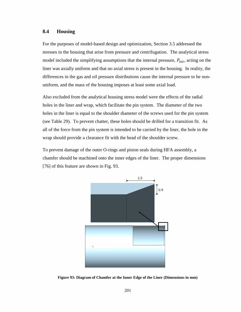
201

8.4 Housing

For the purposes of model-based design and optimization, Section 3.5 addressed the

stresses in the housing that arise from pressure and centrifugation. The analytical stress

model included the simplifying assumptions that the internal pressure, 𝑃𝑖𝑛𝑡, acting on the

liner was axially uniform and that no axial stress is present in the housing. In reality, the

differences in the gas and oil pressure distributions cause the internal pressure to be non-

uniform, and the mass of the housing imposes at least some axial load.

Also excluded from the analytical housing stress model were the effects of the radial

holes in the liner and wrap, which facilitate the pin system. The diameter of the two

holes in the liner is equal to the shoulder diameter of the screws used for the pin system

(see Table 29). To prevent chatter, these holes should be drilled for a transition fit. As

all of the force from the pin system is intended to be carried by the liner, the hole in the

wrap should provide a clearance fit with the head of the shoulder screw.

To prevent damage of the outer O-rings and piston seals during HFA assembly, a

chamfer should be machined onto the inner edges of the liner. The proper dimensions

[76] of this feature are shown in Fig. 93.

Figure 93: Diagram of Chamfer at the Inner Edge of the Liner (Dimensions in mm)

202

FEA has been carried out for the housing to confirm the analytical stress model used in

the design optimization. The analytical and FEA results are compared for the three

possible worst-case loading scenarios discussed in Section 3.5. These cases are

summarized in Table 30 for the selected laboratory prototype design, with the actual

observed pressures from a UDDS drive cycle simulation.

Table 30: The Three Potential Worst-case Loading Scenarios for the Housing

Case 1 Case 2 Case 3

Description high pressure, zero speed loss of pressure, high speed full SOC

𝑷𝒊𝒏𝒕,𝒐 [𝑴𝑷𝒂] 26.4 0 26.4

𝑷𝒊𝒏𝒕,𝒈 [𝑴𝑷𝒂] 26.4 0 26.4

𝝎 [𝒓𝒂𝒅/𝒔] 0 1154 1154

Failure Mode radial compressive, wrap radial tensile, wrap tensile, liner

Note that, for load case 3, the non-uniform pressure distribution is taken into account in

the FEA analysis. Given the nature of cases 1 and 2, the pressure distribution is, in fact,

uniform. The weight of the housing and the presence of the radial holes for the pin

system are also included in the FEA analysis. The maximum drive cycle torque, 𝑇𝑚𝑎𝑥, is

extremely small compared to the fluid pressure and centrifugal loading, and therefore

shear stresses due to angular acceleration have been omitted. Given the manufacturing

process for the housing, the interface between the liner and wrap is presumed to behave

as a bonded interaction.

Figures 94 through 96 show the radial, circumferential and von Mises stress distributions

as functions of radial position in the housing for the three potential worst cases. The

dotted data are the FEA results, and continuous curves are the analytical results. A

dashed vertical line marks the radial position of the interface between the liner and the

wrap (i.e. the position 𝑟𝑖 + 𝑡ℎ𝑙). For the FEA results, the data have been taken at an axial

position 3 cm inward from the gas side end cap. Examination of other axial positions

between the O-ring seals reveals little variation in the stress distributions, which lends

203

credit to the uniform pressure assumption used in the analytical model. At positions

outside the O-ring seals, fluid pressure does not act on the housing, and therefore the

stresses tend to be far lower.

Figure 94: Housing Stress Distributions for Case 1 (Zero Speed, High Pressure)

204

Figure 95: Housing Stress Distributions for Case 2 (Maximum Speed, Zero Pressure)

Figure 96: Housing Stress Distributions for Case 3 (Maximum Speed, High Pressure)

205

Figures 94 through 96 show excellent agreement between the FEA and analytical results,

especially in the wrap. Recall from Section 3.5 that the Tsai-Hill criterion, rather than the

von Mises criterion, is used to determine the safety factor of the wrap. Given the

definition of the Tsai-Hill criterion (see Eqn. 61), the agreement between the FEA and

analytical results with respect to the radial and circumferential stress distributions

suggests that the Tsai-Hill criterion has been accurately evaluated during the design

optimization. Additionally, note that the analytical von Mises stress distributions have

been calculated two-dimensionally. The agreement between the FEA and analytical

results with respect to the von Mises stress justifies the omission of axial stresses from

the analytical model. Based on the FEA results, axial stresses in the wrap are generally

compressive, and always 𝑂(1 𝑀𝑃𝑎) or less.

At low pressure and high speed (case 2, Fig. 95), the analytical model slightly under-

predicts the von Mises stresses in the liner. However, even based on the FEA results, the

safety factor still remains significantly above the constraint of 3 for this case. The

presence of the radial holes has a negligible impact on the stresses in the housing. More

complete FEA results for the housing are provided in Appendix E.

It should be mentioned that manufacturing with composites always involves considerable

uncertainties. In the case of the housing, it is very difficult to predict the nature of the

residual stresses that might be induced during the curing process [38], or to project the

time-dependent effects that might arise. Because the optimization presented in Section

7.4 did not drive the wrap to its largest allowable stress, the selected prototype design

exhibits a safety factor of 11.5 for the wrap. It is assumed that this is sufficiently

conservative to account for all of the uncertainties mentioned above. If possible, regular

monitoring of the structural health of the housing should be performed.

8.5 Axle

Section 3.2 presented methods for modeling stresses in and selecting proper dimensions

for the axle. Though these processes were developed for the purpose of model-based

206

design and optimization, they are fairly complete; the only features that have been

omitted until this point are small shoulders between the main section and the shafts that

prevent the stationary outer race of the bearings from contacting the rotating axle. The

diameter of these shoulders, which can be seen in the figures included in this section,

should be roughly equal to the outer diameter of the inner bearing race. They must be

axially long enough only to accommodate the small axial displacement of the races with

respect to one another. Given these considerations, the diameter and length of the

bearing shoulders are 1 cm and 0.5 mm, respectively.

FEA has been carried out to confirm that the methods used in the design optimization

have properly selected the various axle dimensions. Per the calculations detailed in

Section 3.2, a tensile axial force of 192 kN is applied to the areas where the axle contacts

the retainers. The gas and oil side shafts provide radial reactions to the eccentric force,

calculated in Section 3.6 to be 4.76 kN. Figure 97 shows two images the oil side of the

axle with annotations to various peak von Mises stress locations (stresses given in Pa).

Note that the maximum allowable stress, 𝑆𝑦,𝑎/𝑆𝐹, is 333 MPa.

From the top image in Fig. 97, it is clear that the seal diameter, 𝑑𝑠, has been properly

selected, as the peak stress near the radial port is equal to 𝑆𝑦,𝑎/𝑆𝐹. The top image of Fig.

97 also shows that the maximum stress in the oil side shaft is acceptable low (the probes

are located on the side which is in tensile bending). However, as seen in the bottom

image, the peak stress near the outer corner of the retainer groove exceeds the maximum

allowable stress, leading to a safety factor of only about 2. Because the stress here is

mostly compressive, this is deemed an acceptable stress concentration. The bottom

image also shows that the axle radius, 𝑟𝑎, has been properly selected, such that the peak

stress near the radial ports is about 𝑆𝑦,𝑎/𝑆𝐹. This is more thoroughly proven in Fig. 98,

which illustrates the von Mises stress along the radial line that coincides with the stress

concentration at the radial port.

207

Figure 97: FEA Results Near the Oil Side of the Axle, von Mises Stress (in Pa)

Figure 98: von Mises Stress in the Axle Along a Radial Line that Coincides with the Stress

Concentration at the Radial Port

208

Figure 99, which depicts the FEA results or the gas side of the axle, shows that the

maximum von Mises stress in the shaft is acceptably low.

Figure 99: FEA Results Near the Gas Side of the Axle, von Mises Stress (in Pa)

8.6 High-Speed Rotary Union Case

The purpose of the HSRU case is to form the outer part of the non-contacting

circumferential seal and to house the lower bearing. The design details of this component

have been omitted until now, as they have little bearing on the results of a design

optimization. A cross sectional view of the HSRU case, with all relevant dimensions, is

shown in Fig. 100.

Some details of the HSRU case are omitted here, as they depend on choices related to the

design of the containment chamber, which will be conducted by another researcher.

Namely, the mechanism by which the HSRU case is secured to the containment chamber

and the handling of the leakage oil must be addressed in the detailed design of the

chamber.

209

Figure 100: Cross-sectional View Illustrating the Dimensions of the High Speed Rotary Union

(HSRU) Case

To form the non-contacting circumferential seal, the bottom of the case has a through-

hole whose diameter is 2𝑐𝑠 larger than 𝑑𝑖, the diameter of the axle portion that protrudes

into the case. The length of this through-hole is equal to the seal length, 𝑙𝑠, plus a gap,

𝑐𝑔, that safely allows for thermal expansion of the axle. Above the circumferential seal is

an annulus of axial and radial dimensions 𝑑𝑙 into which leakage oil enters from the

circumferential seal. A radial leakage port of diameter 𝑑𝑙 allows oil to pass from the

leakage annulus to the inside of the containment chamber.

Above the leakage annulus is a secondary seal, the purpose of which is to further protect

the bearings from leakage oil. The secondary seal has a length of 𝑙2 and a clearance of

𝑐𝑔. At the top of the HSRU case is a groove that supports the lower bearing. The

diameter of this groove should create a press fit with the bearing, and the height should

allow a clearance of 𝑐𝑔 between the HSRU case and the main section of the axle.

The case thickness, 𝑡ℎ𝑐, must be large enough that the maximum expected eccentric

force, 𝐹𝑒𝑐𝑐, does not cause the material that forms the bearing pocket to shear off of the

210

case. It is assumed that the shear stress is distributed as if this material were a thin-

walled tube, where

𝜏𝑉,𝑐 =

2𝐹𝑒𝑐𝑐𝜋𝑑𝑏,𝑜𝑡ℎ𝑐

(243)

As was done in sizing the bearings, the maximum eccentric force is estimated using shaft

balancing standards and a safety factor of 10 (see Eqn. 65). Letting the shear stress in the

case go to its maximum allowable value, the case thickness should be

𝑡ℎ𝑐 =

2(𝑆𝐹)(𝑚 +𝑚𝑜)𝜔𝑚𝑎𝑥(10)6.3(10−3)

𝜋𝑑𝑏,𝑜(0.58)𝑆𝑦,𝑐 (244)

To avoid compressive failure of the circumferential face of the bearing groove, the

following inequality must be true

𝑆𝑦,𝑐

𝑆𝐹≥

12𝐹𝑒𝑐𝑐

12𝜋𝑑𝑏,𝑜(𝑤𝑏𝑟 − 𝑐𝑔)

=(𝑚 +𝑚𝑜)𝜔𝑚𝑎𝑥(10)6.3(10

−3)

𝜋𝑑𝑏,𝑜(𝑤𝑏𝑟 − 𝑐𝑔) (245)

Given the strength of gray iron, this inequality is easily satisfied for any reasonable set of

case dimensions.

System pressure acts inside the HSRU case only between the containment chamber and

the bottom of the axle. Because the non-contacting circumferential seal diameter is much

smaller than the outer diameter of the bearing, it is assumed that this pressure does not

create a critical stress, and therefore Eqn. 244 drives the outer diameter of the HSRU case

to an appropriate value.

Because the HSRU case must interface with the containment chamber, which is outside

the scope of this thesis project, actual values for 𝑡ℎ𝑐, 𝑐𝑔, and 𝑙2 are not specified here. In

general, the HSRU case can be overdesigned, as it is a relatively low-cost and low-mass

component. For the laboratory prototype, the outer diameter of the HSRU case may be

driven by the dimensions of gray iron roundstock that is convenient to procure.

Recall from Eqns. 114 and 116 that some amount of heat is generated in the

circumferential seal formed by the HSRU case and the portion of the axle that protrudes

into it. The design process described in Section 3.2 has prescribed a seal diameter, 𝑑𝑠, of

211

5.9 mm to withstand the system pressure acting inside the axle. The resultant wall

thickness of the axle at the circumferential seal is only 0.25 mm thick, and therefore may

be prone to significant thermal expansion. It is necessary to confirm that radial thermal

expansion of the axle will not cause it to bind with the HSRU case. Since the thermal

capacitance of the HSRU case should be relatively large, binding is particularly likely to

happen during startup, when the small portion of the axle that protrudes into the case

rapidly heats up.

A simple finite-difference computational heat transfer code has been developed to

analyze the transient behavior of the circumferential seal at startup. Because this is an

axisymmetric problem, the numerical scheme is spatially 2-dimensional. The

computational domain includes both the fluid region and the portion of the axle that

forms the circumferential seal, as depicted in Fig. 101. Arrows indicate the leakage flow

of oil (that which passes through the circumferential seal).

Figure 101: Computational Domain and Boundary Conditions for the Heat Transfer Analysis of the

Circumferential Seal

The fluid mechanics problem for this flow case has a closed-form analytical solution that

was derived in Section 4.3. The fluid velocity profiles and volumetric rate of heat

generation within the seal are therefore already known (and assumed to be fully-

developed at startup), and the numerical scheme need only include the energy equation.

212

At each time step, the temperature distribution in the oil portion of the computational

domain is solved for first, and the temperature distribution along the bottom of this

portion is used as the boundary condition for the axle at the seal diameter. It is assumed

that the oil entering the seal (the leakage oil) and the oil inside the axle is at a constant

40° C, typical for a hydraulic system. Heat that is generated in the seal can be convected

to the HSRU case or to the axle. Because the HSRU case is attached to the containment

chamber, which is metal, it is modeled as an infinite heat sink at a temperature of 40° C.

Heat can be conducted axially through the axle to the storage PM, which is assumed to be

a heat sink at a temperature of 50° C. The thermal resistance of the conduction path

through the axle, 𝑅𝑎, is approximated as a series of 1-dimensional resistances, calculated

by breaking the distinct portions of the axle into simple cylindrical segments. At the

bottom border of the computation domain, heat can also be conducted back to the oil

within the axial port, which is modeled as stagnant at a constant 40° C. A Neumann

boundary condition is used on the temperature of the oil exiting the circumferential seal.

Because the HSRU case is modeled as a sink, its geometry does not change. The seal

diameter changes throughout the transient simulation by the equation

𝑑𝑠𝑖 = 𝑑𝑠,𝑜[1 + 𝛼𝑠,𝑠(�̅�𝑠

𝑖 − 𝑇𝑠,𝑜)] (246)

where 𝑑𝑠,𝑜 is the initial seal diameter (assumed to be axially constant), 𝛼𝑠,𝑠 is the thermal

diffusivity of steel, �̅�𝑠𝑖 is the temperature at the axial location 𝑖, averaged across the radial

dimension of the axle, and 𝑇𝑠,𝑜 is the initial temperature of the axle. The former is set to

be a spatially-uniform 40° C. Changes in the seal diameter are reflected in the step sizes

of the computational domain, which in turn impact the fluid velocity profiles. The

complete code can be found on pg. 280 in Appendix B.

The numerical scheme described above has been implemented for the specific

dimensions of the selected laboratory prototype. The initial seal clearance must be made

greater than 10.2 μm (the value specified by the optimization) in order to accommodate

the radial growth of 𝑑𝑠. By trial and error, an initial clearance of 15 μm has been selected

as an appropriate value. Figure 102 shows the steady-state seal clearance as a function of

axial position in the seal.

213

Figure 102: Steady-state Seal Clearance Distribution vs. Axial Position

Note that the initial clearance selected here has produced an average steady state clearace

of 11.5 μm. This is deemed sufficiently close to the desired seal clearance of 10.2 μm.

The results of this computational heat transfer study also indicate that the temperature of

the leakage oil never exceeds 75° C. This ensures that the oil will not degrade.

8.7 Relative Radial Strain Analysis

The HFA components are manufactured such that, at assembly, there is some radial

clearance at each interface between concentric components. Throughout various

operating states, changes in pressure and/or centrifugal forces cause these radial

clearances to fluctuate. The purpose of this section is to analyze the relative radial strains

of the axle, end caps, housing and piston. Properly specifying the clearances between

these components at assembly will ensure the integrity of the piston and O-ring seals

throughout the entire range of expected operating conditions.

For the purposes of evaluating relative radial strains, the axle, end caps, housing and

piston are modeled as simple cylinders, ignoring the effects of any minor design features

(e.g. radial ports in the axle, radial holes in the housing, O-ring glands). Each component

0 1 2 3 4 5 6 7 8 911

11.2

11.4

11.6

11.8

12

axial position (mm)

seal cle

ara

nce d

istr

ibution (

m)

214

is presumed to deform axisymmetrically with no end effects. Because of their low

stiffness, the seals themselves (O-rings and piston seals) impose negligible radial loads.

In the case of the end caps and piston, radial strain due to bending is ignored.

Radial strain is presumed to arise only due to centrifugal forces and fluid pressure acting

radially on the components of interest. Equations 47 and 48 described the radially-

dependent stress distributions in a homogenous, isotropic, thick-walled cylinder exposed

to internal, external, and/or centrifugal loading. These equations are used for the axle,

end caps and piston. Section 3.5 detailed the equivalent calculations for a hybrid cylinder

with anisotropic mechanical properties, which are applied to the housing. Whether

isotropic or anisotropic, the stress distributions in a cylinder can be converted to a

circumferential strain distribution by

𝜖𝑐(𝑟) =

1

𝐸𝑚[𝜎𝑐(𝑟) − 𝜈(𝜎𝑟(𝑟) − 𝜎𝑧)] (247)

which, in turn, can be converted to a radial displacement distribution by

𝛿𝑟(𝑟) = 𝑟𝜖𝑐(𝑟) (248)

In Eqn. 247, 𝜎𝑐, 𝜎𝑟 and 𝜎𝑧 are the circumferential, radial and axial stresses, 𝐸𝑚 is the

elastic modulus and 𝜈 is the Poisson ratio (in the case of an anisotropic material, the

longitudinal Poisson ratio, 𝜈𝐿). Notice that the axial stress is presumed to be constant at

all radial locations. As before, the housing is modeled as free of any axial stresses.

The remainder of this section justifies the worst-case scenarios for each sealing interface

and presents the corresponding expected range of radial clearances. For a given

interface, once the worst-case radial displacement distributions for each component have

been calculated, the maximum expected change in the clearance is simply the difference

between the outer and inner displacements, 𝛿𝑟, evaluated at the radius of the interface.

Note that nominal dimensions (those presented in Tables 25 and 26) are used for the

present analysis, even though one of the primary purposes of this section is to specify

more precise dimensions. While an iterative process could be used to address this issue,

it is assumed that using nominal dimensions rather than the final selected dimensions

introduces negligible error in the prediction of radial strain.

215

As described in Sections 3.4 and 8.3, two piston seals are used between the piston and the

housing, and two rod seals are used between the piston and the axle. The clearances at

these interfaces must not grow so much that the seals are prone to leakage and must not

shrink so much that the components bind, preventing translation. The particular seals

selected for the prototype can accommodate a 43.5 μm range of radial clearances [32].

At the interface between the axle and piston, only the bearing length of the piston is

considered; effects due to the disc section of the piston are neglected. The axle is

modeled as a solid infinite cylinder. Recall that the piston is made of aluminum and the

axle is made of steel. Given these material selections and the fact that the axle is at a

smaller radius, the piston should be more heavily affected by centrifugal forces. This

interface, therefore, is most prone to leakage at 𝜔𝑚𝑎𝑥, and the separation between the

components should be exacerbated when there is a loss of pressure. Table 31

summarizes the loads and resultant radial displacements for the worst-case leakage

scenario.

Table 31: Loads and Radial Displacements for the Worst-case Leakage Scenario at the Axle-Piston

Interface

Loading

Pressure outside of piston 0

Pressure acting within seal 0

Axial stress in piston 0

Axial stress in axle 0

Angular velocity 1154 rad/s

Displacements

Axle 0.12 μm

Piston 2.2 μm

Net 2.1 μm

The worst case from the perspective of binding occurs when centrifugal forces are absent,

the HFA is pressurized, and no pressure is acting in the seal between the piston and axle.

This scenario occurs, for example, when the HFA is charged. To be conservative, the

maximum observed pneumatic pressure during drive cycle simulation is used here. The

loads and radial displacements for this binding scenario are summarized in Table 32.

216

Table 32: Loads and Radial Displacements for the Worst-case Binding Scenario at the Axle-Piston

Interface

Loading

Pressure outside of piston 26.4 MPa

Pressure acting within seal 0

Axial stress in piston -26.4 MPa

Axial stress in axle 106.1 MPa


Displacements

Axle -3.6 μm

Piston -21.7 μm

Net -18.1 μm

Examining the results in Tables 31 and 32, the difference between the maximum growth

and maximum shrinkage of the clearance at the axle-piston interface is expected to be

20.2 μm. This is well within the acceptable range of 43.5 μm. Manufacturing the piston

to have an inner radius 10 μm larger than the axle radius, 𝑟𝑎, should safely allow for the

relative radial strain of these components.

The other location at which the piston creates a seal is at its interface with the liner of the

housing. For the present analysis, the effects of the bearing section of the piston are

neglected, such that it can be modeled as a simple cylinder of axial length 𝑡ℎ𝑝 and inner

and outer radii 𝑟𝑎 and 𝑟𝑖, respectively. By virtue of their different material properties, the

housing has a higher specific modulus than the piston. However, because its mass is

concentrated at a larger radius, the housing experiences a stronger centrifugal field. It is

not clear, then, which component will exhibit more radial displacement due to centrifugal

effects. Therefore, two potential worst-case scenarios for leakage must be analyzed.

If centrifugation tends to create larger displacements in the piston, leakage is most likely

at zero speed and maximum pressure. If, on the other hand, centrifugation causes larger

displacements in the housing, leakage is most likely at maximum speed and maximum

pressure. For both of these potential worst-case leakage scenarios, it is assumed that

pressure acts in the seals between the piston and housing and between the piston and axle.

In the zero speed case, the maximum observed value of 𝑃𝑝 is used for both the pressure

acting on the housing and the compressive axial stress in the piston. For the maximum

217

speed case, the maximum observed value of 𝑃𝑖𝑛𝑡,𝑜 is used as the pressure on the housing,

and the corresponding value of 𝑃𝑝 is used for the axial piston stress. The two worst-case

leakage scenarios, along with their resultant radial displacements, are summarized in

Table 33.

Table 33: Loads and Radial Displacements for the Worst-case Leakage Scenarios at the Piston-

Housing Interface

Case 1

Loading

Pressure acting on the housing liner 26.4 MPa

Pressure acting within piston-housing seal 26.4 MPa

Pressure acting within piston-axle seal 26.4 MPa


Angular velocity 0

Displacements

Piston -16.5 μm

Housing 40.4 μm

Net 20.9 μm

Case 2

Loading


Pressure acting within piston-housing seal 26.4 MPa




Displacements

Piston -13.8 μm

Housing 49.1 μm

Net 27.0 μm

The piston and housing are most prone to binding when pressure acts in the seal between

the axle and piston but not between the piston and housing. While this condition is

unlikely, it is conservative to use it as a worst-case assumption. There are two potential

worst-case scenarios from the perspective of binding. The first is when the maximum

observed value of 𝑃𝑜(𝑟𝑎) acts between the axle and piston. For this case, the

corresponding values of 𝜔𝑠, 𝑃𝑝, and 𝑃𝑖𝑛𝑡,𝑜 are used as the angular velocity, the axial stress

in the piston, and the pressure acting on the housing. The other worst-case scenario for

binding occurs when the HFA is charged, with 𝑃𝑐 acting between the axle and piston and

218

imposing axial stress in the piston. Angular velocity is zero when the HFA is charged.

The two potential worst-case scenarios for binding are summarized in Table 34.

Table 34: Loads and Radial Displacements for the Worst-case Binding Scenarios at the Piston-

Housing Interface

Case 1

Loading


Pressure acting within piston-housing seal 0



Angular velocity 128.2 rad/s

Displacements

Piston 42.4 μm

Housing 40.5 μm

Net -1.9 μm

Case 2

Loading


Pressure acting within piston-housing seal 0



Angular velocity 0

Displacements

Piston 26.3 μm

Housing 25.0 μm

Net -1.3 μm

Given the results from Tables 66 and 34, the maximum expected range of radial

clearances between the piston and housing is 28.3 μm, well within the acceptable range.

To accommodate the expected relative radial strains, the piston should be manufactured

such that its outer radius is 10 μm less than the inner radius of the liner, 𝑟𝑖. Note that the

maximum expected growth of the clearance between the piston and housing increases

significantly if pressure does not act between the axle and piston. To ensure this scenario

does not occur, the HFA should be charged and the piston forced to translate some

distance (thereby introducing pressurized fluid between the rod seals) before any angular

velocity is imposed.

219

Like the piston, the end caps seal against the axle and the housing. Based on the SAE

AS5857 O-ring standard [76], the maximum allowable clearance at these interfaces is

63.5 μm. Because the end cap seals are non-translational interfaces, however, shrinkage

(even to zero) of the clearances is acceptable; it is assumed that any compressive

interaction between the end caps and the axle or housing induces stresses that are

insignificant compared to the other HFA loads.

With respect to the interface between the end caps and axle, the gas side end cap in

particular is more prone to leakage, since the axle is solid near this interface. Because the

end cap has a lower specific modulus and is exposed to a larger centrifugal field than the

axle, leakage is most likely at high pressure and maximum speed. The maximum

observed value of 𝑃𝑜(𝑟𝑎) acts to compress the axle, but because the O-ring seal is located

near the inner face, it is assumed that no pressure acts at the inner or outer periphery of

the end cap. The axial stress in the axle is calculated using Eqn. 35 at the maximum

observed 𝑃𝑝, and the end cap is assumed to be free of any axial stress. These worst-case

loads and the resultant displacements of the axle and end cap are summarized in Table

35.

Table 35: Loads and Radial Displacements for the Worst-case Leakage Scenario at the Axle-End

Cap Interface

Loading

Pressure acting on axle 26.4 MPa

Axial stress in axle 106.8 MPa


Displacements

Axle -5.7 μm

End cap 3.1 μm

Net 8.8 μm

The maximum expected growth of the clearance between the end caps and housing must

also be checked. Leakage here is most likely at high pressures, when the housing is

highly-strained. As in the case of the piston and housing, it is unclear which component

will experience greater deformation due to centrifugal effects. The worst-case scenario

for leakage between the end caps and housing, then, occurs either at high speed and high

220

pressure or at zero speed and high pressure. Table 36 summarizes these two cases, along

with the resultant displacements of the end caps and housing.

Table 36: Loads and Radial Displacements for the Worst-case Leakage Scenarios at the End Cap-

Housing Interface

Case 1

Loading



Displacements

End cap 2.7 μm

Housing 49.1 μm

Net 46.4 μm

Case 2

Loading


Angular velocity 0

Displacements

End cap 0

Housing 40.4 μm

Net 40.4 μm

Given the results of this study on relative radial strains, the piston, rod and O-ring seals

used in the laboratory prototype should remain robust throughout the entire range of

operating conditions. It should be noted that many of the cases examined were specified

very conservatively by assuming, for example, that some maximum pressure can occur

simultaneously with maximum HFA angular velocity. Observations from the UDDS

drive cycle simulation suggest, in fact, that the maximum pressures tend to occur near

low angular velocities. It is difficult to project how the piston and rod seals will behave

under the influence of centrifugal forces. This issue may require special attention during

the initial testing of the prototype.

221

9 Conclusions and Recommendations

This chapter begins by a restatement of the motivation for the work presented in this

thesis. Next, a summary of the primary methods used to evaluate the HFA concept is

provided, and important results are reviewed. The chapter concludes with

recommendations for future research.

9.1 Summary of the Research

Hydraulic systems offer an inexpensive, power dense and robust means of power delivery

and motion control. The low energy density of traditional hydraulic energy storage

media, however, is an impedance to the widespread adoption of hydraulic power for

mobile applications. This thesis has shown that, by combining hydro-pneumatic and

rotating kinetic energy storage into one device, the hydraulic flywheel-accumulator has

the potential to vastly improve the energy storage density of hydraulic systems. A simple

control strategy has also been devised to illustrate the ability of the HFA to operate at

near-constant system pressure. This offers the opportunity to downsize the peripheral

components of the hydraulic system, reducing both cost and mass.

Model-based design is the primary means by which this thesis has assessed the potential

performance capability of the HFA. Relatively simple and robust models for mechanical

stress and energy exchange have been developed and integrated, forming a toolset that

facilitates the performance modeling of candidate HFA designs. To minimize the

computational expense of the model-based design process, special effort has been put

towards developing a simple empirical model of the rotating fluid behavior. As a result,

the HFA performance for a 20 minute drive cycle can be completed on the order of one

second. The aforementioned toolset has been embedded into a multi-objective

optimization scheme which uses a genetic algorithm to find a set of HFA designs with

minimal mass and energy losses.

222

9.2 Conclusions

Minimizing of the HFA system mass and drive cycle losses have been identified as the

two primary objectives in the design of the HFA. As discussed in Chapter 7, the multi-

objectivity of the optimization problem yields a set of Pareto-optimal solutions. At one

extreme end of the PO set, the solutions are small, fast-spinning and very energy dense.

These flywheel-like solutions tend to have fairly small pneumatic energy capacities

which, in combination with their high angular velocities, lead to relatively high drive

cycle losses.

At the other extreme end of the PO set are slower-spinning and larger solutions, which

more closely resemble traditional accumulators. Their lower angular velocities mitigate

rotation-depenent losses, and their larger dimensions lead to higher pneumatic energy

capacity, thereby decreasing dependence on the inefficient kinetic domain. The

flywheel- and accumulator-like extremes of the PO front are bridged by a continuum of

intermediate solutions, offering a diverse range of potential solutions for a specified HFA

application.

Results from the optimizations presented in Chapter 7 indicate that, given the constraints

imposed by a passenger vehicle-scale application, the HFA can achieve an energy density

of more than 31 kJ/kg, operating at over 76% efficiency. Even with generous estimates

of static accumulator energy density, this represents at least a six-fold improvement in the

energy storage density of hydraulic systems. Setting more modest goals, the energy

density can be doubled (10 kJ/kg) over traditional hydraulic storage media while

operating at around 88% efficiency.

The achievable energy density at the laboratory scale is somewhat lower, owing to the

inherent correlation between energy density and energy capacity for the HFA

architecture. The improvement over static accumulator energy storage, however, is more

pronounced. Subject to realistic packaging constraints for a small laboratory, the HFA

offers at least an eleven-fold advantage in energy density over a static accumulator. The

primary cause of drive cycle losses is the inefficiency of the storage PM, which

contributes between 80% and 90% of losses at the vehicle scale and between 60% and

223

75% at the laboratory scale. This can be viewed as a promising statistic, as it indicates

that none of the energy loss mechanisms that are unique (at least within the field of

hydraulic energy storage) to the HFA concept are prohibitively large.

In evaluating the merits of the HFA concept, it is important to consider the benefits of the

decoupling between system pressure and SOC. While it has not been included in the

design optimization as an explicit objective or constraint, minimization of system

pressure fluctuation indirectly serves to minimize the mass of the hydraulic system. The

traction PM in a hydraulic powertrain must be sized to produce adequate flow rate to

meet power demands at the minimum system pressure during a drive cycle. At both the

vehicle and laboratory scales, the more accumulator-like solutions are able to limit the

fluctuation of system pressure to within a 10% band about the design pressure. As a

result, the traction pump-motors for these solutions need only be 4% heavier than they

would be if system pressure remained perfectly constant throughout the entire drive

cycle. This type of operation represents a distinct advantage over a traditional static

accumulator, whose minimum SOC pressure may be as much as 63% lower than the

design pressure [18], requiring significant oversizing of the traction PM.

A particular HFA design solution, whose characteristics are summarized in Tables 25

through 28, has been selected from the laboratory-scale optimization results. This

solution has been subject to a detailed design process and is recommended to be built as a

laboratory prototype. As a part of the detailed design process, all of the stress models

used in the rapid performance assessment toolset have been validated using FEA.

Various minor design features that were neglected during the design optimization have

been addressed in detail, and most hardware has been specified. The laboratory

prototype is projected to have an energy density of 8.8 kJ/kg and be capable of achieving

a drive cycle efficiency of 87%.

224

9.3 Future Work

The details of numerous design features that are outside the scope of this thesis project

will need to be addressed in the construction of the laboratory prototype and its test rig.

After construction, for example, the laboratory prototype may require dynamic balancing.

It is recommended that a professional balancing service provider perform this operation,

should it be deemed necessary. The containment chamber must provide adequate

protection for the experimentalists and facilitate easy service and maintenance.

Additionally, a convenient process of removing leakage oil and applying vacuum to the

chamber must be devised. To validate the models developed in this research and to prove

the HFA concept, the prototype HFA should be interfaced with a hydraulic power system

that is capable of simulating the transient tractive loads of a passenger vehicle. The

details of this system, including the control scheme, are outside the scope of the presented

work.

The recommended testing procedure is to drive the HFA through some power profile,

measuring angular velocity, torque, piston position, pneumatic pressure, and hydraulic

system pressure. The exact applied power profile should then be used as the input to the

simulation toolset detailed in this thesis. The experimental and simulated results can be

compared and the performance models adjusted as necessary. More accurate models will

improve the robustness of future design optimization results.

In experimentally validating the HFA performance, several areas are of particular

interest, as they have not been thoroughly addressed in this thesis. First, the fluid model

detailed in Chapter 5 is truly applicable only to the specific geometry and working fluid

with which it was developed. Second, the present model does not address the presumed

exchange of kinetic energy between the oil and the solid HFA components when the

pneumatic domain is charged or discharged. The HFA prototype should be used, in part,

to expand upon the simple fluid model, such that it encompasses all reasonable HFA

geometries and accounts for the extraction and addition of oil.

Some phenomena that are irrelevant for the recommended laboratory prototype may

become important at the vehicle scale. Gyroscopic torque, for example, is a non-issue for

225

a stationary prototype, but in a passenger vehicle application it may affect the handling of

the vehicle. The mounting orientation of the HFA has implications on which axes of the

vehicle will be impacted by gyroscopic effects, and the size and rotational speed of the

HFA dictate the magnitude. These should all be carefully considered when designing an

HFA for a vehicle application.

The design goals for the containment chamber are also application-dependent. In the

case of a laboratory prototype, the containment chamber can be heavily over-designed

without significant negative impacts. For a passenger vehicle, however, the specification

of the containment chamber should involve an optimization and detailed design process

in itself. Namely, the chamber must not add an appreciable amount of mass to the HFA

system, and its packaging volume must be non-intrusive to the passengers of the vehicle.

The challenges of containment and gyroscopic effects are not unique to the present

research; previous successful flywheel powertrain integrations can serve as guiding

examples for HFA vehicle applications.

Finally, it should be emphasized that many of the fundamental decisions documented in

this thesis have been made within the context and the constraints of academic research. It

is possible that an improvement in HFA performance can be realize by altering some of

these decisions. The end caps, for example have been specified as cylindrical

components, simple to model and fabricate. Using hemispherical end caps would likely

allow for the end cap mass to be further minimized. Similarly, given the complex nature

of composite materials, the design of the housing may offer some opportunity for further

optimization.

Even the architecture itself has been selected for its compatibility with model-based

design; the free-floating end cap provides a simple loading case on the housing,

eliminating axial stresses and facilitating a robust analytical stress model.

Fundamentally-different architectures may offer advantages, albeit with the penalty of

more costly and time-consuming design processes. Control strategy sophistication, too,

can potentially effect a drastic improvement in the dynamic performance characteristics

of the HFA.

226

Clearly, there is ample opportunity for further research and improvement of the HFA

concept. However, the results of this early research are extremely promising. Even

having made various concessions based on the present scope and constraints, it is

projected that the HFA exhibits an order of magnitude higher energy density than static

accumulator storage, while offering constant or near-constant pressure operation. These

drastic improvements can enhance the performance of current mobile hydraulic systems

and promote further adoption of hydraulics for vehicular propulsion.

227

Bibliography

[1] Solomon, S., Qin, D., Manning, M., Marquis, M., Averyt, K., Tignor, M., Miller, H. L.

and Chen, Z., 2007, “Climate Change 2007: The Physical Science Basis,” Cambridge

Univeristy Press, New York, NY.

[2] McMichael, A. J., Woodruff, R. E. and Hales, S., 2006, “Climate Change and Human

Health: Present and Future Risks,” The Lancet, 367, 859-869.

[3] Zhang, K., Douglas, B. C. and Leatherman, S. P., 2004, “Global Warming and

Coastal Erosion,” Climate Change, 64(1), pp. 41-58.

[4] Malcom, J. R., Liu, C., Neilson, R. P., Hansen, L. and Hannah, L., 2006, “Global

Warming and Extinctions of Endemic Species From Biodiversity Hotspots,”

Conservation Biology, 20(2), pp. 538-548.

[5] 2014, “Inventory of U.S. Greenhouse Gas Emissions and Sinks: 1990-2012,” U.S.

Environmental Protection Agency, Washington, DC.

[6] Metz, B., Davidson, O., Bosch, P., Rutu, D. and Meyer, L., 2007, “Climate Change

2007: Mitigation of Climate Change,” Cambridge Univeristy Press, New York, NY.

[7] Kintner-Meyer, M., Schneider, K. and Pratt, R., 2007, “Impacts Assessment of Plug-

In Hybrid Electric Vehicles on Electric Utilities and Regional US Power Grids Part I:

Technical Analysis,” Pacific Northwest Laboratory, Richland, WA.

[8] Goering, C., Stone, M., Smith, D., Turnquist, P., 2006, Off-Road Vehicle Engineering

Principles, American Society of Agricultural Engineers, St. Joseph, MI, Chaps. 2, 4.

[9] Parks, K., Denhold, P. and Markel, T., 2007, “Costs and Emissions Associated with

Plug-In Hybrid Electric Vehicle Charging in the Xcel Energy Colorado Service

Territory,” NREL/TP-640-41410, National Renewable Energy Laboratory, Golden, CO.

[10] Westbrook, M. H., 2001, The Electric Car: Development and Future of Battery,

Hybrid and Fuel-Cell Cars, The Institution of Engineering and Technology, London, UK.

[11] Lorenz, R. D. and Haines, L. P., 2000, Understanding Modern Power Conversion.

[12] Sclater, N., 1999, Electronic Technology Handbook, McGraw-Hill, New York, NY.

[13] Burke, A., 2000, “Ultracapacitors: Why, How, and Where is the Technology,” J.

Power Sources, 91, pp. 37-50.

[14] Frank, A. A. and Beachley, N. H., 1979, “Evaluation of the Flywheel Drive Concept

for Passenger Vehicles,” No. 790049, SAE Technical Paper.

228

[15] Green Car Congress, 2014, “Ricardo TorqStor Flywheel Energy Storage Technology

Recieves SAE 2014 World Congress Tech Award,” from

http://www.greencarcongress.com/2014/04/20140401-torqstor.html.

[16] Filipi, Z., Louca, L., Daran, B., Lin, C.-C., Yildir, U., Wu, B., Kokkolaras, M.,

Assanis, D., Peng, H., Papalambros, P., Stein, J., Szkubiel, D. and Chapp, R., 2004,

“Combined Optimisation of Design and Power Management of the Hydraulic Hybrid

Propulsion System for the 6 x 6 Medium Truck,” Int. J. of Heavy Vehicle Systems,

11(3/4), pp. 372-402.

[17] Flippo, W. and Rajabi, B., 2008, “Reduce Hydraulic Accumulator Cost with Back-

Up Gas Bottles,” from http://www.designworldonline.com/reduce-hydraulic-

accumulator-cost-with-back-up-gas-bottles.

[18] Li, P. Y., Van de Ven, J. D. and Sancken, C. S., 2007, “Open Accumulator Concept

for Compact Fluid Power Energy Storage,” Proceedings of the ASME International

Mechanical Engineering Congress, Seattle, WA, pp. 127-140.

[19] Pourmovahed, A., Baum, S. A., Fronczak, F. J., and Beachley, N. H., 1988,

“Experimental Evaluation of Hydraulic Accumulator Efficiency With and Without

Elastomeric Foam,” J. Propulsion, 4(2), pp. 185-192.

[20] Sherman, M. P. and Karlekar, B. V., 1973. “Improving the Energy Storage Capacity

of Hydraulic Accumulators,” Proceeding of the AIAA 8th Intersociety Energy Conversion

Engineering Conference, pp. 202–207.

[21] Pedchenko, A. and Barth, E. J., 2009, “Design and Validation of a High Energy

Density Elastic Accumulator Using Polyurethane,” ASME Dynamic Systems and Control

Conference, Hollywood, CA, pp. 283-290.

[22] Tucker, J. M. and Barth, E. J., 2013, “Design, Fabrication, and Evaluation of a

Distributed Piston Strain-Energy Accumulator,” Intl. J. Fluid Power, 14(1), pp. 47-56.

[23] Van de Ven, J. D., 2009, “Increasing Hydraulic Energy Storage Capacity: Flywheel-

Accumulator,” Intl. J. Fluid Power, 10(3), pp. 41-50.

[24] Norton, R. L., 2008, Design of Machinery, McGraw-Hill, New York, NY, pp.72-73,

Chap. 2.

[25] Genta, G., 1985, Kinetic Energy Storage, Butterworths, Cambridge, UK, pp. 55-67,

Chap. 3.

[26] Pourmovahed, A., Beachley, N. H. and Fronczak, F. J., 1992, “Modeling of a

Hydraulic Energy Regeneration System – Part I: Analytical Treatment,” J. Dynamic

Systems, Measurement and Control, 114, pp. 155-159.

229

[27] Gillespie, T. D., 1992, Fundamentals of Vehicle Dynamics, Society of Automotive

Engineers, Inc., Warrendale, PA, pp. 111-118, Chap. 4.

[28] Juvinall, R. C., and Marshek, K. M., 2006, Fundamentals of Machine Component

Design, Wiley, Hoboken, NJ, pp. 406-417, Chap. 10.

[29] Young, W. C., and Budynas, R. G., 2002, Roark’s Formulas for Stress and Strain,

McGraw-Hill, New York, NY, pp. 457-475, Chap. 11.

[30] Timoshenko, S., 1940, Theory of Plates and Shells, McGraw-Hill, New York, NY,

pp. 55-75, Chap. 3.

[31] Heap, J. C., 1964, “Bending of Circular Plates Under a Uniform Load on a

Concentric Circle,” ANL-6905, Argonne National Lab, Argonne, IL.

[32] 2012, “2012 Seal Catalog,” Hercules Sealing Products, Clearwater, FL.

[33] Perez-Aparicio, J. L. and Ripoll, L., 2011, “Exact, Integrated and Complete

Solutions for Composite Flywheels,” J. Composite Structures, 93, pp. 1404-1415.

[34] Ha, S. K., Kim, S. J., Nasir, S. U. and Han, S. C., 2012, “Design Optimization and

Fabrication of a Hybrid Composite Flywheel Rotor,” J. Composite Structures, 94, pp.

3290-3299.

[35] Ha, S. K., Kim, D. and Sung, T., 2001, “Optimum Design of a Multi-ring Composite

Flywheel Rotor Using a Modified Generalized Plain Strain Assumption,” Intl. J.

Mechanical Sciences, 43, pp. 993-1007.

[36] Arvin, A. C. and Bakis, C. E., 2006, “Optimal design of Press-fitted Filament

Wound Composite Flywheel Rotors,” J. Composite Structures, 72, pp. 47-57.

[37] Arnold, S. M., Saleeb, A. F. and Al-Zoubi, N. R., 2002, “Deformation and Life

Analysis of Composite Flywheel Disk Systems,” J. Composites, 33, pp. 433-459.

[38] Portnov, G., Uthe, A.-N., Cruz, I., Fiffe, R. P. and Arias, F., 2005, “Design of Steel-

composite Multirim Cylindrical Flywheels Manufactured by Winding with High

Tensioning and In Situ Curing. 1. Basic Relations,” Mechanics of Composite Materials,

41(2), pp. 139-152.

[39] Wild, P. M. and Vickers, G. W., 1996, “Analysis of Filament-wound Cylindrical

Shells Under Combined Centrifugal, Pressure and Axial Loading,” J. Composites, 28A,

pp. 47-55.

[40] Staab, G., 1999, Laminar Composites, Butterworth-Heinemann, Woburn, MA.

[41] International Organization for Standardization, 2003, “Mechanical Vibration –

230

Balance Quality Requirements for Rotors in a Constant (Rigid) State,” 1940-1.

[42] Bamberger, E. N., Zaretsky, E. V. and Signer, H., 1975, “Effect of Speed and Load

on Ultra-high-speed Ball Bearings,” NASA TN D-7870, Lewis Research Center,

Cleveland, OH.

[43] “High Precision Ball Bearings,” 4000 0805, GMN Paul Muller Industrie GmbH &

Co. KG, Numberg, Germnay.

[44] Smith, C., 1984, Engineer to Win, MBI, Osceola, WI, Chap. 3.

[45] 2014, “Online Materials Information Resource,” from www.matweb.com.

[46] Bhushan, B., 2002, Introduction to Tribology, Wiley, Hoboken, NJ.

[47] Houpert, L., 2002, “Ball Bearing and Tapered Roller Bearing Torque: Analytical,

Numerical and Experimental Results,” Tribology Transactions, 45(3), pp. 345-353.

[48] 2013, “Rolling Bearings,” CAT. No. E1102m, NSK Motion and Control, Japan.

[49] 2009, “Ball and Roller Bearings,” Catalog A-1000-XI, NTN, Mt. Prospect, IL.

[50] Stoneburner, M., 2005, “Hybrid Ceramic Bearings: More Mettle than Metal,” Plant

Engineering.

[51] Gorland, S. H., Kempke, E. E., Jr. and Lumannick, S., 1970, “Experimental

Windage Losses for Close Clearance Rotating Cylinders in the Turbulent Flow Regime,”

NASA TM X-52851, Lewis Research Center, Cleveland, OH.

[52] Etemad, M. R., Pullen, K., Besant, C. B., and Baines, N., 1992, “Evaluation of

Windage Losses for High-Speed Disc Machinery,” Proc. Instn. Mech. Engrs., Part A: J.

Power and Energy, Vol. 206, pp. 149-157.

[53] 2000, “A Descriptive Summary of Vickers Inline Pumps and their Applications,”

SE-103F, Vickers Fluid Systems, Jackson, MS.

[54] Pourmovahed, A., Beachley, N. H. and Fronczak, F. J., 1992, “Modeling of a

Hydraulic Energy Regeneration System – Part II: Experimental Program,” J. Dynamic

Systems, Measurement and Control, 114, pp. 160-165.

[55] Nellis, G. and Klein, S., 2009, Heat Transfer, Cambridge University Press, New

York, NY.

[56] American National Standards Institute, 1985, “Surface Texture,” B46.1-1985.

[57] White, F. M., 2008, Fluid Mechanics, McGraw-Hill, New York, NY, pp. 382-386,

Chap. 6.

231

[58] Johnson, M. L., Manos, D. M. and Provost, T., 1997, “Gas Permeation and Leakage

Through Reusable Seals,” J. Vac. Sci. Technol. A, 15(3), pp. 763-767.

[59] Rack, P. D., “Pumpdown and Vacuum Pumps,” lecture slides.

[60] Umrath, W., 2007, “Fundamentals of Vacuum Technology,” Oerlikon Leybold

Vacuum, Cologne, Germany.

[61] Moran, M. J. and Shapiro, H. N., 2008, Fundamentals of Engineering

Thermodynamics, Wiley, Hoboken, NJ, p. 308, Chap. 6.

[62] Chiggiato, P., 2006, “Outgassing,” Vacuum in Accelerators Conference, Platja

d’Aro, Spain.

[63] Perkins, W. G., 1973, “Permeation and Outgassing of Vacuum Materials,” J. Vac.

Sci. Technol., 10(4), pp. 543-556.

[64] Sonderegger, K., 2006, “Vacuum Sealing Technology,” Vacuum in Accelerators

Conference, Platja d’Aro, Spain.

[65] Strohmaier, K. G. and Van de Ven, J. D., 2013, “Constrained Multi-Objective

Optimization of a Hydraulic Flywheel Accumulator,” ASME/Bath Symposium on Fluid

Power and Motion Control, Sarasota, FL.

[66] Greenspan, H. P. and Howard, L. N., 1963, “On a Time-dependent Motion of a

Rotating Fluid,” J. Fluid Mechanics, 17(3), pp. 385-404.

[67] Benton, E. R. and Clark Jr., A., 1974, “Spin-up,” Annual Review of Fluid

Mechanics, 6(1), pp. 257-280.

[68] Wiedman, P. D., 1976, “On the Spin-up and Spin-down of a Rotating Fluid. Part 1.

Extending the Wedemeyer Model,” J. Fluid Mechanics, 77(4), pp. 685-708.

[69] Duck, P. W. and Foster, M. R., 2001, “Spin-up of Homogeneous and Stratified

Fluids,” Annual Review of Fluid Mechanics, 33(1), pp. 231-263.

[70] Wedemeyer, E. H., 1964, “The Unsteady Flow Within a Spinning Cylinder,” J. Fluid

Mechanics, 20(3), pp. 383-399.

[71] 2013, “Dynamometer Drive Schedules,” from

http://www.epa.gov/nvfel/testing/dynamometer.htm.

[72] Cole, D., 1972, “Elementary Vehicle Dynamics,” course notes in Mechanical

Engineering, University of Michigan, Ann Arbor, MI.

[73] Deb, K., Pratap, A., Agarwal, S., and Meyarivan, T, 2002, “A Fast and Elitist

232

Multiobjective Genetic Algorithm: NSGA-II,” IEEE Trans. On Evolutionary Comp.,

6(2), pp.182-197.

[74] Michalewicz, Z., 1995, “Genetic Algorithms, Numerical Optimization, and

Constraints,” Proceedings of the Sixth International Conference on Genetic Algorithms,

Morgan Kaufmann, San Mateo, CA, 195, pp. 151-158.

[75] Cheong, K. L., Li, P. Y. and Chase, T. R., 2011, “Optimal Design of Power-Split

Transmissions for Hydraulic Hybrid Passenger Vehicles,” American Control Conference,

IEEE, San Francisco, CA, pp. 3295-3300.

[76] 2007, “Parker O-ring Handbook,” ORD 5700, Parker Hannifin Corporation,

Cleveland, OH.

233

Appendix A: Nomenclature

List of Abbreviations

GHG greenhouse gas emissions

HFA hydraulic flywheel-accumulator

HSRU high-speed rotary union

ICE internal combustion engine

NVH noise, vibration and harshness

PM pump-motor

SOC state-of-charge

STP standard temperature and pressure

UDDS Urban Dynamometer Driving Schedule

PO Pareto-optimal

List of Variable Names from Latin Alphabet

𝑎 inner radius, generic

𝑎𝑐ℎ effective molecular diameter of gas in the containment chamber

𝐴𝑓 vehicle frontal area

𝐴𝑖 inner area of infinitesimal fluid volume

𝐴𝑜 outer area of infinitesimal fluid volume

𝐴𝑝 axial area of piston

𝐴𝑞 area exposed to gas permeation

𝐴𝑠 side area of infinitesimal fluid volume

𝐴𝑥,𝑝 axle cross-sectional area at the radial ports

𝐴𝑓,𝑠𝑐𝑎𝑙𝑒𝑑 scaled vehicle frontal area

𝐴𝑘 required shear area of key

𝑏 outer radius, generic

𝐶0 bearing static load rating

𝑐1, 𝑐2 constants used to express 𝑃_𝑔0

𝐶1, 𝐶2 constants used to relate 𝑚 and 𝑊_𝑑𝑐

𝑐𝑐ℎ clearance between housing and containment chamber

𝐶𝐷 vehicle drag coefficient

𝐶𝑚 aerodynamic moment coefficient

𝐶𝑠, 𝐶𝑠𝑡, 𝐶𝑣 , 𝐶𝑓 , 𝐶ℎ pump-motor empirical loss coefficients

𝑐𝑠 circumferential seal clearance

𝑐𝑔 gap size used for various HSRU case features

𝑑 diameter, generic

𝐷 maximum pump-motor displacement

𝑑𝑏,𝑖 bearing inner diameter

𝑑𝑏,𝑜 bearing outer diameter

𝐷𝑔 length of piston seal groove

𝑑𝑖 axle inner diameter

𝑑𝑙𝑝 diameter of leakage port on high-speed rotary union case

𝑑𝑝 port diameter

𝑑𝑠 circumferential seal diameter

234

𝑑𝑡 vehicle tire diameter

𝑑𝑢𝑛𝑓 unfinished distance of a drive cycle

𝑑𝑙 diameter of leakage port in HSRU

𝑒 parameter used to calculate equivalent bearing load

𝐸 stored energy 𝐸𝑎 axle modulus of elasticity

𝐸𝑑 design energy capacity

𝐸𝑘 stored kinetic energy

𝐸𝑘,𝑓 kinetic energy stored in the rotating fluid

𝐸𝑘,𝑠 kinetic energy stored in the container (“solid”)

𝐸𝑚 modulus of elasticity, generic

𝐸𝑝 stored pneumatic energy

𝑓 ̅ average friction factor

𝐹𝑎 axial force in axle

𝐹𝑎𝑒𝑟𝑜 aerodynamic drag force on vehicle

𝑓𝑎𝑓 frontal area factor used to scale drive cycle energy and power

𝐹𝑏1 upper bearing force

𝐹𝑏2 lower bearing force

𝐹𝑏,𝑚𝑎𝑥 maximum axial bearing load

𝑓𝑐 charge fraction

𝑓𝑐𝑜𝑛𝑡𝑟𝑜𝑙 control fraction used by the control strategy

𝑓𝑑,𝑖 axle inner diameter fraction

𝐹𝑒𝑐𝑐 eccentric force

𝑓𝑙 liner thickness fraction

𝑓𝑚 mass factor used to scale drive cycle energy and power

𝐹𝑝 force acting on an end cap due to pneumatic pressure

𝐹𝑝,𝑚𝑎𝑥 maximum expected force due to pneumatic pressure

𝑓𝑝𝑟𝑒𝑠𝑠𝑢𝑟𝑒 pressure fraction to characterize observed pressure fluctuation

𝑓𝑟, 𝑓𝑜, 𝑓𝑠 vehicle rolling coefficients

𝐹𝑟𝑙 road load force

𝐹𝑟𝑜𝑙𝑙 rolling resistance force on vehicle

𝐹𝑠 axial force acting on axle due to system pressure

𝐹𝑠,𝑚𝑎𝑥 maximum expected force on the axle due to system pressure

𝑓𝑠𝑤𝑖𝑡𝑐ℎ maximum allowable switching frequency for kinetic domain

𝐹𝑡 tractive force

𝑓𝑡ℎ thickness fraction for housing wall

𝑓𝑎𝑓 frontal area factor used to scale drive cycle power and energy

𝑓𝑚 mass factor used to scale drive cycle power and energy

𝐹𝑉,𝑠𝑠 shear force acting on pin system shoulder screw

𝑔 acceleration of gravity

𝐻𝑔 height of piston seal groove

𝐼𝑓 equivalent moment of inertia, fluid components

𝐼𝑜 moment of inertia of oil volume

𝐼𝑠 moment of inertia, solid components

𝑘 minor loss coefficient for duct flow

𝐾 Boltzmann constant

𝑘𝑎𝑥𝑖𝑎𝑙 sum of minor loss coefficients for axial port of axle

𝑘𝑑,𝑁 permeation constant for VITON® and Nitrogen

235

𝑘𝑑,𝑂 permeation constant for VITON® and Oxygen

𝑘𝑒𝑛𝑡𝑟𝑎𝑛𝑐𝑒 minor loss coefficient for a duct entrance

𝑘𝑒𝑥𝑖𝑡 minor loss coefficient for a duct exit

𝑘𝑛 stress concentration factor for normal force

𝑘𝑛,𝑜𝑠 normal stress concentration factor for axle shaft

𝑘𝑜 constant offsets for the fluid model empirical correlations

𝑘𝑝 permeation constant

𝑘𝑟𝑎𝑑𝑖𝑎𝑙 sum of minor loss coefficients for radial ports of axle

𝑘𝑠 wave spring constant

𝑘𝑡𝑒𝑒 minor loss coefficient for a duct tee

𝑘𝑡,𝑔𝑠 torsional stress concentration factor for axle shaft

𝐾𝑛 Knudsen number

𝑙 length, generic

𝑙𝑎 length of axle port of axle

𝑙𝑎𝑠 length of axle shoulder

𝑙ℎ housing length

𝑙𝑖 housing inner length

𝑙𝑜 length of oil volume

𝑙𝑝 length of piston bearing section

𝑙𝑏 length of boss between piston seals

𝐿+ dimensionless length used in duct flow calculation

𝑙𝑃𝑀 approximate length of storage pump-motor

𝑙𝑞 gas permeation distance

𝑙𝑟 retainer length

𝑙𝑠 circumferential seal length

𝑙𝑠,𝑔 gas side shaft length

𝑙𝑠,𝑜 oil side shaft length

𝑙2 length of secondary seal in HSRU

𝑙𝑘 keyway length

𝑚 mass of primary rotating HFA components

𝑚𝑎 axle mass

𝑀𝑐 circular plate circumferential bending moment profile

𝑀𝑐ℎ molecular mass of gas in the containment chamber

𝑚𝑒 single end cap mass

𝑚ℎ housing mass

𝑚𝑜 mass of oil volume

𝑚𝑝 piston mass

𝑚𝑃𝑀 pump-motor mass, generic

𝑚𝑃𝑀,𝑠 storage pump-motor mass

𝑚𝑃𝑀,𝑡 traction pump-motor mass

𝑀𝑟 circular plate radial bending moment profile

𝑚𝑠 mass of solid components

𝑚𝑠𝑦𝑠 mass of HFA system, including storage and traction pump-motors

𝑚𝑣 vehicle mass

𝑚𝑣,𝑠𝑐𝑎𝑙𝑒𝑑 scaled vehicle mass

𝑁𝑠𝑠 number of shoulder screws used in pin system

𝑃 pressure, generic 𝑃𝑎𝑡𝑚 atmospheric pressure

Δ𝑃𝑎𝑥𝑖𝑎𝑙 pressure drop in axial port of axle

236

𝑃𝑐 gas charge pressure 𝑃𝑐ℎ pressure in the containment chamber

𝑃𝑐ℎ,𝑑 desired containment chamber pressure

𝑃𝑑 hydraulic system pressure, design

𝑃𝑒𝑞 equivalent bearing load

𝑃𝑔 gas pressure distribution

𝑃𝑔0 gas pressure at the axis of rotation

𝑃𝑖𝑛𝑡 internal pressure acting on the liner

𝑃𝑛𝑒𝑡 net pressure distribution across piston

𝑃𝑜 oil pressure distribution

𝑃𝑝 pneumatic pressure

𝑃𝑟 retaining ring reaction pressure

Δ𝑃𝑟𝑎𝑑𝑖𝑎𝑙 pressure drop in radial ports of axle

𝑃𝑠 hydraulic system pressure, actual

𝑃𝑠,𝑚𝑎𝑥 maximum expected system pressure

Δ𝑃 pressure drop across axle due to throttling losses

�̇� volumetric viscous dissipation rate

𝑄𝑔𝑎𝑠 gas load on vacuum system

𝑄𝑝𝑒𝑟𝑚 gas permeation rate

𝑟 radial position

𝑅, 𝑅𝑠, 𝑅𝑓 , 𝑅95, 𝑅99 coefficients of determination used in assessing the fluid model

𝑟𝑎 axle radius

𝑅𝑐 capacity ratio

𝑟𝑐ℎ approximate inner radius of containment chamber

𝑟𝑒𝑐𝑐 radius of eccentricity

𝑟𝑓 radius of fillet where axle shafts meet the main portion of the axle

𝑟𝑖 housing inner radius 𝑟𝑜 housing outer radius

𝑟𝑟,𝑖 retainer inner radius

𝑟𝑟,𝑜 retainer outer radius

𝑅𝑢 control strategy usage ratio

𝑟𝑐,𝑖 inner radius of a contact area

𝑟𝑐,𝑜 outer radius of a contact area

𝑅𝑒 Reynolds number, generic

𝑟𝑠𝑠 approximate load-carrying radius of pin system should screw

𝑆 dimensionless number used in pump-motor modeling

𝑆𝑝 vacuum pumping speed

𝑆𝑦 yield strength, generic

𝑆𝑦,𝑎 axle yield strength

𝑆𝑦,𝑒 end cap yield strength

𝑆𝑦,𝑙 liner yield strength

𝑆𝑦,𝑝 piston yield strength

𝑆𝐹 safety factor for material failure

𝑆𝐹𝑙 calculated material safety factor of liner

𝑆𝐹𝑤 calculated material safety factor for housing wrap

𝑆𝑠,𝑘 shear strength of key

𝑆𝑦,𝑐 yield strength of HSRU case

𝑆𝑦,𝑠𝑠 yield strength of pin system shoulder screw

237

𝑡 time

𝑇 storage pump-motor torque

Δ𝑡 time step size

𝑇𝑏 bearing frictional torque

𝑇𝑐ℎ absolute temperature of gas in the containment chamber

𝑡𝑑𝑒𝑐 deceleration time

𝑇𝑑𝑒𝑐 deceleration torque

𝑡𝐸 Ekman time constant

𝑇𝑚 torque measured during fluid experiments

𝑡𝑜 o-ring thickness

𝑡𝑝𝑢𝑚𝑝𝑑𝑜𝑤𝑛 time required for vacuum chamber pumpdown

𝑡𝑠𝑤𝑖𝑡𝑐ℎ,𝑙𝑎𝑠𝑡 last time that kinetic domain was toggled on or off

𝑇𝑤 aerodynamic torque

𝑡ℎ𝑏 thickness of piston bearing section

𝑡ℎ𝑐 HSRU case thickness

𝑡ℎ𝑒 end cap thickness

𝑡ℎ𝑙 liner thickness

𝑡ℎ𝑝 thickness of piston disc section

�̅� mean fluid velocity

𝑢𝑑 energy density

𝑢𝑟 radial component of fluid velocity

𝑢𝑠 axial flow velocity in circumferential seal

𝑢𝜃 azimuthal component of fluid velocity

𝑢𝑧 axial component of fluid velocity

𝑣 drive cycle velocity in m/s

𝑉 volume, generic

�̇� volume flow rate, generic

𝑉𝑜 instantaneous oil volume

𝑉𝑐 gas charge volume 𝑉𝑐ℎ volume of gas in the containment chamber

𝑣𝑑𝑐 drive cycle velocity in mph

𝑉𝑔 instantaneous gas volume

𝑉𝑙 cumulative volume of oil leaked into containment chamber

�̇�𝑙 volumetric flow rate of high-speed rotary union leakage oil

𝑉𝑙,𝑚𝑎𝑥 maximum allowable cumulative oil leakage volume

�̇�𝑜 volumetric flow rate of oil in pneumatic domain

𝑣𝑠 radial flow velocity in circumferential seal

𝑤𝑠 tangential flow velocity in circumferential seal

𝑊𝑘̇ kinetic power

𝑊�̇� pneumatic power

𝑊𝑡̇ tractive (total, road) power

�̇�𝑎 axle throttling power dissipation

�̇�𝑏 bearing power dissipation

𝑤𝑏𝑟 bearing width

𝑊𝑑𝑐 drive cycle energy

�̇�𝑓 power to the rotating fluid volume

�̇�𝑙 leakage power dissipation in high-speed rotary union

�̇�𝑙𝑎𝑏 power capacity of laboratory hydraulic power supply

238

𝑊𝑙𝑜𝑠𝑠 total cumulative energy loss

𝑊𝑙𝑜𝑠𝑠 total drive cycle energy losses

�̇�𝑃𝑀 storage pump-motor power dissipation

𝑊𝑝𝑢𝑚𝑝𝑑𝑜𝑤𝑛 energy required for vacuum chamber pumpdown

�̇�𝑠 storage PM shaft power

𝑊𝑣𝑎𝑐 cumulative energy consumed by vacuum system

�̇�𝑏 vacuum pumping power

�̇�𝑣ℎ viscous power dissipation in high-speed rotary union

�̇�𝑣 internal viscous power dissipation

�̇�𝑤 aerodynamic (“windage”) power dissipation

𝑤𝑏𝑟 bearing race axial width

𝑤𝑘 key width

𝑤𝑟 bearing race radial width

𝑥 pump-motor fractional displacement position

𝑋, 𝑌, 𝑋0, 𝑌0 constants used to calculate equivalent bearing loads

𝑥𝑜 wave spring precompression

𝑋𝑤 longitudinal tensile strength of composite material

𝑌𝑤 transverse tensile strength of composite material

List of Variable Names from Greek Alphabet

𝛼𝑓 equivalent fluid angular acceleration

𝛼𝑠 container (“solid”) angular acceleration

𝛽𝑜 oil bulk modulus

𝛾 ratio of specific heats for air

𝛿 boundary layer thickness

𝛿𝑎 axial elongation of the axle

𝛿𝑟 radial displacement

ΔΩ step change in angular velocity for an impulsive spin-up event

Δ𝜔 difference between container and fluid angular velocities

𝜖𝑐 circumferential strain

𝜂 drive cycle efficiency

𝜂𝑚 pump-motor mechanical efficiency

𝜂𝑣 pump-motor volumetric efficiency

𝜃 tangential position

𝜆 length scale that characterizes the HFA rotor

𝜇𝑠𝑡−𝑠𝑡 static friction coefficient of a steel-on-steel contact area

𝜇𝑏 bearing friction coefficient

𝜇𝑐 static friction coefficient of a contact area

𝜇𝑐ℎ dynamic viscosity of gas in the containment chamber

𝜇𝑜 oil dynamic viscosity

𝜈 Poisson ratio

𝜈𝐿 longitudinal Poisson ratio for anisotropic material

𝜈𝑜 oil kinematic viscosity

𝜌 density, generic

𝜌𝑎𝑡𝑚 gas density at atmospheric pressure

𝜌𝑐ℎ density of gas in the containment chamber

𝜌𝑔 gas density

239

𝜌𝑜 oil density

𝜌𝑠𝑠 density of pin system shoulder screw

𝜎 dimensionless number used in pump-motor modeling

𝜎𝑐,𝑏𝑒𝑛𝑑 circular plate circumferential bending stress profile

𝜎𝑐,𝑐𝑒𝑛𝑡 circumferential stress due to centrifugation

𝜎h,𝑚𝑎𝑥 maximum hoop stress in the housing of a static accumulator

𝜎𝑁,𝑠𝑠 maximum normal stress in pin system shoulder screw

𝜎𝑟,𝑏𝑒𝑛𝑑 circular plate radial bending stress profile

𝜎𝑟,𝑐𝑒𝑛𝑡 radial stress due to centrifugation

𝜎𝑣𝑚,𝑎 axle maximum von Mises stress

𝜎𝑣𝑚,𝑒 end cap maximum von Mises stress

𝜎𝑣𝑚,𝑝 piston maximum von Mises stress

𝜎𝑧,𝑠 maximum axial stress in oil side axle shaft

𝜎𝑧,𝑜𝑠 maximum axial stress in oil side axle shaft

𝜎𝑎 axial stress in the non-ported section of the axle

𝜎𝑟 radial stress, generic

𝜎𝑧 axial stress, generic

𝜎𝜃 circumferential stress, generic

𝜏𝑇,𝑔𝑠 maximum torsional shear stress in gas side axle shaft

𝜏𝑉,𝑐 shear stress in HSRU case

𝜏𝑉,𝑔𝑠 maximum transverse shear stress in gas side axle shaft

𝜏𝑉,𝑜𝑠 maximum transverse shear stress in oil side axle shaft

𝜏𝑉,𝑠𝑠 maximum transverse shear stress in pin system shoulder screw

𝜏𝑑 dynamic time constant for fluid model

𝜔 angular velocity

Ω angular velocity used to characterize impulsive spin-up event

𝜔𝑓 equivalent fluid angular velocity

𝜔𝑚𝑎𝑥 maximum angular velocity

𝜔𝑠 container (“solid”) angular velocity

𝜔𝑡 vehicle tire angular velocity

240

Appendix B: MATLAB© Code for the Model-based Design and

Simulation Toolset

This appendix includes the MATLAB© code for the model-based design and simulation toolset

that constitutes a major portion of the present research. Note that some of the features of this

code allow for the analysis of alternate design choices, such as a homogenous isotropic housing,

external placement of the HSRU and storage PM, or the use of a variable-displacement storage

PM. It also features the ability to implement an iterative sizing algorithm for the storage PM.

main.m

This master script is a simple set of code that sets several overarching options and calls various

subscripts to commence a session of model-based design and simulation. Execution of this script

relies on an HFA design solution having been specified. This is done by storing a variable spec,

a 1 by 9 array of the design variable values, in a .mat file called specFile.

%% Clear Data and Begin Timer clear all; clc; tic;

%% Select Logistical Options optimizing = 0; %indicator for whether code is being used for an

optimization HUD = 0; %toggle heads up display makeMovie = 0; %record a movie of the heads up display movieFps = 1; %set movie frames per second maxSizeCt = 1; %set the number of iterations to try resizing the

storage PM

%% Define Constants defineConstants;

%% Set Up Drive Cycle driveCycleSetup;

%% Get Design Parameters load specFile; %load file with HFA specs [r_o, len_i, f_th, f_l, f_d_i, l_s, c_s, omega_d, f_charge] ... = loadDesignParams(spec); clear spec; %clear array with HFA specs

%% Perform Calculations Independent of Drive Cycle Performance preSimCalcs;

%% Perform Drive Cycle Simulation and Post-Simulation Calculations if sum(geoInfeas)~=0 %simulation cancelled optimizationCalcs;

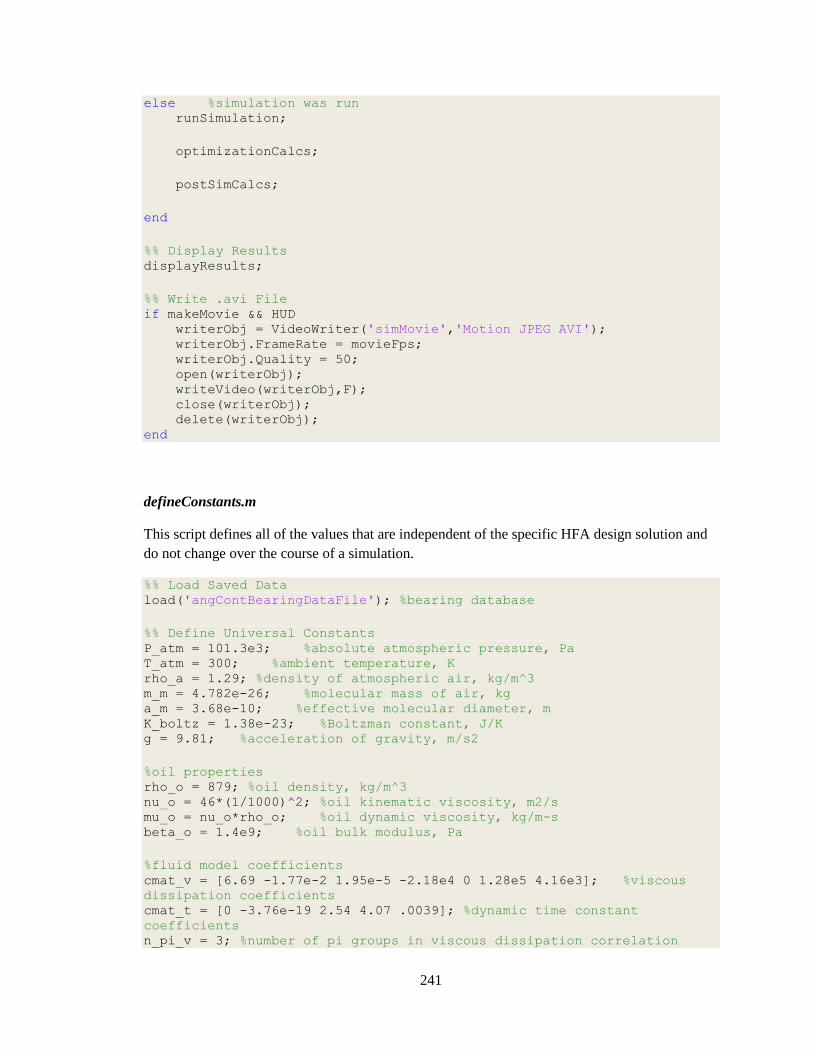
241

else %simulation was run runSimulation;

optimizationCalcs;

postSimCalcs;

end

%% Display Results displayResults;

%% Write .avi File if makeMovie && HUD writerObj = VideoWriter('simMovie','Motion JPEG AVI'); writerObj.FrameRate = movieFps; writerObj.Quality = 50; open(writerObj); writeVideo(writerObj,F); close(writerObj); delete(writerObj); end

defineConstants.m

This script defines all of the values that are independent of the specific HFA design solution and

do not change over the course of a simulation.

%% Load Saved Data load('angContBearingDataFile'); %bearing database

%% Define Universal Constants P_atm = 101.3e3; %absolute atmospheric pressure, Pa T_atm = 300; %ambient temperature, K rho_a = 1.29; %density of atmospheric air, kg/m^3 m_m = 4.782e-26; %molecular mass of air, kg a_m = 3.68e-10; %effective molecular diameter, m K_boltz = 1.38e-23; %Boltzman constant, J/K g = 9.81; %acceleration of gravity, m/s2

%oil properties rho_o = 879; %oil density, kg/m^3 nu_o = 46*(1/1000)^2; %oil kinematic viscosity, m2/s mu_o = nu_o*rho_o; %oil dynamic viscosity, kg/m-s beta_o = 1.4e9; %oil bulk modulus, Pa

%fluid model coefficients cmat_v = [6.69 -1.77e-2 1.95e-5 -2.18e4 0 1.28e5 4.16e3]; %viscous

dissipation coefficients cmat_t = [0 -3.76e-19 2.54 4.07 .0039]; %dynamic time constant

coefficients n_pi_v = 3; %number of pi groups in viscous dissipation correlation

242

order_v = 3; %order of polynomial fit for viscous dissipation

correlation n_pi_t = 3; %number of pi groups in dynamic time constant correlation order_t = 2; %order of polynomial fit for dynamic time constant

correlation

%% Define Vehicle Specs %vehicle external characteristics f_af = 0.08; %frontal area factor f_m = 0.04; %mass factor C_d = 0.3; %drag coefficient A_f = f_af*2.3; %frontal area, m2 m_v = f_m*1800; %mass, kg a_1 = .009; %basic rolling coefficient a_2 = .0035; %speed rolling coefficient eta_trans = 1; %transmission efficiency d_t = .664; %tire diameter (P215/60R16 94V), m

%% Define Control and Drive Cycle Specs %control strategy parameters P_d = 3000*(101300/14.7) + P_atm; %desired hydraulic system pressure,

Pa t_switchMin = .5; %minimum time between switching power methods f_control = .06; %control band (full range), fraction of desired

system pressure R_control = 1.5; %PM sizing goal for f_pressure/f_control utilVDPM_min = 0.95; %minimum required VDPM utilization

%select number of drive cycle "laps" and time step size N_dc = 1; %number of laps dt = 0.125; %time step size

%laboratory specifications W_dot_lab = 3000*(101300/14.7)*5*0.000063; %hydraulic power supply

capacity, W

%% Define Maximum Expected Loading T_max = 200; %guess for the maximum expected torque, N-m G = 6.3; %balancing grade (ISO 1943), mm/s SF_ecc = 10; %safety factor on eccentricity, used for bearing selection

%% Define Accumulator Materials and Architecture arch = [1 1 1]; %architecture definition array, [0=outside/1=inside;

0=VD/1=FD; 0=metal/1=composite-wrapped] SF = 3; %safety factor for material failure

%housing switch arch(3) case 0 [rho_h, nu_h, E_h, S_y_h] = propsMetal('ti');

case 1 %composite [rho_c, E1, E2, nu12, nu21, X, Y, Yc] =

propsComposite('T300/2500');

243

%liner [rho_l, nu_l, E_l, S_y_l] = propsMetal('4140_q_t205_1in'); end

%end caps [rho_e, nu_e, E_e, S_y_e] = propsMetal('7075');

%axle (bolt) [rho_b, nu_b, E_b, S_y_b] = propsMetal('4340_q800_t540_4in');

%piston [rho_p, nu_p, E_p, S_y_p] = propsMetal('7075'); BR = 1.5; %piston-tie rod bearing ratio

%chamber [rho_ch, nu_ch, E_ch, S_y_ch] = propsMetal('4140');

%% Define Axle and End Cap Constants N_p = 1; %number of radial ports f_p_i = 1; %port diameter fraction k_exit = 1; %pipe exit loss coefficient k_entr = .4; %pipe entrance loss coefficient k_tee = .3; %tee loss coefficient epsilon = 1.6*(1e-6); %surface roughness, smooth turned, micron mu_st_st = .5; %steel-on-steel friction coefficient (conservative) mu_st_al = .61; %steel-on-aluminum friction coefficient d_lp = .01; %leakage port diameter, m gap = .002; %HSRU safety gap, m

%% Define Bearing constants C_b_m = 1.0e-3; %bearing torque mass coefficient, Nm/kg N_b = 2; %number of bearings

%% Define Containment Chamber and Feedthrough Parameters c_ch = 0.01; %chamber-HFA clearance, m N_ring = 2; %number of o-rings required to seal containment chamber

if arch(1) == 0 P_ch_d = .1; %desired chamber pressure, Pa Q_ft = 1e-11*(101300/1)*(1/100)^3; %FerroTec shaft seal leakage

rate (conv. from Std ccHe/s), Pa-m3/s C_ft_c = 0.0148; %feedthrough drag torque constant, Nm C_ft_s = 9e-5; %feedthrough drag torque slope coefficient,

Nm/rad/s else P_ch_d = 14; %desired chamber pressure (higher than P_vap for

oil), Pa Q_ft = 0; %no rotary shaft seal C_ft_c = 0; %no feedthrough C_ft_s = 0; %no feedthrough end f_band_vac = .005; %allowable fraction above desired pressure beta_ch = 1.4; %ratio of spec heats (air) S_p_on = 1e-4; %pumping speed, m3/s

244

%% Define HFA Pump/Motor Specs G_PM = 1; %pump-motor gear ratio eta_GR = 1; %gear reduction efficiency a_spd = 32.04; %a-coefficient for D-omega_max correlation b_spd = -0.2812; %b-coefficient for D-omega_max correlation m_mass = 2.36e5; %m-coefficient for D-mass correlation b_mass = 1.123; %b-cofficient for D-mass correlation len_PM = .25; %approximate length of PM (as well as shafts and HSRU

case), m

%manufacturer loss coefficients C_s = 4.259e-9; %laminar slip coefficient C_st = 0; %turbulent slip coefficient C_v = 23523; %viscous loss coefficient C_f = .0537; %frictional loss coefficient C_h = 53.56; %hydrodynamic loss coefficient

propsMetal.m

This function stores various material properties for the metals used in the HFA.

function [rho, nu, E, S_y] = propsMetal(matl) %rho: material density, kg/m3 %nu: Poisson Ratio

%E: Young's Modulus, Pa %S_y: tensile yield strength, Pa switch matl % Steels case '4140' %AISI 4140 alloy steel (azom.com) rho = 7850; nu = .3; E = 200e9; S_y = 415e6; case '4340_q800_t540_4in' %AISI 4340, oil quenched 800C, 540

temper (matweb) rho = 7850; nu = .29; E = 205e9; S_y = 1000e6; S_y = 1515e6;

% Aluminums case '7075' %7075-T6 aluminum (asm.matweb.com) rho = 2810; nu = .33; E = 72e9; S_y = 503e6; case 'gray iron' rho = 7150; nu = .29; E = 110e9; S_y = 290e6; end

245

propsComposite.m

This function is the composite material counterpart to the function propsMetal.m (above).

Though the material T300/#2500 was the only composite used for the present research, several

others are stored in this function to facilitate material tradeoff studies.

function [rho, E1, E2, nu12, nu21, X, Y, Yc] = propsComposite(matl) %rho: composite density, kg/m3 %t: ply thickness, m %E1: fiber-direction Young's Modulus, Pa %E2: transverse Young's Modulus, Pa %G12: shear modulus, Pa %nu12: 1-2 Poisson's ratio (strain in 1-direction causing strain in 2-

direction) %nu21: 2-1 Poisson's ratio %X: tensile strength in fiber direction, Pa %Y: tensile strength perpendicular to fiber direction, Pa %Yc: compressive strength perpendicular to fiber direction, Pa switch matl case 'HM' %HM Graphite/Epoxy (??) rho = 1.63e3; E1 = 230e9; E2 = 6.6e9; nu12 = .25; nu21 = nu12*E2/E1; X = 1100e6; Y = 21e6; Yc = 100e6; case 'T300/2500' %T300 Carbon Fiber, 2500 Epoxy (Ha) rho = 1600; E1 = 130e9; E2 = 9e9; nu12 = .3; nu21 = nu12*E2/E1; X = 1800e6; Y = 80e6; Yc = 168e6; case 'T300/BSL914C' %T300 Carbon Fiber, CSL914C Epoxy (Soden)

(V_f=0.6) rho = 1600; E1 = 138e9; E2 = 11e9; nu12 = .28; nu21 = nu12*E2/E1; X = 1500e6; Y = 27e6; Yc = 200e6; end

246

driveCycleSetup.m

This script imports the EPA-specified UDDS from a text file in the working directory called

‘uddscol.txt,’ increases the drive cycle resolution, and calculates various drive cycle

characteristics that are independent of the specific HFA design solution.

%import and duplicate drive cycle driveCycle = importdata('uddscol.txt'); %import drive cycle dt_unr = driveCycle(2,1) - driveCycle(1,1); %unresolved time step size,

s v_mph = []; %build vehicle velocity array, mph for i = 1:N_dc v_mph = vertcat(v_mph,driveCycle(:,2)); end v_unr = v_mph*1609.344/3600; %vehicle velocity, m/s

%increase drive cycle resolution [t, v, n, dt, f_time, t_tot] = increaseDCresolution(dt_unr, v_unr, dt);

%calculate other drive cycle values n = n-1; %subtract last data point because of FDE for vehicle

acceleration a = diff(v)./dt; %vehicle acceleration, m/s2 v = v(1:n); %truncated velocity array, m/s d = cumsum(v*dt); %distance array, m t = t(1:n); %truncated time array, s

loadDesignParams.m

This function extracts the design parameter values from the worskspace variable specFile

and assigns them to their appropriate variables.

function [r_o, len_i, f_th, f_l, f_d_i, l_s, c_s, omega_d, ... f_charge] = loadDesignParams(array)

%housing parameters r_o = array(1); %housing outer radius, m len_i = array(2); %HFA inner length (distance between end caps), m f_th = array(3); %fraction of housing outer radius that is material f_l = array(4); %fraction of wall material that is liner

%HSRU parameters f_d_i = array(5); %HSRU shaft inner diameter, fraction of housing

inner diameter l_s = array(6); %HSRU seal length, m c_s = array(7); %HSRU seal clearance, m

%operational parameters omega_d = array(8); %HFA maximum angular velocity, rad/s f_charge = array(9); %HFA charge pressure fraction (P_c =

f_charge*P_s)

247

end

preSimCalcs.m

This is a major script that executes all of the calculations that can or must be performed before a

drive cycle simulation. This includes most of the stress-driven dimension selections covered in

Chapter 3, as well as mass, inertia, energy capacity and road load calculations. The script also

performs a geometric feasibility check and sizes the storage PM.

%% Calculate Housing Properties th = f_th*r_o; %total wall thickness, m r_i = r_o - th; %housing inner radius, m

if arch(3) == 1 th_l = f_l*(r_o - r_i); %liner thickness, m th_c = th - th_l; %composite thickness, m r_l = r_i + th_l; %radius of liner-composite interface, m end

%% Calculate Relevant Pressures P_c = f_charge*P_d; %charge pressure, Pa rho_g_c = rho_a*P_c/P_atm; %gas density at charge (assume air

properties), kg/m3 P_s_min = (1 - f_control/2)*P_d; %upper bound on control band, Pa P_s_max = (1 + f_control/2)*P_d; %upper bound of control band, Pa P_int_max = P_s_max + (1/2)*rho_o*omega_d^2*r_i^2; %wall pressure at

max pressure condition, Pa

%% Size the Axle d_i = f_d_i*2*r_i; %HSRU shaft inner radius, m d_p = f_p_i*d_i; %port diameter, m d_s = calcSealDiameter(1.2*P_s_max,d_i,S_y_b/SF); %clearance seal

diameter, m

[r_a, P_h_max, F_b_max, F_s_max, ~, k_s, delta_a] = sizeAxle(d_i, d_s,

... r_i, len_i, N_p, d_p, S_y_b/SF, E_b, rho_o, omega_d, 1.2*P_s_max,

... rho_l*pi*len_i*(r_l^2 - r_i^2)+rho_c*pi*len_i*(r_o^2 - r_l^2), g);

%axle outer radius, m P_h_d = P_d + (1/4)*rho_o*omega_d^2*(r_i^2 + r_a^2); %design pneumatic

pressure pressure, Pa detailAxle; %perform detailed design on the axle

%% Size the End Caps P_b_max = P_s_max + (1/2)*rho_o*omega_d^2*r_a^2; %pressure at bolt

at max pressure condition, Pa %calculate required end cap length, m [len_e,P_o_worst,P_g_worst,F_b_max_check,sigma_vm_e_check] =

sizeEndCaps(r_i, r_a, r_r_o-r_a, 50, ... %geometry

248

1.2*P_s_max, omega_d, ... %worst-case parameters rho_o, rho_a, P_atm, ... %constants rho_e, E_e, nu_e, S_y_e/SF); %material properties len_h = len_i + 2*len_e; %housing length, m disp_b = F_b_max/E_b*(4*len_e/(pi*((2*r_a)^2 - d_i^2)) + ... d_p/(pi*((2*r_a)^2 - d_i^2)/4 - N_p*d_p*r_a) + ... 4*(len_i - d_p + len_e)/(pi*(2*r_a)^2)); %maximum axial

elongation of axle, m

%% Calculate Piston Dimensions th_p = sizePiston(r_i,r_a,0,P_o_worst-P_g_worst,omega_d,... rho_p,E_p,nu_p,S_y_p/SF); %piston thickness, m H_g = .005; %approximate groove depth for piston seals, m D_g = .01; %approximate groove width for piston seals, m l_pb = H_g*(SF*P_c)/(0.58*S_y_p); %minimum thickness of boss between

seals, m th_p = max(th_p,l_pb+2*D_g); %check for seal packaging th_b = 2*H_g; %thicknes of bearing section, twice seal groove height, m len_p = BR*2*r_a; %piston bearing length Vol_g_min = pi*(r_i^2-(r_a+th_b)^2)*(len_p-th_p); %minimum gas volume

(piston dead volume), m3 Vol_o_min = 0; %minimum oil volume -- in reality will be non-zero, m3 Vol_p = pi*(r_i^2-r_a^2)*len_p - Vol_g_min; %piston volume, m3

%% Values Specific to Charge and Design Conditions Vol_i = pi*len_i*(r_i^2 - r_a^2); %housing inner volume, m3 Vol_c = Vol_i - Vol_p - Vol_o_min; %gas volume at charge, m3 Vol_g_d = Vol_c*P_c/P_h_d; %gas volume at design condition, m3 Vol_o_d = Vol_i - Vol_p - Vol_g_d; %oil volume at design condition, m3 m_o_d = rho_o*Vol_o_d; %design oil mass, kg I_o_d = (1/2)*m_o_d*(r_i^2 + r_a^2); %design oil moment of

inertia, kg-m^2

%% Size the Bearings and Shafts %calculate primary mass contributions switch arch(3) case 0 m_h = rho_h*pi*len_h*(r_o^2 - r_i^2); %housing mass, kg I_h = (1/2)*m_h*(r_o^2 + r_i^2); %housing inertia, kg case 1 m_l = rho_l*pi*len_h*(r_l^2 - r_i^2); %liner mass, kg m_c = rho_c*pi*len_h*(r_o^2 - r_l^2); %composite mass, kg m_h = m_l + m_c; %housing mass, kg I_l = (1/2)*m_l*(r_l^2 + r_i^2); %liner moment of inertia,

kg-m^2 I_c = (1/2)*m_c*(r_o^2 + r_l^2); %composite moment of

inertia, kg-m^2 I_h = I_l + I_c; %housing inertia, kg-m^2 end m_e = rho_e*pi*len_e*(r_i^2 - r_a^2); %single end cap mass, kg m_b = rho_b*pi*(len_i + 2*len_e + 2*l_sh)*r_a^2; %approximate axle

mass, kg m_p = rho_p*Vol_p; %piston mass, kg m = m_h + 2*m_e + m_b + m_p; %total HFA mass so far -- excludes oil

mass, kg

249

%calculate remainder of primary inertia contributions I_e = (1/2)*m_e*(r_i^2 + r_a^2); %single end cap moment of inertia,

kg-m^2 I_b = (1/2)*m_b*r_a^2; %bolt moment of inertia, kg-m^2 I_p = (1/2)*m_p*(r_i^2 + r_a^2); %piston moment of inertia, kg-m^2 I_s = I_h + 2*I_e + I_b + I_p; %inertia of solid components, kg-m^2

%calculate radial and axial forces r_ecc_lo = G/omega_d*10^-3; %low estimate of eccentricity (based on

balance grade), m r_ecc_hi = r_ecc_lo*SF_ecc; %high estimate of eccentricity (based on

safety factor), m F_r = m*omega_d^2*r_ecc_hi; %maximum expected radial load (total), N F_a = max(F_s_max, m*g); %maximum expected axial load, N

%select bearings [d_b_i, d_b_o, w_br, ~, r_f, ~, L_nah, bearingSelected] = ... sizeBearing(d_i, F_a, F_r, 1.2*P_s_max, f_m*T_max,... S_y_b/SF, omega_d, angContBearingData, eCorr); %execute bearing

sizer function if ~bearingSelected disp('WARNING: Bearings not properly sized') end

len_pipe = len_e + l_r + l_sh + w_br + d_lp + l_s; %approximate length

of axial port, m

%% Containment Chamber R_ch_i = r_o + c_ch; %inner radius of containment chamber, m Q = calcGasLoad(R_ch_i,P_atm,N_ring); %gas load due to permeation,

Pa-m3/s Vol_ch = pi*R_ch_i^2*(len_h + 2*c_ch + len_PM) - pi*r_o^2*len_h;

%approximate chamber air volume, m3 [mu_ch, Kn] = calcChamberGas(P_ch_d/P_atm*rho_a,T_atm,len_h); %dynamic

viscosity, kg/m-s; and Knudsen number Vol_leakage_max = pi*R_ch_i^2*.05; %maximum allowable leakage into

containment chamber, approx, m3

%% Energy Capacities at Design Condition e_k_d = (1/2)*(I_s + I_o_d)*omega_d^2; %kinetic energy capacity, J e_h_d = P_c*Vol_c*log(P_h_d/P_c); %hydraulic energy capacity, J e_d = e_k_d + e_h_d; %total energy capacity, J

%% Tractive Power Profile F_aero = (1/2)*C_d*A_f*rho_a*v.^2; %vehicle aero drag, N F_roll = (m_v + m)*9.81*(a_1 + 3.24*a_2.*(v./44.7).^2.5); %vehicle

rolling drag, N F_acc = (m_v + m)*a; %force contributing to

acceleration/deceleration, N F = F_acc + F_aero + F_roll; %total force, N W_dot_t = F.*v; %tractive power, W f_power = W_dot_lab/abs(min(W_dot_t)); %ratio of laboratory HPU power

capacity to required motoring power W_dc_min = trapz(t,W_dot_t); %minimum capacity to feasibly complete

drive cycle, J

250

%% PM Initial Sizing omega_PM_max = G_PM*omega_d; %maximum HFA PM angular velocity, rad/s D_max = 2*pi*max(abs(W_dot_t))/(P_s_min*omega_PM_max); %initial

selection of storage PM displacement, m3/rev m_PM = m_mass*D_max + b_mass; %HFA PM mass omega_ax = v/(d_t/2); %axle speed

%% Geometric Feasibility Check geoInfeas = [Vol_c<0 ... %negative charge volume Vol_g_d<Vol_g_min ... %piston bearing length prevents achieving

design pressure len_i<len_p ... %piston bearing length exceeds inner length (r_i-r_a)<th_b]; %piston bearing thickness is larger than

the space between the axle and liner

calcSealDiameter.m

This function calculates the required seal diameter, 𝑑𝑠, to avoid failures of the portion of the axle

which forms the circumferential seal of the HSRU. This is done by initially guessing a very thin

wall and incrementing by small values until the von Mises stress is acceptably low. See Section

3.2 for a detailed explanation of this logic.

function d_s = calcSealDiameter(P_i,d_i,sigma_vm_d)

incr = .0001; %guessing increment, m sigma_vm = inf(1,2); %create variable to store von Mises stress at

inner and outer radii diff = inf; %fractional difference between acceptable and actual stress incrCt = 0; %iteration counter

d_s = d_i + incr; %initial guess for outer radius, m

while diff > .01 && incrCt < 1000

F = -P_i*pi/4*(d_s^2 - d_i^2); %axial compressive force

%calculate stress at inside of hollow shaft [sigma_vm(1), ~, ~, ~, ~] = ... calcShaftStress(d_i/2,F,0,0,P_i,0,0,d_i,d_s,0,0,1,1,1);

%calculate stress at outside of hollow shaft [sigma_vm(2), ~, ~, ~, ~] = ... calcShaftStress(d_s/2,F,0,0,P_i,0,0,d_i,d_s,0,0,1,1,1);

diff = (max(sigma_vm) - sigma_vm_d)/sigma_vm_d; %calculate fraction

difference in stress

if diff > 0 %stress is too high d_s = d_s + incr; %make diameter larger

251

end

incrCt = incrCt + 1; %increment iteration counter end

end

calcShaftStress.m

This function can be used to calculate the von Mises stress at a radial location 𝑟 for a generic

hollow or solid shaft. The shaft is presumed to have no end effects and can be loaded with any

combination of an axial force, bending moment, shear force, internal pressure, external pressure,

and torque.

function [sigma_vm, sigma_c, sigma_r, sigma_z, tau_rc] = ... calcShaftStress(r,F,M,V,P_i,P_o,T,d_i,d_o,d_p,N,k_n,k_b,k_t) %Loads %F -- loading (positive in tension) normal to the z-axis, N %M -- bending moment about the r (or c, equivalently) axis, N-m %V -- shear force %P_i -- presure inside (if hollow), Pa %P_o -- pressure outside, Pa %T -- torque about the z-axis, N-m

%Dimensions %d_i -- inner diameter, m %d_o -- outer diameter, m %d_p -- diameter of radial passages %N -- number of radial passages

%Stress Concentration Factors %k_n -- normal axial loading %k_b -- bending axial loading %k_t -- torsional loading

%All stresses are given in Pa. Note that the user is responsible for %specifying the correct stress concentration factor, and that only one

%is applied in a given calculation. If, for example, stress is being %calculated at a point on a shaft where radial passages coincide with a %fillet, the user should calculate a stress concentration factor for

%normal loading as

%k_n = k_n_passage*k_n_fillet

%and pass that single value to the function as k_n.

%% Calculate Shaft Properties d = 2*r; %diameter of radial point of interest, m

252

A = pi/4*(d_o^2 - d_i^2) - N*d_p*(d_o - d_i); %cross-sectional area

(normal to z-axis), m2 I = pi/64*(d_o^4 - d_i^4); %area moment of inertia, m4 J = pi/32*(d_o^4 - d_i^4); %polar area moment of inertia, m4

%% Calculate Radial Stress %The pressure differential across the shaft wall is assumed to be the

only %contributor to radial stress. The mass that the shaft supports would,

in %reality, cause some compressive radial stress, but is neglected here. %Centrifugal effects are also neglected, as the shaft diameter is

generally %small and the pressure differential large. sigma_r = (d_i^2*P_i - d_o^2*P_o)/(d_o^2 - d_i^2) ... - (P_i - P_o)*d_i^2*d_o^2/((d_o^2 - d_i^2)*d^2);

%% Calculate Circumferential Stress %The pressure differential across the shaft wall is assumed to be the

only %contributor to circumferential stress. As in the radial stress %calculation, centrifugal effects are neglected, as the shaft diameter

is %generally small and the pressure differential large. sigma_c = (d_i^2*P_i - d_o^2*P_o)/(d_o^2 - d_i^2) ... + (P_i - P_o)*d_i^2*d_o^2/((d_o^2 - d_i^2)*d^2);

%% Calculate Axial Stress %Both bending and normal loading are taken into account for bending

stress %calculation. Stress concentration factors are applied.

sigma_z_b = k_b*M*r/I; %maximum axial stress due to bending

sigma_z_n = k_n*F/A; %axial stress due to normal loading

sigma_z = sigma_z_b + sigma_z_n; %total axial stress

%% Calculate Shear Stresses tau_T = k_t*T*r/J; %torsional shear stress

if sigma_z_b == 0 tau_V = (4/3)*V/A; %maximum transverse shear stress else tau_V = 0; %shear stress is zero at the critical point end

tau_rc = tau_T + tau_V; %total shear stress

%% Calculate von Mises Stress sigma_vm = sqrt(0.5*((sigma_r - sigma_c)^2 + (sigma_c - sigma_z)^2 +

... (sigma_z - sigma_r)^2 + 6*tau_rc^2));

end

253

sizeAxle.m

This function carries out the process by which the various axle dimensions are selected, as

described in Section 3.2.

function [r_a, P_h, F_a, F_s, F_b, k_s, delta_a] = sizeAxle(d_i, d_s,

... r_i, len_i, N_p, d_p, sigma_max, E_b, rho_o, omega, P_s, m_h, g)

%coefficients for stress concentration correlation (Juvinall and

Marshek) c_n_1 = 3.2381; c_n_2 = -3.0857; c_n_3 = 2.9908;

F_p = P_s*pi*d_s^2/4; %force acting on face of axle, N

x_o = 0; %zero preload

k_s0 = 10^7; %initial guess for spring constant e = inf; %set initial error to infinity epsilon = 1e-6; %convergence criterion iterCt = 0; %iteration counter

while e >= epsilon && iterCt < 10^3;

%solve for axle radius, m r_a = fzero(@(r_a) ((P_s +

(1/4)*rho_o*omega^2*(r_i^2+r_a^2))*pi*(r_i^2-r_a^2) ... - k_s0*x_o - m_h*g)/(1 + k_s0*len_i/(pi*r_a^2*E_b)) - ... ... sigma_max*(pi*(r_a^2 - d_i^2/4)-N_p*d_p*(2*r_a-d_i))...

/(c_n_1*min(d_p/(2*r_a),3.5)^2+c_n_2*min(d_p/(2*r_a),3.5)+c_n_3)... ... ,.05);

%calculate new spring constant F_h = (P_s + (1/4)*rho_o*omega^2*(r_i^2+r_a^2))*pi*(r_i^2-r_a^2);

%hydraulic force, N F_a = (F_h - k_s0*x_o - m_h*g)/(1 + k_s0*len_i/(pi*r_a^2*E_b));

%axle force, N k_s = pi*r_a^2*E_b/(len_i*F_a)*(P_s*pi*d_s^2/4 - m_h*g); %spring

constant, N/m

%iteration operations e = abs(k_s-k_s0)/k_s; %error k_s0 = k_s; %set new guess for spring constant iterCt = iterCt + 1; %increment iteration counter end

%calculate other relevant values sigma_a = F_a/(pi*r_a^2); %average axial stress in axle, Pa delta_a = len_i*sigma_a/E_b; %axial elongation of axle, m

254

F_s = k_s0*(x_o + delta_a); %spring force, N F_b = F_s + m_h*g - F_p; %reaction force at bottom bearing (should

be zero), N P_h = P_s + (1/4)*rho_o*omega^2*(r_i^2+r_a^2); %hydraulic pressure,

Pa

end

sizeEndCaps.m

This function calculates the required end cap thickness based on the centrifugal and pressure

loading on the end caps. The gas and oil side end caps are evaluated separately, using their

respective pressure distributions. The end cap that experiences more bending dictates the

required end cap length, per the discussion in Section 3.3.

function [len_e, P_o, P_g, F_g_max, sigma_vm_max] = ... sizeEndCaps(r_i, r_a, dp, nr, ... P_s, omega, rho_o, rho_atm, P_atm, rho_e, E_e, nu_e, sigma_max)

r = linspace(r_a,r_i,nr); %radial position vector, m

%% Calculate Centrifugal Stresses [~, sigma_r_cent, sigma_c_cent, ~] = calcStressIso(r_a, r_i, nr, ... omega, 0, 0, 0, rho_e, E_e, nu_e);

%% Calculate Bending Moments free = 1; %free support at inner edge

%calculate oil-side loading P_o = P_s + (1/2)*rho_o*omega^2*r.^2; %oil-side pressure distn, Pa

%calculate gas-side loading P_avg = P_s + (1/4)*rho_o*omega^2*(r_i^2 + r_a^2); %average

pressure, Pa A_p = pi*(r_i^2-r_a^2); %area of piston face, m2 Cg0 = rho_atm/P_atm; %constant 0, used for gas pressure profile Cg1 = Cg0*omega^2/2; %constant 1, used for gas pressure profile Cg2 = P_avg*A_p/(2*pi); %constant 2, used for gas pressure profile P_g0 = 2*Cg1*Cg2/(exp(Cg1*r_i^2) - exp(Cg1*r_a^2)); %gas pressure at

radial center P_g = exp(Cg0*omega^2*r.^2/2 + log(P_g0)); %gas pressure distribution,

Pa

%calculate oil side end cap bending moments [M_t_o, M_r_o, F_g_max, ~] = bendingHeap(r_i, r_a, dp, free, ... P_o, nu_e);

%calculate gas side end cap bending moments [M_t_g, M_r_g, ~, ~] = bendingHeap(r_i, r_a, dp, free, ... P_g, nu_e); %end cap length required on gas side, m

255

%% Find Required Thickness incr = 0.0001; %sizing increment, m maxLen = .2; %maximum reasonable end cap length, m sized = 0; %default to not yet properly sized len_e = 0; %initial guess for end cap length, m

%cycle through end cap sizes while ~sized && (len_e < maxLen)

len_e = len_e + incr; %incrememnt end cap length

%check oil side sigma_r = sigma_r_cent + 6*M_t_o/len_e^2; %total radial stress

distn, Pa sigma_c = sigma_c_cent + 6*M_r_o/len_e^2; %total circumferential

stress distn, Pa sigma_vm = sqrt(sigma_r.^2 - sigma_r.*sigma_c + sigma_c.^2);

%von Mises stress distn, Pa

if max(sigma_vm) <= sigma_max %if oil side passes, check gas side

sigma_r = sigma_r_cent + 6*M_t_g/len_e^2; %total radial stress

distn, Pa sigma_c = sigma_c_cent + 6*M_r_g/len_e^2; %total

circumferential stress distn, Pa sigma_vm = sqrt(sigma_r.^2 - sigma_r.*sigma_c + sigma_c.^2);


if max(sigma_vm) <= sigma_max %check to see if stress is

acceptably low sized = 1; end

end

end

sigma_vm_max = max(sigma_vm); %get maximum von Mises stress value

end

calcStressIso.m

This function calculates the stresses and radial strain due to internal pressure, external pressure

and centrifugal forces in an isotropic solid or hollow cylinder. Methods used are presented by

Genta [25].

function [r, sigma_r, sigma_c, u_r] = calcStressIso(r_i, r_o, nr,

omega, ...

256

P_int, P_ext, sigma_z, rho, E, nu)

beta = r_i/r_o; %calculate radius ratio X = linspace(beta,1,nr); %create dimensionless radial position

vector

if beta==0 %solid

%radial stress, Pa sigma_r_cent = rho*omega^2*r_o^2*(3+nu)/8*(1 - X.^2); %centrifugal

component sigma_r_ext = -P_ext; %external pressure component sigma_r = sigma_r_cent + sigma_r_ext; %total

%circumferential stress, Pa sigma_c_cent = rho*omega^2*r_o^2*(3+nu)/8*(1 -

(1+3*nu)/(3+nu)*X.^2); %centrifugal component sigma_c_ext = -P_ext; %external pressure component sigma_c = sigma_c_cent + sigma_c_ext; %total

else %central hole

%radial stress, Pa sigma_r_cent = rho*omega^2*r_o^2*(3+nu)/8*(1 + beta^2 - ... beta^2./X.^2 - X.^2); %centrifugal component sigma_r_int = -P_int*beta^2/(1 - beta^2)*(1/beta^2 - 1);

%internal pressure component sigma_r_ext = -P_ext/(1 - beta^2)*(1 - beta^2./X.^2); %external

pressure component sigma_r = sigma_r_cent + sigma_r_int + sigma_r_ext; %total

%circumferential stress, Pa sigma_c_cent = rho*omega^2*r_o^2*(3+nu)/8*(1 + beta^2 + ... beta^2./X.^2 - (1+3*nu)/(3+nu)*X.^2); %centrifugal component sigma_c_int = P_int*beta^2/(1 - beta^2)*(1/beta^2 + 1); %internal

pressure component sigma_c_ext = -P_ext/(1 - beta^2)*(1 + beta^2./X.^2); %external

pressure component sigma_c = sigma_c_cent + sigma_c_int + sigma_c_ext; %total

end

%calculate displacement r = r_o*X; %radial position vector, m epsilon_c = 1/E*(sigma_c - nu*(sigma_r + sigma_z)); %circumferential

strain, m/m u_r = r.*epsilon_c; %radial displacement, m

end

257

bendingHeap.m

This function uses methods presented by Heap [31], as described in Section 3.3, to calculate the

radial distribution of bending moments in component that can be approximated as a circular plate.

function [M_t, M_r, F_b, r] = bendingHeap(a, b, dp, bFree, P_net, nu)

dp = min(dp,a-b); %limit retainer contact area nr = length(P_net); %radial spatial resolution r = linspace(b,a,nr); %radial position vector dr = r(2)-r(1); %radial step size, m rsq = r.^2; %vectorized square of radial position vector A = 2*pi*r*dr; %area of each numerical discretization, m2 np = round(dp/dr); %number of discrete steps across which the reaction

force spans

%calculate net pressure and force distn F_net = P_net.*A; %net force distn F_b = sum(F_net); %axle reaction force F_net(1:np) = F_net(1:np) - F_b/np; %net line load distribution, N

%create moment arrays M_r = zeros(1,nr); %radial moment distribution, Nm/m M_t = zeros(1,nr); %tangential moment distribution, Nm/m

if bFree %inner edge free (Heap load case VIII)

%calculate constants for efficiency %interior moments C0_i = (1/2)*(1-nu)/(1+nu); Cr_i = 1/(4*pi)*(1+nu)*(1-b^2./rsq)*(a^2/(a^2-b^2)); Ct_i = 1/(4*pi)*(1+nu)*(1+b^2./rsq)*(a^2/(a^2-b^2)); %exterior moments C0_o = 1/(4*pi)*(1+nu)*(a^2/(a^2-b^2)); Cr_o1 = (1/2)*(1-nu)/(1+nu)*(1 - rsq/a^2); Cr_o2 = log(a./r); Ct_o1 = (1/2)*(1-nu)/(1+nu)*(1+a^2./rsq); Ct_o2 = (1/2)*(1-nu)/(1+nu)*(1-rsq/a^2)*(a^2-b^2)./rsq; Ct_o3 = log(a./r);

for j=1:nr %cycle through line loads d = r(j); %get postiion of line load

%calculate bending moments interior to line load M_r(1:j) = M_r(1:j) + F_net(j)*Cr_i(1:j)*(C0_i*(1-d^2/a^2) +

log(a/d)); M_t(1:j) = M_t(1:j) + F_net(j)*Ct_i(1:j)*(C0_i*(1-d^2/a^2) +

log(a/d));

%calculate bending moments exterior to line load M_r(j+1:nr) = M_r(j+1:nr) + F_net(j)*C0_o*(Cr_o1(j+1:nr)*(d^2-

b^2)./rsq(j+1:nr) ...

258

+ Cr_o2(j+1:nr) + b^2/a^2*log(r(j+1:nr)/d) -

b^2./rsq(j+1:nr)*log(a/d)); M_t(j+1:nr) = M_t(j+1:nr) + F_net(j)*C0_o*(Ct_o1(j+1:nr)*(1 -

d^2/a^2) ... - Ct_o2(j+1:nr) + Ct_o3(j+1:nr) + b^2/a^2*log(r(j+1:nr)/d)

+ b^2./rsq(j+1:nr)*log(a/d));

end

else %moment reaction at inner edge (Heap load case IX)

%calculate constants for efficiency C0 = (1+nu)/(1-nu); %interior moments Cr_i = 1/(4*pi)*(1-nu)*(C0 + b^2./rsq)/(C0 + b^2/a^2); Ct_i = 1/(4*pi)*(1-nu)*(C0 - b^2./rsq)/(C0 + b^2/a^2); %exterior moments C_o = 1/(4*pi)*((1+nu)/(C0 + b^2/a^2)); Cr_o1 = (1/2)*(1-rsq/a^2)./rsq; Cr_o2 = Cr_o1*b^2/C0 + C0*log(a./r); Cr_o3 = b^2./rsq; Cr_o4 = b^2/a^2; Ct_o2 = Cr_o3; Ct_o3 = Cr_o4; Ct_o1 = (1/2)*(Ct_o3 - Ct_o2)/C0; for j=1:nr %cycle through line loads d = r(j); %get postiion of line load

%calculate bending moments interior to line load M_r(1:j) = M_r(1:j) + F_net(j)*Cr_i(1:j)*((1-d^2/a^2)/2 +

C0*log(a/d)); M_t(1:j) = M_t(1:j) + F_net(j)*Ct_i(1:j)*((1-d^2/a^2)/2 +

C0*log(a/d));

%calculate bending moments exterior to line load M_r(j+1:nr) = M_r(j+1:nr) + F_net(j)*C_o*(Cr_o1(j+1:nr)*d^2 +

... Cr_o2(j+1:nr) + Cr_o3(j+1:nr)*log(a/d) -

Cr_o4.*log(r(j+1:nr)./d)); M_t(j+1:nr) = M_t(j+1:nr) + F_net(j)*C_o*(1 ... - (d^2/a^2 + d^2./rsq(j+1:nr))/2 + Ct_o1(j+1:nr) ... - Ct_o2(j+1:nr)*log(a/d) - Ct_o3*log(r(j+1:nr)/d));

end

end

end

259

sizePiston.m

This function uses the methods described in Section 3.4 to properly select the piston thickness.

function th_p =

sizePiston(r_i,r_a,dp,P_net,omega,rho_p,E_p,nu_p,sigma_max)

%% Calculate Centrifugal Stresses [~, sigma_r_cent, sigma_c_cent, ~] = calcStressIso(r_a, r_i,

length(P_net), ... omega, 0, 0, 0, rho_p, E_p, nu_p);

%% Calculate Bending Moments free = 0; %moment reaction at inner edge

%calculate oil side end cap bending moments [M_t, M_r, ~, ~] = bendingHeap(r_i, r_a, dp, free, ... P_net, nu_p);

%% Find Required Thickness incr = 0.0001; %sizing increment, m maxTh = .2; %maximum reasonable end cap length, m sized = 0; %default to not yet properly sized th_p = 0; %initial guess for end cap length, m

while ~sized && (th_p < maxTh)

th_p = th_p + incr; %incrememnt end cap length

%calculate stresses sigma_r = sigma_r_cent + 6*M_t/th_p^2; %total radial stress distn,

Pa sigma_c = sigma_c_cent + 6*M_r/th_p^2; %total circumferential

stress distn, Pa sigma_vm = sqrt(sigma_r.^2 - sigma_r.*sigma_c + sigma_c.^2);


sized = max(sigma_vm) <= sigma_max; %check for proper sizing

end

end

sizeBearing.m

This function uses the logic present in Section 3.6 to properly select the bearings.

function [d, D, B, P, r_f, omega_max, L_nah, selected] = ... sizeBearing(d_i, F_a, F_r, P_i, T,...

260

sigma_max, omega_min, angContBearingData, eCorr)

%% Find Minimum Bearing Inner Diameter to Prevent Failure at Axle

Shoulders br = 0; %start at beginning of bearing data sigma_vm = inf(1,3); %initialize von Mises stress array for axle

shoulders while (max(sigma_vm) >= sigma_max) && (br < size(angContBearingData,1)) br = br + 1; d = angContBearingData(br,1)/1000; %bearing inner diameter, m r_f = angContBearingData(br,6)/1000; %bearing fillet radius, m roverd = min(0.3,max(0.025,r_f/d)); %ratio of fillet radius to

bearing inner diameter k_n = 21.143*roverd^2 - 11.55*roverd + 3.072; %normal stress

conc. factor k_t = 0.8235*roverd^(-0.264); %torsion stress conc. factor

%oil side [sigma_vm(1), ~, ~, ~, ~] = ... calcShaftStress(d_i/2,-F_a,0,F_r,P_i,0,0,d_i,d,0,0,k_n,1,k_t);

%inside

[sigma_vm(2), ~, ~, ~, ~] = ... calcShaftStress(d/2,-F_a,0,F_r,P_i,0,0,d_i,d,0,0,k_n,1,k_t);

%outside

%gas side [sigma_vm(3), ~, ~, ~, ~] = ... calcShaftStress(d/2,0,0,F_r,0,0,T,0,d,0,0,k_n,1,k_t);

end

%% Select Smallest Allowable Bearing that Can Withstand Axial and

Radial Loads selected = 0; %default to not yet properly selected while ~selected && (br <= size(angContBearingData,1)) %cycle through

bearings

%get specs of current bearing d = angContBearingData(br,1)/1000; %bearing inner diameter, m D = angContBearingData(br,2)/1000; %bearing outer diameter, m B = angContBearingData(br,3)/1000; %bearing width, m alpha_0 = angContBearingData(br,16); %contact angle, deg C = angContBearingData(br,17); %dynamic load rating, N C_0 = angContBearingData(br,18); %static load rating, N omega_max = angContBearingData(br,19)*pi/30; %speed value, rad/s

%get X and Y factors X_0 = 0.5; if alpha_0 == 25 %25 degree contact angle Y_0 = 0.38; e = 0.68; if F_a/F_r <= e X = 1; Y = 0;

261

else X = 0.41; Y = 0.87; end else %15 degree contact angle Y_0 = 0.46; e = interp1(eCorr(:,1),eCorr(:,2),F_a/C_0,'pchip'); if F_a/F_r <= e X = 1; Y = 0; else X = 0.44; Y = interp1(eCorr(:,1),eCorr(:,3),F_a/C_0,'pchip'); end end

P = X*F_r + Y*F_a; %equivalent dynamic load, N P_0 = max(F_r,X_0*F_r + Y_0*F_a); %equivalent static load, N

if (P < C) && (omega_min < omega_max) %&& (P_0 < C_0) selected = 1; else br = br + 1; end

a1 = .62; %95% relability factor ft = 1; %150 max temp n = 30*omega_min/pi/2; %avg operating speed, 1/min L_nah = a1*ft*10^6/(60*n)*(C/P)^3; %corrected operating life, h

end

end

calcChamberGas.m

This function uses the methods presented in Section 4.4 to calculate the viscosity of the low-

pressure gas in the containment chamber.

function [mu, Kn] = calcChamberGas(rho,T,len_h)

%constants m = 4.782e-26; %molecular mass of air, kg K = 1.38e-23; %Boltzman constant, J/K a_inf = 2.96e-10; %effective molecular diameter at infinite temp, m T_c = 113; %Sutherland constant, K

%calculate Knudsen number and viscosity a = a_inf*sqrt(1 + T_c/T); %effective molecular diameter, m lambda = m/(sqrt(2)*a^2*rho*pi); %mean free path, m (4.8) Kn = lambda/len_h; %Knudsen number

262

mu = sqrt(K*m*T)/(a^2*pi^(3/2)); %dynamic viscosity, kg/m-s (4.11)

end

runSimulation.m

This script executes the drive cycle simulation, the details of which were given in Section 6.4.

The script also includes code which facilitates an iterative pump-sizing algorithm.

%% Make Initial Calculations %calculations for effiency C_1 = 1/(pi*(r_i^2 - r_a^2)); C_2 = (1/2)*rho_o*(r_i^2 + r_a^2); C_3 = (1/4)*rho_o*(r_i^2 + r_a^2); C_4 = rho_a/P_atm; C_5 = 1/G_PM; C_6 = pi*d_s*c_s^3/(12*mu_o*l_s); C_7 = beta_ch/(beta_ch-1); C_8 = (beta_ch-1)/beta_ch; C_9 = P_c*Vol_c;

sized = 0; %default to incorrectly sized PM sizeCt = 0; %counter for PM sizing iterations

%% Iterate to Find Correct PM Size while ~sized %loop while PM is not properly sized

D_max = min(max(D_max,0.01e-6),200e-6); %enforce reasonable bounds

on PM size fprintf([num2str(sizeCt+1),'. Attempting pump size

',num2str(D_max*1e6),' cc/rev\n']);

%% Initialize Arrays for Data Storage %HFA state omega_s = zeros(n,1); omega_f = zeros(n,1); P_s = zeros(n,1); P_0 = zeros(n,1); P_h = zeros(n,1); Vol_o = zeros(n,1); Vol_g = zeros(n,1); L = zeros(n,1); I_o = zeros(n,1); e_k = zeros(n,1); e_h = zeros(n,1); e_k_check = zeros(n,1); e_h_check = zeros(n,1); e_check = zeros(n,1); e_dot_k = zeros(n,1); e_dot_h = zeros(n,1); e = zeros(n,1); SOC = zeros(n,1);

263

SOC_k = zeros(n,1); SOC_h = zeros(n,1); W_dot_loss = zeros(n,1); eta_inst = zeros(n,1); P_int_o = zeros(n,1);

%control and results W_dot = zeros(n,1); D = zeros(n,1); omega_PM = zeros(n,1); x = zeros(n,1); W_dot_s = zeros(n,1); eta_m = zeros(n,1); eta_v = zeros(n,1); W_dot_k = zeros(n,1); W_dot_h = zeros(n,1); pwrMode = zeros(n,1); T = zeros(n,1);

%fluid model tau_dyn = zeros(n,1); W_dot_vi = zeros(n,1); deltaO = zeros(n,1); pi1_v = zeros(n,1); pi1_t = zeros(n,1); p_v_t = zeros(n,n_pi_v-1); p_t_t = zeros(n,n_pi_t-1);

%kinetic parameters alpha_s = zeros(n,1); alpha_f = zeros(n,1); W_dot_PM = zeros(n,1); W_dot_vh = zeros(n,1); W_dot_w = zeros(n,1); W_dot_b = zeros(n,1); W_dot_ft = zeros(n,1); Sigma_kl = zeros(n,1);

%pneumatic parameters Vol_dot_o = zeros(n,1); Vol_dot_l = zeros(n,1); dP_p = zeros(n,1); dP_c = zeros(n,1); I_dot_o = zeros(n,1); dP_main = zeros(n,1); dP_port = zeros(n,1); f_bar_main = zeros(n,1); f_bar_port = zeros(n,1); W_dot_l = zeros(n,1); W_dot_p = zeros(n,1);

%containment chamber vacuum system P_ch = zeros(n,1); P_dot_ch = zeros(n,1); rho_ch_a = zeros(n,1); vacOn = zeros(n,1);

264

W_dot_vac = zeros(n,1);

%% Initialize Values for Drive Cycle t_switchLast = -inf; %set last switch beginning Vol_leakage = 0; %total amount of oil leaked into chamber, m3

if optimizing setICs; else % simulationICs; setICs; end

%% Initialize Movie Parameters if HUD

maxSizeCt = 1; F = struct('cdata',[],'colormap',[]); frameInitialization frameUpdate F(1) = getframe(allFigs); frameNumber = 2;

end

%% Run Drive Cycle for i=2:n

%% New HFA State omega_s(i) = omega_s(i-1) + alpha_s(i-1)*dt; %container

angular velocity, rad/s omega_f(i) = omega_f(i-1) + alpha_f(i-1)*dt; %oil angular

velocity, rad/s deltaO(i) = omega_s(i) - omega_f(i); %angular velocity

difference, rad/s Vol_o(i) = Vol_o(i-1) + Vol_dot_o(i-1)*dt; %oil volume, m^3 L(i) = C_1*(Vol_o(i) - Vol_o_min); %oil length, m I_o(i) = C_2*Vol_o(i); %oil moment of inertia, kg-m^2 Vol_g(i) = Vol_g(i-1) - Vol_dot_o(i-1)*dt; %gas volume, m^3 P_h(i) = C_9/Vol_g(i); %gas pressure, Pa P_0(i) = P_h(i) - C_3*omega_f(i)*omega_f(i); %pressure at

center of oil volume, Pa P_int_o(i) = P_0(i) + (1/2)*rho_o*omega_f(i)^2*r_i^2; omega_PM(i) = C_5*omega_s(i); %PM speed after gear reduction,

rad/s

%% New HFA Energy e_k(i) = (1/2)*I_s*omega_s(i)^2 + (1/2)*I_o(i)*omega_f(i)^2;

%kinetic energy stored, J e_h(i) = C_9*log(P_h(i)/P_c); %hydraulic energy stored, J e(i) = e_k(i) + e_h(i); %total energy stored, J SOC(i) = e(i)/e_d; %SOC SOC_k(i) = e_k(i)/e_k_d; %kinetic SOC SOC_h(i) = e_h(i)/e_h_d; %hydraulic SOC

265

%% Vacuum Equations and Control P_ch(i) = P_ch(i-1) + P_dot_ch(i-1)*dt; %chamber pressure,

Pa rho_ch_a(i) = C_4*P_ch(i); %chamber air density, kg/m3 vacOn(i) = vacuumToggle(P_ch(i),P_ch_d,vacOn(i-1),f_band_vac);

%vacuum pump deadband control S_p = vacOn(i)*S_p_on; %vacuum pumping speed (on or off),

m^3/s if arch(1) == 1 Vol_ch = Vol_ch - Vol_dot_l(i-1)*dt; %account for oil

leakage end P_dot_ch(i) = (Q - P_ch(i)*S_p + P_ch(i)*Vol_dot_l(i-

1))/Vol_ch; %rate of change of chamber pressure, Pa/s W_dot_vac(i) = P_ch(i)*S_p*C_7*((P_atm/P_ch(i))^C_8 - 1);

%vacuum pumping power consumption, W

%% Control Strategy and Power Calculations W_dot(i) = pwrMgmt(W_dot_t(i), SOC(i), 1); %power into (+) or

out of (-) HFA, W

%disregard switching frequency limit if PM must switch

direction anyway if W_dot(i)*W_dot(i-1) <= 0 t_switchLast = 0; end

%call control strategy [pwrMode(i), depleted, t_switchLast] =

cfun_simpleBand(W_dot(i), ... Vol_o(i), Vol_o_min, Vol_g(i), Vol_g_min, pwrMode(i-1),

i*dt, ... t_switchLast, t_switchMin, P_s(i-1), P_s_min, P_s_max, dt);

%% Pump/motor Equations %calculate efficiencies, displacement position, shaft, and

fluid %power switch arch(2) case 0 %VDPM [eta_m(i),eta_v(i),x(i),W_dot_k(i),W_dot_s(i)] = ... calcPwrVDPM(W_dot(i),pwrMode(i),P_s(i-

1),omega_PM(i),...

D_max,C_v,C_f,C_h,C_s,C_st,rho_o,mu_o,beta_o,eta_GR); case 1 %FDPM [eta_m(i),eta_v(i),x(i),W_dot_k(i),W_dot_s(i)] = ... calcPwrFDPM(W_dot(i),pwrMode(i),P_s(i-

1),omega_PM(i),...

D_max,C_v,C_f,C_h,C_s,C_st,rho_o,mu_o,beta_o,eta_GR); end W_dot_PM(i) = W_dot_k(i) - W_dot_s(i); %PM loss, W D(i) = x(i)*D_max; %instantaneous displacement, m3/rev

%% Pneumatic Equations

266

W_dot_h(i) = W_dot(i) - W_dot_k(i); %pneumatic power, W

%assign minor loss coefficients for flow through axle ports if W_dot_h(i) >=0 %pneumatic charging k_pipe = k_entr + k_tee; k_port = 2*k_exit; else %pneumatic discharging k_pipe = k_tee + k_exit; k_port = 2*k_entr; end

%calculate pressure drop due to flow through axle ports [dP_main(i), f_bar_main(i)] = calcDeltaP(Vol_dot_o(i-

1),d_i/2,len_pipe,epsilon,... k_pipe,rho_o,mu_o); %pressure drop thru axial section, Pa [dP_port(i), f_bar_port(i)] = calcDeltaP(Vol_dot_o(i-

1)/(2*N_p),d_p/2,r_a,... epsilon,k_port,rho_o,mu_o); %pressure drop thru radial

ports, Pa dP_p(i) = dP_main(i) + dP_port(i); %pressure drop through

ports, Pa

%perform remainder of pneumatic calculations P_s(i) = P_0(i) + sign(W_dot_h(i))*dP_p(i);

Vol_dot_l(i) = C_6*P_s(i); %leakage from HSRU, based on

internal pressure, m3/s Vol_leakage = Vol_leakage + Vol_dot_l(i)*dt; %increment

leaked oil volume, m3

Vol_dot_o(i) = W_dot_h(i)/P_s(i) - Vol_dot_l(i); %oil flow

rate into (+) accumulator, m3/s I_dot_o(i) = C_2*Vol_dot_o(i); %rate of change of moment of

inertia, kg-m2/s

W_dot_l(i) = Vol_dot_l(i)*P_s(i); %power loss due to leakage, W W_dot_p(i) = abs(Vol_dot_o(i)*dP_p(i)); %port loss, W

%% Dynamic Time Constant Calculation p_t_t(i,1) = L(i)^4*alpha_s(i-1)/nu_o^2; %first tau Pi group p_t_t(i,2) = alpha_s(i-1)/omega_s(i)^2; %second tau Pi

group pi1_t(i) = cmat_t(length(cmat_t)); %apply offset for j=1:n_pi_t-1 %cycle thru Pi groups for k=1:order_t %cycle thru polynomial terms pi1_t(i) = pi1_t(i) + cmat_t((j-

1)*order_t+k)*p_t_t(i,j)^k; end end tau_dyn(i) = max(0,1/(pi1_t(i)*omega_s(i))); %dynamic time

constant, s

%% Viscous Dissipation Calculation p_v_t(i,1) = sqrt(max(0,rho_o*omega_s(i)*L(i)^2/mu_o)); p_v_t(i,2) = deltaO(i)/omega_s(i);

267

pi1_v(i) = cmat_v(length(cmat_v)); %apply offset for j=1:n_pi_v-1 %cycle thru pi groups for k=1:order_v %cycle thru polynomial terms pi1_v(i) = pi1_v(i) + cmat_v((j-

1)*order_v+k)*p_v_t(i,j)^k; end end W_dot_vi(i) = max(0,mu_o*r_i^3*deltaO(i)^2*pi1_v(i));

%internal viscous loss, W

%% Rotational Losses W_dot_vh(i) = mu_o*pi*omega_s(i)^2*d_s^3*l_s/(4*c_s); %HSRU

viscous loss, W [W_dot_w(i), ~, ~] = calcAeroDrag(omega_s(i),r_o,... len_h,c_ch,rho_ch_a(i),mu_ch,Kn); %windage loss, W W_dot_b(i) = C_b_m*(m +

rho_o*Vol_o(i))*omega_s(i)^3*r_ecc_lo*d_b_i/2; %bearing loss (assumes

10% of max eccentricity), W W_dot_ft(i) = omega_s(i)*(C_ft_c + C_ft_s*omega_s(i));

%feedthrough loss, W Sigma_kl(i) = W_dot_vi(i) + W_dot_vh(i) + W_dot_w(i) + ... W_dot_b(i) + W_dot_ft(i) + W_dot_PM(i); %sum of kinetic

losses

%% Kinetic Equations alpha_f(i) = deltaO(i)*(1 - exp(-dt/tau_dyn(i)))/dt; %fluid

acceleration, rad/s^2 alpha_s(i) = 1/(I_s*omega_s(i))*(W_dot_k(i) ... - Sigma_kl(i) - W_dot_vac(i) ... - I_o(i)*omega_f(i)*alpha_f(i) -

(1/2)*I_dot_o(i)*omega_f(i)^2); %solid acceleration, rad/s^2

%% Calculations Not Required for Optimization if ~optimizing %non-essential transient properties %energy conservation checks e_h_check(i) = e_h(i-1) + (W_dot_h(i-1) - W_dot_p(i-1) -

W_dot_l(i-1))*dt; e_k_check(i) = e_k(i-1) + (W_dot_k(i-1) - Sigma_kl(i-1) -

W_dot_vac(i-1))*dt; e_check(i) = e(i-1) + Vol_dot_o(i-1)*P_s(i-1)*dt + ... (W_dot_k(i) -

(1/4)*rho_o*Vol_dot_o(i)*omega_f(i)^2*(r_a^2 + 3*r_i^2) ... - Sigma_kl(i) - W_dot_vac(i))*dt;

T(i) = W_dot_s(i)/omega_PM(i); %PM torque W_dot_loss(i) = Sigma_kl(i) + W_dot_vac(i) + W_dot_p(i) +

... W_dot_l(i); %total rate of energy loss, W eta_inst(i) = 1 - W_dot_loss(i)/(abs(W_dot(i)) +

W_dot_loss(i)); %instantaneous HFA efficiency

e_dot_k(i-1) = (e_k(i) - e_k(i-1))/dt; %rate of change of

stored kinetic energy, W e_dot_h(i) = Vol_dot_o(i)*P_h(i); %rate of change of

stored pneumatic energy, W

268

end

%% Check for Physical or Numerical Faults if i<n if e(i) < W_dot(i+1)*dt %energy depletion fault disp(['ABORTED -- SOC dropped to ', ... num2str(round(100*100*SOC(i))/100), '% at mile

',... num2str(d(i)/1609.34)]); break; end if Vol_o(i) <= 0 %oil depletion fault disp(['ABORTED -- Oil depleted at mile ',... num2str(d(i)/1609.34)]); break; end if P_s(i) <= 0 %excessive pressure drop fault disp(['ABORTED -- Pressure fault at mile ',... num2str(d(i)/1609.34)]); break; end if Vol_leakage > Vol_leakage_max %excessive oil leakage

fault disp(['ABORTED -- Chamber flooded at mile ', ... num2str(d(i)/1609.34)]); break; end if ~isreal(alpha_f(i)) %numerical fault -- complex number disp(['ABORTED -- Complex number encountered at time

step ',... num2str(i)]) break; end end

%% Save Frame if Making Movie if HUD && (rem(t(i),1/movieFps) == 0) frameUpdate F(frameNumber) = getframe(allFigs); frameNumber = frameNumber + 1; end

end %end simulation

%% Run Pump Re-sizing algorithm if ~optimizing %check for proper pump/motor sizing utilVDPM = max(abs(D))/D_max; %PM utilization f_pressure = range(P_s(1:i))/P_d; %actual pressure

fluctuation band nMaxPwr = find(abs(W_dot)==max(abs(W_dot))); %index of time

of maximum power switch arch(2) case 0 %VDPM if (max(abs(D)) < D_max) && (utilVDPM >= utilVDPM_min)

... && ~depleted %VDPM is properly sized

269

sized = 1; else %VDPM is improperly sized fprintf(['PM Utilization:

',num2str(100*utilVDPM),'\n']); D_max = 1.05*max(abs(D)); %resize PM -- oversize by

5 percent to speed process end case 1 %FDPM if f_pressure < R_control*f_control %FDPM is properly

sized sized = 1; else %FDPM is improperly sized fprintf(['Pressure Band:

',num2str(100*f_pressure),' %%\n']); D_max =

1.0*2*pi*max(abs(W_dot))/(P_s(nMaxPwr)*omega_PM(nMaxPwr)); %resize

PM end end sizeCt = sizeCt + 1; %increment sizing iteration counter if sizeCt == maxSizeCt %give up on sizing PM fprintf('FAILED TO PROPERLY SIZE PUMP-MOTOR\n\n') sized = 1; end else %force PM to be sized correctly if running an optimization sized = 1; end

end

vacuumToggle.m

This function implements deadband control to toggle the vacuum pump on and off, as is required

to keep the containment chamber pressure within its acceptable band.

function vacOn = vacuumToggle(P,P_set,vacOn,f_band)

P_max = P_set*(1 + f_band); %max pressure, Pa

if P >= P_max %pressure is too high vacOn = 1; elseif P < P_set %pressure is lower than setpoint vacOn = 0; else %pressure is within deadband vacOn = vacOn; end

end

270

cfun_simpleBand.m

This function implements the simple band control strategy introduced in Section 6.2.

function [pwrMode, depleted, t_switchLast] = cfun_simpleBand(W_dot, ... Vol_o, Vol_o_min, Vol_g, Vol_g_min, lastPwrMode, t_now, ... t_switchLast, t_switchMin, P_s_o, P_min, P_max, dt)

depleted = 0; %depletion indicator defaults to not depleted

if W_dot == 0 %no flow rate demanded pwrMode = 0;

%% Special Cases elseif (W_dot <=0) && (Vol_o - Vol_o_min < -W_dot/P_s_o*dt) %power

out of HFA and little oil left pwrMode = 1;

elseif (W_dot >=0) && (Vol_g - Vol_g_min < W_dot/P_s_o*dt) %power

into HFA and full of oil pwrMode = 1;

elseif t_now - t_switchLast < t_switchMin %switching time threshold

not met pwrMode = lastPwrMode;

%% Standard Logic elseif W_dot < 0 %power out of HFA if P_s_o <= P_min %system pressure too low pwrMode = 1; %use some kinetic flow else %system pressure is too high or in acceptable band pwrMode = 0; %use all pneumatic flow end

elseif W_dot > 0 %power into HFA if P_s_o >= P_max %system pressure too high pwrMode = 1; %use some kinetic flow else %system pressure is too low or in acceptable band pwrMode = 0; %use all pneumatic flow end else pwrMode = 0; end

%record current time if mode was switched if pwrMode ~= lastPwrMode t_switchLast = t_now; end

end

271

calcPwrFDPM.m

This function implements the PM model presented in Section 4.2 to calculate the storage PM

shaft power as a function of the demanded or supplied power in the kinetic domain and the

instantaneous PM efficiency.

function [eta_m, eta_v, x, W_dot_f, W_dot_s] = calcPwrFDPM(W_dot, ... pwrMode, P, omega, D_max, C_v, C_f, C_h, C_s, C_st, rho, mu, beta,

... eta_GR)

if pwrMode == 0 %kinetic domain is inactive

%set PM parameters to zero eta_m = 0; eta_v = 0; x = 0; W_dot_f = 0; W_dot_s = 0;

else %kinetic domain is active

D = D_max/(2*pi); %convert to m3/radian x = 1; %set displacement to 1 for efficiency calculations

%calculate dimensionless numbers S = mu*omega/P; sigma = omega*D^(1/3)/sqrt(2*P/rho);

%calculate real displacement position and efficiencies if W_dot < 0 %pumping

%calculate mechanical and volumetric efficiencies eta_m = 1/(1 + C_v*S/x + C_f/x + C_h*x^2*sigma^2); eta_v = 1 - C_s/(x*S) - P/beta - C_st/(x*sigma);

%protect against non-physical model error eta_m = max(.01,min(1,eta_m)); eta_v = max(.01,min(1,eta_v));

%calculate fluid and shaft power x = -1; %reset displacement to satisfy sign convention for

pumping W_dot_f = P*x*D*omega*eta_v; %real fluid power produced, W W_dot_s = W_dot_f/(eta_v*eta_m*eta_GR); %required shaft power,

W

else%if W_dot >= 0 %motoring

%calculate mechanical and volumetric efficiencies eta_m = 1 - C_v*S/x - C_f/x - C_h*x^2*sigma^2; %mechanical

efficiency eta_v = 1/(1 + C_s/(x*S) + P/beta + C_st/(x*sigma));

%volumetric efficiency

272

%protect against non-physical model error eta_m = max(.01,min(1,eta_m)); eta_v = max(.01,min(1,eta_v));

%calculate fluid and shaft power W_dot_f = P*x*D*omega; %real fluid power available, W W_dot_s = W_dot_f*eta_v*eta_m*eta_GR; %available shaft power,

W end

end

end

calcDeltaP.m

This function uses classical duct flow theory to calculate the pressure drop in a round pipe.

function [dP, f_bar] = calcDeltaP(Vol_dot,D,L,e,k_loss,rho,mu)

r = D/2; %radius, m v = abs(Vol_dot/(pi*r^2)); %mean velocity, m/s Re = rho*v*D/mu; %Reynold's number f_bar = min(10,fBar(Re,L,D,e)); %avg friction factor dP = (1/2)*rho*v^2*(f_bar*L/D + k_loss); %pressure drop, Pa

end

fBar.m

This function calculates the average friction factor for a duct flow, as described in Section 4.3.

function f_bar = fBar(Re, L, D, e)

Re_crit = 2800; %critical Reynolds number

if(Re <= Re_crit) %laminar flow

L_plus = L/(D*Re); %dimensionless length

f_bar = (4/Re)*(3.44/sqrt(L_plus) + (1.25/(4*L_plus) + ... 64/4 - 3.44/sqrt(L_plus))/(1 + .00021/L_plus^2));

%average friction factor

else %turbulent flow

273

f_turb = (-2*log10(2*e/(7.54*D) - ... (5.02/Re)*log10(2*e/(7.54*D) + 13/Re)))^(-2); %turbulent

friction factor

f_bar = f_turb*(1 + (D/L)^(.7)); %average friction factor end

end

calcAeroDrag.m

This function calculates the rate of energy dissipation due to aerodynamic drag on a rotating

cylinder. These methods were detailed in Section 4.1.

function [W_dot_w, Re_D, C_m] = calcAeroDrag(omega,r_o,L,d,rho,mu,Kn)

%define constants K = 1.38e-23; %Boltzman constant, J/K m = 4.782e-26; %molecular mass of air, kg Kn_lo = .1; %high threshold for low Knudsen number regime Kn_hi = 10; %low threshhold for high Knudsen number regime T = 300; %approximate gas temperature, K

%calculate Reynolds number and BL thickness Re_D = rho*omega*r_o^2/mu; %Re based on diameter if Re_D <= 3e5 delta = sqrt(mu/(rho*omega)); %boundary layer thickness, m else delta = r_o^(3/5)*(mu/(rho*omega))^(1/5); %boundary layer

thickness, m end

%select appropriate correlation and calculate moment coefficient if delta >= d %small gap

if Re_D <= 3e5 %laminar BL C_m = 2.67/sqrt(Re_D); %Genta, Eqn. 4.23 else %turbulent BL C_m = 0.0622*Re_D^(-1/5); %Genta, Eqn. 4.24 end

elseif Kn < Kn_lo %large gap, continous medium

if Re_D <= 5e4 %laminar BL C_m = 3.87/sqrt(Re_D); %Genta, Eqn. 4.14 else %turbulent BL C_m = 0.146*Re_D^(-1/5); %Genta, Eqn. 4.15 end

elseif Kn < Kn_hi %large gap, transitional medium (.1 < Kn < 10)

274

%low Kn regime if Re_D <= 5e4 %laminar BL C_lo = 3.87/sqrt(Re_D); %Genta, Eqn. 4.14 else %turbulent BL C_lo = 0.146*Re_D^(-1/5); %Genta, Eqn. 4.15 end

%hi Kn regime C_hi = sqrt(m/(2*K*T))*1/(omega*r_o); %Genta, Eqn. 4.17

%linear interpolation C_m = C_lo + (C_hi - C_lo)*(Kn - Kn_lo)/(Kn_hi - Kn_lo);

else %large gap, free molecular flow

C_m = sqrt(m/(2*K*T))*1/(omega*r_o); %Genta, Eqn. 4.17

end

%calculate aerodynamic power dissipation C_m = C_m*(r_o + (5/2)*L)/r_o; %correct for disk thickness M_a = rho*omega^2*r_o^5*C_m; %torque on flywheel, N-m W_dot_w = M_a*omega; %power dissipation due to aero drag, W

end

optimizationCalcs.m

This script is run after the drive cycle simulation has been completed. It calculates the various

metrics that are required in the optimization algorithm. Note that the variable i is the final time

step reached in the simulation.

%% Simulation Was Run if sum(geoInfeas)==0 && isreal(SOC(i)) && SOC(i) < 2

%% Objective 1: System Mass D_max_t = 2*pi*max(abs(W_dot_t(1:i)./omega_ax(1:i)./P_s(1:i)));

%actual required traction PM size, m3/rev if isinf(D_max_t) || D_max_t < 0 %numerical error occured due

to pressure or speed going to zero D_max_t = 2*pi*max(abs(W_dot_t(1:i)./omega_ax(1:i)))/P_s_min;

%conservative estimate for traction PM size, m3/rev end m_PM_t = m_mass*D_max_t + b_mass; %actual PM mass, kg f_mass = (m + m_PM + m_PM_t)/(m_v + m + m_PM + m_PM_t); %mass of

HFA as a proportion of total vehicle mass

%% Objective 2: HFA Energy Conversion Efficiency W_vi = sum(W_dot_vi(1:i))*dt; %internal viscous loss, J W_l = sum(W_dot_l(1:i))*dt; %HSRU leakage loss, J

275

W_vh = sum(W_dot_vh(1:i))*dt; %HSRU viscous loss, J W_p = sum(W_dot_p(1:i))*dt; %HSRU pipe loss, J W_w = sum(W_dot_w(1:i))*dt; %windage loss, J W_b = sum(W_dot_b(1:i))*dt; %bearing loss, J W_ft = sum(W_dot_ft(1:i))*dt; %feedthrough loss, J W_PM = sum(W_dot_PM(1:i))*dt; %PM losses, J W_vac = sum(W_dot_vac(1:i))*dt +

calcPumpdown(P_ch_d,P_ch(i),P_atm,... beta_ch,Q,Vol_ch,S_p_on); %vacuum pumping loss, J W_conv = sum(abs(W_dot(1:i)))*dt; %energy converted (+/-) at HFA,

J W_loss = W_l + W_p + W_vi + W_vh + W_w + W_b + W_ft + W_PM + W_vac;

%total losses, J eta = 1 - W_loss/(W_conv + W_loss); %efficiency: losses as a

proportion of total work conversion

%% Constraint 1: Unifinished Distance dist_unf = d(n) - d(i); %unfinished distance, m SOC_f = SOC(i); %final SOC

%% Constraint 2: Housing Safety Factor %each row of "loadCases" represents an extreme operating condition. %1) max pressure at zero speed case %2) min pressure and max speed %3) max pressure at max speed %using P_c as a minimum pressure is conservative, as the wall

pressure is actually higher due to rotational speed omega_d loadCases = [max(P_h) 0; 0 omega_d; max(P_int_o) omega_d]; %three

worst cases for housing switch arch(3) case 0 %all-metal housing SF_h = housingSFmetal(r_i, r_o, omega_d, rho_h, nu_h,

P_int_max, ... S_y_h);

case 1 %filament-wound with metal liner [SF_l, SF_c, TH, ur_h, ~, ~, ~, ~, ~, ~, ~, ~] = ... housingSFcomposite(r_i, r_o, r_l, rho_l, ... E_l, nu_l, rho_c, nu12, E1, E2, loadCases, S_y_l, X, Y,

Yc); SF_h = min(SF_l, SF_c); end

%% Simulation Was Not Run else dist_unf = d(n); %drive cycle is completely unfinished eta = 0; %zero efficiency W_loss = inf; %set losses to infinity SOC_f = NaN; %final SOC is meaningless D_max_t = 2*pi*max(abs(W_dot_t./omega_ax))/P_s_min; %conservative

estimate for traction PM size, m3/rev m_PM_t = m_mass*D_max_t + b_mass; %actual PM mass, kg f_mass = (m + m_PM + m_PM_t)/(m_v + m + m_PM + m_PM_t); %mass

fraction loadCases = [P_h_max 0; 0 omega_d; P_int_max omega_d]; %three

worst cases for housing

276

switch arch(3) case 0 %all-metal housing SF_h = housingSFmetal(r_i, r_o, omega_d, rho_h, nu_h,

P_int_max, ... S_y_h);

case 1 %filament-wound with metal liner [SF_l, SF_c, TH, ur_h, ~, ~, ~, ~, ~, ~, ~, ~] = ... housingSFcomposite(r_i, r_o, r_l, rho_l, ... E_l, nu_l, rho_c, nu12, E1, E2, loadCases, S_y_l, X, Y,

Yc); SF_h = min(SF_l, SF_c); end

end

calcPumpdown.m

This function calculates the time and energy required to return the containment chamber pressure

to its desired value after the simulation is complete.

function [W_pumpdown, t_pumpdown] =

calcPumpdown(P_d,P_i,P_amb,beta,Q,Vol_ch,S_p)

dt = .1; %time-step size, s

%specify initial conditions P_ch = P_i; %chamber pressure, Pa W_pumpdown = 0; %work done in pumping down, J t_pumpdown = 0; %time, s

%run simulation while P_ch > P_d

P_dot = (Q - P_ch*S_p)/Vol_ch; %rate of change of chamber

pressure, Pa/s

P_ch = P_ch + P_dot*dt; %new chamber pressure, Pa

W_pumpdown = W_pumpdown + ... dt*(P_ch*S_p*beta/(beta-1)*((P_amb/P_ch)^((beta-1)/beta)-1));

%increment pumpdown work, J

t_pumpdown = t_pumpdown + dt; %increment pumpdown time, s

end

end

277

housingSFcomposite.m

This function calculates the safety factor of both housing components, the liner and the wrap,

based on the methods described in Section 3.5. It also returns the entire radially-dependent stress

and strain distributions in these components.

function [SF_l, SF_w, TH, ur_i, rl, rw, sigma_rl, sigma_cl, sigma_rw,

sigma_cw, ur_l, ur_w] = ... housingSFcomposite(r_i, r_o, r_m, rho_l, E_l, nu_l, rho_w, nu12,

E1, ... E2, cases, S_y_l, X, Y, Yc) %AUTHOR: Kyle Strohmaier, University of Minnesota-Twin Cities %DATE: 4/15/14

%% Initial Definitions and Calculations n_cases = size(cases,1); %number of cases to test

%liner -- isotropic E_Tl = E_l; %liner elastic modulus beta_l = E_Tl/E_l; %ratio of elastic moduli (unity for the liner) %model-specific pre-calculations Sigma_l = sqrt(1/beta_l); m1l = -1 + Sigma_l; m2l = -1 - Sigma_l;

%wrap -- transversly isotropic composite beta_w = E2/E1; %ratio of elastic moduli %model-specific pre-calculations Sigma_w = sqrt(1/beta_w); m1w = -1 + Sigma_w; m2w = -1 - Sigma_w;

%geometric and assembly delta = 0; %initial interference fit between liner and wrap, m

%results arrays VM = zeros(n_cases,1); %maximum von Mises stress in liner TH = zeros(n_cases,1); %maximum Tsai-Hill value in wrap ur_i = zeros(n_cases,1); %displacement at inner radius

%% Cycle Through the Two Cases for k=1:n_cases

P_int = -cases(k,1); %get internal pressure, Pa omega = cases(k,2); %get angular velocity, rad/s

%Q-functions Q1l_ri = calcQ1(r_i,rho_l,omega,nu_l,beta_l); Q2l_ri = calcQ2(r_i,rho_l,omega,nu_l,beta_l); Q1w_ro = calcQ1(r_o,rho_w,omega,nu12,beta_w); Q2w_ro = calcQ2(r_o,rho_w,omega,nu12,beta_w); Q1l_rm = calcQ1(r_m,rho_l,omega,nu_l,beta_l); Q2l_rm = calcQ2(r_m,rho_l,omega,nu_l,beta_l); Q1w_rm = calcQ1(r_m,rho_w,omega,nu12,beta_w);

278

Q2w_rm = calcQ2(r_m,rho_w,omega,nu12,beta_w);

%% Construct Matrices %coefficient matrix %[C1l C2l C1c C2c sigma_int sigma_clm sigma_ccm] C = zeros(7,7); C(1,:) = [r_i^m1l r_i^m2l 0 0 0 0 0]; C(2,:) = [0 0 r_o^m1w r_o^m2w 0 0 0]; C(3,:) = [r_m^m1l r_m^m2l 0 0 -1 0 0]; C(4,:) = [0 0 r_m^m1w r_m^m2w -1 0 0]; C(5,:) = [(m1l+1)*r_m^m1l (m2l+1)*r_m^m2l 0 0 0 -1 0]; C(6,:) = [0 0 (m1w+1)*r_m^m1w (m2w+1)*r_m^m2w 0 0 -1]; C(7,:) = [0 0 0 0 (nu_l/E_l - nu12/E1) -1/E_l 1/E1];

%B matrix B = zeros(7,1); B(1) = P_int - (Q1l_ri - Q2l_ri); B(2) = -(Q1w_ro - Q2w_ro); B(3) = -(Q1l_rm - Q2l_rm); B(4) = -(Q1w_rm - Q2w_rm); B(5) = -((m1l+1)*Q1l_rm - (m2l+1)*Q2l_rm + rho_l*omega^2*r_m^2); B(6) = -((m1w+1)*Q1w_rm - (m2w+1)*Q2w_rm + rho_w*omega^2*r_m^2); B(7) = delta;

%% Solve System %fix scaling to improve condition of coefficient matrix C(7,:) = C(7,:)*10^13; B(7) = B(7)*10^13; C(2,:) = C(2,:)*10^2; B(2) = B(2)*10^2;

%solve system and retrieve important parameters x = C\B; C1l = x(1); C2l = x(2); C1c = x(3); C2c = x(4);

%% Calculate Stress Distributions %make radius vector and calculate important indicies dr = .0001; %radial spatial step size, m r = r_i:dr:r_o; %radial position vector ni = 1; %index of inner radius no = length(r); %index of outer radius [~, nm] = min(abs(r-r_m)); %index of radius of liner-wrap

interface rl = r(ni:nm); %radial position vector for liner rw = r(nm+1:no); %radial position vector for wrap

%calculate Q-curves Q1l = rl.^2*rho_l*omega^2*(3+nu_l)/(2*sqrt(1/beta_l)*(-3 +

sqrt(1/beta_l))); Q2l = rl.^2*rho_l*omega^2*(3+nu_l)/(2*sqrt(1/beta_l)*(-3 -

sqrt(1/beta_l))); Q1w = rw.^2*rho_w*omega^2*(3+nu12)/(2*sqrt(1/beta_w)*(-3 +

sqrt(1/beta_w)));

279

Q2w = rw.^2*rho_w*omega^2*(3+nu12)/(2*sqrt(1/beta_w)*(-3 -

sqrt(1/beta_w)));

%calculate stresses sigma_rl = C1l*rl.^m1l + C2l*rl.^m2l + Q1l - Q2l; %radial stress

in the liner, Pa sigma_cl = C1l*(m1l+1)*rl.^m1l + C2l*(m2l+1)*rl.^m2l + (m1l+1)*Q1l

... - (m2l+1)*Q2l + rho_l*omega^2*rl.^2; %circumferential stress

in the liner, Pa sigma_rw = C1c*rw.^m1w + C2c*rw.^m2w + Q1w - Q2w; %radial stress

in the wrap, Pa sigma_cw = C1c*(m1w+1)*rw.^m1w + C2c*(m2w+1)*rw.^m2w + (m1w+1)*Q1w

... - (m2w+1)*Q2w + rho_w*omega^2*rw.^2; %circumferential stress

in the wrap, Pa

%calculate radial displacements ur_l = rl./E_l.*(sigma_cl - nu_l*sigma_rl); %radial displacement

distribution in liner, m ur_w = rw./E1.*(sigma_cw - nu12*sigma_rw); %radial displacement

distribution in wrap, m ur_i(k) = r_i/E_l*(sigma_cl(ni) - nu_l*sigma_rl(ni)); %radial

displacement at inner radius, m

%calculate maximum von Mises stress in liner VM(k,:) = max(sqrt(sigma_cl.^2 - sigma_cl.*sigma_rl +

sigma_rl.^2));

%calculate maximum Tsai-Hill value for wrap TH(k) = max((sigma_cw/X).^2 + (sigma_rw/Y).^2 -

sigma_cw.*sigma_rw/X^2);

end

%% Determine Safety Factors SF_l = min(S_y_l./VM); %liner safety factor SF_w = min(1./TH); %wrap safety factor

end

postSimCalcs.m

This script executes the calculations of various performance metrics that are not required for the

optimization algorithm, but that are informative nonetheless.

%results of drive cycle SOC_f = SOC(i); %final SOC P_s_avg = mean(P_s(1:i)); %average system pressure, Pa

280

W_HFA = e(1) - e(i); %energy extracted from HFA over drive cycle, J W_noncons = sum(v(1:i).*(F_aero(1:i) + F_roll(1:i)))*dt; %sum of non-

conservative work, J W_regen = sum(abs(W_dot_h(W_dot_h.*W_dot_k<0)))*dt; %energy

regenerated between kinetic to pneumatic, J f_regen = W_regen/(W_conv + W_loss); W_k = sum(abs(W_dot_k(1:i)))*dt; %total energy converted through

kinetic domain, J W_h = sum(abs(W_dot_h(1:i)))*dt; %total energy converted through

pneumatic domain, J W_pure = sum(abs(W_dot(W_dot_k==0)))*dt; f_kinetic = W_k/W_conv; %kinetic fraction f_pneumatic = W_h/W_conv; %pneumatic fraction R_usage = W_k/W_pure; %domain usage ratio R_cap = e_k_d/e_h_d; %domain capacity ratio Vol_l = sum(Vol_dot_l(1:i))*dt; %total leakage from HSRU, m3

%PM results Pwr_max = max(abs(W_dot_s))/1000; %maximum PM power, kW eta_PM_avg = mean(eta_v(eta_v~=0).*eta_m(eta_v~=0)); %average PM

efficiency (for non-zero power)

%traction PM results D_max_t_ideal = 2*pi*max(abs(W_dot_t./omega_ax))/P_d; %ideal (zero

pressure fluctuation) traction PM size, m3/rev m_PM_t_ideal = m_mass*D_max_t_ideal + b_mass; %ideal traciton PM

mass, kg per_mass = (m_PM_t-m_PM_t_ideal)/m_PM_t_ideal; %required fractional

increase in PM size due to pressure fluctuation

therm.m

This script executes the computational heat transfer scheme detailed in Section 8.6.

%% Define Physical Properties %oil properties rho_o = 879; %oil density, kg/m^3 nu_o_init = 46*(1/1000)^2; %oil kinematic viscosity, m2/s mu_o_init = nu_o_init*rho_o; %oil dynamic viscosity, kg/m-s c_o = 1670; %heat capacity of oil, J/kg-K k_o = 0.1; %thermal conductivity of oil, W/m-K

%system properties P_s = 2.0673e+07; %system pressure, Pa omega = 1154; %angular velocity, rad/s T_in = 40; %temperature of oil entering seal, C

%shaft/HSRU properties d_i = .0054; %axle inner diameter, m l_s = .0082; %seal length d_s_init = .059; % c_init = 15e-6; %initial clearance

281

d_c = d_s_init + 2*c_init; %case inner diameter, m T_PM = 50; %pump-motor temperature, C Ts_init = 30; %initial axle temperature, C T_c = 40; %HSRU case temperature, C rho_s = 7800; %density of axle, kg/m3 c_s = 490; %heat capacity of axle, J/kg-K k_s = 35; %thermal conductivity of axle, W/m-K alpha_s = k_s/(rho_s*c_s); %thermal diffusivity of axle, m2/s alpha_s_thermal = 13e-6; %thermal expansion coefficient of axle,

m/m-K

%shaft axial thermal resistance w_br = .008; %bearing width, m d_b_i = .009; %bearing inner diameter, m len_e = .0305; %end cap length, m d_o = .0478; %outer radius of major axle section (d_o=2*r_a) len_i = .1467; %inner length of HFA, m

%1-D axle thermal resistances R_tot = 4*w_br/(k_s*pi*(d_b_i^2-d_i^2)); %oil side axle shaft R_tot = R_tot + 4*len_e/(k_s*pi*(d_o^2-d_i^2)); %axially-ported section R_tot = R_tot + 4*(len_i+len_e)/(k_s*pi*d_o^2); %non-ported section R_tot = R_tot + 4*w_br/(k_s*pi*d_b_i^2); %gas side axle shaft

%define BC assumptions shaftIns = 0; %front end and bottom (inside) of shaft are insulated caseIns = 0; %HSRU case is insulated from fluid in seal

%% Set Up Numerical Problem %mesh properties in the oil dx = .0002; %x step size, m nx = l_s/dx + 1; %number of x points x = 0:dx:l_s; %x array

ny = 20; %number of y points dy = c_init/(ny-1); %y step size y = 0:dy:c_init; %y array

%mesh properties in the axle nxs = nx; dxs = dx; xs = x; nys = 16; dys = (d_s_init-d_i)/(nys-1); ys = 0:dys:(d_s_init-d_i);

%time step properties t_tot = .15; %total time to simulate dt = 2e-6; %time step size, s nt = round(t_tot/dt) + 1; %number of time steps

%% Initialize Arrays and Matricies %x-dependent arrays c = zeros(1,nx); d_s = zeros(1,nx);

282

ux_mean = zeros(1,nx); ux_max = zeros(1,nx);

%x- and y-dependent matricies To = zeros(nx,ny); ToLast = zeros(nx,ny); Ts = zeros(nxs,nys); TsLast = zeros(nxs,nys); q_dot_gen_z = zeros(nx,ny); q_dot_gen_x = zeros(nx,ny); q_dot_gen = zeros(nx,ny); mu_o = zeros(nx,ny); ux = zeros(nx,ny);

%saved data To_data = zeros(nx,ny,1); Ts_data = zeros(nxs,nys,1); q_dot_gen_z_data = zeros(nx,ny,1); q_dot_gen_x_data = zeros(nx,ny,1); ux_data = zeros(nx,ny,1); d_s_data = zeros(nx,1); c_data = zeros(nx,1); t = zeros(1,1);

%% Set ICs and BCs ToLast(:,:) = T_in; TsLast(:,:) = Ts_init; c(:) = c_init; d_s(:) = d_s_init; q_dot_gen_z(:,:) = 0; q_dot_gen_x(:,:) = 0; mu_o(:,:) = linFit(40,100,46,7.8,T_in)*(1/1000)^2*rho_o;

%% Run Simulation %prepare progress reporting per_prog = 0:.1:100; k = 1; abort = 0;

for n=2:nt

%% Fluid %new flow characteristics Vol_dot_l =

P_s*pi*mean(d_s(:))*mean(c(:))^3/(12*mean(mu_o(:))*l_s);

for i=2:nx-1 %cycle through x-dimension

%new dy and y-dimension array dy = c(i)/(ny-1); y = 0:dy:c(i);

%new x-velocity ux_mean(:) = 4*Vol_dot_l./(pi*(d_c^2 - d_s(:).^2)); ux_max(:) = (3/2)*ux_mean(:);

283

for j=1:ny

yi = (j-1)*dy;

%new x-velocity distribution ux(i,j) = ux_max(i)*(1 - (2*yi/c(i) - 1)^2);

%new heat generation q_dot_gen_z(i,j) = mu_o(i,j)*(omega*d_s(i)/(2*c(i)))^2; q_dot_gen_x(i,j) = mu_o(i,j)*(4*ux_max(i)/c(i) -

8*ux_max(i)*yi/c(i)^2)^2;

if j==1 %bottom BC -- mate with shaft To(i,j) = ToLast(i,j) + ... dt*(1/(rho_o*c_o)*(k_o*((ToLast(i-1,j) -

2*ToLast(i,j) + ToLast(i+1,j))/dx^2 ... + (TsLast(i,nys-1) - 2*ToLast(i,j) +

ToLast(i,j+1))/dy^2) ... + q_dot_gen_z(i,j) + q_dot_gen_x(i,j)) ... - ux(i,j)*(ToLast(i+1,j) - ToLast(i-1,j))/(2*dx)); elseif j==ny %top BC if caseIns To(:,ny) = To(:,ny-1); else To(:,ny) = T_c; end else To(i,j) = ToLast(i,j) + ... dt*(1/(rho_o*c_o)*(k_o*((ToLast(i-1,j) -

2*ToLast(i,j) + ToLast(i+1,j))/dx^2 ... + (ToLast(i,j-1) - 2*ToLast(i,j) +

ToLast(i,j+1))/dy^2) ... + q_dot_gen_z(i,j) + q_dot_gen_x(i,j)) ... - ux(i,j)*(ToLast(i+1,j) - ToLast(i-1,j))/(2*dx)); end

%new oil properties mu_o(i,j) = linFit(40,100,46,7.8,To(i,j))*(1/1000)^2*rho_o;

if c(i) <= 0 fprintf(['ABORTED -- Seal interference at t = ',... num2str(n*dt),' and l = ',num2str(i*dx)]) abort = 1; end if To(i,j) >= 100 fprintf(['ABORTED -- Oil temp 100 C at t = ',... num2str(n*dt),' and l = ',num2str(i*dx)]) abort = 1; end end

284

end

%entrance and exit BCs To(1,:) = T_in; %BC: entry temp at every y-position is T_in To(nx,:) = To(nx-1,:); %BC: set exit temperatures to dT/dx = 0

ToLast = To;

%% Shaft

for i=2:nxs

for j=2:nys-1

yi = (j-1)*dys;

if i==nxs %interface between computational domain and the

1-D axle resistance Ts(i,j) = 1/(1 + dx/(k_s*R_tot*pi/4*(d_s(i)^2 -

d_i^2)))*(Ts(i-1,j) + dx/(k_s*R_tot*pi/4*(d_s(i)^2 - d_i^2))*T_PM); else %regular axle domain Ts(i,j) = TsLast(i,j) + ... dt*alpha_s/yi*((TsLast(i-1,j) - 2*TsLast(i,j) +

TsLast(i+1,j))/dxs^2 ... + yi*(TsLast(i,j-1) - 2*TsLast(i,j) +

TsLast(i,j+1))/dys^2 ... + (TsLast(i,j+1) - TsLast(i,j-1))/(2*dys)); end

end Ts(:,nys) = To(:,1); %top of axle portion is equal to bottom

of oil portion if shaftIns Ts(:,1) = Ts(:,2); %BC: insulated shaft inner radius else Ts(:,1) = T_in; %BC: stagnant oil as a sink end

%new shaft dimensions d_s(i) = d_s_init*(1 + alpha_s_thermal*(mean(Ts(i,:)) -

Ts_init)); %calculate new seal diameter, m c(i) = (d_c - d_s(i))/2; %calculate new seal clearance, m end if shaftIns Ts(1,:) = Ts(2,:); %BC: insulated shaft front end else Ts(1,:) = T_in; %BC: stagnant oil as a sink end % Ts(nx,:) = T_PM;

TsLast = Ts;

285

%dimensions at the far-right of the axle portion d_s(nx) = d_s_init*(1 + alpha_s_thermal*(mean(Ts(nx,:)) -

Ts_init)); %calculate new seal diameter, m c(nx) = (d_c - d_s(nx))/2; %calculate new seal clearance, m

%% Update and Save per_comp = 100*n/nt; %percent complete if per_comp>=per_prog(1) %SAVING t(k) = dt*n; To_data(:,:,k) = To(:,:); Ts_data(:,:,k) = Ts(:,:); q_dot_gen_z_data(:,:,k) = q_dot_gen_z(:,:); q_dot_gen_x_data(:,:,k) = q_dot_gen_x(:,:); ux_data(:,:,k) = ux(:,:); d_s_data(:,k) = d_s(:); c_data(:,k) = c(:); k = k+1;

clc fprintf([num2str(round(per_comp)),' %% complete\n']); per_prog(1)=[];

end if abort break; end

end

286

Appendix C: Complete Experimental Results from the Fluid

Behavior Model Development

Eleven experimental datasets were used to generate and evaluate the correlatations for the fluid

behavior model developed in Chapter 5. This appendix provides the complete results for these

datasets, in order of the correlation numbers used in Tables 13 and 14. For each dataset, the

following three figures are provided, with all parameters plotted against time for the highly

transient region:

Torque, measured and net (corrected for friction and windage); net power and the

components of power applied to the solid and fluid components

Solid and fluid angular velocities, measured and model-predicted

Dynamic time constant and viscous dissipation rate, measured and model-predicted

In the plots that show model-predicted values, two sets of correlations are used. The dots

correspond to predictions based on the final selected correlations for the fluid model (see Eqns.

156 and 157). The crosses correspond to predictions based on the correlations generated from

the specific dataset being plotted. Unsurprisingly, then, the crosses generally show very good

agreement with the measured data. The dots show that the final selected correlation performs

fairly well for the entire range of datasets.

The overall 𝑅2 values for the dataset-specific correlations are also listed here. The calculation of

these values was detailed in Section 5.5. Due to the production of complex numbers, predictions

based on the the dataset-specific correlations are omitted for datasets 2 through 4.

287

Dataset 1

𝑅𝑜𝑣𝑒𝑟𝑎𝑙𝑙2 , viscous dissipation rate 0.99795

𝑅𝑜𝑣𝑒𝑟𝑎𝑙𝑙2 , dynamic time constant 0.99151

Figure 103: Measured and Net Torque vs. Time, Dataset 1

Figure 104: Power vs. Time, Dataset 1

288

Figure 105: Solid Angular Velocity vs. Time, Dataset 1

Figure 106: Fluid Angular Velocity vs. Time, Dataset 1

289

Figure 107: Dynamic Time Constant vs. Time, Dataset 1

Figure 108: Viscous Dissipation Rate vs. Time, Dataset 1

290

Dataset 2


𝑅𝑜𝑣𝑒𝑟𝑎𝑙𝑙2 , dynamic time constant -



291



292



293

Dataset 3





294



60 65 70 75 80 85 900

20

40

60

80

100

120

time (s)

s (

rad/s

)

desired

measured

univ. corr.

295



296

Dataset 4





297



298



299

Dataset 5





300



301



302

Dataset 6





303



304



305

Dataset 7





306



307



89 90 91 92 93 94 95 96 97-10

-5

0

5

10

time (s)

d (

s)

measured

univ. corr.

spec. corr.

89 90 91 92 93 94 95 96 97-4

-2

0

2

4

6

8

time (s)

_W

vl

(W)

measured

univ. corr.

spec. corr.

308

Dataset 8





309



310



89 90 91 92 93 94 95 96 97 98-10

-5

0

5

10

time (s)

d (

s)

measured

univ. corr.

spec. corr.

89 90 91 92 93 94 95 96 97 98-5

0

5

10

15

20

25

30

35

time (s)

_W

vl

(W)

measured

univ. corr.

spec. corr.

311

Dataset 9





312



313



90 92 94 96 98 100 102 104 106-10

-5

0

5

10

time (s)

d (

s)

measured

univ. corr.

spec. corr.

90 92 94 96 98 100 102 104 106-10

0

10

20

30

40

50

time (s)

_W

vl

(W)

measured

univ. corr.

spec. corr.

314

Dataset 10





315



316



59 59.5 60 60.5 61 61.5 62 62.5 63 63.5-10

-5

0

5

10

time (s)

d (

s)

measured

univ. corr.

spec. corr.

59 59.5 60 60.5 61 61.5 62 62.5 63 63.5-50

0

50

100

150

200

250

time (s)

_W

vl

(W)

measured

univ. corr.

spec. corr.

317

Dataset 11





318



319



90 92 94 96 98 100-10

-5

0

5

10

time (s)

d (

s)

measured

univ. corr.

spec. corr.

90 92 94 96 98 100-5

0

5

10

15

20

25

30

time (s)

_W

vl

(W)

measured

univ. corr.

spec. corr.

320

Appendix D: Simulated Prototype Performance

This appendix illustrates the projected performance of the seleted laboratory prototype. The drive

cycle simulation is carried out exactly as detailed in Chapter 6.

Figure 169: Total and Domain-Specific States-of-Charge vs. Time, Projected Laboratory Prototype

Performance

321

Figure 170: System Pressure vs. Time, Projected Laboratory Prototype Performance

Figure 171: Tractive and Domain-Specific Power vs. Time, Projected Laboratory Prototype

Performance

322

Figure 172: Cumulative Tractive and Domain-Specific Energy Usage vs. Time, Projected Laboratory

Prototype Performance

Figure 173: Mechanical Power Dissipation Mechanisms vs. Time, Projected Laboratory Prototype

Performance

323

Figure 174: Hydraulic Power Dissipation Mechanisms vs. Time, Projected Laboratory Prototype

Performance

Figure 175: Relative Contributions of the Energy Loss Mechanisms vs. Time, Projected Laboratory

Prototype Performance

0 200 400 600 800 1000 1200 14000

10

20

30

40

50

60

70

80

90

time (s)

Pow

er

Dis

sip

ation (

W)

axle port

HSRU leakage

0

20

40

60

80

100

axle

por

t

aero

dra

g

bear

ing

drag

HS

RU

vis

cous

inte

rnal

vis

cous

stor

age

pum

p-m

otor

HS

RU

leak

age

vac.

pum

p

% o

f W

loss

324

Appendix E: Additional FEA Results

The mesh and von Mises stress distrubtions for the gas side end cap are shown in Figures 176 and

177, respectively. Figure 178 shows the stress distribution in the vicinity of the keyway.

Annotations are given in units of Pa. The yield strength of 7075-T6 Aluminum divided by a

safety factor of 3 is 168 MPa.

Figure 176: Mesh Used for the FEA Analysis of the Gas Side End Cap, Outer Face (Left) and Inner

Face (Right)

Figure 177: FEA Results, von Mises Stress Distribution in the Gas Side End Cap, Outer Face (Left)

and Inner Face (Right) (Annotations in Pa)

325

Figure 178: FEA Results, von Mises Stress Distribution Near the Keyway in the Gas Side End Cap

(Annotations in Pa)

The mesh used in the FEA analysis of the housing in shown in Fig. 179. Figures 180 and 181,

respectively, show the stress concentration in the liner near the pin system hole and the axial

stress distribution in the wrap. Annotations are given in Pa. For reference, the acceptable stress

in the liner is 505 MPa and the transverse tensile yield strength of the carbon fiber composite is

80 MPa.

326

Figure 179: Mesh Used for the FEA Analysis of the Housing

Figure 180: Stress Concentration in the Liner Near the Pin System Holes (Annotations in Pa)

327

Figure 181: Axial Stress in the Wrap (Annotations in Pa)

Figures 182 and 183, respectively, show the mesh used for the FEA analysis of the axle and the

von Mises stress distribution. In the former figure, deformation is magnified by a factor of 200,

and annotations are given in Pa.

Figure 182: Mesh Used for the FEA Analysis of the Axle

328

Figure 183: FEA Results, von Mises Stress Distribution in the Axle, Deformations Magnified 200x

(Annotations in Pa)

Modeling, Optimization, and Detailed Design of a Hydraulic ...

Documents

Transcript of Modeling, Optimization, and Detailed Design of a Hydraulic ...