Modeling Complexity of Enterprise Routing Design - IETF · Modeling Complexity of Enterprise...
38
Modeling Complexity of Enterprise Routing Design Xin Sun (Florida International U.), Sanjay G. Rao (Purdue U.) and Geoffrey G. Xie (Naval Postgraduate School) IRTF NCRG Meeting Nov 5, 2012 Based on the paper of same title to be published in ACM CoNEXT 2012 1
Transcript of Modeling Complexity of Enterprise Routing Design - IETF · Modeling Complexity of Enterprise...
Modeling Complexity of Enterprise Routing Design
Xin Sun (Florida International U.), Sanjay G. Rao (Purdue U.) and Geoffrey G. Xie (Naval
Postgraduate School)
IRTF NCRG Meeting Nov 5, 2012
Based on the paper of same title to be published in ACM CoNEXT 2012
1
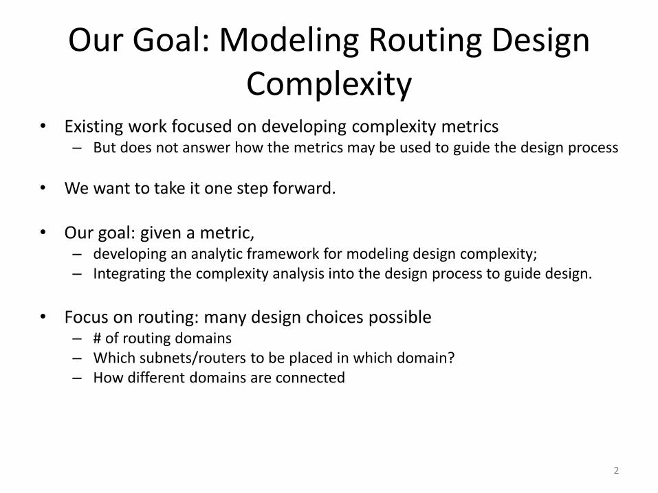
Our Goal: Modeling Routing Design Complexity
• Existing work focused on developing complexity metrics – But does not answer how the metrics may be used to guide the design process
• We want to take it one step forward.
• Our goal: given a metric, – developing an analytic framework for modeling design complexity; – Integrating the complexity analysis into the design process to guide design.
• Focus on routing: many design choices possible
– # of routing domains – Which subnets/routers to be placed in which domain? – How different domains are connected
2
What Do We Mean by “Complexity”?
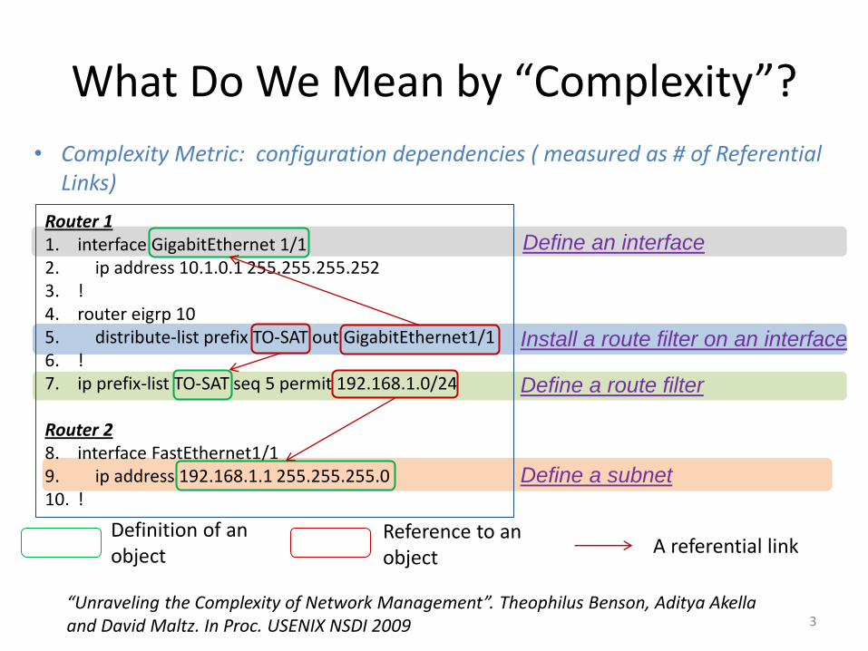
Router 1 1. interface GigabitEthernet 1/1 2. ip address 10.1.0.1 255.255.255.252 3. ! 4. router eigrp 10 5. distribute-list prefix TO-SAT out GigabitEthernet1/1 6. ! 7. ip prefix-list TO-SAT seq 5 permit 192.168.1.0/24 Router 2 8. interface FastEthernet1/1 9. ip address 192.168.1.1 255.255.255.0 10. !
Definition of an object
Reference to an object
A referential link
Install a route filter on an interface
Define a route filter
Define a subnet
Define an interface
3
• Complexity Metric: configuration dependencies ( measured as # of Referential Links)
“Unraveling the Complexity of Network Management”. Theophilus Benson, Aditya Akella and David Maltz. In Proc. USENIX NSDI 2009
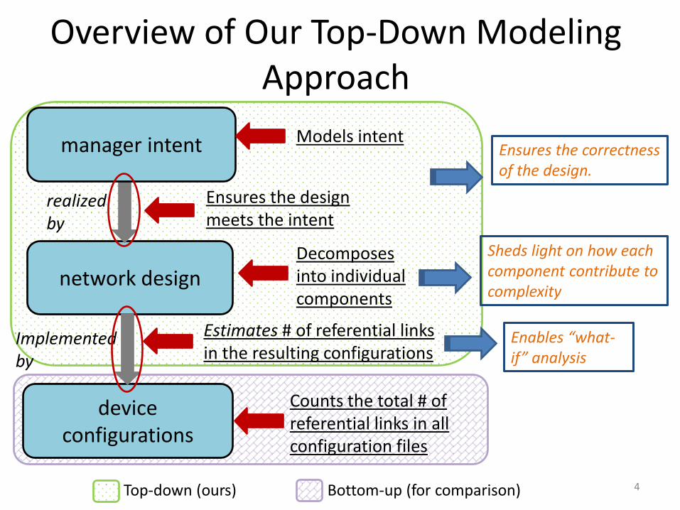
Overview of Our Top-Down Modeling Approach
network design
device configurations
Implemented by
realized by
manager intent
Decomposes into individual components
Ensures the design meets the intent
Sheds light on how each component contribute to complexity
Top-down (ours) Bottom-up (for comparison)
Counts the total # of referential links in all configuration files
Estimates # of referential links in the resulting configurations
Models intent
4
Enables “what-if” analysis
Ensures the correctness of the design.

Agenda
• Overview of our research goal & approach
• Abstractions we leveraged for..
– decomposing routing design
– capturing operators high-level intent
• Modeling details
• An evaluation study using the campus network of a large U.S. university
5
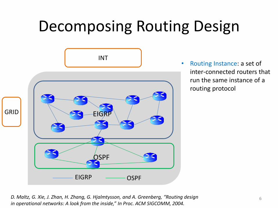
Decomposing Routing Design
EIGRP OSPF
INT
EIGRP
OSPF
GRID
D. Maltz, G. Xie, J. Zhan, H. Zhang, G. Hjalmtysson, and A. Greenberg, “Routing design in operational networks: A look from the inside,” In Proc. ACM SIGCOMM, 2004.
• Routing Instance: a set of inter-connected routers that run the same instance of a routing protocol
6
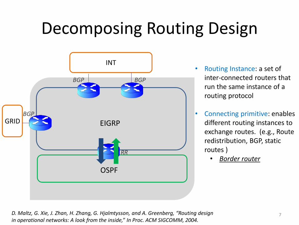
Decomposing Routing Design
INT
EIGRP
OSPF
GRID
D. Maltz, G. Xie, J. Zhan, H. Zhang, G. Hjalmtysson, and A. Greenberg, “Routing design in operational networks: A look from the inside,” In Proc. ACM SIGCOMM, 2004.
BGP BGP
BGP
RR
• Routing Instance: a set of inter-connected routers that run the same instance of a routing protocol
• Connecting primitive: enables different routing instances to exchange routes. (e.g., Route redistribution, BGP, static routes ) • Border router
7
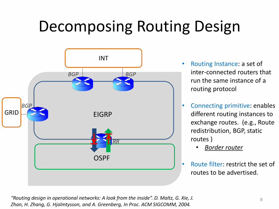
Decomposing Routing Design
INT
EIGRP
OSPF
GRID
• Routing Instance: a set of inter-connected routers that run the same instance of a routing protocol
• Connecting primitive: enables different routing instances to exchange routes. (e.g., Route redistribution, BGP, static routes ) • Border router
• Route filter: restrict the set of
routes to be advertised.
“Routing design in operational networks: A look from the inside”. D. Maltz, G. Xie, J. Zhan, H. Zhang, G. Hjalmtysson, and A. Greenberg, In Proc. ACM SIGCOMM, 2004.
BGP BGP
BGP
RR
8
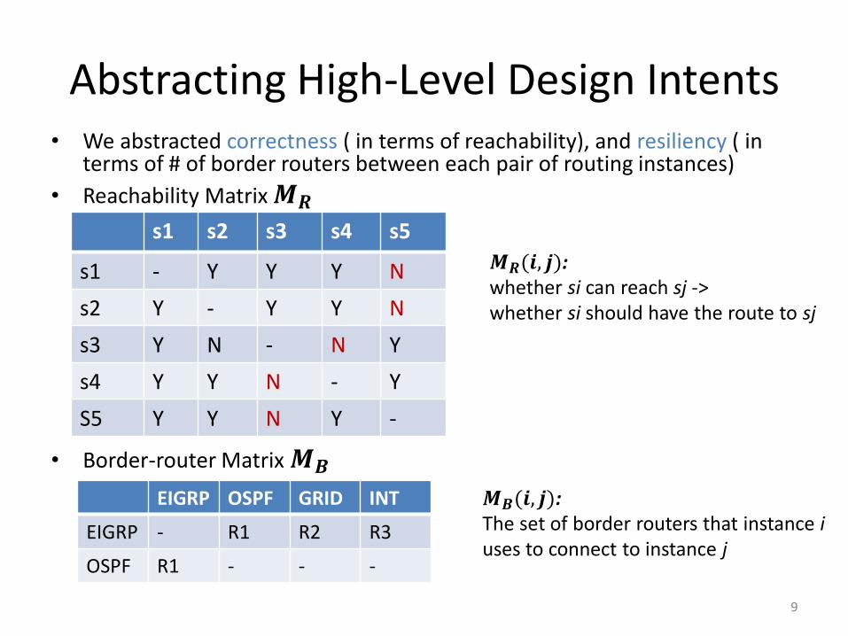
Abstracting High-Level Design Intents • We abstracted correctness ( in terms of reachability), and resiliency ( in
terms of # of border routers between each pair of routing instances)
• Reachability Matrix 𝑴𝑹
• Border-router Matrix 𝑴𝑩
𝑴𝑹(𝒊, 𝒋): whether si can reach sj -> whether si should have the route to sj
EIGRP OSPF GRID INT
EIGRP - R1 R2 R3
OSPF R1 - - -
s1 s2 s3 s4 s5
s1 - Y Y Y N
s2 Y - Y Y N
s3 Y N - N Y
s4 Y Y N - Y
S5 Y Y N Y -
𝑴𝑩(𝒊, 𝒋): The set of border routers that instance i uses to connect to instance j
9
Agenda
• Overview of our research goal & approach
• Abstractions we leveraged for..
– decomposing routing design
– capturing operators high-level intent
• Modeling Details
• An evaluation study using the campus network of a large U.S. university
10
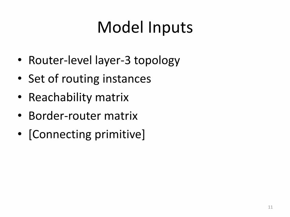
Model Inputs
• Router-level layer-3 topology
• Set of routing instances
• Reachability matrix
• Border-router matrix
• [Connecting primitive]
11
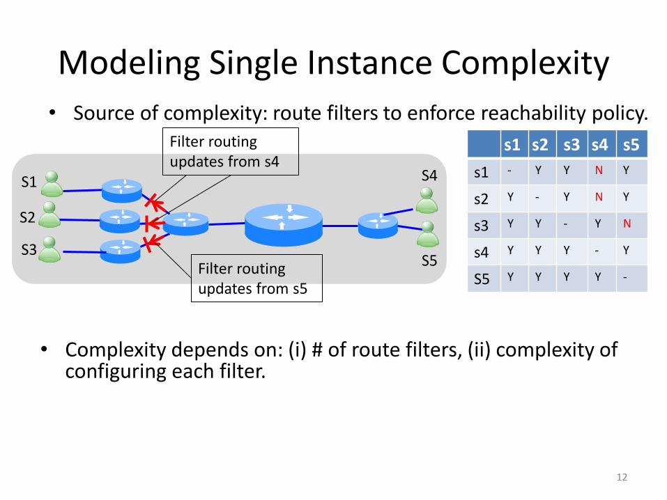
Modeling Single Instance Complexity • Source of complexity: route filters to enforce reachability policy.
S4 S1
S2
S5 S3
s1 s2 s3 s4 s5
s1 - Y Y N Y
s2 Y - Y N Y
s3 Y Y - Y N
s4 Y Y Y - Y
S5 Y Y Y Y -
Filter routing updates from s4
Filter routing updates from s5
• Complexity depends on: (i) # of route filters, (ii) complexity of configuring each filter.
12
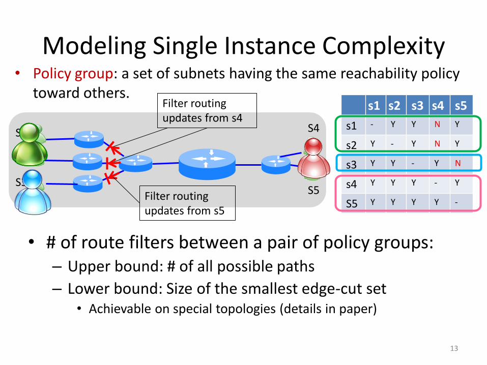
Modeling Single Instance Complexity • Policy group: a set of subnets having the same reachability policy
toward others.
S4 S1
S2
S5 S3
s1 s2 s3 s4 s5
s1 - Y Y N Y
s2 Y - Y N Y
s3 Y Y - Y N
s4 Y Y Y - Y
S5 Y Y Y Y -
Filter routing updates from s4
Filter routing updates from s5
• # of route filters between a pair of policy groups: – Upper bound: # of all possible paths
– Lower bound: Size of the smallest edge-cut set • Achievable on special topologies (details in paper)
13
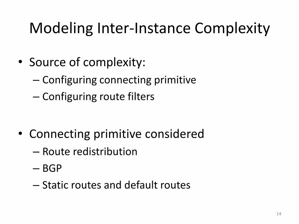
Modeling Inter-Instance Complexity
• Source of complexity:
– Configuring connecting primitive
– Configuring route filters
• Connecting primitive considered
– Route redistribution
– BGP
– Static routes and default routes
14
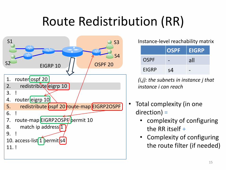
Route Redistribution (RR)
EIGRP 10 OSPF 20
1. router ospf 20 2. redistribute eigrp 10 3. ! 4. router eigrp 10 5. redistribute ospf 20 route-map EIGRP2OSPF 6. ! 7. route-map EIGRP2OSPF permit 10 8. match ip address 1 9. ! 10. access-list 1 permit s4 11. !
• Total complexity (in one direction) = • complexity of configuring
the RR itself + • Complexity of configuring
the route filter (if needed)
15
OSPF EIGRP
OSPF - all
EIGRP s4 -
(i,j): the subnets in instance j that instance i can reach
S3 S1
S2
S4
Instance-level reachability matrix

More Complexity with Multiple Border Routers
• Route feedback could occur – May cause forwarding loop – Determining whether forwarding loop will occur is NP-hard.
[Understanding Route Redistribution, F. Le, G. Xie and H. Zhang, ICNP 2007]
• Solution: using route filters on all the border routers to prevent
feedback.
• We assume that route filters will always be used in this case.
16
EIGRP 10 OSPF 20
S3 S1
S2
S4
R1
R2
Agenda
• Overview of our research goal & approach
• Abstractions we leveraged for..
– decomposing routing design
– capturing operators high-level intent
• Modeling Details
• An evaluation study using the campus network of a large U.S. university
17
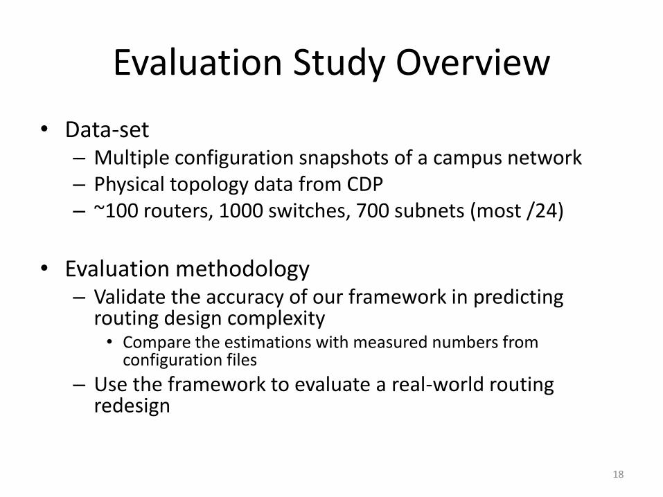
Evaluation Study Overview
• Data-set – Multiple configuration snapshots of a campus network – Physical topology data from CDP – ~100 routers, 1000 switches, 700 subnets (most /24)
• Evaluation methodology
– Validate the accuracy of our framework in predicting routing design complexity • Compare the estimations with measured numbers from
configuration files
– Use the framework to evaluate a real-world routing redesign
18
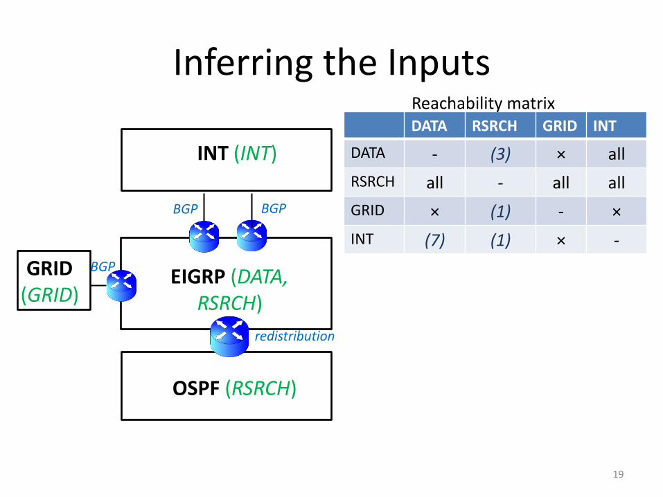
Inferring the Inputs
DATA RSRCH GRID INT
DATA - (3) × all
RSRCH all - all all
GRID × (1) - ×
INT (7) (1) × -
Reachability matrix
19
GRID (GRID)
BGP
BGP
INT (INT)
EIGRP (DATA,
OSPF (RSRCH)
BGP
RSRCH)
redistribution
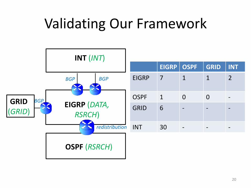
Validating Our Framework
EIGRP OSPF GRID INT
EIGRP 7 1 1
2
OSPF 1 0 0 -
GRID 6
- - -
INT 30 - - -
GRID (GRID)
BGP
BGP
INT (INT)
EIGRP (DATA,
OSPF (RSRCH)
BGP
RSRCH)
redistribution
20
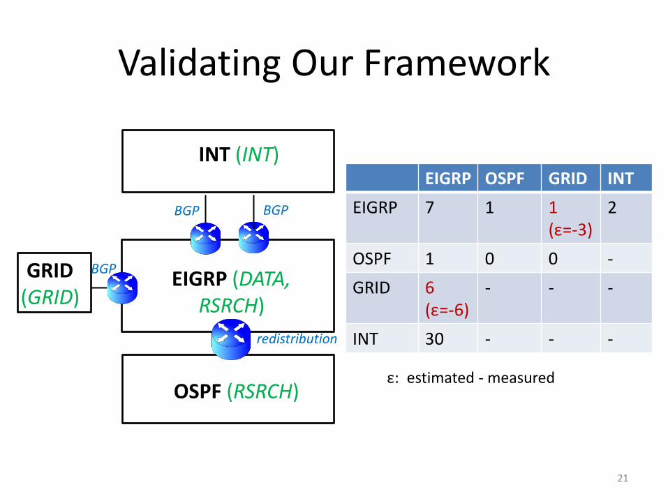
Validating Our Framework
EIGRP OSPF GRID INT
EIGRP 7 1 1 (ε=-3)
2
OSPF 1 0 0 -
GRID 6 (ε=-6)
- - -
INT 30 - - -
ε: estimated - measured
GRID (GRID)
BGP
BGP
INT (INT)
EIGRP (DATA,
OSPF (RSRCH)
BGP
RSRCH)
redistribution
21

Case Study of a Redesign
• Move RSRCH to OSPF
• OSPF now has two border routers
• Uses static routes instead
• Grid now peers with OSPF
BGP
Static routes
GRID (GRID)
BGP
INT (INT)
EIGRP (DATA,
OSPF (RSRCH)
BGP
RSRCH)
redistribution
22
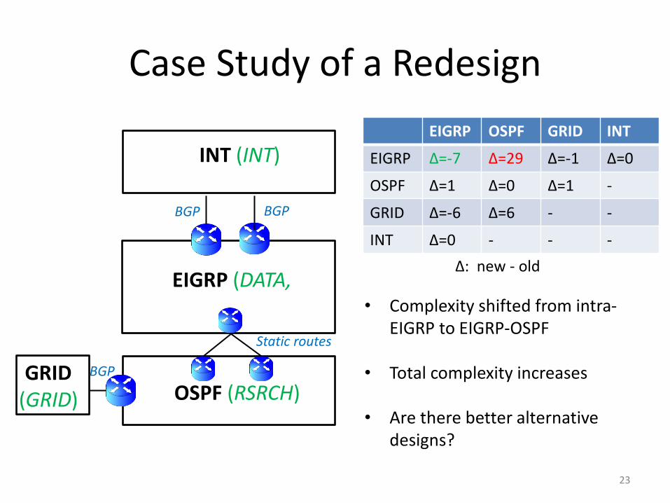
Case Study of a Redesign
BGP
Static routes
GRID (GRID)
BGP
INT (INT)
EIGRP (DATA,
OSPF (RSRCH)
BGP
EIGRP OSPF GRID INT
EIGRP Δ=-7 Δ=29 Δ=-1 Δ=0
OSPF Δ=1 Δ=0 Δ=1 -
GRID Δ=-6 Δ=6 - -
INT Δ=0 - - -
Δ: new - old
• Complexity shifted from intra-EIGRP to EIGRP-OSPF
• Total complexity increases
• Are there better alternative designs?
23
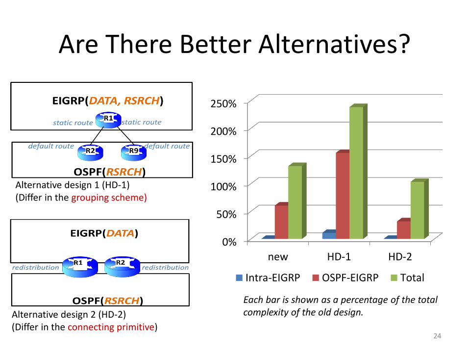
Are There Better Alternatives?
Alternative design 1 (HD-1) (Differ in the grouping scheme)
Alternative design 2 (HD-2) (Differ in the connecting primitive)
0%
50%
100%
150%
200%
250%
new HD-1 HD-2
Intra-EIGRP OSPF-EIGRP Total
24
Each bar is shown as a percentage of the total complexity of the old design.
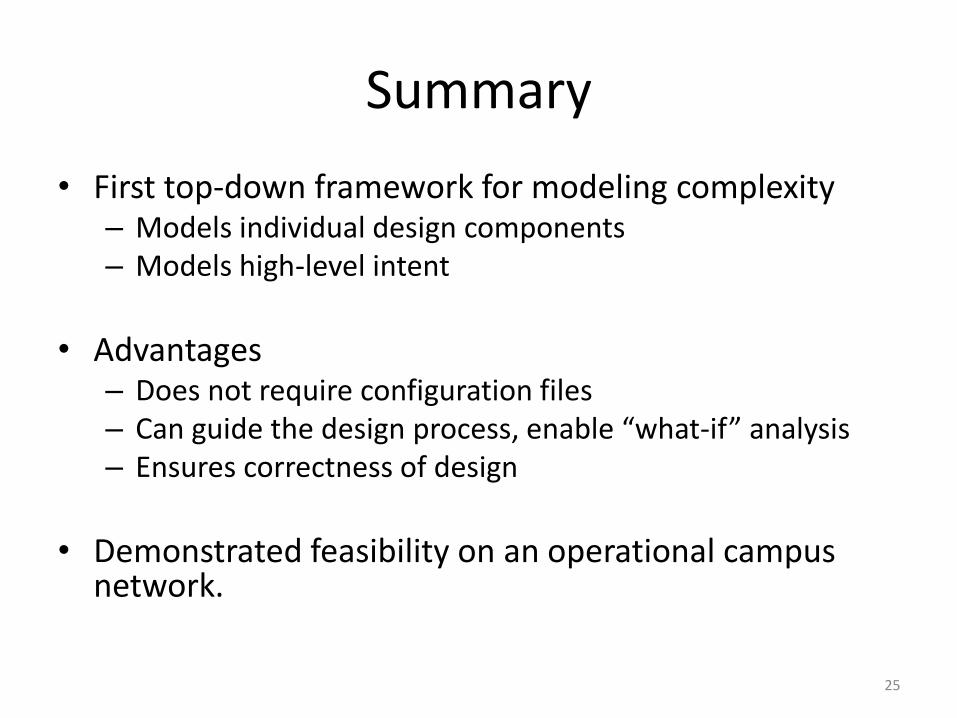
Summary
• First top-down framework for modeling complexity – Models individual design components – Models high-level intent
• Advantages
– Does not require configuration files – Can guide the design process, enable “what-if” analysis – Ensures correctness of design
• Demonstrated feasibility on an operational campus
network.
25
Future Directions
• Complexity-aware top-down routing design – By leveraging the models developed here to guide the search
• Taking into account other design objectives (costs,
performance, etc.) and design constraints (hardware capacity, etc.)
• Jointly optimize across multiple design tasks – VLANs, packet filters, etc.
• Emerging architectures and configuration languages.
26
Thank you!
• Modeling
27
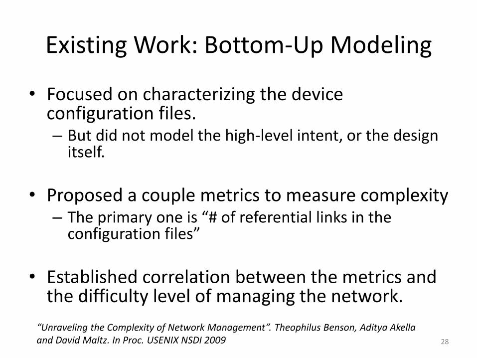
Existing Work: Bottom-Up Modeling
• Focused on characterizing the device configuration files. – But did not model the high-level intent, or the design
itself.
• Proposed a couple metrics to measure complexity – The primary one is “# of referential links in the
configuration files”
• Established correlation between the metrics and the difficulty level of managing the network.
“Unraveling the Complexity of Network Management”. Theophilus Benson, Aditya Akella and David Maltz. In Proc. USENIX NSDI 2009 28
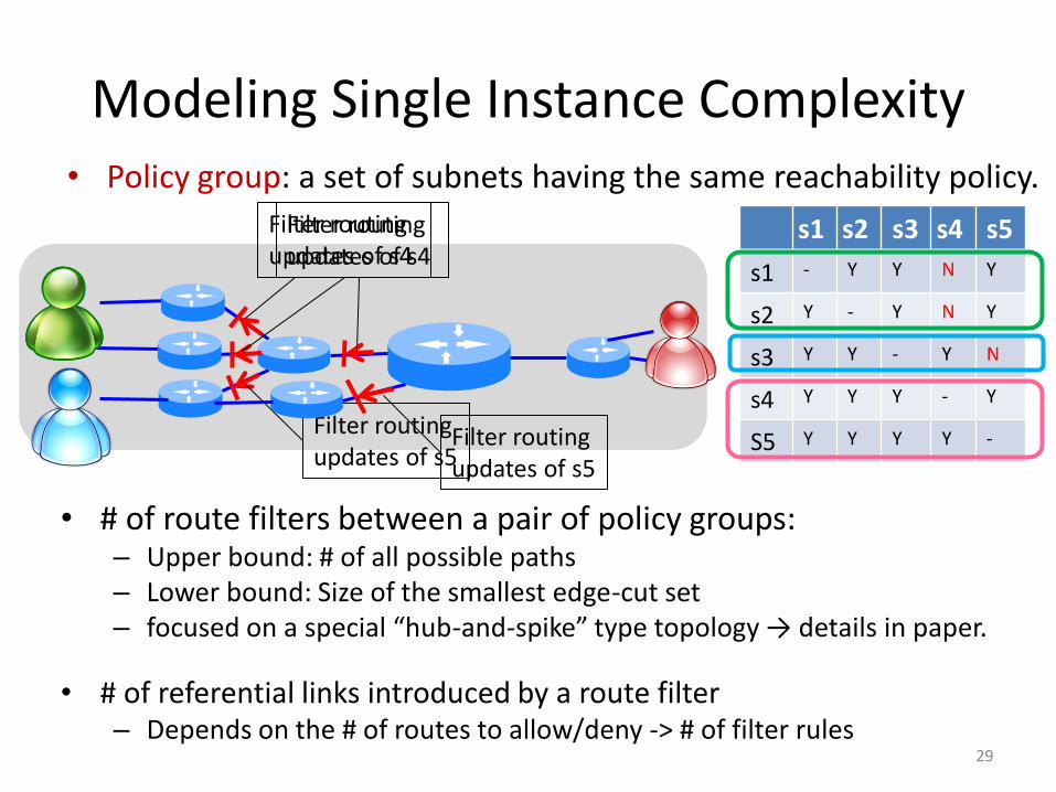
Modeling Single Instance Complexity • Policy group: a set of subnets having the same reachability policy.
s1 s2 s3 s4 s5
s1 - Y Y N Y
s2 Y - Y N Y
s3 Y Y - Y N
s4 Y Y Y - Y
S5 Y Y Y Y -
Filter routing updates of s4
Filter routing updates of s5
• # of route filters between a pair of policy groups: – Upper bound: # of all possible paths – Lower bound: Size of the smallest edge-cut set – focused on a special “hub-and-spike” type topology → details in paper.
• # of referential links introduced by a route filter – Depends on the # of routes to allow/deny -> # of filter rules
29
Filter routing updates of s4
Filter routing updates of s5
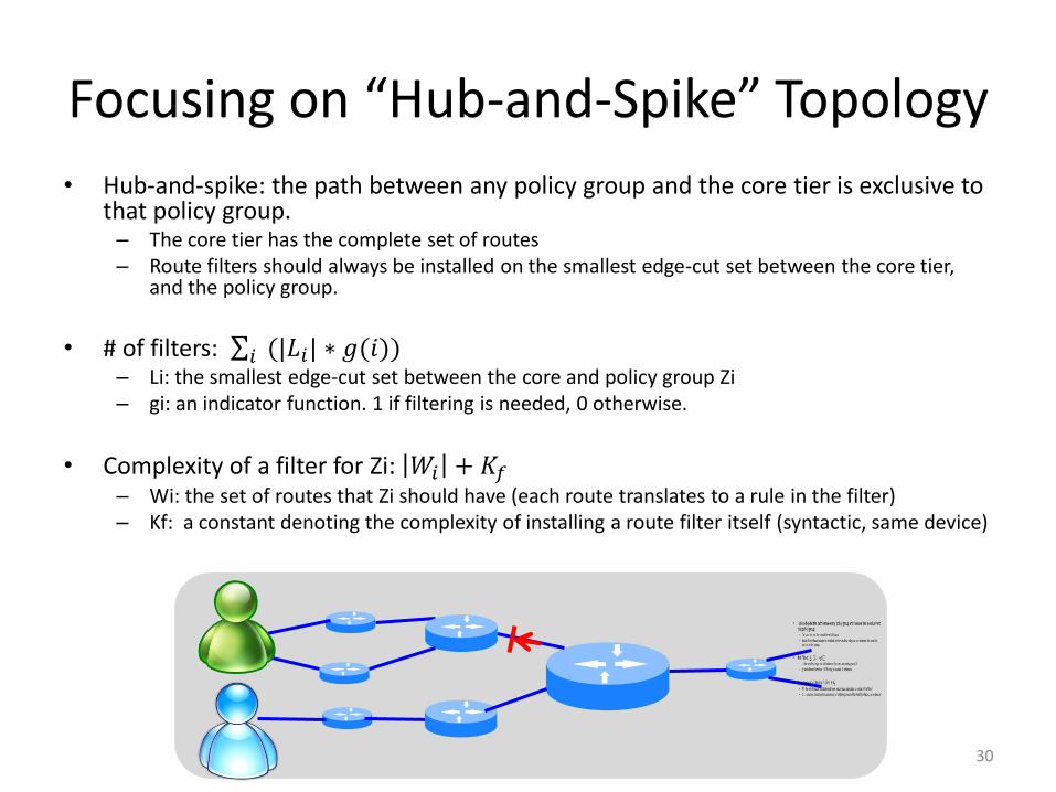
Focusing on “Hub-and-Spike” Topology
• Hub-and-spike: the path between any policy group and the core tier is exclusive to that policy group. – The core tier has the complete set of routes – Route filters should always be installed on the smallest edge-cut set between the core tier,
and the policy group.
• # of filters: (|𝐿𝑖| ∗ 𝑔(𝑖))𝑖
– Li: the smallest edge-cut set between the core and policy group Zi – gi: an indicator function. 1 if filtering is needed, 0 otherwise.
• Complexity of a filter for Zi: 𝑊𝑖 + 𝐾𝑓 – Wi: the set of routes that Zi should have (each route translates to a rule in the filter) – Kf: a constant denoting the complexity of installing a route filter itself (syntactic, same device)
30
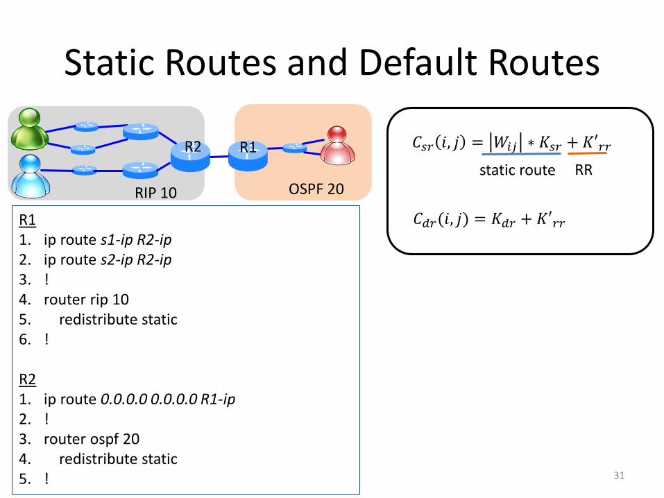
Static Routes and Default Routes
RIP 10 OSPF 20
R1 1. ip route s1-ip R2-ip 2. ip route s2-ip R2-ip 3. ! 4. router rip 10 5. redistribute static 6. ! R2 1. ip route 0.0.0.0 0.0.0.0 R1-ip 2. ! 3. router ospf 20 4. redistribute static 5. !
𝐶𝑠𝑟 𝑖, 𝑗 = 𝑊𝑖𝑗 ∗ 𝐾𝑠𝑟 + 𝐾′𝑟𝑟 R2 R1
static route RR
𝐶𝑑𝑟(𝑖, 𝑗) = 𝐾𝑑𝑟 + 𝐾′𝑟𝑟
31
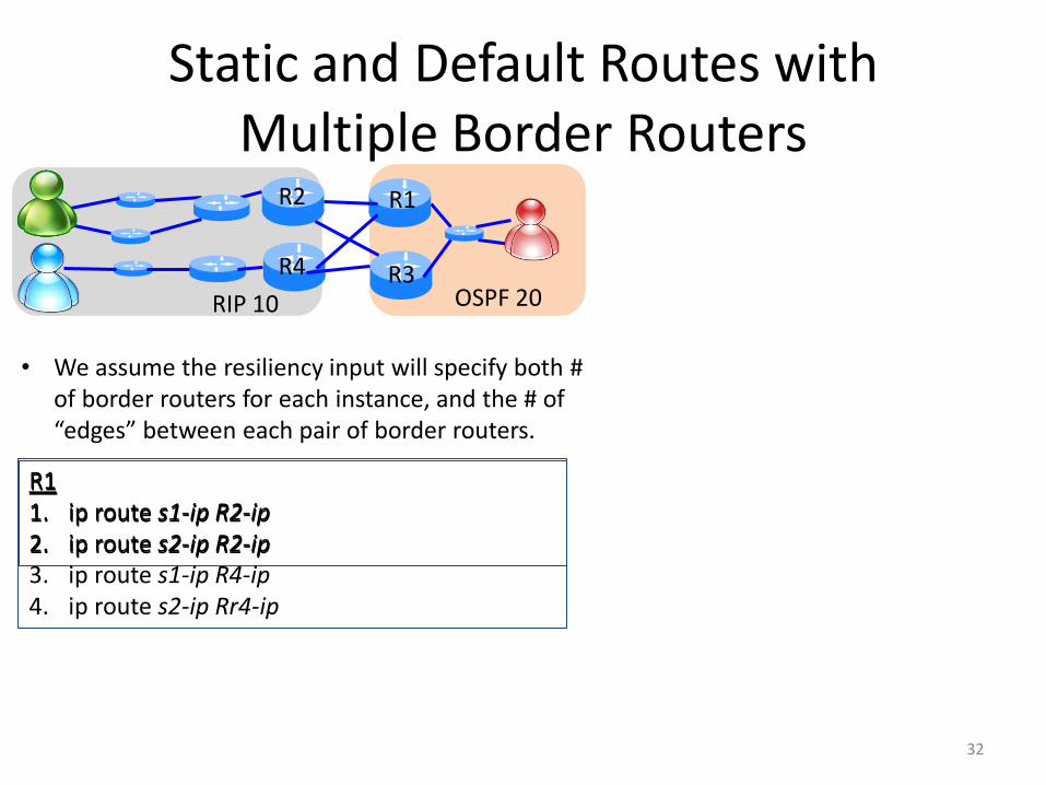
Static and Default Routes with Multiple Border Routers
RIP 10 OSPF 20
R2 R1
R4 R3
• We assume the resiliency input will specify both # of border routers for each instance, and the # of “edges” between each pair of border routers.
R1 1. ip route s1-ip R2-ip 2. ip route s2-ip R2-ip
R1 1. ip route s1-ip R2-ip 2. ip route s2-ip R2-ip 3. ip route s1-ip R4-ip 4. ip route s2-ip Rr4-ip
32
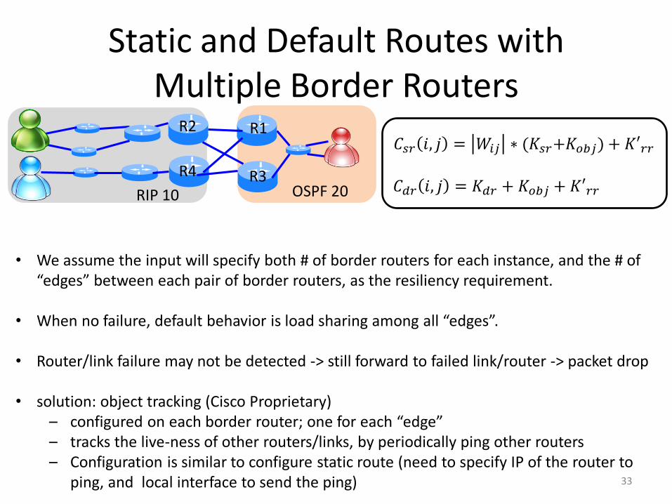
Static and Default Routes with Multiple Border Routers
RIP 10 OSPF 20
R2 R1
R4 R3
• We assume the input will specify both # of border routers for each instance, and the # of “edges” between each pair of border routers, as the resiliency requirement.
• When no failure, default behavior is load sharing among all “edges”.
• Router/link failure may not be detected -> still forward to failed link/router -> packet drop
• solution: object tracking (Cisco Proprietary) – configured on each border router; one for each “edge” – tracks the live-ness of other routers/links, by periodically ping other routers – Configuration is similar to configure static route (need to specify IP of the router to
ping, and local interface to send the ping)
𝐶𝑠𝑟 𝑖, 𝑗 = 𝑊𝑖𝑗 ∗ (𝐾𝑠𝑟+𝐾𝑜𝑏𝑗) + 𝐾′𝑟𝑟
𝐶𝑑𝑟 𝑖, 𝑗 = 𝐾𝑑𝑟 + 𝐾𝑜𝑏𝑗 + 𝐾′𝑟𝑟
33
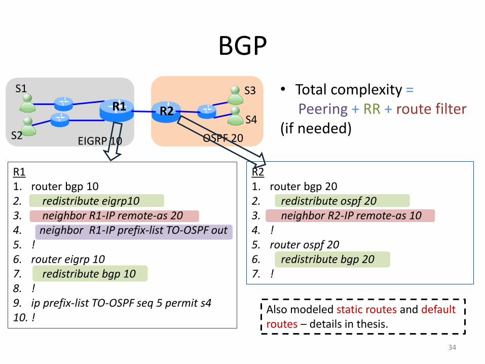
BGP
R1 1. router bgp 10 2. redistribute eigrp10 3. neighbor R1-IP remote-as 20 4. neighbor R1-IP prefix-list TO-OSPF out 5. ! 6. router eigrp 10 7. redistribute bgp 10 8. ! 9. ip prefix-list TO-OSPF seq 5 permit s4 10. !
R2 1. router bgp 20 2. redistribute ospf 20 3. neighbor R2-IP remote-as 10 4. ! 5. router ospf 20 6. redistribute bgp 20 7. !
• Total complexity = Peering + RR + route filter (if needed)
34
EIGRP 10 OSPF 20
S3 S1
S2
S4 R1 R2
Also modeled static routes and default routes – details in thesis.
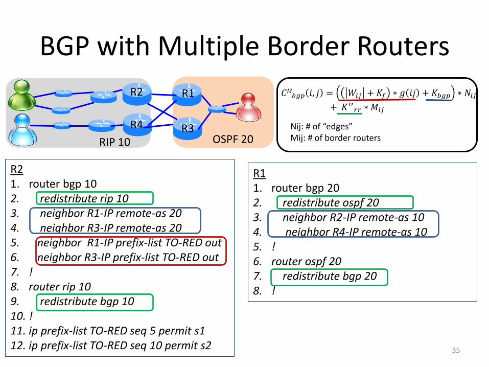
BGP with Multiple Border Routers
R2 1. router bgp 10 2. redistribute rip 10 3. neighbor R1-IP remote-as 20 4. neighbor R3-IP remote-as 20 5. neighbor R1-IP prefix-list TO-RED out 6. neighbor R3-IP prefix-list TO-RED out 7. ! 8. router rip 10 9. redistribute bgp 10 10. ! 11. ip prefix-list TO-RED seq 5 permit s1 12. ip prefix-list TO-RED seq 10 permit s2
R1 1. router bgp 20 2. redistribute ospf 20 3. neighbor R2-IP remote-as 10 4. neighbor R4-IP remote-as 10 5. ! 6. router ospf 20 7. redistribute bgp 20 8. !
𝐶𝑀𝑏𝑔𝑝 𝑖, 𝑗 = 𝑊𝑖𝑗 + 𝐾𝑓 ∗ 𝑔 𝑖𝑗 + 𝐾𝑏𝑔𝑝 ∗ 𝑁𝑖𝑗
+ 𝐾′′𝑟𝑟 ∗ 𝑀𝑖𝑗
RIP 10 OSPF 20
R2 R1
R4 R3 Nij: # of “edges” Mij: # of border routers
35
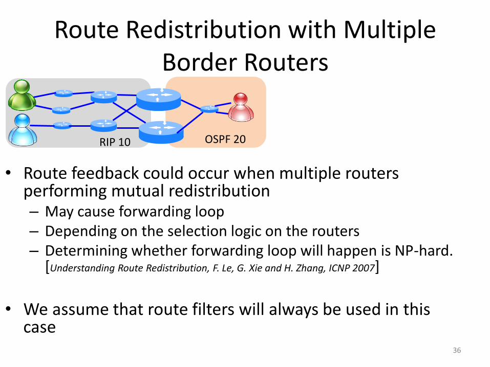
Route Redistribution with Multiple Border Routers
• Route feedback could occur when multiple routers performing mutual redistribution – May cause forwarding loop – Depending on the selection logic on the routers – Determining whether forwarding loop will happen is NP-hard.
[Understanding Route Redistribution, F. Le, G. Xie and H. Zhang, ICNP 2007]
• We assume that route filters will always be used in this
case
RIP 10 OSPF 20
36

Route Redistribution
RIP 10 OSPF 20
1. router rip 10 2. redistribute ospf 20 3. ! 4. router ospf 20 5. redistribute rip 10 route-map RIP2OSPF 6. ! 7. route-map RIP2OSPF permit 10 8. match ip address 1 9. ! 10. access-list 1 permit s1 11. access-list 1 permit s2 12. !
Wij: the set of routes that instance i should advertise to instance j Kf: A constant denoting the complexity of configuring the route filter itself g(ij): An indicator function Krr: A constant denoting the complexity of configuring RR itself.
𝐶𝑟𝑟(𝑖, 𝑗) = ( 𝑊𝑖𝑗 + 𝐾𝑓) ∗ 𝑔 𝑖𝑗 + 𝐾𝑟𝑟
route filter RR
37
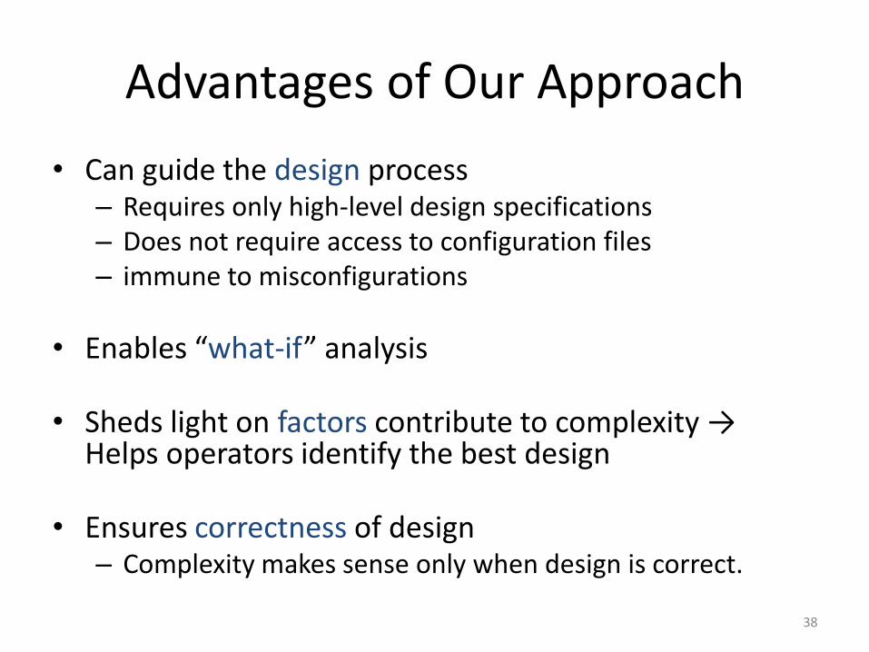
Advantages of Our Approach
• Can guide the design process – Requires only high-level design specifications – Does not require access to configuration files – immune to misconfigurations
• Enables “what-if” analysis
• Sheds light on factors contribute to complexity → Helps operators identify the best design
• Ensures correctness of design – Complexity makes sense only when design is correct.
38