Increasing complexity in hydrologic modeling: an uphill route?
109
Increasing complexity in hydrologic modeling: an uphill route? The influence of complexity on model performance for a physically based, spatially distributed and first order coupled hydrologic model Han Vermue, March 2009
Transcript of Increasing complexity in hydrologic modeling: an uphill route?

Increasing complexity in hydrologic modeling: an uphill route?
The influence of complexity on model performance for a physically based, spatially distributed and first order coupled
hydrologic model
Han Vermue, March 2009


Supervisors Dr.D.C.M. Augustijn Water engineering & management University of Twente Dr. M.J.Booij Water engineering & management University of Twente Ing. J.H.N. Moorman Onderzoek en Monitoring Waterschap Aa en Maas ir.R.G.J Velner Water & Ecologie Royal Haskoning
Increasing complexity in hydrologic modeling: an uphill route?
The influence of complexity on model performance for a physically based, spatially distributed and first order coupled
hydrologic model


Preface I would like to thank the Water Board Aa and Maas and Royal Haskoning in general for giving me the opportunity to do my master thesis and for their support during the process. The possibility to work in both a commercial as governmental environment has given me lots of insight in the differences and similarities between the two institutions. My research would not have been possible without the help of a lot of people. Most notably, my supervisors at the University of Twente, Royal Haskoning and the Water Board Aa and Maas. I would like to thank Martijn, Denie, Roel and Jos for their support and valuable advices during my thesis. Furthermore, I would like to thank Vikesh Bedekar of Hydrogeologic Inc. for giving me valuable and quick responses to the numerous e-mails with the practical issues surrounding MODHMS, Jasper Vrugt for giving me advise and the ability to work with the optimization algorithm SCEM-UA and Jon Mensink for sharing his knowledge about the study area. Last of all I would like to thank my family and friends for their support during my whole study. ‘s-Hertogenbosch, 17 March 2009, Han Vermue

Increasing complexity in hydrologic modelling: An uphill route? - 1 -
Executive summary Climate change and anthropological influences cause changes in hydrological behaviour in several domains of hydrology (groundwater, surface water, unsaturated zone, overland flow). For instance, implemented water retention areas can also have effect on local groundwater levels and damage agricultural interests next to an intended reduction of peak flows. This indicates a demand for insight in the importance of interactions between domains to assess implemented measures. To achieve insight in these processes, hydrological models can be of use. To model these kinds of situations spatially distributed, physically based and preferably first order coupled model concepts are needed. The MODular Hydrologic Modelling System (MODHMS) is such a model concept. The water board Aa en Maas has a desire to obtain more knowledge about their management area. Several model concepts are available in a composed hydrological toolbox (Moorman, 2007) to model the different domains of the management area. At the moment, a model which couples different domains, surface and groundwater for instance, misses in the toolbox. To be able to study the interactions between the domains MODHMS is purchased. By modelling their management area in MODHMS the Water Board wants to achieve more knowledge about their catchment. Physically based, spatially distributed models often are recognized for having great potential in describing hydrological behaviour. The large numbers of parameters do, however, bring up a great challenge. A lot of choices need to be made, from discretization to calculation steps and choice of parameters and processes which will be modelled. Beven (2001) summarises problems associated with spatial distributed modelling. These problems are problems regarding nonlinearity, scale, uncertainty and equifinality. The effect of these problems is that more complex models do not per definition generate better results. Therefore it is interesting if there is a complexity at which model performance is optimal. Several compositions of the study area can be chosen which could perform equally well considering certain objectives. In this research the catchment of the Astense Aa, located in the province of Noord-Brabant in the Netherlands, in the influence area of Water Board Aa and Maas has been modelled in different complexities in MODHMS. The objective in this research was to analyze the influence of adding complexity on model performance and possibly find an optimum complexity considering model performance. The different complexities were analyzed for their influence on model performance, first using a comparison between complexity steps with equal parameter values. This showed the influence of the added complexity as other factors were kept constant. Secondly, calibration parameter values were optimized using an optimization algorithm after which a validation run was done on which model performance was based. This result was used as best possible simulation with the given complexity. Model performance was based on the capability of the model to reproduce measured discharges and spatially distributed phreatic groundwater heads. The different complexity steps are composed of a very simple lumped model consisting of 1 reservoir to a, as most complex step, spatially distributed model composed of a geological fault, 2 aquifers and detailed description of the surface water system with first-order coupling to the groundwater domain. Due to time restrictions it was not possible to test more complex models including unsaturated zone, van Genuchten, equations and an overland flow domain. The results were characterized by a lack of evapotranspiration resulting in a water balance error causing groundwater levels and discharges to be significantly overestimated. The researched complexities lacked a thorough description of the evapotranspiration process. Furthermore, the results were influenced by the very simple composition of the models considering discretization. Added complexity caused unexpected changes in hydrological behaviour. This was caused due to the combined effect of the complexity and the chosen discretization and settings. The water balance error has large influences on the results from the optimization algorithm. The parameter values are optimized in such a way that the distribution of the excess of water is least harmful to the model performance. The optimization results do not give information if the introduced complexity is an improvement of the description of the study area, due to the influence of the water balance error and the discretization issue. These problems together with the small amount of tested complexities made it impossible to find a reliable optimum of model complexity regarding model performance. The optimization also showed that the chosen mathematical description of the model performance combined with the characteristics of the groundwater and surface water caused a bias towards optimizing the groundwater levels.

Increasing complexity in hydrologic modelling: An uphill route? - 2 -
The models are not properly composed or not complex enough to describe the water balance terms and therefore overall hydrological behaviour is not simulated well. During optimization there is no calibration parameter which can directly influence the water balance without changing other hydrological behaviour. Thus during the optimization, calibration parameters are chosen in such a way that they compensate for the water balance error which results in a large overestimation of, especially, the discharge (due to the bias towards the groundwater levels). The findings in this research make it clear that when modelling with a physically based, spatially distributed model a certain amount or composition of complexity is required as starting point. This is necessary to be able to compare the different complexities on model performance without having to deal with water balance errors or discretization issues. The influence of added complexity can be researched with the current method only the starting models should be adjusted. Furthermore, the mathematical definition of the model performance needs to be changed to equally weigh the discharge and groundwater levels in the optimization. However, it is not possible to make a statement about if the new complexity is an improvement of the description of the study area due to the problems with the water balance error. The optimization should include a calibration parameter to have a degree of freedom to correct for water balance errors, possibly the evapotranspiration process should be described in a more complex way. Furthermore, to avoid problems with discretization a certain amount of layers in the subsurface should be implemented at the beginning.
Increasing complexity in hydrologic modelling: An uphill route? - 3 -
Table of contents
1 INTRODUCTION - 5 - 1.1 Background and framework - 5 -
1.2 Problem analysis - 5 -
1.3 Objective and research questions - 6 -
1.4 Research method - 8 -
1.5 Outline of this report - 9 -
2 CATCHMENT OF THE ASTENSE AA - 10 - 2.1 Overview and surface water network - 10 -
2.2 Water balance - 13 -
2.3 Meteorology - 14 -
2.4 Hydrology - 14 -
2.5 Hydrogeology - 17 -
3 METHODOLOGY FOR DETERMINING INFLUENCE OF COMPLEXITY - 20 - 3.1 MODHMS - 20 -
3.2 Selection calibration and validation period - 26 -
3.3 Selection of observation points - 27 -
3.4 Mathematical description of model performance - 28 -
3.5 Spatial and temporal discretization - 29 -
3.6 Parameterization - 30 -
3.7 Stepwise implementation of complexity - 33 -
3.8 Analyzing influence complexity - 39 -
4 RESULTS - 41 - 4.1 Comparison using equal parameter values - 41 -
4.2 Determining the best model performance per step - 47 -
4.3 Comparison with the WAGENINGEN model - 53 -
5 DISCUSSION - 55 - 5.1 Is MODHMS an appropriate tool to obtain more water system knowledge? - 55 -
5.2 Using groundwater recharge instead of precipitation on step 1 - 56 -
5.3 Optimization algorithm and objective functions - 57 -
5.4 Lack of variation in discharge results - 58 -
5.5 Methodology and influence of further steps - 60 -
6 CONCLUSIONS AND RECOMMENDATIONS - 61 - 6.1 Conclusion - 61 -
6.2 Recommendations - 62 -
BIBLIOGRAPHY - 63 -

Increasing complexity in hydrologic modelling: An uphill route? - 4 -
APPENDICES - 67 -
1 GROUNDWATER EXTRACTION - 68 -
2 EVAPOTRANSPIRATION - 69 -
3 SENSITIVITY ANALYSIS - 72 -
4 OPTIMIZATION ALGORITHM - 74 -
5 STEPWISE IMPLEMENTATION OF COMPLEXITY - 78 -
6 RESULT CALIBRATION AFTER OPTIMIZATION PARAMETER VALUES - 96 -
7 RESULTS STEP 1 TO 2 EXCHANGE - 98 -
8 RESULTS 2 TO 3 SEPARATED - 99 -
9 RESULTS STEP 2 TO 3 WITH EXTRA LAYER - 101 -
10 DISCUSSION USING GROUNDWATER RECHARGE INSTEAD OF PRECIPITATION - CALIBRATION RESULTS - 102 -
11 DISCUSSION CHANNEL FLOW MODULE - 104 -

Increasing complexity in hydrologic modelling: An uphill route? - 5 -
1 Introduction The problem analysis and the motive for this research are explained in this chapter. Furthermore, the problem analysis is converted into an objective and research question. In 1.4 a brief introduction into the main aspects of the research method is shown. In 1.5 the structure of the report is described.
1.1 Background and framework Climate change and anthropological influences can influence several aspects of the hydrological processes. This causes a demand for better understanding of the relation between these hydrological processes. The conflicting interests about in what way water management needs to be applied indicates the need for more knowledge about how scenarios, measures and management affect the hydrology. For instance, restoring the original path of a creek might influence groundwater levels at a nearby located farm, which might threat productivity. Therefore, more insight in the relations between different domains in hydrology is desired, to be able to better approximate the effects of (climate) scenarios and measures. Hydrological modelling concepts can help in understanding hydrological processes. Several hydrological models are available which can be classified in different classes. Models can be classified conceptual or physically based depending on their theoretical support. Furthermore, models can be classified lumped (if all parameters are spatially averaged over the catchment) or spatially distributed (using e.g. a grid). The class of the model partially determines the application of the model. The situation defined in the first paragraph indicates that a spatially distributed model should be used. The Water Board Aa en Maas, which supervises the hydrological related processes in the south east part of the province Noord-Brabant, is experiencing problems like stated in the first paragraph. The current description and modelling of a catchment of the Water Board comprises several different models. For instance, for generating discharges from small parts of the catchment the lumped, conceptual WAGENINGEN model is used (Velner et al.(2008a); Velner et al. (2008b)). For a description of the WAGENINGEN model is referred to Warmerdam et al. (1996). For routing high water flows through the larger rivers in the catchment, a Sobek1D2D (Deltares, 2009) model is used. Furthermore, Modflow (McDonald & Harbaugh, 1988) models are used to model groundwater heads and flow. The Water Board Aa en Maas has compiled a hydrological toolbox in which data and models are centred in one place (Moorman, 2007). The Water Board Aa en Maas wants to improve their knowledge of their management area to be able to anticipate on future challenges. One aspect of this is the importance of the interaction between domains. The current set of models primarily describes one domain of the hydrological process. Practical and theoretical issues make it hard to couple the current set of models. Therefore, it is hard to get insight in the interactions between groundwater, unsaturated zone, overland flow and surface water. The Water Board therefore has acquired a new model concept, the MODular Hydrologic Modeling System (MODHMS). By generating models in this concept insight in these processes and their importance can be obtained as it is a physically based, spatially distributed and first order coupled model containing all relevant domains. MODHMS can therefore be an asset and addition to the current selection of models available to the Water Board Aa en Maas. The model can fulfil a function in the objective of the Water Board Aa en Maas to gain more knowledge about their catchment area by simulating the interactions between domains in the catchment. Spatially distributed modelling inherently introduces a lot of parameters. When different domains are used the amount of parameters expands even further. Beven (2001) summarizes the general problems which occur when using spatially distributed models. Problems with uncertainty, nonlinearity, scale and equifinality cause that more complex models do not per definition generate better results. The numerous degrees of freedom available in spatially distributed modelling causes that there are a lot of available configurations possible to model the study area. This brings up the question if there is some sort of optimum configuration or complexity at which the model gives the best results.
1.2 Problem analysis The model concept of MODHMS can be a useful addition to the current selection of models provided that it gives good and reliable outcomes when compared to measurement data and other model

Increasing complexity in hydrologic modelling: An uphill route? - 6 -
outcomes. As its application is primarily found in problems where interactions are assumed to be essential, quite a number of parameters are needed to model the catchment area. This brings up the question what kind of detail should be used to get good results. Which processes and parameters are important to model and when is adding more parameters and processes no longer needed? The increasing complexity might even diminish the performance of the model. Some general problems with distributed hydrological modelling are summarized by Beven (2001). These are the problems of nonlinearity, scale, equifinality and uncertainty. The problem of nonlinearity can be described as the mismatch between the used equation and the used parameter value. The averaged parameter value, for that grid cell, will not describe the variation within the grid cell and therefore might not capture the dominant value. The equation on the other hand is not appropriate to deal with this local variation and is thus not appropriate. The problem of scale is related to the problem of nonlinearity. The different scales of the process, measurement and model present difficulties in how to aggregate these into one value. The problem of equifinality is the problem of several optimal solutions which can arise from a calibration process. Several parameter sets might produce equally satisfying results considering the objective function. The problem of uniqueness/uncertainty is how the outcomes of a modelling exercise should be interpreted. Adding data and processes, which can be interpreted as adding complexity to the model, might not improve its performance because of the problems stated above. This leads to the question at which point the model performs best. Thus, when does adding complexity no longer improves the model performance as a result of problems as uncertainty, equifinality, scale and nonlinearity? Rientjes and Zaadnoordijk (2000) also describe the problems stated above and state that there is an over parameterisation of models, or in other words that these models are too complex. The problem definition for this research is: Does adding complexity to a spatially distributed model improve the description of the catchment area (in this case the Astense Aa), and thus provide more insight? In this problem definition it is primarily of importance to define what complexity is and what more insight is. This is described in 1.3. Multiple studies have been performed to find an indication of the optimum of complexity of models. Vreugdenhil (2006) investigated the development of uncertainty when adding complexity to a model. The starting point was a very simple model. By identifying the uncertain parts of the model, like data and model structure, the model or input data was modified and the model outcome was monitored to judge whether the model performance has improved or not. The catchment area used in this research is the catchment of the Astense Aa. The reason for choosing this catchment is that it is a small catchment, making it easier to comprehend and it is an upstream catchment which limits the influence of other catchments. Several natural areas are present in the catchment. The water management for these areas can potentially conflict with agricultural interests surrounding these natural areas. Interaction between domains is thus of importance in this catchment. Furthermore, this catchment has been studied and modelled in another model, the conceptual WAGENINGEN model (Warmerdam et al., 1996; Velner, 2008a).
1.3 Objective and research questions The objective for this study is: To quantify and analyze the effect of adding complexity to a model of the catchment of the Astense Aa in MODHMS on the model performance, where, within the defined complexities, the goal is to find the highest model performance. The model performance is an indicator of how well the hydrological behaviour of the catchment area is described. The differences in model performances of the complexities provide more insight in the importance of the parameter and process. This will increase the knowledge of the hydrologic behaviour of the catchment area.

Increasing complexity in hydrologic modelling: An uphill route? - 7 -
The central research question is: Does adding complexity in the model of the Astense Aa lead to a better model performance and is it possible to find an optimum in the model performance, and how does the model perform in comparison to the WAGENINGEN model? The definition of the terms complexity and model performance are very important in this study. These terms will be further described in the next sections.
1.3.1 Complexity The definition of complexity in this study is as follows: ‘Complexity is the number and scale of the parameters and processes used in the model.’ In this definition the scale means the amount of detail of a parameter or process in the model. If a parameter is spatially variable instead of uniform, this is a more detailed and, in this definition, complex model. For instance, the groundwater domain can be modelled as one reservoir, which has the same characteristics everywhere. It can also be modelled as several aquifers and aquitards, each having different hydraulic conductivities and resistances. The last situation is a more complex model. The difference in complexity between models is not easily quantifiable (if possible at all). It is possible to state which model is more complex of the two. In this study, the objective is not to quantify the complexity, but to study the influence of complexity on model performance. The definition of complexity explains already how complexity should be added to a model. Either adding a process to a model or scaling down a parameter, making it spatially variable for instance, will add complexity.
1.3.2 Model performance Model performance can be defined in different ways. Vreugdenhil (2006) uses uncertainty as indicator for model performance. Rientjes et al. (1999) uses the outcome of objective functions as indicator. The definition of model performance in this study is: ‘The model performance is the capability of the model to reproduce measured hydrological behaviour of the catchment which is quantified using the Nash-Sutcliffe coefficient of model efficiency.’ The problem analysis states that a better description and more insight of the catchment area are desired. The model performance should therefore indicate how well the hydrological behaviour of the catchment area is described. The hydrological behaviour is, in this study, defined as the development of water levels and discharges both in space and time. The model outcome is tested against measured data of the hydrological behaviour of the catchment to evaluate if the model describes the hydrological behaviour well. The model performance quantifies how well the hydrological behaviour of the catchment area is described and is used to compare complexities. As well as a quantification using objective functions, visual inspection of the development of groundwater levels and discharges compared to measured data is done to research the influence of the complexity. The visual inspection will reveal the specific influence of the complexity, while the quantification gives a more objective statement about the influence of complexity on model performance. Several observation points are defined for groundwater heads and discharge. At these locations Nash-Sutcliffe (NS) coefficients of model efficiency (Nash & Sutcliffe, 1970) are calculated. The NS coefficients are compiled into one indicator of model performance using a certain weighting procedure. The model performance is based on validation results to avoid the effect of the increasing amount of calibration parameters. As more complexity is introduced, more calibration parameters are used. This will cause more degrees of freedom for the calibration to fit the model to the objective functions. Interviews with Water Board Aa en Maas indicated that no special attention needs to be paid to a certain process. The general behaviour is of importance. The NS coefficient does not emphasize certain characteristics of the hydrological process, like high or low flows, and is therefore suitable as indicator of model performance. Furthermore, it is easily interpretable. The mathematical definition of the model performance and NS coefficient can be found in 3.4. The differences in model performance between complexities will increase the knowledge about the catchment, as an indication which processes are important and which are less important.

Increasing complexity in hydrologic modelling: An uphill route? - 8 -
1.4 Research method In Figure 1 an overview is given of the research method that is used in this research. This scheme gives an overview how the influence of complexity on model performance is analyzed and which steps are needed.
Figure 1 Research method (thick line represents the process which is repeated for every complexity step)
From the objective, the terms model performance and complexity are defined, which are already described in 1.3.1 & 1.3.2. Furthermore, a survey and selection of data is done through studying existing reports, interviews and a visit to the catchment area. Using the definitions of complexity and model performance and the selected data, a plan for stepwise implementation of complexity is constructed. Several increasing complexities are modelled to research what the effects are of different model complexities on model performance, and possibly find an optimum. The different complexities will be run with equal parameter values to be able to distinguish the differences in outcomes solely due to the complexity. Furthermore, an optimization algorithm will be run which optimizes the model parameters for the specific complexity step during calibration. These outcomes then will be used to do the validation and give the outcome for the model performance for the specific complexity step. These results are assumed to give the best outcome for the given complexity step. To put the model performance of the MODHMS model in perspective, it is compared to the performance of the WAGENINGEN model. This shows the relative value of the outcomes of MODHMS. Considering the lumped and conceptual nature of the WAGENINGEN model it is by definition impossible to compare spatially variable groundwater heads. Therefore, only discharge out of the area is compared. Together these findings will be used to determine the influence of complexity on the model performance. Model calibration will be performed using an optimization algorithm. The model calibration will fit the model to measurements, but it is very well possible that more parameter sets describe the calibration data equally well within a certain range. The best result, and its parameter set, is then selected and used for validation. The validation result gives more information about the description of the catchment area as the model is not fitted to this data and the result on the objective function is more reliable. The basic model in the stepwise complexity plan uses catchment averaged parameters, just like the WAGENINGEN model. The following step is to make the model spatially distributed, a grid is constructed and elevations are added for every cell. The other parameters are uniform over the catchment area. Furthermore, a very simple representation of the rivers inside the catchment is modelled. After this step, more complexity is added to the spatially distributed model which is described in 3.7. The choice for this sequence of adding complexity is mainly based on assumed importance of parameters and processes.

Increasing complexity in hydrologic modelling: An uphill route? - 9 -
1.5 Outline of this report Chapter two describes the catchment of the Astense Aa. Both hydraulic, hydrologic and geohydrologic aspects are described. Furthermore, the history and relevant infrastructure is mentioned. Chapter 3 focuses on the methodology to analyze the influence of complexity on model performance. This includes the theoretical background of MODHMS. The model setup and other decisions necessary to setup the model are explained in this chapter. Furthermore, the stepwise implementation of the complexity is explained and how the outcomes are analyzed. Chapter 4 contains the results of the research. First, the results when using equal parameter values are presented. Secondly, the results when using the optimization algorithm for every step are shown. The last section of this chapter contains the comparison to the Wageningen model. Chapter 5 contains the discussion about the results and some further investigation on surprising outcomes of the research. In chapter 6 the conclusion and recommendations are presented.

Increasing complexity in hydrologic modelling: An uphill route? - 10 -
2 Catchment of the Astense Aa The catchment of the Astense Aa is described using the several aspects which are important to the hydrological behaviour of the catchment. First an overview of the catchment and the surface water network is given in 2.1. In 2.2, a water balance of the catchment is shown after which the separate factors are analyzed in the next sections. Most of the data in this chapter is extracted from the hydrological database and toolbox of the Water Board Aa en Maas, which is described by Moorman (2007).
2.1 Overview and surface water network The Astense Aa is a creek in the east of the Province of Noord-Brabant in the Netherlands. The Astense Aa is a tributary of the Aa, which in turn belongs to the drainage system of the Meuse (‘Maas’ in Figure 2). The Aa flows to ‘s-Hertogenbosch where it confluences with the Dommel to form the Dieze, which in turn flows into the Meuse just downstream, northwest, of ‘s-Hertogenbosch.
Figure 2 Catchment Aa including the catchment of the Astense Aa (Velner et al., 2008a)
The catchment of the Astense Aa is shown in Figure 3. The catchment area is 56 km2 and has an elevation difference of about 15 meters, ranging from approx. 18 m+ NAP downstream to 33 m+ NAP upstream. The length of the Astense Aa itself is about 17 kilometres. The Astense Aa is named after the city of Asten which lies nearby, but does not belong to the catchment area. A digital elevation map of the catchment is shown in Figure 41; the data for this map was extracted from the AHN, actueel hoogtebestand Nederland (Rijkswaterstaat, 2007).

Increasing complexity in hydrologic modelling: An uphill route? - 11 -
Figure 3 Catchment Astense Aa

Increasing complexity in hydrologic modelling: An uphill route? - 12 -
The most upstream part of the Astense Aa is connected to a channel, kanaal van Deurne. The kanaal van Deurne is connected to the Meuse. During summer months water can be let in to supply water for agricultural needs. The Astense Aa flows past the villages of Neerkant and Liessel and in between Asten and Deurne to the outlet where it flows into the Aa. The Astense Aa is fed by a tributary, the Soeloop, which drains the Deurnese Peel. Both the Astense Aa and Soeloop are about two to three meters wide. The kanaal van Deurne crosses the catchment but is not part of the catchment, although seepage from the channel might influence the water budget and thus the hydrological processes. The amount of seepage is quite uncertain and not known. Land uses in the catchment are mainly agricultural farm and grass-lands. Furthermore, moors are concentrated in the upstream part of the catchment area. These are part of the natural reserve Deurnese Peel. Surrounding these moors are quite large areas of forest. In the upstream areas around the moors, the forest is mainly deciduous. In the downstream part of the catchment, pine forest and mixed forest are more abundant. The Deurnese Peel is part of the program Natura 2000 and is a ‘natte natuurparel’ (wet pearl), which implies certain objectives and restrictions considering the management of these areas, for instance regarding extraction and drainage of water. Another special natural area is de Berken where the Astense Aa meanders freely without restriction (within certain limits). This area is also a wet pearl. In the catchment area of the Astense Aa several projects with nature objectives are executed. In Figure 4, a map of the land uses in the area is shown.
Figure 4 Land uses in catchment Astense Aa
The Deurnese Peel is located in the North East part of the catchment. Just south of Liessel, where the Soeloop confluences with the Astense Aa. The Deurnese Peel lies between the kanaal van Deurne and the Helenavaart. The Helenavaart forms roughly the north-eastern boundary of the catchment. The kanaal van Deurne crosses the catchment, but is not a part of the catchment. During the summer season water is let in at several places in the catchment. The amounts of water are highly uncertain though. Estimates are in the order of 10-2-10-1
m3/s during this season. The amount of water supplied to the system by pumping station ‘t Zinkse was for 2007, 341.000 m3. Sometimes water from the Astense Aa is used to supply the system of the Voordeldonksche Broekloop. This system lies southwest of the catchment of the Astense Aa. The amounts of water supplied to this system are not known precisely, but are according to experts not very large.

Increasing complexity in hydrologic modelling: An uphill route? - 13 -
The villages of Neerkant, Liessel and a small part of Vlierden are inside the catchment area. In 1995/96, a program was undertaken to create better conditions for natural development in the Deurnese Peel. Measures were taken to increase the water levels. Therefore the draining influence of the Soeloop was reduced. Another objective was to make water supply to the agricultural areas possible. In 2.4.3 these measures are more extensively described.
2.2 Water balance In Table 1 a water balance for several years is shown. The surplus is calculated with the following equation:
QET-P Surplus p −= In which: P = precipitation in mm per year ETp = potential evapotranspiration in mm per year Q = discharge in mm per m2 per year Table 1 Water balance
Year Precipitation [mm] Potential evapotranspiration [mm] Discharge [mm] Surplus [mm] 1996 686 548 163 -25 1997 694 594 132 -32 1998 1094 522 440 133 1999 741 602 102* -17
2000 855 552 181 122 Average 814 563 204** 36 *3 months of data missing, if interpolated with average discharge this would be 156 mm
** This equals 0,36 m3/s The time series of these processes is shown in Figure 5.
Figure 5 Time series for several processes
In Figure 5 the meteorological forcing terms, together with the specific discharge out of the system can be seen. All the terms are in mm/day, it becomes apparent that the discharges in 1998 were very high compared to the other years.
Time series
0,00
2,00
4,00
6,00
8,00
10,00
12,00
14,00
16,00
18,00
20,00
apr-
96
okt-9
6
apr-
97
okt-9
7
apr-
98
okt-9
8
apr-
99
okt-9
9
apr-
00
okt-0
0
Date [month-year]
Q, E
Tp [m
m/d
ay]
0,00
20,00
40,00
60,00
80,00
100,00
120,00
140,00
P [m
m/d
ay]
Potential evapotranspirationSpecific discharge outletPrecipitation

Increasing complexity in hydrologic modelling: An uphill route? - 14 -
The specific discharge is calculated by dividing the discharge with the catchment area. This makes it possible to compare discharge to precipitation and evapotranspiration. Since the catchment area has gone through some changes over the years, due to implementation of measures, the discharge time series before 1996 is not representative for the current situation of the catchment. In reality, the actual evapotranspiration, Eact, will not be equal to the potential evapotranspiration. According to literature (Vereniging voor landinrichting, 2000) ETact is around 350 mm for the Netherlands. The presence of forests and moors might influence this as ETact will be higher due to these land uses. The groundwater levels are fairly high which could hint at higher ETact values than the average for the Netherlands. Probably though the water balance will not close and other factors influence the hydrological behaviour in the catchment. Groundwater storage over this period and outflow over the boundaries might cause this (Figure 7 and Figure 8).
2.3 Meteorology In this section, the meteorological forcing terms, precipitation and evapotranspiration, are described. In Figure 42 the precipitation stations together with the chosen evapotranspiration recording stations are shown.
2.3.1 Precipitation Precipitation data are available from two KNMI (Royal Dutch Meteorological Institute) recording stations. The two stations are Deurne and Someren. The stations are spatially the closest to the catchment area. The two stations are located just north and south of the catchment area. The data contains daily values and is shown in Figure 5. The maximum difference for the measured yearly amount of precipitation between the two stations was 25 mm for the period shown in Figure 5.
2.3.2 Evapotranspiration Potential evapotranspiration data are available for two KNMI recording stations, Volkel and Eindhoven. The reference crop evapotranspiration is calculated using the Makkink method (KNMI, 2008). Actual evapotranspiration is high in the upstream part of the catchment where the water level is closer to the surface. Moreover, quite large parts are forest in this area have high transpiration potential. Downstream in the catchment the groundwater level is relatively low and evapotranspiration will therefore be less in this part.
2.4 Hydrology
2.4.1 Surface water discharge Discharge is recorded at several weirs in the catchment. The recording weirs are shown in Figure 3. The discharge over the weir is calculated using a weir formula and a water depth upstream. The discharge out of the catchment area is recorded at weir 75b. Weir Soeloop 75 hi is considered to be the recording station in the catchment of Water Board Aa en Maas with the most unreliable measurements (Waterschap Aa en Maas, 2001). This is due to vegetation and other material which gets stuck at the weir and blocks the flow over the weir. As the discharge is calculated using measured heads this is very unreliable. Weir Soeloop 75 ha records the discharges of the Soeloop, the drainage area of this weir has changed over the years due to implemented measures in the Soeloop. Weir Neerkant records the discharge into the Astense Aa from the kanaal van Deurne. This location has been reconstructed in 2001 (Waterschap Aa en Maas, 2001). The temporal measurement scale is days. The discharge data for the outlet of the catchment, weir 75b, are less reliable outside the period 1993-1999 because of data gaps, which can be seen in Figure 6. The average discharge during the period 1993-1999 is about 0.4 m3/s.

Increasing complexity in hydrologic modelling: An uphill route? - 15 -
Figure 6 Discharge over outlet weir 75b Astense Aa
The seasonal influences are quite clearly seen in the data. In 1998, a high flow period in the catchment of the ‘large’ Aa occurred. The discharges over the outlet weir of the Astense Aa were quite high during this winter caused by the large amounts of rainfall mentioned in 2.3.1. The largest recorded discharge during this period is 6.5 m3/s. This corresponds to a specific discharge of 12 mm/day. In the hydrological year of 1995 it was very dry which can also be seen for this catchment as discharges over the weir are very low, even in the winter of that hydrological year.
2.4.2 Groundwater system At several points inside the catchment area groundwater heads are observed. In Figure 7 the variation of the groundwater heads over the years is shown. Every dot indicates a measurement.
Figure 7 Variations in groundwater levels at observation points
Discharge for outlet weir Astense Aa
0
1
2
3
4
5
6
71-
1-19
88
1-7-
1988
1-1-
1989
1-7-
1989
1-1-
1990
1-7-
1990
1-1-
1991
1-7-
1991
1-1-
1992
1-7-
1992
1-1-
1993
1-7-
1993
1-1-
1994
1-7-
1994
1-1-
1995
1-7-
1995
1-1-
1996
1-7-
1996
1-1-
1997
1-7-
1997
1-1-
1998
1-7-
1998
1-1-
1999
1-7-
1999
1-1-
2000
1-7-
2000
1-1-
2001
1-7-
2001
1-1-
2002
1-7-
2002
1-1-
2003
1-7-
2003
1-1-
2004
1-7-
2004
1-1-
2005
1-7-
2005
Date
Dis
char
ge [m
3/s]
Data gaps
Discharge weir 75b
Phreatic groundwater levels observation points
0
0,5
1
1,5
2
2,5
3
3,5
4
4,5
5
apr-9
6
okt-9
6
apr-9
7
okt-9
7
apr-9
8
okt-9
8
apr-9
9
okt-9
9
apr-0
0
okt-0
0
Date [month - year]
Wat
er ta
ble
belo
w s
urfa
ce [m
]
D0154
H0199
C0241
C0422
C0508= Unreliable measurements

Increasing complexity in hydrologic modelling: An uphill route? - 16 -
In Figure 7 a seasonal tendency can be seen with high water levels in winters and lower water levels during summers. The groundwater level is quite close to the ground level for most points. Especially, during the high water period in the winter of 1998-1999. Some observations seem unreliable, for instance in august 2000 for the point D0154, where the water level is almost 1.5 meters higher than recorded in the period before. Furthermore, it is interesting that the groundwater level at the end of the period is higher than at the beginning. For three points even nearly a meter. This could explain the not closing water balance, although these tendencies might not describe the behaviour at the whole catchment.
Figure 8 Contours groundwater levels second aquifer
In Figure 8 a contour map of the groundwater heads is shown. These contours are for the second aquifer, not the phreatic aquifer. The boundaries of the catchment area and the contours compare fairly well. At Neerkant, the southern part of the catchment and at the downstream end of the catchment, groundwater flows out of the system. Using the data of the contour map, the distance between the contours and the length of outflow, it is estimated that about 1 million m3 of water will flow out of the system every year. This number is quite uncertain though, as the contours are not static (as assumed) and the calculation is done very roughly. The order of magnitude is about 8% of the cumulative discharge over a year. A lot of groundwater withdrawals are/were present in the neighbourhood or inside the catchment area. Most of these extractions are considered insignificant to the hydrological processes in the catchment area as the withdrawals are either from a deep aquifer, too small or, when bigger, too far away from the catchment area. Inside the catchment area there are 2 groundwater withdrawals which are of interest, the withdrawal from a pumping station near Vlierden and a withdrawal from a company, Goossens B.V. The withdrawal from Goossens B.V. is from the 1st aquifer and the water is returned to the Astense Aa after use. In Figure 3 the location of the groundwater withdrawal of Goossens B.V. and the pumping station in Vlierden is shown. The withdrawals are not considered that important that they have to be implemented in one of the complexity steps. In appendix 1, the extraction and the possible implications are described more extensively.
2.4.3 Infrastructure and measures in 1995/1996 Several weirs are located in the catchment area, which are used to control the hydrological behaviour of the catchment area. A lot of weirs are located at the Peelrand fault as the water level varies very rapidly here. There are also some pumping stations located inside or at the borders of the catchment. These pumping stations were part of the pack of measures for the Deurnese Peel implemented in 1995/1996. The objective of the measures was to improve conditions for natural development. The most important aspect was to raise the groundwater level in the Deurnese Peel. Therefore, new weirs in the Soeloop were constructed, weir 75-hi & 75-hj, to increase water levels in the Soeloop and as a result also ground water levels in the Deurnese Peel. Weir 75-hi is located at the point were the Soeloop crosses,

Increasing complexity in hydrologic modelling: An uphill route? - 17 -
using a long culvert, the kanaal van Deurne. Weir 75-hj is located upstream in the middle of the Deurnese Peel where the Soeloop splits into a northern and southern reach (Knotters et al., 2008). The southern part of the Soeloop was split of the rest of the Soeloop when weir 75-hn was constructed. This weir is only used as discharge to the (northern) Soeloop in extreme rainfall situations; in normal situations this construction separates the southern part of the Soeloop from the rest of the Soeloop. The drainage area of the Soeloop was reduced due to this measure (Knotters et al., 2008). Furthermore, in 1997 siphons under the Helenavaart were closed to reduce the catchment area of the Soeloop. According to Knotters et al. (2008) the discharge of the Soeloop out of the Deurnese Peel, at weir 75-hi, has reduced by half, due to these measures. Furthermore, agricultural functions should not be hampered by this objective. Therefore, the pumping stations were constructed and implemented to lower the water levels in agricultural areas. Pumping station ‘t Zinkske is a station which lets water into the system from the Helenavaart to prevent the Zinkse Loop to run dry in the summer and cause groundwater drainage of the Deurnese Peel (which then could harm natural development). Station Bakker pumps water onto a canal in the catchment area. The other three pumping stations pump water out of the system onto respectively the kanaal van Deurne and the Helenavaart. All these stations are built in the winter of 1995/96 (Knotters et al. 2008).
2.5 Hydrogeology A geological fault line crosses the catchment area of the Astense Aa, the Peelrand fault. This fault line separates two geologically very different regions. In this case the Peelhorst, the higher plateau, and Central Slenk, the lower region. The Peelhorst has a far more shallow soil than the Central Slenk. The hydrological base is very close to the surface in the Peelhorst compared to the Central Slenk. The geological fault has a high resistance which blocks the horizontal flow of groundwater. Due to high resistance of the fault line and the shallow characteristics of the subsurface, the groundwater level in the Peelhorst is very close to the surface. Drainage of this region mainly takes place through surface water streams as groundwater flow is small due to the fault. The high water level is quite unique as the position of this region is in the upstream area of the catchment. The main direction of groundwater flow is northwest. Due to the high resistance of the Peelrand fault there is a lot of seepage east of the fault. This phenomenon of groundwater forced out at the surface is called ‘wijst‘ (Bonte et al., 2007). The Peelhorst and Central Slenk can be seen in Figure 9. In Figure 10 and Figure 11 is illustrated how the hydro geological underground is composed for two cross sections in the catchment area. In Figure 12 a cross section from down- to upstream is shown. The difference regarding the hydrologic base is especially clear in Figure 11 & Figure 12.
Figure 9 Location of cross sections, blue stands for the Peelhorst, green for Centrale Slenk (arrows indicate the starting point of the cross section, left)
Figure 10 Cross section downstream

Increasing complexity in hydrologic modelling: An uphill route? - 18 -
Figure 11 Cross section upstream
Figure 12 Cross section from downstream to upstream
The first aquifer shown in Figure 10 to Figure 12 actually consists of two aquifers, the phreatic aquifer and the second aquifer. In Figure 13 the characteristics of the phreatic aquifer regarding thickness, conductivity and transmissivity are shown. The phreatic aquifer at the Peelhorst is much thinner than the thickness at the Central Slenk as mentioned before. As the conductivity is also somewhat lower at the Peelhorst this causes large differences in transmissivity between the two regions. These characteristics are summarised in Table 2. Table 2 Characteristics phreatic aquifer
Subject [unity] Peelhorst Central Slenk Thickness [m] 100 101 Conductivity [m/day] 100 100 - 101 Sediments Peat Sand and loam Transmissivity [m2/day] 100 101 – 102 The second aquifer shows the same characteristics regarding the thickness of the aquifer for the two regions as for the phreatic aquifer. The aquifer is mainly composed of the formations of Sterksel and Kreftenheye. At the Peelhorst the second aquifer is thin, while being thick at the Central Slenk. The second aquifer consists of gravel and coarse sands which have a high conductivity (van der Wal et al., 2008). This is the same for both the Peelhorst and Central Slenk. Due to the large difference in thickness the transmissivity still is quite different. Table 3 Characteristics second aquifer (Van der Wal et al., 2008; TNO, 2008)
Subject [unity] Peelhorst Central Slenk Thickness [m] 100 101 Conductivity [m/day] 100 100 - 101 Sediments Gravel and coarse sands Gravel and coarse sands Transmissivity [m2/day] 500-1000 1500-4000 Underneath the first aquifer lies an aquitard (SDL1A in figures), which is called formation of Stramproy/Waalre (van der Wal et al., 2008.).This aquitard is composed of fine sands and clay. As the resistance is very high and the layer is very thick it can be assumed that vertical flow is very small. Deeper aquifers therefore will have small influence on the catchment area.

Increasing complexity in hydrologic modelling: An uphill route? - 19 -
Figure 13 Hydro geological characteristics Astense Aa

Increasing complexity in hydrologic modelling: An uphill route? - 20 -
3 Methodology for determining influence of complexity The first part of this chapter, 3.1, focuses on the theoretical background of the used model concept, MODHMS. If a reader is familiar with these kinds of models this section can be skipped. Sections 3.2 to 3.6 describe different aspects of the setup of the model. These sections handle settings like meteorological forcing conditions, boundary conditions, calibration and validation periods, selection of observation points etc. Section 3.7 and 3.8 describe the defined steps in complexity and the methods to determine their influence on groundwater levels and discharges and on model performance.
3.1 MODHMS The MODular Hydrologic Modelling System has been developed by Hydrogeologic inc. (2006) and continues on the concept of MODFLOW (McDonald & Harbaugh, 1988). This section describes the theoretical background as well as some experiences in literature with this model concept.
3.1.1 Introduction MODHMS is a physically based, spatially distributed hydrologic modelling concept. It consists of a subsurface, overland and channel flow module. The subsurface flow, the saturated and unsaturated zone, is modelled by a three dimensional variably saturated approach using the Richards equation. The equation reduces to the Darcy equation when fully saturated conditions occur. The water phase retention in the unsaturated zone can be modelled in several ways, like with the van Genuchten, Corey-Brooks equations or using pseudo-soil relations. Overland flow and channel flow are modelled using a diffusion wave approach. Moreover, it is possible to include hydraulic structures, detention storage, vegetation or urban features (Panday & Huyakorn, 2004; Hydrogeologic Inc., 2006). MODHMS has been used previously to model several complex situations which included several coupled domains. Werner et al.(2006) assess MODHMS on its applicability regarding surface water-aquifer interactions. Baseflow attribution to streamflow during high flow peak events is one of the focus points. The comparison with hydrograph separation techniques proved to be difficult considering the uncertainty regarding these techniques which make it hard to assess whether MODHMS is simulating baseflow well. The spatial discretization at the river banks was a sensitive design parameter for the correct prediction of peak flows. A finer discretization is needed for a better simulation of bank storage effects. Vrugt et al.(2004) compared a conceptual model, BUCKET and two MODHMS models on their performance on unsaturated zone characteristics. They used a full 3D MODHMS and a 1D MODHMS model. They assessed whether the combined spatially distributed MODHMS and an inverse modelling approach improved the model result. The model was calibrated using the Shuffled Complex Evolution Metropolis global optimization algorithm (SCEM-UA) developed by Vrugt et al. (2003a). The identifiability of the hydraulic parameters did not improve when the number of dimensions was increased from 1 to 3. The model result did improve a little when using more dimensions. Schoups et al. (2005) used MODHMS for modelling a catchment with several domains and analyzing the effect of using different optimization algorithms. A single objective optimization algorithm and a multi objective optimization algorithm were used to assess the influence of prior weighting and how the model can be improved. They conclude that spatially distributed parameters improved the result. Kampf & Burges (2007) classify MODHMS alongside the Integrated Hydrological Model (InHM) (Van der Kwaak, 1999). These models fully represent the governing mass and momentum conservation equations in three dimensions with first order coupling. This first order coupling enables the models to simulate direct feedbacks between the domains (overland, channel and subsurface). In the next sections the theoretical base of the separate domains and the coupling of the domains are described in more detail.
3.1.2 Groundwater flow The three dimensional movement of water in the groundwater domain is described in MODHMS follows Huyakorn et al. (1986).
thSS
tSW
zhkK
zyhkK
yxhkK
x sww
rwzzrwyyrwxx ∂∂
+∂
∂=−
∂∂
∂∂
+
∂∂
∂∂
+
∂∂
∂∂
ϕ
Equation 1 Movement of water in the subsurface

Increasing complexity in hydrologic modelling: An uphill route? - 21 -
In which: x,y and z = Cartesian coordinates (L) Kxx, Kyy and Kzz = principal components of hydraulic conductivity along the respective axis (LT-1) krw = relative permeability (-) h = hydraulic head (L) W = volumetric flux per unit volume, represents sources and/or sinks of water (T-1) Φ = drainable porosity taken to be equal to the specific yield (-) Sw = degree of saturation of water, which is a function of the pressure head (-) Ss = specific storage of the porous material (L-1) t = Time (T) For a fully saturated medium, so below the groundwater level or for a confined case for instance, Sw=1.0 and relative permeability is unity so Equation 1 then reduces to:
thSW
zhK
zyhK
yxhK
x szzyyxx ∂∂
=−
∂∂
∂∂
+
∂∂
∂∂
+
∂∂
∂∂
Equation 2 Movement of water for a fully saturated medium
Equation 1 is the conventional groundwater flow equation when a medium is fully saturated (Equation 2).
3.1.3 Unsaturated zone In Equation 1 is the 3D movement of water equation shown. Several equations are possible to describe the relative permeability versus water phase saturation and pressure head versus water phase saturation in the unsaturated zone. Possible equations are the van Genuchten equations (van Genuchten et al., 1977), Brooks-Corey equations (Brooks and Corey, 1966) or pseudo-soil functions (Hydrogeologic, 2006). The relation between these equations and Equation 1 is using the relative permeability which is influenced by the unsaturated zone functions.
2121 11 ])S([Sk /e
/erw
γγ−−= Equation 3 van Genuchten (1977) formula
nerw Sk =
Equation 4 Brooks-Corey (1966) formula
In which: n,γ = empirical parameters (-) Se = the effective water saturation (-) The relative permeability influences the amount of flow through the system as can be seen in Equation 1. The effective water saturation is defined as:
+=−
−=
11
1
1y
cwr
wrwe ])h([S
SSS βα
Equation 5 effective water saturation (van Genuchten et al., 1977; Van Genuchten, 1980)
In which: Swr = the residual water saturation (-) α,β = empirical parameters (-) hc = capillary head (hap-ψ) (L) hap = pressure head of the air (taken to be atmospheric = 0) ψ = pressure head (L) The pressure head is defined as in Equation 6.
zhψ −= Equation 6 Pressure head
In which: Ψ = pressure head, with z being the vertically upward coordinate. (L)
0for <ψ0for ≥ψ

Increasing complexity in hydrologic modelling: An uphill route? - 22 -
Below the groundwater level the pressure head is above zero, than Se is equal to 1. The relative permeability for Equation 3 and Equation 4 than turns 1. If pressure head is below zero, then capillary forces or infiltration determine saturation of the soil. When no explicit equation is used to describe relative permeability, pseudo-soil relations are used to define the functional relationships (Hydrogeologic, 2006). In this approach the nonlinear water retention and conductivity functions at a point are replaced by discrete linear functions, with degree of saturation and relative hydraulic conductivity equal to zero when the pressure head is negative and equal to one when the pressure head is positive (Schoups et al., 2005). The point values are integrated across the thickness of the grid cell that contains the water level to yield linear soil hydraulic functions. These linear grid-scale representative functions define saturation, Sw, and relative horizontal conductivity, krw, values that increase linearly from 0, when the water level is at or below the bottom of the grid cell, to 1 when the water level is at or above the top of the cell.
;.z/ for ,kS rww 501 ≥∆== ψ ;.z/0.5- for z,/.kS rww 5050 <∆<∆+== ψψ
500 .-z/ for ,kS rww ≤∆== ψ Equation 7 Pseudo-soil functions (Huyakorn et al., 1994)
In which: ∆ z = Thickness of the grid cell with the water level (L) This is illustrated in Figure 14.
Figure 14 Pseudo soil relations
In the vertical direction, krw is always assumed equal to 1 in this approach. In essence, the water above the water level is assumed to be in hydrostatic equilibrium (Werner et al., 2006). The linearization of the water retention curve in Equation 7 results in a moisture-independent, depth-integrated soil-specific water capacity described by the specific yield parameter, Sy (-), with a value equal to Φ (Schoups et al., 2005). The use of pseudo-soil functions constitutes a computationally attractive compromise between the rigorous variably-saturated flow modelling using the van Genuchten relationships, and the simplified MODFLOW approach for which cells become inactive when the water level drops below the bottom of the cell (McDonald and Harbaugh, 1988). In the pseudo-soil approach, when the water level drops below the bottom of a grid cell, Equation 1 is still solved but with the right-hand side equal to zero, i.e. changes in storage above the water level are neglected. This procedure avoids convergence problems with (in)activation of cells encountered in MODFLOW (Doherty, 2001).

Increasing complexity in hydrologic modelling: An uphill route? - 23 -
3.1.4 Channel flow Channel flow is described using the 1-dimensional form of the Saint-Venant equations. These are shown in Equation 8 and Equation 9.
0=++∂
∂+
∂∂
ocgcl qq
lQ
tA
Equation 8 Continuity equation
)SS(gAxdgA
AQ
ltQ
flolll −=
∂∂
+
∂∂
+∂
∂ 2
Equation 9 Momentum equation
In which: Ql = Discharge along the stream (L3/T) A = Cross sectional area of flow (L2) qgc = Flux from the groundwater domain to the channel flow domain (L2/T) qoc = Flux from the overland flow domain to the channel flow domain (L2/T) Sol = Bed slope along the channel (-) Sfl = Friction slope along the channel (-) T = Time (T) L = Channels length (L) x = Coordinate along the channel (L) g = Gravitational acceleration (L/T2) d = Depth of flow (L) The friction slope can be estimated using several formulas like Manning, Chezy and Darcy-Weisbach. In this study the Manning formula is used and therefore shown here in Equation 10.
310
34
22
A
PnQS llfl =
Equation 10 Manning formula
In which: nl = Manning’s roughness coefficient (T/L1/3) P = the wetted perimeter (L) Assumed is that the inertial terms may be neglected (first two terms on the left hand side of Equation 9) and using the friction slope from Equation 10, Equation 9 can be written as Equation 11 (Gottardi and Venutelli, 1993).
lhQ l ∂
∂−= κ
Equation 11
In which: κ = conductance, which is defined in Equation 12 (L3/T) h = water surface elevation defined as: h = z + d (L) z = bed elevation (L)
2132
35 1//
/
ll ]l/h[BP
AnB
∂∂=κ
Equation 12 Conductance term
In which: B = the channel bottom width (L) If substituted in the continuity equation (Equation 8) this results in Equation 13.

Increasing complexity in hydrologic modelling: An uphill route? - 24 -
0=++
∂∂
∂∂
−∂∂
ocgcl qqlh
lthW κ
Equation 13 Diffusive wave approximation for 1-D flow
In which: W = top width (L) This equation is used in a finite difference form for calculation. The following assumptions apply regarding the channel flow domain:
- Junction losses and losses at varying channel section properties are neglected. - Inertial terms can be neglected. - The channel has a mild slope. - Channel flow can be described in a 1-dimensional form
3.1.5 Overland flow Overland flow is described in MODHMS using the 2-dimensional form of the Saint-Venant equations. The approximation is very similar to the channel flow approximation. The continuity and momentum equations are defined in Equation 14 and Equation 15.
( ) ( ) 0=+∂
∂+∂
∂+∂∂
goyx q
yvd
xvd
th
Equation 14 Continuity equation
( ) ( ) ( )fyoyyx
yy SSgd
xdgd
xdvv
y
dv
tdv
−=∂∂
+∂
∂+
∂
∂
+∂
∂2
( ) ( ) ( )fxoxyx
xx SSgd
xdgd
ydvv
x
dv
tdv
−=∂∂
+∂
∂+
∂
∂
+∂
∂2
Equation 15 Momentum equations
In which: h = the water surface elevation (z+d) (L)
yv , xv = depth averaged flow velocities (L/T) d = depth of flow (L) Sox,Soy = bed slope in respectively x and y direction (-) Sfx,Sfy = friction slope in respectively x and y direction (-) qgo = interaction term between groundwater and overland flow (L3/T) The friction terms are described using the Manning formula (Equation 16).
34
2
/xsx
fx dnvvS =
34
2
/ysy
fy d
nvvS =
Equation 16 Friction slope
In which:
sv = depth averaged velocity along the direction of maximum slope (22yxs vvv += ) (m/s)
nx,ny = manning coefficients in respectively x and y direction (T/L1/3) The inertial terms, for Equation 15, are neglected (Gottardi and Venutelli, 1993). Using the friction slopes as defined in Equation 16, the 2D diffusive wave approximation can be written as Equation 19.
xhkv xx
∂∂
−=

Increasing complexity in hydrologic modelling: An uphill route? - 25 -
yhkv yy
∂∂
−=
Equation 17 Depth averaged velocity
In which: k = conductance, which is defined as in Equation 18.
21
32
21
32
1
1
/y
/
y
/x
/
x
]s/h[ndk
]s/h[ndk
∂∂=
∂∂=
Equation 18 Conductance terms
0=+
∂∂
∂∂
−
∂∂
∂∂
−∂∂
goyx qyhdk
yxhdk
xth
Equation 19 Diffusion wave approximation
Roughly the same assumptions apply here as for the channel flow approximation.
3.1.6 Coupling of domains The coupling terms in MODHMS are described more extensively here as they are an important subject regarding the application of MODHMS which usually involves several domains. Most coupling terms are described using a difference in head between the two domains and a parameter, a conductance, which defines the resistance to exchange between the domains. According to Fread (1993) this coupling approach, the conductance concept, is not accurate for fast rising hydrographs. This approach does not explicitly account for the development of seepage faces. The groundwater and overland flow domain are coupled using Equation 20.
gorgogo hK)yx(kQ ∆∆∆−= Equation 20 Groundwater-overland interaction (Hydrogeologic Inc., 2006)
In which: Qgo = Flux across the total area of the interface (L3T-1) krgo = Accounts for the fraction of the total area that is wet when water level is within depression
height at any location. Varies between zero at the land surface elevation and unity at the depression storage height above land surface (-)
Δx, Δy = Dimensions of grid cell (L) Δh = Difference in hydraulic heads between domains (L) Kgo = Leakance parameter (can be defined as the hydraulic conductivity divided by the half
thickness of the upper layer) (T-1) Depression height in this context is the dead storage at land surface. This storage does not flow and has a certain height and thus storage. Krgo indicates the fraction of the overland flow cell that has this dead storage. The groundwater and channel flow (CHF) domain are coupled using Equation 21. The channel-groundwater connection is made to the first active groundwater layer.
gcupscrgcgc hK)PL(kQ ∆−= Equation 21 Groundwater-channel interaction (Hydrogeologic Inc., 2006)
In which: Qgc = Flux across the total area of the interface (L3T-1) krgc = Accounts for the fraction of the total area that is wet when water level is within depression
height at any location. Varies between zero at the land surface elevation and unity at the depression storage height above land surface (-)
Lc = Channel segment length (L) Pups = Upstream wetted perimeter (L) Kgc = Leakance parameter (T-1)

Increasing complexity in hydrologic modelling: An uphill route? - 26 -
If river (RIV) cells are used for modelling the surface water than Equation 22 is used to calculate the flow towards the exchange between the river and groundwater cells.
hCQ rivrivg ∆=− Equation 22 Groundwater-river interaction (McDonald & Harbaugh, 1988)
In which: Criv = Riverbed hydraulic conductance (L2/T) The coupling of the overland flow with the channel flow is modelled differently. This is modelled as a rectangular weir. In case of free flowing banks, when the water level in the channel is lower than the elevation of the banks, Equation 23 is applicable. It is thus assumed that heads in the channel do not influence the amount of flow from the overland flow domain to the channel flow domain. The other way around, channel flow domain to the overland flow domain, Equation 24 is applicable.
)L/(Q)Zh)(L(gCq freeocBANKucd
freeoc 222
32 2
3
=−=
Equation 23 Free flowing weir equation (Hydrogeologic Inc., 2006)
)L/(Q)Zh()hh)(L(gCq submergedocBANKuducd
submergedoc 222
32 2
1
=−−=
Equation 24 Submerged flow weir equation (Hydrogeologic Inc., 2006)
In which: Qoc = Flux across the total length of the channel banks to/from the overland flow domain (L3/T) Cd = Weir discharge coefficient (-) g = Gravitational acceleration (L/T2) hu = The upstream head between the channel and overland system (L) hd = The downstream head between the channel and overland system (L) ZBANK = Bank elevation (L) L = Segment length of channel segment (L)
3.2 Selection calibration and validation period Calibration and validation periods have to be chosen carefully. The calibration will preferably be done on several years as this increases the information content of the data and therefore the model can be better calibrated to the behaviour in several situations. The validation then will be done on a separate time period which is not influenced by the calibration period. Calibration and validation periods are separated by some time to avoid correlation. A period also has to be reserved for a ‘warm up’ of the model to avoid influence of the chosen initial conditions. The calibration takes place on the period 1 April 1997 to 31st of March 1999. Validation is done on 1 April 2000-31 March 2001. Due to the measures introduced in the Deurnese Peel in 1996, discharge and groundwater data before this period are not appropriate as the catchment can not be considered comparable before and after the implemented measures. Data gaps in discharge data for weir 75b (the outlet weir) further limit the amount of usable data (see Figure 6). Only two consecutive years of discharge data were available, the hydrological years of 1997 and 1998. The data for this period is used for calibration.
Figure 15 Calibration and validation period

Increasing complexity in hydrologic modelling: An uphill route? - 27 -
1998 was a very wet year; about 1100 mm of precipitation was recorded while the average precipitation over the period 1993-2006 was 780 mm. 1997 was a fairly normal year, although it can be considered slightly dry, the amount of precipitation was 690 mm. For validation the only remaining, due to poor data, suitable hydrological year was 2000 and is therefore selected for validation. The hydrological year of 2000 was a slightly wetter year than average with 850 mm of recorded rainfall. It was not possible to include a dry year like 1995 in the calibration or validation because of changes in the catchment or data gaps in the discharge data. The initial conditions are obtained by running the model with stationary conditions for the specific complexity step until equilibrium conditions; this method is advised by Poeter (2008). The precipitation and evapotranspiration are taken equal to the long year averages. The outcomes are compared to long year averages of the groundwater observation points. If the outcomes do not differ much from the long year averages for these points, then the outcome is used as initial condition for calibration. If the outcomes deviate too much, different values for the calibration parameters are chosen. During the warm up year the influence of the initial conditions will damp out.
3.3 Selection of observation points The observation points are the points at which the objective functions are calculated. At these points observed and simulated data is thus compared. The model performance is based on both groundwater observations as well as on discharge observations. The outlet weir, 75b, is chosen to be able to compare the MODHMS model to the WAGENINGEN model. The WAGENINGEN model simulates the discharge out of the whole catchment, therefore to be able to compare the two model concepts the outlet weir is a necessity. Other discharge observations have not been chosen because of either unreliability or insufficient amount of data. Discharge data is extracted from the hydrological database of the Water Board Aa and Maas which is described by Moorman (2007). The measured groundwater data is extracted from DINO (TNO, 2008). 172 groundwater observations are available inside the catchment area. From the available observation points a selection is made by applying the following selection procedure:
1. Select appropriate time series. If the groundwater observation point has no data inside the interval 1997-2001 the point is discarded.
2. If the groundwater point is outside the catchment area, the point is discarded. 3. If the observation node contains no filter which records the phreatic aquifer than the point is
discarded. The thickness of the phreatic aquifer varies a lot in the catchment. Therefore, all points which do not record inside 20 meters below the surface are discarded.
4. Reliability check. If the time series contains values which are negative, observation values vary with a factor ten between sequential observations or large data gaps are observed, the point is discarded.
5. Clustering. Because the model will be calibrated on its spatial behaviour regarding the groundwater level, it is important that the observation points are placed throughout the catchment area and are not clustered together. Therefore clusters are defined from which one point will be chosen.
6. Quality check. The points inside the cluster are checked for the detail of the data, it is preferred to have as much observations as possible to do the calibration on. If possible, points with a large amount of observations are chosen.
7. If there still remain some points to choose from, the point which contains the most data years is chosen. If further studies are done, then these points can be used again and the model does not have to be changed.
This selection resulted in the observation points listed in Table 4. In Figure 43 the selected observation points and the rejected points are shown. The rejected points are the points which remained after selection step 5.
Table 4 Properties selected observation points
Name Coordinates (x,y) Surface elevation [+m NAP]
Filter [boundaries below surface elevation in m]
Thickness top layer [m]

Increasing complexity in hydrologic modelling: An uphill route? - 28 -
H0199 178,280;384,240 23.4 7.6-6.6 21.4 C0241 181,530;382,705 24.6 5.9-3.9 18.0 C0422 188,170;375,140 29.9 2-1.5 19.5 C0508 188,052;380,375 29.3 0.6-0.5 2-3 D0154 190,424; 379,086 32.7 3.9-2.9 2-3 In Figure 3 the selected points and their location are shown, the development of the groundwater levels is shown in Figure 7. The last two points, C0508 and D0154, are located upstream of the Peelrand fault. As the Peelrand fault is assumed to play an important role in the hydrological behaviour it is important to be able to test the different behaviour of the area upstream and downstream with observation points. Every dot in Figure 7 indicates a measurement. The measurements are for most locations once per 2 weeks. For some the measurement frequency is lower (C0508 for instance). The groundwater level is quite close to the surface elevation for most points. Especially, during the high water period in the winter of 1998-1999. The unreliable measurements were not used in calibration and validation. The number of measurements for the validation period for point C0508 is very small (3). There was no other suitable point to select and therefore this point was still used.
3.4 Mathematical description of model performance The hydrological behaviour of the catchment area is quantified using the observation points explained in 3.3. The model outcome at these locations is tested against measurement data using objective functions. A Nash-Sutcliffe (NS) coefficient of model efficiency (Nash&Sutcliffe, 1970) is calculated for each observation point specified in the previous section. The model performance, which combines both groundwater and discharge, is calculated using Equation 25.
qqhh NSwNSw +=ϕ Equation 25 Overall objective function
In which: φ = value of the combined objective function wh = weight of the objective function ground water level wq = weight of the objective function discharges
hNS = Nash-Sutcliffe (NS) coefficient of efficiency for groundwater level
qNS = Nash-Sutcliffe coefficient of efficiency for discharges The NS coefficient is defined as in Equation 26.
( )
( )∑
∑
=
=
−
−
−= N
ii
N
iii
OO
PONS
1
2
1
2
1
Equation 26 Nash-Sutcliffe coefficient (Nash & Sutcliffe, 1970)
In which: NS = Nash-Sutcliffe coefficient of (model) efficiency
iO = Observed variable
O = Mean of observed variable
iP = Computed variable A Nash-Sutcliffe coefficient with a value of 1 indicates that the computed values perfectly match the observed values. If the NS coefficient is 0, this indicates that the computed values describe the observed values equally well as would the average of the observed values would do (see Equation 26). If the NS coefficient is negative this means that the computed values describe the observed behaviour in a poorer way than the average of the observed time series would.

Increasing complexity in hydrologic modelling: An uphill route? - 29 -
To account for the information content of the different observation locations of the groundwater a weighting was applied using the number of measurements for each point in the selected period. Observation points with more measurements have more information and are therefore given more weight in the calibration and validation. This was done using Equation 27.
∑=n
ii
tot
ih NS
nnNS
Equation 27 Weighting groundwater NS coefficients
In which: hNS = Nash-Sutcliffe (NS) coefficient of efficiency for groundwater levels
ni = number of measurements for observation point i ntot = number of measurements combined for all observation points NSi = Nash-Sutcliffe (NS) coefficient of efficiency for observation point i In Table 5 the weights are shown for both calibration and validation. Table 5 Weights for observation points used in Equation 27
Number of measurements Weights Point calibration validation calibration validation H0199 47 24 0.235 0.242 C0241 48 24 0.240 0.253 C0422 48 24 0.240 0.253 C0508 19 3 0.095 0.032 D0154 38 21 0.190 0.221 Total 200 96 1 1 The model performance is then calculated using Equation 25, with the weights of wq and wh both being 0.5. These weights are based on the decision that both groundwater levels and discharges out of the catchment are equally important. Both in calibration and validation, Equation 25 is used to evaluate the outcome of the model. However, model performance is based on the validation outcome of Equation 25.
3.5 Spatial and temporal discretization The data input in MODHMS is in meters for spatial units and days for temporal units. All the input is converted to these units. The spatial discretization, or grid, is 250 by 250 meters in the horizontal plane. A finer discretization was not chosen as this increases the computational burden very fast. The amount of cells in a layer using 250 by 250 meter cells is 899. The boundaries of the model are Neumann, no flow, boundaries. The catchment is located at the upstream part of the catchment of the Aa and is not influenced heavily by other catchments considering groundwater flow across the boundaries. The contour map of the groundwater heads (Figure 8) does not indicate flow across the boundaries except for two stretches. This is the most downstream part of the catchment where groundwater flow across the boundary in the second aquifer probably takes place and at the southwest corner of the catchment, also in the second aquifer. The hydrological base of the catchment is taken at the bottom of the second aquifer as there is a thick aquitard present there. For the temporal discretization daily time steps are used. However, adaptive time stepping is used, which means that smaller steps than days might be used by the model to achieve convergence. This does not have an effect on the way parameter values have to be defined. The decision for daily time steps is based on the available data which were mainly in days. The model will automatically decrease the time step if a certain closure criterion is not met. The closure criterion gives a maximum value for a change in head in a cell during a time step. If the change in head during the time step is higher than specified in the closure criterion, a new iteration is done. If after 10 iterations the closure criterion (HCLOSE) still is not met, a smaller time step will be

Increasing complexity in hydrologic modelling: An uphill route? - 30 -
used. This will continue until a specified smallest time step (TMIN) is reached. If the closure criterion still is not met, the simulation stops. If a specified number of iterations, more than 65% of maximum number of iterations, are made in the previous calculation step, the time step for the next calculation is divided by a reduction factor (TSDIV). If there are less than 35% of the maximum number of iterations, the time step is multiplied by a multiplication factor (TSMULT). The time step is thus adapted during the simulation to ensure both a good qualitative result and a limited calculation time. In Table 6 and Table 7 some relevant information about discretization and model settings is summarized. Table 6 Model settings and setup
Subject Choice Spatial discretization 250 m x 250 m Temporal discretization Day, adaptive time stepping is used though Boundary groundwater Neumann (no flow)
Table 7 Settings closure criterion
Parameter Interpretation Value HCLOSE Closure criterion, maximum difference in head in any cell or segment
between iterations must be below this value 0.01-0.05 m
3.6 Parameterization Parameterization of the model is done using the guiding principles of Madsen (2003) and Refsgaard (1997). Model parameters are assessed as much as possible using field data and existing knowledge. The calibration parameters were selected by doing a univariate sensitivity analysis (Appendix 3) and selecting the most sensitive parameters. In case of the calibration parameters, the ranges are based on field values. The optimized values give insight in model errors and the value of the currently available data. In the next sections the parameterization of the model is described.
3.6.1 Meteorological forcing
3.6.1.1 Precipitation Precipitation is modelled using the recharge-seepage face boundary (RSF4) package. Measurement data is extracted from KNMI stations Deurne and Someren. The time series of the two stations are averaged to obtain the precipitation input. This is done to keep the output of the WAGENINGEN model comparable with the output of these model outputs. For the WAGENINGEN model the same procedure for obtaining the precipitation was used. The precipitation is applied to the top grid cells in the model.
3.6.1.2 Evapotranspiration Evapotranspiration is modelled using the Evapotranspiration (EVT) package. Evapotranspiration data are used from KNMI stations Volkel and Eindhoven. This evapotranspiration data is the potential Makkink evapotranspiration (KNMI, 2008). The average potential evapotranspiration data of the two stations is used as input for the model. Evapotranspiration is modelled to occur at a potential rate if the groundwater level is 25 cm below the ground surface or higher. Below this level it diminishes linearly to zero over a distance of 1 m. This is called the extinction depth. This is visualized in Figure 16. In Figure 16 the groundwater level is at 0.55 meters below surface and therefore the actual evapotranspiration would be 70% of the potential evapotranspiration during this time step.

Increasing complexity in hydrologic modelling: An uphill route? - 31 -
Figure 16 Conceptual model of ET package
If the water level in the top groundwater cell is 1.25 meters below the surface, than no evapotranspiration from this cell will occur. The selected values are based on the land use map (Figure 4) and literature of mainly Scanlon et al. (2005) and Fetter (1994). Both ET surface and extinction depth are mainly based on rooting depth of vegetation and the height of the capillary fringe zone. This is more extensively explained in appendix 2. Table 8 Evapotranspiration parameters
Parameter Interpretation Value NEVTOP Evapotranspiration from which layer Top layer [1] Extinction depth Distance over which ET decreases linearly 1 [m] ET surface Distance over which the ET can occur
potential if groundwater levels are high enough 0.25 under surface elevation [m]
3.6.2 Groundwater flow The groundwater domain is modelled using the block-centred flow (BCF4) package. The dimensions of the groundwater domain have been modelled using the boundaries of the catchment area from the hydrological database (Moorman, 2007) and the AHN data for the top of the groundwater domain (Rijkswaterstaat, 2007). The depths of the appropriate aquifers have been modelled using REGIS data from DINO (TNO, 2008). The lower boundary of the model, in essence the hydrological base thus, is based on the formatie van Stramproy/Waalre. The layers that are modelled in the groundwater domain are modelled in such a way that they can turn confined or unconfined depending on the water level being higher than the top of the cell or not. The transmissivity of the aquifer is calculated using the saturated thickness and hydraulic conductivity and can vary during the simulation. The storage coefficient may alternate between confined and unconfined states. This setting causes some numerical problems when the water level reaches surface elevation. When this happens the storage coefficient changes to the confined status and when then precipitation is applied to the cell, the head changes very drastically in comparison to cells which have a water level below surface elevation. This can cause long calculation times and large differences in head between adjacent groundwater cells. Therefore an extra storage was implemented, a ponded storage on top of the domain. So when the phreatic aquifer turns confined (water level reaches surface elevation), the ‘extra’ water is ponded on top of the aquifer. This pondage is a separate storage which is not depleted due to evapotranspiration processes. By introducing the pondage, the groundwater head will not suddenly rise very fast when the aquifer turns confined, because of the use of a different storage coefficient. Storage coefficients were parameterised using soil composition data and literature (Appendix 5). The first storage coefficient, SF1, applies for confined aquifers, while SF2 applies for unconfined aquifers. In the appendices the precise modelling actions for the specific step are explained. The hydraulic conductivity is considered a calibration parameter as the outcomes proved to be sensitive to this parameter. Hydraulic conductivities are assumed to be equal in the horizontal directions (isotropic), so Kxx=Kyy.

Increasing complexity in hydrologic modelling: An uphill route? - 32 -
In the vertical z-direction the resistance to exchange between layers, Vcont, is modelled. This parameter is parameterized using the approach used for sands by van der Wal et al. (2008). In this approach the horizontal conductivity is divided by 5 to obtain the vertical hydraulic conductivity. According to original MODFLOW documentation (McDonald & Harbaugh, 1988) the vertical hydraulic conductivity is rewritten as a resistance by dividing it with the interblock layer distance. In the first steps of the stepwise complexity plan (3.7) this parameter stays constant as just 1 aquifer is modelled. In further steps, where more aquifers are modelled, this parameter is varied following the approach above with the calibration parameter hydraulic conductivity. In appendix 5 the exact value of Vcont is explained. Table 9 Groundwater parameters
Parameter Interpretation Value Ranges SF1 Storability 1.52*10-3 SF2 Specific yield 0.2 (sand) HY K Hydraulic
conductivity Calibration parameter 0-40 m/day
Vcont Resistance to vertical flow
0.05 [day-1]
3.6.3 Unsaturated zone The unsaturated zone is modelled until step 4 of the stepwise complexity scheme (3.7) using the pseudo-soil functions in the BCF4 package. In step 5 the van Genuchten functions are used to better describe this domain, these are also available in the BCF4 package. The values of the parameters in the Van Genuchten functions are derived using literature (Oschner et al., 2006). The Beta and Alpha parameter are added as calibration parameters as these are empirical parameters. First a value has been approximated using field data and literature (Ochsner et al., 2006), and then ranges using 0.1 and 10 as multiplication factor were set.
Table 10 Unsaturated zone parameters
Parameter Interpretation Value Range VANSR Swr Residual water
saturation (remaining water at high tension, θr)
0.047
VANBT β Beta parameter in the van Genuchten equations
Calibration parameter 0.137-13.7
VANAL α Alpha parameter in the van Genuchten equations
Calibration parameter 0.021 -2.1
3.6.4 Surface water flow Physical dimensions of the surface water streams are based on “legger” data from the Water Board Aa en Maas (Moorman, 2007). This includes the location, length and bed elevation of a stream. The streams were divided in primary and secondary streams, based on the classification of the Water Board. Bed elevation was linearly interpolated for segments of a reach to obtain a smoother gradient of the stream. In step 0 and 1 of the stepwise complexity scheme (see 3.7), the surface water is modelled using the river (RIV) package in MODHMS. The river package assumes a constant head in the surface water and interaction between river cell and groundwater takes place similarly to the channel flow (CHF) package using a conductance term. The river package does not simulate stream flow dynamics, only the exchange between groundwater and the surface water network. As the river package does not simulate flow in the surface water network, it is not possible to model an observation point for discharge in this step. To obtain the total discharge out of the system, the exchange of groundwater to

Increasing complexity in hydrologic modelling: An uphill route? - 33 -
the river cells was summed for each time step. If a constant head would have been modelled, it is possible that extra water is supplied to the system if the groundwater level is structurally below the river bed height. Therefore, the stage height in the RIV package were set to zero to avoid that extra water is supplied to the system. The exchange parameter was modelled as a calibration parameter, the ranges were derived using field data (see appendix 5 for derivation of these ranges). From step 2 of the stepwise complexity scheme onwards, the channel flow (CHF) package is used. The theoretical base described in 3.1.4 applies for this package. An observation point is modelled on the location of weir 75b to monitor discharge. The cross sections of the channels are modelled as rectangular with a width of 2.5 meter. Model performance proved to be sensitive to the Manning roughness coefficient and the leakance parameter, which controls the exchange between groundwater and channel flow (Equation 21). Therefore, these parameters are used in calibration. Ranges of these parameters were set using field data. The streambed is composed of sandy material and therefore the ranges of the Manning parameter were set on 0.02-0.06 s/m1/3. These are based on the method of Cowan (1956) which is described more extensively in appendix 5. Table 11 Channel flow/river parameters
Parameter Interpretation Value (Package) Ranges Criv River bed hydraulic
conductance Calibration parameter (RIV)
Depends on complexity step
Stage height h Head in river 0 (RIV) Manning nl Roughness
coefficient Calibration parameter (CHF)
2.3*107-7.3*107 [day/m1/3]
BEDCOM Leakance of bed channel reach
Calibration parameter (CHF)
0-100 [day-1]
3.6.5 Overland flow The overland flow is simulated using the overland flow (OLF) package. The overland flow domain is modelled on top of the groundwater module to keep consistency and make coupling between domains more easy. New calibration parameters are introduced due to this domain, which are the leakage coefficient which controls the exchange between overland and groundwater flow domain. Furthermore, the friction coefficient will also be considered a calibration parameter as this parameter is also very hard to approximate from field data. Therefore ranges are set very large. Table 12 Overland flow parameters
Parameter Value Range frictn nl Overland friction
parameter Calibration parameter
10-7-1.2*10-6 [day/m1/3]
Bottom leakage coefficient
Leakance coefficient which controls exchange between overland and groundwater domain
Calibration parameter
0-100 [m/day]
3.7 Stepwise implementation of complexity In this section is described what every step in complexity is. In Table 13 an overview of the sequence in steps is given. In the Table 14, per step a short description is given on the characteristics of the model, a visualization of the process per cell and a conceptual model of the catchment. In the appendices the modelling choices per complexity step are described in more detail.

Increasing complexity in hydrologic modelling: An uphill route? - 34 -
Table 13 Stepwise implementation of complexity scheme

Increasing complexity in hydrologic modelling: An uphill route? - 35 -
Table 14 Detailed complexity scheme
Description Processes at cell scale Catchment layout Basic model/step 0
The basic model is a lumped model which consists of just one cell and therefore uses catchment averaged parameters. A river boundary cell is connected to this cell. This river has a conductance, which controls the amount of exchange with the groundwater, and a constant head. The groundwater level and the conductance of the river cell control the exchange rate from the groundwater to the river cell. This model will be compared to the WAGENINGEN model. The calibration parameter is the leakance parameter between river cell and groundwater cell. The discharge is monitored using the flow from groundwater to river cell.
Step 1 This model consists of a spatially distributed groundwater model of the catchment area containing elevation differences as in reality using a grid. The spatially distributed parameters are modelled with uniform values for the groundwater, just as in the basic model. The surface water network is also spatially distributed modelled using river cells; the locations are based on the primary streams in the database of the Water Board Aa en Maas (Moorman, 2007). The head in the river is equal to the river bed height to avoid distortion of the water balance (Appendix 5). Calibration parameters are the leakance parameter, Criv, and the hydraulic conductivity. Discharge is monitored using the total flow from groundwater to river cells per timestep.

Increasing complexity in hydrologic modelling: An uphill route? - 36 -
Step 2 In this step, the river (RIV) package is replaced by the channel flow (CHF) package. The processes in the surface water network are described with a diffusion wave approximation and interact with the groundwater. This means that the head in the river is no longer constant and water can also flow from channel to groundwater. Discharge is now monitored using an observation point at the weir where in reality discharge is measured. Calibration parameters are the Manning parameter, the exchange parameter between river and groundwater and the hydraulic conductivity.
Step 3 In this step the Peelrand fault is added and the groundwater domain is split up in the two aquifers described in 2.5. The depth of the aquifers is described more accurately using Figure 13. The Peelrand fault is modelled as an impermeable horizontal flow barrier. The hydraulic conductivities are modelled in such a way that K2 is always 2.5 times bigger than K1 to account for the higher conductance of the second aquifer compared to the phreatic aquifer. The resistance will be parameterized so that it will vary together with the horizontal hydraulic conductivity.

Increasing complexity in hydrologic modelling: An uphill route? - 37 -
Step 4 More reaches are added to the surface water network. The calibration parameters stay the same in this step.
Step 5* In step 5 the unsaturated zone is introduced in a more detailed way. Van Genuchten functions are used to describe moisture retention and relative permeability. To be able to properly simulate the unsaturated zone extra layers are introduced in the first aquifer. The empirical parameters of the Van Genuchten functions are added as calibration parameters.

Increasing complexity in hydrologic modelling: An uphill route? - 38 -
Step 6* In this step the overland flow domain is added. The friction and leakage parameter of the overland flow are added as calibration parameter.
*Steps 5 and 6 were not completed due to time restrictions. Therefore, only results from step 0 to 4 are shown.

Increasing complexity in hydrologic modelling: An uphill route? - 39 -
3.8 Analyzing influence complexity The influence of complexity is analyzed using two methods. The first method is used to investigate the difference between two sequential steps. This is investigated by using equal parameter values between complexity steps to pinpoint the exact difference due to the introduced complexity. In the second method the best performance with this amount of complexity is investigated using an optimization algorithm to calibrate the parameter values to their optimal value. The results of step 0 are put into perspective by comparing them to the results of the WAGENINGEN model as explained in section 3.8.3.
3.8.1 Comparison with equal parameter values To analyze the influence of the complexity step, the complexity steps are simulated with equal parameter values and the differences between sequential steps will be analyzed. This will give insight in the change in behaviour of the groundwater heads and discharge following a change in complexity without the influence of changing parameter values. The models are run for the validation period to make comparison with the optimization algorithm outcomes easier interpretable. Parameter values are set as defined in the previous sections. The calibration parameters were estimated using field data values. In Table 15 the values are given. Table 15 Values calibration parameters during comparison
Parameter Value [unity] Hydraulic conductivity 10 [m/day] Cumulative leakance 4.43*106 [m2/day] Manning 3.3*10-7 [day/m1/3] The cumulative leakance is the total leakance for all channels and river cells together. As the conceptualization of the leakance differs when using either river cells (step 0 and 1) or channel flow cells (step 2 and further) this needs to be converted, to be able to compare the steps. This can be converted into river conductance, Criv, or channel flow leakance, kgc using Equation 28.
[1/day] L*W
Leakance
WL
Leakancek
]/day[m n
LeakanceC
sallchannel
nn
cumsallchannel
nnn
cumgc
2
cells.riv
cumriv
∑∑==
==
=
11
Equation 28 Converting cumulative leakance to river conductance or leakance parameter
In which: nriv.cells = number of river cells modelled in respective step [-] Wn = Width of channel n [m] Ln = Length of channel n [m] The width of all channels is 2.5 meter as stated in the previous section. The total length of the channels depends on the respective step modelled. From step 3 to 4 extra channels are modelled and thus total length increases. To keep the total resistance equal the leakance parameter is decreased.
3.8.2 Determining the best model performance per step To determine the best performance per complexity step an optimization algorithm is run for the calibration period to objectively obtain the parameter values which will be used to run the model for the validation period on which the model performance will be based. The number of calibration parameters will increase when increasing complexity. This will give the optimization algorithm more degrees of freedom to fit the model to the measured behaviour. During the stepwise implementation of complexity the result during calibration should improve as there are more parameters adjustable to describe hydrological behaviour. Therefore, the model performance is based on the validation period, which gives more information about if the optimized parameter values describe the actual state of the catchment as the parameter values are not optimized for this period.

Increasing complexity in hydrologic modelling: An uphill route? - 40 -
The used optimization algorithm for parameter estimation and calibration is the Shuffled Complex Evolution Metropolis global optimization algorithm (SCEM-UA) developed Vrugt et al. (2003a). SCEM-UA has been used previously in combination with MODHMS by Vrugt et al. (2004) and Schoups et al. (2005). The goal of the algorithm is to search for the parameter set which generates the best result on the objective function for the calibration period. A theoretical description of the algorithm can be found in Vrugt et al. (2003a; 2003b). A basic description, flowchart of the algorithm and the parameters which need to be specified for this study is supplied in appendix 4.
3.8.3 Comparison with WAGENINGEN model The model concept of step 0 is compared to the WAGENINGEN model. This is done to put the results generated by the MODHMS model in perspective. The model concept of step 0 is used as this is the most comparable model concept. Furthermore, step 0 is also only calibrated on discharges and thus better comparable than the other steps. The WAGENINGEN model has been calibrated on the hydrological year of 1998, 1 April 1998 to 31 March of 1999.

Increasing complexity in hydrologic modelling: An uphill route? - 41 -
4 Results In this chapter the results are presented. The results are split up in three sections. The first section handles the results considering the comparison using equal parameter values. The second section describes the results after optimization of the parameter values. The third section shows the comparison with the WAGENINGEN model.
4.1 Comparison using equal parameter values In Figure 18 & Figure 19 the results of the comparison with equal parameter values are presented. The values of the calibration parameters are shown in Table 15.
4.1.1 General analysis The average groundwater levels and discharges are overestimated in all the complexity steps. This is due to a lack of calculated evapotranspiration (ET) which causes too much water to accumulate in the model. The actual ET calculated by the model is just 40-60% of the potential ET, depending on the step. When comparing this to calculation and measurement data this is too low. The long year average for the Netherlands is 350 mm of ET (Vereniging voor landinrichting, 2000). So the actual ET should be roughly around 70 % or higher of the potential ET for the Astense Aa. The lack of ET is caused by the conceptualization of the ET in these steps. ET starts taking place when groundwater levels exceed a certain level, ET surface minus extinction depth, below the surface. Thus, before ET starts, groundwater levels should be close to the surface (Figure 16), as ET only depletes the groundwater. In reality when precipitation falls, it is either intercepted by canopy or falls on the ground where it infiltrates the ground, runs off to the drainage network or it evaporates. If the water infiltrates the ground, it can be taken up by vegetation and eventually transpire to the atmosphere, be held by capillary forces or seep to the groundwater. The ET processes will reduce the precipitation to the groundwater recharge as illustrated in Figure 17. In the models the precipitation immediately goes to the groundwater without being reduced due to these processes.
Figure 17 Difference between model and reality
The excess of water which does not evapotranspirate, is stored in the subsurface or discharged using the surface water network as this is the only other output term of the model. The overestimation of the discharge can be explained for about 60% to 70% due to the lack of ET, depending on step and assumed fraction Eact/Epot,. It could be reasoned that due to the wrongly simulated discharge that also the groundwater heads are wrongly simulated. If the leakance parameter and hydraulic conductivity are adjusted so that the discharge is, in simulated total amount equal to the measured total amount then the groundwater heads would rise even more and the ET would also be higher. The ET might than be as high as would be expected as would the discharge, but then the groundwater levels would be even more overestimated. This indicates that the problem is not caused by a wrong conceptualization of the discharge process, but due to the water balance error.

Increasing complexity in hydrologic modelling: An uphill route? - 42 -
Figure 18 Results for discharge for comparison with equal parameter values
Apr00 Jul00 Oct00 Jan01 Apr010
0.5
1
1.5
2
2.5
3
3.5
4x 10
5 Q
Time
Dis
char
ge [m
3/da
y]
Measurementstap 0step 1step 2step 3step 4

Increasing complexity in hydrologic modelling: An uphill route? - 43 -
Figure 19 Results for groundwater observation points for comparison with equal parameter values
Apr00 Jul00 Oct00 Jan01 Apr0119.5
20
20.5
21
21.5
22
22.5
23H0199
Time
Hea
d [m
]
Measurement
step 1
step 2
step 3
step 4
Apr00 Jul00 Oct00 Jan01 Apr0122
22.5
23
23.5
24
24.5C0241
Time
Hea
d [m
]
Apr00 Jul00 Oct00 Jan01 Apr0128
28.2
28.4
28.6
28.8
29
29.2C0422
Time
Hea
d [m
]
Oct00 Jan01 Apr0128.6
28.8
29
29.2
29.4
29.6
29.8
30C0508
Time
Hea
d [m
]
Apr00 Jul00 Oct00 Jan01 Apr0129
29.5
30
30.5
31
31.5D0154
Time
Hea
d [m
]

Increasing complexity in hydrologic modelling: An uphill route? - 44 -
4.1.2 Comparing step 0 and 1 The variation in the discharge prediction of step 0 is larger than in step 1. This is caused by the settings in the conceptual model, there is hardly any ET occurring in the model of step 0. This causes that more water is discharged using the surface water. The bed elevation in the single river cell in step 0 is assumed on 23.4 meter, while surface elevation is assumed at 25 meter. ET thus starts when groundwater levels are at 23.75 meter. Due to the large value of the river conductance, 4.43*105 m2/day, this results already in a discharge 1.8 m3/day at a head difference of 0.35 m at which ET will start taking place. Thus most of the time the head will stay below the threshold value of ET. Only when the peak flow event takes place, in the beginning of June 2000, ET happens. The larger variation is probably also caused due to the fact that in the model of step 0 the whole catchment area is connected to the river cell while in the spatially distributed model of step 1 this is not the case. The precipitation can thus be discharged immediately without the delaying effect of the groundwater. The water does not have to flow through the groundwater.
4.1.3 Comparing step 1 and 2 From step 1 to step 2, two things are interesting. The result for the discharge shows hardly any variation in step 2 and the groundwater levels are for every observation point higher in step 2 compared to step 1. When using the channel flow module, heads in the channels are calculated at every segment. In the previous step with the river cells, the heads in the river cells are set at the river bed elevation and do not change during the simulation. Thus, the heads in the channel flow cells are structurally higher than in the river cells. The potential for exchange between groundwater and channel flow decreases due to this as the gradient in heads between the two domains is smaller (Equation 21). Thus, as less water will exchange towards the channels, more water is stored in the subsurface. Consequently, heads in the groundwater domain will rise and ET will increase due to this. The groundwater heads will rise from step 1 to 2 about the amount of the heads in the channel flow until the gradient between groundwater heads and channel flow heads is nearly equal to the previous step. The difference in discharge between step 1 and 2 is due to the extra ET and stored water in the subsurface.
Figure 20 Effect on ET of using channel flow cells instead of river cells
The discharge at step 2 does not show the variation which was shown in the previous step. In step 1 the total flux towards the river cells was summed and assumed representative for the discharge out of the catchment. In step 2 where channel flow dynamics are simulated, an observation point is set at where a weir is located with measurement data about the discharge. If, however, the same procedure is followed as in step 1 to get the discharge, the results are nearly equal. The flux from groundwater to channel flow is about the same as in step 1. The exchange from channel flow back to groundwater is negligible and does not decrease the variation as shown from step 1 to 2. In essence, step 1 and 2 are therefore nearly equal considering the exchange of water (see appendix 6). The dampening of variation is thus caused by the calculation of inside the channel flow module itself. In the discussion this is further investigated.
4.1.4 Comparing step 2 and 3 From step 2 to 3 the discharge drops significantly and the groundwater heads rise except for observation point C0508. The groundwater level at this observation point is very close to the surface and therefore dominated by ET. It is surprising that heads rise for all points as the drainage potential of the subsurface increases in this step. The introduction of the second aquifer, which has a higher

Increasing complexity in hydrologic modelling: An uphill route? - 45 -
conductivity, causes a higher drainage potential compared to step 2. It would thus be expected that groundwater levels will be lower instead of higher as the resistance to groundwater flow has decreased. In Figure 21 the differences between steps 2 and 3 are visualized once more.
Figure 21 Differences in modelling between step 2 and 3
The increase of groundwater levels, and thus the lower discharge, is due to the discretization of the subsurface. The first and second aquifer are treated differently, the bottom profile in height is modelled differently between these steps. This causes a more gradual profile instead of the earlier constant height in step 2 of the bottom of the phreatic aquifer (0 m +NAP). The bottom height of the phreatic aquifer is modelled in step 3 using the GIS map in Figure 13. This reduces the average depth of the phreatic aquifer from step 2 to 3. As all other parameters are equal between the steps, this change in depth causes a smaller drainage potential from the first aquifer. The cross sectional flow area is reduced with approximately 5*250 meter per cell in the first aquifer. Using the law of Darcy, this change would result in a drainage loss of 5 m3/day of the first aquifer from step 2 to 3 for a head difference of 10 cm between cells. The second aquifer has due to the new top profile a higher drainage potential which is even larger than the loss of drainage potential in the phreatic aquifer, due to the larger hydraulic conductivity. However, the phreatic aquifer is classified as an unconfined aquifer, as the water level is not above the top of the cell. The second aquifer is treated as confined as the water level is above the top of the cells. The storage coefficient is significantly different between these two classifications. In the unconfined case heads will not rise very fast as a lot of water can be stored due to the large phreatic storage coefficient (0.2). When the aquifer is confined, heads will rise relatively fast as the confined storage coefficient is very low (1.52*10-3). Due to the new bottom profile a slice of approximately 5 m in the subsurface, changes from unconfined to confined (Figure 22). Given a certain flux, the heads in this slice will increase much more in step 3 than in step 2, due to the different storage coefficients. The downstream heads will rise relatively quickly in step 3, compared to step 2, in the slice which reduces the difference in heads and thus flow. In other words, more water in the first aquifer is needed to let the heads rise than in the second aquifer thus more water will drain as gradients will not reduce that fast. Thus, in step 3 the drainage potential of the subsurface reduces due to the introduced bottom profile. The resistance between the two aquifers is 20 d-1 and has a delaying effect on adjustment between aquifers.

Increasing complexity in hydrologic modelling: An uphill route? - 46 -
Figure 22 Difference in discretization between step 2 and 3
Close to the channels the differences in groundwater heads are relatively large. This causes even larger differences between the two steps. The exact rise of groundwater head is harder to predict as ET will be higher with an increased groundwater level and as drainage of the second aquifer is increased and thus compensates somewhat. Due to the new geometrical properties of the subsurface the drainage potential drops. This causes higher heads in the groundwater cells in order to compensate for this. The higher heads cause larger ET and therefore less water is discharged through the channel flow cells. In the Appendix 8, the results with all actions are separated between step 2 and 3 are shown. The fault only really influences the observation points close to the fault (C0422 and C0508) instead of the whole study area. When the larger conductivity of the second aquifer is introduced the groundwater levels drop drastically. The larger conductivity thus has large influence on the drainage potential which causes the large drop of the groundwater levels. If then the new bottom profile is added, and thus step 3 is complete, the groundwater heads rise a lot. The combined effect compared to step 2 is a rise of the water levels. Surprisingly enough, when the resistance between the two aquifers is set very low and the aquifers should exchange water very easily this does not influence the result that much. It would be logical if this reduces the effect from the bottom profile. If an extra layer is introduced approx. 3 meters under the surface in step 2 and 3 then the results are very different.
Figure 23 Step 2 and 3 with an extra layer
The behaviour from step 2 to 3 is then more how it would be expected as groundwater levels drop downstream of the fault. Due to the extra layer there is no slice of the subsurface which changes from unconfined to confined as shown in Figure 23. Therefore, the groundwater levels do not rise. Especially downstream of the fault the groundwater levels drop quite drastically, these results are shown in the appendix 9. This indicates that the chosen discretization has large influence on the effect of the introduced complexity.

Increasing complexity in hydrologic modelling: An uphill route? - 47 -
4.1.5 Comparing step 3 and 4 From step 3 to 4 more channels are added to the model, the exchange parameter is adjusted so that the sum of the exchange stays equal to previous steps. The distance from the groundwater cells towards a channel flow cell decreases drastically as 50 kilometres of channel is added above on the already implemented 38.7 kilometres of channel. Although the exchange term has been adjusted for this to account for the extra channels, the groundwater heads drop quite drastically. The average discharge has increased by a factor 1.3 to 1.4. Apparently the effect of the decreased distance towards a channel flow cell is larger than the diminished exchange parameter as average discharges have increased. The extra drainage causes lower groundwater heads and decrease the amount of ET. Surprisingly, the observation point C0241 is also influenced which was not expected since no new channels were introduced near this observation point. Further research revealed that the whole drainage pattern has changed near this observation point (Figure 23). Where in previous steps drainage was perpendicular to the flow direction in the channel flow, now groundwater flow is more on an angle instead of perpendicular. The Astense Aa itself has a less draining influence in comparison to previous steps which can be deduced from the groundwater level contours in Figure 24.
Figure 24 Contour lines phreatic aquifer step 3 (left) and step 4 (right)
As more channels drain the area, the drainage pattern as a whole has changed and this also influences points which are not directly in the neighbourhood of (new) channels.
4.1.6 Conclusion comparison with equal parameter values The introduced complexity can cause quite large changes in simulated discharge and water levels. The results from step 1 to 3 for the groundwater levels show the same pattern for every observation point. Step 1 always shows the lowest groundwater level, with step 3 showing the highest water level. When new channels are added in step 4 this even changes the whole drainage pattern. The new channels introduce spatial differences in variation compared to step 3. This shows in the results as the position of the groundwater level compared to the outcomes of other steps is not uniform for every observation point. The differences between steps are for a part caused due to other factors than the actual introduced complexity. The evapotranspiration process is not accurately described. The resulting error in the water balance, obviously, influences the behaviour of groundwater levels and discharges. Furthermore, issues as discretization (step 2 to 3) influence the difference in outcomes between step 2 and 3. The current discretization of the model has influence on results as is in shown from step 2 to 3. The influence of the discretization makes it hard to comprehend the change of hydrological behaviour due to the changed model. The discretization should in essence just serve as basis to simulate hydrological behaviour. The discretization is in this case to coarse and should be made more complex. More layers should be modelled to decrease the influence of the discretization. The reduced influence of the discretization is shown by the results in appendix 9, where an extra layer close to the surface is introduced. The discretization issue and the lack of the evapotranspiration concept indicate that a certain minimum of complexity is thus needed to properly describe the water balance and to avoid errors of discretization.
4.2 Determining the best model performance per step The results are presented in Figure 25 & Figure 26, Table 16 &

Increasing complexity in hydrologic modelling: An uphill route? - 48 -
Table 17.
4.2.1 General analysis Just as in the comparison with equal parameter values the groundwater heads and discharges are, on average, overestimated compared to measurements except for the most upstream point, D0154. As explained in the previous section, the insufficient description of the ET process causes that there is an error in the water balance. The results of the optimization runs are heavily influenced due to this error. The optimization algorithm focuses on where the excess of water does least harm considering the model performance. As there is too much water in the model, the water needs to be stored either in the groundwater or discharged using the surface water. As the Nash-Sutcliffe coefficient for discharge does relatively turn not so negative as the NS coefficient of the groundwater levels a significant overestimation of the surface water discharge is the result. The remaining excess of water is stored in the groundwater, which results in the overestimation of the groundwater heads. As the water balance error is present in every step, the differences between steps most of all reflect if the new introduced complexity can decrease the influence of the error on model performance. The outcome of the model performance is thus mainly a set of parameters which result in a certain hydrological behaviour of where the water does least harm to the model performance. The differences in model performance do not indicate if the introduced complexity improves the description of the study area considering hydrological behaviour as the results are distorted by the water balance error. The optimized hydraulic conductivity is quite high: around 25 m/day for every step. The precipitation needs to be discharged through the groundwater towards the channel flow. The high hydraulic conductivity causes a quite fast and large discharge from groundwater towards surface water. The higher hydraulic conductivity also causes the small variations in groundwater heads as changes will damp out very quickly. The scores on the objective function are poor, especially for the groundwater observation points. The model performance does not increase if more complexity is added. Moreover, step 1 gives the best results considering the model performance. This is mainly caused due to the most upstream and downstream point. In step 1 the groundwater levels at these points are better predicted. As the NS coefficient turns very negative for very poor predictions and these points have large weights, instead of C0508, they have large influence on the outcome of the model performance. The differences in NS coefficients for these points between the steps are quite large. The optimization algorithm actually optimizes the set of parameter values so that it gives the most optimal distribution of the excess of water considering the model performance. The NS coefficient is more sensitive to less variable processes; the groundwater levels thus have relatively more influence on the model performance. Therefore, a parameter set is chosen that focuses on the groundwater levels and thus discharge is, visually, predicted very poorly. In the case of observed groundwater levels the variations around the mean are relatively small, for instance compared to the discharge. This means that the sum of the quadratic variations is relatively low. If the simulation has a structural deviation of say 1 meter the sum of these deviations is compared to the sum of observed deviations around the mean very large. This returns thus a very negative NS value. Moreover, in the case of observation point C0508 there are just three measurement moments. The mean is thus composed of just three points and the variation around this mean is very small. Thus if the simulation only slightly deviates this already returns quite a low or negative NS value. Although a weighting is applied, this point still has quite some influence as the NS value turns so negative. The NS coefficient of the discharge does not turn very negative as the sum of quadratic variations is relatively large and thus the NS coefficient does not turn so negative. Table 16 Model performance results and value NS coefficients per observation point
Point Step 0 Step 1 Step 2 Step 3 Step 4 Groundwater H0199 - -38.99 -41.92 -46.85 -41.89 C0241 - 0.22 0.05 -0.26 -3.34 C0422 - -3.03 -1.47 0.10 -0.81 C0508 - -105.97 -98.86 -151.30 -85.22 D0154 - -15.87 -22.64 -28.22 -15.45 Total - -17.04 -32.97 -45.31 -29.34

Increasing complexity in hydrologic modelling: An uphill route? - 49 -
Discharge Weir 75b -0.50 -2.81 -3.01 -2.52 -0.92 Model performance - -9.93 -17.99 -23.92 -15.13 Table 17 Value calibration parameters
K [m/day]
Sum Criv (per cell) [m2/day]
Sum BEDCOM (per m) [1/day]
Manning [day/m1/3]
Step 0 - 4.020*104 - - Step 1 23.06 5.6*104 (3.65*102) - - Step 2 22.50 - 8.6*104 (0.899) 5.3*10-7
Step 3 26.33 - 1.06*105 (1.1) 3.3*10-7 Step 4 23.23 - 8.3*104 (0.38) 2.5*10-7
For perspective, the calibration results have been added in appendix 6. The overall performance during the calibration period is better than during the validation period. This shows both visually and in the model performance. In Table 18 the model performance for both periods are shown. Table 18 Model performance outcomes during calibration and validation periods
Step Calibration Validation 1 -3.41 -9.93 2 -3.84 -17.99 3 -4.68 -23.92 4 -3.86 -15.13 The difference in model performance between calibration and validation periods is very large. Moreover, the differences in model performances between steps in the calibration are much smaller than in the validation. The difference in variation is surprising when comparing the behaviour of the simulated groundwater levels in the calibration and validation period. In the calibration period the simulated variation in groundwater levels seems much better. This could be caused due to the characteristics of the calibration period. The calibration period is composed of the hydrological years 1997 and 1998 of which 1998 was very wet as mentioned in chapter 2. Due to the meteorological difference between the two years in the calibration periods this inevitably causes more variation than in one year like in the validation.

Increasing complexity in hydrologic modelling: An uphill route? - 50 -
Figure 25 Results for discharge for model performance runs
Apr00 Jul00 Oct00 Jan01 Apr010
0.5
1
1.5
2
2.5
3
3.5
4x 10
5 Q
Time
Dis
char
ge [m
3/da
y]
Measurementstap 0step 1step 2step 3step 4

Increasing complexity in hydrologic modelling: An uphill route? - 51 -
Figure 26 Results for groundwater observation points for model performance runs
Apr00 Jul00 Oct00 Jan01 Apr0119.5
20
20.5
21
21.5
22
22.5H0199
Time
Hea
d [m
]
Measurement
step 1
step 2
step 3
step 4
Apr00 Jul00 Oct00 Jan01 Apr0122.5
23
23.5
24C0241
Time
Hea
d [m
]
Apr00 Jul00 Oct00 Jan01 Apr0128
28.5
29
29.5C0422
Time
Hea
d [m
]
Oct00 Jan01 Apr0128.6
28.8
29
29.2
29.4
29.6
29.8
30C0508
Time
Hea
d [m
]
Apr00 Jul00 Oct00 Jan01 Apr0129.5
30
30.5
31
31.5D0154
Time
Hea
d [m
]

Increasing complexity in hydrologic modelling: An uphill route? - 52 -
4.2.2 Comparing step 0 and 1 The discharge in step 0 is far lower than in step 1. This is caused due to the difference in optimized river conductance. The sum of river conductance from step 0 is smaller than in step 1. This increases the head in the cell, which in turn increases ET. Due to this, the amount of discharge is lower in step 0 than in step 1. As Step 0 is calibrated only on discharges it is a bit surprising that the discharge is still quite poorly predicted. This may be caused due to the difference in calibration period and validation period. The calibration period has a distinct high flow period at the end of 1998. With this river conductance the average flow in the calibration period is reasonably predicted, however, the average flow in the validation period is poorly predicted. The river conductance thus seems to be reasonable to describe average flow in the calibration period, but not in the validation period. As could be expected, the discharge process can not be reliably described with this limited amount of processes.
4.2.3 Comparing step 1 and 2 From step 1 to 2 the model performance worsens. Especially for the most downstream and upstream groundwater observation point, which have large weights for the objective function the outcomes are not good. The leakance parameter is chosen larger in step 2 and the hydraulic conductivity a little smaller. From the comparison with equal parameter values it became clear that groundwater heads will increase due to the channel flow cells. This is not shown for every observation point in step 2. Observation points C0422, C0508 and D0154 have lower heads than in the previous step. This is thus caused by the changed parameter set as the different complexity increases the heads as shown in the comparison with equal parameter values. The smaller hydraulic conductivity will also increase heads from step 1 to 2 as this reduces flow towards the channels especially farther away from the channels. The leakance parameter has increased significantly, thus heads close to the channels might decrease due to this. Observation point D0154 is close to a channel and thus it is not surprising that heads are lower here in comparison to step 1. Observation points C0422 and C0508 are not located closer to the channels than the observation points H0199 and C0241. It is thus surprising that there is a difference in behaviour compared to the previous step. For C0422 and C0508 the heads are lower than in the previous step, while for H0199 and C0241 the heads are higher than in the previous step. This is caused due to the location of the observation points in the catchment. The amount of discharge downstream is higher than upstream, thus heads in the downstream region in the surface water network are higher downstream. This will result in relatively larger effects from implementing the channel flow module downstream, as downstream the changes are larger. This can be seen in the comparison with equal parameter values where the changes in groundwater heads in the two downstream observation points (H0199&C0241) are a lot larger than in the upstream observation points. The discharge out of the catchment area does not differ that much, step 1 shows a bit more variation.
4.2.4 Comparing step 2 and 3 The introduction of the Peelrand fault and the new discretization of the subsurface worsen the model performance. Both the optimized hydraulic conductivity and the optimized leakance parameter have a larger value in step 3 than in step 2, the drainage potential due to the parameters will thus increase. In the comparison with equal parameter values it showed that drainage potential decreased due to the changed subsurface. The algorithm thus optimizes the parameters in such a way that this effect is counteracted. The discharge is not very different from the previous step. The groundwater heads do differ quite significantly. From the comparison with equal parameters it became clear that the heads rise due to the new complexity. The larger drainage potential from step 2 to 3 due to the new optimized parameter values compensates for this effect. Especially for C0422 there is a large difference. Instead of a rise of the groundwater level the level drops significantly. This point is closely located to the Peelrand fault. The implementation of the Peelrand fault diminishes flow of upstream groundwater, combined with the larger drainage from the channel, this has such a large effect that this compensates entirely and more the loss of drainage potential, explained in the comparison with equal parameter values. In appendix 8 the influence of exclusively the Peelrand fault can be seen. This shows that the groundwater level at the observation point C0422 drops when the fault is implemented. At all the other points the difference in head between step 2 and 3 is much smaller than in the comparison with equal parameter values. The Manning value is chosen much lower, indicating less friction in the channels. This does not show in the discharge results as variation in discharge does not increase.

Increasing complexity in hydrologic modelling: An uphill route? - 53 -
4.2.5 Comparing step 3 and 4 The model performance improves from step 3 to 4. Especially the observation points which were very poorly predicted and therefore had a large influence on the model performance are predicted better. The drainage potential of the surface water network due to the optimized parameters has reduced from step 3 to 4 as both hydraulic conductivity and the leakance are lower. This shows in the results for observation point D0154, which will not be influenced by other channels as there are hardly any other new channels implemented in this neighbourhood. The groundwater levels for this point have risen from step 3 to 4 as could be expected. This also happens for point C0241, which also showed a drop in groundwater level in the comparison with equal parameter values. It is surprising that the groundwater levels at C0422 have risen while they dropped quite drastically in the comparison with equal parameter values. The cell in which C0422 is located contains in step 4 a connection to a channel which was not there in step 3, thus one would not expect that the groundwater levels would drop here from step 3 to 4. The lower leakance parameter is apparently having a larger influence than the effect of the new channel at this point. The average discharge has dropped significantly, also in comparison to step 2. This is surprising as the sum of the leakance parameter is for instance almost equal to the sum in step 2, but the spatial spread of the channels is much larger. The lower leakance parameter, per meter, does mean though that the gradient between groundwater and channels has to increase to achieve the same exchange of water towards the channels. This increases ET, which in turn thus decreases discharge. This effect is in this case larger than in the comparison with equal parameter values. The ratio in this case is also larger (1.1/0.38 = approx. 3) than in the comparison with equal parameter values (4.6/2.27 = approx. 2), thus this might be plausible.
4.2.6 Conclusion model performance results The results of the model performance are quite different compared to the results of the comparison with equal parameter values. Especially the difference between step 2 and 3 is much smaller in the model performance runs.. The introduced complexity worsens the model performance until a spatially different discretization is added in step 4, the new channels. The large effects of the introduced complexity shown in the comparison with equal parameter values are diminished by changing the calibration parameters. This gives the impression that with the current conceptualization the result in step 1 is the best achievable. Due to the lack of evapotranspiration the optimization focuses on reducing the influence of the resulting water balance error on the model performance. This causes that the optimization in the first steps will more or less result in the same outcome as there is no large spatial difference due to the introduced complexity. The calibration parameters are changed in such a way that the water balance error has the least influence on the model performance. The differences in model performance are mainly a reflection if it is possible to compensate the water balance error with this model complexity. The results of the optimization can not be used to determine which step represents the best description of the catchment area. This is due to that the parameter values are chosen in such a way to compensate for the water balance error. If the water balance error would not be in the model then the different complexities could be more assessed on their influence on model performance.
4.3 Comparison with the WAGENINGEN model In Figure 27 the two models are compared.

Increasing complexity in hydrologic modelling: An uphill route? - 54 -
Figure 27 MODHMS versus WAGENINGEN model
The WAGENINGEN model consists of more reservoirs should therefore be better able to describe the different processes of the discharge process instead of the MODHMS model (Warmerdam et al.,1996). In Table 19 the NS coefficients of both outcomes are shown. Table 19 Comparison NS coefficients MODHMS vs. WAGENINGEN model
MODHMS (Step 0) WAGENINGEN model Nash Sutcliffe coefficient -0.50 0.25 The WAGENINGEN model performs better than the MODHMS model as could be expected. The WAGENINGEN model is better able to describe variation in discharges. However, the low flow region during the validation period is not described that well. The average base flow during this period is reasonably predicted but shows hardly any variation. This is probably related to the objective for which the WAGENINGEN model is used, to predict high flow periods. It was therefore calibrated on a very wet year. The parameters are therefore chosen to fit high flow periods which were abundant in the year 1998. The parameters are thus not really appropriate for years which are not really wet like 2000. The wetter period starting more or less in November 2000 is structurally over predicted. Compared to the MODHMS model, the WAGENINGEN model shows far more variation. Especially when the wet period starts the variation predicted by the WAGENINGEN model is far more than for the MODHMS. The variation described by the WAGENINGEN model shows the same pattern as the measured variation. As the WAGENINGEN model consists of several reservoirs it is possible to describe different discharge processes and thus reactions of the catchment. The MODHMS model has just one reservoir. This makes it harder to resemble different processes like fast runoff and baseflow.
Apr00 Jul00 Oct00 Jan01 Apr010
0.5
1
1.5
2
2.5
3
3.5
4x 10
5 Q
Time
Dis
char
ge [m
3/da
y]
MeasurementMODHMS (step 0)WAGENINGEN model

Increasing complexity in hydrologic modelling: An uphill route? - 55 -
5 Discussion In the discussion some findings and remarkable results are further investigated. In the first section MODHMS is discussed if it is an appropriate tool for the Water Board. Section 5.2 focuses on a comparison between using groundwater recharge or precipitation with the model concept of step 1. Section 5.3 focuses on the chosen mathematical definition of the model performance and its effects on the optimization. The fourth section, 5.4, investigates possible causes regarding the surprising outcomes of the channel flow module. The last section discusses the used methodology and if this is appropriate and how it could be improved.
5.1 Is MODHMS an appropriate tool to obtain more water system knowledge? During this research the question arises if the MODHMS concept is an appropriate concept to fill the gap of a coupled model for the Water Board Aa and Maas. Is MODHMS an appropriate tool to achieve more knowledge about a water system? The strange outcomes of the channel flow module for instance raise the question if it is possible to reliably generate discharge outputs. Werner et al. (2006) show that it is possible to simulate temporal variability in discharges using MODHMS. Werner et al. (2006) set up a model with fully coupled channel flow and groundwater. The model is automatically calibrated on channel flow leakance using the Advanced Spatial Parameterisation (ASP) technique of PEST (Doherty, 2004). The objective function is composed of near-surface water groundwater levels, monthly stream flow volumes and stream flow exceedance fractions. The variation in the discharge, which is in the range of 103 m3/day to 106 m3/day, shows that it is possible to simulate temporal variability in discharges together with reasonable estimates for the groundwater levels. The development of a MODMHS model is time and labour intensive. A lot of choices need to be made regarding calculation and discretization settings. At the moment, the modelling of the channel flow module is especially time consuming. The user interface VIEWHMS (version 1.3.2.24) does not reliably generate input files regarding this module. A new interface could resolve these issues and make it easier and most of all faster to generate all the input files for MODHMS. As the Water Board already is in possession of a MODFLOW model for the whole management area this is a good starting point for generating MODHMS models. As implementing the channel flow module is very time consuming, MODHMS is at the moment not suitable to quickly model a catchment and study interactions between domains. Moreover, run times of these models are quite extensive thus the calibration procedure is both manually and automatically time consuming. Calculation times increase drastically when adding new modules. The calibration process becomes very time consuming due to this. The calculation time of the model of step 1 is in the order of 101 s, while this is for step 2 already in the order of 102 s. In step 4 the calculation time is in the order of 103 s. The models in this research are relatively simple but already increase drastically in calculation time. When more layers are added and possibly further description of the unsaturated zone or the addition of the overland module will increase these calculation times even further. The nature of these models makes it necessary to calibrate the model. Either manually or automated it will take extremely long to calibrate the model, so this will hamper the practical appliance of the model. It is thus possible to generate reasonable outcomes in different domains with MODHMS. The modelling process to generate these reasonable outcomes is however very intensive. Furthermore, the extensive run times of the models make it hard to quickly recognize and spot problems in the conceptualization. These practical problems of modelling MODMHS models make it very hard to study different complexities of the catchment to achieve the reasonable outcomes, for instance shown in the research of Werner et al. (2006). Currently thus, MODHMS is not appropriate to achieve more knowledge about the water system. This is mostly caused by practical problems involved with modelling in the MODMHS concept. A possibility to decrease the long calibration time of the whole procedure is to use an approach proposed by Sonnenborg et al. (2003). They propose to first set up a steady state models and calibrate these models and use the parameter values for transient simulations. This approach does not necessarily give good insight in what the best complexity is, but does give insight which complexity is needed to at least simulate average discharge and head levels in the catchment. This gives faster insight in, if the conceptualization of the model is suitable for describing the water balance in the catchment. If a proper starting conceptualization is found a transient calibration procedure could be done.

Increasing complexity in hydrologic modelling: An uphill route? - 56 -
5.2 Using groundwater recharge instead of precipitation on step 1 The model of step 1 has also been optimized using groundwater recharge instead of precipitation and without calculated ET. The assumption is made that actual ET is 80% of the potential ET. This results in quite different parameter values compared to the optimization run. This shows the influence of the water balance error on the chosen parameters. In Figure 28, Figure 29, Table 20 & Table 21 the results are compared.
Figure 28 Comparison between step 1 with and without groundwater recharge
Figure 29 Comparison between step 1 with and without groundwater recharge
Interestingly, the end result for the model performance with groundwater recharge is worse than without (Table 20). This gives an indication of what caution needs to be taken in selecting and composing an objective function and what value should be assigned to the selected parameter values. The results for almost all observation points are significantly different. The groundwater levels have dropped for all observation points and average discharge also dropped, but is still overestimated. Most groundwater observation points are underestimated now though, instead of overestimated. The hydraulic conductivity is optimized lower in case of groundwater recharge than when using the precipitation. This is probably because less water needs to be (rapidly) transported to the surface water in this step and therefore the conductivity is lower. The river conductance is larger by a factor 2, this is somewhat surprising regarding the previous conclusion. The larger river conductance introduces somewhat more variation though.
Apr00 Jul00 Oct00 Jan01 Apr010
0.5
1
1.5
2
2.5
3
3.5
4x 10
5 Q
Time
Dis
char
ge [m
3/da
y]
Measurementstep 1step 1 recharge
Apr00 Jul00 Oct00 Jan01 Apr0119.5
20
20.5
21
21.5
22
22.5H0199
Time
Hea
d [m
]
Measurement
step 1
step 1 recharge
Apr00 Jul00 Oct00 Jan01 Apr0121
21.5
22
22.5
23
23.5
24C0241
Time
Hea
d [m
]
Apr00 Jul00 Oct00 Jan01 Apr0127.5
28
28.5
29
29.5C0422
Time
Hea
d [m
]
Oct00 Jan01 Apr0128.6
28.8
29
29.2
29.4
29.6
29.8C0508
Time
Hea
d [m
]
Apr00 Jul00 Oct00 Jan01 Apr0129
29.5
30
30.5
31
31.5D0154
Time
Hea
d [m
]

Increasing complexity in hydrologic modelling: An uphill route? - 57 -
Table 20 Model performance results per observation point
Point Step 1 Step 1 forced Groundwater H0199 -38.99 0.21 C0241 0.22 -22.87 C0422 -3.03 -1.61 C0508 -105.97 -22.91 D0154 -15.87 -67.08 Total -17.04 -21.70 Discharge Weir 75b -2.81 -0.53 Model performance
-9.93 -11.12
Table 21 Value calibration parameters
K [m/day]
Sum Criv (per cell) [m2/day]
Step 1 23.06 5.6*104 (3.65*102) Step 1 groundwater recharge 14.88 1.2*105(7.66*102)
5.3 Optimization algorithm and objective functions The use of weights in the objective function does not result in the effect which was intended. The intention was to equally weigh the NS coefficient of discharge and the combined NS coefficient for the groundwater levels. The NS coefficient compares the sum of the quadratic deviations between the simulated data and the measured data to the sum of the quadratic variations of the measured data around the measured mean. This has as consequence that deviations between simulated and measured data for less variable processes, like groundwater levels, results in more poor values for the NS coefficient than for more variable processes, like discharges. This is caused due to the larger sum of measured variations. If the simulation deviates structurally for the observation point than this causes lower NS values for less variable processes. Groundwater processes are less variable compared to the discharge process. Thus, the NS coefficient for discharge will not turn negative as fast as the groundwater NS. As the Nash Sutcliffe coefficients for the groundwater levels return larger negative values the combined effect is that the optimization mainly focuses on reducing the error of the groundwater level as this reduces the total error the fastest. Due to the different nature in variability of the two processes, groundwater and discharge, the behaviour of the NS coefficient between the two processes is very different. It is that it is very hard to compare both outcomes with the Nash-Sutcliffe coefficient. It is not straightforward to introduce an alternative weighting which accounts for the different nature of both processes as the amount of variability of these processes depend on several factors, like ground composition for instance. An improvement considering using an aggregated objective function could be done using an approach introduced by Madsen (2000). Using Euclidean distance and a transformation term, the objective functions are transformed in such a way that all the values have approximately the same distance to the origin and have more equal weights. The Euclidean distance can be determined using Equation 29.
2/12222
211 ]))((....))(())([()( ppagg AFAFAFF ++++++= θθθθ
Equation 29 Euclidean distance
In which: Fi…p = Value of the objective function θ = Calibration parameter set Ai = transformation parameter Fagg = Overall value objective function The value of the transformation parameter can be determined using Equation 30

Increasing complexity in hydrologic modelling: An uphill route? - 58 -
{ } min,min, ,...,2,1, iji FpjFMaxA −== Equation 30 Transformation parameter
The random population which is generated and simulated at the start of the SCEM algorithm can be utilized to determine the value of the transformation parameters. This will require that a sufficient number of random samples are generated so that the transformation parameter can be defined reliably. When the transformation parameter is reliably defined, the actual optimization can be done. The use of an optimization algorithm on the incomplete model concepts in this research causes more confusion than help. The optimization algorithm itself introduces extra uncertainty, next to the objective function and the model concepts. This makes it hard to pinpoint what is going wrong when the results are unsatisfying. It would therefore be better to develop a model with field values until a reasonable fit compared to measurement data is found. At that point it is interesting to use the optimization algorithm to find a better fit.
5.4 Lack of variation in discharge results The discharge simulation with the channel flow module in MODHMS gives surprising results. As mentioned before, this is not due to the exchange between domains. As the exchange is not the problem, it must be due to the calculation inside the channel flow itself. Input files were generated using the VIEWHMS program, also developed by Hydrogeologic Inc. The input files for the channel flow module gave problems, however, and manual adjustments needed to be made to be able to implement the channel flow module. Several factors could cause the lack of variation:
- Boundary conditions - The discretization of the channel flow segments - Parameter values - Conceptualization of discharge process
As the observation point of the outlet is quite close to the boundaries of the model it is sensible to suspect that the boundary condition influences the behaviour of the discharges at the observation point. Therefore extra channels were introduced downstream to rule this out. This did not solve the problem though, so the boundary condition is not the cause of the damped discharge. More upstream, the discharge does show more variation, see appendix 10. At the place where the Astense Aa starts meandering, the natural area of the Berken, the channels are split up in small segments to describe the changing direction of the channel. The length of the segments is in the order of 100 meter. This small length might cause numerical instabilities. Furthermore, as the slope is negligible here, these channels more or less act like a sponge decreasing variation. To find out if the problem is in the small length of the segments, segments smaller than 10 meter have been replaced by segments longer than 10 meter.

Increasing complexity in hydrologic modelling: An uphill route? - 59 -
Figure 30 Comparison with and without adjusted channel lengths
Figure 30 does not indicate that the problem is caused due to the discretization of the channel flow segments, although the simulation with adjusted segments does show a bit more variation. It is possible to simulate a discharge graph which shows some variation; only then other parameter values are needed. The discharge graph in Figure 31 is a simulation of step 2 with adjusted parameters. A run was also done with groundwater recharge instead of precipitation. The discharge graph shows more variation when groundwater recharge is used than when precipitation is used, but this is still not very convincing. The discharge graph with adjusted parameters shows better results. Possibly the combined effect of a large baseflow due to the water balance error, and the optimized parameters to correct for this, cause the lack of variation.
Figure 31 Discharge for step 2 with adjusted parameters (K=0.1, BEDCOM=100), or with groundwater recharge instead of precipitation
Although more variation is shown in the cases described in Figure 31, it is probably not possible to describe the observed dynamic process of discharge with the current conceptualization. The conceptualization is insufficient to describe the fast runoff processes as all the water needs to go
Apr00 Jul00 Oct00 Jan01 Apr010
0.5
1
1.5
2
2.5
3
3.5
4x 10⁵ Q
Time
Dis
char
ge [m
3/da
y]
Measurementstep 2step 2 adjusted
Apr00 Jul00 Oct00 Jan01 Apr010
0.5
1
1.5
2
2.5
3
3.5
4x 10⁵ Q
Time
Dis
char
ge [m
3/da
y]
Measurementstep 2 with groundwater rechargestep 2 with adjusted parameters

Increasing complexity in hydrologic modelling: An uphill route? - 60 -
through the groundwater. The groundwater slows down the discharge to the surface water network and thus also the reaction. To describe the observed peak discharges it might be necessary to include other domains, like an overland flow domain to be able to describe the peak discharges.
5.5 Methodology and influence of further steps The water balance error shown in the results distorts the result of the optimization run. This makes it very hard to use the results of the optimization as these do not give much information about the influence of the introduced complexity. So in what way can this be improved so that results from the optimization can be used for the defined objective? It is clear that in some way the evapotranspiration process should be better described. This can be done using the proposed extra complexity in step 5. In step 5 extra layers are added to the subsurface especially near the surface. Furthermore, van Genuchten functions will be applied to describe water retention and relative hydraulic conductivity in the unsaturated zone. Moreover, the precipitation will be applied on the top of the subsurface instead of directly to the groundwater due to the extra layers. This should reduce the water balance error and improve the model performance significantly as the groundwater does not have to rise above the extinction depth to let evapotranspiration happen. The current set up of step 5 does not include a conceptualization of the transpiration and interception processes. This might mean that there is still a considerable water balance error, even with the implemented changes of step 5. This could be solved by including the canopy interception of precipitation and comprehensive evapotranspiration (IPT1) module of MODHMS. This would however introduce a large amount of extra parameters and would increase complexity. An alternative, very simple, approach to correct for the water balance error could be to choose one of or both the current evapotranspiration parameters, ET surface and extinction depth, as calibration parameter(s). By including one of these parameters as calibration parameter it is possible to correct for the water balance without directly influencing one of the model performance factors (groundwater heads or discharges). The optimization algorithm can then correct for the water balance error without influencing the hydrological behaviour of the modelled catchment. The calibration parameters which mainly describe the hydrological behaviour then do not have to adjust for the water balance error, but can be chosen to describe the hydrological behaviour. The optimized evapotranspiration parameter values, extinction depth and ET surface, would probably be much larger than reasoned in appendix 2. The larger values of these ET parameters will cause larger amounts of water to leave the model through ET. According to a recent study (Rozemeijer and van der Velde, 2008) overland flow is also of importance for relatively flat catchments like in the Netherlands. Using water quality measurements they show approximately what amount of the discharge consists of overland flow and base flow. Discharge peaks can consist of 60% of overland flow, which is thus a relevant amount. Especially during the winter when evapotranspiration is low and infiltration of farmland is harder causes pools on the farmland. These pools increase the chance of overland flow. Furthermore, dig holes from moles, mice and rats in the neighbourhood of streams and drainage systems increase overland flow to the surface water system. This indicates that also in the Netherlands the influence of overland flow can be significant. Modelling of the overland flow could thus be necessary to improve the simulation of peak discharges. With a conceptualization without overland flow all the water needs to be discharged to the surface water network using the slow route of the groundwater. It is thus very imaginable that quick reactions and peak discharges can not be properly simulated without an overland flow description in the model.

Increasing complexity in hydrologic modelling: An uphill route? - 61 -
6 Conclusions and recommendations 6.1 Conclusion The objective of this research was to investigate the influences of complexity on model performance and possibly find an optimum complexity regarding model performance. This in order to obtain more knowledge about the catchment and the importance of different processes for hydrological behaviour. A methodology was developed in which different steps of complexity are defined and analyzed. These different complexities each have been simulated with equal parameter values and their differences investigated. This step is done to determine the influence of the introduced complexity on hydrological behaviour compared to the previous step. Furthermore, for each step in complexity the parameters have been optimized with a global optimization algorithm to determine the best outcome for that step in complexity. These optimized parameter values were used to determine the model performance of that specific complexity. By comparing these last results for the different steps possibly an optimum of complexity can be found and an indication of the importance of different implemented processes. Due to problems with calculation time of the optimization runs it was not possible to execute all proposed steps of the stepwise complexity plan. The comparison with equal parameter values showed that the introduced complexity causes significant changes in hydrological behaviour. Groundwater levels and discharges vary significantly between steps. However, the most important observation is a water balance error due to an incorrect implementation of the evapotranspiration process. This causes a lack of calculated actual evapotranspiration and thus there is a, significant, water balance error. Large deviations in both discharges and groundwater levels are the result. The implementation of complexity also gives some unexpected results. These unexpected results are caused due to additional actions needed to implement the step or choices made in the previous steps. For instance, the introduction of the Peelrand fault and new discretization of the subsurface causes unexpected results due to earlier chosen settings in the discretization in the subsurface. Furthermore, the results of the discharge, when implementing the channel flow module, are surprising as hardly any variation is shown in the discharge while the discharge from the previous step with river cells does show variation. Further investigation of the channel flow module did not precisely reveal why hardly any variation is simulated. Some indications could be found though, the water balance error as well as the current, very basic, conceptualization of the discharge process seem to hamper the variation. Due to the problems with the water balance error, the results of the optimization do not give information about the importance of the complexity for the hydrological behaviour. The optimization focuses on reducing the influence of the water balance error. The optimized parameter values reflect a trade off between where the excess of water is least harmful to the model performance. The differences in model performance between steps are more a representation of the possibility to reduce the influence of the water balance error on model performance with the extra introduced complexity. This does not reflect whether the change in complexity improves the description of the study area. The optimized steps in complexity thus do not represent how well each step describes the hydrological behaviour of the catchment and it is thus not possible to find an appropriate optimum of model performance. What the results do show is that the tested model concepts are either not complex enough or not composed of the right components of complexity. A certain composition of complexity is needed to at least properly describe the water balance. In this case the description of the evapotranspiration process is not done in a proper way, it should either be different or more complex. The results also showed that the current mathematical definition of the model performance combined with the difference in natural variability of groundwater and discharge processes cause that the optimization is biased towards the groundwater levels. Both the WAGENINGEN model as the selected MODHMS model does not perform well. The WAGENINGEN model is better capable of describing different types of processes as the WAGENINGEN model consists of several reservoirs to describe different processes. However, in potential this should also be possible in the MODHMS when more processes are added. The results of the research show that the used models are not properly composed. The water balance error can not be corrected by calibrating the parameter values. The calibration parameters do not influence the water balance directly. Calibration of the parameters of the evapotranspiration process

Increasing complexity in hydrologic modelling: An uphill route? - 62 -
could give the optimization algorithm the degree of freedom to correct for the conceptual error in the description of the evapotranspiration process. Furthermore, the discretization of the models is too simple causing some strange effects when changing for instance the bottom profile from step 2 to 3. A certain minimum amount of discretization or layers in this case, is needed to avoid significant influence of the discretization on the results of the models. This indicates that a certain minimum complexity is needed as starting point to investigate what the influence of complexity is on model performance. This minimum complexity should describe all components of the water balance in essence. This could be done in the first spatially distributed model (step 1) in this research, but during optimization evapotranspiration parameters should then also be included as calibration parameter to compensate for the incorrect description of the water balance.
6.2 Recommendations To achieve more knowledge about the catchment and find out which complexity gives the best results on model performance some adjustments need to be made to the proposed methodology. First of all, a description of the evapotranspiration process should be included or the optimization algorithm should have a degree of freedom to directly correct for the water balance. A more complex description of the evapotranspiration process can be included, but this would make the first models already quite complex. Therefore, it is advised to include at least one of the evapotranspiration parameters as calibration parameter to be able to adjust for water balance errors in the evapotranspiration process. To minimize the influence of discretization issues on model performance, more layers should be added to the subsurface of the model. When these actions have been implemented the complexities can be assessed on their influence on model performance. Furthermore, with the current mathematical definition of the model performance, the results are biased towards the groundwater levels. To correct for this an approach is proposed by Madsen (2000) which could be used. The two parts of the model performance, the NS coefficient for discharge and the combined NS coefficient for groundwater levels can be adjusted using a transformation parameter and Euclidean distance. To determine the value of the transformation parameter at each step the outcomes of the random population generated by SCEM-UA can be used. The transformation parameter would thus differ per step. This is necessary as the description of groundwater and surface water, changes through the process and the transformation parameter is thus not anymore up to date after a step. The channel flow module has given some surprising results during this research. The exact cause of the poor performance of the channel flow module was not found. A channel flow model should be set up without an underlying groundwater model to better understand the working of the channel flow module. A synthetic peak flow period could be introduced upstream at a reach. If the wave damps out again it can be assumed that there is something wrong with the settings of the discretization of the channel flow module. The magnitude of the wave should be in accordance with observed values. If the wave is simulated in a proper way then it can be assumed that the current conceptualization of the discharge process causes the lack of variation. This could either be caused due to the large amount of discharge through the channels or the slow reaction of the catchment as all the water needs to be transported through the groundwater. Either way, the model should than be more complex to be able to reliably simulate the discharge process. If the synthetic wave is properly simulated could be compared to existing surface water models, like SOBEK to give some perspective on the results.

Increasing complexity in hydrologic modelling: An uphill route? - 63 -
Bibliography Archive Waterschap Aa en Maas (1997) Report: Controle verslagen handhaving, 12 February 1997 Archive Waterschap Aa en Maas (1998) Report: Toezending Analyse resultaten, 10 February 1998 Archive Waterschap Aa en Maas (1998) Report: Chloride onderzoek, 27 juli 1998 Archive Waterschap Aa en Maas (2001) Report: Controleverslag, 19 Juni 2001 Archive Waterschap Aa en Maas (2001) Report: Controleverslag, 12 December 2001 Archive Waterschap Aa en Maas (2002) Report: Controleverslag, 20 June 2002 Beven, K. (2001). How far can we go in distributed hydrological modelling? Hydrology & Earth System
Sciences , 5 : pp.1-12. Bonte, M. Witjes,Th.G.J. (2007). Report: Nadere inventarisatie wijstgebieden
eindrapportage.Witteveen & Bos: Almere, the Netherlands. Booij, M. (2005). Hydrology; Supplementary lecture notes. Civiele techniek: Enschede, the
Netherlands. Brooks, R.H. and A.T. Corey (1966). Properties of porous media affecting fluid flow.
ASCE J. Irrig. Drain. Div., 92 (IR2): pp. 61-88. Box, E.O. (1996). Plant functional types and climate at the global scale. Vegetation 45: pp. 127-139. Commissie van deskundigen grondwaterwet (1997). Jaarverslag 1997. Commissie
van deskundigen grondwaterwet. Utrecht: the Netherlands. Cowan, W.L., (1956). Estimating hydraulic roughness coefficient. Agricultural Engineering 37(7):pp.
473-475. Deltares (2009). http://delftsoftware.wldelft.nl/ (visited at 10-03-2009) Doherty, J., 2001. Improved calculations for dewatered cells in MODFLOW. Ground Water 39 (6):
pp. 863–869. Doherty, J., 2004. Manual for PEST: 5th ed. Watermark Numerical Computing, Australia. Available
from: <http://www.sspa.com/pest>. Environmental Protection Agency United States (1986). Saturated hydraulic conductivity, saturated
leachate conductivity and intrinsic permeability. United states Environmental protection agency: Cincinatti, United States
Fetter, C.W. (1994) Applied Hydrogeology. 3rd edition, Prentice-Hall Publishing Co. New York, United States.
Fread, D. (1993). Flow routing. In Handbook of Hydrology. McGraw-Hill: New York, United States (pp. 10.11-10.36)
Gelman, A., Carlin, J.B., Stren, H.S., Rubin, D.B. (1995). Bayesian data analysis. Chapmann and Hall: London, United Kingdom.
Gottardi, G. ,Venutelli, M., (1993). A Control-Volume finite-element model for two-dimensional overland flow, Advances in Water Resources, 16: pp.277-284.
Huyakorn, P.S., Springer, E.P., Guvanasen, V., and Wadsorth, T.D. (1986). A threedimensional finite element model for simulating water flow in variably saturated porous media. Water Resources Research, 22(12): pp.1790-1808.
Huyakorn, P.S., S. Panday, and Y.S. Wu (1994). A three-dimensional multiphase flow model for assessing NAPL contamination in porous and fractured media, 1.Formulation. Journal of Contaminant Hydrology, 16: pp.109-130.
Hydrogeologic. (2006). MODHMS; A comprehensive MODFLOW-Based hydrologic modelling system, version 3.0. Hydrogeologic Inc.: Herndon, United States
Kampf, S., & Burges, S. (2007). A framework for classifying and comparing distributed hillslope and catchment hydrologic models. Water resources research , 43: pp.1-24.
Knotters, M., van Delft, S., Keizer-Vlek, H., Jansen, P., von Asmuth, J., Sival, F., (2008). Evaluatie monitoring Deurnese Peel en Mariapeel. Alterra: Wageningen, the Netherlands.
KNMI (2008). Verdamping in Nederland http://www.knmi.nl/kenniscentrum/verdamping_in_nederland.html (visited at 10-12-2008)
Madsen, H. (2000). Automatic calibration of a conceptual rainfall-runoff model using multiple Objectives. Journal of hydrology, 235: pp. 276-288.
Madsen, H. (2003). Parameter estimation in distributed hydrological catchment modelling using automatic calibration with multiple objectives. Advances in water resources , 26: pp.205-216.
McDonald, M.G., & Harbaugh, A.W. (1988). A modular three-dimensional finite-difference ground- water flow model.In: Techniques of Water-Resources Investigations of the United States Geological Survey. United states government printing office: Washington, United States.
Moorman, J. (2007). Hydrologische gereedschapkist Aa en Maas. H2O, 17: pp.29.

Increasing complexity in hydrologic modelling: An uphill route? - 64 -
Nash, J., & Sutcliffe, J. (1970). River flow forecasting through conceptual models: part 1 a discussion of principles. Journal of Hydrology , 10: pp.282-290.
Oschner, T., Stephens, B., Koskinen, W., & Kookana, R. (2006). Sorption of a Hydrophilic pesticide: Effects of soil water content. Soil Science Society of America , 70: pp.1991-1997.
Panday, S., & Huyakorn, P. S. (2004). A fully coupled physically-based spatially-distributed model for evaluating surface/subsurface flow. Advances in water resources , 27: pp.361-382.
Poeter, E.P. (2008). Transient flow modelling (unit 11) Colorado school of mines USA. Refsgaard, J. (1997). Parameterization, calibration and validation of distribution hydrological models.
Journal of Hydrology , 198: pp.69-97. Rientjes, T., & Zaadnoordijk, W. (2000). Hoogwatervoorspelling: Fysisch gebaseerde regen-
afvoermodellering. Stromingen , 1: pp.33-44. Rientjes, T., van den Akker, C., & Van der Veer, P. (1999). Een hoog(water)standje. Watertovenaars:
Delftse ideëen voor nog 200 jaar Rijkswaterstaat , pp.190-201. Rozemeijer, J., van der Velde, Y. (2008). Oppervlakkige afstroming ook van belang in het vlakke
Nederland. H2O, 19: pp.92-94. Rijkswaterstaat (2007). Actueel hoogtebestand Nederland. http://www.ahn.nl/) (visited at 1-12-2008) Scanlon, B., Keese, K., Bonal, N. Deeds, N., Kelley, V., Litvak, M. (2005) Evapotranspiration
estimates with emphasis on groundwater evapotranspiration in Texas. University Texas: Austin, United States
Schenk, H.J., Jackson, R.B. (2002). The global biogeography of roots. Ecological monographs, 72(3): pp.311-328.
Schoups, G., Hopmans, J., Young, C., Vrugt, J., & Wallender, W. (2005). Multi-criteria optimization of a regional spatially-distributed subsurface water flow model. Journal of hydrology 311, pp.20-48.
Sonnenborg, T.O., Christensen, B.S.B. Nyegaard,P. Henriksen, H.J., Refsgaard, J.C. (2003). Transient modelling of regional groundwater flow using parameter estimates from steady-state automatic calibration. Journal of hydrology, 273: pp.188-204.
Toegepast Natuurwetenschappelijk Onderzoek (TNO) (2008). DINO http://www.dinoloket.nl/) (visited at 21-10-2008)
Van der Kwaak, J. (1999). Numerical simulation of flow and chemical transport in integratedsurface- Subsurface hydrologic systems. Phd Thesis, University of Waterloo.
Van der Wal, B.J., Krikken, A.J., Jansen,J. (2008). Hydrologische modellering GGOR Groote Peel en De Bult. Royal Haskoning : ’s-Hertogenbosch, the Netherlands.
Van Genuchten, M. Th., Pinder, G.F., Saukin, W.P. (1977). Modeling of leachate and soil interactions in an aquifer, Management of Gas and Leachate in Lanfills, U.S. EPA, Report. EPA-600/9-77-026: pp. 95-103.
Van Genuchten, M.Th. (1980). A closed-form equation for predicting the hydraulic conductivity of unsaturated soils, Soil Science of American Journal, 44: pp.892-898.
Velner, R., Moorman,J., Warmerdam,P., Kole,J. (2008a). Neerslagafvoerrelaties solide basis voor keuzen in het hoogwaterbeheer. H2O, 9: pp.36-39 .
Velner, R., van der Wal, B., & de Jonge, H. (2008b). Ontwikkeling van het gebiedsdekkende hoogwatermodel Aa en Maas (GDHM-AM). Royal Haskoning: ’s-Hertogenbosch, the Netherlands
Vereniging voor landinrichting/ Elsevier bedrijfsinformatie bv (2000) Cultuurtechnisch Vademecum. Elsevier: Doetinchem, the Netherlands.
Vreugdenhil, C. (2006). Appropriate models and uncertainties. Coastal engineering, 53: pp.303-310. Vrugt, J.A., Gupta, H., Bouten, W., & Sorooshian, S. (2003a). A Shuffled Complex Evolution
Metropolis algorithm for optimization and uncertainty assessment of hydrological parameters. Calibration of Watershed Models, Water Science and Application, 6 : pp. 105–112.
Vrugt, J.A.; Gupta, H.V.; Bouten, W.; Sorooshian, S. (2003b) Shuffled complex evolution metropolis (SCEM-UA) algorithm manual version 1.0. University of Amsterdam: Amsterdam, the Netherlands.
Vrugt, J.A.Schoups, G., Hopmans, J., Young, C., Wallender, W., Harter, T., et al. (2004). Inverse modelling of large-scale spatially distributed vadose zone properties using global optimization. Water resources research , 40: pp.1-20.
Warmerdam, P., J. Kole en J. Chormanski (1996). Modelling rainfall-runoff processes in the Hupselse Beek research basin. Proceedings Strasbourg Conference on Ecohydrological processes in small basins. Technical Documents in Hydrology no.14. IHP-V, Unesco: Paris, France.
Waterschap Aa en Maas (2001). Het grote meetpuntenboek. Waterschap Aa en Maas: ’s- Hertogenbosch, the Netherlands
Werner, A., Gallagher, M., & Weeks, S. (2006). Regional-scale, fully coupled modelling of stream- aquifer interaction of a tropical catchment. Journal of Hydrology 328, pp. 497-510.

Increasing complexity in hydrologic modelling: An uphill route? - 65 -
Woodward, F.I. (1987). Climate and plant distribution. Cambridge university press: Cambridge, United Kingdom.

Increasing complexity in hydrologic modelling: An uphill route? - 66 -

Increasing complexity in hydrologic modelling: An uphill route? - 67 -
Appendices

Increasing complexity in hydrologic modelling: An uphill route? - 68 -
1 Groundwater extraction In Vlierden a pumping station pumps considerable rates of water out of the third aquifer. Furthermore, a company, Goossens B.V., withdrew water from the first aquifer just north of Asten causing damage to surrounding agricultural companies (Commissie van deskundigen grondwet, 1997). The pumping station in Vlierden has probably limited influence on the regional water system of the Astense Aa considering the depth of the withdrawal (3rd aquifer). The withdrawal of Goossens B.V. is done in the first aquifer and can have influence on the system. The withdrawn amount of groundwater is discharged to the Astense Aa. The water balance will probably not be influenced on the long term, although the local decrease of the groundwater level could cause water from outside the catchment area to flow to the catchment area. Assumed is, that this is not significant. Local groundwater levels will be influenced by the withdrawal. Goossens B.V. had a permit to withdraw 545.000 m3/year during the modelling period. According to several progress reports, the company withdrew between 1500 to 2200 m3/day which corresponds to 545.000 to 803.000 m3/year (several reports in Archive Water Board Aa en Maas).

Increasing complexity in hydrologic modelling: An uphill route? - 69 -
2 Evapotranspiration The evapotranspiration was modelled using the Evapotranspiration (EVT) package. In this module a potential evapotranspiration time series, extinction depth and evapotranspiration (ET) surface elevation will be input for calculating the actual evapotranspiration. The parameters are modelled, according to the method proposed by Scanlon et al. (2005). The potential evapotranspiration (PET) time series is available through averaging the measurements from two recording stations, Volkel and Eindhoven.
Figure 32 Conceptual model of ET package
Four scenarios for actual ET are possible in this method:
Figure 33 Scenarios possible for ET (Scanlon et al., 2005)

Increasing complexity in hydrologic modelling: An uphill route? - 70 -
In scenario a. in Figure 33 the water level is below the rooting depth of the vegetation as is the top of the capillary zone and thus capillary fringe. Vegetation roots cannot reach water and thus no ET will occur. In scenario b. the water level and top of the capillary fringe are below the rooting depth but the top of the capillary zone is above the rooting depth, so some ET will take place as the vegetation can take water from the unsaturated zone (which is defined as the top of the capillary zone to the water level). In scenario c. the water level is above the rooting depth and the top of the capillary zone is at ground surface. Direct evaporation from the ground surface can occur due to this. The vegetation can take a lot more water due to the higher water contents in the ground. In scenario d the top of the capillary fringe zone is at ground surface level. In this scenario more direct evaporation will occur. It could be as much as PET. The vegetation can transpire at potential rate as all the roots have access to, enough, water. The ET surface elevation set equal to the capillary fringe in the soil, assuming that ET will be maximal in this zone. The capillary zone includes the capillary fringe zone. The capillary fringe is just above the water level where soil moisture content is near saturation level. The assumption is being made that the flux due to capillary forces is sufficient to supply vegetation and evaporation to evaporate and transpire to PET. The water level will decline due to this effect. The extinction depth is set equal to the 95% root depth of the vegetation. Root mass will decline if z (Figure 32) decreases. The assumption is that the decline in water uptake by the vegetation will be proportional to the decline in root mass. The 95% root depth values are based on the report of Schenk and Jackson (2002). Schenk and Jackson (2002) researched the influence of biotic and abiotic factors on vertical root distribution. Climatic factors explained the most variance according to their findings. Differences in life forms between sites were the next most important factors to explain variance, although this might also be caused by climate as differences in life form dominances are driven in part by climatic factors (Woodward 1987, Box 1996). Rooting depths for forests are 1.18 meter, this applies for a cool temperate climate for forests on a sandy soil. Rooting depth for grassland and shrubland are harder to find, but for an annual PET of 500 mm, which is relatively close to the Dutch average, a rooting depth of approximately 0.6 m is applicable. A weighted average is made of the ET according to the landuse of combined grasslands and shrublands (80%) and forests (20%). The landuse is extracted from the hydrological databe of Aa en Maas (Moorman, 2007). Capilllary fringe height is estimated from data from Fetter (1994) for a sandy loam soil. Using:
drr
hc
2.0
15.0
=
=
Equation 31
With d is 0.03 cm, the capillary fringe height is 25 cm. According to Scanlon et al. (2005), the height of the capillary zone is 3 to 4 times higher than the height of the capillary fringe height in sands. Therefore, the height of the capillary zone is assumed to be 3,5 times higher than the capillary fringe height in this study and is therefore 1 m. This is the same value as the extinction depth. The ET can therefore be modelled with just two parameters, extinction depth and capillary fringe height.

Increasing complexity in hydrologic modelling: An uphill route? - 71 -
Figure 34 ET modelling
The values for the EVT package are summarized in Table 22. Table 22 Values ET parameter
Parameter Interpretation Value [m] NEVTOP Indicates from which layer evaporation takes place Top layer [1] EXDP Extinction depth 1 m SURF Capillary fringe height 0.25 m below surface elevation
[array TOP-0.25m] IZNETS Indicates whether evapotranspiration is spatially
variable No spatial variation [1]

Increasing complexity in hydrologic modelling: An uphill route? - 72 -
3 Sensitivity analysis In the literature study a pre selection from the several parameters was made which parameters are suitable for calibration. A sensitivity analysis was performed to select the parameters which have the most influence on the selected objective function. A univariate sensitivity analysis was performed in which the parameters in Table 23 were varied. Table 23 Possible calibration parameters for the basic model.
Parameter Unit Starting value Ranges Interpretation SF1 - 0.0012 0.00012 – 0.012 Primary storage coefficient SF2 - 0.538 0.3 – 0.6 Secondary storage coefficient K m/day 10 0 – 40 Hydraulic conductivity Criv m2/day 100 0 – 1000 Leakage from channel to
subsurface domain or the other way around
Vcont 1/day 0.1 0.01 – 5 vertical hydraulic conductivity divided by inter-layer distance between two adjacent nodal layers
The ranges for the sensitivity analysis were set on basis of physically realistic values. For the exchange term the physically realistic values are hard to determine therefore a large range has been set for this parameter, an indicative upper boundary is calculated in the stepwise implementation of complexity in the next section. The sensitivity analysis is performed by calculating the percentage change of the objective function R2 against the percentage change of the value of the parameter. The results of the sensitivity analysis are shown in Figure 35:
Figure 35 Sensitivity analysis
The objective function is most sensitive to the hydraulic conductivity K and the river conductance Criv inside their respective ranges. The other three parameters do not have much influence on the score of the objective function. This is more or less logical for the Vcont and SF1 parameter. The Vcont parameter controls the exchange between layers, but as in the basic models just two layers are used and their other parameters are equal their behaviour is similar and therefore Vcont will not have much influence
Sensitivity parameters to R2
-100
-80
-60
-40
-20
0
20
40
60
80
100
-200 -100 0 100 200 300 400 500 600 700
variation parameter [%]
vari
abili
ty R
2 [%
]
Criv
K
SF2
SF1
Vcont

Increasing complexity in hydrologic modelling: An uphill route? - 73 -
on the end result. When more layers with different characteristics are introduced in the model, which is fairly soon in the complexity plan, the behaviour and influence of this parameter should be reassessed. The influence of the primary storage coefficient, SF1, is limited as this parameter is mainly important for confined aquifers, which is not the case in this model so far. The influence of SF2 is limited mainly by the small range. The hydraulic conductivity K and the river conductance are chosen as calibration parameters. In further steps in the complexity plan more parameters will be introduced and some of these parameters will not be in the model anymore or have less influence. In further steps the river package will be replaced by the channel flow package which describes the processes in the surface water network in the area. This introduces a number of new parameters into the model. The river conductance will than be replaced by other parameters which control the behaviour of exchange between groundwater and surface water and the behaviour of the surface water. For instance, in the model study, the Manning parameter proved to be an important parameter for the result on the cumulated discharge. The BEDCOM parameter controls the exchange of water between the surface and groundwater domain.

Increasing complexity in hydrologic modelling: An uphill route? - 74 -
4 Optimization algorithm The SCEM-UA algorithm first runs a user-specified number of random samples. The samples are parameter sets randomly placed throughout the user specified parameter space. The outcomes of these runs are placed in order of decreasing posterior density; the posterior density is the value of the objective function. A matrix D is composed in which the parameter sets are ranked in order of decreasing posterior density, just like in Figure 36. Matrix D is partitioned into complexes. This first complex contains the first m points of the population. m is defined as the number of random samples divided by the user-specified number of complexes. The second complex contains the second ranked point to the m+1 ranked point. The third complex contains the third ranked point till the m+2 ranked point and so on.
Figure 36 matrix D with complexes, sequences and ranking in SCEM-UA with m=3 and n=2
Sequence 1 corresponds to the highest ranked point of complex 1, sequence 2 corresponds to the highest ranked point of complex 2. After this setup, the sequence evolution metropolis (SEM) step is started in which offspring is generated and tested. Offspring is a candidate point which contains a new parameter set and is derived following a certain procedure based on the existing parameter sets. For each sequence a new candidate point is generated using a multivariate normal distribution around the sequence point or the mean of the points inside the corresponding complex (sequence 1 corresponds to complex 1). The candidate point is generated by using a predefined jump rate: 2.4/ n (Gelman et al., 1995) In which: n = the number of calibration parameters. The offspring is generated by multiplying the jump rate with the covariance of a calibration parameter in the complex and adding this to either the mean of the parameter values in the complex or the sequence parameter values of the complex (best ranked parameter set). Which of the two options is used depends on whether there is a candidate point accepted over the last T points of the sequence. If a candidate point is accepted the sequence point values are used, else the mean of the complex. Then the metropolis step begins in which first the posterior density is calculated by running the model and computing the objective function. A ratio between the old posterior density and the posterior density of the candidate point is calculated and tested against a random value, Z, between 0 and 1. If the ratio is equal or higher than Z, the point is accepted, else rejected. If accepted, the point is added to the sequence. Z changes every time the metropolis step begins. When a point is accepted, a point in the complex needs to be replaced. First, the acceptance rate is computed. This is done by dividing the number of accepted points in a sequence by the length of the sequence using the last 50% of the generated points. If the acceptance rate is lower than a certain minimum value, the worst member of the complex is replaced (worst in posterior density). If the acceptance rate is higher than the minimum randomly a member is being replaced using a trapezoidal probability distribution in which the best member has the highest chance of being replaced. At the end of the SEM step all complexes are again unpacked into D and sorted for their posterior density. The Gelan and Rubin convergence statistic is checked, if satisfied the algorithm stops, else new complexes are formed and the SEM step is repeated. If the Gelman and Rubin convergence statistic

Increasing complexity in hydrologic modelling: An uphill route? - 75 -
reaches a value close to 1 this indicates in this algorithm that the different chains, complexes have reached convergence and are indistinguishable. If complexes have reached convergence the algorithm stops, else it iterates to a user-specified number of iterations. In Figure 37 and Figure 38 a flowchart of the algorithm is shown (appendix 4). The parameters of the algorithm which need to be specified, their meaning and their value in this study are specified in Table 24. Table 24 SCEM-UA parameters
Parameter Interpretation Value N Number of parameters to be optimized Depends on complexity step Q Number of complexes 5 S Population size of random samples 50 T Influences amount of candidate points
accepted 100
ndraw Maximum number of function evaluations
500
Gamma Kurtosis parameter Bayesian Scheme 0 ParRange.minn Minimum for each of the parameters See appropriate appendix ParRange.maxn Maximum for each of the parameters See appropriate appendix Option How the model needs to interpret the
model outcome and if any calculations need to be done afterwards to compute the posterior density.
3, A non-informative prior is assumed, the algorithm calculates the posterior density

Increasing complexity in hydrologic modelling: An uphill route? - 76 -
Figure 37 Flowchart SCEM-UA (Vrugt et al., 2003b)

Increasing complexity in hydrologic modelling: An uphill route? - 77 -
Figure 38 Flowchart Sequence Evolution Metropolis (SEM) algorithm within the SCEM-UA algorithm (Vrugt et al., 2003b)

Increasing complexity in hydrologic modelling: An uphill route? - 78 -
5 Stepwise implementation of complexity In this appendix the modelling exercise is described in more detail.
Basic model/Step 0 In this step the modelling of the basic model is described. The basic model consists of a model with spatially averaged parameters and no spatial distribution (no grid). In this step, most general settings will also be described.
Groundwater The groundwater domain is modelled using the BCF4 package in MODHMS. As the model is lumped, for all parameters just one value is needed. Transmissivities are not input to the model, the model calculates the transmissivities itself using the hydraulic conductivity and the groundwater head. The storage coefficient is allowed to switch between confined and unconfined states depending on the water level and surface elevation. The unsaturated zone is described using pseudo-soil functions in this step. The value of the storability, SF1, is calculated using Equation 32 and Equation 33.
nessBlockthickSFS s
1=
Equation 32 SF1 calculation
In which: ))1(( αβρ nngS s −+=
Equation 33 SS calculation (Booij, 2005)
In which: ρ = density water = 1000 (kg/m3) g = gravity acceleration = 9.81 (m/s2) n = porosity = 0.4 (-) β = parameter = 4.8*10-10 (m2/N) α = parameter = 1*10-9(m2/N)
Ss has a value of 4.8*10-5 m-1. When multiplied by the block thickness, approx. 25 m, this gives 0.00152 for the first layer. For layer 2 it has to be multiplied with 50, thus SF1 is than 0.003. Vcont is assumed to be 0.05. For the first aquifer, however, the vertical hydraulic conductivity becomes relevant. The vertical hydraulic conductivity will be coupled to the horizontal hydraulic conductivity using the following relation:
HYVHY *2.0= Equation 34 relation between the vertical and horizontal hydraulic conductivities (van der Wal et al. ,2008)
This relationship is based on used values from van der Wal et al. (2008) for these subsurface properties. Vcont is than calculated by dividing the vertical hydraulic conductivity through the distance between inter layer nodes. In this case, when assuming a conductivity of 10 m/day, Vcont becomes 0.05.
05.040*2.0
distance interlayer===
HYVHYVcont
Equation 35 Calculation Vcont
Vcont is assumed to be constant during the calibration process and will therefore not vary when the hydraulic conductivity is changed. SF2, the specific yield, is assumed to be 0.2. As the model is lumped, this brings up a problem regarding the bottom and top of the aquifer. These values are assumed to be equivalent to the spatially averaged top and bottom of the aquifer. The elevation of the bottom is assumed to be at -10 meter +NAP. The elevation of the top at 25 m +NAP

Increasing complexity in hydrologic modelling: An uphill route? - 79 -
In Table 25 parameters which control some calculation settings are described and their value is shown. The parameters needed for calculation of heads are specified in Table 26 as are their values. Table 25 Model setup
Parameter Interpretation Value ISS Whether the simulation is stationary or transient Transient [0] IREALSL Indicates whether real soil moisture functions are
used to define flow in the unsaturated zone above the water level
Pseudo soil relations are used to define the water level [0]
ICNTRL What kind of weighting is used for relative permeability
Upstream weighting [0]
LAYCON Layer type index array, indicates if transmissivity and storage coefficient are constant or not and what kind interblock hydraulic conductivity calculation is performed
Both transmissivity and storage coefficient are not constant. Harmonic mean interblock calculation1 [43]
DELR Cell width along a row [250] DELC Cell width along a column [250]
Table 26 Parameters needed to model groundwater this step
The hydraulic conductivity is considered a calibration parameter for the groundwater models, however, it will not influence the behaviour in the lumped model as no flow will take place in the groundwater domain as there is just 1 column. The hydraulic conductivity is therefore assumed 10 m/day but will not have influence anyway.
River The river system is modelled using the River (RIV) package in MODHMS. As the model is set up as a lumped model, it is not possible to spatially distribute the surface water network. Therefore a bed height was chosen which corresponds to the average bed height (23.4 m +NAP). The stage height, representing the head in the stream, was set at bed height. This was done to avoid inflow from the channel flow which distorts the water balance. Furthermore, the conductance of the river system is considered as a calibration parameter. The ranges for this parameter are 1*104 and 1*107 m/day. These ranges were calculated using Equation 37.
bKLWCriv =
Equation 36 River conductance (McDonald & Harbaugh, 1988)
In which: K = the conductance of the river sediments (m/day)
1 This option is chosen, because this is the only option possible if another unsaturated zone equation is introduced (f.i. van Genuchten).
Parameter Interpretation How to get? Value SF1 Primary storage coefficient, the
storability. This is used to calculate the specific storage Ss.
Calculated with: And (Booij, 2005)
0.0015 (layer 1) 0.0030 (layer 2)
BOT Bottom elevation of the aquifer Assumption -50 VCONT Vertical hydraulic conductivity
divided by the thickness Vcont=VHY/Layer thickness 0.05
SF2 Specific yield, (Porosity (φ))θs Assumption 0.2 TOP Top elevation of the aquifer Assumption 25 INITIAL HEAD The initial conditions for the
groundwater heads See initial
conditions

Increasing complexity in hydrologic modelling: An uphill route? - 80 -
L = length of the stream in the cell (m) W = width of the exchange interface stream (m) b = Thickness of lining of the stream (thickness of exchange interface) (m) The maximum length of the streams inside the catchment is estimated on 50 km (Astense Aa is 17 km). Using a maximum conductance of the river sediments of 10 m/day and an average width of the streams of 2.5 meters and an assumed thickness of sediments of 0.1 meter a value of approximately 107 m/day is found. The lower boundary is assumed to be a factor 1000 smaller.
Overland flow The overland flow domain is not used in this step.
Calibration parameters The parameters used in calibration are specified in Table 27. Calibration for the discharge is done by summing up al the river leakage during that time step. Table 27 Calibration parameters
Parameter Range Criv 104-107

Increasing complexity in hydrologic modelling: An uphill route? - 81 -
Step 1 The model of step 1 consists of a spatially distributed model with a very coarse description of both groundwater and surface water network, but does consist of a grid and a spatial distribution of the surface water network.
Groundwater All the parameter values are modelled spatially uniform throughout the groundwater domain. All settings and parameter values, unless mentioned here, are the same as the previous step. The top (TOP) of the aquifer is equivalent to the surface elevation. To achieve this the AHN (Actueel hoogtebestand Nederland (Rijkswaterstaat, 2007), a digital elevation map of the Netherlands was used to specify this parameters. The AHN has a resolution of 25*25 meters. The elevation of the bottom of the aquifer is assumed to be at -10 meter NAP throughout the domain.
Unsaturated zone The unsaturated zone will be modelled as in the previous step.
River The river system was modelled using the River (RIV) package in MODHMS. The input parameters for this package were modelled using data from the hydrological database from the Water Board Aa en Maas (Moorman, 2007). Parameters which are needed for this package are a bottom elevation for the reach, stage height, river conductance. The location of the river system was derived from shapefiles containing the primary water system, as defined by the Water Board Aa en Maas. Further expansion of the river system (secondary streams etc.) will be inserted in later steps in the process. The stage height, representing the head in the stream, was set arbitrary at bed elevation to prevent the river package from distorting the water balance. If a height is entered it is possible that exchange towards the head in the river cells is higher than the head in the groundwater system. This would mean that water will be exchanged towards the groundwater domain and extra water is thus added to the water balance. To avoid this no head was inserted at the river cells, to avoid distortion of the water balance. Furthermore, the conductance of the river system is considered as a calibration parameter. The ranges for this parameter are 10 and 1000 m/day. These ranges were calculated using Equation 37.
bKLWCriv =
Equation 37 River conductance (McDonald & Harbaugh, 1988)
In which: K = the conductance of the river sediments (m/day) L = length of the stream in the cell (m) W = width of the exchange interface stream (m) b = Thickness of lining of the stream (thickness of exchange interface) (m) The maximum length of a stream inside a cell can be maximally 353 meters (
2222 502 025height cell widthcell +=+ ). Minimally this is just a few meters. The width of the exchange interface is estimated at 2.5 meters which is the average width of the stream. The conductance of the river sediments is hard to predict. However, the upper boundary can be estimated using the conductance of the first layer which has an order of magnitude of 100-101 m/day. The thickness of the lining is also hard to predict and is estimated at 0.1 meter. If a river conductance of 10 m/day is used, this gives an upper boundary of:
daym 10*9,8
1.05.2*353*10 2
4==rivC
Equation 38 River conductance
For convenience an upper boundary of 90000 m2/day will be used in the calibration. The lower boundary will be set at 100 m2/day.
Overland flow

Increasing complexity in hydrologic modelling: An uphill route? - 82 -
The overland flow domain is not used in this step.
Calibration parameters The parameters used in calibration are specified in Table 28. Table 28 Calibration parameters
Parameter Range K 0-40 Criv 100-90000

Increasing complexity in hydrologic modelling: An uphill route? - 83 -
Step 2 In this step the surface water domain is described in more detail.
Groundwater The groundwater domain will be modelled as in the previous step.
Unsaturated zone The unsaturated zone will be modelled as in the previous step.
River The river system was modelled using the channel flow (CHF) package in MODHMS. MODHMS defines several segments within each reach of the legger data (Figure 39). The legger data from the water board Aa en Maas was imported using shapefiles and converted to reaches and segments using VIEWHMS also developed by Hydrogeologic. The connections between groundwater and surface water domain were manually determined using MATLAB. Linear interpolation is applied to the bed elevation of these segments using the data of the reaches to describe the gradient of the stream in a proper way.
Figure 39 Build up channel flow MODHMS
The cross sections are modelled rectangular with a width of 2.5 meters. There is no limit to the bank elevation as there is no overland flow to inundate. The discharge is monitored at the location of weir 75b. The weir is a Romijn-Vlugter type, which has the following head-discharge relationship according to documentation at the Water Board Aa en Maas (Waterschap Aa en Maas (2001)). The width and crest height are respectively 6.35 meters and 19.17 m+NAP. The maximal height possible (before overflowing of the banks) is 20.45m +NAP. The weir formula for this weir is:
2/3)(*width*constant hQweir = Romijn-Vlugter constant = 1.72 (m1/2/s) Width of the weir = 6.35 (m) h = height difference between upstream head and crest height (m) The discharge in the model is recorded using an observation point of the observation (OBS) package. The weir itself is not modelled as this caused a heavy computational burden. As the weir is not modelled another boundary condition needs to be chosen for the channel flow domain. To avoid that the boundary condition has influence on the hydrological behaviour of the catchment area, the channels are extended. The boundary condition has been set 10 kilometer downstream of the catchment. The boundary condition which is used is a critical depth boundary.
Overland flow The overland flow domain is not used in this step.
Calibration parameters The calibration parameters in this step differ from the previous step as the RIV package has been replaced by the CHF package and the Criv parameter is not used in the model anymore. The Manning and leakance parameter are used as calibration parameters; this is based on the sensitivity analysis and model study.

Increasing complexity in hydrologic modelling: An uphill route? - 84 -
The leakance parameter is defined as in Equation 39. In MODHMS this parameter is called the BEDCOM parameter.
bKK s
c =
Equation 39 leakance parameter
In which: Kc = BEDCOM (1/day) Ks = effective conductivity of sediments (m/day) b = effective thickness of the sediments (m) The range for this calibration parameter is set at 0-100. The upper boundary is estimated using an assumed upper boundary of the effective conductivity of the sediments of 10 m/day. This probably lower, but as this is an upper boundary, a high value has been chosen. The effective thickness of the sediments is hard to estimate. It is assumed that the effective thickness will be at least 0.1 meter. This gives a Kc of 100 day-1. This is used as upper boundary of the range, as lower boundary 0 m/day is used. These leakances can be compared to the river conductance in step 1 when the leakance parameter in Equation 39 is multiplied with the interface over which the groundwater and surface water have contact. Thus when multiplying this leakance with the total length and the average width in the specific groundwater cell the leakances between steps can be compared. Manning ranges are based on the method of Cowan (1956) and are set on 0.02 to 0.063 s/m1/3. These values are converted daily values. In the method of Cowan several different variables make up an overall manning roughness coefficient. The overall manning coefficient is calculated using the following formula:
mnnnnnn *)( 54321 ++++= In which: N = overall manning roughness coefficient N1 = manning coefficient bed material N2 = manning coefficient condition channel (rocks, boulders, excavated etc.) N3 = manning coefficient cross sections (uniform, variable etc.) N4 = manning coefficient obstructions N5 = manning coefficient vegetation stream M = sinuosity channel In Table 29 the calculation of the ranges of the Manning parameter using the method of Cowan (1956) is performed. The values chosen are mainly derived from the field visit and literature, like the soil composition map. Table 29 Method of Cowan (1956) applied to Astense Aa
Variable Minimum value[s/m1/3]
Minimum Maximum value [s/m1/3]
Maximum
n1 0.02 Clay 0.024 Sand-fine n2 0 Smooth 0.005 Minor (excavated channel
in good condition n3 0 Uniform 0.005 Gradual (large and small
cross sections alternate occasionally
n4 0 Negligible 0.004 A few scattered obstructions
n5 0 Small 0.025 Medium (flow one or two time the height of vegetation)
m 1 Sinuosity<1.2 1 Sinuosity<1.2 n 0.02 0.063 The ranges of the calibration parameters are stated in Table 30.

Increasing complexity in hydrologic modelling: An uphill route? - 85 -
Table 30 Calibration parameters
Parameter Range K 0-40 [m/day] Manning 2.3*10-7-7.3*10-7
[day/m1/3] BEDCOM 0-100 [1/day]

Increasing complexity in hydrologic modelling: An uphill route? - 86 -
Step 3
Groundwater The groundwater domain is set up to have two aquifers and the Peelrand fault. Two layers are defined, each with its own characteristics. Thickness of the first layer and second layer are modelled using Figure 13. The characteristics of the upper layer are equal to the characteristics used so far for the ground water domain (see previous steps). Only the vertical hydraulic conductivity is an extra parameter now for the first layer. The lower layer has different characteristics (see Figure 10 and Figure 11). These are summarized in Table 31. Vcont is not relevant as this is the deepest aquifer. For the first aquifer, however, the vertical hydraulic conductivity becomes relevant. The vertical hydraulic conductivity will be coupled to the horizontal hydraulic conductivity using the following relation:
HYVHY *2.0= Equation 40 relation between the vertical and horizontal hydraulic conductivities
This relationship is based on used values from van der Wal et al. (2008) for these subsurface properties. The Peelrand fault is modelled using the horizontal flow barrier package (HFB). Horizontal flow can not take place through the faces set in this package. Table 31 Characteristics deeper aquifer
Unsaturated zone The unsaturated zone is modelled as in the previous step.
River The channel flow domain is modelled as in the previous step.
Overland flow The overland flow domain is not modelled in this step.
Calibration parameters The hydraulic conductivity of the deeper aquifer is added as calibration parameter. Ranges are set on basis of hydraulic conductivities assigned to sediments (coarse sand to medium gravel) in guidelines set by the Environmental Protection Agency (1986). This calibration parameter is coupled with the already implemented calibration parameter for the hydraulic conductivity of the phreatic aquifer. The hydraulic conductivity of the phreatic aquifer is always 2,5 times lower than the conductivity of the second aquifer. Moreover, the vertical hydraulic conductivity is always 5 times smaller than the horizontal hydraulic conductivity of the first aquifer, following Equation 40.
Parameter Interpretation How to get? Value SF1 Primary storage coefficient, the
storability, This is used to calculate the specific storage Ss.
See previous steps 0.00152
BOT Bottom elevation of the aquifer REGIS data, see Figure 13 SF2 Specific yield, (Porosity (φ))θs Literature 0.2 TOP Top elevation of the aquifer Surface elevation minus the
thickness of the first layer AHN
INITIAL HEAD The initial conditions for the groundwater heads
See initial conditions

Increasing complexity in hydrologic modelling: An uphill route? - 87 -
Table 32 Calibration parameters
Parameter Range Kdeeper aquifer 20-100
(Kphreatic*2.5) Vcont 0-8
((Kphreatic/5)/block thickness)

Increasing complexity in hydrologic modelling: An uphill route? - 88 -
Step 4
Groundwater The groundwater domain is modelled as in the previous step.
Unsaturated zone The unsaturated zone is modelled as in the previous step.
River The channel flow domain is extended with extra streams. These are the secondary streams shown in Figure 3. The added streams are connected to the already modelled network. Data is extracted from the legger database just as when the primary streams were modelled. The BEDCOM and Manning parameter, which were modelled uniform throughout the catchment, will also apply for the secondary streams.
Overland flow The overland flow domain is not modelled in this step.
Calibration parameters The calibration parameters are the same as the previous step.

Increasing complexity in hydrologic modelling: An uphill route? - 89 -
Step 5
Groundwater The groundwater domain is modelled as in the previous step.
Unsaturated zone A new unsaturated zone equation is used in this step, the van Genuchten equations. The parameters that need to be inserted to the model are stated in Table 33. Table 33 Unsaturated zone settings
Parameter Interpretation How to get? Value VANSR Residual water saturation
(remaining water at high tension, θr)
Literature(Oschner. et al., 2006) 0.047 (silty loam)
VANBT Beta parameter in the van Genuchten equations
Literature 1.37 (Oschner. et al., 2006)
VANAL Alpha parameter in the van Genuchten equations
Literature 0.21 (Oschner. et al., 2006)
River The channel flow domain is modelled as in the previous step.
Overland flow The overland flow domain is not modelled in this step.
Calibration parameters The empirical alpha and beta parameter will be used as calibration parameters as these are hard to define using field data. The ranges are set using the literature values multiplied by 10-1 and 101 for respective minimum and maximum value. Table 34 Calibration parameters
Parameter Range VANBT 0.137-10.37 VANAL 0.021-2.1

Increasing complexity in hydrologic modelling: An uphill route? - 90 -
Step 6
Groundwater The groundwater domain is modelled as in the previous step.
Unsaturated zone The unsaturated zone is modelled as in the previous step.
River The channel flow domain is modelled as in the previous step.
Overland flow The overland flow package (OLF1) is added to the model, parameters that need to be inserted to the model are in Table 35. Table 35 Overland flow parameters
Parameter Interpretation How to get? Value Initial head Initial head for overland flow Assumption No initial head [0] Bottom elevation Bottom elevation for OLF AHN AHN X_frictn Friction coefficient in x-direction Calibration Not yet known Y_frictn Friction coefficient in y-direction Calibration Not yet known Bottom leakage coefficient Bottom leakance Calibration Not yet known RILLSH Height of rill storage Assumption 0 OBSTRH Height of obstruction storage Assumption 0
Calibration parameters New calibration parameters could come from the overland flow domain, probably the friction coefficients and leakage coefficient. The friction coefficients will be considered equal in every direction. Parameter Range X_frictin=Y_frictn 10-7-1.2*10-6 [day/m1/3] Bottom leakage coefficient
0-100 [m/day]
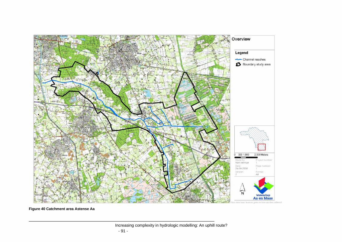
Increasing complexity in hydrologic modelling: An uphill route? - 91 -
Figure 40 Catchment area Astense Aa

Increasing complexity in hydrologic modelling: An uphill route? - 92 -
Figure 41 Digital elevation map

Increasing complexity in hydrologic modelling: An uphill route? - 93 -
Figure 42 Meteorological recording stations

Increasing complexity in hydrologic modelling: An uphill route? - 94 -
Figure 43 Measurement locations (selected measurements locations in green)

Increasing complexity in hydrologic modelling: An uphill route? - 95 -
Figure 44 Groundwater withdrawals

Increasing complexity in hydrologic modelling: An uphill route? - 96 -
6 Result calibration after optimization parameter values
Jan98 Jan99
0
1
2
3
4
5
6x 10
5 Q
Time
Dis
char
ge [m
3/da
y]
Measurementstap 0step 1step 2step 3step 4

Increasing complexity in hydrologic modelling: An uphill route? - 97 -
Apr97 Oct97 Apr98 Oct98 Apr9919.5
20
20.5
21
21.5
22
22.5
23H0199
Time
Hea
d [m
]
Measurementstep 1step 2step 3step 4
Apr97 Oct97 Apr98 Oct98 Apr9922
22.5
23
23.5
24
24.5C0241
Time
Hea
d [m
]
Apr97 Oct97 Apr98 Oct98 Apr9927.5
28
28.5
29
29.5
30
30.5C0422
Time
Hea
d [m
]
Apr97 Oct97 Apr98 Oct98 Apr9928
28.5
29
29.5
30
30.5C0508
Time
Hea
d [m
]
Apr97 Oct97 Apr98 Oct98 Apr9929.5
30
30.5
31
31.5D0154
Time
Hea
d [m
]

Increasing complexity in hydrologic modelling: An uphill route? - 98 -
7 Results step 1 to 2 exchange
Apr00 Jul00 Oct00 Jan01 Apr010
0.2
0.4
0.6
0.8
1
1.2
1.4
1.6
1.8
2x 10
5
Time [date]
Dis
char
ge [m
3/da
y]
Comparison exchange between domains
Discharge to river cells in step 1Discharge from channel flow to groundwater in step 2Discharge from groundwater to channel flow in step 2

Increasing complexity in hydrologic modelling: An uphill route? - 99 -
8 Results 2 to 3 separated
Apr00 Jul00 Oct00 Jan01 Apr010
0.5
1
1.5
2
2.5
3
3.5
4x 10
5 Q
Time
Dis
char
ge [m
3/da
y]
Measurementstep 2step 2 incl. faultstep 2 incl. fault and conductivitystep 3step 3 with low resistance

Increasing complexity in hydrologic modelling: An uphill route? - 100 -
Apr00 Jul00 Oct00 Jan01 Apr0119.5
20
20.5
21
21.5
22
22.5
23H0199
Time
Hea
d [m
]
Measurementstep 2step 2 incl faultstep 2 incl fault and conductivitystep 3step 3 with low resistance
Apr00 Jul00 Oct00 Jan01 Apr0122
22.5
23
23.5
24
24.5C0241
Time
Hea
d [m
]
Apr00 Jul00 Oct00 Jan01 Apr0127.5
28
28.5
29
29.5C0422
Time
Hea
d [m
]
Oct00 Jan01 Apr0128.6
28.8
29
29.2
29.4
29.6
29.8
30C0508
Time
Hea
d [m
]
Apr00 Jul00 Oct00 Jan01 Apr0129
29.5
30
30.5
31
31.5D0154
Time
Hea
d [m
]

Increasing complexity in hydrologic modelling: An uphill route? - 101 -
9 Results step 2 to 3 with extra layer
Apr00 Jul00 Oct00 Jan01 Apr0119.5
20
20.5
21
21.5
22
22.5
23H0199
Time
Hea
d [m
]
Measurementstep 2step 2 with extra layerstep 3 with extra layerstep 3step 3 with low resistance
Apr00 Jul00 Oct00 Jan01 Apr0122.5
23
23.5
24
24.5C0241
Time
Hea
d [m
]
Apr00 Jul00 Oct00 Jan01 Apr0128
28.2
28.4
28.6
28.8
29
29.2C0422
Time
Hea
d [m
]
Oct00 Jan01 Apr0128.6
28.8
29
29.2
29.4
29.6
29.8
30C0508
Time
Hea
d [m
]
Apr00 Jul00 Oct00 Jan01 Apr0129
29.5
30
30.5
31
31.5D0154
Time
Hea
d [m
]

Increasing complexity in hydrologic modelling: An uphill route? - 102 -
10 Discussion using groundwater recharge instead of precipitation - calibration results
Jan98 Jan990
1
2
3
4
5
6x 10
5 Q
Time
Dis
char
ge [m
3/da
y]
Measurementstep 1step 1 groundwater recharge

Increasing complexity in hydrologic modelling: An uphill route? - 103 -
Apr97 Oct97 Apr98 Oct98 Apr9919.5
20
20.5
21
21.5
22
22.5
23H0199
Time
Hea
d [m
]
Measurementstep 1step 1 groundwater recharge
Apr97 Oct97 Apr98 Oct98 Apr9920.5
21
21.5
22
22.5
23
23.5
24C0241
Time
Hea
d [m
]
Apr97 Oct97 Apr98 Oct98 Apr9927
27.5
28
28.5
29
29.5
30
30.5C0422
Time
Hea
d [m
]
Apr97 Oct97 Apr98 Oct98 Apr9928
28.5
29
29.5
30
30.5C0508
Time
Hea
d [m
]
Apr97 Oct97 Apr98 Oct98 Apr9928.5
29
29.5
30
30.5
31
31.5D0154
Time
Hea
d [m
]

Increasing complexity in hydrologic modelling: An uphill route? - 104 -
11 Discussion channel flow module
Figure 45 Discharge at several locations in the catchment
Apr00 Jul00 Oct00 Jan01 Apr010
0.5
1
1.5
2
2.5
3
3.5
4x 10
5 Q
Time
Dis
char
ge [m
3/da
y]
Measurementstap 1step 2(outlet)berkenAstense Aa (upper)Soeloop