Modeling and simulation of wireless sensor networks · scientifiques de niveau recherche, publiés...
215
HAL Id: tel-00690466 https://tel.archives-ouvertes.fr/tel-00690466 Submitted on 23 Apr 2012 HAL is a multi-disciplinary open access archive for the deposit and dissemination of sci- entific research documents, whether they are pub- lished or not. The documents may come from teaching and research institutions in France or abroad, or from public or private research centers. L’archive ouverte pluridisciplinaire HAL, est destinée au dépôt et à la diffusion de documents scientifiques de niveau recherche, publiés ou non, émanant des établissements d’enseignement et de recherche français ou étrangers, des laboratoires publics ou privés. Modeling and simulation of wireless sensor networks Wan Du To cite this version: Wan Du. Modeling and simulation of wireless sensor networks. Other. Ecole Centrale de Lyon, 2011. English. <NNT : 2011ECDL0026>. <tel-00690466>
Transcript of Modeling and simulation of wireless sensor networks · scientifiques de niveau recherche, publiés...

HAL Id: tel-00690466https://tel.archives-ouvertes.fr/tel-00690466
Submitted on 23 Apr 2012
HAL is a multi-disciplinary open accessarchive for the deposit and dissemination of sci-entific research documents, whether they are pub-lished or not. The documents may come fromteaching and research institutions in France orabroad, or from public or private research centers.
L’archive ouverte pluridisciplinaire HAL, estdestinée au dépôt et à la diffusion de documentsscientifiques de niveau recherche, publiés ou non,émanant des établissements d’enseignement et derecherche français ou étrangers, des laboratoirespublics ou privés.
Modeling and simulation of wireless sensor networksWan Du
To cite this version:Wan Du. Modeling and simulation of wireless sensor networks. Other. Ecole Centrale de Lyon, 2011.English. <NNT : 2011ECDL0026>. <tel-00690466>

ECOLE CENTRALE DE LYON
ECOLE DOCTORALE Electronique, Electrotechnique, Automatique
Institut des Nanotechnologies de Lyon
Annee : 2011 These Numero : 2011-26
Thesepour obtenir le grade de
DOCTEUR DE L’ECOLE CENTRALE DE LYON
Discipline : Electronique
presentee et soutenue par
Wan DU
le mercredi 14 septembre 2011
Modelisation et Simulation de Reseaux de
Capteurs sans Fil
These dirigee par Ian O’CONNOR
JURY :
Lionel TORRES Professeur, Universite Montpellier 2 PresidentHerve GUYENNET Professeur, Universite de Franche-Comte RapporteurCecile BELLEUDY Maıtre de Conferences, Universite de Nice-Sophia Antipolis Rapporteur
Fabien MIEYEVILLE Maıtre de Conferences, Ecole Centrale de Lyon Examinateur
David NAVARRO Maıtre de Conferences, Ecole Centrale de Lyon Examinateur
Ian O’CONNOR Professeur, Ecole Centrale de Lyon Examinateur


To my parents and my sister

Acknowledgements
I would like to express my sincere appreciation to Prof. Ian O’connor, Dr. David
Navarroc and Dr. Fabien Mieyeville for their supervision, guidance and support
throughout my Ph.D. I am grateful to them for having shared so much of time and
insight in our weekly discussions. I have learned a lot from them.
I would also like to thank the China Scholarship Council (CSC) for the financial
support of my Ph.D studies. I am also thankful for the research facilities and support
provided by the Lyon Institute of Nanotechnology and Ecole Centrale de Lyon. I am also
grateful to the heterogeneous systems design group for providing travel support in order
for me to publish and present my research in many international conferences.
I wish to thank my colleagues of the heterogeneous systems design group, including
Junchen Liu who guided me for the work and life at Lyon when I first arrived in France,
Felipe Frantz, Vijayaragavan Viswanathan, Mihai Galos, Kotb Jabeur, Lioua Labrak,
Nataliya Yakymets, Zhenfu Feng and Nanhao Zhu who are always willing to share their
knowledge with me and have made it such an interesting place to work over the past
three years. I would also like to thank the two excellent engineers, Laurent Carrel and
Raphael Lopez, for their technical supports of my research. Moreover, I won’t forget the
help from the secretaries, Ms. Patricia Dufaut and Ms. Nicole Durand, for their kindness,
availability and good humor that ease my thesis life.
Finally, I wish to thank my family and friends. Without their love and support, I can
never complete this thesis.

Resume en francais (Abstract in French)
Les evolutions des technologies du microsysteme electromecanique (MEMS) et de
l’integration a tres grande echelle (VLSI) ont facilite le developpement de capteurs
intelligents et de microprocesseurs et transceivers radiofrequence a faible puissance,
permettant l’essor des reseaux de capteurs sans fil (WSN: Wireless Sensor Networks)
ces dernieres annees. Un nœud de reseau de capteurs est generalement equipe d’un ou
plusieurs capteurs, une unite de calcul, une memoire, une alimentation et d’une frequence
radio (RF) transceiver. Divers phenomenes peuvent etre mesures, tels que les sons,
vibrations, humidite, pression ou temperature.
Les WSN ont ete utilises dans une large variete d’applications. Selon leurs
fonctionnalites, les applications peuvent etre essentiellement classees en deux categories:
les applications de surveillance et les applications de suivi. Diverses applications ont des
exigences differentes; par exemple, une application industrielle en temps reel necessite
une latence faible de livraison de paquets, mais une autonomie d’une semaine est souvent
suffisante. En revanche, un systeme de surveillance de l’environnement a distance devra
avoir une duree de vie de plusieurs annees avec un rapport cyclique faible. En raison de la
petite taille et des exigences de faible cout des nœuds, les ressources de nœuds de capteurs
telles que la capacite de traitement, le stockage et l’energie, sont limites.
Pour mettre en œuvre de nouvelles applications, les techniques de reseau devraient
etre etudiees afin de transmettre les donnees d’un nœud a un hote qui peut etre consulte
par les utilisateurs. Les protocoles de communication des reseaux de capteurs peuvent
etre representes en differentes couches, comme la couche d’application, de transport, de
reseau, de liaison de donnees et de physique. Chaque couche a plusieurs taches specifiques
et fournit des services a sa couche superieure. Trois caracteristiques particulieres rendent
la conception de protocoles WSN differents des autres reseaux sans fil (par exemle
informatiques). Un exeple est la source d’alimentation limitee qui necessite des protocoles
WSN dedies a l’economie d’energie. Le dernier est le deploiement a grande echelle. Dans

un reseau compose de centaines ou de milliers de nœuds de capteurs, l’hote peut etre situe
hors de la portee de transmission de certains nœuds, ce qui necessite la communication
multi-sauts (multi-hop).
Pour repondre aux diverses exigences des applications WSN, les concepteurs ont besoin
d’envisager un grand nombre de choix de conception au niveau du nœud (par exemple,
la consommation d’energie des composants materiels et la capacite de traitement) et de
nombreux parametres au niveau du protocole (par exemple, les algorithmes d’anti-collision
et des methodes de routage). Comparee aux mesures sur banc de test, la simulation est
un moyen economique et rapide pour explorer de nombreuses solutions. La simulation est
actuellement la methode la plus largement adoptee pour analyser les reseaux de capteurs.
En raison de l’energie limitee sur les nœuds de capteurs, et afin de prolonger la duree
de vie du reseau, de nombreux efforts ont ete efectues pour reduire la consommation
d’energie du materiel, du logiciel, du protocole de communication et de l’application.
Par consequent, il est necessaire de prevoir avec precision la consommation d’energie des
WSN, qui exige des modeles detailles du materiel et du logiciel (HW/SW) des nœuds de
capteurs.
Beaucoup d’outils de simulation de WSN ont ete developpes en utilisant des
methodes differentes telles que la simulation generale du reseau, l’emulation du systeme
d’exploitation (OS), la simulation d’instructions, et la simulation niveau systeme (SLDL).
Cependant, la plupart d’entre eux sont mis en œuvre dans les langages de programmation
generiques comme C++ et Java qui ne supportent pas directement la co-simulation
de HW/SW. Seul un petit nombre de simulateurs concus en SLDLs supportent la
modelisation de la concurrence, de l’interruption et des primitives de synchronisation des
systemes embarques. Par exemple, SystemC est une bibliotheque en C++ qui permet la
conception d’un systeme materiel et logiciel. Il permet de modeliser le systeme embarque
a differents niveaux d’abstraction et permettent aux concepteurs de se concentrer sur les
fonctionnalites du systeme en masquant les details de communication et de calcul.
Par consequent, afin de permettre la co-simulation materielle / logicielle (HW/SW)

des nœuds et l’estimation precise de la consommation d’energie des reseaux de capteurs, la
faisabilite et les avantages de l’utilisation de SLDLs dans la modelisation et la conception
de reseaux de capteurs sans fil doivent etre etudies. Un simulateur en SLDL pour les
WSN devrait etre valide par des mesures experimentales et evalue en comparant avec les
autres simulateurs existants de WSN.
Un simulateur de WSN en SystemC, nommee IDEA1 (hIerarchical DEsign plAtform
for sensOr Networks Exploration) a ete developpe. IDEA1 permet l’evaluation rapide
des performances d’un WSN au niveau systeme. Les resultats des simulations incluent le
taux de livraison de paquets (PDR: Packet Delivery Rate), la latence de transmission et la
consommation d’energie. La principale caracteristique d’IDEA1 est la prediction precise
de la consommation d’energie. Le modele d’energie mis en œuvre dans IDEA1 prend
en compte les consommations de puissance de tous les modes operationnels de chaque
composant materiel et les transitions entre ces differents modes.
Plusieurs plateformes de WSN, telless que MICAz et MICA2, sont modelises. La
norme IEEE 802.15.4 est mise en œuvre. IEEE 802.15.4 a ete largement utilise dans
les applications de WSN, car il est concu pour les communications bas debit et pour les
applications a faible consommation d’energie en conformite avec les contraintes des WSN.
Quatre simulateurs de WSN en SystemC ont ete developpes, mais IDEA1 est le premier
simulateur en SystemC de WSN qui a ete valide avec des mesures experimentales et evalue
en comparant avec d’autres simulateurs. La validation des modeles de simulation est
necessaire pour obtenir une precision suffisante et connue.LA comparaison avec d’autres
simulateurs peuvent evaluer les performances de IDEA1, principalement par rapport aux
aspects reseau.
Les contributions principales de cette these sont les quatre parties suivantes:
• Conception d’IDEA1: C’est un environnement de conception et de simulation
systeme pour les WSN. Il est developpe en SystemC. L’architecture d’IDEA1 est
modulaire, donc de nouveaux modules (composants) peuvent etre facilement mis
en œuvre et rajoutes. Beaucoup de parametres au niveau systeme du nœud et au

niveau du reseau peuvent etre configures.
• Validation et evaluation d’IDEA1: Un banc d’essai de 9 nœuds de capteurs a ete
construit pour valider les resultats de simulation d’IDEA1. Les simulations d’IDEA1
ont egalement ete comparees avec NS-2, le simulateur le plus utilise dans le domaine
des reseaux mobiles ad hoc (MANET). Les parametres compares sont la precision
de la simulation, l’analyse de la consommation et la vitesse de la simulation.
• Etude du reseau de capteurs IEEE 802.15.4: La performance d’un reseau de capteurs
IEEE 802.15.4 est etudie par IDEA1, y compris les taux de livraison de paquets,
la latence moyenne, la consommation d’energie par paquets et la consommation
moyenne de puissance. De nombreux cas avec differentes configurations des
parametres du protocole sont simules.
• Etude d’une application industrielle: Dans ce projet, un reseau de capteurs sans fil
est deploye sur un vehicule pour mesurer les vibrations. Par la simulation d’IDEA1,
certaines conceptions preliminaires basees sur des protocoles de communication et
des plates-formes materielles sont evaluees.
Cette these est organisee comme suit. Le chapitre 2 presente les reseaux de capteurs
sans fil par rapport aux applications, aux plates-formes materielles, aux protocoles de
communication, a la modelisation et a la simulation. Une taxonomie des outils de
simulation WSN est proposee. L’etat de l’art des simulateurs existants de WSN est resume
selon le schema de classification de la taxonomie. Le chapitre 3 decrit la conception
d’IDEA1. L’architecture, la mise en œuvre du modele de simulation, les sorties, la
modelisation du reseau, et le modele d’energie sont expliques en detail. Le chapitre 4
valide les resultats de la simulation et evalue la performance d’IDEA1. Les resultats de
simulation d’IDEA1 sont compares avec certaines mesures experimentales sur un banc
d’essai de 9 nœuds. Les performances d’IDEA1 ont egalement ete compares avec NS-2, le
simulateur le plus largement utilise dans la recherche sur les WSN. Le chapitre 5 utilise
deux cas d’etudes pour montrer le flot de conception d’IDEA1. La performance du reseau

IEEE 802.15.4 du capteur est globalement evaluee. En outre, IDEA1 est egalement utilise
pour etudier une application industrielle dans lequel un reseau de capteur sans fil est
deploye sur un vehicule pour mesurer les vibrations. Le chapitre 6 conclut cette these et
decrit des perspectives interessantes.
Chapitre 2 Introduction au Reseau de Capteur sans Fil
Les reseaux de capteurs sans fil (WSN) sont des reseaux ad hoc de nœuds aux
ressources limitees qui sont deployes a differents endroits pour surveiller les conditions
physiques ou environnementales, comme la temperature, la vibration et le mouvement. Ce
sont des reseaux uniques en raison de ressources limitees (capacite de memoire, de calcul
et d’energie). Comme les nœuds sont souvent concus pour fonctionner sur des periodes de
plusieurs mois ou annees, l’energie est la ressource la plus precieuse des nœuds. WSN ont
ete employes dans beaucoup d’applications, tels que la surveillance de l’environnement,
les applications militaires et industrielles [1]. Differentes applications ont des exigences
differentes sur le materiel de capteur et les protocoles du reseau. La modelisation et
simulation ont ete largement utilisees pour evaluer la performance des systemes de WSN.
Dans la section 2.1, les applications de WSN sont introduites. Dans un passe recent,
les WSNs ont trouve leur place dans une grande variete d’applications. Comme dans le
systeme de classification dans [2], les applications de WSN peuvent etre essentiellement
classees en deux categories: les applications de surveillance et les applications de suivi.
Dans les applications de surveillance, des reseaux de capteurs sont deployes dans un
endroit pour surveiller les phenomenes. Dans les applications de suivi, un ou plusieurs
nœuds de capteurs sont attaches a un objet cible et une infrastructure de reseau
de capteurs est deployee afin de detecter le mouvement de cet objet ou suivre ses
caracteristiques.
Dans la section 2.2, les plateformes materielles actuelles disponibles sont etudiees.
Un nœud est normalement compose d’un ou plusieurs capteurs, une unite de traitement,
un transceiver radiofrequence(RF) et une ou plusieurs sources d’energie. En plus de
la mesure, un nœud a besoin pour traiter les donnees d’une unite de traitement,

de transmettre les informations a d’autres nœuds grace a son transceiver RF, en
consommmant le moins d’energie de la batterie.
Dans la section 2.3, l’architecture du reseau et les protocoles de communication sont
analyses. LA couche MAC (Medium Access Control) definit les procedures de l’acces
au canal, afin d’eviter les corruptions de donnees et les collisions de paquets. Il assure
la fiabilite de la transmission entre deux nœuds en utilisant certaines retransmissions,
comme les accuses de reception (ACK). De plus, il detecte et corrige eventuellement les
erreurs qui peuvent survenir dans la couche inferieure.
Dans la section 2.4, les systemes d’exploitation de WSN sont etudies. Beaucoup
d’aspects essentiels de ces systemes d’exploitation t sont resumes, y compris les
plateformes materielles prises en charge, les langages de programmation, et la
reprogrammation.
Dans la section 2.5, une taxonomie des simulateurs existants de WSN est proposee. Il
partage les outils de simulation en quatre categories selon leurs methodes de modelisation.
Basee sur le systeme de classification de la taxonomie, une analyse sur les outils
existants de simulation est presentee. Base sur l’analyse ci-dessus d’outils existants de
simulation de WSN, nous pouvons constater que la plupart des simulateurs sont mis
en œuvre dans les langages de programmation generiques comme C++ et Java qui ne
supportent pas directement la co-simulation du materiel et du logiciel de nœud. Les
simulateurs generiques de reseau se concentrent principalement sur l’etude des protocoles
de communication. Les emulateurs du systeme exploitation et les ISS (instruction set
simulator) peuvent accelerer la mise en œuvre du logiciel embarque, mais elles impliquent
beaucoup de details au bas niveau qui ne sont pas forcement disponibles au stade de la
conception. Les simulations a ce niveau ont normalement besoin d’une implementation
executable de l’application finale et les protocoles. Seul un petit nombre de simulateurs
concus dans SLDLs, tels que SystemC, peuvent fournir l’abstraction appropriee du
systeme final, mais aussi avec assez d’information detaillee sur le materiel et les operations
du logiciel. En outre, la modelisation en SLDL est compatible avec le flot de conception

microelectrique.
SystemC fournit un support natif de modelisation simultanee, la hierarchie
structurelle, les interruptions et les primitives de synchronisation des systemes
embarques [3]. Beneficiant de la co-simulation de HW/SW, SystemC est plus approprie
pour la modelisation et simulation de WSN. A l’heure actuelle, quatre simulateurs en
SystemC de WSN [4, 5, 6, 7] ont ete developpes, mais aucun d’eux n’a ete valide avec des
mesures experimentales ou evalues globalement en comparant avec d’autres simulateurs.
Pour resoudre cette limitation, un nouveau simulateur en SystemC de WSN nommee
IDEA1 (plateforme de conception hierarchique de reseaux de capteurs Exploration) a
ete developpe. Un banc d’essai de 9 nœuds a ete construit pour valider les resultats de
simulation d’IDEA1. Les simulations d’IDEA1 ont egalement ete compares avec NS-2 qui
est le simulateur le plus utilise dans la recherche de WSN mobile ad hoc (MANET) [8].
Chapitre 3 Conception et Implementation d’IDEA1
Dans ce chapitre, un nouveau simulateur de WSN, nomme IDEA1 (hIerarchical DEsign
plAtform for sensOr Networks Exploration), est presente. Les nœuds sont modelises en
SystemC et leurs interconnexions en C++. SystemC est un langage de description niveau
systeme qui est largement utilise dans la conception du systeme sur puce, par consequent,
IDEA1 n’est pas seulement un simulateur, mais aussi un outil de conception de systemes
pour WSN. Avec un modele du nœud de capteur, il est possible d’evaluer la performance
du reseau. Quand les exigences du systeme final sont remplies, la mise en œuvre reelle de
la conception du systeme peut commencer a partir de cette description. IDEA1 fournit
aux concepteurs de systemes des possibilites d’evaluer la performance du reseau avec
de nouvelles architectures a un stade precoce, et il permet egalement aux concepteurs de
simuler le protocole de communication sur des nouveaux nœuds, meme si les plates-formes
materielles sont encore en developpement.
La section 3.1 presente brievement SystemC. SystemC est une bibliotheque en C++
pour la conception du materiel et du systeme. Il peut etre utilise par les concepteurs
de systemes complexes materiels et logiciels (HW/SW) [9]. Il supporte la co-design du

HW/SW a un niveau eleve d’abstraction. Cette evaluation de la performance primaire
donne au concepteur une comprehension fondamentale du systeme final a un stade precoce
du processus de conception.
La section 3.2 decrit l’architecture d’IDEA1. IDEA1 est un outil de simulation.
Chaque composant est modelise comme un module individuel en SystemC qui
communique avec les autres via les canaux. Le noyau SystemC agit comme moteur de
simulation. Il planifie l’execution des processus et des mises a jour de l’etat de tous
les modules a chaque cycle de simulation. Tous les processus actifs sont invoques au
meme moment, ce qui cree une illusion de simultaneite. Les nœuds de capteurs sont
modelises exactement comme leurs architectures. Les composants materiels d’un nœud de
capteur comprennent generalement un microcontroleur, un transceiver, plusieurs capteurs
et une batterie. Chaque composante est modelisee comme un module individuel de
SystemC. IDEA1 comprend une bibliotheque qui contient de nombreuses implementations
de plateformes materielles existantes et de protocoles de communication. Il fournit
egalement un environnement graphique pour permettre aux utilisateurs une configuration
simple de la simulation et l’analyse des resultats.
La section 3.3 illustre la mise en œuvre d’IDEA1. Le microcontroleur et le transceiver
RF sont modelises comme des machines d’etats finis (FSM). La FSM du microcontroleur
est controlee par les interruptions generees par le transceiver et l’application. La transition
de l’etat de transceiver est declenchee par trois types d’evenements, y compris le protocole
mis en œuvre, les commandes du microcontroleur et les evenements reseau. Le modele de
reseau relie chaque nœud, gere la topologie du reseau et mise en œuvre de la propagation
des ondes radio. Le modele de reseau etablit un eventail de topologie a deux dimensions
base sur cette information et les modeles de propagation radio. Dans IDEA1, chaque
etat des composants materiels principaux dans un nœud de capteur est associe a une
consommation de courant. La duree et la consommation instantanee de chaque transition
entre deux etats sont egalement identifiees. Pendant la simulation, les etats de ces
composants sont mis a jour en fonction de l’execution des logiciels et des evenements

du reseau.
La section 3.4 presente les resultats de la simulation. Il y a deux types de sortie
de simulation dans IDEA1, y compris le log de simulation et le chronogramme des
evenements. Le log de simulation est utilise pour deboguer les implementations du
modele et montrer les comportements du reseau. Beaucoup de resultats statistiques des
comportements du reseau sont donnes a la fin du log de simulation, y compris les aspects
debit, latence de livraison de paquets, consommations de puissance et temps de simulation.
Pendant que la simulation est en cours, les etats de tous les composants materiels et les
variables sont mises a jour en permanence et suivis dans un fichier (VCD), et peuvent
etre affichees graphiquement en utilisant des outils de visualisation de forme d’onde.
Dans ce chapitre, un nouveau simulateur WSN niveau systeme, nomme IDEA1, est
presente. Il est developpe en SystemC et C++, ce qui rend la simulation compatible
au flot de conception des systemes embarques. Il permet l’exploration de l’espace de
conception a un stade precoce et permet une modelisation modulaire de nœuds de capteurs
et d’applications de WSN. Beaucoup de plateformes materielles ont ete modelisees et la
norme IEEE 802.15.4 a ete mise en œuvre. Un modele d’energie a ete propose pour tous
les modeles de composants d’IDEA1.
Chapitre 4 Validation et Evaluation d’IDEA1
Dans ce chapitre, les performances d’IDEA1 sont evaluees, en particulier sous deux
aspects: la precision et le temps de simulation. Pour la validation de la precision, les
resultats de simulation d’IDEA1 sont compares avec des mesures sur un banc d’essai
compose de 9 nœuds. La simulation d’IDEA1 est egalement comparee avec NS-2, le
simulateur le plus largement utilise dans la recherche des WSN, y compris les comparaisons
des resultats de simulation et le temps de simulation.
La section 4.1 presente les parametres utilises pour evaluer les performances du
reseau. Quatre indicateurs sont utilises pour evaluer les performances du reseau dans
les experiences et les comparaisons avec NS-2, dont le taux de delivrance des paquets
(PDR), le temps de latence moyen (AL), la consommation d’energie par paquet (ECPkt)

et la consommation electrique moyenne (APC ).
La section 4.2 decrit le banc d’essai et montre la comparaison entre les mesures et
les resultats de simulation. Un banc d’essai de 9 nœuds est construit. Deux types de
mesures ont ete effectues. L’une est la mesure des consommations de tous les modes de
fonctionnement d’un nœud afin de calibrer le modele d’energie, qui sera utilisee dans la
simulation d’IDEA1. L’autre est la mesure sur le banc d’essai du reseau de 9 nœuds. Ce
reseau se compose de huit nœuds et un coordinateur. Les nœuds sentent l’environnement
periodiquement. La frequence de lecture est presentee comme le taux d’echantillonnage.
L’application realisee avec le banc d’essai a egalement ete mis en œuvre dans IDEA1 avec la
meme configuration. Pour evaluer les performances du reseau avec des rapports cycliques
differents, et la periode d’echantillonnage est fixe a 10, 1, 0,1, 0,01 et 0,001 secondes
respectivement. La deviation moyenne des quatre metriques (PDR, AL, APC et ECPkt)
entre les simulations et les mesures est de 5,2%, 3,2%, 3,4% et 6,5% respectivement. Par
consequent, la deviation moyenne entre les simulations et les mesures est de 4,6% qui peut
etre accepte pour les simulations generaux au haut niveau.
La section 4.3 presente les resultats de simulation d’IDEA1 et de NS-2 sur un reseau
utilisant IEEE 802.15.4. De nombreux cas avec differentes configurations (principalement
BO et SO) et des taux d’echantillonnage ont ete evalues. Des parametres de l’algorithme
CSMA-CA (par exemple, macMinBE, macMaxCSMABackoffs, macMaxFrameRetries,
etc) sont definis avec les valeurs par defaut de la norme IEEE 802.15.4. Trois types
de resultats de simulation sont compares, y compris NS-2, IDEA1 avec la modelisation du
materiel (IDEA1_ HW) et IDEA1 sans la modelisation du materiel (IDEA1_ NOHW).
Dans la derniere simulation, tous les parametres materiels sont mis a 0. Comme le modele
IEEE 802.15.4 de NS-2 ne considere pas le materiel, NS-2 et IDEA1_ NOHW sont au
meme niveau d’abstraction. La deviation moyenne entre les IDEA1_ HW et NS-2 est de
26,7%, et celui entre IDEA1_ NOHW et NS-2 est de 4,8%. Le premier est plus grand
puisque l’information plus detaillee des operations HW/SW a ete consideree. La vitesse
de simulation des IDEA1 est 2 fois plus rapide que NS-2.

Chapitre 5 Cas d’etudes
Apres la validation experimentale de la precision et l’evaluation des performances,
IDEA1 est pret a etre utilise dans des applications reelles. Il est d’abord utilise pour fournir
l’evaluation du reseau IEEE 802.15.4 etudie dans le dernier chapitre. Les performances
d’IEEE 802.15.4 sont evaluees pour differents parametrages. Enfin, IDEA1 est utilise pour
etudier une application industrielle. Par la simulation, certaines conceptions preliminaires
bases sur les protocoles IEEE 802.15.4 et deux plates-formes materielles differentes ont
pu etre evaluees. Les quatre parametres utilises dans le chapitre 4, y compris les PDR,
AL, ECPkt et APC, sont evalues.
La section 5.1 propose une evaluation des performances du reseau IEEE 802.15.4 par
NS-2 et IDEA1. Selon l’etude dans la section 4.3, lorsque le taux d’echantillonnage est
petit, les nœuds depensent trop d’energie pour la recherche du paquet (traking) beacon.
Par consequent, dans cette section, nous mettons en œuvre la meme application, sans
tracking. Jusqu’a present, BO est regle sur 0, 1 et 2 respectivement, et SO est mis a 0.
Certaines autres configurations des parametres du protocole et du mode non-beacon sont
egalement evalues pour trouver le meilleur choix de l’algorithme et la configuration des
parametres pour des echantillonnages differents.
La section 5.2 etudie une application industrielle pour demontrer le flot de conception
et de la convivialite d’IDEA1. Un reseau de capteurs et actionneurs sans fil est deploye sur
une automobile pour mesurer et controler ses vibrations. La premiere tache de notre travail
est de concevoir le reseau de capteurs. Au debut, certains concepts preliminaires bases sur
plusieurs plates-formes materielles et protocoles existantes doivent etre examinees. Quatre
algorithmes MAC sont mises en œuvre, y compris IEEE 802.15.4 unslotted CSMA-CA,
IEEE 802.15.4 slotted CSMA-CA, IEEE 802.15.4 GTS et TDMA GTS. Deux plates-
formes materielles ont ete utilisees, N@L et MICAz.
Les algorithmes de CSMA-CA ne sont pas appropries pour cette application en raison
du faible PDRs, qui est du au grand nombre de collisions. Le systeme se sature quand
le taux d’echantillonnage est trop eleve. Le PDR de l’IEEE 802.15.4 GTS est grand,
mais la latence est egalement tres grande. Pour l’algorithme TDMA GTS, le PDR peut
atteindre 100%, mais ce reseau IEEE 802.15.4 ne peut pas repondre a l’exigence en temps
reel de cette application. Bien que la latence moyenne des paquets peut atteindre 7,0 ms,
le sizePayload est de 10 echantillons qui signifie que le premier echantillon de donnees
doit attendre au moins 17 ms avant d’etre recus par le coordonnateur. Cette latence
des donnees de capteurs est trop elevee pour generer un controle actif en temps reel.
Par consequent, nous avons conclu que la norme IEEE 802.15.4 ne peut pas repondre a
l’exigence de cette application. Certains protocoles de communications a haute vitesse
doivent etre etudies.
Chapitre 6 Conlusions et Perspectives
Cette these a etudie la modelisation et la simulation de reseaux de capteurs sans fil.
Un nouveau simulateur WSN, nomme IDEA1, a ete developpe en SystemC.
Base sur le support de la concurrence par SystemC, la hierarchie structurelle, les
interruptions et les primitives de synchronisation, IDEA1 permet la co-simulation du
materiel et du logiciel des nœuds. En effet, les consommations d’energie d’un nœud
individuel de capteurs et du reseau peuvent etre predites avec precision. Le modele
d’energie mis en œuvre dans IDEA1 prend en compte les consommations de puissance
de tous les modes de fonctionnement de chaque composant materiel et les transitions
entre les differents modes. Beaucoup de composants materiels, comme ceux composant
les plateformes MICAz et MICA2, sont modelises. La norme IEEE 802.15.4 a ete mise en
œuvre.
Premierement, les resultats de simulation d’IDEA1 ont ete compares avec des mesures
experimentales sur un banc d’essai de 9 nœuds, sur les aspects de taux de livraison
de paquets, latence moyenne, consommation d’energie par paquets et consommation
moyenne de puissance. La deviation moyenne entre les simulations d’IDEA1 et les mesures
experimentales est de 4,6% qui peut etre accepte pour une simulation au niveau systeme.
Les performances d’IDEA1 ont egalement ete comparees avec NS-2, le simulateur reseau
le plus largement utilise dans la recherche de WSN. Beneficiant de modeles materiels et

logiciels, IDEA1 fournit des informations plus detaillees sur les consommations d’energie
que NS-2. Si les informations de certaines operations materielles relatives ne sont pas
prises en compte dans IDEA1, la deviation moyenne entre les simulations d’IDEA1 et
de NS-2 est de 4,8% ce qui prouve qu’IDEA1 peut fournir la meme precision avec NS-
2. Toutefois, si les operations materielles relatives sont considerees dans la simulation
d’IDEA1, la deviation moyenne entre les simulations d’IDEA1 et NS-2 est de 26,7%. La
vitesse de simulation d’IDEA1 est 2 fois plus vite que NS-2.
Enfin, deux cas d’etudes ont ete realises pour montrer la facilite d’utilisation et le flot de
conception d’IDEA1. La performance du reseau IEEE 802.15.4 a ete entierement evaluee.
Pour differentes charges de trafic, differents parametres des protocoles sont simules. En
outre, une application temps reel de controle actif des vibrations a egalement ete etudiee.
Par les etudes de simulation d’IDEA1, le meilleur choix de protocole de communication
bases sur MICAz ou N@L a ete trouve.
Les travaux de recherche mis en œuvre dans cette these ont montre des resultats
interessants. Toutefois, il y a beaucoup de recherches supplementaires qui pourraient etre
menees.
• Pour renforcer la capacite d’IDEA1 dans la modelisation des systemes reels de WSN,
certains capteurs doivent etre modelises en SystemC.
• Le systeme d’exploitation est une partie importante du developpement de logiciels
pour le systeme de WSN, par consequent IDEA1 sera plus complet si on peut
modeliser le systeme d’exploitation. En outre, des modeles precis du logiciel, telles
que la simulation de jeu d’instructions, peut etre etudiee.
• La simulation du reseau IEEE 802.15.4 a montre que cette norme est plus efficace
pour les applications a faible rapport cyclique. Donc, pour certaines applications
a haute frequence d’echantillonnage, les protocoles de communication haut debit
doivent etre etudies.
• Les couches hautes, comme des couches reseau et transport, devraient etre mises en

œuvre afin de permettre la simulation a grande echelle du reseau de capteurs.
• Les modeles de propagation radio dans la version actuelle d’IDEA1 ne contient
que deux modeles typiques. Certains modeles de propagation plus precis et plus
complexes doivent etre mises en œuvre dans IDEA1.
• Le modele de decharge de batterie dans la version actuelle d’IDEA1 est seulement
un processus lineaire. Certains modeles plus precis doivent etre etudies.

Contents I
Contents

II Contents

Contents III
Table of Contents . . . . . . . . . . . . . . . . . . . . . . . . . . . . . . I
List of Figures . . . . . . . . . . . . . . . . . . . . . . . . . . . . . . . . VIII
List of Tables . . . . . . . . . . . . . . . . . . . . . . . . . . . . . . . . . XIII
Chapter 1 : Introduction . . . . . . . . . . . . . . . . . . . . . 1
1.1 Brief Introduction to Wireless Sensor Networks . . . . . . . . . . . . . . . 3
1.2 Research Motivation . . . . . . . . . . . . . . . . . . . . . . . . . . . . . . 4
1.3 Research Contributions . . . . . . . . . . . . . . . . . . . . . . . . . . . . . 5
1.4 Selected Publications . . . . . . . . . . . . . . . . . . . . . . . . . . . . . . 6
1.5 Thesis Structure . . . . . . . . . . . . . . . . . . . . . . . . . . . . . . . . . 8
Chapter 2 : Wireless Sensor Networks . . . . . . . . . . 11
2.1 Application Scenarios . . . . . . . . . . . . . . . . . . . . . . . . . . . . . . 13
2.1.1 Monitoring Application Examples . . . . . . . . . . . . . . . . . . . 14
2.1.2 Tracking Application Examples . . . . . . . . . . . . . . . . . . . . 16
2.1.3 Summary . . . . . . . . . . . . . . . . . . . . . . . . . . . . . . . . 17
2.2 Wireless Sensor Hardware Platforms . . . . . . . . . . . . . . . . . . . . . 18
2.2.1 Architecture of wireless sensor node . . . . . . . . . . . . . . . . . . 18
2.2.2 Hardware platforms . . . . . . . . . . . . . . . . . . . . . . . . . . . 20
2.3 Communication Protocols . . . . . . . . . . . . . . . . . . . . . . . . . . . 20
2.3.1 Introduction to Protocol Stacks . . . . . . . . . . . . . . . . . . . . 22
2.3.2 Medium Access Control . . . . . . . . . . . . . . . . . . . . . . . . 24
2.3.2.1 Synchronous MAC Protocols . . . . . . . . . . . . . . . . 25
2.3.2.2 Asynchronous MAC Protocols . . . . . . . . . . . . . . . . 27
2.3.2.3 IEEE 802.15.4 MAC protocols . . . . . . . . . . . . . . . . 28
2.3.3 Data Aggregation and Routing . . . . . . . . . . . . . . . . . . . . 32
2.3.3.1 Network Topologies . . . . . . . . . . . . . . . . . . . . . 33
2.3.3.2 Routing Protocol for Mesh Topology . . . . . . . . . . . . 34

IV Contents
2.3.3.3 Routing Protocol for Cluster Topology . . . . . . . . . . . 35
2.4 Operating Systems . . . . . . . . . . . . . . . . . . . . . . . . . . . . . . . 36
2.4.1 Characteristics of WSN Operating Systems . . . . . . . . . . . . . . 36
2.4.2 Summary of WSN Operating Systems . . . . . . . . . . . . . . . . . 37
2.5 Modeling and Simulation . . . . . . . . . . . . . . . . . . . . . . . . . . . . 40
2.5.1 Requirements of WSN Modeling and Simulation . . . . . . . . . . . 41
2.5.2 A Typical Model of WSN System . . . . . . . . . . . . . . . . . . . 42
2.5.3 A Taxonomy of WSN Simulation Tools . . . . . . . . . . . . . . . . 43
2.5.4 A Survey of WSN Simulation Tools . . . . . . . . . . . . . . . . . . 45
2.5.4.1 Network Simulators with Node Models . . . . . . . . . . . 45
2.5.4.2 Node Emulators with Network Models . . . . . . . . . . . 49
2.5.4.3 Node System Simulator with Network Models . . . . . . . 51
2.5.4.4 Network Simulators with Node Emulators . . . . . . . . . 53
2.5.5 Summary . . . . . . . . . . . . . . . . . . . . . . . . . . . . . . . . 53
2.6 Conclusion . . . . . . . . . . . . . . . . . . . . . . . . . . . . . . . . . . . . 56
Chapter 3 : Design and Implementation IDEA1 . 57
3.1 Modeling Wireless Sensor Networks with SystemC . . . . . . . . . . . . . . 59
3.1.1 Introduction to SystemC . . . . . . . . . . . . . . . . . . . . . . . 59
3.1.1.1 Features of SystemC . . . . . . . . . . . . . . . . . . . . . 60
3.1.1.2 SystemC Modeling Constructs . . . . . . . . . . . . . . . . 60
3.1.1.3 SystemC Simulation Kernel . . . . . . . . . . . . . . . . . 61
3.1.2 Transaction Level Modeling . . . . . . . . . . . . . . . . . . . . . . 62
3.2 IDEA1 Framework . . . . . . . . . . . . . . . . . . . . . . . . . . . . . . . 63
3.2.1 Architecture of IDEA1 . . . . . . . . . . . . . . . . . . . . . . . . . 63
3.2.2 Design Flow of IDEA1 . . . . . . . . . . . . . . . . . . . . . . . . . 65
3.2.3 Current Library . . . . . . . . . . . . . . . . . . . . . . . . . . . . . 66
3.2.4 Graphical User Interface . . . . . . . . . . . . . . . . . . . . . . . . 71
3.2.5 IDEA1 Features . . . . . . . . . . . . . . . . . . . . . . . . . . . . . 72

Contents V
3.3 Simulation Model Implementations . . . . . . . . . . . . . . . . . . . . . . 74
3.3.1 Sensor Node Modeling . . . . . . . . . . . . . . . . . . . . . . . . . 74
3.3.2 Microcontroller Model . . . . . . . . . . . . . . . . . . . . . . . . . 75
3.3.2.1 Model of ATMEL ATMega128 . . . . . . . . . . . . . . . 80
3.3.2.2 Model of Microchip PIC16LF88 . . . . . . . . . . . . . . . 82
3.3.3 Transceiver Model . . . . . . . . . . . . . . . . . . . . . . . . . . . 85
3.3.3.1 Transceiver Model of TI CC2420 and CC1000 . . . . . . . 86
3.3.3.2 Transceiver Model of Microchip MRF24J40 . . . . . . . . 86
3.3.4 Network Modeling . . . . . . . . . . . . . . . . . . . . . . . . . . . 89
3.3.4.1 Packet Transmission . . . . . . . . . . . . . . . . . . . . . 90
3.3.4.2 Radio Propagation Model . . . . . . . . . . . . . . . . . . 90
3.3.5 Energy Model . . . . . . . . . . . . . . . . . . . . . . . . . . . . . . 91
3.4 Simulation Output . . . . . . . . . . . . . . . . . . . . . . . . . . . . . . . 94
3.4.1 Simulation Log . . . . . . . . . . . . . . . . . . . . . . . . . . . . . 94
3.4.2 Event Sequence Tracing . . . . . . . . . . . . . . . . . . . . . . . . 95
3.4.3 Sensor Data . . . . . . . . . . . . . . . . . . . . . . . . . . . . . . . 97
3.5 Conclusion . . . . . . . . . . . . . . . . . . . . . . . . . . . . . . . . . . . . 98
Chapter 4 : Performance Evaluation of IDEA1 . . 99
4.1 Performance Metrics . . . . . . . . . . . . . . . . . . . . . . . . . . . . . . 101
4.2 Experimental Validation . . . . . . . . . . . . . . . . . . . . . . . . . . . . 102
4.2.1 Calibration of the Energy Model . . . . . . . . . . . . . . . . . . . 102
4.2.2 A Testbed of Sensor Network . . . . . . . . . . . . . . . . . . . . . 103
4.2.2.1 Testbed Establishment . . . . . . . . . . . . . . . . . . . 103
4.2.2.2 Testbed Measurements and Simulation Results . . . . . . 107
4.3 Performance Comparison with NS-2 . . . . . . . . . . . . . . . . . . . . . . 111
4.3.1 Simulation Model Implementation of NS-2 and IDEA1 . . . . . . . 112
4.3.2 Simulation Results of NS-2 and IDEA1 . . . . . . . . . . . . . . . . 114
4.3.2.1 Packet Delivery Rate . . . . . . . . . . . . . . . . . . . . . 115

VI Contents
4.3.2.2 Average Latency . . . . . . . . . . . . . . . . . . . . . . . 116
4.3.2.3 Average Power Consumption . . . . . . . . . . . . . . . . 118
4.3.2.4 Energy Consumption per Packet . . . . . . . . . . . . . . 119
4.3.2.5 Summary . . . . . . . . . . . . . . . . . . . . . . . . . . . 121
4.3.3 Simulation Time of NS-2 and IDEA1 . . . . . . . . . . . . . . . . . 121
4.3.4 Detailed Analysis of Power Consumptions by IDEA1 . . . . . . . . 122
4.4 Conclusion . . . . . . . . . . . . . . . . . . . . . . . . . . . . . . . . . . . . 124
Chapter 5 : Case Studies . . . . . . . . . . . . . . . . . . . . . 127
5.1 Performance Evaluation of IEEE 802.15.4 Sensor Network . . . . . . . . . 129
5.1.1 Slotted CSMA-CA with Fixed SO and Various BO . . . . . . . . . 130
5.1.1.1 Packet Delivery Rate . . . . . . . . . . . . . . . . . . . . . 130
5.1.1.2 Average Latency . . . . . . . . . . . . . . . . . . . . . . . 131
5.1.1.3 Average Power Consumption . . . . . . . . . . . . . . . . 134
5.1.1.4 Energy Consumption per Packet . . . . . . . . . . . . . . 135
5.1.1.5 Summary . . . . . . . . . . . . . . . . . . . . . . . . . . . 136
5.1.2 Slotted CSMA-CA with Equal SO and BO . . . . . . . . . . . . . . 137
5.1.3 Unslotted CSMA-CA . . . . . . . . . . . . . . . . . . . . . . . . . . 140
5.1.4 Summary . . . . . . . . . . . . . . . . . . . . . . . . . . . . . . . . 140
5.2 An Industrial Application . . . . . . . . . . . . . . . . . . . . . . . . . . . 143
5.2.1 Introduction to the Industrial Application . . . . . . . . . . . . . . 144
5.2.2 Preliminary Study . . . . . . . . . . . . . . . . . . . . . . . . . . . 145
5.2.3 Simulation Study . . . . . . . . . . . . . . . . . . . . . . . . . . . . 147
5.2.3.1 Comparisons of MAC algorithms . . . . . . . . . . . . . . 148
5.2.3.2 Comparisons of Hardware Platforms . . . . . . . . . . . . 149
5.2.3.3 Detailed Analysis of Energy Consumption . . . . . . . . . 150
5.3 Conclusion . . . . . . . . . . . . . . . . . . . . . . . . . . . . . . . . . . . . 151
Chapter 6 : Conclusions and Future Works . . . . . 153

Table of Contents VII
6.1 Summary of Work . . . . . . . . . . . . . . . . . . . . . . . . . . . . . . . 155
6.2 Future Works . . . . . . . . . . . . . . . . . . . . . . . . . . . . . . . . . . 156
Appendix A : Modifications to the IEEE 802.15.4 NS-2 Model 161
Bibliography . . . . . . . . . . . . . . . . . . . . . . . . . . . . . . . . . . 166

VIII List of Figure

List of Figure IX
List of Figures

X List of Figure

List of Figures XI
1.1 Overall structure of thesis . . . . . . . . . . . . . . . . . . . . . . . . . . . 9
2.1 A typical architecture of wireless sensor node . . . . . . . . . . . . . . . . . 19
2.2 Protocol stack models: OSI Basic Reference Model [10], Zigbee stack [11]
and the sensor network protocol stack proposed in [12] . . . . . . . . . . . 22
2.3 S-MAC Frame Format [13][14] . . . . . . . . . . . . . . . . . . . . . . . . . 25
2.4 IEEE 802.15.4 supported operation modes and algorithms . . . . . . . . . 29
2.5 CSMA-CA algorithm of IEEE 802.15.4 [15] . . . . . . . . . . . . . . . . . . 30
2.6 The typical structure of a superframe [15] . . . . . . . . . . . . . . . . . . 31
2.7 Basic network topologies for wireless sensor network . . . . . . . . . . . . . 33
2.8 A Typical Model of WSN System . . . . . . . . . . . . . . . . . . . . . . . 43
3.1 Architecture of IDEA1 . . . . . . . . . . . . . . . . . . . . . . . . . . . . . 64
3.2 Design flow of IDEA1 . . . . . . . . . . . . . . . . . . . . . . . . . . . . . . 66
3.3 N@L node prototype . . . . . . . . . . . . . . . . . . . . . . . . . . . . . . 69
3.4 Packet frame format of IEEE 802.15.4, redrawn from [15] . . . . . . . . . . 70
3.5 Graphical user interface of IDEA1: A network with 100 nodes is modeled
in this example . . . . . . . . . . . . . . . . . . . . . . . . . . . . . . . . . 72
3.6 A typical model of sensor nodes . . . . . . . . . . . . . . . . . . . . . . . . 74
3.7 A typical model of microcontroller . . . . . . . . . . . . . . . . . . . . . . . 76
3.8 State machine for microcontroller of IEEE 802.15.4 MAC protocol . . . . . 77
3.9 Algorithm for handling the concurrency of sensing and other operations . . 79
3.10 A typical model of transceiver . . . . . . . . . . . . . . . . . . . . . . . . . 85
3.11 Model of MRF24J40 in non-beacon mode with CSMA-CA algorithm . . . 87
3.12 Model of MRF24J40 in beacon mode with slotted CSMA-CA algorithm . . 88
3.13 Model of MRF24J40 in beacon mode with GTS algorithm . . . . . . . . . 89
3.14 An example of simulation log . . . . . . . . . . . . . . . . . . . . . . . . . 95
3.15 An example of event sequence tracing . . . . . . . . . . . . . . . . . . . . . 96
3.16 Measured sensor data by N@L mote . . . . . . . . . . . . . . . . . . . . . . 97
4.1 Hardware measurement configuration . . . . . . . . . . . . . . . . . . . . . 102

XII List of Figures
4.2 Testbed Measurement Configuration . . . . . . . . . . . . . . . . . . . . . 104
4.3 A typical wave record of current consumption of nodes . . . . . . . . . . . 106
4.4 Measured and simulated results of PDR and AL . . . . . . . . . . . . . . . 108
4.5 Measured and simulated results APC and ECPkt . . . . . . . . . . . . . . 109
4.6 A typical transmission process when sample rate is small . . . . . . . . . . 110
4.7 Simulation Results of Packet Delivery Rate by NS-2 and IDEA1 . . . . . . 116
4.8 Simulation Results of Latency by NS-2 and IDEA1 . . . . . . . . . . . . . 117
4.9 Simulation Results of Power Consumption by NS-2 and IDEA1 . . . . . . . 119
4.10 Simulation Results of Energy Consumption per Packet by NS-2 and IDEA1 120
4.11 Simulation time of NS-2 and IDEA1 . . . . . . . . . . . . . . . . . . . . . 122
4.12 Power consumptions of hardware components in different operating modes 123
4.13 Power consumptions of hardware components for different tasks . . . . . . 124
4.14 Power consumptions of microcontroller for different tasks . . . . . . . . . . 125
5.1 Packet delivery rate of slotted CSMA-CA with fixed SO and various BO . 130
5.2 Latency of slotted CSMA-CA with fixed SO and various BO . . . . . . . . 131
5.3 Power consumption of slotted CSMA-CA with fixed SO and various BO . 134
5.4 Energy consumption per packet of slotted CSMA-CA with fixed SO and
various BO . . . . . . . . . . . . . . . . . . . . . . . . . . . . . . . . . . . 136
5.5 Simulated results of PDR and AL with SO equal to BO . . . . . . . . . . . 138
5.6 Simulated results of APC and ECPkt with SO equal to BO . . . . . . . . 139
5.7 Simulated results of PDR and AL with nonbeacon-enabed mode . . . . . . 141
5.8 simulation results of APC and ECPkt with nonbeacon-enabed mode . . . . 142
5.9 M@L wireless sensor and actuator network infrastructure . . . . . . . . . . 144
5.10 Superframe structure for the TDMA-based GTS algorithm . . . . . . . . . 146
5.11 Data fame structure of M@L application . . . . . . . . . . . . . . . . . . . 147
5.12 An energy breakdown at component level . . . . . . . . . . . . . . . . . . . 150

List of Tables XIII
List of Tables

XIV List of Tables

List of Tables XV
2.1 Wireless sensor hardware platforms . . . . . . . . . . . . . . . . . . . . . . 21
2.2 Operating Systems for Wireless Sensor Networks . . . . . . . . . . . . . . . 38
3.1 Input parameters of IDEA1 and their types . . . . . . . . . . . . . . . . . 67
3.2 Outpt parameters of IDEA1 and their types . . . . . . . . . . . . . . . . . 68
3.3 Current consumptions of MICAz mote [16][17] . . . . . . . . . . . . . . . . 93
3.4 Current consumptions of N@L mote [18][19] . . . . . . . . . . . . . . . . . 93
4.1 Measured current consumptions of N@L motes (3.3 V VDD and 8 MHZ
clock frequency) . . . . . . . . . . . . . . . . . . . . . . . . . . . . . . . . . 103
5.1 Simulation results of Of MICAz and N@L motes . . . . . . . . . . . . . . . 148


Chapter 1 : Introduction 1
Chapter 1 :
Introduction

2 Chapter 1 : Introduction

Chapter 1 : Introduction 3
1.1 Brief Introduction to Wireless Sensor Networks
With the advances in Micro-Electro-Mechanical Systems (MEMS) and Very-Large-Scale
Integration (VLSI) technologies which have facilitated the development of smart sensors
and compact low-power microprocessors and radio frequency transceivers, Wireless Sensor
Networks (WSNs) have gained worldwide attention in recent years. A sensor node is
typically equipped with one or more sensors, a processing unit, memory, a power supply
and a Radio Frequency (RF) transceiver [2]. Sensors are devices that can measure a
physical quantity and convert it into a signal which can be read by a processing unit.
Various phenomena can be measured, such as sound, vibration, humidity, pressure and
temperature.
WSNs have been used in a wide variety of applications. According to their
functionalities, WSN applications can be mainly classified into two categories:
monitoring applications and tracking applications [2]. Different applications have diverse
requirements; for example, a real-time industrial application requires short packet delivery
latency, but a lifetime of weeks is often enough. In contrast, a remote environment
monitoring system prefers a long lifetime of years with a low duty cycle. Due to the small
size and low cost requirements of sensor nodes, the resources of sensor nodes, such as
processing capability, storage and energy supply are limited [12].
To enable and implement new applications, networking techniques should be
investigated in order to transmit the sensor data to a host which can be accessed by
users. The communication protocols of WSNs can be realized in different layers, such as
application layer, transport layer, network layer, data link layer and physical layer. Each
layer has several specific tasks and provides services to its upper layer. Three special
features make the design of WSN protocols different from other wireless networks. One
is the limited power supply that requires the WSN protocols should be energy efficient.
Another one is self-organizing. Some applications need to randomly deploy sensor nodes,
which require the sensor network protocols and algorithms possess the self-organizing
4 Chapter 1 : Introduction
capabilities. The last one is the large scale deployments. In a network consisting of
hundreds or thousands of sensor nodes, the host may be located outside of the transmission
range of some sensor nodes, which necessitates the multi-hop communications.
To meet the diverse requirements of WSN application, designers need to consider
a great number of node-level design choices (e.g., energy consumption of hardware
components and processing capability) and many protocol-level parameters (e.g., anti-
collision algorithms and routing approaches). Compared to testbed and analytical
methods, simulation is a cheap and quick way to perform many experiments with different
hardware prototypes and network settings [20]. Simulation is currently the most widely
adopted method of analyzing WSNs [21].
1.2 Research Motivation
Due to the limited energy supply on sensor nodes, in order to extend the network lifetime,
many efforts have been taken to reduce the energy consumptions of hardware, software,
communication protocols and applications. Therefore, it is necessary to accurately predict
the energy consumption of WSN, which requires detailed models of the hardware and
software (HW/SW) of sensor nodes.
Many simulation tools for WSN have been developed by using different methodologies
such as general purpose network simulation, Operating System (OS) emulation,
instruction set simulation and System-Level Description Language (SLDL). However, most
of them are implemented in general programming languages such as C++ and Java that do
not support directly the HW/SW co-simulation. Only a few simulators designed in SLDLs
provide native support to model concurrency, pipelining, structural hierarchy, interrupts
and synchronization primitives of embedded systems [3]. As a SLDL, SystemC is a C++
class library for system and hardware design [9]. It can model the embedded system at
different abstraction level and allow designers to focus on the system functionalities by
hiding the unnecessary details of communication and computation.

Chapter 1 : Introduction 5
Therefore, in order to enable the HW/SW co-simulation of sensor nodes and accurate
energy consumption estimations of sensor networks, the feasibility and advantages of
using SystemC or other SLDLs in the modeling and design of wireless sensor networks
need to be investigated. The proposed SLDL-based WSN simulators should be validated
by experimental measurements and evaluated by comparing with other existing WSN
simulators.
1.3 Research Contributions
A novel SystemC-based WSN simulator named IDEA1 (hIerarchical DEsign plAtform for
sensOr Networks Exploration) is developed. IDEA1 allows rapid performance evaluation
of WSN systems at system-level. The simulation results include packet delivery rate,
transmission latency and power consumption. The key feature of IDEA1 is the accurate
prediction of energy consumption of each sensor node and the whole network. The energy
model implemented in IDEA1 takes into account the power consumptions of all operation
modes of each hardware component and transitions between different modes.
Many commercial off-the-shelf (COTS) hardware components, such as MICAz and
MICA2, are modeled. The IEEE 802.15.4 standard [15] is implemented. IEEE 802.15.4
has been widely used in WSN applications since it is designed for low data rate, short
distance, and low power consumption applications in conformity with the constraints of
WSN systems [22].
Although, four SystemC-based WSN simulators [4, 5, 6, 7] have been developed;
however, IDEA1 is the first SystemC-based WSN simulator that has been validated
with experimental measurements and evaluated by comparing with other simulators.
Properly validating simulation models against the real-world implementation is necessary
to mitigate many of the problems of simulation, such as package differences, incorrect
parameter settings, and improper level of detail [23]. Comparison with other simulators
can evaluate the performances of IDEA1 in aspects of simulation time, level of detail,

6 Chapter 1 : Introduction
usability, etc.
The major contributions of this thesis are the following four parts:
• Design of IDEA1: It is a validated SystemC-based system-level design and
simulation environment for WSN systems. The architecture of IDEA1 is well
designed as a component-based framework so that new modules can be easily
implemented and added. Many system parameters at both sensor node and network
levels can be configured.
• Validation and Evaluation of IDEA1: A testbed of 9 sensor nodes has been built to
validate the simulation results of IDEA1. The implementations of IDEA1 are refined
many times so as to limit the average deviation between the IDEA1 simulations and
the experimental measurements within an acceptable range. The simulations of
IDEA1 have also been compared with NS-2, the most used simulator in Mobile
Ad hoc NETwork (MANET) research [8], in aspects of simulation accuracy, power
consumption analysis and simulation speed.
• Simulation study of IEEE 802.15.4 sensor networks: The performance of IEEE
802.15.4 sensor network is studied by IDEA1, including packet delivery rate, average
latency, energy consumption per packet and average power consumption. Many
cases with different configurations of protocol parameters and network traffic loads
are simulated.
• Simulation study of a real vibration control application: In this project, a wireless
sensor and actuator network is deployed on a vehicle to measure and control
vibrations. By the simulation of IDEA1, some preliminary designs based on different
communication protocols and hardware platforms are evaluated.
1.4 Selected Publications
The research in this thesis has contributed to the following publications:

Chapter 1 : Introduction 7
1. W. Du, F. Mieyeville, D. Navarro, and I. O’connor, ”IDEA1: A Validated SystemC-
based System-level Design and Simulation Environment for Wireless Sensor Networks,”
EURASIP Journal on Wireless Communications and Networking, to appear
2. D. Navarro, W. Du, and F. Mieyeville, ”System-level Graphical Simulations for Wireless
Sensor Networks Design Space Exploration,” The Mediterranean Journal of Computers
and Networks, to appear
3. W. Du, D. Navarro, F. Mieyeville, and I. O’connor, ”IDEA1: A Validated System-level
Simulator for Wireless Sensor Networks,” In Proc. the 8th IEEE International Conference
on Mobile Ad-hoc and Sensor Systems (IEEE MASS 2011), the 4th International
Workshop on Wireless Sensor, Actuator and Robot Networks (WiSARN-Fall), Valencia,
Spain, 17-22 October, 2011. to appear
4. F. Mieyeville, W. Du, and D. Navarro, ”Wireless Sensor Networks for active control noise
reduction in automotive domain,” the 14th International Symposium on Wireless Personal
Multimedia Communications, Brest, France, 3-6 October, 2011. to appear
5. D. Navarro, F. Mieyeville, W. Du, M. Galos and I. O’connor, ”Towards a Design
Framework for Heterogeneous Wireless Sensor Networks,” In Proc. 1st International
Symposium on Access Spaces (IEEE-ISAS 2011), Yokohama, Japan, 17-19 June 2011.
6. W. Du, F. Mieyeville, and D. Navarro, ”Modeling Energy Consumption of Wireless Sensor
Network by SystemC,”In Proc. the 5th International Conference on Systems and Networks
Communications (ICSNC 2010), IEEE Press, Nice, France, Aug. 22-27, 2010. (Best
Paper)
7. W. Du, D. Navarro, and F. Mieyeville, ”A Simulation Study of IEEE 802.15.4 Sensor
Networks in Industrial Applications by System-level Modeling,” In Proc. the 4th
International Conference on Sensor Technologies and Applications (SENSORCOMM
2010), IEEE Press, Venice/Mestre, Italy. July 18-25, 2010.
8. W. Du, F. Mieyeville, and D. Navarro, ”IDEA1: A SystemC-based System-level Simulator
for Wireless Sensor Networks,” In Proc. IEEE International Conferece on Wireless

8 Chapter 1 : Introduction
Communications, Networking and Information Security (WCNIS2010), IEEE Press,
Beijing, China. June 25-27, 2010.
9. D. Navarro, W. Du, F. Mieyeville, and F. Gaffiot, ”A Complete System-level Behavioural
Model for IEEE 802.15.4 Wireless Sensor Network Simulations” In Proc. the IEEE
International Symposium on Circuits and Systems (ISCAS2010), IEEE Press, Paris,
France. May 30-June 2, 2010.
10. W. Du, D. Navarro, F. Mieyeville, and F. Gaffiot, ”Towards a Taxonomy of Simulation
Tools for Wireless Sensor Networks,” In Proc. the 3rd International ICST Conference on
Simulation Tools and Techniques (SIMUTools 2010), ICST, Malaga, Spain. Mar. 15-19,
2010.
11. F. Mieyeville, W. Du, D. Navarro, and O. Bareille, ”Wireless Sensor Network for active
vibration control,” In Proc. the 1st International Conference on Passives and Actives
Mechanical Innovations in Analysis and Design of Mechanical Systems (IMPACT 2010),
Djerba, Tunisia. Mar. 22-24, 2010.
12. W. Du, D. Navarro, F. Mieyeville, and F. Gaffiot, ” IDEA1: Un Simulateur au Niveau
Systeme pour Reseaux de Capteurs sans Fil,” Journees Nationales du Reseau Doctoral en
Microelectronique, Montpellier, France, June 7-9, 2010
13. W. Du, F. Mieyeville, D. Navarro, and F. Gaffiot, ”Un Environnement de Simulation
de Reseaux de Capteurs sans Fil,” Ecole d’hiver Francophone sur les Technologies de
Conception des Systemes embarques Heterogenes, Chamonix - Mont Blanc, France,
January 11-13, 2010.
1.5 Thesis Structure
The overall structure of this thesis is shown in Fig. 1.1
Chapter 2 introduces the wireless sensor networks with respect to applications,
hardware platforms, communication protocols, modeling and simulations. A taxonomy

Chapter 1 : Introduction 9
Fig. 1.1: Overall structure of thesis
of WSN simulation tools is proposed. A survey of the existing simulators for WSN is
provided according to the classification scheme of the taxonomy.
Chapter 3 describes the design of IDEA1. The architecture and design frame, model
implementation and simulation outputs will be explained in detail.
Chapter 4 validates the simulation results and evaluates the performance of IDEA1.
The simulation results of IDEA1 are compared with some experimental measurements on
a testbed of 9 nodes. The performances of IDEA1 have also been compared with NS-2,
the most widely used simulator in WSN research.
Chapter 5 uses two case studies to show the usability and design flow of IDEA1. The
performance of IEEE 802.15.4 sensor network is comprehensively evaluated by IDEA1. In
addition, IDEA1 is also used to study a real-time industrial application in which a wireless
sensor and actuator network is deployed on a vehicle to measure and control vibrations.
Chapter 6 concludes this thesis and outlines the activities of future research.

10 Chapter 1 : Introduction
Appendix A lists the modifications we have made to the IEEE 802.15.4 NS-2 model [24]
and [25] in release 2.34. It has been improved, since it was built complying with an
earlier standard edition (IEEE 802.15.4 draft D18), which has been replaced by the latest
revised release IEEE Std 802.15.4-2006 [15]. Moreover, some bugs are fixed and several
new functions are added.

Chapter 2 : Wireless Sensor Networks 11
Chapter 2 :
Wireless Sensor Networks

12 Chapter 2 : Wireless Sensor Networks

Chapter 2 : Wireless Sensor Networks 13
Wireless sensor networks (WSN) are large-scale ad hoc networks of resource-
constrained sensor nodes that are deployed at different locations and could cooperatively
monitor the physical or environmental conditions, such as temperature, vibrations and
motions. They are unique networks due to restricted resources (memory, energy, and
processing ability). As nodes are often expected to operate over periods of many months
or years and be self-powered, the energy is the most precious resource of the nodes.
Considerable researches are being undertaken into the development of energy-efficient
application, hardware, protocols and software. WSNs have been employed in a wide range
of application domains, such as health-related deployments, environment monitoring,
industry and military applications [1]. Different applications have different requirements
on wireless sensor hardware and network protocols. Simulation methods have been widely
used for evaluating the performance of WSN systems.
In this chapter, the background of WSN research is investigated. This chapter is
organized as follows. Firstly, in section 2.1, the applications of WSN are introduced.
Secondly, in section 2.2, the current commercially-available hardware platforms of wireless
sensor nodes are investigated. Thirdly, in section 2.3, the network architecture and
communication protocols, especially these of media access control and network layers,
are analyzed. Fourthly, in section 2.4, the operating systems of WSN are studied. Fifthly,
in section 2.5, a model of WSN system is provided. Based on this model, a taxonomy
of the existing WSN simulators is proposed. It categorizes the existing simulation tools
into four classes according to their modeling methodologies and their target applications.
Based on the classification scheme of taxonomy, a survey of the existing simulation tools
is presented. Finally, in section 2.6, this chapter is concluded.
2.1 Application Scenarios
In the recent past, wireless sensor networks have found their way into a wide variety
of applications with vastly varying requirements and characteristics. As the classification

14 Chapter 2 : Wireless Sensor Networks
scheme in [2], according to their functionalities, WSN applications can be mainly classified
into two categories: monitoring applications and tracking applications. In monitoring
applications, sensor networks are deployed in a location to monitor the phenomenas in
this area. In tracking applications, one or more sensor nodes are attached to a targeted
object and one infrastructure sensor network is deployed to detect the movement of this
object or to estimate its location. In the following two subsections, some typical examples
of these two kinds of applications are introduced.
2.1.1 Monitoring Application Examples
Macroscope of Redwood [26] is a case study of a wireless sensor network that
measures some environmental parameters (e.g., air temperature, relative humidity and
photosynthetically active solar radiation) surrounding a 70-meter tall redwood tree,
at a density of every 5 minutes in time and every 2 meters in space. The network
captured a detailed picture of the complex spatial variation and temporal dynamics of
the microclimate surrounding a coastal redwood tree. The collected data can be used to
validate biological theories. The hardware platform used in this application is Mica2Dot,
a repackaged Crossbow Mica2 mote [27].
The reliable clinical monitoring system [28] uses a wireless sensor network to measure
the heart rate and blood oxygenation of patients. The network is composed of a base
station, a set of relays, and sensor nodes attached to patients. The sensor data are
collected to the base station by the wireless multihop communications among the relay
nodes. The relay and patient nodes are based on Crossbow TelosB mote [29]. This
system was deployed in a step-down cardiology unit over seven months involving forty one
patients. It achieved high reliability in both network and sensing aspects. The fraction of
packets delivered to the base station can attain 99.68% and 80.85% of these packets have
valid pulse and oxygenation readings.
An industrial Predictive Maintenance (PdM) sensor network is deployed in [30] and
Chapter 2 : Wireless Sensor Networks 15
[31] to measure the vibrations and monitor the health status of equipments in a central
utility support building at a semiconductor fabrication plant. The vibrations are measured
by Wilcoxon model 786A sensors with Integrated Circuit Piezo (ICP) accelerometers.
Two platforms are used: one based on Crossbow Mica2 Motes [27] and the second on
Intel Motes [30]. Sensor nodes form clusters around gateway nodes which are within an
802.11 network providing high speed and highly-reliable backbone to relay sensor data to
enterprise server. Six clusters are deployed. Each cluster included several nodes (up to
10 motes) and each mote had about 5 sensors attached. The motes wake up at regular
intervals to capture and send data to their gateway node. The application lasted for 7
days. One data collection was performed to transmit 3000 vibration samples every hour.
Time and frequency domain waveform analysis of vibration data can identify changes in
amplitude and frequency patterns, suggesting repair or replacement.
Volcanic monitoring [32] extends the WSN applications to some environments that
humanity is not able to reach. A network consists of 16 sensor nodes was deployed on
Volcan Reventador in northern Ecuador. Each sensor node is a T-mote sky device [33]
equipped with a seismoacoustic sensor. Sensor nodes are placed approximately 200-400
m apart from each other. Nodes relay data via multi-hop routing to a gateway node that
connected to a long-distance Free-Wave radio modem transmits the collected data to the
base station. During network operation, each sensor node samples two or four channels
of seismoacoustic data at 100 Hz. The data is stored in local flash memory. When an
interesting event occurs, the node will route a message to the base station. During the
19-day deployment, the network captured 230 volcanic events and retrieved 61% data.
PinPtr [34] is an example of military application which uses a WSN based on Crossbow
Mica2 Motes [27] running TinyOS [35] to locate snipers and the trajectory of bullets. The
system consists of sensor nodes that measure the muzzle blast and measure the time of
arrival (TOA) of acoustic shock waves. The sensor nodes form a multi-hop ad hoc network
that can deliver the measured TOA to a base station (typically a laptop computer), where
the sensor fusion algorithm calculates the shooter location with an accuracy within one

16 Chapter 2 : Wireless Sensor Networks
meter, and with a latency of less than two seconds.
The first three examples are normal monitoring applications that collect some
environment parameters periodically and sent the sensor data to a host to help scientists
to have a comprehensive and accurate control of environment. Volcanic monitoring and
PinPtr are security monitoring applications that also sense the environment frequently,
but the sensor nodes only transmit a data report when there is an interesting event occurs.
2.1.2 Tracking Application Examples
InTrack [36] is a cooperative tracking system that is able to locate a moving sensor
node with high accuracy over large areas. The radio-interferometric ranging technique,
q-range algorithm, proposed in [37], is used to calculate the location of target node.
In this algorithms, the target node and a second transmitter from the infrastructure
nodes transmit unmodulated high frequency sine waves at slightly different frequencies
concurrently. Two other infrastructure nodes, referred to as measuring nodes, can capture
the low beat frequency of the composite interference signal. The relative phase offset of
these two measuring nodes depends only on the distances between the four nodes. The
locations of the three infrastructure nodes are know; therefore, the location of target
node can be calculated by the relative phase offset of the two infrastructure nodes. After
obtaining the frequency and phase of the periodic interference signal, the two measuring
nodes route all measured data to a PC server. The q-ranging algorithm is executed on
the server and the location of the tracked node is computed. The system is tested in a
football stadium using 12 Crossbow XSM motes [38]. The location errors can be limited
into a small range, from 0.34 to 0.71 meter.
Sensor-network-based Vehicle Anti-Theft System (SVATS) [39] is a typical vehicle
alarming and tracking system. Three networks are implemented to achieve the alarming
and tracking tasks. The first one is formed by all sensors in vehicles parked in the same
parking area. Each vehicle is equipped with a wireless sensor nodes powered by the

Chapter 2 : Wireless Sensor Networks 17
vehicle. Each node is monitored by its neighbors which can identify possible vehicle
thefts by detecting unauthorized vehicle movement. When an abnormal phenomenon
occurs, this network will report the problem to a base station which in turn automatically
sends a warning message to the security officer. The second network is used to track the
stolen vehicle on road. It is composed of the sensor node within the vehicle and several
roadside wireless access points. The sensor node within the vehicle can detect its own
unauthorized movement by using movement sensors or by measuring sensor signal of its
neighbors, and hence report problems to the roadside wireless access points. The third
network is used in case the sensor node within the vehicle, referred to as master sensor,
is destroyed by the thief. Some more sensor nodes are deployed at several hidden places
inside the vehicle to monitor the master sensor and to report vehicle theft when master
sensor is destroyed.
2.1.3 Summary
Kay Romer et al. [40] use the dimensions in the design space to analyze the application.
They divided the design space into twelve dimensions, such as deployment, mobility,
lifetime, network topology, coverage, cost and size of nodes. Each dimension presents
one aspect that may impact the hardware, software and network protocols design. For
example, the topology affects many network characteristics such as latency, robustness,
capacity and complexity of data routing and processing; the resource constraints of nodes
limit the complexity of the software executed on sensor nodes.
Based on the above analysis of application, some requirements of WSN applications
are summarized as follows.
• Low cost : Large sensor network deployments require the sensor nodes be designed
as cheap as possible. In order to reduce the cost of nodes, the hardware should be
simple; this brings a limited process capacity and energy support.
• Energy efficiency : Depending on the application, the required lifetime of a sensor

18 Chapter 2 : Wireless Sensor Networks
network may range from some hours to several years. Since most of the existing
nodes are powered by battery, the energy is the most precious resource of nodes.
The software and the network protocol be energy-efficient.
• Real-time: in some applications, especially industrial applications, the collection of
sensor data should be completed within a short time to ensure the usability of data.
• Fault tolerant : the network system should be robust against environment change
and node failure (running out of energy, physical destruction, hardware and software
issues etc).
• Security : in some applications, especially military applications, the access to the
radio information should be strictly controlled, and unauthorized changes to the
message shall be detected and prevented.
• Reprogrammability : the remotely reprogramming of sensor nodes is necessary to
some applications where the physical touch of nodes is impossible.
2.2 Wireless Sensor Hardware Platforms
Wireless sensor nodes are the essential ingredient for a sensor network. Applications
and communication protocols are implemented on them. In this section, we first present
a typical architecture of wireless sensor node, and then introduce many commercially
available sensor nodes.
2.2.1 Architecture of wireless sensor node
A wireless sensor node is normally composed of one or more sensors, a processing unit, a
radio frequency (RF) transceiver and one or more power supplier. Despite of what they
are measuring with sensors, a node needs to process the data by a processing unit, to
transmit the information to other nodes through its RF transceiver and to take care of

Chapter 2 : Wireless Sensor Networks 19
how much energy is available in its battery [1]. A typical architecture of sensor node is
presented in Fig. 2.1.
Fig. 2.1: A typical architecture of wireless sensor node
Due to the cost and size constraints of sensor nodes, replaceable or large energy
resources is infeasible. The main challenge of the hardware design is to produce low
cost and energy-efficient sensor nodes. Ultra-low power operation is one of the main
design goals of sensor node hardware platforms [29].
Sensors used in WSN systems are devices that can measure a physical quantity and
converts it into a signal which can be read by a processing unit. Various phenomena can
be measured, such as sound, vibration, humidity, pressure and temperature. Because the
limited power supply of wireless sensor nodes, the processing units are normally 8 or 16
bits low power microcontrollers. Benefiting from the high growth of large scale integrated
circuit, current RF transceivers can provide more complete implementation of wireless
communication, normally including full hardware support of low level protocols (e.g.,
physical layer) and partially support of high level protocols (e.g., media access control
and network). Currently, frequencies used for WSN mainly include 315 MHz, 433 MHz,
868 MHz (Europe), 915 MHz (North America) and 2.45-GHz frequency band.

20 Chapter 2 : Wireless Sensor Networks
2.2.2 Hardware platforms
Many wireless sensor nodes have been developed by both academic organizations and
commercial companies. Each node has its own capabilities and features such as
power consumption, communication protocol support. An overview of commonly used
sensor node hardware platforms is available in [41]. Some typical platforms have been
summarized in Table 2.1.
Motes developed at the University of California, Berkeley and commercialized through
Crossbow Technology Inc., such as MICA and Telos series, have been widely used through
their flexible interfacing, small size and reasonable cost. A good background to the
family of motes is given by Polastre et al. [29]. TelosB is a low-power MSP430-based
platform. Imote2 is a high-bandwidth sensing platform featuring an enhanced processor
and larger memory. BTnode features in two different RF transceivers in the same node,
Bluetooth supported Zeevo ZV4002 and low power CC1000. It has also been used in many
applications, such as the remotely monitor of the physiological signals of a patient [46].
2.3 Communication Protocols
A wireless sensor network consists of numerous sensor nodes that are usually scattered in
a sensor field. Sensor nodes measure some environmental parameters and send the data
to a sink. The sink is a node that is in charge of collecting the sensor data of nodes and
sending the collected data to a base station through Internet or satellite networks. If the
sink is located out of the propagation range of a sensor node, some other nodes are used
to route the packet to its destination.
Communication protocols are fundamental to the research and design of WSN systems.
In this section, the architecture of WSN protocol stack is investigated and a brief summary
of existing protocols commonly used in each stack layer is presented. At the same time,
two widely adapted standards (ZigBee [11], IEEE 802.15.4-2006 [15]) are introduced.

Chap
ter2:W
irelessSensor
Netw
orks
21
Tab. 2.1: Wireless sensor hardware platforms
Motes MICA2 [27] MICAz [42] TelosB [43] Imote2 [44] BTnode [45]MicrocontrollerType Atmega128L ATmega128L TI MSP430 Intel PXA271 XScale ATmega128LSystem Clock (MHz) 7.3728 7.3728 8 4 - 416 7.3728Program memory (KB) 128 128 48 32000 128RAM(KB) 4 4 10 32000 4Sleep Current (µA) 0.3 0.3 5.1 390 [44] 0.3Active Current (mA) 9 9 1.8 31 [44] 9Transceivertype CC1000 CC2420 CC2420 CC2420 Zeevo ZV4002 & CC1000protocol standard n/a IEEE 802.15.4 IEEE 802.15.4 Bluetooth IEEE 802.15.4frequency band 315, 433 2.4 GHz 2.4GHz 2.4GHz 2.4GHz &
or 868/916 MHz 315, 433 or 868/916 MHzData Rate (kbps) 38.4 250 250 250 n/a & 38.4Modulation Type FSK O-QPSK O-QPSK O-QPSK n/a & FSKSleep Current (µA) 0.2 20 20 20 9900 (CPU on, radio off) [45]& 0.2Idle Current (µA) n/a 426 426 426 n/a & n/aReceive Current (mA) 7.4 18.8 18.8 18.8 102.3 (CPU on) [45]& 7.4Transmit Current at 0dBm (mA) 10.4 17.4 17.4 17.4 102.3( CPU on) [45]& 10.4NodeMin Vin (V) 2.7 2.7 n/a 0.85 0.85 [45]Remarks first widely-used first IEEE 802.15.4 energy-efficient powerful Bluetooth
commercial mote support mote microcontroller processor supportThe values without references are from the data sheet of each component.n/a refers to that this value can not be found in the relative data sheet.

22 Chapter 2 : Wireless Sensor Networks
2.3.1 Introduction to Protocol Stacks
The protocol stacks are developed to facilitate the implementation of protocols. Protocol
stacks have been used for decades, providing a method of formally structuring the
functionality of a networking through the use of multiple layers [47]. Each implementing
distinct networking tasks and providing services to its upper layer [48]. By doing this, the
details and complexity of the actual layer implementation is hidden from different layers.
There are many protocol stack models have been proposed. The number, contents and
function of layers differs between models. Fig. 2.2 presents three most widely adopted
protocol stack models in WSN.
Fig. 2.2: Protocol stack models: OSI Basic Reference Model [10], Zigbee stack [11] and thesensor network protocol stack proposed in [12]
The Open Standards Interconnection Basic Reference Model (OSI BRM) [10] proposes
a basic layered structure for communication protocols of general computer networks. In
this model, a networking system is divided into 7 layers. Within each layer, one or more
entities implement its functionality. Each entity interacts directly only with the layer
immediately beneath it, and provides service to its upper layer. Protocols enable an
Chapter 2 : Wireless Sensor Networks 23
entity in one host to interact with a corresponding entity at the same layer in another
host. Many other models for specific networks are developed based on OSI BRM model.
Zigbee [11] stack is a simplified OSI BRM model that is more suitable for Low-
Rate Wireless Personal Area Networks (LR-WPANs). The ZigBee standard is published
and maintained by ZigBee Alliance that provides the specifications of NWK layer and
application layer and adopts the IEEE 802.15.4 standard [15] as the foundations of MAC
and PHY layers. The functionality of different layers in ZigBee stack are described as
follows.
• Application layer provides an interface between users and protocols. It receives
the user data and uses the underlying network layer protocols to establish host-
to-host connections. It also integrates other functionalities of presentation, session
and transport layers, such as the reliability of transactions by employing end-to-end
retries, the rejection of the duplicate messages and the segmentation of messages
longer than the payload of a single network layer frame.
• Network (NWK) layer is used to enable the configurations of a network (starting
a network of coordinators, joining, rejoining and leaving a network of a device),
implement different routing mechanisms to efficiently exchange data in the network
and ensure both the authenticity and confidentiality of a transmission.
• Medium Access Control (MAC) layer defines the procedures of the channel access
in order to avoid data corruptions and packet collisions. It also specifies the
frame format and performs data encapsulation and decapsulation for communication
between devices [49]. It ensures the reliability of transmission between two nodes by
using some retransmissions such as acknowledgment (ACK) messages. In addition,
it detects and possibly corrects errors that may occur in the lower Layer.
• Physical (PHY) layer defines the electrical and physical specifications for devices. It
is a fundamental layer underlying the logical data structures. It performs character

24 Chapter 2 : Wireless Sensor Networks
encoding, transmission, reception and decoding. It provides carrier sense and
collision detection services to MAC layer.
More specific features of WSN systems are considered in the sensor network protocol
stack proposed in [12]. Besides the four layers in Zigbee stack, it also keeps the transport
layer of the OSI BRM model. The transport layer provides end-to-end communication
services, such as connection-oriented data stream support and flow control. In addition,
the power, mobility, and task management planes are used by the sensor nodes to lower
their overall power consumption, manage their movement and coordinate their tasks. The
implementation and optimization of these services may happen at any layer and some cross
layer designs need to be considered.
In the next two subsections, an overview of state-of-the-art MAC and NWK layers is
presented.
2.3.2 Medium Access Control
Limited energy resources place strict limits on the design of communication protocols and
applications for WSN. Most works on MAC protocols of WSN have focused on the energy-
efficient medium access techniques since the transceiver consumes a significant amount
of energy and the MAC protocol has the most direct control over its utilization [14]. By
applying proper MAC protocols, the energy waste can be reduced. The main sources of
energy waste in MAC layer are the follows [50].
• Collisions : When two packets arrive at a node at the same time, a collision occurs.
The packets have to be discarded and a new retransmission may be needed.
• Idling listening : In many MAC protocols such as IEEE 802.11, nodes have to listen
to an idle channel for possible arriving packet. Many measurements have shown
that idle listening consumes 50-100% of the energy required for receiving [13] [51].

Chapter 2 : Wireless Sensor Networks 25
If sensor nodes can be scheduled to turn on their receivers periodically for receiving
packets, much energy will be saved.
• Overhearing : Nodes may receive some packets that are not intended to them.
• Overhead of control packet : Control packets are necessary for the management of
protocol procedure, but their usage should be optimized as minimum.
The main motivation of the MAC protocols for WSN is to reduce the energy waste.
As proposed in [14] [52], they can be divided into two categories: synchronous and
asynchronous approaches. In this section, both the synchronous and asynchronous MAC
protocols are introduced. For each kind of protocols, many representative protocols will
be discussed. Finally, the IEEE 802.15.4 MAC protocols that combine the mechanisms of
both synchronous and asynchronous protocols will be presented.
2.3.2.1 Synchronous MAC Protocols
In synchronous protocols, the transmissions of different nodes are organized in an order
way to avoid collisions, such as Time Division Multiple Access (TDMA), and the time
and energy wasted in idle listening are decreased by scheduling the time when nodes must
be awake in order to communicate.
Sensor-MAC (S-MAC) [13][53] is a synchronous MAC protocol designed explicitly for
WSN. It forms virtual clusters within a network by synchronizing the sleep schedules of
neighboring sensor nodes. It schedules the operations of sensor nodes of a virtual cluster
into a frame format, as shown in Fig. 2.3.
Fig. 2.3: S-MAC Frame Format [13][14]

26 Chapter 2 : Wireless Sensor Networks
The durations of listening and sleep periods are fixed according to different application
scenarios. Sensor nodes periodically transmit SYNC messages which allow their neighbors
to learn their schedules. The listening portion is divided into many time slots. To ensure
only one sensor node sending the SYNC message during a frame, each node performs a
carrier sense of random slots and starts sending SYNC message if it has not detected any
transmission at the end of carrier sense. Before a transmission of data packet, sensor nodes
use RTS (request to send) and CTS (clear to send) scheme to address the hidden terminal
problems. The RTS packet contains the address of its receiver; thereby uninvolved sensor
nodes can go to sleep mode after the RTS/CTS exchanging, which limits the overhearing
problem. To avoid collisions, the same carrier sense procedure of sending SYNC message
is applied to every transmission of RTS. In addition, every transmitted packet contains
a duration field indicating how long the transmission will last. When a node receives a
packet intended to other nodes, it knows how long it has to keep silent.
S-MAC provides better energy conserving properties comparing with IEEE 802.11 [13].
It also minimizes and distributes the energy drain of coordinating sensor nodes for
communication evenly throughout the network. However, it has one limitation that the
duty cycles of sensor nodes are fixed and can not be changed at run-time according to
different traffic loads. Many improvements of S-MAC have been proposed in several
protocols to address its limitations. DSMAC [54] and T-MAC [55] extend S-MAC by
supporting dynamic duty cycles based on modifying the listening and sleep period lengths
according to traffic and energy considerations. AC-MAC [56] uses queued messages in
sensor nodes to introduce multiple data exchanges during one frame. SCP-MAC [57]
reduces the duty cycle from 1-2% to 0.1% or even below by scheduled channel polling
(SCP). Channel polling, also named as low-power listening (LPL), refers to the technique
that allows sensor nodes to wake up very briefly to check channel activity without actually
receiving data. It has been widely adopted in asynchronous MAC protocols such as
WiseMAC [58] and B-MAC [59] which will be introduced in the next subsection.
The main advantages of synchronous MAC protocols are that a sensor node knows

Chapter 2 : Wireless Sensor Networks 27
the schedules of its neighbors so that it can start transmissions to their destinations
efficiently. However, the cost of listening period is about ten times of that of polling a
channel for activity, thus its overhead in lightly used networks is higher than LPL based
approaches [57].
2.3.2.2 Asynchronous MAC Protocols
Asynchronous protocols attempt to reduce the probabilities of collision by using random
access mechanisms, such as carrier sense multiple access (CSMA), which also allows sensor
nodes to operate in distributed manner.
B-MAC (Berkeley MAC) [59] is a CSMA based asynchronous MAC protocol for low
power wireless sensor networks. For sending a packet, it uses clear channel assessment
(CCA) and CSMA backoff mechanism for channel arbitration. For receiving a packet, it
adopts LPL for putting the receivers into sleep mode. With LPL, sensor nodes wakes
up for checking the channel activities periodically. Every node operates according to its
independent schedule. During a certain time, if activity is detected, it stays awake for the
time required to receive the incoming packet. After reception, it returns to sleep. If no
packet is received, a timeout forces the node back to sleep. To reliably receive data, a data
packet should contain a preamble that is bigger than the interval of checking the channel
so that the sensor node can detect its channel activity. For example, if the channel is
checked every 100 ms, the preamble must be at least 100 ms. By using B-MAC protocol,
the energy consumed by idle listening is minimized. However, long preamble increases
the latency of data packet transmission and the power consumption of the sender and
all nodes within its propagation range. In addition, the LPL approach suffers from the
overhearing problem. The receivers who are not the target of the sender but located
within its propagation range have to receive the long preamble and find out the packet is
not intended for them at the end of preamble.
WiseMAC [58] uses the similar techniques and is developed almost at the same time
as B-MAC. However, it reduces the length of preamble by having sensor nodes remember

28 Chapter 2 : Wireless Sensor Networks
the sampling offsets of their neighbors. Each ACK packet has an extra field indicating the
time of next channel sampling so that the sender can start the transmission just before the
receiver wakes up. Beside the reduction of energy consumption of long preamble listening,
WiseMAC also limits the overhearing problem by the short preambles. The authors have
also applied WiseMAC [60] to the downlink of infrastructure WSN. The access points
that are linked with a backbone network using the WiseMAC protocol to transmit data
packets. WiseMAC is not suitable for broadcasting communications, because sensor nodes
are in different active/sleep schedules and the sender has to transmit a broadcasting packet
many times during the active portions of different sensor nodes.
X-MAC [52] improves the performance of B-MAC by employing a series of short
preambles that can reduce the time and energy waste caused by long preambles. X-
MAC divide the long preamble of low power listening into many short preambles which
contains a destination address field. Therefore, when non targeted nodes receive a short
preamble, they can choose to go to sleep, which resolves the overhearing problem. Between
two adjacent short preambles, there is a short pause that allows the receiver to send an
short ACK packet back to the sender; thereby the sender can stop sending the preamble
and start the data packet transmission. By using the short ACK mechanism, X-MA can
achieve additional energy savings at both the sender and receiver, as well as a reduction
in per-hop latency.
A key advantage of asynchronous MAC protocols is that it minimizes the overhead
of listening time when there is no traffic. Moreover, the sender and receiver can be
completely decoupled in their duty cycles. The distribution feature of this design removes
the overhead introduced by synchronized schedules.
2.3.2.3 IEEE 802.15.4 MAC protocols
The IEEE 802.15.4 standard specifies the PHY and MAC layers that are the basis for
many upper layer protocol standards (e.g., ZigBee [11] and MiWi [61]). It has been
widely used in WSN application since it is designed for low data rate, short distance, and

Chapter 2 : Wireless Sensor Networks 29
low power consumption applications in conformity with WSN constraints. It provides
both synchronous and asynchronous MAC protocols. In this section, a brief overview to
IEEE 802.15.4 protocols is provided. More detailed description could be found in the
standard documents [15].
IEEE 802.15.4 defines three types of logical devices, a Personal Area Network
(PAN) coordinator, a coordinator and a device. The PAN coordinator is the primary
controller of PAN, which initiates the network and operates often as a gateway to other
networks. Coordinators collaborate with each other for executing data routing and
network self-organization operations. Devices do not have data routing capability and
can communicate only with coordinators.
The MAC layer controls access to the radio channel using a CSMA-CA mechanism.
IEEE 802.15.4 MAC layer supports two operational modes: (1) the nonbeacon-enabled
mode, where the MAC is ruled by non-slotted CSMA-CA; (2) the beacon-enabled mode,
where beacons are periodically sent by the PAN coordinator to identify its PAN, to
synchronize nodes, and to delimit a superframe during which all transmissions must occur.
Fig. 2.4 shows all of the possible configurations.
Fig. 2.4: IEEE 802.15.4 supported operation modes and algorithms
In nonbeacon-enabled mode, the unslotted CSMA-CA algorithm can be used. In
beacon-enabled mode, there are two algorithms can be chosen, slotted CSMA/CA and
guaranteed time slots (GTS). Figure 2.5 illustrates the steps of both slotted and unslotted
CSMA-CA algorithms.
For the unslotted CSMA-CA algorithm, firstly, the number of backoff (NB) is
initialized to 0. Then the algorithm starts counting down a random number of backoff

30 Chapter 2 : Wireless Sensor Networks
Fig. 2.5: CSMA-CA algorithm of IEEE 802.15.4 [15]
periods. A backoff period, called aUnitBackoffPeriod, is equal to 20 symbols. One symbole
is the transmission time of 4 bits, which is 16 µs for a data rate of 250 kbps. When the
timer expires, the algorithm performs channel assessment. If the channel is idle, the node
starts transmitting; otherwise, NB is incremented. If NB does not reach the maximum
number of backoff (macMaxCSMABackoff), the algorithm goes back to delay a random
number of backoff periods again; otherwise, the channel access operation fails.
In slotted CSMA-CA algorithm, the operations of sensor nodes within a same PAN are

Chapter 2 : Wireless Sensor Networks 31
synchronized. The backoff period boundaries of every sensor node shall be aligned with a
superframe slot boundaries of PAN coordinator. Additionally, all the transmissions should
begin at the boundary of a backoff period. Different from unslotted CSMA-CA algorithm,
unslotted CSMA-CA adopts a contention window (CW) size of 2, which requires sensor
nodes to check the channel activity twice before claiming a free channel.
IEEE 802.15.4 supports beacon mode by the conception of superframe, as shown
in Fig. 2.6. The beacon packets are transmitted periodically by the coordinator to
synchronize the attached nodes and describe the superframe structure.
Fig. 2.6: The typical structure of a superframe [15]
Beacon Interval (BI) defines the superframe length, which includes an active period
and, optionally, an inactive period. Superframe Duration (SD) presents the length of
active period. BI and SD are determined by two parameters respectively, Beacon Order
(BO) and Superframe Order (SO).
BI = aBaseSuperframeDuration · 2BO, 0 ≤ BO ≤ 14 (2.1)
SD = aBaseSuperframeDuration · 2SO, 0 ≤ SO ≤ BO ≤ 14 (2.2)
The minimum duration of a superframe (aBaseSuperframeDuration) is fixed to 960
symbols corresponding to 15.36 ms, assuming 250 kbps in the 2.4 GHz frequency band.
The active portion consists of two periods, namely contention access period (CAP) and
contention free period (CFP). During CAP, nodes use the slotted CSMA-CA algorithm
to access the channel. During CFP, many GTSs (up to 7) can be allocated, which allow

32 Chapter 2 : Wireless Sensor Networks
the node to operate on the channel that is dedicated exclusively to it.
In order to support applications with particular bandwidth and latency requirements,
IEEE 802.15.4 offers the possibility of having a Contention Free Period (CFP) during a
superframe. One CFP may include many guaranteed time slots (GTS), which allows a
device to operate on the channel within a portion of the superframe that is dedicated
(on the PAN) exclusively to that device. To ask a GTS usage, the node must send a
GTS request command to the coordinator during CAP by using the slotted CSMA-CA
algorithm. On receipt of this command, the coordinator sends an ACK. Then, the node
keeps tracking the beacon frames for at most 4 superframes to verify which time slot is
allocated. The information is located in the GTS descriptor field of the beacon packet.
A minimum length of CAP with 440 symbols must be guaranteed in every superframe.
After the GTS request is acknowledged by the coordinator, the node keeps tracking the
beacon packet and sends data during its GTS slot.
The performances of four widely used MAC protocols, i.e., IEEE 802.11, TDMA,
SMAC and IEEE 802.15.4, have been evaluated by NS-2 network simulator [62] in [63].
The results showed that IEEE 802.15.4 outperformed better than the other three protocols
in terms of energy consumption and energy efficiency. However, it is not stable once the
number of sensors nodes increases. On the other hand, the scalability of SMAC is much
better.
2.3.3 Data Aggregation and Routing
In a narrow manner, data aggregation is the combination of data from different sources
according to aggregation functions, e.g., duplicate suppression, minimum, maximum and
average. For example, for an application measuring the average temperature of the whole
network, the average function can be used at every overlapping node [64]. Another
example is Directed Diffusion [65], which is a popular data aggregation paradigm for
WSNs. In their experiments, a duplicate suppression function is used. Intermediate

Chapter 2 : Wireless Sensor Networks 33
nodes suppress duplicate location estimates.
Generally, data aggregation is defined as the process of aggregating data from multiple
sensor nodes to provide fused information to the base station [66]; thus any routing
protocols aggregating the data from multiple sensor nodes can be viewed as data
aggregation algorithms. A more complete survey of routing protocols for WSN can be
found in [67].
Network topologies can be used to facilitate the data aggregation process. In the
following subsections, the basic topologies of sensor networks will be introduced and many
typical routing protocols will be summarized according to different network topologies.
2.3.3.1 Network Topologies
Three basic topologies are illustrated in Fig. 2.7.
Fig. 2.7: Basic network topologies for wireless sensor network
These topologies in Fig. 2.7 are also the three topologies that the ZigBee standard [11]
supports. In the star topology, every device transmits packets to the PAN coordinator

34 Chapter 2 : Wireless Sensor Networks
and direct transmissions between devices are not allowed. In order to extend the network
coverage, multi-hop deployment is used in the mesh topology. Some router are deployed
between the PAN coordinator and the target sensor node. The routers are also normal
devices, but besides sensing operations, they can also forward the packets from one sensor
node to an other. In the tree topology, a tree routed at the PAN coordinator is created
based on the parent-child relationships. The data of a device can be routed to the PAN
coordinator through its parent node. A disadvantage of tree topology is that a failure
of router may cause a rupture of the whole route. The re-establishment of the topology
may be energy consuming. Finally, in mesh topologies, direct transmissions between
devices are allowed; therefore, one devices can have more than one connections with other
nodes and the reliability is enhanced. Mesh topology is suitable for some highly dynamic
applications that require efficient self-configuration and large coverage. A disadvantage
is the increased network latency due to the message relaying. The data aggregation
techniques can be categorized according to the network topologies [66]: mesh and cluster
topologies.
2.3.3.2 Routing Protocol for Mesh Topology
In mesh networks, each sensor node plays the same role. Data aggregation is accomplished
by data centric routing.
Flooding [68] is one classical mechanism to relay data in sensor networks. When a
sensor node receives a data packet, it broadcasts this packet to all of its neighbors. This
process continues until the packet arrives at the destination. A big drawback of Flooding
is overlap [67]. It is possible in flooding that more than two nodes sense the same region
and send the same data to a coordinator.
To solve the overlap problem, a description of data should be advertised to neighbors
before the transmission of real data. SPIN [69] solves this problem by data advertising.
On receipt of a new packet, the router first informs its neighbors of this new sensor data.
Those who are interested to this packet will retrieve the data by sending a request message.

Chapter 2 : Wireless Sensor Networks 35
Directed Diffusion (DD) [65] differs from SPIN in terms of the on demand data querying
mechanism. In DD, the PAN coordinator queries the sensor nodes if a specific data is
available.
The Ad hoc On Demand Distance Vector (AODV) routing algorithm [70] adapted in
the ZigBee standard [11] is a reactive routing protocol designed for the mesh topology.
Reactivity means that a connection is established only when it is needed. No predefined
route needs to be maintained. When a sensor node wants to send data, it first broadcasts
a request to its neighbors which will forward this message to theirs. Every node has to
record the requesting node of each message. On receipt of a such message, if a node
already has a route to the destination indicated in the message, it will send a message
backwards through the reverse route to the requesting node which may receive several
feedbacks of different routs. The requesting node will choose an efficient route according
to some metrics, such as the least number of hops.
2.3.3.3 Routing Protocol for Cluster Topology
In cluster networks, hierarchical data aggregation is used. Data from different nodes
are fused at routers, which reduces the number of messages transmitted to the PAN
coordinator.
As a hierarchical data aggregation, Low Energy Adaptive Clustering Hierarchy
(LEACH) [71] is a cluster-based protocol. It include two operations, cluster formation
(the organization of network into clusters and the selection of cluster heads) and data
transmission. Data is aggregated at the cluster head and sent to the PAN coordinator. To
save energy, some signal processing functions may be applied by cluster head to compress
the data into a single signal.
The ZigBee standard [11] also defines a routing protocol for cluster topology, named as
Hierarchical routing (HERA). It is based on the MAC layer associations of IEEE 802.15.4
to perform the routing functionality. IEEE 802.15.4 MAC topology formation procedure

36 Chapter 2 : Wireless Sensor Networks
forms a network rooted by a PAN coordinator with some attached coordinators and devices
through passive or active scan. With HERA, a sensor node sends data to its parent node
and every router forwards data to its parent node until the PAN coordinator. On the
other hand, the PAN coordinator-to-device communication uses an inverse route. For the
device-to-device communication, packets are routed upward first to the PAN coordinator
and then downward to the destination along the cluster tree. Because of the parent child
relationship between nodes, synchronized communication is easy to implement. Each node
only needs to maintain the synchronization with its parent coordinator. Therefore, the
energy-efficient synchronized active and sleep schedule of all nodes, like the superframe
based mechanism of beacon-enabled mode of IEEE 502.15.4, become possible. However,
HERA suffers from the energy consuming re-association if a router fails.
2.4 Operating Systems
Due to the diversity of WSN applications and available sensor hardware platforms, an
operating system is needed to facilitate users to develop complicated applications on
WSN. The basic service of an operating system is to hide the low-level details of the
sensor nodes by providing an easy-to-use high level interface.
2.4.1 Characteristics of WSN Operating Systems
An operating system of WSN system must provide these following basic services: hardware
abstraction, task management, memory management, power management and peripheral
management [72].
Besides easy programming, WSN OS has to meet other requirements exposed by the
specific constraints of WSN, such as efficient execution, real-time and reprogramming.
These special requirements are described as follows.
• Efficient Execution: Due to the limited resource (energy, memory and processing
Chapter 2 : Wireless Sensor Networks 37
capability) of sensor nodes, the WSN OSs should provide small footprint and efficient
power utilization.
• Real Time: To provide native supports for real-time applications, the scheduler of
WSN OSs assign a priority to each task and use this property to decide which task
runs on the processor at a certain moment.
• Reprogramming : It refers to the service of changing the software or tasks of sensor
nodes remotely. It is important for some large scale applications that are installed to
some environments where humans are not able to attach easily [73]. Many operating
systems support reprogramming directly, such as SOS [74] and Contiki [75].
2.4.2 Summary of WSN Operating Systems
Some important WSN OSs are analyzed in Table 2.2. Many essential aspects of these
OSs have been summarized, including the supported hardware platforms, programing
language, methods supporting concurrency, reprogramming and real time support.
Some of the operating systems are still under development and improvement, but
some have been out of maintenance. However, they are studied in Table 2.2, because
they have used several interesting techniques, which make them valuable as an reference.
From Table 2.2, we can find that most of the operating systems support the MICA series
motes designed by UC Berkeley. Benefiting from the widely spread, TinyOS have been
extended to many sensor hardware platforms. Almost all the operating systems are based
on C programming, except TinyOS providing its own programming language, nesC. It is
an extension to C language designed to embody the structuring concepts and execution
model of TinyOS [35].
Sensor nodes always need to handle multiple tasks, including analog to digital
conversion of sensor signals, communication process, power management, etc. TinyOS
is an event-based operating system. It provides an abstracted programming interface
for sensor nodes in NesC. It handles the concurrency by asynchronous events and tasks.

38Chap
ter2:W
irelessSensorNetworks
Tab. 2.2: Operating Systems for Wireless Sensor Networks
OS Maintenance Hardware ProcessingUnit
Language Concurrency Reprogramming Real-time
TinyOS [35] Yes MICA, Telos,iMote2, etc.
ATMega128,MSP430,PIC, etc.
nesC Event andPartialThread
No No
Mantis OS [76] No MICA2 ATMega128 C Thread No NoSOS [74] No MICA2 and
iMote2ATMega128and XScalePXA271
C Event Yes No
Contiki [75] Yes MICA2 andTelos
ATMega128and MSP430
C Event andThread
Yes No
Nano-RK [77] Yes MicaZ andFireFly
ATMega128 C Event No Yes
LiteOS [78] Yes MICAZ ATMega128 C Event andThread
Yes No
AmbientRT [79] Yes embeddeddeviceswith limitedmemory,processingand energyresources
MSP430 C Thread Yes Yes

Chapter 2 : Wireless Sensor Networks 39
Users should define the event handlers. To ensure low task execution latency, individual
tasks must be short; lengthy operations should be spread across multiple tasks. Unlike
TinyOS, Mantis OS [76] is a thread-driven operating system. Thread can be viewed as a
computational entity to accomplish an individual task. Mantis OS uses multithreading to
handle the concurrency. The OS kernel maintains a thread table that holds the priority
and other informations of treads. The threads are scheduled to be executed according to
their priorities. LiteOS [78] is also a multi-threaded operating system that provides Unix-
like abstractions for wireless sensor networks. A hierarchical file system and a wireless
shell interface for user interaction using UNIX-like commands are provided.
TinyOS does not support the reprogramming directly, because a TinyOS system image
is statically linked at compile time. Mate implements a virtual machine (VM) architecture
that allows developers to build custom VMs on TinyOS. Reprogramming is one primary
motivation for SOS [74]. It consists of dynamically-loaded modules and a common kernel.
The kernel provides basic hardware abstractions and module loading functionality at run-
time. Upon the kernel, modules are loaded to provide higher level functionality, such as
applications. Modules can be inserted, updated, and removed from sensor nodes at run
time.
Nano-RK [77] provide real-time execution of tasks by fixed-priority preemptive
multitasking to ensure that the execution of each task is with a targeted deadline. Tasks
proposed by processing unit, communication interface, as well as, sensor and actuator can
specify their resource demands. The operating system provides timely, guaranteed and
controlled access to CPU cycles and network packets. AmbientRT [79] is another real-time
supported operating system for WSN. It uses EDF (Earliest deadline first) preemptive
scheduling to guarantee the real-time execution of tasks. Unlike Nano-RK, the priorities
of tasks do not have to be assigned in AmbientRT. It allows the assignment of priorities
to tasks being done at run-time based on the timing properties of tasks, which enable a
better processor utilization.

40 Chapter 2 : Wireless Sensor Networks
2.5 Modeling and Simulation
Three techniques have been used to evaluate the performances of WSN systems: analytical
methods [80], physical testbeds [81] and simulations [82]. Many constraints imposed on
sensor networks, such as limited resources, decentralized collaboration and fault tolerance,
necessitate the use of complex algorithms that usually make analytical methods be
impossible [83]. Additionally, although using the physical testbeds is direct, such studies
also suffer some significant limitations, such as cost and scalability. It is costly and
troublesome to establish a testbed for a network with thousands of nodes. However,
simulation can provide a good approximation at lower cost and often in less time. For
example, one application lasting 27.8 hours with a sensing interval of 10 seconds, the
simulation time of NS-2 (open-source) is just 24 minutes. In addition, simulation also
provides an easy-to-use debugging environment and a better insight of network behaviors.
Therefore, simulation has become a common way to evaluate performances of WSN
systems.
Lots of simulators for WSNs have been developed in the past few years. But different
simulators may be designed to accomplish different target applications. For example, some
are intended to simulate the performance of communication protocols and some may be
designed to emulate the execution of the binary code. Therefore it is important to find
out their similarities and differences. Based on an elaborate study of WSN simulations
and the existing simulation tools, we proposed a classification scheme that categorizes the
existing simulation tools into four classes. According to the taxonomy, a comprehensive
study of the existing simulation tools for WSN will be made.
In this section, the modeling and simulation of WSN system are investigated. In
section 2.5.1, the requirements of WSN simulations are summarized. In section 2.5.2, a
typical model of WSN system is provided. In section 2.5.3, a taxonomy of existing WSN
simulation tools is proposed. According to this taxonomy, the current WSN simulators are
categorized into four classes. Finally, in section 2.5.4, a survey of existing WSN simulation

Chapter 2 : Wireless Sensor Networks 41
tools is presented.
2.5.1 Requirements of WSN Modeling and Simulation
By taking into account of the special characteristics of WSN systems and the requirements
of different WSN design fields (e.g. communication protocol design, application design
and node system design), we summarized the following six key requirements that are
important to a WSN simulation framework:
• Fidelity : The main purpose of simulation is to model the real-world system faithfully
and predict the system’s behavior. For WSN, it requires accurate models of radio
channels, physical environment and node system. Inaccurate simulation may lead
to erroneous conclusions. For example, an ideal battery model usually treats
the battery as a reservoir of energy from which the energy consumption can be
subtracted. However, this is not accurate as a real battery that shows non-linear
discharge behavior and recovery effects. It is proved that the accuracy of battery
models can affect the route fluctuations and routing overheads [84].
• Scalability : Because nodes are often deployed in large quantities in many WSN
applications, the simulator should well support the scalability. The simulation time
should be short.
• Energy aware: Due to the limited power supply on sensor nodes, network designers
need to obtain accurate power consumption and timing figures to tune their
applications before the deployment in real environments [85]. Therefore, the
simulator shall be able to accurately capture the energy consumption and timing
information of HW/SW operations and radio communication.
• Extensibility : It shall be easy to modify the existing modules or integrate some new
ones. A careful structure with clean interfaces and high modularity allows the users
to easily add or change functionality.

42 Chapter 2 : Wireless Sensor Networks
• Heterogeneity Support : Many recently deployed WSN systems are heterogeneous
systems, incorporating a mixture of elements with widely varying capabilities [86].
Therefore, modeling different kinds of nodes and managing the interconnections
among them are necessary in WSN simulations.
• Easy to use: A graphical user interface (GUI) can facilitate and speed the
establishment of the network topology and the composition of basic modules. It
can also allow the quick visualization of the simulation results. In addition, it
supports to trace and debug the simulation at real time. Non-specialist users can
get an easier control of the simulation by using GUI.
There is always a tradeoff between fidelity and scalability [82]. Better fidelity involves
more complex and detailed modeling. However, the simulators need more time to deal
with the additional detail. The simulation time may become intolerable if the number
of nodes is very large in some WSN applications. Thus, the high level abstraction is
sometimes more suitable for implementing the simulation with proper complexity and
little running time, and their results are detailed enough to answer the design questions
at an early stages of design flow. For example, at the beginning of a system design, the
need to quickly explore a variety of alternatives is more important than a detailed result
for a specific scenario. The challenge is to identify which level of detail does not affect
answers to the design questions at hand.
2.5.2 A Typical Model of WSN System
WSN mainly involves three parts: node system, network and physical environment. A
typical model of WSN system is presented in Figure 2.8.
In this model, the node system is composed of two parts: hardware and software.
The hardware platform consists of processing unit, RF transceiver, sensor and battery.
The software model includes operating system, protocol stack, application software
implementation and so on. Nodes are connected to each other by the wireless network

Chapter 2 : Wireless Sensor Networks 43
Fig. 2.8: A Typical Model of WSN System
model that holds the network topology and transfers packets among nodes. It also
implements many radio frequency channel models. The environment model specifies how
the physical parameters in the environment vary in both spatial and temporal sense.
2.5.3 A Taxonomy of WSN Simulation Tools
Environment modeling of WSNs is still at the beginning of development. A more detailed
description of environment modeling can be found in [21]. Since only few simulators have
addressed environment modeling well, our taxonomy will not treat it as a determinant.
We mainly focus on the node system and network modeling.
Simulation has been used in both node system and protocol designs to help the designer
easily evaluate their new designs. At the beginning, these two aspects are addressed by
different people with different knowledge and tools. In the context of node system design,
the aim is to design the nodes’ hardware, to implement the software running on the
hardware and to co-design the hardware and software (HW/SW) of a single node[87] [88].
The network performance of these nodes can not be simulated in this stage. In the
context of protocol design, the tools model the protocols, manage the concurrency among
different nodes, and simulate the throughput of the network. The protocol designers often
44 Chapter 2 : Wireless Sensor Networks
make simple assumptions to the behavior of hardware and software, but this may be not
detailed enough for some applications. For example, timing information in instruction
granularity shall be considered to the fast routing lookups [89]. In addition, it is better
to compress the data by processing them in local CPU rather than transmitting the
raw data to the destination node in some applications, since wireless communication is
a major energy consumer during the system operation [90]. Simulations shall be able
to help the designer find a balance between the wireless communication and the local
processing. Therefore, WSN simulations require designers to integrate the node system
and the network simulation together.
A common way to evaluate the WSN system is to add sensor node models to the
network simulators (e.g. NS-2 [62] and OMNeT++ [91]). There are two kinds of node
model: node models implemented by the network simulators and node emulators. The
latter refers to the instruction level simulators of the nodes’ microcontrollers or operating
system emulators.
Besides adding node models to the network simulators, we can also model the network
in the node system design tools (e.g. SCNSL [4]) or in the node emulator (e.g. Avrora [92]).
Therefore, the existing efforts in WSN evaluation can be divided into four categories:
network simulators with node models (NSNM), network simulators with node emulators
(NSNE), node system simulator with network models (NSSNM) and node emulators with
network models (NENM).
NSNM emphasizes more on discrete event scheduling, the radio medium, network
modeling and perhaps the sleep duty cycles of the sensor node. Network modeling is the
predominate object. Many node models implemented by NSNM are simple power and
estimated timing profiles.
NSNE integrates the advantages of both the network simulators and node emulators.
The network simulator provides the detailed network model. The node emulator gives
accurate timing information of the software execution because they simulate the system
performance with instruction cycle granularity. But the interconnection between the

Chapter 2 : Wireless Sensor Networks 45
network simulator and node emulator may take much time.
In NSSNM, the node system is often modeled by System-Level Description Languages
(SLDL), such as SystemC [9]. NSSNM has a simulation kernel which supports modeling
the concurrency and synchronization among different hardware components. SLDL can
also model the software, which allows the HW/SW co-design and co-simulation. It models
the node hardware in different abstraction level with different degrees of detail (e.g. system
level, transaction level and register transfer level).
The node emulators of NENM can be divided into two different sets: instruction
set simulators (ISS) for special microcontrollers and emulators designed to emulate the
execution of the application code of an operating system (e.g. TinyOS [35], SOS [74]
and Contiki [75]). They can provide high timing accuracy of software execution. The
embedded software developed for physical platforms can be executed directly in the
simulation framework with little or no modifications.
2.5.4 A Survey of WSN Simulation Tools
In this section, we will analyze the existing simulation tools according to classification
scheme of the taxonomy presented in section 2.5.3. The existing simulation tools are
divided to four classes. In each category, many simulators will be studied to demonstrate
their common features.
2.5.4.1 Network Simulators with Node Models
Many general-purpose network simulators, such as NS-2 [62], OMNeT++ [91],
OPNET [93], GloMoSim [48] and J-Sim [94], have been utilized in WSN simulations.
Some extensions have been applied to them to introduce the WSN specific characteristics.
Besides the extensions to general-purpose network simulators, some WSN-specific network
simulators have also been developed.
NS-2 [62] is a discrete event, object-oriented, general purpose network simulator.

46 Chapter 2 : Wireless Sensor Networks
Simulations are written by C++ and OTcl (Object-oriented Tcl) languages. In general,
C++ is used for implementing protocols and extending the NS-2 library. OTcl is used
to create and control the simulation environment. Its extensibility has been a major
contributor to its success, with protocol implementations being widely produced and
developed by the research community. According to [8], it is the most used simulator in
Mobile Ad hoc NETwork (MANET) research. Regarding WSN, it includes many ad-hoc
and WSN specific protocols [82]. An IEEE 802.15.4 model is developed in [24]. However,
NS-2 does not scale well in terms of memory usage and simulation time [95]. It also lacks
detailed support to measure the energy utilization of different hardware, software, and
firmware components of a WSN node [96]. SensorSim [97] is built on top of an NS-2
802.11 network model. It models the sensor node in two parts: software model (Function
Model) and hardware model. The power models of different hardware components have
been implemented. The state of the hardware model is changed based on the function
that is carried out by the software model. Therefore, the power consumption of the whole
network can be simulated. In addition, SensorSim can be interacted with real nodes.
However, the CPU and sensor models have not been implemented. Furthermore, IEEE
802.11 is designed for high speed connectivity and not optimized for WSN.
OMNeT++ [91] is a component-based network simulator, with an Eclipse-based IDE
and a graphical runtime environment. The IDE supports all stages of a simulation
project: developing, building, configuring, running simulation models and analysing
results. OMNeT++ consists of modules that communicate with message passing. Simple
modules implement the atomic behavior of a model, e.g. a particular protocol. Multiple
simple modules can be linked together and form a compound module. OMNeT++
provides the infrastructure to assemble simulations from these modules and configure
them (NED language). OMNeT++ can be extended easily by interfaces for real-time
simulation, emulation, parallel distributed simulation, SystemC integration and so on.
As OMNeT++ is becoming more popular, many contributions have been added to it.
The Mobility Framework (MF) [98] supports simulations of wireless and mobile networks

Chapter 2 : Wireless Sensor Networks 47
within OMNeT++. MF includes an 802.11 model. It can be seen as the first start point
of the WSN modeling by OMNeT++. An IEEE 802.15.4 implementation by OMNeT++
can be found in [99]. PAWiS [96] [100] is an OMNeT++ based WSN simulator. Its
architecture is similar to SensorSim. It can evaluate the power consumption of WSN
systems with many levels of accuracy which can still be balanced with complexity. The
model programmer has to insert special framework requests to the CPU module to
simulate the execution time and power consumption. These requests include the estimated
execution time of the firmware code on the CPU.
WSNet [101] is a modular-based event-driven high level wireless network simulator. It
is composed of many blocks that model the properties of sensor nodes and radio medium.
The sensor nodes model include the hardware and software abstraction and node behavior
modeling (e.g., mobility). WSNet can be used to evaluate the high level design, such as
traffic pattern, application dimensioning and protocol parameters tuning. It is one of the
two simulators in Worldsens [101], an integrated environment for development and rapid
prototyping of wireless sensor network applications. Worldsens also includes a low level
simulator to enable the refinement of WSN application development. The cycle accurate
simulator, WSim, will be introduced in the node emulator category, section 2.5.4.2.
SENSE [83] is another component-based simulator developed by C++. It models
various network devices as a collection of components. Connections between each
component are in the format of input and output ports. Packets are created, transmitted
and received by components through the ports. Through its component-based model,
SENSE can be extended easily. A new component can replace an old one if they have
compatible interfaces; inheritance is not required. SENSE also supports the parallel
simulation, which is provided as an option to the users.
GloMoSim [48] is a parallel simulator for WSNs. GloMoSim allows the users to select
sequential or one of the 3 available parallel synchronization algorithms (null message
protocol, conditional event protocol and accelerated null message protocol). Once a
parallel algorithm is selected, the analyst can additionally indicate the mapping strategy

48 Chapter 2 : Wireless Sensor Networks
and number of processors. Taking advantage of parallel simulation, GloMoSim has been
shown to scale to 10 000 nodes [102]. QualNet [103] is a commercial derivative of
GloMoSim. It has extended GloMoSim to other networks, such as satellite, cellular and
sensor networks. ZigBee protocol model is provided too.
Prowler [104] is an event-driven network simulator running in Matlab environment.
Benefits gained from Matlab environment are easy prototyping of applications and GUI
interface. Prowler is capable of simulating the radio transmission, propagation and
the MAC-layer operation in ad hoc networks. The radio models are based on specific
signal strength calculations combined with random errors. Prowler is well suited for
protocol and algorithm development. However, it does not have sensor node energy
modeling. NetTopo [105] is an integrated WSN-specific network simulator that provides
the simulation of virtual WSN and the visualization of real testbeds. It also supports the
interaction between the simulated WSN and real testbeds.
The main advantages of these simulators are that they usually have a rich library
of the radio modules and protocol implementations. Many contributions to these tools
are carried out ceaselessly. For example, the performances of NS-2 in the aspects of
scalability and extensibility are improved by its successor, NS-3 [106]. It also simplified
the model implementation by choosing C++ as the sole development language and the
usage of Python scripting language can be optionally enable [107]. However, the network
simulators are dedicated to model the network. It may be not the best way to model the
node system since they are normally incapable to model the concurrency within the node
and provide a direct path to HW/SW synthesis [4]. The energy consumption is usually
based on some assumptions or estimations of the software execution, for example, the
processor and RF transceiver of a sensor node have same operating state, but in fact the
processor can be in sleep mode when the RF transceiver is listening to the channel and
woken up by the RF transceiver when the latter receives a packet. As presented in [99],
most of the energy models of simulations at network level are not complete. The problems
are the following.

Chapter 2 : Wireless Sensor Networks 49
• Some energy models assume that the radio consumes the same power in idle listening
as in receiving state and they are ignoring the energy consumption in sleeping state.
• Few simulation models take into account the transition energy cost for switching
between the radio operational states.
• The energy consumption of the micro controller is frequently not considered, or the
power profile is very simple (just active and inactive states).
2.5.4.2 Node Emulators with Network Models
Two kinds of node emulator, operating system emulator and instruction set simulator,
are studied separately in this section. One special simulator providing the both features
will be presented too.
TOSSIM [108] and PowerTOSSIM [85] are two emulators designed to emulate the
execution of TinyOS [35]. Software development for WSN can be simplified by using
these emulators. They permit developing algorithms, studying system behaviors and
observing interactions among the nodes in a controlled environment. The application
code of TinyOS can be compiled to the simulation framework by only replacing a few low-
level TinyOS components that deal with hardware. TOSSIM can capture the behavior of
the network of thousands of TinyOS nodes at bit granularity. TOSSIM allows developer
to easily transition between running an application on motes and in the simulation
environment. PowerTOSSIM is an extension to TOSSIM in evaluation of the power
consumption. The main problem of such frameworks is that the user is constrained to a
specific platform (typically MICA motes) and a single programming language (typically
TinyOS/NesC) [100]. In addition, TOSSIM loses the fine-grained timing and interrupt
properties of the code that can be important when the application runs on the hardware
and interacts with other nodes [92].
ATEMU [109] is an instruction-level cycle-accurate emulator for WSN written in C. It
simulates programs of each individual node with accuracy down to the clock cycle. Its core

50 Chapter 2 : Wireless Sensor Networks
is an ISS. Along with support for the AVR processor, it also includes support for other
peripheral devices on the MICA2 sensor node platform, such as the transceiver. ATEMU
provides a GUI, called Xatdb, which provides users a complete system for debugging
and monitoring the execution of their code. Avrora [92], written in Java, improves the
performance of ATEMU in the scalability aspect. Avrora can scale to networks of up to
10000 nodes. Both ATEMU and Avrora provide a high behavioral and timing accuracy of
the WSN programs. Moreover, they are both language and operating system independent.
The main disadvantage of such frameworks is that they only support systems based on
components that have already existed, e.g. memories and processors, like MICA motes.
Unfortunately they do not cover systems containing new hardware blocks.
WSim is the low level simulator in Worldsens [101]. It is based on cycle accurate full
platform simulation using microprocessor instruction driven timings. It provides many
hardware block descriptions of components on the chip level. A sensor node platform can
be built by describing the physical interconnection among these components. WSim can
also handle real target binary code simulation and debugging. The time resolution can be
at nanosecond level. By combining WSim and WSNet, Worldsens can provide a complete
design flow of WSN application, from the high level design choices down to the target
code implementation, debug and performance analysis.
F. Fummi et al. [110] have developed an energy-aware simulator by integrating an
ISS of node’s microcontroller and a functional SystemC model of the network module
on SCNSL [4]. SCNSL is is a networked embedded system simulator, which will be
introduced in section 2.5.4.3. µCsim is used as the ISS for the Intel 8051 microcontroller
of the Texas Instruments CC2430F128 chip. Using ISS makes it possible to run the exact
binary embedded software on the simulated hardware platform. The SystemC kernel is
modified to communicate with the ISS through inter-process communication primitives
(e.g. a socket or shared memory).
COOJA [111] is a Java-based simulator that provides both the operating system
emulation and the instruction set emulation in a single framework. The Contiki operating

Chapter 2 : Wireless Sensor Networks 51
system [75] can be compiled to the simulation framework. It executes native code by
making Java Native Interface (JNI) calls from the Java environment to a compiled Contiki
system. MSPSim [112] is used as the instruction set simulator in the COOJA. MSPSim
is also written in Java. It supports the Texas Instruments MSP430 microcontroller and
includes some hardware peripherals such as sensor, communication ports, LEDs, and
sound devices. Recently, the COOJAMSPSim platform [113] has been extended to support
the TinyOS. The interoperability testing of nodes with different operating systems is
realized.
The main advantage of using such tools is that the code used for emulation can also
run on the real node, which reduces the effort to rewrite the code. In addition, they often
provide detailed information about resource utilization. The main problems are that they
are always constrained to specific hardware platforms or operating systems. Because much
detail of cycle-accurate level is considered, they can not scale as well as the node system
models at system level. Moreover, for new applications, it may take more time to develop
the final executable code than to abstract the applications at the beginning of system
design.
2.5.4.3 Node System Simulator with Network Models
WIreless SEnsor NEtwork Simulator (WISENES) [114] is developed in Specification and
Description Language (SDL) [115] , which is a high-level abstraction language widely-
used in communication protocol design and can be converted to C code automatically.
The key feature of WISENES is that its simulation models are reusable in the embedded
software design for the final system. However, WISENES only contributes to the software
implementation. SDL is unsuitable to model synchronous digital circuits because the
SDL system behavior is defined as a network of extended finite state machines that
communicate with each other using asynchronous signals [116]. On the other hand,
SystemC provides native supports of HW/SW co-simulation.
Kashif Virk et al. [5] have developed a SystemC-based modeling framework for WSN.

52 Chapter 2 : Wireless Sensor Networks
It models the applications, real-time operating systems, sensors, processor, and transceiver
at node level and signal propagations at network level. It is the first work using SystemC
in WSN simulation, but the simulation result is simple. Only a MAC behavior (states of
the sending and receiving tasks) waveform has been presented in [5].
ATLeS-SN (Arizona Transaction-Level Simulator for Sensor Network) [6] is a
Transaction-Level Modeling (TLM) based sensor network simulation environment
developed in SystemC. It models a sensor node in 3 components: application specification,
network stack implementation and sensor system. The physical channel is modeled as a
component. It provides an interface that can be called from sensor nodes. ATLeS-SN
demonstrated the feasibility of using TLM for sensor network application, but no standard
networking protocol has been implemented.
The SNOPS framework [7] is another TLM-based WSN simulator. A sensor node
transmits or receives a data packet to or from an environment model by transaction
exchanges. In [7], it is proved that the SNOPS framework requires 49.7% less simulation
time than PAWiS [96].
SystemC Network Simulation Library (SCNSL) [4] is a networked embedded system
simulator, written in SystemC and C++. It includes 3 modules: node (SystemC), node-
proxy (SystemC) and network (C++). During the initialization of simulation, each node
registers its information (e.g., location, TX power and RX sensitivity) at a network class
which maintains the network topology and transmits packets to other nodes. The node-
proxy is an interface between the network and nodes. By using Node-Proxy, nodes can be
designed as pure SystemC modules so as to exploit all advantages of SystemC in HW/SW
co-design and verification. SCNSL demonstrates a great perspective for system-level
simulation of WSN system, but it still has some limitations such as node-level simulation
without any specific hardware platform or energy model.
These simulators scale well since they usually model WSN at the system level. New
hardware and software modules can be easily added to the existing library. However, the
simulation results only can be used to the system level design.

Chapter 2 : Wireless Sensor Networks 53
2.5.4.4 Network Simulators with Node Emulators
Two main simulators have been developed in this category. Heemin Park et al. [117] have
developed a unified network and node level simulation framework. They developed the
Embedded Systems Power Simulator (ESyPS) by integrating sensor and radio modules
into EMSIM [118]. EMSIM is an energy simulation framework for embedded systems
featuring in StrongARM microprocessor and Linux OS. Then, they integrated the ESyPS
with SensorSim [97]. The framework can explore the interactions between network level
and node level.
Another example is sQualNet [119], which is a scalable and extensible sensor network
simulation framework built on top of QualNet [103]. It uses QualNet as the network
simulator and provides the emulation of the SOS operating system [74]. sQualNet allows
using the QualNet’s detailed models of channel, propagation, mobility, etc. The user
also can use the rich protocol suite for other kinds of networks to model heterogeneous
sensor networks. sQualNet introduces a sensor stack parallel to the networking stack and
provides accurate simulation models for various layers in the sensor and networking stack.
These two simulators integrate the advantages of both the network simulators and
node emulators. They provide accurate results about the energy consumption of the
whole network. However, they are both constrained to particular hardware and operating
system. Moreover, interactions between the network simulator and the node emulator have
to be well maintained, which increases the simulation time and impacts the scalability.
2.5.5 Summary
Based on the above analysis of existing simulation tools for WSN, we can find that most
of the simulators are implemented in general programming languages such as C++ and
Java that do not support directly the hardware and software co-simulation of sensor
nodes. The general network simulators mainly focus on the communication protocol
abstraction. The OS emulators and ISS can accelerate the implementation of embedded

54 Chapter 2 : Wireless Sensor Networks
software, but they involve too much detail in low level that is not available at the early
design stage. The simulations at this level normally need an executable implementation
of final application and protocols. Only a few simulators designed in SLDLs, such
as SystemC, can provide appropriate abstraction of final system but also with enough
detailed information of hardware and software operations. In addition, SLDL modeling is
compatible to a complete top-down design flow from the network level simulation to the
real implementation of final systems.
SystemC provides native support to model concurrency, pipelining, structural
hierarchy, interrupts and synchronization primitives of embedded systems [3]. Benefiting
from HW/SW co-simulation, SystemC is more suitable for the WSN modeling. At present,
four SystemC-based WSN simulators [4, 5, 6, 7] have been developed; however, none of
them has been validated with experimental measurements or evaluated comprehensively
by comparing with other simulators.
To resolve this limitation, a novel SystemC-based system-level WSN simulator named
IDEA1 (hIerarchical DEsign plAtform for sensOr Networks Exploration) is developed.
A testbed of 9 nodes has been built to validate the simulation results of IDEA1. The
simulations of IDEA1 have also been compared with NS-2 which is the most used simulator
in Mobile Ad hoc NETwork (MANET) research [8].
SystemC-based IDEA1 is not only a simulator, but also a system design environment
for WSN. Having a sensor node model, it is possible to evaluate its network performance.
Once the requirements of final system are met, the real implementation of HW/SW
components can start from this description. Contrary to WISENES focusing on the
high level software and protocol abstractions, IDEA1 is designed for the HW/SW co-
simulation of WSN systems. Every hardware component is modeled as an individual
module in IDEA1. By doing this, the concurrencies between different components
and the energy consumptions of each component can be accurately captured. For
example, the communications between microcontroller and RF transceiver and the current
consumptions of each operation state of main hardware component are considered in

Chapter 2 : Wireless Sensor Networks 55
IDEA1 simulation.
IDEA1 provides node system designers with possibilities to evaluate the network
performance of novel architectures at an early stage. It also allows communication protocol
researchers to simulate their proposals on new sensor nodes even if the hardware platforms
are still under development.
IDEA1 is based on the SCNSL library of alpha version. The network model of IDEA1
is inherited from SCNSL; however, many novel features have been developed, which are
summarized as follows.
• Emphasizing modular design, but not like ATLeS-SN, IDEA1 model a sensor
node exactly according to its hardware architecture. Each hardware component is
modeled as an individual module in SystemC. Different components communicate
with each other through channels, for example, Serial Peripheral Interface (SPI)
communications between processor and transceiver. By doing this, the energy
consumption of hardware components can be accurately evaluated. Many COTS
processors and transceivers have been modeled in IDEA1, such as ATMEL
ATMega128, Microchip PIC16LF88, TI CC2420 and Microchip MRF24J40.
• The software, such as applications and protocols, are implemented in separated
modules which can control the operations of processor. One of the most-used WSN
communication protocols, the IEEE 802.15.4 standard, has been implemented.
• An energy model has been developed to enable the accurate energy consumption
prediction. It has been calibrated by some experimental measurements.
• The simulation results (e.g., packet delivery rate, transmission latency and energy
consumption) of IDEA1 have been validated with some measurements of a testbed
consisting of 9 nodes.
• The performances of IDEA1 have been compared with NS-2 in the aspects of
simulation results and simulation time.

56 Chapter 2 : Wireless Sensor Networks
• A graphical user interface (GUI) has been developed to facilitate the system
configuration, the observation of network topology, and the analysis of simulation
results.
2.6 Conclusion
In this chapter, the background of wireless sensor network research was investigated,
including the aspects of application, sensor network hardware platforms, network
architectures, operating systems and simulations of wireless sensor networks. The
particular requirements of the WSN simulation were studied. A typical WSN system
model was presented. Based on these, a taxonomy of WSN simulations was proposed, and
a survey of the existing simulation tools for WSN was made according to the taxonomy.
Most of the significant existing simulation tools with relatively widespread uses have been
studied. Based on the analysis of existing sensor network simulators, their advantages and
limitations are summarized. In order to improve the fidelity and performance of WSN
simulations, a new simulator based on SystemC is needed to be developed and validated.

Chapter 3 : Design and Implementation IDEA1 57
Chapter 3 :
Design and Implementation IDEA1

58 Chapter 3 : Design and Implementation IDEA1

Chapter 3 : Design and Implementation IDEA1 59
In this chapter, a novel system-level WSN design and simulation environment, named
as IDEA1 (hIerarchical DEsign plAtform for sensOr Networks Exploration), is presented.
Sensor nodes are modeled in SystemC and their interconnections are implemented in
C++. SystemC is a system and hardware description language that is widely-used in
embedded system design; therefore, SystemC-based IDEA1 is not only a simulator, but
also a system design framework for WSN. Having a sensor node model, it is possible to
evaluate its network performance. Once the requirements of final system are met, the real
implementation of system design can start from this description. IDEA1 provides system
designers with possibilities to evaluate the network performance of novel architectures
at an early stage, and it also allows communication protocol designers to simulate their
proposals on new sensor nodes even if the hardware platforms are still under development.
This chapter is organized as follows. First, section 3.1 briefly introduces SystemC
and Transaction Level Modeling (TLM), and their usability in the field of WSN system
modeling. Second, section 3.2 describes the framework of IDEA1. Third, section 3.3
illustrates the implementation of IDEA1. Then, section 3.4 presents the simulation output.
Finally, section 3.5 concludes this chapter.
3.1 Modeling Wireless Sensor Networks with Sys-
temC
3.1.1 Introduction to SystemC
SystemC is an C++ class library for system and hardware design. It can be used by
designers and architects of complex system that is a aggregation of hardware and software
(HW/SW) [9]. It is designed to meet the requirements of electronic system designers to
improve overall productivity [120]. It provides real productivity gains by supporting
both the hardware and software co-design at a high level of abstraction. This primary
performance evaluation by SystemC gives the design team a fundamental understanding

60 Chapter 3 : Design and Implementation IDEA1
of the final system at an early stage of the design process.
3.1.1.1 Features of SystemC
The main features of SystemC are listed as follows.
• HW/SW co-design: Since SystemC is based on C++ language, it naturally supports
modeling the embedded software. On the other hand, to model hardware, it provides
necessary constructs for timing and concurrency. Therefore, it is a language that
can capture the behaviors of both the hardware and software components.
• Support for multi-level abstraction: With SystemC, we can model a system with
different levels of abstraction in a same design. For example, a system-level design
can be combined with a low-level model of a part of the system [121].
• Efficiency : Compared with the traditional hardware description language like
VHDL and Verilog, SystemC model is able to achieve a speed ten times faster
than a VHDL model at the same abstraction level [122].
• Reusability : SystemC enables the reuse of implemented models by structural
hierarchical libraries of design units and some other powerful mechanisms benefited
from C++, such as inheritance, templates and overloading. Great reusability
increases the speed and decreases the complexity of system model design.
3.1.1.2 SystemC Modeling Constructs
The main modeling constructors of SystemC are presented as follows.
• Modules : Complex embedded systems are comprised by many independently
components, including both the hardware and software components. In SystemC,
components are modeled by SC MODULE class, like the entity in VHDL andmodule
in Verilog, which implements the algorithms and processes data. A module may
contain many processes and ports.

Chapter 3 : Design and Implementation IDEA1 61
• Process : Processes can be invoked when an event occurs. There are three kinds
of processes, i.e., methods, thread and cthread. The method process is executed
when an event occurs. Once the execution begins it cannot be suspended. It
returns control to the simulation kernel after completing execution. Thus, the
action executed in a method process is completed instantaneously at a simulation
time point. To the contrary, the tread process can be suspended by calling a wait()
function, and it will resume execution when an event occurs or the wait time passed.
If a process is in wait state, it is treated as an inactive process. Cthread is a special
kind of threads that is sensitive only to the clock signal. It is useful for hardware
synthesis.
• Ports and Signals : Ports provide modules the interfaces to communicate with other
modules. Ports of different modules are connected by signals which implement the
transactions between two modules. Ports and Signals can be of any data type
supported by SystemC.
3.1.1.3 SystemC Simulation Kernel
SystemC simulation can be divided in three distinct major phases, includes elaboration,
simulation and postprocessing [120]. All the setting and control of these phases are
implemented in a sc main function, which is the start point of the SystemC simulation
program. During the elaboration phase, all the modules are initialized; the relative ports
are connected by signals. After elaboration, the simulation execution begins with a call
of the sc start function. The simulation kernel will update the values of all signals and
invoke all the active processes at every simulation cycle. An active process goes into the
suspended state after it completes its operation or reaches a wait statement. Once all
the active processes are invoked, simulator time advances a simulation cycle. Because
all the active processes are invoked at the same simulator time, it creates an illusion of
concurrency. Finally, when the simulator time reaches the point that the application sets,
the simulation stops and all the objects are deleted. A detailed and rigorous description

62 Chapter 3 : Design and Implementation IDEA1
and semantics of the SystemC simulation kernel can be found in [123].
3.1.2 Transaction Level Modeling
TLM has become a widely-used abstraction mothod to simplify the early architecture
exploration of embedded systems. It can speed up the system design and allow designers to
focus on the system functionalities, since unnecessary details are hidden and may be added
later. As Stuart Swan stated in [124], transaction level modeling is a modeling method
that models the communications by using function calls. It integrates the hardware and
software development and enables early system exploration and verification.
There are two kinds of components in TLM: communication and computation
components. TLM seperates the details of communication components from the
computation components. Communication is modeled by channels, while transaction
requests take place by calling interface functions of these channel models.
TLM also supports multi-level abstraction. As defined in [125], according to the time
accuracy degree of communication and computation components, TLMs can be divided
into 4 categories.
• Component-assembly model : In this model, the communication has no time
information and computation time is approximate.
• Bus-arbitration model : In this model, both the communication and computation
time are approximate.
• Bus-functional model : It contains time/cycle accurate communication and
approximate-timed computation.
• Cycle-accurate computation model : It contains cycle accurate computation and
approximate-timed communication.
By these hierarchical abstractions, TLM provides an efficient design process of complex

Chapter 3 : Design and Implementation IDEA1 63
systems that allows designers to start with a high-level behavioral model and successively
refine it until a final cycle-accurate implementation is reached.
3.2 IDEA1 Framework
IDEA1 is developed in SystemC and C++. The sensor node is modeled in SystemC and
the interconnections among nodes are implemented in C++. IDEA1 includes a library
that contains many implementations of existing hardware platforms and communication
protocols. It also provides a graphical user interface to facilitate users to configure
system, control simulation and analyze results. In this section, the architecture and
design framework of IDEA1 are presented.
3.2.1 Architecture of IDEA1
IDEA1 is a component-based simulation framework. Every component is modeled as
an individual SystemC module communicating with each other via channels. The
architecture of IDEA1 is illustrated in Fig. 3.1.
The SystemC kernel acts as the simulation engine. It schedules the execution of
processes and updates the state of all modules at every simulation cycle. All active
processes are invoked orderly at the same simulator time, which creates an illusion of
concurrency. SystemC provides us with a function, named wait, to set relative process to
inactive state until a sensitive event occurs, which can improve the simulation speed.
The node system is a composite module comprising 2 parts, hardware and software.
The sensor nodes are modeled exactly as their architectures. The hardware components
of a sensor node generally include a processing unit, a RF transceiver, several sensors
and a battery. Each component is modeled as an individual module of SystemC. The
software model consists of protocol stack and application implementations. A more
detailed explanation about the node system modeling will be presented in section 3.3.1.

64 Chapter 3 : Design and Implementation IDEA1
Fig. 3.1: Architecture of IDEA1
The network model of IDEA1 is inherited from SCNSL [4]. It is implemented as a pure
C++ class. All nodes are connected to a same network object via their proxy modules.
The network module manages the network topology, implements the radio propagation
and verify the occurrence of collisions. At the initialization phase, every proxy registers
its information in the network module such as position, TX power and RX sensitivity by
calling a function of network class. During simulation, the network object reads the packet
sent by nodes, calculates the distance between the source and its destination based on the
parameters of relative nodes, and forwards the packet according to the radio propagation
models. If two nodes in the radio range transmit at the same time, a collision will occur.
The network class does not has the conception of time; therefore, a proxy module written
in SystemC is used to enable the emulation of transmission delay by synchronizing the
event with the SystemC kernel simulation cycles. By using Node-Proxy, nodes can be

Chapter 3 : Design and Implementation IDEA1 65
designed as pure SystemC modules so as to exploit all advantages of SystemC in HW/SW
co-design and verification. A more detailed description about the network modeling will
be presented in section 3.3.4.
A GUI based on Qt platform [126] is developed to integrate all the parts, which
can facilitate the system configuration, network topology visualization, simulation control
and result analysis. Users can use graphical interface to configure the network system and
analyze the simulation results. A more detailed introduction of the GUI will be provided
in section 3.2.4.
3.2.2 Design Flow of IDEA1
The design flow of IDEA1 are summarized in Fig. 3.2. At the configuration stage of the
simulation, user set the parameters of the targeted application in an eXtensible Markup
Language (XML) file. After the configuration, the GUI can display the topology of the
network before the execution of simulation. According to the topology, users can verify
and modify their settings. When the executable simulation file start to run, it first read the
input parameter file and set its relative variables. When the simulation finish, the results
are provided in two forms: simulation log and event trace. The simulation log displays
all important steps of network behaviors and the simulation results; and the event trace
is recorded in a value change dump (VCD) file that tracks the state transitions of some
selected modules and can be read by a waveform viewer. This design flow is a typical
one that is supported by many other simulators, such as WISENES [114]. The particular
feature of IDEA1 is the state tracing of every module and selected variables which can
facilitate the verifications of model implementation.
Many parameters of different-levels can be configured by users, including node level,
protocol level, application level, etc, as listed in Table 3.1. Application parameters
describes the network compositions and application tasks. Network parameters defines
the environment. The protocol can be tuned by setting the protocol parameters.

66 Chapter 3 : Design and Implementation IDEA1
Fig. 3.2: Design flow of IDEA1
Node, microcontroller and transceiver parameters specify the capabilities of sensor node
platforms and some behaviors of hardware components. Regarding to the implementation
of simulation codes, these parameters are presented as variables which are defined as
different types. For example, the data rate is stated as a float variable.
Table 3.2 presents the output results and their types. The output parameters are
calculated after the simulation based on the statistics of network behaviors. They are
displayed at the end of simulation log. All output parameters can be divided into four
categories, i.e., packet delivery, latency, energy consumption and simulation time.
3.2.3 Current Library
Many commercial off-the-shelf (COTS) hardware platforms have been modeled, including
MICA2, MICAz and N@L motes. Therefore, the microcontroller models include ATMEL
ATMega128 and Microchip PIC16LF88; the RF transceiver models contain TI CC2420,
TI CC1000 and Microchip MRF24J40.

Chap
ter3:Design
andIm
plem
entation
IDEA1
67
Tab. 3.1: Input parameters of IDEA1 and their types
parameters type (unit) description
application levelnumber of nodes integerposition of nodes three-dimension integer arraysensing interval integer (µs) interval between two sensinglength of application integer (s) how long the application lastsnetwork levelattenuation exponent float attenuation exponent used in radio prorogation modelpacket error rate integer packet error rate caused by channel interferenceprotocol leveldata rate float(kbps)channel access algorithm unsigned char non-slotted CSMA-CA, slotted CSMA-CA or GTSBO integer determining the length of superframeSO integer determining the length of the active portion of a superframenode levelshort address 2-byte integer array short address of nodeslong address 8-byte integer array long address of nodesprocessing unit unsigned char array choose a microcontroller from the library for a nodetransceiver unsigned char array choose a transceiver from the library for a nodemicrocontroller levelclock frequency integer array (Hz) operating frequencyvoltage float array (V) VddADC conversion time float array (µs) the time for converting one sensor date.SPI transmission time float array (µs) the time for sending one byte to the transceiver.data memory size integer array (bytes) available data memorypower model float array (µW) power consumption of each operation modeltransceiver leveldata rate integer (bps) data rate of transceiverTX power float array (dBm) transmission powerRX sensitivity float array (dBm) receiving sensitivitywake up time integer array(µs) the time used to wake up from sleep modepower model float array (µW) power consumption of each operation modelperipheral levelbattery discharge rate float array() a factor impacting the lifetime of batteryinitial energy integer array(µJ) initial energy reserve of batterysensor data source unsigned char measured sensor data or random generatedpower model float array (µW) power consumption of each operation model
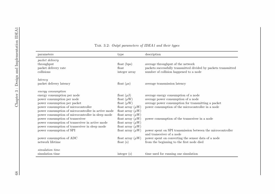
68Chap
ter3:Designan
dIm
plementation
IDEA1
Tab. 3.2: Outpt parameters of IDEA1 and their types
parameters type description
packet deliverythroughput float (bps) average throughput of the networkpacket delivery rate float packets successfully transmitted divided by packets transmittedcollisions integer array number of collision happened to a node
latencypacket delivery latency float (µs) average transmission latency
energy consumptionenergy consumption per node float (µJ) average energy consumption of a nodepower consumption per node float (µW) average power consumption of a nodepower consumption per packet float (µW) average power consumption for transmitting a packetpower consumption of microcontroller float array (µW) power consumption of the microcontroller in a nodepower consumption of microcontroller in active mode float array (µW)power consumption of microcontroller in sleep mode float array (µW)power consumption of transceiver float array (µW) power consumption of the transceiver in a nodepower consumption of transceiver in active mode float array (µW)power consumption of transceiver in sleep mode float array (µW)power consumption of SPI float array (µW) power spent on SPI transmission between the microcontroller
and transceiver of a nodepower consumption of ADC float array (µW) power spent on converting the sensor data of a nodenetwork lifetime float (s) from the beginning to the first node died
simulation timesimulation time integer (s) time used for running one simulation

Chapter 3 : Design and Implementation IDEA1 69
Since the processing units of the existing generic sensor node platforms are mostly
based on 8/16 bits microcontrollers [127], we mainly focus on some power-efficient
microcontrollers. These hardware components can be assembled to construct some COTS
hardware platforms (e.g., MICA2 [27] and MICAz [42]). As stated in section 2.1.2, MICA
motes are commercially available products that have been used widely by researchers
and developers. Microchip PIC16LF88 and MRF24J40 are the main part of the node
developed in our laboratory, named N@L (Node@Lyon), which has been used to establish
an experimental testbed for validating the simulation results of IDEA1. The N@L mote
prototype is depicted in Fig. 3.3.
Fig. 3.3: N@L node prototype
It is powered by 2 AA batteries. The main feature of N@L mote is low power
consumption. It is mainly composed of a PIC16LF88 microcontroller and a MRF24J40
transceiver. Its key feature is power efficient. The current consumption of active operation
mode of PIC16LF88 is only 0.93-1.2mA [18]. Another feature is hardware support of IEEE
802.15.4 standard by MRF24J40.
The microcontroller communicates with the RF transceiver via a SPI bus. For
transmission, the microcontroller needs to write a MAC header and sensor data to the
TXFIFO of RF transceiver. MRF24J40 will automatically add a synchronization header,
PHY header and Frame Check Sequence (FCS), and transmit the packet by using the
IEEE 802.15.4 media access algorithms. After transmission, the RF transceiver will
send the microcontroller an interrupt to report the transmission results. For receiving,

70 Chapter 3 : Design and Implementation IDEA1
MRF24J40 calculates and verifies the cyclic redundancy check (CRC) automatically and
sends an interrupt to the microcontroller to report a receipt of packet. If the packet
requires an acknowledgment (ACK), MRF24J40 will send an ACK automatically. The
microcontroller only needs to handle the sensing operation and read/write packets from/to
the RF transceiver.
In the aspect of communication protocol, IEEE 802.15.4 has been implemented,
including the three MAC algorithms (i.e., non-beacon non -slotted CSMA-CA, beacon-
enabled slotted CSMA-CA and GTS algorithm). Low Rate Wireless Personal Area
Network (LR-WPAN), especially IEEE 802.15.4, is intended to become an enabling
technology for WSN [12][22] which stresses short range operation, low data rate, energy
efficiency, and low cost.
At present, the packet frame format implemented in IDEA1 is mainly focusing on
IEEE 802.15.4. The packet frame format defined in IEEE 802.15.4 standard is presented
in Fig. 3.4.
Fig. 3.4: Packet frame format of IEEE 802.15.4, redrawn from [15]
Preamble sequence is used for synchronizing messages. SFD can indicate the starting
point of packet. A lot of information can be presented by the frame control field, such
as packet type (e.g., data, command, beacon and ACK), security enabled, ACK request,
etc. The frame check sequence is utilized for error detection and correction. The frame
format is implemented as a packet structure in IDEA1. The transmissions between nodes
are at packet-level in order to accelerate the simulation speed. However, the length of
packet can be changed and the transmission time of packets is cycle accurate.

Chapter 3 : Design and Implementation IDEA1 71
In recent years, many radio chips implement the communication protocols
(specifications of PHY and MAC layers) by hardware; for instance, Texas Instrument (TI)
CC2420 supports the IEEE 802.15.4 standard partially by hardware. Users of TI CC2420
must implement the CSMA-CA algorithms by software, such as backoff period waiting
and beacon tracking. However, Microchip MRF24J40 implements the IEEE 802.15.4
completely in hardware. Users only need to load the packet frame to the TXFIFO
buffer of the transceiver and trigger the transmission by sending a command from the
microcontroller to transceiver, and then the transceiver will handle the transmission and
report the transmission result to the microcontroller. A same function can be implemented
by both hardware and software, which refers to the HW/SW partitioning problem. Due to
the advantages of SystemC in HW/SW co-design and co-synthesis, we can model HW/SW
at TLM level and easily handle HW/SW partitioning at lower level.
3.2.4 Graphical User Interface
The GUI is designed as a plug-in to the simulation environment so that the experienced
designers can also write SystemC code directly to configure applications and control
simulations. An example of IDEA1 graphical user interface is presented in Fig. 3.5.
The GUI presented in Fig. 3.5 consists of three major parts: system configuration table
(top-left of the main window) managing all the system parameters that users can set the
input parameters, network topology widget (top-right) showing the relative positions of all
nodes and the radio connections among them, and a console (bottom) displaying the debug
information and simulation log. The users first establish their WSN systems by configuring
the system parameters in the system configuration table such as number of nodes, positions
of nodes and protocol parameters. The connections between two nodes indicated by a solid
line on the topology display window are calculated based on radio propagation models
that condiders many impact factor, such as positions of nodes, transmit power, receive
sensitivity and attenuation factor. Then the simulation can be started by pressing the
’Run’ button (light blue triangle) on the toolbar, which will trigger the execution of final

72 Chapter 3 : Design and Implementation IDEA1
Fig. 3.5: Graphical user interface of IDEA1: A network with 100 nodes is modeled in thisexample
executable simulation program that will read the user setting recorded in an XML file
during runtime. Finally, the simulation results are shown in the console window and the
generated trace file, normally in Value Change Dump (VCD) format, can be viewed by
any waveform-viewing tools.
3.2.5 IDEA1 Features
IDEA1 can quickly model the WSN system at system-level with the detailed parameters
of hardware and software. As a simulator especially for WSN, it also has many other
features that meet the requirements of the special characteristics of WSN. They are as
follows.
• Scalability : The nodes are often deployed in large quantities in many WSN
applications. When simulating these applications, the simulation time should
not augment too much as the number of nodes increases. IDEA1 provides great
scalability as a result of the system-level modeling and its efficient implementation

Chapter 3 : Design and Implementation IDEA1 73
of SystemC code. It has been proved that the simulation speed of IDEA1 is 2 times
faster than NS-2. A detailed analysis will be presented in section 4.3.3.
• Energy aware: IDEA1 can assess accurately the energy consumption of a single
node and the lifetime of network. All the microcontroller and transceiver models in
IDEA1’s library are associated with an energy model based on some experimental
measurements or values from datasheets. The energy models include not only the
current consumptions of all the states, but also the current consumptions and timing
information of the transitions between two states.
• Extensibility : As an extensible simulator, it should be easy to modify the existing
modules or add some new ones. The code of the existing modules in IDEA1 can be
reused to develop new components by the users. In addition, IDEA1 is a component-
based simulation environment, so new hardware or software modules can be easily
integrated to the current library.
• Heterogeneity Support : Many recently deployed WSN applications are heteroge-
neous systems, incorporating a mixture of elements with varying capabilities. In
IDEA1, all the nodes are modeled by SystemC and they can be connected to the
network model as long as they have the compatible interfaces with the network
module.
• Compatibility to the embedded system design flow : Node system design is always an
important topic in the field of WSN. New node systems are modeled normally by
SystemC at first. SystemC has become an emerging de-facto-standard for system-
level modeling. Having a model of the system, it is possible to simulate and verify
it. Once the model is correct, the real hardware can be synthesized starting from its
description. Therefore, IDEA1 provides the node system designers the possibilities
to evaluate the network performance of their new designs at an early stage. And it
also allows the designers to simulate the proposed protocols on new hardware even
if it has not been fabricated. The models developed for the simulation can also be

74 Chapter 3 : Design and Implementation IDEA1
synthesized into lower-level designs.
• Easy to use: SystemC is very easy to learn if the users are familiar with C++
programming, since SystemC is a C++ library. In addition, the users can establish
their system with the components in our library, so they do not have to write any
code. The GUI also provides the users with some other useful functions to facilitate
the control of simulation and the analysis of results.
3.3 Simulation Model Implementations
In this section, we explain the implementations of simulation models of IDEA1 in detail,
including sensor node, microcontroller, transceiver, network and energy models.
3.3.1 Sensor Node Modeling
IDEA1 is a component-based simulator. Each hardware component is modeled as an
individual module of SystemC. A typical model of sensor node is defined, as presented in
Fig. 3.6.
Fig. 3.6: A typical model of sensor nodes
For hardware modeling, sensor is simulated as a stimuli generator that is an interface
specifying how the physical parameters in the environment vary in spatial and temporal

Chapter 3 : Design and Implementation IDEA1 75
terms. The processing unit converts the analog signal from the sensor module into digital
format by a built-in Analog to Digital Converter (ADC), processes the data and sends the
packet to the RF transceiver via a Serial Peripheral Interface (SPI) bus which is a standard
communication type between microcontroller and transceiver. The RF transceiver emits
the packets in the network by different media access protocols. Some connections are
used by the RF transceiver to report interrupts (INT) to the processing unit, such as a
receipt of packet, Clear Channel Assessment (CCA), etc. The processing unit can also
wake up or reset the RF transceiver by two connections relatively. The processing unit
and RF transceiver are modeled as Finite State Machines (FSMs). During simulation,
the state transition traces of each component are recorded. Each state of the hardware
components is associated with a Current Consumption (CC) based on experimental
measurements and their data sheets. The duration and current consumption of each
transition between two states are also identified. Based on this information, the battery
module calculates the energy consumption of each component and its residual capacity
according to particular battery models (e.g., linear model, discharge rate dependent model
and relaxation model [128]) during runtime.
3.3.2 Microcontroller Model
The microcontroller is modeled as a finite state machine, as presented in Fig. 3.7. The
FSM of microcontroller is controlled by the interrupts generated by RF transceivers and
the applications it implements. In the model presented in Fig. 3.7, the application is a
typical one. The microcontroller wakes up periodically by a built-in timer in order to
obtain a sensor data and try to transmit the data to it destination; in addition, it may be
in IDLE state for waiting a RX interrupt from RF transceiver. When the microcontroller
is in the SENSING state, it performs the sensing operating which is modeled by data
generation in the sensor module and analog-to-digital conversion in the microcontroller.
After conversion, it stores the sensor data in a buffer. It will go to either SLEEP or IDLE
state depending on the application specifications if the data size is less than a certain

76 Chapter 3 : Design and Implementation IDEA1
value (the payload field size of the protocol-defined packet); otherwise, it will go to TX
state. In this state, the microcontroller send the sensor data to the RF transceiver via SPI
when the size of sensor data is big enough to construct a packet frame. The transceiver
will send the packet to its destination. The microcontroller quits the TX state until the
transmission of the packet is finished, that is to say it receive a interrupt report of the
transmission results from RF transceiver. After a transmission, the microcontroller may
stay in TX state and transmit another packet, or it will go to SLEEP or IDLE state.
When the microcontroller is in IDLE state, if a packet is received by RX transceiver, it
will go to RX state for reading the packet via SPI by an interrupt from RF transceiver.
If the packet is intended to other nodes, the microcontroller need to resend it to RF
transceiver in order to forward it to its destination; otherwise, the microcontroller will go
to SLEEP or IDLE state.
Fig. 3.7: A typical model of microcontroller
The microcontroller model presented in Fig. 3.7 is a typical one. Any specific
microcontroller model can be developed based on this typical model. For specific
microcontrollers, the current consumptions of each states and some timing parameters
may need to be update; moreover, according to different RF transceivers, the RX and TX
process may be different. It depends on the hardware implementations of communication
protocols by the RF transceivers.

Chapter 3 : Design and Implementation IDEA1 77
When the microcontroller is in TX state, the node (both microcontroller and RF
transceiver) need to perform specific communication protocols in order to access the
channel and avoid collisions of packet. The protocols can be implemented either by RF
transceiver with hardware support or by microcontroller with software. In the latter case,
the TX state of microcontroller will be divided into many sub-states. For example, if the
IEEE 802.15.4 MAC protocols presented in section 2.3.2.3, the TX state will be replaced
by the following sub-states, as presented in Fig. 3.8.
Fig. 3.8: State machine for microcontroller of IEEE 802.15.4 MAC protocol
In Fig. 3.8, it is an example of IEEE 802.15.4 slotted CSMA-CA algorithm. When
entering to TX state, the microcontroller first backoff a random duration and check the
channel. If the channel is free, it will start transmitting a packet. The backoff period
boundaries should be aligned with the superframe slot boundaries and the microcontroller
should ensure that the transceiver commences all of its transmissions on the boundary
of a backoff period. One backoff period includes 20 symbols, corresponding to 320 µs if

78 Chapter 3 : Design and Implementation IDEA1
the data rate is 250kbps. For the unslotted CSMA-CA algorithm, there is no need to
locate the backoff boundary and the clear channel assessment only need to be performed
once. For the GTS algorithm, the algorithm is very simple, after the receipt of a beacon
packet, the microcontroller wait until its slot to transmit without any backoff or CCA
mechanisms.
The sensing operation has the first priority that can interrupt any task. If the
sensing timer expires when a microcontroller is in other states except SENSING state,
it will suspend ongoing task, start converting sensor data, and resume its old task after
the sensing. If an interrupt from RF transceiver occurs when the microcontroller is in
SENSING state, the interrupt will be recorded and handled after the sensing operation.
In order to save energy, nodes should go to SLEEP mode as long as they have no data
to send. However, the transition from SLEEP mode to ACTIVE mode of microcontroller
takes some time, for example, PIC16LF88 spends 4 ms to wake up from sleep to INTOSC
mode [18]. Sometimes, the interval between two consecutive sensing operations is less the
transition time of microcontroller. We proposed an algorithm to handle the concurrency
between the sensing and other operations, as presented in Fig. 3.9.
When the sensing timer expires, this algorithm will be invoked. If the sensing interval
is less than or equal to the transition time, the nodes do not go to SLEEP mode and they
set the sensing timer as the sensing interval; otherwise, they go to SLEEP mode after
sensing if they do no need to send the data immediately and they set the sensing timer
as a value that is the sensing interval minus the transition so that they have enough time
to wake up before sensing. Nodes firstly set the timer for the next sensing operation.
Secondly, they read the sensor data and wait a sensing operation duration. After sensing,
the nodes store the sensor data in a buffer. If the previous state is not SLEEP, they will
go to the previous state; otherwise, they will transmit a packet when the size of sensor
data is bigger than the the payload field size of protocol-defined packet.
The transition from one state to another is controlled by the system configuration
and network simulation. The microcontroller has to go to SENSING state whenever

Chapter 3 : Design and Implementation IDEA1 79
Fig. 3.9: Algorithm for handling the concurrency of sensing and other operations
the sensing timer expires, where the sample interval is an input parameter of system
configuration. In addition; it will go to RX state when it receive an interrupt form
RF transceiver, which is a result of network simulation. However, the time staying in
SENSING and RX states is constant. They are determined by the software executions.
In the SENSING state, the microcontroller performs the analog to digital conversion. In
the RX state, it reading the RXFIFO of RF transceiver via SPI reading. The time of this
operation depends on the SPI communications speed, the time of software configuration

80 Chapter 3 : Design and Implementation IDEA1
of SPI hardware and the length of the packet. The time staying in TX state is determined
by SPI writing and the packet transmission.
The embedded software running on microcontroller is divided into different tasks,
such as analog to digital conversion and SPI communication. Before the simulations,
the execution time of these tasks need to be inputted by users. The time for an analog
to digital conversion or SPI communication is composed by two parts. One is the time
to configure the ADC or SPI hardware by software, and the other is the conversion or
communication duration of hardware.
The software execution time of each tasks can be obtained by their C or assembly
codes. For some new architectures that are still under development, many execution time
estimation methods for embedded systems can be applied in our model like the SystemC-
based hybrid approach proposed in [129]. This approach combines the advantages
of simulation-based and analytical approaches. In the first step, cycle-accurate static
execution time analysis is applied at each basic block of a cross-compiled binary program
using static processor models. After that, the determined timing information is back-
annotated into SystemC for a fast simulation of all effects that can not be resolved
statically.
At present, in the library of IDEA1, there are two microcontroller models, ATMEL
ATMega128 and Microchip PIC16LF88. Some specifications of these two models will be
introduced in the following two subsections.
3.3.2.1 Model of ATMEL ATMega128
In this section, the timing specifications of ADC and SPI tasks of ATMEL ATMega128
are introduced. The energy consumptions of each operation state will be presented in the
energy model part, section 3.3.5.
According to the data sheet of ATMega128 [16], the ADC clock frequency should be
fixed between 50 kHz and 200 kHz to get a maximum resolution; therefore, if the CPU

Chapter 3 : Design and Implementation IDEA1 81
operation frequency is 7.3728MHz, the division factor of ADC prescaler should be set to
64 or 128 in order to get a 115.2 or 57.6 kHz ADC clock frequency; thus the conversion
time to this two division factor is 217µs and 434µs. The smaller one is chosen as the value
of this parameter in our simulations. The time taken by the microcontroller to configure
and control the ADC hardware can be estimated by the assembly code of this task. It
takes 12 clock cycles for the software ADC configuration; one analog to digital conversion
is therefore 218.6µs.
If the SPI prescaler is set to 2 and the operating frequency of microcontroller is 7.3728
MHz, ATMega128 needs to spend 2.17 µs to transmit one byte by SPI hardware. The
configuration software execution time is calculated based on the C and assembly codes.
The C code of SPI communication is presented in Listing. 3.1.
Listing 3.1: C code example for SPI communication of ATMega128
FASTSPI STROBE( int a )
PORTB &= ˜BM(CSN) ; //2 c l o c k c y c l e
SPDR = a ; //1 c l o c k c y c l e
while ( ! ( SPSR & BM(SPIF) ) ) ; // wai t ing f o r the end o f SPI communication .
PORTB |= BM(CSN) ; //2 c l o c k c y c l e
FASTSPI WRITE FIFO(p , c )
SPI ENABLE( ) ; //2 c l o c k c y c l e
SPDR = CC2420 TXFIFO ; //1 c l o c k c y c l e
while ( ! ( SPSR & BM(SPIF) ) ) ; // wai t ing f o r the end o f SPI communication .
for (UINT8 spiCnt = 0 ; spiCnt < ( c ) ; spiCnt++) // f o r loop , 18 c l o c k
c y c l e
SPDR = ((BYTE∗) (p ) ) [ spiCnt ] ; //1 c l o c k c y c l e
while ( ! ( SPSR & BM(SPIF) ) ) ; // wai t ing f o r the end o f SPI communication .
SPI DISABLE( ) ; //2 c l o c k c y c l e

82 Chapter 3 : Design and Implementation IDEA1
BOOL basicRfSendPacket (BASIC RF TX INFO ∗pRTI)
// Write the packet to the TX FIFO
FASTSPI WRITE FIFO( (BYTE∗) &packet , frameLength ) ;
FASTSPI STROBE(CC2420 STXON) ; // enab l e the t ransmis s ion .
In this example, the RF transceiver is TI CC2420. It takes ATMega128 (0.68 + 2.17)
µs to transmit one strobe command and ((0.68 + 2.17) + (2.577 + 2.17) ∗ lengthFrame)
µs to transmit a data frame with a length of lengthFrame bytes. Unlike MRF24J40, it
does not need to write the address of each byte when writing a frame of several bytes to
CC2420. It only need to tell CC2420 that the frame is intended to TXFIFO and then
send the frame continually. To transmit one packet, the microcontroller needs to send
the data frame and a TX command to the transceiver. Therefore, ATMega128 needs
(2 ∗ (0.68 + 2.17) + (2.577 + 2.17) ∗ lengthFrame) µs to transmit a packet of lengthFrame
bytes to RF transceiver.
3.3.2.2 Model of Microchip PIC16LF88
In this section, the timing specifications of ADC and SPI tasks of Microchip PIC16LF88
are introduced.
An analog to digital conversion of PIC16LF88 takes 65.974µs, including 54µs
computation time (108 instruction cycles with 8MHz clock frequency) and 11.974µs
acquisition time (Minimum Required Acquisition Time [18]). One instruction includes
4 oscillator cycles in PIC16LF88. The computation time includes the configuration of
ADC hardware and read of ADC result. The C code used in this evaluation is presented
in Listing. 3.2.
Listing 3.2: C code example for analog to digital conversion of PIC16LF88
unsigned int ReadADC( )

Chapter 3 : Design and Implementation IDEA1 83
/∗ I n i t i a l i s i n g the ADC channel 0 ∗/
TRISA0 = 0 ; //3 c y c l e s
/∗ Analogue−RA0/RA1/RA3 D ig i t a l−RA2/RA5 ∗/
ADCON1 = 0b10000100 ; //3 c y c l e s
/∗ S e l e c t i n g ADC channel ∗/
ADCON0 = 0b00000001 ; // Enable ADC, 3 c y c l e s
ADIE = 0 ; // Masking the in t e r rup t , 3 c y c l e s
ADIF = 0 ; // Rese t t in g the ADC in t e ru p t b i t , 3 c y c l e s
ADGO = 1 ; // S tar ing the ADC process , 1 c y c l e s
while ( !ADIF) continue ; // Wait f o r convers ion complete
volati le unsigned int ADC VALUE;
ADC VALUE = ADRESL; // Get t ing LSB of CCP1, 9 c y c l e s
ADC VALUE += (ADRESH << 8) ; // Get t ing HSB of CCP1 , 60 c y c l e s
return (ADC VALUE) ; // Return the va lu e o f the ADC process , 9 c y c l e s
The number of instruction cycle needed for each statement is also provided in
Listing. 3.2. Before the start of conversion, the initialization of ADC channel and interrupt
is performed. After conversion, the results is stored in a variable and returned. Note that,
the while loop is waiting for the hardware conversion to be finished, which is not included
in the computation time.
For the SPI communication of PIC16LF88, if the SPI prescaler is set to 4 and
the operating frequency of microcontroller is 8 MHz, PIC16LF88 needs to spend 4 µs
to transmit one byte by SPI hardware. The configuration software execution time is
calculated based on the C and assembly codes. The C code of SPI communication is
presented in Listing. 3.3.
Listing 3.3: C code example for SPI communication of PIC16LF88
void s p iw r i t e s h o r t ( in t8 address , i n t8 va lue )
output low (CS) ; //1 cyc l e
s p i w r i t e ( ( ( address<<1) & 0b01111111 ) | 0x01 ) ; //8 c y c l e s + SPI
t ransmis s ion time
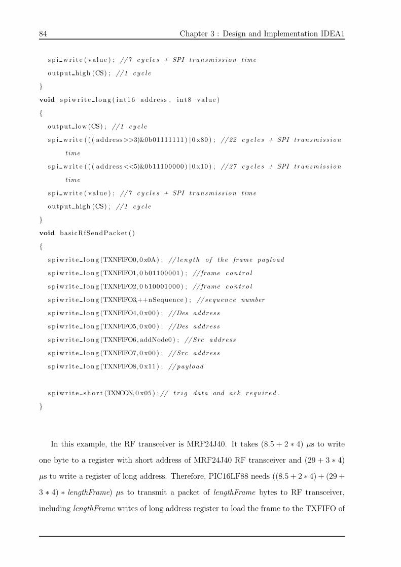
84 Chapter 3 : Design and Implementation IDEA1
s p i w r i t e ( va lue ) ; //7 c y c l e s + SPI t ransmis s ion time
output high (CS) ; //1 cyc l e
void s p iw r i t e l o ng ( in t16 address , i n t8 va lue )
output low (CS) ; //1 cyc l e
s p i w r i t e ( ( ( address>>3)&0b01111111 ) |0 x80 ) ; //22 c y c l e s + SPI t ransmis s ion
time
s p i w r i t e ( ( ( address<<5)&0b11100000 ) |0 x10 ) ; //27 c y c l e s + SPI t ransmis s ion
time
s p i w r i t e ( va lue ) ; //7 c y c l e s + SPI t ransmis s ion time
output high (CS) ; //1 cyc l e
void bas icRfSendPacket ( )
s p iw r i t e l o n g (TXNFIFO0, 0 x0A) ; // l en g t h o f the frame payload
s p iw r i t e l o n g (TXNFIFO1, 0 b01100001 ) ; // frame con t r o l
s p iw r i t e l o n g (TXNFIFO2, 0 b10001000 ) ; // frame con t r o l
s p iw r i t e l o n g (TXNFIFO3,++nSequence ) ; // sequence number
s p iw r i t e l o n g (TXNFIFO4, 0 x00 ) ; //Des address
s p iw r i t e l o n g (TXNFIFO5, 0 x00 ) ; //Des address
s p iw r i t e l o n g (TXNFIFO6, addNode0 ) ; //Src address
s p iw r i t e l o n g (TXNFIFO7, 0 x00 ) ; //Src address
s p iw r i t e l o n g (TXNFIFO8, 0 x11 ) ; // payload
s p iw r i t e s h o r t (TXNCON,0 x05 ) ; // t r i g data and ack requ i r ed .
In this example, the RF transceiver is MRF24J40. It takes (8.5 + 2 ∗ 4) µs to write
one byte to a register with short address of MRF24J40 RF transceiver and (29 + 3 ∗ 4)
µs to write a register of long address. Therefore, PIC16LF88 needs ((8.5 + 2 ∗ 4) + (29 +
3 ∗ 4) ∗ lengthFrame) µs to transmit a packet of lengthFrame bytes to RF transceiver,
including lengthFrame writes of long address register to load the frame to the TXFIFO of

Chapter 3 : Design and Implementation IDEA1 85
RF transceiver and one write of short address register (Transmit Normal FIFO Control
Register of MRF24J40) to enable the transmission.
3.3.3 Transceiver Model
The state transition of RF transceiver is triggered by three types of events, including
protocol implemented, microcontroller commands and network events. Different
transceivers may have various protocols implemented. However, for microcontroller
commands and network event, we have summarized some common events. Based on
this, a universal model of transceivers is developed, as illustrated in Fig. 3.10.
Fig. 3.10: A typical model of transceiver
The transceiver is woken up by a command of micrcontroller and wait for a specified
crystal oscillator start-up time to enter IDLE state. The transitions from IDLE state to
RX FRAME or TX FRAME states are also triggered by commands of microcontroller.
When a packet is received in RX FRAME state, the transceiver may automatically go to
TX FRAME state to send back an acknowledgment if an ACK is required by the received
packet.
For specific transceivers, some parameters need to be fixed, including the data

86 Chapter 3 : Design and Implementation IDEA1
rate, data frame needed to transmit from microcontroller to transceiver and the SPI
communication speed.
3.3.3.1 Transceiver Model of TI CC2420 and CC1000
TI CC2420 supports the IEEE 802.15.4 PHY layer with a 250 kbps data rate in the 2.4
GHz frequency band, but the maximum data rate of TI CC1000 is 76.8 kbps. TI CC2420
can add a preamble Sequence, start of frame delimiter and frame check sequence to the
data frame automatically; however, for TI CC1000, the microcontroller needs to write
these fields of packet to transceiver by SPI communication.
Because TI CC2420 and CC1000 do not implement any channel access algorithms with
hardware, the models of these two transceivers are almost the same with that presented
in Fig. 3.10. Two small changes have to be applied for CC1000. One is that CC1000
do not have IDLE state. It is woken up by the microcontroller and go directly to RX or
TX states. The other is that CC1000 do not support automatic address check and ACK
transmission.
3.3.3.2 Transceiver Model of Microchip MRF24J40
Since Microchip MRF24J40 provides hardware support of IEEE 802.15.4 MAC protocols,
its models of finite state machine extend the typical model by adding some protocol based
states and transitions of states. The three IEEE 802.15.4 media access algorithms has
been modeled, including unslotted CSMA-CA, slotted CSMA-CA and guaranteed time
slots (GTS). Therefore, three finite state machines of transceiver are developed according
to these MAC algorithms.
According to the tasks of unslotted CSMA-CA algorithm, the RF transceiver has 7
states, as presented in Fig. 3.11.
The transceiver is set to sleep mode or woken up from sleep modes by commands of
microcontroller. Like TI CC1000, there is no IDLE state in MRF24J40; therefore, the

Chapter 3 : Design and Implementation IDEA1 87
Fig. 3.11: Model of MRF24J40 in non-beacon mode with CSMA-CA algorithm
transceiver is woken up directly to RX mode. When a packet is received in RX mode, the
transceiver will inform the micrcontroller by an interrupt and automatically send back an
ACK packet immediately if an ACK is required. If a transmission of packet is triggered
by the microcontroller, the transceiver will use the unslotted CSMA-CA algorithm to
transmit the packet. After the transmission of a packet, the RF transceiver waits a fixed
duration for the transmission being acknowledged if the ACK request bit in the frame
control field of the packet is set. The transmission is successful if the ACK is received in
time. The transceiver will report the transmission results to the microcontroller and go to
RX state. A transmission may fail after macMaxCSMABackoff times attempts of clear
channel assessment or macMaxFrameRetries times failures of receiving an ACK packet.
A failure of receiving an ACK packet may be caused by the collisions of either data packet
or ACK packet. The microcontroller can set the RF transceiver to SLEEP mode from
any state immediately by a command.
The process of slotted CMA-CA algorithm is similar to the unslotted algorithm except
the backoff period boundaries of every node should be aligned with the superframe slot
boundaries and the MAC sublayer should ensure that the PHY commences all of its
transmissions on the boundary of a backoff period. The model of MRF24J40 with slotted

88 Chapter 3 : Design and Implementation IDEA1
CSMA-CA algorithm is presented in the Fig. 3.12.
Fig. 3.12: Model of MRF24J40 in beacon mode with slotted CSMA-CA algorithm
If it is a coordinator, the BEACON ACQUIREMENT/TRANSMISSION state is to
broadcast a beacon packet; for a device node, it is BEACON ACQUIREMENT. In order
to send a packet, the transceiver should first receive a beacon packet to be synchronized
with the coordinator. On a successful receipt of beacon packet, the node may go to
RX state if it has no data to send, or it will start a new transmission by using slotted
CSMA-CA algorithm. Before and after the random backoff, the transceiver should ensure
that the remaining CSMA-CA operations can be undertaken before the end of the CAP.
If the remaining number of backoff periods in the CAP is not enough for the random
backoff, the transceiver will continue the backoff countdown and resume it at the start
of the CAP in the next superframe. After the random backoff, if the remaining time is
not enough for the transaction, including two CCAs, one transmission of data packet and
one transmission of ACK packet, the transceiver will wait until the next superframe and
perform a new random backoff delay again. Therefore, on receipt of a beacon packet, the

Chapter 3 : Design and Implementation IDEA1 89
transceiver may go the backoff state to resume a transmission of the previous superframe.
To ask a GTS usage, the node must send a GTS request command to the coordinator
during CAP by using the slotted CSMA-CA algorithm. On receipt of this command, the
coordinator sends an ACK. Then, the node keeps tracking the beacon frames for at most
4 superframes to verify which time slot is allocated. The information is located in the
GTS descriptor field of the beacon packet. A minimum length of CAP with 440 symbols
must be guaranteed in every superframe. After the GTS request is acknowledged by the
coordinator, the node keeps tracking the beacon packet and sends data during its GTS
slot, as presented in Fig. 3.13.
Fig. 3.13: Model of MRF24J40 in beacon mode with GTS algorithm
On a successful receipt of beacon packet, the transceiver may go back to SLEEP state
if it has no data to send or it will wait until its GTS slot to transmit a packet. For the
transmission of GTS algorithm, ACK is not required, because the channel is allocated
exclusively to one node.
3.3.4 Network Modeling
The network model connects each node, manages the network topology and implemented
the radio propagation. In this section, two questions will be answered.
• Packet Transmission: how a packet from one node can be transmitted to another
node?
• Radio propagation model : what happens during the transmission?

90 Chapter 3 : Design and Implementation IDEA1
3.3.4.1 Packet Transmission
In this section, the packet transmission process in IDEA1 is described. As stated
in section 3.1.1, SystemC simulation executes in three distinct major phases, includes
elaboration, simulation and postprocessing. During the elaboration phase, a network and
several node objects are instantiated. Each nodeProxy object registers its information to
the network object. The registered information includes its address, position, TX power
and RX sensitivity. The network model establishes a two-dimension topology array based
on this information and the radio propagation models. A detailed description of the
implemented radio propagation models will be provided in section 3.3.4.2. As detailed
in [4], the network object also contains a pointer array that points to each nodeProxy
instance, which is used to send a packet to the relative nodes.
When the simulation runs, if a node, named as node A, wants to send a packet to a
node B, it firstly calls a public function of the network class to calculate the transmission
time of this packet. After waiting the transmission duration, the nodeProxy sends the
packet to the network model. On receipt of this packet, the network model will send that
packet immediately to all the nodes that are in the transmission range of the transmitter.
By doing these, the transmission duration is modeled.
The network model also assign a counter to each node which is used to check the
transmission validity with respect to collisions. The counter holds the numbers of active
transmissions that can reach a relative nodes at a given time. If it is bigger than one, a
collision occurs. When a node receives a packet, it check the destination address of that
packet and accept it if the addresses match.
3.3.4.2 Radio Propagation Model
Radio propagation model is used to predict the received signal power of each packet. Every
transceiver has a receiving sensitivity which is a threshold. If the power of a signal arrived
at a transceiver is below the receiving sensitivity of this transceiver, it will not be able to

Chapter 3 : Design and Implementation IDEA1 91
be successfully decoded. At present, two models have been implemented in IDEA1: the
free space propagation model [130] and the ITU (International Telecommunication Union)
indoor propagation model [131]. They present two typical working environments of WSN
applications, i.e., indoor and outdoor scenarios. The users can choose a propagation model
at the beginning of simulation by setting a system parameters. If these two models are
not accurate enough for the specific applications of some users, they can add some more
special radio propagation models in IDEA1.
The free space propagation model has the following form:
Pr(d) =PtGtGrγ
2
(4π)2d2(3.1)
Where Pr(d) presents the received power of a signal at the part of receiver which is
located d meters away from the transmitter. Pt is the TX power of a signal at the part
of transmitter. Gt and Gr are the antenna gains of the transmitter and the receiver
respectively. γ is the wavelength.
The ITU indoor propagation model is formally expressed as:
Ltotal = 20× log10f +N × log10d+ Lf(n)− 28 (3.2)
Where Ltotal is the total path loss. f is the transmission frequency and its unit is MHz. N
is the distance power loss coefficient. Lf is the floor penetration loss factor and its unit
is dB. Both the distance power loss coefficient and the floor penetration loss factor have
been given some recommended values by IUT based on various measurement results which
can be found in [131]. n is the number of floors between the transmitter and receiver.
3.3.5 Energy Model
Many energy models have been developed and implemented in the existing simulation
tools for WSN. For example, a power model of different hardware components have

92 Chapter 3 : Design and Implementation IDEA1
been included in SensorSim [97]. In this model, the power consumption of each
hardware component is considered, but the CPU and sensor device models have not been
implemented. A measured prototype power consumption model for Tampere University of
Technology Wireless Sensor Network (TUTWSN) motes is provided in [132]. The power
consumptions of TUTWSN mote in different operation modes (e.g., sleep, RX and TX)
have been measured; however, the transition between two states has not been considered.
An improved energy model [133] has been implemented in OMNeT++. In this model,
both the the transition energy cost for switching between the radio operational states
and the energy consumption of microcontroller have been considered. However, in the
implementation of this model, the authors assume that the microcontroller follows the
same sleeping schedule of the radio interface; nevertheless, the processor can be in sleep
mode when the RF transceiver is listening to the channel and woken up by the latter when
a packet is received. IDEA1 overcomes these limitations by component-based hardware
models of sensor nodes which allow each components to operate independently.
In IDEA1, each state of the main hardware components in a sensor node is associated
with a current load. The duration and current consumption of each transition between
two states are also identified. During the simulation, the states of these components are
updated according to software execution and network events. The energy consumed by
node i can be calculated as follows.
Ei =
N∑
j=0
(
M∑
k=0
Eijk +
O∑
l=0
Eijl)
=
N∑
j=0
(
M∑
k=0
V · Iijk · tijk +
O∑
l=0
V · Iijl · tijl)
(3.3)
Where Eijk presents the energy consumption of the kth state of the jth component of node
i, and Eijl presents the energy consumption of the lth state transition of the jth component
of node i. The node has N components consuming energy. Each component has M states
and O transitions. During the simulation, the state transition traces of each component
are recorded; thus the time spent on different states and transitions, tijk and tijl, is known.

Chapter 3 : Design and Implementation IDEA1 93
Based on this information, the battery module calculates the energy consumptions of each
component as well as the network lifetime during runtime.
The current consumptions of different operation modes need to be calibrated by
real measurements. A testbed has been established to calibrate the energy model and
validate the simulation results. It will be described in section 4.2. In this chapter, the
current consumptions of the main operation modes of the hardware components of MICAz
and N@L motes are summarized according to the data sheets of their main hardware
components [16][17][18][19], as presented in Table 3.3 and Table 3.4.
Tab. 3.3: Current consumptions of MICAz mote [16][17]
Microcontroller (ATMEL ATMega128) Transceiver (TI CC2420)mode current consumption mode current consumption
(transition time) (transition time)PowerDown 0.3µA PowerDown 17µAPowerSaving 8.9µA IDLE 426µAIDLE 4mA RX 18.8mAActive 9mA TX(0dBm) 17.4mAPowerSaving->Active n/a TX(-5dBm) 13.9mA
TX(-10dBm) 11.2mATX(-25dBm) 8.5mAPowerDown -> IDLE 426µA(1ms)IDLE -> RX 18.8mA(192µs)IDLE -> TX 6.7mA(192µs)
Tab. 3.4: Current consumptions of N@L mote [18][19]
Microcontroller (Microchip PIC16LF88) Transceiver (Microchip MRF24J40)mode current consumption mode current consumption
(transition time) (transition time)Sleep 0.01∼8µA Sleep 2µAActive 0.93∼1.2mA RX 19mASleep->Active n/a(4mA) TX 23mA
SLEEP -> RX or TX n/a(2ms)TX -> RX n/a(192µs)RX -> TX n/a(192µs)
In Table 3.3, the timing information and current consumptions of transitions from
power saving states to Active state of the microcontroller have not been found in its data
sheet. The minimum current consumption of MICAz motes is 17 µA when the whole
system is in sleep mode. The current consumption increases to 4 or 9 mA when the

94 Chapter 3 : Design and Implementation IDEA1
microcontroller is woken up. It takes the transceiver 1 ms to wake up from power down
state to IDLE state to wait for the crystal oscillator to be stable. When this mote is
transmitting packets, its current consumption is 26.4 mA corresponding to 0 dBm TX
power. The transceiver also needs 192 µA to transit from IDLE to RX or TX states.
In Table 3.4, the current consumptions of the state transitions of N@L mote are not
found in the data sheets of its microcontroller and transceiver. Both PIC16LF88 and
MRF24J40 do not support an IDLE state. PIC16LF88 is an low power microcontroller.
Its active current consumption is only 0.93∼1.2 mA.
3.4 Simulation Output
There are three kinds of simulation output in IDEA1, including simulation log, event
sequence tracing file and sensor data received by nodes.
3.4.1 Simulation Log
The simulation log is used to debug the model implementations and show the network
behaviors. The designers can output debug information when an event occurs to verify
whether this event is triggered with correct logic. An example is presented in Fig. 3.14.
In this example, we can observe a complete transmission process of the transceiver of
node0. After one failed channel access, node1 delay a random number of backoff duration,
and then successfully find a free channel. On reception of the packet from Node0, the
coordinator sends an acknowledgment back. After receiving the ACK packet, Node0
go to SLEEP mode since it has no data to transmit. When the coordinator is sending
acknowledgment packet to Node0, the transceiver of node3 finds the channel is busy at
8448 µs by CCA.
Many statistical results of network behaviors are attached at the end of simulation
log, including aspects of throughput, packet delivery latency, power consumptions and

Chapter 3 : Design and Implementation IDEA1 95
Fig. 3.14: An example of simulation log
simulation time.
3.4.2 Event Sequence Tracing
During the simulation is running, the states of every hardware components and the
variables are updated continually. SystemC provides users a sc trace module to track
signals and records the values of signals into a file in Value Change Dump (VCD) format,
which can be displayed graphically by using waveform-viewing tools. The event sequence
tracing is analyzed to verify and refine the model implementations. Fig. 3.15 presents an
example of event sequence tracing.
A typical carrier sensing multiple access process is presented in this example. The
states of microcontroller and transceiver are presented as numbers. The meaning of each
state is also illustrated in Fig. 3.15. Node1 finds the channel being busy when node0 is
emitting data to the channel; therefore it waits for a random number of backoff periods

96 Chapter 3 : Design and Implementation IDEA1
Fig. 3.15: An example of event sequence tracing
to retransmit the packet.
The packet transmission process among different hardware components and network
is also presented. The packet with a value of 205 in Fig. 3.15 is transmitted from node0
to the network module and to the transceiver and microcontroller of the coordinator, as
shown by the arrows.
Depending on the event sequence tracing, we can also verify the timing accuracy at
cycle accurate level. For the slotted CSMA-CA algorithm, all the transmissions should
be aligned with the backoff boundary. As indicated by two vertical lines in Fig. 3.15,
the transmissions of node0 and node1 have started exactly at the beginning of a backoff
boundary.
The event sequence trace method can provide more comprehensive informations than
simulation log. Every state transition of interested variables is recorded in the VCD file;
on the contrary, the simulation log only tracks the event where a print function is invoked.
However, the simulation log is more flexible and readable; for example, the transmission
results (e.g., failure or success) can be attached in the simulation log directly.

Chapter 3 : Design and Implementation IDEA1 97
3.4.3 Sensor Data
At present, sensors are modeled as an individual module in IDEA1. The sensor module
generates sensor data in two ways. One is random generation, and the other is read
the real measured data in a data file. Some specific sensor chips will be modeled later.
Fig. 3.16 presents an example of the measured sensor data.
Fig. 3.16: Measured sensor data by N@L mote
The data is measured by one sensor of N@L mote, PZT PIC255 piezoelectric sensor,
and a sensor amplifier circuit based on TLV2772 from Texas Instrument. During IDEA1
simulation, every node reads its data from its sensor data file and transmits the data to the
coordinator by using some communication algorithms. After receiving the packets from
nodes, the coordinator stores the sensor data to different files according to every node.
These files can be compared with the original sensor data files to analyze the packet lost.

98 Chapter 3 : Design and Implementation IDEA1
3.5 Conclusion
In this chapter, a novel system-level WSN simulator, named IDEA1, is presented. It is
developed in SystemC and C++, which makes the simulation to be a part of the embedded
system design. It enables the design space exploration at an early stage and supports a
modular design pattern of sensor nodes and WSN applications. Many COTS hardware
platforms have been modeled and the IEEE 802.15.4 standard has been implemented. An
energy model has been implemented on all the hardware component models of IDEA1.
In next chapter, the performance of IDEA1 will be evaluated. The accuracy of the
simulation results of IDEA1 will be validated by some real measurements of a testbed. The
simulation results of IDEA1 will also be compared with NS-2, a widely-used simulator in
WSN field. Other performances of IDEA1, like simulation speed and power consumption
analysis, will also be evaluated.
Chapter 4 : Performance Evaluation of IDEA1 99
Chapter 4 :
Performance Evaluation of IDEA1

100 Chapter 4 : Performance Evaluation of IDEA1

Chapter 4 : Performance Evaluation of IDEA1 101
In this chapter, the performance of IDEA1 is evaluated, especially in two aspects:
accuracy and simulation time. For the accuracy validation, the simulation results of
IDEA1 are compared with some measurements on a testbed composed of 9 nodes. The
simulation of IDEA1 is also compared with NS-2, the most widely-used simulator in the
research of WSN, including the comparisons of simulation results and simulation time.
This chapter is organized as follows. Section 4.1 introduces the metrics used to evaluate
the network performances. Section 4.2 describes the testbed establishment and shows
the comparisons between the testbed measurements and simulation results. Section 4.3
presents the simulation results of both IDEA1 and NS-2 to an IEEE 802.15.4 sensor
networks. The differences between these two simulators are summarized. Finally, section
4.4 concludes this chapter.
4.1 Performance Metrics
Four metrics are used to evaluate the network performances in the testbed experiments
and comparisons with NS-2. They are defined as follows.
• Packet Delivery Rate (PDR): PDR is used to evaluate the network throughput. It
is the ratio of the number of packets successfully received to the number of packets
generated by nodes.
• Average Latency (AL): Latency of a packet is the duration from the generation of
the last sensor data in the packet to the receipt of this packet by coordinator. AL
is an average latency of all packets that successfully received by coordinator. If the
packets only contain one sensor data, AL is also the average latency of sensor data;
however, if several sensor data are transmit in one packet, the latency of a sensor
data is AL plus the interval between this data to the last sensor data.
• Energy Consumption per Packet (ECPkt): ECPkt is the average energy consumed
for successfully transmitting one packet.

102 Chapter 4 : Performance Evaluation of IDEA1
• Average Power Consumption (APC): APC is used to measure the average power
consumption per node which is a basic parameter to predict the lifetime of a sensor
node and the network.
4.2 Experimental Validation
To validate the accuracy of IDEA1 simulation, a testbed of 9 nodes is built. Two kinds
of measurements have been done. One is the measurements of the current consumptions
of every operation modes of an individual sensor node in order to calibrate the energy
model, which will be used in the simulation of IDEA1. The other one is the measurements
on the network testbed of 9 nodes.
4.2.1 Calibration of the Energy Model
Initially, the energy model needs to be calibrated by some experimental measurements.
The current consumptions of every operation mode of hardware components are measured.
Our measurement setup is illustrated in Fig. 4.1.
Fig. 4.1: Hardware measurement configuration
One resistor of 1 Ω was placed series with the power supply of a node (named as node0)

Chapter 4 : Performance Evaluation of IDEA1 103
Tab. 4.1: Measured current consumptions of N@L motes (3.3 V VDD and 8 MHZ clockfrequency)
PIC16LF88 microcontroller MRF24J40 RF transceiveractive 1.386mA sleep 17µAsleep 7µA RX 23.504mAsleep->active 7µA/1.846ms TX(0dBm) 23.961mA
TX(-10dBm) 22.901mATX(-20dBm) 22.631mATX(-30dBm) 22.409mAsleep-> RX 6.7mA/720µssleep->TX 6.7mA/720µs
in order to measure the current consumption of the node by the voltage across this resistor.
The output of the voltage generator is adjusted to ensure that the node has a 3.3V power
supply. An instrumentation amplifier [134] with a gain of 76 is used to amplify the voltage
across the resistor. Tektronix MSO2012 mixed signal oscilloscope [135] is used to track
the output of this amplifier with the highest possible resolution. Tektronix MSO2012
provides a 1 GS/s sample rate. By doing this, the energy consumption of node0 can be
measured.
A set of micro-benchmarks have been developed to isolate the hardware consumption
of microcontroller and transceiver in order to obtain the current consumptions of each
operation mode. For the low current consumption of sleep mode, we use a digital multi-
meter that can capture extremely small current. The current consumptions of N@L motes
is listed in Table 4.1.
As shown in Table 4.1, both the microcontroller and transceiver need a period of time
to wake up from the sleep mode. The current consumptions of the transitions between
two states that are not available in data sheet are also measured.
4.2.2 A Testbed of Sensor Network
4.2.2.1 Testbed Establishment
A star topology testbed of 9 N@L motes is built, as illustrated in Fig. 4.2.

104 Chapter 4 : Performance Evaluation of IDEA1
Fig. 4.2: Testbed Measurement Configuration
This network consists of eight nodes and one coordinator. The nodes read a senor
data (an integer of one byte generated randomly) periodically. The reading frequency is
presented as sample rate. A sample rate is 10, which means that the node read the sensor
data every 0.1 s. The nodes send the sensor data to the coordinator immediately after the
data is read by using the IEEE 802.15.4 unslotted CSMA-CA algorithm. If the sensing
timer expires when the nodes is transmitting a old sensor data, the microcontroller will
store the new sensor data in a one-byte buffer. However, if the sensing tiler expires when
there is already a sensor data in the buffer waiting to be sent, the new sensor data will
replace the old sensor data in the buffer to enable a short latency of sensor data.
The parameters of the unslotted CSMA-CA algorithm (e.g., macMinBE, macMaxC-
SMABackoffs, macMaxFrameRetries, etc.) are set as the default values defined in IEEE
802.15.4 standard [15]. The TX power of RF transceiver is set to 0 dBm. The nodes
go to SLEEP mode after the transmission is finished. The transmission is successful if
an acknowledgment (ACK) is received; otherwise, it fails after macMaxCSMABackoffs
attempts of channel access failure or macMaxFrameRetries attempts of retrying to

Chapter 4 : Performance Evaluation of IDEA1 105
transmit the packet. The nodes are woken up periodically by a built-in timer which
uses an external oscillator in order to continue to increment asynchronous to the internal
phase clocks. The timer will continue to run during the sleep period of the microcontroller.
It can generate an interrupt on overflow that will wake up the microcontroller. In our
testbed, the timer1 of Microchip PIC16LF88 with a clock of 32.768 kHz is used to provide
this function.
Once the coordinator receives a packet from node0 with different sequence number, it
will toggle one of its I/O pins that is connected with a led. The voltage transition trace
of this led pin is also recorded by the oscilloscope in order to observe the latency of sensor
data. It is the duration from the generation of this sensor data to the receipt of the packet
by the coordinator. On the trace of oscilloscope, it is the duration from node0 is woken
up to the toggle of the led pin of coordinator.
A successful transmission of packet is determined by two factors. One is that the
coordinator successfully received the packet from node0, which is illustrated on the trace
of oscilloscope as the led pin of coordinator is toggled before node0 goes to sleep mode.
The other factor is that the data packet is successfully acknowledged by the coordinator,
which can also be observed on the trace. The duration between the led pin of coordinator
being toggled and node0 going to sleep mode is within an ACK packet transmission
time added by an ACK packet processing time. An ACK frame comprises 11 bytes; the
transmission time of an ACK packet is thus 352 µs. An ACK packet processing time
of node0 is 239 µs, including the data sequence number checking and some settings of
registers in order to set the transceiver to sleep mode. If the duration between the led pin
of coordinator being toggled and node0 going to sleep mode is very big, it means that the
first ACK packet is lost and nodes retransmitted the packet. In this case, only one packet
is considered in the calculation of PDR. A typical wave record is presented in Fig. 4.3.
In this example, the sample interval is 100 ms. The blue wave presents the voltage
across the 1 Ω resistor of node0 and the red wave refers to the transition trace of the led
pin of coordinator. The rise edge of the blue wave is the transition from sleep to active of

106 Chapter 4 : Performance Evaluation of IDEA1
Fig. 4.3: A typical wave record of current consumption of nodes
the nodes and the fall edge is the transition from active to sleep. When the coordinator
receives a packet from node0 with different sequence number, a switch of the red wave
occurs. From Fig. 4.3, we can see that the sample interval (the duration between two
rise edge of the blue wave is 100 ms). The pulse widths of the blue wave are different
because the duration of every transaction is different. From Fig. 4.3, three typical network
behaviors can also be observed.
• Successful transmission: Node0 is woke up by its timer1 and start transmitting
a packet to the coordinator. On receipt of a packet from node0, the coordinator
sends back an ACK packet to node0 and toggle its led pin. Once the transaction is
acknowledged by the coordinator, node0 will turn off its transceiver and go to sleep
mode.
• No ACK : Like the second sample transaction in Fig. 4.3, the coordinator did not
receive any packet from node0, which may be caused by collisions with other nodes’
transmission or channel access failures after macMaxCSMABackoffs attempts.
Node0 reported an failure transmission of packet after macMaxFrameRetries
attempts and went to sleep mode.
Chapter 4 : Performance Evaluation of IDEA1 107
• Multiple ACK : As the third transaction in Fig. 4.3, the first ACK packet from the
coordinator was not able to reach ndoe0 because of collisions or channel interference.
Node0 retried to transmit the packet and succeeded. For the latency, the first toggle
of the led pin of coordinator is considered. In addition, only one packet is calculated
in PDR.
4.2.2.2 Testbed Measurements and Simulation Results
The measurement results includes the four metrics, i.e., PDR, AL, APC and ECPkt. The
ECPkt and APC are measured by the current consumption trace of node0. AL and PDR
can be observed by the output trace of the led pin of coordinator.
The application performed by the testbed has also been implemented in IDEA1 with
the same configuration. To evaluate the performances of this network in different duty
cycles, sample interval is set to 10, 1, 0.1, 0.01 and 0.001 s respectively. The duty cycles
we have chosen can represent the main applications of WSN, from low rate sensing (0.1
Hz) to high speed rate (1 kHz). The low duty cycles are typical applications of WSN,
such as environment monitoring [26]. The high speed rate may be required in many real-
time automatic control applications [136]. The simulation and measurement results are
presented in Fig. 4.4 and Fig. 4.5 .
When the sample rates are 100 or 1000 Hz, the latency results of experimental
measurements are not available. The sample interval is too short that nodes sometimes
can not finish one transmission before the next sensing operation. The nodes may start
a new transmission immediately after a terminative one without going to sleep mode. In
this case, for a switch of the I/O pin of coordinator, we can not determine when the sensor
data is received by node0.
In Fig. 4.4 and Fig. 4.5, the average deviations for the four metrics (i.e., PDR, AL, APC
and ECPkt) between IDEA1 simulations and testbed measurements are 5.2%, 3.2%, 3.4%
and 6.5% respectively. Therefore, the average deviation between IDEA1 simulations and

108 Chapter 4 : Performance Evaluation of IDEA1
0
10
20
30
40
50
60
70
80
90
100
0.1 1 10 100 1000
PD
R (
%)
Sample rate (Hz)
IDEA1
Testbed
(a) Packet Delivery Rate
0
5
10
15
20
0.1 1 10 100 1000
Lat
ency
(m
s)
Sample rate (Hz)
IDEA1
Testbed
0
5
10
15
20
0.1 1 10 100 1000
Lat
ency
(m
s)
Sample rate (Hz)
IDEA1
Testbed
(b) Average Latency
Fig. 4.4: Measured and simulated results of PDR and AL
testbed measurements is 4.6% which can be accepted for general high-level simulations.
With a small sample rate (0.1, 1, 10 and 31.25), the system is light loaded and
every node can finish its transmission before a new sensor data arrives. Therefore, the

Chapter 4 : Performance Evaluation of IDEA1 109
0
10
20
30
40
50
60
70
80
90
0.1 1 10 100 1000
Pow
er c
onsu
mpti
on (
mw
)
Sample rate (Hz)
IDEA1
Testbed
0
10
20
30
40
50
60
70
80
90
0.1 1 10 100 1000
Pow
er c
onsu
mpti
on (
mw
)
Sample rate (Hz)
IDEA1
Testbed
(a) Average Power Consumption
0
0.5
1
1.5
2
2.5
3
0.1 1 10 100 1000
En
erg
y/p
kt
(mJ)
Sample rate (Hz)
IDEA1Testbed
(b) Energy Consumption per Packet
Fig. 4.5: Measured and simulated results APC and ECPkt
average number of successful transmitted packets per sample interval is almost the same
for different sample rates. The PDRs and ALs remain stable. The ECPkt of a bigger
sample interval is larger, since it comprises longer period of sleep mode. The power

110 Chapter 4 : Performance Evaluation of IDEA1
consumption augments due to the decrease of sleep period. The largest sample rate
without transmission overlapping is 31.25 Hz. From the point view of network, a typical
transmission process in these cases is presented in Fig. 4.6.
Fig. 4.6: A typical transmission process when sample rate is small
After reading a sensor data at the same time, the nodes starts to transmit packets to
the coordinator by using unslotted CSMA-CA algorithm. A node will go to sleep mode
after its transmission finishes. As more and more nodes go to sleep mode, the network is
light loaded. The rest nodes can easily find an idle channel with less competitions. After
all the nodes finish their transactions, the network is IDLE. One transaction of a node is
the duration from the beginning of the transmission to the receipt of ACK packet. The
first node who finds the idle channel and is successfully acknowledged by the coordinator
will achieve the shortest latency. When the next sensing operation occurs, the same
process will be executed.
When the sample rates are 100 or 1000 Hz, the PDRs decrease and the other three
metrics augment. In these cases, the number of collisions increase and less packets can be
successfully received by the coordinator.
The available simulation results show that the latency increases when the sample rate
is 100, because the system is partially saturated and the transmissions of two adjacent
sample intervals overlap. There is no IDLE period in Fig. 4.6. Only a part of nodes
can finish their transmissions before the next sample interval begins and others have to
continue transmitting the old sensor data in the new sample interval. The new sensor

Chapter 4 : Performance Evaluation of IDEA1 111
data is loaded to a one byte data buffer in microcontroller. It will be sent after the old
transaction finishes. Thus, the transactions of the new sensor data is prolonged and the
average latency increases.
The latency is short when the sample rate is 1 kHz. In this case, the system is
completely saturated, the nodes always have one pending packet to send. When a node
reads a new sensor data, if there is a data in the buffer, this unsent data will be discarded.
The time for a sensor data staying in the buffer is less than the sample interval, 1 ms;
thus the average latency is supposed to be smaller than the one of 100 Hz sample rate and
a little larger than the one of small sample rates. However, The simulation results show
that its average latency is smaller than the one of small sample rates. In this case, the
network is always full of eight nodes for the competition of channel usage. The number
of clear channel assessment failure is big and the nodes gives up transmitting one packet
after macMaxCSMABackoffs failures. Thus, all the transactions in this case are short like
the one of first node in Fig. 4.6.
4.3 Performance Comparison with NS-2
NS-2 [62] is a discrete event, object-oriented, general purpose network simulator. Its
extensibility has been a major contributor to its success, with protocol implementations
being widely produced and developed by the research community. According to [8], it is
the most used simulator in Mobile Ad hoc NETwork (MANET) research. Therefore, in
this section, an application is studied by both NS-2 and IDEA1 with same configurations
of system parameters. The simulation results and the performance of these two simulators
are compared.
The same application in the section 4.2, a star topology network with eight nodes and
one coordinator, is studied. The nodes are in beacon-enabled mode and utilize the slotted
CSMA-CA algorithm to access channel.
The rest of this section is organized as follows. Section 4.3.1 introduces the NS-2

112 Chapter 4 : Performance Evaluation of IDEA1
simulation and the modifications we have made to improve an existing IEEE 802.15.4
NS-2 model. The differences about the model implementation between NS-2 and IDEA1
are also summarized. Section 4.3.2 presents the simulations results of NS-2 and IDEA1.
The deviations of the simulation results between NS-2 and IDEA1 are analyzed. Based
on the simulation results, the network behavior is explained. Section 4.3.3 shows the
comparison of simulation time between NS-2 and IDEA1. Finally, section 4.3.4 provides
more detailed analysis of the power consumption at component-level.
4.3.1 Simulation Model Implementation of NS-2 and IDEA1
In NS-2, four schedulers with different data structures (i.e., linked-list, heap, calendar
queue and real-time) are provided to maintain the event list which is ordered by the
timestamps of events. The scheduler executes the earliest event in the list to completion
and continue to execute the next event. One event performs some activities and possibly
generate some new events. NS-2 simulations are written in two languages, C++ and OTcl
(Object-oriented Tcl). In general, C++ code can be executed fast but it is inconvenient
to change (need to be recompiled), making it suitable for protocol implementation. OTcl
code runs much slower (interpreted) but can be changed easily, making it ideal for
simulation configuration. Therefore, once the network system implementation is compiled
as an executable file, many simulations of various configurations of system parameters can
be executed by just modifying the OTcl script.
In IDEA1, all models are implemented in C++ in order to facilitate the model
implementation process. However, as explained in section 3.2.2, all the system parameters
are defined in an XML file and are read by the simulation program at the beginning of
each simulation. Therefore, the change of system configuration can be done easily in
IDEA1 by resetting the relative parameters and recompilation is not necessary.
The NS-2 model we used is based on an existing IEEE 802.15.4 NS-2 model in
release 2.34 [24]. The extensions provided by [25] have also been added to this NS-2 model,

Chapter 4 : Performance Evaluation of IDEA1 113
such as sleep mode and symbol period CCA duration implementation. The existing IEEE
802.15.4 NS-2 model has been modified significantly, since it was built complying with an
earlier standard edition (IEEE 802.15.4 draft D18), which has been nowadays replaced
by the latest revised release IEEE Std 802.15.4-2006. Totally, twenty two modifications
have been implemented. A detailed description of these modifications can be found in
Appendix A.
In IEEE 802.15.4 standard, there are two synchronization mechanisms in the beacon-
enabled mode: beacon tracking and non beacon tracking (presented as noTracking mode
in this thesis). If tracking is specified, the node shall attempt to acquire the beacon
packet and keep track of it by regular and timely activation of its receiver. After the
transmission, if it has no sensor data to send, it will go to sleep mode. If tracking is not
specified, the node shall either attempt to acquire the beacon only once or terminate the
tracking after the next beacon. The IEEE 802.15.4 NS-2 model [24] has only implemented
the tracking mode; therefore, in section 4.3, the performance of the beacon-enabled mode
with beacon tracking is evaluated by both NS-2 and IDEA1. The beacon-enabled mode
without beacon tracking will be studied by IDEA1 in section 5.1.1.
The communication process in the modified IEEE 802.15.4 NS-2 model is described
as follows. When the sensing operating timer expires, the Service-Specific Convergence
Sublayer (SSCS) layer of the protocol stack in node sends a packet containing the new
sensor data to Media Access Control (MAC) layer by calling the mcps data request
function. The MAC layer will start the channel access process according to CSMA-CA
algorithms. If an idle channel is found, the MAC layer will handle down the packet to
Physical (PHY) layer which will transmit the packet to Channel module and decrement
energy. On receipt of a packet, the Channel module will forward the packet to each node
after a relative propagation delay. The PHY layer of the receiving nodes will be first
indicated of a new packet receipt, and it will pass the packet to upper layer. The MAC
layer will drops the packets not intended for it. It will also send back an ACK packet to
the sender if ACK request is specified in the packet frame.

114 Chapter 4 : Performance Evaluation of IDEA1
In IDEA1, the communication process is determined by the hardware architecture of
sensor nodes. The implementations of protocol stacks are based on hardware platforms.
For example, the specifications of both MAC and PHY layers of the IEEE 802.15.4
standard are implemented as hardware operations of RF transceiver of N@L motes;
however, if MICAz motes are used, the MAC layer specifications are implemented as
software operations of microcontroller since the transceiver of MICAz mote (TI CC2420)
does not provide hardware support of the IEEE 802.15.4 MAC layer. By doing this, the
timing and energy consumption behaviors of sensor networks can be modeled in detail.
For instance, if MICAz mote is used, the data exchange between MAC and PHY layer is
implemented by the SPI communication between microcontroller and transceiver.
The native support of hardware and software co-modeling embedded systems by
SystemC, such as primitives to model the concurrency, interrupts, structural hierarchy
and synchronization, enable us to easily model the HW/SW of sensor nodes within one
environment. For example, the statical and dynamical sensitivity mechanisms offered by
SystemC ensure that all the relative process can catch the event if an interrupt occurs. The
process can decide to handle the event immediately or ignore it. In the implementation of
IDEA1, if an relative interrupt occurs when the microcontroller is at SENSING state, it
will be ignored; however, if a sensing interrupt occurs when the microcontroller is at other
states, the microcontroller will stop what it is doing and handle the sensing interrupt
immediately. It will resume its task when the sensing operation finishes.
4.3.2 Simulation Results of NS-2 and IDEA1
Many cases with various configurations of parameters (mainly BO and SO) and different
sample rates have been studied. Other parameters of the CSMA-CA algorithms (e.g.,
macMinBE, macMaxCSMABackoffs, macMaxFrameRetries, etc.) are set to the values
defined by default in the IEEE 802.15.4 standard. To investigate the impact of different
combination BO and SO, BO is set to 3 values (0, 1 and 2) respectively and SO is set
to 0 for all the simulations. Each simulation includes 10000 samples, for example, when

Chapter 4 : Performance Evaluation of IDEA1 115
sample rate is 0.1, the application lasts 27.8 hours. Each case is simulated 100 times with
different seeds for the generators of random backoff slot numbers.
Three types of simulation results are compared, including NS-2, IDEA1 with
hardware modeling (denoted as IDEA1_HW) and IDEA1 without hardware modeling
(IDEA1_NOHW). In the last simulation, all the timing parameters about the hardware
operations are set to 0, including analog to digital conversion, SPI communication and
transitions from sleep to active of microcontroller and transceiver; thus these operations
do not consume any time or energy. Because the IEEE 802.15.4 NS-2 model does not
consider the hardware operations, NS-2 and IDEA1_NOHW are at the same abstraction
level. The hardware prototype used for this analysis is N@L motes and the energy model is
calibrated according to the testbed measurements presented in section 4.2. The simulation
results about the four metrics are presented in the following subsections.
4.3.2.1 Packet Delivery Rate
Fig. 4.7 shows the simulation results of PDR. The average deviation between IDEA1 HW
and NS-2 is 2.7% and the average deviation between IDEA1 NOHW and NS-2 is 1.0%.
If component level hardware operations are not considered, the simulation results of
IDEA1 NOHW and NS-2 is much similar since they are at the same level. The PDRs
of IDEA1 HW are smaller than NS-2 model, which is caused by its detailed sensor node
modeling, especially the impact of the sensing operations and SPI communication on the
communication process when the sample rates are high. For example, when the sample
rate is 1 kHz, during every sample interval (1 ms), the microcontroller has to spend 66
µs to convert the sensor data. If this sensor need to be sent, the SPI communication also
takes 386 µs. However, these parameters are all set to 0 in IDEA1 NOHW and NS-2
simulations; thus they can transmit more packet than IDEA1 HW.
In the light traffic load area on the left side of Fig. 4.7, PDR remains stable as the
sample rate increases. In these cases, the sample interval is long enough for every node
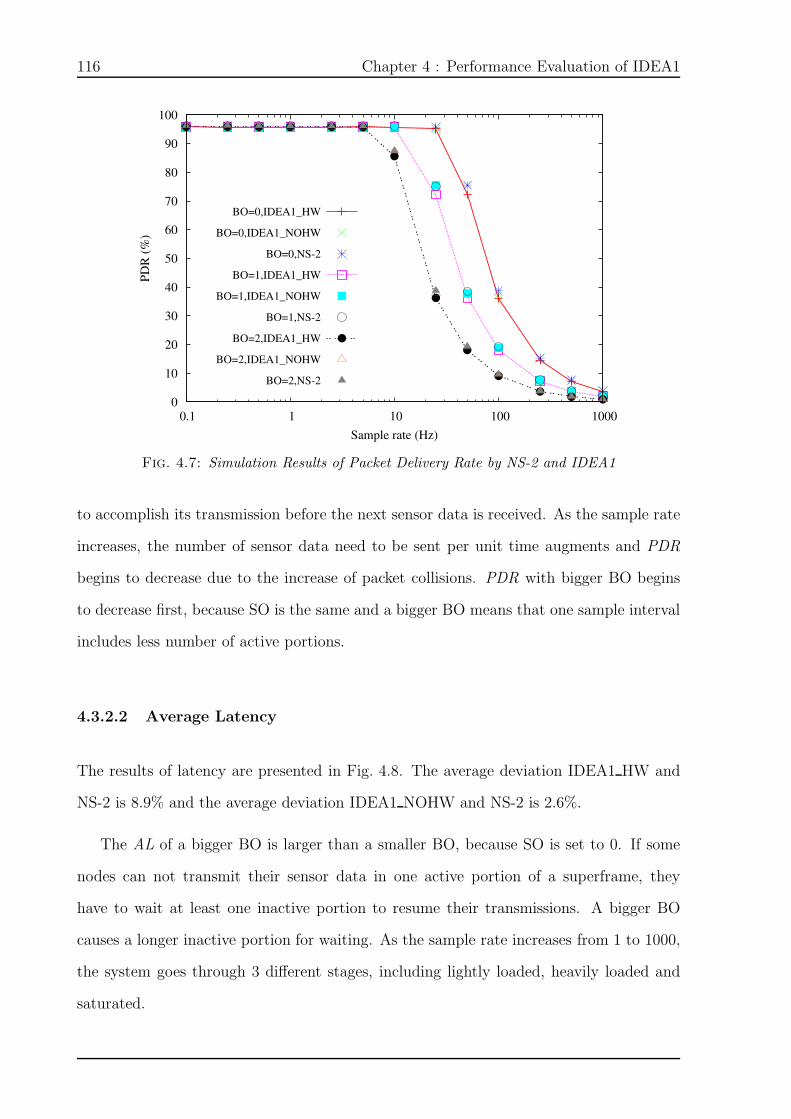
116 Chapter 4 : Performance Evaluation of IDEA1
0
10
20
30
40
50
60
70
80
90
100
0.1 1 10 100 1000
PD
R (
%)
Sample rate (Hz)
BO=0,IDEA1_HW
BO=0,IDEA1_NOHW
BO=0,NS-2
BO=1,IDEA1_HW
BO=1,IDEA1_NOHW
BO=1,NS-2
BO=2,IDEA1_HW
BO=2,IDEA1_NOHW
BO=2,NS-2
Fig. 4.7: Simulation Results of Packet Delivery Rate by NS-2 and IDEA1
to accomplish its transmission before the next sensor data is received. As the sample rate
increases, the number of sensor data need to be sent per unit time augments and PDR
begins to decrease due to the increase of packet collisions. PDR with bigger BO begins
to decrease first, because SO is the same and a bigger BO means that one sample interval
includes less number of active portions.
4.3.2.2 Average Latency
The results of latency are presented in Fig. 4.8. The average deviation IDEA1 HW and
NS-2 is 8.9% and the average deviation IDEA1 NOHW and NS-2 is 2.6%.
The AL of a bigger BO is larger than a smaller BO, because SO is set to 0. If some
nodes can not transmit their sensor data in one active portion of a superframe, they
have to wait at least one inactive portion to resume their transmissions. A bigger BO
causes a longer inactive portion for waiting. As the sample rate increases from 1 to 1000,
the system goes through 3 different stages, including lightly loaded, heavily loaded and
saturated.

Chapter 4 : Performance Evaluation of IDEA1 117
10
20
30
40
50
60
70
80
90
0.1 1 10 100 1000
Lat
ency
(m
s)
Sample rate (Hz)
BO=0,IDEA1_HW
BO=0,IDEA1_NOHW
BO=0,NS-2
BO=1,IDEA1_HW
BO=1,IDEA1_NOHW
BO=1,NS-2
BO=2,IDEA1_HW
BO=2,IDEA1_NOHW
BO=2,NS-2
Fig. 4.8: Simulation Results of Latency by NS-2 and IDEA1
During the lightly loaded stage, AL remains stable because the transmissions between
two adjacent sample intervals do not overlap; the network utilization statuses are almost
the same for different sample intervals.
When the system is heavily loaded, it is transiting to be saturated. AL increases if
B0 is not equal to SO; on the contrary, it decreases slightly if B0 is 0. In this transition
period, some nodes can not complete their transmissions before the next sample interval
begins and the last one or two nodes transmitting during the overlapping period of two
sample intervals have to compete with other seven or six nodes for channel usage. If these
last transmissions succeed, they will be longer than the case there were no overlapping
between two sample intervals and AL will increase compared with the lightly loaded

118 Chapter 4 : Performance Evaluation of IDEA1
stage; if they fail, they will not be considered in the calculation of latency and AL will
decrease. In addition, the new sensor data of the last one or two nodes will be delayed for
transmitting, which extends AL. For the case that BO is 0, there is no inactive portion
during a superframe; thus the delay of new sensor data transmissions and the extension
of old sensor data transmissions are smaller than the loss of failed transmissions of old
sensor data, as a result, AL decreases. However when BO is 1 and 2, each superframe
comprises an inactive portion, especially in case that BO is 2, the length of superframe
is 61.44 ms which includes an inactive portion of 46.08 ms; thus the delay of new sensor
data transmissions and the extension of old sensor data transmissions are larger than the
loss of failed transmissions of old sensor data, as a result, AL increases.
As the sample rate continues to increase, the system becomes completely saturated.
In these cases, all nodes always have pending sensor data to be sent and they compete
for channel usage during the active portion of every superframe. If a node gets two new
sensor data before the end of a transmission, only the last sensor data will be sent and
first ones are discarded. The delay of new sensor data transmissions is small; therefore,
AL decreases.
4.3.2.3 Average Power Consumption
Fig. 4.9 demonstrates the simulation results of APC. The average deviation IDEA1 HW
and NS-2 is 45.8% and the average deviation IDEA1 NOHW and NS-2 is 7.2%.
As the sample rate increases, APC s augments, because more sensor data need to be
sent. For a same sample rate, the power consumption of a smaller BO is larger than a
bigger BO, since a smaller BO means more beacons received and shorter inactive portion
of a superframe.
During the lightly loaded stage, APC s augments slowly. In these cases, most of the
time, the nodes are in sleep mode. When the system is heavily loaded transiting to
be saturated, sharp increase of APC s can be observed. During this period, the power

Chapter 4 : Performance Evaluation of IDEA1 119
1
10
100
0.1 1 10 100 1000
Pow
er c
onsu
mpti
on (
mW
)
Sample rate (Hz)
BO=0,IDEA1_HW
BO=0,IDEA1_NOHW
BO=0,NS-2
BO=1,IDEA1_HW
BO=1,IDEA1_NOHW
BO=1,NS-2
BO=2,IDEA1_HW
BO=2,IDEA1_NOHW
BO=2,NS-2
Fig. 4.9: Simulation Results of Power Consumption by NS-2 and IDEA1
consumptions of transmissions account for the main part of the whole power consumption.
When the system becomes completely saturated, APC s become steady which are the
largest power consumptions per node. The nodes are always in active mode during the
active portion of a superframe. Because there is no inactive portion when BO is 0, its
power consumptions are bigger than others.
4.3.2.4 Energy Consumption per Packet
Fig. 4.10 illustrates the simulation results of ECPkt. The average deviation IDEA1 HW
and NS-2 is 49.3% and the average deviation IDEA1 NOHW and NS-2 is 8.3%.
During the lightly loaded stage, ECPkt decreases as the sample rate increases and the
smallest BO consumes the most energy for a fixed sample rate. In these cases, the average
number of packets transmitted during one sample interval is the same for different sample
rates, which can be proved by the constant PDRs in Fig. 4.7; ECPkt is therefore less if the
sample interval is shorter. For a fixed sample rate, a smaller BO consumes more energy
since one sample interval includes more superframes and the nodes have to wake up to

120 Chapter 4 : Performance Evaluation of IDEA1
1
10
100
0.1 1 10 100 1000
Ener
gy/p
kt
(mJ)
Sample rate (Hz)
BO=0,IDEA1_HW
BO=0,IDEA1_NOHW
BO=0,NS-2
BO=1,IDEA1_HW
BO=1,IDEA1_NOHW
BO=1,NS-2
BO=2,IDEA1_HW
BO=2,IDEA1_NOHW
BO=2,NS-2
Fig. 4.10: Simulation Results of Energy Consumption per Packet by NS-2 and IDEA1
track the beacon packet at the beginning of each superframe.
The smallest ECPkt occurs when PDR begins to decline, where the system begins to
transit to be saturated. In this case, every node can accomplish its transmission before
new sensor data arrives, but the interval between the last node turns to sleep and the
next sensor data arrives is very short, so the nodes spend the least energy in sleep mode.
As the sample rate continues to increase, the ECPkt augments due to the transmission
overlap of two sample intervals and the increase of collisions. The energy consumption
per packet with bigger BO begins to increase first because the number of superframes per
sample interval is less for a larger BO.
When the system is saturated, ECPkt remains constant and the smallest BO consumes
the least energy. In these cases, nodes are always having pending sensor data to send. The
number of successfully transmitted packets per superframe is almost the same; therefore
ECPkt remains constant for the same BO. In addition, for a fixed sample rate, because
one superframe includes a longer inactive portion if BO is larger, its ECPkt is bigger.
Chapter 4 : Performance Evaluation of IDEA1 121
4.3.2.5 Summary
Based on the simulation results in Fig 4.7, Fig 4.8, Fig 4.9 and Fig 4.10, the deviations
of the simulation results between IDEA1_HW and NS-2 about the PDR, AL, APC and
ECPkt are 2.7%, 8.9%, 45.8% and 49.3% respectively. The ones between IDEA1_NOHW
and NS-2 are 1.0%, 2.6%, 7.2% and 8.3%. Therefore, the average deviation between
IDEA1_HW and NS-2 is 26.7%, and the one between IDEA1_NOHW and NS-2 is
4.8%. The former is bigger since more detailed information of HW/SW operations
have been considered. Especially when the sample rate is low, the deviations of
ECPkt and APC results between IDEA1 and NS-2 are very large, because the SPI
communications of microcontroller and transceiver account for a very great proportion
of the power consumptions. For example, the SPI communication takes 42.4% of the
power consumption of microcontroller when sample rate is 0.1. A more detailed power
consumption analysis of each hardware component will be provided in section 4.3.4.
4.3.3 Simulation Time of NS-2 and IDEA1
For the simulations in section 4.3, the simulation speed of IDEA1 is about 2 times faster
than NS-2. The simulation time of NS-2 and IDEA1 for the application with BO set to
2 is presented in Fig. 4.11.
The simulation of IDEA1 is IDEA1_NOHW, which is at the same abstraction level of
the IEEE 802.15.4 NS-2 model. All the simulations are executed individually on a server
with an Intel 2.66 GHz Xeon X3230 processor and a 4.6 GB memory. For the application
lasting 27.8 hours with a sample rate of 0.1 Hz, the simulation time of IDEA1 and NS-2
are 7.35 and 24.0 minutes respectively. The high speed simulation of IDEA1 profits mainly
from the efficient simulation kernel of SystemC and our optimized model implementation.
SystemC provides a wait function which can set relative processes to inactive state until
an interesting event occurs. In our model, this event interrupt mechanism is used in the
while statement of FSM implementation. Instead of checking the states of microcontroller

122 Chapter 4 : Performance Evaluation of IDEA1
1
10
100
1000
0.1 1 10 100 1000
Sim
ula
tion t
ime
(s)
Sample rate (Hz)
BO=2,IDEA1
BO=2,NS-2
Fig. 4.11: Simulation time of NS-2 and IDEA1
and transceiver every simulation cycle, their FSMs are woken up only when an interesting
event occurs, which can reduce the simulation time significantly.
4.3.4 Detailed Analysis of Power Consumptions by IDEA1
In previous sections, the fidelity of IDEA1 simulation have been proved by testbed
measurements, and the performance of IDEA1 has been compared with NS-2. In this
section, the detailed hardware modeling feature of IDEA1 is shown by a further analysis
of this application in section 4.3.
The IEEE 802.15.4 NS-2 model is at node-level. A sensor node is modeled as
a single module and no specific hardware component has been modeled. However,
IDEA1 is at component-level, both the operations of individual hardware component
and the communications among them are considered, such as SPI communication between
microcontroller and transceiver and analog to digital conversion of sensor data. The power
consumptions of hardware components in different operating modes can be investigated
by IDEA1. In this section, a complete performance evaluation of IEEE 802.15.4 sensor

Chapter 4 : Performance Evaluation of IDEA1 123
network is provided by IDEA1.
Compared to NS-2, IDEA1 can provide detailed informations about the energy
consumptions of individual hardware components. The power consumptions of hardware
components in different operating modes are also presented in Fig. 4.12.
Fig. 4.12: Power consumptions of hardware components in different operating modes
From Fig. 4.12 we can see that the average power consumption per node is bigger
when BO is 0 than BO is 2, because the nodes spend more energy for beacon tracking
when BO is 0. For a fixed BO, the power consumption per node augments as the sample
rate increases, since the nodes spend less time in sleep mode and more collision occurs. In
addition, the transceiver consumes much more energy than the microcontroller and the
energy consumed in the sleep mode is very little.
Fig. 4.13 presents the average power consumption of hardware components for different
tasks. Tracking presents the power consumed by useless beacon tracking. On receipt of a
beacon packet, if the node has no data to transmit, this beacon tracking is useless. Useful
refers to the power consumption that the useless beacon tracking is subtracted.
From Fig. 4.13, we can see that the nodes spend too much energy for useless beacon
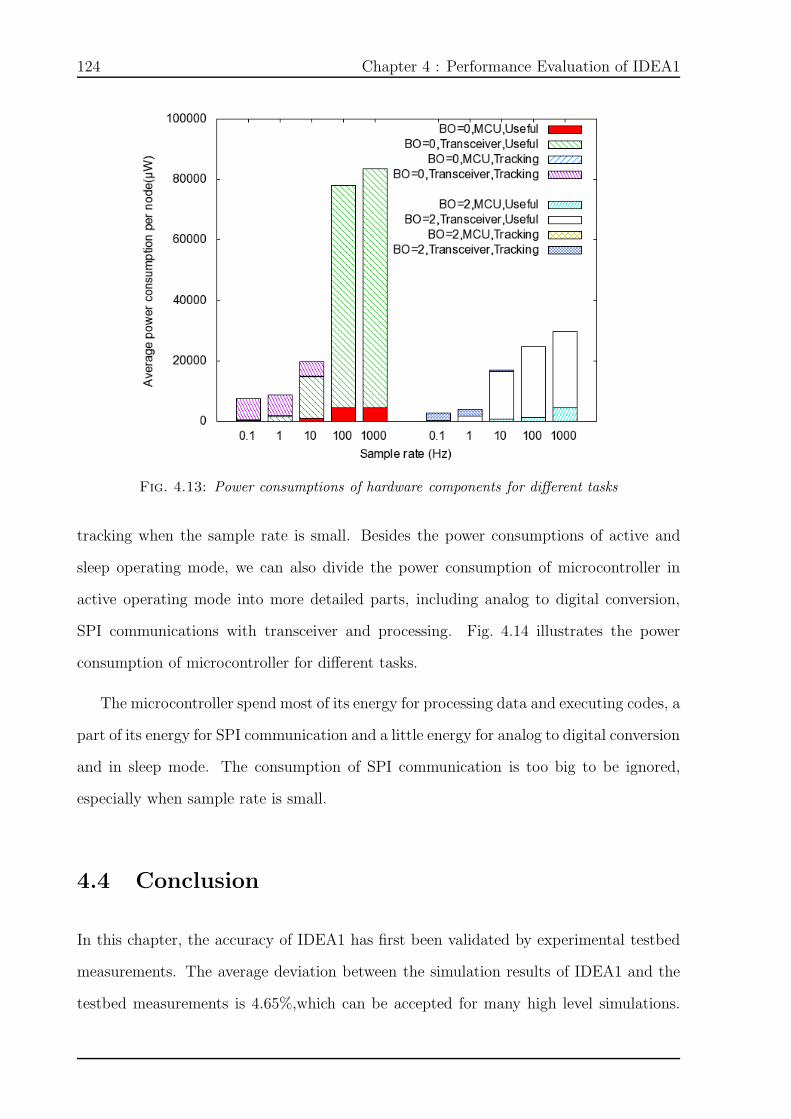
124 Chapter 4 : Performance Evaluation of IDEA1
Fig. 4.13: Power consumptions of hardware components for different tasks
tracking when the sample rate is small. Besides the power consumptions of active and
sleep operating mode, we can also divide the power consumption of microcontroller in
active operating mode into more detailed parts, including analog to digital conversion,
SPI communications with transceiver and processing. Fig. 4.14 illustrates the power
consumption of microcontroller for different tasks.
The microcontroller spend most of its energy for processing data and executing codes, a
part of its energy for SPI communication and a little energy for analog to digital conversion
and in sleep mode. The consumption of SPI communication is too big to be ignored,
especially when sample rate is small.
4.4 Conclusion
In this chapter, the accuracy of IDEA1 has first been validated by experimental testbed
measurements. The average deviation between the simulation results of IDEA1 and the
testbed measurements is 4.65%,which can be accepted for many high level simulations.

Chapter 4 : Performance Evaluation of IDEA1 125
Fig. 4.14: Power consumptions of microcontroller for different tasks
Secondly, the performances of IDEA1 have also been compared with NS-2, the most
widely used simulator in WSN research. Benefiting from the SystemC-based hardware
and software co-simulation, IDEA1 can easily model the concurrency and interconnnection
within and among hardware components. It can provide more detailed informations about
the energy consumptions than the IEEE 802.15.4 NS-2 model. Based on system-level
modeling, the simulation speed of IDEA1 is 2 times faster than NS-2.

126 Chapter 4 : Performance Evaluation of IDEA1

Chapter 5 : Case Studies 127
Chapter 5 :
Case Studies

128 Chapter 5 : Case Studies

Chapter 5 : Case Studies 129
After the experimental validation of accuracy and performance evaluation by
comparing with other simulators, IDEA1 is ready to be used in real applications. It
is firstly used to provide further performance evaluation of the IEEE 802.15.4 sensor
network studied in last chapter. The performances of this IEEE 802.15.4 are evaluated
for different parameter setting and traffic loads. Finally, IDEA1 is used to study a real
industrial application in which a wireless sensor and actuator network is deployed on a
vehicle to measure and control vibrations. By the simulation, some preliminary designs
based on IEEE 802.15.4 protocols and two different hardware platforms are evaluated.
The four metrics used in chapter 4, including PDR, AL, ECPkt and APC, are used.
This chapter is organized as follows. Section 5.1 offers a further comprehensive
performance evaluation of the IEEE 802.15.4 sensor networks studied by NS-2 and IDEA1.
Section 5.2 studies an industrial application to demonstrate the design flow and usability
of IDEA1.
5.1 Performance Evaluation of IEEE 802.15.4 Sensor
Network
A comprehensive evaluation of IEEE 802.15.4 sensor network is performed in this section.
According to the study in section 4.3, when the sample rate is small, the nodes spend too
much energy for beacon tracking without any data to send. Therefore, in this section,
we will implement the same application without beacon tracking mechanism and evaluate
the performance of this network. Until now, BO is set to 0, 1 and 2 respectively, and
SO is set to 0. Some other configurations of protocol parameters are also evaluated to
explore the maximum sample rate the IEEE 802.15.4 can support. All the simulations
are implemented on IDEA1 with considerations of hardware operation. The hardware
prototype used for this analysis is also N@L motes
The rest of this section is organized as follows. Section 5.1.1 evaluates the performance

130 Chapter 5 : Case Studies
of IEEE 802.15.4 networks in beacon-enabled mode without beacon tracking. Therefore,
in section 5.1.2, the same simulations are re-executed with SO set to the same value
with BO. Finally, in section 5.1.3 studies the IEEE 802.15.4 nonbeacon-enabled mode
and summarizes the performance evaluation of IEEE 802.15.4 LR-WPAN for industrial
applications.
5.1.1 Slotted CSMA-CA with Fixed SO and Various BO
In this section, the same application is implemented without beacon tracking mechanism
and a further analysis of this application will be presented.
5.1.1.1 Packet Delivery Rate
The simulation results of packet delivery rate are presented in Fig. 5.1.
0
10
20
30
40
50
60
70
80
90
100
0.1 1 10 100 1000
PD
R (
%)
Sample rate (Hz)
BO=0,Tracking
BO=0,noTracking
BO=1,Tracking
BO=1,noTracking
BO=2,Tracking
BO=2,noTracking
Fig. 5.1: Packet delivery rate of slotted CSMA-CA with fixed SO and various BO
In Fig. 5.1, Tracking presents the simulations of beacon tracking mechanism and
noTracking refers to the simulations without beacon tracking mechanism. The average
absolute deviation of PDR between the tracking and notracking modes is less than 0.1%
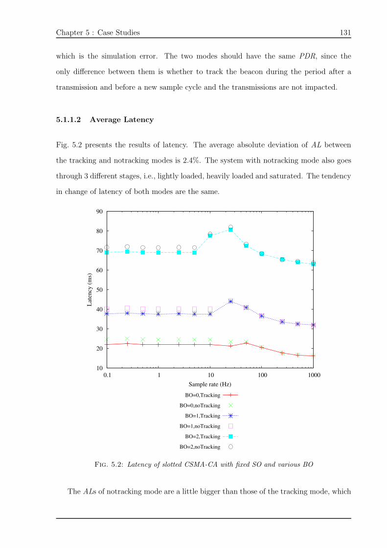
Chapter 5 : Case Studies 131
which is the simulation error. The two modes should have the same PDR, since the
only difference between them is whether to track the beacon during the period after a
transmission and before a new sample cycle and the transmissions are not impacted.
5.1.1.2 Average Latency
Fig. 5.2 presents the results of latency. The average absolute deviation of AL between
the tracking and notracking modes is 2.4%. The system with notracking mode also goes
through 3 different stages, i.e., lightly loaded, heavily loaded and saturated. The tendency
in change of latency of both modes are the same.
10
20
30
40
50
60
70
80
90
0.1 1 10 100 1000
Lat
ency
(m
s)
Sample rate (Hz)
BO=0,Tracking
BO=0,noTracking
BO=1,Tracking
BO=1,noTracking
BO=2,Tracking
BO=2,noTracking
Fig. 5.2: Latency of slotted CSMA-CA with fixed SO and various BO
The ALs of notracking mode are a little bigger than those of the tracking mode, which

132 Chapter 5 : Case Studies
is caused by the timing cost of resynchronization. With notracking mode, nodes go to
sleep mode after a transmission if they have no data to send. They wake up some time
later and performs a new sensing operation. They need to be resynchronized with the
coordinator if they want to send this new sensor data. The microcontroller wake up the
transceiver to acquire a beacon packet. During the transition from sleep to active mode
of transceiver, the coordinator may be transmitting a beacon packet. The nodes will
miss this beacon packet and they have to listen the channel for almost one superframe
duration to receive the next beacon. This resynchronization process can be observed in
the example of simulation log presented in Listing. 5.1.
Listing 5.1: Log fragment of noTracking mode
Node0 : Begin to wake up to read s enso r data at 8598154 us .
Node0 : r eads a new senso r data ( Value , Time) : 248 , 8 . 6 at 8600066 us .
Node0 : s t a r t to wake up the t r a n s c e i v e r at 8600066 us .
Transce iver 8 : s t a r t s t r ansmi t t ing the beacon at 8601600 us
Proxy 8 : Begin emitt ing rad io packet at time 8601792 us .
Proxy 8 : Complete emitt ing rad io packet at time 8602336 us .
Transce iver 0 : i s woken up at 8602066 us
Node0 : s t a r t s to transmit the data to the t r a n s c e i v e r ( NR= 0 ) with data =
248 at 8602066 us
Transce iver 0 : s t a r t s to track beacon with s t a t e = 10 at 8602066 us
Transce iver 0 : r e c e i v e s a TX packet from mi c r o c on t r o l l e r at 8602446 us .
Transce iver 8 : s t a r t s t r ansmi t t ing the beacon at 8663040 us
Proxy 8 : Begin emitt ing rad io packet at time 8663232 us .
Proxy 8 : Complete emitt ing rad io packet at time 8663776 us .
Transce iver 0 : r e c e i v e s a beacon packet and s t a r t to transmit the TX packet
at 8663776 us
Transce iver 0 : generated a random number as backo f f s l o t s , s l o t s = 3 at 8664
ms
The example shown in Listing. 5.1, BO is set to 2, corresponding to 61.44 ms
superframe. With the notracking mode, the nodes have to wake up their transceivers
after reading a new sensor data; however, during the wakeup transition of transceiver, the

Chapter 5 : Case Studies 133
coordinator has transmitted a beacon packet at 860.16 ms. The nodes have to listen to
the channel and receive a beacon packet after one superframe duration at 866.3776 ms.
If the tracking mode is used, this resynchronization will not occur. The transceiver uses
a built-in timer to count for the superframe length and wake up automatically before the
transmission of beacon packet. The same scenario of the tracking mode is illustrated in
Listing. 5.2.
Listing 5.2: Log fragment of tracking mode
Node0 : Begin to wake up to read s enso r data at 8598154 us .
Transce iver 0 : Begin to wake up to track beacon at 8599600 us .
Node0 : r eads a new senso r data ( Value , Time) : 248 , 8 . 6 at 8600066 us .
Transce iver 0 : s t a r t s to track beacon with s t a t e = 10 at 8601600 us
Node0 : s t a r t s to transmit the data to the t r a n s c e i v e r ( NR= 0 ) with data =
248 at 8601600 us
Transce iver 8 : s t a r t s t r ansmi t t ing the beacon at 8601600 us
Proxy 8 : Begin emitt ing rad io packet at time 8601792 us .
Transce iver 0 : r e c e i v e s a TX packet from mi c r o c on t r o l l e r at 8601986 us .
Proxy 8 : Complete emitt ing rad io packet at time 8602336 us .
Transce iver 0 : r e c e i v e s a beacon packet and s t a r t to transmit the TX packet
at 8602336 us
Transce iver 0 : generated a random number as backo f f s l o t s , s l o t s = 5 at
8602560 us
The beacon packet at 860.16 ms was received by the synchronized transceivers which
are woken up for tracking beacon automatically by a built-in timer. Therefore, the latency
of notraking mode is larger than that of tracking mode.
Note that the timing cost of resynchronization of the notracking mode, compared to
the tracking mode, only happens when a transmission of beacon packet occurs during the
wakeup transition of transceiver. If there is no beacon packet transmission during the
wakeup transition of transceiver, the latency results of notracking and tracking modes are
the same. In this case, the difference between these two modes is power consumption.
After reading a sensor data, the nodes of tracking mode can go to sleep again and

134 Chapter 5 : Case Studies
wake up before the transmission of beacon packet, because they know the information
of superframe. However, the nodes of notracking mode have to listen the channel until a
receipt of beacon packet.
5.1.1.3 Average Power Consumption
Fig. 5.3 demonstrates the simulation results of APC. Firstly, we analyze the change
tendency of the power consumption of notracking mode. Finally, we compare the difference
between the notracking and tracking mode.
0.1
1
10
100
0.1 1 10 100 1000
Pow
er c
onsu
mpti
on (
mw
)
Sample rate (Hz)
BO=0,Tracking
BO=0,noTracking
BO=1,Tracking
BO=1,noTracking
BO=2,Tracking
BO=2,noTracking
Fig. 5.3: Power consumption of slotted CSMA-CA with fixed SO and various BO
During the lightly loaded stage, the APC s of notracking mode increase as the sample
rate augments. In these cases, the nodes go to sleep mode after the transmission and wake
up when the next sample interval begins, so the energy spent during one sample interval
for different sample rate are almost the same. The difference of energy consumption
between two sample rates is the length of sleep mode. Therefore, the APC s increases
as the sample interval decreases. In addition, the APC of a bigger BO is higher than
that of a smaller BO, because the energy cost of resynchronization of notracking mode
for a bigger BO is more heavy. In these cases, after reading a new sensor data, the

Chapter 5 : Case Studies 135
microcontroller turns on the transceiver to listen for a beacon. The listening period is the
cost of resynchronization which can be observed in Listing. 5.1. The transceiver of Node0
is woken up at 8602066 µs which is 60974 µs before the beacon packet transmission. The
transceiver has to listen to the channel during this time. The listening period may last
long if the length of superframe is big. Finally, APC is tending towards stability when
the system is saturated. The microcontroller keeps in active mode and the transceiver
goes to sleep mode during the inactive portion of a superframe and turn to active when
active portion begins.
The APC s of notracking mode are smaller than tracking mode during the lightly loaded
stage, because one sample interval consists of a lot of superframes and the tracking mode
spends too much energy for useless beacon tracking. When the system is heavily loaded,
the APC s of notracking mode are much bigger than tracking mode. During this period,
the cost of resynchronization of notracking mode is much bigger than the useless beacon
tracking of tracking mode since one sample interval consists of a few of superframes. When
the system becomes completely saturated, the two modes have the same behaviors and
the APC s become steady.
5.1.1.4 Energy Consumption per Packet
Fig. 5.4 illustrates the simulation results of ECPkt. During the lightly loaded stage,
the ECPkts of notracking mode remain constant, because the energy spent during
one sample interval for different sample rate are almost the same and the numbers of
successfully transmitted packet during one sample interval for different sample rates are
same. While the system is heavily loaded, ECPkt begins to decrease because the cost of
resynchronization declines. Finally, ECPkt is tending towards stability when the system
is saturated.
When the sample rate is small (0.1, 0.25, 0.5, 1 and 2.5 for BO set to 1), the
ECPkts of notracking mode are smaller than the tracking mode, because the useless
beacon tracking consumes much energy. At the end of lightly loaded stage and the entire

136 Chapter 5 : Case Studies
1
10
100
0.1 1 10 100 1000
Ener
gy/p
kt
(mJ)
Sample rate (Hz)
BO=0,Tracking
BO=0,noTracking
BO=1,Tracking
BO=1,noTracking
BO=2,Tracking
BO=2,noTracking
Fig. 5.4: Energy consumption per packet of slotted CSMA-CA with fixed SO and various BO
transition stage, the ECPkts of notracking mode are bigger than the tracking mode, since
the resynchronization of notracking mode consumes much energy. When the system is
saturated, the ECPkts of notracking and tracking mode are the same. In these cases, the
system behaviors of the two modes are the same.
5.1.1.5 Summary
Based on the above analysis, we can find a best parameter setting for different sample
rates. If the sample rate is small, the notracking mode with BO set to 0 consumes the
least energy for transmitting one packet and provides the shortest AL with the best PDR.
When the sample rate is 25, the tracking mode with BO set to 0 performs better than
any other settings. If the sample rate is bigger than 25, for this application with 8 nodes
and 1 coordinator, the performance of these two modes are the same. In this period,
the contention-based CSMA-CA algorithm cannot guarantee a PDR bigger than 95% and
BO should be set to 0 in order to provide biggest PDR with shortest AL and smallest
ECPkts; however, these advantages are obtained by sustaining a big power consumption
which results a short lifetime of sensor nodes and the network.

Chapter 5 : Case Studies 137
The beacon-enabled mode without beacon tracking and with SO set to 0 has
successfully solved the useless beacon tracking problem. The ECPkts and APCs become
smaller when the sample rate is smaller. However, it still has a problem that the ALs of
a bigger BO are much longer than a smaller BO, which is caused by the waiting in the
inactive portion of a superframe because SO is set too small and some transmissions can
not be finished in one superframe. Therefore, in next section, the same simulations in this
section will be re-executed with SO set to the same value with BO.
5.1.2 Slotted CSMA-CA with Equal SO and BO
In the last section, SO is fixed to 0 and variable BO results different duty cycle in a
superframe. In this section, the application is implemented by using the beacon-enabled
slotted CSMA-CA algorithm without beacon tracking and with a SO that is equal to BO ;
the inactive portion of the superframe is thus 0. The unfinished transmissions do not have
to wait a long inactive portion for resuming. The simulation and measurement results are
presented in Fig. 5.5 and Fig. 5.6.
In order to facilitate the comparisons, the simulation results of beacon-enabled mode
without beacon tracking and with SO set 0 are also illustrated in Fig. 5.5 and Fig. 5.6.
Two improvements have been obtained if SO is set to the same value with BO. They are
presented as follows.
• PDR: PDRs with BO set to 1 and 2 are increased when the sample rate is bigger
than the start point of the stage of transition to be saturated. Because SO is equal
to BO, the nodes have more time to transmit the sensor data and the start point of
the system heavily loaded is deferred.
• AL: Latency diminishes, since the inactive portion of a superframe is set to 0 and
the nodes do not have to wait a long time for resume their transmissions in a new
superframe. During the lightly loaded stage, the ALs of a bigger BO are larger than
a smaller BO. In these cases, the nodes are in sleep mode if they have no sensor data

138 Chapter 5 : Case Studies
0
10
20
30
40
50
60
70
80
90
100
0.1 1 10 100 1000
PD
R (
%)
Sample rate (Hz)
BO=0,SO=0
BO=1,SO=BO
BO=1,SO=0
BO=2,SO=BO
BO=2,SO=0
(a) Packet Delivery Rate
10
20
30
40
50
60
70
80
90
0.1 1 10 100 1000
Lat
ency
(m
s)
Sample rate (Hz)
BO=0,SO=0
BO=1,SO=BO
BO=1,SO=0
BO=2,SO=BO
BO=2,SO=0
(b) Average Latency
Fig. 5.5: Simulated results of PDR and AL with SO equal to BO
to be sent. They will be woken up by a built-in timer if they need to read a sensor
data. In the beacon-enabled mode, the nodes can only transmit the new sensor

Chapter 5 : Case Studies 139
0.1
1
10
100
0.1 1 10 100 1000
Pow
er c
onsu
mpti
on (
mW
)
Sample rate (Hz)
BO=0,SO=0
BO=1,SO=BO
BO=1,SO=0
BO=2,SO=BO
BO=2,SO=0
(a) Average Power Consumption
1
10
0.1 1 10 100 1000
Ener
gy/p
kt
(mJ)
Sample rate (Hz)
BO=0,SO=0
BO=1,SO=BO
BO=1,SO=0
BO=2,SO=BO
BO=2,SO=0
(b) Energy Consumption per Packet
Fig. 5.6: Simulated results of APC and ECPkt with SO equal to BO
data after they successfully receive a beacon packet. We name this kind of delay of
latency is the cost of resynchronization. A sensor data may wait for a longer time to
be sent if BO is bigger. When the system is heavily loaded, the ALs become small.

140 Chapter 5 : Case Studies
As the system becomes completely saturated, the ALs of a bigger BO are shorter
than a smaller BO as a result of less receiving of beacon.
5.1.3 Unslotted CSMA-CA
The cost of resynchronization is an intrinsic drawback of beacon-enable mode; in this
section, the performance of nonbeacon-enabled mode with unslotted CSMA-CA algorithm
is thus evaluated. The simulation results are shown in Fig. 5.7 and Fig. 5.8.
The simulation results of beacon-enabled mode without beacon tracking and with SO
set 0 are also illustrated in Fig. 5.7 and Fig. 5.8. Without the cost of resynchronization, the
nonbeacon-enabled mode provides smaller ALs than beacon-enabled mode; in addition,
the ECPkts and APCs of nonbeacon-enabled mode are smaller if the system is not
saturated. However, the PDRs of nonbeacon-enabled mode are smaller than beacon-
enabled mode. Because the transmissions of nonbeacon-enabled mode are not aligned
with the backoff period boundary and CW is set to 0, the number of collisions is increased.
When the system is saturated, the ECPkts of nonbeacon-enabled mode are bigger due to
its smaller PDRs.
5.1.4 Summary
Based on the above simulations and analysis, we can find the following conclusions.
• The nonbeacon-enabled mode can provide better performance in the aspects of
latency and energy consumptions than beacon-enabled mode, but with a smaller
PDR.
• The beacon-enabled mode can offer a bigger PDR, but it has one intrinsic cost of
resynchronization which increases the latency and power consumption.
• If the sample rate is small and the system is lightly loaded, the nodes spend too
much for many useless beacon receipts if tracking is specified; thus notracking mode

Chapter 5 : Case Studies 141
0
10
20
30
40
50
60
70
80
90
100
0.1 1 10 100 1000
PD
R (
%)
Sample rate (Hz)
BO=0,SO=BO
BO=1,SO=BO
BO=2,SO=BO
nonbeacon-enabled
(a) Packet Delivery Rate
10
15
20
25
30
35
40
45
50
0.1 1 10 100 1000
Lat
ency
(m
s)
Sample rate (Hz)
BO=0,SO=BO
BO=1,SO=BO
BO=2,SO=BO
nonbeacon-enabled
(b) Average Latency
Fig. 5.7: Simulated results of PDR and AL with nonbeacon-enabed mode
should be used. In order to minimize the impact of the resynchronization cost, BO
is set to 0.
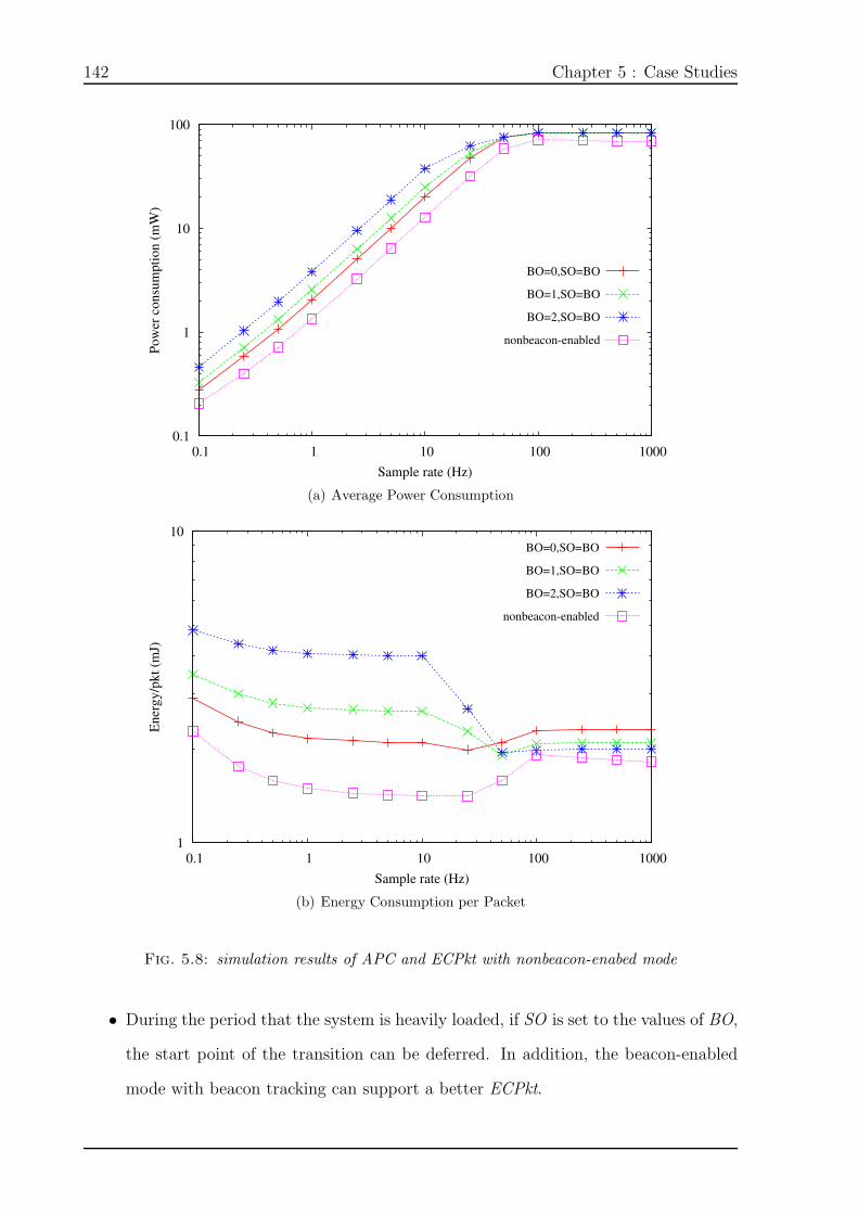
142 Chapter 5 : Case Studies
0.1
1
10
100
0.1 1 10 100 1000
Pow
er c
onsu
mpti
on (
mW
)
Sample rate (Hz)
BO=0,SO=BO
BO=1,SO=BO
BO=2,SO=BO
nonbeacon-enabled
(a) Average Power Consumption
1
10
0.1 1 10 100 1000
Ener
gy/p
kt
(mJ)
Sample rate (Hz)
BO=0,SO=BO
BO=1,SO=BO
BO=2,SO=BO
nonbeacon-enabled
(b) Energy Consumption per Packet
Fig. 5.8: simulation results of APC and ECPkt with nonbeacon-enabed mode
• During the period that the system is heavily loaded, if SO is set to the values of BO,
the start point of the transition can be deferred. In addition, the beacon-enabled
mode with beacon tracking can support a better ECPkt.

Chapter 5 : Case Studies 143
• When the system is completely saturated, the PDRs of the CSMA-CA algorithms
are less than 50% and a bigger BO with SO set to its value can provide a better
performance in the aspects of both latency and energy consumption.
5.2 An Industrial Application
In this section, IDEA1 is used to study an industrial application of WSN in vibration
measurement in order to validate and demonstrate the usability of IDEA1 in the real
project.
WSNs have recently received much attention in the industrial communications
community [137]. An important class of applications is monitoring the equipment and
machinery health, using for example vibration, heat or thermal sensors. Our group
participated in a project, named Mechanic@Lyon (M@L) [136]. It is a project supported
by Ingenierie@Lyon (I@L), an institute of Carnot Network. The objective of this project is
to identify and integrate some new intelligent control technologies in automotive systems
in order to improve the internal comfort (reduce the vibration and noise). A wireless
sensor and actuator network is deployed on an automobile to measure and control its
vibration.
The first task of our work is to design the sensor network from the network protocol to
the hardware specifications of each component on a sensor node. At the beginning, some
preliminary designs based on several existing hardware platforms and communication
protocols need to be investigated at an early stage.
The rest of this section is organized as follows. Firstly, section 5.2.1 introduces
the industrial application. Secondly, section 5.2.2 studies this application by analytical
methods. Finally, section 5.2.3 presents the simulation results of IDEA1.

144 Chapter 5 : Case Studies
5.2.1 Introduction to the Industrial Application
The architecture of sensor and actuator network is shown in Fig. 5.9. This sensor network
is composed of several nodes and a coordinator. The nodes measure periodically the
vibrations of their given positions by a piezoelectric sensor and transmit the data to a
coordinator which collects the sensor data of all nodes. A sample occupies one byte. The
coordinator is connected to a host that analyzes the collected data and implements control
algorithms by an actuator network. The main challenges of designing this sensor network
are the high sample rate and real-time requirements. The node should read the sensor
data with a sample rate exceeding kilohertz and send the data to the coordinator within
a short latency.
Fig. 5.9: M@L wireless sensor and actuator network infrastructure
At the early stage, some preliminary designs based on the existing hardware platforms
and network protocols need to be evaluated. Four metrics, including PDR, AL, ECPkt
and APC, are used to evaluate the network performance.
The performance of IEEE 802.15.4 [15] protocol is first evaluated since it has been
widely used in the real time industrial automations [138]. In next section, some
preliminary analysis are made in order to obtain a first understanding of this application.

Chapter 5 : Case Studies 145
In section 5.2.3, both the CSMA-CA and GTS algorithms are evaluated by simulations.
Two sensor nodes that support the IEEE 802.15.4 standard, MICAz and N@L, are
chosen as the hardware platforms. These two sensor platforms have been introduced
in section 2.2.2 and section 3.2.3.
5.2.2 Preliminary Study
In this section, some preliminary analysis are provided based on some existing works on
the performance analysis of the IEEE 802.15.4 standard. At first, the eight nodes deployed
on the vehicle roof are modeled. The nodes and coordinator form a star topology, where
all nodes can communicate with the coordinator directly. The nodes store the sample
data temporarily in a data buffer and they will send the sensor data to the coordinator
if the data in the buffer is more than sizePayload bytes. sizePayload is the payload field
length of data packet.
As shown by the simulation results of IEEE 802.15.4 protocols in section 5.1, the
PDRs of the CSMA-CA algorithms are very small when the sample rate is 1 kHz, because
they are based on the random backoff mechanism and contention-based channel access.
In addition, the mathematical analysis in [139] [140] proves that the unslotted and slotted
CSMA-CA algorithms can not guarantee a 100% packet delivery rate and the channel
access success probability decreases monotonically when the number of nodes is bigger
than one, since the number of nodes competing for the channel increases.
As stated in section 2.3.2.3, the contention free guaranteed time slots algorithm is
design to support applications with particular latency requirements. The studies made
in [141] showed that the minimum latency of IEEE 802.15.4 GTS algorithm is 15.9 ms
for any star network of any size, since the IEEE 802.15.4 standard requires a minimum
length of CAP period that is 440 symbols (7.04 ms).
Besides the limited minimum latency of the IEEE 802.15.4 GTS algorithm, another
constraint of this algorithm is that the maximum number of GTSs in a superframe is set

146 Chapter 5 : Case Studies
to 7. Since our application consists of 8 nodes, a TDMA-based GTS algorithm proposed
in [138] is adopted. It is more suitable for industrial applications which require low packet
delivery latency. It makes some modifications to the IEEE 802.15.4 GTS algorithm and
these modifications can be easily implemented by software on the two hardware platforms
we use. The contention access period (CAP) is set to 0. The contention free period (CFP)
is divided into 8 equal parts, called node slot, which are allocated to nodes off-line. During
its slot, the node wakes up if it has data to transmit. Transmissions do not require ACKs
since they happen during GTSs without contention. The node tracks the beacon at the
beginning of every superframe. It starts transmitting within its GTS that is allocated
beforehand. The node is in SLEEP mode when it is not transmitting data or receiving
beacon packets. The structure of this superframe is presented in Fig 5.10.
Fig. 5.10: Superframe structure for the TDMA-based GTS algorithm
The sample data is presented as a short integer type with one byte. The data frame
format has been presented in Fig. 3.4. Because all the nodes can reach the coordinator
directly and the number of nodes is 8, we use the short address with two bytes to identify
the nodes and coordinator, and the data frame only includes one address, either the source
address or the destination address. For a packet from a node to the coordinator, the value
in the address field is the source address so that the coordinator can identify the packet is
from which node; for a packet from the coordinator to the nodes, the destination address
is loaded in the address field of the data frame so that the right node can receive this
packet. In this context, the maximal size of payload field can attain 121 bytes, since the
maximal value of the frame length field is 127 bytes. The frame length, frame control,
sequence number and address fields occupy 6 bytes. The data fame structure is presented
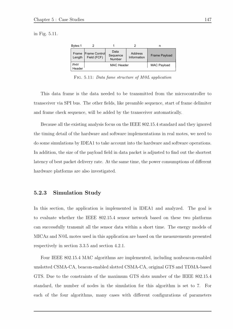
Chapter 5 : Case Studies 147
in Fig. 5.11.
Fig. 5.11: Data fame structure of M@L application
This data frame is the data needed to be transmitted from the microcontroller to
transceiver via SPI bus. The other fields, like preamble sequence, start of frame delimiter
and frame check sequence, will be added by the transceiver automatically.
Because all the existing analysis focus on the IEEE 802.15.4 standard and they ignored
the timing detail of the hardware and software implementations in real motes, we need to
do some simulations by IDEA1 to take account into the hardware and software operations.
In addition, the size of the payload field in data packet is adjusted to find out the shortest
latency of best packet delivery rate. At the same time, the power consumptions of different
hardware platforms are also investigated.
5.2.3 Simulation Study
In this section, the application is implemented in IDEA1 and analyzed. The goal is
to evaluate whether the IEEE 802.15.4 sensor network based on these two platforms
can successfully transmit all the sensor data within a short time. The energy models of
MICAz and N@L motes used in this application are based on the measurements presented
respectively in section 3.3.5 and section 4.2.1.
Four IEEE 802.15.4 MAC algorithms are implemented, including nonbeacon-enabled
unslotted CSMA-CA, beacon-enabled slotted CSMA-CA, original GTS and TDMA-based
GTS. Due to the constraints of the maximum GTS slots number of the IEEE 802.15.4
standard, the number of nodes in the simulation for this algorithm is set to 7. For
each of the four algorithms, many cases with different configurations of parameters

148 Chapter 5 : Case Studies
(e.g., sizePayload, superframe length, macMaxCSMABackoffs, macMaxFrameRetries,
etc.) have been simulated. Since the sample rate is constant, a small sizePayload results in
more packets to be sent, causing more collisions and thus lower PDR. In contrast, a large
sizePayload leads a longer time for transmitting a packet, which increases the possibilities
of channel access failures and causes lower PDR too. The best PDR, hence, occurs in the
case with a moderate sizePayload. However, sizePayload should be as short as possible.
A smaller sizePayload means the first sensor data in the packet need to wait a shorter
time to be sent. Here only the best result with the highest PDR (or lowest AL if two or
more cases achieve the biggest PDRs) is presented. Each case includes 2500 samples and
is simulated 100 times with different seeds of the random number generator of backoff
periods. The simulation results of MICAz and N@L motes are provided in Table 5.1.
Tab. 5.1: Simulation results of Of MICAz and N@L motes
Algorithm Unslotted CSMA-CA Slotted CSMA-CA IEEE802154 GTS TDMA-based GTSHardware platform MICAz N@L MICAz N@L MICAz N@L MICAz N@LsizePayload (byte) 30 30 30 30 30 15 10 19
BO n/a n/a 1 1 1 0 n/a n/aBI (µs) n/a n/a 30720 30720 30720 15360 10000 19000PDR (%) 36.5 54.4 39.7 67.4 97.4 97.4 100 100AL (µs) 11583 15841 22426 24250 53854 42777 6953 12508
ECPkt (µJ/pkt) 3811 1924 3784 1576 1283 1001 425 408APC (µW) 46693 35155 50397 35684 41071 64630 42300 21264
APC of microcontroller (µW) 29916 4576 29916 4576 29915 4448 29928 4573APC of transceiver (µW) 16777 30579 20481 31108 11157 60182 12371 16691
5.2.3.1 Comparisons of MAC algorithms
The CSMA-CA algorithms are not appropriate for this industrial application due to the
low PDRs, which is caused by the large number of collisions. The sample rate is too high
that the system is overloaded.
For the original IEEE 802.15.4 GTS algorithm, because the packet is transmitted
after the CAP portion (at least 7.04 ms), the AL is high. During one superframe of 30.72
ms, 30.72 sensing operations are performed, but only 30 sensor data can be sent in one
packet; the PDRs can not therefore be 100%. This algorithm is implemented by software
in MICAz and by hardware in N@L. For MICAz mote, after receiving a beacon packet,

Chapter 5 : Case Studies 149
the microcontroller can set the transceiver to sleep mode until its GTS slot; however for
N@L mote, the transceiver performs automatically and stays in active mode during the
CAP portion of a superframe. Therefore, the power consumption of this algorithm based
on N@L motes is much bigger than that of MICAz motes.
For the TDMA-based GTS algorithm, the PDRs can attain 100%, which prove that
the TDMA-based GTS algorithm can reliably transmit the sensor data to the coordinator.
However, this IEEE 802.15.4 sensor network fails to meet the real-time requirement of this
application. Although the average latency of packets can attain 7.0 ms, sizePayload is 10
samples which mean that the first sample data should wait 17 ms to be received by the
coordinator. This latency of sensor data is too high to generate a real-time control action.
5.2.3.2 Comparisons of Hardware Platforms
The PDRs of N@L are bigger than MICAz, because the MAC algorithms are implemented
in MRF24J40 by hardware and the sensing operation in PIC16LF88 has limited impact on
the communication process. For N@L mote, the communication process in transceiver and
the sensing operation (analog to digital conversion) in microcontroller can be performed
at the same by these two hardware components; however, the microcontroller of MICAz
mote has to stop its task immediately when the sensing timer expires.
The ALs of N@L is larger than MICAz, since for transmitting a same data frame
the SPI communication between PIC16LF88 and MRF24J40 is longer than that between
ATMEL ATMega128 and TI CC2420. In order to transmit one packet of several bytes
from PIC16LF88 to MRF24J40, the address needs to be sent before each byte. However,
ATMega128 only has to transmit one address for a whole packet.
Microchip PIC16LF88 is a power-efficient microcontroller. With a extra low power
consumption microcontroller, the APC s of N@L is smaller than MICAz, although the
power consumption of MRF24J40 is much higher than CC2420. CC2420 provides an
IDLE state that is power saving. When it is not receiving or transmitting, it will be at

150 Chapter 5 : Case Studies
IDLE state. However, MRF24J40 does not support an IDLE state. Except transmitting,
the transceiver is at RX state which is energy consuming.
5.2.3.3 Detailed Analysis of Energy Consumption
Besides the global results about the performances at network level presented in Table 5.1,
some detailed analysis about the energy consumption at hardware component level are
also provided, as presented in Fig. 5.12.
Uns
lotted
Slo
tted
IEE
E G
TS
TD
MA
GT
SU
nslo
tted
Slo
tted
IEE
E G
TS
TD
MA
GT
S
MICAz N@L
Fig. 5.12: An energy breakdown at component level
In Fig. 5.12, the energy consumption of a node is broken down into many small
parts, including consumptions of microcontroller and transceiver. The main operations of
microcontroller is composed of analog to digital conversion, SPI communication and data
processing. For the transceiver, we have chosen to separate the energy consumption in
two parts : consumption in active mode and consumption in sleeping mode.
From Fig. 5.12, we can find that the energy consumption of ATEMega128 (yellow

Chapter 5 : Case Studies 151
part) is much more than that of PIC16LF88. The latter is more power-efficient. In
addition, the analog to digital conversion of PIC16LF88 (66µs) is short than that of
ATEMega128 (219µs). However, the transceiver of N@L mote, MRF24J40, is much more
power consuming than that CC2420, the transceiver of MICAz mote. Compared with
other algorithms and configurations, the energy consumption of MRF24J40 with the IEEE
GTS algorithm is very large, because this algorithm is implemented by hardware and the
transceiver stays on active after receiving a beacon packet until its GTS slot. On the
contrary, more flexibility can be obtained by the software implementation of this algorithm
on MICAz and the microcontroller can set the transceiver to sleep mode after the receipt
of a beacon and wake it up before the allocated GTS slot.
5.3 Conclusion
In this chapter, IDEA1 has been used in two case studies to demonstrate its usability and
design flow. First, the performance of IEEE 802.15.4 sensor network has been evaluated
by IDEA1 simulations. The advantages and disadvantages of different algorithms with
various parameter settings for different traffic loads have been summarized. Finally,
IDEA1 has been used to design a real-time industrial application in which a wireless
sensor and actuator network is deployed on a vehicle to measure and control vibrations.
The best configurations of protocol parameters for various traffic loads based on different
hardware platforms have been identified. By these two case studies, the usability of IDEA1
in real development of WSN systems has been demonstrated. IDEA1 can help the system
designers to evaluate some primary designs with low timing and financial cost at an early
stage of design flow. It is able to explore the design space by tuning the parameters of
both sensor nodes and network protocols.

152 Chapter 5 : Case Studies

Chapter 6 : Conclusions and Future Works 153
Chapter 6 :
Conclusions and Future Works

154 Chapter 6 : Conclusions and Future Works

Chapter 6 : Conclusions and Future Works 155
6.1 Summary of Work
This thesis has investigated the modeling and simulation of wireless sensor networks.
A validated SystemC-based system-level design and simulation environment for WSN
systems, named IDEA1, has been developed.
Based on the SystemC-based support of modeling concurrency, structural hierarchy,
interrupts and synchronization primitives of embedded systems, IDEA1 enables the
hardware and software co-simulation of wireless sensor networks. By doing this, the
energy consumptions of an individual sensor node and the whole network can be
accurately predicted. The energy model implemented in IDEA1 takes into account the
power consumptions of all operation modes of each hardware component and transitions
between different modes. IDEA1 implements a clock-based synchronization mechanism
to provide performance evaluation with cycle accurate communication and approximate
time computation. Many off-the-shelf hardware components, such as MICAz and MICA2,
are modeled. The IEEE 802.15.4 standard is implemented.
Firstly, the simulation results of IDEA1 were compared with some experimental
measurements on a testbed of 9 nodes in the aspects of packet delivery rate, average
latency, energy consumption per packet and average power consumption. The average
deviation between the IDEA1 simulations and the experimental measurements is 4.6%
which can be accepted by general system-level simulations. The performances of IDEA1
have also been compared with NS-2, the most widely used simulator in WSN research.
Benefiting from the SystemC-based hardware and software co-simulation, IDEA1 provides
more detailed information about the energy consumptions than NS-2. If the timing
information of some relative hardware operations are not considered in IDEA1, the average
deviation between IDEA1 and NS-2 simulations is 4.8% which proves that IDEA1 can
provide the same accuracy with NS-2. However, if the relative hardware operations
are considered in the IDEA1 simulation, the average deviation between IDEA1 and
NS-2 simulations is 26.7%. Especially when the sample rate is low, the deviations of

156 Chapter 6 : Conclusions and Future Works
energy consumption results between IDEA1 and NS-2 are very large, because the SPI
communications between microcontroller and transceiver and other hardware operations
account for a very great proportion of the power consumptions. Based on system-level
modeling, the simulation speed of IDEA1 is 2 times faster than NS-2.
Finally, two case studies have been performed to show the usability and design flow
of IDEA1. The performance of IEEE 802.15.4 sensor network was comprehensively
evaluated. For various traffic loads, diverse configurations of protocol parameters,
including unslotted and slotted CSMA/CA algorithms and different superframe
architectures are simulated. In addition, a real-time active vibration control application
was also studied. By the simulation studies of IDEA1, the best choice of communication
protocols based on MICA2 or N@L motes was found.
6.2 Future Works
The research work implemented for this thesis has successfully met the research
motivations proposed in section 1.2. However, the investigated research area of modeling
and simulation of wireless sensor networks has been highlighted as a diverse aspect of
WSNs. There are many additional research that could be conducted to further this
research.
• To enhance the capability of IDEA1 in modeling the real WSN systems, some typical
sensor chips need to be modeled by SystemC.
• Operating system is one important part of the software development for WSN
system; therefore IDEA1 will be more powerful if it can provide operating system
abstraction supports. In addition, more accurate software modeling techniques, such
as instruction set simulation, will be investigated.
• The simulation of IEEE 802.15.4 sensor networks showed that this standard is
more efficient for low duty cycle applications; therefore, for some high sample rate

Chapter 6 : Conclusions and Future Works 157
applications, more communication protocols, especially high data rate protocols,
need to be investigated.
• The protocols of high layers, such as network and transport layers, should be
implemented so as to enable the large scale sensor network simulation and design.
• The radio propagation models in current version of IDEA1 only contains two typical
application scenarios. Some more accurate and complex propagation models should
be implemented in IDEA1.
• The battery discharge model in current version of IDEA1 is only a linear one. Some
more accurate models need to be investigated.

158 Appendix A. Modifications to the IEEE 802.15.4 NS-2 Model
Appendix A. Modifications to the IEEE 802.15.4 NS-2 Model 159
Appendix A :
Modifications to the IEEE 802.15.4
NS-2 Model

160 Appendix A. Modifications to the IEEE 802.15.4 NS-2 Model

Appendix A. Modifications to the IEEE 802.15.4 NS-2 Model 161
When comparing the performances of IDEA1 with NS-2, we utilized the IEEE 802.15.4
NS-2 model in release 2.34 [24] and [25]. The existing IEEE 802.15.4 NS-2 model has been
modified, since it was built complying with an earlier standard edition (IEEE 802.15.4
draft D18), which has been nowadays replaced by the latest revised release IEEE Std
802.15.4-2006 [15]. In addition, some bugs have been fixed and several new functions have
been added. The main modifications are listed as follows.
1. Add function ”sendData(IE3ADDR SrcAddr,IE3ADDR DstAddr,UINT 8 pay-
loadLength,bool isUperlayer)” in the p802 15 4sscs class. Users can call this function
to send data to the MAC layer in the tcl script.
2. Add function ”MCPS DATA confirm(UINT 8 msduHandle,MACenum status)” in
the p802 15 4sscs class. This function is used by the MAC layer to report the
transmission results to the SSCS layer. On receipt of this report, the MAC layer
can start next transmission.
3. Add function ”MLME BEACON NOTIFY indication(UINT 8 BSN,PAN ELE
*PANDescriptor,UINT 8 PendAddrSpec,IE3ADDR *AddrList,UINT 8
sduLength,UINT 8 *sdu)” in the p802 15 4sscs class. This function is used
by the MAC layer to report the successful receipt of a beacon packet so that
the SSCS layer knows when the CAP ends. During the inactive portion of the
superframe, the ”sendData” function can not be invoked.
4. Disable ”if ((!mpib.macAutoRequest)||(wph->MSDU PayloadLen > 0))” in the
function ”recvBeacon(Packet *p)” of p802 15 4mac to enable the SSCS layer to
handle the beacon transmission event.
5. Enable the first ”log(p->refcopy());” in the ”recvData(Packet *p)” function and
disable the first ”log(msdu->refcopy());” in the ”MCPS DATA indication” function
of p802 15 4mac so as to log a packet in the trace file immediately when the node
receives the packet, but not after sending the ACK.

162 Appendix A. Modifications to the IEEE 802.15.4 NS-2 Model
6. Change ”if(newtime > 0.0)” to ”if(newtime > 0.0000000001)” in ”locateBound-
ary(bool parent,double wtime)” function of p802 15 4mac, because newtime is a
double variable, when it is 0, in fact, it is a small value that is bigger than 0
and less than 0.0000000001.
7. According to the IEEE 802.15.4 standard-2006, after backoff, if the CSMA algorithm
can not proceed the following process in this CAP, it should wait to the next
superframe and redo the backoff. Add ”start (false);” in the ”newBeacon(char trx)”
function of p802 15 4csmaca.
8. Add ”rxCmd = 0;” in the ”if ((frmCtrl.frmType == defFrmCtrl Type MacCmd) &&
(wph->MSDU CmdType == 0x01))”statement of the ”recv(Packet *p, Handler *h)”
function of p802 15 4mac in order to solve the problem that some devices can not
associate with the coordinator because the BSY drop packet. If the beacon timer
expires when the coordinator is sending ACK for the CM4 command to a node, the
coordinator has to send beacon immediately. In this case, the rxCmd packet should
be cleared, so that when that a device sends a new CM4 command, the coordinator
will not drop it by checking ”rxCmd!=0”.
9. Change ”if ((rxCmd)||(txBcnCmd))” to ”if (rxCmd )” in the ”recv(Packet *p,
Handler *h)” function of p802 15 4mac in order to solve the problem that some
devices can not associate with the coordinator because the BSY drop packet. If
the beacon timer expires when the coordinator is waiting an ACK for the CM2
command, the coordinator is forced to send beacon immediately. In this case, the
txBcnCmd packet has not been cleared, so when nodes send a new CM4 command
in the next superframe, the coordinator will drop it by checking ”txBcnCmd!=0”.
With this modification and the last one, the BSY error becomes rare, but I can not
remove it totally. It happens randomly to some simulations. Maybe there are still
some cases I did not discover. To guarantee the correctness of my simulations only
concerning the communication process after the association stage, I check the trace

Appendix A. Modifications to the IEEE 802.15.4 NS-2 Model 163
file of every simulation. If there are some devices not successfully associated, I will
redo that simulation.
10. Change ”delay = locateBoundary((p802 15 4macDA(txAck) ==
mpib.macCoordShortAddress),0.0);” to ”delay = 0.0;” in the
”PLME SET TRX STATE confirm(PHYenum status)” function of p802 15 4mac.
The transmission of an acknowledgment frame in the CAP period shall commence
either aTurnaroundTime symbols after the reception of the last symbol of the data
or MAC command frame or at a backoff slot boundary. I chose to use the first case.
11. Disable ”reset();” in the ”newBeacon ()” function of p802 15 4csmaca. In a new
superframe, the CSMA-CA algorithm does not need to reset. It will continue the
operation in the last superframe. For example, if NR is 2 in at the end of last
superframe, at the beginning of new superframe, NR is still 2 and does not need to
reset to 0.
12. Some modifications in mcps data request() of p802 15 4mac.cc to set the format of
sending packet.
13. Replace the ”canProceed()” function of p802 15 4csmaca by a modified function
made by Ca Phan on ”http://mailman.isi.edu/pipermail/ns-developers/2007-
July/003196.html”. The reason is ”First, we can not use UINT 16 for
t bPeriods,t CAP. Because the values of t CAP (in abackoffperiodunit) will exceeds
the maximum value of 16bits number for SO>=11. For instance, when SO=11, then
t CAP= 98304 (abackoffperiodunits) > 65535 (maximum value of 16bits). Hence,
in this function, we have to use UINT 32 instead of UINT 16. Second, when this
function calculates the bPeriodsLeft, an fundamental error occurs when the packet
arrives in the off period. In this case, the bPeriodsLeft get a wrong value.”.
14. Two further modifications have been implemented in the new modified
”canProceed()” function of p802 15 4csmaca.

164 Appendix A. Modifications to the IEEE 802.15.4 NS-2 Model
t bPeriods sometimes is -1998362383. It is caused by ”t CAP = (UINT 32)
(tmpf / phy->getRate(’s’));”. Converting to end of CAP to an integer caused many
errors.
With ”t transacTime += phy->trxTime(txPkt); t transacTime += mac-
>mpib.macAckWaitDuration / phy->getRate(’s’);”, the txPkt time has been added
to t transacTime, but with ”macAckWaitDuration=phy->trxTime(txPkt)+phy-
>trxTime(ACKPkt),”, the txPkt time is calculated again.
15. Add the modifications of Iyappan, who has added the sleep mode to nodes.
16. Add sensing time information in the timestamp field of pkt so as to measure the
average latency of sensor data.
17. Add macBeaconSOTimer in ”p802 15 4mac” class to set nodes to sleep after the
active portion.
18. Add ”status =SLEEP;” in the ”putNodeToSleep();” function and ”status =IDLE;”
in the ”wakeupNode(void).” function of Phy802 15 4. The energy is updated during
channel sleep time . Maybe it is cause by the incompatibility between Iyappan’s
code (based on release 2.28) and release 2.34.
19. Add ”#define NONBEACON ” in the ”p802 15 4phy.h” file to set the network
to Nonbeacon-enabled mode (do not check if it is during CAP of a superframe
in sendData of SSCS802 15 4 and do not setWakeTimer in putNodeToSleep of
p802 15 4phy).
20. Add ”mac->phy->putNodeToSleep();” in the ”MCPS DATA confirm” function of
SSCS802 15 4 to set nodes to sleep if the transmission finishes and no data to
transmit. In addition, add ”mac->phy->wakeupNode();”in the ”sendData” function
of SSCS802 15 4 to wake nodes up if they are in SLEEP.
21. Change ”node()->energy model()->DecrSleepEnergy(NOW-channel sleep time ,
P sleep );” to ”node()->energy model()->DecrSleepEnergy(NOW-

Appendix A. Modifications to the IEEE 802.15.4 NS-2 Model 165
update energy time , P sleep );” in the ”wakeupNode()” function of Phy802 15 4.
The UpdateSleepEnergy() function is invoked every second if the sleep interval
is bigger than 1s, so the DecrSleepEnergy function will decrease more energy,
including the energy that has been decreased UpdateSleepEnergy().
22. Add ”node()->energy model()->DecrIdleEnergy(NOW-update energy time ,
P idle );” in the ”putNodeToSleep” function of Phy802 15 4 to decrease the energy
consumed from the last update energy time to NOW.

166 Bibliography
Bibliography
[1] D. Bri, M. Garcia, J. Lloret, and P. Dini, “Real deployments of wireless sensor
networks,” Proc. of the 3rd int. conf. on Sensor Technologies and Applications, pp.
415–423, 2009.
[2] J. Yick, B. Mukherjee, and D. Ghosal, “Wireless sensor network survey,” Computer
Networks, vol. 52, no. 12, pp. 2292 – 2330, 2008.
[3] G. Sachdeva, R. Domer, and P. Chou, “System modeling: A case study on a wireless
sensor network,” University of California, Irvine, Tech. Rep. CECS-TR-05-12, 2005.
[4] F. Fummi, D. Quaglia, and F. Stefanni, “A systemc-based framework for modeling
and simulation of networked embedded systems,” in Proc. of the Forum on
Specification and Design Languages, 2008, pp. 49–54.
[5] K. Virk, K. Hansen, and J. Madsen, “System-level modeling of wireless integrated
sensor networks,” in Proc. of the Int. Symposium on System-on-Chip, 2005, pp.
179–182.
[6] J. Hiner, A. Shenoy, R. Lysecky, S. Lysecky, and A. G. Ross, “Transaction-level
modeling for sensor networks using systemc,” in Proc. of the 2010 IEEE int.
conf. on Sensor Networks, Ubiquitous, and Trustworthy Computing, ser. SUTC ’10.
Washington, DC, USA: IEEE Computer Society, 2010, pp. 197–204.
[7] M. Damm, J. Moreno, J. Haase, and C. Grimm, “Using transaction level modeling
techniques for wireless sensor network simulation,” in Proc. of the Conference on
Design, Automation and Test in Europe, ser. DATE ’10, 2010, pp. 1047–1052.
[8] S. Kurkowski, T. Camp, and M. Colagrosso, “Manet simulation studies: the
incredibles,”SIGMOBILE Mob. Comput. Commun. Rev., vol. 9, pp. 50–61, October
2005.
[9] IEEE Std 1666 - 2005 IEEE Standard SystemC Language Reference Manual,
Institute of Electrical and Electronics Engineers, 2006.
[10] Information technology – Open Systems Interconnection – Basic Reference Model:
The Basic Model, Institute of Electrical and Electronics Engineers Std., 1994.
[11] ZigBee specification - Document 053474r17, ZigBee Alliance, 2007. [Online].
Available: http://www.zigbee.org/

Bibliography 167
[12] I. F. Akyildiz, W. Su, Y. Sankarasubramaniam, and E. Cayirci, “Wireless sensor
networks: a survey,”Computer Networks, vol. 38, no. 4, pp. 393–422, 2002. [Online].
Available: http://dblp.uni-trier.de/db/journals/cn/cn38.html#AkyildizSSC02
[13] W. Ye, J. Heidemann, and D. Estrin, “An energy-efficient mac protocol for wireless
sensor networks,” in Proc. of the Joint Conference of the IEEE Computer and
Communications Societies (InfoCom), USC/Information Sciences Institute. New
York, NY, USA: IEEE, June 2002, pp. 1567–1576.
[14] K. K. II and P. Mohapatra, “Medium access control in wireless sensor networks,”
Computer Networks, vol. 51, no. 4, pp. 961 – 994, 2007.
[15] IEEE Standard for Information technology- Telecommunications and information
exchange between systems- Local and metropolitan area networks- Specific
requirements Part 15.4: Wireless Medium Access Control (MAC) and Physical
Layer (PHY) Specifications for Low-Rate Wireless Personal Area Networks
(WPANs), Institute of Electrical and Electronics Engineers, 2006.
[16] ATMEL ATMega128 datasheet, Atmel Corporation. [Online]. Available: www.
atmel.com/atmel/acrobat/doc2467.pdf
[17] TI CC2420 datasheet, Texas Instruments Incorporated. [Online]. Available: focus.
ti.com/lit/ds/symlink/cc2420.pdf
[18] PICmicro Mid-Range MCU Family Reference Manual, Microchip Technology Inc.
[Online]. Available: ww1.microchip.com/downloads/en/devicedoc/33023a.pdf
[19] Microchip MRF24J40 Data Sheet, Microchip Technology Inc. [Online]. Available:
ww1.microchip.com/downloads/en/DeviceDoc/DS-39776b.pdf
[20] G. P. Halkes and K. G. Langendoen, “Experimental evaluation of simulation
abstractions for wireless sensor network mac protocols,” EURASIP J. Wirel.
Commun. Netw., vol. 2010, pp. 24:1–24:2, April 2010.
[21] G. V. Merrett, N. M. White, N. R. Harris, and B. M. Al-Hashimi, “Energy-
aware simulation for wireless sensor networks,” in Proc. of the 6th Annual IEEE
communications society conference on Sensor, Mesh and Ad Hoc Communications
and Networks, ser. SECON’09. Piscataway, NJ, USA: IEEE Press, 2009, pp. 64–71.
[22] P. Baronti, P. Pillai, V. W. Chook, S. Chessa, A. Gotta, and Y. F. Hu, “Wireless
sensor networks: A survey on the state of the art and the 802.15.4 and zigbee
standards,”Computer Communications, vol. 30, no. 7, pp. 1655 – 1695, 2007.

168 Bibliography
[23] T. R. Andel and A. Yasinac, “On the credibility of manet simulations,” Computer,
vol. 39, pp. 48–54, July 2006.
[24] J. Zheng and M. J. Lee, “Will IEEE 802.15.4 make ubiquitous networking a reality?:
a discussion on a potential low power, low bit rate standard,” Communications
Magazine, IEEE, vol. 42, no. 6, pp. 140–146, Jun. 2004.
[25] I. Ramachandran, A. K. Das, and S. Roy, “Analysis of the contention access period
of ieee 802.15.4 mac,”ACM Trans. Sen. Netw., vol. 3, March 2007.
[26] G. Tolle, J. Polastre, R. Szewczyk, D. Culler, N. Turner, K. Tu, S. Burgess,
T. Dawson, P. Buonadonna, D. Gay, and W. Hong,“A macroscope in the redwoods,”
in Proc. of the 3rd int. conf. on Embedded networked sensor systems, ser. SenSys
’05. New York, NY, USA: ACM, 2005, pp. 51–63.
[27] MICA2 Datasheet, Crossbow Technology, Inc. [Online]. Available: www.xbow.com/
Products/Product pdf files/Wireless pdf/MICA2 Datasheet.pdf
[28] O. Chipara, C. Lu, T. C. Bailey, and G.-C. Roman, “Reliable clinical monitoring
using wireless sensor networks: experiences in a step-down hospital unit,” in Proc.
of the 8th ACM Conference on Embedded Networked Sensor Systems, ser. SenSys
’10. New York, NY, USA: ACM, 2010, pp. 155–168.
[29] J. Polastre, R. Szewczyk, and D. Culler, “Telos: enabling ultra-low power wireless
research,” in Proc. of the 4th international symposium on Information processing in
sensor networks, ser. IPSN ’05. Piscataway, NJ, USA: IEEE Press, 2005.
[30] L. Nachman, R. Kling, R. Adler, J. Huang, and V. Hummel, “The intel mote
platform: a bluetooth-based sensor network for industrial monitoring,” in Proc.
of the 4th Int. Symposium on Information Processing in Sensor Networks, 2005, pp.
437–442.
[31] L. Krishnamurthy, R. Adler, P. Buonadonna, J. Chhabra, M. Flanigan,
N. Kushalnagar, L. Nachman, and M. Yarvis, “Design and deployment of industrial
sensor networks: experiences from a semiconductor plant and the north sea,” in
Proc. of the 3rd int. conf. on Embedded networked sensor systems, ser. SenSys ’05.
New York, NY, USA: ACM, 2005, pp. 64–75.
[32] G. Werner-Allen, K. Lorincz, M. Welsh, O. Marcillo, J. Johnson, M. Ruiz, and
J. Lees, “Deploying a Wireless Sensor Network on an Active Volcano,” IEEE Internet
Computing, vol. 10, no. 2, pp. 18–25, Mar. 2006.

Bibliography 169
[33] Tmote Sky Datasheet, Moteiv Corporation. [Online]. Available: http://sentilla.
com/files/pdf/eol/tmote-sky-datasheet.pdf
[34] G. Simon, M. Maroti, A. Ledeczi, G. Balogh, B. Kusy, A. Nadas, G. Pap, J. Sallai,
and K. Frampton, “Sensor network-based countersniper system,” in Proc. of the 2nd
int. conf. on Embedded networked sensor systems, ser. SenSys ’04. New York, NY,
USA: ACM, 2004, pp. 1–12.
[35] J. Hill, R. Szewczyk, A. Woo, S. Hollar, D. Culler, and K. Pister, “System
architecture directions for networked sensors,” ACM SIGPLAN Notices, vol. 35,
pp. 93–104, November 2000.
[36] B. Kusy, G. Balogh, J. Sallai, A. Ledeczi, and M. Maroti, “Intrack: high precision
tracking of mobile sensor nodes,” in Proc. of the 4th European conference on Wireless
sensor networks, ser. EWSN’07. Berlin, Heidelberg: Springer-Verlag, 2007, pp. 51–
66.
[37] M. Maroti, P. Volgyesi, S. Dora, B. Kusy, A. Nadas, A. Ledeczi, G. Balogh, and
K. Molnar, “Radio interferometric geolocation,” in Proc. of the 3rd int. conf. on
Embedded networked sensor systems, ser. SenSys ’05. New York, NY, USA: ACM,
2005, pp. 1–12.
[38] P. Dutta, M. Grimmer, A. Arora, S. Bibyk, and D. Culler, “Design of a wireless
sensor network platform for detecting rare, random, and ephemeral events,” in Proc.
of the 4th international symposium on Information processing in sensor networks,
ser. IPSN ’05. Piscataway, NJ, USA: IEEE Press, 2005.
[39] H. Song, S. Zhu, and G. Cao, “Svats: A sensor-network-based vehicle anti-theft
system,” in Proc. of the 27th IEEE Conference on Computer Communications, 2008,
pp. 2128–2136.
[40] K. Romer and F. Mattern, “The design space of wireless sensor networks,” IEEE
Wireless Communications, vol. 11, no. 6, pp. 54–61, December 2004.
[41] “The sensor network museum project.” [Online]. Available: http://www.snm.ethz.
ch/Main/HomePage
[42] MICAz Datasheet, Crossbow Technology, Inc. [Online]. Available: www.xbow.com/
Products/Product pdf files/Wireless pdf/MICAz Datasheet.pdf
[43] TelosB Datasheet, Crossbow Technology, Inc. [Online]. Available: www.willow.co.
uk/TelosB Datasheet.pdf

170 Bibliography
[44] Imote2 Hardware Reference Manual, Crossbow Technology, Inc. [Online]. Available:
www.xbow.com/Products/Product pdf files/Wireless pdf/Imote2 Datasheet.pdf
[45] BTnode Platform, ETH Zurich. [Online]. Available: http://www.btnode.ethz.ch/
[46] Y. Zhang and H. Xiao, “Bluetooth-based sensor networks for remotely monitoring
the physiological signals of a patient,”Trans. Info. Tech. Biomed., vol. 13, pp. 1040–
1048, November 2009.
[47] A. Tanenbaum, Computer Networks, 4th ed. Prentice Hall Professional Technical
Reference, 2002.
[48] X. Zeng, R. Bagrodia, and M. Gerla, “Glomosim: a library for parallel simulation
of large-scale wireless networks,” in Proc. of the twelfth workshop on Parallel and
distributed simulation, ser. PADS ’98. Washington, DC, USA: IEEE Computer
Society, 1998, pp. 154–161.
[49] J. F. Kurose and K. W. Ross, Computer Networking: A Top-Down Approach, 5th ed.
USA: Addison-Wesley Publishing Company, 2009.
[50] I. Demirkol, C. Ersoy, and F. Alagoz, “MAC protocols for wireless sensor networks:
a survey,” Communications Magazine, IEEE, vol. 44, no. 4, pp. 115–121, 2006.
[51] E. Shih, P. Bahl, and M. J. Sinclair, “Wake on wireless: an event driven energy
saving strategy for battery operated devices,” in Proc. of the 8th annual int. conf.
on Mobile computing and networking, ser. MobiCom ’02. New York, NY, USA:
ACM, 2002, pp. 160–171.
[52] M. Buettner, G. V. Yee, E. Anderson, and R. Han, “X-mac: a short preamble mac
protocol for duty-cycled wireless sensor networks,” in Proc. of the 4th int. conf. on
Embedded networked sensor systems, ser. SenSys ’06. New York, NY, USA: ACM,
2006, pp. 307–320.
[53] W. Ye, J. Heidemann, and D. Estrin, “Medium access control with coordinated
adaptive sleeping for wireless sensor networks,” IEEE/ACM Trans. Netw., vol. 12,
pp. 493–506, June 2004.
[54] P. Lin, C. Qiao, and X. Wang, “Medium access control with a dynamic duty cycle for
sensor networks,” in Proc. of the IEEE Wireless Communications and Networking
Conference (WCNC), vol. 3, 2004, pp. 1534–1539 Vol.3.
[55] T. van Dam and K. Langendoen, “An adaptive energy-efficient mac protocol for
wireless sensor networks,” in Proc. of the 1st int. conf. on Embedded networked
sensor systems, ser. SenSys ’03. New York, NY, USA: ACM, 2003, pp. 171–180.

Bibliography 171
[56] J. Ai, J. Kong, and D. Turgut, “An adaptive coordinated medium access control
for wireless sensor networks,” in Proc. of the IEEE Symposium on Computers and
Communications, vol. 1. Los Alamitos, CA, USA: IEEE Computer Society, 2004,
pp. 214–219.
[57] W. Ye, F. Silva, and J. Heidemann, “Ultra-low duty cycle mac with scheduled
channel polling,” in Proc. of the 4th int. conf. on Embedded networked sensor
systems, ser. SenSys ’06. New York, NY, USA: ACM, 2006, pp. 321–334.
[58] A. El-Hoiydi and J.-D. Decotignie, “Wisemac: An ultra low power mac protocol
for multi-hop wireless sensor networks,” in Algorithmic Aspects of Wireless Sensor
Networks, ser. Lecture Notes in Computer Science, S. Nikoletseas and J. Rolim,
Eds. Springer Berlin / Heidelberg, 2004, vol. 3121, pp. 18–31, 10.1007/978-3-540-
27820-7 4.
[59] J. Polastre, J. Hill, and D. Culler, “Versatile low power media access for wireless
sensor networks,” in Proc. of the 2nd int. conf. on Embedded networked sensor
systems, ser. SenSys ’04. New York, NY, USA: ACM, 2004, pp. 95–107.
[60] A. El-Hoiydi and J.-D. Decotignie, “Wisemac: an ultra low power mac protocol
for the downlink of infrastructure wireless sensor networks,” in Proc. of the Ninth
Int. Symposium on Computers and Communications 2004 Volume 2 (ISCC”04) -
Volume 02, ser. ISCC ’04. Washington, DC, USA: IEEE Computer Society, 2004,
pp. 244–251.
[61] D. Flowers and Y. Yang, AN1066 application note: MiWi Wireless
Networking Protocol Stack, Microchip Technology Inc., 2007. [Online].
Available: http://ww1.microchip.com/\penalty\exhyphenpenaltydownloads/
\penalty\exhyphenpenaltyAppNotes/\penalty\exhyphenpenaltyAN1066%20-
%20MiWi%20App%20Note.pdf
[62] K. Fall and K. Varadhan, The ns Manual (formerly ns Notes and Documentation),
Jan. 2009. [Online]. Available: http://www.isi.edu/nsnam/ns/doc/ns doc.pdf
[63] N. R. H. Ioannis Mathioudakis, Neil M.White and G. V. Merrett, “Wireless sensor
networks: A case study for energy efficient environmental monitoring,” in Proc. of
Eurosensors 2008, Dresden, Germany, Sep. 2008.
[64] M. Watfa, W. Daher, and H. Al Azar, “A sensor network data aggregation
technique,” Int. Journal of Computer Theory and Engineering, vol. 1, pp. 19–26,
2009.

172 Bibliography
[65] C. Intanagonwiwat, R. Govindan, and D. Estrin, “Directed diffusion: a scalable and
robust communication paradigm for sensor networks,” in Proc. of the 6th annual
int. conf. on Mobile computing and networking, ser. MobiCom ’00. New York, NY,
USA: ACM, 2000, pp. 56–67.
[66] R. Rajagopalan and P. K. Varshney, “Data-aggregation techniques in sensor
networks: A survey.” IEEE Communications Surveys and Tutorials, vol. 8, pp.
48–63, 2006.
[67] K. Akkaya and M. Younis, “A survey on routing protocols for wireless sensor
networks,”Ad Hoc Networks, vol. 3, no. 3, pp. 325 – 349, 2005.
[68] S. M. Hedetniemi, S. T. Hedetniemi, and A. L. Liestman, “A survey of gossiping
and broadcasting in communication networks,”Networks, vol. 18, no. 4, pp. 319–349,
1988.
[69] W. R. Heinzelman, J. Kulik, and H. Balakrishnan, “Adaptive protocols for
information dissemination in wireless sensor networks,” in Proc. of the 5th annual
ACM/IEEE int. conf. on Mobile computing and networking, ser. MobiCom ’99.
New York, NY, USA: ACM, 1999, pp. 174–185.
[70] I. D. Chakeres and E. M. Belding-Royer, “Aodv routing protocol implementation
design,” in Proceedings of the 24th International Conference on Distributed
Computing Systems Workshops - W7: EC (ICDCSW’04) - Volume 7, ser. ICDCSW
’04. Washington, DC, USA: IEEE Computer Society, 2004, pp. 698–703.
[71] W. R. Heinzelman, A. Chandrakasan, and H. Balakrishnan, “Energy-efficient
communication protocol for wireless microsensor networks,” in Proc. of the 33rd
Hawaii int. conf. on System Sciences-Volume 8 - Volume 8, ser. HICSS ’00.
Washington, DC, USA: IEEE Computer Society, 2000, pp. 8020–.
[72] A. M. V. Reddy, A. P. Kumar, D. Janakiram, and G. A. Kumar, “Wireless sensor
network operating systems: a survey,” Int. J. Sen. Netw., vol. 5, pp. 236–255, August
2009.
[73] C. Hartung, R. Han, C. Seielstad, and S. Holbrook, “Firewxnet: A multi-
tiered portable wireless system for monitoring weather conditions in wildland fire
environments,” in Proc. of the 4 th int. conf. on Mobile Systems, Applications, and
Services. ACM Press, 2006, pp. 28–41.
[74] C.-C. Han, R. Kumar, R. Shea, E. Kohler, and M. Srivastava, “A dynamic
operating system for sensor nodes,” in Proc. of the 3rd int. conf. on Mobile systems,

Bibliography 173
applications, and services, ser. MobiSys ’05. New York, NY, USA: ACM, 2005, pp.
163–176.
[75] A. Dunkels, B. Gronvall, and T. Voigt,“Contiki - a lightweight and flexible operating
system for tiny networked sensors,” in Proc. of the 29th Annual IEEE int. conf. on
Local Computer Networks, ser. LCN ’04. Washington, DC, USA: IEEE Computer
Society, 2004, pp. 455–462.
[76] S. Bhatti, J. Carlson, H. Dai, J. Deng, J. Rose, A. Sheth, B. Shucker, C. Gruenwald,
A. Torgerson, and R. Han,“Mantis os: an embedded multithreaded operating system
for wireless micro sensor platforms,”Mob. Netw. Appl., vol. 10, pp. 563–579, August
2005.
[77] A. Eswaran, A. Rowe, and R. Rajkumar, “Nano-rk: An energy-aware resource-
centric rtos for sensor networks,” in Proceedings of the 26th IEEE International
Real-Time Systems Symposium. Washington, DC, USA: IEEE Computer Society,
2005, pp. 256–265.
[78] Q. Cao, T. Abdelzaher, J. Stankovic, and T. He, “The liteos operating system:
Towards unix-like abstractions for wireless sensor networks,” in Proc. of the 7th int.
conf. on Information processing in sensor networks, ser. IPSN ’08. Washington,
DC, USA: IEEE Computer Society, 2008, pp. 233–244.
[79] T. Hofmeijer, S. Dulman, P. Jansen, and P. Havinga, “Ambientrt - real time
system software support for data centric sensor networks,” in Proceedings of the
2004 Intelligent Sensors, Sensor Networks and Information Processing Conference.
IEEE Computer Society Press, 2004, pp. 61–66.
[80] V. Prasad and S. Son, “Classification of analysis techniques for wireless sensor
networks,” the 4th int. conf. Networked Sensing Systems, pp. 93–97, 2007.
[81] V. Handziski, A. Kopke, A. Willig, and A. Wolisz, “Twist: a scalable and
reconfigurable testbed for wireless indoor experiments with sensor networks,” in
Proc. of the 2nd international workshop on Multi-hop ad hoc networks: from theory
to reality, ser. REALMAN ’06. New York, NY, USA: ACM, 2006, pp. 63–70.
[82] E. Egea-Lopez, J. Vales-Alonso, A. S. Martınez-Sala, P. Pavon-Maroio, and
J. Garcıa-Haro, “Simulation tools for wireless sensor networks,” Proc. of the
Int. Symposium on Performance Evaluation of Computer and Telecommunication
Systems, 2005.

174 Bibliography
[83] G. Chen, J. Branch, M. Pflug, L. Zhu, and B. Szymanski, “Sense: A wireless sensor
network simulator,” in Advances in Pervasive Computing and Networking, B. K.
Szymanski and B. Yener, Eds. Springer US, 2005, pp. 249–267, 10.1007/0-387-
23466-7 13.
[84] M. Varshney and R. Bagrodia, “Detailed models for sensor network simulations
and their impact on network performance,” in Proc. of the 7th ACM international
symposium on Modeling, analysis and simulation of wireless and mobile systems,
ser. MSWiM ’04. New York, NY, USA: ACM, 2004, pp. 70–77.
[85] V. Shnayder, M. Hempstead, B.-r. Chen, G. W. Allen, and M. Welsh, “Simulating
the power consumption of large-scale sensor network applications,” in Proc. of the
2nd int. conf. on Embedded networked sensor systems, ser. SenSys ’04. New York,
NY, USA: ACM, 2004, pp. 188–200.
[86] L. Girod, T. Stathopoulos, N. Ramanathan, J. Elson, D. Estrin, E. Osterweil,
and T. Schoellhammer, “A system for simulation, emulation, and deployment
of heterogeneous sensor networks,” in Proc. of the 2nd int. conf. on Embedded
networked sensor systems, ser. SenSys ’04. New York, NY, USA: ACM, 2004,
pp. 201–213.
[87] F. Fummi, M. Loghi, G. Perbellini, and M. Poncino, “Systemc co-simulation for
core-based embedded systems,” Design Automation for Embedded Systems, vol. 11,
pp. 141–166, 2007, 10.1007/s10617-007-9006-7.
[88] L. Semeria and A. Ghosh, “Methodology for hardware/software co-verification
in c/c++ (short paper),” in Proc. of the 2000 Asia and South Pacific Design
Automation Conference, ser. ASP-DAC ’00. New York, NY, USA: ACM, 2000,
pp. 405–408.
[89] M. Degermark, A. Brodnik, S. Carlsson, and S. Pink, “Small forwarding tables
for fast routing lookups,” in Proc. of the ACM SIGCOMM ’97 conference on
Applications, technologies, architectures, and protocols for computer communication,
ser. SIGCOMM ’97. New York, NY, USA: ACM, 1997, pp. 3–14.
[90] V. Raghunathan, C. Schurgers, S. Park, and M. B. Srivastava, “Energy-aware
wireless microsensor networks,” Signal Processing Magazine, IEEE, vol. 19, no. 2,
pp. 40–50, 2002.
[91] A. Varga, “The omnet++ discrete event simulation system,” Proc. of the European
Simulation Multiconference (ESM’2001), June 2001.
Bibliography 175
[92] B. L. Titzer, D. K. Lee, and J. Palsberg, “Avrora: scalable sensor network simulation
with precise timing,” in Proc. of the 4th international symposium on Information
processing in sensor networks, ser. IPSN ’05. Piscataway, NJ, USA: IEEE Press,
2005.
[93] “Opnet,” OPNET Technologies, Inc., 2006. [Online]. Available: http://www.opnet.
com/
[94] A. Sobeih, W.-P. Chen, J. C. Hou, L.-C. Kung, N. Li, H. Lim, H.-Y. Tyan, and
H. Zhang, “J-sim: A simulation environment for wireless sensor networks,” in Proc.
of the 38th annual Symposium on Simulation, ser. ANSS ’05. Washington, DC,
USA: IEEE Computer Society, 2005, pp. 175–187.
[95] V. Naoumov and T. Gross, “Simulation of large ad hoc networks,” in Proc. of the 6th
ACM international workshop on Modeling analysis and simulation of wireless and
mobile systems, ser. MSWIM ’03. New York, NY, USA: ACM, 2003, pp. 50–57.
[96] J. Glaser, D. Weber, S. A. Madani, and S. Mahlknecht, “Power aware simulation
framework for wireless sensor networks and nodes,” EURASIP J. Embedded Syst.,
vol. 2008, pp. 3:1–3:16, January 2008.
[97] S. Park, A. Savvides, and M. B. Srivastava, “Sensorsim: a simulation framework
for sensor networks,” in Proc. of the 3rd ACM international workshop on Modeling,
analysis and simulation of wireless and mobile systems, ser. MSWIM ’00. New
York, NY, USA: ACM, 2000, pp. 104–111.
[98] W. Drytkiewicz, S. Sroka, V. Handziski, A. Koepke, and H. Karl, “A mobility
framework for omnet++,” in Proc. of the 3rd Int. OMNeT++ Workshop, 2003.
[99] F. Chen, N. Wang, R. German, and F. Dressler, “Performance evaluation of ieee
802.15.4 lr-wpan for industrial applications,” in In 5th IEEE/IFIP Conference on
Wireless On demand Network Systems and Services (IEEE/IFIP WONS 2008.
IEEE, 2008, pp. 89–96.
[100] D. Weber, J. Glaser, and S. Mahlknecht, “Discrete event simulation framework for
power aware wireless sensor networks,” in Proc. of the 5th int. conf. on Industrial
Informatics, 2007, pp. 335–340.
[101] G. Chelius, A. Fraboulet, and E. Fleury, “Worldsens: development and prototyping
tools for application specific wireless sensors networks,” in Proc. of the International
Conference on Information Processing in Sensor Networks, Boston, USA, 2007, pp.
176–185.

176 Bibliography
[102] M. Takai, R. Bagrodia, K. Tang, and M. Gerla, “Efficient wireless network
simulations with detailed propagation models,” Wirel. Netw., vol. 7, pp. 297–305,
May 2001.
[103] QualNet, Scalable Network Technologies. [Online]. Available: http://www.
scalable-networks.com
[104] G. Simon, P. Volgyesi, M. Maroti, and A. Ledeczi, “Simulation-based optimization
of communication protocols for large-scale wireless sensor networks,” in 2003 IEEE
Aerospace Conference, Big Sky, MT, March 2003.
[105] L. Shu, C. Wu, Y. Zhang, J. Chen, L. Wang, and M. Hauswirth, “Nettopo: beyond
simulator and visualizer for wireless sensor networks,” SIGBED Rev., vol. 5, pp.
2:1–2:8, October 2008.
[106] E. Weingartner, H. Vom Lehn, and K. Wehrle, “A performance comparison of recent
network simulators,” in Proc. of the 2009 IEEE int. conf. on Communications, ser.
ICC’09. Piscataway, NJ, USA: IEEE Press, 2009, pp. 1287–1291.
[107] J. L. Font, P. Inigo, M. Domınguez, J. L. Sevillano, and C. Amaya, “Analysis of
source code metrics from ns-2 and ns-3 network simulators,” Simulation Modelling
Practice and Theory, vol. 19, no. 5, pp. 1330–1346, 2011.
[108] P. Levis, N. Lee, M. Welsh, and D. Culler, “Tossim: accurate and scalable simulation
of entire tinyos applications,” in Proc. of the 1st int. conf. on Embedded networked
sensor systems, ser. SenSys ’03. New York, NY, USA: ACM, 2003, pp. 126–137.
[109] J. Polley, D. Blazakis, J. McGee, D. Rusk, and J. S. Baras, “ATEMU: a fine-
grained sensor network simulator,” in Sensor and Ad Hoc Communications and
Networks, 2004. IEEE SECON 2004. 2004 First Annual IEEE Communications
Society Conference on, Oct. 2004, pp. 145–152.
[110] F. Fummi, G. Perbellini, D. Quaglia, and A. Acquaviva, “Flexible energy-aware
simulation of heterogeneous wireless sensor networks,” in Proc. of the Conference
on Design, Automation and Test in Europe, ser. DATE ’09. 3001 Leuven, Belgium,
Belgium: European Design and Automation Association, 2009, pp. 1638–1643.
[111] F. Osterlind, A. Dunkels, J. Eriksson, N. Finne, and T. Voigt, “Cross-level sensor
network simulation with cooja,” in Proc. of the First IEEE Int. Workshop on
Practical Issues in Building Sensor Network Applications (SenseApp ’06), Tampa,
Florida, USA, Nov. 2006.

Bibliography 177
[112] J. Eriksson, A. Dunkels, N. Finne, F. Osterlind, T. Voigt, and N. Tsiftes, “Demo
abstract: Mspsim - an extensible simulator for msp430-equipped sensor boards.” in
Proc. of the 5th European Conference on Wireless Sensor Networks, 2006.
[113] J. Eriksson, F. Osterlind, N. Finne, N. Tsiftes, A. Dunkels, T. Voigt, R. Sauter, and
P. J. Marron, “Cooja/mspsim: interoperability testing for wireless sensor networks,”
in Proc. of the 2nd int. conf. on Simulation Tools and Techniques, ser. Simutools
’09. ICST, Brussels, Belgium, Belgium: ICST (Institute for Computer Sciences,
Social-Informatics and Telecommunications Engineering), 2009, pp. 27:1–27:7.
[114] M. Kuorilehto, M. Hannikainen, and T. D. Hamalainen, “Rapid design and
evaluation framework for wireless sensor networks,” Ad Hoc Netw., vol. 6, pp. 909–
935, August 2008.
[115] “Sdl forum society homepage.” [Online]. Available: http://www.sdl-forum.org/
[116] M. Haroud and A. Biere, “Hw accelerated ultra wide band mac protocol using sdl and
systemc,” in Proc. of the 10th int. conf. on Architectural support for programming
languages and operating systems, ser. ASPLOS-X. New York, NY, USA: ACM,
2002, pp. 85–95.
[117] H. Park, W. Liao, K. H. Tam, M. B. Srivastava, and L. He, “A unified network and
node level simulation framework for wireless sensor networks,” in Proc. of the 2009
IEEE int. conf. on Communications, 2003.
[118] T. K. Tan, A. Raghunathan, and N. K. Jha, “Emsim: An energy simulation
framework for an embedded operating system,” in Proc. of the IEEE Int. Symposium
on Circuits and Systems, 2002, pp. 70–77.
[119] M. Varshney, D. Xu, M. Srivastava, and R. Bagrodia, “squalnet: An accurate and
scalable evaluation framework for sensor networks,” in Proc. of the int. conf. on
Information Processing in Sensor Networks, 2007.
[120] D. C. Black and J. Donovan, SystemC: From the Ground Up. Secaucus, NJ, USA:
Springer-Verlag New York, Inc., 2005.
[121] T. Grotker, System Design with SystemC. Norwell, MA, USA: Kluwer Academic
Publishers, 2002.
[122] E. Aboulhamid, “New hardware/software design methodologies,” in The 13th ICM
International Conference on Microelectronics. IEEE, 2001, pp. 3–5.

178 Bibliography
[123] J. Ruf, D. Hoffmann, J. Gerlach, T. Kropf, W. Rosenstiehl, and W. Mueller,
“The simulation semantics of systemc,” in Proceedings of the conference on Design,
automation and test in Europe, ser. DATE ’01. Piscataway, NJ, USA: IEEE
Press, 2001, pp. 64–70. [Online]. Available: http://portal.acm.org/citation.cfm?
id=367072.367091
[124] S. Stuart, “A tutorial introduction to the systemc tlm standard,” 2006.
[125] L. Cai and D. Gajski, “Transaction level modeling: an overview,” in
CODES+ISSS ’03: Proc. of the 1st IEEE/ACM/IFIP international conference on
Hardware/software codesign and system synthesis. New York, NY, USA: ACM,
2003, pp. 19–24.
[126] Qt - A cross-platform application and UI framework. [Online]. Available: http://
qt.nokia.com/
[127] J. Hill, M. Horton, R. Kling, and L. Krishnamurthy, “The platforms enabling
wireless sensor networks,” Commun. ACM, vol. 47, pp. 41–46, June 2004.
[128] A. Savvides, S. Park, and M. B. Srivastava, “On modeling networks of wireless
microsensors,” in Proceedings of the 2001 ACM SIGMETRICS international
conference on Measurement and modeling of computer systems, ser. SIGMETRICS
’01. New York, NY, USA: ACM, 2001, pp. 318–319. [Online]. Available: http://
doi.acm.org/10.1145/378420.378808
[129] J. Schnerr, O. Bringmann, M. Krause, A. Viehl, and W. Rosentiel, “Systemc-based
performance analysis of embedded systems,”Model-Based Design of Heterogeneous
Embedded Systems, pp. 27–55, 2010.
[130] J.-P. M. Linmartz,Wireless Communication. P.O. Box 37208, 1030 AE Amsterdam:
Baltzer Science Publishers”1996.
[131] “Propagation data and prediction methods for the planning of indoor radiocomm.
systems and radio local area networks in the frequency range 900 mhz to 100 ghz,”
1999.
[132] M. Kohvakka, J. Suhonen, M. Kuorilehto, V. Kaseva, M. Hannikainen, and T. D.
Hamalainen, “Energy-efficient neighbor discovery protocol for mobile wireless sensor
networks,”Ad Hoc Networks, vol. 7, no. 1, pp. 24 – 41, 2009.
[133] F. Chen, I. Dietrich, R. German, and F. Dressler, “An Energy Model for
Simulation Studies of Wireless Sensor Networks using OMNeT++,” Praxis der
Bibliography 179
Informationsverarbeitung und Kommunikation (PIK), vol. 32, no. 2, pp. 133–138,
June 2009.
[134] LT1014 amplifier, Linear Technology. [Online]. Available: http://cds.linear.com/
docs/Datasheet/10134fd.pdf
[135] Tektronix MSO2012 mixed signal oscilloscope, Tektronix. [Online]. Available:
http://www.tek.com/
[136] F. Mieyeville, W. Du, D. Navarro, and O. Bareille, “Wireless Sensor Network for
active vibration control,” in Proceedings of the 1st International Conference on
Passives and Actives Mechanical Innovations in Analysis and Design of Mechanical
Systems (IMPACT 2010), Mar. 2010.
[137] A. Willig, “Recent and emerging topics in wireless industrial communications,” IEEE
Transactions on Industrial Informatics, vol. 4, no. 2, pp. 102–124, 2008.
[138] F. Chen, T. Talanis, R. German, and F. Dressler, “Real-time enabled IEEE
802.15.4 sensor networks in industrial automation,” in 2009 IEEE Int. Symposium
on Industrial Embedded Systems. IEEE, Jul. 2009, pp. 136–139.
[139] C. Buratti, “Performance analysis of ieee 802.15.4 beacon-enabled mode,” IEEE
Transactions on Vehicular Technology, 2010.
[140] N. I. Dopico, C. Gil-Soriano, I. Arrazola, and S. Zazo, “Analysis of ieee 802.15.4
throughput in beaconless mode on micaz under tinyos 2,” in Proc. of the 72th IEEE
Vehicular Technology Conference, VTC Fall, 2010, pp. 1–5.
[141] T. ElBatt, C. Saraydar, M. Ames, and T. Talty, “Potential for intra-vehicle wireless
automotive sensor networks,” in Proc. of IEEE Sarnoff Symposium, 2006, pp. 1–4.
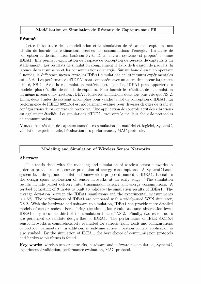
Modelisation et Simulation de Reseaux de Capteurs sans Fil
Resume:
Cette these traite de la modelisation et la simulation de reseaux de capteurs sansfil afin de fournir des estimations precises de consommations d’energie. Un cadre deconception et de simulation base sur SystemC au niveau systeme est propose, nommeIDEA1. Elle permet l’exploration de l’espace de conception de reseaux de capteurs a unstade amont. Les resultats de simulation comprennent le taux de livraison de paquets, lalatence de transmission et les consommations d’energie. Sur un banc d’essai comportant9 nœuds, la difference moyen entre les IDEA1 simulations et les mesures experimentalesest 4.6 %. Les performances d’IDEA1 sont comparees avec un autre simulateur largementutilise, NS-2. Avec la co-simulation materielle et logicielle, IDEA1 peut apporter desmodeles plus detailles de nœuds de capteurs. Pour fournir les resultats de la simulationau meme niveau d’abstraction, IDEA1 realise les simulations deux fois plus vite que NS-2.Enfin, deux etudes de cas sont accomplies pour valider le flot de conception d’IDEA1. Laperformance de l’IEEE 802.15.4 est globalement evaluee pour diverses charges de trafic etconfigurations de parametres de protocole. Une application de controle actif des vibrationsest egalement etudiee. Les simulations d’IDEA1 trouvent le meilleur choix de protocolesde communication.
Mots cles: reseaux de capteurs sans fil, co-simulation de materiel et logiciel, SystemC,validation experimentale, l’evaluation des performances, MAC protocole.
Modeling and Simulation of Wireless Sensor Networks
Abstract:
This thesis deals with the modeling and simulation of wireless sensor networks inorder to provide mote accurate prediction of energy consumptions. A SystemC-basedsystem level design and simulation framework is proposed, named as IDEA1. It enablesthe design space exploration of sensor networks at an early stage. The simulationresults include packet delivery rate, transmission latency and energy consumptions. Atestbed consisting of 9 motes is built to validate the simulation results of IDEA1. Theaverage deviation between the IDEA1 simulations and the experimental measurementsis 4.6%. The performances of IDEA1 are compared with a widely-used WSN simulator,NS-2. With the hardware and software co-simulation, IDEA1 can provide more detailedmodels of sensor nodes. For offering the simulation results at same abstraction level,IDEA1 only uses one third of the simulation time of NS-2. Finally, two case studiesare performed to validate design flow of IDEA1. The performance of IEEE 802.15.4sensor networks is comprehensively evaluated for various traffic loads and configurationsof protocol parameters. In addition, a real-time active vibration control application isalso studied. By the simulation of IDEA1, the best choice of communication protocolsand hardware platforms is found.
Key words: wireless sensor networks, hardware and software co-simulation, SystemC,experimental validation, performance evaluation, MAC protocol.